Accrual duration

Ilia D. Dichev

Emory University

December 15, 2016

Abstract: Accrual duration can be defined as the length of time between an accrual and its associated cash flow. This paper argues that accrual duration is a key factor in understanding the discretion in accruals. The function of accruals is to shift the recognition of associated cash flows across time, usually working in pairs of opening/closing accruals. By design, one side of the accrual pair shifts the recognition of the associated cash flow away from the period in which it occurs by recording an accrual with the same magnitude but the opposite sign in the same period. Thus, such zero-duration accruals are non-discretionary because the timing and magnitude of the associated cash flow pin down the timing and the magnitude of the concurrent accrual. The other side of the accrual pair shifts the recognition of the associated cash flow into some other time period(s), which involves using forward-looking estimates over the duration of the accrual, and therefore some discretion. In addition, accruals that have longer duration are more discretionary because longer horizons of estimation allow more discretion with respect to their timing and magnitude. Summarizing, accrual duration and accrual discretion are inextricably linked by the fundamentals of the accrual process. The study concludes with some thoughts on how to practically use accrual duration as a measure of accrual discretion.

I appreciate helpful comments from Hal White, Valeri Nikolaev, Frank Zhang, Joseph Gerakos, Jim Leisenring, Yin Wang, Xiao Tian, and workshop participants at Rice University, INSEAD, ESSEC (Paris), University of Zurich, Tilburg University, Washington University, University of Miami, Hong Kong Polytechnic University, Chinese University of Hong Kong, UC – Berkeley, University of Tokyo, Kobe University, University of Melbourne, University of New South Wales, and Columbia University.

Contact: Ilia Dichev idichev@emory.edu (404) 727-9353

1

1. Introduction

Recording accruals is at the heart of accounting, and thus there has been much interest in

their function and characteristics. A major theme in this interest is that there is considerable

discretion in recording accruals, and understanding the nature of this discretion is a key to

understanding the utility and cost of using accruals. More specifically, a prominent idea in this

literature is that accruals can be usefully split into discretionary and non-discretionary

components. The motivation is that non-discretionary accruals are driven by fundamentals like

business activity and growth, while discretionary accruals are more subjective, and therefore

more prone to managerial biases and manipulation.1 The volume of the discretionary accrual

literature is substantial. Studies using discretionary accrual ideas or techniques certainly number

in the dozens, and likely in the hundreds (Dechow, Ge, and Schrand 2010 and Francis, Olsson,

Schipper 2008). While this sustained effort has produced a number of insights, the leading

discretionary accrual models have been criticized as inadequate, and even misleading (Dechow,

Sloan and Sweeney 1995, Ball 2013).

Prompted by such criticisms, this study develops a new approach to identifying the

discretion in accruals. The linchpin of this approach is closer attention to how accounting works,

with a special emphasis on the mechanism and manifestations of accrual discretion. The main

idea about the mechanism of accrual discretion is that recording accruals involves using forward-

looking estimates, and it is the quality of these estimates that determines the benefits and the

costs of using accruals. The manifestation of accrual discretion is in shifting the recognition of

cash flows as components of income across time. Note that since income trues up to the

corresponding cash flows, ultimately the only thing that accruals do is re-shuffle the timing of the

recognition of cash flows over time. The implication is that both the benefits and the costs of 1 Many studies also use the term “abnormal accruals,” with a similar meaning.

2

accruals relate to timing, where the benefits of using accruals relate to recognizing cash flows

into the “right” periods, while the costs of using accruals relate to recognizing cash flows into the

“wrong” periods. For example, the benefit of the Accounts Receivable accrual is the more

timely recognition of income (Revenue) at the time of sale as opposed to waiting for cash

collections from customers. The cost of the Accounts Receivable accrual is that income may be

allocated in the “wrong” way, for example the Accounts Receivable may be recorded too early or

it may be overstated at inception which could necessitate restatements or write-downs later on.

As developed in more detail further on, such recording of income into the “wrong” periods

represents timing errors, which introduces noise into the measurement of income.

The difficulty in implementing these ideas is that the main theoretical constructs,

forward-looking estimates and timing errors, are not readily observable. To address this

difficulty, the study looks more closely into the fundamentals of recording accruals. As is well-

known, accruals work in pairs, i.e., the recognition of a cash flow in a period different from when

it occurs is accomplished by recording a combination of an opening and a closing accrual.

Notice that by design one side of this accrual pair coincides in time with the associated cash

flow, while the other side occurs in a different period. The point is that shifting of the

recognition of a cash flow is a two-step process, it is a shifting of a cash flow amount away from

some period and into another period.2

Using the Accounts Receivable example to clarify the difference in the function and

characteristics of these two steps, notice that when cash comes in from customers, the closing

2 For deferrals, the shifting away step comes with the opening accruals (e.g., the capitalization of PPE and Inventory at inception), and the shifting into another period step comes with the closing accruals (recoding the expense of Depreciation and Cost of Goods Sold). For accruals proper, the order of the two steps is reversed – the shifting into another period step comes with the opening accruals (e.g., the recognition of income at the inception of Accounts Receivable and the recognition of expense at the inception of Warranty Payable), and the shifting away step comes with the closing accrual (the extinguishment of Accounts Receivable with cash collections and Warranty Payable with cash payments).

3

accrual of Accounts Receivable is merely a matter of bookkeeping rather than discretion. For

example, if $100 of cash comes in, the Accounts Receivable has to be reduced by $100, there is

no other way to record the collection. In other words, shifting the recognition of a cash flow

away from a period is accomplished by recording an accrual with the same magnitude and the

opposite sign in the same period. Thus, such accruals are non-discretionary because the timing

and the magnitude of the concurrent cash flow pin down the timing and magnitude of the

associated accrual.

In contrast, the opening accrual for Accounts Receivable is discretionary because it can

be recorded sooner or later, and at larger or smaller amounts depending on estimates about

satisfying the revenue recognition criterion and the future cash collections from customers. For

deferrals like PPE and Inventory the sequence is reversed, the opening accrual is non-

discretionary because it is merely the deferral of a known cash flow at a known time, and it is the

allocation of these costs to later periods as depreciation or cost of goods sold where the

discretion resides. The unifying point for deferrals and accruals proper is that recording accruals

away from the periods of their associated cash flows always involves using some kind of

forward-looking estimates (e.g., projected cash flows, useful lives) and therefore it is these

accruals only that embody the notion of discretion in accounting.

This intuition can be formalized and extended by introducing the notion of accrual

duration. Accrual duration can be defined as the length of time between an accrual and its

associated cash flow. The idea is that accrual duration captures the horizon of accrual

estimation, and is therefore closely related to the discretion of accruals. Specifically, accruals

that are concurrent with their associated cash flows have zero duration, and also have zero

discretion because there is no estimation involved – as discussed earlier, the timing and

4

magnitude of the cash flow pin down the timing and magnitude of its associated concurrent

accrual. But recording the other side of the relevant accrual pair involves estimation of future

events, and is thus discretionary in timing and magnitude. Note also that accruals that have

longer duration are more discretionary because estimation is unavoidably less certain over longer

horizons. For example, recording the opening accrual for a 10-month Accounts Receivable is

likely to be more discretionary than that for a one-month receivable. Summarizing, accrual

duration and accrual discretion are inextricably linked by the fundamentals of the accrual

process.

The paper concludes with a discussion of the pros and cons of the accrual duration

approach, and offers some observations on its possible empirical applications. The major

attraction of this approach is that it applies to virtually all possible accruals. The major difficulty

in implementation is the identification of the associated cash flows and accruals because current

financial reporting provides only a patchwork of the necessary data. When the associated

accruals and cash flows are available (e.g., for PPE, revenue accruals), it is possible to derive

estimates of discretionary accruals using exact algebraic derivations, avoiding the vexing

statistical and validity issues that plague existing discretionary accrual models. Absence of clean

data necessitates reverting to statistical estimation, either at the level of individual or aggregate

accruals.

While the accrual duration approach is flexible, and application partly depends on

research goals, it is possible to make some general recommendations. Essentially, the paper

argues for a two-stage approach in the investigation of discretion in accruals. The first stage is

the split of total accruals into discretionary and non-discretionary components along the lines

suggested above. The point is that non-discretionary accruals as defined above have zero ability

5

for discretion, and therefore motivations for discretion are not in play either. Thus, such accruals

are usefully removed from total accruals before pretty much any further investigation of

discretion. The remaining discretionary accruals can be further stratified on relevant dimensions

of firm fundamentals and managerial incentives, consistent with models in existing research (e.g.

Francis, LaFond, Olsson, and Schipper 2005). Accrual duration itself can be used as another

such stratifying variable since accruals with longer duration are more discretionary.

The remainder of the paper is organized as follows. Section 2 offers some observations

on the role of accruals in accounting, and introduces the concept of timing errors in accruals and

income. Section 3 introduces the notion of accrual duration, and outlines its relation to

discretion in accruals. Section 4 discusses the advantages and limitations of the accrual duration

approach. Section 5 suggests some empirical applications. Section 6 concludes.

2. Accrual discretion and errors of timing

2.1 The use of forward-looking estimates in accrual discretion

I start with some observations on the nature of the accrual process, which serve as a

springboard for the main theoretical ideas later. The essence of accrual accounting is the use of

accruals. Accruals can be defined as adjustments to the underlying cash flows, which shift their

recognition as components of income over time. 3 For example, consider a company that makes

$100 of credit sales at time t, and the account is collected at time t+1. The accounting system

records this transaction with the opening and closing of an Accounts Receivable accrual:

Time t Accounts Receivable $100 Sales Revenue $100

3 Notice that this formulation is equivalent to the often-used derivation of accruals as the changes in the assets and liabilities of the firm because of the articulation between the balance sheet and the income statement. The emphasis in this study is on the income view of accruals because leading stakeholders view earnings as the most important number in financial reports, and also because of the desire to link earnings to cash flows.

6

Time t+1 Cash $100 Accounts Receivable $100

Looking more closely at this example reveals that the mechanism of accrual discretion is

through the use of forward-looking estimates. In the Accounts Receivable example, the goal of

the accrual adjustments is to shift the recognition of Sales Revenue (a component of income)

from the time of cash collections at t+1 to the point of sale at time t. The accounting system

accomplishes this goal by recoding at time t a forward-looking estimate of the expected future

cash collections.4

The notion of accrual discretion studied here is broad. Holding other factors constant, it

is defined as the range of possible estimates that can be used in a given transaction. For

example, if an Accounts Receivable with mean expected receipts of $100 can be recorded

anywhere in a range of $98-$102 vs. a range of $95-$105, we can say that there is more

discretion in the latter range. While this definition is quite general and probably non-

controversial, it is clear that operationalizing it is difficult. Especially for outside observers,

measures of the range of possible managerial estimates are unavailable. But as shown later, it is

possible to derive some useful results that capture the spirit of this notion of accrual discretion.

Notice that this notion of accrual discretion is also broad in the sense that it encompasses

everything that may influence the range of possible estimates, including fundamentals like

volatility of operations but also opportunistic managerial motivations like hitting earnings

4 Note that accrual discretion is also governed by factors beyond the use of estimates. For example, standard setting specifies rules that prescribe or restrict the use of discretion in accruals, e.g., U.S. GAAP mandates the capitalization and depreciation of PPE but prohibits the capitalization of most R&D costs even if estimates of future R&D benefits are available. While such other determinants of discretion are important, the emphasis in this study is on the role of forward-looking estimates in accrual discretion. The reason is that the use of estimates is at the heart of accrual discretion, and insights about their role are universal, as seen in more detail further on. In contrast, standard setting is shaped by more idiosyncratic factors including consideration of the relative importance of various firm stakeholders, which triggers the use of compromises and even political meddling.

7

benchmarks and control features like quality of the auditing and corporate governance. For

applications that are interested in more focused notions of discretion, existing research offers

some helpful techniques for splitting broad measures of discretion into more focused

components, e.g., Francis, LaFond, Olsson, and Schipper (2005) split total discretionary accruals

into fundamentals-driven vs. managerial components.

2.2 Errors of timing

Most accrual adjustments work as an associated pair of opening and closing accruals,

where the opening accrual initiates the necessary adjustment, and the closing accrual reverses

and extinguishes the initial adjustment. Thus, by the end of the life of the transaction, the

cumulative net accrual is zero. This property can be stated more formally using the expression:

Earningst = Cash Flowst + Accrualst (1)

Where summing up over the life of any transaction obtains:

∑Earningst = ∑Cash Flowst + ∑Accrualst

And since all accruals reverse over the life of the relevant transaction, the sum of the associated

accruals over time is zero, which yields:

∑Earningst = ∑Cash Flowst (2)

which is true for any transaction, as long as “Earnings” and “Cash Flows” are appropriately

defined.5 Since everything on the income statement and across firm activities is additive, it is

clear that this expression applies to all components of earnings (like specific revenues and

expenses, operating and net income, gains and losses), and for any aggregation at the account,

division, and firm level. It also applies to all kinds of transactions, including those with multiple

5 For example, if “Earnings” is Revenue, “Cash Flows” will be Cash Collections from Customers. Cost of Goods Sold for a merchandising firm will correspond to Cash Paid to Suppliers. Net Income will correspond to Free Cash Flows to Equity Holders.

8

cash flows, and multiple initiating and reversing accruals, e.g., the accounting for Investments

under the equity method.

Of course, expression (2) in itself is nothing new to accounting thought, it is the

expression that underpins well-known intuitions like “accounting is self-correcting” and

“earnings true up to the corresponding cash flows”. But the implications of this expression have

not been fully explored, as reflected in the following observation:

Observation 1: Both the benefits and the costs of recording accruals relate entirely to the

timing of the recognition of the associated cash flows into earnings.

The benefits side is better-understood, and it is clear from expression (2). Since the total

recognized magnitudes are the same across accrual and cash flow accounting, the benefits from

the accrual process have to be in the timing pattern of recognition. Consider, for example, the

following transaction, where the sequence of events and summary implications are organized in

Table 1:

Time t - Company makes a sale for $300, to be collected in three installments of $100 each over

the next three periods (with all discounting effects ignored).

Time t+1 - Customer makes the scheduled $100 payment.

Time t+2 - Customer misses the scheduled $100 payment. The company estimates that the

customer will make the final payment at t+3, and therefore writes down the

receivable to its realizable value of $100 as of the end of t+2.

Time t+3 - Customer makes an actual final payment of $120, and thus the company realizes a

gain of $20.

In this example, total income (revenue) under cash accounting is $220, equal to cash

collected from the customer. Total income (revenue) under accrual accounting is also $220. The

9

only thing that differs across the two systems of accounting is the pattern of recognition over the

four periods, which is 0, 100, 0, 120 for cash accounting, and 300, 0, (100), 20 for accrual

accounting.

Thus, income under accrual accounting is the associated cash flows, sliced and re-

distributed in a different timing pattern. And since the only thing that differs across the two

systems is timing, it follows that the entire benefits of the accruals process have to be somehow

related to timing as well. In this case, the benefit is the more timely recognition of sales revenue

at the time of sale, presumably because that period more accurately represents when the firm

completed its obligations in the sale.6 More generally, the conclusion is that the benefit of using

accruals is in shifting the recognition of the associated cash flows into the “right” periods, where

“right” is prompted by the logic of the business transaction.

The cost side of Observation 1 is less clear, and I believe it is either novel or at least not

widely understood in the accounting literature. On some basic level, since expressions (1) and

(2) show that the only difference between earnings and associated cash flows is the pattern of

recognition over time, it follows that the costs of the accrual process have to be in the pattern of

recognition as well – there is simply nowhere else they can be. But it is less clear what that

means, especially if one wants to operationalize this intuition.

Further reflection on the four-period accounts receivable example above provides some

clues. It is clear that the accruals in this example did not work well because significant

collectability problems came up, and that prompted accrual and income adjustments in the

follow-up periods. The company turned out to be too optimistic in its initial accrual, and was too

pessimistic in the third-period write-down, which necessitated adjustments later on. The main

6 Point is easier to see if there were no collectability problems, with the firm booking $300 at time t, and collecting three installments of $100 thereafter.

10

idea behind booking the effects of the sale into income at the time of sale is that that it represents

a more timely recognition of the accomplishments of the company in this transaction. But note

that the realized pattern in income over the four periods of the transaction was $300, $0, ($100),

$20, which clearly deviates from an ideal pattern of total revenue recognition at the time of sale

of $X, $0, $0, $0.

It is also worth thinking what this amount $X would be under an ideal pattern of revenue

recognition at the time of sale. Ideally, the company would have liked to recognize all relevant

revenue at the time of sale, which is equal to the total realized cash collection of $220. In other

words, if the company had perfect foresight in this transaction, it should have booked $220 as

revenue and opening receivable at the time of sale, and then the cash collections would have

amortized the receivable, with no effect in income, with a resulting pattern of income recognition

of $220, $0, $0, $0. Compared to that, the actual pattern of recorded income of $300, $0, ($100),

$20 implies that the company booked $80 of income too much in the first period, and then that

was corrected by a loss of $100 in the third period, and finally zeroed out with a gain of $20 in

the fourth period. In other words, the costs of using accruals in this example is that pieces of

income end up booked in the “wrong” periods. One can think of income ending up in the wrong

periods as “timing errors”, as errors in the timing of recognition of income.

Summarizing, the benefits of the accrual process are in shifting the recognition of cash

flows into the “right” periods, where “right” is determined by the business substance of the

transaction. The costs of the accrual process are in shifting the recognition of cash flows into the

“wrong” periods, where “wrong” is again determined by the business substance of the

transaction.

11

The difficulty in using these conclusions is that typically it is not clear what “right” and

“wrong” periods really means, especially for an outside observer that does not have access to the

transactional records of the company. Notice also that even with great records, the income

effects of transactions are only clear ex post, while evaluation of accrual and earnings quality is

needed on an evolving and ex ante basis. In the accounts receivable example above it is clear ex

post that the time-of-sale recognition of income was compromised by unforeseen collectability

problems. But it is not clear whether something meaningful can be said about these collectability

problems before they manifest. As an illustration of these problems, notice that the initial

accrual of $300 at time t turns out ex post to be a jumble of a “right” accrual of $220 and

“wrong” over-accrual of $80. The question again is whether some meaningful differentiation

can be made on an ex ante basis, and for an outside observer.

It turns out that although this problem is vexing, some progress can be made by looking

more closely into the mechanism of accrual discretion discussed earlier. The main insight is that

since accrual accounting moves the recognition of income across time using forward-looking

estimates, it is the use of these estimates as opposed to actual realizations which creates “timing

errors”, i.e., the problem of income ending up in the wrong periods. The example above is a

good illustration of this insight. Booking revenue at the time of sale seems warranted because it

more accurately reflects the fact that the benefits of the sale transaction are mostly secured at the

time of sale rather than waiting for the cash collections to roll in as in cash accounting. But this

benefit comes at the cost of booking revenue as a forward-looking estimate of cash collections,

and the resulting difference between estimate and realizations necessitates recording corrections

in income in later periods. These corrections are essentially errors in the timing of the

12

recognition of income, and constitute the cost or recording the revenue accrual at the time of

sale.7

A closer look into the example also offers a way to conceptualize this intuition. The idea

is that if one could construct a theoretical benchmark of recoding accruals which avoids the

problem of using estimates and therefore avoids timing errors, one would be left with only the

benefits of accruals, providing a clean split of accruals and income into their “right” and “wrong”

components. In this case, there is a natural solution. Since the problem is that forward-looking

estimates differ from their realizations, the solution is the use of “perfect foresight” estimates. In

the accounts receivable example above, the “perfect foresight” estimate is recording $220 at the

time of sale because that amount is a perfect foresight of the expected cash collections. As

discussed above, the “perfect foresight” estimate of the accounts receivable accrual of $220 at

time t also produces the “perfect foresight” pattern of revenue recognition of $220, $0, $0, $0.

The perfect foresight accrual of $220 at time t also produces a quantifiable measure of the

“timing errors” in this example, i.e., income ending up in the “wrong” periods. Since Actual

Income = Perfect Foresight Income + Timing Errors for any given period, it follows that:

Timing Errors = Actual Income – Perfect Foresight Income (3)

Using this expression, and recalling that the pattern of actual income is $300, $0, ($100), $20 and

that for perfect foresight income is $220, $0, $0, $0, yields a sequence of timing errors of $80,

$0, ($100), $20, also see a summary of income and timing error effects in Table 1. This

sequence of timing errors correctly reflects the intuition that the company overestimated the

initial receivable by $80 at time t, corrected the initial mistake at time t+2 by recording a $100

write-down (so, ended up overshooting the right correction by $20), and finally the series of

7 By “cost of using accruals” what is meant here is the cost of using income as a performance metric. Otherwise, there are clearly other costs of using accruals like procedural costs of running the accrual accounting system, auditing, etc.

13

errors and corrections was settled with a positive adjustment of $20 at time t+3. Note that the

sequence of timing errors sums up to zero, consistent with the intuition that accrual accounting is

self-correcting.

Summarizing, the derived sequence of timing errors is a measure of the cost of using

accruals. The cost of using accruals arises from the necessity of using forward-looking

estimates, and since the estimates differ from realizations, the result is that recorded income

includes temporary and reversible errors of timing.

Introducing the concept of timing errors as the key cost of using accruals offers two

decisive advantages over existing notions of accrual discretion and accrual quality. First, it is

rooted into the fundamentals of the accrual process, which is preferable to ad hoc models like

Jones (1990) and its extensions. Second, the notion of timing errors applies to virtually all

accruals, which is preferable to other models, which typically capture only one type of accruals

and/or one type of discretion. For example, the Dechow and Dichev (2002) model captures the

discretion of only short-term accruals, where the opening accrual precedes the associated cash

flow (i.e., accruals proper, for example one-period Accounts Receivable and Warranty Payable).

In contrast, the notion of timing errors also applies to deferrals, for example Inventory and PPE.

And the notion of timing errors accommodates both short-term and long-term accruals, and

readily applies to all kinds of operating, investing, and financing accruals.

A brief example using the long-term PPE/depreciation deferral illustrates the universal

applicability of the timing error approach. Assume that a company buys PPE for $100 at the end

of year t, expected to be depreciated straight-line over the next four years, with no salvage value.

Accordingly, depreciation for year t+1 is $25. In year t+2, however, the company determines

that the PPE is obsolete, and so records a total depreciation/write-off of $75 to reduce its value to

14

zero. The benefit from using accruals in this example is that the cost of PPE is not immediately

expensed at inception but is rather spread out over the useful life of equipment, which makes

sense given the economics of PPE investment. The discretion and cost from using forward-

looking estimates here comes from the forward-looking estimate of depreciable life. The

recorded pattern of depreciation expense (broadly defined to include write-offs) is $25, $75 over

the two-year realized life of the equipment. The “perfect foresight” estimate of depreciable life

would be two years, and correspondingly the “perfect foresight” pattern of straight-line

depreciation expense is $50, $50. The resulting pattern of timing errors in accruals and income

is ($25), $25, which correctly reflects the intuition that the company recorded too little

depreciation in year t+1, and too much in year t+2. Note again how the cost of using forward-

looking estimates in accruals manifests as temporary and reversible timing errors in income.

From this example, it is also clear how the timing error approach can be extended to other

deferrals, e.g., Inventory, Prepaid Expenses, Deferred Revenue, etc.

To further understand the timing error approach, a comparison with the Dechow/Dichev

(DD) model is instructive. Essentially, these two approaches share the same underlying logic but

the timing error approach can be considered a more general version of the DD model. The

reason is that the DD model is also a “perfect foresight” approach, where the key intuition is that

the quality of accruals is determined by the extent to which accruals map into their future cash

flow realizations. In other words, the DD approach uses perfect foresight with respect to the

magnitude of the associated future cash flows as the benchmark for “right” accruals. And since

the quality of accruals in DD is determined by the deviations of accruals from the perfect

foresight forecast of the associated future cash flows, the takeaway is that DD estimations errors

are one manifestation of the broader concept of timing errors.

15

In comparison, the timing approach is a more general version of the DD approach

because it uses perfect foresight with respect to everything as a benchmark for “right” accruals.

For example, perfect foresight could mean correct estimation of not only the magnitude of future

cash flows but also of depreciable lives and salvage values for PPE, of future construction costs

for revenue recognition under the percentage-of-completion method, of estimates of future

profitability in accruing incentive compensation expense, of the timing, magnitude, and discount

rates for anticipated cash flow related to contingent liabilities and legal settlements, and so on.

For the interested reader, Appendix A provides additional information and examples on the

comparison between the DD model and the timing error approach.

Summarizing this section, the benefit of using accruals is the more timely recognition of

income, which makes it a better measure of firm performance. The cost of using accruals arises

from the need to make forward-looking estimates, which introduces timing error noise in the

recognition of income. These main ideas are reflected graphically in Figure 1. Figure 1

compares the anchor case of cash flow accounting to the benchmark case of accrual accounting

under perfect foresight, and the actual accrual accounting using forward-looking estimates. The

difference between cash flow accounting and perfect foresight accounting establishes the

benchmark maximum possible benefit from using accrual accounting. The difference between

perfect foresight accounting and actual accrual accounting is errors of timing, which are the cost

of using estimates in accruals. The difference between cash flow accounting and actual accrual

accounting establishes the net benefit from using accrual accounting.

3. Accrual duration

16

While the notion of timing errors has intuitive appeal, operationalizing it is non-trivial.

In some cases, it may be possible to measure timing errors directly. For example, actuarial gains

and losses in pension accounting are clearly timing errors, and they can be identified from

footnote disclosure. Income effects from changes in depreciable lives also represent timing

errors, and they are disclosed in the footnotes as well. Most timing errors, however, are difficult

to identify because they result from all kinds of realizations differing from estimates, and most

such data are not available to outside users.

As a solution, this paper proposes a further development and reformulation of the

estimates and timing error approach, which relies on closer attention to how the accrual process

works. As is well-known, accruals generally work in pairs, where the combination of an opening

and a closing accrual shifts the recognition of a cash flow into income to a period different from

when the cash flow occurs. For an example for deferrals, consider a firm that buys $100 of

merchandise inventory for cash. The corresponding accrual pair will be reflected in the

following two journal entries, which occur at two different points in time:

Inventory $100 Cash $100 Cost of Goods Sold $100 Inventory $100

The opening accrual for Inventory defers the recognition of the cash outflow away from

the period in which the purchase occurs, and the closing accrual shifts the recognition of that

cash outflow in the form of Cost of Goods Sold into the period in which the Inventory is sold.

Similar patterns are observed for other deferrals like PPE, Prepaid Rent, and Deferred Revenue.

17

For accruals proper, the opening accrual occurs before the associated cash flow, and it is

the closing accrual that coincides with that cash flow. For example, for $50 of Accounts

Receivable (and assuming no collectability problems for now), the journal entries are:

Accounts Receivable $50 Sales $50

Cash $50

Accounts Receivable $50

Similar patterns are observed for other accruals proper, including all kinds of receivables

and payables like Interest Receivable, Accounts Payable, and Warranty Payable.

The unifying message across these two examples is that no matter whether we are dealing

with deferrals or accruals proper, by design one side of the accrual pair coincides with the

associated cash flow, and the other side occurs in some other period. This is, of course, not

accidental because moving the recognition of a cash flow into income across periods involves

two steps, one is moving the recognition of the cash flow away from a period, and the other one

is moving the recognition of the cash flow into another period. As the two examples above

illustrate, the accrual that coincides with the associated cash flow is the device that moves the

recognition of a cash flow away from that period, and the associated accrual that occurs in some

other period is the device that moves the recognition of the cash flow into this other period.

One key implication is that the timing and magnitude of the underlying cash flow pin

down the timing and the magnitude of its associated concurrent accrual. This exact

correspondence obtains by construction - if the recognition of a cash flow of a certain magnitude

is to be moved away from a certain period, the only way to do that is by recording an accrual

with the same magnitude and the opposite sign in that same period, so that the net effect on

income is zero. Thus, such accruals are non-discretionary. In the Inventory example above, the

18

opening accrual is non-discretionary because if a firm pays $100 for Inventory (negative cash

flow), it has to put this Inventory on the books for $100 (positive accrual of $100); thus,

recording this accrual is simply a matter of bookkeeping, and not really of a matter of estimation

or discretion. This point is easy to see using the representation Earnings = Cash Flows +

Accruals, which for the opening accrual of Inventory is:

Cost of Goods Sold = Cash Spent on Inventory + Inventory

0 = -$100 + $100

In other words, since accrual accounting suggests that the cost of Inventory should be deferred

until sold rather than immediately expensed at purchase, the only way to defer the cost of

purchase until some future period is to record an Inventory accrual with the same magnitude but

the opposite sign in the period of the associated cash flow. This is a bookkeeping identity rather

than a matter of discretion.

Using the terminology of this paper, it is also easy to see that accruals that coincide with

their associated cash flows have no discretion. The reason is that the cash flow and the

associated concurrent accrual coincide in time, and so the time horizon of estimation for that

accrual is zero. The implication is that the actual recorded accrual and the “perfect foresight”

accrual are the same, and so there is no estimation or discretion or timing errors for such

accruals.

The other side of the Inventory accrual, however, is where the estimation and the

discretion is. Depending on whether the firm is using FIFO or LIFO, periodic or perpetual

inventory system, and whether there are inventory write-downs, the realization of the Inventory

cost into income could take a number of different trajectories, and there is real managerial

discretion in charting these trajectories. In other words, there is a time horizon of estimation, and

19

so there is a difference between recorded and perfect foresight accruals, and so there is both

discretion and possible timing errors in accruals. Summarizing, accruals that are concurrent with

their associated cash flows are non-discretionary, while accruals that occur in a period away

from their associated cash flows are discretionary.

Note that this intuition applies to virtually all accruals. With Accounts Receivable, the

opening accrual is the discretionary one because management has discretion with respect to both

its timing and magnitude, while the receipt from customer automatically triggers both the timing

and the magnitude of the closing accrual. Warranty Payable is an accrual proper, and indeed the

recording of warranty expense, which is the opening accrual for Warranty Payable is where the

discretion is, while the payment of warranty claims pins down the timing and the magnitude of

the closing accrual; similar reasoning applies for all kinds of reserve accounts like provisions for

environmental remediation, provisions for workforce reductions, provisions for taxes, provisions

for integration of acquired businesses, and so on. PPE is a deferral, which implies that the

opening accrual should be non-discretionary, while the closing one is discretionary. Indeed, the

timing and the magnitude of cash spent for PPE pin down the opening PPE accrual, while

management has considerable latitude with respect to the timing and magnitude of the (series of)

closing PPE accruals of Depreciation Expense, and possibly PPE write-downs.

A way to formalize and extend this intuition is to introduce the notion of accrual

duration. Accrual duration can be defined as the length of time between an accrual and its

associated cash flow. For example, for a $1,000 accounts receivable that is opened on March 1,

and is closed at the receipt of customer collections on June 1, the accrual duration for the

opening accrual is three months, and for the closing accrual it is zero. It is immediate that

accruals that are concurrent with their associated cash flows have zero duration. And since such

20

accruals have zero estimation and discretion, there is a tight link between accrual duration and

accrual discretion at the focal and common point of zero duration.

Further consideration reveals that the relation between accrual duration and accrual

discretion extends to the full range of accrual duration, where the discretion in accruals increases

in accrual duration. Everything else equal, recording warranty expense on three-year contracts is

likely to produce more discretionary accruals than those for one-year contracts. Depreciation

expense on PPE with projected life of 20-30 years is likely to be more discretionary than that for

PPE with a one-year life. The reason is straightforward, longer duration implies longer horizon

of estimation, and longer horizons unavoidably bring more uncertainty and discretion for the

resulting estimates.8 We also have some evidence that forecasting horizon is rather strongly

related to uncertainty in business, e.g., the predictability of earnings and growth deteriorates fast

with forecast horizon (Chan, Karsecki, and Lakonishok 2003). Thus, there are reasons to believe

that accrual duration is a powerful determinant of discretion in accruals.

4. Discussion

This section provides a discussion, and some extensions and clarifications of the theory in

the paper. A broad advantage of the accrual duration approach is simply a better understanding

of the nature and function of accruals, which allows new conceptual clarity into some long-

standing issues. As an illustration of this advantage, consider the example of a steady-state

company with no changes in assets and liabilities. Can such a company have a change in its

accrual quality over a given period? Intuitively, the answer must be “yes.” But the traditional

8 For Accounts Receivable, the estimate is how much cash will be collected, for Warranty Payable the estimate is how much cash will be paid out in claims, for Depreciation the estimate is about the length of useful life, for Revenue under the percentage-of-completion method the estimate is about the remaining costs to complete the project, and so on.

21

understanding of accruals as changes in assets and liabilities will be flummoxed by this question,

because a steady-state company has no change in net assets, and so it does not have accruals, and

therefore cannot have a change in accrual quality.

In contrast, the approach advocated here handles such a question with ease. Take

Accounts Receivable, for example, that has no change over a given period. The accrual duration

approach will point out that although the net change in Accounts Receivable is zero, there are

new gross accruals recorded during the period, specifically the old Accounts Receivable have

been collected, and there have been an equal amount of new Accounts Receivable created by the

new credit Sales (see also White 2012 on this point). And since the new Accounts Receivable

can be of lower quality than the old Accounts Receivable, it is clear that accrual quality can

change for steady-state firms. The key point is that the accrual duration approach makes a sharp

distinction between the reduction of receivables due to the collection of cash (a non-discretionary

accrual) and the origination of new receivables (a discretionary accrual), while the traditional

approach essentially treats them as the same accrual but with opposite signs. This is a

consequential distinction.

Another example of enhanced conceptual clarity is the question of the contemporaneous

correlation between accruals and cash flows. Many studies have explored this question,

generally finding a negative correlation (Dechow 1994), which has been decreasing over time

(Bushman, Lerman, and Zhang 2016), while some studies have pointed out that this correlation

can be positive in certain environments (e.g., recessions trigger poor cash flow from operations

coupled with write-offs of assets as in Ball and Shivakumar 2006). There has also been much

debate about the magnitude and interpretation of the negative correlation between cash flows and

accruals, with some authors interpreting it as a beneficial sign of resolving timing and

22

mismatching problems in the cash flows (Dechow 1994), and others interpreting it as evidence of

opportunistic managerial smoothing of income (Leuz, Nanda and Wysocki 2003).

While a full reconciliation of extant evidence and views is beyond the scope of this study,

the accrual duration framework yields some key observations that can be helpful in

understanding the theoretical and empirical correlations between cash flows and accruals. Most

importantly, it is clear that the correlation for associated contemporaneous cash flows and

accruals is negative, and in fact it is -1 if both variables are appropriately defined. Note also that

this negative correlation obtains before any value-laden functions of accruals are posited, it is

simply the unavoidable outcome for any accrual system that moves the recognition of cash flows

across periods because that requires recording contemporaneous accruals with the same

magnitude and the opposite sign of the associated cash flow. If one is going to capitalize the

cash cost of PPE of $100, there is no other way to do that than by debiting an asset, a positive

accrual, which will be perfectly negatively correlated with the corresponding contemporaneous

cash outflow of $100.

Thus, one conclusion from these considerations is that the negative correlation between

cash flows and contemporaneous accruals is an unavoidable and necessary property of accruals.

This impression is further strengthened by the point that such accruals are non-discretionary, as

one can recall from the analysis presented earlier in the paper. Of course, things become more

complicated when one is using non-associated cash flows and accruals. But that is precisely the

point – a major takeaway from this study is that there has to be better care in the definition of

cash flows and accruals used in a given specification. Many examples are possible here, e.g.,

Cash Flow from Operations from the Statement of Cash Flows is not really “cash flow from

23

operations” because it includes many non-operating items, and this contamination has likely

become worse over time because of the proliferation of non-operating items.9

It is also useful to point out that while the preceding theoretical framework uses the

simplifying notion of “accrual pairs,” the main ideas of the study generalize to more complicated

accrual situations. For example, consider the accounting for equity investments, which for

similar securities could be under the cost or the equity or one of the fair value methods. For all

these methods, the initial accrual for the purchase of the investment and the final accrual for the

sale of the investment are non-discretionary because they are pinned down by the concurrent

cash flows. But accounting for the intervening years can take very different trajectories, with no

entries (except for dividends) under the cost method, following book profitability under the

equity method, and following market values under the fair value methods. And that is precisely

the point, all of these intervening entries are discretionary because there are no associated

concurrent cash flows. Similar considerations apply for other more involved accrual situations,

for example, booking accounts receivable with a bad debt expense provision, and the subsequent

collection and write-offs of receivables. Appendix B provides examples of some common

accounting situations, and how the accrual duration approach applies to them.

The notion of accrual duration is also appealing because it provides a conceptual

generalization for some existing techniques and measures in accounting. For example,

accounting texts point out that high value of Days Receivables Outstanding is a sign of low-

quality Accounts Receivable. As is probably clear, Days Receivables Outstanding, defined as

9 The accrual duration approach also offers insights about the correlation between non-contemporaneous cash flows and accruals. For associated cash flows and accruals, most non-contemporaneous correlations will be positive because the non-contemporaneous accruals are essentially accruing the effect of the associated cash flow into income in another period, and so they have to be of the same sign. In fact, if there is only one non-contemporaneous accrual, and there are no timing errors, the correlation will be 1. But the correlation will be lower, and possibly much lower, if the non-contemporaneous accrual is split into several periods (like in depreciation) and there is timing error noise.

24

Average Accounts Receivable/(Annual Sales/365), is a close kin of accrual duration of the

Accounts Receivable accrual at the account-year level. In fact, the only difference is that Days

Receivables Outstanding measures the number of days it will get all outstanding Receivables to

get collected, while accrual duration for the average Receivable will be half that. Similar

considerations apply for Days Inventory Outstanding, Days Payables Outstanding, and

Depreciable Life. While such measures are widely used, to my knowledge there has been little

attempt to conceptualize and generalize them in a meaningful way.

Finally, it is also helpful to be clear about the boundaries of the accrual duration

approach. The main point here is that this approach takes the accruals as given, i.e., as

mentioned earlier, this approach does not address questions like whether the accruals should

have been recorded in the first place, e.g., in capitalization vs. expensing decisions for R&D, or

standard-setter questions like whether GAAP should capitalize all leases. Further reflection

suggests that this limitation is mild. For one thing, the very same caveat applies to all existing

accrual models, including Jones (1991) and Dechow and Dichev (2002), and their variations and

extensions. The other consideration has to do with utility. On some level, all accruals are

“discretionary” because firms can in theory use cash flow accounting, and eliminate all accruals.

But such an extreme perspective is not helpful. The point is that GAAP already mandates

accruals, and thus in practice there is no way for firms to avoid recording them. Therefore, the

emphasis in this paper is on the pragmatic - since accruals are already being recorded, the

pragmatic question is whether one can perform a meaningful split of total recorded accruals into

more or less discretionary components. And that is the question that this paper answers.

It is also worth considering that standard setting-type issues are notoriously tricky

because they reflect things like balancing the needs and preferences of different societal groups

25

(e.g., equity vs. debt investors vs. government authorities vs. general public), and thus they

inevitably tend to lean to the compromise and to the political. In contrast, the main features of

the approach advocated here apply regardless of what the present GAAP rules may be, and how

they may change in the future. The reason is that accrual duration approach focuses on the

mechanism and consequences of making forward-looking estimates, which applies to any

plausible accrual system.10

5. Possible empirical applications

The accrual duration approach has wide reach, and so specific empirical implementations

depend on the goals of different investigations. Nevertheless, it is useful to offer some broad

observations on possible empirical applications.

As an immediate suggestion, this paper advocates a two-stage approach to investigating

the discretion in accruals. The first stage splits accruals into discretionary and non-discretionary

along the lines discussed above. The non-discretionary accruals are the no-estimation, zero-

duration accruals, whose timing and magnitude are pinned down by the timing and magnitude of

their concurrent associated cash flows. Such accruals are really bookkeeping placeholders,

shifting the recognition of cash flows away from the period in which they occur, and setting the

stage for the other side of the accrual entry where the real discretion in accruals is exercised.

The point is that such accruals are usefully expunged as a first screen no matter what the specific

10 Another caveat about the approach of this paper is that it does not reflect discretion with respect to the management of real activities and cash flows. Partly, this is simply beyond the scope of the study; and this caveat applies to all other accrual models. But in terms of practical import, it is helpful to point out that the conclusions of the study apply regardless of whether there is real earning management. This point is clear for management of cash flows that enter income directly, e.g., cutting R&D to boost income, because there is no interaction with accruals. And it also applies for management of real activities with interaction with accruals, e.g., using an end-of-period sales incentive to boost credit Sales. Notice that whether the sales boost is artificial or not, the same conclusions apply for the accruals produced (Accounts Receivable or Deferred Revenue) – one side of these accrual pairs is tightly determined with respect to timing and magnitude while the other one is not, and the discretion increases in the horizon of the accruals.

26

further investigation is about because if the ability for accrual discretion is not there, specific

motivations like hitting earnings benchmark cannot be in play either. Given that this first stage

would potentially remove up to 50% of accrual variation (roughly, as removing the variation

from one side of accrual pairs), it is easy to see how this first stage would make a difference.

If the relevant cash flow and accrual data are available, the application of the first stage is

exact, avoiding the need for problematic statistical estimations. Using the expression:

Discretionary Accruals = Total Accruals - Non-discretionary Accruals

and having in mind that:

Non-discretionary Accruals = - Concurrent Associated Cash Flow

because non-discretionary accruals shift the recognition of concurrent associated cash flows by

recording the same amount with an opposite sign yields:

Discretionary Accruals = Total Accruals + Concurrent Associated Cash Flows (4)

In expression (4), accounts appear with their algebraic sign given by the way they affect

income. Specifically, cash inflows appear as positive and cash outflows appear as negative, and

increases in assets appear as positive accruals, while increases in liabilities appear as negative

accruals, with the converse for decreases in assets and liabilities.

While this decomposition is simple, there has to be some care in its application. The

difficulty is that while the effects analyzed above are clear at the level of the individual

transaction, such granular data are not available to outsiders. Broadly speaking, the least

aggregated data available to outsiders is at the account-period level. The challenge in using such

aggregated data is in constructing the right “associated” accrual and cash flow variables.

27

For some situations, the application is straightforward. For example, assume that Net

PPE goes up by $10 for period t, and purchases of PPE are $100 during period t with no sales of

PPE. These data yield:

Total PPE accrual = ΔPPE = $10

Associated Cash Flow = Purchases of PPE = - $100

Discretionary PPE accrual = Total PPE accrual + Purchases of PPE = - $90

The -$90 answer represents Depreciation Expense for the period, which makes sense

because Depreciation is where the discretion resides in the PPE accruals; the sign is negative

because Depreciation Expense reduces income. To recap, note that by the end of this example,

the PPE accrual has been cleanly split into a discretionary and non-discretionary component,

with no need for any statistical estimation. This is a powerful advantage considering that

existing discretionary accrual models suffer from major estimation and statistical noise problems,

e.g., the Jones model and its variations, see Dechow, Sloan and Sweeney (1995), Dechow, Ge,

and Schrand (2010) and Ball (2013).

For other situations, it is trickier to figure out what “associated” cash flows and accruals

implies – but as long as the right data are available, exact answers still obtain. The following

example for Accounts Receivable illustrates this point. Suppose that beginning Accounts

Receivable is $30, ending Accounts Receivable is $50, and Sales are $300 during that period

(assume all on credit). What is the Discretionary Accrual for this period? Note that there are no

cash flows associated with the ending balance of Accounts Receivable, and the cash flows

associated with the beginning Accounts Receivable are $30, which represents the collection of

the receivables outstanding at the beginning of the period, also corresponding to the closing non-

discretionary accrual of these receivables. Using this argument and expression (1), the estimate

28

is Discretionary Accruals = $20 + $30 = $50, which is also the ending balance of Accounts

Receivable. This answer makes sense because it indeed captures the discretion in newly-

originated Accounts Receivable during a period, which are not resolved by cash collections by

the end of that period. Using similar logic, this same answer is also suggested in White (2012),

linking the discretion in working capital accruals to their ending balances rather than to their

changes.

In many cases, however, there will be no clear identification of the associated cash flows

and accruals, e.g., for various aggregate specifications like working capital or total accruals. In

such cases, the solution is to revert to some kind of statistical estimation. Specifically, using the

main theoretical conclusion that discretionary accruals are those that are not associated with

concurrent cash flows, the exact theoretical expression (4) is then proxied by the following

regression specification:

Accrualst = b0 + b1*Associated Cash Flowst + εt (5)

where the key to successful identification is to define accruals and cash flows as closely as

possible to their theoretical counterparts in expression (4). Discretionary accruals for time t are

given by the residual term εt, and non-discretionary accruals for time t are calculated as Accrualst

– εt. For example, for the most popular working capital accrual specification, Accruals can be

defined as change in non-cash working capital (ΔWC), and the closest correspondence to

Associated Cash Flows is Cash Flow from Operations (CFO) or some modification which purges

it from non-operating items. It is possible that the accrual duration approach can be adapted to

other aggregate specifications, including those for all accruals of the whole firm or even at the

level of the industry or the entire economy. Note that the change in working capital version of

expression (5) has already been used in existing research, variations of it have appeared for

29

example in Ball and Shivakumar (2006) and Bushman, Lerman, and Zhang (2016), usually

motivated by the noise reduction role in accruals suggested by Dechow (1994) and Dechow,

Kothari, and Watts (1998). In that sense, the specification in expression (5) is an affirmation of

existing practices in accruals research - but is also a call for careful specification of the

associated variables.

Whether the derivation is exact or statistical, the end result of the first stage is a split of

total accruals into discretionary and non-discretionary components. Note that the discretionary

accruals are derived entirely at the level of the firm/account and the period, avoiding the need for

multiple periods and forward-looking information like in Dechow/Dichev applications. Finally,

the discretionary accrual is signed, which is superior to unsigned approaches.

The second stage depends on the goals of the investigation. One way to describe the

broad intuition here is that nearly all existing studies of accrual discretion and accrual quality can

be run as a second stage on the discretionary accruals derived after the first stage above. For

example, one can use proxies for firm fundamentals like size, incidence of losses, and CFO and

sales variability as in Francis, LaFond, Olsson, and Schipper (2005) to split the discretionary

accruals derived in the first stage into fundamentals-driven vs. manager-driven components.

Further, the manager-driven components can be used to test theories of earnings management to

beat benchmarks, and influence capital market and contractual outcomes.

The second stage can also benefit from further stratification on accrual duration because

longer accrual duration unavoidably implies more accrual discretion. Note that the accrual

duration approach centers on the ability for accrual discretion, so it is perhaps a natural

complement to most existing research, which emphasizes the motivation for accrual and earnings

malfeasance. In some cases, the calculation of accrual duration presents no problems. Using

30

well-known techniques from financial statement analysis, it is easy to compute accrual duration

for the discretionary accruals of Depreciation and Accounts Receivable, for example. Assuming

straight-line depreciation and negligible residual values:

Accrual duration for Depreciation = Depreciable life of PPE/2

Where Depreciable life of PPE estimated as Gross PPE/Depreciation Expense, and depreciable

life is scaled by 2 since depreciation is an annuity rather than a single closing accrual. As

mentioned earlier, for Accounts Receivable accrual duration at the account/year level is given by

the Days Receivables Outstanding/2.11

An advantage of the accrual duration approach is that it allows more focused

investigations of accruals, which can potentially improve research design. For example, we

know that revenue recognition problems are the most prominent form of earnings malfeasance,

present in about half of firms with AAERs (Dechow, Ge, Larson, and Sloan 2011), and so some

studies focus on this particular area of accounting discretion (Peterson 2011, Altamuro, Beatty,

and Weber 2005). Existing financial data allows using the accrual duration approach to build

empirical measures at the level of the Revenue account, and its most closely associated accruals,

Accounts Receivable and Deferred Revenue. One can use such information to derive Cash

Collections from Customers, and thus one would have both the relevant cash flow and its

associated accruals, which allows splitting the revenue accruals into discretionary and non-

discretionary components, and deriving measures of accrual duration.

In other cases, there may be a natural focus on specific accruals, especially if the requisite

data are available. For example, required disclosure in the property-casualty insurance industry

provides information about the provision for claims, balances of unpaid claims, and cash paid for

11 This formulation assumes that all Sales are credit sales. If that is not the case, one should instead use credit sales only, if that information is available.

31

claims (Petroni 1992, Beaver and McNichols 1998), which allows constructing measures of

discretionary accruals and accrual duration for the most important accrual for such firms.

Pension and OPEB disclosure about the associated cash flows and accruals can be used to derive

measures of Pension and OPEB discretionary accruals.

6. Conclusion

This paper argues that making estimates is at the heart of using accruals, and that the

quality of these estimates unavoidably depends on the horizon of estimation. This idea is

embodied by the concept of accrual duration, defined as the length of time between an accrual

and its associated cash flow. There are two main results from the analysis of accrual duration.

First, accruals act in pairs, using an opening and a closing accrual to shift the recognition of cash

flows across time. The point is that to shift the recognition of a cash flow away from a period,

by construction one side of the accrual pair has to occur in the same period with the associated

cash flow, and have the same magnitude and the opposite sign. Thus, such zero-duration and

zero-estimation accruals are non-discretionary; essentially, they are bookkeeping placeholders in

the accrual process, setting up the stage for the real discretion in accruals, which is contained in

the other side of the accrual pair. Second, for accruals that shift the recognition of cash flows

into another period, longer duration implies longer horizons of estimation, and therefore more

discretion in the timing and magnitude of recorded accruals. These two results can be used to

derive empirical measures of discretion in accruals. The principal advantage of this approach is

that it applies to pretty much all accruals.

32

Appendix A: Further comparison of the Dechow/Dichev and the timing error approach

The main advantage of the Dechow/Dichev (DD) approach is that future cash flow realizations provide a crisp benchmark for whether accounting records the “right” accruals. The disadvantage is that the DD approach only reflects the discretion in accruals where the opening accrual precedes cash flow realization, e.g., accruals proper like Accounts Receivable and Accounts Payable, and does not capture the discretion in accruals where the cash flow realization coincides with the opening accrual, e.g., deferrals like PPE and Inventory. In addition, the DD approach is designed for working capital accruals, while it is clear that there is much discretion in longer-term accruals. Finally, even in accruals proper there is a timing discretion that is not reflected in the DD approach. For example, premature revenue recognition is not detected by the DD approach as long as the recorded Accounts Receivable is an accurate predictor of cash collections.

The main advantage of the timing error approach is that it applies to all accruals and captures all discretion related to using estimates. The disadvantage is that the timing error approach lacks a natural crisp benchmark for the “right” accruals. Otherwise, the DD and the timing error approach have a common logic because both are “perfect foresight” approaches. In DD, perfect foresight is with respect to the future cash flow realizations. In the timing error approach, perfect foresight is with respect to everything (future cash flow realization, future costs for the percentage-of-completion revenue recognition method, future income in recoding incentive compensation accruals today, depreciable lives, residual lease values, interest rates, etc.), which is of course more general – but harder to operationalize.

A brief example helps in comparing and contrasting these two approaches. Assume that a firm books $100 in Accounts Receivable at time t but only collects $80 in t+1, which triggers a write-off of $20 in t+1. This is a classic DD situation dealing with the discretion for accruals where the opening accrual precedes the cash flow realization. The DD model interpretation of this situation is that the opening Accounts Receivable accrual had an estimation error of $20 ($100 receivable - $80 cash flow realization), which implies a fairly low quality of the Accounts Receivable accrual at time t. The timing error approach reaches a similar conclusion but couches it in different terms. First, the timing error approach points out that total cash flow income over the two periods is $80, and total accrual income is $80 as well ($100 credit revenue at time t - $20 write-off at time t+1). In other words, while there is a mismatch between the opening accrual at time t and cash flow realization at time t+1, there is no mismatch between the total magnitude of accrual and cash flow income over the life of the transaction. The only difference between accrual and cash flow income is the timing pattern of realization. Since the example is simple, it is also intuitively clear what the problem is: essentially, the firm booked $20 of income “too much” at time t but will also have $20 of income “too little” at t+1, when the inflated receivable is written off as a loss. In other words, the mis-estimation of the opening receivable is just a timing error of $20 of income appearing at time t rather than at time t+1. Or in the language of this paper, the actual pattern of accrual income was $100, ($20) over the two periods. The pattern of “perfect foresight” accrual income is $80, 0, which implies a pattern of reversible timing errors of $20, ($20). Thus, DD estimation errors represent a type of timing error – which is not surprising because perfect foresight with respect to cash flow realizations represents one type of perfect foresight.

Note that the more general timing error approach captures additional aspects of discretion and accrual quality even for accruals proper, which are the natural forte for the DD model. For example, consider premature recognition of revenue. Booking $100 of revenue prematurely in period t vs. t+1 is not captured in the DD model if the recorded receivable is otherwise an accurate predictor of cash collected from customers. In the timing error approach, though, this situation produces a sequence of timing errors of $100, ($100) over the two periods, given by the actual income sequence of $100, 0 minus the perfect foresight income sequence of 0, $100.

It is also helpful to reconcile the key analytical expressions between the two approaches. The key expression in Dechow and Dichev (2002) is their equation (3):

Et = CFt-1

t + CFtt + CFt+1

t+ εt+1t - εt

t-1

33

which says that earnings at time t is the sum of cash flow components from times t-1, t, and t+1 plus an adjustment for estimation errors and their corrections. Expanding DD equation (3) with the corresponding expressions for earnings for the two adjacent periods, t-1 and t+1 yields:

Et-1 = CFt-2

t-1 + CFt-1t-1 + CFt

t-1+ εtt-1 - εt-1

t-2 Et = CFt-1

t + CFtt + CFt+1

t+ εt+1t - εt

t-1 Et+1 = CFt

t+1 + CFt+1t+1 + CFt+2

t+1+ εt+2t+1 - εt+1

t Summing up the left and the right hand side across the three equations and re-organizing the cash

flow terms by the periods in which they occur produces: Et-1 + Et + Et+1 = CFt-2

t-1 + (CFt-1t-1 + CFt-1

t) + (CFtt-1 + CFt

t + CFtt+1) +

+ (CFt+1t + CFt+1

t+1) + CFt+2t+1 +

+ εtt-1 - εt-1

t-2 + εt+1t - εt

t-1+ εt+2t+1 - εt+1

t Notice that CFt

t-1 + CFtt + CFt

t+1 = CFt , and that four of the error terms cancel out, which yields: Et-1 + Et + Et+1 = CFt-2

t-1 + (CFt-1t-1 + CFt-1

t) + CFt + (CFt+1t + CFt+1

t+1) + CFt+2t+1

- εt-1t-2 + εt+2

t+1 From this expression, it is clear that as the time interval expands, the cash flow terms start to

aggregate to actual period cash flows, and the error terms will continue canceling out, so that over the life of a transaction or the firm:

∑Et = ∑CFt

which is the same as the key expression in equation (2) of this paper. Summing up, the main insight from this reconciliation is that the DD approach emphasizes that accruals that forecast cash flow realizations contain an estimation error, which can be considered the cost of using accruals. The timing error approach emphasizes that such estimation errors reverse, and so the cost of using accruals is the introduction of timing errors, which represent reversible noise in the measurement of income. The advantage of the timing error approach is that it accommodates the discretion with respect to all estimates, and not just those related to future cash flow realizations.

34

Appendix B

Examples of some common accrual situations, illustrating the applicability of the accrual duration approach

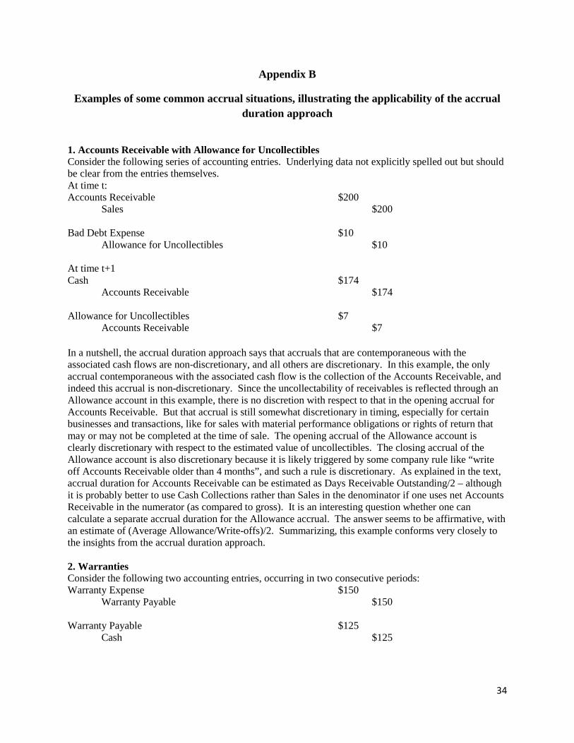
1. Accounts Receivable with Allowance for Uncollectibles Consider the following series of accounting entries. Underlying data not explicitly spelled out but should be clear from the entries themselves. At time t: Accounts Receivable $200 Sales $200 Bad Debt Expense $10 Allowance for Uncollectibles $10 At time t+1 Cash $174 Accounts Receivable $174 Allowance for Uncollectibles $7 Accounts Receivable $7 In a nutshell, the accrual duration approach says that accruals that are contemporaneous with the associated cash flows are non-discretionary, and all others are discretionary. In this example, the only accrual contemporaneous with the associated cash flow is the collection of the Accounts Receivable, and indeed this accrual is non-discretionary. Since the uncollectability of receivables is reflected through an Allowance account in this example, there is no discretion with respect to that in the opening accrual for Accounts Receivable. But that accrual is still somewhat discretionary in timing, especially for certain businesses and transactions, like for sales with material performance obligations or rights of return that may or may not be completed at the time of sale. The opening accrual of the Allowance account is clearly discretionary with respect to the estimated value of uncollectibles. The closing accrual of the Allowance account is also discretionary because it is likely triggered by some company rule like “write off Accounts Receivable older than 4 months”, and such a rule is discretionary. As explained in the text, accrual duration for Accounts Receivable can be estimated as Days Receivable Outstanding/2 – although it is probably better to use Cash Collections rather than Sales in the denominator if one uses net Accounts Receivable in the numerator (as compared to gross). It is an interesting question whether one can calculate a separate accrual duration for the Allowance accrual. The answer seems to be affirmative, with an estimate of (Average Allowance/Write-offs)/2. Summarizing, this example conforms very closely to the insights from the accrual duration approach. 2. Warranties Consider the following two accounting entries, occurring in two consecutive periods: Warranty Expense $150 Warranty Payable $150 Warranty Payable $125 Cash $125

35

This example is a straightforward application of the accrual duration approach. The opening accrual for warranty payable is discretionary because it is an estimate of future warranty claims. The closing accrual is non-discretionary because it is pinned down by the amount of warranty claims paid out. The average duration of the Warranty Payable account for a given period can be estimated as (Average Warranty Payable/Cash Paid out for Warranties)/2, and it is clear that discretion in recording Warranty Payable increases in the duration of this accrual. If the business is simple, the duration of the Warranty Payable can also be potentially estimated from specific disclosure about warranty coverage. For example, for a company that produces only watches with warranty of 2 years, assuming warranty claims are even throughout warranty life implies an average duration of Warranty Payable of 1 year. 3. Prepaid Rent Prepaid Rent $100 Cash $100 Rent Expense $24 Prepaid Rent $24 The opening entry is clearly non-discretionary. The closing entry is often not really discretionary for a simple case with constant monthly rent, for example. But rent expense can be discretionary as well in cases where rent expense is tied to sales volumes, and thus quarterly rent expense assumes projections about annual sales. It can be also discretionary in cases where there is an accrual for projected rental penalties specified in the rental contract. The accrual duration for Prepaid Rent is calculated as (Average Prepaid Rent/Rent Expense)/2. 4. Deferred Revenue Cash $800 Deferred Revenue $800 Deferred Revenue $475 Sales Revenue $475 The opening entry is a non-discretionary deferral of cash received until delivery of goods or services. Depending on the type of good or service provided, the closing entry can be quite discretionary, especially for contracts with complicated performance obligations, multiple deliverables, rights-of-return, etc. The accrual duration for Deferred Revenue is (Average Deferred Revenue/Sales Revenue)/2.

36

References:

Altamuro, Jennifer, Anne L. Beatty, and Joseph Weber, 2005, The effects of accelerated revenue recognition on earnings management and earnings informativeness: Evidence from SEC Staff Accounting Bulletin No. 101, The Accounting Review 80 (2), 373-401.

Ball, Ray, 2013, Accounting informs investors and earnings management is rife: two questionable beliefs, Accounting Horizons 27 (4), 847-853.

Ball, Ray, and Lakshmanan Shivakumar, 2006, The role of accruals in asymmetrically timely gain and loss recognition, Journal of Accounting Research 44 (2), 207-242.

Beaver, William H., and Maureen F. McNichols, 1998, The characteristics and valuation of loss reserves of property casualty insurers, Review of Accounting Studies 3 (1-2), 73-95.

Bushman, Robert M., Alina Lerman, and X. Frank Zhang, 2016, The changing landscape of accrual accounting, Journal of Accounting Research 54 (1), 41-78.

Chan, Louis K.C., Jason Karsecki, and Josef Lakonishok, 2003, The level and persistence of growth rates, The Journal of Finance 58 (2), 643-684.

Dechow, Patricia M., 1994, Accounting earnings and cash flows as measures of firm performance: The role of accounting accruals, Journal of Accounting and Economics 18, 3-42.

Dechow, Patricia M., and Ilia D. Dichev, 2002, The quality of accruals and earnings: the role of accrual estimation errors, The Accounting Review 77 (S-1), 35-59.

Dechow, Patricia M., Weili Ge, Chad R. Larson, Richard G. Sloan, 2011, Predicting material accounting misstatements, Contemporary Accounting Research 28 (1), 17-82.

Dechow, Patricia, Weili Ge, and Catherine Schrand, 2010, Understanding earnings quality: A review of the proxies, their determinants and their consequences, Journal of Accounting and Economics 50, 344-401.

Dechow, Patricia M., S.P. Kothari, and Ross L. Watts, 1998, The relation between earnings and cash flows, Journal of Accounting and Economics 25, 131-214.

Dechow, Patricia M., Richard G. Sloan, and Amy P. Sweeney, 1995, Detecting earnings management, The Accounting Review 70 (2), 193-225.

Dichev, Ilia D., John R. Graham, Campbell R. Harvey, and Siva Rajgopal, 2013, Earnings quality: Evidence from the field, Journal of Accounting and Economics 56, 1-33.

Francis, Jennifer, Ryan LaFond, Per Olsson, and Katherine Schipper, 2005, The market pricing of accruals quality, Journal of Accounting and Economics 39 (2), 295-327.

Francis, Jennifer, Per Olsson, and Katherine Schipper, 2008, Earnings quality, Now Publishers Inc. Jones, Jennifer, 1991, Earnings management during import relief investigations, Journal of Accounting

Research 29 (2), 193-228. Leuz, Christian, Dhananjay Nanda, and Peter Wysocki, Earnings management and investor protection: an

international comparison, Journal of Financial Economics 69 (3), 505-527. Peterson, Kyle, 2011, Accounting complexity, misreporting, and the consequences of misreporting,

Review of Accounting Studies 17 (1), 72-95. Petroni, Kathy Ruby, 1992, Optimistic reporting in the property-casualty insurance industry, Journal of

Accounting and Economics 15 (4) 485-508. Richardson, Scott A., Richard G. Sloan, Mark T. Soliman, and Irem Tuna, 2005, Accrual reliability,

earnings persistence, and stock prices, Journal of Accounting and Economics 39 (3), 437-485. Sloan, Richard G., 1996, Do stock prices fully reflect information in accruals and cash flows about future

earnings?, The Accounting Review 71 (3), 289-315. White, Hal, 2012, Accruals, deferrals, cash flows, and earnings: Articulation implications for earnings

management models and a suggested alternative, Working paper, Penn State University, also available on ssrn.com.

37

Figure 1 Schematic representation of the benefits and costs of the accrual process as reflected in the

timing of accruals and income

Definitions: Cash flow accounting: Cash inflows are revenues and income, cash outflows are expenses and losses Actual accrual accounting: Income = Cash flows + Accruals; accruals are recorded using real-time

forward-looking estimates Perfect foresight accounting: Income = Cash flows + Accruals; accruals are recorded under perfect

foresight Maximum potential benefits from using accrual accounting: Difference between Cash flow accounting

and Perfect foresight accounting” Costs of using accrual accounting: Making timing errors in income, which are the difference between

actual recorded income and income under perfect foresight Net benefits of using accrual accounting: Difference between Cash flow accounting and Actual accrual

accounting; More timely recognition of income at the cost of making timing errors

Cash flow accounting Actual accrual accounting Perfect foresight accounting

Net benefits from using accrual accounting Cost of using accruals: Timing errors

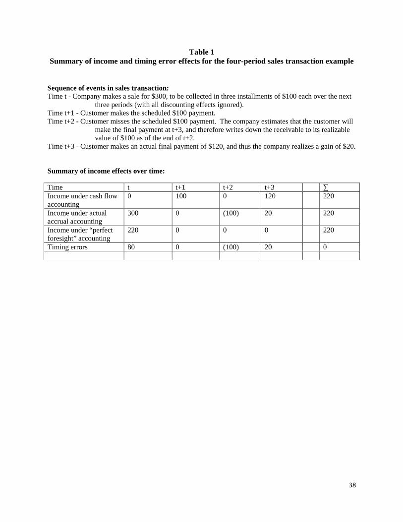
38

Table 1 Summary of income and timing error effects for the four-period sales transaction example

Sequence of events in sales transaction: Time t - Company makes a sale for $300, to be collected in three installments of $100 each over the next

three periods (with all discounting effects ignored). Time t+1 - Customer makes the scheduled $100 payment. Time t+2 - Customer misses the scheduled $100 payment. The company estimates that the customer will

make the final payment at t+3, and therefore writes down the receivable to its realizable value of $100 as of the end of t+2.

Time t+3 - Customer makes an actual final payment of $120, and thus the company realizes a gain of $20.

Summary of income effects over time:

Time t t+1 t+2 t+3 ∑ Income under cash flow accounting

0 100 0 120 220

Income under actual accrual accounting

300 0 (100) 20 220

Income under “perfect foresight” accounting

220 0 0 0 220

Timing errors 80 0 (100) 20 0