Embed Size (px)
Citation preview

Accounting Research Center, Booth School of Business, University of Chicago
Fundamental Information AnalysisAuthor(s): Baruch Lev and S. Ramu ThiagarajanSource: Journal of Accounting Research, Vol. 31, No. 2 (Autumn, 1993), pp. 190-215Published by: Blackwell Publishing on behalf of Accounting Research Center, Booth School ofBusiness, University of ChicagoStable URL: http://www.jstor.org/stable/2491270Accessed: 26/05/2010 02:22
Your use of the JSTOR archive indicates your acceptance of JSTOR's Terms and Conditions of Use, available athttp://www.jstor.org/page/info/about/policies/terms.jsp. JSTOR's Terms and Conditions of Use provides, in part, that unlessyou have obtained prior permission, you may not download an entire issue of a journal or multiple copies of articles, and youmay use content in the JSTOR archive only for your personal, non-commercial use.
Please contact the publisher regarding any further use of this work. Publisher contact information may be obtained athttp://www.jstor.org/action/showPublisher?publisherCode=black.
Each copy of any part of a JSTOR transmission must contain the same copyright notice that appears on the screen or printedpage of such transmission.
JSTOR is a not-for-profit service that helps scholars, researchers, and students discover, use, and build upon a wide range ofcontent in a trusted digital archive. We use information technology and tools to increase productivity and facilitate new formsof scholarship. For more information about JSTOR, please contact [email protected].
Accounting Research Center, Booth School of Business, University of Chicago and Blackwell Publishing arecollaborating with JSTOR to digitize, preserve and extend access to Journal of Accounting Research.
http://www.jstor.org
Journal of Accounting Research Vol. 31 No. 2 Autumn 1993
Printed in US.A.
Fundamental Information Analysis
BARUCH LEV* AND S. RAMU THIAGARAJANt
1. Introduction
Fundamental analysis is aimed at determining the value of corporate securities by a careful examination of key value-drivers, such as earn- ings, risk, growth, and competitive position. In the context of such anal- ysis, we identify below a set of financial variables (fundamentals) claimed by analysts to be useful in security valuation and examine these claims by estimating the incremental value-relevance of these variables over earnings. Our findings support the incremental value-relevance of most of the identified fundamentals; in fact, for the 1980s, the fundamentals add approximately 70%, on average, to the explanatory power of earn- ings with respect to excess returns. We also show that the returns-fun- damentals relation is considerably strengthened when it is conditioned on macroeconomic variables, thereby demonstrating the importance of a contextual capital market analysis. For example, several fundamentals that appear only weakly value-relevant or even irrelevant in the uncon- ditional analysis exhibit strong association with returns under specific economic conditions (e.g., the accounts receivable and the provision for doubtful receivables signals during high inflation).
From a general examination of the role of fundamentals in security valuation we turn to the related issues of earnings persistence, growth, and the earnings response coefficient. We hypothesize that the funda-
*Un7iversity of California, Berkeley; tNorthwestern University. The helpful comments of Jeffery Abarbanell, Ray Ball, Linda Bamber, Brad Barber, Maiy Barth, William Beaver, Victor Bernard, Gaiy Biddle, Robert Bowen, Nicholas Dopuch, Catherine Finger, George Foster, Robert Freeman, Robert Kaplan, Charles Lee, Krishna Palepu, Stephen Penman, K. Ramesh, Terry Shevlin, Toshi Shibano, D. Shores, Abbie Smith, Jacob Thomas, Brett Trueman, Ross Watts, Greg Waymire, Roman Weil, and Paul Zarowin are gratefully acknowledged.
190
Copyright ?, Institute of Professional Accounting 1993
FUNDAMENTAL INFORMATION ANALYSIS 191
mental signals identified in this study are used by investors to assess the persistence (sometimes referred to as "quality") and growth of reported earnings. We provide support for this hypothesis by demonstrating a significant relation between an aggregate score reflecting the information in the fundamentals and two indicators of persistence: the earnings re- sponse coefficient and future earnings growth. In fact, this fundamental ("quality of earnings") score is more strongly associated with the response coefficient than a time-series-based persistence measure, suggesting that the former is more effective in capturing the permanent component of earnings than the latter, which is commonly used by researchers.
We identify candidate fundamentals to be included in the empirical tests from the written pronouncements of financial analysts. This guided search procedure is different from the statistical search used in previous research, such as Ou and Penman [1989]. A directed search for fundamentals, guided by theory or by experts' judgment, is a natu- ral extension of the statistical search procedure.1
This study thus extends the search for value-relevant fundamentals both by using a guided choice of candidate variables and by condition- ing the returns-fundamentals relation on macroeconomic variables (a contextual analysis). We also link our fundamental analysis findings with the persistence/response coefficient literature by demonstrating that the identified fundamentals capture important characteristics of earnings persistence.
2. The Search for Fundamentals
To identify a set of fundamentals used to evaluate firms' performance and estimate future earnings, we searched the Wall Street Journal and Barron's for 1984-90;2 Value Line publications on "quality of earnings" [1973a; 1973b]; professional commentaries on corporate financial re- porting and analysis, such as the Quality of Earnings publications;3 and newsletters of major securities firms commenting on the value-relevance of financial information.
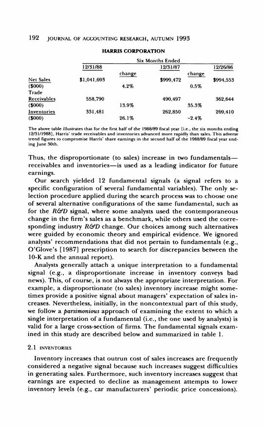
The following example, from the Quality of Earnings Report on Harris Corporation (March 27, 1989), illustrates how analysts use fundamentals to draw inferences about the firm's current performance and its future earnings:
1 A guided search for fundamentals also yields variables that can be intuitively moti- vated to students and practitioners, while a statistical search might identify unknown and hard-to-justify variables (e.g., Ou and Penman's Sales to Total Cash ratio or Holthausen and Larcker's [1992] Percent Change in Sales over Total Assets ratio), which probably proxy for other underlying constructs.
2 The key phrases used for search in the Dow Jones News Service Text data base were "Quality of Earnings" and "Quality of Assets."
3 Published by the Reporting Research Corporation, Englewood Cliffs, N. J. See also the book by this firm's CEO, Thornton O'Glove, Quality of Earnings [1987]. A similar commentary is provided by Mr. David Tice in his newsletter, Behind the Numbers.
192 JOURNAL OF ACCOUNTING RESEARCH, AUTUMN 1993
HARRIS CORPORATION
Six Months Ended
12/31/88 12/31/87 12/26/86
change change
Net Sales $1,041,693 $999,472 $994,553
($000) 4.2% 0.5%
Trade
Receivables 558,790 490,497 362,644
($000) 13.9% 35.3%
Inventories 331,481 262,850 269,410
($000) 26.1% -2.4%
The above table illustrates that for the first half of the 1988/89 fiscal year [i.e., the six months ending 12/31/1988], Harris' trade receivables and inventories advanced more rapidly than sales. This adverse trend figures to compromise Harris' share earnings in the second half of the 1988/89 fiscal year end- ing June 30th.
Thus, the disproportionate (to sales) increase in two fundamentals- receivables and inventories-is used as a leading indicator for future earnings.
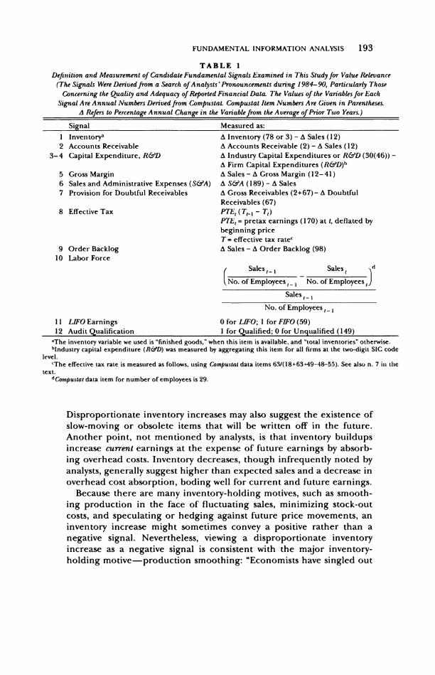
Our search yielded 12 fundamental signals (a signal refers to a specific configuration of several fundamental variables). The only se- lection procedure applied during the search process was to choose one of several alternative configurations of the same fundamental, such as for the R&D signal, where some analysts used the contemporaneous change in the firm's sales as a benchmark, while others used the corre- sponding industry R&D change. Our choices among such alternatives were guided by economic theory and empirical evidence. We ignored analysts' recommendations that did not pertain to fundamentals (e.g., O'Glove's [1987] prescription to search for discrepancies between the 10-K and the annual report).
Analysts generally attach a unique interpretation to a fundamental signal (e.g., a disproportionate increase in inventory conveys bad news). This, of course, is not always the appropriate interpretation. For example, a disproportionate (to sales) inventory increase might some- times provide a positive signal about managers' expectation of sales in- creases. Nevertheless, initially, in the noncontextual part of this study, we follow a parsimonious approach of examining the extent to which a single interpretation of a fundamental (i.e., the one used by analysts) is valid for a large cross-section of firms. The fundamental signals exam- ined in this study are described below and summarized in table 1.
2.1 INVENTORIES
Inventory increases that outrun cost of sales increases are frequently considered a negative signal because such increases suggest difficulties in generating sales. Furthermore, such inventory increases suggest that earnings are expected to decline as management attempts to lower inventory levels (e.g., car manufacturers' periodic price concessions).
FUNDAMENTAL INFORMATION ANALYSIS 193
TABLE 1 Definition and Measurement of Candidate Fundamental Signals Examined in This Study for Value Relevance
(The Signals Were Derived from a Search of Analysts' Pronouncements during 1984-90, Particularly Those Concerning the Quality and Adequacy of Reported Financial Data. The Values of the Variables for Each
Signal Are Annual Numbers Derived from Compustat. Compustat Item Numbers Are Given in Parentheses. A Refers to Percentage Annual Change in the Variable from the Average of Prior Two Years.)
Signal Measured as:
1 Inventorya A Inventory (78 or 3) - A Sales (12) 2 Accounts Receivable A Accounts Receivable (2) - A Sales (12)
3-4 Capital Expenditure, R&D A Industry Capital Expenditures or R&D (30(46)) - A Firm Capital Expenditures (R&D)b
5 Gross Margin A Sales - A Gross Margin (12-41) 6 Sales and Administrative Expenses (S&A) A S&A (189) - A Sales 7 Provision for Doubtful Receivables A Gross Receivables (2+67)- A Doubtful
Receivables (67) 8 Effective Tax PTE, (T 1i - TO)
PTE1 = pretax earnings (170) at t, deflated by beginning price T= effective tax ratec
9 Order Backlog A Sales - A Order Backlog (98) 10 Labor Force
Sales1o1 Sales d
No. of Employees, -- No. of Employees t)
Sales , I
No. of Employees t-
11 LIFO Earnings 0 for LIFO; 1 for FIFO (59) 12 Audit Qualification 1 for Qualified; 0 for Unqualified (149)
aThe inventory variable we used is "finished goods," when this item is available, and "total inventories" otherwise. bIndustry capital expenditure (R&D) was measured by aggregating this item for all firms at the two-digit SIC code
level. cThe effective tax rate is measured as follows, using Compustat data items 63/(18+63+49-48-55). See also n. 7 in the
text. dConipustat data item for number of employees is 29.
Disproportionate inventory increases may also suggest the existence of slow-moving or obsolete items that will be written off in the future. Another point, not mentioned by analysts, is that inventory buildups increase current earnings at the expense of future earnings by absorb- ing overhead costs. Inventory decreases, though infrequently noted by analysts, generally suggest higher than expected sales and a decrease in overhead cost absorption, boding well for current and future earnings.
Because there are many inventory-holding motives, such as smooth- ing production in the face of fluctuating sales, minimizing stock-out costs, and speculating or hedging against future price movements, an inventory increase might sometimes convey a positive rather than a negative signal. Nevertheless, viewing a disproportionate inventory increase as a negative signal is consistent with the major inventory- holding motive-production smoothing: "Economists have singled out
194 BARUCH LEV AND S. RAMU THIAGARAJAN
the production-smoothing/buffer-stock motive for attention" (Blinder and Maccini [1991, p. 78]).
When production varies less than sales, a disproportionate inventory increase may result from an unexpected sales decrease, loss of produc- tion or inventory control, or growth of obsolete inventory items-all reflecting negatively on future earnings. Since these arguments apply particularly to the "finished goods" component of inventory, our em- pirical tests are based on this component when it is available on Com-
pustat, and on "total inventories" otherwise. We computed for each sample firm and year the following inventory
signal:
Percentage Change in Inventory - Percentage Change in Sales.4 (1)
The annual percentage change in inventory (and correspondingly for sales) is defined as:
[Inventoryt - E(Inventoryt)] / E(Inventoryt), (2)
where E(.) denotes expected value. Since we regress unexpected returns on the fundamental signals, the signals should reflect the unexpected component of the fundamental variable. We used two expectation models: a random walk and a two-year averaging model (E(Inventoryt) = 1/2(Inventoryt-1 + Inventoryt-2)). The empirical tests indicated that the two expectation models yield very similar results; the findings re- ported below are those based on the two-year average model for all the fundamental signals. Since a positive value of the inventory signal is a priori perceived as "bad news," the signal is expected to be negatively correlated with stock returns.
2.2 ACCOUNTS RECEIVABLE
Disproportionate (to sales) increases in accounts receivable are men- tioned by analysts as conveying a negative signal almost as often as in-
ventory increases. Disproportionate accounts receivable increases may suggest difficulties in selling the firm's products (generally triggering credit extensions), as well as an increasing likelihood of future earn- ings decreases from increases in receivables' provisions. A dispropor- tionate receivables increase might also suggest earnings manipulation, as yet unrealized revenues are recorded as sales. These underlying rea- sons for receivables increases indicate low persistence of current earn- ings and future earnings decreases. The accounts receivable signal was measured similarly to the inventory signal (1).
4Strictly speaking, the benchmark in expression (1) should be cost of sales. Empiri- cally, the two benchmarks yielded virtually identical results. The sales benchmark was preferred because it is consistent with the signals suggested by analysts.
FUNDAMENTAL INFORMATION ANALYSIS 195
2.3 CAPITAL EXPENDITURES
2.4 R&D
Relative decreases in capital expenditures and R&D intensities are often perceived negatively by analysts. The largely discretionary nature of these expenditures makes disproportionate decreases a priori sus- pect. A decrease in capital expenditures may indicate managers' con- cerns with the adequacy of current and future cash flows to sustain the previous investment level. Similarly, a cut in R&D may indicate man- agement's concern about the adequacy of reported earnings and sug- gest attempts to boost earnings by decreasing R&D expenses. In general, capital expenditures and R&D decreases are equated by ana- lysts with a short-term managerial orientation, while increases in these items appear to bode well for future earnings and cash flows.
Unlike the preceding inventory and accounts receivable cases, the theoretical relation between capital expenditures (or R&D) and sales is tenuous. For example, recent research (e.g., Fazzari, Hubbard, and Peterson [1988]) suggests that liquidity position and cash flow are stronger determinants of investment (capital expenditure, R&D) deci- sions than are current sales. Absent a clear theoretical guidance, we used an industry benchmark for the capital expenditures and R&D in- novations (signals), defining them as the annual percentage change in total two-digit industry capital expenditures (or R&D) minus the an- nual percentage change in the corresponding firm's items.5 As with other signals, the measures were defined to yield an expected negative response coefficient with stock returns: a positive value of the two sig- nals (i.e., industry growth larger than the firm's) implies, a priori, bad news, and therefore a negative relation with returns.
2.5 GROSS MARGIN
A disproportionate (to sales) decrease in the gross margin balance (sales minus cost of sales) is viewed negatively by analysts (e.g., Graham et al. [1962, p. 244] and Hawkins [1986]). Gross margin is, in general, a less noisy indicator than earnings of the relation between the firm's input and output prices. This relation is driven by underlying factors, such as intensity of competition and the relation between fixed and variable expenses (operating leverage). Variations in these fundamen- tal factors (indicated by disproportionate changes in gross margin) ob- viously affect the long-term performance of the firm and are therefore informative with respect to earnings persistence and firm values. The gross margin signal was defined as the difference between the percent- age change in sales and that of the gross margin.
5Both analysts and researchers often compare a given firm's R&D and capital expen- diture levels to those of similar firms within the industry. For example, see the Wall Street Journal (September 17, 1990, p. C2) on Digital Equipment Corp. and Grabowski [1978].
196 BARUCH LEV AND S. RAMU THIAGARAJAN
2.6 SELLING AND ADMINISTRATIVE (S&A) EXPENSES
Most administrative costs are approximately fixed, therefore, a dis- proportionate (to sales) increase is considered a negative signal sug- gesting, among other things, a loss of managerial cost control or an unusual sales effort (Bernstein [1988, p. 692]). This signal was defined as the difference between the annual percentage change in S&A ex- penses and the percentage change of sales.
2.7 PROVISION FOR DOUBTFUL RECEIVABLES
This provision is largely discretionary, so unusual changes (relative to accounts receivable) are generally suspect by analysts (McNichols and Wilson [1988] and O'Glove [1987, p. 83]). Firms with inadequate provisions for doubtful receivables are expected to suffer future earn- ings decreases from provision increases. Our sources frequently re- ferred to the adverse implications of inadequate bad debt provisions (in recent years particularly for loan losses of financial companies) for the persistence and growth of earnings.
The provision for doubtful receivables signal was measured relative to the change in gross accounts receivable:
Percentage Change in Gross - Percentage Change in Provision (3) Accounts Receivable for Doubtful Receivables.
Positive values of this measure are perceived as a negative signal. How- ever, there may be cases where the credit-worthiness of customers im- proved, on average, and a decrease in the relative level of the provision was warranted. As noted earlier, we follow in the first (noncontextual) part of this study the modus operandi of analysts and attach a single in- terpretation to a fundamental signal.
2.8 EFFECTIVE TAX RATE
A significant change in the firm's effective tax rate which is not caused by a statutory tax change is generally considered transitory by analysts (see, e.g., a Wall StreetJournal [January 26, 1990] story on Lo- tus Development Corporation). Accordingly, an unusual decrease in the effective tax rate is generally considered a negative signal about earnings persistence.
To focus on the impact of the effective tax rate change on earnings, we decomposed the annual change in earnings, AEt = Et- Et-,, into two components: (a) the change in pretax earnings (APTEt), at last year's effective tax (Tt-1) level-APTEt(1 - Tt-1), and (b) the effect of the tax rate change on current pretax earnings-PTEt(Tt_1 - Tt):
AEt = APTEt(I - Tt-1) + PTEt(Tt-I - Tt). (4)
In expression (4), PTEt(Tt-I - Tt), which indicates the part of the net earnings change due to the effective tax rate change, is our measure of
FUNDAMENTAL INFORMATION ANALYSIS 197
the tax signal (after deflation by beginning price).6 The effective tax rate was measured as the current federal tax expense divided by pretax earnings (minus equity income from unconsolidated subsidiaries plus income from minority interests).7
2.9 ORDER BACKLOG
This leading indicator of future sales and earnings is generally defined as the dollar amount of firm unfilled orders at year-end. Changes in order backlog relative to the level of operations are fre- quently used by analysts to indicate future performance, particularly in the high technology and heavy industries (e.g., software, semiconduc- tors, steel and aircraft manufacturers).8 In addition to indicating genu- ine changes in the demand for the firm's products, a relative (to sales) decrease in order backlog may suggest that yet unrealized sales were recorded in the current period, an "earnings management" procedure prevalent among high-tech companies (see the Treadway Commission Report [1987]). The order backlog signal was defined as the difference between the percentage change in sales and that of order backlog.
2.10 LABOR FORCE
Financial analysts generally comment favorably on announcements of corporate restructuring, particularly labor force reductions. This pro- vides yet another example of analysts' use of fundamental signals to estimate the persistence of earnings, since in the year of a significant la- bor force reduction wage-related expenses (e.g., severance pay) gener- ally increase.9 Reported earnings, in such cases, do not reflect the future benefits from restructuring, and fundamentals, such as the labor force signal, are used to provide a better assessment of future earnings.
6A simple hypothetical example will provide intuition to this measure. Assume:
Period: t t- 1 Earnings before tax 120 100 Effective tax rate 0.25 0.40 Net earnings 90 60
The net earnings change, 30, consists according to (4) of the before tax earnings change, 20 x 0.60 = 12, and the impact of the tax rate change, 120 (0.40 - 0.25) = 18. The latter (price-deflated) component of the total earnings change is our tax signal.
7This measure is used by Porcano [1986] and examined in Omer, Molloy, and Ziebart [1991]. Compustat item numbers for this measure are 63 / (18 + 63 + 49- 48 - 55). Firms having both a negative numerator and a negative denominator were excluded from the sample. Following Omer, Molloy, and Ziebart [1991], firms with a positive numerator and negative denominator were coded to represent the statutary rate (48% before 1986, 46% in 1986, and 34% starting in 1987).
8The relative (to sales) change in order backlog is, for example, the measure most closely watched in the computer (particularly semiconductor) industry, where it is known as the "Book to Bill" ratio, relating order backlog (Book) to sales (Bill).
9 For example, Exxon laid off almost 40% of its work force in 1986, yet total wages and salaries increased that year by 3%.
198 BARUCH LEV AND S. RAMU THIAGARAJAN
We defined the labor force signal as the annual percentage change in sales-per-employee (the ratio of annual sales to the number of em- ployees at year-end). Scaling sales by the number of employees is aimed at both capturing changes in the efficiency of labor and ac- counting for changes in the number of employees. As before, this vari- able is defined to yield an expected negative coefficient sign.
2.11 LIFO EARNINGS
When input prices are increasing, LIFO earnings are regarded as more sustainable or closer to "economic earnings" than EIFO earnings, since LIFO cost-of-sales is a closer proxy to current (replacement) cost than FIFO cost-of-sales (see Hawkins [1986, p. 208] and Bernstein [1988, p. 147]). The use of the LIFO inventory method is, therefore, considered a positive signal, depicted here by a dummy variable: 0 for LIFO or replacement cost, and 1 for FIFO, average cost, or other inven- tory methods.10 Although LIFO valuation subsequent to the adoption year is not unexpected by investors, we wished to examine whether its mere use commands higher returns.
2.12 AUDIT QUALIFICATION
A qualified, disclaimed, or adverse audit opinion obviously sends a negative message to investors. To capture this signal we used a dummy variable: 1 if the auditor's opinion was qualified or adverse, and 0 for an unqualified opinion.
3. Methodology, Sample Selection, and Findings
To examine empirically the incremental value-relevance over earnings of our 12 candidate fundamentals, we ran the following two cross- sectional regressions. First, the conventional returns-earnings regression:
Ri = a + bAEj + uj; i = 1,2,. .. ,n, number of firms (5)
where:
Ri= 12 months excess stock return of firm i, where the return cumulation starts with the fourth month after the beginning of the fiscal year. The excess return is determined by sub- tracting from the realized return the "market model" ex- pected return.11
10 We also experimented with a "slope dummy," multiplying the LIFO-FIFO dummy by the earnings change. This variable, however, had a very high correlation with the earn- ings change variable (over 0.90), yielding statistically insignificant estimates. Carroll, Col- lins, and Johnson [1991] examine such a slope effect and find the response coefficient of LIFO firms to be higher than that of FIFO firms.
11 The "market model" a and P coefficients used to derive the expected returns were estimated using a value-weighted index from 36 monthly returns ending with the sixth
FUNDAMENTAL INFORMATION ANALYSIS 199
AEi = the annual change in EPS (primary, excluding extraordi- nary items), deflated by beginning-of-year share price.
The second regression includes the fundamentals:
12
Ri = a + boAPTEi + 2 bjSji + vi (6) j-1 Ip z
APTEi = the annual change in pretax earnings times one minus last year's effective tax rate. This is the first component on the right side of expression (4); the second component is the tax signal. The sum of these two components is AEi.
S.i = fundamental signals outlined in table 1; j= 1,... ,12.
Expression (5) is used as a benchmark against which expression (6) is evaluated. Sample firms were selected by the following criteria:
(i) Availability of "primary earnings per-share excluding extraordi- nary items" data on the Compustat tape (item #58) and data re- quired for the fundamental signals (see table 1), for the sample period, 1970-88.
(ii) Availability on the CRSP tape of monthly stock returns starting at least 36 months prior to the return cumulation period for year "t." (All relevant variables were adjusted for stock splits and stock dividends. Firms which changed fiscal years during the sample period were eliminated.)
Table 2 presents OLS estimates of the 1974-88 year-by-year cross- sectional regressions (5) and (6) and an across-years significance test.12 Table 2 estimates are for firms having data for all 12 fundamental sig- nals (roughly 140-180 firms per year). This restricted sample is not representative; for example, it includes only companies with R&D ex- penditures. In table 3 we report estimates from a much larger sample, roughly 500-600 firms per year, where the data requirements for R&D, Provision for Doubtful Receivables, and Order Backlog were re- moved. These three fundamentals caused the largest loss of firms in the restricted sample (e.g., Order Backlog was reported by only 35% of the sample firms). This larger sample is quite representative, including
month of the preceding fiscal year. Some sample firms (less than 5% of total sample) had less than 36 monthly returns. The minimum number of returns used for these firms was 10. The resulting monthly returns were compounded to obtain annual returns.
12 Given some extreme values of the fundamental signals, mainly due to small denom- inators in the percentage change computation, we eliminated the extreme 1% of each fundamental signal. Analysis of the regression residuals indicated existence of some out- liers. Based on an analysis of studentized residual (greater than 3) and Cook's D statistic (greater than 1), these were removed. To examine the sensitivity of our findings to this elimination, we reran regressions (5) and (6) on the original (nontruncated) data and found that the elimination marginally increased the significance of some coefficients. However, none of our conclusions depends on the elimination.
200 BARUCH LEV AND S. RAMU THIAGARAJAN
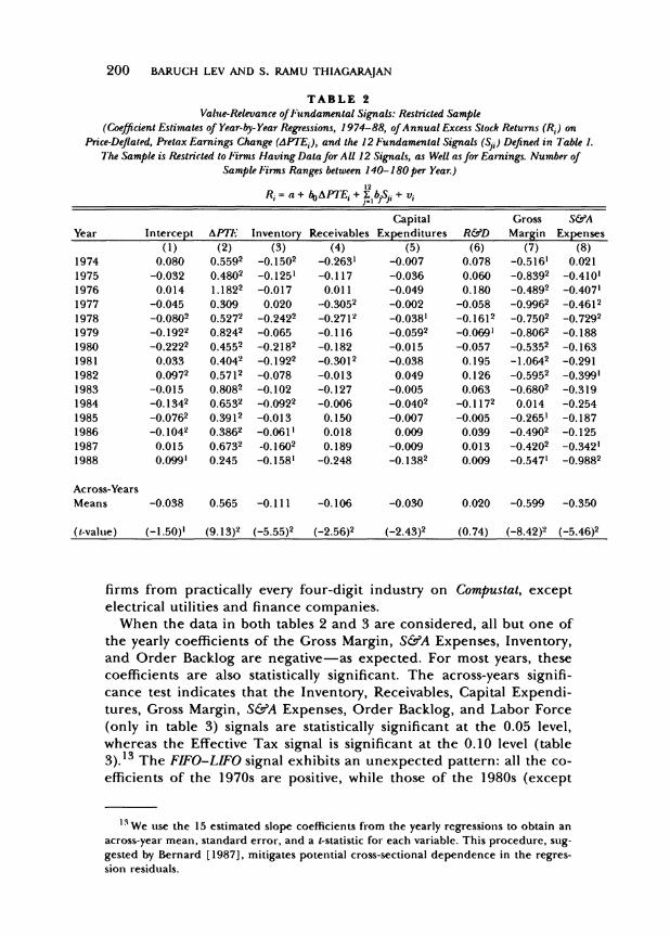
TABLE 2 Value-Relevance of Fundamental Signals: Restricted Sample
(Coefficient Estimates of Year-by- Year Regressions, 1974-88, of Annual Excess Stock Returns (Rd) on Price-Deflated, Pretax Earnings Change (APTEd), and the 12 Fundamental Signals (Sjf) Defined in Table 1.
The Sample is Restricted to Firms Having Data for All 12 Signals, as Well as for Earnings. Number of Sample Firms Ranges between 140-180 per Year.)
12 Ri = a + boAPTE, + X_ bjSji + Vi
Capital Gross S&A Year Intercept APTE Inventory Receivables Expenditures R&D Margin Expenses
(1) (2) (3) (4) (5) (6) (7) (8) 1974 0.080 0.5592 -0.1502 -0.2631 -0.007 0.078 -0.516' 0.021 1975 -0.032 0.4802 -0.1251 -0.117 -0.036 0.060 -0.8392 -0.410' 1976 0.014 1.1822 -0.017 0.011 -0.049 0.180 -0.4892 -0.4071 1977 -0.045 0.309 0.020 -0.3052 -0.002 -0.058 -0.9962 -0.4612 1978 -0.0802 0.5272 -0.2422 -0.2712 -0.038' -0.1612 -0.75 02 -0.7292 1979 -0.1922 0.8242 -0.065 -0.116 -0.0592 -0.0691 -0.8062 -0.188 1980 -0.2222 0.4552 -0.2182 -0.182 -0.015 -0.057 -0.5352 -0.163 1981 0.033 0.4042 -0.1922 -0.3012 -0.038 0.195 -1.0642 -0.291
1982 0.0972 0.5712 -0.078 -0.013 0.049 0.126 -0.5952 -0.3991 1983 -0.015 0.8082 -0.102 -0.127 -0.005 0.063 -0.6802 -0.319 1984 -0.1342 0.6532 -0.0922 -0.006 -0.0402 -0.1172 0.014 -0.254 1985 -0.0762 0.3912 -0.013 0.150 -0.007 -0.005 -0.265' -0.187 1986 -0.1042 0.3862 -0.061' 0.018 0.009 0.039 -0.4902 -0.125 1987 0.015 0.6732 -0.1602 0.189 -0.009 0.013 -0.4202 -0.342' 1988 0.099' 0.245 -0.158' -0.248 -0.1382 0.009 -0.5471 -0.9882
Across-Years Means -0.038 0.565 -0.111 -0.106 -0.030 0.020 -0.599 -0.350
(t-value) (-1.50)1 (9.13)2 (-5.55)2 (-2.56)2 (-2.43)2 (0.74) (-8.42)2 (-5.46)2
firms from practically every four-digit industry on Compustat, except electrical utilities and finance companies.
When the data in both tables 2 and 3 are considered, all but one of the yearly coefficients of the Gross Margin, S&A Expenses, Inventory, and Order Backlog are negative-as expected. For most years, these coefficients are also statistically significant. The across-years signifi- cance test indicates that the Inventory, Receivables, Capital Expendi- tures, Gross Margin, S&A Expenses, Order Backlog, and Labor Force (only in table 3) signals are statistically significant at the 0.05 level, whereas the Effective Tax signal is significant at the 0.10 level (table 3).13 The FIFO-LIFO signal exhibits an unexpected pattern: all the co- efficients of the 1970s are positive, while those of the 1980s (except
13We use the 15 estimated slope coefficients from the yearly regressions to obtain an across-year mean, standard error, and a t-statistic for each variable. This procedure, Sug- gested by Bernard [1987], mitigates potential cross-sectional dependence in the regres- sion residuals.
FUNDAMENTAL INFORMATION ANALYSIS 201
T A B L E 2-continued
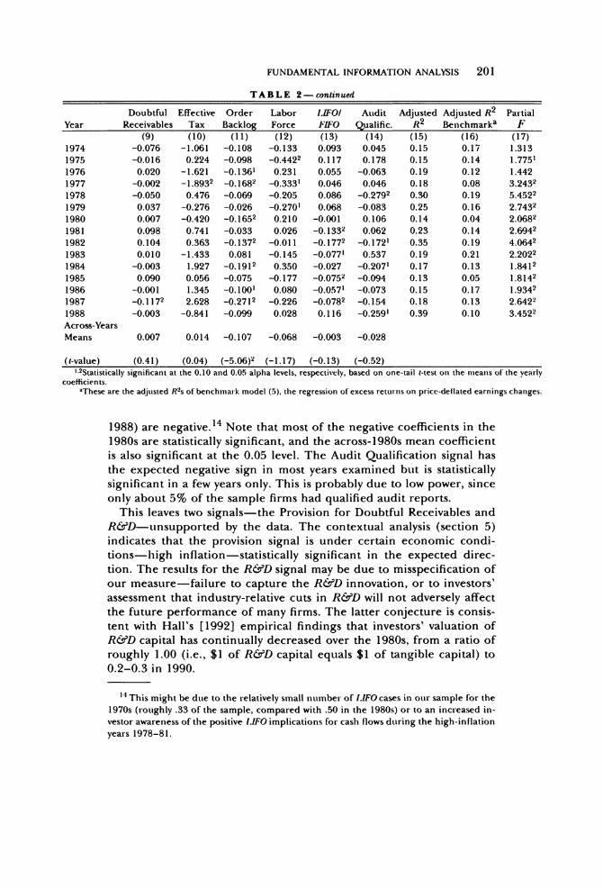
Doubtful Effective Order Labor LiFO/ Audit Adjusted Adjusted R2 Partial Year Receivables Tax Backlog Force FIFO Qualific. R2 Benchmarka F
(9) (10) (11) (12) (13) (14) (15) (16) (17) 1974 -0.076 -1.061 -0.108 -0.133 0.093 0.045 0.15 0.17 1.313 1975 -0.016 0.224 -0.098 -0.4422 0.117 0.178 0.15 0.14 1.7751 1976 0.020 -1.621 -0.1361 0.231 0.055 -0.063 0.19 0.12 1.442 1977 -0.002 -1.8932 -0.1682 -0.3331 0.046 0.046 0.18 0.08 3.2432 1978 -0.050 0.476 -0.069 -0.205 0.086 -0.2792 0.30 0.19 5.4522 1979 0.037 -0.276 -0.026 -0.2701 0.068 -0.083 0.25 0.16 2.7432 1980 0.007 -0.420 -0.1652 0.210 -0.001 0.106 0.14 0.04 2.0682 1981 0.098 0.741 -0.033 0.026 -0.1332 0.062 0.23 0.14 2.6942 1982 0.104 0.363 -0.1372 -0.011 -0.1772 -0.1721 0.35 0.19 4.0642 1983 0.010 -1.433 0.081 -0.145 -0.0771 0.537 0.19 0.21 2.2022 1984 -0.003 1.927 -0.1912 0.350 -0.027 -0.2071 0.17 0.13 1.8412 1985 0.090 0.056 -0.075 -0.177 -0.0752 -0.094 0.13 0.05 1.8142 1986 -0.001 1.345 -0.1001 0.080 -0.0571 -0.073 0.15 0.17 1.9342 1987 -0.1172 2.628 -0.2712 -0.226 -0.0782 -0.154 0.18 0.13 2.6422 1988 -0.003 -0.841 -0.099 0.028 0.116 -0.2591 0.39 0.10 3.4522 Across-Years Means 0.007 0.014 -0.107 -0.068 -0.003 -0.028
(t-value) (0.41) (0.04) (-5.06)2 (-1.17) (-0.13) (-0.52) l'2Statistically significant at the 0.10 and 0.05 alpha levels, respectively, based on one-tail t-test on the means of the year]
coefficients. 2These are the adjusted R2s of benchmark model (5), the regression of excess returns on price-deflated earnings change
1988) are negative.14 Note that most of the negative coefficients in the 1980s are statistically significant, and the across-1980s mean coefficient is also significant at the 0.05 level. The Audit Qualification signal has the expected negative sign in most years examined but is statistically significant in a few years only. This is probably due to low power, since only about 5% of the sample firms had qualified audit reports.
This leaves two signals-the Provision for Doubtful Receivables and R&D-unsupported by the data. The contextual analysis (section 5) indicates that the provision signal is under certain economic condi- tions-high inflation-statistically significant in the expected direc- tion. The results for the R&D signal may be due to misspecification of our measure-failure to capture the R&D innovation, or to investors' assessment that industry-relative cuts in R&D will not adversely affect the future performance of many firms. The latter conjecture is consis- tent with Hall's [1992] empirical findings that investors' valuation of R&D capital has continually decreased over the 1980s, from a ratio of roughly 1.00 (i.e., $1 of R&D capital equals $1 of tangible capital) to 0.2-0.3 in 1990.
14 This might be due to the relatively small number of LIFO cases in our sample for the 1970s (roughly .33 of the sample, compared with .50 in the 1980s) or to an increased in- vestor awareness of the positive LIFO implications for cash flows during the high-inflation years 1978-81.
202 BARUCH LEV AND S. RAMU THIAGARAJAN
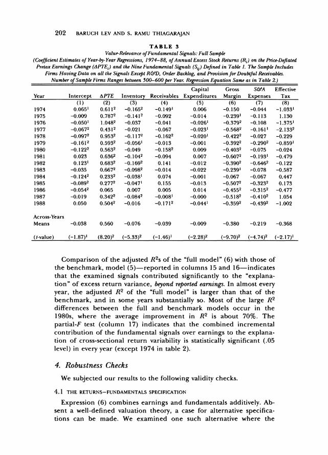
TABLE 3 Value-Relevance of Fundamental Signals: Full Sample
(Coefficient Estimates of Year-by-Year Regressions, 1974-88, of Annual Excess Stock Returns (Ri) on the Price-Deflated Pretax Earnings Change (APTED) and the Nine Fundamental Signals (Si.) Defined in Table 1. The Sample Includes
Firms Having Data on all the Signals Except R&D, Order Backlog, and Provision for Doubtful Receivables. Number of Sample Firms Ranges between 500-600 per Year. Regression Equation Same as in Table 2.)
Capital Gross S&A Effective Year Intercept APTE Inventory Receivables Expenditures Margin Expenses Tax
(1) (2) (3) (4) (5) (6) (7) (8) 1974 0.0651 0.6112 -0.1652 -0.1491 0.006 -0.150 -0.044 -1.033' 1975 -0.009 0.7872 -0.1412 -0.092 -0.014 -0.2391 -0.113 1.130 1976 -0.050' 1.0482 -0.037 -0.041 -0.0261 _0.3792 -0.108 -1.3751 1977 -0.0672 0.4312 -0.021 -0.067 -0.0231 -0.5682 -0.1611 -2.1332 1978 -0.0972 0.9532 -0.1172 -0.1622 -0.0201 -0.4222 -0.027 -0.229 1979 -0.1612 0.5932 -0.0561 -0.013 -0.001 -0.3922 -0.2902 -0.859' 1980 -0.1222 0.5632 -0.049 -0.1582 0.009 -0.4032 -0.075 -0.024 1981 0.023 0.6362 -0.1042 -0.094 0.007 -0.6072 -0.1931 -0.479 1982 0.1231 0.6832 -0.1692 0.141 -0.012 -0.3902 -0.6462 -0.122 1983 -0.035 0.6672 -0.0982 -0.014 -0.022 -0.2391 -0.078 -0.587 1984 -0.1242 0.2332 -0.0381 0.074 -0.001 -0.067 -0.067 0.447 1985 -0.0892 0.2772 -0.0471 0.155 -0.013 -0.5072 -0.3232 0.173 1986 -0.0542 0.065 0.007 0.005 0.014 -0.4552 -0.3152 -0.477 1987 -0.019 0.3422 -0.0842 -0.0081 -0.000 -0.5182 -0.4102 1.054 1988 0.050 0.5042 -0.016 -0.1712 -0.0441 -0.3592 -0.4392 -1.002
Across-Years Means -0.038 0.560 -0.076 -0.039 -0.009 -0.380 -0.219 -0.368
(t-value) (-1.87)1 (8.20)2 (-5.33)2 (-1.46)1 (-2.28)2 (-9.70)2 (-4.74)2 (-2.17)'
Comparison of the adjusted R2s of the "full model" (6) with those of the benchmark, model (5)-reported in columns 15 and 16-indicates that the examined signals contributed significantly to the "explana- tion" of excess return variance, beyond reported earnings. In almost every year, the adjusted R2 of the "full model" is larger than that of the benchmark, and in some years substantially so. Most of the large R2 differences between the full and benchmark models occur in the 1980s, where the average improvement in R2 is about 70%. The partial-F test (column 17) indicates that the combined incremental contribution of the fundamental signals over earnings to the explana- tion of cross-sectional return variability is statistically significant (.05 level) in every year (except 1974 in table 2).
4. Robustness Checks
We subjected our results to the following validity checks.
4.1 THE RETURNS-FUNDAMENTALS SPECIFICATION
Expression (6) combines earnings and fundamentals additively. Ab- sent a well-defined valuation theory, a case for alternative specifica- tions can be made. We examined one such alternative where the
FUNDAMENTAL INFORMATION ANALYSIS 203
T A B L E 3-continued
Labor LIFOI Audit Adjusted Adjusted R2 Partial Year Force FIFO Qualifications R2 Benchmarka F
(9) (10) (11) (12) (13) (14) 1974 -0.2612 0.062 0.029 0.15 0.17 3.5192 1975 -0.146 0.037 -0.001 0.15 0.14 2.0712 1976 -0.000 0.060 -0.060 0.19 0.12 3.0752 1977 -0.114 0.101 -0.036 0.18 0.08 7.0672 1978 -0.1892 0.039 -0.012 0.30 0.19 5.0272 1979 -0.1852 -0.008 -0.037 0.25 0.16 3.7322 1980 0.186 -0.0992 0.048 0.14 0.04 6.0962 1981 0.007 -0.0381 -0.010 0.23 0.14 3.5932 1982 -0.0772 -0.1322 -0.1882 0.35 0.19 10.1392 1983 -0.3042 -0.006 0.134 0.19 0.21 2.8922 1984 0.087 -0.0482 -0.1492 0.17 0.13 2.1412 1985 -0.1512 -0.0381 -0.1772 0.13 0.05 6.2982 1986 0.020 -0.0562 0.103 0.15 0.17 4.3582 1987 -0.011 -0.026 0.042 0.18 0.13 5.7342 1988 0.018 0.084 -0.057 0.39 0.10 2.6492
Across-Years Means -0.075 -0.005 -0.025
(t-value) (-2.15)2 (-0.26) (-1.02)
",2Statistically significant at the 0.10 and 0.05 alpha levels, respectively, based on one-tail t-test on the means of the yearly coefficients.
aThese are the adjusted R2 of benchmark model (5), the regression of excess returns on price- deflated earnings changes.
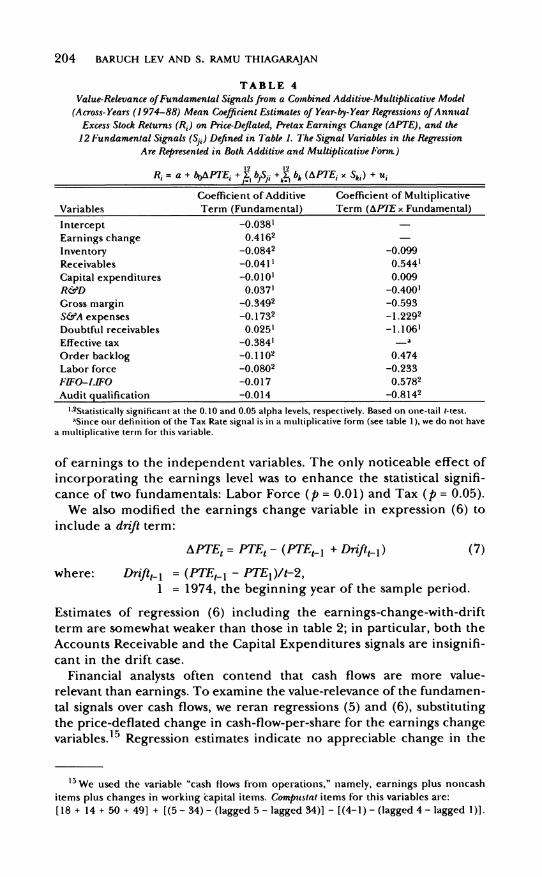
message of the fundamentals is assumed to depend on the size of the earnings surprise. Specifically, regression (6) is modified to include 12 fundamentals and earnings change interaction terms:
12 12
Ri = a + boAPTEi + X b-S.- + X- bk(APTEi x Ski) + uv. (6a)
Across-years mean coefficient estimates of expression (6a) are reported in table 4. All the fundamentals that were statistically significant in ta- ble 2 are also significant in table 4. The multiplicative term of the Au-
dit Qualification signal is statistically significant here while its additive
counterpart was not in table 2. The multiplicative R&D and Doubtful
Receivables variables have the expected sign and are significant, yet their additive counterparts (left column) have the "wrong" sign and are
also significant. We cannot explain this finding. The multiplicative
specification (6a) thus supports the additive one; given that expression (6) is more parsimonious, we decided to use it in the following contex- tual analysis reported in section 5.
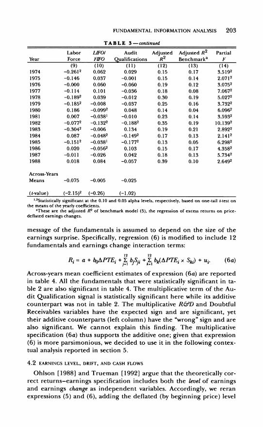
4.2 EARNINGS LEVEL, DRIFT, AND CASH FLOWS
Ohlson [1988] and Trueman [1992] argue that the theoretically cor-
rect returns-earnings specification includes both the level of earnings and earnings change as independent variables. Accordingly, we reran
expressions (5) and (6), adding the deflated (by beginning price) level
204 BARUCH LEV AND S. RAMU THIAGARAJAN
TABLE 4 Value-Relevance of Fundamental Signals from a Combined Additive-Multiplicative Model
(Across-Years (1974-88) Mean Coefficient Estimates of Year-by-Year Regressions of Awnntal
Excess Stock Returns (Ri) on Price-Deflated, Pretax Earnings Change (APTE), and the
12 Fundamental Signals (Sji) Defined in Table 1. The Signal Variables in the Regression Are Represented in Both Additive and Multiplicative Form.)
12 1 2 R= a + b0APTE, + L] b-S.- + X
bk (APTEj x Ski) + u.
Coefficient of Additive Coefficient of Multiplicative
Variables Term (Fundamental) Term (APTE x Fundamental)
Intercept -0.0381
Earnings change 0.4162 Inventory -0.0842 -0.099
Receivables -0.0411 0.544'
Capital expenditures -0.010' 0.009
R&D 0.0371 -0.4001
Gross margin 0.3492 -0.593
S&A expenses -0.1732 -1.2292 Doubtful receivables 0.0251 -1.1061
Effective tax -0.3841 a
Order backlog -0.11 02 0.474 Labor force -0.0802 -0.233
FIFO-LIFO -0.017 0.5782
Audit qualification -0.014 -0.8142
l"2Statistically significant at the 0.10 and 0.05 alpha levels, respectively. Based on one-tail t-test. aSince our definition of the Tax Rate signal is in a multiplicative form (see table 1), we do not have
a multiplicative term for this variable.
of earnings to the independent variables. The only noticeable effect of incorporating the earnings level was to enhance the statistical signifi- cance of two fundamentals: Labor Force (p = 0.01) and Tax (p = 0.05).
We also modified the earnings change variable in expression (6) to include a drift term:
APTEt = PTEt - (PTE1-I + Driftt- 1) (7)
where: DrifttI = (PTEt- - PTE1)/t-2, 1 = 1974, the beginning year of the sample period.
Estimates of regression (6) including the earnings-change-with-drift term are somewhat weaker than those in table 2; in particular, both the Accounts Receivable and the Capital Expenditures signals are insignifi- cant in the drift case.
Financial analysts often contend that cash flows are more value- relevant than earnings. To examine the value-relevance of the fundamen- tal signals over cash flows, we reran regressions (5) and (6), substituting the price-deflated change in cash-flow-per-share for the earnings change variables.15 Regression estimates indicate no appreciable change in the
15 We used the variable "cash flows from operations," namely, earnings plus noncash
items plus changes in working capital items. Compustat items for this variables are:
[18 + 14 + 50 + 49] + [(5- 34)- (lagged 5 - lagged 34)] - [(4-1) - (lagged 4- lagged 1)].
FUNDAMENTAL INFORMATION ANALYSIS 205
statistical significance of the fundamentals or in their contribution to R2 when cash flows are substituted for earnings.
4.3 RAW RETURNS
The regression analysis described above was replicated with raw re- turns substituting for excess returns. Overall, the value-relevance of the fundamental signals with respect to raw returns appears somewhat stronger than that for excess returns. For example, the average R2 of the full model (6) over the 1980s, 0.17, is 140% higher than the "earn- ings alone" R2, 0.07. With respect to the individual fundamentals, the R&D and the Audit Qualification signals are statistically significant at the 0.05 level (across all years), whereas they were insignificant with re- spect to excess returns (table 2).
4.4 SIZE EFFECTS
To examine whether the fundamentals proxy for firm size, we reran regression (6) adding a size variable-market value of equity (total capitalization) at year-end. While the firm size coefficient was statisti- cally significant (0.08 level across years), none of the findings and con- clusions reported above was affected.
4.5 ECONOMETRIC DIAGNOSTICS
Examination of the correlation matrix (Pearson and Spearman) for all the variables considered in this study reveals only four relatively large correlation coefficients. The change in earnings before tax is cor- related with its components, Gross Margin (-0.35) and S&A Expenses (-0.24). The negative signs of these correlations result from the defini- tion of the latter two signals as sales minus gross margin or S&A ex- penses. The other relatively large correlations are Gross Margin and S&A Expenses (-0.21), and Receivables with the Provision for Doubtful Receivables (0.35). Overall, then, multicollinearity does not seem to pose a serious problem in our analysis. White's [1980] heteroscedastic- ity test indicated that homoscedasticity cannot be rejected at conven- tional levels (alpha level of 0.05) for any year analyzed.
5. Conditioning the Analysis on Macroeconomic Variables
Previous research on the value-relevance of earnings and other fun- damentals was generally conducted in an unconditioned (noncontex- tual) mode. 16 We now extend the preceding analysis to allow for different economic conditions, the importance of which is demon- strated by the following example.
Following analysts, we conjectured above that a disproportionate (to sales) increase in receivables conveys bad news. Yet, for a given receivables
16Wilson [1986] and Bernard and Stober [1989], on the value-relevance of cash flows vs. earnings, are among the few exceptions.
206 BARUCH LEV AND S. RAMU THIAGARAJAN
increase, the negative message is likely to be more pronounced as the rate of inflation increases. The reason is that since receivables' carrying costs increase with inflation, firms are expected to respond by decreasing the receivables level. Given an expectation of reduced receivables during in- flation, an observed disproportionate increase of this item naturally con- veys a stronger negative signal than an identical receivables change during a low-inflation period.
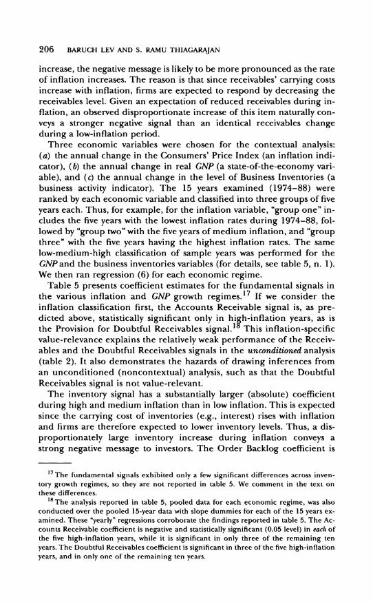
Three economic variables were chosen for the contextual analysis: (a) the annual change in the Consumers' Price Index (an inflation indi- cator), (b) the annual change in real GNP (a state-of-the-economy vari- able), and (c) the annual change in the level of Business Inventories (a business activity indicator). The 15 years examined (1974-88) were ranked by each economic variable and classified into three groups of five years each. Thus, for example, for the inflation variable, "group one" in- cludes the five years with the lowest inflation rates during 1974-88, fol- lowed by "group two" with the five years of medium inflation, and "group three" with the five years having the highest inflation rates. The same low-medium-high classification of sample years was performed for the GNP and the business inventories variables (for details, see table 5, n. 1). We then ran regression (6) for each economic regime.
Table 5 presents coefficient estimates for the fundamental signals in the various inflation and GNP growth regimes.17 If we consider the inflation classification first, the Accounts Receivable signal is, as pre- dicted above, statistically significant only in hi'h-inflation years, as is the Provision for Doubtful Receivables signal.' This inflation-specific value-relevance explains the relatively weak performance of the Receiv- ables and the Doubtful Receivables signals in the unconditioned analysis (table 2). It also demonstrates the hazards of drawing inferences from an unconditioned (noncontextual) analysis, such as that the Doubtful Receivables signal is not value-relevant.
The inventory signal has a substantially larger (absolute) coefficient during high and medium inflation than in low inflation. This is expected since the carrying cost of inventories (e.g., interest) rises with inflation and firms are therefore expected to lower inventory levels. Thus, a dis- proportionately large inventory increase during inflation conveys a strong negative message to investors. The Order Backlog coefficient is
17 The fundamental signals exhibited only a few significant differences across inven- toi-y growth regimes, so they are not reported in table 5. We comment in the text on these differences.
18 The analysis reported in table 5, pooled data for each economic regime, was also conducted over the pooled 15-year data with slope dummies for each of the 15 years ex- amined. These "yearly" regressions corroborate the findings reported in table 5. The Ac- counts Receivable coefficient is negative and statistically significant (0.05 level) in each of the five high-inflation years, while it is significant in only three of the remaining ten years. The Doubtful Receivables coefficient is significant in three of the five high-inflation years, and in only one of the remaining ten years.
FUNDAMENTAL INFORMATION ANALYSIS 207
TABLE 5 Value-Relevance of Fundamental Signals Conditioned o t Macroeconomic Variables
(Coefficient Estimates from Regressions of Excess Stock Returns (Ri) on Price-Deflated Pretax Earnings Change (APTE), and the 12 Fundamental Signals (Sji) Defined in Table 1. For Each Economic Variable-Inflation, GNP Growth, and Business Inventories-the Fifteen Years Examined, 1974-88, Were Ranked and Classified into Three Groups of Five Years
Each: High Values of the Variable, Median, and Low Values. The Regressions Were Run on the Pooled, Five- Year Data of Each Group. The Estimates for Business Inventories Are Not
Presented in the Table, but Are Commented on in the Text.)
12 Ri= a + b0APTEi + Z bjSji + vi
Inflation Ratea GNP Growtha Independent Variable High Medium Low High Medium Low
Intercept -0.0262 -0.0682 -0.0382 -0.0802 -0.0702 0.0302 APTE 0.6412 0.6232 0.3222 0.5872 0.3352 0.6842 Inventory -0.0672 -0.0892 -0.0362 -0.0532 -0.0622 -0.0982 Receivables -0.1422 -0.016 0.012 -0.0552 0.017 -0.0602 Capital expenditures 0.007 -0.009' -0.008 -0,0122 -0.002 0.006 R&D -0.028 0.020 0.032 -0.019 -0.006 0.029 Gross margin -0.3062 -0.3072 -0.4582 -0.2972 _0.4792 -0.3692 S&A expenses -0.2322 -0.027 -0.3612 -0.028 -0.2742 -0.2992 Doubtful receivables -0.042' 0.034 0.019 -0.006 0.024 -0.016 Effective tax _0.4592 -0.6142 -0.240 -0.7822 _0.7372 -0.298 Order backlog -0.0812 -0.1092 -0.1502 -0.1162 -0.1122 -0.1242 Labor force -0.008 -0.1302 -0.0772 -0.0772 -0.1092 -0.004 FIFO-LIFO -0.006 0.0212 -0.2102 0.052 -0.0312 -0.0272 Audit qualification 0.018 -0.0452 0.050 -0.035' 0.013 0.001
1,Statistically significant at the 0.10 and 0.05 alpha levels, respectively. Based on one-tail t-test. aThe classification of years examined, 1974-88, into groups of High, Medium, and Low inflation
rates and GNPgrowth is shown below. Annual percentage changes in parentheses.
Low Medium High Inflation 1983(3.2), 1985(3.6), 1976(5.8), 1977(6.5), 1974(11.0), 1975(9.1),
1986(1.9), 1987(3.6), 1978(7.6), 1982(6.2), 1979(11.3), 1980(13.5), 1988(4.1). 1984(4.3). 1981(10.3).
GNP 1974(-0.5), 1975(-1.3), 1979(2.5), 1983(3.6), 1976(4.9), 1977(4.7), Growth 1980(-0.2), 1981(1.9), 1985(3.4), 1986(2.7), 1978(5.3), 1984(6.8),
1982(-2.5). 1987(3.7). 1988(4.4). The values of the economic variables were obtained from the Economic Report of the President (Washing- ton, D.C.: United States Government Printing Office, January 1992).
increasing (absolute) with the decrease in inflation rate; the difference between the coefficients in the high- and low-inflation environments (-0.081 and -0.150) is statistically significant at the 0.05 level. This is ex- pected; during high inflation, a given increase in the dollar value order backlog will reflect, among other things, a large inflationary component and therefore relatively low real sales growth relative to a similar backlog increase reported during low-inflation years. The latter, therefore, sends a stronger signal about future real performance to investors.
Regarding GNP growth regimes, the data in table 5 indicate that the coefficient of the inventory signal is lowest (absolute) in the high- growth years (the difference between the high- and low-growth inventory
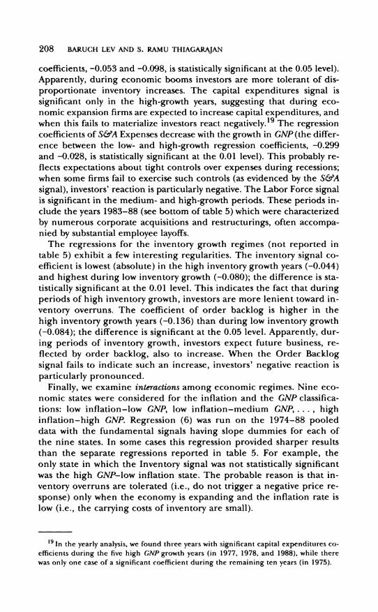
208 BARUCH LEV AND S. RAMU THIAGARAJAN
coefficients, -0.053 and -0.098, is statistically significant at the 0.05 level). Apparently, during economic booms investors are more tolerant of dis- proportionate inventory increases. The capital expenditures signal is significant only in the high-growth years, suggesting that during eco- nomic expansion firms are expected to increase capital expenditures, and when this fails to materialize investors react negatively.'9 The regression coefficients of S&A Expenses decrease with the growth in GNP (the differ- ence between the low- and high-growth regression coefficients, -0.299 and -0.028, is statistically significant at the 0.01 level). This probably re- flects expectations about tight controls over expenses during recessions; when some firms fail to exercise such controls (as evidenced by the S&A signal), investors' reaction is particularly negative. The Labor Force signal is significant in the medium- and high-growth periods. These periods in- clude the years 1983-88 (see bottom of table 5) which were characterized by numerous corporate acquisitions and restructurings, often accompa- nied by substantial employee layoffs.
The regressions for the inventory growth regimes (not reported in table 5) exhibit a few interesting regularities. The inventory signal co- efficient is lowest (absolute) in the high inventory growth years (-0.044) and highest during low inventory growth (-0.080); the difference is sta- tistically significant at the 0.01 level. This indicates the fact that during periods of high inventory growth, investors are more lenient toward in- ventory overruns. The coefficient of order backlog is higher in the high inventory growth years (-0.136) than during low inventory growth (-0.084); the difference is significant at the 0.05 level. Apparently, dur- ing periods of inventory growth, investors expect future business, re- flected by order backlog, also to increase. When the Order Backlog signal fails to indicate such an increase, investors' negative reaction is particularly pronounced.
Finally, we examine interactions among economic regimes. Nine eco- nomic states were considered for the inflation and the GNP classifica- tions: low inflation-low GNP, low inflation-medium GNP,., high inflation-high GNP. Regression (6) was run on the 1974-88 pooled data with the fundamental signals having slope dummies for each of the nine states. In some cases this regression provided sharper results than the separate regressions reported in table 5. For example, the only state in which the Inventory signal was not statistically significant was the high GNP-low inflation state. The probable reason is that in- ventory overruns are tolerated (i.e., do not trigger a negative price re- sponse) only when the economy is expanding and the inflation rate is low (i.e., the carrying costs of inventory are small).
19 In the yearly analysis, we found three years with significant capital expenditures co- efficients during the five high GNP growth years (in 1977, 1978, and 1988), while there
was only one case of a significant coefficient during the remaining ten years (in 1975).
FUNDAMENTAL INFORMATION ANLYSIS 209
The high GNP-low inflation state also yields the largest and most significant Capital Expenditures coefficient. Apparently, when the economy is booming and the cost of capital is low, investors penalize firms that fail to keep up their capital expenditures with other firms in the industry. Medium GNP-high inflation is the only state where the R&D signal is significant. The Doubtful Receivables coefficient is larg- est and most statistically significant for the low GNP-high inflation state, probably because recession and high inflation lead to bankrupt- cies and loan defaults, so firms are expected to increase their doubtful receivables' provisions.
6. Linking Research Strands: Fundamientals-Persistence- Response Coefficient
The persistence of earnings has received considerable attention (e.g., Kormendi and Lipe [1987], Easton and Zmijewski [1989], Collins and Kothari [1989], and Thiagarajan [1989]). The main objective of the persistence research is to gain insight into differential investor reaction to earnings announcements. Indeed, estimates of earnings persistence, often derived from the time series of earnings or from revisions of analysts forecasts around earnings announcements, were found to be correlated with the size of the earnings response co- efficient. Still unexplored, however, is the question of how investors operationally determine earnings persistence. It seems unlikely, for example, that they use ARIMA models for this purpose.
Our search of analysts' sources revealed repeated references to "qual- ity of earnings," which seems to reflect in ,eneral analysts' perceptions of the degree of earnings persistence.' For example, Value Line [1973a] proposed to adjust reported earning to "quality earnings" by removing one-time (transitory) items and accounting for questionable items, such as interest capitalization. Our discussion in section 2 indi- cates that analysts use fundamentals to draw explicit inferences about the persistence of earnings. Thus, for example, an earnings increase ac- companied by an order backlog buildup enhances confidence in the continuation of the earnings improvement, while an earnings increase brought about by a one-time effective tax rate decrease is unlikely to persist. Thus, a major use of the fundamentals is to allow investors to as- sess earnings persistence and growth.21 The following tests are aimed at
20 0n quality of earnings, see, for example, Bernstein and Siegel [1979], Siegel [1982], Comiskey [1982], Fabozzi [1978], Imhoff [1989], and Imhoff and Thomas [1989].
21 There is, of course, a distinction between earnings persistence-the continuation of earnings at the current level-and growth. It is doubtful, however, whether at this stage we could clearly discriminate between fundamentals indicating persistence and those suggesting growth. The message in the fundamentals appears to reflect a combina- tion of both patterns.
210 BARUCH LEV AND S. RAMU THIAGARAJAN
examining this conjecture, thereby linking our fundamental analysis to the earnings persistence and response coefficient literature.
6.1 FUNDAMENTAL SIGNALS AND THE RESPONSE COEFFICIENT
If the fundamental signals help to assess earnings persistence, then an aggregate "fundamental score," reflecting the combined message in the signals, should be associated with the earnings response co- efficient: firms characterized by "high-quality" fundamental scores should exhibit large response coefficients relative to firms with "low- quality" scores. Accordingly, we constructed an aggregate fundamental score for each sample firm and year as follows: each of the fundamental signals listed in table 1 was computed for every firm and assigned a value of 1 for a positive signal and 0 for a negative signal. These num- bers were then summed for each firm and year and standardized by the number of available fundamentals, to yield an aggregate fundamental score.22 Recall that a positive value for a signal (e.g., an inventory growth larger than sales) implies "bad news," and vice versa for a nega- tive number. Thus, low fundamental scores (O at the limit) indicate high quality of earnings (persistence), while large fundamental scores imply low quality.
We divided the sample firms for each year into five groups, based on their aggregate fundamental scores. We then ran for each year the conventional, cross-sectional returns-earnings regression (expression 5) with slope dummies for each of the five score groups, to estimate the earnings response coefficient for each score (earnings quality) group. Table 6 presents the yearly earnings response coefficients for each score group, in descending order of earnings quality (i.e., in an in- creasing order of the aggregate score). For 12 of the 15 years examined the highest-quality (group 1) response coefficient is larger than the lowest-quality (group 5) response coefficient, and in 10 of the 12 years the difference is statistically significant (see t-values). Even more strik- ing, in each of the 15 years examined, the response coefficient of the firms in group 5-the lowest-quality scores-is lower than the co- efficients of either quality group 1 or 2.
The tendency of the earnings response coefficients in table 6 to de- crease from the highest earnings quality group to the lowest is not strictly monotonic. This is probably due to the rather coarse nature of the aggregate fundamental score, in particular to the fact that the indi- vidual fundamental signals constituting the score are equally weighted. Thus, for example, the highly value-relevant order backlog signal (table 2) is equally weighted in the total score with the less value- relevant accounts receivables signal. Nevertheless, a clear association
22A1I the conclusions drawn on the basis of the dummy-based score hold for a para- metric aggregate score, based on the actual values of the signals, rather than on a 0, 1 dummy.
FUNDAMENTAL INFORMATION ANALYSIS 211
TABLE 6 Fundamental Signals and Earnings Response Coefficients
(Estimated Coefficients of Price-Deflated Annual Earnings Changes, from Regressions of Annual Excess Returns (Ri) on Earnings Changes (AEj). Regressions Were Run for Each Sample Year (1974-88), with
Slope Dummies (Response Coefficients) for Each of Five Groups of Firms Classified by the Aggregate Fundamental Score (ASj). The Aggregate Fundamental Score Combines the 12 Signals Defined in
Table I and Reflects the Quality-Persistence of Earnings.a)
R. = a + bjAEjAS1 + * +b5AEiAS5- + ui
Fundamental Score Group 1974 1975 1976 1977 1978 1979 1980 1981
1 (highest quality) 1.181 1.179 1.212 1.737 1.162 0.980 0.695 1.543 2 2.015 0.478 0.787 2.392 1.301 1.393 2.265 1.027 3 0.995 0.318 1.161 1.132 1.451 0.520 1.051 1.267 4 0.982 0.968 1.136 2.210 1.441 0.845 0.962 0.761 5 (lowest quality) 1.545 0.288 0.545 0.621 0.992 0.557 0.408 0.972
t-value of "high" minus "low" -1.40 4.822 3.202 3.842 0.87 2.211 1.661 2.612
Fundamental Score Group 1982 1983 1984 1985 1986 1987 1988 1 (highest quality) 1.513 0.757 0.436 0.559 0.495 0.623 1.944 2 0.863 1.354 1.237 0.696 0.315 1.094 2.528 3 0.807 1.056 0.658 0.805 0.782 0.773 1.669 4 1.251 0.396 0.400 1.145 0.448 0.955 0.264 5 (lowest quality) 0.442 0.324 0.848 0.500 0.109 0.653 0.578
t-value of "high" minus "low" 5.602 2.021 -2.01 0.40 2.822 -0.19 4.132
l 2Statistically significant at the 0.05 and 0.01 alpha levels, respectively. aTotal number of observations in the yearly regressions ranges between 681 and 1,495.
exists between the message conveyed by the fundamentals and the earnings response coefficient, indicating that the fundamentals are used by investors to assess the persistence of earnings.
Given that earnings persistence is sometimes estimated from the time series of earnings, we wished to compare the ability of the fundamentals to indicate persistence with that of time-series measures. Accordingly, the Kormendi and Lipe [1987] time-series persistence measure was computed for each sample firm over the period 1970-88. The aggre- gate fundamental score is, however, year-specific, so we chose the me- dian yearly score to represent the fundamentals during the 1970-88 period for each sample firm. We then ranked the sample firms first by their median fundamental score, reflecting the quality of earnings, and then by their time-series persistence measure, and formed four groups of firms: High Quality-High Time-Series persistence (HQ-HT), High
23 "High" refers to the top 20% of the firms in the quality persistence dimension and "low" refers to the bottom 20%. The choice of the top/bottom 20% to represent high/low quality was made to improve the power of the tests. The analysis was repeated by redefin- ing high/low as the top/bottom third with no change in results.
212 BARUCH LEV AND S. RAMU THIAGARAJAN
Quality-Low Time-Series (HQ-LT), Low Quality-High Time-Series (LQ-HT), and Low Quality-Low Time-Series (LQ-LT). The returns- earnings regression (5) was then run for each of these four groups (pooling the data over 1974-88), yielding four earnings response co- efficients presented in table 7.
The differences between the earnings response coefficients of the high- and low-quality (fundamental scores) groups (3.241 vs. 0.662 and 2.663 vs. 0.492) are large and statistically significant (at the 0.01 level), whereas the differences along the high-low time-series persistence dimension (3.241 vs. 2.663 and 0.662 vs. 0.492) are much smaller and statistically insignificant (at the 0.05 level). This suggests that the fun- damental signals, as reflected by the quality scores, capture more fully investors' assessment of the persistence of earnings (indicated by the response coefficient) than does the time-series persistence measure. Furthermore, the fundamental signals can be estimated on a timely basis-quarterly or annually-rather than from a long and sometimes unstable time series of earnings.
6.2 FUNDAMENTAL SIGNALS AND FUTURE EARNINGS
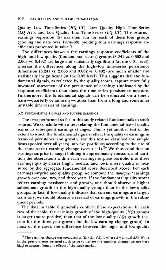
The tests performed so far in this study related fundamentals to stock returns. We conclude with a test relating the fundamental-based quality scores to subsequent earnings changes. This is yet another test of the extent to which the fundamental signals reflect the quality of earnings in terms of persistence and growth. For this test we classified the sample firms (pooled over all years) into five portfolios according to the size of the most recent earnings change (year t - 1).24 We thus condition on earnings surprise (change) holding it approximately constant, and parti- tion the observations within each earnings surprise portfolio into three earnings quality classes (high, median, and low), where quality is mea- sured by the aggregate fundamental score described above. For each earnings surprise and quality group, we compute the subsequent earnings growth over one, two, and three years. If the fundamental quality scores reflect earnings persistence and growth, one should observe a higher subsequent growth in the high-quality groups than in the low-quality groups. In fact, if low quality indicates that current earnings are largely transitory, we should observe a reversal of earnings growth in the subse- quent periods.
The data in table 8 generally confirm these expectations. In each row of the table, the earnings growth of the high-quality (HQ) groups is larger (more positive) than that of the low-quality (LQ) growth (ex- cept for the three-year growth for the low earning change group). In most of the cases, the difference between the high- and low-quality
24 The earnings change was measured as (Et - Et 1)IjE1 1j, where E = annual EPS. While in the previous tests we used stock price to deflate the earnings change, we use here
1E111 to abstract from any effects of the stock market.
FUNDAMENTAL INFORMATION ANALxYSIS 213
TABLE 7 Response Coefficients forFirms Classified by Fundamental Scores and Time-Series Persistence Measures
(The Pooled Sample Firms (1974-88) Were First Ranked on a Time-Series Measure of Earnings Persistence and Then Ranked on Their Aggregate Fundamental Quality Score Measure. The
Firms Were Then Classified into Four Groups According to High-Low Time-Series Persistence and Quality Score Measures (High and Low Refers to Top/Bottom 20 % of the Ranking). The
Numbers in the Table Are the Earnings Response Coefficients from Regressing Excess Stock Returns on Annual Earnings Changes for Firms within Each of the Four Groups.)
Fundamental Earnings Quality High Low
High 3.241 0.662 Time-Series (3.63)a (7.48) Persistence
Low 2.663 0.492
(4.63) (4.39) at-valiues.
TABLE 8 Fundamental Signals and Subsequent Earnings Changes
(Sample Firms, Pooled over Years (1974-88), Were Classified into Five Groups according to the Size of Current Year's Earnings Change (Relative to Last Yea?). Within Each of These Five Groups,
the Firms Were Classified into Three Earnings Quality Groups according to the Firms' Aggregate Fundamental Score: High, Medium, and Low Quality. The Numbers in the
Table Are the Average One- to Three- Year-Ahead Earnings Changes for Each Group of Current Earnings Change and Earnings Quality.)
Subsequent Earnings Changesa
Current Year's Earnings One Year Ahead Two Years Ahead Three Years Ahead
Change HQb MQb LQb HQ MQ LQ HQ MQ LQ
Low 2.08 1.33 1.86 -0.802 -1.11 -1.77 -0.61 -0.76 -0.36 Medium 1 0.202 -0.37 -0.46 0.122 -0.43 -0.56 0.042 -0.30 -0.49 Medium 2 -0.032 -0.04 -0.26 0.10' 0.10 -0.10 0.17 0.12 0.08 Medium 3 0.122 -0.09 -0.38 0.362 0.18 -0.03 0.482 0.29 0.21 High 0.07 -0.16 -0.26 2.78 2.02 2.43 1.63 1.76 1.06 All cases 0.492 0.13 0.10 0.51' 0.15 -0.01 0.34 0.22 0.10
I"2The difference between the HQ and the LQgrowth rates is statistically significant at the 0.05 and 0.01 alpha levels, respectively.
aThe earnings change is defined as the change in subsequent earnings divided by the absolute value of the prior period's earnings, see n. 24 in the text.
bHQ, MQ, and LQ are high, medium, and low quality of earnings, respectively, measured by the aggregate fundamental score obtained from aggregating for each firm the signals defined in table 1. HQ, MQ, and LQ include one-third each of the sample firms.
growth rates is statistically significant, at the .05 level or better. For ex- ample, for "all cases" (bottom line of table 8), the one-year growth rate of firms with high-quality scores, 0.49, is significantly larger than the growth rate of the low-quality firms, 0.10.25 Also as expected, the earn- ings changes of the low-quality (transitory earnings) groups are in most
25 The grouping of firms in table 8 into five classes of earnings change and three qual- ity classes is, of course, arbitrary. Experimentation with several alternative number of classes yielded results similar to those in the table.
214 BARUCH LEV AND S. RAMU THIAGARAJAN
cases negative (earnings reversals), indicating that the fundamental score captures the transitory component of earnings. The fundamental signals are thus associated in the expected direction with future earn- ings changes, and as such reflect the persistence of earnings.
7. Concluding Remarks
This study is aimed at extending and linking several lines of investi- gation in capital markets accounting research. In particular, we focus on the areas of value-relevant fundamentals, contextual (conditioned) returns-fundamentals analysis, and the relation among fundamentals, earnings persistence, and the earnings response coefficient. Our iden- tification of value-relevant fundamentals in this study differs from pre- vious attempts in that it was guided by analysts' descriptions rather than by a statistical search procedure. This study also differs from oth- ers in conditioning the fundamentals on macrovariables. As expected, such a contextual analysis provides several insights which go unnoticed in an unconditioned analysis. Essentially, we find most of the examined fundamentals to be value-relevant during the period 1974-88.
The fundamentals identified as value-relevant in the first stage of the study were used to link the research on nonearnings information with that on the persistence of earnings and the response coefficient. This was done by hypothesizing that investors use the fundamentals to assess the extent of earnings persistence and growth. We validated this hy- pothesis by demonstrating a statistically significant relation between an aggregate fundamental score, indicating the quality of earnings, and the earnings response coefficient. The hypothesis was further corrobo- rated by demonstrating a relation between firms' fundamental scores and subsequent earnings growth.
REFERENCES
BERNARD, V. "Cross-Sectional Dependence and Problems in Inference in Market-Based Accounting Research." Journal of Accounting Research (Spring 1987): 1-48.
BERNARD, V., AND T. STOBER. "The Nature and Amount of Information in Cash Flows and Accruals." The Accounting Review (October 1989): 624-52.
BERNSTEIN, L. Financial Statement Analysis. Homewood, Ill.: Irwin, 1988. BERNSTEIN, L., AND J. SIEGEL. "The Concept of Earnings Quality." Financial Analysts Journal
(July/August 1979): 72-75. BLINDER, A., AND L. MACCINI. "Taking Stock: A Critical Assessment of Recent Research on
Inventories." Journal of Economic Perspectives (Winter 1991): 73-96. CARROLL, T.; D. COLLINS; AND B. JOHNSON. "The LIFO-FIFO Choice and the Quality of
Earnings Signal." Working paper, University of Iowa, 1991. COLLINS, W., AND S. KOTHARI. "An Analysis of Intertemporal and Cross-Sectional Determi-
nants of Earnings Response Coefficients." Journal of Accounting and Economics (July 1989): 143-82.
CoMIsKFY, E. "Assessing Financial Quality: An Organizing Theme for Credit Analysis." Journal of Commercial Bank Lending (December 1982): 32- 47.
EASTON, P., AND M. ZMIJEWSKI. "Cross-Sectional Variation in the Stock Market Response to Accounting Earnings Announcements." Journal of Accounting and Economics (July 1989): 117-41.

FUNDAMENTAL INFORMATION ANALYSIS 215
FABOZZI, F. "Quality of Earnings: A Test of Market Efficiency.' Journal of Portfolio Manage- ment (Fall 1978): 53-56.
FAZZARI, S.; G. HUBBARD; AND B. PETERSON. "Financing Constraints and Corporate Invest- ment." Brookings Papers on Economic Activity 1 (1988): 141-206.
GRABOWSKI, H. "Industrial Research and Development, Intangible Capital Stocks, and Firm Profit Rates." Bell Journal of Economics (Autumn 1978): 328- 43.
GRAHAM, B.; D. DODD; S. COTTLE; AND C. TATHAM. Security Analysis. New York: McGraw-Hill, 1962.
HALL, B. "The Value of Intangible Corporate Assets: An Empirical Study of the Compo- nents of Tobin's Q." Working paper, University of California, Berkeley, and the Na- tional Bureau of Economic Research, December 1992.
HAWKINS, D. Corporate Financial Reporting and Analysis. Homewood, Ill.: Dow Jones-Irwin, 1986.
HOLTHAUSEN, R., AND D. LARCKER. "The Prediction of Stock Returns Using Financial State- ment Information." Journal of Accounting and Economics (July/September 1992): 373-411.
IMHOFF, E. "Accounting Quality: Economic Content." Working paper, University of Mich- igan, 1989.
IMHOFF, E., AND J. THOMAS. "Accounting Quality." Working paper, University of Michigan, 1989.
KORMENDI, R., AND R. LIPE. "Earnings Innovations, Earnings Persistence, and Stock Re- turns." Journal of Business (July 1987): 323-45.
McNiCHOLS, M., AND P. WILSON. "Evidence of Earnings Management from the Provision for Bad Debts." Journal of Accounting Research (Supplement 1988): 1-31.
O'GLOVE, T. Quality of Earnings. New York: The Free Press, 1987. OHLSON, J. "Accounting Earnings, Book Value, and Dividends: The Theory of the Clean
Surplus Equation." Working paper, Columbia University, 1988. OMER, K.; K. MOLLOY; AND D. ZIEBART. "Measurement of Effective Corporate Tax Rates Using
Financial Information." Journal of American Taxation Association (Spring 1991): 57-72. OU, J., AND S. PENMAN. "Financial Statement Analysis and the Prediction of Stock Re-
turns." Journal of Accounting and Economics (November 1989): 295-329. PORCANO, T. "Corporate Tax Rates: Progressive, Proportional or Regressive." Journal of
American Taxation (Spring 1986): 17-31. SIEGEL, J. "The 'Quality of Earnings' Concept-A Survey." Financial Analysts Journal
(March/April 1982): 60-68. THIAGARAJAN, S. "Economic Determinants of Earnings Persistence." PhD. dissertation,
University of Florida, 1989. TREADWAY COMMISSION. Report of the National Commission on Fraudulent Financial Reporting
(October 1987). TRUEMAN, B. "Stock Price Changes and Earnings Announcements." Working paper, Uni-
versity of California, Berkeley, 1992. Value Line. "The Quality of Earnings." Selection and Opinion (August 17, 1973a): 294-99. Value Line. "The Quality of Earnings Part II." Selection and Opinion (October 5, 1973b):
266-68. WHITE, H. "A Heteroskedasticity Consistent Covariance Matrix Estimator and a Direct
Test of Heteroskedasticity." Econometrica (May 1980): 817-38. WILSON, P. "The Relative Information Content of Accruals and Cash Flows: Combined
Evidence at the Earnings Announcement and Annual Report Release Date." Journal of Accounting Research (Supplement 1986): 165-200.