Embed Size (px)
Citation preview
Accounting for U.S. Real ExchangeRate Changes
Charles EngelUniversity of Washington and National Bureau of Economic Research
This study measures the proportion of U.S. real exchange ratemovements that can be accounted for by movements in the relativeprices of nontraded goods. The decomposition is done at all possi-ble horizons that the data allow—from one month up to 30 years.The accounting is performed with five different measures of non-traded-goods prices and real exchange rates, for exchange ratesof the United States relative to a number of other high-incomecountries in each case. The outcome is surprising: relative pricesof nontraded goods appear to account for almost none of themovement of U.S. real exchange rates. Special attention is paid tothe U.S. real exchange rate with Japan. The possibility of mismea-surement of traded-goods prices is explored.
The real exchange rate is a measure of one country’s overall pricelevel relative to another country’s. It is often associated with the priceof nontraded goods relative to traded goods. To see why, considera price index for a country that is a geometric weighted average oftraded- and nontraded-goods prices:
pt 5 (1 2 α)pTt 1 αp N
t ,
I thank participants at seminars at the Federal Reserve Bank of Kansas City, theNBER, the University of Washington, and the Castor workshop, as well as the refereeat this Journal for useful comments. Mike Hendrickson and Avery Tillett-Ke per-formed outstanding research assistance. Part of the work for this project was com-pleted while I was a visiting scholar at the Federal Reserve Bank of Kansas City. Theviews expressed in this paper do not represent those of the Federal Reserve Bankof Kansas City or the Federal Reserve System. The National Science Foundationprovided support for this project under a grant to the NBER.
[Journal of Political Economy, 1999, vol. 107, no. 3] 1999 by The University of Chicago. All rights reserved. 0022-3808/99/0703-0004$02.50
507
508 journal of political economy
where pt is the log of the price index, pTt is the log of the traded-
goods price index, p Nt is the log of the nontraded-goods price index,
and α is the share that nontraded goods take in the price index.Letting an asterisk represent the foreign country, one can also write
p*t 5 (1 2 β)p T*t 1 βp N*t ,
where β is nontraded goods’ share in the foreign price index. Thenthe real exchange rate is given by
qt 5 xt 1 yt, (1)
where
qt 5 st 1 p*t 2 pt,
xt 5 st 1 pT*t 2 pTt ,
yt 5 β(pN*t 2 pT*t ) 2 α(pNt 2 pT
t ).
Here, st is the log of the domestic currency price of foreign currency.Equation (1) indicates that the log of the real exchange rate is
composed of two parts: the relative price of traded goods betweenthe countries, xt, and a component that is a weighted difference ofthe relative price of nontraded- to traded-goods prices in each coun-try, yt.
The real exchange rate for the United States relative to otherhigh-income countries has fluctuated dramatically over the past 25years. The short-term and longer-term movements have been muchgreater than what the United States witnessed over the 25-year pe-riod immediately preceding that. Most of the recent theoretical liter-ature on real exchange rates has emphasized movements in the non-traded-goods component, yt.1 This study is an attempt to measurethe significance of the nontraded-goods component in U.S. real ex-change rate movements.
Determining precise price indexes for nontraded goods andtraded goods is an impossible task given the quality of data available.Still, since movements in the relative price of nontraded goods playsuch a large role in real exchange rate theory, it seems a worthwhiletask to attempt some measure of this price. In this paper, I lookat five measures of nontraded-goods prices. The first is based onconsumer price indexes (CPIs); it classifies services and housing as
1 Recent examples include Asea and Mendoza (1994), Brock (1994), Brock andTurnovsky (1994), De Gregorio, Giovannini, and Krueger (1994), Samuelson(1994), De Gregorio and Wolf (1994), Razin (1995), and Obstfeld and Rogoff(1996).
exchange rate changes 509
nontradable and commodities as tradable. The second is con-structed from an OECD database of output prices that previous stud-ies have used to produce traded- and nontraded-goods price indexes(see De Gregorio, Giovannini, and Wolf 1994; De Gregorio and Wolf1994; Canzoneri, Cumby, and Diba 1996). The third uses price de-flators for personal consumption expenditures, letting the price in-dex for expenditure on goods be the measure of traded-goods pricesand the price index for services be the measure of nontraded-goodsprices.2 The fourth measure is a cruder one: the aggregate producerprice index (PPI) is used as the measure of traded-goods prices, andthe nontraded component, yt, is constructed from aggregate CPIsrelative to aggregate PPIs. Finally, it has been argued that a largecomponent of consumer prices consists of nontraded marketing ser-vices.3 The behavior of prices for 36 marketing and distribution ser-vices relative to the general price level in Japan is investigated.
This is not the first study to construct traded and nontraded priceindexes (see, e.g., De Gregorio, Giovannini, and Wolf 1994; De Gre-gorio and Wolf 1994; Kakkar and Ogaki 1994; Stockman and Tesar1995; Canzoneri et al. 1996). However, there are two serious prob-lems with earlier work. Many of the previous studies look only at theprice of nontraded to traded goods for an individual country. Butthe nontraded-goods component, yt, is a relative relative price: therelative price of nontradables to tradables in one country relative tothat relative price in another country. So simply looking at pN
t 2p T
t will not reveal much about qt. We must look at how α(pNt 2 pT
t )moves relative to β(p N*t 2 pT*t ). For example, Marston (1987) findsthat the relative prices of nontraded goods in each of Japan and theUnited States are related to the relative average labor productivityin each country. De Gregorio, Giovannini, and Krueger (1994) andDe Gregorio, Giovannini, and Wolf (1994) look at determinants ofpN
t 2 pTt such as productivity, fiscal expenditures, and private expen-
ditures for a large number of countries. Asea and Mendoza (1994)relate the relative price of nontradables to the relative capital intensi-ties of traded and nontraded sectors, using data for 14 countries. Innone of these studies do the authors examine the behavior of p N
t 2p T
t relative to pN*t 2 p T*t .The second problem is that these studies do not examine how
important the nontraded price component is in the overall move-
2 This measure has been used by Kakkar and Ogaki (1994) and Stockman andTesar (1995).
3 This argument is expounded in Engel (1993), Froot and Rogoff (1995), andEngel and Rogers (1996).
510 journal of political economy
ment of the real exchange rate. That is, they do not compare thecontribution of movements in yt to movements in xt in determiningthe overall changes in the real exchange rate.4
Some theories of real exchange rate movements distinguish short-run from long-run behavior. For example, if nominal prices aresticky and nominal exchange rates fluctuate greatly, then short-runmovements of the real exchange rate can be dominated by move-ments in the tradable component, xt. As prices adjust over time, therelative price of the nontraded-goods component, yt, becomes moreimportant.5 In examining the relative size of the xt and yt compo-nents, one must therefore look at different horizons. This study ex-amines the average change and the variance of the change in thesecomponents at all horizons that the data allow, in some cases fromhorizons as short as one month to as long as 30 years.
The impression from the evidence presented here is that the non-traded-goods component has accounted for little of the movementin the real exchange rates for the United States at any horizon. WhileI cannot be very confident about my findings at longer horizons, itappears that for short and medium horizons, knowledge of the be-havior of the relative price on nontraded goods contributes practi-cally nothing to one’s understanding of U.S. real exchange rates.
I. Consumer Prices
This section measures real exchange rates using consumer pricesusing monthly OECD data from January 1962 to December 1995for Canada, France, Germany, Italy, Japan, and the United States.A traded-goods price index for each country is constructed from thefood and all goods less food subindexes, and a nontraded-goodsprice index is built from the shelter and all services less shelter sub-indexes.6
These are imperfect measures of traded- and nontraded-goodsprices. First, it is dubious that some of the items in the traded-goodscategory are actually traded, for example, restaurant meals. In gen-eral, consumer prices probably should be thought of as the price ofa joint product: the good itself and the service that brings the goodto market. While the good might be tradable, the marketing serviceis probably closer to being nontradable. Conversely, some of the
4 Rogers and Jenkins (1995) do decompose the variance of the real exchange rateat four horizons into a component attributable to food prices and a componentattributable to all other goods.
5 See Froot and Rogoff (1995) and Rogoff (1996) for recent surveys of this litera-ture.
6 See App. A for more details on the construction of these series.
exchange rate changes 511
items contained in the nontraded category are probably tradable.Many services, such as financial services, are traded. The shelter cate-gory includes not only rent on dwellings, which is probably legiti-mately nontraded, but also, for example, the cost of heating thedwelling, which has a large tradable component. These measure-ment error issues are explicitly addressed in Section VI.
The drift and the variance of a variable measure two different no-tions of movement in that variable over time. The mean-squarederror (MSE) of the change in the real exchange rate—which is thesum of the squared drift and the variance—is a comprehensive mea-sure of movement. I shall measure how much of the MSE of changesin qt is attributable to changes in xt.
The decomposition of the MSE of qt into its xt and yt componentsdepends on the comovements of xt and yt. In practice, for all themeasures of xt and yt except the ones described in Section IV, thetwo series are nearly uncorrelated in first differences. Appendix Bdiscusses these issues in detail and explains how the drift, variance,and MSEs are calculated.
Why do I examine changes in qt (and xt and yt) rather than thelevels of the series? I cannot reject the null of a unit root at the 5percent level in any of these three series using an augmented Dickey-Fuller test.7 All three of these series are highly persistent. The seriesare probably too short to distinguish between highly persistent butstationary series and series that have a unit root. If shocks to tastesand technology are permanent, then yt may not be stationary. If devi-ations from purchasing power parity (PPP) for traded goods aretransitory, then xt will be stationary.8 Thus one expects the varianceof k-differences of xt to converge as k gets large but the variance ofk-differences of yt to grow linearly with k. But we shall see that inthe relatively short time series, the behavior of xt and yt is indistin-guishable from the behavior of two independent random walks.
The decompositions are presented graphically. Figure 1 shows theMSE decomposition using all 408 months of the data set. One cancalculate the MSEs of k-differences up to a horizon of k 5 406. Thehorizon appears on the horizontal axis of the graphs. Plotted isthe fraction of the MSE of qt1k 2 qt accounted for by the MSE of thetraded-goods component, xt1k 2 xt.
If deviations from PPP in traded goods are transitory, the shareof the MSE accounted for by the xt component would be larger at
7 Indeed, I fail to reject a unit root for every measure of qt, xt, and yt for everycountry in this study.
8 Engel (1996) emphasizes that tests that have rejected unit roots in qt might failto detect a yt component that has a unit root but a relatively small innovation variance(compared to that of xt).
512 journal of political economy
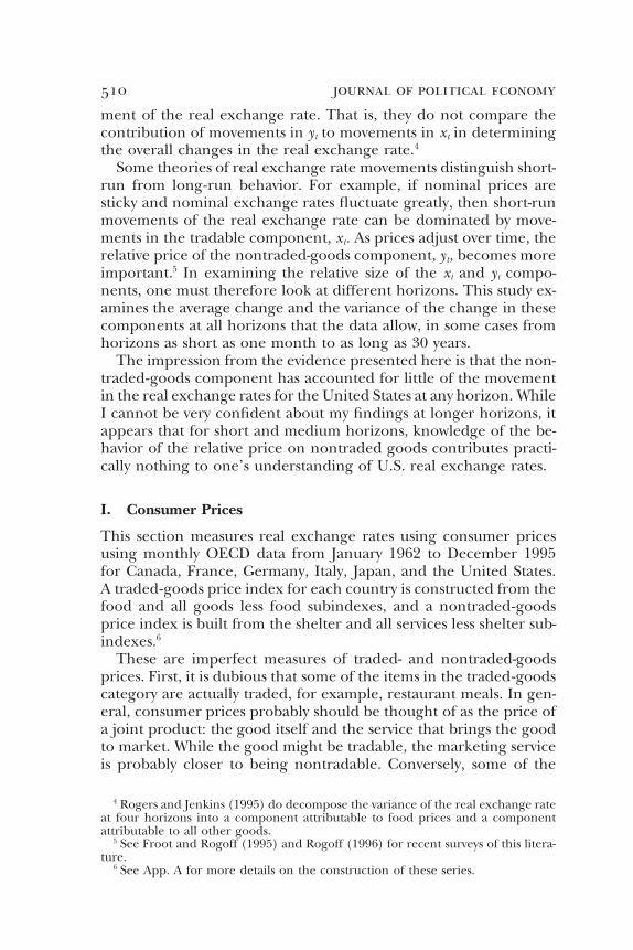
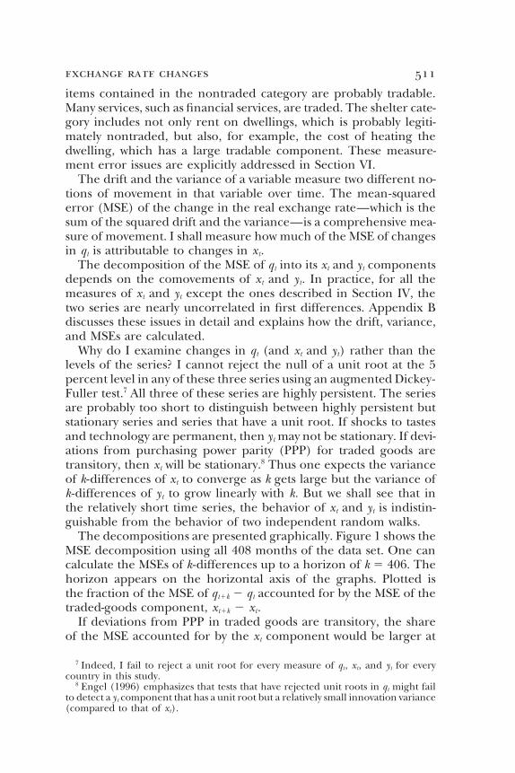
Fig. 1.—MSE decomposition: CPI data. MSE ratio estimates and 95 percent con-fidence intervals: MSE(xt1k 2 xt)/[MSE(xt1k 2 xt) 1 MSE(yt1k 2 yt)], January 1962to December 1995. a, Canadian/U.S. real exchange rate. b, Japanese/U.S. real ex-change rate. c, France, Germany, and Italy.
short horizons. So the lines plotted in the graphs should be declin-ing as the horizon increases. However, we should note that, at longhorizons, very few observations are used in the calculation of theMSE decomposition, so the statistic is not likely to be very reliable.
Figure 1 is striking in that it shows that the xt component (thetraded-goods component) accounts for nearly 100 percent of the
exchange rate changes 513
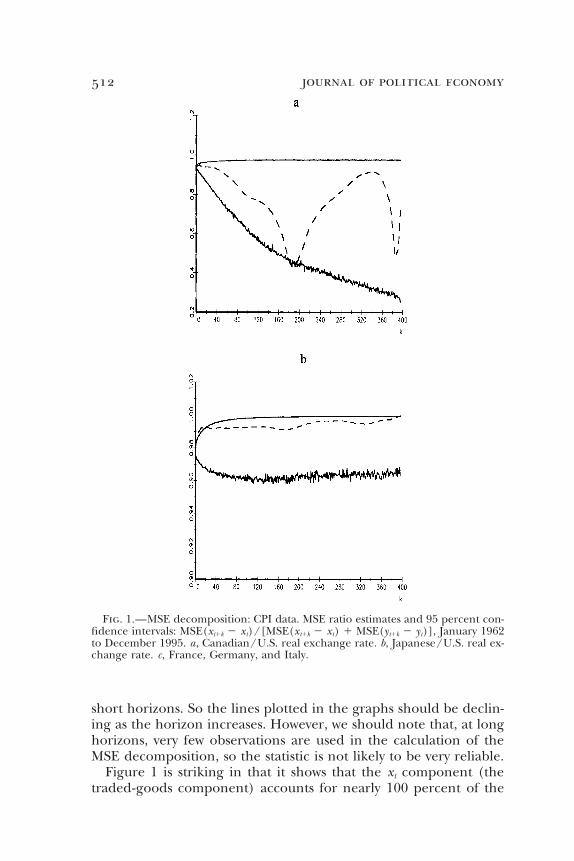
Fig. 1.—(Continued)
MSE of the U.S. real exchange rate changes at all horizons, for allrates except the Canadian-U.S. rate. It is notable that there is noapparent decline in the share of the MSE accounted for by xt evenas the horizon increases.
At short horizons for the Canadian-U.S. rate, the traded-goodscomponent accounts for over 95 percent of the movement; but asthe horizon increases, the importance of the xt component drops—to about 45 percent at the 15-year horizon—but the component be-gins to be more important again at horizons past 15 years. The longer-horizon numbers, however, are less reliable (although 168 monthlyobservations are available here to calculate the 20-year MSEs).
Figures 1a and 1b present 95 percent confidence intervals for thefraction of the MSE of qt1k 2 qt accounted for by the MSE of thetraded-goods component, xt1k 2 xt for the U.S.-Canadian (1a) andU.S.-Japanese (1b) real exchange rates. The confidence intervals arecalculated from Monte Carlo experiments (as described in App. B).The confidence intervals are calculated under the null that xt11 2 xt
and yt11 2 yt are independent, normally distributed random variableswith means and variances equal to their sample means and variances.
Note that the actual ratio is within the 95 percent confidence bandat all horizons. I can give a statistical interpretation of this result:one cannot reject the null that xt and yt are independent randomwalks. Thus there is nothing in the data that suggests that the impor-tance of the xt component in explaining movements in qt diminishesover time (or that the importance of the yt component increases).This should not be taken as conclusive evidence that the xt compo-nent is not stationary. With only 34 years of data, as I have already
514 journal of political economy
noted, one cannot develop conclusive evidence of the stationarityor nonstationarity of xt.
I do not present the confidence intervals for the real exchangerates of the United States relative to France, Germany, or Italy inorder to save space and have graphs that are legible. However, thesame results found in the Canadian and Japanese cases carry overto these real exchange rates: the fraction of the MSE of qt1k 2 qt
accounted for by the MSE of the traded-goods component lies withinthe 95 percent confidence interval at all horizons.
It is interesting to compare these findings with those of Kakkarand Ogaki (1994). These authors construct a yt variable and test forcointegration of that variable with qt. Their measures of yt and qt
correspond to the ones used in this paper in Sections III and IV.They find that they cannot reject the null that yt and qt are cointe-grated using Park’s (1990) test for the null of stochastic cointegra-tion. This finding holds for a number of different real U.S. exchangerates over a variety of time periods. If yt and qt are cointegrated, thenxt and yt cannot be independent random walks. But Kakkar andOgaki’s results are not necessarily inconsistent with the ones shownhere. I fail to reject the null that xt and yt are independent randomwalks, whereas they fail to reject the null that yt and qt are cointe-grated: both failures to reject likely reflect the low power of tests todistinguish between unit roots and stationarity in relatively shorttime spans.
The finding that over 95 percent of the MSE of the real exchangerate is accounted for by the MSE of the traded-goods componentholds if we examine the variance rather than the MSE for each ofthe real exchange rates. It is also the case that the drift in qt is almostentirely due to the drift in xt for all the real exchange rates exceptthe U.S.-Canadian rate. The portion of the drift of qt attributable tothe drift of xt is .485 for the U.S.-Canadian rate, .993 for the U.S.-French rate, .996 for the U.S.-German rate, .857 for the U.S.-Italianrate, and .999 for the U.S.-Japanese rate.
As Mussa (1986) and others have noted, the variance of the U.S.real exchange rate has been much lower in fixed nominal exchangerate periods than in floating exchange rate periods. Figure 1 usesdata from both fixed and floating periods for the United States. Onemight suspect that the results would look different from those fromjust the fixed-rate period, but that is not true. Figure 2a shows theMSE decomposition for the floating rate period, 1973–95, and fig-ure 2b shows the same decomposition for the fixed-rate period,1962–69. In both cases, at all horizons, nearly all of the movementin the real exchange rate comes from movements in the traded-goods component.
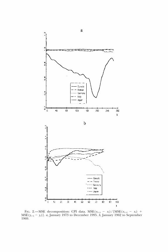
Fig. 2.—MSE decomposition: CPI data. MSE(xt1k 2 xt)/[MSE(xt1k 2 xt) 1MSE(yt1k 2 yt)]. a, January 1973 to December 1995. b, January 1962 to September1969.
516 journal of political economy
The fact that the traded-goods component accounts for nearlyall of the movement in real exchange rates even when the nominalexchange rate is fixed is reminiscent of the finding of Froot, Kim,and Rogoff (1995). Using 700 years of data, they find that the volatil-ity of deviations from the law of one price is no greater in the twenti-eth century under floating exchange rates than it was in previouscenturies when the exchange rate was essentially fixed.
II. Output Prices
This section uses output prices from the OECD’s international sec-toral database. Annual price indexes for 19 categories of output arecalculated by dividing nominal output figures by their real counter-parts.9 De Gregorio, Giovannini, and Wolf (1994) classify these sec-tors as tradable or nontradable using data on the export share intotal production. They conclude that all the commodities are trad-able. All services are categorized as nontradable, except for the trans-port, storage, and communication category. The traded and non-traded price indexes used here are constructed as in De Gregorio,Giovannini, and Wolf.
Although data are available for 14 countries, because of missingobservations, it was possible to construct long time series of real ex-change rates for only seven countries relative to the United States:Canada, Germany, Denmark, Finland, France, Japan, and Norway.The starting dates for these data vary from country to country. Insome cases the data start in 1960 (Finland, Germany, and the UnitedStates); in others the data begin as late as 1970 (France and Japan).The Norwegian data end in 1988, the U.S. and Canadian data endin 1989, and for the other countries the data end in 1990.
Figure 3 shows the MSE decomposition using all the data. Thesegraphs tell almost exactly the same story as figure 1 tells using con-sumer price data. At all horizons, for all countries with the exceptionof Canada, over 90 percent of the MSE of real exchange rate changesis accounted for by the MSE of the traded-goods component, xt.There is no tendency for this component to become less importantas the horizon lengthens.
As with the CPI data, for Canada the traded-goods share accountsfor a large share of real exchange rate movements at short horizons:
9 The sectors are agriculture; mining; food, beverages, and tobacco; textiles; woodand wood products; paper, printing, and publishing; chemicals; nonmetallic mineralproducts; basic metal products; machinery and equipment; other manufacturedproducts; electricity, gas, and water; construction; wholesale and retail trade; restau-rants and hotels; transport, storage, and communications; finance, insurance, andreal estate; community, social, and personal services; and government services.
exchange rate changes 517
over 80 percent of 1-year changes. This drops to around 50 percentat the 16-year horizon but then begins to rise again. Of course, veryfew observations are used to calculate the longer-horizon numbers.
Figures 3a and 3b show the confidence intervals for the fractionof the MSE of qt1k 2 qt accounted for by the MSE of the traded-goodscomponent, xt1k 2 xt, for the U.S.-Canadian and U.S.-Japanese realexchange rates, respectively. These confidence intervals are con-structed in the same way as those of the previous section. It is notablethat for Canada, the confidence intervals are very wide at the longerhorizons. As was the case in the previous section, the fraction ofthe MSE of qt1k 2 qt accounted for by the MSE of the traded-goodscomponent lies within the confidence bands at all horizons. Thiscan be interpreted as a failure to reject the hypothesis that xt and yt
are independent random walks. I have not shown the confidenceintervals for the other real exchange rates because of space consider-ations, but the same pattern holds true for them: the actual ratio ofthe MSE of the traded-goods component to the total MSE of thereal exchange rate lies within the confidence bands at all horizons.
As was true with the CPI data, the variance decompositions lookvery much like the MSE decompositions for all exchange rates. Forall countries except Canada, the traded-goods component also ac-counts for over 90 percent of the drift.
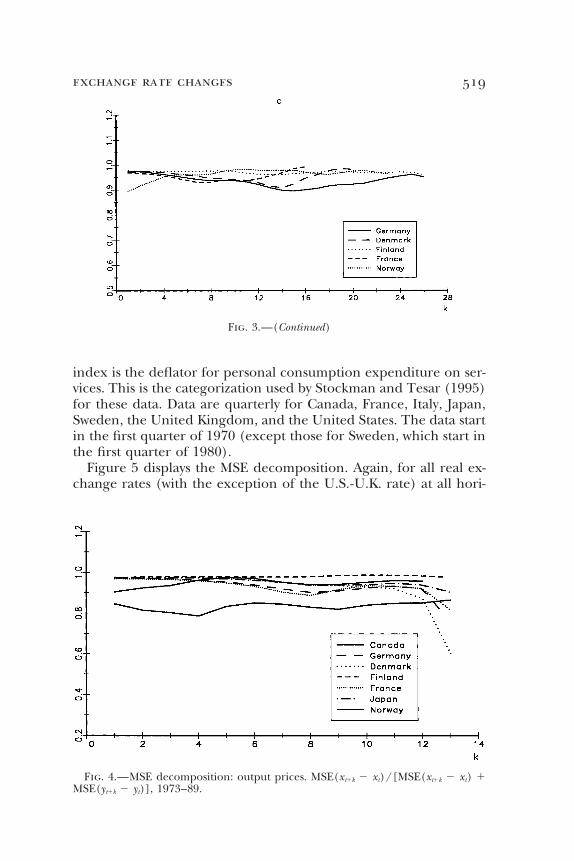
Figure 4 shows the MSE decomposition for the years 1973–89:the floating nominal exchange rate period. For all countries exceptCanada, the traded-goods component is responsible for over 95 per-cent of the MSE of the real exchange rate changes at all but thelongest horizons. For Canada, this fraction is around 85 percent forall horizons.
The CPI and output price data reach the same conclusion: thatvery little real exchange rate movements for the United States areattributable to the relative price of nontraded goods. This suggeststhat the results for the CPI data do not arise from the fact that con-sumer prices measure the price of both the tradable product and thenontradable service that brings the good to market. The marketingservice is much less important in the output price data, yet it showsthe same pattern as the CPI data.
III. Personal Consumption Deflators
This section uses data from national income accounts for personalconsumption deflators. The price indexes are constructed by divid-ing nominal consumption expenditures by real consumption expen-ditures. The traded-goods price index is the deflator for personalconsumption expenditure on commodities, whereas the nontraded
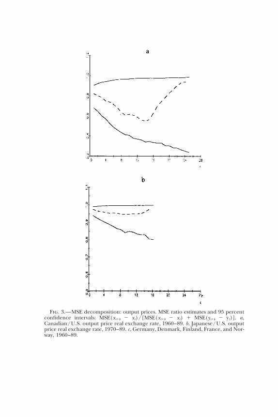
Fig. 3.—MSE decomposition: output prices. MSE ratio estimates and 95 percentconfidence intervals: MSE(xt1k 2 xt)/[MSE(xt1k 2 xt) 1 MSE(yt1k 2 yt)]. a,Canadian/U.S. output price real exchange rate, 1960–89. b, Japanese/U.S. outputprice real exchange rate, 1970–89. c, Germany, Denmark, Finland, France, and Nor-way, 1960–89.
exchange rate changes 519
Fig. 3.—(Continued)
index is the deflator for personal consumption expenditure on ser-vices. This is the categorization used by Stockman and Tesar (1995)for these data. Data are quarterly for Canada, France, Italy, Japan,Sweden, the United Kingdom, and the United States. The data startin the first quarter of 1970 (except those for Sweden, which start inthe first quarter of 1980).
Figure 5 displays the MSE decomposition. Again, for all real ex-change rates (with the exception of the U.S.-U.K. rate) at all hori-
Fig. 4.—MSE decomposition: output prices. MSE(xt1k 2 xt)/[MSE(xt1k 2 xt) 1MSE(yt1k 2 yt)], 1973–89.
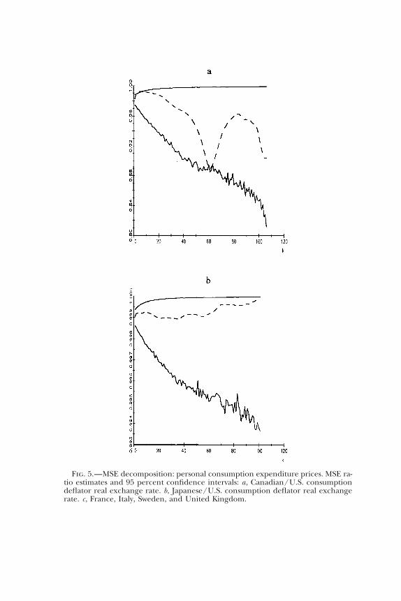
Fig. 5.—MSE decomposition: personal consumption expenditure prices. MSE ra-tio estimates and 95 percent confidence intervals: a, Canadian/U.S. consumptiondeflator real exchange rate. b, Japanese/U.S. consumption deflator real exchangerate. c, France, Italy, Sweden, and United Kingdom.
exchange rate changes 521
Fig. 5.—(Continued)
zons, the traded-goods component accounts for nearly all of themovement in the real exchange rate. For the U.S.-U.K. real ex-change rate, xt is responsible for over 95 percent of the movementout to 15 years. The fraction tails off to around 85 percent at the20-year horizon.
As in the previous two sections, I plot 95 percent confidence bandsfor the fraction of the MSE of qt1k 2 qt accounted for by the MSEof the traded-goods component for Canada (fig. 5a) and Japan (fig.5b). Again, these bands are computed under the null that xt11 2 xt
and yt11 2 yt are independent, normally distributed random variableswith means and variances equal to their sample means and variances.I find that for the two real exchange rates plotted, as well as for allthe other real exchange rates (whose confidence bands are not plot-ted because of space considerations), the sample value of the ratioof the MSE of the traded-goods component to the MSE of the realexchange rate lies within the 95 percent confidence interval at allhorizons.
IV. Producer Price Index
This section uses the overall PPI as an index of traded-goods prices.The traded-goods component, xt, is constructed as
xt 5 st 1 ln(PPI*t ) 2 ln(PPI t). (2)
The nontraded component, yt, is calculated as
yt 5 ln(CPI*t ) 2 ln(PPI*t ) 2 [ln(CPIt) 2 ln(PPI t)]. (3)
The data are monthly from January 1972 to late 1997 for 16 coun-
522 journal of political economy
tries: Austria, Belgium, Canada, Denmark, Finland, Germany,Greece, Italy, Japan, the Netherlands, Norway, Portugal, Spain, Swit-zerland, the United Kingdom, and the United States.10
This data set has the advantage that it covers many more countriesthan any of the others. However, there are at least four problemswith these data that seriously damage their worth.
1. Using the aggregate PPI as a measure of traded-goods prices iscrude. Clearly, some output is nontraded. Indeed, in Section II, Iuse only producer price data (from a different source) and classifysome sectors as tradable and some as nontradable.
2. In contrast to the other data, the measures of traded-goodsprices and nontraded-goods prices come from different surveys.Prices for similar goods might be measured in different ways in thetwo indexes. The PPI and CPI measures, for example, may have dif-ferent methods of averaging recordings of disparate prices for thesame good; they may survey different locations; they may adjust forchanges in quality differently, and so forth. There is no attempt toreconcile these differences, as there would be when prices all comefrom the same source.
3. Equation (3) allows us to construct an accurate measure of yt
only if the aggregate price index is a geometric average of traded-goods prices and nontraded-goods prices. However, the CPI (whichwe are using as the aggregate price index) is not constructed thisway. So even if the PPI were a good measure of traded-goods prices,equation (3) would not give us a good measure of yt.
4. In the previous sections, the decomposition of qt was uncompli-cated by worries of how to treat comovements of xt and yt becausethese two variables were nearly uncorrelated. But for the measuresin this section, xt and yt are negatively correlated. The reason is prob-ably that ln(PPI*t ) 2 ln(PPIt) appears with a positive sign in xt anda negative sign in yt. The decomposition of qt depends on how co-movements of xt and yt are handled in this case.
Figure 6 displays the decomposition of the MSE given by equation(B2) from Appendix B. Note that it is possible for xt to be responsiblefor more than 100 percent of the MSE of qt under this formula ifthe comovements of xt and yt are sufficiently negative. Formula (B2)arbitrarily classifies half of the comovements as being caused bychanges in xt and half as coming from changes in yt.
The general picture in figure 6 is that the xt component accountsfor over 70 percent of real exchange rate movements out to horizonsof 10 years. The Canadian and Belgian real exchange rates are minorexceptions because at some horizons less than 10 years the xt compo-
10 Portuguese and Italian data end in 1986 and 1985, respectively.
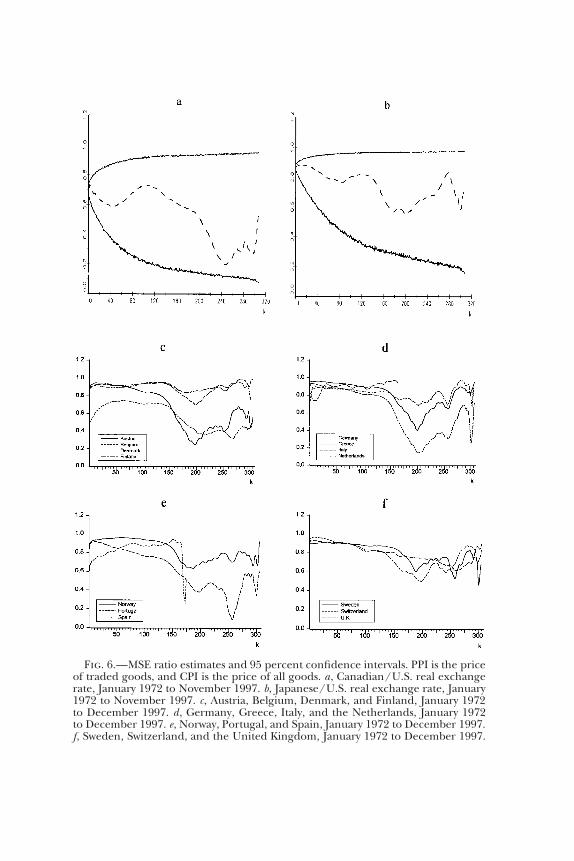
Fig. 6.—MSE ratio estimates and 95 percent confidence intervals. PPI is the priceof traded goods, and CPI is the price of all goods. a, Canadian/U.S. real exchangerate, January 1972 to November 1997. b, Japanese/U.S. real exchange rate, January1972 to November 1997. c, Austria, Belgium, Denmark, and Finland, January 1972to December 1997. d, Germany, Greece, Italy, and the Netherlands, January 1972to December 1997. e, Norway, Portugal, and Spain, January 1972 to December 1997.f, Sweden, Switzerland, and the United Kingdom, January 1972 to December 1997.
524 journal of political economy
nent is responsible for only around 60 percent of real exchange ratemovements. For most of the countries, xt determines greater than80 percent and in many cases greater than 90 percent of movementsin qt at horizons less than 10 years.
Figures 6a and 6b plot 95 percent confidence intervals for theU.S.-Canadian and U.S.-Japanese decompositions. As in the previ-ous sections, the sample value of the ratio of the MSE of the traded-goods component to the MSE of the real exchange rate lies withinthe 95 percent confidence interval at all horizons. These confidenceintervals are calculated under the null hypothesis that xt11 2 xt andyt11 2 yt are independent, normally distributed random variableswith means and variances equal to their sample means and variances.In contrast to the previous sections, the null is rejected at some hori-zons (particularly longer ones) for some currencies because, as Ihave already noted, xt and yt are negatively correlated. The decompo-sitions depicted in figures 6a–6 f will depend on how comovementsare treated for those countries.
V. The U.S.-Japanese Real Exchange Rate
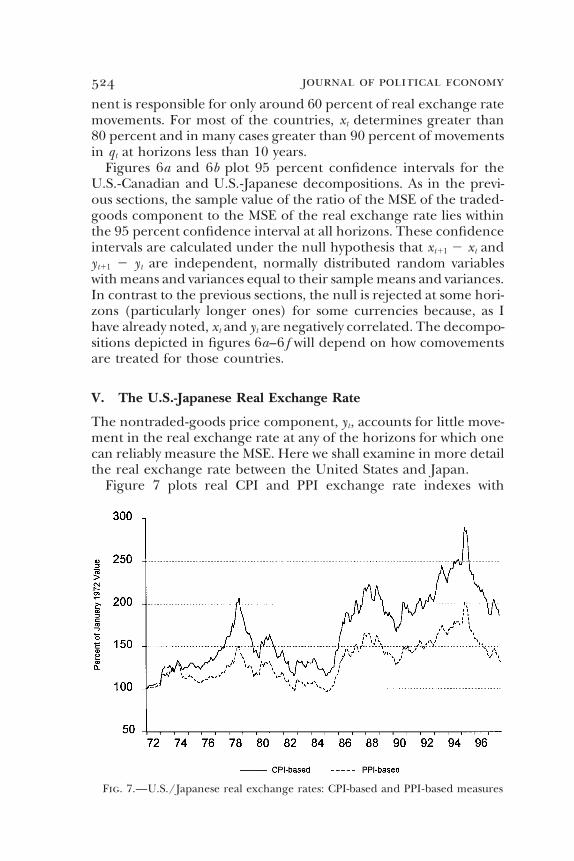
The nontraded-goods price component, yt, accounts for little move-ment in the real exchange rate at any of the horizons for which onecan reliably measure the MSE. Here we shall examine in more detailthe real exchange rate between the United States and Japan.
Figure 7 plots real CPI and PPI exchange rate indexes with
Fig. 7.—U.S./Japanese real exchange rates: CPI-based and PPI-based measures
exchange rate changes 525
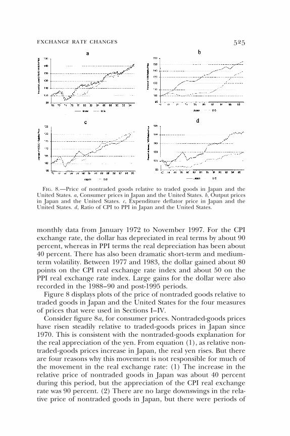
Fig. 8.—Price of nontraded goods relative to traded goods in Japan and theUnited States. a, Consumer prices in Japan and the United States. b, Output pricesin Japan and the United States. c, Expenditure deflator price in Japan and theUnited States. d, Ratio of CPI to PPI in Japan and the United States.
monthly data from January 1972 to November 1997. For the CPIexchange rate, the dollar has depreciated in real terms by about 90percent, whereas in PPI terms the real depreciation has been about40 percent. There has also been dramatic short-term and medium-term volatility. Between 1977 and 1983, the dollar gained about 80points on the CPI real exchange rate index and about 50 on thePPI real exchange rate index. Large gains for the dollar were alsorecorded in the 1988–90 and post-1995 periods.
Figure 8 displays plots of the price of nontraded goods relative totraded goods in Japan and the United States for the four measuresof prices that were used in Sections I–IV.
Consider figure 8a, for consumer prices. Nontraded-goods priceshave risen steadily relative to traded-goods prices in Japan since1970. This is consistent with the nontraded-goods explanation forthe real appreciation of the yen. From equation (1), as relative non-traded-goods prices increase in Japan, the real yen rises. But thereare four reasons why this movement is not responsible for much ofthe movement in the real exchange rate: (1) The increase in therelative price of nontraded goods in Japan was about 40 percentduring this period, but the appreciation of the CPI real exchangerate was 90 percent. (2) There are no large downswings in the rela-tive price of nontraded goods in Japan, but there were periods of
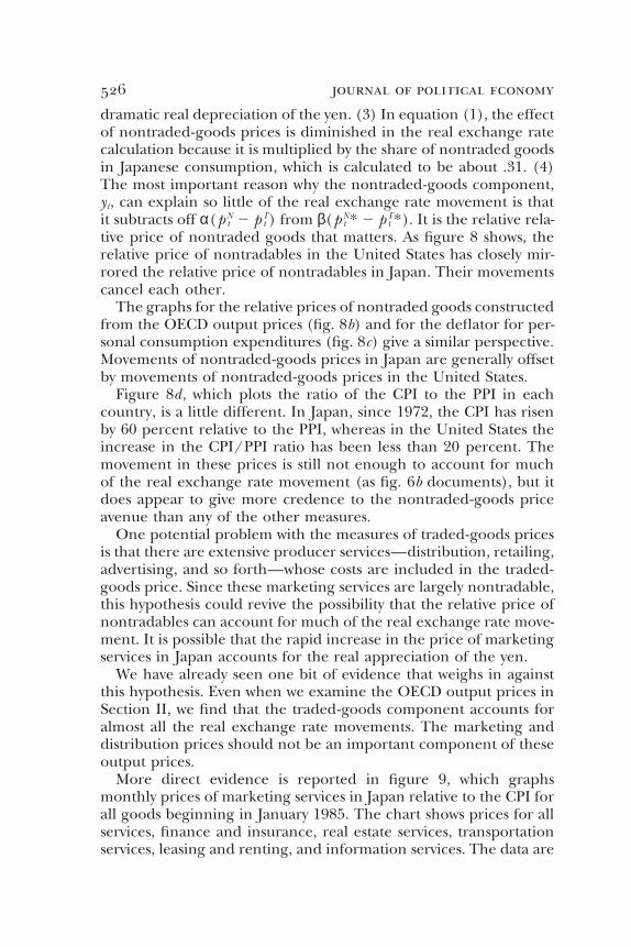
526 journal of political economy
dramatic real depreciation of the yen. (3) In equation (1), the effectof nontraded-goods prices is diminished in the real exchange ratecalculation because it is multiplied by the share of nontraded goodsin Japanese consumption, which is calculated to be about .31. (4)The most important reason why the nontraded-goods component,yt, can explain so little of the real exchange rate movement is thatit subtracts off α(p N
t 2 pTt ) from β(p N*t 2 pT*t ). It is the relative rela-
tive price of nontraded goods that matters. As figure 8 shows, therelative price of nontradables in the United States has closely mir-rored the relative price of nontradables in Japan. Their movementscancel each other.
The graphs for the relative prices of nontraded goods constructedfrom the OECD output prices (fig. 8b) and for the deflator for per-sonal consumption expenditures (fig. 8c) give a similar perspective.Movements of nontraded-goods prices in Japan are generally offsetby movements of nontraded-goods prices in the United States.
Figure 8d, which plots the ratio of the CPI to the PPI in eachcountry, is a little different. In Japan, since 1972, the CPI has risenby 60 percent relative to the PPI, whereas in the United States theincrease in the CPI/PPI ratio has been less than 20 percent. Themovement in these prices is still not enough to account for muchof the real exchange rate movement (as fig. 6b documents), but itdoes appear to give more credence to the nontraded-goods priceavenue than any of the other measures.
One potential problem with the measures of traded-goods pricesis that there are extensive producer services—distribution, retailing,advertising, and so forth—whose costs are included in the traded-goods price. Since these marketing services are largely nontradable,this hypothesis could revive the possibility that the relative price ofnontradables can account for much of the real exchange rate move-ment. It is possible that the rapid increase in the price of marketingservices in Japan accounts for the real appreciation of the yen.
We have already seen one bit of evidence that weighs in againstthis hypothesis. Even when we examine the OECD output prices inSection II, we find that the traded-goods component accounts foralmost all the real exchange rate movements. The marketing anddistribution prices should not be an important component of theseoutput prices.
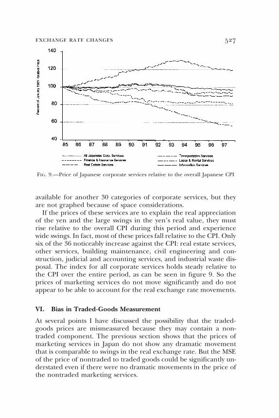
More direct evidence is reported in figure 9, which graphsmonthly prices of marketing services in Japan relative to the CPI forall goods beginning in January 1985. The chart shows prices for allservices, finance and insurance, real estate services, transportationservices, leasing and renting, and information services. The data are
exchange rate changes 527
Fig. 9.—Price of Japanese corporate services relative to the overall Japanese CPI
available for another 30 categories of corporate services, but theyare not graphed because of space considerations.
If the prices of these services are to explain the real appreciationof the yen and the large swings in the yen’s real value, they mustrise relative to the overall CPI during this period and experiencewide swings. In fact, most of these prices fall relative to the CPI. Onlysix of the 36 noticeably increase against the CPI: real estate services,other services, building maintenance, civil engineering and con-struction, judicial and accounting services, and industrial waste dis-posal. The index for all corporate services holds steady relative tothe CPI over the entire period, as can be seen in figure 9. So theprices of marketing services do not move significantly and do notappear to be able to account for the real exchange rate movements.
VI. Bias in Traded-Goods Measurement
At several points I have discussed the possibility that the traded-goods prices are mismeasured because they may contain a non-traded component. The previous section shows that the prices ofmarketing services in Japan do not show any dramatic movementthat is comparable to swings in the real exchange rate. But the MSEof the price of nontraded to traded goods could be significantly un-derstated even if there were no dramatic movements in the price ofthe nontraded marketing services.
528 journal of political economy
Suppose, in fact, that nontraded marketing services are perfectlycorrelated with the measure of other nontraded-goods prices, p N
t .But the measure of traded-goods prices, pT
t , is actually a weightedaverage of the nontraded-goods price and the price of goods thatare truly traded, p C
t :
p Tt 5 γpN
t 1 (1 2 γ)p Ct .
Likewise, in the foreign country, γ is the weight that nontraded mar-keting services take in the measure of traded-goods prices.
In this case, the weight that nontraded goods receive in the overallprice index domestically is actually α 1 γ(1 2 α), whereas I havetaken it to be just α. The true measure of yt that one would like is
y t 5 [β 1 γ(1 2 β)](pN*t 2 pC*t ) 2 [α 1 γ(1 2 α)](pNt 2 p C
t ).
Since I actually use yt, there is bias in the measure of y t. We canwrite yt as
yt 5 β(1 2 γ)(p N*t 2 pC*t ) 2 α(1 2 γ)(p Nt 2 pC
t ).
While the domestic relative price of nontraded goods should be get-ting a weight of α 1 γ(1 2 α) as in the expression for yt (and β 1γ(1 2 β) for foreign goods), we are actually giving them a weightof α(1 2 γ) (and β(1 2 γ) for foreign goods) when we use yt as ourmeasure. This biases downward the importance of the relative priceof nontraded goods. When γ is large, the bias could be severe.
The problem is that we do not measure pCt and pC*t directly. We
shall, however, construct measures by using the relation
p Ct 5
11 2 γ
(pTt 2 γp N
t ). (4)
The value of γ is unknown, but we shall experiment with differentvalues. We can use this measure of p C
t (and the analogous measurefor p C*t ) to get a measure of yt.
Before proceeding in this direction, note that this calculation gen-erates a series for y t that is too volatile. We have assumed that theprice of marketing services is perfectly correlated with pN
t . Supposeinstead that p N
t measures the price of marketing services, pMSt , with
measurement error ut :
p MSt 5 p N
t 1 ut,
and likewise for the foreign country. Ideally, y t would be measuredas a weighted average of the relative prices of pN
t and pMSt to p C
t :
exchange rate changes 529
β(pN*t 2 p C*t ) 1 γ(1 2 β)(pMS*t 2 pC*t ) 2 α(pNt 2 pC
t )
2 γ(1 2 α)(p MSt 2 p C
t ).
But when measurement error is introduced into pMSt , our measure
of y t is actually
β(p N*t 2 pC*t ) 1 γ(1 2 β)(p MS*t 2 p C*t ) 2 α(pNt 2 p C
t )
2 γ(1 2 α)(pMSt 2 pC
t ) 1γ
1 2 γ(u t 2 u*t ).
This introduces volatility into our measure of yt that can be substan-tial when γ is large.
With this caveat in mind, note that using equation (4) (and itsequivalent for pC*t ), we can write y t in terms of variables that aremeasurable:
y t 5 1β 1γ
1 2 γ2 (pN*t 2 p T*t ) 2 1α 1γ
1 2 γ2 (p Nt 2 pT
t ).
So we can take our previous measure of yt and simply increase theweights from β and α to β 1 [γ/(1 2 γ)] and α 1 [γ/(1 2 γ)].
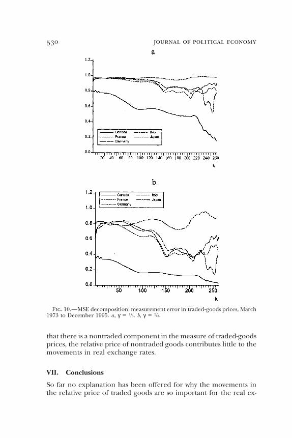
Figure 10 reproduces the MSE decomposition using CPIs over thefloating exchange rate period that was presented in figure 2. How-ever, the weights on the relative prices of nontraded goods havebeen increased. In figure 10a, γ is set to 1/3 (which means that 0.5is added to β and α).11 This choice of γ is arbitrary. Its interpretationis that the share of marketing services in the final-goods prices is 1/3.We see that the fraction of the MSE attributable to the traded-goodscomponent, xt, is lower than in figure 2. However, it is still very large:xt accounts for over 90 percent at all but the longest horizons exceptfor the U.S.-Canadian real exchange rate.
Figure 10b uses a value of γ equal to 2/3 (which means that 2.0is added to β and α). Both because of the measurement problemsintroduced into our measure of yt that overstate its volatility and be-cause the marketing share is unlikely to be as large as 2/3, the num-bers presented in figure 10b are probably a lower bound on the shareof the MSE of qt1k 2 qt accounted for by the MSE of the traded-goods component, xt1k 2 xt. Even so, the traded-goods component isresponsible for a large share, especially at short to medium horizons.
I conclude that even when one takes into account the possibility
11 The term s 1 p T*t 2 p Tt is used in constructing xt rather than s 1 pC*t 2 p C
t .Because pT*t 2 p T
t is less volatile than p C*t 2 p Ct , fig. 10 biases down the contribution
of the xt component.
530 journal of political economy
Fig. 10.—MSE decomposition: measurement error in traded-goods prices, March1973 to December 1995. a, γ 5 1/3. b, γ 5 2/3.
that there is a nontraded component in the measure of traded-goodsprices, the relative price of nontraded goods contributes little to themovements in real exchange rates.
VII. Conclusions
So far no explanation has been offered for why the movements inthe relative price of traded goods are so important for the real ex-
exchange rate changes 531
change rate. One possibility is terms-of-trade movements. If thereare fluctuations in the relative prices of goods that constitute thetraded-goods price indexes and if the weights these goods receiveare different in the U.S. and foreign price indexes, then the relativetraded-goods price indexes will fluctuate.
It is difficult to investigate this avenue with my data since one can-not disaggregate the traded-goods price indexes much. With theconsumer price data, the indexes are composed from only two sub-indexes: for food and for all goods not including food. For theOECD price data, the traded-goods price index is composed of sub-indexes for 12 categories of goods and services. None of the othertraded-goods price indexes can be disaggregated.
Appendix C reports the outcome of investigating the terms-of-trade hypothesis for the CPI and OECD output price indexes. There,I find that this hypothesis explains very little because the weights ofthe subcategories in the overall price indexes are not too differentacross countries. So even if there is a lot of volatility in relative pricemovements among the subcategories, it does not have much of aneffect on the overall relative price.
It should be noted that all the real exchange rates examined inthis study pertain to high-income countries. As table 3 of Rogoff(1996) demonstrates, the behavior of real exchange rates for low-income countries might be very different. The absolute purchasingpower of the currencies of low-income countries is much higherthan for high-income countries, although within the two groupsthere seems to be little relationship between income and purchasingpower. It seems likely that the disparity between low-income andhigh-income countries’ purchasing powers reflects differences inthe relative prices of nontraded goods.
It is tempting to attribute the movements in the traded-goodsprice indexes to failures of the law of one price. That conclusionwould be consistent with the findings of a number of recent studies(Engel 1993; Froot et al. 1995; Rogers and Jenkins 1995; Engel andRogers 1996, 1998; Knetter 1997). However, there are many issues tobe resolved in that area: What determines export prices to differentregions from the same country? How important is pricing to marketin determining real exchange rate movements? What systematic rela-tionship is there between the price of a good at the port and at theconsumer outlet? To what extent do the degree of product differen-tiation and the competitiveness of the industry determine differ-ences in prices between locations? What role does nominal pricestickiness play, and how is it related to these other questions? Thekey to understanding real exchange rate movements may be found
532 journal of political economy
in the answers to these questions. But the evidence of this papersuggests that the relative price of nontraded goods has little importfor understanding U.S. real exchange rate movements over the shortand medium run.
Finally, it should be emphasized that this study cannot shed lighton the importance of the relative price of nontraded goods in de-termining the real exchange rate in the long run. Engel (1996), infact, argues that nontraded-goods prices could have a large impacton real exchange rates at long horizons. In that study, a simplemodel for the U.S.-U.K. real exchange rate is calibrated (using thedata from Sec. III of this paper) in which the yt component is nonsta-tionary and xt is stationary. At horizons of 100 years, the yt compo-nent accounts for about half of the variance of the real exchangerate. Yet, using Monte Carlo exercises, I find that one is very likelyto conclude that the real exchange rate is stationary. That is, evenin 100 years of data I cannot detect the nonstationary yt component.Inference about the presence of a unit root component is difficultbecause the stationary xt variable has such a high variance that itmasks the movements in the nonstationary yt variable. Certainly inthe 20–30-year samples used in this paper, one would not be ableto discern whether nontraded-goods prices had a significant influ-ence on real exchange rate movements in the very long run.
Appendix A
Data
Nominal exchange rates are taken from Datastream. Period average ex-change rates from the International Monetary Fund’s International Finan-cial Statistics database are used for 1972–97. In general, monthly price in-dexes are constructed from averages of prices observed throughout themonth. So monthly average exchange rates are appropriate: rates measuredat a point in time would overstate the volatility of exchange rates comparedto prices. For 1969–71, exchange rates are period averages from Data-stream’s national government series. End-of-period exchange rates fromthe OECD database are used for 1960–69. Since exchange rates are gener-ally fixed in this period, there is little difference between period averagesand end-of-period rates.
Seasonally unadjusted monthly data from January 1972 to December1995 on consumer prices are used in Section I. The data are taken fromDatastream’s OECD database on all items (AI ), all goods less food (AGLF ),food (F ), services less rent (SLR ), and rent (R ). The weights in the priceindex are constructed from the regression
∆(ai 2 r) 5 φ1∆(aglf 2 r) 1 φ2 ∆( f 2 r) 1 φ3 ∆(slr 2 r) 1 e,
exchange rate changes 533
where ∆ is the first-difference operator, and lowercase letters are used todenote natural logarithms. Then I construct
pT 5 1 φ1
φ1 1 φ22 ⋅ aglf 1 1 φ2
φ1 1 φ22 ⋅ f
and
pN 5 1 φ3
1 2 φ1 2 φ22 ⋅ slr 1 11 2 φ1 2 φ2 2 φ3
1 2 φ1 2 φ22 ⋅ r .
Section II constructs price indexes for each of 19 sectors as the ratio ofnominal to real output, measured annually, taken from the OECD’s inter-national sectoral database. The nontraded- and traded-goods price indexesare weighted averages of the price indexes of each sector; the weights arefixed and taken as the average share of each sector’s output in total output.The data ranges are Canada, 1961–89; Germany, 1960–90; Denmark, 1966–90; Finland, 1960–90; France, 1970–90; Japan, 1970–90; Norway, 1962–88;and United States, 1960–89.
The prices in Section III are personal consumption deflators from Data-stream’s OECD quarterly accounts. The data ranges for Canada, France,and the United Kingdom are 1970:1–1997:1; for the United States, 1970:1–1997:2; for Japan, 1970:1–1996:1; for Italy, 1970:1–1995:3; and for Sweden,1980:1–1994:2. Price indexes are computed as the ratio of nominal to realexpenditures, with commodities classified as traded goods and services asnontraded. The data for Canada, France, Italy, and the United States wereseasonally adjusted. For Japan and Sweden they were unadjusted, but wereadjusted using a multiplicative seasonal adjustment.
In contrast to all the other price data used in this study, these prices areseasonally adjusted. This is likely to make the traded-goods component, xt,relatively more important in explaining short-term movements in qt. Sea-sonal adjustment tends to smooth the price series over short intervals. Butxt also contains the nominal exchange rate, which is not seasonally adjusted,so xt will be relatively more volatile.
Section IV uses monthly, not seasonally adjusted, producer and consumerprice indexes from Datastream’s International Monetary Fund series withfour exceptions. The Belgian, German, and Norwegian producer price se-ries and the Italian consumer price series were taken from Datastream’snational account data. All data begin in January 1972. The data for Ger-many and the United States end in 1997:12; Canada, Japan, the Nether-lands, Norway, Spain, and Switzerland, in 1997:11; the United Kingdom,1997:10; Sweden, 1997:9; Finland, 1997:7; Portugal, 1986:12; and Italy,1985:12.
The prices of corporate services used in Section V are taken from Data-stream’s national government series. The data are monthly from January1985 to November 1997, not seasonally adjusted.
Nontraded goods’ weight in the price indexes of Sections I–III are shownin table A1.
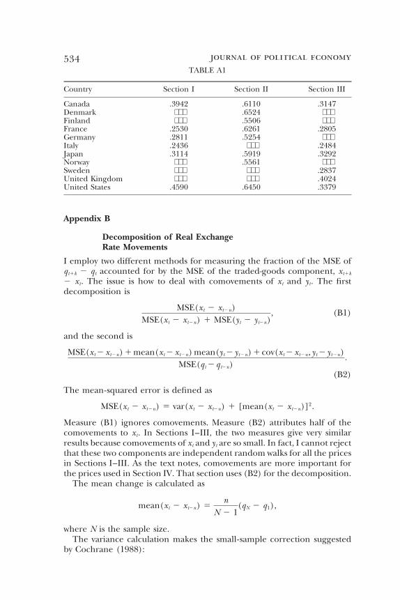
534 journal of political economyTABLE A1
Country Section I Section II Section III
Canada .3942 .6110 .3147Denmark ⋅ ⋅ ⋅ .6524 ⋅ ⋅ ⋅Finland ⋅ ⋅ ⋅ .5506 ⋅ ⋅ ⋅France .2530 .6261 .2805Germany .2811 .5254 ⋅ ⋅ ⋅Italy .2436 ⋅ ⋅ ⋅ .2484Japan .3114 .5919 .3292Norway ⋅ ⋅ ⋅ .5561 ⋅ ⋅ ⋅Sweden ⋅ ⋅ ⋅ ⋅ ⋅ ⋅ .2837United Kingdom ⋅ ⋅ ⋅ ⋅ ⋅ ⋅ .4024United States .4590 .6450 .3379
Appendix B
Decomposition of Real ExchangeRate Movements
I employ two different methods for measuring the fraction of the MSE ofqt1k 2 qt accounted for by the MSE of the traded-goods component, xt1k
2 xt. The issue is how to deal with comovements of xt and yt. The firstdecomposition is
MSE(xt 2 xt2n)MSE(xt 2 xt2n) 1 MSE(yt 2 yt2n)
, (B1)
and the second is
MSE(xt 2 xt2n) 1 mean(xt 2 xt2n) mean(yt 2 yt2n) 1 cov(xt 2 xt2n, yt 2 yt2n)MSE(qt 2 qt2n)
.
(B2)
The mean-squared error is defined as
MSE(xt 2 xt2n) 5 var(xt 2 xt2n) 1 [mean(xt 2 xt2n)]2.
Measure (B1) ignores comovements. Measure (B2) attributes half of thecomovements to xt. In Sections I–III, the two measures give very similarresults because comovements of xt and yt are so small. In fact, I cannot rejectthat these two components are independent random walks for all the pricesin Sections I–III. As the text notes, comovements are more important forthe prices used in Section IV. That section uses (B2) for the decomposition.
The mean change is calculated as
mean(xt 2 xt2n) 5n
N 2 1(qN 2 q1),
where N is the sample size.The variance calculation makes the small-sample correction suggested
by Cochrane (1988):
exchange rate changes 535
var(xt 2 xt2n) 5N
(N 2 n 2 1)(N 2 n) ^N2n
j51
[xj1n 2 xj 2 mean (xj1n 2 xj)]2.
A small-sample correction would not be needed for a variance decomposi-tion since the bias correction would cancel out in the numerator and de-nominator of the decomposition. But the MSE decomposition would over-emphasize the squared drift if a downward-biased measure of the variancewere used.
To construct confidence intervals, I first calculate the sample mean andvariance of xt11 2 xt and yt11 2 yt. Then 5,000 artificial series of length N2 1 of xt11 2 xt and yt11 2 yt are created using the normal random numbergenerator (rndn) on Gauss with mean and variance equal to those of thedata. These are cumulated to create artificial series of xt and yt, which arenow, by construction, independent random walks. Then the n th differencesof these series are taken, and the MSE decompositions recorded. The con-fidence intervals exclude the largest 125 and smallest 125 ratios that arecalculated. This process is repeated to get the confidence interval at eachof the n horizons. (New artificial series are created for the calculations ateach horizon because the computer program would be inefficient if it hadto save all 5,000 series to do the calculations at each horizon.)
Appendix C
Terms-of-Trade Movements
This Appendix briefly addresses the issue of why movements in the relativeprice of traded goods are so large. One possibility is that the law of oneprice fails. Another possibility is that the traded-goods price indexes weightgoods differently in the two countries. Suppose that
p Tt 5 νp 1
t 1 (1 2 ν)p 2t
and
pT*t 5 ηp 1*t 1 (1 2 η)p 2*t .
Even if the law of one price held for each good, so p jt 5 st 1 p j*t ( j 5 1,
2), if ν ≠ η, then pTt 2 st 2 p T*t will change as p 1
t moves relative to p 2t .
To gauge the importance of this possibility, I recalculate the foreigntraded-goods price index using U.S. weights to see whether this significantlylowers the MSE of pT
t 2 st 2 p T*t . If terms-of-trade movements were impor-tant, the MSE should decline under this recalculation. In fact, the MSE(and the squared drift and variance) does not decline. The same is true forthe opposite tack of calculating the U.S. price index using foreign weights.
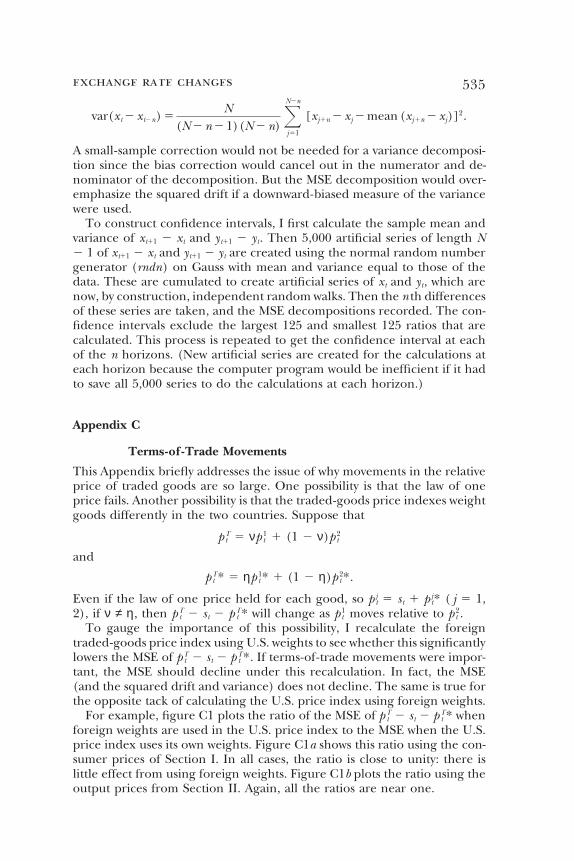
For example, figure C1 plots the ratio of the MSE of p Tt 2 st 2 p T*t when
foreign weights are used in the U.S. price index to the MSE when the U.S.price index uses its own weights. Figure C1a shows this ratio using the con-sumer prices of Section I. In all cases, the ratio is close to unity: there islittle effect from using foreign weights. Figure C1b plots the ratio using theoutput prices from Section II. Again, all the ratios are near one.
536 journal of political economy
Fig. C1.—MSE effect of variation in the terms of trade. a, CPI prices, January1962 to December 1995. b, Output prices, 1960–89.
References
Asea, Patrick K., and Mendoza, Enrique G. ‘‘The Balassa-Samuelson Model:A General-Equilibrium Appraisal.’’ Rev. Internat. Econ. 2 (October 1994):244–67.
Brock, Philip L. ‘‘Economic Development and the Relative Price of Non-tradables: Global Dynamics of the Krueger-Deardorff-Leamer Model.’’Rev. Internat. Econ. 2 (October 1994): 268–83.
Brock, Philip L., and Turnovsky, Stephen J. ‘‘The Dependent-EconomyModel with Both Traded and Nontraded Capital Goods.’’ Rev. Internat.Econ. 2 (October 1994): 306–25.
Canzoneri, Matthew B.; Cumby, Robert E.; and Diba, Behzad. ‘‘RelativeLabor Productivity and the Real Exchange Rate in the Long Run: Evi-

exchange rate changes 537dence for a Panel of OECD Countries.’’ Working Paper no. 5676. Cam-bridge, Mass.: NBER, July 1996.
Cochrane, John H. ‘‘How Big Is the Random Walk in GNP?’’ J.P.E. 96 (Oc-tober 1988): 893–920.
De Gregorio, Jose; Giovannini, Alberto; and Krueger, Thomas H. ‘‘The Be-havior of Nontradable-Goods Prices in Europe: Evidence and Interpreta-tion.’’ Rev. Internat. Econ. 2 (October 1994): 284–305.
De Gregorio, Jose; Giovannini, Alberto; and Wolf, Holger C. ‘‘InternationalEvidence on Tradables and Nontradables Inflation.’’ European Econ. Rev.38 (June 1994): 1225–44.
De Gregorio, Jose, and Wolf, Holger C. ‘‘Terms of Trade, Productivity, andthe Real Exchange Rate.’’ Working Paper no. 4807. Cambridge, Mass.:NBER, July 1994.
Engel, Charles. ‘‘Real Exchange Rates and Relative Prices: An EmpiricalInvestigation.’’ J. Monetary Econ. 32 (August 1993): 35–50.
———. ‘‘Long-Run PPP May Not Hold after All.’’ Working Paper no. 5646.Cambridge, Mass.: NBER, July 1996.
Engel, Charles, and Rogers, John H. ‘‘How Wide Is the Border?’’ A.E.R. 86(December 1996): 1112–25.
———. ‘‘Regional Patterns in the Law of One Price: The Roles of Geogra-phy versus Currencies.’’ In Regionalization of the World Economy, edited byJeffrey A. Frankel. Chicago: Univ. Chicago Press, 1998.
Froot, Kenneth A.; Kim, Michael; and Rogoff, Kenneth. ‘‘The Law of OnePrice over 700 Years.’’ Working Paper no. 5132. Cambridge, Mass.: NBER,May 1995.
Froot, Kenneth A., and Rogoff, Kenneth. ‘‘Perspectives on PPP and Long-Run Real Exchange Rates.’’ In Handbook of International Economics, vol. 3,edited by Gene M. Grossman and Kenneth Rogoff. Amsterdam: North-Holland, 1995.
Kakkar, Vikas, and Ogaki, Masao. ‘‘Real Exchange Rates and Nontrad-ables.’’ Working Paper no. 379. Rochester, N.Y.: Univ. Rochester, CenterEcon. Res., 1994.
Knetter, Michael M. ‘‘Why Are Retail Prices in Japan So High? Evidencefrom German Export Prices.’’ Internat. J. Indus. Organization 15 (August1997): 549–72.
Marston, Richard C. ‘‘Real Exchange Rates and Productivity Growth in theUnited States and Japan.’’ In Real-Financial Linkages among Open Econo-mies, edited by Sven W. Arndt and J. David Richardson. Cambridge, Mass.:MIT Press, 1987.
Mussa, Michael. ‘‘Nominal Exchange Rate Regimes and the Behavior ofReal Exchange Rates: Evidence and Implications.’’ Carnegie-RochesterConf. Ser. Public Policy 25 (Autumn 1986): 117–213.
Obstfeld, Maurice, and Rogoff, Kenneth. Foundations of International Macro-economics. Cambridge, Mass.: MIT Press, 1996.
Park, Joon Y. ‘‘Testing for Unit Roots and Cointegration by Variable Addi-tion.’’ In Advances in Econometrics, vol. 8, edited by Thomas B. Fomby andGeorge F. Rhodes, Jr. Greenwich, Conn.: JAI, 1990.
Razin, Assaf. ‘‘The Dynamic-Optimizing Approach to the Current Account:Theory and Evidence.’’ In Understanding Interdependence: The Macroeconom-ics of the Open Economy, edited by Peter B. Kenen. Princeton, N.J.:Princeton Univ. Press, 1995.
Rogers, John H., and Jenkins, Michael. ‘‘Haircuts or Hysteresis? Sources ofMovements in Real Exchange Rates.’’ J. Internat. Econ. 38 (May 1995):339–60.

538 journal of political economy
Rogoff, Kenneth. ‘‘The Purchasing Power Parity Puzzle.’’ J. Econ. Literature34 (June 1996): 647–68.
Samuelson, Paul A. ‘‘Facets of Balassa-Samuelson Thirty Years Later.’’ Rev.Internat. Econ. 2 (October 1994): 201–26.
Stockman, Alan C., and Tesar, Linda L. ‘‘Tastes and Technology in a Two-Country Model of the Business Cycle: Explaining International Comove-ments.’’ A.E.R. 85 (March 1995): 168–85.


![Staff Accounting Bulletin 107 - IAS Plus · SECURITIES AND EXCHANGE COMMISSION 17 CFR PART 211 [Release No. SAB 107] Staff Accounting Bulletin No. 107 AGENCY: Securities and Exchange](https://img.pdfslide.us/doc/110x75/603af229ec6be073b9010d47/staff-accounting-bulletin-107-ias-plus-securities-and-exchange-commission-17-cfr.jpg)