NBER WORKING PAPER SERIES

ACCOUNTING FOR THE RISE IN CONSUMER BANKRUPTCIES

Igor LivshitsJames MacGeeMichèle Tertilt

Working Paper 13363http://www.nber.org/papers/w13363

NATIONAL BUREAU OF ECONOMIC RESEARCH1050 Massachusetts Avenue

Cambridge, MA 02138September 2007

We thank Kartik Athreya, Satyajitt Chatterjee, Huberto Ennis, Martin Gervais, Jeremy Greenwood,Karen Pence, Jose-Victor Rios-Rull, Stephen Zeldes and seminar participants at the 2005 PhiladelphiaFed Consumer Credit & Payments conference, November 2005 NBER ME conference, the SITE 2004conference, the 2003 Western-Toronto Macro conference, the SED Meetings in Paris and Florence,the Federal Reserve Banks of Minneapolis, Richmond, and Chicago, the Bank of Canada, the EuropeanCentral Bank, and UC Davis, Illinois, Iowa, New Brunswick, Pennsylvania, Rochester, Texas-Austin,Wharton, York and Queen's Universities for helpful comments. Livshits acknowledges financial supportfrom the Arts, Humanities & Social Sciences Fund of the UWO. Livshits and MacGee acknowledgefinancial support from SSHRCC and from the Economic Policy Research Institute. Tertilt is gratefulto financial support from NSF grant No. 0519324. We would like to thank Jie Zhou for excellent researchassistance. The views expressed herein are those of the author(s) and do not necessarily reflect theviews of the National Bureau of Economic Research.

© 2007 by Igor Livshits, James MacGee, and Michèle Tertilt. All rights reserved. Short sections oftext, not to exceed two paragraphs, may be quoted without explicit permission provided that full credit,including © notice, is given to the source.

Accounting for the Rise in Consumer BankruptciesIgor Livshits, James MacGee, and Michèle TertiltNBER Working Paper No. 13363September 2007JEL No. E21,E44,G18,K35

ABSTRACT

Personal bankruptcies in the United States have increased dramatically, rising from 1.4 per thousandworking age population in 1970 to 8.5 in 2002. We use a heterogeneous agent life-cycle model withcompetitive financial intermediaries who can observe households' earnings, age and current asset holdingsto evaluate several commonly offered explanations. We find that increased uncertainty (income shocks,expense uncertainty) cannot quantitatively account for the rise in bankruptcies. Instead, the rise infilings appears to mainly reflect changes in the credit market environment. We find that credit marketinnovations which cause a decrease in the transactions cost of lending and a decline in the cost of bankruptcycan largely accounting for the rise in consumer bankruptcy. We also argue that the abolition of usurylaws and other legal changes are unimportant.

Igor LivshitsDepartment of EconomicsUniversity of Western OntarioSocial Science CentreLondon, Ontario N6A5C2livshits@uwo.ca

James MacGeeDepartment of EconomicsUniversity of Western OntarioLondon, Ontario Canada NCA 5C2jmacgee@uwo.ca

Michèle TertiltDepartment of EconomicsStanford University579 Serra MallStanford, CA 94305-6072and NBERtertilt@stanford.edu

1 Introduction

The past thirty years have witnessed an explosive growth in the number of consumer

bankruptcy filings in the United States. Personal bankruptcies have increased from

1.4 per thousand of the working age population in 1970 to 8.5 in 2002 (see Figure 1),

with virtually all of the increase occurring between 1980 and 2000. This dramatic rise

in bankruptcies has motivated a large literature on potential explanations. Somewhat

surprisingly, little effort has been made to understand the quantitative implications

of these explanations. In this paper, we address this void and quantitatively eval-

uate the most commonly offered explanations of the dramatic increase in consumer

bankruptcies.

These potential explanations can be grouped into two categories: (i)“uncertainty”

has increased leading to an increased number of households in financial trouble or

(ii) changes in the credit market environment have made bankruptcy more attractive

or expanded households’ access to credit. The “uncertainty” category includes three

stories. The first two stories involve an increase in idiosyncratic uncertainty at the

household level, due to increased labor earnings volatility or an increase in the number

of U.S. households without medical insurance (Barron, Elliehausen, and Staten (2000)

and Warren and Warren Tyagi (2003)). The third story we consider argues that

compositional changes in the population – the passing of the baby-boomers through

the prime bankruptcy ages and changing family structure – have increased the number

of risky households (Sullivan, Warren, and Westbrook (2000)).

The second category includes three possible channels via which changes in the

credit market environment could significantly influence households incentives to bor-

row and file for bankruptcy. Perhaps the most common explanation of the rise in

bankruptcies is that the cost of filing for bankruptcy has declined (e.g., Gross and

Souleles (2002)). A frequently heard version of this story is that the “stigma” attached

to bankrupts has fallen (Buckley and Brinig (1998) and Fay, Hurst, and White (2002)),

while some have argued that amendments to the bankruptcy code in the U.S. made

bankruptcy more attractive to potential filers (Shepard (1984) and Boyes and Faith

(1986)). Another explanation is that the removal of interest rate ceilings, following the

US Supreme Court’s 1978 Marquette decision, eased the expansion of credit to higher

risk individuals by allowing lenders to charge higher risk premia (Ellis (1998)). The

final channel we consider is that credit market innovations (such as the development

and spread of credit scoring) facilitated the increase in credit granted to households

by reducing the transaction costs of lending (Barron and Staten (2003), Ellis (1998)).

2

Disentangling these explanations is challenging as several of them involve legislative

reforms and changes in the economic environment that happened at roughly the

same time. The main tool that we use to deal with this challenge is an equilibrium

model of consumer bankruptcy. Our approach is based on the premise that any

explanation of the rise in bankruptcy filings should be consistent not only with the rise

in bankruptcy filings but also with observed changes in the level of household debt,

average borrowing interest rates and the charge-off rate. By using an equilibrium

model of consumer bankruptcy we are able to derive the quantitative implications

of different explanations along each of these dimensions. We can thus evaluate each

explanation by comparing the model’s implications to four key empirical observations:

the increase in the level of bankruptcy filings, the increase in the ratio of unsecured

consumer debt to disposable income, little change in the average real interest rate

for unsecured lending, and an increase in the charge-off rate. In addition, we use

the comparison with Canada as a basic consistency check of several stories. This

comparison is useful since Canada experienced a similar rise in filings during the

1980s and early 1990s, but did not undertake the same legislative reforms as the U.S.

The equilibrium bankruptcy model we use is a heterogeneous agent life-cycle model

with incomplete markets which builds upon Livshits, MacGee, and Tertilt (2007).

Each period, households face idiosyncratic uncertainty regarding their income and

“expense shocks” (exogenous changes in asset position meant to represent uninsured

medical bills, costs of divorce and unwanted children). Upon realization of this uncer-

tainty, households decide whether or not to file for bankruptcy, given some bankruptcy

rules.1 If bankruptcy is not declared, households can borrow (and save) via one period

non-contingent bonds with perfectly competitive financial intermediaries. Financial

intermediaries can observe each household’s earnings process, age and current asset

holdings when making loans. An equilibrium result is that the price of debtors’ bonds

varies with their current income, age and level of borrowing. It should be noted that

in this paper we focus on Chapter 7 filings. Therefore, we abstract from durable

goods and focus solely on the market for unsecured consumer credit.2

Our main findings are as follows. We argue that the rise in bankruptcy is primarily

due to changes in the credit market environment (broadly defined). In particular, our

findings suggest that a decline in the cost of filing for bankruptcy together with a

1While some people have advocated behavioral reasons for consumer bankruptcy (see Laibson,Tobacman, and Repetto (2000)), we concentrate on rational models of bankruptcy in this paper.

2A study cited by the (National Bankruptcy Review Commission 1997, p.136) found that only 5percent of Chapter 7 cases yielded assets which could be liquidated to repay creditors. This suggeststhat abstracting from durable goods is reasonable given our focus on Chapter 7 bankruptcy.

3

decline in the cost of extending credit is required in order to match the U.S. expe-

rience. While financial market liberalization in the US may have been a necessary

condition for the increased access of risky borrowers to credit, we argue that it is not

a main driving force. Our findings also suggest that “uncertainty” based stories play

a relatively small role in the rise in bankruptcies. Using our estimate of the changes in

expense uncertainty (primarily medical expenses), we find that this channel accounts

for at most 20% of the increase in filings (and likely less than 10%). Increased volatil-

ity of household earnings also does not appear to play a significant role in the rise.

We also find that changes in the age structure of the population are quantitatively

unimportant (and much smaller than Sullivan, Warren, and Westbrook (2000) sug-

gest). Finally, our calculations imply that the increase in the number of unmarried

(and divorced) people by itself is unlikely to have played a quantitatively important

role in accounting for the rise in bankruptcies.

These findings suggest a more nuanced view of the factors associated with the rise

in bankruptcies than the existing literature. Our results suggest that papers empha-

sizing “uncertainty” based stories (such as Warren and Warren Tyagi (2003) and the

SMR study summarized in Luckett (2002)) overstate the importance of these fac-

tors. Closest in spirit to our work are Moss and Johnson (1999), Athreya (2004), and

Gross and Souleles (2002) who each analyze a subset of the alternative explanations

analyzed in this paper (neither considers changes in income or expense uncertainty).

While these papers all argue that changes in the credit market environment are the

primary driving force behind the rise in filings, they differ in what exactly these

changes mean. Moss and Johnson (1999) base their conclusions on an informal anal-

ysis of credit and borrowing data as well as some historical literature. Based on this

historical perspective and data, they argue that the main source of the increase in

bankruptcies is an increase in the share of unsecured credit held by lower income

households.3 While their arguments seem plausible, they do not attempt to assess

these channels quantitatively. Gross and Souleles (2002) examine a data set of credit

card accounts from 1995 to 1997 and argue that the higher default rate at the end of

their sample is consistent with a decline in the cost of bankruptcy. Athreya (2004)

argues that a decline in the transactions cost of borrowing alone could have been

responsible for the increase in filings for the 1991-1997 period. The reason filings in

our set-up are less sensitive to this transactions cost is that our model is a life-cycle

3The three main reasons they cite are interest-rate deregulation and falling inflation, the rise inhome equity lending, and the bankruptcy amendments of 1984 that encouraged creditors to lendmore to low income consumers.

4

model and because we allow for “expense” shocks in addition to income uncertainty.

The equilibrium model of bankruptcy that we use is part of a recent literature

on equilibrium models of consumer bankruptcy (motivated in part by the dramatic

rise in bankruptcies and the related policy debates).4 Both Livshits, MacGee, and

Tertilt (2007) and Chatterjee, Corbae, Nakajima, and Rios-Rull (2005) outline dy-

namic equilibrium models where interest rates vary with borrowers’ characteristics,

and show that for reasonable parameter values, these models can match the level of

U.S. bankruptcy filings and debt-income ratios. Athreya (2002) analyzes the welfare

implications of different bankruptcy laws while Li and Sarte (2006) analyze the con-

sumers choice of Chapter 7 versus Chapter 13 using dynamic equilibrium models of

bankruptcy. Despite this recent interest in using numerical models to analyze con-

sumer bankruptcy, little work has been undertaken to use these models to evaluate

alternative explanations of the rise in bankruptcies.

The remainder of the paper is organized as follows. We summarize background

information on consumer bankruptcy in Section 2. The basic environment for eval-

uating the stories ,resultsis presented in Section 3. Sections 4, 5 and 6 present our

results, and Section 7 concludes.

2 Bankruptcy and Consumer Credit in the U.S.

This section provides background information on consumer bankruptcy in the U.S.

and changes in unsecured consumer borrowing, average interest rates, charge-off rates

on consumer borrowing as well as characteristics of consumer bankrupts between the

early 1980s and late 1990s. These facts will play an important role in helping to

distinguish between alternative explanations of the rise in consumer bankruptcies.

We focus on this time period because most of the rise in filings took place during this

twenty year period and also because of data availability.

2.1 Consumer Bankruptcy Law

American households can choose between two bankruptcy procedures: Chapter 7 and

Chapter 13.5 Legal actions by creditors and most garnishments are halted upon filing

for bankruptcy, including phone calls and letters from creditors seeking repayment.

4See Athreya (2005) for a more detailed survey.5See Mecham (2004) for a detailed description of consumer bankruptcy law in the United States.

5

Under Chapter 7, all unsecured debt is discharged in exchange for non-collateralized

assets above an exemption level, and debtors are not obliged to use future income

to repay debts.6 Chapter 13 permits debtors to keep their assets in exchange for a

promise to repay part of their debt over the ensuing 3 to 5 years.

Most bankrupts file under Chapter 7 (approximately 70 percent), which is the

focus of our paper. Debtors who file under Chapter 7 are not permitted to refile

under Chapter 7 for six years, although they may file under Chapter 13. Filers must

pay the bankruptcy court filing fee of $200 and fees for legal advice that typically

range from $750 to $1,500 (Sullivan, Warren, and Westbrook (2000)). In addition,

a debtor filing for bankruptcy has to submit a detailed list of all creditors, amounts

owed, all assets, monthly living expenses as well as the source and amount of income.

A typical Chapter 7 bankruptcy takes about 4 months from start to completion.

2.2 Bankrupts over Time: Have They Changed?

We begin by briefly reviewing the limited evidence on changes in the characteristics

of bankrupts over the past twenty-five years. What we find is surprising: Despite

the dramatic increase in bankruptcy filings, the typical bankrupt today is remarkably

similar to the typical bankrupt of twenty years ago (Sullivan, Warren, and Westbrook

(2000), Warren (2002)). A typical bankrupt is lower middle-class (30-50% poorer than

the average household), in their thirties with an extremely high debt-to-income ratio.

Indeed, if anything, the available evidence suggests that bankrupts today have lower

income relative to the median household, slightly higher debt-to-income ratios and

hold more unsecured debt, especially credit card debt.

Data on bankrupts’ debt and income from several U.S. studies is reported in Table

1. Where possible, we have reported both the average and median values as well as

the implied debt-to-income ratios. It is worth emphasizing that there is a paucity

of systematic studies of bankrupts over time, and that care should be exercised in

interpreting the findings of the available studies as they are based upon samples from

different states (see Appendix B for a description of the samples used in the studies).

The first four rows in Table 1 summarize the data from two surveys conducted

and reported by Sullivan, Warren, and Westbrook (2000). These figures are for all

bankrupts, and include both Chapter 7 and Chapter 13 filers. Their data indicate

6The 2005 bankruptcy reform requires households with income above a threshold to enter into apayment plan. (See White (2007) for details on the 2005 reforms.)

6

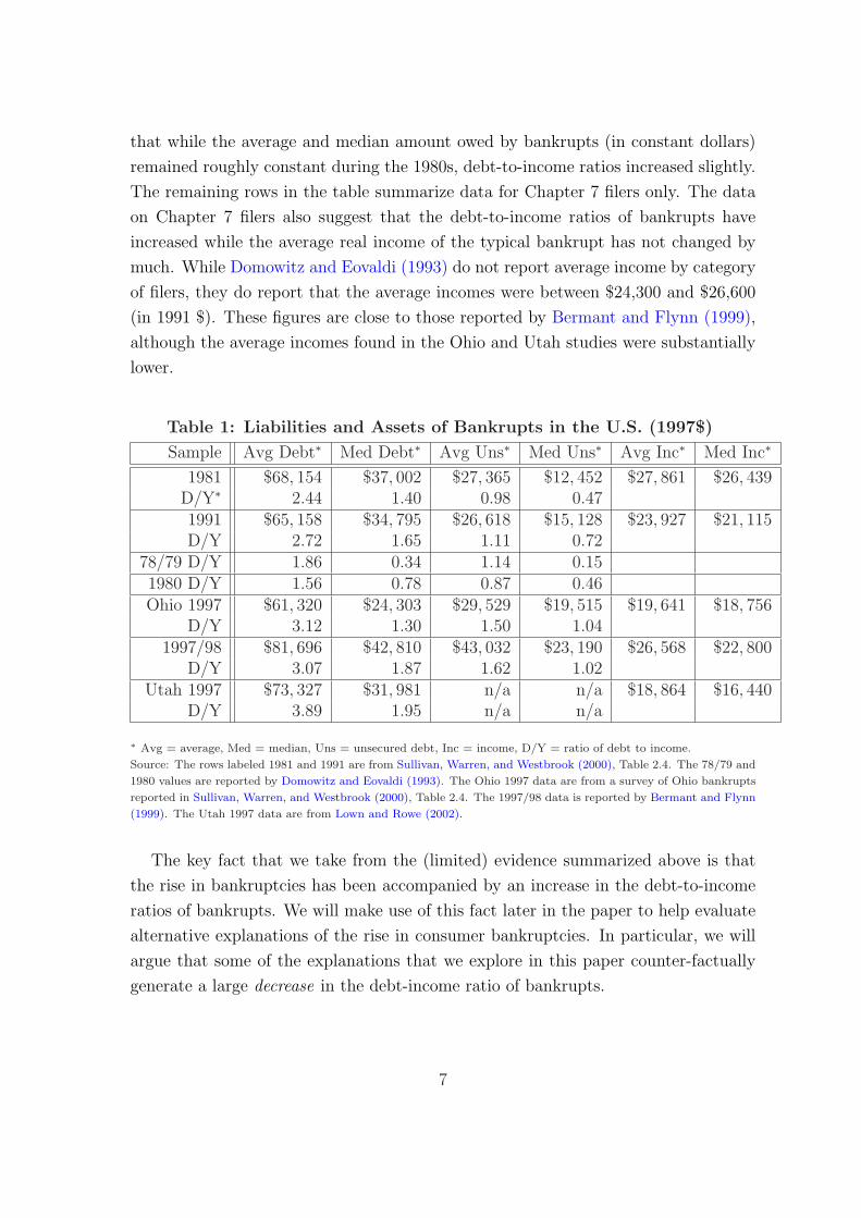
that while the average and median amount owed by bankrupts (in constant dollars)

remained roughly constant during the 1980s, debt-to-income ratios increased slightly.

The remaining rows in the table summarize data for Chapter 7 filers only. The data

on Chapter 7 filers also suggest that the debt-to-income ratios of bankrupts have

increased while the average real income of the typical bankrupt has not changed by

much. While Domowitz and Eovaldi (1993) do not report average income by category

of filers, they do report that the average incomes were between $24,300 and $26,600

(in 1991 $). These figures are close to those reported by Bermant and Flynn (1999),

although the average incomes found in the Ohio and Utah studies were substantially

lower.

Table 1: Liabilities and Assets of Bankrupts in the U.S. (1997$)

Sample Avg Debt∗ Med Debt∗ Avg Uns∗ Med Uns∗ Avg Inc∗ Med Inc∗

1981 $68, 154 $37, 002 $27, 365 $12, 452 $27, 861 $26, 439D/Y∗ 2.44 1.40 0.98 0.471991 $65, 158 $34, 795 $26, 618 $15, 128 $23, 927 $21, 115D/Y 2.72 1.65 1.11 0.72

78/79 D/Y 1.86 0.34 1.14 0.151980 D/Y 1.56 0.78 0.87 0.46Ohio 1997 $61, 320 $24, 303 $29, 529 $19, 515 $19, 641 $18, 756

D/Y 3.12 1.30 1.50 1.041997/98 $81, 696 $42, 810 $43, 032 $23, 190 $26, 568 $22, 800

D/Y 3.07 1.87 1.62 1.02Utah 1997 $73, 327 $31, 981 n/a n/a $18, 864 $16, 440

D/Y 3.89 1.95 n/a n/a

∗ Avg = average, Med = median, Uns = unsecured debt, Inc = income, D/Y = ratio of debt to income.

Source: The rows labeled 1981 and 1991 are from Sullivan, Warren, and Westbrook (2000), Table 2.4. The 78/79 and

1980 values are reported by Domowitz and Eovaldi (1993). The Ohio 1997 data are from a survey of Ohio bankrupts

reported in Sullivan, Warren, and Westbrook (2000), Table 2.4. The 1997/98 data is reported by Bermant and Flynn

(1999). The Utah 1997 data are from Lown and Rowe (2002).

The key fact that we take from the (limited) evidence summarized above is that

the rise in bankruptcies has been accompanied by an increase in the debt-to-income

ratios of bankrupts. We will make use of this fact later in the paper to help evaluate

alternative explanations of the rise in consumer bankruptcies. In particular, we will

argue that some of the explanations that we explore in this paper counter-factually

generate a large decrease in the debt-income ratio of bankrupts.

7

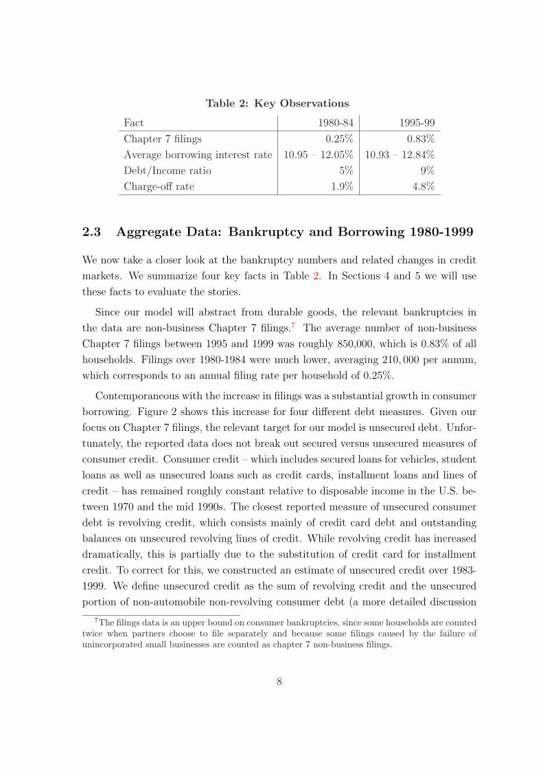
Table 2: Key Observations

Fact 1980-84 1995-99

Chapter 7 filings 0.25% 0.83%

Average borrowing interest rate 10.95 – 12.05% 10.93 – 12.84%

Debt/Income ratio 5% 9%

Charge-off rate 1.9% 4.8%

2.3 Aggregate Data: Bankruptcy and Borrowing 1980-1999

We now take a closer look at the bankruptcy numbers and related changes in credit

markets. We summarize four key facts in Table 2. In Sections 4 and 5 we will use

these facts to evaluate the stories.

Since our model will abstract from durable goods, the relevant bankruptcies in

the data are non-business Chapter 7 filings.7 The average number of non-business

Chapter 7 filings between 1995 and 1999 was roughly 850,000, which is 0.83% of all

households. Filings over 1980-1984 were much lower, averaging 210, 000 per annum,

which corresponds to an annual filing rate per household of 0.25%.

Contemporaneous with the increase in filings was a substantial growth in consumer

borrowing. Figure 2 shows this increase for four different debt measures. Given our

focus on Chapter 7 filings, the relevant target for our model is unsecured debt. Unfor-

tunately, the reported data does not break out secured versus unsecured measures of

consumer credit. Consumer credit – which includes secured loans for vehicles, student

loans as well as unsecured loans such as credit cards, installment loans and lines of

credit – has remained roughly constant relative to disposable income in the U.S. be-

tween 1970 and the mid 1990s. The closest reported measure of unsecured consumer

debt is revolving credit, which consists mainly of credit card debt and outstanding

balances on unsecured revolving lines of credit. While revolving credit has increased

dramatically, this is partially due to the substitution of credit card for installment

credit. To correct for this, we constructed an estimate of unsecured credit over 1983-

1999. We define unsecured credit as the sum of revolving credit and the unsecured

portion of non-automobile non-revolving consumer debt (a more detailed discussion

7The filings data is an upper bound on consumer bankruptcies, since some households are countedtwice when partners choose to file separately and because some filings caused by the failure ofunincorporated small businesses are counted as chapter 7 non-business filings.

8

is in Appendix A). The estimates are plotted in Figure 3 as a percentage of personal

disposable income, along with revolving credit. While our calculations suggest that

the rise in revolving debt significantly overstates the increase in unsecured debt, they

also imply a substantial increase between 1983 and 1999 in the unsecured debt to

income ratio. This gives a debt-income ratio of roughly 9% for the late 1990s and 5%

for the early 1980s.

The Federal Reserve reports two interest rates on unsecured loans for the time

periods we examine – the average (nominal) interest rate for two-year personal loans

and the average interest rate on credit cards. We compute the real rate of interest

using the one-year ahead CPI inflation rate and then compute the average for each

of the two periods, 1981-1985 and 1996-2000. This calculation implies an average

real cost of unsecured consumer borrowing between 11% and 13% (about 11.0% for

personal loans and 13.0% for credit cards). Somewhat surprisingly, there is little

change in these interest rates over time.8

The small change in real borrowing interest rates is even more surprising given

the increased rate of non-repayments on consumer loans. One common measure of

non-payment is charge-off rates, which measure the value of loans written off (net

of recoveries) and charged against loss reserves as a percentage of average loans.9

Unfortunately, the charge-off rate series constructed by the Board of Governors begins

in 1985. To extend this series backwards, we splice this series with a series reported

by Ausubel (1991).10 The average one-year ahead charge-offs on credit cards have

increased from about 1.9% to 4.8% between the 1981-85 and 1996-2000 periods. As

Figure 4 illustrates, charge-offs move in parallel with the bankruptcy rate.

3 Basic Environment for Evaluating the Stories

In this section, we briefly outline the model used to evaluate the stories, and describe

our benchmark parametrization which serves as a starting point for the numerical

experiments.

8One might expect an increase in the real rate given the high inflation rates during the late 1970sand early 1980s. However, nominal interest rates on personal loans fell during this time (from 17%to 13.7%), while average inflation declined from 5.5% in 1981-85 to 2.5% in 1996-2000.

9See Furletti (2003b) for an overview of data sources and measurement methodology of charge-offs. While roughly 40% of credit card charge-offs are due to bankruptcies, the rest is mandatorycharge-offs in response to delinquent loans, many of which ultimately end up in bankruptcy.

10While the level of the Ausubel series is slightly below that of the Board series, the two seriesmove together for the years they overlap.

9

3.1 The Model

We extend the “Fresh Start” model of consumer bankruptcy of Livshits, MacGee,

and Tertilt (2007) by allowing for three additional costs of bankruptcy (a utility cost,

a burning cost and a fixed cost of filing) as well as an interest rate ceiling. These

extensions allow us to evaluate several channels via which changes in the credit market

environment could potentially have caused the rise in bankruptcies.

The model economy is populated by overlapping generations of J period lived

households. Each generation is comprised of measure 1 of households facing idiosyn-

cratic uncertainty. There is no aggregate uncertainty. Markets are incomplete and

agents can borrow using non-contingent person-specific one-period bonds and save at

an exogenously given interest rate. Households have the option to declare bankruptcy.

Households

Household maximize expected discounted life-time utility from consumption:

E

J∑j=1

βj−1u

(cj

nj

)(3.1)

where β is the discount factor, cj is household consumption and nj is the size of a

household of age j in equivalence scale units.

The labor income of a household i of age j is the product of an age-dependent

labor endowment and productivity shocks:

yij = ejz

ijη

ij, (3.2)

where ej is the deterministic endowment of efficiency units of labor, zij is a persistent

shock to the household’s earnings, and ηij a transitory shock.

Households face a second type of uncertainty: They may be hit with an idiosyn-

cratic expense shock κ ≥ 0, κ ∈ K, where K is a finite set of possible expense shocks.

The probability of shock κi is denoted πi. An expense shock directly changes the

net asset position of a household. Expense shocks are independently and identically

distributed, and are independent of income shocks.

A household can file for bankruptcy. We model bankruptcy so as to capture the

most salient features of Chapter 7 consumer bankruptcy in the U.S. As in Chapter

7, upon filing all debts are discharged, and the household enters the following period

with a balance of zero (unless hit by an expense shock that period). Filers also face

10

several types of “punishment” which proxy for specific features of Chapter 7. First,

bankrupts cannot save or borrow during the default period because all assets are

seized during a Chapter 7 bankruptcy. Second, bankruptcy cannot be declared two

periods in a row.11 Third, the US bankruptcy code specifies that borrowers must act

in “good faith” so that borrowing and immediately filing for bankruptcy is sometimes

denied. To capture the requirement that borrowers make a good faith effort to repay

their debt, we force bankrupt households to repay a fraction γ of their earnings during

the period in which they file.12

In our experiments involving potential credit market changes we consider three

other potential costs of bankruptcy. The first is a utility cost of filing, χ. This

“stigma” may reflect real or psychic (“shame”) costs of bankruptcy. The second is

the “burning” of a fraction λ of filers’ consumption during the bankruptcy period.

This is meant to capture the increased cost of consumption (finding an apartment,

limited access to credit cards for purchases, etc.) after bankruptcy. Finally, we also

allow for a fixed cost φ of bankruptcy, which captures the legal costs of filing.

The timing is as follows. At the beginning of the period, each household realizes

its productivity and expense shocks. If the household receives an expense shock,

then the debt of the household is increased (or savings decreased) by the amount

of the shock. The household then decides whether to file for bankruptcy or not. If

bankruptcy is declared, creditors garnishee labor income and the consumer is allowed

to spend the remaining income. Filers are not allowed to save or borrow, thus, they

consume all earnings net of debt-recovery γ (and “burning”). Households who do not

declare bankruptcy decide on their asset holdings for the following period and their

current consumption.

Financial Intermediaries

Financial markets are perfectly competitive. Intermediaries accept deposits from

savers and make loans to borrowers. The risk-free savings rate rs is given exogenously.

Loans take the form of one period non-contingent bond contracts. However, the

11In our numerical experiments, each period lasts for 3 years, so this captures the fact that underChapter 7 households have to wait at least 6 years before filing again.

12Prior to 1984, courts had the implicit right to dismiss a case based on “bad faith” behaviourby the debtor. The Bankruptcy Amendments and Federal Judgeship act of 1984 and the 1986amendments to section 707(b) of the Code formalized this by explicitly allowing bankruptcy trusteesto make a motion for dismissal for substantial abuse. While the interpretation of “substantial abuse”has varied across courts, the ability to repay a significant fraction of one’s debt has often played alarge role in courts’ decisions to dismiss debtors’ bankruptcy petitions (see Cain (1997) and Wells,Kurtz, and Calhoun (1991)).

11

bankruptcy option introduces a partial contingency by allowing filers to discharge

their debts. The face value of a loan to be repaid next period is denoted by d′.

Savings are denoted by d′ < 0. Intermediaries incur a proportional transaction cost

of making loans, τ .

Intermediaries have complete information about borrowers: They observe the total

level of borrowing d′, the current persistent productivity shock z, and the borrower’s

age j.This allows intermediaries to accurately forecast the default probability of a

borrower, θ(d′, z, j), and price the loan accordingly.

Equilibrium

In equilibrium, perfect competition and complete information imply that intermedi-

aries make zero expected profit on each loan and that cross subsidization of interest

rates across different types of borrowers does not occur. Therefore the individual

bond price is determined by the default probability of the issuer and the risk-free

bond price. Without debt-recovery, without usury law and with full discharge of

debt, the zero profit condition is qb(d′, z, j) = (1 − θ(d′, z, j))qb, where qb(= 1

1+rs+τ

)

is the price of a bond with zero default probability.

For positive levels of debt-recovery, this formula needs to be adjusted. The unre-

stricted bond price under debt recovery is

qub(d′, z, j) = (1− θ(d′, z, j))qb + θ(d′, z, j)E(γy

d′ + κ′)qb (3.3)

where E( γyd′+κ′ ) is the expected rate of recovery, assuming that when a household de-

faults, the amount recovered is allocated proportionately to expense debt and personal

loans.

Lastly, taking into account the interest rate ceiling r, the equilibrium bond price is

qb(d′, z, j) =

{qub(d′, z, j) if qub(d′, z, j) > 1

1+r

0 otherwise(3.4)

Households take the bond price schedule as given when making decisions. The

problem of a household is defined recursively using three distinct value functions.

V is the value of a “normal period,” while V is the value of declaring bankruptcy.

Although bankruptcy cannot be declared two periods in a row, a household may

not be able to repay the realized value of an expense shock in a period following

bankruptcy. In this case, the household’s current income is garnisheed and its debt

is rolled over at a fixed interest rate rr. The value of this state of the world is W .

12

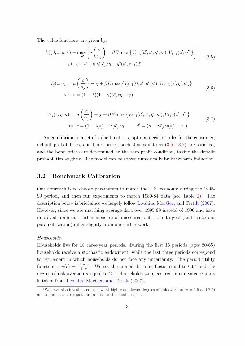
The value functions are given by:

Vj(d, z, η, κ) = maxc,d′

[u

(c

nj

)+ βE max

{Vj+1(d

′, z′, η′, κ′), Vj+1(z′, η′)

}]

s.t. c + d + κ 6 ejzη + qb(d′, z, j)d′(3.5)

Vj(z, η) = u

(c

nj

)− χ + βE max {Vj+1(0, z

′, η′, κ′),Wj+1(z′, η′, κ′)}

s.t. c = (1− λ)(1− γ)(ejzη − φ)

(3.6)

Wj(z, η, κ) = u

(c

nj

)− χ + βE max

{Vj+1(d

′, z′, η′, κ′), Vj+1(z′, η′)

}

s.t. c = (1− λ)(1− γ)ejzη, d′ = (κ− γejzη)(1 + rr)

(3.7)

An equilibrium is a set of value functions, optimal decision rules for the consumer,

default probabilities, and bond prices, such that equations (3.5)-(3.7) are satisfied,

and the bond prices are determined by the zero profit condition, taking the default

probabilities as given. The model can be solved numerically by backwards induction.

3.2 Benchmark Calibration

Our approach is to choose parameters to match the U.S. economy during the 1995-

99 period, and then run experiments to match 1980-84 data (see Table 2). The

description below is brief since we largely follow Livshits, MacGee, and Tertilt (2007).

However, since we are matching average data over 1995-99 instead of 1996 and have

improved upon our earlier measure of unsecured debt, our targets (and hence our

parametrization) differ slightly from our earlier work.

Households

Households live for 18 three-year periods. During the first 15 periods (ages 20-65)

households receive a stochastic endowment, while the last three periods correspond

to retirement in which households do not face any uncertainty. The period utility

function is u(c) = c1−σ−11−σ

. We set the annual discount factor equal to 0.94 and the

degree of risk aversion σ equal to 2.13 Household size measured in equivalence units

is taken from Livshits, MacGee, and Tertilt (2007).

13We have also investigated somewhat higher and lower degrees of risk aversion (σ = 1.5 and 2.5)and found that our results are robust to this modification.

13

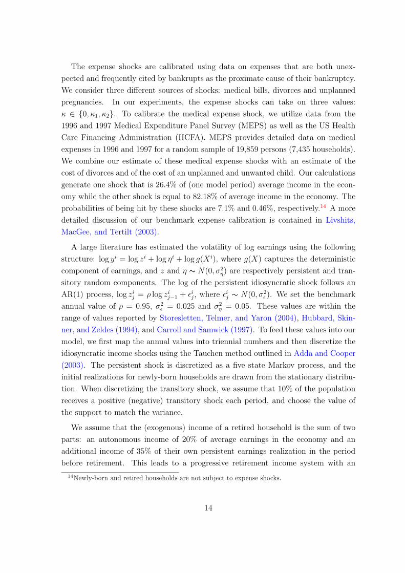
The expense shocks are calibrated using data on expenses that are both unex-

pected and frequently cited by bankrupts as the proximate cause of their bankruptcy.

We consider three different sources of shocks: medical bills, divorces and unplanned

pregnancies. In our experiments, the expense shocks can take on three values:

κ ∈ {0, κ1, κ2}. To calibrate the medical expense shock, we utilize data from the

1996 and 1997 Medical Expenditure Panel Survey (MEPS) as well as the US Health

Care Financing Administration (HCFA). MEPS provides detailed data on medical

expenses in 1996 and 1997 for a random sample of 19,859 persons (7,435 households).

We combine our estimate of these medical expense shocks with an estimate of the

cost of divorces and of the cost of an unplanned and unwanted child. Our calculations

generate one shock that is 26.4% of (one model period) average income in the econ-

omy while the other shock is equal to 82.18% of average income in the economy. The

probabilities of being hit by these shocks are 7.1% and 0.46%, respectively.14 A more

detailed discussion of our benchmark expense calibration is contained in Livshits,

MacGee, and Tertilt (2003).

A large literature has estimated the volatility of log earnings using the following

structure: log yi = log zi + log ηi + log g(X i), where g(X) captures the deterministic

component of earnings, and z and η ∼ N(0, σ2η) are respectively persistent and tran-

sitory random components. The log of the persistent idiosyncratic shock follows an

AR(1) process, log zij = ρ log zi

j−1 + εij, where εi

j ∼ N(0, σ2ε ). We set the benchmark

annual value of ρ = 0.95, σ2ε = 0.025 and σ2

η = 0.05. These values are within the

range of values reported by Storesletten, Telmer, and Yaron (2004), Hubbard, Skin-

ner, and Zeldes (1994), and Carroll and Samwick (1997). To feed these values into our

model, we first map the annual values into triennial numbers and then discretize the

idiosyncratic income shocks using the Tauchen method outlined in Adda and Cooper

(2003). The persistent shock is discretized as a five state Markov process, and the

initial realizations for newly-born households are drawn from the stationary distribu-

tion. When discretizing the transitory shock, we assume that 10% of the population

receives a positive (negative) transitory shock each period, and choose the value of

the support to match the variance.

We assume that the (exogenous) income of a retired household is the sum of two

parts: an autonomous income of 20% of average earnings in the economy and an

additional income of 35% of their own persistent earnings realization in the period

before retirement. This leads to a progressive retirement income system with an

14Newly-born and retired households are not subject to expense shocks.

14

average replacement rate of 55%, which is within the range of numbers reported in

Butrica, Iams, and Smith (2004). Note that total retirement income is higher as

households also have private savings.

Financial Market Parameters

The savings interest rate is set equal to 3.44%, as in Gourinchas and Parker (2002).

The rollover interest rate rr is set to 20% annual. The cost of filing for bankruptcy

parameters — the utility cost χ, the fixed cost φ, and the fraction of consumption

lost λ — are set to 0 in the benchmark economy.

The three remaining parameters — the debt recovery rate γ, transaction cost τ , and

the interest rate ceiling r — are chosen to match the facts from Table 2 for 1995-1999.

This leads to a γ of 0.319.15 The transactions cost of making loans is 2.56% annually.

Together with the risk-free savings interest rate of 3.44%, this implies an annual risk-

free lending rate of 6%. Finally, the interest rate ceiling is set to a (high) value of

75% annually. While this value exceeds the current official interest rate ceilings, there

are many ways to (partially) get around the official legal ceilings.16 This ceiling is

not binding for almost all of the consumers in our experiments. However, having

no ceiling can sometimes lead to a (very) small number of people borrowing large

amounts at very high interest rates (with little intention of repaying them), which

leads to artificially high average interest rates.

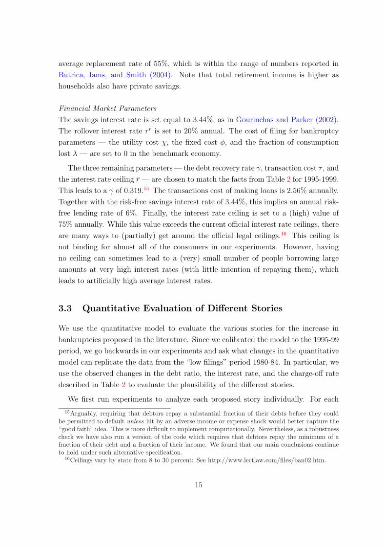
3.3 Quantitative Evaluation of Different Stories

We use the quantitative model to evaluate the various stories for the increase in

bankruptcies proposed in the literature. Since we calibrated the model to the 1995-99

period, we go backwards in our experiments and ask what changes in the quantitative

model can replicate the data from the “low filings” period 1980-84. In particular, we

use the observed changes in the debt ratio, the interest rate, and the charge-off rate

described in Table 2 to evaluate the plausibility of the different stories.

We first run experiments to analyze each proposed story individually. For each

15Arguably, requiring that debtors repay a substantial fraction of their debts before they couldbe permitted to default unless hit by an adverse income or expense shock would better capture the“good faith” idea. This is more difficult to implement computationally. Nevertheless, as a robustnesscheck we have also run a version of the code which requires that debtors repay the minimum of afraction of their debt and a fraction of their income. We found that our main conclusions continueto hold under such alternative specification.

16Ceilings vary by state from 8 to 30 percent: See http://www.lectlaw.com/files/ban02.htm.

15

story we ask whether the implied amount of borrowing, the interest rate and the

charge-off rate are consistent with the data for the low filing period (Table 2). The

next section focuses on uncertainty based stories, while section 5 examines credit

market based channels. In Section 6, we build on these experiments and decompose

the relative importance of a combination of uncertainty and credit market based

stories for the rise in consumer bankruptcies.

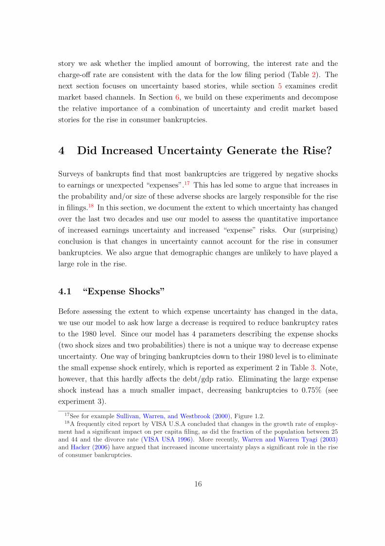
4 Did Increased Uncertainty Generate the Rise?

Surveys of bankrupts find that most bankruptcies are triggered by negative shocks

to earnings or unexpected “expenses”.17 This has led some to argue that increases in

the probability and/or size of these adverse shocks are largely responsible for the rise

in filings.18 In this section, we document the extent to which uncertainty has changed

over the last two decades and use our model to assess the quantitative importance

of increased earnings uncertainty and increased “expense” risks. Our (surprising)

conclusion is that changes in uncertainty cannot account for the rise in consumer

bankruptcies. We also argue that demographic changes are unlikely to have played a

large role in the rise.

4.1 “Expense Shocks”

Before assessing the extent to which expense uncertainty has changed in the data,

we use our model to ask how large a decrease is required to reduce bankruptcy rates

to the 1980 level. Since our model has 4 parameters describing the expense shocks

(two shock sizes and two probabilities) there is not a unique way to decrease expense

uncertainty. One way of bringing bankruptcies down to their 1980 level is to eliminate

the small expense shock entirely, which is reported as experiment 2 in Table 3. Note,

however, that this hardly affects the debt/gdp ratio. Eliminating the large expense

shock instead has a much smaller impact, decreasing bankruptcies to 0.75% (see

experiment 3).

17See for example Sullivan, Warren, and Westbrook (2000), Figure 1.2.18A frequently cited report by VISA U.S.A concluded that changes in the growth rate of employ-

ment had a significant impact on per capita filing, as did the fraction of the population between 25and 44 and the divorce rate (VISA USA 1996). More recently, Warren and Warren Tyagi (2003)and Hacker (2006) have argued that increased income uncertainty plays a significant role in the riseof consumer bankruptcies.

16

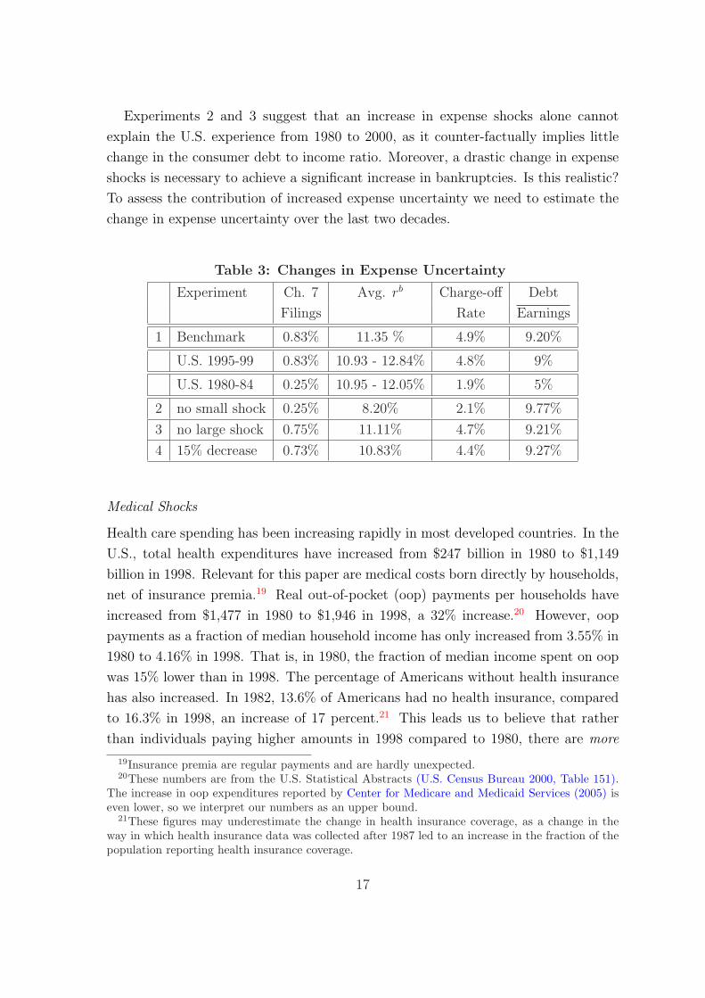
Experiments 2 and 3 suggest that an increase in expense shocks alone cannot

explain the U.S. experience from 1980 to 2000, as it counter-factually implies little

change in the consumer debt to income ratio. Moreover, a drastic change in expense

shocks is necessary to achieve a significant increase in bankruptcies. Is this realistic?

To assess the contribution of increased expense uncertainty we need to estimate the

change in expense uncertainty over the last two decades.

Table 3: Changes in Expense Uncertainty

Experiment Ch. 7 Avg. rb Charge-off Debt

Filings Rate Earnings

1 Benchmark 0.83% 11.35 % 4.9% 9.20%

U.S. 1995-99 0.83% 10.93 - 12.84% 4.8% 9%

U.S. 1980-84 0.25% 10.95 - 12.05% 1.9% 5%

2 no small shock 0.25% 8.20% 2.1% 9.77%

3 no large shock 0.75% 11.11% 4.7% 9.21%

4 15% decrease 0.73% 10.83% 4.4% 9.27%

Medical Shocks

Health care spending has been increasing rapidly in most developed countries. In the

U.S., total health expenditures have increased from $247 billion in 1980 to $1,149

billion in 1998. Relevant for this paper are medical costs born directly by households,

net of insurance premia.19 Real out-of-pocket (oop) payments per households have

increased from $1,477 in 1980 to $1,946 in 1998, a 32% increase.20 However, oop

payments as a fraction of median household income has only increased from 3.55% in

1980 to 4.16% in 1998. That is, in 1980, the fraction of median income spent on oop

was 15% lower than in 1998. The percentage of Americans without health insurance

has also increased. In 1982, 13.6% of Americans had no health insurance, compared

to 16.3% in 1998, an increase of 17 percent.21 This leads us to believe that rather

than individuals paying higher amounts in 1998 compared to 1980, there are more

19Insurance premia are regular payments and are hardly unexpected.20These numbers are from the U.S. Statistical Abstracts (U.S. Census Bureau 2000, Table 151).

The increase in oop expenditures reported by Center for Medicare and Medicaid Services (2005) iseven lower, so we interpret our numbers as an upper bound.

21These figures may underestimate the change in health insurance coverage, as a change in theway in which health insurance data was collected after 1987 led to an increase in the fraction of thepopulation reporting health insurance coverage.

17

people with large out-of-pocket expenditures. Furthermore, (based on unreported

experiments), the bankruptcy filing rate in the model is more sensitive to changes

in the probability of the shock than its size. Thus, decreasing the expense shock

probabilities by 15% should yield an upper bound on how much of the change in

the filing rate could come through this channel.22 Based on experiment 4 in Table

3, we conclude that medical shocks can account for less than 20 percent of the rise

in bankruptcies, and cannot account for the increase in consumer debt. Given that

defaults do not change much, it is not surprising that this experiment also cannot

replicate the large increase in charge-offs.

The comparison with Canada casts further doubt on changes in medical uncertainty

being the main driving force behind the rise in filings. Canada is a country with

universal health care coverage. Hence, catastrophic medical expenses are unlikely

to be the main cause of bankruptcies in Canada, which is consistent with the lower

level of bankruptcies relative to the U.S. However, Canada experienced a very similar

increase in bankruptcies (see Figure 1), which suggests that a factor common to both

countries is primarily responsible. This leads us to conclude that changes in the cost

and extent of insurance against catastrophic medical events are not the primary factor

driving the rise in bankruptcies.

Family Shocks

Sullivan, Warren, and Westbrook (2000) emphasize the importance of unexpected

family-related events for bankruptcy. In their 1991 bankruptcy survey, 22% of re-

spondents cited family factors as a main cause of their bankruptcy. The obvious two

causes for sudden family related expenses are divorces and unplanned pregnancies.

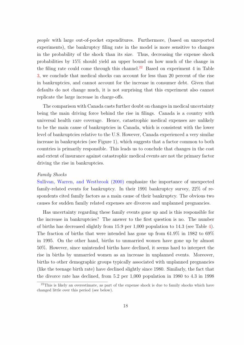
Has uncertainty regarding these family events gone up and is this responsible for

the increase in bankruptcies? The answer to the first question is no. The number

of births has decreased slightly from 15.9 per 1,000 population to 14.3 (see Table 4).

The fraction of births that were intended has gone up from 61.9% in 1982 to 69%

in 1995. On the other hand, births to unmarried women have gone up by almost

50%. However, since unintended births have declined, it seems hard to interpret the

rise in births by unmarried women as an increase in unplanned events. Moreover,

births to other demographic groups typically associated with unplanned pregnancies

(like the teenage birth rate) have declined slightly since 1980. Similarly, the fact that

the divorce rate has declined, from 5.2 per 1,000 population in 1980 to 4.3 in 1998

22This is likely an overestimate, as part of the expense shock is due to family shocks which havechanged little over this period (see below).

18

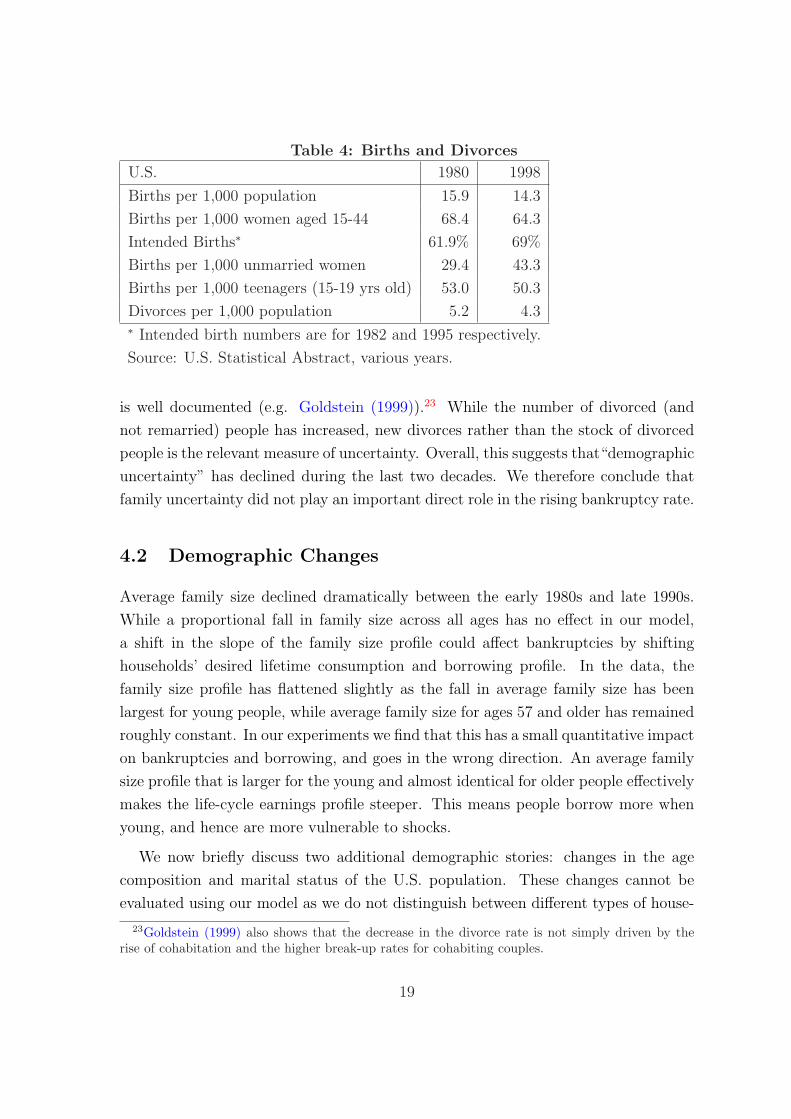
Table 4: Births and Divorces

U.S. 1980 1998

Births per 1,000 population 15.9 14.3

Births per 1,000 women aged 15-44 68.4 64.3

Intended Births∗ 61.9% 69%

Births per 1,000 unmarried women 29.4 43.3

Births per 1,000 teenagers (15-19 yrs old) 53.0 50.3

Divorces per 1,000 population 5.2 4.3∗ Intended birth numbers are for 1982 and 1995 respectively.

Source: U.S. Statistical Abstract, various years.

is well documented (e.g. Goldstein (1999)).23 While the number of divorced (and

not remarried) people has increased, new divorces rather than the stock of divorced

people is the relevant measure of uncertainty. Overall, this suggests that“demographic

uncertainty” has declined during the last two decades. We therefore conclude that

family uncertainty did not play an important direct role in the rising bankruptcy rate.

4.2 Demographic Changes

Average family size declined dramatically between the early 1980s and late 1990s.

While a proportional fall in family size across all ages has no effect in our model,

a shift in the slope of the family size profile could affect bankruptcies by shifting

households’ desired lifetime consumption and borrowing profile. In the data, the

family size profile has flattened slightly as the fall in average family size has been

largest for young people, while average family size for ages 57 and older has remained

roughly constant. In our experiments we find that this has a small quantitative impact

on bankruptcies and borrowing, and goes in the wrong direction. An average family

size profile that is larger for the young and almost identical for older people effectively

makes the life-cycle earnings profile steeper. This means people borrow more when

young, and hence are more vulnerable to shocks.

We now briefly discuss two additional demographic stories: changes in the age

composition and marital status of the U.S. population. These changes cannot be

evaluated using our model as we do not distinguish between different types of house-

23Goldstein (1999) also shows that the decrease in the divorce rate is not simply driven by therise of cohabitation and the higher break-up rates for cohabiting couples.

19

holds (single vs. married) nor do we allow changes in cohort size. However, some

back-of-the envelope calculations suggest that these are not important contributors

to the increase in consumer bankruptcies.

Table 5 shows that bankruptcy filing rates are a hump-shaped function of age.

Sullivan, Warren, and Westbrook (2000) argue that the aging of the baby-boomers

through the high risk age groups accounts for 18% of the increase in bankruptcies be-

tween 1981 and 1991. We redid their analysis and constructed the implied bankruptcy

rates between 1980 and 2001, holding age specific filings rates constant at their 1991

and 2001 levels respectively. Figure 5 contrasts the constructed filings rates per 1,000

households with the actual numbers. The graph shows that changes in the age struc-

ture alone had no impact on the aggregate filings rates. The discrepancy between

our results and Sullivan, Warren, and Westbrook (2000) is due to the distinction be-

tween an increase in total filings and filings per 1,000 population. The total number

of bankruptcies increases because the U.S. population grew by 17% between 1981 and

1991, but this is unrelated to changes in age composition.

Table 5: Filings per 1,000 adults by age in the U.S.

Age < 25 25-34 35-44 45-54 55-64 65 + avg.

1991 3.4 6.8 6.5 5.2 2.7 0.6 4.62001 3.8 8.9 9.8 8.1 4.1 2.0 6.6

Source: Sullivan, Thorne, and Warren (2001), Table 1 (primary petitioners only).24

The second change is the dramatic rise in the share of bankruptcies filed by

women.25 The percentage of bankruptcies filed by women has increased from less

than 15% in 1967 to almost 40% in 1999. However, filing rates by gender are hard to

interpret. Married couples can choose to file jointly, separately, or only one spouse

could file. Therefore, the link between increases in the filing rate of women and the

increased number of single women is not obvious. Filing rates by marital status are

more meaningful in this context. Unfortunately, marital status data is not routinely

collected by bankruptcy courts. Some evidence comes from Sullivan, Warren, and

Westbrook (2000), who asked about marital status in their 1991 survey of bankrupts.

Table 6 shows that a higher fraction of singles and especially of divorced people file for

bankruptcy compared to married people. Since the fraction of singles and divorcees

24These filing rates differ slightly from those used in the paper as they include Chapter 13 filings.25See Sullivan and Warren (1999) and Pollak (1997).

20

has increased substantially during the last two decades, it seems plausible that these

demographic changes are in part responsible for the trend in bankruptcies.

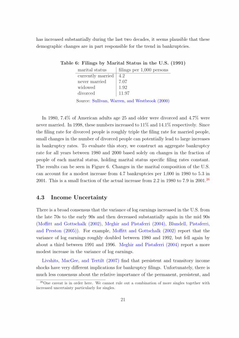
Table 6: Filings by Marital Status in the U.S. (1991)

marital status filings per 1,000 personscurrently married 4.2never married 7.07widowed 1.92divorced 11.97

Source: Sullivan, Warren, and Westbrook (2000)

In 1980, 7.4% of American adults age 25 and older were divorced and 4.7% were

never married. In 1998, these numbers increased to 11% and 14.1% respectively. Since

the filing rate for divorced people is roughly triple the filing rate for married people,

small changes in the number of divorced people can potentially lead to large increases

in bankruptcy rates. To evaluate this story, we construct an aggregate bankruptcy

rate for all years between 1980 and 2000 based solely on changes in the fraction of

people of each marital status, holding marital status specific filing rates constant.

The results can be seen in Figure 6. Changes in the marital composition of the U.S.

can account for a modest increase from 4.7 bankruptcies per 1,000 in 1980 to 5.3 in

2001. This is a small fraction of the actual increase from 2.2 in 1980 to 7.9 in 2001.26

4.3 Income Uncertainty

There is a broad consensus that the variance of log earnings increased in the U.S. from

the late 70s to the early 90s and then decreased substantially again in the mid 90s

(Moffitt and Gottschalk (2002), Meghir and Pistaferri (2004), Blundell, Pistaferri,

and Preston (2005)). For example, Moffitt and Gottschalk (2002) report that the

variance of log earnings roughly doubled between 1980 and 1992, but fell again by

about a third between 1991 and 1996. Meghir and Pistaferri (2004) report a more

modest increase in the variance of log earnings.

Livshits, MacGee, and Tertilt (2007) find that persistent and transitory income

shocks have very different implications for bankruptcy filings. Unfortunately, there is

much less consensus about the relative importance of the permanent, persistent, and

26One caveat is in order here. We cannot rule out a combination of more singles together withincreased uncertainty particularly for singles.

21

transitory components in accounting for the increased variance of log earnings. Moffitt

and Gottschalk (2002) argue that the variance of the permanent shock increased by

roughly 50 percent between 1980 and 1996, while the variance of transitory shocks

doubled from 1980 to 1985, levelled off until about 1992, after which it declined

sharply by about 50 percent. Meghir and Pistaferri (2004), on the other hand, find a

sharp increase in the variance of the permanent shock between the mid 70s and 1985,

after which it fell and by 1987 was back to its 1978 level. Blundell, Pistaferri, and

Preston (2005) find that the variance of the permanent shock doubled between 1980

and 1985, then declined, and that the transitory variance increased by roughly 50

percent from 1980 to 1987, followed by a fall. Finally, Heathcoate, Storesletten, and

Violante (2004) analyze log hourly wages, rather than earnings, and decompose them

into permanent, persistent, and transitory components for the years 1967 to 1996.

Their estimates imply that the variance of the transitory shock increased by 25 to

30 percent (depending on which years one uses), while the variance of the persistent

shock remained constant or decreased slightly.

In the experiments we run, we take the most generous estimates of the increase in

persistent and transitory income uncertainty to get an upper bound on the impact of

income uncertainty. We investigate an increase in the variance of the transitory shock

in excess of 30%. Since we do not have permanent shocks in the model, we increase

the variance of persistent shocks to represent possible increases in both persistent and

permanent uncertainty in the data. To obtain an upper bound on the impact of these

shocks, we increase the variance of the persistent shock by 150%. We then shut down

the income shocks completely to show that income uncertainty cannot account for a

large part of the rise in filings. The results are reported in Table 7.

Experiment 1 shows that lowering the variance of the transitory income shocks

by 25% (i.e., a 33% increase over the two decades) has almost no effect – in fact,

it slightly increases filings. Experiment 2 illustrates that even shutting down the

transitory income shock completely does not change the number of filings. This

suggests that a change in transitory income uncertainty cannot be a driving force

behind the increase in bankruptcy filings.

In experiment 3, we lower the variance of the persistent shocks by 60% (corre-

sponding to a 2.5-fold increase over the two decades). This decline in the variance

decreases the filings to 0.80%, while driving the unsecured debt up to almost 15% of

earnings. Experiment 4 shows that lowering the variance of the persistent shocks by

another 60% only reduces filings to 0.78%. Finally, shutting down persistent shocks

22

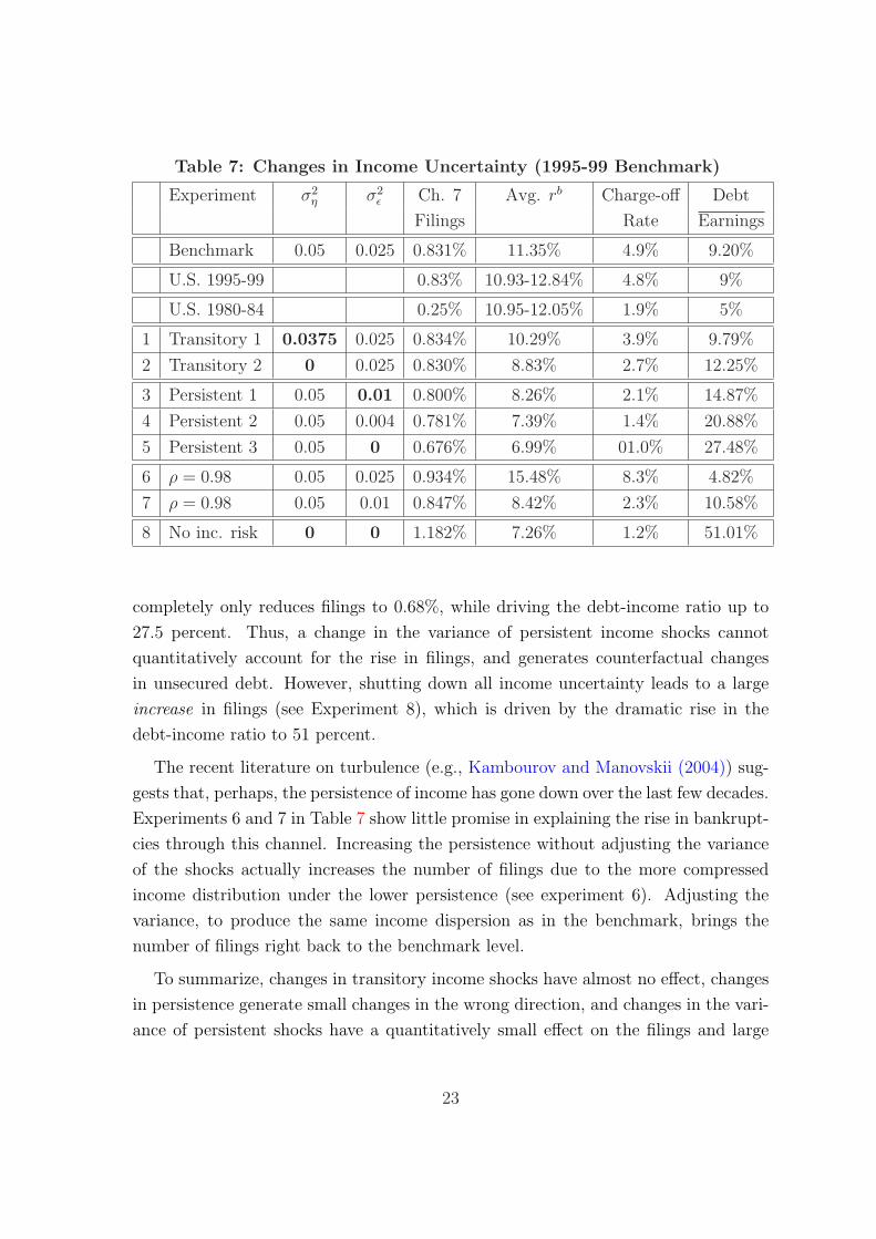
Table 7: Changes in Income Uncertainty (1995-99 Benchmark)

Experiment σ2η σ2

ε Ch. 7 Avg. rb Charge-off Debt

Filings Rate Earnings

Benchmark 0.05 0.025 0.831% 11.35% 4.9% 9.20%

U.S. 1995-99 0.83% 10.93-12.84% 4.8% 9%

U.S. 1980-84 0.25% 10.95-12.05% 1.9% 5%

1 Transitory 1 0.0375 0.025 0.834% 10.29% 3.9% 9.79%

2 Transitory 2 0 0.025 0.830% 8.83% 2.7% 12.25%

3 Persistent 1 0.05 0.01 0.800% 8.26% 2.1% 14.87%

4 Persistent 2 0.05 0.004 0.781% 7.39% 1.4% 20.88%

5 Persistent 3 0.05 0 0.676% 6.99% 01.0% 27.48%

6 ρ = 0.98 0.05 0.025 0.934% 15.48% 8.3% 4.82%

7 ρ = 0.98 0.05 0.01 0.847% 8.42% 2.3% 10.58%

8 No inc. risk 0 0 1.182% 7.26% 1.2% 51.01%

completely only reduces filings to 0.68%, while driving the debt-income ratio up to

27.5 percent. Thus, a change in the variance of persistent income shocks cannot

quantitatively account for the rise in filings, and generates counterfactual changes

in unsecured debt. However, shutting down all income uncertainty leads to a large

increase in filings (see Experiment 8), which is driven by the dramatic rise in the

debt-income ratio to 51 percent.

The recent literature on turbulence (e.g., Kambourov and Manovskii (2004)) sug-

gests that, perhaps, the persistence of income has gone down over the last few decades.

Experiments 6 and 7 in Table 7 show little promise in explaining the rise in bankrupt-

cies through this channel. Increasing the persistence without adjusting the variance

of the shocks actually increases the number of filings due to the more compressed

income distribution under the lower persistence (see experiment 6). Adjusting the

variance, to produce the same income dispersion as in the benchmark, brings the

number of filings right back to the benchmark level.

To summarize, changes in transitory income shocks have almost no effect, changes

in persistence generate small changes in the wrong direction, and changes in the vari-

ance of persistent shocks have a quantitatively small effect on the filings and large

23

effect (in the wrong direction) on debt. The inability of realistic changes in transi-

tory income shocks to generate large changes in filings is not surprising. Households

tend to smooth transitory income shocks over time through borrowing and saving

rather than by declaring bankruptcy. Since borrowing and saving are not as use-

ful in smoothing persistent income shocks, they can in principle have a large effect

on filings. However, households borrowing decisions are also sensitive to changes in

persistent income uncertainty. Due to market incompleteness, increased persistent

income uncertainty pushes up the desired level of precautionary savings, which has

a large negative effect on the amount borrowed. While increased persistent income

uncertainty makes borrowers more likely to default on any given amount of debt in

response to a negative income shock (because the shock is bigger), the reduction in

equilibrium borrowing has a strong offsetting effect on filing rates.

One might suspect that the unresponsiveness of bankruptcies to changes in income

uncertainty is artificial since most bankruptcies in the benchmark economy are driven

by expense shocks. To check the robustness of these results, we calibrated the model

to 1980-84 and then asked whether an increase in income uncertainty can lead to

an increase in bankruptcies. We find that our results are robust to this “reverse

experiment.” Details on these experiments are reported in Table 10 in Appendix C.

5 Innovations in Consumer Credit Markets

The past thirty years have witnessed substantial technological innovation in consumer

credit markets. Many of these changes have been driven by the rapid improvements in

information technology, which have led to large increases in information sharing and

reduced the cost of processing information (Barron and Staten (2003)).27 Technolog-

ical innovations are frequently cited as playing a key role in the rapid spread of credit

cards (Evans and Schmalnsee (1999)) as well as reducing the transaction costs asso-

ciated with lending (Mester (1997)). Several papers have argued that these financial

innovations are largely responsible for the rise in unsecured credit and bankruptcy

filings (Baird (2007)). In addition, there have been several legal changes which could

have had important implications for consumer credit markets. Bankruptcy reform

during the late 1970s may have made bankruptcy more attractive (Shepard (1984)),

27Berger (2003) carefully documents several forms of technological innovation in banking andprovides evidence consistent with the hypothesis that advances in IT and financial technologies ledto significant productivity growth. Furletti (2003a) documents new pricing methods in the creditcard industry following the adoption of new technologies in the early 1990s.

24

while the Supreme Court’s Marquette decision, that led to the removal of state interest

rate caps, may have facilitated the extension of credit to higher risk borrowers.

To assess the importance of these changes, we consider three different channels

via which these credit market changes could potentially affect bankruptcies and bor-

rowing. First, we evaluate the impact of a decline in bankruptcy costs. This proxies

for both the direct costs of bankruptcy as well as the indirect costs associated with

higher cost of accessing credit after bankruptcy. The second channel we consider is a

fall in the transaction cost of making loans (τ). This captures both direct reductions

in processing costs of loans as well as a decline in the costs of funds to credit card

companies. Finally we introduce tight interest rate ceilings so as to evaluate the effect

of the abolishment of usury laws. We also investigate whether a combination of these

credit market channels can account for the rise. Our conclusion is that credit market

innovations are the primary factor in accounting for the rise in bankruptcies.28

5.1 A Decline in the Cost of Bankruptcy

A common explanation of the rise of bankruptcies is that bankruptcy has become less

costly to bankrupts and hence more attractive (Gross and Souleles (2002), Zywicki

(2005)). A decline in the cost of filing can mean a variety of different things. Several

studies argue that a change in social norms leading to a decline in social “stigma”

associated with bankruptcy is responsible for the soaring bankruptcies (Buckley and

Brinig (1998), Fay, Hurst, and White (2002)).29 Alternatively, legal changes, such as

the 1978 bankruptcy amendments, may have made filing for bankruptcy easier and

thereby reduced the cost of filing (Shepard (1984)). The overall cost of bankruptcy

may have also fallen due to the reduced cost of accessing credit after bankruptcy

(Staten (1993)).

The idea behind all of these stories is simple: a decline in the cost of filing increases

the value of filing for any level of debt and income. We consider three different ways

of introducing bankruptcy costs in the model to investigate the plausibility of this

class of stories. First, we consider a utility cost associated with an individual filing

for bankruptcy, χ. Although this most closely captures the idea of a decline in social

28In a related paper, Narajabad (2006) investigates how technological improvements which providelenders with more accurate signals as to a borrower’s type affect bankruptcies, and also finds thatthis is an important channel.

29This explanation is also common among non-academics. For example, Alan Greenspan testifiedbefore the Congress in 1999 that “personal bankruptcies are soaring because Americans have losttheir sense of shame.”

25

“stigma”, it can also be interpreted as a reduced form way of introducing real costs

associated with filing for bankruptcy. The second mechanism we consider is a cost that

is proportional to consumption in the bankruptcy period which we term “burning”.

This is motivated by reports that bankrupts face increased transaction costs when

purchasing goods. Finally, we consider the possibility that the fixed cost of filing for

bankruptcy has fallen. This corresponds directly to a decline in filing fees caused by

legal changes or a reduction in the cost of acquiring information about bankruptcy

due to increased advertising by lawyers.

Since there is no direct measures of these bankruptcy costs, we use the model to

back out how large a change in each of these costs individually is required to reduce

filings to the early 80s level (holding all other parameters fixed and assuming each

of these costs equaled zero in the late 1990s). The results are reported in rows 2a,

2b, and 2c of Table 8. It is worth noting that the costs are significant. The value of

stigma required to match the 1980-1984 filing level corresponds to the ex-ante utility

loss from a reduction in the life-time consumption stream of roughly 11.5% in the

benchmark economy. The burning experiment involves a consumption tax of 31% of

the bankrupts consumption during the (3-year) period they file. The fixed cost of

filing is 12% of the (3-year) average household income, which corresponds to roughly

$15, 000 in 1998 dollars.

Our numerical results show that while it is possible to generate the observed rise

in bankruptcies simply by changing the cost of bankruptcy, this comes at the cost

of several counterfactual implications. First, a decline in bankruptcy costs implies

that the level of borrowing should have also declined by a large amount, and that the

average borrowing interest rate should have increased significantly.30 Both of these

implications are counterfactual. In addition, the experiments generate a decline in

the average debt to income ratio of bankrupts over the past twenty years, while there

has been an increase in this ratio in the data (see Section 2.2). These results are

very robust to our three different ways of modelling bankruptcy costs, as all three

have almost identical implications for the change in the debt/gdp ratio, the average

borrowing interest rate and charge-offs. These counterfactual implications lead us to

conclude that a decline in the cost of bankruptcies by itself is not the whole story.

30It is important to point out one caveat. In general, the relationship between the cost of filingand the level of borrowing is not monotonic, since at very high levels a decline in the cost may leadto higher borrowing. As a result, it is possible to construct examples where a decline in the cost offiling leads to an increase in the debt-income ratio. However, this does not occur at our calibratedparameters, and the numerical results reported are robust to various sensitivity exercises we haveconducted.

26

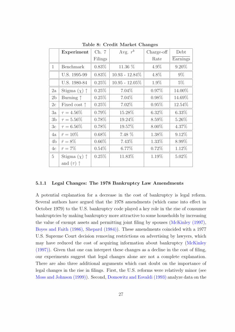
Table 8: Credit Market Changes

Experiment Ch. 7 Avg. rb Charge-off Debt

Filings Rate Earnings

1 Benchmark 0.83% 11.36 % 4.9% 9.20%

U.S. 1995-99 0.83% 10.93 - 12.84% 4.8% 9%

U.S. 1980-84 0.25% 10.95 - 12.05% 1.9% 5%

2a Stigma (χ) ↑ 0.25% 7.04% 0.97% 14.00%

2b Burning ↑ 0.25% 7.04% 0.98% 14.69%

2c Fixed cost ↑ 0.25% 7.02% 0.95% 12.54%

3a τ = 4.56% 0.79% 15.28% 6.32% 6.33%

3b τ = 5.56% 0.78% 19.24% 8.59% 5.26%

3c τ = 6.56% 0.78% 19.57% 8.00% 4.37%

4a r = 10% 0.68% 7.48 % 1.38% 9.12%

4b r = 8% 0.66% 7.43% 1.33% 8.99%

4c r = 7% 0.54% 6.77% 0.72% 1.12%

5 Stigma (χ) ↑ 0.25% 11.83% 1.19% 5.02%

and (τ) ↑

5.1.1 Legal Changes: The 1978 Bankruptcy Law Amendments

A potential explanation for a decrease in the cost of bankruptcy is legal reform.

Several authors have argued that the 1978 amendments (which came into effect in

October 1979) to the U.S. bankruptcy code played a key role in the rise of consumer

bankruptcies by making bankruptcy more attractive to some households by increasing

the value of exempt assets and permitting joint filing by spouses (McKinley (1997),

Boyes and Faith (1986), Shepard (1984)). These amendments coincided with a 1977

U.S. Supreme Court decision removing restrictions on advertising by lawyers, which

may have reduced the cost of acquiring information about bankruptcy (McKinley

(1997)). Given that one can interpret these changes as a decline in the cost of filing,

our experiments suggest that legal changes alone are not a complete explanation.

There are also three additional arguments which cast doubt on the importance of

legal changes in the rise in filings. First, the U.S. reforms were relatively minor (see

Moss and Johnson (1999)). Second, Domowitz and Eovaldi (1993) analyze data on the

27

characteristics of bankrupts before and after the 1978 amendments, and conclude that

the amendments did not play a significant role in the rise in consumer bankruptcies.

Finally, there were no corresponding changes to the bankruptcy law in Canada, and

yet filing rates in Canada also increased dramatically.31

5.2 Decline in Lending Costs

Technological progress has had a significant effect on the working of consumer credit

markets. One way of capturing many important elements of these changes in the

model is via a decline in the transactions cost of making loans (the wedge between

the safe borrowing rate and the saving rate). This has a direct counterpart in the

observed decline in the costs of processing consumer loans due to increased use of

credit scoring (Mester (1997)). Financial innovations such as securitization have also

lowered the cost of funds to financial intermediaries (Furletti (2002)), which in our

framework translates into a reduced transactions cost of borrowing. An additional

possibility is that increased competition in the banking sector led to a decline in the

profits of credit card providers and thus reduced the wedge between the borrowing

and lending rate.32

Although there are no direct measurements of the transaction costs, the follow-

ing back-of-the-envelope calculation gives a rough idea of the magnitude. In the

model, charge-offs, the borrowing interest rate and the risk-free borrowing rate are

tied together by the zero profit condition. Abstracting from aggregation issues due to

borrower heterogeneity, the charge-offs are roughly equal to r−(rs+τ)1+r

, where r denotes

the average borrowing interest rate, rs is the saving interest rate and τ is the wedge

between the saving rate and the safe borrowing rate. We can use this relationship

to back out the implied wedge. Based on the data from the end of the late 1990s

(charge-offs = 0.048, rs = 0.0344, and r ∈ [0.1093, 0.1284]), the implied borrowing

wedge is between 2.2 and 4 percent.33 Using the early 1980s data instead gives a τ of

between 5.4 and 6.8 percent. The implied decline in the transactions cost is roughly

3 percentage points.

31There are two caveats. First, there were potentially important administrative changes that mayhave increased access to the bankruptcy system for low income households during the early 1970s.Second, the flattening of Canadian bankruptcy filings after the tightening of the code in 1997 suggestthat legislative changes can have a significant impact upon filings (Ziegel (1997)).

32Dick and Lehnert (2006) argue that the removal of barriers to interstate branch banking increasedcompetition between banks.

33Note that our calibrated τ = 2.56% falls right into this range.

28

We report the results for increases in the transaction cost of lending centered

about our back-of-the-envelope estimate (of two, three and four percentage points) in

rows 3a, 3b, 3c in Table 8. Surprisingly, none of these changes has a large effect on

filings. However, variations in the transaction cost of lending have a large effect upon

aggregate borrowing, the average borrowing interest rate, and the charge-off rate.

For all three experiments, the increase in average borrowing interest rates exceeds

the increase in the risk-free borrowing interest rate. This is due to the fact that lower

risk households reduce their borrowing, which leads to an increase in the average

risk premium on lending. Our interpretation of these results is that this channel

of financial market innovations is unlikely to have played a large direct role in the

increase in filings, but is an important factor in the rise in unsecured borrowing.

These results are quite different from Athreya (2004), who reports that reductions

in the transaction cost of lending can generate a substantial increase in both filings

and debt. The small effect we find on filings stems from two differences between our

models. First, Athreya (2004) abstracts from expense uncertainty, which drives a large

fraction of the defaults in our framework. Expense uncertainty implies that reductions

in the cost of borrowing not only encourage more borrowing – which makes households

more likely to file for bankruptcy given shocks – but also makes borrowing so as to

pay off expense shocks over time more attractive relative to filing for bankruptcy.

Secondly, the life cycle nature of our model makes risky young borrowers less sensitive

to changes in borrowing rates, and thus generates their continued participation when

the transaction costs are high.

One other issue worth highlighting is that we assume that the risk free rate is

fixed in all of our experiments, while the transaction cost of lending varies. Our

rationale is that the return to saving in the model is a proxy for the return on capital

in the economy, which McGrattan and Prescott (2003) argue has remained roughly

constant over 1980-2000. In effect, we take the view that the opportunity cost of funds

to the lenders should be equal to the return on capital, and load all of the costs of

intermediation into the τ . To check the robustness of this approach, we also undertook

experiments where we increased the risk-free rate (rs) while holding the transaction

cost of lending (τ) fixed. As one would expect, although a slightly smaller increase

in rs is needed to generate the same decrease in borrowing as a given change in τ ,

these experiments yielded similar results to those reported in Table 8. This suggests

that whether borrowing became cheaper due to efficiency gains in the lending sector,

or due to other macroeconomic factors that lowered the aggregate interest rate is not

important for our results. Instead, what is key is that credit markets changes led to

29

an effective reduction in borrowing costs for consumers.

5.3 Removal of Usury Laws

Until the late 1970’s, most states imposed (tight) ceilings on nominal interest rates

for consumer loans. These laws were relaxed in the early 1980s as a result of the

1978 Supreme Court decision involving Marquette National Bank of Minneapolis to

permit banks from Nebraska to offer loans to residents of Minnesota at rates in excess

of the maximum allowed under Minnesota legislation. This ruling effectively removed

the ability of individual states to regulate interest rates of lenders located in other

states. Subsequently in the early 1980s, large credit card issuers relocated to states

(notably Delaware and South Dakota) with the highest interest rate ceiling (Evans

and Schmalnsee (1999)). This was followed by a rapid growth in high interest rate

credit card debt, which coincided with the rise in consumer bankruptcies. This has

led some to suggest that the Marquette decision contributed to the rise in bankruptcy

by facilitating the expansion of credit to riskier borrowers.

We report the results of numerical experiments for three alternative ceilings in

Table 8, all of which lie below the average borrowing interest rate in the benchmark

economy and above the risk-free lending rate of 6% (experiments 4a-4c). Even a

very tight interest rate ceiling of 7% can only account for roughly half of the rise in

filings. This result is driven by the fact that bankruptcies in the model are caused

by bad realizations of expense and income uncertainty. A tight borrowing constraint

dramatically reduces borrowing (by preventing the extension of credit to “risky”

borrowers and placing tight restrictions on the amount that can be borrowed). Lower

borrowing in turn reduces the incentive for households to default in response to bad

realizations of expense and income shocks. Offsetting this is the fact that tight

borrowing constraints associated with low interest rate ceilings significantly limits

households ability to borrow to smooth negative shocks. This in turn pushes some

households who would not have defaulted in the absence of the tight interest rate

ceiling to default, and this limits the effect of interest rate ceilings on defaults.

The numerical experiments indicate that the interest rate deregulation story is not

consistent with observed interest rates. While a relaxation of the ceiling is consistent

with a rise in the debt-income ratio, it also implies a substantial increase in the

average borrowing interest rates. In the data, however, there appears to be little

change in the average borrowing interest rate.

30

There are two additional observations which cast some doubt on the importance of

usury laws. First, Canada has also experienced a rapid rise in consumer bankruptcies

but did not experience a deregulation of credit markets around the same time (see

also Ellis (1998)).34 Second, it is unclear whether interest rate ceilings were effectively

binding in the United States. For example, Peterson (1983) argues that one way

around interest rate ceilings is for the seller of a good to sell at a higher price on credit.

He examines data from 1979 for four states with different interest rate ceilings, and

finds that the state with the lowest ceiling (Arkansas) had a higher share of installment

credit offered directly by retailers than other states. This argument is consistent with

the observed shift of credit away from store-based to general purpose lending after

the removal of interest rate ceilings.

Our conclusion is that while the Marquette decision may have contributed indi-

rectly to the rise in bankruptcies by permitting continued lending to high risk con-

sumers, it was not in itself a significant cause of the rise in filings.

5.4 Can a Combination of Credit Market Channels Generate

the Rise?

Thus far we have considered the impact of changes in each of the three credit market

channels separately. However, credit market innovations likely affected all of these

channels. Moreover, the results reported above for each channel individually suggest

that credit market innovations which made both borrowing and filing less costly could

lead to a large extension of debt as well as a dramatic increase in filings. Could credit

market innovations which led to reduction in both the transaction cost τ and the cost

of bankruptcy χ account for the observed experience?

The answer is yes. Experiment 5 in Table 8 reports the results of an increase in

the transaction cost of 4.5 percentage points (from 2.56% to 7.06%) and an increase

of the stigma parameter to roughly three quarters of its value in the “stigma only”

experiment (line 2a in Table 8). With these values, the model closely replicates the

level of filings, the average borrowing interest rate and the debt-to-earnings ratio

observed in the early 1980s. The model also predicts a sizable increase in the charge-

off rate from the 1980s to the late 1990s in line with the data: an increase from 1.2%

to 4.9% in the model, compared to a slightly lower increase in the data, from 1.9%

34Interest rate ceilings on bank loans were formally removed in Canada through the Bank Act of1967, although these ceilings were largely ineffective, as borrowers were free to “voluntarily” agree topay higher interest rates in the form of an upfront charge at the time of the loan (Scholnick (2000)).

31

to 4.8%.

The intuition for the success of this experiment is as follows. The reduction in

the cost of filing makes bankruptcy more attractive which decreases the bond price

schedule (i.e., interest rates are higher for any level of borrowing). This leads to a

decline in borrowing and an increase in average borrowing interest rates (see exper-

iment 2 in Table 8). The fact that a decline in the transactions costs of lending can

offset the changes in interest rates and borrowing is not obvious. The direct effect

of a lower τ is to increase the bond price schedule, thereby increasing desired bor-

rowing by households. The lower interest rate schedule reduces the cost of repaying

one’s loans for any level of debt, which increases the value of repaying relative to

the value of bankruptcy. The lower interest rate schedule also increases the cost of

being excluded from borrowing during the bankruptcy period. The overall effect is to

increase both the fraction of young households who borrow and the amount borrowed

by borrowers. Due to these forces, lower transaction costs significantly increase bor-

rowing while lowering the incentive to default for a given level of borrowing. As a

result, the realized average default rate is only slightly changed by the change in the

transactions cost.

6 Decomposing the Relative Importance of Uncer-

tainty and Credit Market Channels

The results from the previous two sections suggest that credit market changes are

largely responsible for the rise in filings, while uncertainty plays only a minor role.

However, in principle, the various channels might interact and reinforce each other.

To better evaluate the relative importance of credit market changes, we now analyze

a combination of uncertainty and credit market changes simultaneously. This allows

us to assess the contribution of each story, while allowing for interaction effects.

We incorporate two uncertainty stories: an increase in expense uncertainty and an

increase in transitory income uncertainty. A reasonable upper bound on the change

in expense uncertainty is that the probabilities in the early 1980s were roughly 85%

of those the late 1990s. We thus scale down the benchmark probabilities of expense

shocks by 0.85. To capture changes in income volatility, we scale down the variance

of the transitory shock by 25% (which is at the upper limit of the values suggested

by Heathcoate, Storesletten, and Violante (2004)). Given these changes, we choose

32

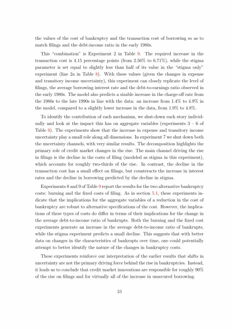
the values of the cost of bankruptcy and the transaction cost of borrowing so as to

match filings and the debt-income ratio in the early 1980s.

This “combination” is Experiment 2 in Table 9. The required increase in the

transaction cost is 4.15 percentage points (from 2.56% to 6.71%), while the stigma

parameter is set equal to slightly less than half of its value in the “stigma only”

experiment (line 2a in Table 8). With these values (given the changes in expense

and transitory income uncertainty), this experiment can closely replicate the level of

filings, the average borrowing interest rate and the debt-to-earnings ratio observed in

the early 1980s. The model also predicts a sizable increase in the charge-off rate from

the 1980s to the late 1990s in line with the data: an increase from 1.4% to 4.9% in

the model, compared to a slightly lower increase in the data, from 1.9% to 4.8%.

To identify the contribution of each mechanism, we shut-down each story individ-

ually and look at the impact this has on aggregate variables (experiments 3 – 6 of

Table 9). The experiments show that the increase in expense and transitory income

uncertainty play a small role along all dimensions. In experiment 7 we shut down both

the uncertainty channels, with very similar results. The decomposition highlights the

primary role of credit market changes in the rise. The main channel driving the rise

in filings is the decline in the costs of filing (modeled as stigma in this experiment),

which accounts for roughly two-thirds of the rise. In contrast, the decline in the

transaction cost has a small effect on filings, but counteracts the increase in interest

rates and the decline in borrowing predicted by the decline in stigma.

Experiments 8 and 9 of Table 9 report the results for the two alternative bankruptcy

costs: burning and the fixed costs of filing. As in section 5.1, these experiments in-

dicate that the implications for the aggregate variables of a reduction in the cost of

bankruptcy are robust to alternative specifications of the cost. However, the implica-

tions of these types of costs do differ in terms of their implications for the change in

the average debt-to-income ratio of bankrupts. Both the burning and the fixed cost

experiments generate an increase in the average debt-to-income ratio of bankrupts,

while the stigma experiment predicts a small decline. This suggests that with better

data on changes in the characteristics of bankrupts over time, one could potentially

attempt to better identify the nature of the changes in bankruptcy costs.

These experiments reinforce our interpretation of the earlier results that shifts in

uncertainty are not the primary driving force behind the rise in bankruptcies. Instead,

it leads us to conclude that credit market innovations are responsible for roughly 90%

of the rise on filings and for virtually all of the increase in unsecured borrowing.

33

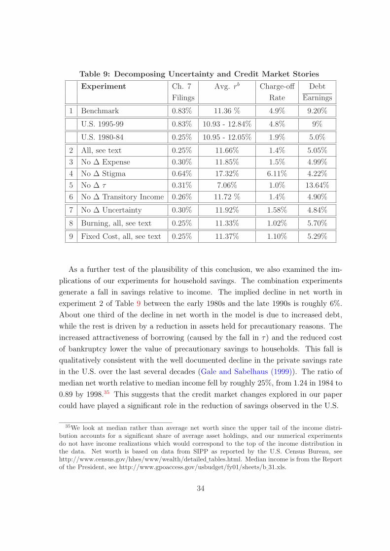
Table 9: Decomposing Uncertainty and Credit Market Stories

Experiment Ch. 7 Avg. rb Charge-off Debt

Filings Rate Earnings

1 Benchmark 0.83% 11.36 % 4.9% 9.20%

U.S. 1995-99 0.83% 10.93 - 12.84% 4.8% 9%

U.S. 1980-84 0.25% 10.95 - 12.05% 1.9% 5.0%

2 All, see text 0.25% 11.66% 1.4% 5.05%

3 No ∆ Expense 0.30% 11.85% 1.5% 4.99%

4 No ∆ Stigma 0.64% 17.32% 6.11% 4.22%

5 No ∆ τ 0.31% 7.06% 1.0% 13.64%

6 No ∆ Transitory Income 0.26% 11.72 % 1.4% 4.90%

7 No ∆ Uncertainty 0.30% 11.92% 1.58% 4.84%

8 Burning, all, see text 0.25% 11.33% 1.02% 5.70%

9 Fixed Cost, all, see text 0.25% 11.37% 1.10% 5.29%

As a further test of the plausibility of this conclusion, we also examined the im-

plications of our experiments for household savings. The combination experiments

generate a fall in savings relative to income. The implied decline in net worth in

experiment 2 of Table 9 between the early 1980s and the late 1990s is roughly 6%.

About one third of the decline in net worth in the model is due to increased debt,

while the rest is driven by a reduction in assets held for precautionary reasons. The

increased attractiveness of borrowing (caused by the fall in τ) and the reduced cost

of bankruptcy lower the value of precautionary savings to households. This fall is

qualitatively consistent with the well documented decline in the private savings rate

in the U.S. over the last several decades (Gale and Sabelhaus (1999)). The ratio of

median net worth relative to median income fell by roughly 25%, from 1.24 in 1984 to

0.89 by 1998.35 This suggests that the credit market changes explored in our paper

could have played a significant role in the reduction of savings observed in the U.S.

35We look at median rather than average net worth since the upper tail of the income distri-bution accounts for a significant share of average asset holdings, and our numerical experimentsdo not have income realizations which would correspond to the top of the income distribution inthe data. Net worth is based on data from SIPP as reported by the U.S. Census Bureau, seehttp://www.census.gov/hhes/www/wealth/detailed tables.html. Median income is from the Reportof the President, see http://www.gpoaccess.gov/usbudget/fy01/sheets/b 31.xls.

34

7 Conclusion

In this paper, we quantitatively evaluate the extent to which the most commonly

offered explanations can account for the rise in personal bankruptcy filings as well

as the increase in unsecured consumer debt relative to disposable income, the lack

of change in average borrowing interest rates, and the rise in charge-off rates. Our

results suggest that uncertainty-based stories cannot account for the rise in consumer

bankruptcies and increase in unsecured borrowing. Instead, our experiments suggest

that at least three quarters of the rise in filings are due to changes in credit markets.

Hence, our paper suggests that credit market innovations which have reduced the

cost (“stigma”?) of bankruptcy and as well as the cost of borrowing have played an

essential role in the rise of bankruptcies and unsecured consumer borrowing.

These results are different from various papers which have argued for a monocausal

explanation of the rise. The spirit of our results are close to those of Athreya (2004)

and Moss and Johnson (1999), in that we view credit market changes as playing

the key role in the rise. However, our results suggest that a decline in the cost of

bankruptcy plays a much more important role in the rise in filings than these papers

would suggest. Of course, this finding leaves open the question of what exactly has

caused the decline in the cost of bankruptcy. We believe that endogenizing these

bankruptcy costs is an important challenge for future research. One hypothesis is

that this cost has declined because of the reduced cost of accessing credit markets

after bankruptcy – a story documented by Staten (1993). This could be due to

improved forecasting of a person’s bankruptcy risk caused by technological innovation

in the financial sector. With little information about a debtor’s “type,” bankruptcy

is an important signal to creditors about future default risk. However, if banks have

full information about a creditor ex-ante, then bankruptcy is simply an instance of

bad luck and does not contain further information about a person’s type, in which

case, bankruptcy should not increase the person’s cost of borrowing. We therefore

believe that further work along the lines of Chatterjee, Corbae, and Rios-Rull (2006)

is important to improve our understanding of the working of consumer credit markets.

References

Adda, J., and R. Cooper (2003): Dynamic Economics. MIT Press, Cambridge,

Massachusetts.

35

Athreya, K. (2002): “Welfare Implications of the Bankruptcy Reform Act of 1999,”

Journal of Monetary Economics, 49, 1567–1595.

(2004): “Shame as it Ever Was: Stigma and Personal Bankruptcy,” Federal

Reserve Bank of Richmond Economic Quarterly, 90(2), 1–19.

(2005): “Equilibrium Models of Personal Bankruptcy: A Survey,” Federal

Reserve Bank of Richmond Economic Quarterly, 91(2), 73–98.

Ausubel, L. (1991): “The Failure of Competition in the Credit Card Model,” Amer-

ican Economic Review, 81(4), 50–81.

Baird, D. G. (2007): “Technology, Information and Bankruptcy,” Univrsity of Illi-

nois Law Review, pp. 305–322.

Barron, J. M., G. Elliehausen, and M. E. Staten (2000): “Monitoring the

Household Sector with Aggregate Credit Bureau Data,” Business Economics.

Barron, J. M., and M. Staten (2003): “The Value of Comprehensive Credit

Reports,” in Credit Reporting Systems and the International Economy, ed. by M. J.

Miller, pp. 273–310. MIT Press.

Berger, A. (2003): “The Economic Effects of Technological Progress: Evidence

from the Banking Industry,” Journal of Money, Credit and Banking, 35(2), 141–

176.

Bermant, G., and E. Flynn (1999): “Incomes, Debts and Repayment Capaci-

ties of Recently Discharged Chapter 7 Debtors,” American Bankruptcy Institute,

http://www.usdoj.gov/ust/press/articles/ch7trends-01.htm.

Blundell, R., L. Pistaferri, and I. Preston (2005): “Consumption Inequality

and Partial Insurance,” Stanford University, mimeo.

Boyes, W., and R. L. Faith (1986): “Some Effects of the Bankruptcy Reform Act

of 1978,” Journal of Law and Economics, XXIX, 139–149.

Buckley, F., and M. F. Brinig (1998): “The Bankruptcy Puzzle,” The Journal

of Legal Studies, XXVII, 187–207.

Butrica, B. A., H. M. Iams, and K. E. Smith (2004): “The Changing Impact

of Social Security on Retirement Income in the United States,” Social Secuirty

Bulletin, 65(3), 1–13.

36

Cain, J. M. (1997): “Proving Fraud in Credit Card Dischargeability Actions: A

Permanent State of Flux,” Commercial Law Journal, 102(3), 233–255.

Carroll, C., and A. Samwick (1997): “The Nature of Precautionary Wealth,”

Journal of Monetary Economics, 40(4), 41–71.

Center for Medicare and Medicaid Services (2005): “National Health Ex-

penditures Aggregate and per Capita Amounts, Percent Distribution, and Average

Annual Percent Growth, by Source of Funds: Selected Calendar Years 1980-2003,”

http://www.cms.hhs.gov/statistics/nhe/historical/.

Chatterjee, S., D. Corbae, M. Nakajima, and J.-V. Rios-Rull (2005): “A

Quantitative Theory of Unsecured Consumer Credit with Risk of Default,” Federal

Reserve Bank of Philadelphia Working Paper 05-18.

Chatterjee, S., D. Corbae, and J.-V. Rios-Rull (2006): “A Finite-Life

Private-Information Theory of Unsecured Debt,” University of Texas at Austin,

mimeo.

Dick, A. A., and A. Lehnert (2006): “Personal Bankruptcy and Credit Market

Competition,” mimeo.

Domowitz, I., and T. L. Eovaldi (1993): “The Impact of the Bankruptcy Re-

form Act of 1978 on Consumer Bankruptcy,” The Journal of Law and Economics,

XXXVI, 803–835.

Domowitz, I., and R. L. Sartain (1999): “Determinants of the Consumer

Bankruptcy Decision,” The Journal of Finance, 54(1), 403–420.

Dynan, K., K. Johnson, and K. Pence (2003): “Recent Changes to a Measure

of U.S. Household Debt Service,” Federal Reserve Bulletin, pp. 417–426.

Ellis, D. (1998): “The Effect of Consumer Interest Rate Deregulation on Credit

Card Volumes, Charge-Offs and the Personal Bankruptcy Rate,” FDIC Bank

Trends, 98(5).

Evans, D., and R. Schmalnsee (1999): Paying with Plastic: The Digital Revolu-

tion in Buying and Borrowing. MIT Press, Cambridge, Massachusetts.

Fay, S., E. Hurst, and M. j. White (2002): “The Household Bankruptcy Deci-

sion,” American Economic Review, 92(3), 706–718.

37

Furletti, M. (2002): “An Overview of Credit Card Asset-Backed Securities,” Fed-

eral Reserve Bank of Philadelphia Payment Cards Center Discussion Paper.

(2003a): “Credit Card Pricing Devlopments and Their Disclosure,” Federal

Reserve Bank of Philadelphia Payments Card Center Discussion Paper.

(2003b): “Measuring Credit Card Industry Chargeoffs: A Review of Sources

and Methods,” Federal Reserve Bank of Philadelphia Discussion Paper.

Gale, W. G., and J. Sabelhaus (1999): “Perspectives on the Household Savings

Rate,” The Brookings Institution, mimeo.

Goldstein, J. (1999): “The Leveling of Divorce in the United States,” Demography,

36(3), 409–414.

Gourinchas, P.-O., and J. Parker (2002): “Consumption over the Life Cycle,”

Econometrica, 70(1), 47–89.

Gross, D., and N. Souleles (2002): “An Empirical Anaylsis of Personal

Bankruptcy and Delinquency,” The Review of Financial Studies, 15(1), 319–347.

Hacker, J. S. (2006): The Great Risk Shift. Oxford University Press, Toronto,

Ontario.

Heathcoate, J., K. Storesletten, and G. Violante (2004): “The Cross-

Sectional Implications of Rising Wage Inequality in the United States,” New York

University, mimeo.

Hubbard, R., J. Skinner, and S. P. Zeldes (1994): “The Importance of Pre-

cautionary Motives in Explaining Individual and Aggregate Saving,” Carnegie-

Rochester Conference Series on Public Policy, 40, 59–125.

Kambourov, G., and I. Manovskii (2004): “Occupational Mobility and Wage

Inequality,” mimeo.

Laibson, D., J. Tobacman, and A. Repetto (2000): “A Debt Puzzle,” NBER

Working Paper, 7879.

Li, W., and P.-D. Sarte (2006): “U.S. consumer bankruptcy choice: The Im-

portance of General Equilibrium Effects,” Journal of Monetary Economics, 53(3),

613–631.

38

Livshits, I., J. MacGee, and M. Tertilt (2003): “Consumer Bankruptcy: A

Fresh Start,” Federal Reserve Bank of Minneapolis Working Paper.

(2007): “Consumer Bankruptcy: A Fresh Start,” American Economic Re-

view, 97, 402–418.

Lown, J. M., and B. R. Rowe (2002): “A Profile of Consumer Bankruptcy Peti-

tioners,” mimeo, Utah State University.

Luckett, C. (2002): “Personal Bankruptcies,” in The Impact of Public Policy on

Consumer Credit, ed. by T. Durkin, and M. Staten, pp. 69–102. Kluwer Academic

Punlishers.

McGrattan, E. R., and E. C. Prescott (2003): “Average Debt and Equity

Returns: Puzzling?,” American Economic Review Papers and Proceedings, 93(2),

392–397.

McKinley, V. (1997): “Ballooning Bankruptcies,” Regulation, pp. 33–40.

Mecham, L. R. (2004): Bankruptcy Basics. Administrative Office of the United

States Courts.

Meghir, C., and L. Pistaferri (2004): “Income Variance Dynamics and Hetero-

geneity,” Econometrica, 72(1), 1–32.

Mester, L. (1997): “What’s the Point of Credit Scoring,” Federal Reserve Bank of

Philadelphia Business Review, pp. 3–16.

Moffitt, R., and P. Gottschalk (2002): “Trends in the Transitory Variance of

Earnings in the United States,” Economic Journal, 112(478), C68–C73.

Moss, D. A., and G. A. Johnson (1999): “The Rise of Consumer Bankruptcy:

Evolution, Revolution or Both?,” American Bankruptcy Law Journal, 73, 311–352.

Narajabad, B. N. (2006): “Information Technology and the Rise of Household

Bankruptcy,” Job Market paper, University of Texas at Austin.

National Bankruptcy Review Commission (1997): “Bankruptcy: The Next

Twenty Years. Final Report of the Bankruptcy Review Commission,” Discussion

paper, http://www.nbrc.gov/reportcont.html.

39

Peterson, R. L. (1983): “Usury Laws and Cosnumer Credit: A Note,” The Journal

of Finance, pp. 1299–1304.

Pollak, O. B. (1997): “Gender and Bankruptcy: An Empirical Analysis of Evolving

Trends in Chapter 7 and Chapter 13 Bankruptcy Filings 1967-1997,” Commercial

Law Journal, 102(3), 333–228.

Scholnick, B. (2000): “Regulation, Competition and Risk in the market for Credit

Cards,” Canadian Public Policy, XXVI(2), 171–181.

Shepard, L. (1984): “Personal Failures and the Bankruptcy Reform Act of 1978,”

Journal of Law and Economics, XXVII, 419–437.

Staten, M. (1993): “The Impact of Post-Bankruptcy Credit on the Number of

Personal Bankruptcies,” Credit Research Centre Working Paper No 58.

Storesletten, K., C. Telmer, and A. Yaron (2004): “Consumption and Risk

Sharing over the Life Cycle,” Journal of Monetary Economics, 51, 609–633.

Sullivan, T., D. Thorne, and E. Warren (2001): “Young, Old and In Between:

Who Files for Bankruptcy?,” Norton Bankruptcy Law Adviser.

Sullivan, T., and E. Warren (1999): “The Changing Demographics of

Bankruptcy,” Norton Bankruptcy Law Adviser.

Sullivan, T. A., E. Warren, and J. L. Westbrook (1999): As We Forgive Our

Debtors: Bankruptcy and Consumer Credit in America. Beard Books, Washington,

D.C.

(2000): The Fragile Middle Class. Yale University Press, New Haven and

London.

U.S. Census Bureau (2000): Statistical Abstract of the United States,Washington,

D.C.

VISA USA (1996): “Consumer Bankruptcy: Causes and Implications,” VISA Con-

sumer Bankruptcy Reports.

Warren, E. (2002): “Financial Collapse and Class Status: Who Goes Bankrupt?,”

Osgoode Hall Law Journal, 41, 115–146.

40

Warren, E., and A. Warren Tyagi (2003): The Two Income Trap: Why Middle-

Class Mothers & Fathers Are Going Broke (With Surprising Solutions That Will

Change Our Children’s Futures). Basic Books, New York.

Wells, W., J. Kurtz, and R. Calhoun (1991): “The Implementation of

Bankrupcty Code Section 707(b): The Law and the Reality,” Cleveland State Law

Review, pp. 15–48.

White, M. (2007): “Bankruptcy Reform and Credit Cards,” NBER Working Paper

No. 13265.

Ziegel, J. S. (1997): “Canadian Perspectives on the Challenges of Consumer

Bankruptcy,” Journal of Consumer Policy, 20(2), 199–221.

Zywicki, T. J. (2005): “Institutions, Incentives, and Consumer Bankruptcy Re-

form,” George Mason University School of Law Law and Economics Working Paper

05-07.

41

A Figures

Figure 1: Bankrupts per 1000 18-64.

U.S. Consumer bankruptcies are the sum of non-business Chapter 7 and Chapter

13 filings. The data from 1979 and before is from Table 1 of McKinley (1997), while

the number of filings from 1980 to 2004 are from the ABI website. The denominator

is the estimate of the U.S. population between the ages of 18 and 64 as of July 1.

Canada: Consumer Bankruptcies plus consumer proposals. The numerator is the

total number of bankruptcy petitions filed. Joint filing is permitted when two people

have interrelated finances, so this may understate the total number of bankrupts.

Figures 2 and 3: Debt as % of Disposable Income

Total debt is the summation of mortgage debt and consumer debt. Mortgage

debt is from the Flow of Funds of Account, Table D.3. The mortgage data gives the

end of period balance outstanding quarterly, and has been converted to annual by

averaging. Consumer credit is the summation of revolving and nonrevolving consumer

credit balances outstanding reported in G.19. The original data was monthly, and was

converted to annual by averaging. The data we report is based on the 2004 revision

and includes student loans outstanding in nonrevolving credit. Personal disposable

income is from the Bureau of Economic Analysis, Table 2.1. Personal Income and Its

Disposition [Billions of dollars].

The unsecured credit measure in Figure 3 over 1983-1999 was constructed as fol-

lows. Before 1999, G.19 reported consumer credit in the following three categories: re-

volving, automobile (non-revolving) and other nonrevolving (after 1999, G.19 reports

consumer credit as either revolving or nonrevolving, which is why our constructed

series ends in 1999). To estimate unsecured consumer credit, we: (1) Constructed

a non-automobile non-revolving debt measure by subtracting the automobile debt

series from the updated non-revolving series (this series contains student loans issued

by the federal government); (2) Used linear extrapolation to construct a measure of

the fraction of non-auto non-revolving debt that is personal using the values reported

by Dynan, Johnson, and Pence (2003) from the SCF for 1983, 1989, 1992, 1995 and

1998; and (3) Finally, we construct our measure of unsecured consumer credit by

summing: revolving + non-auto non-revolving * fraction personal.

42

B Surveys of Bankrupts

While there are several empirical studies of U.S. bankrupts, one must be careful in

comparing them due to differences in their approach to sample selection. The most

well known are those associated with the work of Sullivan, Warren, and Westbrook

(1999) and Sullivan, Warren, and Westbrook (2000).

1. Sullivan, Warren, and Westbrook (1999): The 1981 study involved a sample of

1,550 debtors from ten judicial districts in three states: Illinois, Pennsylvania

and Texas. This study was based upon what was reported in the bankruptcy

file. They converted their raw data to 1997 $ using the CPI.

2. Sullivan, Warren, and Westbrook (2000): This is a 1991 study of bankrupts in

16 federal districts in Illinois, Pennsylvania, Texas, California and Tennessee. In

this study, written surveys were used to collect information on each bankrupt.

In addition, financial data on bankrupts in five of the districts were collected

from court records. They converted their raw data to 1997 $ using the CPI.

3. Based on court records, Domowitz and Sartain (1999) examine a sample of

households who filed for bankruptcy before and after the 1978 Bankruptcy Law

Amendments came into effect. Their data includes 580 Chapter 7 households

who filed for bankruptcy between October 1978 and March 1979 and 670 Chap-

ter 7 bankrupts who filed between April and September 1980 from Southern and

Eastern New York, Southern Ohio, Eastern Kentucky and Central California.

They report that mean income was between $24,300 and $26,600 (in 1991 $).

4. Bermant and Flynn (1999) looked at a sample of approximately 2000 chapter 7

cases closed during the first half of 1998. They restricted attention to no-asset

chapter 7 cases, and report that of the 975,370 consumer chapter 7 cases filed

in 1997 all but 10,000 were closed as no-asset cases.

5. Lown and Rowe (2002) examine a sample of bankrupts in Utah from 1997.

Their data is based on a sample of 1486 Chapter 7 and 1081 Chapter 13 filed

in U.S. Bankruptcy Court in Utah in 1997. Their data indicates that the av-

erage and median debts of chapter 13 filers were larger than those of chapter

7 filers. However, the median and average debt-income ratios were lower since

the average incomes of chapter 13 filers were higher than those of chapter 7.

43

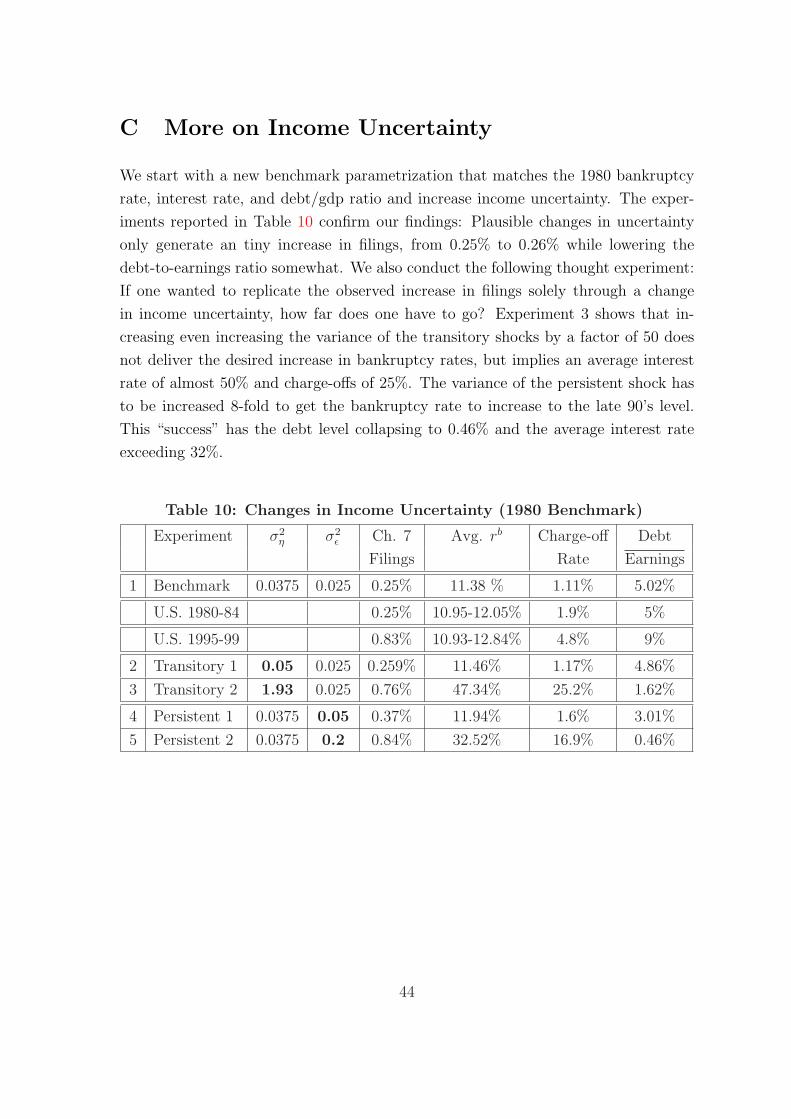
C More on Income Uncertainty

We start with a new benchmark parametrization that matches the 1980 bankruptcy

rate, interest rate, and debt/gdp ratio and increase income uncertainty. The exper-

iments reported in Table 10 confirm our findings: Plausible changes in uncertainty

only generate an tiny increase in filings, from 0.25% to 0.26% while lowering the

debt-to-earnings ratio somewhat. We also conduct the following thought experiment:

If one wanted to replicate the observed increase in filings solely through a change

in income uncertainty, how far does one have to go? Experiment 3 shows that in-

creasing even increasing the variance of the transitory shocks by a factor of 50 does

not deliver the desired increase in bankruptcy rates, but implies an average interest

rate of almost 50% and charge-offs of 25%. The variance of the persistent shock has

to be increased 8-fold to get the bankruptcy rate to increase to the late 90’s level.

This “success” has the debt level collapsing to 0.46% and the average interest rate

exceeding 32%.

Table 10: Changes in Income Uncertainty (1980 Benchmark)

Experiment σ2η σ2

ε Ch. 7 Avg. rb Charge-off Debt

Filings Rate Earnings

1 Benchmark 0.0375 0.025 0.25% 11.38 % 1.11% 5.02%

U.S. 1980-84 0.25% 10.95-12.05% 1.9% 5%

U.S. 1995-99 0.83% 10.93-12.84% 4.8% 9%

2 Transitory 1 0.05 0.025 0.259% 11.46% 1.17% 4.86%

3 Transitory 2 1.93 0.025 0.76% 47.34% 25.2% 1.62%

4 Persistent 1 0.0375 0.05 0.37% 11.94% 1.6% 3.01%

5 Persistent 2 0.0375 0.2 0.84% 32.52% 16.9% 0.46%

44

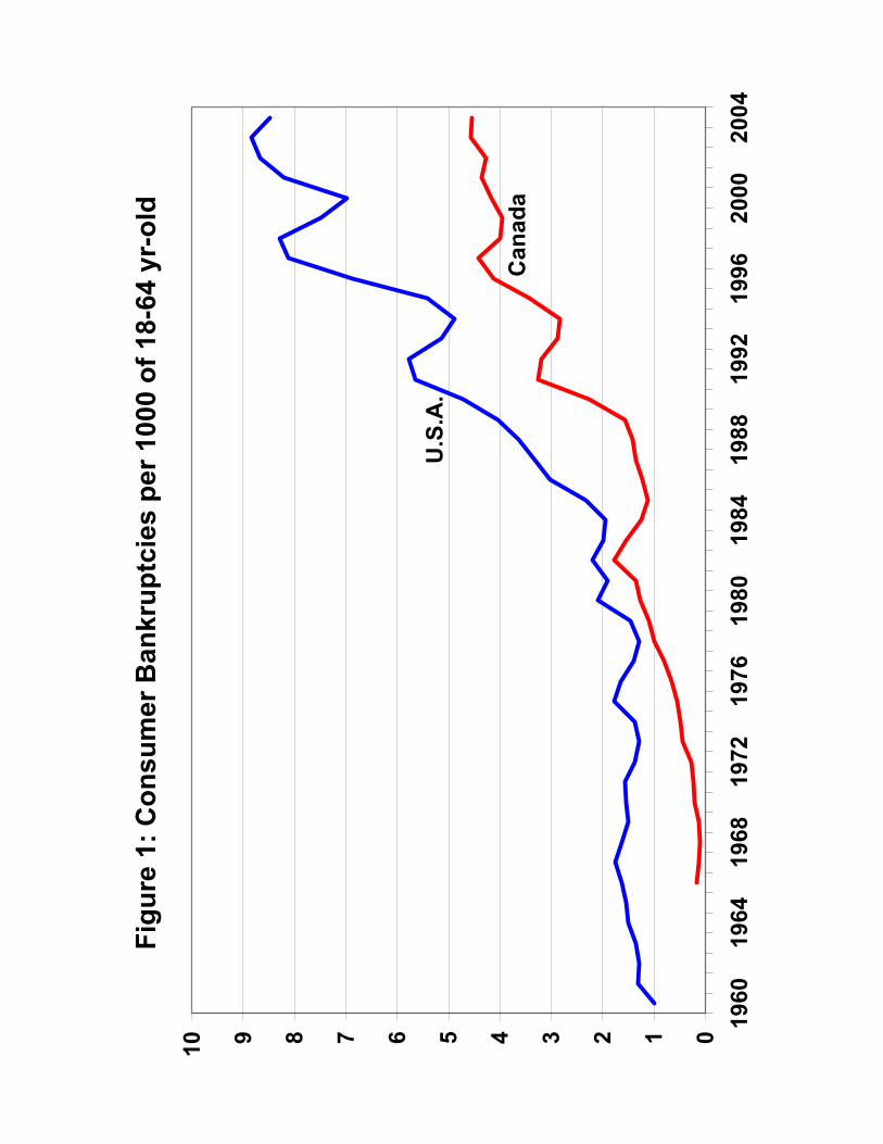
Figu

re 1

: Con

sum

er B

ankr

uptc

ies

per 1

000

of 1

8-64

yr-

old

012345678910

1960

1964

1968

1972

1976

1980

1984

1988

1992

1996

2000

2004

U.S

.A.

Can

ada

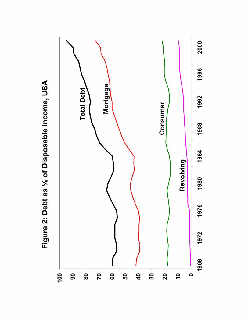
Fig

ure

2:

Deb

t as

% o

f Dis

posa

ble

Inco

me,

USA

0102030405060708090100

1968

1972

1976

1980

1984

1988

1992

1996

2000

Tota

l Deb

t

Mor

tgag

e

Rev

olvi

ng

Con

sum

er

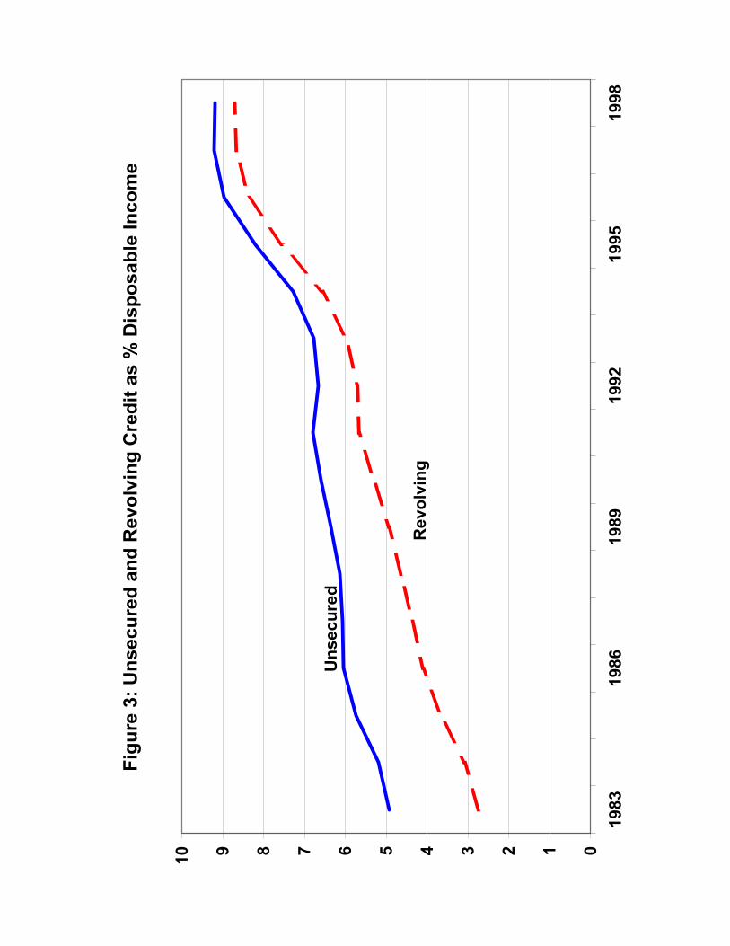
Figu

re 3

: Uns

ecur

ed a

nd R

evol

ving

Cre

dit a

s %

Dis

posa

ble

Inco

me

012345678910

1983

1986

1989

1992

1995

1998

Uns

ecur

ed

Rev

olvi

ng

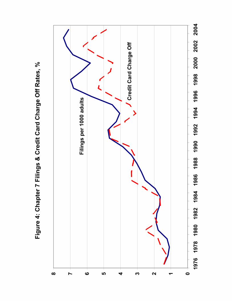
Figu

re 4

: Cha

pter

7 F

iling

s &

Cre

dit C

ard

Cha

rge

Off

Rat

es, %

012345678

1976

1978

1980

1982

1984

1986

1988

1990

1992

1994

1996

1998

2000

2002

2004

Filin

gs p

er 1

000

adul

ts Cre

dit C

ard

Cha

rge

Off

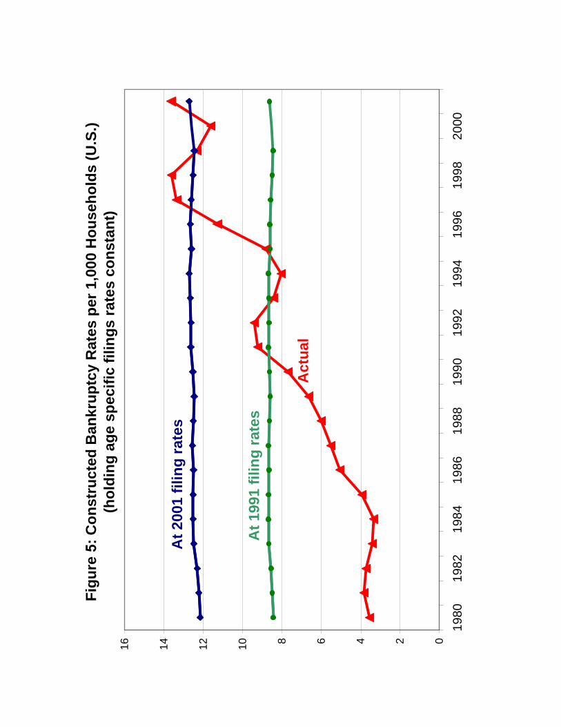
Figu

re 5

: Con

stru

cted

Ban

krup

tcy

Rat

es p

er 1

,000

Hou

seho

lds

(U.S

.)(h

oldi

ng a

ge s

peci

fic fi

lings

rate

s co

nsta

nt)

0246810121416

1980

1982

1984

1986

1988

1990

1992

1994

1996

1998

2000

Act

ual

At 1

991

filin

g ra

tes

At 2

001

filin

g ra

tes

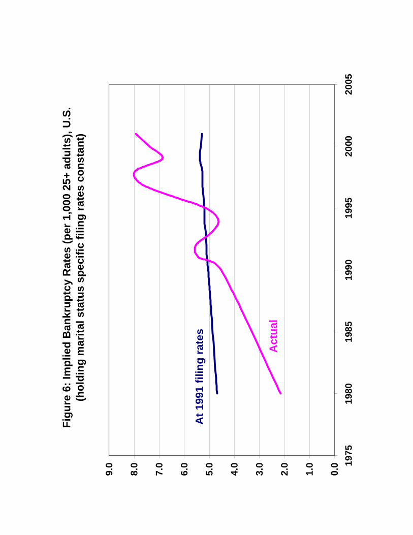
Figu

re 6

: Im

plie

d B

ankr

uptc

y R

ates

(per

1,0

00 2

5+ a

dults

), U

.S.

(hol

ding

mar

ital s

tatu

s sp

ecifi

c fil

ing

rate

s co

nsta

nt)

975

1980

1985

1990

1995

2000

2005

At 1

991

filin

g ra

tes

Act

ual

0.0

1.0

2.0

3.0

4.0

5.0

6.0

7.0

8.0

9.0 1