Accounting for the phonetic value of nonspeech sounds

By

Gregory Peter Finley

A dissertation submitted in partial satisfaction of the

requirements for the degree of

Doctor of Philosophy

in

Linguistics

in the

Graduate Division

of the

University of California, Berkeley

Committee in charge:

Professor Keith A. Johnson, ChairProfessor Susanne Gahl

Professor Frédéric E. Theunissen

Spring 2015

Abstract

Accounting for the phonetic value of nonspeech sounds

by

Gregory Peter Finley

Doctor of Philosophy in Linguistics

University of California, Berkeley

Professor Keith A. Johnson, Chair

The nature of the process by which listeners parse auditory inputs into the phonetic percepts necessary for speech understanding is still only partially understood. Different theoretical stances frame the process as either the action of ordinary auditory processes or as the workings of a specialized speech perception system or module. Evidence that speech perception is special, at least on some level, can be found in perceptual phenomena that are associated with speech processing but not observed with other auditory stimuli. These include effects known to be related to top-down linguistic influence or even to the listener’s parsing of the speaker’s articulatory gestures.

There is mounting evidence, however, that these phenomena are not always restricted to speech stimuli: some nonspeech sounds, under certain presentation conditions, participate in these phonetic processes as well. These findings are enormously relevant to the theory of speech perception, as they suggest that a sharp speech/nonspeech dichotomy is untenable. Even more promising, they offer a way of reverse-engineering those aspects of speech perception that do not have a simple psychophysical explanation by observing how they react to stimuli that are carefully controlled, and may even be missing elements that are always present in speech. Experimental work that has attempted to do so are reviewed and discussed.

Original work extending these findings for two types of nonspeech stimuli is also presented. Under the first set of experiments, compensation for coarticulation is tested on a speech fricative target with a nonspeech context vowel (a synthesized glottal source with a single formant resonance). Results show that this nonspeech does induce a reliable context effect which cannot be due to auditory contrast. This effect is weaker than that induced by speech vowels,suggesting that listeners apply phonetic processing to a degree influenced by the plausibility of an acoustic event.

In the second set, listeners matched frequency-modulated tones to time-

1

aligned visual CV syllables, in which rounding on the consonant and vowel variedindependently. Results are consistent with those obtained in previous experiments with non-modulated tones: high tones are paired with high front vowel articulation, low tones with (back) rounded articulation. It is shown that this pitch-vowel correspondence is extensible to contexts that include spectrotemporal modulation at rates similar to speech. These findings are support for considering this effect to be a product of ordinary speech production rather than an unexplained idiosyncrasy in the auditory system.

The correspondences between nonspeech and speech sounds as reviewed and as noted in the above experiments were further evaluated on a spectral level. Much research has been done into modeling how listeners categorize speech spectra, and some of this research has identified certain cues as critical to phoneticcategorization. Some of these models are further evaluated on nonspeech sounds: processing strategies that are indeed similar to human processing should predict the same phonetic categorizations, even on nonspeech, that human listeners perform. A comparison of full-spectrum versus formant-based models shows that the former much more accurately capture human judgments on the vowel quality of pure tones, and are also fairly effective at classifying formant-derived sine wave speech. Derived spectral measures, such as formants and cepstra are well tuned for speech but generally unable to imitate human performance on nonspeech.

All of these experiments support the notion that phonetic categorization for vowels and similar sounds operates by comparing spectral templates rather than highly derived spectral features such as formants. The observed correspondences between speech and nonspeech can be explained by spectral similarity, depending on both the presence and absence of spectral energy. More generally, the results support an inference-based understanding of speech perception in which listeners categorize based on maximizing the likelihood of an uttered phone given auditory input and scene analysis.

2

Contents

Introduction ii

Part I: Background

1. Physiology and psychology of hearing speech 2

2. Speech-nonspeech perception 16

Part II: Behavioral experiments

3. Speech-nonspeech in compensation for coarticulation 29

4. Tone-evoked vowels and semivowels 56

Part III: Models of phonetic spectral recognition

5. Models of spectral perception 78

6. Testing models of spectral perception, speech and nonspeech 89

Conclusion 114

References 118

Appendix 129

i

Introduction

Language users are adept practitioners of an astonishing set of abilities. They must listen, articulate, parse, analogize, infer, generalize—and all quickly and effortlessly. To make matters even more difficult, most language is transmitted between speakers through an acoustic channel, which requires translation of a mental message into an air pressure wave by the speaker, and back by the listener. Using the auditory tools at their disposal, the listener recovers enough of the message to reconstruct the speaker’s original intent. But even this task is complicated by other factors—noise in the channel, or the speaker’s age, gender, idiolect, rate of speech, etc. Listeners are acutely sensitive to the important parts of the acoustic message and extract the intended phonetic and linguistic objects from it despite all of the possible sources of variability and interference.

This dissertation examines the listener’s process at a very low level by asking the questions of how and when speech perception occurs. The phrasing is important—the occurrence of speech perception, in my view, need not entail that there is speech that is being perceived. This seemingly contradictory notion is supported by experimental evidence, reviewed and provided throughout the dissertation. The study of a process we call ‘speech perception’ should incorporate any case in which we have good evidence to say that it is occurring. The human mind is remarkably flexible to any potentially meaningful stimulus, and listeners can hear speech even in the absence of a speaker—a creaky door, a siren, an electric guitar, a ‘babbling’ brook.

To that end, a common theme to this dissertation is, in a sense, a methodological twist. The experiments and research herein serve the question: Can we enhance our understanding of speech perception by observing it when active for nonspeech sounds? Most of the understanding we have so far is built upon direct examination of the act itself—speech perception of speech. But speech stimuli are limited to those that contain the appropriate acoustic characteristics of speech, and we mostly know only how speech perception reacts to these speech-typical acoustics.

One might object that attempting to understand how a speech perception system reacts to nonspeech is to answer an irrelevant or unimportant question. (One does not buy a refrigerator only after considering its usefulness as a piece of luggage.) However, the study of ‘speech-nonspeech perception’ as I advocate does offer a valuable perspective on a number of other domains, not least of which is the interface between auditory and speech perception. How acoustic-auditory events become phonetic objects, with instant access to all associated phonological and lexical knowledge, is a major open question in psycholinguistics. The very fact that obviously nonspeech sounds can have phonetic value hints at the process the auditory system must employ when trying to determine whether a message is present.

ii

The other cohesive theme to this dissertation is in a theoretical undercurrent that springs up in all parts of the work. Even as individual experiments make predictions about the nature of auditory speech cues, or about listeners’ strategies for detecting speech, or about the necessary conditions for speech-nonspeech perception, they all contribute to a grander conclusion about how listeners classify speech sounds by inferring the source of sounds and their context. The answer to this question aligns with a theoretical perspective that speech perception is highly sensitive to the specialness of the speech signal, but only in that it applies scene analysis and general cognitive inference to an auditory stimulus to recover its likely acoustic origins as an articulated event.

Each chapter builds towards this conclusion by addressing some aspect of speech or of speech-nonspeech. The dissertation is divided into three parts, with two chapters in each. Part I lays out some of the necessary background for auditory speech research and, more specifically, for the types of stimuli considered throughout. On a general level, I am addressing a problem in relating speech and general auditory perception. As such, a basic background in how the auditory system transforms acoustic signals into internal representations is indispensable. In the first chapter I review processes of the peripheral and central auditory system, with special attention to how these have informed speech perception theory. Chapter 2 follows with a review of experimental studies in speech-nonspeech perception, categorizing them by the types of stimuli used and the types of evidence relied upon to demonstrate that listeners hear them as speech.

This review sets up two original speech-nonspeech experimental studies in Part II that expand upon current knowledge. In the first, I demonstrate non-auditory-based phonetic context effects from nonspeech using a well-known compensation for coarticulation paradigm. In the second, I extend the findings of tonal speech perception to frequency-modulated tones in an audiovisual experiment. Both of these experiments offer more clues as to the nature of speech-nonspeech perception and are discussed in further detail in their respective chapters (3 and 4).

Part III seeks to explain the effects in Part II by addressing the problem of modeling spectral recognition of speech by human listeners. Chapter 5 reviews the last half century of perceptual models, addressing the nature of spectral features that are considered important by the model and the comparative strengths and weaknesses of each approach. In Chapter 6, I conduct further experiments in which I implement some of these models computationally and test them on speech and nonspeech spectra, noting which types of models make predictions that are most consistent with the human data. These findings, as well as established findings from auditory science, suggest an approach towards accounting for human perception in a way that is maximally faithful to the actual functioning of the auditory system.

iii

Part IBackground

1

Chapter 1Physiology and psychology of hearing speech

Before undertaking the major venture of this dissertation, I use this chapter to lay out the essential background in human auditory perception and in speech perception. The former review is more phenomenological, the latter more theoretical, but both are relevant to the question of how human listeners might process nonspeech sounds as speech.

The peripheral auditory system is presented for two reasons: first, to show the hypothesized physiological underpinnings of psychoacoustic phenomena relevant to speech; second, to provide context for analytical strategies for transforming an acoustic signal into an auditory one by way of a cochlear model, as will be investigated further and employed in Part III. Limitations in the resolution of peripheral audition are important to consider for speech, which features rich spectral cues; for nonspeech, these limitations help predict which acoustic divergences from speech actually result in major differences at the auditory level.

The organization of the central auditory system has a somewhat different relevance to speech perception but is critical nonetheless. Cortical processing suggests that certain acoustic events are plausible auditory objects, and it should be considered how certain putative cues to speech perception would be represented at the cortical level. The processes by which more complex representations are built and represented neurally are also directly relevant to speech sounds, which typically comprise many acoustic features. Questions of cue combinativity are especially relevant for many of the nonspeech sounds that will be used or discussed later on, as these sounds often involve speech cues in different arrangements from those of ordinary speech.

Finally, theoretical approaches to the psychology of speech perception brought up here, and further work will refer to these and discuss implications of new results in the relevant context. These perspectives make different predictions for how nonspeech sounds might be heard as speech, so nonspeech results have direct relevance for verifying them.

Peripheral audition

The physiology of the peripheral auditory system, which translates sound pressure waves into neural impulses, is fairly well documented. Understanding of the central auditory system, while less complete than that of the peripheral, has advanced considerably in recent years. A vast number of studies in physiology and neuroscience have detailed the actions of the auditory system in response to sound stimuli, from the filtering properties of the head and pinna to the organization of auditory cortex. In this section I undertake a brief review of the

2

peripheral and central auditory system, along with a summary of the perceptual effects induced by the system. For a more thorough review of peripheral auditory physiology, see Schnupp (2011), Fastl and Zwicker (2007), and Wang and Shamma (1995a).

The peripheral auditory system performs a tonotopical spectral analysis to enable frequency sensitivity in the rest of the system. I now review the physical structures and behaviors underlying this transformation and discuss ways in which, even at the early stages, the signal is altered by specifics of the physiological response.

The first transductive interface between the air pressure sound signal and the human ear happens at the eardrum, which forms the boundary between the outer and middle ear. The bones of the middle ear transfer the vibrations from the eardrum to the oval window of the cochlea; the transfer from the comparatively huge eardrum to the oval window (about one twentieth the area) focuses the signal for transmission through the liquid medium within the cochlea known as perilymph. These outer and middle ear stages all attenuate and filter the incoming signal to some degree, which generally results in a mid-frequency bump that is evident on equal loudness contours. (The pinna and other structures, including the head and torso, also act as acoustic filters with a highly directionally sensitive response that generate spectral cues to sound localization.) Some nonlinear compression of the signal also happens in this stage of hearing, as the stapedius muscle, which connects to the stapes bone in the middle ear, can tighten in sustained high-loudness conditions to further attenuate incoming sound and prevent hearing damage (Schnupp, 2011).

The middle and outer ear do not analyze the sound in any meaningful way; this process begins in the cochlea. Cochlear spectral analysis is made possible by the tonotopy of the basilar membrane (BM): vibrations from the oval window travel along the BM and cause different sections to vibrate in response to different frequency components. The BM divides the fluid of the cochlea into the scala tympani (round window side) and scala vestibuli (oval window side), and thus is traversed by most vibrations entering the cochlea.

The tonotopy of the BM is regulated by its physical resonance properties, owing largely to its thickness. Though the cochlea is a spiral, it can be and often is conceptually ‘unrolled’ into a long tube, with the BM thinnest and stiffest at the basal end (close to the windows), thickest and floppiest at the apical end. Thus, higher frequencies cause resonant vibration by the BM towards the basal end and lower frequencies toward the apical end. Given this distribution, we can say that each point on the BM has a hypothetical characteristic frequency (CF) that can be considered the maximum of that point’s frequency response. This might lead to an idealized concept of the cochlea as a tonotopic gradient that isolates sounds of all different frequencies. In truth, however, the vibration of the BM is not so perfectly tuned. The frequency range expressed is not linear with respect to location; that is, physical distance on the BM does not correspond to a consistent frequency

3

difference, and higher-frequency regions are spaced much closer together than lower-frequency regions, especially above ~6 kHz, for a log-like scaling of frequency. CF has also been shown to change with the intensity of sound, although pitch perception is not as affected by this moving tonotopy as would be suggested by its magnitude (Ruggero et al., 1997). Additionally, vibration of any given point on the BM also involves vibration of sections of the BM towards the basal end of that point, with somewhat less vibration for points more apical. The result of this is that any given point on the BM will vibrate for its own CF as well as for frequencies very close to CF, and even for lower frequencies farther from CF.

This behavior is reflected in tuning curves of the BM, which have been measured in several cochlear studies. As a mechanical tonotopic frequency analyzer, the BM can be conceived of as a bank of filters, with each point of the BM a band-pass filter centered on its CF, and models of the spectral-analytic response of the cochlea indeed characterize it as this type of system (Chi et al., 1999; Wang & Shamma, 1995; Seneff, 1988; Gold et al., 2011). An important aspect of BM filtering that has clear psychophysical consequences is the shape of the filters’ frequency response: for most frequencies the filter band is asymmetrical, with a steep falloff on the high-frequency side but a shallower slope on the low-frequency side (except very near CF, where it is steeper); see Figure 1.1. Recall that this is consistent with the observed movement of the BM between CF and the basal end: most points on the BM will vibrate at CF and also at frequencies lower than CF, hence the shallow slope on the low end. The ‘tip’ of this filter response can actually be sharpened by active, nonlinear cochlear mechanisms, as is discussed further below.

4

FIGURE 1.1: Tuning curves of six auditory nerve fibers at different CFs. Taken from Fig. 2 of Kiang and Moxon (1974).

A practical physcophysical effect of this filter shape is the so-called upward spread of masking, which refers to the fact that pure tones more easily mask (that is, raise the detection threshold of) higher tones than lower ones. All points higher in CF than the masker’s CF will also experience vibration from the masking tone, moreso even for more intense maskers, and this will raise the threshold of detection for higher sounds. In reality, masking curves are a little sharper and more symmetrical than individual nerve responses from BM movement because the listener can listen ‘off frequency’ to a tone using nearby filters, which have CF close enough to the tone to detect it while avoiding the masker (Schnupp, 2011).

The auditory system, up to this point, is generally passive in nature and can be modeled linearly without too much loss of information. There are active mechanisms, however, that can amplify BM movement beyond that induced by the sound signal. This is accomplished by the outer hair cells (OHCs), which sit

5

on the BM itself all along its length (and thus, at all CFs) and are probably also connected to the tectorial membrane (Schnupp, 2011). These cells receive signals from further ‘upstream’ in the auditory pathway and amplify BM movement at certain frequencies. OHC activity is markedly stronger for quieter sounds than louder ones, which serves to compress very quiet sounds and make them easier to detect. As mentioned above, the activity of the OHCs can also sharpen the tuning curves of BM filters. Evidence for OHC activity comes from, among other things, the measurement of otoacoustic emissions, in which the inner ear will emit a sound following the offset of a stimulus as OHC activity briefly continues—but only in subjects without hearing damage (Moore, 2012).

So far I have described some of the specifics of BM movement in response to sound, but not how this movement is translated into neural impulses. That process is accomplished through a bank of inner hair cells (IHCs), which sit in a single row along the BM opposite the OHCs, fewer in number than the OHCs but connecting to many more nerve fibers. About 10-20 fibers innervate each IHC and are responsible for the transmission of the signal, as spectrally decoded by BM tonotopy, to the central auditory system. The flow of potassium ions from the surrounding liquid into the IHCs prompts the cell to initiate a neural spike, and ion flow increases when the stereocilia are deflected by movement of the BM, allowing a path into the cell. It can be said generally then that, as the hair cells ride on the BM, more BM vibration results in more neural spikes.

The patterns of firing by auditory nerve fibers depend on the type of fiber and on the sound’s frequency. The tuning curves of individual fibers are very well correlated with the frequency response of their specific location on the BM, with more spikes occurring around CF (Ruggero et al., 2000). All fibers also have a spontaneous rate at which they fire even with no stimulus present, and vibration of the BM causes an increase from this base rate. Some fibers have a much higher spontaneous rate than others and are more sensitive to weaker vibration; these fibers saturate sooner than the less sensitive fibers, but necessarily have less ‘headroom’. Used together, they allow for a very low threshold for sound detection as well as a wide range of intensity. With so many nerve fibers connected to each area on the BM, and because nerve fibers spontaneously fire even in the absence of stimulus, the detection of the presence of a certain frequency is dependent ultimately on the aggregate response of neural spikes by fibers with CF at or very near that frequency.

Nerve fiber saturation is also important for a phenomenon known as phase locking. For all frequencies, neural activity from nerve fibers connected to hair cells on the appropriate part of the BM will be increased with the application of a stimulus; at lower frequencies, however, neural spikes will also occur in synchrony with the stimulus, generating an oscillatory response that is phase-locked to the input wave. Phase locking occurs reliably for frequencies under 1 kHz; up to 5 kHz, there is some degradation of synchrony, and above that there is no appreciable phase locking (Parker & Russell, 1986; see Figure 1.2 for an

6

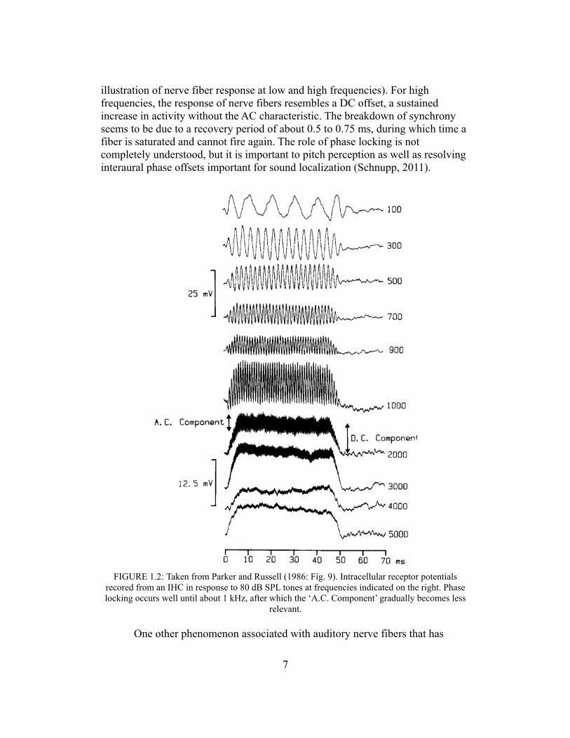
illustration of nerve fiber response at low and high frequencies). For high frequencies, the response of nerve fibers resembles a DC offset, a sustained increase in activity without the AC characteristic. The breakdown of synchrony seems to be due to a recovery period of about 0.5 to 0.75 ms, during which time a fiber is saturated and cannot fire again. The role of phase locking is not completely understood, but it is important to pitch perception as well as resolving interaural phase offsets important for sound localization (Schnupp, 2011).

FIGURE 1.2: Taken from Parker and Russell (1986: Fig. 9). Intracellular receptor potentials recored from an IHC in response to 80 dB SPL tones at frequencies indicated on the right. Phase locking occurs well until about 1 kHz, after which the ‘A.C. Component’ gradually becomes less

relevant.

One other phenomenon associated with auditory nerve fibers that has

7

potential importance for speech is short-term adaptation. For the first 20 to 30 ms following the onset of stimulus, the spike rate of a nerve fiber drops markedly from its level at the onset. Even after offset, this suppression is felt in the short-term reduction of firing rate even below the spontaneous rate. (Note that this type of adaptation also sets in for a tone when a sound masking that tone is removed.) Sound onsets are more salient than offsets in the periphery, and the neuron is more responsive to changes in input than to a continuous input (Gold et al., 2011).

Implications for speech

Peripheral processing might accentuate or diminish certain cues in speech. Bladon (1986) and Wright (2001, 2004) make the case that tendencies in linguistic sound systems and in historical sound change may have specifically auditory explanations (as opposed to acoustic ones). With regard to the questions addressed in this dissertation, the spectral effects of processing are going to be most important to consider. Bladon notes that the ‘analysis of spectral shape’ and ‘detection of spectral change’ (1986:4) occur in parallel; the former is directly relevant to the experiments in Chapters 3, 4, and 6.

The detection of spectral shape is key for making sense of many nonspeech results, and auditory critical bands make certain predictions about how speech spectra will actually be processed by listeners. Vowels and other sonorants can be described and identified by their formant structure (Peterson & Barney, 1952), which arises from the resonances induced by specific vocal tract configurations (Fant, 1970). These descriptions continue to be omnipresent in phonetics research. For the purposes of perception, formants contribute to the spectral shape that is processed by the ear. As will be discussed in detail later, however, formants cannot always be reliably analyzed by the auditory system (or, indeed, by signal processing algorithms); Chistovich and Lublinskaya (1979) identify a critical range of at least 3 Bark, well larger than the critical bands relevant to masking, within which formants seem to cohere for the purposes of phonetic identification. This finding has dramatic implications, which are discussed further in Chapter 5, for how listeners process spectral features and how formants interact with an auditory spectrum.

Central audition

As with the auditory periphery, I offer a brief description here of how the central auditory system transforms the auditory signal and some of its implications. Higher levels of the system begin to respond to more complex features in the stimulus, and the nature of these responses determines how acoustic cues from speech are ultimately represented.

The central portion of the auditory system relays neural responses from cochlear nerve fibers through the brain stem and ultimately to cortex. Along the

8

way, inputs are analyzed for pitch and temporal information, location, and other features. Higher-level processing and resolution of spectral and temporal information occurs at this stage. My review here will cover up to primary auditory cortex (A1) and will mostly not consider higher levels of processing. The central auditory system is staggeringly complex and still not well understood; considering this, my review here is shorter and more speculative in nature than for the peripheral system.

The first destination for auditory nerve fibers leaving the cochlea is the cochlear nucleus, a part of the brainstem. Nerves entering the cochlear nucleus are bifurcated, proceeding either through the dorsal or ventral cochlear nucleus—the former apparently more tuned to detecting spectral contrasts, and the latter to temporal processing (Schnupp, 2011). Ascending in parallel further up the brainstem, the paths eventually reach A1. In the brainstem we see the beginnings of significant qualitative deviations between the acoustic and the auditory. Several nerve cells in these stages do not perfectly preserve the output of auditory nerve fibers; rather, they aggregate responses from a number of convergent fibers into a different kind of signal altogether. Throughout the central auditory system, temporal aspects of the signal are transformed: the temporal syncing common to nerve fibers is replaced in many cases by the encoding of firing rate, without actually firing in time with a stimulus; some temporal resolution is lost, but we see the roots of parsing of the sound signal into temporal events (Pasley et al., 2012, Wang et al., 2008). Note that at cortex, phase-locked neurons respond at a rate well under 100 Hz (Wang et al., 2008), compared to reliable phase-locking under 1 kHz in the cochlea. A number of other relatively basic perceptual functions are also carried out by the brainstem, including pitch detection, localization, and even reflexive eye and head movements towards a sound source (Schnupp, 2011).

The re-encoding of temporal information at these stages is part of what appears to be a broader push away from the low-level peripheral signal and towards more ‘information-rich features of speech’ and of other auditory events (Pasley et al., 2012:9). The system has collected its raw data in the periphery and is now beginning to sort through and make sense of it. Analogy has been drawn between auditory and visual cortex, which is responsible for the detection of visual features—shapes, lines, movement—in the same way A1 is thought to be responsible for pattern detection in hearing (Moore, 2012).

Cortical structures themselves respond to a wide array of inputs including spectral modulation of various rates, onsets or offsets, spatial location, and even spectrotemporal responses that are so finely detailed they seem as if engineered for one specific purpose (Moore, 2012). Different spectrotemporal detection patterns can be characterized by spectrotemporal receptive fields (STRFs), which have also been utilized for some time (in a ‘spatial’ flavor) for the visual system. Many neurons respond only to very specific types of input, which can be estimated fairly well with STRFs. Tonotopy is preserved even in A1, where

9

several tonotopic gradients have been mapped (Talavage et al. 2004). Processes of spatial localization also remain very much active and complex at the cortical level, where it is estimated that over half of all auditory neurons are ‘preferentially or specifically sensitive’ to a sound’s location (Moore, 2012; see also Brugge & Merzenich [1973] for primate data).

A particularly promising area of recent neuroscientific research has been in the reconstruction of acoustics and phonetics from cortical responses to an auditory stimulus. Though a representation of cortical activation with high enough temporal and spatial fidelity is difficult to obtain, there have been some notable successes in this area. Mesgarani et al. (2008) showed that the multidimensional variability of A1 activation in ferrets can be used to recover many phones of American English. Furthermore, the authors show that a simple classification algorithm makes identification errors similar to those of human listeners. These results suggest that all the information needed to distinguish the important acoustic characteristics for speech sounds is present in auditory areas, without the need for a specifically phonetic layer (indeed, ferrets would have none), and that perceived similarity or confusability of phones also has a pure auditory basis.

A similar finding with human subjects comes from Pasley et al. (2012). In this study, electrocorticographic recordings of human cortex were made in response to isolated spoken words or sentences. Entire words were identified by a rudimentary speech recognition algorithm off of the reconstruction of either an auditory spectrogram or of spectrotemporal modulation. Recordings in this study were made in nonprimary auditory areas in the superior temporal gyrus, an intermediate area in the hierarchical processing of auditory stimuli. Responses at this stage still contained a large amount of acoustic detail—although it is unclear if enough spectrotemporal detail remains to reconstruct a human-intelligible sound signal—and were still sensitive to small acoustic variations. It is apparent from their results that sufficiently complex representations of sound exist in auditory cortex to support the phonetic details necessary to distinguish contrasts important to language as well as the characteristic modulations necessary for recognition of spoken words.

These results suggest that richly nuanced, non-auditory phonetic processing is not strictly necessary to classify speech sounds, although it certainly does not rule out the possibility of this layer in humans. Indeed, evidence exists from recent human imaging studies that some degree of organization aligning with phonetic features exists at levels of higher-order auditory processing (Mesgarani et al., 2014).

Sensitivity to spectrotemporal modulation

Another critical finding from Pasley et al. (2012) is that a nonlinear model of spectotemporal modulation (Chi et al., 2005) gave significantly better results than a linear auditory spectrogram reconstruction model, as the former captures

10

rapid modulations that are critical to speech intelligibility. The composition of auditory signals as modulations in the time–frequency domain is an important principle in neuroscience (Chi et al., 2001; Elliott & Theunissen, 2009; also Liu & Eddins, 2008), and phonetic classification can be approached through the consideration not of specifically identified acoustic features but of time–frequency STRFs in auditory cortex (Thomas et al., 2010).

Although there is ample evidence for spectrotemporal modulation being critical to and descriptive of speech perception, the cases under investigation in this thesis often do not need a full spectrotemporal account. This is most likely due to the nature of the stimuli under investigation. Many of the types of nonspeech referenced in Chapter 2 and studied further in Chapters 3 and 4 are fairly temporally static or have modulations gradual enough that they can be effectively accounted for as a sequence of spectral states. The speech representations of these sounds are generally vocalic in nature, with transitions mild enough that they remain representable in terms of distinct vocalic targets.

Some exceptions do exist and are discussed in the next chapter: specifically, those nonspeech sounds that are considered intelligible, possessing identifiable linguistic elements in words and syntax. A spectrotemporal model of speech perception (e.g., Chi et al., 2005) would be relevant for assessing these, and this may serve as a unifying account for the intelligibility of very acoustically different types of nonspeech. The focus of the original experimental work in this dissertation, however, is on shorter sounds that, while having phonetic relevance, are not linguistically complex. For such sounds, the spectrum is essentially the only source of information; spectrotemporal modulation and linguistic (lexical, phonotactic) information do not enhance their perception.

The nonspeech-related findings and intuitions gleaned from this project are, I think, extensible to a more generally spectrotemporal view of perception. This extension could account for other possible speech-nonspeech effects—for example, the associability of nonspeech transients with stop consonants, or other speech sounds that involve rapid spectral change (such as [l] in fluent speech). I do not claim that a spectral account without a consideration of speech as a time–frequency phenomenon can adequately explain speech perception; however, the ability of listeners to hear clear and stable phonetic categories from steady-state sounds does mean that a model must at least address spectra without a temporal component. Ultimately, a synthesis of spectrotemporal modeling and my ideas on spectral recognition are a likely avenue for accounting for more linguistically rich nonspeech.

Cue combinativity

How does sensitivity to various types of auditory events eventually yield truly phonetic percepts (that is, speech sounds or details of them)? Some findings and perspectives from auditory neuroscience suggest a bottom-up processing of

11

speech cues from primitive auditory objects: neural equivalents of logical AND and OR gates permit sensitivity to combinations of inputs or allow pooling that supports categorical perception, respectively. Strong support for this view comes from DeWitt and Rauschecker (2012), who perform a meta-analysis on a number of neuroimaging studies at various stages of linguistic processing and find clear hierarchical organization for the construction of complex auditory objects. Combination sensitivity in cortical circuits can be linked conceptually to cue combination sensitivity; that is, support for the cortical hierarchical processing of auditory objects is reminiscent of and perhaps compatible with an understanding of speech perception in which auditory cues combine in a logical network to give rise to phonetic percepts. The features themselves can be perceived independently and prior to categorization, while combination sensitivity links them together. A famous example of such a model for speech perception comes from Oden and Massaro (1978). (That said, the existence of a clear hierarchical progression at the cortical level may or may not offer support for a feature-combinatorial model at the psychological level.)

This notion of cue combinativity as a driver of phonetic perception supports a bottom-up, passive process in which cues aggregate until sufficient information for classification is reached. This contrasts with a top-down, analysis-by-synthesis (or Bayesian-like) approach, in which multiple hypotheses are tested for best fit with observed data (Poeppel, Isardi, Wassenhove, 2008). This promises to be an interesting perspective to consider for nonspeech sounds, some of which might contain incomplete sets of speech cues; should the sounds be judged perceptually by their gross similarity to speech sounds, or by their constituent cues?

Major theories of speech perception

Up until now, this review has concerned aspects of the auditory system that are key to understanding how speech sounds and cues to those sounds would be processed. At this point, I turn to post-psychoacoustic theories of speech perception—that is, those which address how a listener arrives at phonetic representations of speech from given auditory inputs. All of the experimental work presented in this dissertation has implications for theories of speech perception, which are discussed along with the experiments. The background here serves as a primer for those discussions.

Two reviews of speech perception by Diehl, Lotto, and Holt (2004) and by Fowler and Magnuson (2012) provide an overview of key phenomena in speech perception as well as of major schools of theory in accounting for these phenomena. Both reviews draw a broad distinction between general auditory and gesture-based theories. Stated briefly, the former school considers phonetic perception to occur through mechanisms common to auditory perception. Under this approach, even effects and phenomena that seem special to speech are

12

understandable through auditory abilities. Listeners need no inherent specialization for speech to perceive it. Support for a general auditory account of speech perception comes from many domains: for example, categorical perception has been shown to have an auditory basis, such as with common contrasts in voice onset time (Miller et al., 1976; although note Kewley-Port et al.’s [1988] rebuttal); and phonetic identification is responsive to acoustic context (Lotto & Kluender, 1998), even on the scale of seconds (Holt, 2005). Particularly compelling support comes from studies with nonhuman animals, such as chinchillas (Kuhl & Miller, 1975) and Japanese quail (Lotto et al., 1997), trained to recognize speech sounds. These animals, certainly lacking an evolved specialization for speech, can nevertheless interpret important speech contrasts.

Although general auditory abilities can account for many speech phenomena, other evidence suggests that listeners’ understanding of a speaker’s articulatory gestures inform how they perceive the signal. Speech acoustics are famously difficult in the sense that a single articulation will have quite different acoustic consequences given different phonetic contexts (the ‘lack of invariance problem’), although perceptual systems sort out this inconsistency effortlessly. There is also the matter of how listeners account for coarticulation: although many context effects have been presented in support of an auditory contrast explanation, others seem not to have any clear auditory account, relying instead on listeners understanding articulatory mechanics (Mann & Repp, 1980; Fowler, 2006; Viswanathan et al., 2010). The importance of visual information to speech also supports the recruitment of articulatory knowledge, as listeners will reject auditory hypotheses that are wholly inconsistent with visual evidence (McGurk & MacDonald, 1976).

An early framework for explaining a perceptual parity between articulation and acoustics is the motor theory of speech perception (Liberman et al., 1967; Liberman & Mattingly, 1985). Under this view, basic constituents of perception are the speaker’s intended gestures, which are direct consequences of invariant motor programs for moving speech articulators. The motor theory easily deals with the lack of invariance problem by automatically assigning a motor action, which is linkable directly to distinctive features of speech sounds, to all of its possible acoustic realizations. The actual linkage between these motor programs and their acoustic consequences owes to a hypothesized specialization for speech with an innate mapping between them (although this can be tuned during first language acquisition). It is primarily for this reason that a strong version of the theory—i.e., that phonetic parsing depends on motor knowledge or ability—is not well supported by neuroimaging evidence. Current understanding is that sensory-motor integration, in which motor circuits are activated in response to speech and other sensory inputs, is almost certainly not critical to speech recognition, although top-down influences on heard speech are not discounted (Hickok, 2009).

The other most influential theory of speech perception as gesture

13

perception is direct realism. Fowler (1986) adapts to speech an event-theoretic framework from, among others, Gibson (1966/1982, 1979). Under this view, speech articulations are perceived directly, through whatever sensory modalities are available, as would be the acoustics of any other natural system. Crucially, perception does not require a specialization for speech, but rather depends on normal event- and source-perceiving mechanisms. This latter point goes at least partway towards explaining nonhuman speech perception and is reinforced by experiments demonstrating qualitative similarities between perceiving speech and perceiving other auditory events with a clear mechanical source (Fowler, 1990; Fowler & Rosemblum, 1990). Direct realists differ as to how the system is tuned through learning (Fowler, 1986; Best, 1995) but generally agree on the core of the theory that sound-producing events constitute the basic objects of phonetic perception.

‘Speech mode’

Even if speech and other auditory stimuli are processed on common hardware, the question remains open as to whether there are ‘software’ differences—i.e., distinct processing strategies that are typically engaged for speech and not for nonspeech. Numerous aspects of speech perception that do not have a clear basis in auditory psychophysics have been catalogued. Some of these phenomena, such as phonetic context effects and audiovisual integration, have been discussed already. Others evidence includes trading relations, in which a phonetic percept can be preserved, even when altering a critical cue, by changing another cue to compensate (Repp, 1982). In this way, listeners are less sensitive to acoustic variations, even those that are normally phonetically detectable, when such variations do not lead to a change in phonetic identity. (Even more generally, categorical perception of speech sounds demonstrates an insensitivity to acoustic changes that otherwise would be psychophysically detectable.) These phenomena do suggest that phonetically specialized processes enter into perception, even at a low level.

Clearer evidence of a distinct mode for speech perception comes from experimental work in which the same stimulus elicits different responses based on the listener’s expectation. One way in which this is possible is to exploit duplex perception, in which a certain auditory stimulus is heard both as its own event and as a part of the spectrum of a speech sound. For example, Mann and Liberman (1983) demonstrate a case of duplex perception in which a third-formant transition, presented dichotically with a speech syllable, both triggers a shift in perceived stop identity ([d] to [g]) and is heard as a simultaneous chirp. Discrimination of two trials featuring transitions with different starting frequency differs based on whether listeners are instructed to attend to the speech or nonspeech ‘side’ of the duplex percept: discrimination of phonetic identity is enhanced across the categorical [d~g] boundary, while discrimination of chirp

14

frequency is not.A direct comparison of speech and nonspeech is also possible using sine

wave speech (SWS) stimuli. Using these stimuli, possibly confounding pure acoustic differences between speech and nonspeech tokens are eliminated. Evidence for distinct speech and nonspeech modes of listening to SWS come from multimodal studies that show that listeners integrate audiovisual information (Tuomainen et al., 2005) and modulate phonetic category boundaries (Vroomen & Baart, 2009) only when listening in a speech mode. Neuroimaging evidence also suggests the recruitment of different circuitry when considering a stimulus as speech rather than nonspeech: cortical activation differs depending on whether a listener is primed to hear SWS as speech (Liebenthal et al., 2003; Dehaene-Lambertz et al., 2005; Möttönen et al., 2006).

The assignment of speech-specific processes to a perceptual mode rather than an entirely different system or module raises the question of how this mode is triggered. Furthermore, it allows for the possibility that the mode can be active to a partial degree—or always active even when a speech source is not present. The implications of a speech mode for nonspeech listening will be discussed further in Chapter 2.

Conclusion

More detailed coverage of auditory physiology, psychoacoustics, and the theory surrounding speech perception is certainly possible; this review has covered only some of the essentials. To address and discuss the major questions of this dissertation, some background in all of these areas was necessary. The behavioral experiments to come have clear implications for speech perception theory, and the study of spectral perception later on owes much to the modeling of auditory periphery and deals with many issues that are informed by more recent understanding of the central auditory system. The discussion spectral processing also deals extensively with questions of physiological plausibility, and an inclusive (even if somewhat shallow) picture of the auditory system is useful for reflecting on those questions.

At this point, I turn specifically towards the ability to hear, understand, and classify nonspeech sounds as speech. Chapter 2 provides a literature review of studies that have demonstrated this type of perception.

15

Chapter 2Speech-nonspeech perception

Most of the original experimental work in this dissertation asks listeners to make phonetic judgments on nonspeech sounds. This method fall into a rich history of similar work. This chapter is a review of experiments on what I term ‘speech-nonspeech’ stimuli: sounds that are clearly not speech but have a tendency, inherent to their acoustics, to be identified as certain speech sounds. Similarly, the term ‘speech-nonspeech perception’ refers to hearing phonetic details in nonspeech. I also address related studies in speech perception that demonstrate the effect of nonspeech on nearby speech—although these cases may not feature overt judgments on nonspeech, they do leave open the possibility that nonspeech context sounds are influencing speech judgments. To begin, I present some of the motivations for using speech-nonspeech methods to study ordinary speech perception and elaborate on what is entailed by speech-nonspeech perception.

Why nonspeech?

There are a number of reasons to consider data from speech-nonspeech conditions for the perception of natural speech, especially at a low level. Several theoretical questions can be directly addressed using such stimuli, which can be designed with much more freedom than natural speech. These questions range from broad ones that define the field—e.g., to what degree speech is ‘special’, and under what conditions—to specific questions of how the system works—e.g., the translation between an auditory representation of a speech signal and the hierarchical beginnings of a linguistic representation. Even with an eye towards application, speech-nonspeech perception can inform our understanding of speech perception in non-ideal listening environments, which is a major difficulty for hearing-impaired listeners and for automated systems.

By their very nature, speech-nonspeech tasks exploit the differences between auditory perception and phonetic/linguistic perception. Even where speech processing can be argued to rely on general auditory mechanisms, a speech judgment will often require some kind of categorical decision in terms of linguistic categories. As noted in the previous chapter, many theoretical approaches to speech perception posit the action of processes apart from audition (even if these processes are driven by other general cognitive abilities, as with direct realism). As this is still an active area of debate, the implications of speech-nonspeech results for major theories of speech and auditory perception should be considered.

Apart from addressing broader theoretical questions, exploiting speech-nonspeech phenomena also allows us to examine more detailed aspects of

16

perception. By carefully designing nonspeech stimuli and presentation conditions, it is possible to observe the results of speech perception given a wide variety of inputs. In a sense, the system can be reverse-engineered by examining its responses to these atypical inputs. Faithful models of human perception should generate accurate predictions of speech and nonspeech inputs alike. One avenue of approach from earlier work has been to generate stimuli that contain putatively necessary speech cues without other speech characteristics.

In the sections below I review several types of stimuli and conditions that fit my definition of speech-nonspeech research. It is a diverse body of work, both in the types of stimuli used and the types of evidence relied upon to demonstrate speech-nonspeech processing: intelligibility of nonspeech, matching of nonspeech to speech categories, and even the impact of language experience and phonological constraints upon auditory perception. Some of these sounds are quite similar to speech, others much more alien. All are identifiable as nonspeech, and for all of them there is some type of evidence that they are being processed in a way at least partially directed by speech perception.

Single-resonance harmonic complexes

Convincing approximations of natural speech can be created by carefully tuning parameters of a speech synthesizer. The traditional source-filter signal flow of most speech synthesis allows for exact control over variables that are directly relatable to speech production, and therefore measurable. Even when synthesis is coarsely modeled on acoustics or production, with noticeable divergences from a natural utterance, the result will usually be strongly evocative of a human voice. For the purposes of this review, I consider any sounds synthesized with appropriately detailed parameter settings to qualify as legitimate speech sounds, even if they have a slightly synthetic quality, because there is essentially no disagreement between listeners as to their phonetic interpretations. Inconsistencies in the perceptual nature of natural speech and synthetic speech generated by rule have been noted (Pisoni et al., 1985); however, for adult listeners in noise-free environments, the cost to intelligibility for synthetic speech is minimized (Logan et al., 1987). As most of the studies considered in this chapter are conducted under idealized laboratory conditions, synthetic speech will be considered ‘close enough’ to natural speech and, more importantly, categorically different from obviously nonspeech sounds.

For experiment designers, synthesis also offers a means of generating near-speech sounds by setting certain parameters to unrealistic values, enough to distort the speech percept while preserving several other characteristics of the signal. The simplest example of this type of manipulation is the removal of formants by using a reduced number of the synthesizer’s resonators. The result is a sound that contains many acoustic markers of speech but, given the nature of its spectral envelope, is in no danger of being mistaken for speech. Because two

17

formants are generally sufficient for vowel recognition (Peterson & Barney, 1952; Cooper et al., 1952), it is usually necessary to eliminate all but one resonance to generate a decidedly nonspeech sound. With only a single spectral peak, cases of duplex perception are possible for these types of stimuli: some listeners describe these sounds as a buzz with a concurrent chirp (at the resonance’s frequency), while this chirp also determines the timbre of the sound (Remez et al., 2001; Finley, 2012; see also Fowler & Rosenblum, 1990).

Some early investigations of speech-nonspeech processing came out of attempts to recreate vowels using only a single resonance. Delattre et al. (1952) attempt to classify a number of outputs from a speech synthesizer set for one formant. Miller (1953) reports also on vowel identifications for many settings of a two-formant synthesizer, including values for which the formants are set to be identical (up to 1.2 kHz). A single low formant leads to identifications as a mid or high back vowel, whereas a formant at or above 800 Hz is identified as a lower back vowel (English [!] or ["]). At high values, above 2160 Hz, sounds became front vowels—first [#], then [e], then [i]. For the higher values, the single formant seems best matched to the F2 of the evoked vowel, whereas for lower values it seems closer to an average of the first two formants.

The observations by these authors have led them and others (e.g.: Assmann, 1991; Chistovich & Lublinskaya, 1979; Crowder & Repp, 1984) to speculate as to the nature of formant recognition by the auditory system. There are a variety of suggestions for dealing with what appear to be different classification strategies when two formants can be separately resolved (some of which will be revisited in Chapter 5); what can be said for certain is that a naïve model of the first two formant frequencies fails to account for the SFS observations. The use of non-canonical speech sounds as experimental stimuli elucidates these shortcomings. The experiments in Chapter 3 use as stimuli, among other sounds, single-formant vowels generated using the Klatt (1980) speech synthesizer. As will be seen, some of these artificial vowels have demonstrable phonetic value.

Apart from its potential in speech-nonspeech experiments, single-formant speech (SFS) or acoustically similar sounds have seen use in other research applications, such as the measurement of JNDs in formant frequency (e.g., Lyzenga & Horst, 1995), measurement of auditory nerve fiber activity (Delgutte, 1980), or the detectability of signal processing artifacts (Kortekaas & Kohlrausch, 1996). These studies do not ask for phonetic judgments of the stimuli, although it is a fair question whether the ability of a single-formant vowel to evoke speech has implications for their results.

Sine wave speech

Given the ability to selectively remove acoustic features from speech, synthesizer nonspeech is a useful tool for gauging the importance of assumed speech cues. For sine wave speech (SWS), a variety of nonspeech that has been

18

used extensively, a typical spectral profile is not present; however, the intuition at the heart of generating these types of stimuli is that at least some of the essential cues for recognition are (or are determined by) speech formants. For these sounds, frequency modulated (FM) pure tones are synthesized at frequencies and amplitudes derived from formants following acoustic analysis. In most cases, the first three formants are used.

Remez et al. (1981) perform the first perceptual investigation of sine wave analogues of speech, finding some intelligibility of SWS utterances when the first two or three formants are present. Other combinations of one or two of the three lowest formants yield essentially no intelligibility. The authors conclude that ‘traditional formant-based acoustic cues’ are absent, but the ‘pattern of change in the natural signal’ is preserved enough to allow for some intelligibility (949). Their accounting for the results implies that the tones themselves do not serve as spectral determinants or cues as formants do, but that changes in tones are faithful enough representations of formant transition cues. (A strong version of this claim for SWS is incompatible with some of the work performed and referenced in Chapter 6.)

A hallmark feature of SWS is its fragile status as speech. Although some listeners hear speech immediately, most do not, and experimenters have devised a number of strategies to modulate the speech status of SWS within an experiment. As such, it makes a useful tool for identifying differences between putatively distinct modes of processing for speech and for general sounds (Vroomen and Baart, 2009; Liebenthal et al., 2005). Whether or not SWS is heard as speech also affects whether listeners can hear differences requiring the integration of phonetically associated simultaneous cues (Best et al., 1981).

As with SFS, SWS contains elements that are heard both as components of the spectrum and as individual events. Whereas with broadband, natural speech, listeners assign the entire signal to a single stream, these less spectrally dense stimuli show evidence for parallel processing of sound for different outputs. Remez and Rubin (1993) show that the first formant is both interpreted for its contribution to the speech-nonspeech spectrum and considered by most listeners to represent the intonation contour of the sentence. Similarly, Remez et al. (2001) assert that SWS is ‘bistable’ in terms of two concurrent modes of perception and show that listeners can resolve constituent tones from a three-tone complex in a way they cannot with speech and formants.

The general pattern of results from SWS—i.e, that it is intelligible—seems to support the notion that formant modulations are sufficient or possibly fundamental cues for spectral recognition. However, these results have the potential interpretation that the constituent tones act to shape the spectrum, which is identified by other means, rather than acting as discrete cues in their own right (Hillenbrand et al., 2011).

19

Pure tones and filtered speech

Evidence that SWS can be perceived as speech is its intelligibility. This is particularly strong evidence, and for other types of sounds this may not be possible. One such case is with single tones, which could be seen to constitute a partial SWS signal. There has been no demonstration of intelligible fluent speech drawn from a single tone (although note that Saldaña et al. [1996] show that a paired F2 analogue can increase intelligibility of visual speech). Nevertheless, there is evidence that single tones evoke certain vowel sounds for listeners, a phenomenon that I refer to in this dissertation as Vokalcharakter, following the designation by Köhler (1910). Some prominent investigations of this phenomenon are by Farnsworth (1937), Fant (1973), and Kuhl et al. (1990). The general pattern of identification is similar to that found with SFS by Delattre et al. (1952) and Miller (1953): low tones are readily identified as mid and high back vowels, midrange tones with low back vowels, and higher tones as high front vowels, with other vowels only weakly represented.

Another type of stimulus that should be discussed alongside pure tones is filtered speech. The similarities between these may not be immediately evident. However, they are theoretically identical in the sense that any band-pass filtered complex sound will, with the narrowing of the passband, approach a pure tone. If the Vokalcharakter phenomenon is a case of ordinary spectral perception and categorization, then filtered speech and tones should be identified similarly. Early studies of filtered vowels (Lehiste & Peterson, 1959; Chiba & Kajiyama, 1958) find response patterns similar to tonal Vokalcharakter and SFS: high-pass filtered vowels become high front, low-pass high back, and band-pass low back (in the mid-frequency range). A comprehensive historical review of the study of tonal Vokalcharakter and of filtered vowels is given in the introduction to Chapter 4, ‘Tone-evoked vowels and semivowels’.

It should also be noted that I distinguish between speech or vowels that are very narrowly filtered, to the point of changing the phonetic identity of the sound, and speech that is filtered to the point of reduced intelligibility. There is a long history of research performed on the intelligibility of band-limited speech, for both psychological research and engineering purposes (see: Allen, 1994; Cunningham, 2003). However, these sounds are not exactly ‘speech-nonspeech’ because they are generally not filtered so aggressively to become unidentifiable as speech. Additionally, they are much more plausible as real-world stimuli, as the filtering could conceivably be a simulation of a noisy channel or a real-world acoustic setting (e.g., a talker on the other side of a wall).

Noise-vocoded speech

An entirely different type of nonspeech is found in noise-vocoded speech (NVS). The procedure for generating these sounds is to extract temporal

20

amplitude envelopes of frequency bands (usually very broad) and apply these to noise in the same bands. The result is an artificial sound with near-perfect intelligibility with as few as three or four bands. Even isolated consonants and vowels are highly intelligible, with manner and voicing of consonants easily detectable at only two bands (Shannon et al., 1995). Impressionistically, NVS resembles a harsh whisper; indeed, in acoustic terms, the stimulus is a broadband noise source similar to glottal frication with the application of a very temporally faithful dynamic filter.

As is definitely the case for single-band NVS, and still true of multi-band NVS, temporal cues are preserved while spectral ones are wiped out to some degree. Certain spectrotemporal cues, such as formant transitions, are lost entirely if they do not cross a band cutoff (Shannon et al., 1995). That said, the spectrum does provide key information for phonetic identity despite its coarse resolution. In a later study, Shannon et al. (1998) find that, although recognition is robust to changes in the cutoff frequencies of the bands, performance does decrease when there is a mismatch between the analysis and carrier bands. These stimuli are not intelligible merely through having several concurrent channels of temporal cues, but require a non-frequency-transformed representation of the spectrum.

Top-down processes also play a role driving the intelligibility of NVS sentences. Listeners improved for highly reduced NVS sentences when given lexical training for their content, suggesting that lexical and other top-down processes play a major role in disambiguating the cases of reduced spectral and phonetic information (Davis et al., 2005). The notion that complex learned processes are involved is also supported by a finding by Eisenberg et al. (2000): children ages 5-7, although beyond most phonetic stages of language acquisition, require higher spectral resolution to attain the same degree of intelligibility for NVS than do older children (ages 10-12) and adults.

Other studies have generated nonspeech in a similar manner using sine-wave carriers at the analysis band center frequencies rather than noise-band carriers (Hill et al., 1968; Dorman et al., 1997). These sounds will have the same key spectrotemporal maxima, but with a considerably more gapped spectrum. Despite these differences, Dorman et al. (1997) find NVS only slightly more intelligible than the sine carrier, whose perception may depend on the same abilities recruited when listening to speakers with widely spaced harmonics from a high F0.

Intelligible varieties of nonspeech have also been used in neuroimaging studies to map areas of the brain responsible for language (Scott et al. 2006 for NVS; Liebenthal et al., 2003, Möttönen et al., 2006 for SWS), as conditions of presentation can make a single acoustic input either intelligible or unintelligible. By controlling whether or not the sound is heard as speech, post-auditory processing stages specific to speech can be partially mapped.

21

Other evidence: context effects of nonspeech on speech

Similar types of work on speech perception have explored the effects of nonspeech context on the identification of speech targets. In these cases, phonetic judgments are not being made directly on the nonspeech sounds, but on ambiguous speech sounds whose classification is affected by nonspeech. I discuss these cases separately here because there is no clear evidence that the effects are driven by speech-nonspeech processing; they may be purely auditory in nature and require no intermediate phonetic step. Said another way, they operate according to predictions of general auditory models, and there is no evidence that speech or language abilities play a role. Auditory effects in these types of studies are generally contrastive in nature: phonetic identification relying on spectral energy that matches the frequency range of adjacent nonspeech will be dispreferred compared to when that context is not present.

Compensation for coarticulation is a condition that shows these effects quite clearly. Adapting Mann’s (1980) paradigm, Lotto and Kluender (1998) demonstrate a smaller but similar shift in identification boundary between /da/ and /ga/ when the preceding context is either steady or FM tones matched to the F3 offset of /al/ or /ar/. Holt et al. (2000), in a paradigm similar to Lindblom and Studdert-Kennedy’s (1967) speech study, show a boundary shift between two vowels differing in frontness based on flanking tones matched to the F2 transitions of surrounding stops /b/ or /d/. Using SFS, rather than tones, Crowder and Repp (1984) show a constrastive effect on vowel identification that persists whether the context is a fully synthesized high front vowel or a SFS token with a resonance at the F1 of that vowel.

To some degree, contrast effects like these can be explained through simple peripheral masking. Precursor tones near formant frequencies do induce some energetic masking on following speech sounds, as evidenced by a strengthened effect with increased tone amplitude and decreased gap duration (Fowler et al., 2000; Viswanathan et al., 2010; Viswanathan et al., 2013). However, the presence of masking as a partial explanation for some of these effects does not discount more central auditory contrast explanations. Holt (2005) extends the findings on contrast by demonstrating that nonspeech sounds affect speech categorization with as much as 1.3 seconds of intervening silence. Nonspeech sounds in Holt’s study were collections of short tones uniformly distributed over a given frequency range and played in random order. Identification of ambiguous /da/~/ga/ tokens was affected by the frequency distributions of the preceding nonspeech tones. The long time course of this effect precludes peripheral masking and may be related to auditory mechanisms that are also at the root of normalization processes (Holt 2006). Wade and Holt (2005) demonstrate an effect of pure tone on preceding stop identity (so long as the tone was not too close to the stop to be interpreted as part of its formant transitions), demonstrating that this type of contrast can operate in the reverse direction.

22

Additionally, contrast effects have been shown to operate even when target and context are presented dichotically (Holt & Lotto, 2002; Lotto et al., 2003). All three of these types of evidence challenge a purely peripheral account.

Similar studies have been performed with small children, further probing the question of whether innate or learned processes are responsible. Hufnagle et al. (2013) find that the stimuli of Holt (2005) elicit similar responses in five-year-old children. Indeed, even with pure speech stimuli, prelinguistic infants show a pattern of compensating for coarticulation (Fowler et al., 1990). In contrast, Kuhl et al. (1991) show that matching of a visual speech syllable to a pure tone is somewhat predictable (from known patterns of tonal Vokalcharakter) with adult listeners but not with infants. The lack of an effect in this case could be explained by the necessity of learning the associations between visible and audible speech, which is required for this paradigm. That is to say, the auditory associations between tone and speech may indeed be present for infants, if auditory vowel perception depends on innate auditory abilities, but they are unable to indicate this given their lack of experience with audiovisual integration of speech.

Other evidence: linguistically mediated nonspeech processing

Another type of evidence to consider as supplementary to speech-nonspeech effects is the linguistically or phonetically based processing of auditory stimuli. In these cases, although there is no speech judgment is being offered on the nonspeech, the linguistic experience of listeners in some way predicts how they will respond to nonspeech stimuli. One way to interpret these findings is that some amount of language specialization occurs at pre-linguistic auditory stages, in which case abilities tuned for speech perception are being applied to nonspeech, as they are in speech-nonspeech perception.

Prosody is an area where these effects have been most convincingly demonstrated. Speakers of tonal languages show a higher sensitivity to changes in pitch (Krishnan & Gandour, 2009). Differences in sonority constraints on syllabification between English and Russian leads their respective speakers to ‘syllabify’ nonspeech sounds into beats differently (Berent et al., 2010).

Segmental effects are somewhat more difficult to observe. Despite the inability of many native Japanese speakers to distinguish English /r/ and /l/, Miyawaki et al. (1975) find no effect of native language on perception of SFS modeling F3 of those sounds. Similarly, Iverson et al. (2011) find that Hindi speakers’ insensitivity to English /w/-/v/ contrast does not extend to most nonspeech sounds in which frequency, amplitude, and/or frication cues were removed from /w/ and /v/. They do, however, find a statistically reliable difference between English and Hindi speakers’ identification of a certain narrow class of nonspeech that maintained amplitude modulation and frication cues. They suggest that this is evidence for linguistic specialization in phonetic processing. From a speech-nonspeech perspective, either this narrow class of sounds serves as

23

an acceptable input to speech perception, or auditory processing follows strategies tuned for speech.

Discussion

The various types of speech-nonspeech sounds discussed in this chapter are remarkably eclectic, as are the types of evidence given that they are being processed as speech. That this processing can be demonstrated for such varied sounds is encouraging, as it highlights the robustness of speech perception under many circumstances. At the same time, this diversity puzzling, as it makes it difficult to say exactly what these sounds have in common that promotes speech-nonspeech processing. That said, comprehensive theoretical approaches to speech perception would not necessarily require any cues to be shared between different types of nonspeech. The interaction of bottom-up and top-down processes in perception is well known, and higher-level phonetic or linguistic knowledge can fill in missing lower-level cues (e.g., Ganong, 1980; Pitt & McQueen, 1998). So if, for example, SWS contains sufficient spectral cues, and NVS contains sufficient temporal cues (along with rudimentary spectral information), a model including a combination of bottom-up and top-down processes could predict the intelligibility of both even if disjoint cues are present, as long as there is enough phonetic information within each signal to activate higher-level representations.

Accounting for low-level speech-nonspeech effects, however, requires careful consideration of the mapping between an auditory percept and a phonetic one. For many stimuli, listeners lack temporal cues or linguistic information but are nevertheless able to classify nonspeech spectra into phonetic categories. Classification of isolated sounds does not depend on higher-level effects, either lexical in nature or owing to an understanding of articulation or phonotactics. Many of the types of nonspeech considered above hint that the overall shape of the spectrum is consistent between sounds that are identified as the same. I addressed three types of ‘peaky’ nonspeech: SFS, pure tones, and filtered vowels. For all of these, mappings between center frequency and vowel were conducted some time ago, prior to 1960, and are in strong agreement across all three types of stimulus—and this agreement concerns both the vowels evoked at each frequency and the strength of those associations. All types can also be caricatured as a generally low spectral envelope with a bump at center frequency; apparently, this caricature has some explanatory power in terms of how human listeners will classify the sounds. The nature of this modeling intuition will be elaborated upon in Chapters 4-6.

At a higher level, what do speech-nonspeech effects say about the relationship between speech and general auditory perception? Two alternatives could be argued: one, that the effects of speech processing owe entirely to auditory abilities, and that a speech treatment of nonspeech is the logical consequence of a listening system whose action is undifferentiated with respect to

24

its inputs; or two, that speech perception is to some degree specialized but permits nonspeech inputs for one reason or another. The first position is attractive in its parsimony, as it does not require answers to the questions of how and why the speech perception system admits nonspeech inputs, but in avoiding these questions it requires the espousal of a rather extreme auditory theory of speech perception. The second view, on the other hand, allows for a system that is flexible in its ability to consider articulatory and multi-modal information. Moreover, this view works effortlessly with the cases cited before in which differences in processing were noted when identical auditory stimuli did or did not enter into a ‘speech mode’.

Why might speech perception freely admit nonspeech inputs? Certainly, in many situations this would hurt intelligibility of speech in noise, as the latter could not be as effectively segregated to provide masking release. Probably more seriously, it would lead to spuriously interpreted speech cues in cases where spectrotemporally overlapping sound events were present. Indeed, cases of duplex perception (in which sounds concurrent with speech are heard both as a segregated sound and as a spectral cue for speech) show this very situation in unnatural conditions (Rand, 1974; Liberman et al., 1981). Another example comes from Wade and Holt (2005): although they note a contrastive effect of tone on preceding stop identification, removing the temporal gap between them produced an ‘assimilative’ effect in which spectral information of the tone is incorporated into the stop’s phonetic identity. That said, all of these cases are highly artificial experimental conditions, with judgments being asked on isolated tokens, and there is reason to believe that listeners do not make such errors in natural listening conditions. In real-world listening, speech inputs will have richer lexical information and other informative redundancies, and there will likely be substantial spatial release from sounds that would either mask or combine spuriously with speech. (Even dichotic presentation does not contain proper localization cues, thus impairing listeners’ ability to segregate them.)

On the other hand, allowing nonspeech admission to the speech system does have several advantages. Once again, ecological considerations come into play: listening conditions are hugely variable, and a system flexible to its inputs will be able to automatically process speech even when highly acoustically degraded. It is not necessary to define criteria for when a degraded speech signal is speechlike enough; sounds are automatically assessed as possible sources of speech, and there is no hard acoustic threshold past which listeners stop trying to understand it. Indeed, it is easier to imagine mistaking the sound of a creaky door for speech than failing to immediately recognize the sound of a human voice. To offer further speculation, speech-nonspeech processing, in the sense of speech listening that persists even after discounting a possible speech source, may even be a strategy for rehearsing and imitating the sounds of natural events.

Finally, some consideration is also due to the implications of speech-nonspeech for direct realism. At first blush, any readily accessible phonetic

25

content of obviously nonspeech sounds is problematic for direct realism because there is clearly no direct perception of any motor-acoustic event. Direct realism would predict that natural nonspeech sounds with a transparent source would be handled similarly to speech, whereas the response to unnatural sounds would be qualitatively different (Fowler & Magnuson, 2012). The matching of speech sounds to nonspeech, whatever the features determining their acoustic similarity, is decisively compatible with an auditory view of speech perception in which new inputs are matched to known prototypes.

Can the position that gestures are perceived directly for speech-nonspeech be somehow salvaged or repaired? This seems more a philosophical question than an empirical one. Best (1995) discusses the direct realist perspective on impoverished inputs and what inference would be necessary to resolve them. She claims that the assumption underpinning the empiricist tradition in psychology is that impoverished, indirect information about the world is gleaned from sensory organs and must be filled in through knowledge; alternatively, a direct realist perspective views a continuous flow of multimodal and proprioceptive input as a direct, coherent representation of the world. An experienced perceptual system, then, is attuned to ‘higher-order invariants available in the flow of stimulus information’ (175).

My interpretation of Best’s characterization of direct realism in its applicability to nonspeech is that nonspeech must possess these acoustic invariants in order to have any perceived phonetic associations. Furthermore, stimuli presented in a laboratory setting are usually deprived of reliable multimodal information. Under a direct realist view, then, sounds heard in these conditions are not made to sound like speech by simply being matched to the closest known speech sound category, but are parsed by their hallmark features into perceived events. These sounds must therefore contain some features central to speech, not just similar to it; if anything, direct realism predicts that speech-nonspeech perception is a strong strategy for determining indispensable acoustic features for speech.

Work to be done

The observation noted above that nonspeech can affect categorization of nearby speech is potential evidence for speech-nonspeech processing of those sounds. I gave several examples of context effects of nonspeech sounds on speech. However, it is unclear whether speech-nonspeech processing is truly involved because the effects can, so far, be explained on purely auditory grounds through masking and central auditory contrast effects. Better evidence would be a context effect that is driven by nonspeech in an unambiguously phonetic capacity, as opposed to an auditory one. The experimental work in the following chapter addresses this gap in the literature by showing effects of this type.

Of all the types of stimuli for which speech-nonspeech processing has

26

been observed, the weakest effect is arguably with pure tone Vokalcharakter. That tones are in fact triggering speech processing via spectral similarity to certain vowels, rather than some other mechanism, is fairly well supported by comparison with the perception of filtered vowels. Nevertheless, the link between vowels and tones is still rather tenuous, and it would help to have better evidence that Vokalcharakter depends on the same mechanisms as normal speech perception. Chapter 4 presents an experiment that extends Vokalcharakter to dynamic contexts that bolster the case for its speech-nonspeech nature by showing the effect at rates of spectrotemporal modulation similar to those of speech.

Finally, the evidence for speech-nonspeech processing also suggests the importance of considering speech perception in its ecological context. Most targeted experimental research does not attempt to recreate natural listening environments for the stimuli; even those that test listening under difficult conditions usually do so by the addition of broadband noise or by processing the signal in other ways that are easy to quantify but hard to find in nature. Although speech-nonspeech tasks are fundamentally unnatural, the phonetic value of these sounds suggests a recognition system that is exceptionally robust to interference (as we know also from real-world performance that it must be). It may be that the system’s efforts to hear speech from laboratory nonspeech stem from the same mechanisms that allow for the robust intelligibility of speech in suboptimal conditions. Research directly comparing speech-nonspeech listening and real-world degraded speech listening is needed to determine if this is the case.

Even with what currently exists, however, there are many types of evidence that suggest the action of ordinary speech perception processes at work when listening to certain nonspeech sounds. Part II is my further contribution further to this body of experimental literature; in Part III, I work from the findings of my experiments and others to investigate the nature of spectral processing in human listeners.

27

Part IIBehavioral experiments

28

Chapter 3Speech-nonspeech in compensation for coarticulation

In the previous chapter I introduced several cases in which nonspeech was shown to have a context effect on the classification of adjacent speech sounds. Compensation for coarticulation, which in some sense involves the perceptual disentanglement of a speaker’s coarticulated gestures, was demonstrated for nonspeech sounds, which presumably have no articulatory properties for human listeners. These studies usually offered some alternative explanation for the effect through some combination of peripheral and central masking and contrast mechanisms. As such, there was no clear evidence that speech-nonspeech processing of the stimuli was relevant to the context effects. In this chapter, I present a series of experiments that show compensation to nonspeech coarticulation in a condition that does rely on speech-nonspeech processing, suggesting that speech-nonspeech processing happens at early, preattentive stages of perception.

Compensation for coarticulation is a robust phenomenon and has been tested under a variety of different conditions (e.g., stop identification: Mann, 1980; Lindblom & Studdert-Kennedy, 1967; F0 and vowel: Silverman, 1987), with variety in the taxonomic species of the listener, and with a variety of different explanations. In many cases, a gestural explanation is difficult to disentangle from a contrast explanation, as spatially similar configurations of articulators usually give rise to similar acoustic outputs. Targeted studies have shown evidence both for pure auditory phenomena, such as masking and spectral contrast, and for event-based disentangling of articulation to recover the speaker’s intended speech sounds. Examples of the former include artificial setups such as tonal or other nonspeech contexts, or contexts produced by opposite-gender speakers from the targets (Lotto & Kluender, 1998; Holt et al., 2000; Lotto et al., 2003); the latter, cases in which listeners compensate properly for coarticulation, but contexts do not have spectral overlap with targets that would predict contrast effects (Fowler, 2006; Viswanathan et al., 2010; Johnson, 2011). Effects that are apparently compensatory with nonspeech contexts has also been observed, as was discussed in Chapter 2.

The condition explored in the present chapter is anticipatory lip rounding on English [s] before rounded vowels, similar to the task by Mann and Repp (1980). Lip rounding on [s] lowers its spectral mean (Soli, 1981), making it acoustically closer to [$]. Though English [s] and [$] differ in a number of acoustic dimensions, the most salient of these is in spectral mean (Li et al., 2009). When before rounded vowels, then, listeners expect to hear a lower-frequency [s] than before unrounded vowels; hearing an ambiguous sound somewhere between the two, they would be more likely to perceive it as /s/ before a rounded vowel than

29

unrounded, attributing the lower-than-usual centroid to rounding coarticulation. Additionally, the high front vowel [i] features a labial configuration that creates the opposite effect on the fricative, and this effect is noticed by listeners (Yeni–Komshian & Soli, 1980). By exploiting coarticulatory effects of more rounding and of less rounding, the measurable difference between vowel contexts can be maximized.

I took a cue-based approach to determining the best way to design nonspeech stimuli to mimic front unrounded and back rounded vowels for English-speaking listeners. Because all front vowels in English are unrounded and all back non-low vowels rounded, the roundedness of any given non-low English vowel can effectively be determined by its backness, which is measurable in its F2. Furthermore, because rounding lowers F2, a very high F2 (such as that of [i]) is practically unattainable if the lips are rounded, and a very low F2 ([u] or [o]) unattainable without rounding. Therefore, extreme values of F2 should alone carry enough information regarding the status of rounding for an English speaker. Nonspeech stimuli that could be considered cue-impoverished versions of speech can be designed to contain information about this particular vocal tract resonance and no others.

Experiment 1

This first experiment was designed to measure context effects of both speech and nonspeech tokens on preceding sibilant fricatives. Three types of nonspeech were tested: frequency modulated (FM) pure tones with frequency matching the F2 of the vowels, single-formant speech (SFS) matching the natural falling F0 of the speech tokens, and SFS with a constant F0. These are types of stimuli that have been shown in the literature to function as speech-nonspeech under certain circumstances, so it is conceivable that they might do so in a compensation for coarticulation paradigm.

The experiment was also structured to allow for the possibility for subjects to learn and adapt to the SFS stimuli by re-testing them on the same block after exposure to speech stimuli. By building an association between the SFS sounds and the vowels they are designed to model, listeners may be more likely to perceive them as speech, as reflected by a larger compensation effect.

Method

Participants

There were 20 college-age participants in this experiment. All participants reported English as a native language and did not report any history of hearing or language disorders. All participants performed the same experimental task.

30

Stimuli

Each subject completed four blocks, each with a different set of stimuli. Each set consisted of 18 CV monosyllables, which were constructed by concatenating nine different onsets and two different vowels in all possible combinations. The onsets were [s], [$], and seven other fricatives along a continuum between them. All fricatives were synthesized in the Klatt Speech Synthesizer (Klatt, 1980). Refer to Appendix A for detailed synthesis parameters for these fricatives as well as for the vowels discussed below.

The vocalic sounds were based on [i] and [o] and varied from set to set. All contained an acoustic cue based on the vowel’s F2, but they differed in the other information present:

Stimulus set Description

Speech All formants present; amplitude and pitch were dynamic, matched as closely as possible to human speech (male).

SFS Single-formant speech with the formant set equal to the F2 of the speech vowels. Sounds from this set resembled buzzes with a simultaneous chirp. Same amplitude as speech, but F0 held constant at 100 Hz.

Contour SFS Same as above, but with an F0 contour identical to the Speech set. These sounded slightly more natural but were clearly nonspeech.

Tone A single FM tone matched to the frequency of F2 taken from natural speech.

The first three sets above were synthesized using Klatt. As such, the nonspeech conditions had full harmonic structure, although only one formant was present; the modeled vocal fold source was the same for the speech and SFS blocks. The Tone at F2 set was created in Praat based off of the F2 of natural speech productions of [i] and [o]. All tokens were sampled at 22050 Hz and adjusted to match the RMS amplitude of natural speech for each vowel. Fricatives were also synthesized using Klatt at 22050 Hz. The endpoint fricative tokens were designed by hand to match natural speech as closely as possible; the formant amplitudes and frequencies were then interpolated linearly to seven intermediate steps to generate the continuum.

31

Setup

Subjects completed the study seated at a computer running E-Prime, receiving auditory stimuli over headphones and seeing text instructions on the computer monitor. During the experimental trials, subjects saw a static screen reminding them that the button on their left was for ‘s’ and the one on their right for ‘sh’. Responses were given using a button box.

Task

The task consisted of five separate blocks, each of which included stimuli drawn entirely from one of the above sets. The conditions were presented in the following order (note that the SFS set was presented twice):

Block 1 Block 2 Block 3 Block 4 Block 5SFS Speech SFS Tone Contour SFS

For each block, subjects heard one stimulus at a time and were asked to judge whether the fricative was /s/ or /$/ by pressing one of two buttons. Within each block, stimuli were presented in random order, with 7 tokens of each, for a total of 126 trials per block. The entire experiment took approximately 30 minutes.

After Block 1, subjects were asked briefly to associate four of the SFS stimuli with English words: after hearing the endpoint-fricative tokens based off of /si/ and /so/ (the two were presented separately), they were asked to match them to one of the words see, say, saw, so, or sue (/i/, /e/, /!~"/, /o/, /u/); after those based off of /$i/ and /$o/, they were asked to choose between she, shay, shah, show, and shoe. Between Blocks 2 and 3, they were presented with a written message informing them that the SFS stimuli were ‘derived from’ the Speech stimuli. They were tested on this set of stimuli twice, on either side of the speech block, to test if learning the association between the SFS nonspeech sounds and speech would increase the degree of compensation.

Results

Between Blocks 1 and 2, subjects reported what vowels they thought the SFS stimuli resembled. In response to two stimuli with the low-formant ([o]-based) nucleus, 100% of responses identified the vowel as a back rounded vowel; 90% identified the high-formant nucleus as a front vowel. Despite these strong preferences, anecdotal reports suggest that the sounds in Set A were certainly not identifiable as speech.

In all sets, fricatives on either end of the continuum were perceived almost

32

entirely as one fricative, with significant inconsistency observed in only a few of the steps between them. Steps 1–4 on the continuum were overwhelmingly identified as /s/ (step 4 had 90% identification as /s/ across all trials), and 7–9 as /$/ (93% of step 7). Steps 5 and 6 showed the most variation and are closest to hypothetical locations in the categorical boundary between the fricatives. The unambiguous endpoints, the width of the ambiguous region, and the monotonic shift in fricative identity with token suggest that the continuum is capable of estimating shifts of the identification boundary in their entirety and with a fair degree of detail.

1 2 3 4 5 6 7 8 9

020

4060

80100

Responses by continuum fricative

Continuum token

% /s

/ res

pons

es

FIGURE 3.1: Percentage of /s/ responses for each step on the fricative continuum.Each condition is an overlaid line and includes both vowels and all subjects.

Interpreting these results requires examining the effect of vowel identity on consonant identification and how it differs between conditions. A mixed effects model was fitted to the raw responses, which are binomial between ‘s’ and ‘sh’. Fixed effects in the model included properties inherent to the auditory stimuli: the consonant token (coded as Token), vowel identity (coded as Quality), and condition (coded as Source, referring to acoustic differences in how the vowels were constructed). Crucially, the interaction between Quality and Source was also considered in order to determine whether the degree of compensation for coarticulation (the simple effect of Quality) differs between blocks.

Random effects of subject were included in the model to capture individual differences. When random slopes by subject for all fixed effects were included, the model failed to converge; a fit was found by including two random effects: of subject, accounting for individual variation in the perceptual boundary between /s/ and /$/; and of Quality by subject, accounting for individual variation

33

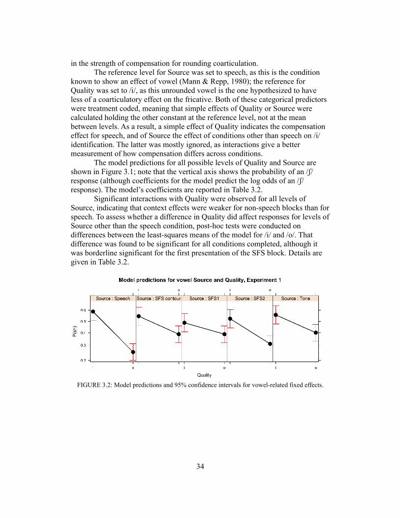
in the strength of compensation for rounding coarticulation.The reference level for Source was set to speech, as this is the condition

known to show an effect of vowel (Mann & Repp, 1980); the reference for Quality was set to /i/, as this unrounded vowel is the one hypothesized to have less of a coarticulatory effect on the fricative. Both of these categorical predictors were treatment coded, meaning that simple effects of Quality or Source were calculated holding the other constant at the reference level, not at the mean between levels. As a result, a simple effect of Quality indicates the compensation effect for speech, and of Source the effect of conditions other than speech on /i/ identification. The latter was mostly ignored, as interactions give a better measurement of how compensation differs across conditions.

The model predictions for all possible levels of Quality and Source are shown in Figure 3.1; note that the vertical axis shows the probability of an /$/ response (although coefficients for the model predict the log odds of an /$/ response). The model’s coefficients are reported in Table 3.2.

Significant interactions with Quality were observed for all levels of Source, indicating that context effects were weaker for non-speech blocks than for speech. To assess whether a difference in Quality did affect responses for levels of Source other than the speech condition, post-hoc tests were conducted on differences between the least-squares means of the model for /i/ and /o/. That difference was found to be significant for all conditions completed, although it was borderline significant for the first presentation of the SFS block. Details are given in Table 3.2.

FIGURE 3.2: Model predictions and 95% confidence intervals for vowel-related fixed effects.

34

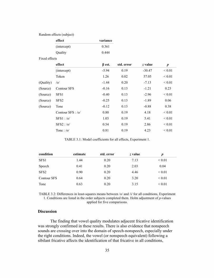
Random effects (subject)

effect variance

(intercept) 0.361

Quality 0.444

Fixed effects

effect ! est. std. error z value p

(intercept) -5.94 0.19 -30.47 < 0.01

Token 1.26 0.02 57.05 < 0.01

(Quality) /o/ -1.44 0.20 -7.13 < 0.01

(Source) Contour SFS -0.16 0.13 -1.21 0.23

(Source) SFS1 -0.40 0.13 -2.96 < 0.01

(Source) SFS2 -0.25 0.13 -1.89 0.06

(Source) Tone -0.12 0.13 -0.88 0.38

Contour SFS : /o/ 0.80 0.19 4.18 < 0.01

SFS1 : /o/ 1.03 0.19 5.41 < 0.01

SFS2 : /o/ 0.54 0.19 2.86 < 0.01

Tone : /o/ 0.81 0.19 4.23 < 0.01

TABLE 3.1: Model coefficients for all effects, Experiment 1.

condition estimate std. error z value p

SFS1 1.44 0.20 7.13 < 0.01

Speech 0.41 0.20 2.03 0.04

SFS2 0.90 0.20 4.46 < 0.01

Contour SFS 0.64 0.20 3.20 < 0.01

Tone 0.63 0.20 3.15 < 0.01

TABLE 3.2: Differences in least-squares means between /o/ and /i/ for all conditions, Experiment 1. Conditions are listed in the order subjects completed them. Holm adjustment of p-values

applied for five comparisons.

Discussion

The finding that vowel quality modulates adjacent fricative identification was strongly confirmed in these results. There is also evidence that nonspeech sounds are crossing over into the domain of speech-nonspeech, especially under the right conditions. Indeed, the vowel (or nonspeech equivalent) following a sibilant fricative affects the identification of that fricative in all conditions,

35

although the effect of the single-formant version of /o/ appears to be more reliable after listeners also completed a speech condition, and it may rely partially on listeners’ ability to associate the sound with speech. (Recall also that between the SFS condition and the first speech block, listeners were asked to associate the SFS syllables with English words.) The role of the intervening speech block may be to further activate a speech mode of perception that persists for the nonspeech stimuli. That is, listeners will perform compensation for coarticulation, an automatic process in speech perception, upon stimuli that are clearly not speech if they are primed to think of them as related to or derived from speech. One question that remains is the impact of the short SFS-to-speech matching task that listeners performed: did the forced associations with words lead to an apparent increase in vowel effect, or was it simply the completion of the task a second time (and following a speech condition)?

The positive effect of vowel in the tone block is especially interesting. The SFS stimuli share a source function with speech, differing only in the number of resonances applied, while the tone stimuli are categorically different in construction. Nevertheless, it appears that tones do trigger speech-nonspeech processing. Whether they do this by their resemblance to speech or by their resemblance to SFS is still unclear: following two conditions with SFS stimuli, could listeners have associated the tones with the formant ‘chirps’ from SFS? A better control for tones would gauge listeners’ responses before and after hearing speech and SFS conditions.

With these new questions in mind, a second experiment was designed. I outline the method and results of Experiment 2 below before returning to a discussion of the theoretical implications. As the task in Experiment 2 hews closely to that of Experiment 1, I focus primarily on the differences between the two.

Experiment 2: Method

Participants

Participants for Experiment 2 were divided into two groups. Each contained 16 participants aged 17–22 who spoke English as a native language and did not report any history of hearing or language disorders. Each group was tested on a different protocol, both of which are discussed below.

Stimuli

Stimuli similar to those from Experiment 1 were used, with a few modifications. All ‘vowels’ were the same as before, but fricatives were resynthesized. The nine-step continuum was recalculated from different endpoints—steps 2 and 8 from the old continuum—which allowed for a slightly higher

36

resolution in locating the categorical boundary.Additionally, the interpolated continuum stimuli were calculated using the

Bark scale, which should correspond more accurately to cochlear frequency resolution. Formant values for the fricatives were converted to Bark before scaling, then converted back into Hertz. Amplitude was still interpolated linearly. See the appendix for further details on these stimuli’s acoustic parameters.

Task

Experiment 2 involved two different protocols, with no subjects performing both. Subjects in Group 2 performed a task similar to the task in Experiment 1, while Group 1 performed a shorter and slightly different task. The Contour SFS condition was removed entirely for this experiment, as it did not seem to differ interestingly from the plain SFS condition.

Block 1 Block 2 Block 3 Block 4Group 1: SFS Speech SFS ToneGroup 2: Tone Speech Tone

All subjects saw a message between the second and third blocks informing them that the stimuli they were about to hear were derived from the speech sounds they just heard, although this time they were not asked to match the SFS stimuli with English words. The Tone condition was given the same treatment as the SFS condition—that is, testing before and after a speech block—to determine if association with speech would affect the results for the former in the way we saw it affecting the latter.

As in Experiment 1, stimulus presentation was random, and 7 instances of each of the 18 distinct stimuli were presented for 126 trials per block. Each block took approximately 5 minutes. A slight modification was also made to the procedure of the experiment: in addition to the labeled screen they saw in Experiment 1, subjects were given a modest visual feedback in the form of a blank screen (for 200 ms) after responding to a stimulus.

Results

As in Experiment 1, tokens at the ends of the continuum were strongly identified as one fricative or the other, suggesting a categorical response. Steps 1–3 and 7–9 were largely unambiguous, while the boundary tended to fall near steps 4–6. Recall that step 4 was less ambiguous in Experiment 1, owing to the frequency range being narrower in Experiment 2. Figure 3.3 shows the overlay of all conditions for both groups.

37

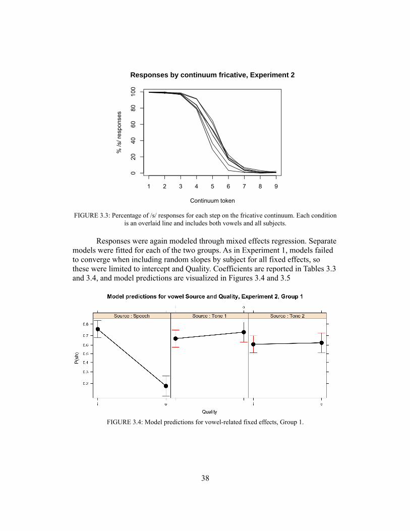
1 2 3 4 5 6 7 8 9

020

4060

80100

Responses by continuum fricative, Experiment 2

Continuum token

% /s

/ res

pons

es

FIGURE 3.3: Percentage of /s/ responses for each step on the fricative continuum. Each condition is an overlaid line and includes both vowels and all subjects.

Responses were again modeled through mixed effects regression. Separate models were fitted for each of the two groups. As in Experiment 1, models failed to converge when including random slopes by subject for all fixed effects, so these were limited to intercept and Quality. Coefficients are reported in Tables 3.3 and 3.4, and model predictions are visualized in Figures 3.4 and 3.5

FIGURE 3.4: Model predictions for vowel-related fixed effects, Group 1.

38

FIGURE 3.5: Model predictions for vowel-related fixed effects, Group 2.

Random effects (subject)

effect variance

(intercept) 0.369

Quality 0.529

Fixed effects

effect ! est. std. error z value p

(intercept) -8.76 0.33 -26.25 < 0.01

Token 1.98 0.06 32.97 < 0.01

(Quality) /o/ -2.66 0.27 -9.70 < 0.01

(Source) Tone1 -0.44 0.19 -2.35 0.02

(Source) Tone2 -0.71 0.19 -3.74 < 0.01

Tone1 : /o/ 2.96 0.28 10.53 < 0.01

Tone2 : /o/ 2.73 0.28 9.79 < 0.01

TABLE 3.3: Model coefficients for all effects, Group 1.

39

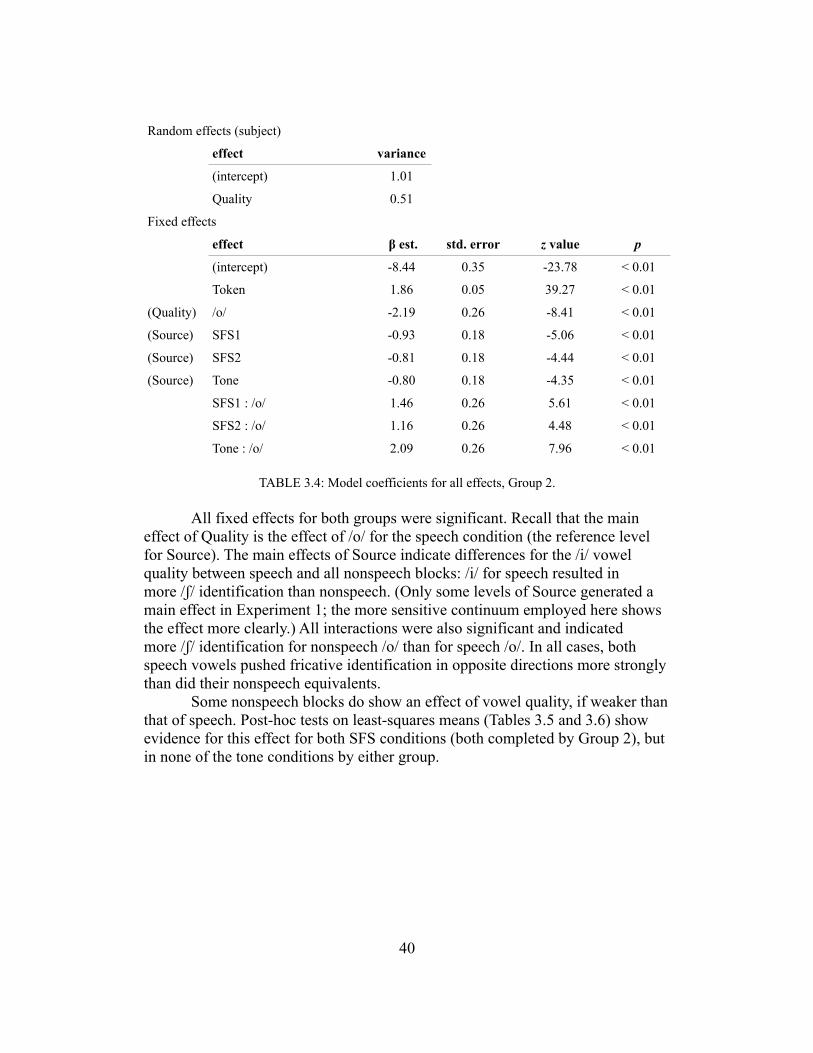
Random effects (subject)

effect variance

(intercept) 1.01

Quality 0.51

Fixed effects

effect ! est. std. error z value p

(intercept) -8.44 0.35 -23.78 < 0.01

Token 1.86 0.05 39.27 < 0.01

(Quality) /o/ -2.19 0.26 -8.41 < 0.01

(Source) SFS1 -0.93 0.18 -5.06 < 0.01

(Source) SFS2 -0.81 0.18 -4.44 < 0.01

(Source) Tone -0.80 0.18 -4.35 < 0.01

SFS1 : /o/ 1.46 0.26 5.61 < 0.01

SFS2 : /o/ 1.16 0.26 4.48 < 0.01

Tone : /o/ 2.09 0.26 7.96 < 0.01

TABLE 3.4: Model coefficients for all effects, Group 2.

All fixed effects for both groups were significant. Recall that the main effect of Quality is the effect of /o/ for the speech condition (the reference level for Source). The main effects of Source indicate differences for the /i/ vowel quality between speech and all nonspeech blocks: /i/ for speech resulted in more /$/ identification than nonspeech. (Only some levels of Source generated a main effect in Experiment 1; the more sensitive continuum employed here shows the effect more clearly.) All interactions were also significant and indicated more /$/ identification for nonspeech /o/ than for speech /o/. In all cases, both speech vowels pushed fricative identification in opposite directions more strongly than did their nonspeech equivalents.

Some nonspeech blocks do show an effect of vowel quality, if weaker than that of speech. Post-hoc tests on least-squares means (Tables 3.5 and 3.6) show evidence for this effect for both SFS conditions (both completed by Group 2), but in none of the tone conditions by either group.

40

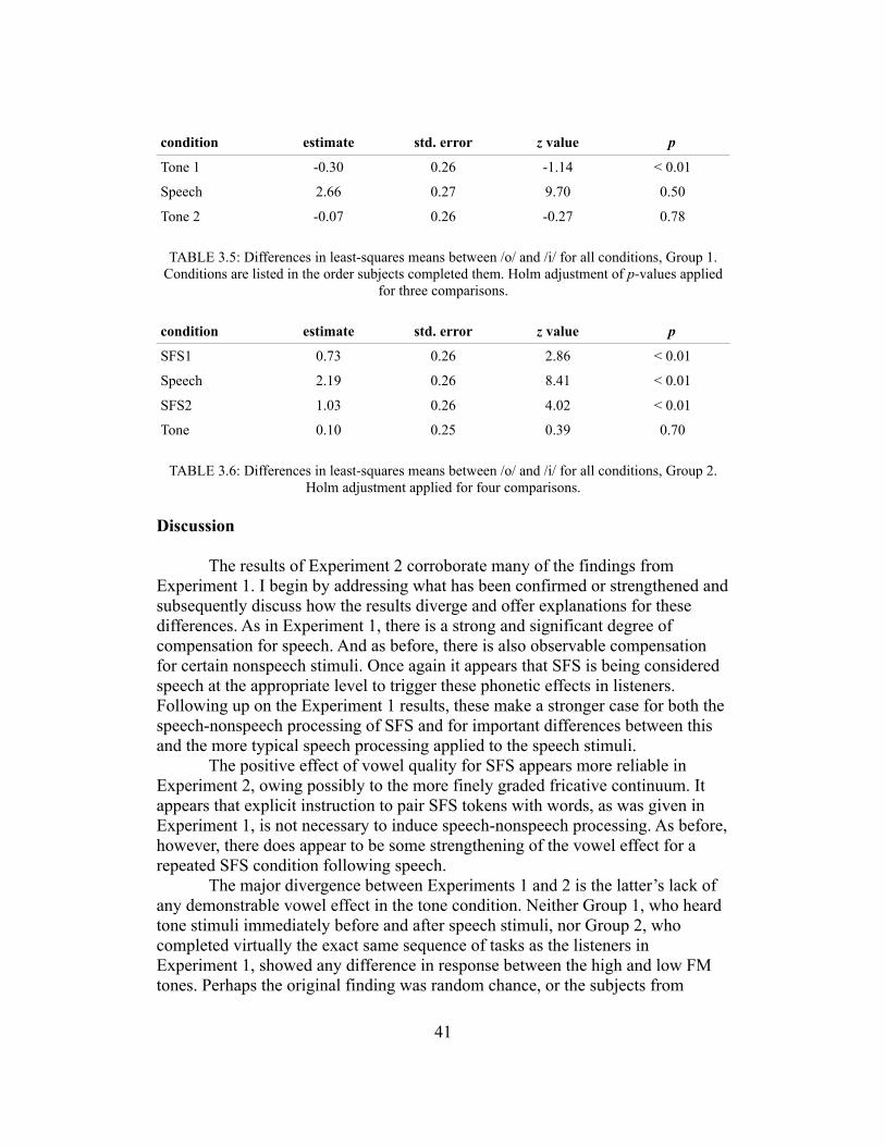
condition estimate std. error z value p

Tone 1 -0.30 0.26 -1.14 < 0.01

Speech 2.66 0.27 9.70 0.50

Tone 2 -0.07 0.26 -0.27 0.78

TABLE 3.5: Differences in least-squares means between /o/ and /i/ for all conditions, Group 1. Conditions are listed in the order subjects completed them. Holm adjustment of p-values applied

for three comparisons.

condition estimate std. error z value p

SFS1 0.73 0.26 2.86 < 0.01

Speech 2.19 0.26 8.41 < 0.01

SFS2 1.03 0.26 4.02 < 0.01

Tone 0.10 0.25 0.39 0.70

TABLE 3.6: Differences in least-squares means between /o/ and /i/ for all conditions, Group 2. Holm adjustment applied for four comparisons.

Discussion

The results of Experiment 2 corroborate many of the findings from Experiment 1. I begin by addressing what has been confirmed or strengthened and subsequently discuss how the results diverge and offer explanations for these differences. As in Experiment 1, there is a strong and significant degree of compensation for speech. And as before, there is also observable compensation for certain nonspeech stimuli. Once again it appears that SFS is being considered speech at the appropriate level to trigger these phonetic effects in listeners. Following up on the Experiment 1 results, these make a stronger case for both the speech-nonspeech processing of SFS and for important differences between this and the more typical speech processing applied to the speech stimuli.

The positive effect of vowel quality for SFS appears more reliable in Experiment 2, owing possibly to the more finely graded fricative continuum. It appears that explicit instruction to pair SFS tokens with words, as was given in Experiment 1, is not necessary to induce speech-nonspeech processing. As before, however, there does appear to be some strengthening of the vowel effect for a repeated SFS condition following speech.

The major divergence between Experiments 1 and 2 is the latter’s lack of any demonstrable vowel effect in the tone condition. Neither Group 1, who heard tone stimuli immediately before and after speech stimuli, nor Group 2, who completed virtually the exact same sequence of tasks as the listeners in Experiment 1, showed any difference in response between the high and low FM tones. Perhaps the original finding was random chance, or the subjects from

41

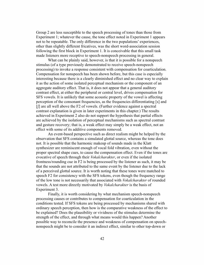
Group 2 are less susceptible to the speech processing of tones than those from Experiment 1; whatever the cause, the tone effect noted in Experiment 1 appears not to be repeatable. The only difference in the two populations’ experiences, other than slightly different fricatives, was the short word-association session following the first block in Experiment 1. It is conceivable that this small task made listeners more receptive to speech-nonspeech processing in general.

What can be plainly said, however, is that it is possible for a nonspeech stimulus (of a type previously demonstrated to receive speech-nonspeech processing) to invoke a response consistent with compensation for coarticulation. Compensation for nonspeech has been shown before, but this case is especially interesting because there is a clearly diminished effect and no clear way to explain it as the action of some isolated perceptual mechanism or the component of an aggregate auditory effect. That is, it does not appear that a general auditory contrast effect, at either the peripheral or central level, drives compensation for SFS vowels. It is unlikely that some acoustic property of the vowel is affecting perception of the consonant frequencies, as the frequencies differentiating [s] and [$] are all well above the F2 of vowels. (Further evidence against a spectral contrast explanation is given in later experiments in this chapter.) The results achieved in Experiment 2 also do not support the hypothesis that partial effects are achieved by the isolation of perceptual mechanisms such as spectral contrast and gesture recovery; that is, a weak effect may simply be a weak effect, not an effect with some of its additive components removed.

An event-based perspective such as direct realism might be helped by the observation that SFS contains a simulated glottal source, whereas the tone does not. It is possible that the harmonic makeup of sounds made in the Klatt synthesizer are reminiscent enough of vocal fold vibration, even without the proper spectral shape cues, to cause the compensation effect. Even if the tones are evocative of speech through their Vokalcharakter, or even if the isolated frontness/rounding cue in F2 is being processed by the listener as such, it may be that the sounds are not attributed to the same event by the listener due to the lack of a perceived glottal source. It is worth noting that these tones were matched to speech F2 for consistency with the SFS tokens, even though the frequency range of the low tone is not necessarily that associated with Vokalcharakter of rounded vowels. A test more directly motivated by Vokalcharakter is the basis of Experiment 3.

Finally, it is worth considering by what mechanism speech-nonspeech processing causes or contributes to compensation for coarticulation in the conditions tested. If SFS tokens are being processed by mechanisms shared with ordinary speech perception, then how is the comparative weakness of the effect to be explained? Does the plausibility or vividness of the stimulus determine the strength of the effect, and through what means would this happen? Another possible way to reconcile the presence and weakness of compensation on speech-nonspeech might be to consider it an indirect effect, similar to other top-down or

42

lexical effects that have been shown to operate in compensation for coarticulation (Elman & McClelland, 1988; Pitt & McQueen, 1998; Magnuson et al., 2003). If the speech identification of SFS context vowels occurs later to phonetic classification (or otherwise outside its path), it may be that an indirect application of this knowledge leads to a delayed and reduced effect. Theoretical consequences of this position will be considered in the general discussion.

Experiment 3

Experiments 1 and 2 demonstrated that listeners correct for rounding coarticulation on fricatives when given nonspeech with sufficient cues and/or similarity to speech. However, as noted in the previous chapter, other types of vocalic nonspeech exist—most notably, tones with clear Vokalcharakter. Could these types of tones, chosen carefully to unambiguously evoke high front vowels (high coarticulated fricative pole) and back rounded vowels (low pole), trigger the same effect?

I designed a short session to test this question directly. I hypothesized that there may be an effect of predicted vowel quality, although given the comparative weakness of the effect of SFS to that of speech, this would also be a weak effect. Although note that even if an effect of tone were to be found, it would still not be equivocal evidence of speech-nonspeech processing of the tone: a backwards contrast effect (of the type shown by Wade and Holt [2005]) may still be driving the preference for /s/ identification preceding the tone evoking /i/.

Participants

Thirteen UC Berkeley students participated in Experiment 3. None had participated in Experiments 1 or 2. None reported any history of speech or hearing disorders.

Stimuli

Stimuli were of similar type to previous experiments. There was only one session which included mixed presentation of all nine continuum steps followed either by a high tone (3 kHz) or a low tone (600 Hz). Tones were generated by a cosine function and had an amplitude envelope applied: 15 ms linear attack to full intensity (RMS of approximately four times the fricative at offset), followed by an 85 ms decay to 70% intensity and a 15 ms release. There was no gap between the fricative offset and the beginning of the tone.

Results & discussion

A mixed model was applied to the responses, with continuum token and

43

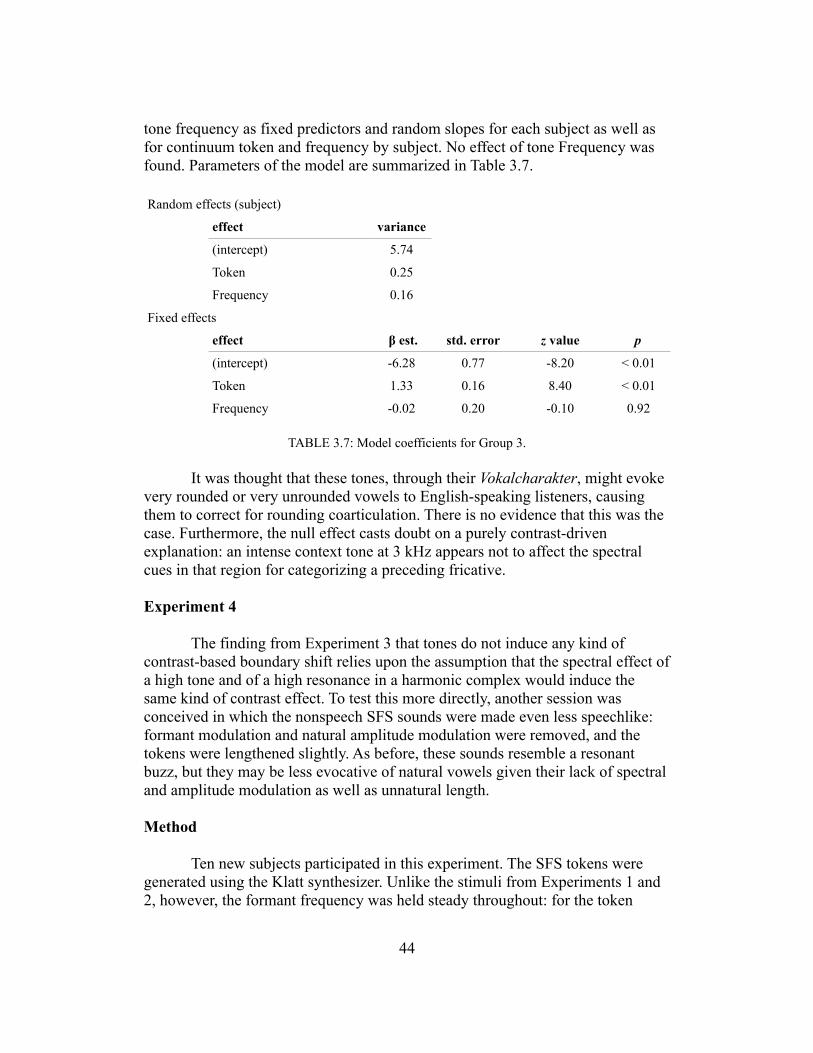
tone frequency as fixed predictors and random slopes for each subject as well as for continuum token and frequency by subject. No effect of tone Frequency was found. Parameters of the model are summarized in Table 3.7.

Random effects (subject)

effect variance

(intercept) 5.74

Token 0.25

Frequency 0.16

Fixed effects

effect ! est. std. error z value p

(intercept) -6.28 0.77 -8.20 < 0.01

Token 1.33 0.16 8.40 < 0.01

Frequency -0.02 0.20 -0.10 0.92

TABLE 3.7: Model coefficients for Group 3.

It was thought that these tones, through their Vokalcharakter, might evoke very rounded or very unrounded vowels to English-speaking listeners, causing them to correct for rounding coarticulation. There is no evidence that this was the case. Furthermore, the null effect casts doubt on a purely contrast-driven explanation: an intense context tone at 3 kHz appears not to affect the spectral cues in that region for categorizing a preceding fricative.

Experiment 4

The finding from Experiment 3 that tones do not induce any kind of contrast-based boundary shift relies upon the assumption that the spectral effect of a high tone and of a high resonance in a harmonic complex would induce the same kind of contrast effect. To test this more directly, another session was conceived in which the nonspeech SFS sounds were made even less speechlike: formant modulation and natural amplitude modulation were removed, and the tokens were lengthened slightly. As before, these sounds resemble a resonant buzz, but they may be less evocative of natural vowels given their lack of spectral and amplitude modulation as well as unnatural length.

Method

Ten new subjects participated in this experiment. The SFS tokens were generated using the Klatt synthesizer. Unlike the stimuli from Experiments 1 and 2, however, the formant frequency was held steady throughout: for the token

44

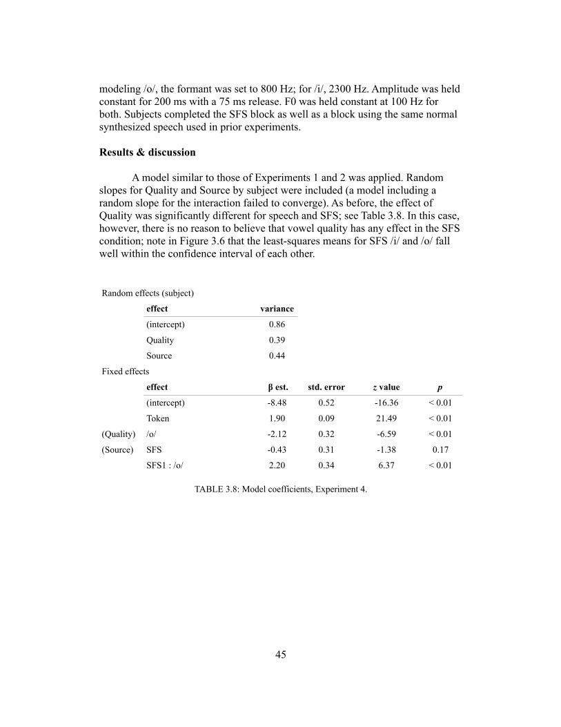
modeling /o/, the formant was set to 800 Hz; for /i/, 2300 Hz. Amplitude was held constant for 200 ms with a 75 ms release. F0 was held constant at 100 Hz for both. Subjects completed the SFS block as well as a block using the same normal synthesized speech used in prior experiments.

Results & discussion

A model similar to those of Experiments 1 and 2 was applied. Random slopes for Quality and Source by subject were included (a model including a random slope for the interaction failed to converge). As before, the effect of Quality was significantly different for speech and SFS; see Table 3.8. In this case, however, there is no reason to believe that vowel quality has any effect in the SFS condition; note in Figure 3.6 that the least-squares means for SFS /i/ and /o/ fall well within the confidence interval of each other.

Random effects (subject)

effect variance

(intercept) 0.86

Quality 0.39

Source 0.44

Fixed effects

effect ! est. std. error z value p

(intercept) -8.48 0.52 -16.36 < 0.01

Token 1.90 0.09 21.49 < 0.01

(Quality) /o/ -2.12 0.32 -6.59 < 0.01

(Source) SFS -0.43 0.31 -1.38 0.17

SFS1 : /o/ 2.20 0.34 6.37 < 0.01

TABLE 3.8: Model coefficients, Experiment 4.

45

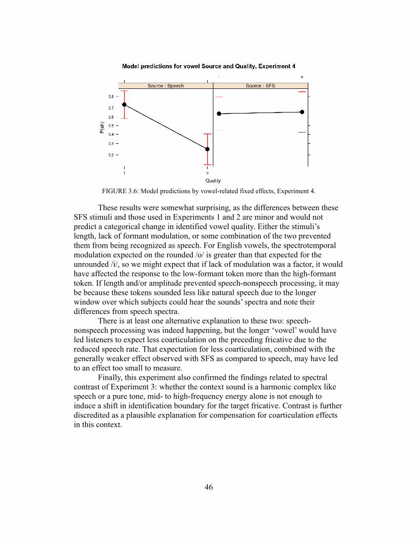
FIGURE 3.6: Model predictions by vowel-related fixed effects, Experiment 4.

These results were somewhat surprising, as the differences between these SFS stimuli and those used in Experiments 1 and 2 are minor and would not predict a categorical change in identified vowel quality. Either the stimuli’s length, lack of formant modulation, or some combination of the two prevented them from being recognized as speech. For English vowels, the spectrotemporal modulation expected on the rounded /o/ is greater than that expected for the unrounded /i/, so we might expect that if lack of modulation was a factor, it would have affected the response to the low-formant token more than the high-formant token. If length and/or amplitude prevented speech-nonspeech processing, it may be because these tokens sounded less like natural speech due to the longer window over which subjects could hear the sounds’ spectra and note their differences from speech spectra.

There is at least one alternative explanation to these two: speech-nonspeech processing was indeed happening, but the longer ‘vowel’ would have led listeners to expect less coarticulation on the preceding fricative due to the reduced speech rate. That expectation for less coarticulation, combined with the generally weaker effect observed with SFS as compared to speech, may have led to an effect too small to measure.

Finally, this experiment also confirmed the findings related to spectral contrast of Experiment 3: whether the context sound is a harmonic complex like speech or a pure tone, mid- to high-frequency energy alone is not enough to induce a shift in identification boundary for the target fricative. Contrast is further discredited as a plausible explanation for compensation for coarticulation effects in this context.

46

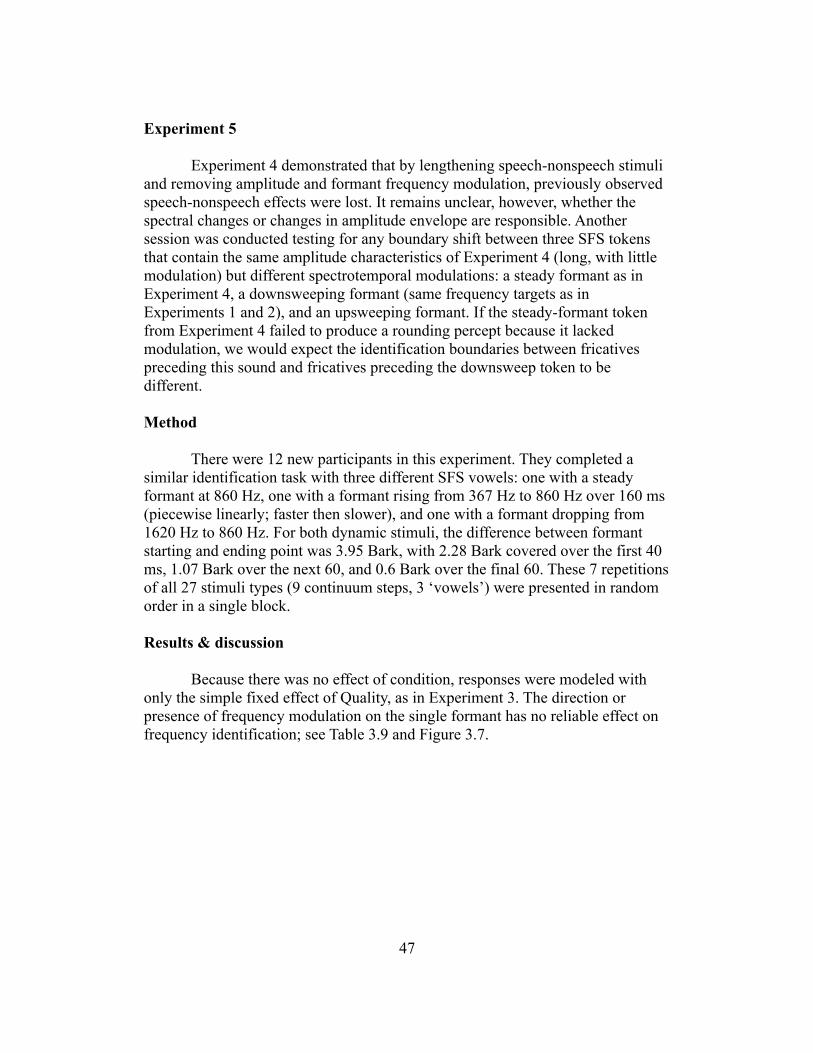
Experiment 5

Experiment 4 demonstrated that by lengthening speech-nonspeech stimuli and removing amplitude and formant frequency modulation, previously observed speech-nonspeech effects were lost. It remains unclear, however, whether the spectral changes or changes in amplitude envelope are responsible. Another session was conducted testing for any boundary shift between three SFS tokens that contain the same amplitude characteristics of Experiment 4 (long, with little modulation) but different spectrotemporal modulations: a steady formant as in Experiment 4, a downsweeping formant (same frequency targets as in Experiments 1 and 2), and an upsweeping formant. If the steady-formant token from Experiment 4 failed to produce a rounding percept because it lacked modulation, we would expect the identification boundaries between fricatives preceding this sound and fricatives preceding the downsweep token to be different.

Method

There were 12 new participants in this experiment. They completed a similar identification task with three different SFS vowels: one with a steady formant at 860 Hz, one with a formant rising from 367 Hz to 860 Hz over 160 ms (piecewise linearly; faster then slower), and one with a formant dropping from 1620 Hz to 860 Hz. For both dynamic stimuli, the difference between formant starting and ending point was 3.95 Bark, with 2.28 Bark covered over the first 40 ms, 1.07 Bark over the next 60, and 0.6 Bark over the final 60. These 7 repetitions of all 27 stimuli types (9 continuum steps, 3 ‘vowels’) were presented in random order in a single block.

Results & discussion

Because there was no effect of condition, responses were modeled with only the simple fixed effect of Quality, as in Experiment 3. The direction or presence of frequency modulation on the single formant has no reliable effect on frequency identification; see Table 3.9 and Figure 3.7.

47

FIGURE 3.7: Boundaries of SFS block in Experiment 5.

Random effects (subject)

effect variance

(intercept) 1.53

Modulation: Down 0.51

Modulation: Up 0.11

Fixed effects

effect ! est. std. error z value p

(intercept) -7.49 0.51 -14.81 < 0.01

Token 1.50 0.07 22.59 < 0.01

Modulation: Down -0.02 0.28 -0.06 0.95

Modulation: Up 0.16 0.21 0.76 0.45

TABLE 3.9: Model coefficients, Experiment 5.

Reintroducing formant frequency movement approximating natural speech does not restore speech-nonspeech processing for SFS vowels—at least not on the level needed to induce compensation for rounding coarticulation. There is no evidence that any of the three types of stimuli tested here cause listeners to consider a preceding fricative as rounded. This fact suggests that the length and steady amplitude of these SFS syllables first introduced in Experiment 4 are in fact responsible for the loss of a measurable speech-nonspeech effect. That prediction is tested in the next and final experiment.

48

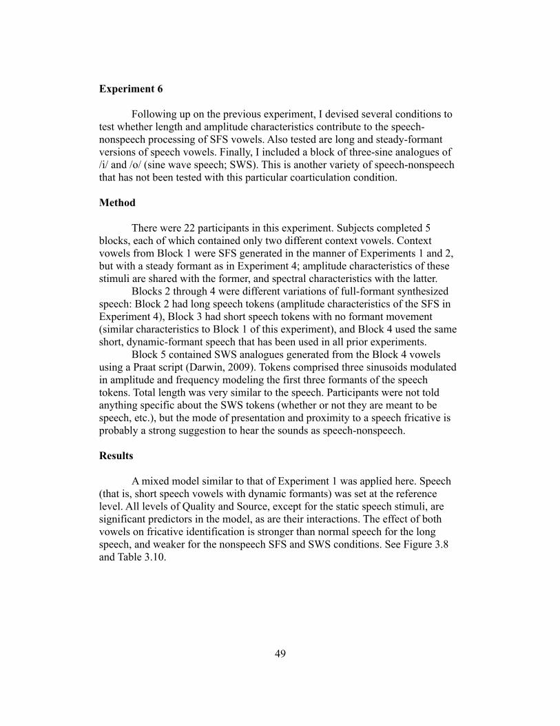
Experiment 6

Following up on the previous experiment, I devised several conditions to test whether length and amplitude characteristics contribute to the speech-nonspeech processing of SFS vowels. Also tested are long and steady-formant versions of speech vowels. Finally, I included a block of three-sine analogues of /i/ and /o/ (sine wave speech; SWS). This is another variety of speech-nonspeech that has not been tested with this particular coarticulation condition.

Method

There were 22 participants in this experiment. Subjects completed 5 blocks, each of which contained only two different context vowels. Context vowels from Block 1 were SFS generated in the manner of Experiments 1 and 2, but with a steady formant as in Experiment 4; amplitude characteristics of these stimuli are shared with the former, and spectral characteristics with the latter.

Blocks 2 through 4 were different variations of full-formant synthesized speech: Block 2 had long speech tokens (amplitude characteristics of the SFS in Experiment 4), Block 3 had short speech tokens with no formant movement (similar characteristics to Block 1 of this experiment), and Block 4 used the same short, dynamic-formant speech that has been used in all prior experiments.

Block 5 contained SWS analogues generated from the Block 4 vowels using a Praat script (Darwin, 2009). Tokens comprised three sinusoids modulated in amplitude and frequency modeling the first three formants of the speech tokens. Total length was very similar to the speech. Participants were not told anything specific about the SWS tokens (whether or not they are meant to be speech, etc.), but the mode of presentation and proximity to a speech fricative is probably a strong suggestion to hear the sounds as speech-nonspeech.

Results

A mixed model similar to that of Experiment 1 was applied here. Speech (that is, short speech vowels with dynamic formants) was set at the reference level. All levels of Quality and Source, except for the static speech stimuli, are significant predictors in the model, as are their interactions. The effect of both vowels on fricative identification is stronger than normal speech for the long speech, and weaker for the nonspeech SFS and SWS conditions. See Figure 3.8 and Table 3.10.

49

FIGURE 3.8: Model predictions for vowel-related fixed effects, Experiment 6.

Random effects (subject)

effect variance

(intercept) 0.46

Quality 1.07

Fixed effects

effect ! est. std. error z value p

(intercept) -7.56 0.23 -33.22 < 0.01

Token 1.70 0.03 53.52 < 0.01

(Quality) /o/ -1.80 0.27 -6.70 < 0.01

(Source) SFS (static) -1.21 0.15 -8.08 < 0.01

(Source) Speech (long) 0.90 0.15 5.98 < 0.01

(Source) Speech (static) -0.09 0.15 -0.60 0.55

(Source) SWS -1.14 0.15 -7.58 < 0.01

SFS (static) : /o/ 0.89 0.21 4.24 < 0.01

Speech (long) : /o/ -0.66 0.21 -3.15 < 0.01

Speech (static) : /o/ -0.25 0.21 -1.21 0.23

SWS : /o/ 1.23 0.21 5.80 < 0.01

TABLE 3.10: Model coefficients for all effects, Experiment 6.

As before, the effect of vowel for each individual condition was tested with post-hoc tests. In every condition, including all nonspeech conditions, vowel had a significant effect on fricative identification; see Table 3.11.

50

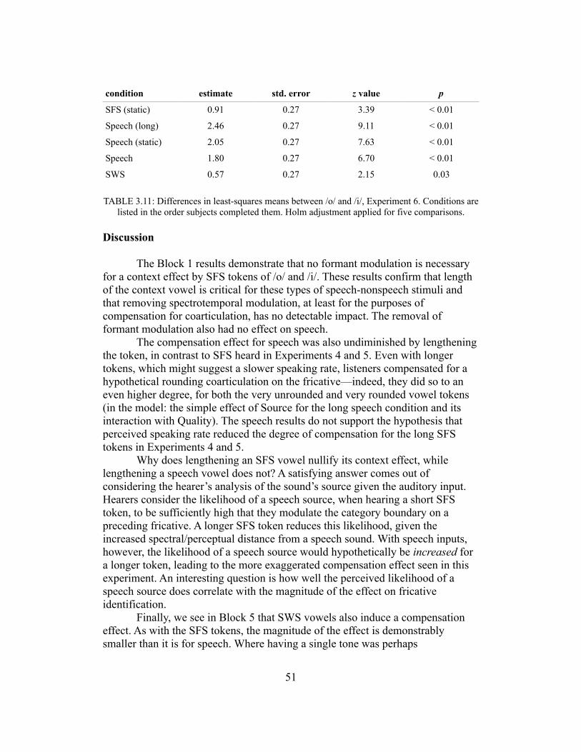
condition estimate std. error z value p

SFS (static) 0.91 0.27 3.39 < 0.01

Speech (long) 2.46 0.27 9.11 < 0.01

Speech (static) 2.05 0.27 7.63 < 0.01

Speech 1.80 0.27 6.70 < 0.01

SWS 0.57 0.27 2.15 0.03

TABLE 3.11: Differences in least-squares means between /o/ and /i/, Experiment 6. Conditions are listed in the order subjects completed them. Holm adjustment applied for five comparisons.

Discussion

The Block 1 results demonstrate that no formant modulation is necessary for a context effect by SFS tokens of /o/ and /i/. These results confirm that length of the context vowel is critical for these types of speech-nonspeech stimuli and that removing spectrotemporal modulation, at least for the purposes of compensation for coarticulation, has no detectable impact. The removal of formant modulation also had no effect on speech.

The compensation effect for speech was also undiminished by lengthening the token, in contrast to SFS heard in Experiments 4 and 5. Even with longer tokens, which might suggest a slower speaking rate, listeners compensated for a hypothetical rounding coarticulation on the fricative—indeed, they did so to an even higher degree, for both the very unrounded and very rounded vowel tokens (in the model: the simple effect of Source for the long speech condition and its interaction with Quality). The speech results do not support the hypothesis that perceived speaking rate reduced the degree of compensation for the long SFS tokens in Experiments 4 and 5.

Why does lengthening an SFS vowel nullify its context effect, while lengthening a speech vowel does not? A satisfying answer comes out of considering the hearer’s analysis of the sound’s source given the auditory input. Hearers consider the likelihood of a speech source, when hearing a short SFS token, to be sufficiently high that they modulate the category boundary on a preceding fricative. A longer SFS token reduces this likelihood, given the increased spectral/perceptual distance from a speech sound. With speech inputs, however, the likelihood of a speech source would hypothetically be increased for a longer token, leading to the more exaggerated compensation effect seen in this experiment. An interesting question is how well the perceived likelihood of a speech source does correlate with the magnitude of the effect on fricative identification.

Finally, we see in Block 5 that SWS vowels also induce a compensation effect. As with the SFS tokens, the magnitude of the effect is demonstrably smaller than it is for speech. Where having a single tone was perhaps

51

insufficiently suggestive of vowel quality to promote compensation for coarticulation (Experiments 1–3), apparently the three tones constitute enough of a spectrum for listeners to identify enough about vowel category or articulation to expect rounding, even though the acoustic source is not glottal-like as it is with SFS.

General discussion

All of the above experiments constitute ample evidence for speech-nonspeech playing a role in compensation for coarticulation, a relatively low-level phenomenon in perception. This case is made through evidence of compensation with nonspeech stimuli and lack of evidence for compensation given acoustically similar nonspeech stimuli. At least two types of sounds, SFS and SWS, are able to trigger compensation. They do so, however, to a markedly smaller degree than more natural-sounding speech. Additionally, slight lengthening of the SFS stimuli was found to remove the effect entirely, even though these same modifications bolstered the effect when applied to speech stimuli.

Beyond the first experiment, pure tones never caused a significant shift in identification boundary on the preceding fricative, whether set to frequencies that have been shown to evoke /i/ and /u/~/o/ or matched to the F2 of the speech or SFS stimuli. Despite their spectral simplicity, pure tones have been shown to show speech-nonspeech processing through their Vokalcharakter (as discussed in Chapters 2 and 4). It is conceivable, then, that they may have been processed as speech and entered into compensation for coarticulation. That they are not may have to do with their weak spectral cues: SWS with three tonal analogues of speech formants, and thus a much richer spectral representation, does have a positive effect. A richer spectral representation is also present in SFS, despite having the same pole cue as a pure tone, which suggests that a more broadband spectrum helps to provide a solid phonetic identification. The synthetic glottal source of SFS may also have provided a solid basis for phonetic processing, or may have made it easier for listeners to attribute the fricative and speech to a single talker.

Weak effects and absent effects

Despite the reliability for SFS to shift the fricative boundary, the effects of SFS and SWS are consistently determined to be smaller than that induced by speech. Typically, nonspeech stimuli in this type of condition elicit a ‘partial’ effect, or one of lesser magnitude than might be expected with speech. The size of the effect may be informative, and may reflect different mechanisms for compensation applying additively, such as masking, central contrast mechanisms, and recovery of articulatory gestures (Johnson, 2011; Mitterer, 2006; Holt &

52

Lotto, 2002). However, the experiments here found no other evidence that different motivating conditions for compensation were ever isolated: certain nonspeech sounds that should have had sufficient spectral energy to induce purely auditory effects had no measurable effect whatsoever. If these weaker effects are actually partial versions of some full-speech effects, the constituent causes are unclear and seem not to be separable along the lines of phonetic versus purely auditory compensation.

An alternative explanation for the weakness of the effects rests on their status as nonspeech. Note from the review in Chapter 2 that phonetic judgments on nonspeech sounds are generally always less uniform across listeners than for speech sounds. Even when clearly evocative of speech categories, nonspeech sounds lack all the cues necessary for a confident match. It may be that the inexactness of the match also prompts a conservative compensatory response: without clear knowledge of the segment being heard, and thus without clear knowledge of the gestures needed to create it, the perceptual system ‘hedges’ and produces a weak effect. With vivid, clearly identifiable speech, no tempering of the effect is necessary. Under this view, the magnitude of the effect could be independently modulated by the actual phonetics and by the quality of the signal.

These weakened effects allow some room for speculation. But probably the most puzzling finding of these experiments is the lack of effect for long SFS vowels. In every case except one in Experiment 1, where the fricative continuum was less sensitive, short SFS tokens produced a reliable shift; the longer tokens, there is no evidence for a shift of any size. The only explanation I can offer is that a long SFS token is so obviously nonspeech that it fails to stream with the fricative and the two are not perceived as a single phonetic event. The length of the window during which the auditory system has time to consider the unnaturalness of the sound and its suspicious lack of certain spectral cues could be the difference in accepting the sound as speech and rejecting it.

Recall also that providing speechlike, acoustically plausible spectrotemporal transitions into the vowels appears not to be important either for speech or for SFS stimuli. Although a formant in motion lends the sound an unmistakable quality of speech, even for short stimuli, this enhancement does not carry over into the compensation effect. It seems that listeners are entirely capable of filling in plausible transitions and matching sounds to native-language vowel categories, so long as the length and amplitude of the sound allow it.

Theories of speech perception

As with all speech-nonspeech phenomena, the findings of this chapter pose a difficulty for direct realism and other approaches that rely on the direct perception of articulation events: with a decidedly nonspeech sound and no detectable lossy channel or environment—indeed, the adjacent fricative is pristine—listeners cannot be said to be directly perceiving a natural occurrence or any

53

cues that would cause them to reconstruct one. Nevertheless, the sounds do have demonstrable phonetic value. Details of the vowels’ articulations are crucial to predicting their acoustic effects on the preceding fricative, suggesting that listeners do indeed understand the gestures underlying these sounds; still, they cannot be perceiving them directly, but must rather match a sound to an articulation, evidently by its acoustic similarity.

Auditory approaches to speech perception are somewhat compatible with these results but also face some difficulties. The null effect of pure tones and of longer SFS tokens seriously discounts an account of compensation, for this paradigm, that relies on auditory phenomena such as spectral contrast. These results leave little doubt that some extra-auditory phonetic percept is needed to perform compensation. The basis of that phonetic percept appears to follow directly from certain key acoustic features, which do not depend on an identifiable speech source to be processed as speech.

As far as the actual mechanisms that are in play that enable nonspeech to have unambiguously phonetic effects on speech, there are at least two possibilities. Either nonspeech is being processed as speech using ordinary speech perception mechanisms, or some higher-level phonetic or phonemic representation is being accessed at some point following normal phonetic identification and acting upon identification of the fricative in top-down fashion. If the latter is the case, it implies that speech perception is for some reason taking either a second pass at the stimuli, or a late pass following initial processing that does not consider it speech. This choice would require an explanation either for why the perceptual system is making two passes over the same event or for why, in the context of a quickly predictable experimental setting, subjects did not begin to process the stimuli as speech after only a few trials. These complications are not entirely damning for this possibility, although they suggest that the first possibility, that speech perception admits and acts upon nonspeech sounds, is correct.

Revisiting the use of SFS in compensation for perseverative coarticulation

The experiments discussed above are not the first foray into using SFS as drivers of compensation for coarticulation: using the /da/~/ga/ paradigm from Mann (1980), Lotto and colleagues (2003) tested listeners using SFS precursor syllables. The formant trajectory for the nonspeech context syllables was based on F3 of [l] and [%]. They found an effect in the same direction as would be predicted by the full speech sounds and by tones modeling F3.

Recall that in this chapter’s Experiment 1, subjects were asked to identify the SFS tokens as one of five vowels (English /i/, /e/, /a/, /u/, /o/) and overwhelmingly identified the high-formant token as a front vowel and the low-formant token as a back vowel.1 Could the Lotto et al. results, then, be driven by

1 I would also like to note that although Lotto et al. claim that these sounds ‘certainly contain no

54

speech-nonspeech perception of the precursors as front and back vowels? Coarticulation with front vowels would lead to the fronting of /g/, which could reduce the acoustic dissimilarity of [di] and [gi] and drive compensation.

I conducted an additional pilot experiment to confirm that [i] and [u] precursors shift the identification boundary between /d/ and /g/. Using a procedure similar to the experiments in this chapter, I tested two precursor vowels on an 8-step /da/~/ga/ continuum, with seven repetitions of each of the 16 possible tokens. The precursor tokens were full-formant vowels with F2 identical to the single formants from Lotto et al.’s stimuli in their Experiment 1; I would transcribe these sounds phonetically as [ij] and [iu]. With 11 subjects, a large and reliable separation of an interpolated hypothetical category boundary between the two was found (1.5 step mean difference; t = 4.69, p < 0.01). It is likely, then, that the boundary separation observed in this part of the Lotto et al. study is actually driven by speech-nonspeech processing on the SFS context syllables rather than by purely auditory effects.

Conclusion

The findings described in this chapter fit with the greater body of work demonstrating how nonspeech sounds can be heard as speech, and what this fact can tell us about ordinary speech perception. The major contribution is to show that speech-nonspeech processing enters into pre-attentive phonetic identification. Thus, speech-nonspeech appears to be driven by ordinary mechanisms of speech production. The task remains to adequately model and predict the weakness of the effect for nonspeech. This result is compatible with an approach in which phonetic labels are ‘weighted’ according to some confidence criterion based on the plausibility or robustness of a match with the acoustic input, and this weight is carried into further phonetic processing. Adapting this intuition into a model for spectral recognition is the major focus of Part III of this dissertation.

Before that discussion, however, Chapter 4 will present further speech-nonspeech data, employing a more sensitive method to address tonal stimuli, which failed to generate observable effects in this chapter. Further evidence will be given for the tight integration of speech perception and speech-nonspeech. Continuing the theme established here, spectrum will be key for tonal speech-nonspeech, and the handling of temporally complex stimuli can be predicted to some degree by a simple consideration of spectral targets. The experiments in this chapter and the next, following up on the review in Chapter 2, set up the spectral similarity criteria that are elaborated and defined further in the final two chapters.

identifiable phonemic content’ (2003:54), the survey from my own experiment found clear tendencies for the phonemes most readily associated with these types of sounds. An assertion that these sounds cannot have phonemic value may be based on the assumption that nonspeech sounds cannot in general—which, given the evidence for speech-nonspeech processing given in Chapter 2 and throughout this dissertation, is not a safe assumption.

55

Chapter 4Tone-evoked vowels and semivowels

As seen in Chapter 2, the intelligibility of words and sentences is certainly a sufficient criterion for nonspeech being recognized as speech, but the parity between speech and nonspeech sounds can be much more subtle. Probably the most extreme case of a speech percept drawn from a decidedly nonspeech acoustic stimulus is the phenomenon by which single pure tones of different frequencies resemble different vowels to a listener, with lower tones generally being identified with back vowels and higher tones (in the range of 1.5 to 4 kHz) with front vowels. The correspondence between vowels and tones is not as robust as that between speech and more spectrally complex nonspeech, but past studies have shown the association to be predictable and repeatable. This phenomenon, which I call Vokalcharakter following Köhler (1910), has received sporadic attention for some time but is lacking both a comprehensive review and an adequate explanation; this paper seeks to remedy the first point and offer direction towards addressing the second. I will also present results of original experiments and discuss their relevance to what is currently known. I begin, however, with the review of Vokalcharakter, followed by a discussion of experiments with acoustically similar stimuli—most notably, filtered vowels and sine wave speech (SWS).

Tones and vowels

Although the earliest systematic studies appear in the early 20th century, the relationship between vowel quality and a single frequency peak was remarked upon much earlier. Referring to photostats of Isaac Newton’s original notebooks (c. 1665), Ladefoged (1967, p. 65) transcribes: ‘The filling of a very deepe flaggon wth a constant streame of beere or water sounds ye vowells in this order w, u, !, o, a, e, i, y’ (the symbols are Ladefoged’s best printed equivalents to Newton’s handwriting). Helmholtz (1954; final German version, 1877) notes that the major resonance of the back vowels from high to low constitute an ascending series of tones, which is continued by the higher resonance of the front vowels from low to high. Köhler (1910; as summarized by Weiss, 1920) ascribed the property of Vokalcharakter to pure tones, with categories occurring roughly every octave: 256 Hz corresponds to [u], 526 Hz to [o], and 1066 Hz to [a].

Weiss (1920) carried out what is probably the earliest systematic experimental mapping between pitches and vowels, asking listeners to match the sounds of tuning forks (ranging from 128 to 1152 Hz) with one of eight vowels. Unfortunately, Weiss’s results are difficult to interpret due to high test/retest variability, as well as variability between the populations studied. (Note also that the sounds of tuning forks do not have the same spectral or temporal

56

characteristics of constant-amplitude pure tones.) The most thorough study for English is by Farnsworth (1937), who played tones ranging from 375 to 2400 Hz generated by a beat frequency oscillator and asked listeners to identify the vowel. The most common vowel choices were [u], [o], and [i], for which the respective median frequencies were 500, 550, and 1900 Hz; ["] and [!] had medians of 700 and 825 Hz and, if lumped together, constitute the fourth most common choice. Overall, the results suggest a continuum similar to Newton’s.

Systematic research on Vokalcharakter is, happily, not restricted to English. Engelhardt and Gehrcke (1930) address German vowels, Fant (1973) Swedish vowels, and Chiba and Kajiyama (1958) Japanese vowels. (Note that the latter study does not directly test the mapping between pitch and vowel but does identify a ‘principal formant’ that characterizes each of the five Japanese vowels and speculates that this alone is sufficient to identify the vowel.) The availability of these languages is actually quite fortuitous because all feature rounded front or unrounded back vowels, and a natural question to ask from the English data alone would be how rounding changes a vowel’s associated tone. Results show that the effect of rounding is dwarfed by that of place: the German and Swedish studies indicate that [y] tends to favor a slightly lower tone than [i] but not as low as [e] (Fant’s results show that central [&] is rarely associated with any tone), and the supposed unique principal formant of Japanese ['] is still hypothesized to be lower than that of [o] (350 vs. 500 Hz). The Fant and Engelhardt studies are also valuable because they include responses to tones of up to 4 kHz, and both show that listeners overwhelmingly choose [i] above 3 kHz, while [y] dominates in the 2 to 3 kHz range. How the boundaries between front vowels differ for speakers of languages without rounded front vowels—or, put another way, what English-speaking listeners would do with the space that German and Swedish listeners seem to allocate to [y]—is a question that would probably require direct study of both speaker groups with very high tones.

The studies mentioned above have relied on imagined vowels, usually by presenting listeners with a word bank, one with each possible vowel response. Kuhl et al. (1991) showed that this phenomenon can also operate across modalities: given video-only presentations of spoken vowels, listeners tended to match an [!] face with lower tones (750, 1000, or 1500 Hz) and an [i] face with higher tones (2, 3, or 4 kHz). The results from the audiovisual condition qualitatively matched those with imagined speech and also recorded vowels. Though their study tested only [i] and [!] productions, the audiovisual presentation method is extensible to the entire continuum of tone-evoked vowels for English speakers, as there are salient and generally unambiguous visual articulation for three broad categories: mid/high front vowels, with high jaw and lips unrounded or even wide; low vowels, with open jaw; and mid/high back vowels, with lips more rounded than for other vowels.

Kuhl et al. name this phenomenon ‘predominant pitch’. I deviate from their terminology for two major reasons: first, to stress that the imagined vowel is

57

triggered perceptually by the tone, and not that the vowel has an inherent pitch; ‘predominant pitch’ seems to suggest the latter, which may be confusable with the tendency for vowels high in the space to be produced with a higher rate of vocal fold vibration. Second, it is important to avoid ascribing tonal Vokalcharakter to pitch in the psychoacoustic sense, which I contend is independent of the spectral analysis at the root of the effect. That pitch and spectrum can be perceived from the same tonal stimulus has actually been demonstrated for SWS: Remez and Rubin (1993) show that the acoustic correlate of perceived intonation in SWS sentences is the first formant analogue, which also contributes to the intelligibility of the stimulus. For the remainder of this paper, the term ‘pitch’ is reserved for its psychophysical sense, and the rate of oscillation of a simple tone will always be described as its ‘frequency’.

Similar sounds

Can Vokalcharakter be explained entirely by the spectral characteristics of the tone itself? To answer this question it is helpful to consider experiments on the identification of filtered vowels. Though speech is complex and broadband, filtered speech will approach a pure tone with the narrowing of the passband. If identification of narrowband-filtered vowels matches tone-evoked vowels for that range, it would bolster the intuition that the effect is spectral in nature. (Speech intelligibility under certain filtering conditions has also been studied extensively; see Cunningham [2003] for a review. For the purposes of studying Vokalcharakter, I am concerned here specifically with identification of isolated vowels.)

An early study of filtered vowels was conducted by Lehiste and Peterson (1959), who asked listeners to identify low- and high-pass filtered English vowels at cutoff frequencies from 550 to 4800 Hz. With high-pass cutoffs at and above 2100 Hz, vowel were overwhelmingly identified as [i] or, less commonly, the tense front [e(]. When low-pass filtering the vowels at 540 Hz, nearly all tokens were identified as a back rounded vowel [u], [)], [o)], or ["]. (Results were similar for low-pass 950 Hz, although [!] was usually identified correctly in this case.) These results match those from tonal Vokalcharakter: low tones, especially under 1 kHz, strongly evoke back vowels like [u] and [o)], while high tones evoke [i], even those tones much higher than the dominant spectral peak of [i]. Shriberg (1992) finds similar confusions for vowels filtered at 1 kHz: with low-pass filtering, front vowels are often identified as back or central vowels, and with high-pass filtering, back vowels are likely to be misidentified as central or front.

Missing so far is an equivalent to mid-range tones, which would be better characterized by band-pass filtering. Chiba and Kajiyama (1958) apply several filtering strategies to Japanese vowels and make the identification judgments themselves. One of their conclusions is that ‘every vowel turns into a or ao with B. P. 900—1600’ (p. 208). Taking these studies together, it appears that the three

58

most common broad Vokalcharakter categories I noted in Farnsworth’s and Fant’s results—mid/high back vowels, low vowels, and mid/high front vowels—can all be predicted by the phonetic quality of filtered vowels, with the center of the passband roughly corresponding to tone frequency.

Frequency modulation

Prior research on Vokalcharakter has been limited to steady tones evoking spectra of single vowels. If the phenomenon is due to the same mechanism underlying speech perception, as it appears to be, then it should also be possible to observe speech percepts associated with frequency-modulated (FM) tones. This has been done extensively with multi-tone complexes in SWS, which usually features three tones continually modulating in both frequency and amplitude to match the frequency and bandwidth of formants in the speech from which it was generated. For longer utterances, particularly those with few obstruents, SWS is highly intelligible. When dropping to a single formant analogue, however, virtually all intelligibility is lost (Remez et al., 1981). When presenting the formants separately, there is evidence that F2 contributes the most to intelligibility: when presenting unaltered video of speech with single-formant sinusoidal analogues, Saldaña et al. (1996) show that more correct syllables are identified when a sine-wave analogue of F2 is present, but not when either F1, F3, or signal-correlated noise is present.

For FM tones to consistently evoke speech sounds, however, they may have to be designed more deliberately than selecting SWS components. I designed such stimuli and tested their associability to speech using the visual modality, in a paradigm with some similarities to Kuhl et al. (1991). The experiments described in the remainder of this paper extend Vokalcharakter to semivowels and investigate the interactions between vowel and semivowel identification within the same syllable.

Experiment 1

If tones with dynamic frequency can have Vokalcharakter, then the natural analogical extension is from vowels to semivowels—segments with vowel-like acoustics but with rapid change. An obvious choice for semivowel to test is [w]: its early portion is acoustically virtually identical to [u], which is strongly evoked by low tones; it is extremely visually prominent, as it involves a transition from the lips being unrounded to rounded; and it is in the phonological inventory of American English speakers, who were recruited as subjects.

To present a clear visible [w] with context, video of the CV syllable [w!] was filmed; as a similar case without the rounded semivowel, [b!] was also filmed. Vokalcharakter predicts that [w!] should match perceptually with a tone that starts low and rises. I also hypothesized that the rate of FM should impact

59

how well the tone evokes a glide versus a more rapid event, such as formant transitions from a stop closure: generally speaking, it should be expected that the total duration of detectable frequency modulation should match the duration of detectable visual modulation—i.e., lip movement. FM tones can be varied in a number of ways, which are discussed in detail below; by asking subjects to choose between the two speech videos as a match for a variety of FM tone types, it is possible to model their choice of visual syllable as a function of the controllable acoustic properties of the tone.

Method

Subjects

Volunteers were recruited from the undergraduate student population of UC Berkeley. 28 subjects were recruited and split evenly into two groups. Each group performed an identical task with minor differences in the stimuli between the two. No subjects reported any history of language or hearing disorders. Participants were compensated with either cash or extra credit for an introductory linguistics course.

Stimuli

All stimuli were short video clips (1.25 s), with the video and audio tracks generated separately. Videos were unaltered clips of a 27-year-old male native speaker of American English pronouncing CV syllables in isolation. The articulation was exaggerated very slightly for visual clarity. Videos were cropped to a 360x360 resolution and compressed using lossy (MPEG) compression. Compression artifacts were minor and did not in any way obscure the phonetics of the image. When presented as stimuli, videos were uniformly stretched to fill the vertical dimension of the computer screen.

The audio from the original video recording was discarded and replaced with synchronized FM tones. These tones were of the same approximate length as the spoken syllables and were aligned manually by the experiment designer for best impressionistic coherence with the video, with the ultimate result being a video of a person who appeared to be uttering FM tones. (Audio was originally aligned automatically with video using an amplitude threshold of the original audio track as recorded by the video camera; however, the variability in the audio track, due in part to intrinsic vowel amplitude, led to some AV combinations looking much more plausible than others due only to the timing of tone onset, which was not what this experiment was designed to measure.)

The FM tones were generated from scratch as a function of time. The instantaneous angular frequency ! of a tone was defined as a logistic function of time, with a minimum approaching the starting frequency of the tone !s and a

60

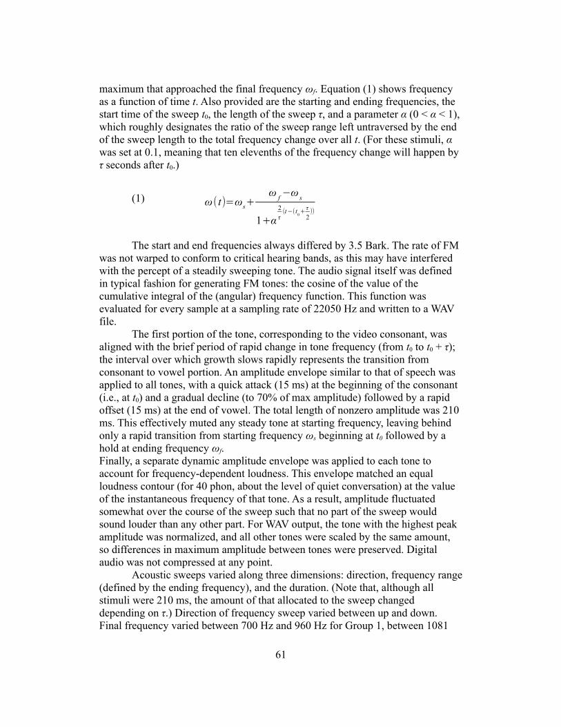
maximum that approached the final frequency !f. Equation (1) shows frequency as a function of time t. Also provided are the starting and ending frequencies, the start time of the sweep t0, the length of the sweep ", and a parameter # (0 < # < 1), which roughly designates the ratio of the sweep range left untraversed by the end of the sweep length to the total frequency change over all t. (For these stimuli, # was set at 0.1, meaning that ten elevenths of the frequency change will happen by " seconds after t0.)

(1) !( t)=!s+! f!! s

1+!2"(t!(t

0+ !

2))

The start and end frequencies always differed by 3.5 Bark. The rate of FM was not warped to conform to critical hearing bands, as this may have interfered with the percept of a steadily sweeping tone. The audio signal itself was defined in typical fashion for generating FM tones: the cosine of the value of the cumulative integral of the (angular) frequency function. This function was evaluated for every sample at a sampling rate of 22050 Hz and written to a WAV file.

The first portion of the tone, corresponding to the video consonant, was aligned with the brief period of rapid change in tone frequency (from t0 to t0 + !); the interval over which growth slows rapidly represents the transition from consonant to vowel portion. An amplitude envelope similar to that of speech was applied to all tones, with a quick attack (15 ms) at the beginning of the consonant (i.e., at t0) and a gradual decline (to 70% of max amplitude) followed by a rapid offset (15 ms) at the end of vowel. The total length of nonzero amplitude was 210 ms. This effectively muted any steady tone at starting frequency, leaving behind only a rapid transition from starting frequency "s beginning at t0 followed by a hold at ending frequency "f.Finally, a separate dynamic amplitude envelope was applied to each tone to account for frequency-dependent loudness. This envelope matched an equal loudness contour (for 40 phon, about the level of quiet conversation) at the value of the instantaneous frequency of that tone. As a result, amplitude fluctuated somewhat over the course of the sweep such that no part of the sweep would sound louder than any other part. For WAV output, the tone with the highest peak amplitude was normalized, and all other tones were scaled by the same amount, so differences in maximum amplitude between tones were preserved. Digital audio was not compressed at any point.

Acoustic sweeps varied along three dimensions: direction, frequency range (defined by the ending frequency), and the duration. (Note that, although all stimuli were 210 ms, the amount of that allocated to the sweep changed depending on !.) Direction of frequency sweep varied between up and down. Final frequency varied between 700 Hz and 960 Hz for Group 1, between 1081

61

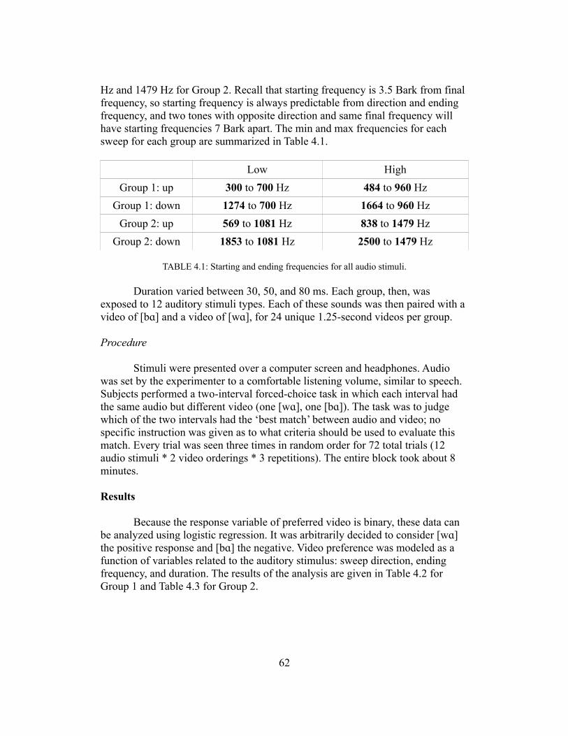
Hz and 1479 Hz for Group 2. Recall that starting frequency is 3.5 Bark from final frequency, so starting frequency is always predictable from direction and ending frequency, and two tones with opposite direction and same final frequency will have starting frequencies 7 Bark apart. The min and max frequencies for each sweep for each group are summarized in Table 4.1.

Low HighGroup 1: up 300 to 700 Hz 484 to 960 Hz

Group 1: down 1274 to 700 Hz 1664 to 960 HzGroup 2: up 569 to 1081 Hz 838 to 1479 Hz

Group 2: down 1853 to 1081 Hz 2500 to 1479 Hz

TABLE 4.1: Starting and ending frequencies for all audio stimuli.

Duration varied between 30, 50, and 80 ms. Each group, then, was exposed to 12 auditory stimuli types. Each of these sounds was then paired with a video of [b!] and a video of [w!], for 24 unique 1.25-second videos per group.

Procedure

Stimuli were presented over a computer screen and headphones. Audio was set by the experimenter to a comfortable listening volume, similar to speech. Subjects performed a two-interval forced-choice task in which each interval had the same audio but different video (one [w!], one [b!]). The task was to judge which of the two intervals had the ‘best match’ between audio and video; no specific instruction was given as to what criteria should be used to evaluate this match. Every trial was seen three times in random order for 72 total trials (12 audio stimuli * 2 video orderings * 3 repetitions). The entire block took about 8 minutes.

Results

Because the response variable of preferred video is binary, these data can be analyzed using logistic regression. It was arbitrarily decided to consider [w!] the positive response and [b!] the negative. Video preference was modeled as a function of variables related to the auditory stimulus: sweep direction, ending frequency, and duration. The results of the analysis are given in Table 4.2 for Group 1 and Table 4.3 for Group 2.

62

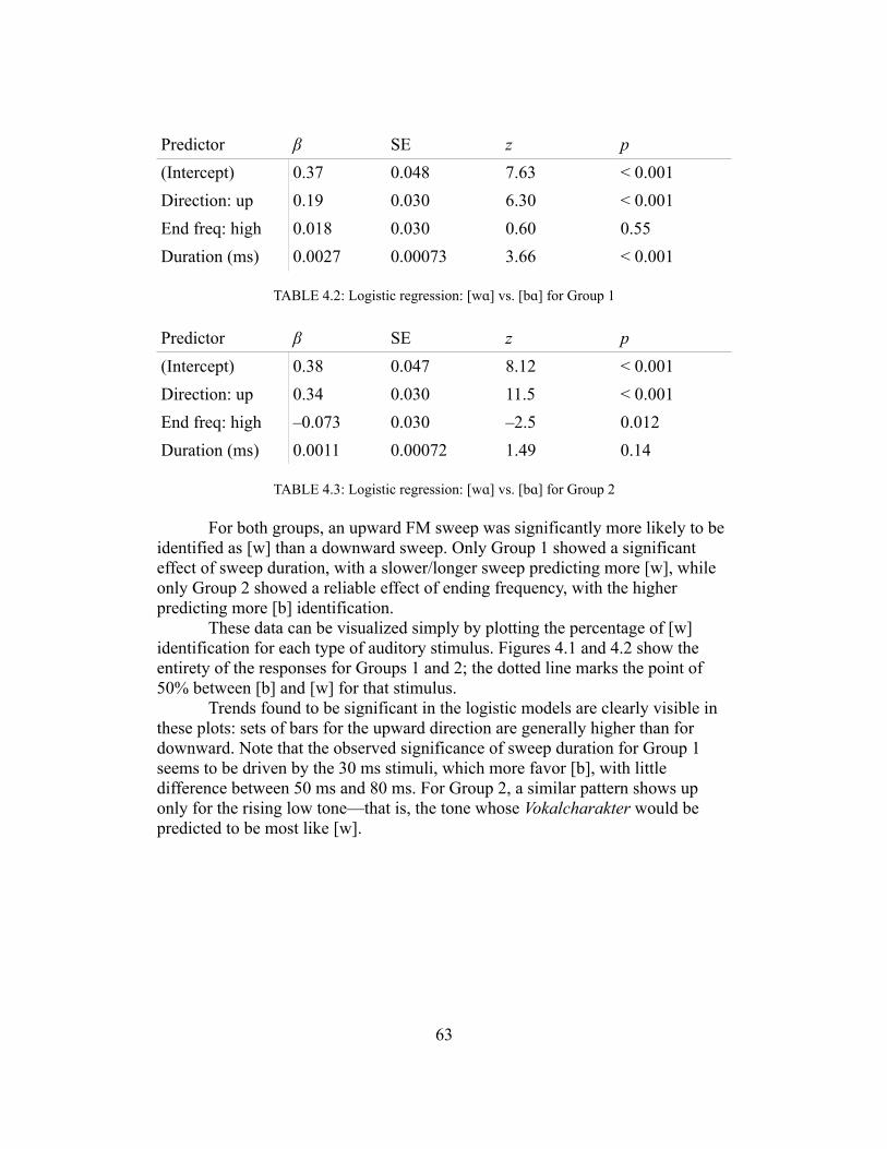
Predictor # SE z p(Intercept) 0.37 0.048 7.63 < 0.001Direction: up 0.19 0.030 6.30 < 0.001End freq: high 0.018 0.030 0.60 0.55Duration (ms) 0.0027 0.00073 3.66 < 0.001

TABLE 4.2: Logistic regression: [w!] vs. [b!] for Group 1

Predictor # SE z p(Intercept) 0.38 0.047 8.12 < 0.001Direction: up 0.34 0.030 11.5 < 0.001End freq: high –0.073 0.030 –2.5 0.012Duration (ms) 0.0011 0.00072 1.49 0.14

TABLE 4.3: Logistic regression: [w!] vs. [b!] for Group 2

For both groups, an upward FM sweep was significantly more likely to be identified as [w] than a downward sweep. Only Group 1 showed a significant effect of sweep duration, with a slower/longer sweep predicting more [w], while only Group 2 showed a reliable effect of ending frequency, with the higher predicting more [b] identification.

These data can be visualized simply by plotting the percentage of [w] identification for each type of auditory stimulus. Figures 4.1 and 4.2 show the entirety of the responses for Groups 1 and 2; the dotted line marks the point of 50% between [b] and [w] for that stimulus.

Trends found to be significant in the logistic models are clearly visible in these plots: sets of bars for the upward direction are generally higher than for downward. Note that the observed significance of sweep duration for Group 1 seems to be driven by the 30 ms stimuli, which more favor [b], with little difference between 50 ms and 80 ms. For Group 2, a similar pattern shows up only for the rising low tone—that is, the tone whose Vokalcharakter would be predicted to be most like [w].

63

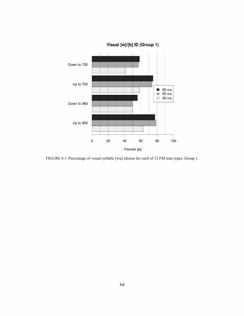
FIGURE 4.1: Percentage of visual syllable [w!] chosen for each of 12 FM tone types, Group 1.

64

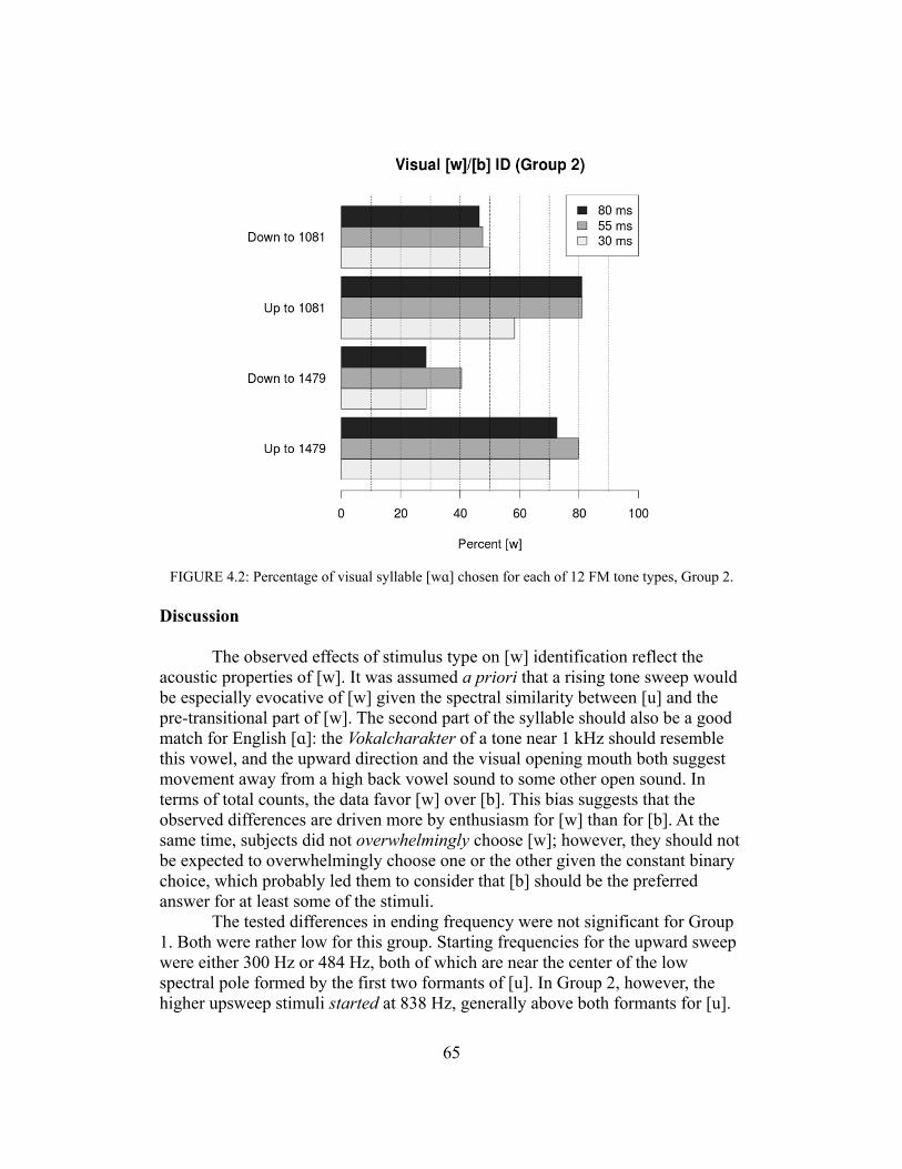
FIGURE 4.2: Percentage of visual syllable [w!] chosen for each of 12 FM tone types, Group 2.

Discussion

The observed effects of stimulus type on [w] identification reflect the acoustic properties of [w]. It was assumed a priori that a rising tone sweep would be especially evocative of [w] given the spectral similarity between [u] and the pre-transitional part of [w]. The second part of the syllable should also be a good match for English [!]: the Vokalcharakter of a tone near 1 kHz should resemble this vowel, and the upward direction and the visual opening mouth both suggest movement away from a high back vowel sound to some other open sound. In terms of total counts, the data favor [w] over [b]. This bias suggests that the observed differences are driven more by enthusiasm for [w] than for [b]. At the same time, subjects did not overwhelmingly choose [w]; however, they should not be expected to overwhelmingly choose one or the other given the constant binary choice, which probably led them to consider that [b] should be the preferred answer for at least some of the stimuli.

The tested differences in ending frequency were not significant for Group 1. Both were rather low for this group. Starting frequencies for the upward sweep were either 300 Hz or 484 Hz, both of which are near the center of the low spectral pole formed by the first two formants of [u]. In Group 2, however, the higher upsweep stimuli started at 838 Hz, generally above both formants for [u].

65

Recall that Farnsworth (1937) found that [u] had a median of 500 Hz and [!] 825 Hz. The low upsweeps for Group 2 started at 569 Hz, near Farnsworth’s median [o] value. As both [o] and [w] feature rounded lips, which are visually salient and block out other articulators, the visual difference between them is subtle, if not unnoticeable.

Modulation rate seemed to not to be significant for Group 2, who heard higher tones higher in frequency but otherwise identical to Group 1. The spectral unsuitability of Group 2’s tones to the visual speech may have prevented them from recruiting temporal cues to help decide. Nevertheless, the results from Group 1 alone are strong enough evidence that temporal similarity between the FM tone and the phone type can bias identification.

The fact that acoustic parameters of the FM tone affect how it evokes speech sounds confirms that listeners can make use of dynamic spectral information for this type of speech-nonspeech processing. However, although the temporal characteristics of the stimulus in this experiment were somewhat complex, there was little variation in the visual syllables, especially in terms of the spectra that listeners would associate with them. To show a wider variety of effects in the speech perception of FM tones, a second experiment was conducted that gave listeners different choices of visual syllables that would have more spectrally diverse hypothetical FM correlates.

Experiment 2

As noted earlier, previous work has determined that filtered vowels and tones are most strongly evocative at the extremes: low-pass spectra tend to associate with back rounded vowels and high-pass spectra with front vowels, most notably [i]. As [i] analogizes to the glide [j], the set of visual stimuli was expanded to include this consonant. To further explore the spectral effects of these stimuli, the vowels were also varied between rounded and unrounded.

A control condition for this experiment was also included that used steady tones rather than sweeps. For clarity, the stimuli and results of that condition are discussed separately as ‘Experiment 2B’.

Method

Subjects

The same subjects from Experiment 1 participated, with the same division into two groups.

66

Stimuli

Stimuli were generated in the same manner as Experiment 1 but with different visual syllables. Four were available: [w!], [wo)], [j!], and [jo)]. As before, labial articulation was slightly exaggerated for maximum clarity.

The only difference in audio stimuli from Experiment 1 was the exclusion of a sweep length contrast: tones varied only in direction and range (! was always set to 80 ms), so each group heard four distinct tone types: two sweep directions for each of two ending frequencies.

Procedure

Stimuli were presented in the same manner as Experiment 1. However, with only two intervals and four available videos, the pairings of videos changed between trials. Every permutation of two videos for every possible audio stimulus was presented three times in random order, for a total of 144 trials. The entire block took about 12 minutes.

Results

Unlike Experiment 1, responses are not exactly binary, as there are four videos available. One way to model responses might be to use one-versus-all multinomial logistic regression. Such an analysis is difficult to interpret, however, because it does not separate the effects of acoustic parameters on visual consonant selection from those on vowel selection. Consonant and vowel selection are binary, so one straightforward way to model them is with separate logistic regressions for consonant and vowel. (Note that this means that two statistical tests are being conducted on the same data, increasing the possibility of type 1 error. One way to correct for multiple comparisons is by adjusting the significance threshold $; as a conservative correction for two comparisons, $ was halved from the standard 0.05 to 0.025.)

Each model considered only those trials that had a contrast in the variable in question; that is, trials with video options of [w!] and [wo)] or [j!] and [jo)] were excluded from the consonant model, and those with [w!] and [j!] or [wo)] and [jo)] were excluded from the vowel model. Results of both of these models for Group 1 are given in Tables 4.4 and 4.5. Note that [w] and [o)] are coded as 1 for the purposes of the model, and [j] and [!] as 0—positive coefficients favor rounded lips.

67

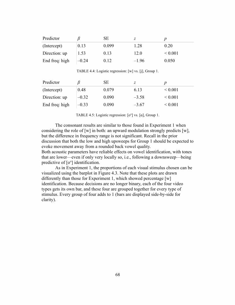
Predictor # SE z p(Intercept) 0.13 0.099 1.28 0.20Direction: up 1.53 0.13 12.0 < 0.001End freq: high –0.24 0.12 –1.96 0.050

TABLE 4.4: Logistic regression: [w] vs. [j], Group 1.

Predictor # SE z p(Intercept) 0.48 0.079 6.13 < 0.001Direction: up –0.32 0.090 –3.58 < 0.001End freq: high –0.33 0.090 –3.67 < 0.001

TABLE 4.5: Logistic regression: [o)] vs. [!], Group 1.

The consonant results are similar to those found in Experiment 1 when considering the role of [w] in both: an upward modulation strongly predicts [w], but the difference in frequency range is not significant. Recall in the prior discussion that both the low and high upsweeps for Group 1 should be expected to evoke movement away from a rounded back vowel quality.Both acoustic parameters have reliable effects on vowel identification, with tones that are lower—even if only very locally so, i.e., following a downsweep—being predictive of [o)] identification.

As in Experiment 1, the proportions of each visual stimulus chosen can be visualized using the barplot in Figure 4.3. Note that these plots are drawn differently than those for Experiment 1, which showed percentage [w] identification. Because decisions are no longer binary, each of the four video types gets its own bar, and these four are grouped together for every type of stimulus. Every group of four adds to 1 (bars are displayed side-by-side for clarity).

68

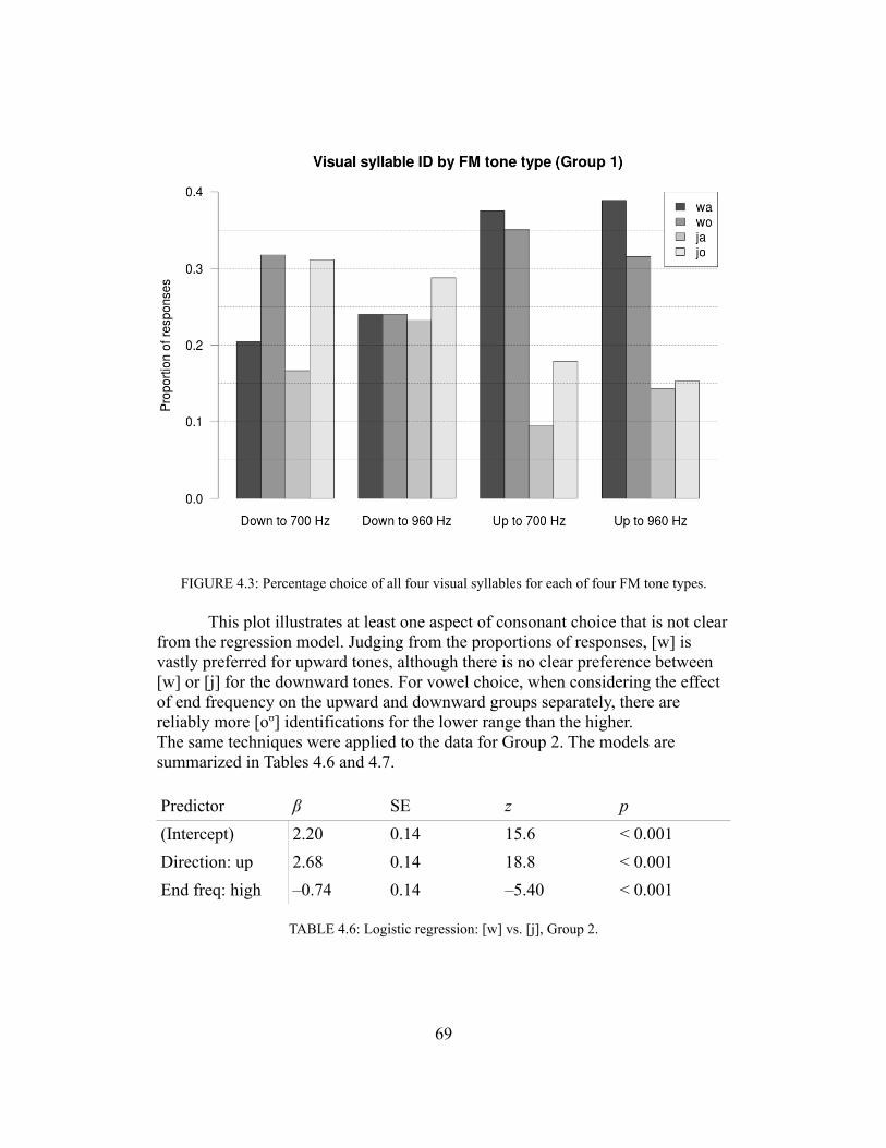
FIGURE 4.3: Percentage choice of all four visual syllables for each of four FM tone types.

This plot illustrates at least one aspect of consonant choice that is not clear from the regression model. Judging from the proportions of responses, [w] is vastly preferred for upward tones, although there is no clear preference between [w] or [j] for the downward tones. For vowel choice, when considering the effect of end frequency on the upward and downward groups separately, there are reliably more [o)] identifications for the lower range than the higher.The same techniques were applied to the data for Group 2. The models are summarized in Tables 4.6 and 4.7.

Predictor # SE z p(Intercept) 2.20 0.14 15.6 < 0.001Direction: up 2.68 0.14 18.8 < 0.001End freq: high –0.74 0.14 –5.40 < 0.001

TABLE 4.6: Logistic regression: [w] vs. [j], Group 2.

69

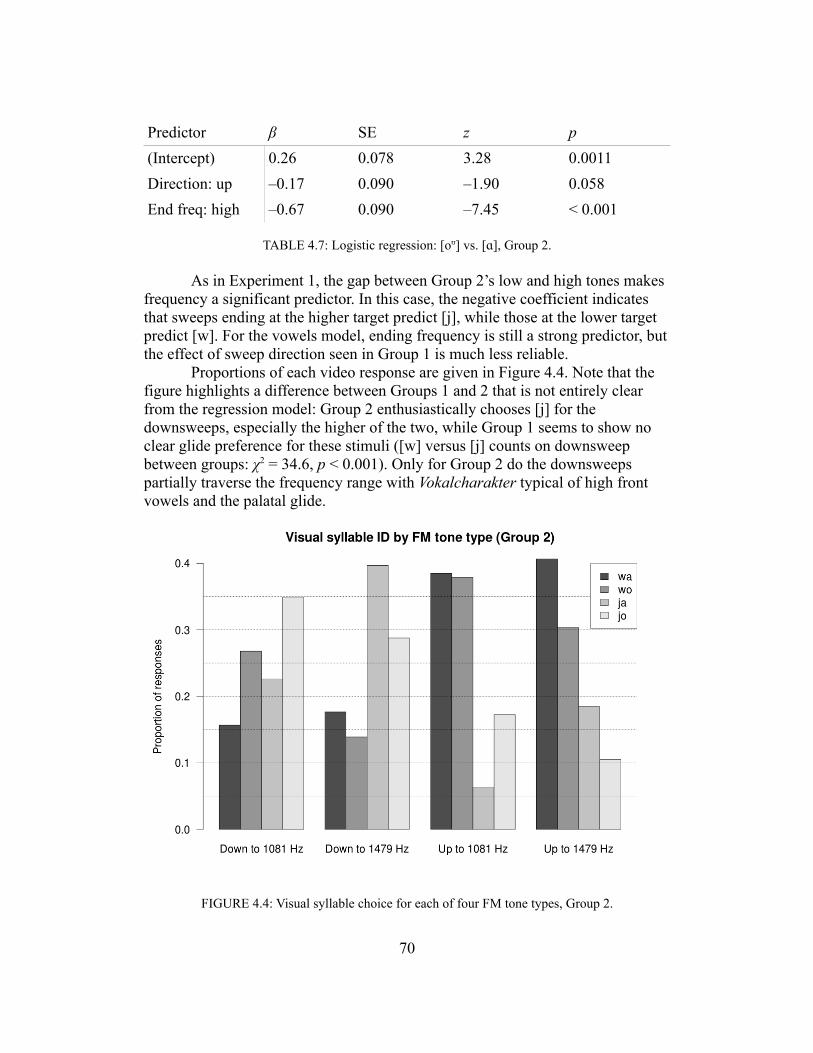
Predictor # SE z p(Intercept) 0.26 0.078 3.28 0.0011Direction: up –0.17 0.090 –1.90 0.058End freq: high –0.67 0.090 –7.45 < 0.001

TABLE 4.7: Logistic regression: [o)] vs. [!], Group 2.

As in Experiment 1, the gap between Group 2’s low and high tones makes frequency a significant predictor. In this case, the negative coefficient indicates that sweeps ending at the higher target predict [j], while those at the lower target predict [w]. For the vowels model, ending frequency is still a strong predictor, but the effect of sweep direction seen in Group 1 is much less reliable.

Proportions of each video response are given in Figure 4.4. Note that the figure highlights a difference between Groups 1 and 2 that is not entirely clear from the regression model: Group 2 enthusiastically chooses [j] for the downsweeps, especially the higher of the two, while Group 1 seems to show no clear glide preference for these stimuli ([w] versus [j] counts on downsweep between groups: %2 = 34.6, p < 0.001). Only for Group 2 do the downsweeps partially traverse the frequency range with Vokalcharakter typical of high front vowels and the palatal glide.

FIGURE 4.4: Visual syllable choice for each of four FM tone types, Group 2.

70

Discussion

Whereas Experiment 1 tested the suitability of FM tones to a glide versus a stop, including the effect of modulation rate, this one asked subjects to choose between sounds with different spectral but identical temporal characteristics. When varying the direction and absolute frequency of the tone sweep, clear associations between tones and glides emerged. Frequency range only mattered for glide identification in Group 2, who saw sweeps starting as high as 2500 Hz, well within the range found to evoke [i]. Group 1’s highest downsweep started at 1664 Hz, which is not a particularly good match for the semivowel [j] suggested by the visual, and results bore this out. Overall, the effects of sweep direction and range for semivowel selection are entirely consistent with the TEVs documented in previous work, and the present results show that these associations can be straightforwardly generalized to temporally modulated stimuli.Vowel choice also seemed to depend on aspects of the sweep, which was not concurrent with the visual vowel, indicating that identification is influenced by temporally proximal tones. I will return to this aspect of the results in the general discussion; before doing so, it is helpful to consider the simple case of vowel identification when no FM is present, which was measured in Experiment 2B.

Experiment 2B

For this short condition, audio stimuli differed from Experiment 2 in that the tones were not modulated in frequency. Stimuli were generated using the same method but with starting and ending frequencies being equivalent. All other aspects of the stimuli were the same. With duration and direction both rendered irrelevant, only two tone types, high and low, were available to each group. All possible combinations of one tone and two videos were generated, and two repetitions of each trial were presented, for a total of 48 trials. Subjects completed this session quickly, in about 4 minutes.

Results

Because only a single auditory parameter was varied for these stimuli, full regression models were not generated, and chi-squared tests on the counts of responses were used to determine the significance of the effect. For both groups, steady tone frequency had a significant impact on the numbers of responses of each vowel (Group 1 %2 = 28.8, p < 0.001; Group 2 %2 = 18.2, p < 0.001), but not on consonant responses (%2 = 1.52, p = 0.22; %2 = 0.02, p = 0.88). Response counts can be visualized similarly to Experiment 2 and are shown in Figures 4.5 and 4.6.

71

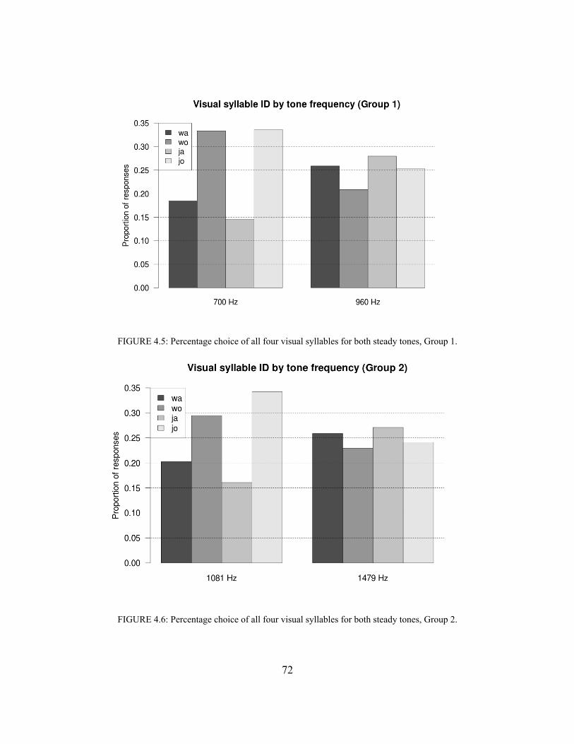
FIGURE 4.5: Percentage choice of all four visual syllables for both steady tones, Group 1.

FIGURE 4.6: Percentage choice of all four visual syllables for both steady tones, Group 2.

72

The results from this condition are simpler to interpret: when asked to choose both a vowel and consonant but are given only a simple tone, listeners extract a vowel percept before a glide percept. There is no evidence that either glide is evoked when FM is not present. As is consistent with prior research, when only two tone types are heard in the same block, [o)] is a more popular choice for the lower of the two.

An interesting difference does emerge between the two groups for this condition. Both show similar identification patterns between their respective high and low tones, with [o)] weakly preferred for the lower tone and no clear preference for the higher tone. What is of interest here is the fact that the low tone for Group 2 is just slightly higher than the high tone for Group 1, yet the pattern of behavior seems relative to the other tone heard in the same block. Presenting two stimulus types in the same block has been found to exaggerate effects of their differences (Johnson, 1990); in the context of this experiment, the observed adaptation to other stimuli in the block may follow from long-term auditory adaptation to statistical properties of frequency, as demonstrated by Holt (2005).

General discussion

The experiments in this study demonstrate that listeners can extract dynamic spectral cues from a minimally spectral dynamic stimulus—an FM tone. Observations of Vokalcharakter and the frequency ranges typically associated with various vowels can be cleanly generalized to semivowels, at modulation rates similar to speech. This extension is consistent with the view that the tone-vowel association is due to the same mechanisms that process speech. Although single FM tones are certainly not intelligible as speech, under controlled circumstances they have clear associations with speech sounds. I further discuss three points here. First, I address the theoretical significance of nonspeech-as-speech processing. I then delve further into the effects of relative frequency on vowel identification noted in my experiments. Finally, I offer some perspectives on the spectral features likely to be at the root of tone-evoked speech.

Speech processing of tones

Why are tones receiving the speech treatment? Past research has illustrated many cases of unmistakably phonetic or linguistic processing being applied to nonspeech: language experience (Iverson et al., 2011); phonetic context effects (Finley, 2012); and even universal and language-specific phonology (Berent et al., 2010). More generally, there is ample evidence of top-down linguistic/phonetic influences upon auditory perception (e.g., Davis & Johnsrude, 2007). It is reasonable and economical to posit that these tones are processed as speech would be, and phonetic identification follows automatically. This processing is probably at least partially motivated by the fact that the tones are concurrent with visual

73

articulation, inducing the expectation of speech; there is behavioral and neuroimaging evidence that it is possible to control, by exploiting experience or expectation, whether auditory input is processed in a ‘speech mode’ (Repp, 1982; Remez et al., 2001; Liebenthal et al., 2003; Möttönen et al., 2006).Processing artificial nonspeech as speech could have, paradoxically, ecological motivations. Real-world listening conditions are virtually never ideal—reverberation, acoustic filtering, noise, etc. are all possible obstacles to intelligibility. Speech perception needs to remain robust to these destructive effects; it would not be well served by the exclusion of hypothetically degraded inputs. The identification functions of pure tones do differ from those of speech in at least one aspect: the lack of a clear categorical boundary between two phones. Although the tones evoke speech sounds, the cues are generally insufficient to make a firm judgment. This aspect of the data suggests that, although listeners eagerly interpret phonetics from any kind of auditory input, the system remains particularly flexible when that input only partially matches known speech patterns.

Relative effects on vowel

The experiments presented here agree with past work on the approximate frequency ranges associated with broad vowel quality categories. As mentioned, there are no sharp boundaries in identification—neither in prior work, in which there are large bands of overlap between adjacent tone-evoked vowels, nor here, where a particular vowel or glide is usually not overwhelmingly chosen over the other option. The vagueness of the boundary suggests that it may be malleable, but no previous study has attempted to induce boundary shifts for these kinds of stimuli. Although that was not the stated intent of these experiments, I did find that vowel identification depended on both the frequency of the vowel-synced tone and the direction (and thus frequency range) of the preceding sweep. The sweep had minimal temporal overlap with the visual vowel, yet vowel preference showed a clear effect of direction: the vowel [o)] was more common when the vowel-synced portion was low in frequency relative to the consonant portion. Though reliable Vokalcharakter boundaries are difficult to measure, there is evidence here that the boundaries can be shifted by context.

The simple nature of the shift in this case—tones are modulated either up or down, with frequency change and rate held constant—makes it difficult to distinguish whether the boundary shift is best explained as phonetic or auditory in nature. If the effect is phonetic, the explanation would lie in compensating for the preceding glide, which would putatively move the vowel either forward or back. Consider these same experiments but with speech stimuli: nearly this same condition, ambiguous vowels in [w-w] or [j-j] contexts, was found by Lindblom and Studdert-Kennedy (1967) to induce compensatory phonetic effects. On the other hand, the effect could be considered purely auditory, as would be predicted

74

by the framework of spectral contrast (Lotto et al., 1997; Lotto and Kluender, 1998). Under this view, the spectral distance between points of high energy would perceptually exaggerated using cognitively general contrast mechanisms. The phonetic and auditory viewpoints make equivalent predictions for the simple case demonstrated here, and neither should be disregarded as a possible explanation.

Spectral features of tone-evoked speech

Finally, I would like to return to the question of exactly what it is about pure tones that makes them evocative of certain vowels. A naïve approach of matching the tone to vocal tract resonances actually finds striking parity between tone and F2 frequency. (It could also be said, for the back and low vowels, that the tone corresponds to the single spectral bump created by the first two formants.) However, an explanation of Vokalcharakter that rests only on F2 is problematic because it does not account for the predominance of low vowels, as opposed to mid or high central vowels, at around 1 kHz. Note that Fant (1973) shows very little identification of tones in this frequency range as the Swedish high central vowel, whereas an account relying on F2 only would predict this vowel would be as popular a choice as [!]. The Swedish data reinforce that we need to know not only where the vowels fall along the continuum, but also which vowels are most strongly evoked. For English, these vowels do appear to be those that have a somewhat band-limited characteristic: [u] and [o] are largely devoid of high frequencies; [!], slightly less so, but the high F1 and low F2 do leave significant gaps outside of a narrow mid-frequency band; [i], excepting its very low F1, is essentially high-pass, as is [y]. Although none of these vowels are exactly narrowband, all feature broad bands of very low spectral energy near their characteristic peaks. Tone spectra exhibit this same property to an extreme degree. Again, identification of filtered vowels bears out the same predictions: when introducing spectral zeros through filtering, misidentification tends to favor [i] for very high-pass sounds, and back rounded vowels for very low-pass sounds (Lehiste & Peterson, 1959).

That these spectral zeros are a property that is clearly shared between tones and the vowels they commonly evoke suggests that they are important perceptual cues. As another piece of evidence, consider that recognition accuracy of spectrally gapped speech can be enhanced by adding noise in the empty bands (Shriberg, 1992; Warren et al., 1997; Bashford et al., 2005; McDermott & Oxenham, 2008; Carlyon et al., 2002). If the filtering of speech creates artificial zero cues that listeners attempt to use, added noise effectively removes these spurious cues and forces the listener to ignore potential cues from those bands. It also creates a much more ecologically plausible stimulus, as natural background noise is much more common and plausible than natural sharp bandpass filters. The phonetic inference necessary in noise might be cast as a missing data problem, with an ideal approach perhaps similar in spirit to that of Cooke et al.

75

(2001), who apply noise estimation and missing data approaches (imputation) to automated speech recognition.

The tone-evoked speech results suggest that a model of speech sound recognition considering only poles in the vocal tract’s transfer function—i.e., formants—is insufficient to predict how these stimuli will be classified. Although formant frequencies constitute a useful, low-dimensional representation of speech acoustics, competing models that take the entire spectrum into account have been successful as well, and are more plausible given our knowledge of psychoacoustics and auditory physiology (Bladon & Lindblom, 1981; Bladon, 1982; Ito et al., 2001; Molis, 2005). This is a major debate in the literature and should take into account results from nonspeech stimuli. Even cases of auditory stimuli generating a very subtle speech percept, as with Vokalcharakter, should not be considered irrelevant to speech perception; on the contrary, these very controlled stimuli offer a unique perspective on how to reverse-engineer the cognitive machinery.

Human speech processing allows a wide variety of possible inputs, and models of spectral recognition need to make correct predictions for any stimulus with speech associations. The present work has demonstrated the possibility for stimuli of minimal spectral complexity to evoke dynamic speech and related this behavior directly to their spectral properties. Other findings of the experiments, such as the relative effects on vowel association over the length of a tone or an entire experimental block, can be related to known auditory and phonetic phenomena. I also suggested a research direction towards an explanation for tonal Vokalcharakter and noted ways in which current models of spectral perception fall short. These findings should reinforce the usefulness of nonspeech work in phonetics and highlight the extraordinary ability of human listeners to find speech in difficult conditions, including the absence of speech altogether.

76

Part IIIModels of phonetic spectral recognition

77

Chapter 5Models of spectral perception

The experimental work covered in the previous chapters speaks to the generality of speech perception given diverse auditory inputs. Certain nonspeech sounds have demonstrable phonetic value for listeners, and results suggest that the evoked phonetics can be explained by the acoustic similarities between learned speech categories and the nonspeech stimulus. Examining speech-nonspeech perception allows a unique approach to reverse-engineer how listeners process speech. If these responses are in fact rooted in the same type of analysis ordinarily performed for speech inputs, as is suggested by these similarities, then they should also be predicted by a faithful model of speech perception. Therefore, a way to incorporate speech-nonspeech effects into perceptual theory is to work towards modeling phonetic perception in a way that is consistent with human responses to both speech and nonspeech.

The experiments thus far have shown both temporal and spectral aspects of speech-nonspeech processing. For the most part, the acoustic speech-nonspeech parity has been spectral in nature, and I focus exclusively on this domain here. In this chapter I review some of the existing models of spectral perception and the historical development of various types of models. This review lays the ground for Chapter 6, in which I present new computational experiments on spectral recognition that address the question of how these models would fare on the nonspeech stimuli seen previously in the dissertation.

Background

The modeling of spectral recognition has generally been framed as vowel recognition, as vowels are reliable targets for spectral processing due to their high audibility, linguistic importance, and rich harmonic structure. Early characterizations of vowels cast them in terms of formants, which have direct relevance to their articulation. As a faithful model of perception, however, representations based on the acoustics of production are problematic for a number of reasons. Alternative proposals have considered the whole spectrum or other derived features. In this section, I present a historically oriented review of the modeling of spectral vowel perception, followed by a discussion of how progress towards this goal can impact our understanding of speech-nonspeech phenomena.

Of tangential interest to the endeavor of modeling human perception is the development of practical engineering models for mimicking human performance. I do not devote much discussion to these, although I will mention here two examples that I find representative of the interesting crossover between fields: perceptual linear prediction (PLP; Hermansky, 1990), which takes psychoacoustic findings into account to enhance spectral processing of speech; and Zahorian and

78

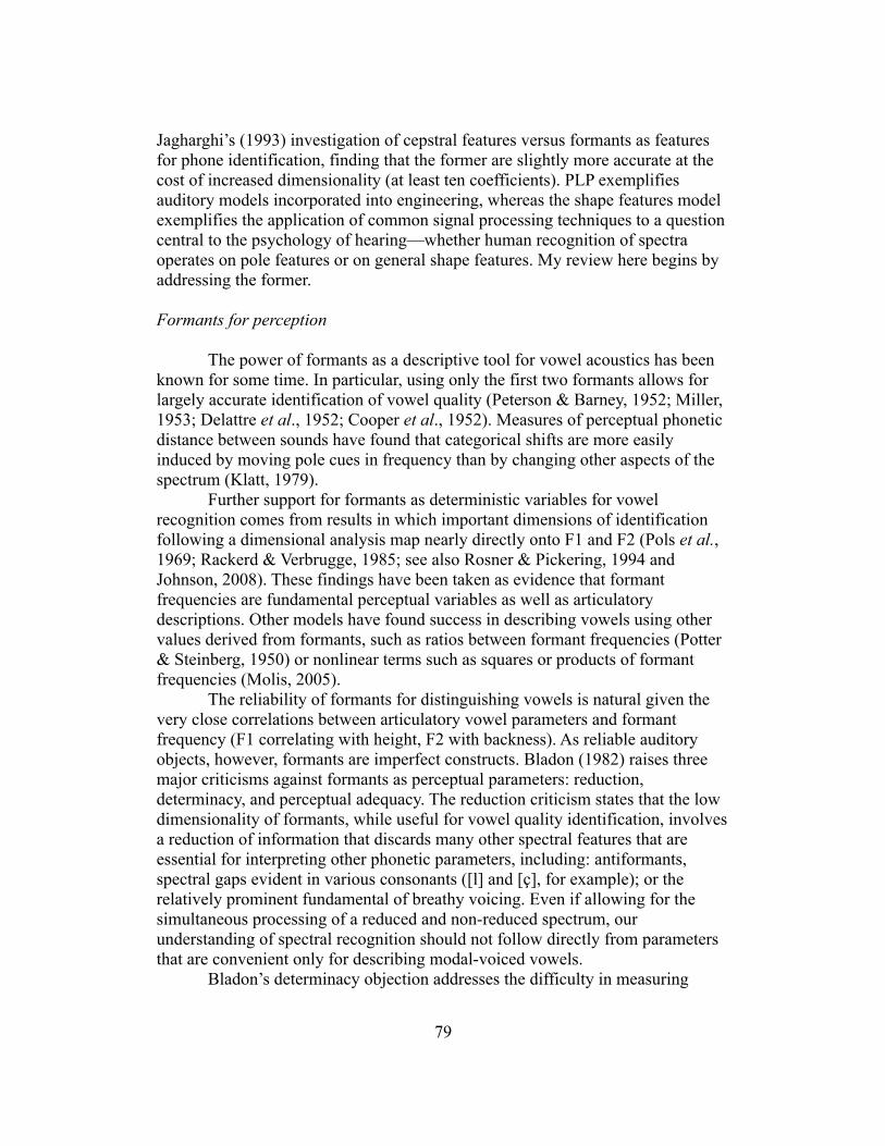
Jagharghi’s (1993) investigation of cepstral features versus formants as features for phone identification, finding that the former are slightly more accurate at the cost of increased dimensionality (at least ten coefficients). PLP exemplifies auditory models incorporated into engineering, whereas the shape features model exemplifies the application of common signal processing techniques to a question central to the psychology of hearing—whether human recognition of spectra operates on pole features or on general shape features. My review here begins by addressing the former.

Formants for perception

The power of formants as a descriptive tool for vowel acoustics has been known for some time. In particular, using only the first two formants allows for largely accurate identification of vowel quality (Peterson & Barney, 1952; Miller, 1953; Delattre et al., 1952; Cooper et al., 1952). Measures of perceptual phonetic distance between sounds have found that categorical shifts are more easily induced by moving pole cues in frequency than by changing other aspects of the spectrum (Klatt, 1979).

Further support for formants as deterministic variables for vowel recognition comes from results in which important dimensions of identification following a dimensional analysis map nearly directly onto F1 and F2 (Pols et al., 1969; Rackerd & Verbrugge, 1985; see also Rosner & Pickering, 1994 and Johnson, 2008). These findings have been taken as evidence that formant frequencies are fundamental perceptual variables as well as articulatory descriptions. Other models have found success in describing vowels using other values derived from formants, such as ratios between formant frequencies (Potter & Steinberg, 1950) or nonlinear terms such as squares or products of formant frequencies (Molis, 2005).

The reliability of formants for distinguishing vowels is natural given the very close correlations between articulatory vowel parameters and formant frequency (F1 correlating with height, F2 with backness). As reliable auditory objects, however, formants are imperfect constructs. Bladon (1982) raises three major criticisms against formants as perceptual parameters: reduction, determinacy, and perceptual adequacy. The reduction criticism states that the low dimensionality of formants, while useful for vowel quality identification, involves a reduction of information that discards many other spectral features that are essential for interpreting other phonetic parameters, including: antiformants, spectral gaps evident in various consonants ([l] and [ç], for example); or the relatively prominent fundamental of breathy voicing. Even if allowing for the simultaneous processing of a reduced and non-reduced spectrum, our understanding of spectral recognition should not follow directly from parameters that are convenient only for describing modal-voiced vowels.

Bladon’s determinacy objection addresses the difficulty in measuring

79

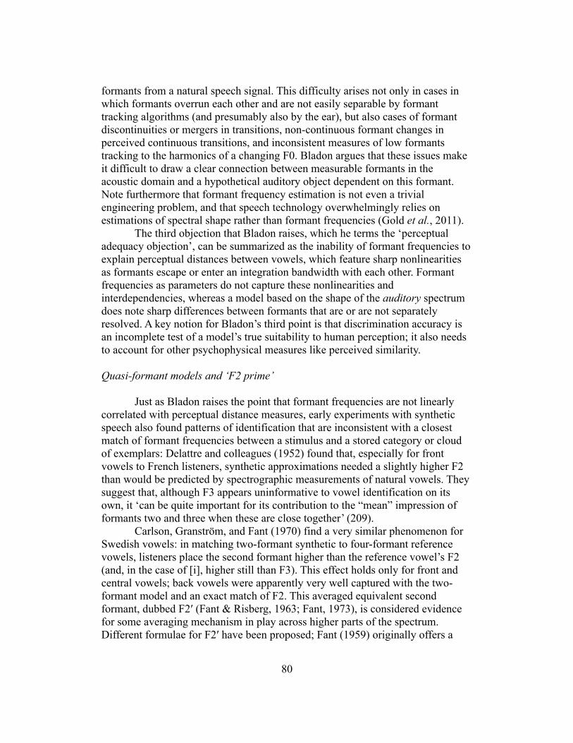
formants from a natural speech signal. This difficulty arises not only in cases in which formants overrun each other and are not easily separable by formant tracking algorithms (and presumably also by the ear), but also cases of formant discontinuities or mergers in transitions, non-continuous formant changes in perceived continuous transitions, and inconsistent measures of low formants tracking to the harmonics of a changing F0. Bladon argues that these issues make it difficult to draw a clear connection between measurable formants in the acoustic domain and a hypothetical auditory object dependent on this formant. Note furthermore that formant frequency estimation is not even a trivial engineering problem, and that speech technology overwhelmingly relies on estimations of spectral shape rather than formant frequencies (Gold et al., 2011).

The third objection that Bladon raises, which he terms the ‘perceptual adequacy objection’, can be summarized as the inability of formant frequencies to explain perceptual distances between vowels, which feature sharp nonlinearities as formants escape or enter an integration bandwidth with each other. Formant frequencies as parameters do not capture these nonlinearities and interdependencies, whereas a model based on the shape of the auditory spectrum does note sharp differences between formants that are or are not separately resolved. A key notion for Bladon’s third point is that discrimination accuracy is an incomplete test of a model’s true suitability to human perception; it also needs to account for other psychophysical measures like perceived similarity.

Quasi-formant models and ‘F2 prime’

Just as Bladon raises the point that formant frequencies are not linearly correlated with perceptual distance measures, early experiments with synthetic speech also found patterns of identification that are inconsistent with a closest match of formant frequencies between a stimulus and a stored category or cloud of exemplars: Delattre and colleagues (1952) found that, especially for front vowels to French listeners, synthetic approximations needed a slightly higher F2 than would be predicted by spectrographic measurements of natural vowels. They suggest that, although F3 appears uninformative to vowel identification on its own, it ‘can be quite important for its contribution to the “mean” impression of formants two and three when these are close together’ (209).

Carlson, Granström, and Fant (1970) find a very similar phenomenon for Swedish vowels: in matching two-formant synthetic to four-formant reference vowels, listeners place the second formant higher than the reference vowel’s F2 (and, in the case of [i], higher still than F3). This effect holds only for front and central vowels; back vowels were apparently very well captured with the two-formant model and an exact match of F2. This averaged equivalent second formant, dubbed F2* (Fant & Risberg, 1963; Fant, 1973), is considered evidence for some averaging mechanism in play across higher parts of the spectrum. Different formulae for F2* have been proposed; Fant (1959) originally offers a

80

strategy depending on the first three formant frequencies only, but later proposals also incorporate information about formant amplitudes and even formants beyond F3 (e.g., Bladon & Fant, 1978).

Work along these lines has also considered a ‘center of gravity’ hypothesis for the formants determining F2*: the perceptually best single-formant replacement for two higher formants depends not only upon their frequencies but also upon the ratio of their amplitudes (Chistovich & Lublinskaya, 1979), with F2* attracted towards the center of gravity between them. Critically, however, this dependence vanishes once a certain threshold in formant differences—about 3 to 3.5 Bark—is reached. The discovery of this window of integration was hugely influential to thinking about the perceptual nature of formants: for example, Bladon (1983) demonstrates that incorporating this finding dramatically improves the performance of ‘two-bump’ models of vowel spectra; Syrdal and Gopal (1986) motivate a model of vowel recognition based largely on 3-Bark separations between F0 and F1 and between F2 and F3.

There is evidence that the reduction of higher formants to a single center of gravity is too simplistic to account for vowel identification. Assmann (1991) shows that changes in F2 amplitude do not correlate with shifts in identification that the formant center of gravity hypothesis would predict. Nearey and Kiefte (2003) investigate the suitability of two- or three-dimensional representations of vowel quality in an artificial neural network with either two or three units in the hidden layer, finding that two dimensions leads to too severe a bottleneck to accurately represent phonetic distinctions. Although Bladon’s (1982) criticism of the perceptual adequacy of formants is addressed somewhat by these two-bump models, the criticism of reduction remains valid.

Whole spectral shape

Other approaches, in contrast to formant models or their derivatives, consider the spectral shape in its entirety rather than seeking a reduction in parameters via tracking pole features. A fundamental problem in motivating a whole-spectrum model over a formant model, or vice versa, is the strong parity between the spectrum and formant frequencies and amplitudes: as poles in the vocal tract transfer function, formants are the major acoustic determinants of spectral shape, and any other features used to represent spectral shape are also going to be encoding formant information (Johnson, 2005; Broad & Clermont, 1989).

The distinction between poles and spectral shape here is further muddied by the possibility that cues better suited to either approach might trade in importance. That is, cues that are better described as spectral peaks may be favored in certain contexts (the specifics of which encompass type and level of background noise, type of speech sound, age or gender of speaker), and off-peak, shape-based cues may be favored in others. Evidence that this may be the case

81

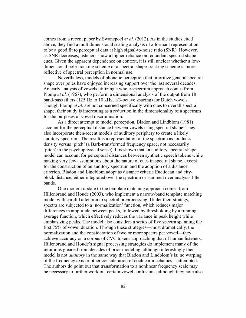
comes from a recent paper by Swanepoel et al. (2012). As in the studies cited above, they find a multidimensional scaling analysis of a formant representation to be a good fit to perceptual data at high signal-to-noise ratio (SNR). However, as SNR decreases, listeners show a higher reliance on redundant spectral shape cues. Given the apparent dependence on context, it is still unclear whether a low-dimensional pole-tracking scheme or a spectral shape-tracking scheme is more reflective of spectral perception in normal use.

Nevertheless, models of phonetic perception that prioritize general spectral shape over poles have enjoyed increasing support over the last several decades. An early analysis of vowels utilizing a whole-spectrum approach comes from Plomp et al. (1967), who perform a dimensional analysis of the output from 18 band-pass filters (125 Hz to 10 kHz, 1/3-octave spacing) for Dutch vowels. Though Plomp et al. are not concerned specifically with cues to overall spectral shape, their study is interesting as a reduction in the dimensionality of a spectrum for the purposes of vowel discrimination.

As a direct attempt to model perception, Bladon and Lindblom (1981) account for the perceptual distance between vowels using spectral shape. They also incorporate then-recent models of auditory periphery to create a likely auditory spectrum. The result is a representation of the spectrum as loudness density versus ‘pitch’ (a Bark-transformed frequency space, not necessarily ‘pitch’ in the psychophysical sense). It is shown that an auditory spectral-shape model can account for perceptual distances between synthetic speech tokens while making very few assumptions about the nature of cues in spectral shape, except for the construction of an auditory spectrum and the adoption of a distance criterion. Bladon and Lindblom adopt as distance criteria Euclidean and city-block distance, either integrated over the spectrum or summed over analysis filter bands.

One modern update to the template matching approach comes from Hillenbrand and Houde (2003), who implement a narrow-band template matching model with careful attention to spectral preprocessing. Under their strategy, spectra are subjected to a ‘normalization’ function, which reduces major differences in amplitude between peaks, followed by thresholding by a running average function, which effectively reduces the variance in peak height while emphasizing peaks. The model also considers a series of five spectra spanning the first 75% of vowel duration. Through these strategies—most dramatically, the normalization and the consideration of two or more spectra per vowel—they achieve accuracy on a corpus of CVC tokens approaching that of human listeners. Hillenbrand and Houde’s signal processing strategies do implement many of the intuitions gleaned from decades of prior modeling, although interestingly their model is not auditory in the same way that Bladon and Lindblom’s is; no warping of the frequency axis or other consideration of cochlear mechanics is attempted. The authors do point out that transformation to a nonlinear frequency scale may be necessary to further work out certain vowel confusions, although they note also

82

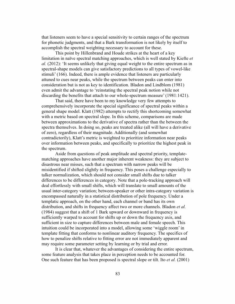
that listeners seem to have a special sensitivity to certain ranges of the spectrum for phonetic judgments, and that a Bark transformation is not likely by itself to accomplish the spectral weighting necessary to account for these.

This point by Hillenbrand and Houde strikes at the heart of a key limitation in naïve spectral matching approaches, which is well stated by Kiefte et al. (2012): ‘It seems unlikely that giving equal weight to the entire spectrum as in spectral-shape models can give satisfactory predictions to all types of vowel-like stimuli’ (166). Indeed, there is ample evidence that listeners are particularly attuned to cues near peaks, while the spectrum between peaks can enter into consideration but is not as key to identification. Bladon and Lindblom (1981) even admit the advantage to ‘reinstating the spectral peak notion while not discarding the benefits that attach to our whole-spectrum measure’ (1981:1421).

That said, there have been to my knowledge very few attempts to comprehensively incorporate the special significance of spectral peaks within a general shape model. Klatt (1982) attempts to rectify this shortcoming somewhat with a metric based on spectral slope. In this scheme, comparisons are made between approximations to the derivative of spectra rather than the between the spectra themselves. In doing so, peaks are treated alike (all will have a derivative of zero), regardless of their magnitude. Additionally (and somewhat contradictorily), Klatt’s metric is weighted to prioritize information near peaks over information between peaks, and specifically to prioritize the highest peak in the spectrum.

Aside from questions of peak amplitude and spectral priority, template-matching approaches have another major inherent weakness: they are subject to disastrous near misses, such that a spectrum with narrow peaks will be misidentified if shifted slightly in frequency. This poses a challenge especially to talker normalization, which should not consider small shifts due to talker differences to be differences in category. Note that a pole-tracking approach will deal effortlessly with small shifts, which will translate to small amounts of the usual inter-category variation; between-speaker or other intra-category variation is encompassed naturally in a statistical distribution of pole frequency. Under a templatic approach, on the other hand, each channel or band has its own distribution, and shifts in frequency affect two or more channels. Bladon et al. (1984) suggest that a shift of 1 Bark upward or downward in frequency is sufficiently warped to account for shifts up or down the frequency axis, and sufficient in size to capture differences between male and female speech. This intuition could be incorporated into a model, allowing some ‘wiggle room’ in template fitting that conforms to nonlinear auditory frequency. The specifics of how to penalize shifts relative to fitting error are not immediately apparent and may require some parameter setting by learning or by trial and error.

It is clear that, whatever the advantages of considering the entire spectrum, some feature analysis that takes place in perception needs to be accounted for. One such feature that has been proposed is spectral slope or tilt. Ito et al. (2001)

83

demonstrate that the slope of the spectrum as defined by the amplitude ratio of F1 and F2 could drive judgments of vowel quality. Even more surprising, complete excising of certain formants had less of an effect on quality than altering spectral tilt. Crucially, Ito et al. maintain frequency separation between formants of greater than the 3.5 Bark hypothesized to be necessary for formants to merge under the center of gravity hypothesis, indicating that tilt operates across the spectrum.

As a single parameter for differentiating broad classes of spectral shapes, tilt is appealing for its reductive power. On the other hand, its simplicity makes it difficult to define its specific role in vowel identification, not to mention fluent speech. Moreover, there is evidence from Kiefte and Kluender (2005) that tilt loses importance for categorizing non-steady-state sounds, for which listeners rely more heavily on pole frequency cues: although tilt is a major predictor of /i/ versus /u/ judgments, judgments of diphthongs as /ai/ or /au/ were driven entirely by their formant frequencies. The authors suggest an explanation rooted in inference performed by listeners: spectrotemporal change is the characteristic salient property of natural speech, and unlikely to be the result of external factors, whereas gross measures like tilt could have origins in the acoustics of the transmission channel. Modulation cues, when available, trump unchanging spectral shape cues, as the former are less likely to have a non-phonetic source.

A more comprehensive picture is filled out in a later study by Kiefte and Kluender (2008), in which the authors note that features absent from preceding speech context are more predictive of identification patterns: when context was filtered with a single pole or zero to match a given tilt, recognition of the following vowel was dominated by F2 frequency; but when a resonance filter was applied to context, tilt determined vowel quality. Which cue is relied upon depends on perceived properties of the environment or channel, and human listeners are very good at the scene analysis necessary to separate channel from source. The question of cue reliability comes up similarly in a study by Alexander and Kluender (2008) demonstrating that listeners with hearing impairment are less likely than normal hearing listeners to reweight tilt and F2 cues to stop identity, presumably due to hearing impairment’s effect on spectral peak resolution. These results, taken together with Kiefte and Kluender’s 2005 study, suggest not that perception is driven by default by one type of cue or the other, but that listeners classify sounds by identifying which acoustic properties of the stimulus are reliable—that is, discernible from those inherent to the combined effects of the acoustic or auditory channels.

A final note on the distinction between pole cues and shape cues, especially as concerns the auditory representation of these cues: the above results may also suggest that pole cues are more reliable for tracking rapid change, whereas more complex shape representations are less straightforwardly extended across time. Detection of spectral shape can be explained with some adequacy through cochlear tonotopy, whereas spectrotemporal auditory features rely on representations that may not be available pre-cortically. The differences noted by

84

Kiefte and Kluender (2005) may arise from differences in physiological analysis strategies applied to stimuli having different modulation rates.

Evaluating model accuracy

Gauging the relative effectiveness of different modeling strategies across these studies is virtually impossible because of differences in the speech data used. A fairly comprehensive attempt to test several strategies on a level playing field comes from Molis (2005), who evaluates various formant- and spectrum-based representations and their fit to human judgments on 54 synthetic vowels that varied in F2 and F3. Molis considers various features derived from the vowels as inputs to logistic regression, including: formant frequencies and amplitudes; squares and products of F2 and F3; PLP cepstral coefficients (Hermansky, 1990); auditory excitation patterns, reduced to the first six principal components; and the slope of the excitation patterns (similar to Klatt’s [1982] model discussed above), reduced to the first ten principal components. She finds that the nonlinear formant frequencies model and the excitation pattern model are the best fits for human identification, the slope metric a particularly poor fit, and the PLP coefficients somewhere in between. While formants do perform slightly better than the spectral shape model, Molis cautions against the consideration only of formants: there are other phenomena, as discussed above, that they fail to capture. And the exclusion of F1 as a variable for the vowels in Molis’s study leaves open the question of how formant models or spectral shape models would handle the certainly meaningful shifts in vowel identification resulting from changes in F1.

General discussion

Despite early observations that important speech contrasts could be boiled down to a few resonances in a spectrum, and despite quintessential work in describing speech production in terms of acoustic resonances, numerous studies over the last half century have cast doubt upon the importance of formants to perception. In their place, notions of spectral perception that consider the entire spectral template itself have been gradually gaining in acceptance and sophistication. Molis’s (2005) results capture what is, I think, still essentially the status of this line of research: models of phonetic spectral perception can be made very effective, with performance closely matching that of human listeners, by careful tuning of the features, regardless of the nature of those features. If there is little to distinguish a formant model from a spectral shape model in terms of their fit to perceptual data, then a more important consideration might be the psychophysiological plausibility of the processing strategy.

Formants, as they are currently defined for the acoustic analysis of speech, are unlikely to have direct perceptual correlates. For relatively steady spectra,

85

listeners have no empirical way to differentiate between one formant and two overlapping formants; furthermore, the auditory bandwidth for resolution of separate spectral prominences is especially wide—wider than peripheral frequency resolution would predict, and certainly wider than can be visually resolved from the acoustic spectrum. Other experimental evidence is even more problematic for the notion of spectral peaks as perceptual targets—for example, the finding that they can be removed entirely under certain circumstances as long as spectral tilt remains relatively unaffected (Ito et al., 2001). In short, formants cannot plausibly be considered the exclusive currency of spectral perception.

Of course, formant frequencies and amplitudes are such useful, intuitive, and low-dimensional descriptors of articulation and determinants of spectral shape that they maintain a strong presence in auditory phonetics research. On the other side of the coin, signal processing schemes such as cepstra are famously reliable as measurements of spectral shape for engineering purposes (assuming a clean signal). And indeed, these capture many aspects of shape with low dimensionality and have proven useful for decades, even for modeling perceptual judgments (Zahorian and Jagharghi, 1993). However, a Fourier-like analysis of the spectrum, as required for a cepstral analysis, does not seem well supported by any hardware of the auditory system. (Cepstra are also a poor model of human judgments because they break down in noisy conditions and are sensitive to nonlocal disruptions of the signal; see the discussion of Chapter 6.)

Interestingly, it can be pointed out that Molis’s own whole-spectrum model relies on principal components analysis (PCA) to pick out appropriate features for regression. Although neuronal circuits are capable of logical operations and pooling information from multiple inputs, it is not altogether clear that a biological equivalent to PCA exists for something like a spectrum. Higher-level cortical areas may be tuned specifically to certain tonotopical configurations or combinations, but that does not necessarily support a very general dimensionality reduction strategy. All of this is not to say that Molis’s features are invalid, but it does suggest that the machinery of the classification algorithm is markedly different from the human strategy. The cognitive nature of the decision rule, and its psychological plausibility, are an entirely different question to the auditory features themselves.

If anything, whole-spectrum approaches, so long as they are cognizant of peripheral limitations and critical bands, are generally conservative, as they produce representations of sounds that could essentially be read directly off the auditory nerve. The numerous and complex stages of central audition are, in view of these simple template models, only necessary for parsing that spectral template and making comparisons to others. Certainly, an accurate model must make consideration of central abilities in a way that these simple models do not; however, from a certain point of view, central processes can only improve the processing of these templates.

This notion of plausibility to human perception brings up the question of

86

whether questions in this research agenda are even well posed. Put another way, the attempts over the last several decades to find faithful models necessarily rest on the assumption that there is a spectral recognition process to model. There are reasons to believe that the phonetic parsing of spectra is not an altogether relevant or informative question. One reason follows from the discussion of Kiefte and Kluender’s experiments, which show cues changing dramatically in importance given a signal with temporal dynamics or certain acoustic history before a target stimulus. If the nature of spectral recognition changes dramatically in certain contexts, then is there anything fundamental to say about purely spectral processing? Looking at how the context is altering a listener’s reception of spectral properties of the target may be more interesting and informative. Furthermore, what of the multiple and interacting levels of auditory perception—understanding acoustic properties of the source, of the channel, and of one’s own hearing? Specifically modeling phonetic spectral perception may be attempting to boil a complex problem down to components that cannot be effectively analyzed separately.

Perhaps the most devastating criticism of the approach taken by virtually all of the studies discussed in this chapter is that speech is not a spectral phenomenon. That is, speech depends on temporal events and spectrotemporal transitions, and known facts about perception are inconsistent with a simple model of speech as a constant sequence of spectra. Characterizations of salient auditory and phonetic objects need to be able to incorporate both spectral and temporal information; note that even auditory properties seemingly spectral in nature, such as timbre, might depend more fundamentally on distinctive spectrotemporal patterns (Elliott et al., 2013). Under this view, spectral processing is negligibly relevant, as it can account only for the special case of zero temporal modulation.

Needless to say, given that I have chosen to undertake this question, I do not see these criticisms as entirely fatal to its pursuit. The fact that many sonorant phones do involve noticeably different spectra, and that these spectra are more intrinsically tied to their phonetics than other acoustic variables such as level or F0, points at the very least to the necessity of capturing these differences. And even the assumption that spectral recognition is entirely divorced from temporal dynamics need not apply. Spectrotemporal changes probably do act to tune and stabilize spectral representations, either through a relative lack of change or through key changes that enable scene analysis by highlighting acoustic aspects of the signal versus those of competing signals or the transmission channel.

Indeed, just as bands in the spectrum are likely weighted for importance (through mechanisms not yet adequately understood), spectra themselves may be weighted for reliability or importance to lexical identification, and these weights determined by attending to the rates and types of spectrotemporal change. There is ample room for other aspects of spectral perception to be extended to spectrotemporal perception as well. Not least of these could be the importance of

87

gaps as cues, as already noted in Chapter 4: just as gaps in the spectrum can signal certain vowels, gaps in the auditory spectrogram can signal pauses, which may be interpreted as stop closures or prosodically important breaks. Note that, just as intelligibility improves when stopped bands are replaced with noise, the same occurs with temporally gapped speech, a phenomenon known as the picket fence effect (Miller & Licklider, 1950).

Conclusion

As the theory of spectral phonetic recognition currently stands, there is evidence for both the importance and the inadequacy of spectral poles. A claim that formants in speech production translate directly into perceptual objects is certainly flawed, or at least oversimplified, as seen by overwhelming evidence both for contrasts that do not depend on formant frequencies and for formants near in frequency failing to constitute perceptually separable cues. Nevertheless, spectral peaks undeniably constitute important anchors for phonetic identification, and a straightforward template-matching approach misses this observation.

To date, a satisfying union of these notions has not been adopted. The task faces at least two major complications: first, the extreme redundancy between pole- and shape-based representations, as seen from factor analyses of both; and second, the tradeoffs between qualitatively different cues in different experimental contexts. An ideal model of spectral recognition will have to capture the system’s flexibility while achieving human-like performance on a wide variety of data sets and for many different speech conditions. Additionally, such a model should be maximally compatible with auditory physiology, respecting cochlear mechanics and even central processing as much as possible. Certain very effective strategies for automated phonetic classification, such as cepstral analysis or PCA, rely on assumptions about auditory abilities that may not be psychophysically supported.

The next chapter presents further investigation of this question on new types of sounds. I test formant and spectral shape models on phones extracted from fluent speech, whereas most of the above strategies concern isolated vowels or syllables, as well as on nonspeech sounds. The success of one modeling strategy in both of these domains may indicate its superiority as a reflection of perceptual processing.

88

Chapter 6Testing models of spectral perception, speech and nonspeech

In this chapter I present experiments on the effectiveness of several types of spectral classifiers for speech and nonspeech. As reviewed in the previous chapter, numerous models of spectral recognition in human listeners have been proposed. The impetus to revisit this question here follows from the central theme of this thesis: listeners can hear nonspeech sounds as speech. Prior attempts to model spectral perception have not given consideration to how nonspeech sounds would be processed by a speech-centric model. An accurate psychological model of phonetic recognition should not only make relevant predictions about speech, but also mimic responses given by human listeners under speech-nonspeech processing. And ideally, such a model would also be consistent with the constraints on human auditory abilities. Peripheral auditory models are readily available and can be applied to partially ensure the auditory plausibility of a phonetic model.

In the experiments that follow, I evaluate a number of representations of spectra for classification, several of which are similar to those noted in the previous chapter. Models tested fall into two major classes: those based on the entire spectrum, and those based on formants. Formants, although not realistic auditory representations of speech, are descriptively adequate for many sounds and omnipresent in speech perception research. Another advantage to formants, from a practical or information theoretical perspective, is their low dimensionality: two to four formants capture most important vowel distinctions, and certain key features of consonants as well. It is far from evident how to reduce a spectrum to so few parameters without relying on pole cues.

For the purposes of this chapter, formants work well as features to a statistical classifier. Whole-spectrum sound identification, on the other hand, does not provide an obvious means of reducing the dimensionality of a spectrum. I provide two possible solutions: first, a perceptually plausible means of reducing dimensionality for spectral templates via critical bandwidths; and second, an alternative means of classifying spectral shape via a naïve minimum squared distance metric, which is less optimal than a discriminative classifier but better suited for high-dimensional data. The latter in particular makes very few modeling assumptions, except that optimum categorization minimizes distance to the category average. Both solutions and the nature of the features they generate are covered in detail below.

For the speech-nonspeech effects observed experimentally earlier in this dissertation, I have favored explanations having to do with the spectral similarities between these sounds and the phonetic categories they evoke. The model of phonetic recognition, then, should apply the same strategies when classifying

89

speech and nonspeech, without knowledge a priori of whether the input is speech. In concrete terms, the parameters of the model should be set according to speech inputs but applicable to nonspeech inputs. It is the nature of the features themselves that is up for investigation.

These experiments mostly operated on features derived from 1024-point fast Fourier transform (FFT) spectra of speech sounds. The assumption underlying feature generation is that there are human-interpretable spectral cues present in a window of that size. To confirm that this is the case, a task was devised for human listeners to categorize these sounds, and their performance evaluated similarly to the machines’. Note that a direct comparison between human and machine performance at this task would require many assumptions that are probably untenable (see the discussion at the end of this chapter). The purpose of the human experiment, then, is not to give a benchmark for classifier performance, but rather to confirm that the types of data used for classification do possess spectral cues that human listeners can pick up on.

Method

Data: speech

The acoustic data used for building and testing classifiers was taken from the DARPA TIMIT Acoustic-Phonetic Continuous Speech Corpus, which contains 6300 sentences spoken by 630 speakers of American English from various dialect regions. TIMIT provides manually transcribed speech along with phone boundaries. All sounds are sampled at 16 kHz. Speakers across the corpus differ in carefulness of pronunciation; however, all sentences feature plausible fluent speech with normal prosody, coarticulation, and phonetic reduction.

A total of 12 English phonemes were considered for this study: /i/, /e/, /æ/, /!/, /u/, /o/, /+/, /r/, /l/, /w/, /m/, and /n/, with corresponding common phonetic realizations of [i], [e(], [æ], [!], [&], [o)], [+], [,], [-], [w], [m] and [n]. Any lax vowels with a tense counterpart were excluded, as a major redundant cue in differentiating these is duration, and no consideration of duration was allowed for in this study. Also excluded were diphthongs that contained considerable changes in vowel quality: /"(/, /a)/, and /a(/. Additionally, non-velarized [l] tokens were not included, as they are generally very short in duration and presumably rely on temporal cues more than velarized [-]. Note also that /u/ and /w/ have major spectral differences, with the phonetic realization of what is conventionally written as /u/ being closer, in most cases, to [&] or even [y] in American English; /w/, on the other hand, has a spectrum closer to a true back [u]. The velar nasal /./ was not included because of common allophony with [n] and its lack of salience as a separate phoneme to many speakers.

Several hundred tokens of each phone were extracted automatically from the TIMIT corpus according to provided transcriptions and boundaries. No tokens

90

measured at shorter than 1500 samples (about 94 ms) were used, as these may have been severely phonetically reduced. Counts of each phone are provided in the appendix. Twenty tokens of each phone, 240 total, were selected at random to constitute the test set. Classifiers or human listeners were asked to identify each token as one of the 12 phones.

Signal processing for features

Many types of features were extracted from the speech data. Some were spectrally derived: magnitude spectra, cochlear excitation patterns, and a low-dimensional representation based on critical bandwidths. I first describe the specifications for generating these and then discuss formants and cepstral features.

For all phones, a 1024-point FFT (hamming windowed) was taken from the midpoint of the labeled token. Magnitude was kept, and phase discarded. One feature type was the magnitude spectrum itself, from points 6 to 205 (about 100 Hz to about 3200 Hz).

Spectra were also converted into representations of cochlear excitation patterns (EPs) using the method and formulae described by Moore and Glasberg (1983): estimated auditory filters with a roughly triangular shape were applied at 10-Hz steps up to 6410 Hz. Although the filters themselves are symmetrical, asymmetries in cochlear response are captured by increased bandwidth of higher filters. EPs were then filtered to simulate frequency-dependent loudness according to equal-loudness contours (International Organization for Standardization, 2003; Tackett, 2005), assuming the level of conversational speech (about 40 phon). These estimated EPs reflect the auditory signal following peripheral processing, and as such are a more physiologically plausible representation than unmodified spectra. The high bandwidth of the higher-frequency filters also blurs spectral peaks from individual harmonics, automatically achieving much of the smoothing that for formant estimation would be accomplished through an alternative strategy such as linear predictive coding (LPC).

Each EP was normalized according to its maximum value. Although level cues do contribute to phonetic identification, the intent of this experiment was to force classification without these redundant cues, using only spectral information. EPs used for classification features were limited to points 10 to 320 (100 to 3200 Hz), the same frequency range as spectra.

A third type of spectral shape representation was derived from EPs by binning EPs across rectangular bands each of width 1 Bark (Traunmüller, 1990). The maximum frequency considered was at 16 Bark (3151.6 Hz), so a 16-dimensional vector of binned energy within critical bandwidths was stored for each token. This ‘critical bins’ representation was used as a low-dimensional alternative to EPs and spectra, capturing spectral shape while also having appropriate features for a statistical machine learning classifier. It also causes

91

greater smoothing of the template, sacrificing attention to detail—but in so doing, hypothetically ignoring much intra-category variation and serving as a better classifier for the speech classification task at hand.

Formant frequencies were estimated using a tracker based on an inverse filter control method (Ueda et al., 2007; Watanabe, 2001). Because the tracker refines formant estimates from context, it was used on audio of full sentences from the corpus, and the frames of the output matching the extracted spectra were selected. The tracker provides only formant frequencies, not amplitudes, so amplitudes were estimated from the spectrum by finding the highest peak within 10 FFT samples (156 Hz) on either side of each formant frequency. (This value was chosen to ensure that a harmonic peak would essentially always be captured; F0 measurements were less than 312 Hz for all but 12 tokens.) Amplitudes were normalized linearly to the maximum for each token (i.e., such that the highest of the four was always equal to 1). Formant frequency and amplitude averages across all tokens are given in the appendix.

Additionally, mel cepstra were calculated for all sounds using code by Ellis (2005). Cepstra were truncated to 10 coefficients, which was determined to be sufficient for a detailed analysis of spectral shape (cf. Gold et al., 2011:284), and these coefficients used as features for the classifier.

Statistical classifier

The above processing methods all generated a set of features that served as input to a statistical classifier employing a Gaussian radial basis function, as implemented by Schloegl (2010). (Other statistical classifiers were piloted but were consistently less accurate than the Gaussian basis for these types of data.)

Distance classifier

In addition to various features for statistical classifiers, simple distance metrics for determining distance from category averages were piloted. In these cases, the decision rule minimized over category the squared error (Euclidean distance) between test tokens and the means of all training tokens from each category. Note that this method does not allow for the comparison of new tokens to all exemplars, but only to the category means.

These distance measures were employed for magnitude spectra and excitation patterns, which are not well suited to a statistical classifier due to their high dimensionality—EPs were 311 points in length, and spectra 200 points (same frequency range)—and extreme non-orthogonality of features. (Critical bins, though adjacent in frequency, are spaced far enough apart that large deltas are common and the features are on the whole more independent.) Plots of the average magnitude spectrum and excitation pattern for each of the 12 phones are given in the appendix. Using a simple distance criterion for excitation patterns is

92

similar to the template-matching model proposed by Hillenbrand and Houde (2003); they diverge slightly in that the latter does not employ any frequency warping and smooths the spectrum deliberately, whereas my method achieves smoothing through construction of the excitation pattern from overlapping cochlear filters.

These data were also normalized: the spectra and excitation patterns for all tokens (in both training and test sets) were linearly scaled according to their maximum point. (Note that critical bins were calculated from the normalized EPs, and no further normalization applied to them.) This was done to reduce the distance measure’s dependence on absolute level rather than spectral shape.

Data: nonspeech (SWS)

In addition to speech data, two types of nonspeech sounds were tested: sine wave speech (SWS) and pure tones. The former hewed closely to the speech test set, with 240 tokens generated from spectral measurements of the original vowels, whereas the latter constituted a separate test set. Classifiers were always trained on speech sounds: as classifiers are intended to simulate human perception, standard phonetic labels for nonspeech sounds are not made available, but are rather determined by the model based on their similarity to speech categories.

The true label of SWS tokens was assumed to be the same as the phones from which they were drawn. The signals were created by summing three sinusoids with frequencies and amplitudes determined by the formant measurements described above. Spectra and all other representations were generated from these time-domain signals as they were from speech. Formant model classifiers were not tested on SWS, as their predictions would be no different from their tests on speech.

Data: nonspeech (tones)

Pure tones were generated according to those tested by Farnsworth (1937), at several frequencies ranging from 375 to 2400 Hz. The exact frequencies are given alongside human judgments in Table 6.1. Because Farnsworth provides response data for 8 of the 12 phones tested in the other experiments in this chapter, classifiers for tones are trained only on those 8 speech vowels from the corpus (a total of 6751 training tokens, or 6513 if /w/ is substituted for /u/ [see results]); /l/, /w/, /m/, and /n/ are excluded from consideration.

Ten models were evaluated for these tones. All were trained on the same subset of the speech training set. All whole-spectrum classifiers and the MFCC classifier are used on tones with no modification from how they were used for speech (other than the smaller training set). Additionally, three formant models were used: two encoding only formant frequency information, and a third with

93

frequency and amplitude information. A formant tracker was not run for these tones; rather, two strategies were assumed for predicting measured formant frequencies: under one, all formants were set to the frequency of the tone; under the other, F2 was set to the tone frequency and all other formants to the averages across all training tokens for all phones. (Recall from Chapter 4 that matching F2 to tone frequency provides a reasonable approximation to tonal Vokalcharakter.) This second model also provided the basis for the third, 8-dimensional representation, in which the amplitude of F2 was always set to 1 and all other amplitudes to 0. (No amplitude model was used for the other formant representation of tones, in which all formant frequencies were set to tone frequency, as amplitudes of four identical formants would be impossible to determine empirically.)

Scoring tone accuracy

Computational models for spectral recognition were scored according to alignment with the human judgments collected by Farnsworth, who solicited responses to tones by ballot and tabulated the data according to number of ballots as each of 12 different English vowels: [i, (, e(, #, æ, !, ", o), ), u, +, ,] (identified by participants in his study as the vowels in team, tip, tape, ten, tap, father, talk, tone, put, pool, ton, and pert). (Farnsworth also allowed listeners to choose the diphthong [a(] as in cry but did not report the tone-by-tone ballot counts for this vowel.) To match the vowel categories chosen for this experiment, in which length contrasts were avoided, a few pairs were collapsed: [i~(], [e(~#], and [u~)]. In accordance with a merger shared by many American English speakers, the vowels [!~"] were collapsed as well. Any collapsed categories simply had their ballot counts added together. Farnsworth reports the percentage identification of each vowel for each tone, not absolute ballot counts for each vowel and tone; however, these can be estimated by multiplying percentages by the total counts for each vowel. Table 6.1 shows these estimated counts. (Discrepancies in the row sums of the table can be attributed to null responses or responses as the ignored vowel [a(].)

94

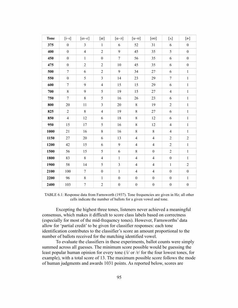
Tone [i~(] [e(~#] [æ] [!~"] [u~)] [o)] [+] [,]

375 0 3 1 6 52 31 6 0

400 0 4 2 9 45 35 5 0

450 0 1 0 7 56 35 6 0

475 0 2 2 10 45 35 6 0

500 7 6 2 9 34 27 6 1

550 0 5 3 14 23 29 7 1

600 7 9 4 15 15 29 6 1

700 8 9 5 19 15 27 4 1

750 7 8 5 16 26 23 6 1

800 20 11 3 20 8 19 2 1

825 2 8 4 19 8 27 6 1

850 4 12 6 18 8 12 6 1

950 15 17 5 16 8 12 4 1

1000 21 16 8 16 8 8 4 1

1150 27 20 6 13 4 4 2 2

1200 42 15 6 9 4 4 2 1

1500 56 15 5 6 8 0 2 1

1800 83 8 4 1 4 4 0 1

1900 58 14 5 3 4 4 1 2

2100 100 7 0 1 4 4 0 0

2200 96 8 1 0 0 0 0 1

2400 103 7 2 0 0 0 0 0

TABLE 6.1: Response data from Farnsworth (1937). Tone frequencies are given in Hz; all other cells indicate the number of ballots for a given vowel and tone.

Excepting the highest three tones, listeners never achieved a meaningful consensus, which makes it difficult to score class labels based on correctness (especially for most of the mid-frequency tones). However, Farnsworths’ data allow for ‘partial credit’ to be given for classifier responses: each tone identification contributes to the classifier’s score an amount proportional to the number of ballots received for the matching identified vowel.

To evaluate the classifiers in these experiments, ballot counts were simply summed across all guesses. The minimum score possible would be guessing the least popular human opinion for every tone (/i/ or /r/ for the four lowest tones, for example), with a total score of 13. The maximum possible score follows the mode of human judgments and awards 1031 points. As reported below, scores are

95

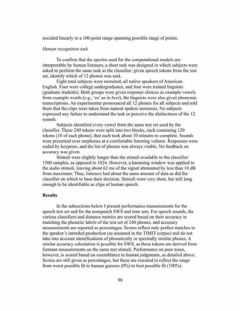
rescaled linearly to a 100-point range spanning possible range of points.

Human recognition task

To confirm that the spectra used for the computational models are interpretable by human listeners, a short task was designed in which subjects were asked to perform the same task as the classifier: given speech tokens from the test set, identify which of 12 phones was said.

Eight total subjects were recruited, all native speakers of American English. Four were college undergraduates, and four were trained linguists (graduate students). Both groups were given response choices as example vowels from example words (e.g., ‘ee’ as in beet); the linguists were also given phonemic transcriptions. An experimenter pronounced all 12 phones for all subjects and told them that the clips were taken from natural spoken sentences. No subjects expressed any failure to understand the task or perceive the distinctness of the 12 sounds.

Subjects identified every vowel from the same test set used by the classifier. These 240 tokens were split into two blocks, each containing 120 tokens (10 of each phone), that each took about 10 minutes to complete. Sounds were presented over earphones at a comfortable listening volume. Responses were coded by keypress, and the list of phones was always visible. No feedback on accuracy was given.

Stimuli were slightly longer than the stimuli available to the classifier: 1500 samples, as opposed to 1024. However, a hamming window was applied to the audio stimuli, leaving about 62 ms of the signal attenuated by less than 10 dB from maximum. Thus, listeners had about the same amount of data as did the classifier on which to base their decision. Stimuli were very short, but still long enough to be identifiable as clips of human speech.

Results

In the subsections below I present performance measurements for the speech test set and for the nonspeech SWS and tone sets. For speech sounds, the various classifiers and distance metrics are scored based on their accuracy in matching the phonetic labels of the test set of 240 phones, and accuracy measurements are reported as percentages. Scores reflect only perfect matches to the speaker’s intended production (as assumed in the TIMIT corpus) and do not take into account identifications of phonetically or spectrally similar phones. A similar accuracy calculation is possible for SWS, as these tokens are derived from formant measurements on the same test stimuli. Performance on pure tones, however, is scored based on resemblance to human judgments, as detailed above. Scores are still given as percentages, but these are rescaled to reflect the range from worst possible fit to human guesses (0%) to best possible fit (100%).

96

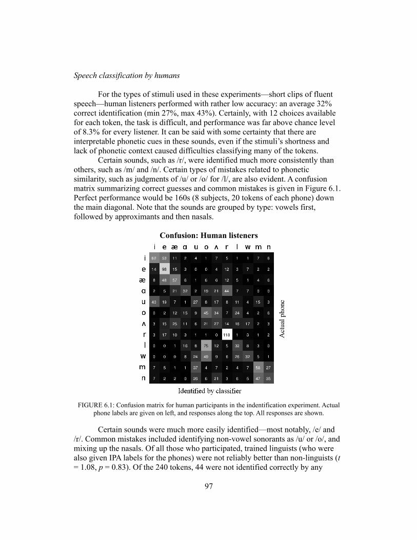
Speech classification by humans

For the types of stimuli used in these experiments—short clips of fluent speech—human listeners performed with rather low accuracy: an average 32% correct identification (min 27%, max 43%). Certainly, with 12 choices available for each token, the task is difficult, and performance was far above chance level of 8.3% for every listener. It can be said with some certainty that there are interpretable phonetic cues in these sounds, even if the stimuli’s shortness and lack of phonetic context caused difficulties classifying many of the tokens.

Certain sounds, such as /r/, were identified much more consistently than others, such as /m/ and /n/. Certain types of mistakes related to phonetic similarity, such as judgments of /u/ or /o/ for /l/, are also evident. A confusion matrix summarizing correct guesses and common mistakes is given in Figure 6.1. Perfect performance would be 160s (8 subjects, 20 tokens of each phone) down the main diagonal. Note that the sounds are grouped by type: vowels first, followed by approximants and then nasals.

Confusion: Human listeners

FIGURE 6.1: Confusion matrix for human participants in the indentification experiment. Actual phone labels are given on left, and responses along the top. All responses are shown.

Certain sounds were much more easily identified—most notably, /e/ and /r/. Common mistakes included identifying non-vowel sonorants as /u/ or /o/, and mixing up the nasals. Of all those who participated, trained linguists (who were also given IPA labels for the phones) were not reliably better than non-linguists (t = 1.08, p = 0.83). Of the 240 tokens, 44 were not identified correctly by any

97

listeners, possibly indicating that these had heavy coarticulation with neighboring segments or were mislabeled in the corpus.

Speech classification by machines

Machine classifiers showed a wide range of accuracy on speech stimuli, although all were higher than chance and generally performed better than human listeners. Accuracy is given in Table 6.2 for statistical and minimum distance classifiers. Tests performed with logged versions of template features are also reported; logging the values de-emphasizes the peaks slightly and accentuates other aspects of spectral shape.

Statistical classifier Score D Distance classifier Score DFormants (Freq only) 55.4% 4 Spectral distance 49.6% 200

F1+F2 40.0% 2 Log spec distance 50.4% 200Formants (F+A) 60.0% 8 EP distance 48.3% 311

Critical bins 52.5% 16 Log EP distance 54.1% 311Log critical bins 67.9% 16

MFCCs 73.3% 10

TABLE 6.2: Accuracy of all computational classifiers on speech, with dimensionality (D) of these classifiers for reference. Formant representations are lightly shaded, and whole-spectrum template

representations more darkly shaded.

Statistical classifiers, if given sufficiently detailed features, are generally better than distance classifiers. (A direct comparison on the same features bears this out as well: implementing the distance criterion for critical bins gives 47.9% accuracy, versus the statistical classifier’s reported 52.5%.) Including amplitudes in the formant model allows a modest boost in performance, as does logging the values of critical bin features. It does appear that the spectral shape representation has a slight edge over the formant representation.

MFCCs, considered here for comparison rather than as a credible model of human perception, outscore all other features. This result might be expected given that the procedure of generating these features has been developed towards a goal of discriminating speech sounds. Confusion matrices for the best performing classifiers (formants with amplitudes, logged critical bins, logged EP distance, and MFCCs) are given in Figure 6.2. As these classifiers are more accurate than human listeners, responses better follow the diagonal. The critical bins and EP distance do show some of the same misidentifications of /l/ and /w/ as /o/ and of the nasals as /u/ that human listeners made.

98

Confusion: Formants Confusion: Logged critical bins

Confusion: Logged EP distance Confusion: MFCCs

FIGURE 6.2: Confusion matrices for four speech-trained and speech-tested classifiers.

Classification of SWS tokens

All of the above classifiers except those that rely on formants were also tested on SWS. Results are given in Table 6.3 (results on speech tests also reprinted for comparison).

99

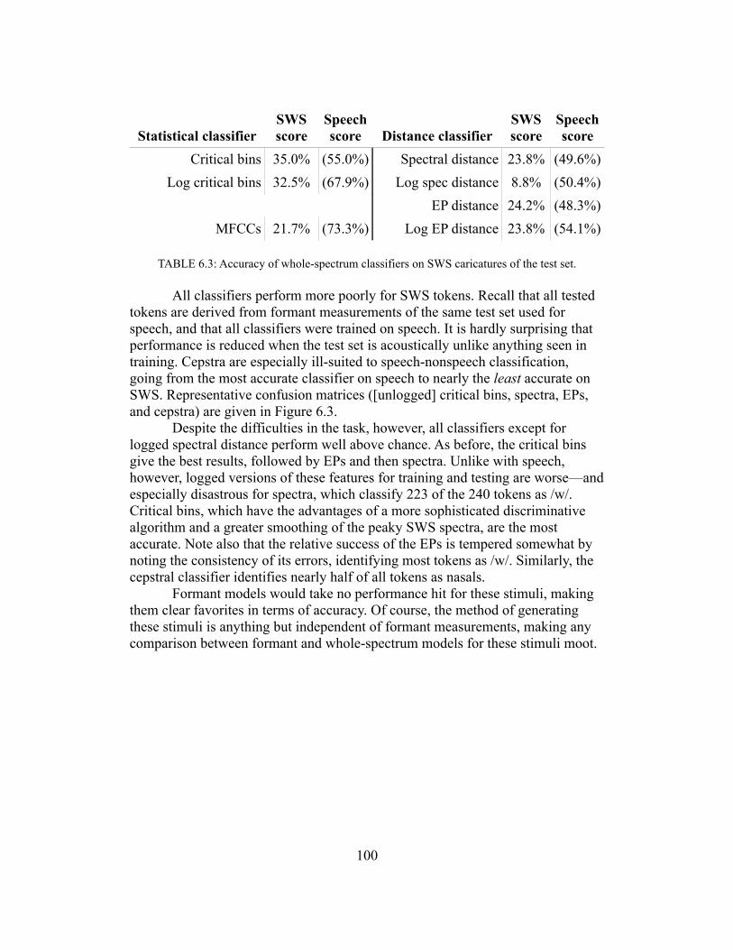
Statistical classifierSWS score

Speech score Distance classifier

SWS score

Speech score

Critical bins 35.0% (55.0%) Spectral distance 23.8% (49.6%)Log critical bins 32.5% (67.9%) Log spec distance 8.8% (50.4%)

EP distance 24.2% (48.3%)MFCCs 21.7% (73.3%) Log EP distance 23.8% (54.1%)

TABLE 6.3: Accuracy of whole-spectrum classifiers on SWS caricatures of the test set.

All classifiers perform more poorly for SWS tokens. Recall that all tested tokens are derived from formant measurements of the same test set used for speech, and that all classifiers were trained on speech. It is hardly surprising that performance is reduced when the test set is acoustically unlike anything seen in training. Cepstra are especially ill-suited to speech-nonspeech classification, going from the most accurate classifier on speech to nearly the least accurate on SWS. Representative confusion matrices ([unlogged] critical bins, spectra, EPs, and cepstra) are given in Figure 6.3.

Despite the difficulties in the task, however, all classifiers except for logged spectral distance perform well above chance. As before, the critical bins give the best results, followed by EPs and then spectra. Unlike with speech, however, logged versions of these features for training and testing are worse—and especially disastrous for spectra, which classify 223 of the 240 tokens as /w/. Critical bins, which have the advantages of a more sophisticated discriminative algorithm and a greater smoothing of the peaky SWS spectra, are the most accurate. Note also that the relative success of the EPs is tempered somewhat by noting the consistency of its errors, identifying most tokens as /w/. Similarly, the cepstral classifier identifies nearly half of all tokens as nasals.

Formant models would take no performance hit for these stimuli, making them clear favorites in terms of accuracy. Of course, the method of generating these stimuli is anything but independent of formant measurements, making any comparison between formant and whole-spectrum models for these stimuli moot.

100

SWS Confusion: Critical bins SWS Confusion: Spectra

SWS Confusion: EPs SWS Confusion: MFCCs

FIGURE 6.3: Confusion matrices for four speech-trained and SWS-tested classifiers.

Classification of tones

Models are scored for tones based on overlap with human judgments. These are divided into three broad ranges: low tones (375 to 750 Hz), which are overwhelmingly identified as back rounded vowels; high tones (1500 Hz and up), which are overwhelmingly identified as a high front vowel; and mid tones between them. (Recall that Table 6.1 pools together certain phones based on overlap with phonetic categories known to the spectral classifiers.)

101

Scores are given in Table 6.4 based on accuracy of all tone frequencies and broken down further for each of the three ranges. Recall the scoring criterion used for this experiment: scores are first calculated by summing the total number of ballots (by human listeners) that agree with the classifier’s judgments across all 22 tones, then linearly rescaled to a 100-point range, 100 corresponding to modal judgments across all tones and 0 corresponding to the least possible agreement with human judgments. Scores in each column of Table 6.4 are rescaled to the maximum and minimum scores of the relevant range for that column, so scores of 100 for every range are possible.

Classifier features Low Mid High Entire rangeAll formants at tone frequency

0.3 8.8 2.0 2.9

Formants,only F2 at tone

77.6 58.6 7.7 39.6

Formants, F2 at tone, amplitudes

87.0 36.7 100 82.7

Critical bins 78.6 35.3 42.0 51.7Log crit bins 80.5 29.3 89.9 74.3Spectral dist 86.0 40.9 44.0 56.1

Log spectral dist 77.6 65.1 23.2 48.5EP dist 77.6 61.4 1.8 37.3

Log EP dist 71.8 63.3 89.9 78.8MFCCs 33.4 58.6 0.8 22.9

TABLE 6.4: Scores for classifiers’ consistency with human judgments of tones. Each condition (column) presents scores on a 100-point scale, with 0 being least consistent and 100 most

consistent with human tone identification.

High overall scores do not necessarily reflect well-tuned classifiers. A dummy classifier that categorizes all tokens as /i/, for example, will receive a relatively high score of 63.2 over the entire range given that so many of the higher tones are identified overwhelmingly as /i/. Therefore, a classifier should have good standing in all three frequency ranges to be considered successful. A table showing how every classifier categorized every tone is given in the appendix.

The formant model that sets all formants to the only frequency present (as some formant tracking algorithms would determine) is aggressively unfit for this task. It classifies all tones as either /r/ or /!/ and woefully underperforms in every frequency range. The more tailored approach of considering the tone to be F2 and

102

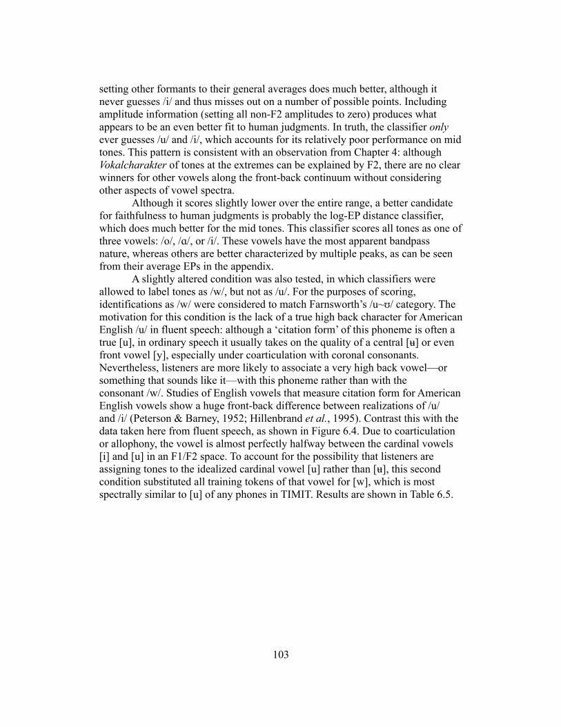
setting other formants to their general averages does much better, although it never guesses /i/ and thus misses out on a number of possible points. Including amplitude information (setting all non-F2 amplitudes to zero) produces what appears to be an even better fit to human judgments. In truth, the classifier only ever guesses /u/ and /i/, which accounts for its relatively poor performance on mid tones. This pattern is consistent with an observation from Chapter 4: although Vokalcharakter of tones at the extremes can be explained by F2, there are no clear winners for other vowels along the front-back continuum without considering other aspects of vowel spectra.

Although it scores slightly lower over the entire range, a better candidate for faithfulness to human judgments is probably the log-EP distance classifier, which does much better for the mid tones. This classifier scores all tones as one of three vowels: /o/, /!/, or /i/. These vowels have the most apparent bandpass nature, whereas others are better characterized by multiple peaks, as can be seen from their average EPs in the appendix.

A slightly altered condition was also tested, in which classifiers were allowed to label tones as /w/, but not as /u/. For the purposes of scoring, identifications as /w/ were considered to match Farnsworth’s /u~)/ category. The motivation for this condition is the lack of a true high back character for American English /u/ in fluent speech: although a ‘citation form’ of this phoneme is often a true [u], in ordinary speech it usually takes on the quality of a central [&] or even front vowel [y], especially under coarticulation with coronal consonants. Nevertheless, listeners are more likely to associate a very high back vowel—or something that sounds like it—with this phoneme rather than with the consonant /w/. Studies of English vowels that measure citation form for American English vowels show a huge front-back difference between realizations of /u/ and /i/ (Peterson & Barney, 1952; Hillenbrand et al., 1995). Contrast this with the data taken here from fluent speech, as shown in Figure 6.4. Due to coarticulation or allophony, the vowel is almost perfectly halfway between the cardinal vowels [i] and [u] in an F1/F2 space. To account for the possibility that listeners are assigning tones to the idealized cardinal vowel [u] rather than [&], this second condition substituted all training tokens of that vowel for [w], which is most spectrally similar to [u] of any phones in TIMIT. Results are shown in Table 6.5.

103

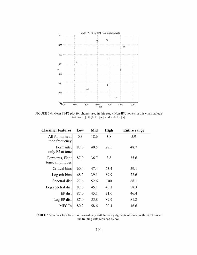
FIGURE 6.4: Mean F1/F2 plot for phones used in this study. Non-IPA vowels in this chart include <a> for [!], <@> for [æ], and <h> for [+].

Classifier features Low Mid High Entire rangeAll formants at tone frequency

0.3 18.6 3.8 5.9

Formants,only F2 at tone

87.0 40.5 28.5 48.7

Formants, F2 at tone, amplitudes

87.0 36.7 3.8 35.6

Critical bins 60.4 47.4 63.4 59.1Log crit bins 68.2 39.1 89.9 72.6Spectral dist 27.6 52.6 100 68.1

Log spectral dist 87.0 45.1 46.1 58.3EP dist 87.0 45.1 21.6 46.4

Log EP dist 87.0 55.8 89.9 81.8MFCCs 80.2 58.6 20.4 46.6

TABLE 6.5: Scores for classifiers’ consistency with human judgments of tones, with /u/ tokens in the training data replaced by /w/.

104

Although the overall pattern of responses in this condition is the same as before, there are some important differences. The logged EPs now identify more sounds as /u/ that before were /o/, resulting in slightly higher overlap with human judgments. Spectral distance also sees a radical shift in performance, with many tokens previously identified as /u/ now falling closest to /i/.

The other major difference is seen in the 8-dimensional formant model, which now identifies everything as /u/. This result probably says more about the fragility of these ad hoc formant and amplitude features as much as it does about any substantive acoustic difference between /w/ and /u/.

Overall, under both conditions, logged distance in the excitation patterns appears to produce the most perceptually plausible mapping of tones to vowels. Other whole-spectrum representations fall short in some ways. The frequency resolution of spectra is probably too fine to provide any meaningful match between tones and the more broadband pole cues of natural speech sounds, and critical bins may over-smooth the spectrum. Under certain conditions, formants also fit the data fairly well, but this requires a few assumptions, foremost of which is that listeners prioritize F2 as the cue to fill when limited spectral information is available. And the F2 representation is fragile when considering the possibility of an idealized back and round [u] as a category prototype; the smoothed spectral representations, EPs and critical bins, are more robust.

Discussion

Accuracy of listeners and of machine classifiers

With the correct classification schemes and feature selection, automated classifiers phonetic classifiers could be made to perform fairly well on these speech data. The gap between well- and ill-suited features is certainly apparent—note the 18-point difference between a simple spectral match versus a critical band representation—but the difference between spectral and formant models is not particularly high, and both are outperformed by cepstral coefficients. In comparison to other studies, the accuracy of these classifiers is rather low—e.g., Hillenbrand and Houde (2003), who apply their model to CVC tokens recorded in isolation—but that discrepancy can almost certainly be accounted for by the nature of the data, which in my experiments are drawn from fluent speech.

Rather than comparing classifier performance to human performance, it was generally assumed that the phonetic labeling of the corpus corresponded to the phones as they were intended to be heard by listeners, and that very few errors in speech or in hand labeling took place. It is not clear that high accuracy necessarily relates to high correlation with human abilities (except in the sense that highly accurate classifiers are picking up only on major inter-category variation). The reduction of information from fluent speech to these spectra is not a normal transformation of an acoustic signal, making any human judgment on

105

these sounds hard to link to ordinary speech perception.Of course, human listeners’ performance in their version of the experiment

could be considered abysmal if compared directly to the machines’. But although the tasks set to the humans and machine classifiers were superficially similar, it is difficult to make any objective comparisons between them because of fundamental differences in how reference categories to which to compare test tokens would be represented. Human listeners were not trained on these exact types of stimuli; rather, it was assumed that their prior experience with American English would give them the necessary spectral exemplars to make sense of the stimuli. Listeners are accustomed to extracting cues to phonetic identity from phonetic context, coarticulation, and other higher-level knowledge. Classifiers were trained directly on similar data to the test set and have no supervised understanding of coarticulation; in a sense, the classifiers have a clear advantage, as the test set comprises stimuli familiar to them but unnatural to listeners. Considering the unnaturalness of the stimuli, total absence of phonetic context information, and attention constraints of the short sound clips, excellent human performance should certainly not be expected. The aim of the human experiment was not to directly compare to classifier performance, but rather to confirm that spectral phonetic cues are still present even following the deletion of phonetically relevant context information.

In these suboptimal conditions, perception in human listeners may not even be especially sensitive to fine spectral details. Spectra alone might only provide sufficient information if they are clearly categorical, or if there is ample time to listen. As was suggested in the discussion in the previous chapter, temporal dynamics might play a role in determining which spectra are most reliable. In the human-listener experiment in this chapter, no spectra could be considered particularly reliable because all were presented very briefly. The listener had no cue alerting them to which frequencies in the spectrum were especially critical.

Interpreting SWS findings

The fact that nonspeech created as a formant-based caricature of normal speech is intelligible is prima facie support for the notion of formants as true perceptual objects. This impression follows directly from the strategy for generating SWS: synthesize three or four FM tones and add them together. To the perceptual system, however, it may be more useful to consider that the concurrent tones generate spectra just as would any other sounds. From this perspective, there is no reason to believe that a generic approach to spectral recognition should not be able to successfully process SWS spectra.

In terms of success, the results in the current chapter were mixed. Some strategies did fairly well at identifying vowels, although certainly not as well as for speech. Some degradation of spectral cues, and thus a drop in performance,

106

was certainly to be expected. The most disastrous drop was with cepstra, which so aptly capture shape cues for speech but cannot apply those to nonspeech. The results suggest that, although many phonetically relevant cues are preserved in generating SWS, those features that are picked up by cepstra and highly effective for discrimination are not preserved. Affected cepstral cues, while discriminatively powerful, appear to be perceptually irrelevant for the purposes of these sounds.

The suitability of a template-matching strategy as a model for human identification of SWS was also tested directly by Hillenbrand et al. (2011). Applying Hillenbrand and Houde’s (2003) narrow-band spectral template model to SWS vowels—trained on speech and tested on SWS, as in my experiments here—they find accuracy equaling human performance after training on SWS vowels, and easily surpassing performance by naïve listeners. They conclude that the results do not rule out a template-based perceptual strategy for SWS.

Of the spectral shape approaches tested here, those with higher degrees of smoothing had higher accuracy. Note, however, that peripheral auditory smoothing is likely not inconsistent with the pooling of energy within critical bands, and certainly not inconsistent with the smoothing in calculating the EP. That is, the spectral smoothing that is inherent to an auditorily plausible model is also helpful in making SWS representations match those of fully spectral speech.

As mentioned earlier, it is unclear how to compare performance of formant and whole-spectrum models on SWS. It might be said, however, that a formants-only account for SWS is somewhat unsatisfying because it predicts that spectral cues are perfectly retained, despite the fact that intelligibility is reduced for SWS. In fact, this account should predict that SWS is even easier to process than speech, as the peaks are more clearly resolvable.

Of course, all of the above conclusions rest on a fundamental assumption made in the setup of this experiment: that the intended phones by speakers would match the actual perceived phones by listeners. True labels of the test set were kept and not re-validated for the SWS tokens constructed from formant measurements. A more rigorous approach might be to obtain human judgments for each of these tokens; however, the nature of SWS makes these judgments difficult to obtain reliably because listeners do not usually hear these sounds as speech unless they are in longer utterances. The fact that SWS sentences are intelligible suggests that their spectra are not dramatically divergent from natural vowel spectra. The 2011 study by Hillenbrand and colleagues mentioned above found human identification of isolated SWS vowels far above chance, and yet still falling well short of accuracy on speech. There may be inconsistencies between the phonetics ultimately derived from SWS sentences and the spectra that the stimuli most closely resemble perceptually, which are squashed ultimately by lexically driven top-down effects. Furthermore, and perhaps more seriously, SWS may not rely heavily on spectral perception, but rather on detection of rapid modulations signaling consonants and other transitions. Either way, it is probably

107

not incumbent upon spectral perception to fully explain the intelligibility of sentences in SWS; other abilities will have to be invoked.

Issues in modeling Vokalcharakter

Certain of the spectral classifiers were impressively reflective of human vowel judgments of pure tones. Although uncontroversial category labels will never be available for such nonspeech stimuli as pure tones, the huge number of responses solicited by Farnsworth (1937) provides a rather straightforward manner of comparing classifier outputs with the ‘best’ human judgments. Whole-spectrum representations based on the excitation pattern provided the best match, and they even preferentially captured those phones ([w], [o], [!], [i]) that are best defined spectrally by a single frequency peak.

Substituting the spectral quality of /w/ for the usually fronted American English /u/ did not have a dramatic impact on the accuracy of an EP classifier, but I do think that the nature of the /u/ category is important to consider. Without a clear [u] cardinal vowel, English lacks a vowel with a strong low-pass characteristic. Certain consonants, such as [w] and [m], do have this nature (Fant [1973] saw very low tones identified sometimes as [m] rather than [u]), but may also have phonological properties that make them less suitable labels for tones. Moreover, the /u/ considered here differs in its acoustic realization from measurements of citation vowels of American English. I contend that the very low tones labeled as /u/ are, in the minds of listeners, closer to [u] than to [&]. Working from this assumption saw the EP classifier identifying vowels as /u/, /!/, and /i/ rather than /o/, /!/, and /i/, providing a slightly better fit to the data. Nevertheless, while this modification did raise the score for the EP classifier, a strong performance in the initial condition is evidence enough to demonstrate the power of a spectral shape classifier relative to a formant-based classifier.

Although it is the most comprehensive study on the matter, there are reasons why Farnsworth’s paper might not be an ideal authoritative source for tonal Vokalcharakter for English-speaking listeners. Although the methods are mostly clear, the example words presented to listeners are inconsistent in vowel nasality, which might affect the spectrum in a number of ways—for example, the de-emphasis of lower pole cues through the introduction of nasal anti-formants. There are also a few anomalies in the data may be cause for concern; in particular, the vowels [i] and [(] are surprisingly common responses for tones even as low as 800 Hz, which is well below what other studies of the phenomenon have shown: Kuhl et al. (1991) grouped tones as high as 1500 Hz in their low set, which saw more [!] identification than [i], and my own experiments in Chapter 4 showed that FM tones falling to 1081 Hz were not enthusiastically labeled as the glide [j], which is acoustically similar to [i]. Even the study’s age is a potential concern: with the half century between Farnsworth’s measurements and the recording of the TIMIT corpus, there may have been some modest vowel shift creating

108

inconsistencies between the 1980s vowels in the training set and the tone judgments based on 1930s vowels. Farnsworth’s results are in general qualitative agreement with other studies on the matter, and his subject pool is large; nevertheless, one wonders if the same study conducted with better speech controls and modern subjects and equipment would achieve slightly different results.

Pole-based versus whole spectrum-based representations

The major theoretical question posed at the beginning of this chapter contrasted models of spectral perception that rely on formants and those that rely on templatic or whole-spectrum matching strategies. In the previous chapter, I expressed a certain skepticism for formants for a number of reasons, mostly having to do with their implausibility rather than their inadequacy.

This chapter addressed the adequacy question by testing formants for nonspeech tones. (Elsewhere in the chapter, formants were found to be adequate descriptors for speech spectra, although not quite as good as shape models, and could not be fairly evaluated for SWS.) The results generally show a preference for spectral shape over formants, for at least two reasons. First, the question of how to represent formants for the tone stimuli was not even a straightforward one. An approach that simulated a formant tracking algorithm by setting all formants to the single spectral prominence yielded a fabulously poor match to human judgments. (It is conceivable that other statistical classification algorithms than the one used in these experiments would do better, although credit then would lie with the classifier and not the features used.) A much better fit was found using the prior observation that F2 seemed to be the formant with the best Vokalcharakter match and assuming that a listener would hear a pure tone as an F2. But even in this case, which is already poorly motivated as it is, it is unclear whether including formant amplitude as a predictor should improve the classifier. In one condition, it did (by identifying all tokens as /u/ or /i/), but not when considering [w] tokens as exemplars of the /u/ class (when including amplitudes caused all tokens to be identified as /u/). Formant classifiers trained on speech only perform well for tones when appealing to ad hoc measures, and even then it was unclear how to account for the hypothetical amplitude difference between a tone’s F2 and its other formants.

The second objection comes from the simple fact that template-based approaches outperformed the formant classifier. For both conditions tested, the only scheme that consistently performed well over all ranges was the simple distance classifier over (logged) excitation patterns. Even the critical bin representations, which were so effective for speech, proved to be too much of a reduction in data to compete with the EPs. This model was exceedingly simple in its assumptions—cochlear filtering, plus a simple distance function—but solidly outperforms other models for this task. The success of this model suggests the power of even rather unsophisticated, naïve template models. Certainly more

109

tuning would have to be done to perfectly recreate a human strategy (and note that even human listeners are not in total agreement with tone classification), but the immediate success of a template model—versus the tortured and measured success of a formant model—lends support to a whole-spectrum theory of spectral perception.

Logging of templates

The immediately preceding discussion of whole-spectrum representations ignores a very visible wrinkle in the experiment design, which is that spectral shape classifiers were tested with raw feature values as well as with logarithm-transformed features. There is not an obvious principled reason for choosing one version of the features over the other. The predominant practical effect of logging a template representation is to compress the amplitude range somewhat. In doing so, error/distance functions become less sensitive to variation in peaks while mostly retaining sensitivity to moderate degrees of amplitude. Classifiers become more forgiving of differences in peak height. In physiological terms, untransformed version of EPs and critical bins reflect the degrees of activation at some stage of the peripheral auditory system; logging might be considered a coarse simulation of compression occurring at or beyond the auditory nerve. (The successes of logged features in the experiments here suggest that some compression before calculation of distance is probably consistent with auditory processing, although it is certainly more sophisticated than a logarithm.)

The application of this logging compression is beneficial for all spectral classifiers for speech. For nonspeech, the picture becomes cloudier. Logging is always unhelpful for SWS, breaking the spectral distance classifier entirely, although the effects on EPs and critical bins are minimal. For tones, logging is helpful for EPs and critical bins but not for spectra. A clear conclusion is that logging is disastrous for sparse spectra such as those of SWS or pure tones. These spectra will have many values close to zero, which can greatly distort the logarithm, causing anti-compression as it approaches negative infinity. EPs are more resistant to this distortion, as the broadness of the cochlear filters result in excitation across the spectrum for input. The unsuitability of spectra for logging appears to have to do more with the nature of the logarithm than with the fact that compression is applied.

Why, then, is logging so beneficial for EPs in the tone case but not for SWS? The answer here may lie in the fundamental differences between the correct responses. The best identifications for tones are vowels that typically have a narrowband characteristic, and logged EPs captured this quite well by enhancing the difference between areas of low and moderate energy. The SWS vowels had no such shared acoustic characteristic; indeed, all phones were subjected to the SWS treatment, whether or not three peaks is a reasonable way to represent them. In these cases, the reduced accuracy of matching in the spectral troughs would

110

have penalized phones that are characterized by sections of energy that are not captured by the three dominant peaks.

Zero cues

The nature of these narrowband vowels raises an issue that was first mentioned in Chapter 4: an impressionistic survey of tonal Vokalcharakter for English speakers and perception of filtered vowels suggests that spectral gaps, or at least sharp falloffs from prominences, constitute important cues in their own right. The absence of energy within a band may be just as critical to a vowel’s identity as the presence of energy in others. Seen in this light, common Vokalcharakter correspondences made sense—[i] having a major gap below F2, [u] a major gap above F2, and [!] major gaps on either side of the F1/F2 band. Poles are certainly salient cues to vowel quality, and other cues in the spectrum important to voice quality or consonant identity, but these zeros too are powerful enough to restrict the hypothesis space for identifying tokens.

The experiments in this chapter did not directly address these positive zero cues or make any claims about how they might be represented by the auditory system. However, it is worth considering how those zeros would be captured by formant and spectral shape models. When measuring spectral distance, zeros are no different functionally from peaks: a point of significant mismatch between two spectra could either be one’s failing to contain a pole feature or the other’s failing to contain a zero feature. These distance measures are especially sensitive to the zeros of pure tones, as penalties in distance will be incurred across the spectrum. Because spectra and EPs were normalized for this experiment, very peaky spectral prototypes will have non-peaks of very low energy, and thus make inherently better matches for tones (assuming a peak matches the tone in frequency); spectra with wide, shallow peaks, on the other hand, will be heavily penalized. The high correlation observed in these experiments between spectral template modeling and human judgments suggests that human listeners also penalize prototype vowel spectra that contain wide bands of energy where the tone has none.

Although formant frequencies do not explicitly model anything happening between peaks, some conjectures can be made about how zeros might be represented. In most cases, a large separation between formant frequencies would suggest the presence of a zero between them (and similarly, a very high F1 would suggest a low-frequency zero). The problem is that these zeros cannot be guaranteed; sharper peaks will fall off to more detectable zeros, and sharpness cannot be determined from frequency and amplitude alone. Some information correlating with zero cues will remain in formant representations, although it will not be as reliable as that remaining in spectral representations.

111

Cepstra and the perception of spectral shape

As discussed in the previous chapter, mel-frequency cepstra, though warped to a psychoacoustic scale, are not a realistic reflection of what is happening in the auditory system. They are fantastically useful for encoding spectral shape for speech, which panned out in this experiment as well: truncating the coefficients to just ten produced a better classifier than any other method. For nonspeech, however, cepstra fell well short of most other models. As mentioned above in the discussion of SWS, cepstra appear to be picking up on cues that have ample discriminating power for speech but, as evidenced by their unsuitability for speech-nonspeech stimuli, may be perceptually irrelevant. The unsuitability of cepstra for nonspeech runs parallel to the deleterious effects that noise have on cepstra for speech. One could even consider the nonspeech sounds to be speech passed through some nonlinear noisy channel, which human listeners are able to correct for. Part of the fragility of cepstra lies in their non-locality: human perception of energy within a critical band is minimally affected by out-of-band energy, whereas cepstra are sensitive to disruptions across the frequency range (Allen, 1994). A particularly relevant attempt to describe shape detection in the central auditory system comes from Wang and Shamma (1995b), who present a mathematical model that shares spiritual and functional similarities to a localized cepstral analysis.

True perception probably does rely on parameters related to overall shape, possibly some type of spectral shape primitives, which the template approach might accidentally capture but cannot explicitly model. Cepstra capture aspects of spectral shape in a Fourier-analytic sense by tracking slower or more rapid oscillations in spectral envelope. Although more explicitly addressing spectral shape than the template models, cepstra are still largely unsupervised and untuned in terms of the aspects of shape that they capture. An effective strategy for modeling human perception would be one that recognizes key shape variables at a central-modeling level while still retaining the advantages of template matching at a peripheral-modeling level.

Conclusion

The experiments in this chapter tested the efficacy of certain spectral or formant features for the classification of speech and nonspeech sounds, using both simple distance criteria as well as machine learning methods. Although the approach is not altogether novel, some of the data considered are. I was concerned primarily with testing an old debate, on the efficacy and appropriateness of formant-based versus whole spectrum-based classifiers, using narrow-band stimuli like tones that have been shown in this dissertation and elsewhere to have perceptual correlates in speech sounds.

The intuition at the heart of the experiment design is that a machine

112

‘listener’ trained only on speech sounds should be able to make speech judgments on nonspeech tokens. If these judgments are in line with responses by human listeners, then that constitutes some evidence that the features selected by the classifier are reflective of some real features in speech perception. Attempts to boil down features to low-dimensional representations, via either formants or cepstra, are successful for normal speech sounds but not for nonspeech, indicating that perhaps the motivations for using such representations are more based on their happenstance suitability for describing speech sounds and less on actual auditory processing.

Experiments here provide support for a whole-spectrum approach with a built-in consideration of peripheral audition. Certain questions as to how to tune the model remain: What is the ideal bandwidth of integration? What is the most accurate strategy for applying compression? How can key variables about shape be captured in a way that preserves the advantages of the template model? These will have to be addressed for a thorough modeling of phonetic spectral perception. And, as discussed in the previous chapter, the adequacy of even perfect spectral modeling should be considered in the grander picture of spectrotemporal processing.

113

ConclusionThe work in this dissertation constitutes a number of novel contributions

to the speech perception literature. I summarized in Chapter 2 a line of research in speech-nonspeech perception that did not have a cohesive identity or unified approach (or a name, for that matter). The experiments in Part II added further to this body of work. Those in Chapter 3 demonstrated the phonetic reality of speech-nonspeech in a way that had not been previously shown, and Chapter 4 contained further evidence that tonal Vokalcharakter, an incredibly subtle and understudied effect, operates along the temporal dimension similarly to speech. Finally, in Part II I approached a line of research in modeling human perceptual processes and applied nonspeech data that had not before been considered for such models.

Thematically, these contributions have all been tied together by a nonspeech thread, but each chapter has considered its own perspectives and its own speculative leads. There are two minor theoretical points, and one major one, that I would want any reader to take away from this dissertation. I start with the minor points: the first is somewhat more philosophical or cognitive, and associated primarily with Chapters 2-4, while the second is more implementational and associated more with Chapters 4-6.

The first point to call attention to is that the perception of speech is a necessarily flexible process, acting upon any auditory stimulus, whether consciously addressed as speech or not. It is, I think, another facet of more general perceptual mechanisms that act to understand the world by any means available. Perception, as an interface between reality and experience, is part psychophysics, part metaphor. Speech is a tremendously important stimulus for virtually every human being, for obvious reasons. It should perhaps come as no surprise that we hear speech around every corner, the same way we see a face in the most cartoonish or even accidental representations. Understanding how the expectation for speech can guide hearing has implications for the study of language, too—everything from the study of onomatopoeia and sound symbolism to grander questions about the origins of language.

The second minor point concerns a more practical consequence for the study of speech perception. Chapters 5 and 6 addressed what should by now be a more obvious realization for researchers in the field: auditory spectral perception operates on auditory spectra. That is to say, there is very little empirical support anymore for a highly reductionist picture of spectral perception that relies on cues that, though tremendously influential in shaping acoustic theories of speech, are neither auditorily realistic nor descriptively adequate for speech perception more nuanced than identifying vowel quality. Researchers in perception should discard a long-held, convenient, even comforting notion that we need only address the resonances of the vocal tract to understand its perceptual consequence. (Of course, outside of perception, formants are still hugely illustrative from an

114

articulatory and acoustic standpoint.) The nature of phonetic categories needs to be rethought from the ground up. Even research that acknowledges the flaws in formant representations is still driven inexorably by that old intuition—for example, parameters for the synthesis or even the description of speech sounds are expressed in formant measurements. However acoustically descriptive these are, their continued use discourages a hard consideration of how perception actually works. The current state of spectral perception modeling gives us no useful agreement on the nature of spectral shape features; a naïve distance measure between some kind of auditory spectrum is about as sophisticated as it gets.

These two seemingly disjoint conclusions, one about the nature of perception in general and one about the details of spectral perception, come together to support a grander idea that has cropped up again and again through the course of these experiments. Phonetic perception (and not only phonetic perception) operates by a process of inference and decision based on some calculation of the likelihood of natural events. It does not presuppose the speech or nonspeech state of incoming sounds, nor does it perform a qualitatively different acoustic analysis when considering speech—the specialness of speech comes out of inference about language and about articulatory dynamics, which are highly flexible but acoustically natural nonetheless. Elements of both general auditory and gesture-based theories of speech perception are essential: listeners can differentiate phonetically distinct events using general auditory abilities, but an understanding of the acoustic system producing them is what leads to the robust recovery of the talker’s message. Direct realism is an elegant philosophical characterization of the process: when hearing speech and other sounds, listeners perceive sources, not frequencies or transients or noise. Their judgments as to the nature and mechanics of these sources are supported by scene analysis and inference based on multimodal inputs.

Another theoretical controversy addressed earlier concerns two approaches to explaining phonetic categorization: a generative or Bayesian process, in which listeners incorporate prior knowledge of sound generation to perform an analysis by synthesis; or a bottom-up, cue-combinative process, which sorts through auditory cues and finds triggers to categorization. The perspective I espouse here, as an inference-driven process, is perfectly in line with the former. Prior support for inference at play in speech-nonspeech classification comes can be found in the studies with filtered vowels mentioned in Chapters 2 and 4, and especially from cases of restoration of cues in noise. Phonetic identity was severely disrupted by the dramatic filtering of vowels, as doing so introduced apparent zeros into the spectrum, making it ultimately a better templatic fit for vowels that tend to lack energy at the stopped frequencies. With the addition of interfering noise, however, listeners were able to attribute the noise to a separate source and ignore those parts of the spectrum deemed unreliable due to interference. Through what resembles a generative modeling of target and interferer, listeners were able to

115

base their judgments on the most informative cues.The same type of inference can be seen in some of the studies by Kiefte

and Kluender (2005, 2008) cited in Chapter 5. In these experiments, spectral and spectrotemporal features were weighted by listeners not through an inherent advantage for one type of feature over another, but by their compatibility with an analyzed scene. Gross spectral matching through tilt was trusted in the presence of an apparent acoustic resonator, whereas peaks were trusted in the presence of an apparent low- or high-pass filter. When modulations were present, these were considered solid cues to articulation—this too is consistent with scene analysis and inference, as rapid modulations are overwhelmingly more likely to be aspects of a speech source than of an acoustic environment.

My original behavioral experiments in Chapters 3 and 4 build on the support for the inference-based approach. Speech-nonspeech processing was shown to be at work in compensation for coarticulation, with a very important wrinkle: the magnitude of a context effect depended on the plausibility of speech as a source for the context vowel. The effect with nonspeech is weaker than for speech; furthermore, it disappears entirely when lengthening the vowel, whereas the same lengthening enhances the effect for speech vowels. This lengthening increases the amount of information available to the listener, making an unlikely speech source more unlikely, and a likely speech source more likely. The degree of compensation was driven not by auditory contrast or even by a perceived rate of speech so much as it was driven by the likelihood of a speech vowel that could generate an articulatorily predictable acoustic effect on the preceding fricative.

Pure tones were found to be acoustically so unlike speech that it was difficult to show them triggering compensation for coarticulation; as with the long single-formant vowels, listeners deemed them as too improbable as utterances by a human talker. Nevertheless, it is undeniable that it is the tendency for Vokalcharakter, the forced phonetic interpretation of a tone, to follow spectral similarity. (The computational modeling in Chapter 6 confirmed empirically that Vokalcharakter associations across the frequency range could be explained by spectral template matching and the band-pass nature of certain vowels.) The experiments in Chapter 4 assessed the relationship between the Vokalcharakter phenomenon and ordinary speech perception through an audiovisual pairing that eschewed phonetic labeling in favor of a more holistic approach in pairing articulatory knowledge with acoustic outputs. The findings confirmed that listeners’ preferred pairings between articulation and acoustics were driven by maximizing the temporal and spectral similarities between them.

The experiments and literature review undertaken in this dissertation consistently provide support for such an approach; specifying the details will have to be the focus of future work. Analyzing the nature of perception in any modality is a monumental task, and the findings held in these pages are, I can only hope, a small step towards completing it. The value of speech-nonspeech has certainly been made evident, as have the usefulness and flaws of a number of notions with

116

which researchers approach their work on perception. I end this dissertation with the hope that the results and ideas contained herein point the way towards a betterment, however humble, of our sciences of phonetics, psychology, and linguistics.

117

References

Allen, J. B. (1994). How Do Humans Process and Recognize Speech? IEEE Transactions on Speech and Audio Processing 2 (4), 567–573.

Assmann, P. F. (1991). The Perception of Back Vowels: Centre of Gravity Hypothesis. The Quarterly Journal of Experimental Psychology 43A (3), 423–448.

Bashford, J. A., Warren, R. M., & Lenz, P. W. (2005). Enhancing intelligibility of narrowband speech with out-of-band noise: Evidence for lateral suppression at high-normal intensity. The Journal of the Acoustical Society of America 117 (1): 365–369.

Berent, I., Balaban, E., Lennertz, T., & Vaknin-Nusbaum, V. (2010). Phonological Universals Constrain the Processing of Nonspeech Stimuli. J. Exp. Psychol. 139 (3): 418–435.

Best, C. T. (1995). A direct realist perspective on cross-language speech perception. In Strange, W. (Ed.) Speech perception and linguistic experience: Theoretical and methodological issues in cross-language speech research, 167–200. Timonium, MD: York Press.

Best, C. T., Morrongiello, B., & Robson, R. (1981). Perceptual equivalence of acoustic cues in speech and nonspeech perception. Perception & Psychophysics 29 (3), 191–211.

Bladon, R. A. W. (1982). Arguments against formants in the auditory representation of speech. The representation of speech in the peripheral auditory system, 95–102. Elsevier Biomedical Press.

Bladon, R. A. W. (1983). Two-formant models of vowel perception: shortcomings and enhancements. Speech Communication 2, 305–313.

Bladon, R. A. W. (1986). Phonetics for hearers. In G. McGregor (Ed.) Language for Hearers. Oxford: Pergamon.

Bladon, A., & Fant, G. (1978). A two-formant model and the cardinal vowels. Speech Transmission Laboratory Quarterly Progress and Status Report, 19 (1), 1–8.

Bladon, R. A. W., and Lindblom, B. (1981). Modeling the judgment of vowel quality differences. The Journal of the Acoustical Society of America 69 (5), 1414–1422.

Bladon, R. A. W., Henton, C. G., & Pickering, J. B. (1984). Towards an auditory theory of speaker normalization. Language & Communication 4 (1), 59–69.

Broad, D. J., & Clermont, F. (1989). Formant estimation by linear transformation of the LPC cepstrum. The Journal of the Acoustical Society of America 86 (5), 2013–2017.

Brugge, J. F., & Merzenich, M. M. (1973). Responses of neurons in auditory cortex of macaque monkey to monaural and binaural stimulation. Journal of Neurophysiology 36, 1138–58.

118

Carlson, R. P., Granström, B., & Fant, G. (1970). Some studies concerning perception of isolated vowels. Speech Transmission Laboratory Quarterly Progress and Status Report 11 (2-3), 19–35.

Carlyon, R. P., Deeks, J., Norris, D., & Butterfield, S. (2002). The Continuity Illusion and Vowel Identification. Acta Acustica united with Acustica 88, 408–415.

Chi, T., Ru, P., & Shamma, S. A. (1999). Spectro-temporal modulation transfer functions and speech intelligibility. The Journal of the Acoustical Society of America 106 (5), 2719–2732.

Chi, T., Ru, P., & Shamma, S. A. (2005). Multiresolution spectrotemporal analysis of complex sounds. The Journal of the Acoustical Society of America 118 (2), 887–906.

Chiba, T., & Kajiyama, M. (1958). The Vowel: Its Nature and Structure. Phonetic Society of Japan.

Chistovich, L. A., & Lublinskaya, V. V. (1979). The ‘Center of Gravity’ Effect in Vowel Spectra and Critical Distance Between the Formants: Psychoacoustical Study of the Perception of Vowel-Like Stimuli. Hearing Research 1, 185–195.

Cooke, M., Green, P., Josifovski, L., & Vizinho, A. (2001). Robust automatic speech recognition with missing and unreliable acoustic data. Speech Communication 34, 267–285.

Cooper, F. S., Delattre, P. C., Liberman, A. M., Borst, J. M., & Gerstman, L. J. (1952). Some Experiments on the Perception of Synthetic Speech Sounds. The Journal of the Acoustical Society of America 24 (6), 597–606.

Crowder, R. G., & Repp, B. H. (1984). Single formant contrast in vowel identification. Perception & Psychophysics 35 (4), 372–378.

Cunningham, S. (2003). Modelling the recognition of band-pass filtered speech. Doctoral dissertation, University of Sheffield.

Darwin, C. (2009). SWS (Praat script). http://www.lifesci.sussex.ac.uk/home/Chris_Darwin/Praatscripts/SWS

Davis, M. H., & Johnsrude, I. S. (2007). Hearing speech sounds: Top-down influences on the interface between audition and speech perception. Hearing Research 229, 132–147.

Davis, M. H., Johnsrude, I. S., Hervais-Adelman, A., Taylor, K., & McGettigan, C. (2005). Lexical Information Drives Perceptual Learning of Distorted Speech: Evidence From the Comprehension of Noise-Vocoded Sentences. Journal of Experimental Psychology 134 (2), 222–241.

Delattre, P., Liberman, A. M., Cooper, F. S., & Gerstman, L. J. (1952). An experimental study of the acoustic determinants of vowel color: observations on one- and two-formant vowels synthesized from spectrographic patterns. Word 8, 195–210.

Delgutte, B. (1980). Representations of speech-like sounds in the discharge patterns of auditory-nerve fibers. The Journal of the Acoustical Society of

119

America 68 (3), 843–857.DeWitt, I., & Rauschecker, J. P. (2012). Phoneme and word recognition in the

auditory ventral stream. Proceedings of the National Academy of Sciences 109 (8), E505–E514.

Diehl, R. L., Lotto, A. J., & Holt, L. L. (2004). Speech Perception. Annual Review of Psychology 55, 149–79.

Dorman, M. F., Loizou, P. C., & Rainey, D. (1997). Speech intelligibility as a function of the number of channels of stimulation for signal processors using sine-wave and noise-band outputs. The Journal of the Acoustical Society of America 102 (4), 2403–2411.

Eaton, J. W., Bateman, D., and Hauberg, S. (2009). GNU Octave version 3.0.1 manual: a high-level interactive language for numerical computations. CreateSpace Independent Publishing Platform. http://www.gnu.org/software/octave/doc/interpreter/

Eisenberg, L. S., Shannon, R. V., Schaefer Martinez, A., Wygonski, J., & Boothroyd, A. Speech recognition with reduced spectral cues as a function of age. The Journal of the Acoustical Society of America 107 (5), 2704–2710.

Elliott, T. M., & Theunissen, F. E. (2009). The Modulation Transfer Function for Speech Intelligibility. PLoS Computational Biology 5 (3), e1000302.

Elliott, T. M., Hamilton, L. S., & Theunissen, F. E. (2013). Acoustic structure of the five perceptual dimensions of timbre in orchestral instrument tones. The Journal of the Acoustical Society of America 133 (1), 389–404.

Ellis, D. P. W. (2005). PLP and RASTA (and MFCC, and inversion) in Matlab. Available at http://www.ee.columbia.edu/~dpwe/resources/matlab/rastamat/.

Elman, J., & McClelland, J. (1988). Cognitive Penetration of the Mechanisms of Perception: Compensation for Coarticulation of Lexically Restored Phonemes. Journal of Memory and Language 27, 143–165.

Engelhardt, V., & Gehrcke, E. (1930). Vokalstudien: eine akustisch-psychologische Experimentaluntersuchung über Vokale, Worte und Sätze. JA Barth.

Fant, G. (1971). Acoustic theory of speech production: with calculations based on X-ray studies of Russian articulations (Vol. 2). Walter de Gruyter.

Fant, G. (1973). Speech sounds and features. Cambridge: MIT Press.Fant, G., & Risberg, A. (1963). Auditory matching of vowels with two formant

synthetic sounds. Speech Transmission Laboratory Quarterly Progress and Status Report 4 (4), 7–11.

Farnsworth, P. R. (1937). An Approach to the Study of Vocal Resonance. The Journal of the Acoustical Society of America 9, 152–155.

Fastl, H., & Zwicker, E. (2007). Psychoacoustics: Facts and Models (3rd edition). Berlin: Springer.

Finley, G. P. (2012). Partial effects of perceptual compensation need not be

120

auditorily driven. UC Berkeley Phonology Lab Annual Report, 169–188.Fisher, W. M., Doddington, G. R., & Goudie-Marshall, K. M. (1986). The

DARPA speech recognition research database: specifications and status. Proc. DARPA Workshop on speech recognition, 93–99.

Fowler, C. A. (1986). An event approach to a theory of speech perception from a direct-realist perspective. Journal of Phonetics 14, 3–28.

Fowler, C. A. (1990). Sound-producing sources as objects of perception: Rate normalization and nonspeech perception. The Journal of the Acoustical Society of America 88 (3), 1236–1249.

Fowler, C. A., Best, C. T., & McRoberts, G. W. (1990). Young infants’ perception of liquid coarticulatory influences on following stop consonants. Perception & Psychophysics 48 (6), 559–570.

Fowler, C. A., Brown, J. M., & Mann, V. A. (2000). Contrast effects do not underlie effects of preceding liquids on stop-consonant identification by humans. Journal of Experimental Psychology: Human Perception and Performance 26, 877–88.

Fowler, C. A., & Magnuson, J. S. (2012). Speech Perception. In M. Spivey, K. McRae, & M. Joanisse (Eds.), The Cambridge Handbook of Psycholinguistics. Cambridge University Press.

Fowler, C. A., & Rosenblum, L. D. (1990). Duplex Perception: A Comparison of Monosyllables and Slamming Doors. Journal of Experimental Psychology: Human Perception and Performance 16 (4), 742–754.

Ganong III, W. F. (1980). Phonetic Categorization in Auditory Word Perception. Journal of Experimental Psychology: Human Perception and Performance 6 (1), 110–125.

Gibson, J. J. (1966). The problem of temporal order in stimulation and perception. Journal of Psychology 62, 141–129. Reprinted in E. Reed & R. Jones (Eds.), Reasons for realism. Hillsdale, NJ: LEA, 1982.

Gibson, J. J. (1979). The ecological approach to visual perception. Boston: Houghton-Mifflin.

Gold, B., Morgan, N., & Ellis, D. (2011). Speech and Audio Signal Processing. Hoboken, NJ: John Wiley & Sons, Inc.

Helmholtz, H. L. F. (1954). On the sensations of tone as a physiological basis for the theory of music (A. J. Ellis, Trans.; original German work published 1877). New York: Dover.

Hermansky, H. (1990). Perceptual linear predictive (PLP) analysis of speech. The Journal of the Acoustical Society of America 87 (4), 1738–1752.

Hill, F. J., McRae, L. P., & McClellan, R. P. (1968). Speech Recognition as a Function of Channel Capacity in a Discrete Set of Channels. The Journal of the Acoustical Society of America 44 (1), 13–18.

Hillenbrand, J. M., & Houde, R. A. (2003). A narrow band pattern-matching model of vowel perception. The Journal of the Acoustical Society of America 113 (2), 1044–1055.

121

Hillenbrand, J. M., Clark, M. J., & Baer, C. A. (2011). Perception of sinewave vowels. The Journal of the Acoustical Society of America 129 (6), 3991–4000.

Holt, L. L. (2005). Temporally non-adjacent non-linguistic sounds affect speech categorization. Psychological Science 16, 305–312.

Holt, L. L. (2006). The mean matters: Effects of statistically defined nonspeech spectral distributions on speech categorization. The Journal of the Acoustical Society of America, 120 (5), 2801–2817.

Holt, L. L., & Lotto, A. J. (2002). Behavioral examination of the neural mechanisms of speech context effects. Hearing Research 167, 156–169.

Holt, L. L., Lotto, A. J., & Kluender, K. R. (2000). Neighboring spectral content influences vowel identification. The Journal of the Acoustical Society of America, 108 (2), 710–722.

Hufnagle, D. G., Holt, L. L., & Thiessen, E. D. (2013). Spectral information in nonspeech contexts influences children’s categorization of ambiguous speech sounds. Journal of Experimental Child Psychology 116 (3), 728–737.

International Organization for Standardization. (2003). ISO 226:2003 Acoustics—Normal equal loudness-level contours. Geneva, Switzerland. Available at http://www.iso.org/iso/home/store/catalogue_tc/catalogue_detail.htm?csnumber=34222

Iverson, P., Wagner, A., Pinet, M., & Rosen, S. (2011). Cross-language specialization in phonetic processing: English and Hindi perception of /w/-/v/ speech and nonspeech. The Journal of the Acoustical Society of America 130(5), EL297–EL303.

Ito, M., Tsuchida, J., & Yano, M. (2001). On the effectiveness of whole spectral shape for vowel perception. The Journal of the Acoustical Society of America 110(2), 1141–1149.

Johnson, K. A. (1990). The role of perceived speaker identity in F0 normalization of vowels. The Journal of the Acoustical Society of America 88, 642–654.

Johnson, K. A. (2005). Speaker Normalization in Speech Perception. In D. Pisoni & R. Remez (Eds.), The Handbook of Speech Perception. Wiley-Blackwell.

Johnson, K. (2011). Retroflex versus bunched [r] in compensation for coarticulation. UC Berkeley Phonology Lab Annual Report, 114–127.

Kang, S. A., Johnson, K. A., & Finley, G. P. Effects of native-language on compensation for coarticulation. Manuscript.

Kewley-Port, D., Watson, C. S., & Foyle, D. C. (1988). Auditory temporal acuity in relation to category boundaries; speech and nonspeech stimuli. The Journal of the Acoustical Society of America 83(3), 1133–1145.

Kiang, N. Y. S., & Moxon, E. C. (1974). Tails of tuning curves of auditory-nerve fibers. The Journal of the Acoustical Society of America 55 (3), 620–30.

Kiefte, M., & Kluender, K. R. (2005). The relative importance of spectral tilt in

122

monophthongs and diphthongs. The Journal of the Acoustical Society of America 117 (3), 1395–1404.

Kiefte, M., & Kluender, K. R. (2008). Absorption of reliable spectral characteristics in auditory perception. The Journal of the Acoustical Society of America 123 (1), 366–376.

Kiefte, M., Nearey, T. M., & Assmann, P. F. (2012). Vowel perception in normal speakers. In M. J. Ball & F. E. Gibbon (Eds.), Handbook of Vowels and Vowel Disorders, 160–185.

Klatt, D. H. Perceptual comparisons among a set of vowels similar to /æ/: Some differences between psychophysical distance and phonetic distance. The Journal of the Acoustical Society of America 66 (S1), S86.

Klatt, D. H. (1980). Software for a cascade/parallel formant synthesizer. The Journal of the Acoustical Society of America 67 (3), 971–995.

Klatt, D. (1982). Prediction of perceived phonetic distance from critical-band spectra: A first step. Acoustics, Speech, and Signal Processing, IEEE International Conference on ICASSP'82 7, 1278-1281.

Kluender, K. R., Coady, J. A., & Kiefte, M. (2003). Sensitivity to change in perception of speech. Speech Communication 41, 59–69.

Kortekaas, R. W. L, & Kohlrausch, A. (1996). Psychoacoustical evaluation of the pitch-synchronous overlap-and-add speech-waveform manipulation technique using single-formant stimuli. The Journal of the Acoustical Society of America 101 (4), 2202–2213.

Köhler, W. (1910). Akustische Untersuchungen I. Zeitschrift für Psychologie 54, 241.

Krishnan, A., & Gandour, J. T. (2009). The role of the auditory brainstem in processing linguistically-relevant pitch patterns. Brain and Language 110 (3), 135–148.

Kuhl, P. K., Williams, K. A., & Meltzoff, A. N. (1991). Cross-Modal Speech Perception in Adults and Infants Using Nonspeech Auditory Stimuli. Journal of Experimental Psychology 17 (3), 829–840.

Ladefoged, P. (1967). Three areas of experimental phonetics. Oxford University Press.

Lehiste, I., & Peterson, G. E. (1959). The Identification of Filtered Vowels. Phonetica 4, 161–177.

Li, F., Edwards, J., & Beckman, M. E. (2009). Contrast and covert contrast: The phonetic development of voiceless sibilant fricatives in English and Japanese toddlers. Journal of Phonetics 37 (1), 111–124.

Liberman, A. M., Cooper, F. S., Shankweiler, D. P., & Studdert-Kennedy, M. (1967). Perception of the speech code. Psychological review 74, 431–461.

Liberman, A. M., Isenberg, D., & Rakerd, B. (1981). Duplex perception of cues for stop consonants: Evidence for a phonetic mode. Perception & Psychophysics 30 (2), 133–143.

Liberman, A. M., & Mattingly, I. G. The motor theory of speech perception

123

revised. Cognition 21, 1–36.Liebenthal, E., Binder, J. R., Piorkowski, R. L., & Remez, R. E. (2003). Short-

Term Reorganization of Auditory Analysis Induced by Phonetic Experience. Journal of Cognitive Neuroscience 15 (4), 549–558.

Lindblom, B. E. F., & Studdert-Kennedy, M. (1967). On the Rôle of Formant Transitions in Vowel Recognition. The Journal of the Acoustical Society of America 42 (4), 830–843.

Liu, C., & Eddins, D. A. (2008). Effects of spectral modulation filtering on vowel identification. The Journal of the Acoustical Society of America 102 (2), 1704–1715.

Logan, J. S., Greene, B. G., & Pisoni, D. B. (1989). Segmental intelligibility of synthetic speech produced by rule. The Journal of the Acoustical Society of America 86 (2), 581–566.

Lotto, A. J., & Kluender, K. R. (1998). General contrast effects of speech perception: Effect of preceding liquid on stop consonant identification. Perception & Psychophysics 60 (4), 602–619.

Lotto, A. J., Kluender, K. R., & Holt, L. L. (1997). Perceptual compensation for coarticulation by Japanese quail (Coturnix coturnix japonica). The Journal of the Acoustical Society of America 102 (2), 1134–1140.

Lotto, A. J., Sullivan, S. C., & Holt, L. L. (2003). Central locus for nonspeech context effects on phonetic identification. The Journal of the Acoustical Society of America 113 (1), 53–56.

Lyzenga, J., & Horst, J. W. (1995). Frequency discrimination of bandlimited harmonic complexes related to vowel formants. The Journal of the Acoustical Society of America 98 (4), 1943–1955.

Magnuson, J. S., McMurray, B., Tanenhaus, M. K. & Aslin, R. N. (2003). Lexical effects on compensation for coarticulation: the ghost of Christmash past. Cognitive Science 27, 285–298.

Mann, V. A. (1980). Influence of preceding liquid on stop-consonant perception. Perception & Psycholinguistics 28 (5), 407–412.

Mann, V. A., & Liberman, A. M. (1983). Some differences between phonetic and auditory modes of perception. Cognition 14, 211–235.

Mann, V. A., & Repp, B. H. (1980). Influence of vocalic context on perception of the [$]-[s] distinction. Perception & Psychophysics 28 (3), 213–228.

McDermott, J. H., & Oxenham, A. J. (2008). Spectral completion of partially masked sounds. Proceedings of the National Academy of Sciences 105 (15), 5939–5944.

McGurk, H., & MacDonald, J. (1976). Hearing lips and seeing voices. Nature 264, 746–748.

Mesgarani, N., David, S. V., Fritz, J. B., & Shamma, S. A. Phoneme representation and classification in primary auditory cortex. The Journal of the Acoustical Society of America 123 (2), 899–909.

Mesgarani, N., Cheung, C., Johnson, K., & Chang, E. F. (2014). Phonetic Feature

124

Encoding in Human Superior Temporal Gyrus. Science 343, 1006–1010.Miller, R. L. (1953). Auditory Tests with Synthetic Vowels. The Journal of the

Acoustical Society of America 25 (1), 114–121.Miller, G. A., & Licklider, J. C. R. (1950). The intelligibility of interrupted speech

with and without noise. The Journal of the Acoustical Society of America 22, 167–173.

Miller, J. D., Wier, C. C., Pastore, R. E., Kelly, W. J., & Dooling, R. J. (1976). Discrimination and labeling of noise–buzz sequences with varying noise-lead times: An example of categorical perception. The Journal of the Acoustical Society of America 60 (2), 410–417.

Mitterer, H. (2006). On the causes of compensation for coarticulation: Evidence for phonological mediation. Attention, Perception, & Psychophysics 68 (7), 1227–1240.

Miyawaki, K., Strange, W., Verbrugge, R., Liberman, A. M., & Fujimura, O. (1975). An effect of linguistic experience: The discrimination of [r] and [l] by native speakers of Japanese and English. Perception & Psychophysics 18 (5), 331–340.

Molis, M. R. (2005). Evaluating models of vowel perception. The Journal of the Acoustical Society of America 118 (2), 1062–1071.

Moore, B. C. (Ed.). (2012). An introduction to the psychology of hearing. Brill.Möttönen, R., Calvert, G. A., Jääskeläinen, I. P., Matthews, P. M., Thesen, T.,

Tuomainen, J., & Sams, M. (2006). Perceiving identical sounds as speech or non-speech modulates activity in the left posterior temporal sulcus. Neuroimage 30, 563–569.

Möttönen, R., & Watkins, K. E. (2009). Motor Representations of Articulators Contribute to the Categorical Perception of Speech Sounds. The Journal of Neuroscience 29 (31), 9819–9825.

Ohala, J. J. (1996). Speech perception is hearing sounds, not tongues. The Journal of the Acoustical Society of America 99 (3), 1718–1725.

Nearey, T. M., & Kiefte, M. (2003). A Neural Network Approach to the Dimensionality of the Perceptual Vowel Space. Canadian Acoustics 31 (3), 16–17.

Palmer, A. R., & Russell, I. J. (1986). Phase-locking in the cochlear nerve of the guinea-pig and its relation to the receptor potential of inner hair-cells. Hearing Research 24, 1–15.

Pasley, B. N., David, S. V., Mesgarani, N., Flinker, A., Shamma, S. A., Crone, N. E., Knight, R. T., & Chang, E. F. (2012). Reconstructing Speech from Human Auditory Cortex. PLoS Biology 10 (1).

Peterson, G. E., & Barney, H. L. (1952). Control Methods Used in a Study of the Vowels. The Journal of the Acoustical Society of America 24 (2), 175–184.

Pisoni, D. B., Nusbaum, H. C., Greene, B. G. (1985). Perception of Synthetic Speech Generated by Rule. Proceedings of the IEEE 73 (11), 1665–1676.

Pitt, M., & McQueen, J. (1998). Is Compensation for Coarticulation Mediated by

125

the Lexicon? Journal of Memory and Language 39, 347–370.Pols, L. C. W., van der Kamp, L. J. T., & Plomp, R. (1969). Perceptual and

physical space of vowel sounds. The Journal of the Acoustical Society of America 46 (2), 458–467.

Plomp, R., Poles, L. C. W., & van de Geer, J. P. (1966). Dimensional Analysis of Vowel Spectra. The Journal of the Acoustical Society of America 41 (3), 707–712.

Poeppel, D., Isardi, W. J., & van Wassenhove, V. (2008). Speech perception at the interface of neurobiology and linguistics. Philosophical Transactions of the Royal Society B: Biological Sciences 363, 1071–1086.

Potter, R. K., & Steinberg, J. C. (1950). Toward the specification of speech. The Journal of the Acoustical Society of America 22 (6), 807–820.

Rakerd, B., & Verbrugge, R. R. (1985). Linguistic and acoustic correlates of the perceptual structure found in an individual differences scaling study of vowels. The Journal of the Acoustical Society of America 77 (1), 296–301.

Rand, T. C. (1974). Dichotic release from masking for speech. The Journal of the Acoustical Society of America 55 (3), 678–680.

Remez, R. E., & Rubin, P. E. (1993). On the intonation of sinusoidal sentences: Contour and pitch height. The Journal of the Acoustical Society of America 94 (4), 1983–1988.

Remez, R. E., Rubin, P. E., Pisoni, D. B., & Carrell, T. D. (1981). Speech Perception Without Traditional Speech Cues. Science 212, 947–949.

Remez, R. E., Pardo, J. S., Piorkowski, R. L., & Rubin, P. E. (2001). On the bistability of sine wave analogues of speech. Psychological Science 12 (1), 24–29.

Repp, B. H. (1982). Phonetic trading relations and context effects: New experimental evidence for a speech mode of perception. Psychological Bulletin 92 (1), 81–110.

Rosner, B. S., & Pickering, J. B. Vowel perception and production. Oxford University Press.

Ruggero, M. A., Rich, N. C., Recio, A., Narayan, S. S., & Robles, L. (1997). Basilar-membrane responses to tones at the base of the chinchilla cochlea. The Journal of the Acoustical Society of America 101 (4), 2151–2163.

Ruggero, M. A., Narayan, S. S., Temchin, A. N., & Recio, A. (2000). Mechanical bases of frequency tuning and neural excitation at the base of the cochlea: Comparison of basilar-membrane vibrations and auditory nerve-fiber responses in chinchilla. Proceedings of the National Academy of Sciences 97 (22), 11744–11750.

Saldaña, H. M., Pisoni, D. B., Fellowes, J. M., & Remez, R. E. (1996). Audio-visual speech perception without speech cues. ICSLP Proceedings 4, 2187–2190.

Schloegl, A. (2010). The NaN-toolbox v2.0: A statistics and machine learning toolbox for Octave and Matlab. Available at

126

http://pub.ist.ac.at/~schloegl/matlab/NaN/Schnupp, J., Nelken, I., & King, A. (2011). Auditory Neuroscience: Making Sense

of Sound. MIT Press.Scott, S. K., Rosen, S., Lang, H., & Wise, R. J. S. (2006). Nueral correlates of

intelligibility in speech investigated with noise vocoded speech—A positron emission tomography study. The Journal of the Acoustical Society of America 120 (2), 1075–1083.

Seneff, S. (1988). A joint synchrony/mean-rate model of auditory speech processing. Journal of Phonetics 16, 55–76.

Shannon, R. V., Zeng, F., Kamath, V., Wygonski, J., Ekelid, M. (1995). Speech Recognition with Primarily Temporal Cues. Science 270, 303–304.

Shannon, R. V., Zeng, F., & Wygonski, J. (1998). Speech recognition with altered spectral distribution of envelope cues. The Journal of the Acoustical Society of America 104 (4), 2467–2476.

Shriberg, E. E. (1992). Perceptual restoration of filtered vowels with added noise. Language and Speech 35 (1, 2), 127–136.

Soli, S. D. (1981). Second formants in fricatives: Acoustic consequences of fricative-vowel coarticulation. The Journal of the Acoustical Society of America 70 (4), 976–984.

Swanepoel, R., Oosthuizen, D. J. J., & Hanekom, J. J. (2012). The relative importance of spectral cues for vowel recognition in severe noise. The Journal of the Acoustical Society of America 132 (4), 2652–2662.

Syrdal, A. K., & Gopal, H. S. (1986). A perceptual model of vowel recognition based on the auditory representation of American English vowels. The Journal of the Acoustical Society of America 79 (4), 1086–1100.

Tackett, J. (2005). ISO 226 Equal-Loudness-Level Contour Signal [Matlab code]. Available at http://www.mathworks.com/matlabcentral/fileexchange/7028-iso-226-equal-loudness-level-contour-signal

Talavage, T. M., Sereno, M. I., Melcher, J. R., Ledden, P. J., Rosen, B. R., & Dale, A. M. (2004). Tonotopic Organization in Human Auditory Cortex Revealed by Progressions of Frequency Sensitivity. Journal of Neurophysiology 91, 1282–1296.

Thomas, S., Patil, K., Ganapathy, S., Mesgarani, N., & Hermansky, H. (2010). A phoneme recognition framework based on auditory spectro-temporal receptive fields. Proceedings of Interspeech 2010, 2458–2461.

Traunmüller, H. (1990). Analytical expressions for the tonotopic sensory scale. The Journal of the Acoustical Society of America 88 (1), 97–100.

Tuomainen, J., Andersen, T. S., Tiippana, K., & Sams, M. (2005). Audio–visual speech perception is special. Cognition 96 (1), B13–B22.

Ueda, Y., Hamakawa, T., Sakata, T., Hario, S., & Watanabe, A. (2007). A real-time formant tracker based on the inverse filter control method. Acoustical Science and Technology 28(4), The Acoustical Society of Japan, 271–274.

Viswanathan, N., Magnuson, J. S., & Fowler, C. A. (2013). Similar Response

127

Patterns Do Not Imply Identical Origins: An Energetic Masking Account of Nonspeech Effects in Compensation for Coarticulation. Journal of Experimental Psychology: Human Perception and Performance 39 (4), 1181–1192.

Viswanathan, N., Magnuson, J. S., and Fowler, C. A. (2010). Compensation for Coarticulation: Disentangling Auditory and Gestural Theories of Perception of Coarticulatory Effects in Speech. Journal of Experimental Psychology: Human Perception and Performance 36 (4), 1005–1015.

Vroomen, J., & Baart, M. (2009). Phonetic recalibration only occurs in speech mode. Cognition 110, 254–259.

Wade, T., & Holt, L. L. (2005). Effects of later-occurring nonlinguistic sounds on speech categorization. The Journal of the Acoustical Society of America 118 (3), 1701–1710.

Wang, K., & Shamma, S. A. (1995a). Auditory Analysis of Spectro-temporal Information in Acoustic Signals. IEEE Engineering in Medicine and Biology (March/April 1995), 186–194.

Wang, K., & Shamma, S. A. (1995b). Spectral Shape Analysis in the Central Auditory System. IEEE Transactions on Speech and Audio Processing 3 (5), 382–395.

Wang, X., Lu, T., Bendor, D., & Bartlett, E. (2008). Neural coding of temporal information in auditory thalamus and cortex. Neuroscience 154, 294–303.

Weiss, A. P. (1920). The Vowel Character of Fork Tones. American Journal of Psychology 31 (2), 166–193.

Wright, R. (2001). Perceptual cues in contrast maintenance. In E. Hume & K. Johnson (Eds.), The Role of Speech Perception in Phonology. New York: Academic Press.

Wright, R. (2004). A review of perceptual cues and cue robustness. In B. Hayes, R. Kirchner, & D. Steriade (Eds.), Phonetically Based Phonology, 34–57. Cambridge University Press.

Yeni–Komshian, G. H., & Soli, S. D. (1980). Recognition of vowels from information in fricatives: Perceptual evidence of fricative-vowel coarticulation. The Journal of the Acoustical Society of America 70 (4), 966–975.

Zahorian, S. A., & Jagharghi, A. J. (1993). Spectral-shape features versus formants as acoustic correlates for vowels. The Journal of the Acoustical Society of America 94 (4), 1966–1982.

128

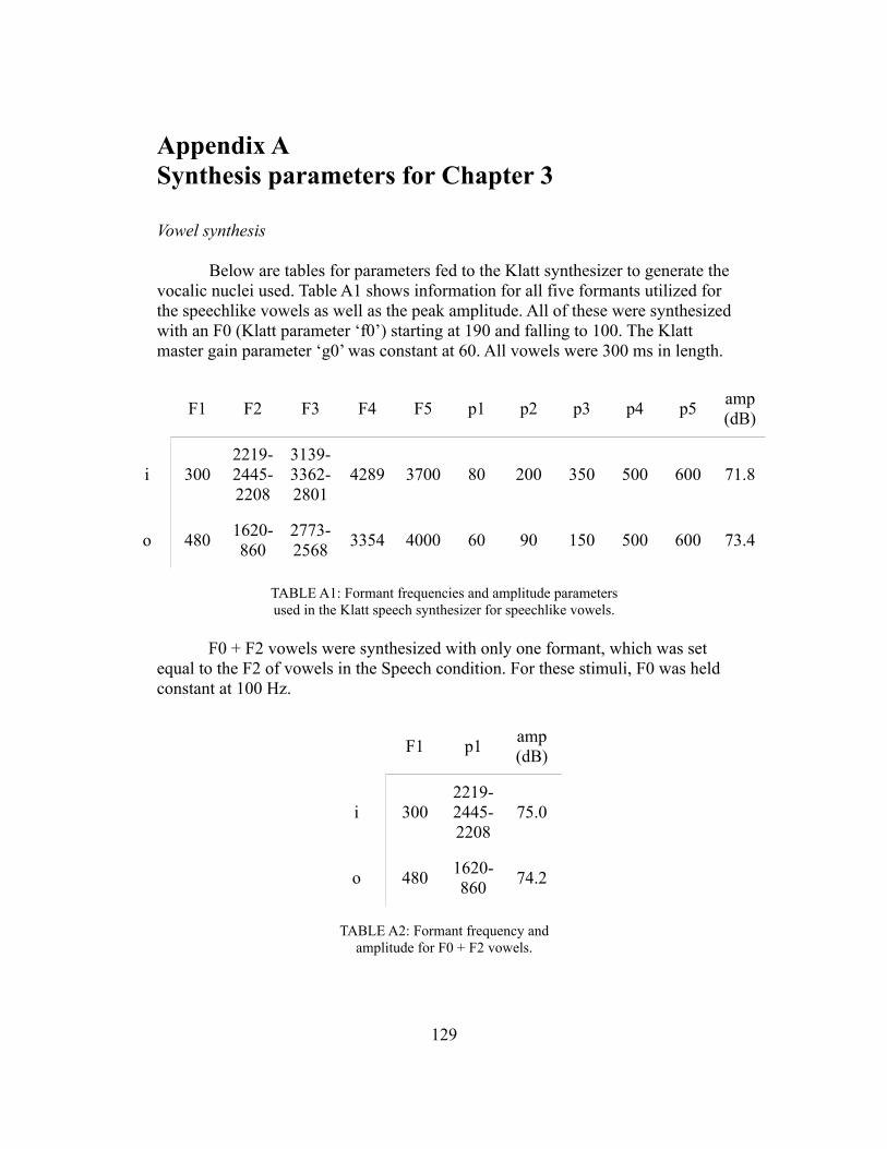
Appendix ASynthesis parameters for Chapter 3

Vowel synthesis

Below are tables for parameters fed to the Klatt synthesizer to generate the vocalic nuclei used. Table A1 shows information for all five formants utilized for the speechlike vowels as well as the peak amplitude. All of these were synthesized with an F0 (Klatt parameter ‘f0’) starting at 190 and falling to 100. The Klatt master gain parameter ‘g0’ was constant at 60. All vowels were 300 ms in length.

F1 F2 F3 F4 F5 p1 p2 p3 p4 p5 amp (dB)

i 3002219-2445-2208

3139-3362-2801

4289 3700 80 200 350 500 600 71.8

o 480 1620-860

2773-2568 3354 4000 60 90 150 500 600 73.4

TABLE A1: Formant frequencies and amplitude parametersused in the Klatt speech synthesizer for speechlike vowels.

F0 + F2 vowels were synthesized with only one formant, which was set equal to the F2 of vowels in the Speech condition. For these stimuli, F0 was held constant at 100 Hz.

F1 p1 amp (dB)

i 3002219-2445-2208

75.0

o 480 1620-860 74.2

TABLE A2: Formant frequency andamplitude for F0 + F2 vowels.

129

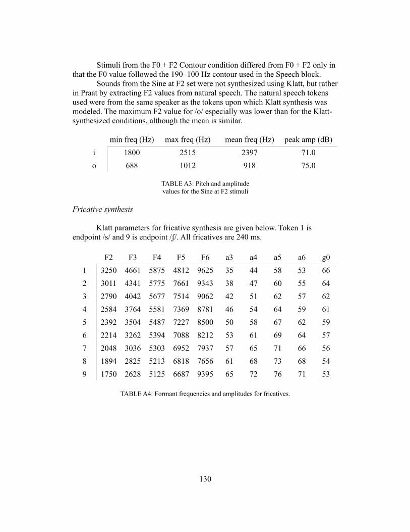
Stimuli from the F0 + F2 Contour condition differed from F0 + F2 only in that the F0 value followed the 190–100 Hz contour used in the Speech block.

Sounds from the Sine at F2 set were not synthesized using Klatt, but rather in Praat by extracting F2 values from natural speech. The natural speech tokens used were from the same speaker as the tokens upon which Klatt synthesis was modeled. The maximum F2 value for /o/ especially was lower than for the Klatt-synthesized conditions, although the mean is similar.

min freq (Hz) max freq (Hz) mean freq (Hz) peak amp (dB)i 1800 2515 2397 71.0o 688 1012 918 75.0

TABLE A3: Pitch and amplitudevalues for the Sine at F2 stimuli

Fricative synthesis

Klatt parameters for fricative synthesis are given below. Token 1 is endpoint /s/ and 9 is endpoint /$/. All fricatives are 240 ms.

F2 F3 F4 F5 F6 a3 a4 a5 a6 g01 3250 4661 5875 4812 9625 35 44 58 53 662 3011 4341 5775 7661 9343 38 47 60 55 643 2790 4042 5677 7514 9062 42 51 62 57 624 2584 3764 5581 7369 8781 46 54 64 59 615 2392 3504 5487 7227 8500 50 58 67 62 596 2214 3262 5394 7088 8212 53 61 69 64 577 2048 3036 5303 6952 7937 57 65 71 66 568 1894 2825 5213 6818 7656 61 68 73 68 549 1750 2628 5125 6687 9395 65 72 76 71 53

TABLE A4: Formant frequencies and amplitudes for fricatives.

130

Appendix BAdditional figures for Chapter 6

Numbers of tokens in the training set

Phone Count

[i] 1103[e(] 756[æ] 1449[!] 1022[&] 534

[o)] 689[+] 319[,] 719[-] 145[w] 296[m] 153[n] 221

total 7406

131

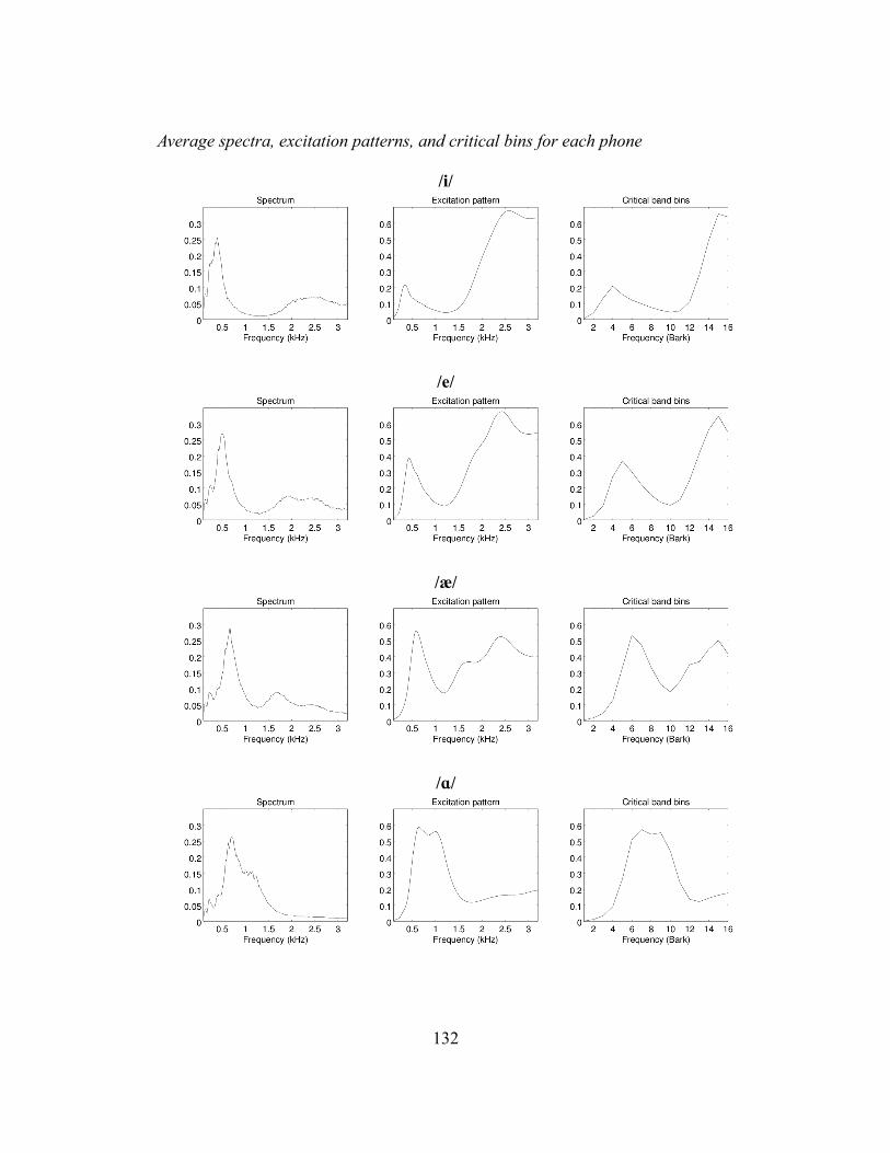
Average spectra, excitation patterns, and critical bins for each phone

/i/

/e/

/æ/

/!/

132

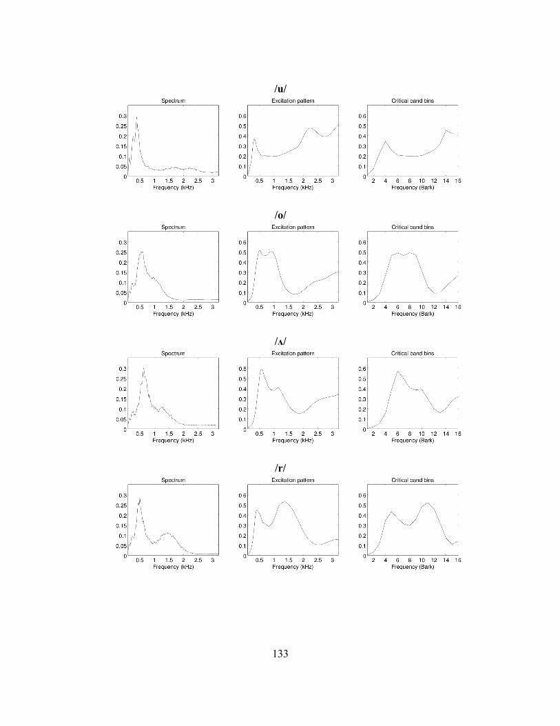
/u/

/o/

/"/

/r/

133

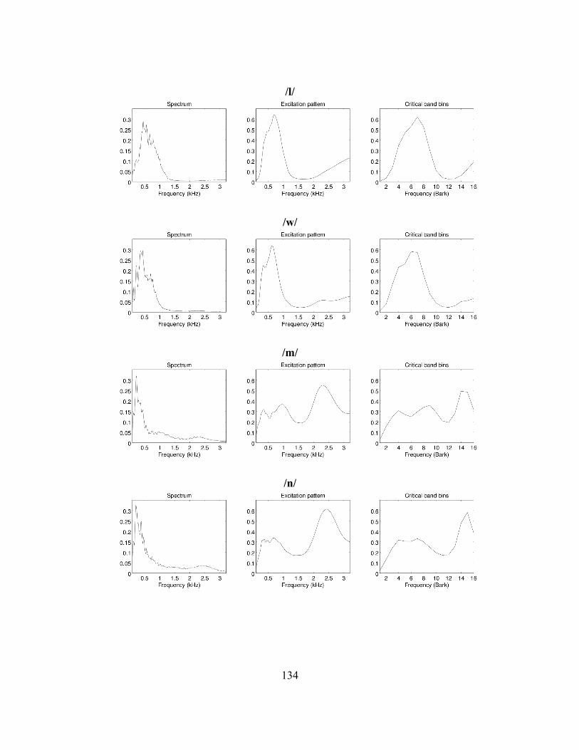
/l/

/w/

/m/

/n/

134

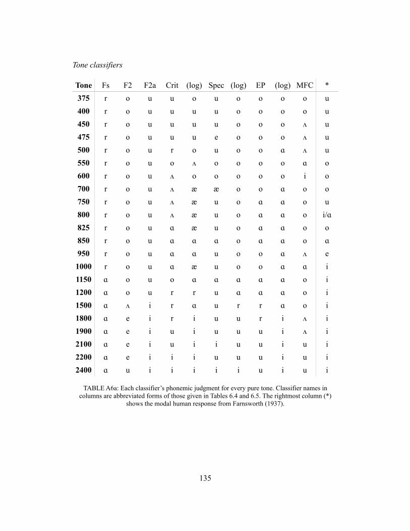
Tone classifiers

Tone Fs F2 F2a Crit (log) Spec (log) EP (log) MFC *375 r o u u o u o o o o u400 r o u u u u o o o o u450 r o u u u u o o o + u475 r o u u u e o o o + u500 r o u r o u o o ! + u550 r o u o + o o o o ! o600 r o u + o o o o o i o700 r o u + æ æ o o ! o o750 r o u + æ u o ! ! o u800 r o u + æ u o ! ! o i/!825 r o u ! æ u o ! ! o o850 r o u ! ! ! o ! ! o !950 r o u ! ! u o o ! + e1000 r o u ! æ u o o ! ! i1150 ! o u o ! ! ! ! ! o i1200 ! o u r r u ! ! ! o i1500 ! + i r ! u r r ! o i1800 ! e i r i u u r i + i1900 ! e i u i u u u i + i2100 ! e i u i i u u i u i2200 ! e i i i u u u i u i2400 ! u i i i i i u i u i

TABLE A6a: Each classifier’s phonemic judgment for every pure tone. Classifier names in columns are abbreviated forms of those given in Tables 6.4 and 6.5. The rightmost column (*)

shows the modal human response from Farnsworth (1937).

135

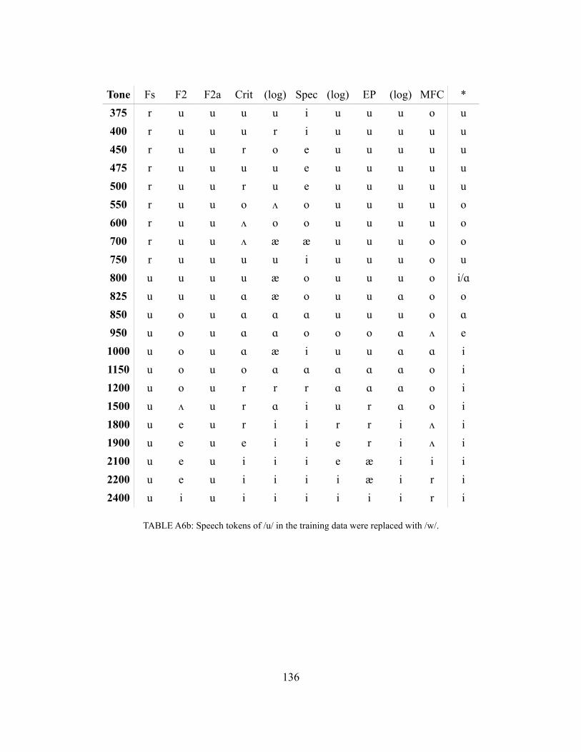
Tone Fs F2 F2a Crit (log) Spec (log) EP (log) MFC *375 r u u u u i u u u o u400 r u u u r i u u u u u450 r u u r o e u u u u u475 r u u u u e u u u u u500 r u u r u e u u u u u550 r u u o + o u u u u o600 r u u + o o u u u u o700 r u u + æ æ u u u o o750 r u u u u i u u u o u800 u u u u æ o u u u o i/!825 u u u ! æ o u u ! o o850 u o u ! ! ! u u u o !950 u o u ! ! o o o ! + e1000 u o u ! æ i u u ! ! i1150 u o u o ! ! ! ! ! o i1200 u o u r r r ! ! ! o i1500 u + u r ! i u r ! o i1800 u e u r i i r r i + i1900 u e u e i i e r i + i2100 u e u i i i e æ i i i2200 u e u i i i i æ i r i2400 u i u i i i i i i r i

TABLE A6b: Speech tokens of /u/ in the training data were replaced with /w/.

136