Embed Size (px)
Citation preview
Review of Economic Studies (2010) 77, 1 192-1230 0034-6527/10/0041 101 1$02.00 © 2009 The Review of Economic Studies Limited doi: 10.1 1 1 l/j.l467-937X.2009.00589.x
Accounting for Incomplete Pass-Through
EMI NAKAMURA Columbia University
and
DAWIT ZEROM California State University, Fullerton
First version received May 2007; final version accepted August 2009 (Eds.)
Recent theoretical work has suggested a number of potentially important factors in causing incomplete pass-through of exchange rates to prices, including markup adjustment, local costs and barriers to price adjustment. We empirically analyse the determinants of incomplete pass-through in the coffee industry. The observed pass-through in this industry replicates key features of pass-through documented in aggregate data: prices respond sluggishly and incompletely to changes in costs. We use microdata on sales and prices to uncover the role of markup adjustment, local costs and barriers to
price adjustment in determining incomplete pass-through using a structural oligopoly model that nests all three potential factors. The implied pricing model explains the main dynamic features of short and
long-run pass-through. Local costs reduce long-run pass-through (after six quarters) by 59% relative to a Constant Elasticity of Substitution benchmark. Markup adjustment reduces pass-through by an additional 33%, where the extent of markup adjustment depends on the estimated "super-elasticity" of demand. The estimated menu costs are small (0.23% of revenue) and have a negligible effect on
long-run pass-through but are quantitatively successful in explaining the delayed response of prices to costs. We find that delayed pass-through in the coffee industry occurs almost entirely at the wholesale rather than the retail level.
1. INTRODUCTION
A substantial body of empirical work documents that exchange rate movements lead to less than proportional increases in traded goods prices; and much of the price response occurs with a substantial delay (Engel, 1999; Parsley and Wei, 2001; Goldberg and Campa, 2006).
* In other words, exchange rate pass-through into prices is delayed and incomplete.
Recent theoretical work has suggested a number of potentially important factors in
explaining incomplete pass-through. First, in oligopolistic markets, the response of prices to changes in costs depends both on the curvature of demand and on the market structure (Dornbusch, 1987; Knetter, 1989; Bergin and Feenstra, 2001; Atkeson and Burstein, 2008). Second, local costs may play an important role in determining pass-through (Sanyal and Jones, 1982; Burstein, Neves and Rebelo, 2003; Corsetti and Dedola, 2005). Local costs drive a
wedge between prices and imported costs that is unresponsive to exchange rate fluctuations. As a consequence, if local costs are large, even a substantial increase in the price of an imported
1. See also Frankel, Parsley and Wei (2005) and Parsley and Popper (2009).
1192
This content downloaded from 128.59.160.114 on Tue, 16 Jun 2015 22:14:16 UTCAll use subject to JSTOR Terms and Conditions

NAKAMURA & ZEROM ACCOUNTING FOR INCOMPLETE PASS-THROUGH 1 193
factor of production could have little impact on marginal costs. Third, price rigidity and other dynamic factors have the potential to contribute to incomplete pass-through (Giovannini, 1988; Kasa, 1992; Devereux and Engel, 2002; Bacchetta and van Wincoop, 2003).
We study pass-through in the coffee industry. Coffee is the world's second most traded com- modity after oil. Over the past decade, coffee commodity prices have exhibited a remarkable amount of volatility. However, retail and wholesale coffee prices have responded sluggishly and incompletely to changes in imported commodity costs, an important feature of the aggregate evidence.2
The response of prices to changes in costs is intimately related to the response of prices to exchange rates. Indeed, the equations used to estimate the response of prices to exchange rates are derived from equations that relate prices to marginal costs. In standard exchange rate pass-through regressions, foreign inflation is used to proxy for marginal costs, and prices are regressed separately on costs and exchange rates. The coffee market is an ideal laboratory to study how costs pass through into prices because a large fraction of marginal costs are observ- able for this industry. Coffee commodity costs are, moreover, buffeted by large weather shocks. This makes price responses easier to interpret than price movements related to exchange rates. Exchange rate movements may be closely linked to monetary factors that have a direct effect on prices, at least in the long run (Corsetti, Dedola and Leduc, 2008; Bouakez and Rebei, 2008).3
We find that for both retail and wholesale prices a 1% increase in coffee commodity costs leads to an increase in prices of approximately a third of a per cent over the subsequent six quarters (we refer to this as long-run pass-through). More than half of the price adjustment occurs with a delay of one quarter or more. By wholesale prices, we mean the prices charged by coffee roasters like Folgers and Maxwell House to retailers. (We will sometimes also refer to these wholesale prices as manufacturer prices.)
Using reduced form regressions, we show that delayed pass-through in this industry occurs almost entirely at the wholesale level. This evidence suggests that, to the extent that barriers to price adjustment contribute to delayed pass-through in this industry, it is wholesale price rigidity that matters. Recent research on price dynamics has focused on price rigidity at the retail level, partly because retail price data are more readily available to researchers. The find- ing that, at least in the coffee industry, the majority of incomplete pass-through arises at the level of wholesale prices indicates that studies that focus exclusively on retail prices may be incomplete in an important way.4
We document substantial rigidity in coffee prices at both the wholesale and the retail level: manufacturer prices of ground coffee adjust on average 1.3 times per year, whereas retail prices excluding sales adjust on average 1.5 times per year over the time period we consider. The frequency of wholesale price adjustment is highly correlated with commodity cost volatility: wholesale prices adjust substantially more frequently during periods of high commodity cost volatility. Goldberg and Verbo ven (2001) similarly document an important role for wholesale price rigidity in the beer market using data from a large US supermarket chain.
We build a structural model of the coffee industry and investigate its success in explaining the facts about pass-through. We begin by estimating a model of demand for coffee. The coffee
2. This has generated considerable public interest in coffee markets. In 1955, 1977 and 1987, the US Congress launched inquiries into the pricing practices of coffee manufacturers.
3. An important strand of the international economics literature seeks to understand incomplete pass-through to the prices of imported inputs "at the dock". We focus instead on incomplete pass-through at the manufacturer and retail level, where imported inputs are an intermediate good.
4. Retailer-manufacturer interactions may also play an important role in determining manufacturer pricing behaviour (e.g. Hellerstein, 2008; Villas Boas, 2007; Burstein et al., 2003; Corsetti and Dedola, 2005).
© 2009 The Review of Economic Studies Limited
This content downloaded from 128.59.160.114 on Tue, 16 Jun 2015 22:14:16 UTCAll use subject to JSTOR Terms and Conditions

1 194 REVIEW OF ECONOMIC STUDIES
market, like most markets, is best described as a differentiated products market. The main dif- ficulty of estimating demand curves in a differentiated products industry is that an unrestricted specification of the dependence of demand on prices leads to an extremely large number of free parameters. It is therefore useful to put some structure on the nature of demand. We do this by specifying a discrete choice model of demand (McFadden, 1974). This type of structural model places restrictions on the cross-price elasticities by assuming utility maximizing behaviour, thereby resulting in a substantially more parsimonious model. We follow Berry, Levinsohn and Pakes (1995) in estimating a random coefficients model with unobserved product characteris- tics. An advantage of the coffee industry in estimating the demand system is that coffee prices are buffeted by large exogenous shocks to supply in the form of weather shocks to coffee pro- ducing countries. We use these weather shocks as instruments to identify the price elasticity of demand.
We combine this demand model with a structural model of the supply side of the coffee industry. We fix the number of firms and the products produced by the firms to match the observed industry structure. We account for the observed degree of price rigidity by assuming that firms must pay a "menu cost" to adjust their prices. According to this model, firms face a fixed cost of price adjustment that leads them to adjust their prices infrequently. The barriers to price adjustment imply that the model is a dynamic game. We then analyse the equilibrium response of prices to costs in a Markov perfect equilibrium of this model. Incorporating price rigidity in the model is crucial both because of its impact on short-run dynamics and because ignoring these factors could otherwise bias our estimates of the role of local costs and markup adjustment (Engel, 2002).
We find that the dynamic pricing model, estimated using panel data on prices and market shares, replicates the main dynamic features of pass-through in the data both in the short-run and in the long-run. We use the model to determine the role of local costs, markup adjust- ment and menu costs in long-run pass-through. We do this by comparing our baseline dynamic model with successively simpler models. We find that local costs reduce pass-through by 59% relative to a Constant Elasticity of Substitution (CES) benchmark, whereas markup adjustment reduces pass-through by an additional 33%.5 Menu costs have a negligible effect on long-run pass-through after six quarters because of the high persistence of marginal costs, although they play an important role in explaining short-run pricing dynamics. Our conclusions underscore the need to allow for additional channels of incomplete pass-through in the large literature in international macroeconomics in which rigid prices are the main source of imperfect adjustment of prices to costs.6
In comparing the model with the data, we emphasize three main features of our results. First, in the long-run, markup adjustment in response to cost shocks is substantial: firms are estimated to compress their gross margins on average by 1/3 in response to a marginal cost increase. This implies that a 1% increase in coffee commodity costs leads to a "long-run" pass-through into prices of approximately a third of a per cent over the subsequent six quarters, despite a much larger fraction of marginal costs being accounted for by green bean coffee. Klenow and Willis (2006) coin the term "super-elasticity" of demand for the percentage change in the price elasticity for a given percentage increase in prices and show that it is a key determinant of how prices respond to costs in macroeconomic models. The super-elasticity is, therefore, a
5. These results echo the findings of Goldberg and Verbo ven (2001) for the European car market, as well as the findings of Burstein, Eichenbaum and Rebelo (2005) for the behaviour of tradable goods prices following large devaluations in terms of the large role played by local costs. Our findings are also consistent with the results of Lubik and Schorfheide (2005).
6. See, for example, Engel (2002) for a discussion of this literature.
© 2009 The Review of Economic Studies Limited
This content downloaded from 128.59.160.114 on Tue, 16 Jun 2015 22:14:16 UTCAll use subject to JSTOR Terms and Conditions

NAKAMURA & ZEROM ACCOUNTING FOR INCOMPLETE PASS-THROUGH 1 195
quantitative measure of the curvature of demand. While the Dixit-Stiglitz model (Dixit and Stiglitz, 1977) implies a super-elasticity of demand of 0, we estimate a median super-elasticity of demand of 4.64, generating a substantial motive for markup adjustment.7
Second, the menu cost model parameterized to fit the overall frequency of price change is quantitatively successful in matching the short-run dynamics of pass-through. Most of the price adjustment occurs in the quarters after the initial change in costs. The menu costs imply a substantial amount of price rigidity: prices adjust only every 9 or 10 months. However, menu costs are found to play a negligible role in explaining long-run pass-through after six quarters. In theory, strategic complementarities in pricing among firms can substantially amplify the delays in price adjustment associated with price rigidity. We find, however, that these effects are quantitatively small for our estimated model of demand.
Third, our analysis strongly favours the dynamic menu cost model over a pricing model in which firms set prices purely according to a fixed schedule as in the Taylor model (Taylor, 1980) or change prices with a fixed probability as in the Calvo model (Calvo, 1983). The central prediction of the menu cost model is that price adjustments occur more frequently in periods when marginal costs change substantially. While this is an important prediction of the menu cost model, it has been difficult to study given the difficulty of observing marginal costs. This prediction of the model is borne out strongly by the data. There is a strong positive relationship between turbulence in the coffee commodity market and the frequency of price change in a given year. Moreover, the observed price rigidity and delayed response of prices to costs can be explained by a plausibly small magnitude of adjustment costs (0.23% of revenue). Small menu costs are found to generate a large amount of price rigidity both because of relatively inelastic demand and because local costs account for a large fraction of marginal costs.
It is worth emphasizing that neither the model's fit to the dynamics of pass-through nor its fit to the timing of price adjustments is "guaranteed" by the estimation procedure: the estimation procedure uses information on long-run average prices, demand and frequency of price change but does not make use of the empirical evidence on pass-through or the timing of price adjustments.
The basic approach we use to study pass-through in this industry builds on recent work by Goldberg and Verbo ven (2001) and Hellerstein (2008). These papers provide detailed models of pricing in particular industries and analyse their models' implications for pass-through. In particular, Hellerstein (2008) introduces a novel decomposition of the sources of incomplete pass-through into non-traded costs and markup adjustment. These analyses have focused on the contemporaneous response of prices to changes in costs. However, the delayed response of prices to costs suggests that dynamic factors are also important in explaining pass-through and may affect existing empirical results. Engel (2002) argues that Goldberg and Verboven (2001) overestimate the role of local costs because they do not allow for price rigidity.
This paper extends the existing static models to incorporate additional empirical facts about delayed and incomplete pass-through. Goldberg and Hellerstein (2007) carry out a closely related study of the role of price rigidity in pass-through in the beer market but approximate the firms' pricing policies using a static model. In contrast, we study firm pricing policies in a dynamic framework. The menu cost pricing model in this paper builds on Slade (1998, 1999) and Aguirregabiria (1999) who incorporate menu costs into industrial organization models of price adjustment to estimate the barriers to price adjustment. Another closely related paper is Kano (2006) that also solves for the Markov perfect equilibrium of a dynamic menu cost model
7. See also Bulow and Pfleiderer (1983) for a discussion of how the shape of the demand curve affects the response of prices to costs.
© 2009 The Review of Economic Studies Limited
This content downloaded from 128.59.160.114 on Tue, 16 Jun 2015 22:14:16 UTCAll use subject to JSTOR Terms and Conditions
1 196 REVIEW OF ECONOMIC STUDIES
using numerical methods. More broadly, this paper is related to a large empirical literature on cost pass-through as well as a growling literature on state-dependent pricing models solved using numerical methods.8 Bettendorf and Verboven (2000) study the relationship between Dutch coffee prices and commodity costs in a static oligopoly model and find similar results on the magnitude of non-coffee bean costs.
One issue that arises in this type of industry-based analysis is the extent to which conclu- sions based on one particular industry can be extended to understand pricing dynamics in other industries. The major players in this industry, Proctor & Gamble, Kraft and Sara Lee, are some of the world's largest consumer packaged goods companies, selling products in a diverse range of markets, from beauty products and pharmaceuticals to household cleaning products and pack- aged foods. Studying the behaviour of large consumer packaged goods companies in the coffee market may give insights into their pricing behaviour in other markets as well. Economy-wide studies of price rigidity suggest, furthermore, that the extent of price rigidity in the coffee mar- ket is typical of other industries (Nakamura and Steinsson, 2008). Moreover, the coffee market provides a close-up study of price dynamics at both the retail and the wholesale level. The relationship between retail and wholesale prices is important to understanding price dynamics in general because retailers play an important role in large swaths of the economy, particularly food, clothing and household furnishings, which account for more than 30% of US consumption. Finally, in relating our analysis to the literature on exchange rate pass-through, an important similarity between coffee commodity costs and exchange rates is that both variables are highly persistent. The persistence and volatility of cost shocks turns out to matter substantially for our conclusions regarding both long-run pass-through and the magnitude of menu costs.
However, it is important to note that relative to other industries, imported costs are likely to constitute a particularly large fraction of marginal costs in the coffee industry. Indeed, we selected the coffee industry for analysis in part because of the disproportionate share of marginal costs accounted for by imported intermediate goods (coffee beans).9 Moreover, because coffee costs are highly correlated across firms, different coffee producers' incentives to adjust their prices tend to be coordinated. In markets where firms face disparate cost shocks, the incentive for a firm to compress its markup in response to a cost increase may be greater. This may contribute to greater pricing-to-market in other industries than what we observe in the coffee market. Finally, we abstract from the notion that firms may respond differently to movements in exchange rates and costs because of a "cognitive divide" in decision-making based on domes- tic versus foreign variables, that could arise in models of limited information capacity (e.g. Mackowiak and Wiederholt, 2009).
The paper proceeds as follows. Section 2 provides an overview of the data used in the paper. Section 3 presents stylized facts about price adjustment in the coffee industry. Section 4 describes the demand model. Section 5 presents estimates of markups and local costs. Section 6 presents the menu cost oligopoly model. Section 7 presents simulation results for the dynamic model and compares them with the data. Section 8 presents a number of counterfactual simu- lations. Section 9 concludes.
8. In the cost pass-through literature, see Kadiyali (1997), Gron and Swenson (2000) and Levy et al. (2002). See also Bettendorf and Verboven (2000) and the references therein for specific analyses of coffee prices in various countries. A recent example of a numerical state-dependent pricing model in the international economics literature is Roden and Wilander (2006).
9. Consumer goods are sometimes imported in finished form, implying a very high fraction of imported intermediate inputs. Most imported products are, however, intermediate or investment goods.
© 2009 The Review of Economic Studies Limited
This content downloaded from 128.59.160.114 on Tue, 16 Jun 2015 22:14:16 UTCAll use subject to JSTOR Terms and Conditions

NAKAMURA & ZEROM ACCOUNTING FOR INCOMPLETE PASS-THROUGH 1 197
2. DATA ON PRICES AND COSTS
We pull together data on prices and costs from a number of sources to develop our model of the coffee industry. We use data on prices and sales from two industry sources. Our source for retail price and sales data is monthly AC Nielsen data. These data are market-level average prices and sales for the period 2000-2004. We use these data to construct series on retail prices and market shares.10
We use wholesale price data from PromoData. PromoData collects data on manufacturer prices for packaged foods from grocery wholesalers. PromoData collects its information from the largest grocery wholesaler in a given market but does not identify the wholesaler for confidentiality reasons. These data provide the price per case charged by the manufacturer to the wholesaler for a particular Universal Product Code (UPC) in a particular week (in contrast to the retail data which are market-level averages). The data start in January 1997 and end in December 2005. Data are available for 31 of the 50 retail markets, for the leading products in each market.
A limitation of this data source for wholesale prices is that not all retailers purchase from grocery wholesalers. In a recent report by the Brazil Information Center (2002), about half of 20 large US retailers interviewed reported using grocery wholesalers, although the fraction was lower among the largest supermarkets in this group. In general, the price quoted to a grocery wholesaler is non-negotiable, and the product is delivered directly to the wholesaler's warehouse. The grocery wholesaler then resells the product to a supermarket.
The wholesale price data contain information on both base prices and "trade deals". Trade deals are discounts offered to the grocery wholesalers to encourage promotions, and often carry special conditions such as proof that a promotion has been carried out to redeem the discount. The cost pass-through regressions we present are for prices including trade deals, although our results on pass-through are similar both including and excluding trade deals.
The commodity price data are based on commodity prices on the New York Physicals market collected by the International Coffee Organization (ICO). We focus on price responses to a "composite commodity index" constructed as a weighted average of the commodity prices for Colombian Mild Arabicas, Other Mild Arabicas, Brazilian and Other Natural Arabicas and Robustas. We weight the commodity prices for the different varieties based on the average composition of US coffee consumption from Lewin, Giovannucci and Varangis (2004) over the years 1993-2002. These weights have remained relatively stable over the sample period. Although it would be more ideal to have product-specific weights on the different coffee vari- eties, we believe this would have little impact on our results given the high covariances across their prices. We adjust the commodity price for the fact that roasted green coffee beans lose about 19% of their weight during the roasting process.
3. COST PASS-THROUGH REGRESSIONS
Let us begin by looking at the relative movements of coffee prices and costs over the past decade.11 Figure 1 presents a graph of average retail, wholesale and commodity prices in US
10. AC Nielsen collects prices from cooperating supermarkets with at least $2 million in sales. Sales by super- centers, such as Walmart and Target, are not covered in the data. The 50 AC Nielsen markets, which are generally considerably larger than cities, span almost the entire continental United States. To estimate the demand model, we also matched Current Population Survey (CPS) demographic data to the ACN market areas using a concordance between AC Nielsen markets and MSA/county code information provided by AC Nielsen.
1 1 . This section draws heavily on the analysis in Leibtag et al. (2005).
© 2009 The Review of Economic Studies Limited
This content downloaded from 128.59.160.114 on Tue, 16 Jun 2015 22:14:16 UTCAll use subject to JSTOR Terms and Conditions

1 198 REVIEW OF ECONOMIC STUDIES
Figure 1
Retail, wholesale and commodity prices The roasted coffee retail and ground coffee manufacturer prices are average prices from the Bureau of Labor Statistics (the "ground coffee" retail price index and the "roasted coffee" wholesale price index). The Arabica 12 month futures price is from the New York Board of Trade. The coffee commodity index is the "composite commodity index" discussed in Section 2. The gap in the retail price series from November 1998 to September 1999 arises from missing data.
dollars per ounce. To be clear about terminology, we shall refer to the price charged by super- markets to consumers as the retail price, the price charged by coffee roasters such as Folgers and Maxwell House to grocery wholesalers as the wholesale price, and the price of green bean coffee on the New York market as the commodity cost.
The vast majority of coffee sold in the United States is imported in the form of green bean coffee (the largest coffee producing countries are Brazil, Colombia and Vietnam). Coffee manufacturers roast, grind, package and deliver the coffee to the American market. Green bean coffee prices were highly volatile over the period we study, losing almost two-thirds of their value between 1997 and 2002. Most of the volatility in commodity costs arises from weather conditions in coffee producing countries, planting cycles and new players in the coffee market. Because coffee commodity prices are quoted in US dollars, commodity prices have also been affected by the rise and fall of the value of the US dollar.
We document three facts about prices and costs in the coffee market: (1) the pass-through of coffee commodity prices to retail and wholesale coffee prices, (2) the response of retail to wholesale coffee prices and (3) the extent of price rigidity in wholesale prices in the coffee industry. First, we document the dynamics of the relationship between prices and costs. Figure 1 shows that retail and wholesale prices tracked commodity prices closely over this period. The close relationship between prices and commodity costs is not surprising given the large role of green bean coffee in ground coffee production. Industry estimates suggest that green bean coffee
© 2009 The Review of Economic Studies Limited
This content downloaded from 128.59.160.114 on Tue, 16 Jun 2015 22:14:16 UTCAll use subject to JSTOR Terms and Conditions
NAKAMURA & ZEROM ACCOUNTING FOR INCOMPLETE PASS-THROUGH 1 199
accounts for more than half of the marginal costs of coffee production (Yip and Williams, 1985). To quantify this relationship, we estimate the following standard pass-through regression,
6 4
Mogpljmt = a + J2bkA'ogCt-k + J2dk(lk + é' (1) k=' k='
where / = r, tu, A log prjmt is the log retail price change of product j in market m, A log pjmt is the corresponding log wholesale price change, A log Ct-k is the log commodity cost index, qt is a quarter of the year dummy, a, bk and dk are parameters and € is a mean zero error term. The wholesale price series includes trade deals; the results excluding trade deals are extremely similar.12 The coefficients bk may be interpreted as the percentage change in prices associated with a given percentage change in commodity costs k quarters ago. The empirical model follows the approach of Goldberg and Campa (2006). The model is motivated by the fact that, as in Goldberg and Campa (2006), the regressor is highly persistent: a Dickey-Fuller test for the hypothesis of a unit root in commodity prices cannot be rejected at a 5% significance level. Goldberg and Campa (2006) define the long-run rate of pass-through in this model as the sum of the coefficients XjLi bk- We selected the number of lags included in the regression such that adding additional lags does not change the estimated long-run rate of pass-through. We estimate the model using the retail and wholesale price data described in Section 2, for quarterly changes in prices and costs over the 2000-2005 period.13
Table 1 presents the results of the pass-through regression for retail and wholesale prices. We present estimates from two types of pass-through regressions. Standard errors are clustered by unique product and market to allow for arbitrary serial correlation. Columns 1 and 2 of Table 1 present the results of the standard pass-through regression (1). The results reflect a substantial amount of incomplete pass-through in percentage terms. The estimated long-run pass-through elasticity is 0.252 for retail prices and 0.262 for wholesale prices. In other words, a 1% increase in commodity costs eventually leads to only about a quarter of a percent increase in coffee prices. We do not find robust evidence that prices systematically react asymmetrically to price increases or decreases. Table 1 also documents that there is a substantial delay in the response of prices to commodity costs. For both retail and wholesale prices, more than half of the adjustment to a change in costs occurs in the period after the cost shock.14
Columns 3 and 4 of Table 1 present the results of the pass-through regression (1) in levels rather than logs. For this specification, the long-run pass-through of retail prices to commod- ity costs is 0.916, whereas the long-run pass-through to wholesale prices is 0.852. Thus, a 1 cent increase in commodity prices leads to slightly less than a 1 cent increase in prices. The difference between the regressions in levels and logs is explained by the substantial wedge between observed prices and commodity costs, which implies that a 1 cent change corresponds
12. Trade deals are slightly more common when commodity costs are low. The effect is, however, quantitatively small: an increase in green bean coffee costs by 1 cent lowers the frequency of trade deals by about 0.2 percentage points; the size of trade deals is not correlated in a statistically significant way with commodity costs.
13. An alternative approach would be to estimate a panel error correction model. We cannot reject the null of no cointegration of coffee prices and coffee bean costs in aggregate data over the time period we consider. Nevertheless, as a robustness check, we also estimated a number of specifications that allow for a cointegrating relationship between prices and green bean coffee costs (reported in the working paper version of this paper) with broadly similar results.
14. These statistics are for retail prices including temporary sales. A 1 cent per ounce increase in commodity costs is associated with a 0.03 cent decrease in the difference between base prices (excluding sales) and net prices (including sales), about 3% of the overall pass-through, based on a fixed effects regression of the difference between base and net prices on commodity costs and quarter dummies. According to this metric, temporary sales contribute little to overall pass-through.
© 2009 The Review of Economic Studies Limited
This content downloaded from 128.59.160.114 on Tue, 16 Jun 2015 22:14:16 UTCAll use subject to JSTOR Terms and Conditions

1200 REVIEW OF ECONOMIC STUDIES
TABLE 1 Pass-through regressions
Log specification Levels specification
Variable Retail Wholesale Retail Wholesale
A Commodity cost (0 0.063(0.013) 0.115(0.018) 0.142(0.040) 0.218(0.061) A Commodity cost (t - 1) 0.104(0.008) 0.169(0.013) 0.446(0.024) 0.520(0.043) A Commodity cost (f - 2) 0.013 (0.007) -0.010 (0.010) 0.016 (0.019) 0.029 (0.028) A Commodity cost (/ - 3) 0.031 (0.006) -0.016 (0.009) 0.080 (0.018) 0.004 (0.026) A Commodity cost (t - 4) 0.048 (0.007) 0.007 (0.013) 0.144 (0.018) 0.023 (0.030) A Commodity cost it - 5) 0.007 (0.006) 0.025 (0.01 1) 0.070 (0.017) 0.067 (0.031) A Commodity cost (t - 6) -0.015 (0.008) -0.026 (0.012) 0.017 (0.021) -0.009 (0.029) Constant 0.033 (0.003) -0.004 (0.003) 0.007 (0.0004) 0.001 (0.0005) Long-run pass-through 0.252 (0.007) 0.262 (0.018) 0.916 (0.023) 0.852 (0.052) Number of observations 40,129 2867 40,129 2867 /?-squared 0.079 0.141 0.088 0.134
Notes: The retail price variable is the change in the UPC-level retail price per ounce in a particular US market over a quarter. The wholesale price variable is the change in the wholesale price per ounce (including trade deals) of a particular UPC in a particular US market over a quarter. The standard errors are clustered by unique product and market to allow for arbitrary serial correlation in the error term for a given product. The data cover the period 2000-2005.
to a substantially smaller percentage change in prices than costs. This alternative specification of the pass-through regression begs the question of whether it might be more relevant to con- sider cent-for-cent pass-through as a benchmark for "complete" pass-through as opposed to a pass-through elasticity of 1. However, a pass-through elasticity of 1 is an appealing benchmark both because it arises in the workhorse Dixit-Stiglitz model (absent local costs) and because it is only possible to calculate pass-through elasticities (rather than levels) using standard data sources on price indices.
One might be concerned that long-term contracts for purchasing green bean coffee imply that the average purchasing price of coffee manufacturers may differ from the coffee commodity price. However, this concern ignores the fact that in an economic model, firms' prices respond to marginal costs rather than accounting costs. Although hedging contracts affect the firm's total costs, they do not affect its marginal costs, so long as the firm is always on the margin of buying or selling at the observed commodity cost.
Second, we document the responsiveness of retail prices to manufacturer prices. This analysis investigates to what extent delays in pass-through occur at the wholesale versus the retail level. This issue matters both for how we model price adjustment behaviour, and what data are most relevant for parameterizing the model. In order to analyse this issue, we consider the following regression of retail prices on wholesale prices,
2 4
¿P'jmt = O? + E ßk APjmt-k + E ri* + «. O) k=0 k='
where ctr, ßrk and yrk are parameters, and e is a mean zero error term. The wholesale price data are likely to be a noisy proxy for the wholesale costs faced by any particular retailer. To avoid attenuation bias, we estimate this equation by instrumental variables regression with commodity costs as instruments.15 Table 2 reports the results of this regression. The estimated
15. The instruments we use are current changes in the commodity cost index and 12 month Arabica futures prices as well as six lags of these variables.
© 2009 The Review of Economic Studies Limited
This content downloaded from 128.59.160.114 on Tue, 16 Jun 2015 22:14:16 UTCAll use subject to JSTOR Terms and Conditions
NAKAMURA & ZEROM ACCOUNTING FOR INCOMPLETE PASS-THROUGH 1201
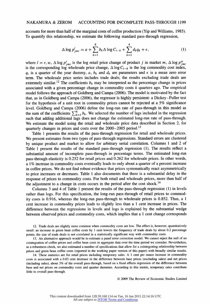
TABLE 2 IV regression of retail on wholesale prices
Retail prices
A Wholesale price (f) 0.958 (0.131) A Wholesale price (t - 1) -0.050 (0.180) A Wholesale price (t - 2) -0.027 (0.129) Constant 0.005 (0.001) Quarter dummies Yes Number of observations 2792 Instruments Commodity costs
Notes: The dependent variable is the change in the UPC- level monthly average of the retail price per ounce in a particular US market over a quarter. The wholesale price variable is the change in the wholesale price per ounce (including trade deals) of a particular UPC in a particular US market over a quarter. The standard errors are clustered by unique product and market to allow for arbitrary serial correlation in the error term. The data cover the period 2000-2005. Wholesale prices are instrumented for by current changes in commodity costs and Arabica futures as well as six lags of these variables.
pass-through coefficient on contemporaneous changes in wholesale prices is 0.958, with small and insignificant coefficients on the lagged wholesale price changes. This regression indicates that retail prices respond immediately and approximately cent-for-cent to changes in wholesale prices associated with cost shocks, indicating that almost all of the delays in pass-through in this market may be explained by delays at the wholesale level. This result motivates a focus on both documenting and explaining price adjustment at the wholesale level.
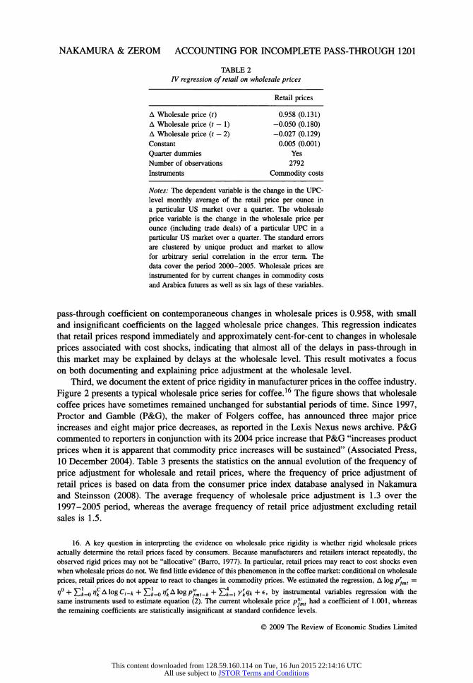
Third, we document the extent of price rigidity in manufacturer prices in the coffee industry. Figure 2 presents a typical wholesale price series for coffee.16 The figure shows that wholesale coffee prices have sometimes remained unchanged for substantial periods of time. Since 1997, Proctor and Gamble (P&G), the maker of Folgers coffee, has announced three major price increases and eight major price decreases, as reported in the Lexis Nexus news archive. P&G commented to reporters in conjunction with its 2004 price increase that P&G "increases product prices when it is apparent that commodity price increases will be sustained" (Associated Press, 10 December 2004). Table 3 presents the statistics on the annual evolution of the frequency of price adjustment for wholesale and retail prices, where the frequency of price adjustment of retail prices is based on data from the consumer price index database analysed in Nakamura and Steinsson (2008). The average frequency of wholesale price adjustment is 1.3 over the 1997-2005 period, whereas the average frequency of retail price adjustment excluding retail sales is 1.5.
16. A key question in interpreting the evidence on wholesale price rigidity is whether rigid wholesale prices actually determine the retail prices faced by consumers. Because manufacturers and retailers interact repeatedly, the observed rigid prices may not be "allocative" (Barro, 1977). In particular, retail prices may react to cost shocks even when wholesale prices do not. We find little evidence of this phenomenon in the coffee market: conditional on wholesale prices, retail prices do not appear to react to changes in commodity prices. We estimated the regression, A log pr-mt =
r}° + Yjc=o ̂^ A log Ct-k + Yjc=o *?* A log pjmt_k + Ylt=i YkQk + e» by instrumental variables regression with the same instruments used to estimate equation (2). The current wholesale price pjmt had a coefficient of 1.001, whereas the remaining coefficients are statistically insignificant at standard confidence levels.
© 2009 The Review of Economic Studies Limited
This content downloaded from 128.59.160.114 on Tue, 16 Jun 2015 22:14:16 UTCAll use subject to JSTOR Terms and Conditions
1202 REVIEW OF ECONOMIC STUDIES
Figure 2 A typical wholesale price series
The wholesale price depicted is for a leading coffee brand. The coffee commodity index is the "composite commodity index" discussed in Section 2. The gap in the retail price series from November 1998 to September 1999 arises due to missing data.
TABLE 3 Annual frequency of price change
Retail prices
Wholesale prices Without retail sales With retail sales
1.3 1.5 3.1
Notes: The wholesale price statistics are based on weekly wholesale price data for the period 1997-2004. The first column presents the statistics for regular prices (excluding trade deals). The observations are weighted by average retan revenue over the period 2000-2004. The second and third columns of present statistics on the frequency of price change for retail prices of ground coffee from Nakamura and Steinsson (2008) based on monthly data from the CPI research database collected by the Bureau of Labor Statistics.
There is a strong and statistically significant relationship between commodity cost volatility and the frequency of price change. Table 4 presents statistics on the average number of wholesale price adjustments per year over the period 1997-2003. Over the years 1997-2005, the average number of price changes in a year varied between 0.2 and 4.3 for wholesale price © 2009 The Review of Economic Studies Limited
This content downloaded from 128.59.160.114 on Tue, 16 Jun 2015 22:14:16 UTCAll use subject to JSTOR Terms and Conditions

NAKAMURA & ZEROM ACCOUNTING FOR INCOMPLETE PASS-THROUGH 1203
TABLE 4 Frequency of price change and commodity cost volatility
Average number of Standard deviation of Year price changes commodity cost index
1997 4.3 2.1 1998 1.7 1.6 1999 1.7 0.8 2000 3.0 0.9 2001 1.0 0.4 2002 0.4 0.3 2003 0.2 0.1 2004 0.6 0.5
Notes: The second column gives a size-weighted average of the annual frequency of wholesale price change, not including trade deals. These statistics are based on weekly wholesale price data for the period 1997-2004. The observations are weighted by average retail revenue over the period 2000-2004 (the period covered by the retail data). The third column gives the standard deviation of the coffee commodity index in units of cents per ounce.
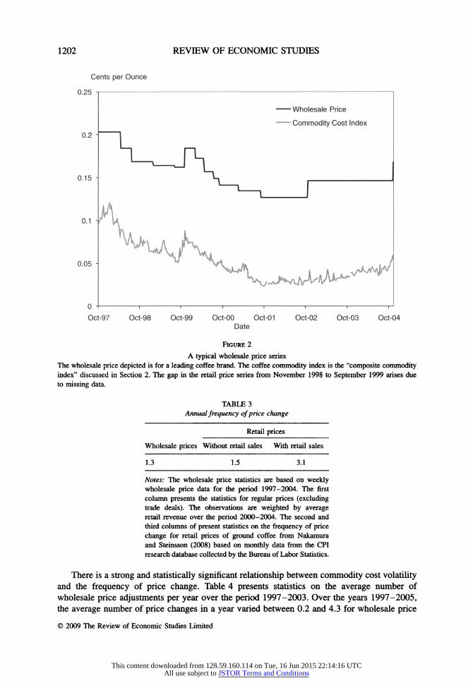
changes not including trade deals. Figure 3 plots the relationship between the average frequency of wholesale price changes and the annual volatility of the monthly commodity cost index for the years 1997-2005, illustrating a strong positive relationship.
4. CONSUMER DEMAND
The first building block of our structural model of the coffee industry is a model of con- sumer demand. We estimate a random coefficients discrete choice model for demand (Berry, Levinsohn and Pakes, 1995). 17 In this model, the consumer is assumed to select the product that yields the highest level of utility, where the indirect utility of individual i from purchasing product j takes the form,
Uijmt = <*? + afte- - prjmt) + Xjßx + Çjmt + €ijmti (3)
where af is the parameter governing the individual-specific price sensitivity of consumers, a® governs the individual-specific value of purchasing a product (set to zero if the outside option is chosen), y¿ is income, pr}mt is the price in market m at time t, Xj is a vector of product characteristics, ßx is a vector of parameters and £;mi is an unobserved demand shifter that varies across products and regions.18 We also allow the consumer to select the outside option of not purchasing ground caffeinated coffee. Because the mean utility from the outside option is not separately identified, we normalize it to zero. For computational tractability, the idiosyncratic error term €¡jmt is assumed to be distributed according to the extreme value dis- tribution. Demand, in ounces of coffee, is then given by the market share Sjmt9 the fraction of consumers for whom product j yields the highest value of utility, multiplied by the size of the market M .
17. Discrete choice models have been applied widely in the empirical organization literature. Other applications include shopping destination choice (McFadden, 1974), cereal (Nevo, 2001) and yogurt (Villas-Boas, 2007). See Anderson, Palma and Thisse (1992) for an overview of this class of models.
18. This expression for indirect utility may be derived from a quasi-linear utility function.
© 2009 The Review of Economic Studies Limited
This content downloaded from 128.59.160.114 on Tue, 16 Jun 2015 22:14:16 UTCAll use subject to JSTOR Terms and Conditions

1204 REVIEW OF ECONOMIC STUDIES
Annual Frequency
5.0 H «
4.0 -
3.0 - ♦
20 -
♦ ♦
1.0 - ♦
0.0 -I 1 1 , , 0.000 0.005 0.010 0.015 0.020 0.025
Volatility
Figure 3 Price change frequency versus commodity cost volatility
The figure plots the revenue-weighted average annual frequency of price change for the wholesale price (not including trade deals) vs. the volatility of the commodity cost index for each of the years 1997-2004. The revenue weights are constructed from average retail revenue over the period 2000-2004.
The key advantage of this type of structural model relative to an unrestricted model of demand is that it allows for a substantial reduction in the number of parameters that must be estimated, while still allowing for a substantial amount of flexibility in substitution patterns. To build intuition, we begin by estimating the logit model, a simplified version of the full model in which af = ap and or? = a0 for all i. In this case, the model implies the following equation for aggregate shares,
logsjmt - log s0 = a° - apprjmt + Xjß + Çjmt, (4)
where «o is a constant. We estimate the model on monthly price and market share data for ground, caffeinated coffee for 50 US markets as defined by AC Nielsen, where the prices and market shares are averages by market, brand, time period and size.19
The market for ground coffee is highly concentrated. To give a feel for the market structure of the coffee industry, let us note that the largest coffee manufacturers in the United States are Folgers and Maxwell House, which are owned by Proctor & Gamble and Kraft Foods,
19. Many retailers do not stock multiple UPCs within a brand-size category, suggesting that this may be a more appropriate specification than one based on individual UPCs.
© 2009 The Review of Economic Studies Limited
This content downloaded from 128.59.160.114 on Tue, 16 Jun 2015 22:14:16 UTCAll use subject to JSTOR Terms and Conditions

NAKAMURA & ZEROM ACCOUNTING FOR INCOMPLETE PASS-THROUGH 1205
respectively. Across markets, the median Herfindahl index is 0.35 and the median fraction of coffee sales accounted for by Proctor & Gamble and Kraft alone is 0.80. Folgers and Maxwell House have substantial market shares in all of the markets considered in this study and have national market shares by volume of roughly 38% and 32%, respectively, as a fraction of all caffeinated ground coffee sales. Geographically, Folgers is more popular in the West Coast and Midwestern US markets, whereas Maxwell House is more popular in Northeastern US markets. The third largest coffee manufacturer is Sara Lee, which has a national market share of roughly 7%. Sara Lee manufactures several smaller brands, including Hills Bros., Chock Full O' Nuts and MJB, which each have 2-4% of national market share by vol- ume but are only available in 40-50% of the markets we study. Two other important brands are Yuban (also produced by Proctor & Gamble) and Starbucks, which each have a mar- ket share by volume of 2-3%. The remaining brands in our sample are smaller regional brands whose sales are mainly limited to a handful of regionally concentrated markets. Among consumer packaged goods, store brands account for a relatively small fraction of total sales (4.7%).
The model is estimated using the top 15 products by volume sold nationally over the 5-year sample period of 2000-2004.20 These products account for 87% of the total AC Nielsen caffeinated ground coffee sales over this period. To estimate the demand system, it is necessary to define the total potential market M . We define the relevant market as two cups of caffeinated coffee (made from ground coffee purchased at supermarkets) for every individual 18 or over in a given market area per day.21
The classic econometric problem in demand estimation is the endogeneity of prices. Firms are likely to set high prices for products with high values of the omitted characteristic £;mi. This will bias price elasticity estimates towards zero. Intuitively, the price elasticities are biased downward because the model does not account for the fact that high-priced products are also likely to be particularly desirable. The first column of Table 5 (OLS1) presents estimates of equation (4) where Xj includes only advertising, a dummy for product size, dummy variables for years, as well as a dummy variable for December to account for demand fluctuations asso- ciated with Christmas. The advertising data are brand-level monthly national total advertising dollars per brand from the AdDollars database. Standard errors are clustered by unique product and market to allow for unrestricted time series correlation in the error term. This specification yields an inelastic demand curve for the majority of products and time periods: the median price elasticity is 0.54.
The panel structure of the data implies that we can account for fixed differences in £;mi in a flexible manner by introducing dummy variables (Nevo, 2001). These dummy variables allow for constant differences in utility across products, as well as regional differences in the mean utility of products. The second column of Table 5 (OLS2) presents estimates for the logit
20. Specifically, we include the following products in our estimation (market shares by volume in parentheses): Cafe Bustelo (0.8%), Chock Full 'O Nuts large (1.3%) and small (2.9%), Community (1.7%), Don Francisco's (1.0%), Folgers large (27.1%) and small (11.1%), Hills Bros large (2.6%), Maxwell House large (19.6%) and small (12.0%), MJB large (1.1%), Savarin (0.7%), Starbucks (1.7%), Yuban large (2.1%) and small (1.0%), where the product size is small unless otherwise indicated. Folgers and Maxwell House appear in nearly every market, and Hills Bros., Chock Full O' Nuts, MJB, Yuban and Starbucks appear in a large fraction (40-70% of markets), whereas the remaining brands appear in only a small number of markets. This yields a median of seven products and five brands per market.
21. The adult population in a market area is determined by multiplying the total population in a given area (provided by AC Nielsen) by the fraction of adults in a given area, calculated using the Current Population Survey. This specification implies that, depending on the market and time period, the market share of the outside option is between 21% and 89% with a median value of 74%.
© 2009 The Review of Economic Studies Limited
This content downloaded from 128.59.160.114 on Tue, 16 Jun 2015 22:14:16 UTCAll use subject to JSTOR Terms and Conditions
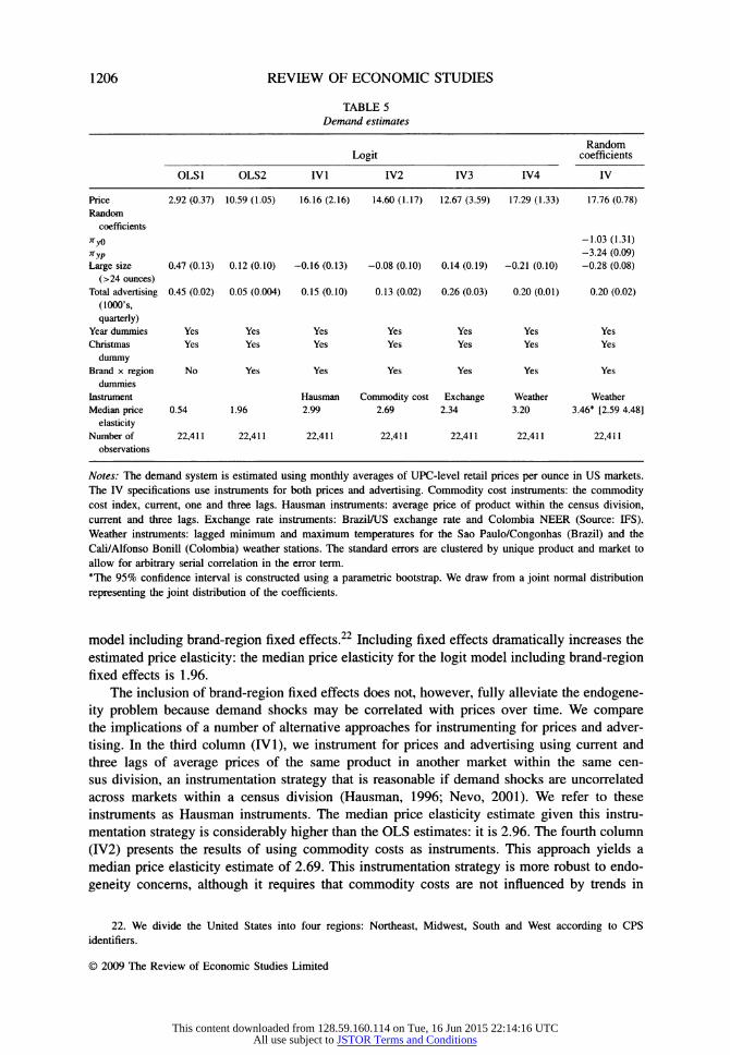
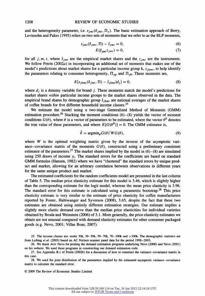
1206 REVIEW OF ECONOMIC STUDIES
TABLE 5 Demand estimates
Random Logit coefficients
OLS1 OLS2 IVI IV2 IV3 IV4 IV
Price 2.92(0.37) 10.59(1.05) 16.16(2.16) 14.60(1.17) 12.67(3.59) 17.29(1.33) 17.76(0.78) Random
coefficients
XyO -1.03(1.31) Ttyp -3.24 (0.09) Large size 0.47(0.13) 0.12(0.10) -0.16(0.13) -0.08(0.10) 0.14(0.19) -0.21(0.10) -0.28(0.08)
(>24 ounces) Total advertising 0.45(0.02) 0.05(0.004) 0.15(0.10) 0.13(0.02) 0.26(0.03) 0.20(0.01) 0.20(0.02)
(1000's, quarterly)
Year dummies Yes Yes Yes Yes Yes Yes Yes Christmas Yes Yes Yes Yes Yes Yes Yes
dummy Brand x region No Yes Yes Yes Yes Yes Yes
dummies Instrument Hausman Commodity cost Exchange Weather Weather Median price 0.54 1.96 2.99 2.69 2.34 3.20 3.46* [2.59 4.48]
elasticity Number of 22,411 22,411 22,411 22,411 22,411 22,411 22,411
observations
Notes: The demand system is estimated using monthly averages of UPC-level retail prices per ounce in US markets. The IV specifications use instruments for both prices and advertising. Commodity cost instruments: the commodity cost index, current, one and three lags. Hausman instruments: average price of product within the census division, current and three lags. Exchange rate instruments: Brazil/US exchange rate and Colombia NEER (Source: IFS). Weather instruments: lagged minimum and maximum temperatures for the Sao Paulo/Congonhas (Brazil) and the Cali/Alfonso Bonill (Colombia) weather stations. The standard errors are clustered by unique product and market to allow for arbitrary serial correlation in the error term. *The 95% confidence interval is constructed using a parametric bootstrap. We draw from a joint normal distribution
representing the joint distribution of the coefficients.
model including brand-region fixed effects.22 Including fixed effects dramatically increases the estimated price elasticity: the median price elasticity for the logit model including brand-region fixed effects is 1.96.
The inclusion of brand-region fixed effects does not, however, fully alleviate the endogene- ity problem because demand shocks may be correlated with prices over time. We compare the implications of a number of alternative approaches for instrumenting for prices and adver- tising. In the third column (IVI), we instrument for prices and advertising using current and three lags of average prices of the same product in another market within the same cen- sus division, an instrumentation strategy that is reasonable if demand shocks are uncorrelated across markets within a census division (Hausman, 1996; Nevo, 2001). We refer to these instruments as Hausman instruments. The median price elasticity estimate given this instru- mentation strategy is considerably higher than the OLS estimates: it is 2.96. The fourth column (IV2) presents the results of using commodity costs as instruments. This approach yields a median price elasticity estimate of 2.69. This instrumentation strategy is more robust to endo- geneity concerns, although it requires that commodity costs are not influenced by trends in
22. We divide the United States into four regions: Northeast, Midwest, South and West according to CPS identifiers.
© 2009 The Review of Economic Studies Limited
This content downloaded from 128.59.160.114 on Tue, 16 Jun 2015 22:14:16 UTCAll use subject to JSTOR Terms and Conditions

NAKAMURA & ZEROM ACCOUNTING FOR INCOMPLETE PASS-THROUGH 1207
demand for coffee in the US market. The fifth column (IV3) presents results using the Brazil- ian and Colombian exchange rates as instruments. This yields a slightly lower price elasticity of 2.34.
The sixth column (IV4) presents the results from using weather instruments: lagged mini- mum and maximum temperatures for the Sao Paulo-Congonhas (Brazil) and the Cali-Alfonso Bonill (Colombia) weather stations as instruments. We chose these weather stations because Colombia and Brazil are two of the largest exporters of green bean coffee and because they are located at high elevations where coffee is typically grown. The weather instruments have an R2 of 23% in explaining average monthly retail prices (27% for non-sale retail prices) and 13% in explaining average monthly advertising expenditures, once the series are adjusted for a year trend and a dummy for Christmas. This approach yields a price elasticity of 3.2. Because the weather instruments have the advantage that they are least likely to be plagued by endogeneity concerns, we focus on this instrumentation strategy in the random coefficients estimates below.23
A disadvantage of the logit model noted by many authors is that it implies unrealistic substitution patterns. For example, as the price of a "premium" product increases, there is no tendency for demand to shift to other premium products rather than to other less similar prod- ucts. One way of generalizing the model is to allow for heterogeneity in individual preferences (Berry, Levinsohn and Pakes, 1995). In our baseline results, we estimate a simple version of the random coefficients model, equation (3), in which an individual's price sensitivity as well as the mean utility of purchasing coffee is allowed to vary with his or her household income.
<*,-=« + n^/, (5)
where a¡ = [off, af ]', a = [a0, ap]' U = [fl^o, n^]' and y¡ is household income normalized, for ease of interpretation, to have mean zero and variance of one across all markets that we consider. We assume that y¡ has a log-normal distribution within markets, where the parameters of this distribution are chosen to match the observed distribution of household income within each market for individuals over 18 in the March Supplement of the 2000 CPS after trimming the bottom 2.5% of the sample (which includes negative and zero income observations). This model allows for both heterogeneity in income within individual markets and variation in the mean and variance of the income distribution across markets.
A negative value for Ylyp indicates that higher income consumers are less responsive to prices. This parameter has important implications for the curvature of demand: if there is a substantial amount of heterogeneity in price sensitivity across consumers (Ylyp is large in absolute value), then as a firm raises its price, its consumer base is increasingly dominated by households with low price sensitivities, lowering the price elasticity faced by the firm.
Let us now describe our estimation procedure for our full demand model. It will be useful in describing the procedure to rewrite the indirect utility as £/iymi = Sjmt + Pijmt + €Umt where Sjmt captures the component of utility common to all consumers and /¿¿ym, is a mean- zero heteroskedastic term that reflects individual deviations from this mean.24 Given this decomposition, the aggregate market shares may be written as a function of the mean utility
23. A second econometric concern is whether the rank condition for IV estimation is satisfied. Our analysis of this issue (see the working paper version of this paper) indicates that the rank condition is likely to be satisfied. We thank an anonymous referee for encouraging us to study the rank condition, and Serena Ng for advice on how to
analyse this issue. 24. In particular, the mean utility and individual component are given by Sjmt = or - ap prjmt +*jßx + H jmt
and pijmt = Uyoyi - nypyiprjmr
© 2009 The Review of Economic Studies Limited
This content downloaded from 128.59.160.114 on Tue, 16 Jun 2015 22:14:16 UTCAll use subject to JSTOR Terms and Conditions
1208 REVIEW OF ECONOMIC STUDIES
and the heterogeneity parameter, i.e. Sjmt(8jmti Yly). The basic estimation approach of Berry, Levinsohn and Pakes (1995) relies on two sets of moments that we refer to as the BLP moments,
Sjmt (Sjmt, n) - Sjmt = 0, (6)
EiHjmtZjmt) = 0, (7)
for all y, m, t, where Sjmt are the empirical market shares and the Zjmt are the instruments. We follow Pétrin (2002a) in incorporating an additional set of moments that makes use of the model's predictions about market shares for a particular income group k, Sjkmt, to help identify the parameters relating to consumer heterogeneity, Y'yp and n^o- These moments are,
E[sjkmt(8jmt, n) - SjtmtWj] = 0, (8)
where dj is a dummy variable for brand j. These moments match the model's predictions for market shares within particular income groups to the market shares observed in the data. The empirical brand shares by demographic group Sjkmt are national averages of the market shares of coffee brands for five different household income classes.25
We estimate the model using a two-stage Generalized Method of Moments (GMM) estimation procedure.26 Stacking the moment conditions (6) -(8) yields the vector of moment conditions G(0), where 0 is a vector of parameters to be estimated, where the vector 0° denotes the true value of these parameters, and where E[G(00)] = 0. The GMM estimator is,
0 = aigmineG(0yWG(0), (9)
where W is the optimal weighting matrix given by the inverse of the asymptotic vari- ance-covariance matrix of the moments G(0), constructed using a preliminary consistent estimator of the parameters.27 The market shares implied by the model in (6)-(8) are simulated using 250 draws of income y¡. The standard errors for the coefficients are based on standard GMM formulas (Hansen, 1982) where we have "clustered" the standard errors by unique prod- uct and market, allowing for an arbitrary correlation between observations in different years for the same unique product and market.
The estimated coefficients for the random coefficients model are presented in the last column of Table 5. The median price elasticity estimate for this model is 3.46, which is slightly higher than the corresponding estimate for the logit model, whereas the mean price elasticity is 3.96. The standard error for this estimate is calculated using a parametric bootstrap.28 This price elasticity estimate is very similar to the estimate of price elasticity for coffee manufacturers reported by Foster, Haltiwanger and Syverson (2008), 3.65, despite the fact that these two estimates are obtained using entirely different estimation strategies. Our estimate implies a slightly more elastic demand curve than the median price elasticities for individual varieties obtained by Broda and Weinstein (2006) of 3.1. More generally, the price elasticity estimates we obtain are not unusual compared with demand elasticity estimates for other consumer packaged goods (e.g. Nevo, 2001; Villas Boas, 2007).
25. The income classes are: under 30k, 30-50k, 50-70k, 70- 100k and >100k. The demographic statistics are from Leibtag et al (2005) based on AC Nielsen scanner panel data for the period 1998-2003.
26. We thank Aviv Nevo for posting the demand estimation programs underlying Nevo (2000) and Nevo (2001) on his website. We used these programs in constructing our demand estimation code.
27. See Appendix B.I of Pétrin (2002£) for a discussion of how to construct the variance-covariance matrix in this case.
28. We used the joint distribution of the parameters implied by the estimated asymptotic variance-covariance matrix to calculate the standard error.
© 2009 The Review of Economic Studies Limited
This content downloaded from 128.59.160.114 on Tue, 16 Jun 2015 22:14:16 UTCAll use subject to JSTOR Terms and Conditions
NAKAMURA & ZEROM ACCOUNTING FOR INCOMPLETE PASS-THROUGH 1209
We estimate a moderate degree of heterogeneity in the price elasticity parameter. The estimated value of Uyp is -3.24, indicating that high-income households have moderately lower price elasticities than low-income consumers. A household with an income one standard deviation above the mean has a price elasticity about 20% below the price elasticity of the median consumer. The income heterogeneity parameter nyp plays an important role in determining pass-through because it governs how the price elasticity faced by a firm changes as the firm raises its prices. The point estimate of heterogeneity in the mean utility of coffee Ilyo is negative (-1.03), indicating that higher income consumers have a slightly lower utility for ground coffee, as opposed to not purchasing coffee at all, or purchasing pre-made coffee at a cafe. However, this parameter is not statistically significantly different from zero at standard confidence levels.
A key determinant of the response of prices to changes in costs is the "super-elasticity" of demand - the percentage change in the price elasticity for a given percentage increase in prices (Klenow and Willis, 2006). The super-elasticity is a quantitative measure of the curvature of demand. The workhorse Dixit-Stiglitz demand model has a super-elasticity of zero, implying a constant markup under monopolistic competition. A positive super-elasticity of demand implies that as a firm raises its price, the price elasticity it faces increases. We estimate the super-elasticity of demand to be 4.64 in the random coefficients model. In other words, a 1% increase in prices leads to a 4.64% increase in the price elasticity of demand. This generates a substantial motive for the firm to adjust its markup.
Because the demand curve is an important input into our empirical exercise, we also carried out a number of robustness exercises. In addition to our baseline random coefficients demand model, we also estimated a specification that allows for an additional degree of heterogeneity in consumer preferences that is unrelated to income,
a¡ =a + ri5?/ + nvv/, (10)
where v, is distributed normally with mean zero and variance one. Because this specification is difficult to identify using only time series variation in prices, we estimated the model using both the weather instruments and the Hausman instruments described above. The Hausman instru- ments have the advantage that they vary across different products, as well as over time. This specification yields estimates of n^ = -3.41, F^o = -0.92 and ny = 2.76, with an implied median price elasticity of 3.63 and a super-elasticity of 4.81. As an additional robustness check, we also re-estimated our baseline specification of the random coefficients model using only the BLP moment conditions, equations (6) and (7), using the original weather instruments. Although this approach yields much less precise estimates, it has the advantage that it relies less on the structure of the model, because in this case, the curvature of the demand curve is estimated purely based on time series variation in prices and costs. Again, this estimation approach yields similar point estimates of the key parameters to the baseline approach. This estimation approach yields a median price elasticity of 3.96 and a median price super-elasticity of 4.37.
5. LOCAL COSTS
In modelling the response of prices to costs in the coffee industry, an important consid- eration is that only some fraction of marginal costs are accounted for by coffee beans. The remaining "local costs" of production play an important role in determining pass- through behaviour because they drive a wedge between fluctuations in imported costs and the marginal cost of production (Sanyal and Jones, 1982; Burstein, Neves and Rebelo, 2003;
© 2009 The Review of Economic Studies Limited
This content downloaded from 128.59.160.114 on Tue, 16 Jun 2015 22:14:16 UTCAll use subject to JSTOR Terms and Conditions
1210 REVIEW OF ECONOMIC STUDIES
Corsetti and Dedola, 2005). If local costs are large, even a substantial increase in the price of an imported factor of production may increase total marginal costs by only a small fraction.
The magnitude of the local costs cannot be observed directly. The oligopolistic structure of the market implies that the difference between prices and commodity costs reflects a combination of marginal costs and oligopolistic markups. Given a particular model of the supply side of the industry, it is possible to infer the markup by "inverting" the demand system to find the vector of marginal costs that rationalizes firms' observed pricing behaviour. Because we know exactly how many ounces of green bean coffee are used to produce a given quantity of ground coffee, we can then obtain estimates of the local costs of production by subtracting commodity costs from the inferred marginal costs.29
We will ultimately be interested in a dynamic model of pricing that allows for price rigidity. We begin, however, by inferring markups for a static Nash-Bertrand equilibrium (Bresnahan, 1987; Berry, Levinsohn and Pakes, 1995). To avoid searching over a large parameter space as part of the dynamic estimation procedure, we use the estimates of local costs from the static model in the baseline parameterization of the dynamic model analysed in Section 6. This procedure is exactly correct if the introduction of menu costs only affects the dynamic response of prices to costs but does not affect the level of prices. Although this holds exactly in some simple models (e.g. Dixit, 1991), it does not hold exactly in our model due to asymmetries in the profit function and strategic interactions. In Section 6, we consider an alternative procedure in which we estimate a common component of local costs as part of the dynamic estimation procedure, which yields very similar results.
Let us begin by describing the static model. The supply side of the model consists of J multi-product firms that each produce some subset of the products. We fix the number of firms and the products produced by the firms to match the observed industry structure (e.g. the mar- ket share of Folgers and Maxwell House). Firm j's per-period profits n jmt in a market m at time t may be written,
71 jmt = Yl (pkmt - mCkmt)Mskmt - Fkm, (11) keTj
where mckmt is the marginal cost of producing the product, F*m is a fixed cost, Ty is the set of products produced by firm j and M is the size of the market. We assume a reduced form model of retailer behaviour: retail prices prkmt depend on wholesale prices such that ^Pr^PÌkmty^PÌcmt = 1- This assumption is consistent with the empirical response of retail prices to wholesale price changes documented in Section 3.30
We assume that firms set wholesale prices to maximize the profits associated with their products in a Bertrand-Nash fashion. In all of the analysis that follows, we assume that the coffee manufacturers take marginal costs as given. The optimizing firms' prices satisfy the first-order conditions,
. V^ / w ' "Skint ~ /ir»' Skmt +
. V^ > (Pkmt
/ w - mCkm,)--- ' = 0.
~ (12) /ir»'
29. The simple (and known) production relationship between green bean coffee and ground coffee is an advantage of studying the coffee market. In other markets it is necessary to estimate a production function to determine the contribution of imported inputs to production costs (see, for example, Goldberg and Verbo ven' s (2001) analysis of the auto industry).
30. This assumption could be micro-founded, for example, by assuming that retailers face demand given by a logit demand model.
© 2009 The Review of Economic Studies Limited
This content downloaded from 128.59.160.114 on Tue, 16 Jun 2015 22:14:16 UTCAll use subject to JSTOR Terms and Conditions
NAKAMURA & ZEROM ACCOUNTING FOR INCOMPLETE PASS-THROUGH 121 1
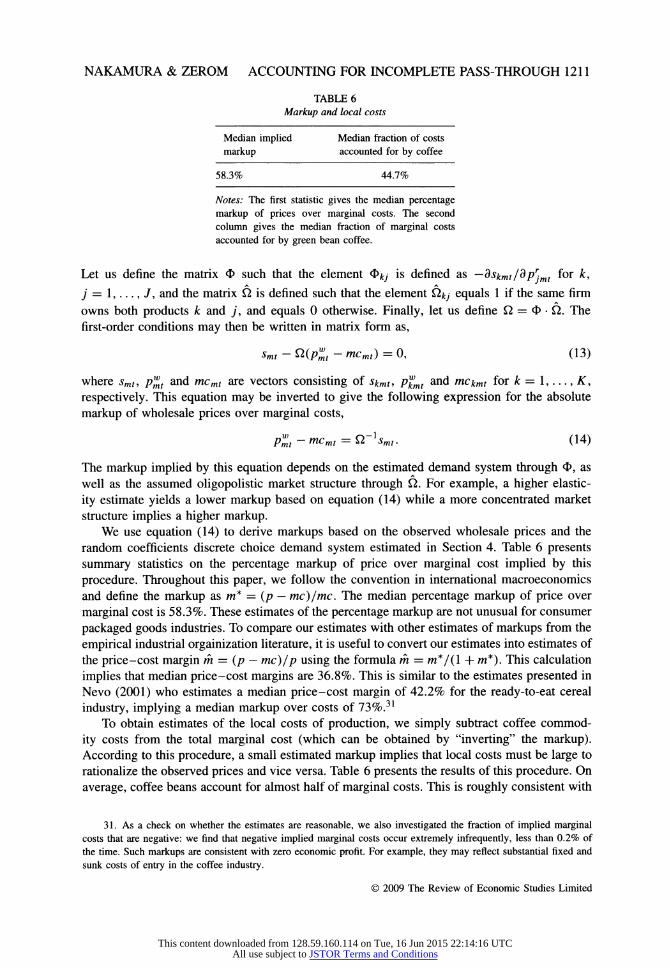
TABLE 6 Markup and local costs
Median implied Median fraction of costs markup accounted for by coffee
58.3% 44.7%
Notes: The first statistic gives the median percentage markup of prices over marginal costs. The second column gives the median fraction of marginal costs accounted for by green bean coffee.
Let us define the matrix O such that the element O*; is defined as -dskmt/dprjmt for &» j = 1, . . . , J, and the matrix Û is defined such that the element Ûy equals 1 if the same firm owns both products k and j, and equals 0 otherwise. Finally, let us define Q = O • Ù. The first-order conditions may then be written in matrix form as,
smt - Q(p2 - mcmt) = 0, (13)
where smt, p%t and mcmt are vectors consisting of Skmi, p™mt and mckmt for fc = 1, . . . , AT, respectively. This equation may be inverted to give the following expression for the absolute markup of wholesale prices over marginal costs,
pZ-mcmt = Q-lsmt. (14)
The markup implied by this equation depends on the estimated demand system through 4>, as well as the assumed oligopolistic market structure through Ù. For example, a higher elastic- ity estimate yields a lower markup based on equation (14) while a more concentrated market structure implies a higher markup.
We use equation (14) to derive markups based on the observed wholesale prices and the random coefficients discrete choice demand system estimated in Section 4. Table 6 presents summary statistics on the percentage markup of price over marginal cost implied by this procedure. Throughout this paper, we follow the convention in international macroeconomics and define the markup as m* = (p - me) /me. The median percentage markup of price over marginal cost is 58.3%. These estimates of the percentage markup are not unusual for consumer packaged goods industries. To compare our estimates with other estimates of markups from the empirical industrial orgainization literature, it is useful to convert our estimates into estimates of the price-cost margin m = (p - mc)/p using the formula m = m* /(I + m*). This calculation implies that median price-cost margins are 36.8%. This is similar to the estimates presented in Nevo (2001) who estimates a median price-cost margin of 42.2% for the ready-to-eat cereal industry, implying a median markup over costs of 73 %.31
To obtain estimates of the local costs of production, we simply subtract coffee commod- ity costs from the total marginal cost (which can be obtained by "inverting" the markup). According to this procedure, a small estimated markup implies that local costs must be large to rationalize the observed prices and vice versa. Table 6 presents the results of this procedure. On average, coffee beans account for almost half of marginal costs. This is roughly consistent with
31. As a check on whether the estimates are reasonable, we also investigated the fraction of implied marginal costs that are negative: we find that negative implied marginal costs occur extremely infrequently, less than 0.2% of the time. Such markups are consistent with zero economic profit. For example, they may reflect substantial fixed and sunk costs of entry in the coffee industry.
© 2009 The Review of Economic Studies Limited
This content downloaded from 128.59.160.114 on Tue, 16 Jun 2015 22:14:16 UTCAll use subject to JSTOR Terms and Conditions
1212 REVIEW OF ECONOMIC STUDIES
industry estimates of the magnitude of non-coffee costs reported in Yip and Williams (1985), estimates based on the Survey of Manufacturers, and Bettendorf and Verbo ven' s (2000) results for the Dutch coffee market.
6. A MENU COST MODEL OF AN OLIGOPOLY
The standard static pricing model discussed in the previous section does not account for the infrequent price adjustments or delayed price responses documented in Section 3. In this section, we therefore extend the model to allow for adjustment costs in price-setting. This introduces dynamic considerations: if a cost change is expected to persist for many periods, a forward-looking firm may choose to adjust its prices even if the current benefit from doing so is quite small. Furthermore, given the oligopoly setting, prices become a strategic variable that may influence the pricing decisions of a firm's competitors.
The model builds on previous menu cost models estimated using dynamic methods by Slade (1998, 1999) and Aguirregabiria (1999). The model we use is, however, somewhat different from these models in that we allow for random costs of adjustment. Although the distribution of these costs is known, the realization of the menu cost is private information. This model is formally related to the dynamic oligopoly model studied by Pakes and McGuire (1994).32 It is not possible to solve analytically for the Markov perfect equilibrium of the model. Therefore, we adopt methods from this literature (e.g. Benkard, 2004) to numerically solve for the equilibrium pricing policies of the firms. The equilibrium concept that we adopt is a Markov perfect Nash equilibrium, where the strategy space consists of firms' prices (Maskin and Tiróle, 1988). This equilibrium concept restricts attention to pay-off relevant state variables, thus focusing attention away from the large number of other sub-game perfect equilibria that exist in this type of model.
We use value function iteration to solve for the policies of the individual firms and then use an iterative algorithm to update the firms' policy functions until a fixed point is achieved. We assume that demand is given by the demand system estimated in Section 4. As in the case of the Pakes-McGuire algorithm, there is no guarantee that this algorithm converges.33
6.1. Model
The model consists of a small number of oligopolistic firms. Firm j seeks to maximize the discounted expected sum of future profits,
oo
£o £>' [njmtipl, C,) - YjmlHApJmt ¥> 0)] , (15)
where p%t is the vector of wholesale prices (per ounce) in market m at time t, 7tjmt is the firm's per-period profit, Ct is the commodity cost, ß is the firm's discount factor, y¡mt is a random
32. As in the dynamic oligopoly literature, the assumptions that the adjustment cost is random and that it is private information are helpful from a computational perspective because it implies that firms choose their actions in response to the expected policies of their competitors, which helps to smooth their responses. See Doraszelski and Pakes (2006) for a detailed overview of dynamic oligopoly models.
33. We are not aware of theoretical work guaranteeing the existence or uniqueness of a pure strategy equilibrium in this type of oligopoly model. Indeed, there is no proof of uniqueness even for the static oligopoly model with demand given by the discrete choice random coefficients model. We dealt with this issue by doing a numerical search for other equilibria by starting the computational algorithm at alternative initial values. This approach always yielded a unique equilibrium.
© 2009 The Review of Economic Studies Limited
This content downloaded from 128.59.160.114 on Tue, 16 Jun 2015 22:14:16 UTCAll use subject to JSTOR Terms and Conditions

NAKAMURA & ZEROM ACCOUNTING FOR INCOMPLETE PASS-THROUGH 1213
menu cost the firm pays if it changes its prices, and l(ApJmt ̂ 0) is an indicator function that equals one when the firm changes its price.34 Each firm maximizes profits. We assume that ß = 0.99. The firm's profits 7Tjmt(p%r Ct) are given by expression (11) above, where the relationship between retail and wholesale prices is discussed below. The firm's profits depend both on its own prices and the prices of its competitors through this profit function.35
The menu cost Yjmt is independent and identically distributed with an exponential distribution; i.e. F (Yjmt) = 1 - exp (-^Yjmt)- The firm's draw of the menu cost Yjmt is private information. In every period, the pricing game has the following structure:
1. Firms observe the commodity cost Ct and their own draws of the menu cost Yjmt- 2. Firms choose wholesale prices pjmt simultaneously (without observing other firm's draws
Of Yjmt)' The Bellman equation for firm y's dynamic pricing problem is thus,
Vj(Pm-l>Ct>Yjm,) = max E, [njmt{plt, Ct) - y,m( 1 ( A/,Jm, # 0) + W/C C,+1, yjmt+1)] , (16)
Pjmt
where Et is the expectation conditional on all information known by firm j at time t including its own menu cost Yjmt- The expectation is taken over two sources of uncertainty: uncertainty about the future commodity cost Ci+i and uncertainty about competitors' prices arising because the menu costs are private information. Notice that a given firm's profits and value function depend on all firms' prices through the demand curve. From the perspective of a firm's competitors, its strategy has two parts. First, the pricing rule ̂ (¿_i,G) for all firms j = 1, . . . , B gives the firm's price if it decides to change its price. Second, the probability function Vxj(Pm't-v ^t) gives the probability that the firm changes its price for a particular value of the publicly observable variables (p%t_i> Ct).
An equilibrium is defined as a situation where a firm chooses optimal policies (i.e. the Bellman equation (16) is satisfied), and the firm's expectations are consistent with the equilibrium behaviour of the firm's competitors. As we note above, the firm's strategy is restricted to be Markov; i.e. to depend only on the payoff-relevant state.
To make the problem computationally tractable, we make the following simplifying assumptions. First, we assume that the prices for different sizes of the same brand move together (i.e. if the per-ounce price of Folgers 16 ounce coffee increases by 10 cents then the same thing happens to the per-ounce price of Folgers 40 ounce coffee). Hence, we have,
Pbnt = P7ntí+«k, (17)
for all k eTj, where a¿ is a known parameter. This assumption is motivated by the fact that empirically, the timing of price changes is often coordinated across products owned by the same brand.36
34. Notice that this equation assumes that, although each firm produces multiple products, its pricing decisions across products are coordinated. We discuss this assumption below.
35. Notice that the demand shifter £ymi, discussed in Section 4, is assumed to be fixed at its product and market- specific mean. This is motivated by the fact that, in simulations of the static pricing model, time series variation in t-jmt explains very little of the observed variation of prices. This simplification substantially reduces the computational burden of solving and estimating the model since a full analysis of dynamic demand shocks would require several additional state variables.
36. Conditional on at least one product from a particular brand adjusting in a given month, the probability of adjustment across all products is 93.8% over the 1997-2005 period.
© 2009 The Review of Economic Studies Limited
This content downloaded from 128.59.160.114 on Tue, 16 Jun 2015 22:14:16 UTCAll use subject to JSTOR Terms and Conditions

1214 REVIEW OF ECONOMIC STUDIES
Second, we assume that retail prices equal wholesale prices plus a known constant mar- gin £t,
PL,=Sk + Phnr (18)
Marginal cost is modelled as the sum of a product-specific constant ¡ik and the commodity cost,
mckmt = iik + Ct. (19)
This specification is meant to capture the idea that non-coffee costs are several times less variable than coffee commodity costs. This specification also implies that marginal costs do not depend on the scale of production.
Uncertainty about future costs takes the form,
Ct =ao + PcCt-i+€c, (20)
where €c is distributed Af(O, o2c) and o2c, ao and pc are known coefficients. Because a unit root in commodity costs cannot be rejected at standard confidence levels, we model commodity costs as a random walk; i.e. ao = 0 and pc = 1. Firms' perceptions about the stochastic process of costs play a key role in determining pass-through, as we discuss in Section 7. For computational reasons, we assume that commodity costs follow a random walk so long as costs lie between the bounds CH and CL, but are bounded within this region.
The firm's decision about whether to adjust its price depends on the difference between its payoffs when it adjusts and when it does not adjust,
AW = Wch-Wnch, (21)
where Wch is the discounted expected value of the firm if it adjusts its price and Wnch is the discounted expected value of the firm if it maintains a fixed price, based on the firm's expectations regarding its competitors' prices. (Recall that the menu costs of a firm's competitors are assumed to be private information.) Given the pricing policies of its competitors, the firm adjusts its price if the benefits of doing so outweigh the costs. The firm's pricing policy is given by the following policy rule,
„. _M«r-i * *W<yJml Pjm'~'p7:, „.
otherwise (22)
where the firm's price conditional on adjustment is given by,
pj*t = argmax Et [njm{pl„ Ct) + ßVjip^,, Ct+U yjmt+l)] . (23) Pjmt
In an equilibrium, all firms set their prices according to the decision rule implied by equations (22) and (23). Solving for the firms' optimal policy functions is complicated by the fact that the firms' incentives to adjust their prices depend, in turn, on the prices of the other firms.
We solve the model numerically using the computational algorithm described in the online appendix to this paper. The algorithm is conceptually straightforward but computationally intensive. We begin with some initial values of the firms' pricing policies. For a given firm, say Firm 1, we solve for the optimal dynamic pricing policy conditional on the initial pricing policies of its competitors by value function iteration. We use the solution to this problem to update the assumed pricing policy for Firm 1. Next, we solve for Firm 2' s optimal dynamic pricing policy, conditioning on the updated pricing policy for Firm 1. We repeat this exercise until the maximum differences in the firms' pricing policies between successive iterations are sufficiently small. Once this point is reached, we run our algorithm for an additional 1500 iterations to check that the equilibrium does not change.
© 2009 The Review of Economic Studies Limited
This content downloaded from 128.59.160.114 on Tue, 16 Jun 2015 22:14:16 UTCAll use subject to JSTOR Terms and Conditions
NAKAMURA & ZEROM ACCOUNTING FOR INCOMPLETE PASS-THROUGH 1215
6.2. Parameters
Given the computationally intensive nature of the iterative procedure, it is not possible to sep- arately analyse the implications for all possible markets. We focus on a representative market: the Syracuse market. The Syracuse market has a representative market structure dominated by P&G (Folgers), Kraft (Maxwell House) and Sara Lee (Hills Brothers). The average annual rev- enue in the Syracuse market is approximately 3 million dollars, which is close to the median across markets in the sample. Each brand produces two different products according to the definition discussed in Section 4, so we have two products per firm and six products in total.
We parameterize the demand curve according to the random coefficients discrete choice model estimated in Section 4. The demand curve also plays an important role in parameterizing local non-coffee costs. In our baseline specification of the dynamic model, we make use of the estimates of average non-coffee costs, ßkm, implied by the static pricing model described in Section 5. Specifically, we take fikm to be the average non-coffee costs,
i T
^km = jY. [Pkmt - V>-Xskmt - G] . (24) t='
Since these estimates are based on the static model they do not account for the role of menu costs. Menu costs could affect average equilibrium prices through strategic interactions and asymmetries in the profit function. This, in turn, could lead to different estimates of local costs. To gauge the robustness of the procedure used to estimate local costs, we also consider an alternative approach in which we estimate a common component of marginal costs as part of the dynamic estimation procedure in Appendix A. This procedure turns out to yield very similar results, since menu costs have little effect on average equilibrium prices.
We parameterize the retail margin %k as the average difference between retail and wholesale prices for a particular market and brand. Moreover, we parameterize the average price difference otk in equation (17) as the average observed difference in retail prices. We also condition on the observed value of wholesale prices in the period before the simulations begin (1999 Q4). We set the standard deviation of shocks to commodity costs equal to the observed standard deviation of commodity costs oq over the sample period.
The remaining parameter is the mean of the menu cost distribution, o . We estimate this parameter to match the observed frequency of wholesale price change using the indirect estimation approach of Gourieroux, Monfort and Renault (1993) for dynamic models. In particular, we use the following procedure in selecting the menu cost parameter. For different values of the menu cost parameter a, we simulate the model for the actual observed values of the commodity cost index over the 2000-2005 period. We then carry out a grid search over alternative possible values of or. The menu cost estimate is chosen to minimize the loss function,
L = (f- /)2. (25)
where / is the overall frequency of price change predicted by the model (across all time periods and brands), and / is the actual average frequency of price change excluding trade deals over the 2000-2005 period.37 The average frequency of price change excluding trade deals over this period was 1.3 times per year or a monthly frequency of about 11%. Figure 4 presents a
37. Gourieroux, Monfort and Renault (1993) do not formally extend their analysis to the case of dynamic models with discontinuities in the sample moment. However, Dridi (1999) argues that the technical apparatus used to analyse this case for static models may be extended to dynamic models. Magnac, Robin and Visser (1995) find that this estimator performs well in a dynamic model in Monte Carlo simulations.
© 2009 The Review of Economic Studies Limited
This content downloaded from 128.59.160.114 on Tue, 16 Jun 2015 22:14:16 UTCAll use subject to JSTOR Terms and Conditions
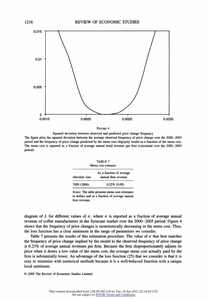
1216 REVIEW OF ECONOMIC STUDIES
0.015 "I V 1
0.01 ■ ' /
0.005 - ' /
0 H 1 -^ ^ 1
0.0015 0.0020 0.0025 0.0030
Figure 4
Squared deviation between observed and predicted price change frequency The figure plots the squared deviation between the average observed frequency of price change over the 2000-2005 period and the frequency of price change predicted by the menu cost oligopoly model as a function of the menu cost. The menu cost is reported as a fraction of average annual retail revenue per firm (calculated over the 2000-2005 period).
TABLE 7 Menu cost estimate
As a fraction of average Absolute size annual firm revenue
7000 (2806) 0.22% (0.09)
Notes: The table presents menu cost estimates in dollars and as a fraction of average annual firm revenue.
diagram of L for different values of a, where a is reported as a fraction of average annual revenue of coffee manufacturers in the Syracuse market over the 2000-2005 period. Figure 4 shows that the frequency of price changes is monotonically decreasing in the menu cost. Thus, the loss function has a clear minimum in the range of parameters we consider.
Table 7 presents the results of this estimation procedure. The value of a that best matches the frequency of price change implied by the model to the observed frequency of price change is 0.23% of average annual revenues per firm. Because the firm disproportionately adjusts its price when it draws a low value of the menu cost, the average menu cost actually paid by the firm is substantially lower. An advantage of the loss function (25) that we consider is that it is easy to minimize with numerical methods because it is a well-behaved function with a unique local minimum.
© 2009 The Review of Economic Studies Limited
This content downloaded from 128.59.160.114 on Tue, 16 Jun 2015 22:14:16 UTCAll use subject to JSTOR Terms and Conditions

NAKAMURA & ZEROM ACCOUNTING FOR INCOMPLETE PASS-THROUGH 1217
The standard error of this estimate may be calculated using the formulas presented in Gourieoux, Monfort and Renault (1993) for the case of static moments in dynamic models. In evaluating this formula, we use a numerical estimate of the derivative of the loss function with respect to the parameter estimate. We estimate the variance of the sample moment using a parametric bootstrap.38 This procedure yields a standard error of 0.09% for menu costs as a fraction of average annual revenues, implying an upper bound for the 95% confidence interval of the estimator of 0.33%.
There are few existing estimates of the costs of price adjustment at the manufacturer level. Zbaracki et al. (2004) estimate that costs of price adjustment account for 1.22% of annual revenue in a large industrial firm based on direct measures of the costs of price adjustment. Goldberg and Hellerstein (2007) estimate lower and upper bounds for menu costs in the beer industry of between 0 and 0.443% of revenue. Aguirregabiria (1999) and also Levy et al. (1997) estimate menu costs of 0.7% of revenue, although these estimates are less directly comparable with ours because they refer to retailer rather than manufacturer-level barriers to price adjustment. Slade (1998) estimates retail menu costs of $2.70 per price change for a particular retail store, but does not report the magnitude of the menu costs relative to annual revenues.
6.3. Equilibrium pricing policies
From the perspective of a firm's competitors, a firm's pricing policy gives (1) what price the firm adjusts to conditional on adjusting and (2) the probability of adjustment conditional on the publicly observable variables; i.e. p%t_x and Ct. Figure 5 plots an example (for a particular firm and time period) of a firm's probability of adjustment in period t as a function of its period t - 1 price. This figure gives the expected probability of adjustment, where the expectation is taken over different values of the random menu cost yjmt . In this example, the optimal dynamic price is $0.138 per ounce. At this price, the probability of adjustment is zero. The probability that the firm will adjust its price increases monotonically with the distance from the dynamic optimal price.
This pricing behaviour leads to delayed pass-through of costs into prices. The intuition is the following. In the first period after a shock, firms have a low probability of adjusting immediately in response to a change in costs. As shocks accumulate, however, the firm's probability of adjusting grows. Eventually, the firm adjusts to the new dynamic optimal price which reflects all of the cost shocks that have accumulated since its last price change.
A firm's optimal pricing policy also depends on its competitors' prices. The demand model described in Section 4 implies that prices may be either strategic complements or substitutes. For the estimated parameter values, prices are, in most (but not all) cases, strategic comple- ments. Figure 6 plots an example of Firm 3' s probability of adjustment as a function of its competitors' previous prices, all else constant. In this example, Firm 3' s dynamic optimal price lies above its price in the previous period. Because Firm 3' s price and its competitors' prices are strategic complements, Firm 3 has, for the most part, a higher probability of raising its price given higher values of its competitors' past prices. As Figure 6 shows, however, the probability of adjustment is not monotonically increasing in competitors' prices. Non-monotonic relation- ships of this nature arise frequently in this pricing game for the following reason. Firm 3 cares about the past prices of its competitors only through their potential effect on current prices. As
38. Specifically, we evaluate the sample moment for alternative draws of costs from the assumed Markov process for costs. We calculate the variance of the sample moment based on these draws. This approach takes into consideration sampling error in the menu cost as well as commodity costs, but not parameter uncertainty arising from the estimation of the demand system.
© 2009 The Review of Economic Studies Limited
This content downloaded from 128.59.160.114 on Tue, 16 Jun 2015 22:14:16 UTCAll use subject to JSTOR Terms and Conditions

1218 REVIEW OF ECONOMIC STUDIES
Probability 1 -
0.8 - N. ^S
0.6 - ' /
0.4 - ' /
0.2 - ' /
0-I i ^-*i 1
0.1 0.12 0.14 0.16
Initial Price
Figure 5
Probability of adjustment versus initial price This figure plots an example of the relationship between the probability of adjustment and the initial price in the menu cost oligopoly model.
a competitor's time t - 1 price rises, it becomes increasingly likely that the competitor will
readjust its price downward in period t, and this, in turn, lessens Firm 3' s incentive to raise its price.
7. DYNAMIC PRICING IMPLICATIONS
In this section, we analyse the implications of our model for short and long-run price dynamics. We begin by investigating whether the model can generate quantitatively realistic predictions for the timing of price adjustments, a key determinant of short-run price dynamics. To do this, we simulate the model for the actual sequence of costs over the 2000-2004 period based on the
equilibrium policy rules and the stochastic process generating costs, (20). For each simulation, we draw new values of the firms' menu costs. We then calculate the average frequency of price change by year across the simulations.
Figure 7 plots the annual frequency of price adjustment for the model versus the data. In the model, as in the data, the frequency of wholesale price change is strongly positively related to the volatility of commodity costs: the minimum average frequency of price adjustment in both the model and the data occurs in 2003, whereas the maximum occurs in 2000. The model is also able to explain a substantial component of the short-run dynamics in the timing of price adjustments. The observed pattern of price adjustments strongly favours menu cost models over pricing models in which firms set prices in a purely "time-dependent" fashion.
A central prediction of the menu cost model is that price adjustments occur more frequently in periods when marginal costs change substantially. This prediction has typically been
© 2009 The Review of Economic Studies Limited
This content downloaded from 128.59.160.114 on Tue, 16 Jun 2015 22:14:16 UTCAll use subject to JSTOR Terms and Conditions

NAKAMURA & ZEROM ACCOUNTING FOR INCOMPLETE PASS-THROUGH 1219
Figure 6
Probability of adjustment as a function of competitors' prices This figure plots the probability of adjustment as a function of competitors' prices for a particular firm and state vector, based on the menu cost oligopoly model.
challenging to test given the difficulty of observing marginal costs. In contrast, time-dependent models of price-setting in which firms set prices according to a fixed schedule (Taylor, 1980) or adjust prices with a fixed probability (Calvo, 1983) predict that the timing of price adjustments is unrelated to changes in costs. The finding that the timing of price changes responds to movements in costs also contrasts with the predictions of "rational inattention" models of price adjustment in which firms are assumed to have a limited capacity to process information (e.g. Mackowiak and Wiederholt, 2009).
To provide more insight into the timing of price adjustments, Figure 8 depicts the frequency of price change at a quarterly frequency for the model versus the data.39 The local peaks in the probability of price change in the model and the data coincide closely in four of five cases. The figure also plots the absolute value of the commodity cost change over the course of the corresponding quarter (measured on the right-hand axis). Although there is a clear positive correlation between the magnitude of commodity cost movements and price adjustments at low frequencies, the relationship is more complex at a quarterly frequency. In the model, the low correlation between commodity cost movements and price adjustments at high frequencies is explained by the fact that commodity cost movements must build up for several quarters before
39. In this figure and the results that follow, we compare the implications of the model with the observed pricing behaviour across all US markets instead of only the Syracuse market.
© 2009 The Review of Economic Studies Limited
This content downloaded from 128.59.160.114 on Tue, 16 Jun 2015 22:14:16 UTCAll use subject to JSTOR Terms and Conditions
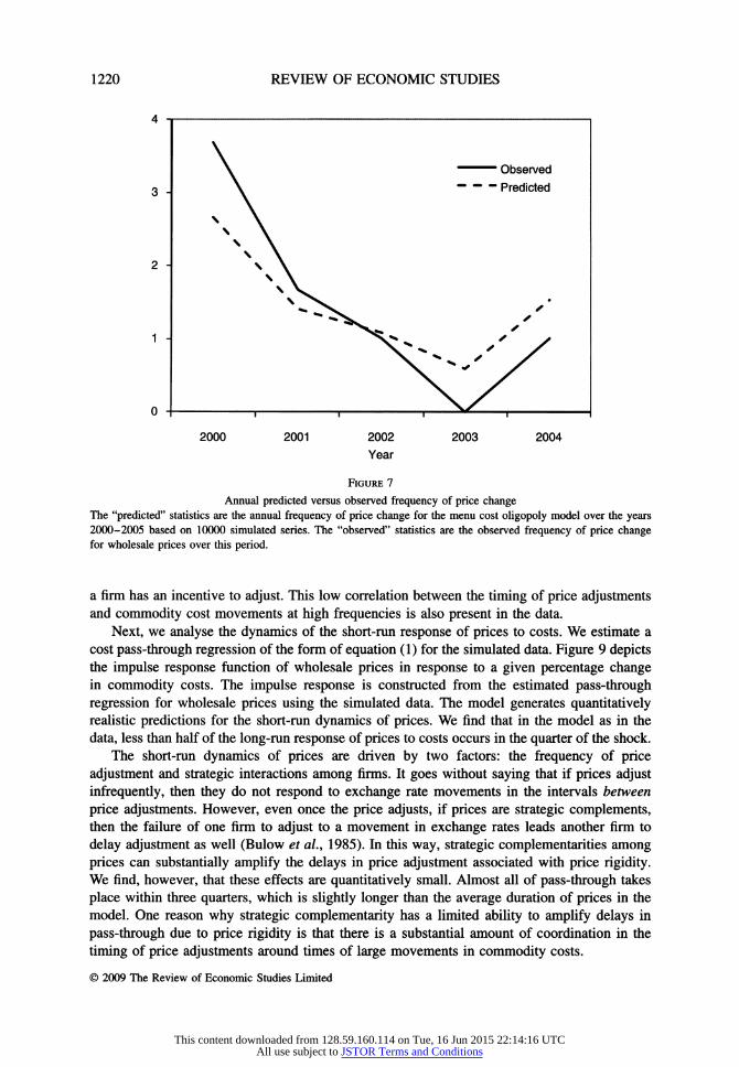
1220 REVIEW OF ECONOMIC STUDIES
4 i »
' ^-^ Observed
3 ' - - - Predicted
' ' ' ' N '
2 - ' ' ' '
0 -I 1 1 1 >^ 1
2000 2001 2002 2003 2004 Year
Figure 7 Annual predicted versus observed frequency of price change
The "predicted" statistics are the annual frequency of price change for the menu cost oligopoly model over the years 2000-2005 based on 10000 simulated series. The "observed" statistics are the observed frequency of price change for wholesale prices over this period.
a firm has an incentive to adjust. This low correlation between the timing of price adjustments and commodity cost movements at high frequencies is also present in the data.
Next, we analyse the dynamics of the short-run response of prices to costs. We estimate a cost pass-through regression of the form of equation (1) for the simulated data. Figure 9 depicts the impulse response function of wholesale prices in response to a given percentage change in commodity costs. The impulse response is constructed from the estimated pass-through regression for wholesale prices using the simulated data. The model generates quantitatively realistic predictions for the short-run dynamics of prices. We find that in the model as in the data, less than half of the long-run response of prices to costs occurs in the quarter of the shock.
The short-run dynamics of prices are driven by two factors: the frequency of price adjustment and strategic interactions among firms. It goes without saying that if prices adjust infrequently, then they do not respond to exchange rate movements in the intervals between price adjustments. However, even once the price adjusts, if prices are strategic complements, then the failure of one firm to adjust to a movement in exchange rates leads another firm to delay adjustment as well (Bulow et al., 1985). In this way, strategic complementarities among prices can substantially amplify the delays in price adjustment associated with price rigidity. We find, however, that these effects are quantitatively small. Almost all of pass-through takes place within three quarters, which is slightly longer than the average duration of prices in the model. One reason why strategic complementarity has a limited ability to amplify delays in pass-through due to price rigidity is that there is a substantial amount of coordination in the timing of price adjustments around times of large movements in commodity costs.
© 2009 The Review of Economic Studies Limited
This content downloaded from 128.59.160.114 on Tue, 16 Jun 2015 22:14:16 UTCAll use subject to JSTOR Terms and Conditions

NAKAMURA & ZEROM ACCOUNTING FOR INCOMPLETE PASS-THROUGH 1221
Annual Freq. Abs. Size
4 -i r 0.028
A -- Freq. Data 3 - '. / ' - 0.023
v ^s* ' - ~ Freq. Model
^^^N. ' -"Abs. Cost Change / 2 - ' ' / 0.018
0 ' ■ J QQQQ
A /
' / V V ' A / '/ v v' V -2 -I L -0.002
2000 2001 2002 2003 2004
Figure 8 Predicted and observed frequency of price change versus absolute cost change
The figure plots the predicted quarterly frequency of price change for the menu cost oligopoly model over the years 2000-2005 (based on 10000 simulated price series) as well as the observed average frequency of wholesale price changes in the data, and the average absolute size of commodity cost changes by quarter.
The model also yields quantitatively realistic predictions for long-run pass-through. The fourth column of Table 8 presents the results of a pass-through regression using the simulated data. Long-run pass-through for the simulated data into retail prices is 0.272 vs. 0.252 in the data. Thus, the model explains almost all of the incomplete pass-through observed in the data.40
It is worth emphasizing that neither the model's fit to the dynamics of pass-through nor its fit to the timing of price adjustments are "guaranteed" by the estimation procedure. The menu costs are estimated based on the frequency of price change over the entire sample period. The demand curve estimation procedure is based purely on the response of consumer demand to fluctuations in prices, the estimation procedure does not make use of information regarding firms' pricing behaviour. The estimates of local costs make use of the average difference between prices and green bean coffee costs over the entire sample period for each product, as well as the demand system estimates, but again do not make use of any information on how prices respond to movements in costs. The implications of the model are also not mechanically "built-in" to the assumed demand curve: the model's implications for pass-through depend on the estimated parameters of the demand curve, menu costs and the oligopolistic market structure.
We next use the dynamic model to investigate the sources of long-run incomplete pass- through. In evaluating this question, the Dixit-Stiglitz demand model serves as a useful
40. A limitation of this model is that it does not explain trade deals, which one would expect to raise pass- through. This effect is likely to be quantitatively small because, as we discuss in Section 3, trade deals are relatively unimportant in explaining cost pass-through.
© 2009 The Review of Economic Studies Limited
This content downloaded from 128.59.160.114 on Tue, 16 Jun 2015 22:14:16 UTCAll use subject to JSTOR Terms and Conditions
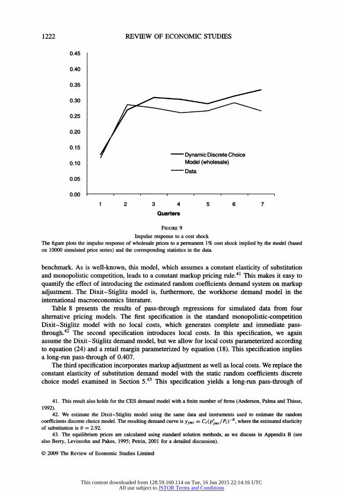
1222 REVIEW OF ECONOMIC STUDIES
0.45
0.40
0.35
0.25 If
0.20 /
0.15 J 7
^^ Dynamic Discrete Choice 0.10 Model (wholesale)
Data 0.05
o.oo I « « 1 1 « 1 1
12 3 4 5 6 7
Quarters
Figure 9
Impulse response to a cost shock The figure plots the impulse response of wholesale prices to a permanent 1% cost shock implied by the model (based on 10000 simulated price series) and the corresponding statistics in the data.
benchmark. As is well-known, this model, which assumes a constant elasticity of substitution and monopolistic competition, leads to a constant markup pricing rule.41 This makes it easy to quantify the effect of introducing the estimated random coefficients demand system on markup adjustment. The Dixit-Stiglitz model is, furthermore, the workhorse demand model in the international macroeconomics literature.
Table 8 presents the results of pass-through regressions for simulated data from four alternative pricing models. The first specification is the standard monopolistic-competition Dixit-Stiglitz model with no local costs, which generates complete and immediate pass- through.42 The second specification introduces local costs. In this specification, we again assume the Dixit-Stiglitz demand model, but we allow for local costs parameterized according to equation (24) and a retail margin parameterized by equation (18). This specification implies a long-run pass-through of 0.407.
The third specification incorporates markup adjustment as well as local costs. We replace the constant elasticity of substitution demand model with the static random coefficients discrete choice model examined in Section 5.43 This specification yields a long-run pass-through of
41. This result also holds for the CES demand model with a finite number of firms (Anderson, Palma and Thisse, 1992).
42. We estimate the Dixit-Stiglitz model using the same data and instruments used to estimate the random coefficients discrete choice model. The resulting demand curve is y;m, = Ct(prjmi/Pt)~6 ', where the estimated elasticity of substitution is 0 = 2.92.
43. The equilibrium prices are calculated using standard solution methods, as we discuss in Appendix B (see also Berry, Levinsohn and Pakes, 1995; Pétrin, 2001 for a detailed discussion).
© 2009 The Review of Economic Studies Limited
This content downloaded from 128.59.160.114 on Tue, 16 Jun 2015 22:14:16 UTCAll use subject to JSTOR Terms and Conditions

NAKAMURA & ZEROM ACCOUNTING FOR INCOMPLETE PASS-THROUGH 1223
TABLE 8 Pass-through regressions for simulated data
Log specification
Variable Dixit-Stiglitz (no Dixit-Stiglitz Static discrete Dynamic discrete local costs) (local costs) choice choice
A Commodity cost (t) 1 0.407 0.213 0.105 A Commodity cost (t - 1) 0 0.028 0.063 0.117 A Commodity cost (t - 2) 0 -0.005 0.025 0.033 A Commodity cost (t - 3) 0 -0.015 0.004 -0.007 A Commodity cost (t - 4) 0 -0.01 1 -0.024 -0.01 1 A Commodity cost (t - 5) 0 0.006 -0.021 0.020 A Commodity cost (t - 6) 0 -0.003 0.014 0.016 Constant 0 0.011 0.009 -0.0008 Long-run pass-through 1 0.407 0.273 0.272
Notes: The dependent variable in all of the specifications is the simulated retail price per ounce in a particular market and quarter. The price and cost variables are in logs. The second column gives the implications of a Dixit-Stiglitz model. The third column gives the implications of a Dixit-Stiglitz model modified to allow for local costs. The fourth column gives the implications of the static discrete choice model, allowing for local costs and markup adjustment. The fifth column gives the implications of the dynamic discrete choice model allowing for local costs, markup adjustment and menu costs.
0.273. Long-run pass-through therefore falls substantially in the discrete choice model relative to the constant elasticity of substitution model. The fourth column adds pricing dynamics in the form of the menu cost model presented in Section 6, causing long-run pass-through to fall to 0.272.
Comparing this set of statistics, we find that local costs reduce long-run pass-through by 59% relative to a CES benchmark, whereas markup adjustment reduces pass-through by an additional 33%. We find that menu costs have a negligible effect on pass-through after six quarters. The result that local costs play a key role in explaining low observed pass-through echoes the conclusions of other industry studies by Goldberg and Verboven (2001), Hellerstein (2008) and Goldberg and Hellerstein (2007), as well as the analysis by Burstein et al (2003) of local costs based on input-output tables. In contrast to Burstein et al. (2003), however, who attribute the entire difference between prices and marginal costs to local costs, our estimated demand pricing model implies that markups are substantial.
Our estimates imply that the markup adjustment in response to cost shocks is considerable in the long-run: firms are estimated to compress their gross margins on average by 1/3 in response to a marginal cost increase. The magnitude of the markup adjustment depends crucially on the curvature of the demand curve. If the elasticity of demand increases as the firm raises its price, the firm is less inclined to raise its price in response to a rise in costs.
One way of summarizing this curvature is in terms of the estimated "super-elasticity" of demand, the percentage change in the price elasticity for a given percentage increase in prices (Klenow and Willis, 2006). This super-elasticity is zero by assumption in the Dixit-Stiglitz model. In contrast, an advantage of the random coefficients demand system we consider is that it permits a great deal of flexibility in the specification of the curvature of demand. Our estimated demand curve, which implies a super-elasticity of demand of 4.64, generates a substantial motive for markup adjustment. Depending on the parameters used, however, the random coefficients demand system can generate a wide variety of possible curvatures of demand, and therefore, a wide variety of potential implications for pass-through. We investigate how our results vary for alternative parameterizations of the demand curve in Section 8.
© 2009 The Review of Economic Studies Limited
This content downloaded from 128.59.160.114 on Tue, 16 Jun 2015 22:14:16 UTCAll use subject to JSTOR Terms and Conditions
1224 REVIEW OF ECONOMIC STUDIES
Finally, our estimates imply that menu costs have almost no impact on long-run pass-through. In this regard, our results contrast with a large literature in international macroeconomics in which sticky prices play a central role in lowering the responsiveness of prices to exchange rates (see, for example, Engel, 2002). This conclusion depends importantly on the dynamics of marginal costs, as we discuss in the next section.
8. COUNTERFACTUAL EXPERIMENTS
We next carry out a quantitative investigation of a number of the factors discussed above, the volatility and persistence of costs, the timing of price adjustments and the curvature of demand, in explaining the short-run and long-run dynamics of pass-through. We do this by repeating the types of quantitative experiments we carried out above for various alternative parameter values.
We first investigate how pass-through depends on the persistence of marginal costs. To do this, we consider counterfactual experiments where we hold fixed the actual sequence of costs faced by the firms, but make different assumptions about what firms believe regarding the stochastic process generating marginal costs (i.e. equation (20)). The menu cost is adjusted to hold the frequency of price change in each simulation equal to the observed frequency of price change.
Table 9 (columns 3 and 4) presents pass-through regressions for cases where pc = 0.9 and pc =0.5. The variance and constant term in the alternative cost processes are chosen to match the corresponding unconditional statistics in the data. Quantitatively, the persistence of marginal costs has a substantial role in determining long-run pass-through. As we move from the baseline specification in which costs have a unit root to the case with pc =0.5, the long-run pass-through drops from 0.272 (the baseline case) to 0.161. Even for the case with pc = 0.9, the pass-through is 0.210, which is substantially lower than in the baseline specification. Intuitively, firms adjust incompletely to changes in costs even over the longer horizon because they expect costs to revert to some "normal" level. This effect does not arise in the case where marginal costs have a unit root.
Second, we consider how the timing of price changes implied by the menu cost model affects pass-through. We compare pass-through in the menu cost model to pass-through in the Calvo (1983) model in which the timing of price changes is random. The Calvo model is a workhorse of the macroeconomics and international economics literatures. In the Calvo specification, we assume that instead of facing a menu cost as in the model in Section 6, firms are randomly selected to adjust their prices with probability a calvo- We choose a calvo to fit the observed frequency of price change as in the other simulations. Otherwise, the model is unchanged, and has the same parameterization as the baseline model.
Table 9 (columns 5 and 6) presents the results of pass-through regressions for the Calvo model. The baseline Calvo model implies substantially more delayed pass-through than the menu cost model: only about 25% of pass-through occurs in the first quarter on average compared with an average of 40% in the menu cost model. This difference arises because, in the menu cost model, prices adjust rapidly to large and persistent cost shocks. Table 9 also presents results for the Calvo model with pc = 0.9. Lowering the persistence of costs has an even greater effect on the results for the Calvo model than for the menu cost model: the long-run pass-through falls from 0.272 in the baseline specification to 0.162 in the specification with lower persistence.
Third, we investigate how the predictions of our model depend on the curvature of demand. In our structural model of demand, the key parameters that determine the curvature of demand are those that relate to the degree of consumer heterogeneity. The literature on differentiated
© 2009 The Review of Economic Studies Limited
This content downloaded from 128.59.160.114 on Tue, 16 Jun 2015 22:14:16 UTCAll use subject to JSTOR Terms and Conditions
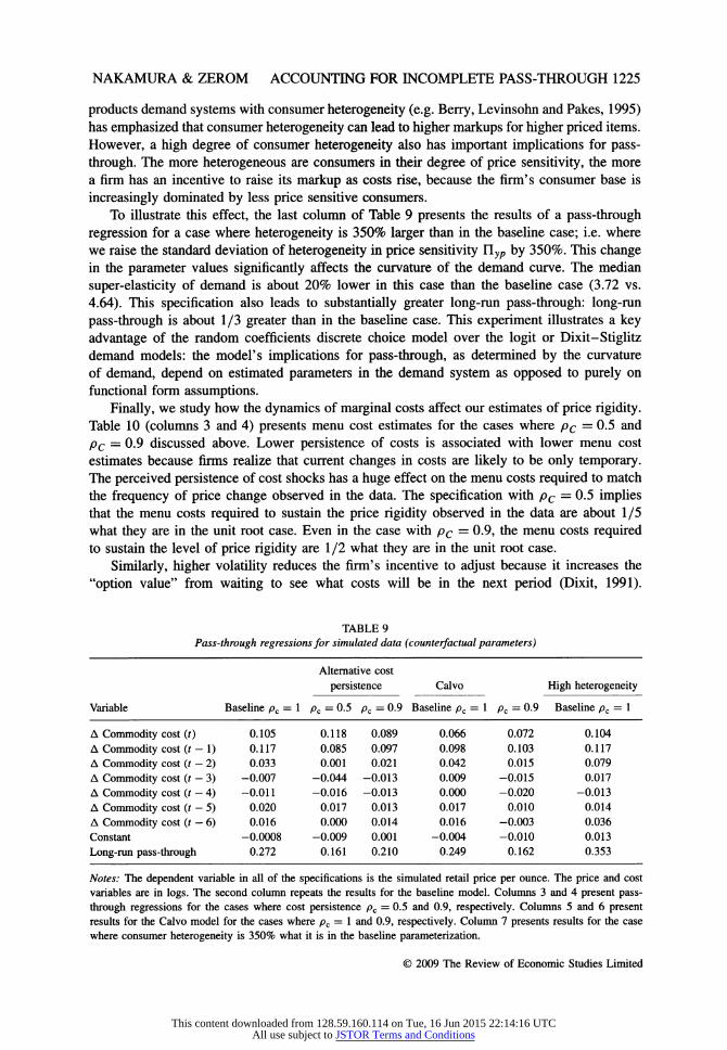
NAKAMURA & ZEROM ACCOUNTING FOR INCOMPLETE PASS-THROUGH 1225
products demand systems with consumer heterogeneity (e.g. Berry, Levinsohn and Pakes, 1995) has emphasized that consumer heterogeneity can lead to higher markups for higher priced items. However, a high degree of consumer heterogeneity also has important implications for pass- through. The more heterogeneous are consumers in their degree of price sensitivity, the more a firm has an incentive to raise its markup as costs rise, because the firm's consumer base is increasingly dominated by less price sensitive consumers.
To illustrate this effect, the last column of Table 9 presents the results of a pass-through regression for a case where heterogeneity is 350% larger than in the baseline case; i.e. where we raise the standard deviation of heterogeneity in price sensitivity Ylyp by 350%. This change in the parameter values significantly affects the curvature of the demand curve. The median super-elasticity of demand is about 20% lower in this case than the baseline case (3.72 vs. 4.64). This specification also leads to substantially greater long-run pass-through: long-run pass-through is about 1/3 greater than in the baseline case. This experiment illustrates a key advantage of the random coefficients discrete choice model over the logit or Dixit-Stiglitz demand models: the model's implications for pass-through, as determined by the curvature of demand, depend on estimated parameters in the demand system as opposed to purely on functional form assumptions.
Finally, we study how the dynamics of marginal costs affect our estimates of price rigidity. Table 10 (columns 3 and 4) presents menu cost estimates for the cases where pc = 0.5 and pc = 0.9 discussed above. Lower persistence of costs is associated with lower menu cost estimates because firms realize that current changes in costs are likely to be only temporary. The perceived persistence of cost shocks has a huge effect on the menu costs required to match the frequency of price change observed in the data. The specification with pc = 0.5 implies that the menu costs required to sustain the price rigidity observed in the data are about 1/5 what they are in the unit root case. Even in the case with pc = 0.9, the menu costs required to sustain the level of price rigidity are 1/2 what they are in the unit root case.
Similarly, higher volatility reduces the firm's incentive to adjust because it increases the "option value" from waiting to see what costs will be in the next period (Dixit, 1991).
TABLE 9 Pass-through regressions for simulated data (counter/actual parameters)
Alternative cost persistence Calvo High heterogeneity
Variable Baseline pc = 1 pc = 0.5 pc = 0.9 Baseline pc = 1 pc = 0.9 Baseline pc = 1
A Commodity cost (0 0.105 0.118 0.089 0.066 0.072 0.104 A Commodity cost (t - 1) 0.117 0.085 0.097 0.098 0.103 0.117 A Commodity cost (t - 2) 0.033 0.001 0.021 0.042 0.015 0.079 A Commodity cost {t - 3) -0.007 -0.044 -0.013 0.009 -0.015 0.017 A Commodity cost (t - 4) -0.011 -0.016 -0.013 0.000 -0.020 -0.013 A Commodity cost {t - 5) 0.020 0.017 0.013 0.017 0.010 0.014 A Commodity cost (t - 6) 0.016 0.000 0.014 0.016 -0.003 0.036 Constant -0.0008 -0.009 0.001 -0.004 -0.010 0.013 Long-run pass-through 0.272 0.161 0.210 0.249 0.162 0.353
Notes: The dependent variable in all of the specifications is the simulated retail price per ounce. The price and cost variables are in logs. The second column repeats the results for the baseline model. Columns 3 and 4 present pass- through regressions for the cases where cost persistence pc = 0.5 and 0.9, respectively. Columns 5 and 6 present results for the Calvo model for the cases where pc = 1 and 0.9, respectively. Column 7 presents results for the case where consumer heterogeneity is 350% what it is in the baseline parameterization.
© 2009 The Review of Economic Studies Limited
This content downloaded from 128.59.160.114 on Tue, 16 Jun 2015 22:14:16 UTCAll use subject to JSTOR Terms and Conditions

1226 REVIEW OF ECONOMIC STUDIES
TABLE 10 Menu cost estimates ( counte rf actual parameters)
Alternative persistence Alternative volatility parameters parameters Static model
Baseline pc = 1 pc = 0.5 pc = 0.9 Low volatility High volatility Discount factor = 0
Menu cost 0.22 0.049 0.11 0.33 0.13 0.065 estimate (%)
Notes: The table presents menu cost estimates as a fraction of average annual firm revenue in the Syracuse market. The second column repeats the baseline results. Columns 3-7 present results for counterfactual parameter values. Columns 3 and 4 present results for the cases where pc = 0.5 and 0.9, respectively. Columns 5 and 6 present results for the low- and high-volatility cases described in the text. Column 7 presents results for a case where ß = 0, that is, there is no forward-looking behaviour.
Columns 5 and 6 present the menu costs required to match the observed price rigidity for cases where the standard deviation of cost shocks a2c is assumed to be higher or lower than in the baseline case. Quantitatively, the option value effects are substantial. Lowering the standard deviation of costs to half the baseline case implies that the required menu costs are 150% what they are in the baseline case; while raising the standard deviation to twice what it is in the baseline case implies menu costs that are about 50% of the baseline value.
One approximation that has sometimes been used in the industrial organization and international economics literatures to evaluate the magnitude of barriers to price adjustment is to compare the profits from fixed prices to profits when prices are set at the static optimum in every period (e.g. Leslie, 2004; Goldberg and Hellerstein, 2007). One can evaluate the effects of this type of approximation by considering a static version of the model with the discount factor ß set to zero. In this case, the firm simply compares the static profits from adjusting to the menu cost in each period. The last column of Table 10 shows that this procedure yields a menu cost estimate that is only 30% of what it is in the dynamic model with forward-
looking behaviour. The static procedure underestimates the magnitude of menu costs because it overlooks the fact that in deciding whether to adjust, the firm not only considers benefits
today but also benefits in the future. These benefits are substantial when costs are persistent. Thus, menu cost estimates based on static procedures are likely to be substantially lower than estimates from dynamic models when costs are persistent.44
9. CONCLUSION
A large literature in international economics studies the response of domestic prices to fluctuations in imported costs. We use data on coffee prices at the retail, wholesale and commodity cost levels to study how variations in the price of imported inputs translate into
changes in downstream prices. For both retail and wholesale prices, we find that pass-through is delayed and incomplete. Reduced-form regressions indicate the delayed response of prices to costs in this industry occurs almost entirely at the wholesale level. We show that a menu cost model parameterized to match the observed degree of wholesale price rigidity can match the basic facts of price adjustment in this industry: infrequent price adjustments, the strong tendency of prices to adjust more frequently in periods when commodity costs experience
44. In contrast, when costs are not persistent (e.g. the pc = 0 case), the menu cost estimate based on the dynamic analysis may be lower than the estimate based on a static analysis because the static analysis also ignores the "option value" associated with not adjusting.
© 2009 The Review of Economic Studies Limited
This content downloaded from 128.59.160.114 on Tue, 16 Jun 2015 22:14:16 UTCAll use subject to JSTOR Terms and Conditions
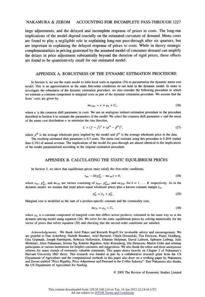
NAKAMURA & ZEROM ACCOUNTING FOR INCOMPLETE PASS-THROUGH 1227
large adjustments, and the delayed and incomplete response of prices to costs. The long-run implications of the model depend crucially on the estimated curvature of demand. Menu costs are found to play a negligible role in explaining long-run pass-through after six quarters, but are important in explaining the delayed response of prices to costs. While in theory strategic complementarities in pricing generated by the assumed model of consumer demand can amplify the delays in price adjustment substantially beyond the duration of rigid prices, these effects are found to be quantitatively small for our estimated model.
APPENDIX A. ROBUSTNESS OF THE DYNAMIC ESTIMATION PROCEDURE
In Section 6, we use the static model to infer local costs in equation (24) to parameterize the dynamic menu cost model. This is an approximation as the static first-order conditions do not hold in the dynamic model. In order to investigate the robustness of the dynamic estimation procedure, we also consider the following procedure in which we estimate a common component in marginal costs as part of the dynamic estimation procedure. We assume that the firms' costs are given by,
mckmt =K + fik + Cti (26)
where k is the common shift parameter in costs. We use an analogous indirect estimation procedure to the procedure described in Section 6 to estimate the parameters of the model. We select the common shift parameter k and the mean of the menu cost distribution a to minimize the loss function,
¿ = (/-/)2 + (/>"-p")2. (27)
where pw is the average wholesale price implied by the model and pw is the average wholesale price in the data. The resulting estimated shift parameter is 0.3 cents. The menu cost estimate using this procedure is 0.26% (rather
than 0.3%) of annual revenue. The implications of the model for pass-through are almost identical to the implications of the model parameterized according to the original estimation procedure.
APPENDIX B. CALCULATING THE STATIC EQUILIBRIUM PRICES
In Section 5, we show that equilibrium prices must satisfy the first-order conditions,
smt-Q(pZ-mcmt)=0, (28)
where smt, p%n and mcmt are vectors consisting of skmt, p™mt, and mckmt for k = 1, . . . , K respectively. As in the dynamic model, we assume that retail prices equal wholesale prices plus a known constant margin £¿,
Pi, = ft + /»",- (29)
Marginal cost is modelled as the sum of a product-specific constant and the commodity cost,
fnckt = ßk + Ct, (30)
where ßk is a constant component of marginal costs that differs across products, estimated in the same way as in the dynamic pricing model using equation (24). We solve for the static equilibrium prices by solving numerically for the vector of prices that solves equation (28) and checking that the second-order conditions are satisfied.
Acknowledgements. We thank Ariel Pakes and Kenneth Rogoff for invaluable advice and encouragement. We are grateful to Dan Ackerberg, Hafedh Bouakez, Ariel Burstein, Ulrich Dorazelski, Tim Erickson, Penny Goldberg, Gita Gopinath, Joseph Harrington, Rebecca Hellerstein, Elhanan Helpman, David Laibson, Ephraim Leibtag, Julie Mortimer, Alice Nakamura, Serena Ng, Roberto Rigobon, Julio Rotemberg, Jón Steinsson, Martin Uribe and seminar participants at various institutions for helpful comments and suggestions. We also thank the editor and three anonymous referees for many rounds of extremely valuable comments. This paper draws heavily on Chapter 2 of Nakamura' s Harvard University PhD thesis. This research was funded in part by a collaborative research grant from the US Department of Agriculture and the computational methods in this paper also draw on a working paper by Nakamura and Zerom entitled "Price Rigidity, Price Adjustment and Demand in the Coffee Industry". Emi Nakamura also thanks the US Department of Agriculture for funding.
© 2009 The Review of Economic Studies Limited
This content downloaded from 128.59.160.114 on Tue, 16 Jun 2015 22:14:16 UTCAll use subject to JSTOR Terms and Conditions
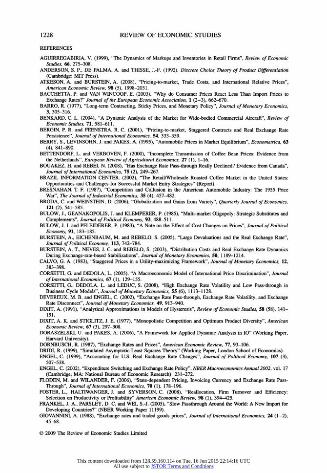
1228 REVIEW OF ECONOMIC STUDIES
REFERENCES
AGUIRREGABIRIA, V. (1999), "The Dynamics of Markups and Inventories in Retail Firms", Review of Economic Studies, 66, 275-308.
ANDERSON, S. P., DE PALMA, A. and THISSE, J.-F. (1992), Discrete Choice Theory of Product Differentiation (Cambridge: MIT Press).
ATKESON, A. and BURSTEIN, A. (2008), "Pricing-to-market, Trade Costs, and International Relative Prices", American Economic Review, 98 (5), 1998-2031.
BACCHETTA, P. and VAN WINCOOP, E. (2003), "Why do Consumer Prices React Less Than Import Prices to Exchange Rates?" Journal of the European Economic Association, 1 (2-3), 662-670.
BARRO, R. (1977), "Long-term Contracting, Sticky Prices, and Monetary Policy", Journal of Monetary Economics, 3, 305-316.
BENKARD, C. L. (2004), "A Dynamic Analysis of the Market for Wide-bodied Commercial Aircraft", Review of Economic Studies, 71, 581-611.
BERGIN, P. R. and FEENSTRA, R. C. (2001), "Pricing-to-market, Staggered Contracts and Real Exchange Rate Persistence", Journal of International Economics, 54, 333-359.
BERRY, S., LEVINSOHN, J. and PAKES, A. (1995), "Automobile Prices in Market Equilibrium", Econometrica, 63 (4), 841-890.
BETTENDORF, L. and VERBOVEN, F. (2000), "Incomplete Transmission of Coffee Bean Prices: Evidence from the Netherlands", European Review of Agricultural Economics, 27 (1), 1-16.
BOUAKEZ, H. and REBEI, N. (2008), "Has Exchange Rate Pass-through Really Declined? Evidence from Canada", Journal of International Economics, 75 (2), 249-267.
BRAZIL INFORMATION CENTER. (2002), "The Retail/Wholesale Roasted Coffee Market in the United States: Opportunities and Challenges for Successful Market Entry Strategies" (Report).
BRESNAHAN, T. F. (1987), "Competition and Collusion in the American Automobile Industry: The 1955 Price War", The Journal of Industrial Economics, 35 (4), 457^82.
BRODA, C. and WEINSTEIN, D. (2006), "Globalization and Gains from Variety", Quarterly Journal of Economics, 121 (2), 541-585.
BULOW, J., GEANAKOPOLIS, J. and KLEMPERER, P. (1985), "Multi-market Oligopoly: Strategic Substitutes and Complements", Journal of Political Economy, 93, 488-511.
BULOW, J. I. and PFLEIDERER, P. (1983), "A Note on the Effect of Cost Changes on Prices", Journal of Political Economy, 91, 183-185.
BURSTEIN, A., EICHENBAUM, M. and REBELO, S. (2005), "Large Devaluations and the Real Exchange Rate", Journal of Political Economy, 113, 742-784.
BURSTEIN, A. T., NEVES, J. C. and REBELO, S. (2003), "Distribution Costs and Real Exchange Rate Dynamics During Exchange-rate-based Stabilizations", Journal of Monetary Economics, 50, 1189-1214.
CALVO, G. A. (1983), "Staggered Prices in a Utility-maximizing Framework", Journal of Monetary Economics, 12, 383-398.
CORSETTI, G. and DEDOLA, L. (2005), "A Macroeconomic Model of International Price Discrimination", Journal of International Economics, 67 ( 1 ), 1 29- 155.
CORSETTI, G., DEDOLA, L. and LEDUC, S. (2008), "High Exchange Rate Volatility and Low Pass-through in Business Cycle Models", Journal of Monetary Economics, 55 (6), 1113-1128.
DEVEREUX, M. B. and ENGEL, C. (2002), "Exchange Rate Pass-through, Exchange Rate Volatility, and Exchange Rate Disconnect", Journal of Monetary Economics, 49, 913-940.
DIXIT, A. (1991), "Analytical Approximations in Models of Hysteresis", Review of Economic Studies, 58 (58), 141- 151.
DIXIT, A. K. and STIGLITZ, J. E. (1977), "Monopolistic Competition and Optimum Product Diversity", American Economic Review, 67 (3), 297-308.
DORASZELSKI, U. and PAKES, A. (2006), "A Framework for Applied Dynamic Analysis in IO" (Working Paper, Harvard University).
DORNBUSCH, R. (1987), "Exchange Rates and Prices", American Economic Review, 77, 93-106. DRIDI, R. (1999), "Simulated Asymptotic Least Squares Theory" (Working Paper, London School of Economics). ENGEL, C. (1999), "Accounting for U.S. Real Exchange Rate Changes", Journal of Political Economy, 107 (3),
507-538. ENGEL, C. (2002), "Expenditure Switching and Exchange Rate Policy", NBER Macroeconomics Annual 2002, vol. 17
(Cambridge, MA: National Bureau of Economic Research) 231-272. FLODEN, M. and WILANDER, F. (2006), "State-dependent Pricing, Invoicing Currency and Exchange Rate Pass-
Through", Journal of International Economics, 70 (1), 178-196. FOSTER, L., HALTIWANGER, J. and SYVERSON, C. (2008), "Reallocation, Firm Turnover and Efficiency:
Selection on Productivity or Profitability" American Economic Review, 98 (1), 394-425. FRANKEL, J. A., PARSLEY, D. C. and WEI, S.-J. (2005), "Slow Passthrough Around the World: A New Import for
Developing Countries?" (NBER Working Paper 11199). GIO VANNINI, A. (1988), "Exchange rates and traded goods prices", Journal of International Economics, 24 (1-2),
45-68.
© 2009 The Review of Economic Studies Limited
This content downloaded from 128.59.160.114 on Tue, 16 Jun 2015 22:14:16 UTCAll use subject to JSTOR Terms and Conditions
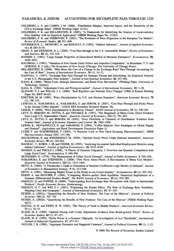
NAKAMURA & ZEROM ACCOUNTING FOR INCOMPLETE PASS-THROUGH 1229
GOLDBERG, L. S. and CAMPA, J. M. (2006), "Distribution Margins, Imported Inputs, and the Sensitivity of the CPI to Exchange Rates" (NBER Working Paper 12121).
GOLDBERG, P. K. and HELLERSTEIN, R. (2007), "A Framework for Identifying the Sources of Local-currency Price Stability with an Empirical Application" (NBER Working Paper No. 13183).
GOLDBERG, P. K. and VERBOVEN, F. (2001), 'The Evolution of Price Dispersion in the European Car Market", Review of Economic Studies, 68, 811-848.
GOURIEROUX, C, MONFORT, A. and RENAULT, E. (1993), "Indirect Inference", Journal of Applied Economet- rics, 8, S85-S118.
GRON, A. and SWENSON, D. L. (2000), "Cost Pass-through in the U.S. Automobile Market", Review of Economics and Statistics, 82 (2), 316-324.
HANSEN, L. (1982), "Large Sample Properties of Generalized Method of Moments Estimators", Econometrica, 50, 1029-1054.
HAUSMAN, J. (1997), "Valuation of New Goods Under Perfect and Imperfect Competition", in Bresnahan, T. F. and GORDON, R. J. (eds.) The Economics of New Goods (Chicago: The University of Chicago Press).
HELLERSTEIN, R. (2008), "Who Bears the Cost of a Change in the Exchange Rate? Pass-Through Accounting for the Case of Beer", Journal of International Economics, 76 (1), 14-32.
KADIYALI, V. (1997), "Exchange Rate Pass-Through for Strategic Pricing and Advertising: An Empirical Analysis of the U.S. Photographic Film Industry", Journal of International Economics, 43, 437-461.
KANO, K. (2006), "Menu Costs, Strategic Interactions, and Retail Price Movements" (Working Paper, University of Technology, Sydney).
KASA, K. (1992), "Adjustment Costs and Pricing-to-market", Journal of International Economics, 32, 1-30. KLENOW, P. J. and WILLIS, J. L. (2006), "Real Rigidities and Nominal Price Changes" (FRB of Kansas Working
Paper No. RWP 06-03). KNETTER, M. M. (1989), "Price Discrimination by U.S. and German Exporters", American Economic Review, 79
(1), 198-210. LEIBTAG, E., NAKAMURA, A., NAKAMURA, E. and ZEROM, D. (2007), "Cost Pass-Through and Sticky Prices
in the Ground Coffee Industry", (USDA ERS Economic Research Report, 38). LESLIE, P. (2004), "Price Discrimination in Broadway Theatre", RAND Journal of Economics, 35 (3), 520-541. LEVY, D., BERGEN, M., DUTTA, S. and VENABLE, R. (1997), "The Magnitude of Menu Costs: Direct Evidence
from Large U.S. Supermarket Chains", Quarterly Journal of Economics, 112 (3), 791-825. LEVY, D., DUTTA, S. and BERGEN, M. (2002), "Price Flexibility in Channels of Distribution: Evidence from
Scanner Data", Journal of Economic Dynamics and Control, 26, 1845-1900. LEWIN, B., GIOVANNUCCI, D. and VARANGIS, P. (2004), "Coffee Markets: New Paradigms in Global Supply
and Demand", (Agriculture and Rural Development Discussion Paper 3). LUBIK T. and SCHORFHEIDE, F. (2005), "A Bayesian Look at New Open Economy Macroeconomics", NBER
Macroeconomics Annual 2005, 313-366. MACKOWIAK, B. and WIEDERHOLT, M. (2009), "Optimal Sticky Prices Under Rational Inattention", American
Economic Review, 99 (3), 769-803. MAGNAC, T., ROBIN, J.-M. and VISSER, M. (1995), "Analysing Incomplete Individual Employment Histories using
Indirect Inference", Journal of Applied Econometrics, 10, S153-S169. MAS KIN, E. and TIRÓLE J. (1988), "A Theory of Dynamic Oligopoly, I: Overview and Quantity Competition with
Large Fixed Costs", Econometrica, 3, 549-569. MCFADDEN, D. (1974), "The Measurement of Urban Travel Demand", Journal of Public Economics, 3, 303-328. NAKAMURA, E. and STEINSSON, J. (2008), "Five Facts About Prices: A Réévaluation of Menu Cost Models",
Quarterly Journal of Economics, 123 (4), 1415-1464. NEVO, A. (2000), "A Practitioner's Guide to Estimation of Random Coefficients Logit Models of Demand", Journal
of Economics & Management Strategy, 9 (4), 513-548. NEVO, A. (2001), "Measuring Market Power in the Ready-to-eat Cereal Industry", Econometrica, 69 (2), 307-342. PAKES, A. and McGUIRE, P. (1994), "Computing Markov-perfect Nash Equilibria: Numerical Implications of a
Dynamic Differentiated Product Model", The RAND Journal of Economics, 25 (4), 555-589. PARSLEY, D. and POPPER, H. (2009), "Understanding Real Exchange Rate Movements with Trade in Intermediate
Products", Pacific Economic Review, (forthcoming). PARSLEY, D. C. and WEI, S.-J. (2001), "Explaining the Border Effect: The Role of Exchange Rate Variability,
Shipping Costs and Geography", Journal of International Economics, 55, 87-105. PETRIN, A. (2002«), "Quantifying the Benefits of New Products: The Case of the Minivan", Journal of Political
Economy, 110 (4), 705-729. PETRIN, A. (20026), "Quantifying the Benefits of New Products: The Case of the Minivan" (NBER Working Paper
8227). SANYAL, K. K. and JONES, R. W. (1982), "The Theory of Trade in Middle Products", American Economic Review,
72 (1), 16-31. SLADE, M. E. (1998), "Optimal Pricing with Costly Adjustment: Evidence from Retail-grocery Prices", Review of
Economic Studies, 65 (1), 87-107. SLADE, M. E. (1999), "Sticky Prices in a Dynamic Oligopoly: An Investigation of (s,s) Thresholds", International
Journal of Industrial Organization, 17, 477-511. TAYLOR, J. B. (1980), "Aggregate Dynamics and Staggered Contracts", Journal of Political Economy, 88 (1), 1-23.
© 2009 The Review of Economic Studies Limited
This content downloaded from 128.59.160.114 on Tue, 16 Jun 2015 22:14:16 UTCAll use subject to JSTOR Terms and Conditions
1230 REVIEW OF ECONOMIC STUDIES
VILLAS-BOAS, S. B. (2007), "Vertical Relationships between Manufacturers and Retailers: Inference with Limited Data", Review of Economic Studies, 74 (2), 625-652.
YIP, G. S. and WILLIAMS, J. R. (1985), U.S. retail coffee market (B). HBS Case 582-088,. ZBARACKI, M. J., RTTSON, M., LEVY, D., DUTTA, S. and BERGEN, M. (2004), "Managerial and Customer Costs
of Price Adjustment: Direct Evidence from Industrial Markets", The Review of Economics and Statistics, 86 (2), 514-533.
© 2009 The Review of Economic Studies Limited
This content downloaded from 128.59.160.114 on Tue, 16 Jun 2015 22:14:16 UTCAll use subject to JSTOR Terms and Conditions