Accounting Conservatism and the Temporal Trends in Current

Earnings’ Ability to Predict Future Cash Flows versus Future Earnings:

Evidence on the Trade-off between Relevance and Reliability

Sati P. Bandyopadhyay, Changling Chen**, Alan G. Huang, and Ranjini Jha

*All authors are from the School of Accounting and Finance, University of Waterloo, Waterloo, Ontario, Canada, N2L 3Gl. emails: Bandyopadhyay, bandy@uwaterloo.ca; Chen, clchen@uwaterloo.ca; Huang, aghuang@uwaterloo.ca; and Jha, rjha@uwaterloo.ca. We thank participants at the 2008 CAAA meetings and the 2008 CAR conference, Edward Riedl, the discussant at the CAR conference, Jeffery Callen (the associate editor), and two anonymous referees. All errors remain ours.

**Contact author: Address correspondence to Changling Chen: Phone: 519-888-4567 ext. 35731; fax: 519-888-7562; email: clchen@uwaterloo.ca.

1

Accounting Conservatism and the Temporal Trends in Current

Earnings’ Ability to Predict Future Cash Flows versus Future Earnings:

Evidence on the Trade-off between Relevance and Reliability

Abstract

This research reports that an increasing level of accounting conservatism over the 1973–2005 period is associated with (1) an increase in the ability of current earnings to predict future cash flows (a measure of relevance, e.g., Kim and Kross, 2005); and (2) a decrease in the ability of current earnings to predict future earnings (a measure of reliability in the Richardson et al. [2005] sense). We also find that usefulness of earnings for explaining stock prices over book values is positively related to reliability but not to relevance. Our results hold for the constant and full samples and in both in-sample and out-of-sample analyses and are also robust to the use of different measures for relevance, reliability, earnings usefulness, and conservatism. Our findings about the relations between conservatism, relevance, reliability, and usefulness suggest a trade-off between relevance and reliability and seem to indicate that the adoption of an increasing number of conservative accounting standards possibly has an adverse impact on earnings usefulness through their negative effects on reliability. Key Words: Relevance, Reliability, Earnings Predictability, Cash Flow

Predictability, Earnings Usefulness and Accounting Conservatism

JEL: M41, C23, D21, G38, N20

2

1. INTRODUCTION

Several recent papers find that the usefulness of earnings for explaining

contemporaneous stock prices has been declining over time.1 In particular, Collins et al.

(1997, table 3) show that the incremental R2 of earnings for explaining stock prices over

book values (a proxy of earnings usefulness) declined from a high of 30% during 1953–

1962 to approximately 7% during 1983–1993. Kim and Kross (2005, table 4) find the

relation to have further deteriorated to 5.7% during 1992–2000. These authors also report

that the ability of current earnings to predict future operating cash flows more than

doubled during the same period. Because stock price is the present value of future cash

flows, this intertemporal decline in earnings usefulness is called “puzzling” and

“incongruous” (Barth, Cram and Nelson, 2001, p30; Kim and Kross, 2005, p754).

In this paper we examine the Kim and Kross (2005) puzzle by focusing on an idea

proposed by these authors themselves that the “earnings price relationship might decline

even in the absence of a decline in the relationship between earnings and future cash

flows if, for example, the market forecasts a dramatic drop in persistence.”2 We find that

this is indeed the case.3 More interestingly, in this paper we show that increasing

accounting conservatism over the past 30 years has contributed to the decline in earnings

usefulness by its divergent effects on current earnings’ ability to predict (i) future cash

flows and (ii) future earnings. Consistent with the findings of Kim and Kross (2005), we

provide evidence that accounting conservatism enhances the predictive ability of current

1 See, e.g., Amir and Lev (1996), Collins, Maydew and Weiss (1997), Brown, Lo and Lys (1999), and Francis and Schipper (1999). In addition, Kim and Kross (2005) provide an exhaustive list of related studies. 2 For example, Dichev and Tang (2006) document declining earnings persistence over the past 30 years. 3 Several authors also have provided evidence that earnings usefulness is positively correlated with the ability of current earnings to predict future earnings or earnings persistence (Kormendi and Lipe 1987, Collins and Kothari 1989, Easton and Zmijewski 1989, Lipe 1990).

3

earnings for future cash flows. In contrast, we find that conservatism reduces the

predictive ability of current earnings for future earnings (or persistence). The final result

is a decline in earnings usefulness arising from the trade-off between future cash flow

predictability and earnings persistence.

The trade-off referred to in the previous paragraph is similar in spirit to the

relevance-reliability trade-off, referred to in SFAC No.2. Kim and Kross (2005, p778)

consider earnings “relevance” as “the ability of earnings in year t to forecast the operating

cash flows (CFO) in year t + 1.” The predictive notion of future cash flow is consistent

with the definition of “relevance” in SFAC No. 2 (paragraph 57), namely, “prediction of

outcomes.” As far as reliability is concerned, Richardson et al. (2005) argue that the

SFAC 2 definition of reliability, “The quality of information that assures that information

is reasonably free from error and bias and faithfully represents what it purports to

represent,” provides a link between accrual reliability and earnings persistence. They

suggest earnings persistence as a proxy for reliability based on the argument that

measurement error in accounting accruals imparts potential error in the earnings

measurement process and thereby lowers the correlation between current earnings and

future earnings (earnings persistence). The greater the magnitude of measurement error in

current earnings, the lower is the correlation between current earnings and future

earnings, and this leads to lower earnings persistence. Kirschenheiter (1997, p50) also

adopts a similar approach to reliability. He suggests that reliability is linked to the

estimation process in accounting measurements and is measured by the “precision of an

estimate.” Consistent with the foregoing measurement error perspective, we attempt to

capture the notion of “reliability” by the ability of current earnings’ to predict future

4

earnings, although admittedly this is a “predictive” notion, which does not map perfectly

into SFAC No. 2. Our inferences are subject to this caveat.

Our study of the interaction between conservatism and the relevance-reliability

trade-off is grounded in the properties of conservative accounting. Givoly and Hayn

(2000) provide evidence that earnings recognition has become more conservative in the

past several decades. They attribute this increase to the result of application of numerous

FASB pronouncements that require early recognition of expenses and anticipated future

losses in income and the deferral of gains until they are realized (see Givoly and Hayn,

2000, footnote 1), which is a probable cause for the increasing ability of current earnings

to predict future cash flows (Kim and Kross, 2005). This is consistent with increasing

conservatism enhancing “relevance” of earnings numbers. Alternatively, estimating

future anticipated losses (conservative accounting) might impart measurement error and

bias into accounting accruals arising from the uncertainty about the amount of accruals

that will be recognized in earnings. This uncertainty imparts potential measurement error

into accruals and hence into earnings because earnings equal cash flows plus accruals,

thereby lowering earnings persistence (Richardson et al. 2005) and hence usefulness with

which earnings persistence is positively correlated (see footnote 3). The foregoing

discussion speaks to a possible trade-off between future cash flow predictability

(relevance) versus future earnings predictability (reliability) of current earnings. To

summarize, here we examine two empirical issues: (1) the effect of accounting

conservatism on the trade-off between future earnings predictability (hereafter,

reliability) versus future cash flow predictability (hereafter, relevance) of current

earnings, and (2) the effect of this trade-off on earnings usefulness.

5

We focus on two different samples in tandem to examine the linkages between

these earnings attributes, namely, earnings usefulness, accounting conservatism,

relevance, and reliability. The first sample is the “full sample” of 97,332 firm-years of

observations during our sample period of 1973–2005. The second is a subset of the first

sample, namely, a “constant sample” of 448 firms that survive most of the sample period.

In the second sample, firms are held constant each year while the accounting environment

changes over time. Hence, the second sample achieves better control of the firm specific

factors that might affect the earnings attributes examined in this paper.

Our primary measures of earnings usefulness, reliability and relevance are based

on the incremental R2 approach (in-sample) and the Theil’s U statistic (out-of-sample)

used in prior related literature such as Collins et al. (1997) and Kim and Kross (2005).

We use two different measures of accounting conservatism in our empirical tests, namely,

cumulative nonoperating accruals and an index created from four different conservatism

measures used in Givoly and Hayn (2000), namely, nonoperating accruals, earnings

volatility, earnings skewness and market-to-book ratio adjusted for sales growth.

We find that conservatism is positively associated with relevance but negatively

associated with reliability, consistent with the notion of a trade-off between these two

earnings’ characteristics. We then estimate how relevance and reliability affect earnings

usefulness. Because we find that conservatism enhances relevance but at the cost of

reliability, their joint effect on earnings usefulness is an empirical matter. We find that

earnings usefulness is positively related to reliability. However, we do not find any

evidence of a relation between earnings usefulness and relevance. These findings hold for

(1) our two samples, (2) various conservatism measures, and (3) both in-sample and out-

6

of-sample analyses. The findings are also robust to alternative measures we use for

relevance, reliability and earnings usefulness.4 We conclude that the strength of any

relationship between usefulness and relevance is at best, very weak. Subject to the earlier

caveat on how reliability is measured, it seems that reliability dominates relevance on the

effect on earnings usefulness. Our findings about the relations among conservatism,

relevance, reliability, and usefulness seem to indicate that the adoption of an increasing

number of conservative accounting standards possibly has an adverse impact on earnings

usefulness through their negative effects on reliability.

Our inferences are also subject to a caveat relating to the measurement of

accounting conservatism. Note that Givoly and Hayn (2000) attribute the increase in

accounting conservatism to the various fair value rules that require early recognition of

expenses and anticipated future losses in income. Thus, they are referring to conditional

conservatism rather than unconditional conservatism, where “unconditional” refers to the

practice of biasing earnings and assets downward before future losses occur (Qiang

2007). However, in practice it is difficult to isolate the two conservatism effects because

they are negatively correlated (Beaver and Ryan 2005). For example, unconditional

conservatism immunizes earnings against future bad news (Qiang 2007, p760). Thus,

although our predictions are based on the effects of conditional conservatism, our

empirical tests possibly capture the effects of both unconditional and conditional

conservatism.

4 We have three different measures for these earnings attributes, namely, the incremental R2, the coefficients on the current earnings variable in the regressions of future earnings, future cash flows, and current price, respectively (Collins et al. 1997), and the forecasting accuracy-based Theil’s U statistic (Kim and Kross, 2005).

7

The remainder of the paper is organized as follows. In section 2, we review the

literature and develop hypotheses. In section 3, we discuss the sample and research

design issues. Results are presented in section 4, and section 5 concludes.

2. MOTIVATION AND HYPOTHESES DEVELOPMENT

Accounting standard setters have adopted several new accounting standards

during the past several decades in order to improve the usefulness of financial reporting.

Many of these new standards involve an earlier recognition of expenses and losses, which

requires the incorporation of future estimates into current earnings.5 For example, SFAS

121 (subsequently amended by SFAS 144) requires that capital assets are written down to

its fair value only if the undiscounted future cash flows from the asset are less than its

book value. The write-down amount is recognized as a loss in current earnings. Thus,

current earnings reflect future cash flows under potentially adverse circumstances

(Beaver and Ryan, 2005), although not under potentially favorable circumstances.

These accounting standards taken together result in an increase in conservatism in

accounting numbers6 and thus increase the correlation between current earnings and

future cash flows. This tends to enhance the relevance of earnings numbers because

5 Examples of recent standards include SFAS 114, Accounting by Creditors for Impairment of a Loan, SFAS 115, Accounting for Certain Investments in Debt and Equity Securities, SFAS 121, Accounting for the Impairment of Long-Lived Assets and for Long-Lived Assets to be Disposed of, SFAS 123 and 123(R), Accounting for Stock-Based Compensation, SFAS 133 Accounting for Derivative Instruments and Hedging Activities, and SFAS 142, Goodwill and Other Intangible Assets. However, two fair value accounting standards require both mark-down and mark-up to market values, namely, SFAS 115, and SFAS 133. But these standards typically affect financial statements of financial institutions. Neither the samples used in prior research such as Kim and Kross (2005) nor our sample include financial institutions because the calculation of their accruals requires data for variables that are unavailable for financial sector firms. Thus, SFAS 115 and 133 are unlikely to have much effect on our analysis of conservatism using accrual data. 6 In terms of prior discussions, this increased conservatism is caused by fair value accounting rules such as SFAS 121 and 144 and is conditional on the estimation of future expected reductions in cash flows, which reflects the notion of conditional conservatism.

8

relevance is defined in SFAC No. 2 as the extents to which accounting numbers reflect

future cash flows. In contrast, estimation of uncertain future cash flows imparts

measurement error in current earnings and reduces reliability of current earnings in the

Richardson et al. (2005) sense. Also, anecdotally, the increasing litigious environment

has probably led management to adopt a more conservative reporting stance. For

example, management might have greater incentives to write off impaired assets and

record option expenses based on more conservative future estimates.

Barth (2006, pp272–273) makes the following assertion about the relation

between incorporating more future estimates into current earnings and different earnings

attributes:

“…[how] estimates of the future are incorporated into financial statements today

affects the characteristics of income and its interpretation. For example, with more

estimates of future incorporated into today’s measures of assets and liabilities, income

will be less predictable. However, predictability of income itself is not an objective of

financial reporting. Rather, income’s ability to predict future cash flow is important.

Including more current estimates of the future likely enhances income’s predictive ability

(of future cash flows).”

Barth’s (2006) comments imply that by prerecognizing unrealized future expenses

and losses, accounting conservatism could improve the relation between current earnings

and future cash flows but at the cost of earnings predictability. This leads to our

hypothesis 1, expressed in two parts:

9

H1a. Accounting conservatism is positively associated with the ability of current

earnings to predict future cash flows (relevance).

H1b. Accounting conservatism is negatively associated with the ability of current

earnings to predict future earnings (reliability).

A puzzle raised by Kim and Kross (2005) is that if stock price is the present value

of future cash flows, then with the increasing ability of current earnings to predict future

cash flows, the ability of earnings to explain stock price should increase rather than

decrease as found in prior research (e.g., Amir and Lev, 1996; Collins et al., 1997;

Brown, Lo, and Lys, 1999; Francis and Schipper, 1999). To address this puzzle, we argue

that the strength of the price-earnings relation depends not only on relevance but also on

reliability. Prior research shows that contemporaneous relation between prices and

earnings is positively related to the ability of current earnings to predict future earnings

(Kormendi and Lipe, 1987; Collins and Kothari, 1989; Easton and Zmijewski, 1989;

Lipe, 1990). Also, prior research has shown that the earnings forecasts by analysts are

widely used by investors in stock valuation (e.g., Liu and Thomas, 2000; Cheng, 2005).

So the trend in earnings usefulness is not only affected by the trend in cash flow

predictability but is also affected by the trend in earnings predictability. Thus, we propose

the following hypothesis 2, again in two parts:

H2a. The relation between stock price and earnings is positively related to the

ability of current earnings to predict future cash flows (relevance).

10

H2b. The relation between stock price and earnings is positively related to the

ability of current earnings to predict future earnings (reliability).

Hypotheses 2a and 2b suggest that price-earnings relation could be declining over

time if the decrease in earnings predictability is taking place at a faster pace than the

increase in cash flow predictability. Our two hypotheses imply that conservatism affects

earnings usefulness via its effects on both cash flow and earnings predictability.

3. SAMPLE AND RESEARCH DESIGN

Prior related research (Givoly and Hayn, 2000; Kim and Kross, 2005) is typically

conducted at the aggregate market or industry level using cross-sectional estimates of

earnings attributes such as cash flow predictability and accounting conservatism. This

aggregate approach enables limited control of the heterogeneity of firm-specific

characteristics. In contrast, our research conducts both industry- and firm-level analyses

by assessing the inter-relations among predictability of future cash flows, predictability of

future earnings, and earnings usefulness, which enables the control of heterogeneity at the

industry and firm levels, respectively. This section lays out the sample selection criteria,

variable measurement, and the research method.

3.1 Sample Data

Our sample is derived from the annual COMPUSTAT industrial and CRSP files for

the period from 1972 to 2006. We require 1-year-lag variables for computing accrual

variables and 1-year-lead data of earnings and cash flows for the forecasting models.

Thus our final sample period for the test is the 33-year period from 1973 to 2005. The

11

starting year of our sample period coincides with that of Kim and Kross (2005) and falls

within the standard-setting regime of FASB.

We largely follow the data-screening procedures of Kim and Kross (2005). Panel

A of Table 1 summarizes the procedures of our sample selection and the resulting sample

size. Notably, we exclude financial firms (SIC 6000s) since they do not have the required

accrual data.7 We also exclude the top and bottom 0.5 percentiles of distributions of the

key variables in this study, such as price, earnings, cash flows, and accruals. We focus on

two samples: a full sample and a constant sample. For our full sample, we require each

industry (defined by the first two-digits of the SIC code) to have at least 12 observations

for each fiscal year and to exist over at least 80% of our sample period.8 This procedure

results in the “full sample” to consist of 41 unique industries with a total 97,332 firm-year

observations. To derive our “constant sample,” we eliminate from the full sample, those

firms that have fewer than 12 observations during each of the two following subperiods,

namely, from 1973 to 1988 and from 1989 to 2005. Our constant sample includes a total

of 13,750 firm-year observations for 448 firms. The sizes of the full and constant samples

are comparable to those used in Kim and Kross (2005).9

[Table 1 about here.]

We use the full sample for standard cross-sectional analysis and the constant

sample for time-series analysis. For our time-series analysis, we need to derive

relevance/reliability/earnings usefulness measures based on firm-specific regressions.

7 For example, the variable “other current liability” (COMPUSTAT data item 72) and the variable “deferred tax” (74) are unavailable for financial sector firms. 8 This procedure ensures that the full sample consists of roughly the survivor industries, helping us address the concern that changes in industry composition in the sample may be driving the results. 9 In comparison, Kim and Kross (2005, table 6, p765) examined the 1973–2000 sample period to obtain a full sample of 100,266 firm-year observations and a constant sample of 11,788 firm-year observations consisting of about 420 unique firms for each fiscal year.

12

Using the full sample for firm specific analyses is problematic because of the relatively

few time-series observations available for most firms in this sample. Thus, we use the

constant sample, which consists of firms that survive most of the sample period. Because

we also are interested in the time-series properties of the above-mentioned measures, we

split the entire sample period of 1973–2005 into the following four rolling subperiods

with a roughly equal length of 16 years and an interperiod gap of approximately 5 years:

1973–1988, 1978–1993, 1983–1998, and 1989–2005. Our results remain qualitatively

similar when we use two nonoverlapping subperiods of 1973–1988 and 1989–2005.

To show sample comparability, we summarize the distribution of operating cash

flows (CFO), earnings (E), and total assets (Assets) of the full sample versus the constant

sample in panels B and C of Table 1. The average amount of assets of the constant

sample ($2,590 million) is twice the average of the full sample ($1,277 million). Firms in

the constant sample, on average, also have higher earnings and operating cash flows

relative to the full sample firms.

3.2 Variable Measurement

3.2.1 Cash Flow from Operations

Following prior research (Dechow, Kothari, and Watts, 1998; Kim and Kross,

2005), we measure the cash flow from operations (CFO) as follows:

CFO = income before depreciation (COMPUSTAT annual data item #13)

– interest expense (#15) + interest revenue (#62) – tax expense (#16) –

∆WC,

where ∆WC is the change in working capital, which equals the change in account

receivables (#2), inventory (#3), and other current assets (#68), minus the changes in

13

accounting payable (#70), taxes payable (#71), other current liabilities (#72), and

deferred taxes (#74). All variables are deflated by the average of total assets (#6) between

the beginning and the end of the year.10

3.2.2 Definition of Earnings

We define earnings throughout this paper as the net income before extraordinary

items, which is similar to the “bottom line” net income used in Givoly and Hayn (2000,

footnote 12) except that their earnings measure excludes unusual infrequent items. We

believe that to characterize the relation between conservatism and relevance/reliability,

earnings definition should incorporate line items that reflect conservatism, such as

nonrecurring/one-time items (including special and nonoperating items).

However, other measures have been used in the literature. For example, analysts

may include or exclude nonrecurring items to predict earnings (Gu and Chen, 2004). In

addition, prior research suggests a shift from extraordinary items to special items over

time, as well as a dramatic increase in firms reporting special items (Elliott and Hanna,

1996; Riedl and Srinivasan, 2007). Burgstahler et al. (2002) find that prices do not fully

impound the implications of special items for future earnings. Consistent with this strand

of the literature, we also use earnings before special items in our sensitivity tests.

3.2.3 Measuring Accounting Conservatism

Givoly and Hayn (2000) suggest that the application of various fair value rules

that require early recognition of expenses has resulted in increased accounting

conservatism in the United States, indicating that they are referring to conditional

10 Total assets are affected by accruals and hence by conservatism. Thus, we also use sales (#12) as an alternative deflator and find that all our results are robust to the use of this deflator.

14

conservatism rather than unconditional conservatism, which is the practice of biasing

earnings and assets downward before future losses occur (Qiang, 2007). Although

unconditional conservatism immunizes earnings against future bad news (Qiang, 2007,

p760), it is not clear whether biasing accounting numbers downward before anticipated

future losses occur actually enhances “relevance”. In contrast, under conditional

conservatism, anticipated reduction of future cash flows are recognized in current

earnings enhancing their “relevance.” Also, it is the uncertainty in estimating future

anticipated losses (under conditional conservatism) that impart measurement error to

accruals and thereby reduces earnings persistence (Richardson et al., 2005). It is not clear

that the application of unconditional conservatism has the same effect on earnings

persistence (reliability). Our paper does not attempt to disentangle the effect of

conditional versus unconditional conservatism.

In this paper, we use two measures of conservatism, namely, cumulative

nonoperating accruals and an accounting conservatism index consisting of nonoperating

accruals, earnings volatility, earnings skewness and market-to-book ratio. The last three

measures in the foregoing index can be affected by the application of unconditional

conservatism. Moreover, the magnitude of cumulative nonoperating accruals, the other

measure of conditional conservatism, is influenced by unconditional conservatism,

because it reduces the amount and frequency of writedowns. Thus, although our

predictions are based on the effects of conditional conservatism, our empirical tests

possibly capture the effects of both unconditional and conditional conservatism.

First measure of conservatism (CSV1): Cumulative nonoperating accruals

15

Following Givoly and Hayn (2000), we measure accounting conservatism using

nonoperating accruals (total accruals minus operating accruals). The detailed calculation

of nonoperating accruals (NOACC) is described in Appendix 1. Nonoperating accruals

mainly include elements that capture conservative prerecognition of accounting losses but

not gains, such as loss provisions on inventory and receivables, restructuring charges, and

asset write-downs. Because accounting accruals of firms in a steady state tend to be

mean-reverting over time, the extent that accumulated nonoperating accruals over a

designated period deviate negatively from zero indicates the degree of accounting

conservatism during this period (Givoly and Hayn, 2000).

Our first conservatism measure, CSV1, is therefore cumulative nonoperating

accruals. For the constant sample, we compute CSV1 for each subperiod as follows:

,/)(1.

.,,

yearend

yearbegjjipi nNOACCCSV

where i is the firm subscript for each of our 448 sample firms, j is the year subscript, p is

the period subscript, and n is the number of nonmissing firm observations in subperiod p.

Thus, CSV1 for firm i is its cumulative nonoperating accruals during subperiod p. All

accrual variables are scaled by the average of total assets between the beginning and the

end of the year. Because increasingly negative accumulated nonoperating accruals imply

more conservative financial reporting, the negative of NOACC is used in the

computation.

For the full sample analysis, we compute CSV1 as the cross-sectional mean of

nonoperating accruals for each industry-year and then assign the industry CSV1 to the

firms in that industry for that year. The rationale is that for an industry in a steady state,

the mean-reversion of accruals should occur in firms in the industry in a random rather

16

than systematic manner. If in aggregate, firms in an industry show negative nonoperating

accruals, it implies that this industry exhibits conservatism on average.

Second measure of conservatism (CSV2): An index

Aside from nonoperating accruals, we also consider the following three

conservatism measures used in Givoly and Hayn (2000, 2002): the skewness of earnings,

earnings volatility relative to cash flow volatility, and the market-to-book ratio adjusted

by sales growth.11 To capture the overall information revealed in these conservatism

measures, we design a combined measure of conservatism, CSV2, calculated as the sum

of standardized values of all four individual conservatism measures including

nonoperating accruals. The standardization of each measure takes the form of a linear

transformation, namely, [(original value – minimum value)/(maximum value – minimum

value)], and results in a minimum of 0 and a maximum of 1 for each variable. The

derivation of each individual conservatism measure for each firm-subperiod of our

constant sample, and each industry-year of our full sample is similar to the method in

computing CSV1. The detailed calculation of each of the individual conservatism

measures is described in Appendix 1.

The correlation coefficents between CSV2 and CSV1, skewness, earnings volatility,

and market to book are 0.66, 0.77, 0.82, and 0.30, respectively, for the full sample. The

11 Givoly and Hayn (2000) also use the Basu (1997) measure for conservatism. We do not choose the Basu (1997) asymmetric timeliness measure of conservatism because this measure captures the asymmetric relation between earnings and positive versus negative returns. Our research tests earnings usefulness based on the price-earnings relation. The Basu (1997) measure might introduce endogeneity in the estimation process and thus is not used in this paper. As an extension to Basu (1997), Ball and Shivakumar (2005) measure conservatism with the asymmetric reversal of good news earnings versus bad news earnings as well as the asymmetric mapping of accruals to positive and negative cash flows. We find that the Ball and Shivakumar (2005) measures (as well as the Basu measure) do not fit our industry and firm-based research design because there are too few bad news or negative cash flow observations in either sample. This is not an issue for the conservatism measures we have chosen in our paper because they are not based on the asymmetric characteristics of good and bad news.

17

corresponding figures for the constant sample are similar. These correlations indicate that

CSV2 provides a sufficient degree of mapping for its four distinct conservatism

components.

3.2.4 Measuring Future Cash Flow Predictability (Relevance)

For our constant sample, we regress one-year-ahead cash flows on current

operating cash flows and current earnings by firm and subperiod:

,2101 tttt ECFOCFO (1)

where E is earnings before extraordinary items (#18), CFO is operating cash flows, and t

is the year subscript. Both E and CFO are scaled by average assets. For each firm we run

a time-series regression within each subperiod to estimate equation 1. We use 2,1 pR to

denote the R2 of equation 1 in subperiod p.

We then re-run equation 1 by including only CFO as the independent variable,

i.e.,

.101 ttt CFOCFO (2)

Denote the R2 from equation 2 for subperiod p, as 2,2 pR and define .2

,22,1 ppp RRFCFO

FCFO represents the incremental contribution of earnings in explaining future cash flows

for firm i in subperiod p. We use FCFO as our primary measure of cash flow

predictability (relevance).12

For our full sample, we use a cross-sectional approach consistent with prior

research methods (e.g., Collins et al., 1997; Kim and Kross, 2005). To estimate the value

12 In the context of equation 1, a positive estimate of α2 indicates that current earnings have incremental explanatory power in predicting future cash flows beyond current cash flows. We therefore also use the α2 estimate as an alternative measure for cash flow predictability, and analogously the coefficient estimate of a2 in equation 3 for earnings predictability and the coefficient estimate of h2 of equation 5 for earnings usefulness.

18

of relevance, we estimate regression equations 1 and 2 at the industry level (two-digit

SIC level for a total of 41 industries) for each year. We obtain the relevance measure for

each industry-year and assign this relevance measure to each firm in the industry for that

year.13 We estimate the two cash flow predictability equations analogously for the

constant sample.

The subperiod analysis and cross-sectional analysis give rise to different number

of observations in FCFO between the constant and full samples. For the constant sample

analysis, there are 1,792 unique firm-subperiod observations (448 firms × 4 subperiods)

of FCFO. For the cross-sectional analysis, there are 1,353 unique industry-year

observations (41 industries × 33 years) of FCFO for the full sample.

In addition to FCFO, following Kim and Kross (2005), we also use Theil’s U as a

measure of relevance (UFCFO). Theil’s U differs from the in-sample estimate of FCFO

by emphasizing out-of-sample predictability.

For the constant sample, the Theil’s UFCFO for firm i, UFCFOi, is calculated as

2

2

i ,t i ,tt

ii ,t

t

( CFO predictedCFO )UFCFO ,

( CFO )

where predicted CFO is the predicted CFO based on the regression of 1-year leading

cash flow on current earnings from an estimating period, and t indexes the forecasting

year (t = 1989, …, 2005). For example, our first estimating period is 1973–1988, and we

use the coefficient estimates from this estimation period to calculate the predicted CFO in

13 Studies such as Collins et al. (1997), which conduct yearly cross-sectional regressions to draw inferences at the aggregate level, do not have cross-sectional dispersions in relevance. Our approach creates cross sectional dispersions in relevance at the industry level. This way of estimating relevance, i.e., estimating a parameter based on a certain portfolio of firms and then assigning the estimate to the firms in the portfolio is similar in spirit to estimating stock beta’s in Fama and MacBeth (1973), and Fama and French (1992).

19

year 1989. We roll over the forecasting period of an equal 16-year length until we use the

estimating period of 1989–2004 for the predicted value of 2005. The Theil’s U statistic

captures the average forecast accuracy for each firm over the 17-year period of 1989–

2005. A low U statistic indicates high predictability or high relevance, and vice versa.

Therefore, Theil’s U should be negatively correlated with FCFO.

For the full sample, the Theil’s UFCFO statistic is calculated for each industry-

year from 1974 to 2005 (32 years). For example, the Theil’s UFCFO statistic for

relevance is calculated for each industry-year as

2

2

i , j i , ji

ji , j

i

( CFO predictedCFO )UFCFO ,

( CFO )

where i indexes the firm and j indexes the industry, and the predicted cash flows are

based on the forecasting regression for each industry year of 1-year leading cash flow on

current earnings.

3.2.5 Measuring Future Earnings Predictability (Reliability)

The measure of the ability of current earnings to predict future earnings (FE) is

computed in a manner similar to the ability of current earnings to predict future cash

flows (FCFO). We estimate the following earnings forecast models:

,2101 tttt EaCFOaaE (3)

and .101 ttt CFObbE (4)

Consistent with the measurement of cash flow predictability (FCFO), the

difference between the explanatory power of equation 3 in each period ( 23R ) and that of

equation 4 ( 24R ) represents the incremental contribution of current earnings in explaining

future earnings: 24

23 RRFE . This measure and a Theil’s U (UFE) analogously derived

20

from the regression of 1-year leading earnings on current earnings are our proxies for

earnings reliability. Again, regressions 3 and 4 are estimated on the constant sample by

firm and subperiod to derive 448 firms × 4 subperiods (1792) earnings predictability

observations of R2, and on the full sample by year and industry to derive 41 industries ×

33 years (1353) earnings predictability observations of R2.

3.2.6 Measuring Price-Earnings Relation (Earnings Usefulness)

Consistent with Collins et al. (1997), the measure of earnings usefulness is

estimated from the following equations:

,210 tttt EPShBVShhPRC (5)

and

.10 ttt BVSggPRC (6)

Similar to the above-mentioned incremental R2 computation, earnings usefulness

(EU) is measured as the difference between the R2 of equation 5 and the R2 of equation 6.

We do not have a Theil’s U measure for earnings usefulness because equations 5 and 6

are not forecasting models.

3.3 Research Method

In-sample analysis

In hypothesis 1, we examine the impact of accounting conservatism on cash flow

predictability and earnings predictability. We test the relation between cash flow

predictability and conservatism using the following regression,

jijijiji HERFdSIZEdCSVddFCFO ,3,2,10,

;,6,5,4 jijjiji TIMEdINTdOCd (7)

21

and the relation between earnings predictability and conservatism using the following

regression,

jijijiji HERFeSIZEeCSVeeFE ,3,2,10,

;,6,5,4 jijjiji TIMEeINTeOCe (8)

where i indexes the firm and j indexes the period (year) in the constant (full) sample

analysis, and CSV is the conservatism measure (CSV1 and CSV2). The control variables

in the equations are based on Lev (1983), Dechow et al. (1998), and Asthana and Zhang

(2006), and include size (log of inflation-adjusted assets in 1973 $, SIZE), Herfindahl

index for industry concentration (sum of squared market shares in the industry, HERF),

operating cycle (the sum of the number of days’ of sales in average receivables plus the

number of days’ of sales in average inventory, OC), an indicator variable that equals 1 for

intangible intensive industries (INT),14 and a time variable for the period (year) for the

constant sample (TIME).15 Throughout this paper, for the constant-sample analysis, we

take the average of each of the control variables by firm and subperiod; and for the full-

sample analysis, we keep the individual values of each control variable for each firm-year

observation. We run pooled regressions for the constant sample and Fama-MacBeth cross

sectional regressions for the full sample. Following Collins et al. (1997), we correct for

potential autocorrelations in residuals using the generalized least squares (GLS) method.

Hypothesis 1a predicts that accounting conservatism is positively related to the

ability of current earnings to predict future cash flows, and hypothesis 1b predicts that

accounting conservatism is negatively related to the ability of current earnings to predict 14 Following Collins et al. (1997), the intangible industries are firms with the following first two or three digits of SIC code: 282 plastics and synthetics materials; 283 drugs; 357 computer and office equipment; 367 electronic components and accessories; 48 communications; 73 business services; 87 engineering, accounting, R&D and management related services. 15 The cross-sectional yearly regression design of the Fama-MacBeth method in the full sample analysis does not permit us to estimate the year trends (TIME) for relevance and reliability.

22

future earnings. Therefore, the predicted sign of CSV is positive in equation 7 (d1>0), and

negative in equation 8 (e1<0). As far as control variables are concerned for equations 7

and 8, we expect to observe that firm size (SIZE), and industry concentration (HERF) to

be positively associated with earnings predictability (Lev, 1983). We extend this

prediction to cash flow predictability because larger firms of high industry concentration

are more likely to enjoy economic rents and thus likely to have more sustainable cash

flows as well. Following Dechow et al. (1998), the operating cycle variable is expected to

have a positive sign. Asthana and Zhang (2006) suggest that intangible expenditures such

as research and development (R&D) investments have a net positive effect on the

persistence of abnormal earnings as a trade-off between the competition mitigation effect

and the risk associated with the uncertainty of R&D expenditures. Finally, considering

that we are not measuring the persistence of abnormal earnings and no prior research

provides evidence on how this trade-off affects earnings reliability, we make no explicit

prediction of the sign of INT.

Hypotheses 2a and 2b investigate the pricing effect of the cash flow and earnings

predictability, respectively. We test these hypotheses by estimating the following

regression:

jijijiji SIZEgFEgFCFOggEU ,3,2,10,

.,7,6,5,4 jijjijiji TIMEgNEgONEgINTg (9)

Following Collins et al. (1997), control variables in equation 9 include SIZE, INT,

percentage of onetime items (the absolute value of onetime items over earnings, ONE),

and the indicator variable for negative earnings (1 if E<0 and 0 otherwise, NE).

Hypothesis 2a (2b) indicates that earnings usefulness is positively related to cash flow

predictability (earnings predictability). Thus, coefficients g1 and g2 of equation 9 are both

23

predicted to be positive. As discussed in Collins et al. (1997), the expected signs are

positive for SIZE, and negative for ONE, NE, and INT.

Out-of-sample analysis

We replace FCFO and FE with the corresponding Theil’s U measures, UFCFO

and UFE in equations 7, 8, and 9 in the out-of-sample analysis for both the constant and

full samples. We use similar specifications for both the in-sample and out-of-sample

analysis.

Finally, as a robustness check, we estimate a system of equations where cash flow

predictability and earnings predictability, while affecting earnings usefulness, are

endogenously driven by conservatism. We treat regressions 7 and 8 as structural

equations in a simultaneous-equations system and we run simultaneous-equations

regressions of equations 7, 8, and 9 with cash flow predictability, earnings predictability,

and earnings usefulness as endogenous variables using 2SLS.

4. PRIMARY RESEARCH FINDINGS

This section first discusses the comparability of earnings trends in our two

samples with those documented in prior research. To provide preliminary evidence for

hypothesis 1, we first report the tests of the univariate correlation analysis and the

bivariate frequency analysis. We formalize our tests with multivariate single-equation

analysis.

4.1 Univariate Statistics

The distribution statistics and the correlation matrix of all dependent and

independent variables in the full and constant samples are presented in panels A to D of

24

Table 2. We make two brief observations on the univariate statistics of the variables

directly related to the hypotheses. First, the two samples have roughly the same mean and

standard deviation with respect to the key accounting attributes, namely, earnings

usefulness (EU), relevance (FCFO), and reliability (FE). Second, the correlation matrices

of full and constant samples are largely similar. Consistent with our hypotheses 1a and

1b, both conservatism measures (CSV1 and CSV2) are positively related to relevance

(FCFO) but negatively related to reliability (FE). This suggests a possible trade-off

between FE and FCFO when contingent upon conservatism.

[Table 2 about here.]

It is also useful to examine the time-series trends in FCFO, FE, EU, and

conservatism for the full sample and the constant sample. We find that observed trends in

FCFO, FE, and conservatism trends are consistent with what has been reported in the

literature. Consistent with the prior literature (e.g., Collins et al. 1997), EU is declining

over the past three decades for the full sample; however, it is increasing over the same

time period for the constant sample. Table 3 details these results.

[Table 3 about here.]

Table 3 applies the research methods in Kim and Kross (2005) and Collins et al.

(1997) to analyze the trend of yearly cross-sectional estimates of FCFO, FE, and EU. For

example, the first column of Table 3 replicates the Kim and Kross (2005, panel A of table

4, p761) cross-sectional estimates of FCFO for their three periods plus the additional

sample period of 2001–2005. Clearly, FCFO has been increasing over the past 33 years

for both samples, consistent with Kim and Kross (2005) and Collins et al. (1997).

Consistent with Dichev and Tang (2006), FE has been decreasing over the past 33 years

25

for both samples. In addition, the declining FE trend of the full sample is much steeper

than that of the constant sample (estimated coefficient on the time trend of –0.011 for the

full sample versus –0.005 for the constant sample, respectively). The diverging trends

between FCFO and FE are further corroborated in Figure 1, where we show the trailing

5-year moving average of both series. In this figure, FCFO is generally increasing and

FE is almost unambiguously decreasing for both the full and constant samples.

[Figure 1 about here.]

The third column of Table 3 shows the earnings usefulness (EU) trend. Consistent

with the prior literature (e.g., Collins et al. 1997), earnings usefulness has been declining

over the past three decades over the full sample (t-stat on time trend = –2.30). However,

in the constant sample, earnings usefulness has been significantly increasing over time (t-

stat = 4.20). Figure 2 plots these diverging trends of earnings usefulness in our constant

versus full samples. Not surprisingly, the figure also shows that the nonsurvivor sample,

defined as the full sample excluding the constant sample, exhibits an even steeper decline

in EU than the full sample. In Section 5.3, we provide further evidence to reconcile the

diverging earnings usefulness trends in the constant and full samples.

[Figure 2 about here.]

Finally, Figure 3 plots the trend of accounting conservatism as proxied by CSV2.16

Consistent with Givoly and Hayn (2000), conservatism has increased over the sample

period regardless of the sample used.

[Figure 3 about here.]

Collectively, the trends of FCFO, FE, and CSV2 in Figures 1 and 3 display

patterns consistent with our hypotheses 1a and 1b and suggest that a trade-off may exist 16 The CSV1 measure shows a similar trend.

26

between FCFO and FE over our sample period and that this trade-off may be caused by

increasing conservatism.

4.2 Bivariate Frequency Analysis

To bring together the time trends exhibited by EU, FCFO, and FE in Table 3 and

Figures 1 and 2, we test the hypothesis that there is a trade-off between FCFO

(relevance) and FE (reliability) and that this trade-off is caused by increasing levels of

conservatism. Table 4 provides a univariate analysis of the trade-off based on our

constant sample. In panel A, 810 off-diagonal observations (out of a total of 1,792) have

contrasting relevance and reliability values. Of these, 405 observations have low

relevance (below median) but high reliability (above median) and another 405

observations have high relevance but low reliability. These observations apparently

indicate a trade-off between relevance and reliability. We call this the trade-off

subsample. In panel B, we examine the distribution of the trade-off subsample

conditional on their conservatism attributes. We show that high conservatism

observations (above median) are more likely (231 observed versus 194 expected firm-

periods) to have high relevance but low reliability. However, low conservatism

observations (below median) are more likely (249 observed versus 212 expected firm-

periods) to have low relevance but high reliability. These findings are consistent with the

notion that increasing accounting conservatism enhances relevance at the cost of

reliability. A chi-square test rejects the null hypothesis of no relation between the levels

of conservatism and incidence of high/low relevance/reliability (chi-square statistic of

27.83, p <.0001).

[Table 4 about here]

27

4.3 Multivariate Regression Analysis

4.3.1 In-sample Analysis

The bivariate frequency analysis provides preliminary evidence on the relation

between conservatism and the earnings relevance/reliability trade-off. We now formally

test our two hypotheses with multivariate regression analysis. To correct for potential

autocorrelations in residuals, we follow Collins et al. (1997) to use the general least

square (GLS) method for equations 7, 8, and 9 for both the constant and full samples.

Table 5 presents the test results for hypotheses 1a and 1b, which predict a positive

relation between conservatism (CSV1 and CSV2) and earnings relevance (FCFO) and a

negative relation between conservatism and earnings reliability (FE). Because the results

are similar across different conservatism measures and samples, for the sake of brevity,

we focus the discussion on the constant sample and on the CSV1 conservatism measure.

We find that as predicted by hypothesis 1a, the coefficient on CSV1 is positive and

significant (a coefficient of 0.26 with t = 2.31) for FCFO (relevance) in equation 7. In

equation 8, FE (reliability) is negatively related to CSV1 (–1.20 with t = 6.96). The signs

of the control variables in table 5 are all in the hypothesized directions when they are

significant. In presence of CSV1 and the control variables, the time trend variable, TIME,

is insignificant in both the relevance and reliability regression. Because we use the cross-

sectional yearly regression design in the full sample analysis, we do not estimate the year

trends (TIME) for relevance and reliability.

Collectively, the results reported in Table 5 support our hypotheses 1a and 1b that

conservatism drives up relevance but drives down reliability. Our results in Table 5 are

28

consistent with the notion of a trade-off between relevance and reliability in that

relevance is enhanced with increasing conservatism but at the cost of reliability.

[Table 5 about here.]

Table 6 shows the test results for hypotheses 2a and 2b. As predicted by

hypothesis 2b, earnings usefulness variable (EU) is positively related to reliability (a

coefficient of 0.15 with t = 7.66) for the constant sample. However, inconsistent with

hypothesis 2a, relevance is insignificantly related to earnings usefulness for this sample.

The positive coefficient on TIME in the constant sample (0.01 and t = 4.61) indicates that

earnings usefulness has increased over time for the constant sample after controlling for

all other variables. The findings for the full sample are consistent with the findings for the

constant sample, namely, that earnings usefulness is positively related to reliability (0.12,

with t = 7.02) but not to relevance. In the full sample, we also find that negative earnings

(NE) reduce earnings usefulness.17

[Table 6 about here.]

In summary, Table 5 supports hypotheses 1a and 1b; that is, increasing

conservatism drives up relevance at the cost of reliability, leading perhaps to a trade-off

between relevance and reliability. As for hypotheses 2a and 2b, the table 6 results support

the hypothesized positive relation between earnings usefulness and reliability but not the

hypothesized positive relation between earnings usefulness and relevance.

4.3.2 Out-of-sample Analysis

17 In the full sample, we find a negative coefficient on the variable SIZE (–0.01, t = 3.39). Further analysis indicates that this negative coefficient on the size variable is mainly caused by very large firms included in the constant sample. When we add a variable that interacts size and an indicator variable for above-median-sized firms, the interaction term shows a significantly negative coefficient, and the size variable itself has an insignificant coefficient.

29

We next report the results of our out-of-sample tests by using the predictive

Theil’s U measure for relevance and reliability. Table 7 reports the results for both the

constant and full samples. For the sake of brevity, we only report the results using CSV1

as the conservatism measure.18

[Table 7 about here.]

The results in Table 7 are similar to the results derived earlier from using

incremental R2 variables, namely, that conservatism is positively (negatively) related to

earnings relevance (reliability), and earnings usefulness increases with reliability but is

insensitive to relevance. Note that the smaller the Theil’s U statistic, the better the

forecast accuracy and the higher the relevance and reliability. In column 1, we find that

the coefficient on CSV1 is negative and significant (–1.73, with t = 5.25), suggesting that

increasing conservatism is associated with a smaller Theil’s U value of FCFO, or higher

relevance. Similarly, we find that conservatism is negatively associated with reliability,

as shown in column 2 that the coefficient of Theil’s U is positive and significant (3.41,

with t = 7.11). Moreover, column 3 shows a significant coefficient of Theil’s U for FE (–

0.11, with t = 3.04) but not for FCFO, which is consistent with our prior results that

earnings usefulness is positively associated with reliability but not with relevance.

Columns 4-6 indicate that these findings are even more significant for the full sample.

Overall, the out-of-sample analysis results support the in-sample results and provide a

strong test of our hypotheses.

5. SENSITIVITY ANALYSES

5.1 Alternative Measures for Relevance and Reliability 18 The results of using CSV2 are qualitatively similar to the statistics reported in Table 7.

30

We also test our hypotheses by using one additional proxy of relevance,

reliability, and earnings usefulness, namely, the coefficients on current earnings in

equations 1 (cash flow forecasting model), 3 (earnings forecasting model), and 5

(earnings pricing model). In untabulated results, we find that the results using the

coefficient measures are similar to the results derived from using incremental R2

variables, namely, that conservatism is positively (negatively) related to earnings

relevance (reliability), and earnings usefulness increases with reliability but is insensitive

to relevance.

5.2 2SLS Regression Analysis—Simultaneous-Equations System Framework

We next estimate simultaneous regressions of equations 7, 8, and 9 using the two-

stage least square (2SLS) method. The underlying rationale is that relevance and

reliability may be endogenous variables. The results reported in Table 8 relate to the

conservatism measure CSV1.19 For our constant sample, the results of estimating

equations 7, 8, and 9 (columns 1-3) reinforce the findings reported in Tables 5-7,

suggesting that increasing conservatism drives up cash flow predictability (relevance) at

the cost of decreasing earnings predictability (reliability). In this framework where

relevance and reliability are endogenously determined, we also find that earnings

usefulness is positively related to reliability, but insensitive to relevance for the constant

sample. The full sample results in table 8 (columns 4-6) are consistent with the results of

the constant sample. The simultaneous regression specification for the full sample

includes the time variable, in contrast to the analyses in Table 6 and 7, which were cross-

sectional tests.

19 The results are qualitatively similar when we use CSV2 instead.

31

[Table 8 about here.]

The simultaneous-regression results allow us to gauge the impact of increasing

conservatism on earnings usefulness. Combining the results of equations 8 and 9, for the

constant sample, we find that one unit increase in the conservatism measure reduces

reliability by 1.20 and this in turn causes a 0.28 (= –1.20 × 0.23) unit reduction in

earnings usefulness. The corresponding figure for the full sample is a 0.21 (= –1.41 ×

0.15) unit decrease in earnings usefulness per unit increase in conservatism.

5.3 Reconciling the Diverging Trends of Earnings Usefulness in the Two Samples

In this section, we report the results of our attempts to reconcile the findings in table

3 that earnings usefulness of the constant sample is increasing while that of the full

sample is decreasing over time. To do this, we examine whether the diverging time trends

in earnings usefulness are driven by certain firm characteristics. Table 9 reports the time

series trend of earnings usefulness of different portfolios based on various firm

characteristics.

[Table 9 about here.]

In particular, we form portfolios composed of the following combination of

variables, namely, (1) changes in earnings reliability (∆FE) and changes in conservatism

(∆CSV1), and (2) changes in onetime items (∆ONE) and changes in the frequency of

negative earnings (∆NE). Note that the latter two conditioning variables are known to

affect earnings usefulness in prior literature (Givoly and Hayn, 1994; Collins et al.,

1999). For the constant sample, each firm’s ∆FE equals the difference in FE between the

1989–2005 subperiod and the 1973–1989 subperiod. For the full sample, ∆FE is

calculated as the yearly FE difference by industry. The other variables are analogously

32

defined. We sort firms into portfolios using median values of these firm characteristics as

breakpoints. Specifically, we form portfolios with low reliability but high conservatism

scores versus portfolios with high reliability but low conservatism scores (panel A).

Similarly, we examine portfolios with high ∆ONE and high ∆NE scores versus portfolios

with low ∆ONE and low ∆NE scores (panel B).20 21

After we form the portfolios, we estimate the regression, ttt YEAREU *10

for each portfolio, where YEAR is the year variable. We then test whether the portfolios

formed with the same characteristics have different trends in earnings usefulness across

the constant and full samples (reported in the “Difference” columns in Table 9). The

difference in the EU trend is combined with the portfolio weights (reported in the “No. of

Obs.” row in Table 9) to determine the relative impact of each portfolio on EU.

Results of the analyses for the low reliability but high conservatism portfolios

versus high reliability but low conservatism portfolios (panel A) are as follows: (1) For

both (constant and full) samples, earnings usefulness of the former portfolio decreases

over time, whereas earnings usefulness of the latter portfolio increases over time; (2) the

percentage of low reliability/high conservatism observations (38,575/97,332, or 40%) is

much higher for the full sample compared with the constant sample (3,439/13750, or

20 We also form portfolios based on the following individual variables: change in size, intangible industry membership, change in earnings reliability, or change in conservatism. We do not find significant differences in the trend in earnings usefulness in portfolios sorted on these individual conditional variables. 21 One may argue that the decreasing earnings usefulness trend for the full sample may be due to the fact that stock price volatility is largely increasing during our sample period. That is, if the dispersion of the dependent variable (price) increases, whereas those of the independent variable (earnings and book value) remain constant, the goodness of fit (i.e. R2) provided by the independent variables will be smaller (Francis and Schipper, 1999). Our research design addresses this concern, at least partially, in two ways. First, our earnings usefulness is an incremental R2 measure between two equations that both use price as the dependent variable. A change in R2 due to return volatility in one equation is likely to be offset by a similar change in the other equation. Second, although return volatility of the full sample is known to increase over time (see, e.g. Campbell, Lettau, Malkiel, and Xu, 2001, and Brandt, Brav, Harvey, and Kumar, 2008), return volatility for our constant sample is actually found to be trending down. Thus, our earnings usefulness results are unlikely to be driven by return volatility.

33

25%), indicating that there is a greater downward pressure on earnings usefulness of the

full over the constant sample, and (3) the percentage of high reliability/low conservatism

observations is about the same in both samples, approximately 25%, (3,500/13,750 for

the constant sample and 24,945/97,332 for the full sample, respectively). This outcome

suggests that this particular combination of variables (high reliability/low conservatism)

is unlikely to cause a difference in the upward pressure on EU between the constant

versus the full sample. Taken collectively, portfolios sorted on reliability and

conservatism offer an explanation why the full sample seems to have a downward EU

trend but not why the constant sample has an upward EU trend. Therefore, reliability and

conservatism considerations are only partially successful in explaining the diverging

trends of EU in the two samples.

We next form portfolios with high ∆ONE and high ∆NE scores versus low ∆ONE

and low ∆NE scores (panel B). Again, we find the following results: (1) for both constant

and full samples, earnings usefulness of the high ∆ONE/high ∆NE portfolio decreases

over time but earnings usefulness of the low ∆ONE/low ∆NE portfolio increases over

time; (2) 48% (46,559/97,332) of the full sample observations belongs to the high

∆ONE/high ∆NE portfolio but the corresponding number for the constant sample is only

20% (2,668/13,750), implying a greater downward pressure on EU for the full relative to

the constant sample from this combination of variables; and (3) 20% (19,439/97,332) of

the full sample observations belongs to the low ∆ONE/high ∆NE portfolio but the

corresponding number for the constant sample is much higher at 41% (5,582/13,750),

implying a greater upward pressure on EU for the constant sample. Thus, the rates at

which smaller/larger onetime items coupled with few/frequent negative earnings occur in

34

each sample, explains, to some extent, why time-series trends in EU in the two samples

are different.22

5.4 Measurement Window

Our research defines relevance and reliability with respect to earnings’ predictive

ability for 1-year-ahead cash flows and earnings. Prior research suggests that some

conservatively reported items such as goodwill impairments and other asset write-downs

influence future cash flows and earnings beyond 1 year (e.g., Doyle et al., 2003).

Therefore, we increase our forecasting horizon to 2 or 3 years as a robustness check.

Use of a 2-year or a 3-year forecasting horizon weakens our results. Specifically,

we find that the coefficient on the conservatism variable becomes insignificant for the

reliability regression (equation 8), although other results remain the same. However,

when we use the sum of next 2 years or next 3 years cash flows or earnings as dependent

variables in the forecasting models (equations 1 and 3) (Doyle et al., 2003), all our

previous results continue to hold.

Considering the deterioration of the forecasting accuracy with a longer forecasting

period, the weaker results of multiple-year forecast window are not surprising.

Conservative accounting (conditional conservatism) does require managers to recognize

earnings losses arising from lower than expected future cash flows beyond the immediate

following year. However, potential measurement error in estimated accounting numbers

increases as managers’ estimation window increases from 1 year to 2 to 3 years. This, in

22 It cannot be ruled out that the reliability/conservatism effects and the onetime items/losses effects are likely different manifestations of the same underlying phenomenon because these attributes are highly correlated.

35

turn, imparts measurement error in the relevance measure that uses 2 to 3-year ahead

realized accounting numbers, and leads to weaker results for our trade-off tests.

5.5 Definition of Earnings

We also use the following two definitions of earnings in our empirical tests, (1)

earnings before special items; and (2) earnings before onetime items, namely,

extraordinary items, special items, and discontinued operations. All our results are robust

to the first definition of earnings. Our results are qualitatively similar but weaker when

we use the second definition.

The use of earnings before onetime items merits some further discussion. We use

it to analyze the extent to which our results are driven collectively by nonrecurring items.

When we use this particular measure of earnings, the association between conservatism

and earnings relevance (equation 7) is weakened though it still has a consistent positive

sign in all of the regressions. However, this variable becomes insignificant in the constant

sample regressions. The weakened results suggest that the exclusion of nonrecurring-

onetime items in earnings dampens the impact of accounting conservatism on cash flow

predictability. This is possibly because some earnings components, such as write-down of

assets, restructuring and litigation charges, that reflect conditional conservatism, are

categorized as nonrecurring onetime items by COMPUSTAT. Moreover, the recognition

of the losses associated with discontinued operations may reflect conservative accounting

estimates as well. Omission of nonrecurring conservative accounting items from earnings

effectively strips it of any influence of conditional conservatism and weakens the

association between conservatism and earnings’ ability to forecast future cash flows

(relevance).

36

6. CONCLUSION

We present robust evidence that an increasing level of accounting conservatism

during the 1973–2005 period has led to an increase in relevance and a decrease in

reliability of current earnings. Relevance is measured as the ability of current earnings to

predict future cash flows (Kim and Kross 2005). Reliability is measured as the ability of

current earnings’ to predict future earnings (Richardson et al. 2005), and is subject to the

caveat that this proxy is a “predictive” notion, which may not map perfectly into SFAC

No. 2. We also report that usefulness of earnings for explaining stock prices over book

values is positively related to reliability but not to relevance. We contribute to the debate

on the costs and benefits of conservative accounting by showing that increasing

conservatism enhances relevance but at the cost of reliability. Combined with the

market’s seemingly lower emphasis on relevance as compared to reliability, our results

provides insights into the puzzle raised by Kim and Kross (2005), namely, that the

earnings usefulness (price-earnings relation) seems not to increase with the increase in

the ability of earnings to predict future cash flows.

Our findings about the relations between conservatism, relevance, reliability, and

usefulness suggest that the adoption of an increasing number of conservative accounting

standards possibly has an adverse impact on earnings usefulness through their negative

effects on reliability.

37

REFERENCES:

Amir, E., and B. Lev. 1996. Value-Relevance of Nonfinancial Information: The Wireless Communications Industry. Journal of Accounting and Economics 22 (1–3): 3–30.

Asthana, S. C., and Y. Zhang. 2006. Effect of R&D Investments on Persistence of Abnormal

Earnings. Review of Accounting & Finance 5 (2): 124. Ball, R. and L. Shivakumar. 2005. Earnings Quality in U.K. Private Firms: Comparative Loss Recognition Timeliness. Journal of Accounting and Economics 39 (1): 83–128.

Barth, M. E. 2006. Including Estimates of the Future in Today’s Financial Statements. Accounting Horizon 20 (3): 271–285.

Barth, M. E., D. P. Cram, and K. K. Nelson. 2001. Accruals and the Prediction of Future Cash

Flows. The Accounting Review 76 (1): 27–58. Basu, S. 1997. The Conservatism Principle and Asymmetric Timeliness of Earnings. Journal of Accounting and Economics 24 (1): 3–37. Beaver, W.H., and S. Ryan. 2005. Conditional and Unconditional Conservatism: Concepts and

Modeling. Review of Accounting Studies 10 (2–3): 269–309. Brandt, M. W., A. Brav, J. R. Graham, and A. Kumar. 2008. The Idiosyncratic Volatility Puzzle:

Time Trend or Speculative Episode? Forthcoming, Review of Financial Studies. Brown, S., K. Lo, and T. Lys. 1999. Use of R2 in Accounting Research: Measuring Changes in

Value Relevance over the Last Four Decades. Journal of Accounting and Economics 28 (2): 83–115.

Burgstahler, D., J. Jiambalvo, and T. Shevlin. 2002. Do Stock Prices Fully Reflect the Implications

of Special Items for Future Earnings? Journal of Accounting Research 40 (3): 585–612. Campbell, J. Y., M. Lettau, B. G. Malkiel, Y. Xu. 2001. Have Individual Stocks Become More

Volatile? An Empirical Exploration of Idiosyncratic Risk. Journal of Finance 56 (1): 1–43. Cheng, Q. 2005. The Role of Analysts’ Forecasts in Accounting-based Valuation: A Critical

Evaluation. Review of Accounting Studies 10 (1): 5–31. Collins, D. W., and S. P. Kothari. 1989. An Analysis of Intertemporal and Cross-Sectional

Determinants of Earnings Response Coefficients. Journal of Accounting and Economics. 11 (2–3): 143–182.

Collins, D. W., E. L. Maydew, and I. F. Weiss. 1997. Changes in the Value-relevance of Earnings

and Book Values over the Past Forty Years. Journal of Accounting and Economics 24 (1): 39–67.

Collins, D. W., M. Pincus, and H. Xie. 1999. Equity Valuation and Negative Earnings: The Role

of Book Value of Equity. The Accounting Review 74 (1): 29–61.

38

Dechow, P. M., S. P. Kothari, and R. L. Watts. 1998. The Relation Between Earnings and Cash Flows. Journal of Accounting and Economics 25 (2): 133–168.

Dichev, I. D., V. W. Tang. 2006. Matching the Property of Earnings over the Last 40 Years.

Working paper. University of Michigan, Georgetown University. Doyle, J. T., R. J. Lundholm and M. T. Soliman. 2003. The Predictive Value of Expenses

Excluded from Pro Forma Earnings. Review of Accounting Studies 8 (2–3): 145–174. Easton, P. D., and M. E. Zmijewski. 1989. Cross-Sectional Variation in the Stock Market

Response to Accounting Earnings Announcements. Journal of Accounting and Economics 11 (2–3): 117–142.

Elliott, J. A., and J. D. Hanna.1996. Repeated Accounting Write-Offs and the Information

Content of Earnings. Journal of Accounting Research 43 (5): 753–780. Fama, E. F. and K. R. French. 1992. The Cross-Section of Expected Stock Returns. Journal of

Finance 47 (2), 427–465. Fama, E. F. and J. D. MacBeth. 1973. Risk, Return, and Equilibrium: Empirical Tests. Journal of

Political Economy 81 (2): 607–636. FASB SFAC 2. 1980. Statement of Financial Accounting Concepts No. 2: Qualitative

Characteristics of Accounting Information. Financial Accounting Standards Board. Financial Accounting Standards Committee of AAA. 2007. The FASB's Conceptual Framework

for Financial Reporting: A Critical Analysis. Accounting Horizon 21 (2): 229–238. Francis, J., and K. Schipper. 1999. Have Financial Statements Lost Their Relevance? Journal of

Accounting Research 37 (1): 319–352. Givoly, D., and C. Hayn. 1994. Special Items—Information Content and Earnings Manipulation.

Working Paper, University of California at Irvine. Givoly, D., and C. Hayn. 2000. The Changing Time-Series Properties of Earnings, Cash Flows

and Accruals: Has financial reporting become more conservative? Journal of Accounting and Economics 29 (3): 287–320.

Givoly, D., and C. Hayn. 2002. Rising Conservatism: Implications for Financial Analysis.

Financial Analysts Journal 58 (1): 56–74. Gu, Z. and T. Chen. 2004. Analysts’ Treatment of Nonrecurring Items in Street Earnings. Journal

of Accounting and Economics 38 (complete): 129–170. Kim, M., and W. Kross. 2005. The Ability of Earnings to Predict Future Operating Cash Flows

Has Been Increasing—Not Decreasing. Journal of Accounting Research 43 (5): 753–780. Kirschenheiter, M. 1997. Information Quality and Correlated Signals. Journal of Accounting

Research 35 (1): 43–59.

39

Kormendi, R., and R. Lipe. 1987. Earnings Innovations, Earnings Persistence, and Stock Returns. The Journal of Business 60 (3): 323–345.

Lev, B. 1983. Some Economic Determinants of Time-Series Properties of Earnings. Journal of

Accounting and Economics 5 (January): 31–48. Lipe, R. 1990. The Relation between Stock Returns and Accounting Earnings Given Alternative Information. The Accounting Review 65 (1): 49–71. Liu, J. and J. Thomas. 2000. Stock Returns and Accounting Earnings. Journal of Accounting

Research 38 (1): 71–101. Qiang, X. 2007. The Effects of Contracting, Litigation, Regulation, and Tax Costs on Conditional

and Unconditional Conservatism: Cross-Sectional Evidence at the Firm Level. The Accounting Review 82 (3): 759–796.

Richardson, S. A., R. G. Sloan, M. T. Soliman, and I. Tuna. 2005. Accrual Reliability, Earnings

Persistence and Stock Prices. Journal of Accounting and Economics 39 (3): 437–485. Riedl, E. J., and S. Srinivasan. 2007. Signaling Firm Performance Through Financial

Statement Presentation: An Analysis Using Special Items, Working paper, Social Science Research Network.

40

Appendix 1 Variable List Variable Name Variable Definition and Measurement Panel A: Relevance, Reliability, Earnings Usefulness, and Conservatism – Constant Sample Relevance (FCFO)

Incremental R2 Incremental R2 of earnings derived from the difference between the R2 in the regression of 1-year-ahead cash flows on current earnings and cash flows and the R2 in the regression of 1-year-ahead cash flows on current cash flows alone, by firm and subperiod.

Coefficient of earnings The coefficient of earnings in the regression of 1-year-ahead cash flows on current earnings and cash flows by firm and subperiod.

Theil’s U 2

2

i ,t i ,tt

ii ,t

t

( CFO predictedCFO )UFCFO ,

( CFO )

where i indexes firm, and the predicted

cash flows are based on the regression of 1-year leading cash flow on current earnings using past 16 years’ lagged-one earnings, and t = 1989, …, 2005.

Reliability (FE) Incremental R2 Incremental R2 of earnings derived from the difference between the R2 in the

regression of 1-year-ahead earnings on current earnings and cash flows and the R2 in the regression of one-year-ahead earnings on current cash flows alone, by firm and subperiod.

Coefficient of earnings The coefficient of earnings in the regression of 1-year-ahead earnings on current earnings and cash flows by firm and subperiod.

Theil’s U 2

2

i ,t i ,tt

ii ,t

t

( E predictedE )UFE ,

( E )

where i indexes firm, and the predicted earnings are based on the regression of one-year leading earnings on current earnings using past 16 years’ lagged-one earnings, and t = 1989, …, 2005.

Earnings Usefulness (EU) Incremental R2 Incremental R2 of earnings derived from the difference between the R2 in the

regression of stock price per share on concurrent earnings per share and book value per share and the R2 in the regression of stock price per share on concurrent book value per share, by firm and subperiod.

Coefficient of earnings Coefficient of earnings in the regression of stock price per share on earnings per share and book value per share by firm and subperiod.

Conservatism CSV1 The negative value of cumulative nonoperating accruals by firm and

subperiod. Nonoperating accruals equals total accruals before depreciation minus operating accruals, where total accruals before depreciation (TACC) = earnings before extraordinary items (#18) minus cash flow from operations (CFO), and operating accruals = change in working capital. CFO = income before depreciation (COMPUSTAT annual data item #13) – interest expense (#15) + interest revenue (#62) – tax expense (#16) - ∆WC, where ∆WC is the changes in working capital, which equals the change in account receivables (#2) + the change in inventory (#3) + the change in other current assets (#68) – the change in accounting payable (#70) – the change in taxes payable (#71) – the change in other current liabilities (#72) – the change in deferred taxes (#74). All variables are deflated by the average of total assets (#6) between the beginning and the end of the year.

41

Appendix 1 Variable List (continued) Variable Name Variable Definition and Measurement Conservatism (continued) SKEW The negative value of earnings skewness by firm and subperiod. The skewness

is calculated as 33 /)( EMean , where E is the earnings before

extraordinary items (scaled by average assets), and μ and σ are estimated by the mean and standard deviation of the variable E’s distribution, by firm subperiod.

VROA Volatility of earnings relative to cash flows (standard deviation of earnings divided by the standard deviation of cash flows) by firm and subperiod.

MTBG Market-to-book adjusted for sales growth by firm and subperiod.

CSV2 The sum of standardized values of CSV1, SKEW, VROA, and MTBG. The standardization takes the form [(original value – minimum value) /(maximum value– minimum value)] to arrive at a range of zero to one for each individual measure.

Panel B: Relevance, Reliability, Earnings Usefulness, and Conservatism – Full Sample The full sample measures of relevance, reliability, earnings usefulness, and conservatism are the counterparts of the constant sample variables, measured by industry and year (instead of by firm and subperiod). The Theil’s U statistic is calculated for each industry-year from 1974-2005. For example, the Theil’s U statistic

for relevance is calculated for each industry-year as 2

2

ij iji

iji

( CFO predictedCFO )UFCFOj ,

( CFO )

where i indexes the firm

and j indexes the industry, and the predicted cash flows are based on the forecasting regression for each industry year of 1-year leading cash flow on current earnings. Panel C: Control Variables for the Full Sample SIZE The natural logarithm of assets adjusted for inflation (in 1973 $) for each firm-

year. HERF The Herfindahl index representing industry concentration, measured as the

sum of squared market shares in the industry formed by two-digit SIC code for each industry-year. The value is assigned to all firms in the industry.

OC Operating cycle, measured as the sum of the number of days’ of sales in average receivables plus the number of days’ of sales in average inventory for each firm-year.

INT An indicator variable that equals one for intangible intensive industries (SIC codes: 282 plastics and synthetics materials; 283 drugs; 357 computer and office equipment; 367 electronic components and accessories; 48 communications; 73 business services; 87 engineering, accounting, R&D and management related services) and zero otherwise, for each industry-year.

ONE The absolute value of the percentage of onetime items to “core” earnings for each firm-year. Onetime items include extraordinary items, discontinued operations, and special items. Core earnings equal bottom-line earnings less onetime items.

NE An indicator variable for negative earnings (equal one if earnings are negative and zero otherwise), by each firm-year.

Panel D: Control Variables for the Constant Sample The constant sample measures of control variables take subperiod average of the full sample counterparts (SIZE, HERF, OC, ONE, and NE) by firm and subperiod. Variable INT has the value of one for a firm if that firm belongs to intangible intensive industries in a subperiod, otherwise the value is zero.

42

Table 1 Sample Selection and Descriptive Statistics

Panel A: Sample Selection

Compustat Industrial /Annual Sample period: 1973-2005

Total Number of Observations

Observations with nonmissing earnings, accruals, and cash flows and excluding financial institutions (Standard Industrial Classification 6000s), Number of firm-year observations

188, 204 After excluding negative or missing values of assets, sales, negative or missing book value, and missing the number of shares outstanding

166,155

After excluding observations with missing price per share of month +3 (relative to fiscal year end), earnings per share, and book value per share

118,775

After excluding (1) observations with missing one-year-ahead operating cash flows and earnings, and (2) top and bottom 0.5% of distributions of price per share, earnings per share, book value per share, contemporaneous and 1-year-ahead earnings before extraordinary items, contemporaneous and 1-year-ahead operating cash flows, and nonoperating accruals (deflated by average total assets) Base sample

102,701 After excluding observations with less than 12 observations for each industry (by two-digit SIC code) in each fiscal year from the base sample Full Sample Number of unique industries in the full sample

97,332

41

After excluding observations with less than 12 observations respectively for two subperiods: 1973–1988 and 1989–2005 from the base sample Constant Sample Number of unique firms in the constant sample

13,750

448

Panel B: Summary Statistics, full sample (97,332 firm-year observations) Variable Mean Std. Deviation 25% Median 75% CFO 0.04 0.17 –0.01 0.07 0.13 E 0.01 0.16 –0.00 0.04 0.08 Assets 1277.06 6993.43 23.24 83.91 385.29 Panel C: Summary statistics, constant sample (13,750 firm-year observations) CFO 0.09 0.09 0.05 0.10 0.14 E 0.06 0.06 0.03 0.06 0.10 Assets 2590.44 9538.46 70.44 291.06 1439.28

Panel A describes the sample selection criteria. Panels B and C present descriptive statistics of the variables including operating cash flows (CFO), earnings before extraordinary items (E), and total assets (in million $), respectively, for the full and constant sample. Both CFO and E are deflated by average assets.

43

Table 2 Descriptive Statistics and Correlation Matrix

Variable Mean Std. Dev. 25% Median 75% Panel A: Descriptive statistics of the constant sample (1,792 firm-period observations) EU 0.15 0.15 0.02 0.09 0.22 FCFO 0.10 0.12 0.01 0.05 0.14 FE 0.22 0.19 0.06 0.17 0.36 CSV1 0.04 0.03 0.03 0.04 0.06 CSV2 1.34 0.24 1.18 1.31 1.49 ASSETS 835.26 2753.55 34.45 114.73 540.08 HERF 0.08 0.08 0.04 0.06 0.09 OC 32.40 60.41 11.74 15.36 24.15 INT 0.10 0.30 0.00 0.00 0.00 ONE 0.79 3.99 0.05 0.18 0.52 NE 0.08 0.14 0.00 0.00 0.12 Panel B: Descriptive statistics of the full sample (97,332 firm-year observations) EU 0.11 0.09 0.05 0.09 0.14 FCFO 0.07 0.07 0.02 0.05 0.09 FE 0.21 0.15 0.09 0.17 0.29 CSV1 0.05 0.06 0.02 0.04 0.06 CSV2 1.14 0.26 0.94 1.11 1.34 ASSETS 414.72 2085.50 9.47 32.88 140.91 HERF 0.08 0.08 0.04 0.05 0.08 OC 35.69 64.39 11.01 15.40 27.87 INT 0.21 0.41 0.00 0.00 0.00 ONE 1.36 52.55 0.00 0.00 0.24 NE 0.23 0.42 0.00 0.00 0.00

Continued on next page

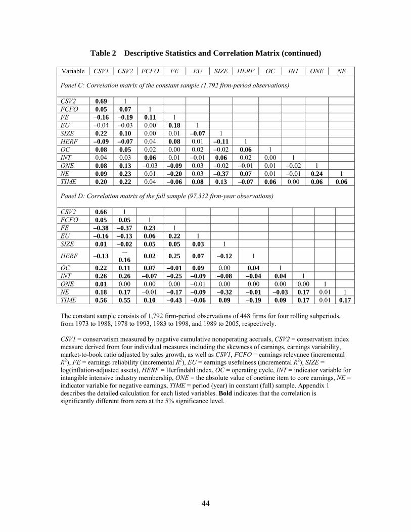
44

Table 2 Descriptive Statistics and Correlation Matrix (continued) Variable CSV1 CSV2 FCFO FE EU SIZE HERF OC INT ONE NE

Panel C: Correlation matrix of the constant sample (1,792 firm-period observations) CSV2 0.69 1 FCFO 0.05 0.07 1 FE –0.16 –0.19 0.11 1 EU –0.04 –0.03 0.00 0.18 1 SIZE 0.22 0.10 0.00 0.01 –0.07 1 HERF –0.09 –0.07 0.04 0.08 0.01 –0.11 1 OC 0.08 0.05 0.02 0.00 0.02 –0.02 0.06 1 INT 0.04 0.03 0.06 0.01 –0.01 0.06 0.02 0.00 1 ONE 0.08 0.13 –0.03 –0.09 0.03 –0.02 –0.01 0.01 –0.02 1 NE 0.09 0.23 0.01 –0.20 0.03 –0.37 0.07 0.01 –0.01 0.24 1 TIME 0.20 0.22 0.04 –0.06 0.08 0.13 –0.07 0.06 0.00 0.06 0.06

Panel D: Correlation matrix of the full sample (97,332 firm-year observations) CSV2 0.66 1 FCFO 0.05 0.05 1 FE –0.38 –0.37 0.23 1 EU –0.16 –0.13 0.06 0.22 1 SIZE 0.01 –0.02 0.05 0.05 0.03 1

HERF –0.13 –-

0.16 0.02 0.25 0.07 –0.12 1

OC 0.22 0.11 0.07 –0.01 0.09 0.00 0.04 1 INT 0.26 0.26 –0.07 –0.25 –0.09 –0.08 –0.04 0.04 1 ONE 0.01 0.00 0.00 0.00 –0.01 0.00 0.00 0.00 0.00 1 NE 0.18 0.17 –0.01 –0.17 –0.09 –0.32 –0.01 –0.03 0.17 0.01 1 TIME 0.56 0.55 0.10 –0.43 –0.06 0.09 –0.19 0.09 0.17 0.01 0.17 The constant sample consists of 1,792 firm-period observations of 448 firms for four rolling subperiods, from 1973 to 1988, 1978 to 1993, 1983 to 1998, and 1989 to 2005, respectively. CSV1 = conservatism measured by negative cumulative nonoperating accruals, CSV2 = conservatism index measure derived from four individual measures including the skewness of earnings, earnings variability, market-to-book ratio adjusted by sales growth, as well as CSV1, FCFO = earnings relevance (incremental R2), FE = earnings reliability (incremental R2), EU = earnings usefulness (incremental R2), SIZE = log(inflation-adjusted assets), HERF = Herfindahl index, OC = operating cycle, INT = indicator variable for intangible intensive industry membership, ONE = the absolute value of onetime item to core earnings, NE = indicator variable for negative earnings, TIME = period (year) in constant (full) sample. Appendix 1 describes the detailed calculation for each listed variables. Bold indicates that the correlation is significantly different from zero at the 5% significance level.

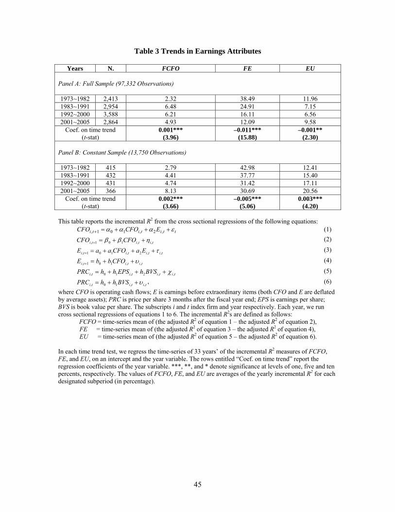
45

Table 3 Trends in Earnings Attributes

Years N. FCFO FE EU Panel A: Full Sample (97,332 Observations) 1973~1982 2,413 2.32 38.49 11.96 1983~1991 2,954 6.48 24.91 7.15 1992~2000 3,588 6.21 16.11 6.56 2001~2005 2,864 4.93 12.09 9.58

Coef. on time trend (t-stat)

0.001*** (3.96)

–0.011*** (15.88)

–0.001** (2.30)

Panel B: Constant Sample (13,750 Observations) 1973~1982 415 2.79 42.98 12.41 1983~1991 432 4.41 37.77 15.40 1992~2000 431 4.74 31.42 17.11 2001~2005 366 8.13 30.69 20.56

Coef. on time trend (t-stat)

0.002*** (3.66)

–0.005*** (5.06)

0.003*** (4.20)

This table reports the incremental R2 from the cross sectional regressions of the following equations:

ttititi ECFOCFO ,2,101, (1)

tititi CFOCFO ,,101, (2)

titititi EaCFOaaE ,,2,101, (3)

tititi CFObbE ,,101, (4)

titititi BVShEPShhPRC ,,2,10, (5)

tititi BVShhPRC ,,10, , (6)

where CFO is operating cash flows; E is earnings before extraordinary items (both CFO and E are deflated by average assets); PRC is price per share 3 months after the fiscal year end; EPS is earnings per share; BVS is book value per share. The subscripts i and t index firm and year respectively. Each year, we run cross sectional regressions of equations 1 to 6. The incremental R2s are defined as follows:

FCFO = time-series mean of (the adjusted R2 of equation 1 – the adjusted R2 of equation 2), FE = time-series mean of (the adjusted R2 of equation 3 – the adjusted R2 of equation 4), EU = time-series mean of (the adjusted R2 of equation 5 – the adjusted R2 of equation 6). In each time trend test, we regress the time-series of 33 years’ of the incremental R2 measures of FCFO, FE, and EU, on an intercept and the year variable. The rows entitled “Coef. on time trend” report the regression coefficients of the year variable. ***, **, and * denote significance at levels of one, five and ten percents, respectively. The values of FCFO, FE, and EU are averages of the yearly incremental R2 for each designated subperiod (in percentage).

46

Table 4 Frequency Analysis of the Trade-off

Panel A: Bivariate Analysis

Current Earnings’ Ability to Predict Future Cash Flows

Current Earnings’ Ability to Predict Future Earnings

Total

Bottom 50% FE Top 50% FE Bottom 50% FCFO

Observed Expected

Observed-Expected Percent

491 448 43

(27%)

405 448 –43

(23%)

896

(50%) Top 50% FCFO

Observed Expected

Observed-Expected Percent

405 448 –43

(23%)

491 448 43

(27%)

896

(50%) Total 896

(50%) 896

(50%) 1792

(100%) Chi-Square: Value Prob.

16.51 <0.0001

Panel B: Conditional on Conservatism (Trade-off Group)

High Conservatism (Top 50%)

Low Conservatism (Bottom 50%)

Trade-Off 1: Top 50% FCFO & Bottom 50% FE

Observed Expected

Observed-Expected Percent

231 194 37

(29%)

174 212 –38

(21%)

405

(50%) Trade-off 2: Top 50% FE &

Bottom 50% FCFO Observed Expected

Observed-Expected Percent

156 194 –38

(19%)

249 212 37

(31%)

405

(50%) Total 387

(48%) 423

(52%) 810

(100%) Chi-Square: Value Prob.

27.83 <0.0001

The frequency analysis is based on the 1,792 firm-period observations of the constant sample. The two off-diagonal cells of panel A are the trade-off cells of the top 50% in FCFO and the bottom 50% in FE, or the bottom 50% in FCFO and the top 50% in FE. Panel B presents frequency tables for firms in the trade-off cells of panel A conditional on high/low accounting conservatism (defined by the median value of CSV2). The expected frequency is calculated as the product of the marginal frequencies for the row and column (row and column totals) of the desired cell, divided by the total number of observations, i.e., Expected Cell Frequency = (Row Total*Column Total)/Total observations. The null hypothesis for the chi-square test is that the rows and columns of the contingency are independent.

47

Table 5 Relevance and Reliability Regressions

Constant Sample Full Sample CSV1 CSV2 CSV1 CSV2

Predicted Sign

Eq. 7 Eq. 8

Equation 7 Relevance

Equation 8 Reliability

Equation 7 Relevance

Equation 8 Reliability

Equation 7 Relevance

Equation 8 Reliability

Equation 7 Relevance

Equation 8 Reliability

Intercept

0.08*** (7.96)

0.25*** (15.10)

0.05** (2.84)

0.40*** (15.27)

0.04*** (4.35)

0.26*** (13.16)

0.04*** (3.78)

0.26*** (13.24)

CSV1

+ – 0.26** (2.31)

–1.20*** (6.96)

0.38* (1.86)

–1.72*** (7.05)

CSV2

+ – 0.03** (2.45)

–0.15*** (8.37)

0.02** (2.27)

–0.07*** (4.27)

SIZE

+ + –0.01 (0.43)

0.004* (1.86)

–0.00 (0.13)

0.00 (1.03)

0.002*** (4.53)

0.003*** (3.61)

0.002*** (5.14)

0.003*** (3.27)

HERF

+ + 0.07** (2.20)

0.18*** (3.14)

0.07** (2.21)

0.18** (3.08)

0.08* (1.85)

0.49*** (5.47)

0.07* (1.80)

0.47*** (5.56)

OC

+ + 0.00 (0.75)

0.00 (0.55)

0.00 (0.82)

0.00 (0.37)

0.00004** (2.51)

0.00009*** (3.14)

0.00005*** (2.74)

0.00 (1.14)

INT

? ? 0.01 (1.39)

0.01 (0.63)

0.01 (1.41)

0.01 (0.58)

–0.01* (1.77)

–0.04*** (4.41)

–0.01 (1.66)

–0.04*** (4.67)

TIME

+ – 0.00 (0.56)

–0.01 (1.26)

0.00 (0.44)

–0.00 (0.83)

Adj. R2

(%) 0.44 3.16 0.50 4.07

N 1,745 1,745 1,745 1,745 33 33 33 33 Equation 7 (the relevance equation) is: ,,6,5,4,3,2,10, jijjijijijijiji TIMEdINTdOCdHERFdSIZEdCSVddFCFO and

equation 8 (the reliability equation) is: ,,6,5,4,3,2,10, jijjijijijijiji TIMEeINTeOCeHERFeSIZEeCSVeeFE where FCFO = earnings relevance

(incremental R2), FE = earnings reliability (incremental R2), CSV = conservatism (CSV1 and CSV2), SIZE = log(inflation-adjusted assets), HERF = Herfindahl index, OC = operating cycle, INT = indicator variable for intangible intensive industries, and TIME = period in constant sample analysis, the subscript i indexes firm, and the subscript j indexes period (year) in constant (full) sample analysis. We run pooled regressions for the constant sample and the Fama-MacBeth yearly cross-sectional regressions for the full sample using the generalized least squares (GLS) method. Equations 7 and 8 are estimated with 1,745 observations from the constant sample resulting from the removal of 47 observations (from the 1,792 original observations) that have missing values for the OC variable or are outliers with absolute value of the r-student statistic greater than 4. Coefficients reported for the full sample are means of the 33 yearly regression coefficients covering the 33-year sample period. Corresponding t statistics also are reported. The average number of observations for each yearly regression is approximately 2,600. The t-statistics are reported in parentheses. ***, **, and * denote significance at levels of 1, 5, and 10%, respectively.

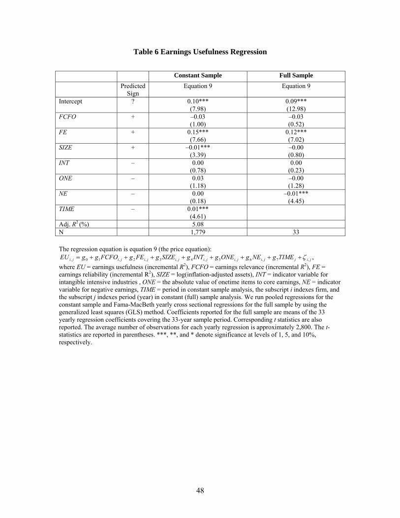
48

Table 6 Earnings Usefulness Regression

Constant Sample Full Sample

Predicted Sign

Equation 9 Equation 9

Intercept

?

0.10*** (7.98)

0.09*** (12.98)

FCFO

+

–0.03 (1.00)

–0.03 (0.52)

FE

+

0.15*** (7.66)

0.12*** (7.02)

SIZE

+

–0.01*** (3.39)

–0.00 (0.80)

INT

–

0.00 (0.78)

0.00 (0.23)

ONE

–

0.03 (1.18)

–0.00 (1.28)

NE

– 0.00 (0.18)

–0.01*** (4.45)

TIME

– 0.01*** (4.61)

Adj. R2 (%) 5.08 N 1,779 33

The regression equation is equation 9 (the price equation):

,,7,6,5,4,3,2,10, jijjijijijijijiji TIMEgNEgONEgINTgSIZEgFEgFCFOggEU

where EU = earnings usefulness (incremental R2), FCFO = earnings relevance (incremental R2), FE = earnings reliability (incremental R2), SIZE = log(inflation-adjusted assets), INT = indicator variable for intangible intensive industries , ONE = the absolute value of onetime items to core earnings, NE = indicator variable for negative earnings, TIME = period in constant sample analysis, the subscript i indexes firm, and the subscript j indexes period (year) in constant (full) sample analysis. We run pooled regressions for the constant sample and Fama-MacBeth yearly cross sectional regressions for the full sample by using the generalized least squares (GLS) method. Coefficients reported for the full sample are means of the 33 yearly regression coefficients covering the 33-year sample period. Corresponding t statistics are also reported. The average number of observations for each yearly regression is approximately 2,800. The t-statistics are reported in parentheses. ***, **, and * denote significance at levels of 1, 5, and 10%, respectively.

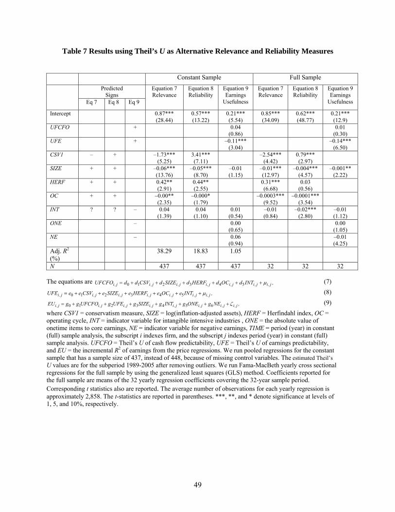
49

Table 7 Results using Theil’s U as Alternative Relevance and Reliability Measures

Constant Sample Full Sample

Predicted Signs

Eq 7 Eq 8 Eq 9

Equation 7 Relevance

Equation 8 Reliability

Equation 9 Earnings

Usefulness

Equation 7 Relevance

Equation 8 Reliability

Equation 9 Earnings

Usefulness

Intercept

0.87*** (28.44)

0.57*** (13.22)

0.21*** (5.54)

0.85*** (34.09)

0.62*** (48.77)

0.21*** (12.9)

UFCFO

+ 0.04 (0.86)

0.01 (0.30)

UFE

+ –0.11*** (3.04)

–0.14*** (6.50)

CSV1

–

+ –1.73*** (5.25)

3.41*** (7.11)

–2.54*** (4.42)

0.79*** (2.97)

SIZE

+

+ –0.06*** (13.76)

–0.05*** (8.70)

–0.01 (1.15)

–0.01*** (12.97)

–0.004*** (4.57)

–0.001** (2.22)

HERF

+

+ 0.42** (2.91)

0.44** (2.55)

0.31*** (6.68)

0.03 (0.56)

OC

+

+ –0.00** (2.35)

–0.000* (1.79)

–0.0003*** (9.52)

–0.0001*** (3.54)

INT

? ? – 0.04 (1.39)

0.04 (1.10)

0.01 (0.54)

–0.01 (0.84)

–0.02*** (2.80)

–0.01 (1.12)

ONE

– 0.00 (0.65)

0.00 (1.05)

NE

– 0.06 (0.94)

–0.01 (4.25)

Adj. R2

(%) 38.29 18.83 1.05

N 437 437 437 32 32 32 The equations are 0 1 2 3 4 5i , j i , j i , j i , j i , j i , j i , jUFCFO d d CSV d SIZE d HERF d OC d INT , (7)

0 1 2 3 4 5i , j i , j i , j i , j i , j i , j i , jUFE e e CSV e SIZE e HERF e OC e INT , (8)

0 1 2 3 4 5 6i , j i , j i , j i , j i , j i , j i , j i , jEU g g UFCFO g UFE g SIZE g INT g ONE g NE , (9)

where CSV1 = conservatism measure, SIZE = log(inflation-adjusted assets), HERF = Herfindahl index, OC = operating cycle, INT = indicator variable for intangible intensive industries , ONE = the absolute value of onetime items to core earnings, NE = indicator variable for negative earnings, TIME = period (year) in constant (full) sample analysis, the subscript i indexes firm, and the subscript j indexes period (year) in constant (full) sample analysis. UFCFO = Theil’s U of cash flow predictability, UFE = Theil’s U of earnings predictability, and EU = the incremental R2 of earnings from the price regressions. We run pooled regressions for the constant sample that has a sample size of 437, instead of 448, because of missing control variables. The estimated Theil’s U values are for the subperiod 1989-2005 after removing outliers. We run Fama-MacBeth yearly cross sectional regressions for the full sample by using the generalized least squares (GLS) method. Coefficients reported for the full sample are means of the 32 yearly regression coefficients covering the 32-year sample period. Corresponding t statistics also are reported. The average number of observations for each yearly regression is approximately 2,858. The t-statistics are reported in parentheses. ***, **, and * denote significance at levels of 1, 5, and 10%, respectively.

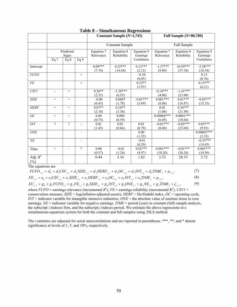
50

Table 8 – Simultaneous Regressions Constant Sample (N=1,745)

Full Sample (N=80,789)

Constant Sample Full Sample

Predicted Signs

Eq 7 Eq 8 Eq 9

Equation 7 Relevance

Equation 8 Reliability

Equation 9 Earnings

Usefulness

Equation 7 Relevance

Equation 8 Reliability

Equation 9 Earnings

Usefulness

Intercept

0.08*** (7.74)

0.25*** (14.64)

0.12*** (2.12)

–1.37*** (9.89)

10.59*** (37.34)

–5.38*** (10.34)

FCFO

+ –0.38 (0.85)

0.15 (0.76)

FE

+ 0.23** (1.97)

0.15*** (6.21)

CSV1

–

+ 0.26** (2.32)

–1.20*** (6.53)

0.14*** (4.08)

–1.41*** (21.00)

SIZE

+

+ –0.00 (0.43)

0.004* (1.78)

–0.01*** (3.69)

0.001*** (8.88)

0.01*** (16.87)

–0.02*** (15.23)

HERF

+

+ 0.07** (2.10)

0.18** (3.30)

0.01 (1.08)

0.34*** (21.49)

OC

+

+ 0.00 (0.75)

0.000 (0.59)

0.00004*** (6.69)

0.0001*** (10.66)

INT

? ? – 0.01 (1.45)

0.01 (0.66)

0.01 (0.79)

–0.01*** (8.60)

–0.05*** (23.69)

0.03*** (9.93)

ONE

– 0.00 (1.52)

0.00003*** (3.33)

NE

– –0.01 (0.20)

–0.33*** (14.65)

Time + – ? 0.00 (0.57)

–0.01 (1.24)

0.02*** (4.97)

0.001*** (10.20)

–0.01*** (36.24)

0.003*** (10.50)

Adj. R2

(%) 0.44 3.16 1.82 2.33 28.33 2.72

The equations are ,,6,5,4,3,2,10, jijjijijijijiji TIMEdINTdOCdHERFdSIZEdCSVddFCFO (7)

,,6,5,4,3,2,10, jijjijijijijiji TIMEeINTeOCeHERFeSIZEeCSVeeFE (8)

,,7,6,5,4,3,2,10, jijjijijijijijiji TIMEgNEgONEgINTgSIZEgFEgFCFOggEU (9) where FCFO = earnings relevance (incremental R2), FE = earnings reliability (incremental R2), CSV1 = conservatism measure, SIZE = log(inflation-adjusted assets), HERF = Herfindahl index, OC = operating cycle, INT = indicator variable for intangible intensive industries, ONE = the absolute value of onetime items to core earnings, NE = indicator variable for negative earnings, TIME = period (year) in constant (full) sample analysis, the subscript i indexes firm, and the subscript j indexes period. We estimate the above regressions in a simultaneous-equations system for both the constant and full samples using 2SLS method. The t-statistics are adjusted for serial autocorrelations and are reported in parentheses. ***, **, and * denote significance at levels of 1, 5, and 10%, respectively.

51

Table 9 Portfolio Analysis

Constant Sample (N = 13,750) Full Sample (N = 97,332)

Panel A: Conditional on Earnings Reliability and Conservatism (∆FE and ∆CSV1): High ∆FE and Low ∆CSV1 versus Low ∆FE and High ∆CSV1

High ∆FE and Low ∆CSV1

Low ∆FE and High ∆CSV1

Difference High ∆FE and Low ∆CSV1

Low ∆FE and High ∆CSV1

Difference

τ1

0.008*** (6.75)

–0.002* (1.96)

0.010*** (6.25)

0.001 (1.48)

–0.002*** (3.77)

0.003*** (3.56)

No. of Obs.

3,500 3,439 24,945 38,575

Percentage of

total obs. #

3,500/13,750 = 25%

3,439/13,750 =25%

24,945/97,332 =26%

38,575/97,332 =40%

Panel B: Conditional on Negative Earnings and Onetime Item (∆NE and ∆ONE): High ∆NE and High ∆ONE versus Low ∆NE and Low ∆ONE

High ∆NE and High ∆ONE

Low ∆NE and Low ∆ONE

Difference High ∆NE and High ∆ONE

Low ∆NE and Low ∆ONE

Difference

τ1

–0.001 (1.63)

0.005*** (3.99)

–0.006*** (4.27)

–0.002*** (3.83)

0.002*** (3.43)

–0.004*** (5.14)

No. of Obs.

2,668 5,582 46,559 19,439

Percentage of

total obs. #

2,668/13,750 = 19%

5,582/13,750 =41%

46,559/97,332 =48%

19,439/97,332 =20%

We first sort firms into portfolios using median values of firm characteristics as breakpoints (high = above median and low = below median). For each portfolio, we then derive the cross-sectional estimates of earnings usefulness (EU, or incremental R2), and run the regression

ttt YEAREU *10, where YEAR is

the year variable for the 33 years of the sample period from 1973 to 2005. The firm characteristics are the change in earnings reliability (∆FE), the change in conservatism (∆CSV1), the change in onetime items (∆ONE), and/or the change in the frequency of negative earnings (∆NE). For the constant sample, each firm’s ∆FE = 1989–2005 subperiod FE minus 1973–1989 subperiod FE. For the full sample, we first group firms by industry. We then calculate the average of ∆FE (current year FE – previous year FE) for each industry, and apply the median value of the 41 industry averages as the breakpoint for the 41 industries (and firms therein). Breakpoints for other variables are analogously defined. The “Difference” columns report the statistics for the test of the equality of the time coefficients (τ 1) of the two portfolios being compared. The t-statistics are reported in parentheses. ***, **, and * denote significance at levels of 1, 5, and 10%, respectively.

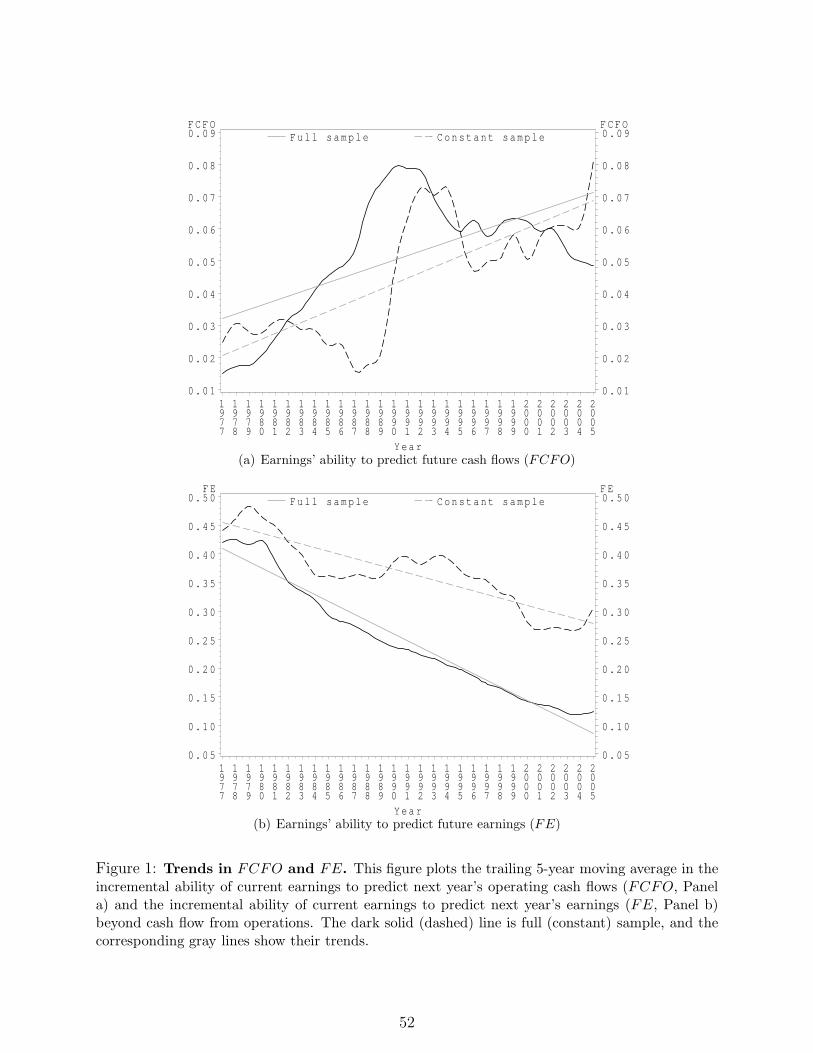
Full sample Constant sampleFCFO

0.01

0.02

0.03

0.04

0.05

0.06

0.07

0.08

0.09

Year

1977

1978

1979

1980

1981

1982

1983

1984

1985

1986

1987

1988

1989

1990

1991

1992

1993

1994

1995

1996

1997

1998

1999

2000

2001

2002

2003

2004

2005

FCFO

0.01

0.02

0.03

0.04

0.05

0.06

0.07

0.08

0.09

(a) Earnings’ ability to predict future cash flows (FCFO)

Full sample Constant sampleFE

0.05

0.10

0.15

0.20

0.25

0.30

0.35

0.40

0.45

0.50

Year

1977

1978

1979

1980

1981

1982

1983

1984

1985

1986

1987

1988

1989

1990

1991

1992

1993

1994

1995

1996

1997

1998

1999

2000

2001

2002

2003

2004

2005

FE

0.05

0.10

0.15

0.20

0.25

0.30

0.35

0.40

0.45

0.50

(b) Earnings’ ability to predict future earnings (FE)

Figure 1: Trends in FCFO and FE. This figure plots the trailing 5-year moving average in theincremental ability of current earnings to predict next year’s operating cash flows (FCFO, Panela) and the incremental ability of current earnings to predict next year’s earnings (FE, Panel b)beyond cash flow from operations. The dark solid (dashed) line is full (constant) sample, and thecorresponding gray lines show their trends.

52

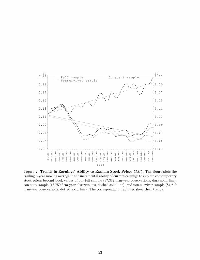
Full sample Constant sampleNonsurvivor sample

EU

0.03

0.05

0.07

0.09

0.11

0.13

0.15

0.17

0.19

0.21

Year

1977

1978

1979

1980

1981

1982

1983

1984

1985

1986

1987

1988

1989

1990

1991

1992

1993

1994

1995

1996

1997

1998

1999

2000

2001

2002

2003

2004

2005

EU

0.03

0.05

0.07

0.09

0.11

0.13

0.15

0.17

0.19

0.21

Figure 2: Trends in Earnings’ Ability to Explain Stock Prices (EU). This figure plots thetrailing 5-year moving average in the incremental ability of current earnings to explain contemporarystock prices beyond book values of our full sample (97,332 firm-year observations, dark solid line),constant sample (13,750 firm-year observations, dashed solid line), and non-survivor sample (84,219firm-year observations, dotted solid line). The corresponding gray lines show their trends.

53

Full sample Constant sampleCSV2

0.2

0.7

1.2

1.7

2.2

2.7

3.2

3.7

Year

1977

1978

1979

1980

1981

1982

1983

1984

1985

1986

1987

1988

1989

1990

1991

1992

1993

1994

1995

1996

1997

1998

1999

2000

2001

2002

2003

2004

2005

CSV2

0.2

0.7

1.2

1.7

2.2

2.7

3.2

3.7

Figure 3: Trends in Accounting Conservatism (CSV 2). This figure plots the trailing 5-yearmoving average in CSV 2 (the conservatism index) of our full sample (dark solid line) and constantsample (dashed solid line). The corresponding gray lines show their trends.

54