Accepted to Nanotechnology - arXiv

1

Accepted to Nanotechnology

The Band Excitation Method in Scanning Probe Microscopy for

Rapid Mapping of Energy Dissipation on the Nanoscale

Stephen Jesse,1 Sergei V. Kalinin,1,2,* Roger Proksch,3 A.P. Baddorf,1,2 and B.J. Rodriguez1,2

1 Materials Science and Technology Division, Oak Ridge National Laboratory,

Oak Ridge, TN 37831

2 Center for Nanophase Materials Sciences, Oak Ridge National Laboratory,

Oak Ridge, TN 37831

3 Asylum Research, 6310 Hollister Ave., Santa Barbara, CA 93117

Abstract

Mapping energy transformation pathways and dissipation on the nanoscale and

understanding the role of local structure on dissipative behavior is a grand challenge for

imaging in areas ranging from electronics and information technologies to efficient energy

production. Here we develop a novel Scanning Probe Microscopy (SPM) technique in which

the cantilever is excited and the response is recorded over a band of frequencies

simultaneously rather than at a single frequency as in conventional SPMs. This band

excitation (BE) SPM allows very rapid acquisition of the full frequency response at each point

* Corresponding author, [email protected]

2

(i.e. transfer function) in an image and in particular enables the direct measurement of energy

dissipation through the determination of the Q-factor of the cantilever-sample system. The BE

method is demonstrated for force-distance and voltage spectroscopies and for magnetic

dissipation imaging with sensitivity close to the thermomechanical limit. The applicability of

BE for various SPMs is analyzed, and the method is expected to be universally applicable to

all ambient and liquid SPMs.

3

I. Introduction

Energy transformations and the inevitable dissipation associated with it are integral

components of the physical world. Development of the science of energy dissipation at its

fundamental length scales will have enormous implications on such varied technologies as

energy production and utilization1 and in nanoscale electronic applications and information

technologies.2 Often, macroscopic dissipation has its origin in disperse, highly localized, low-

dimensional centers. For instance, transport properties in metals and semiconductors are

controlled by scattering at impurities, energy losses in magnetization reversal processes are

determined by magnetoacoustic phonon generation associated with domain wall motion and

depinning, and energy losses during viscoelastic processes are related to crystal defect

motion. Understanding of atomistic dissipation mechanisms and improved engineering of

materials and device strategies to minimize energy losses necessitate the development of

techniques capable of imaging and characterizing nanoscale dissipative processes on the level

of a single dislocation, structural defect, or dopant atom.

Dissipation in materials and devices on the macroscopic scale is easily accessible

through direct measurements. The area of the hysteresis loop in ferroelectric or magnetic

measurements provides a measure of irreversible work in the system. Similarly, dissipated

power can be determined from current-voltage measurements for electric dissipation and loss

modulus measurements for mechanical dissipation. Finally, heat generation in a system can be

measured to provide information on dissipated energy. However, these macroscale

measurements of collective phenomena are not easily extendable to the nanoscale.

Here, we introduce a novel excitation and measurement mode (band excitation, or BE)

that allows rapid mapping of energy dissipation on the nanoscale. BE utilizes a non-sinusoidal

4

excitation signal having a finite amplitude over a selected band in frequency space that

substitutes the sinusoidal excitation in standard Scanning Probe Microscopies. The principles

of energy dissipation measurement and the limitations of classical SPM detection modes are

discussed in Section II. The principles of band excitation and experimental implementation of

BE are summarized in Sections III and IV respectively. The BE force-distance and voltage

spectroscopies are presented in Section V, and BE Magnetic Dissipation Force Microscopy is

illustrated in Section VI. The applicability and limitations of the BE method for existing SPM

modes are discussed in Section VII.

II. Energy Dissipation Measurements in SPM

Scanning probe microscopy (SPM), well established for the measurement of

topography and forces on the nanoscale, provides a potential strategy for local dissipation

measurement.3,4,5 In this, the SPM tip concentrates the probing field to the nanometer level,

and the cantilever acts as an energy dissipation sensor. The energy dissipated due to tip-

surface interactions is determined using power balance as 0PPP drivediss −= , where driveP is the

power provided to the probe by an external driving source, and 0P is the sum of intrinsic

losses due to cantilever damping by the surroundings and within the cantilever material. The

external power can be determined from the cantilever dynamics as zFPdrive &= , where F is

the force acting on the probe, z& is the experimentally measured probe velocity, with the

average taken along the probe tip trajectory. The intrinsic losses within the material and due

to the hydrodynamic damping by ambient, 0P , are determined by calibration at a reference

position, 0=dissP .

5

The dynamic behavior of the cantilever weakly interacting with the surface in the

vicinity of the resonance can be well approximated by a simple harmonic oscillator (SHO)

model described by three independent parameters, namely resonant frequency, 0ω , amplitude

at the resonance, 0A , and quality factor, Q , as

( )( ) ( )2222

2max

Q

AA

oo

o

ωωωω

ωω

+−= and ( )( ) 22

tano

o Qωω

ωωωϕ

−= (1a,b)

From these, 0ω is related to the tip-surface force gradient, 0A to the driving force, and

Q to the energy dissipation.6

For constant frequency operation, seminal work by Cleveland et al.7 and Garcia8 has

related energy loss to the phase shift of a vibrating cantilever. Dissipative tip-surface

interactions can be probed via measurement of the amplitude, A , and phase, ϕ , of the

cantilever driven mechanically with amplitude, dA , at a constant frequency, ω , as,

⎥⎦

⎤⎢⎣

⎡−=

0

0

0

2 sin21

ωωϕω

AAQ

QkAP d

tip (2)

where 0ω is the resonance frequency of the cantilever with spring constant, k , and the quality

factor in free space, 0Q .

The emergence of frequency tracking techniques9 provides another means to

determine dissipation. In this, the cantilever is driven at constant amplitude near the resonance

frequency, the response amplitude is measured, and by assuming that changes in the signal

strength are proportional to the Q-factor, dissipation in the system can be ascertained. In this

case,

⎥⎦

⎤⎢⎣

⎡−=

QQkAPtip

1121

00

2ω (3)

6

and Q is the quality factor in the vicinity of the surface. Experimentally, Q is determined

using an additional feedback loop that maintains the oscillation amplitude constant by

adjusting the driving amplitude, dAAQ = . These approaches were implemented by several

groups to study magnetic dissipation,10,11 electrical dissipation,12,13 and mechanical dissipation

on atomic14,15 and molecular levels.16

Notably, in a standard single-frequency SPM experiment the number of independent

parameters defining the cantilever dynamics (i.e. 3 SHO parameters) exceeds the number of

experimentally observed variables (e.g., amplitude and phase), precluding direct measurement

of dissipation. For acoustically driven systems, the constant driving force, constF = ,

provides an additional constraint required to determine 3 independent SHO parameters from

two experimentally accessible quantities [Fig. 1 (a)]. However, Eqs. (2, 3) are no longer valid

for techniques where the driving signal is position, time, or frequency dependent, constF ≠ .

For example, in Kelvin probe force microscopy (KPFM), the driving force, i.e., the capacitive

tip-surface interaction, is proportional to both the local work function and the periodic voltage

applied to the tip. Hence, variations in the signal strength are due both to work function

variations and dissipation, and these effects cannot be separated unambiguously [Fig. 1 (b)].

Similarly, in atomic force acoustic microscopy and piezoresponse force microscopy, which

are used to address local mechanical and electromechanical properties, variations in the local

response cannot be unambiguously distinguished from dissipation.

Even in techniques utilizing constant excitation signals, non-linearities in the tip-

surface interaction result in the creation of higher-harmonics which can cause confusion

between information about dissipation and other properties.17 Furtermore, dissipation

measurements are extremely sensitive to SPM electronics. For example, small deviations in

7

the phase set-point from the resonance condition in frequency tracking techniques result in

major errors in the measured dissipation energy. Most importantly, implementation of these

techniques requires the calibration of the frequency response of the piezoactuator driving the

cantilever.18 In the absence of such calibration, the images often demonstrate abnormal

cantilever-dependent contrast. All together, these factors contribute to a relative paucity of

studies on dissipation processes in SPM.

This limited applicability of SPM to dissipation measurements is a direct consequence

of the fact that traditional SPM excites and samples the response at a single frequency at a

time. This allows fast imaging and high signal levels, but information about the frequency-

dependent response, and hence dissipation and energy transfer, is not probed. At the other

extreme, spectroscopic techniques excite and sample over all Fourier space (up to the

bandwidth limit of the electronics), but the response amplitude is necessarily small since the

excitation energy is spread over all frequencies.19 Finally, response in the vicinity of the

resonance can be probed using frequency sweeps. However in this case, homodyne detection

implemented in standard lock-in techniques results in significant phase and amplitude errors

and information loss if the relaxation time of the oscillator exceeds the residence time at each

frequency. This necessitates long acquisition times to achieve adequate signal to noise ratios,

incompatible with 1-30 ms/pixel data acquisition times required for practical SPM imaging.

III. Principles of Band Excitation Method

Here, we develop and implement a method based on an adaptive, digitally synthesized

signal that excites and detects within a band of frequencies over a selected frequency range

simultaneously.20 This approach takes advantage of the fact that only selected regions of

8

Fourier space contain information of any practical interest, for instance in the vicinity of

resonances. Instead of a simple sinusoidal excitation, the BE method developed here uses a

signal having a predefined amplitude and phase content. The generic process is illustrated in

Fig. 2. The signal is generated to have the predefined Fourier amplitude density in the

frequency band of interest and inverse Fourier transformed to generate excitation signal in

time domain. Resulting complex waveform is used to excite the cantilever electrically,

acoustically, or magnetically. The cantilever response to the BE drive is measured and Fourier

transformed to yield the amplitude- and phase-frequency curves and is stored at each point in

the image as a 3D [ ( )ωA and ( )ωθ at each point] data sets. The ratio of the response and

excitation signals yields the transfer function of the system.

The applicability of BE is analyzed as following. The point spacing in the frequency

domain is Tf 1=Δ , where T is the pulse duration (equal to pixel time, ~20 ms for 0.4 Hz

scan rate at 128 points/pixel). For a resonance frequency of 0ω = 150 kHz and Q-factor of ~

200, the width of the resonance peak is ~750 Hz, allowing for sufficient sampling of the peak

in the frequency domain (15 points above the half-max). The sampling efficiency increases

for lower Q-factors (e.g., imaging in liquids) and higher resonance frequencies (contact modes

and stiff cantilevers). Remarkably, the parallel detection of the BE method implies that the

total number of frequency points (i.e., the width of the band in the Fourier space) can be

arbitrary large, with the cost being the signal/noise ratio. Typically for a single peak tracking,

the frequency band is chosen such that the intensity factor, defined as

( ) ωωω Δ= ∫ maxdet AdAI , where the integral is taken over the frequency band of width ωΔ , is

detI ~ 0.2-0.7. Alternatively, the excitation signal can be tailored to provide a higher excitation

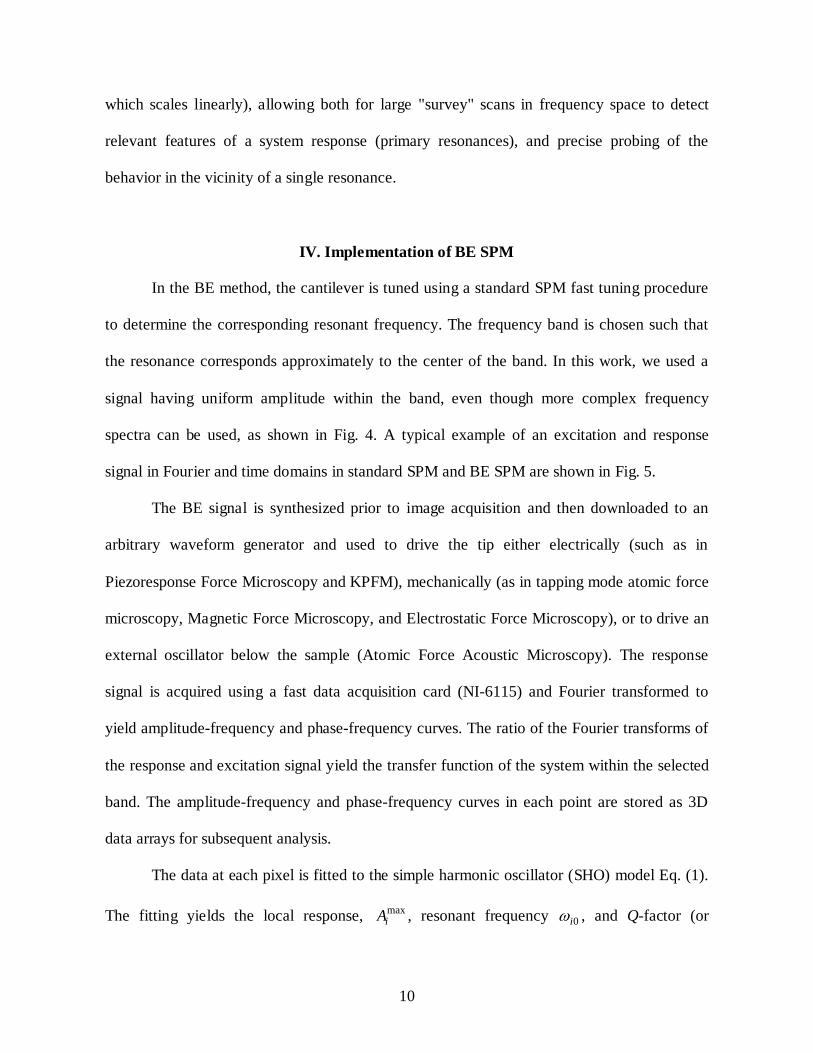
level away from the resonance or to track multiple bands [Fig. 4].

9

The measured response curves can be analyzed in a variety of ways. The most

straightforward is to individually fit each to the simple harmonic oscillator model [Eq. (1)] to

determine the resonant frequency, amplitude, and Q-factor at each point and display each as

2D images and/or use as a feedback signals. This fast Fourier transform/fitting routine

substitutes the traditional lock-in/low-pass filter that provides amplitude and phase at a single

frequency. In the BE method, parallel acquisition of the response at all frequencies within the

band allows complete spectral acquisition at ~10 msec/pixel rate, well within the limit for

SPM imaging. Thus, in the BE response the system is excited and the response is measured

simultaneously at all frequencies within the excited band (parallel detection), maximizing the

signal/noise ratio.

This feature of BE is most obvious in comparison with the lock-in detection. For lock-

in homodyne detection, the optimal sampling of the system response can be achieved only if

the residence time at each frequency point is ωδτ Q> (Fig. 3). Therefore, sampling of the

full amplitude-frequency curve requires a time of ωNQ , where N is number of frequency

points. For N = 100, Q = 500 (typical for ambient non-contact modes), and πω 2= 100 kHz,

this yields a minimum time for a lock-in of ~80 ms/pixel. Most lock-in amplifiers have

additional time constants associated with input and output filters, which can add 0.5 – 5

ms/frequency point, equivalent to ~ 100 ms/pixel. This translates to acquisition times of ~ 4

hours for standard 256x256 image. Hence, compared to standard lock-in detection, the BE

approach allows a time reduction for acquiring a sweep by a factor of 10 to 100 per pixel by

avoiding the requirement for the ωQ delay (or, rather, by performing this detection on all

frequencies in parallel). Notably, the BE acquisition time does not depend on the width of the

frequency band, or, equivalently, the number of frequency points (unlike lock-in detection,

10

which scales linearly), allowing both for large "survey" scans in frequency space to detect

relevant features of a system response (primary resonances), and precise probing of the

behavior in the vicinity of a single resonance.

IV. Implementation of BE SPM

In the BE method, the cantilever is tuned using a standard SPM fast tuning procedure

to determine the corresponding resonant frequency. The frequency band is chosen such that

the resonance corresponds approximately to the center of the band. In this work, we used a

signal having uniform amplitude within the band, even though more complex frequency

spectra can be used, as shown in Fig. 4. A typical example of an excitation and response

signal in Fourier and time domains in standard SPM and BE SPM are shown in Fig. 5.

The BE signal is synthesized prior to image acquisition and then downloaded to an

arbitrary waveform generator and used to drive the tip either electrically (such as in

Piezoresponse Force Microscopy and KPFM), mechanically (as in tapping mode atomic force

microscopy, Magnetic Force Microscopy, and Electrostatic Force Microscopy), or to drive an

external oscillator below the sample (Atomic Force Acoustic Microscopy). The response

signal is acquired using a fast data acquisition card (NI-6115) and Fourier transformed to

yield amplitude-frequency and phase-frequency curves. The ratio of the Fourier transforms of

the response and excitation signal yield the transfer function of the system within the selected

band. The amplitude-frequency and phase-frequency curves in each point are stored as 3D

data arrays for subsequent analysis.

The data at each pixel is fitted to the simple harmonic oscillator (SHO) model Eq. (1).

The fitting yields the local response, maxiA , resonant frequency 0iω , and Q-factor (or

11

dissipation). The fitting can be performed either on amplitude or phase data, or

simultaneously on both. To ensure adequate weighting, in the latter case the data is

transformed into real and imaginary parts, ϕcosA and ϕsinA . The derived SHO coefficients

are plotted as 2D maps. Note that more complex forms of data analysis [using different

physical models,21 statistical fits, wavelet signal transforms,22 etc.] are possible.

The BE method for a single point can then be extended to spectroscopy and imaging in

the point-by-point, and line-by-line modes. In spectroscopic BE measurements, the

waveforms are applied to the probe and the response is measured as a function of a slowly

varying external parameter (tip-surface separation, force, or bias) at a single point of the

surface to yield 2D spectroscopic response-frequency-parameter maps (spectrograms).

Subsequent fitting using SHO model allows 1D response-parameter spectra (e.g., dissipation-

distance or response-distance curves) to be extracted and compared with the varying

parameter (such as force-distance data).

In point-by-point measurements, the tip approaches the surface vertically until the

deflection set-point is achieved. The amplitude-frequency data is then acquired at each point.

After acquisition, the tip is moved to the next location. This is continued until a mesh of

evenly spaced M x N points is scanned to yields 3D data array. Subsequent analysis yields 2D

maps of corresponding quantities.

In line-by-line measurements, the BE signal substitutes the standard driving signal

during the interleave line on a commercial SPM (MultiMode NS-IIIA). The topographic

information in the main line is collected using standard intermittent contact or contact mode

detection. The data is processed using an external data acquisition system and is synchronized

with the SPM topographic image to yield BE maps.

12

V. Force-Distance and Voltage Spectroscopy with BE-SPM

In the following, we illustrate the applicability of the BE method to several specific

SPM applications including (i) point force- spectroscopy, (ii) bias- spectroscopy, and (iii)

imaging of magnetic dissipation. As an illustration of point force spectroscopy, BE-mapping

of the frequency dependence of the cantilever response with tip-surface separation under an

electrostatic driving force is illustrated in Fig. 6 (a). The measurements are performed on

freshly cleaved mica surface in ambient using gold-coated tips (Micromasch, k = 1 N/m). On

approaching the surface (bottom to top) the response gradually increases due to an increase of

capacitive forces, while the resonance frequency remains constant (Region I). In close vicinity

to the surface, the resonant frequency decreases due to strong attractive interactions (inset). A

rapid change in the resonant structure occurs upon transition from the free to bound cantilever

modes (jump to contact). Upon increasing the contact force by loading the cantilever, a slight

increase in contact stiffness is observed (Region II). The reverse sequence is observed during

retraction (Region III). The total acquisition time for this data is 100 s. The individual

resonances at points along the vertical tip trajectory can be fitted by the SHO model and the

resulting evolution of amplitude, resonant frequency, and dissipation are shown in Fig. 6 (b).

These data illustrate BE spectroscopy of the dissipation in the near-surface layer and bulk

material.23 In these cases, the increased damping for small interaction forces is due to the

relatively larger contribution of the surface layer to the overall contact. Note that BE allows

the probing of extremely broad frequency range (25 – 250 kHz) in ~ 1 s – a comparable scan

using lock-in at single frequency would require ~30 min.

13

A second example of the BE method is the voltage spectroscopy of dynamic processes

in ferroelectric materials. Here, the dynamic response of the electrically driven, conductive

cantilever in contact with a ferroelectric LiNbO3 surface is measured as a function of dc bias

on the tip, as illustrated in Fig. 7 (a), with a total acquisition time of 100 s. The response

amplitude, resonance frequency, and quality factor are shown in Fig. 7 (b). The rapid decrease

in amplitude and quality factor outside the -50 V < Vdc < 50 V interval is associated with the

nucleation of ferroelectric domains and the opening of additional damping channels due to the

motion of the newly formed ferroelectric domain walls. The formation of a domain can be

observed in the standard PFM image after data acquisition [inset in Fig. 7 (a)] (note that

experiment was performed twice, giving rise to two domains).

VI. Imaging Magnetic Dissipation with BE-MFM

The BE method is universally applicable for SPM provided that sufficient sampling of

the resonance curve can be achieved for point spacing in frequency domain Tf 1=Δ , where

T is the pulse duration (time per pixel). At the same time, an arbitrarily broad frequency band

can be excited, at the expense of the signal to noise ratio. Practically, these considerations

favor the BE method for the systems with high resonance frequencies and moderate Q-factors

(10-100), corresponding to the resonant peak width > ~0.3 kHz. Experimentally, most contact

mode techniques have high resonant frequency (the first contact mode resonance is ~ 4 times

the free resonance) and lower Q-factors. Similarly, imaging in liquid is typically associated

with low Q-factors (~1-20, as compared to 100-600 in air). Hence, to demonstrate the

universal applicability of the BE method for ambient and liquid SPMs, we have chosen

14

Magnetic Force Microscopy (MFM) as a prototype model with relatively low resonance

frequency (~50-100 kHz) and high quality factors (typically ~200).

BE-MFM was implemented in a standard line-by-line interleave mode with

intermittent contact mode feedback for topographic detection. As a model system for

magnetic dissipation measurements, we have chosen Yttrium- Iron garnet (YIG, Y3Fe5O12),

dissipation in which have been studied previously by conventional Magnetic Dissipation

Force Microscopy,11 i.e. phase detection in MFM using Cleveland method for analysis of

phase data. A large scale MFM image is shown in Fig. 8. The images exhibit a “flower-like”

magnetic domain pattern characteristic for this material. Superimposed on the pattern are

small circular features corresponding to dissipation at the defect centers in YIG.24 The MDFM

images obtained with standard sinusoidal driving11 in all cases show the superposition of

domain and dissipative contrasts. As discussed above, this is a consequence of the detection

mechanism in which changes in Q-factor cannot be probed reliably without calibration of the

probe transfer function.18

In BE-MFM, the standard, sinusoidal excitation and phase-locked loop frequency

detection is substituted for direct acquisition of the response in the predefined frequency

interval. Shown in Fig. 9 (a-d) are the surface topography, amplitude, quality factor, and

resonance frequency BE MFM images of the YIG surface. Note that the amplitude image

shows only weak variation across the surface, as expected. The frequency shift image shows

flower-like patterns with high contrast, similar to standard MFM with frequency tracking. The

Q-factor image illustrates the characteristic circular features due to magnetic dissipation.

The dissipation power at the defect compared to the sample surface can be estimated

as ≈Δ= 20

2 2QQkAPtip ω 0.012 pW. In this estimate, the effective amplitude is scaled by

15

the intensity factor, detI , taking into account the response decay away from the resonance.

Experimental noise in the Q-factor image is 0.8. The theoretical thermal limit is

0232 2 ωδ kABTQkQ B= , where Bk is Boltzmann’s constant and B is the measurement

bandwidth.10 For our case ( k = 2.55 N/m, A = 9 nm, 0ω = 75 kHz, Q = 199) the

thermomechanical limit on dissipation sensitivity is Qδ = 0.14 for a bandwidth of 33 Hz.

Hence, the BE method allows dissipation detection with sensitivity close to the

thermomechanical noise of the cantilever.

Note that unlike conventional MFM, the amplitude, resonant frequency, and

dissipation are measured independently, thus achieving independent determination of the

three SHO parameters. Furthermore, this approach can be extended to most ambient and

liquid SPM techniques, including electrical imaging by Kelvin probe force microscopy

(KPFM) and electrostatic force microscopy (EFM), acoustic imaging by AFAM, and

electromechanical imaging by PFM.

VII. Summary

To summarize, we have developed an approach for dissipation imaging and transfer

function determination in SPM based on a digitally synthesized excitation signal having a

finite amplitude density in a predefined frequency range. This approach allows direct probing

of the Q-factor of the cantilever, avoiding the limitations of standard lock-in detection. The

applicability of the BE approach is demonstrated for mapping energy dissipation in MFM,

mechanical and electromechanical probes, including loss processes during ferroelectric

domain formation, and the evolution of dynamic behavior of the probes during force-distance

curve acquisition. These examples illustrate the universality of the BE method, which can be

16

used as an excitation and control method in all ambient and liquid SPM methods, including

standard intermittent mode topographic imaging, magnetic imaging by MFM, electrical

imaging by KPFM and EFM, acoustic imaging by AFAM, and electromechanical imaging by

PFM. In these techniques, BE allows direct measurement of previously unavailable

information of energy dissipation in magnetic, electrical, and electromechnical processes.

The capability of mapping local energy dissipation on the nanoscale is an enabling

technology that will open a pathway towards atomistic mechanism of dissipation and establish

relationships between dissipation and structure. This, in turn, will eventually allow the

development of strategies to minimize and avoid undesirable energy losses in technologies as

diverse as electronics, information technology, and energy storage, transport, and generation.

Furthermore, energy dissipation measurements will open a window into energy

transformation mechanisms during fundamental physical and chemical processes. Simple

estimates suggest that at room temperature the estimated detection limit in BE method as

limited by thermomechanical noise is QBTkAkP Btip 022 ω= , corresponding to ~ 0.5 fW, or ~31

mV/oscillation level for ambient environment (as compared to currently demonstrated 20

fW).11 At low temperatures or in a high-Q environment, detection of single optical phonon

generation in the tip-surface junction is possible, providing information on the dissipative

processes with broad applicability to nanomechanics and nanotribology. The implementation

of BE method at low temperatures holds the promise of an even further increase of sensitivity

to the level that a single quasiparticle can be detected, providing insight into the fundamental

physics of strongly correlated oxide materials and other systems on the forefront of research.

17

VIII. Acknowledgements

Research sponsored by ORNL SEED funding (SJ and SVK) and in part (BJR, APB)

by the Division of Materials Sciences and Engineering and Office of Basic Energy Sciences,

U.S. Department of Energy, under contract DE-AC05-00OR22725 at Oak Ridge National

Laboratory, managed and operated by UT-Battelle, LLC. The band excitation method is

available as a part of the user program at the Center for Nanophase Materials Science, Oak

Ridge National Laboratory (contact – SVK).

18

Figure Captions

Fig. 1. Single frequency measurements (red dots) are not always adequate for determining Q.

(a) For a constant driving force, the amplitude (peak height) is inversely proportional to the

quality factor (peak width) of the system. In such a case, dissipation can be determined from

amplitude at a single frequency (e.g. at the resonance). (b) For a non-constant driving force

however, the amplitude and dissipation are independent. Hence, probing energy dissipation

requires measuring the response over a range of frequencies across a resonance.

Fig. 2. Operational principle of the BE method in SPM. The excitation signal is digitally

synthesized to have a predefined amplitude and phase in the given frequency window. The

cantilever response is detected and Fourier transformed at each pixel in an image. The ratio of

the FFTs of response and excitation signals yield the cantilever response (transfer function).

Fitting the response to the simple harmonic oscillator yields amplitude, resonance frequency,

and Q-factor that are plotted to yield 2D images, or used as feedback signals.

Fig. 3. Lock-in sweep detection. (a) One type of excitation signal (chirp) can be represented

as (b) a sinusoidal excitation with linearly varying frequency. (c) Standard lock-in probes

operate at a single frequency and can be represented as a band pass filter of width τ1~fΔ .

Hence, the lock-in sweep works as a moving bandpass filter. BE detects the response at all

frequencies simultaneously. (d) Envelope of the response at a given frequency. The linearity

implies that the system responds at the same frequency as the excitation signal. However, due

to the finite quality factor, response is not instant and response amplitude increases from 0 to

19

the saturated value in a time on the order of 0ωQ . Similarly, response persists after initial

excitation. Even in the ideal case (perfect notch filter) lock-in detection loses information in

the shaded region (response after excitation is turned off). The BE method utilizes the full

frequency domain of the excitation, avoiding this dynamic effect. Note that the two methods

are equivalent for low-Q systems.

Fig. 4. Frequency spectrum of excitation signal in single frequency (a) static and (b)

frequency-tracking cases. In frequency tracking methods, the excitation frequency and

excitation amplitude are varied from point to point. In the band excitation method, the

response in the selected frequency window around the resonance is excited. The excitation

signal can have (c) uniform spectral density [as is the case in this paper], or (d) increased

spectral density on the tails of resonance peak to achieve better sampling away from the peak.

(e) The resonance can be excited simultaneously over several resonance windows. Also, (f)

the phase content of the signal can be controlled, for example, to achieve Q-control

amplification. The excitation signal can be selected prior to imaging, or adapted at each point

so that the center of the excitation window follows the resonance frequency (c) or phase

content is updated (f). This is important for e.g. contact mode techniques, when the tip-surface

contact area and hence the resonance frequency changes significantly with position.

Fig. 5. Excitation (blue) and response (red) signals in standard SPM techniques in (a) time

domain and (b) Fourier domain. Excitation (blue) and response (red) signals in BE SPM in (c)

time domain and (d) Fourier domain. In BE, the system response is probed in the specified

20

frequency range (e.g., encompassing a resonance), as opposed to a single frequency in

conventional SPMs.

Fig. 6. (a) Evolution of the dynamic properties of the cantilever-surface system during force-

distance curve acquisition. (b) Deconvolution of the BE data in amplitude, resonant

frequency, and Q-factor measured along the force-distance curve.

Fig. 7. (a) Bias dependence of the amplitude-frequency response curve for the tip in contact

with a ferroelectric LiNbO3 surface. The inset shows the domain formed by the end of the BE

measurement. (b) Bias dependence of amplitude, resonant frequency, and Q-factor. The

saturation of electromechanical response and decrease in Q-factor evidence the onset of

ferroelectric switching, which opens an additional channel for energy dissipation.

Fig. 8. Standard magnetic force microscopy (a) amplitude and (b) phase images of the YIG

surface. The amplitude image shows clear “flower-like” pattern related to the presence of

magnetic domains. Phase image shows rings due to the dissipation energy losses at the

magnetic dissipation centers. Note that both images illustrate both domain-related and

dissipation-related features due to cross-talk.

Fig. 9. (a) Surface topography, (b) response amplitude, (c) resonance frequency, and (d) Q-

factor image of YIG surface obtained in BE MFM. The ring-like structures form due to

magnetic dissipation centers as corroborated by conventional MDFM. The frequency and Q-

factor images illustrate complete decoupling between the force gradient (frequency shift) and

21

dissipation (Q-factor) data. (c) Average amplitude curve, local amplitude curve and difference

between the two at point 1, note the asymmetry. (d) Average amplitude curve, local amplitude

curve and difference between the two at point 2, note the drop in amplitude. Vertical scale for

(a) is 2 nm.

22

Figure 1. Stephen Jesse, Sergei V. Kalinin et al.

23


24

Time

Time A

mpl

itude

Fr

eque

ncy

Time

Res

pons

e

Lock-in detection

Band excitation detection

Lock-in sweep (a)

(b)

(d)

(c)

QtoeAA ω−=

fδ

Band excitation


25


26


27


Region I

Region II

Region III

28


29


30


31

References

1 E.g. http://epa.gov/climatechange/index.html and http://www.climatehotmap.org/

2 International Technology Roadmap for Semiconductors, www.itrs.net/

3 For review, see R. García and R. Pérez, Surf. Sci. Reports 47, 197 (2002).

4 J. Tamayo and R. Garcia, Appl. Phys. Lett. 73, 2926 (1998).

5 A. San Paulo and R. Garcia, Phys. Rev. B 64, 193411 (2001).

6 W.A. Ducker and R.F. Cook, Appl. Phys. Lett. 56, 2408 (1990), also W.A. Ducker, R.F.

Cook, and D.R. Clarke, J. Appl. Phys. 67, 4045 (1990).

7 J.P. Cleveland, B. Anczykowski, A.E. Schmid, and V.B. Elings, Appl. Phys. Lett. 72, 2613

(1998).

8 J. Tamayo and R. Garcia, Appl. Phys. Lett. 73, 2926 (1998).

9 T. R. Albrecht, P. Grütter, D. Horne, and D. Rugar, J. Appl. Phys. 69, 668 (1991).

10 P. Grütter, Y. Liu, P. LeBlanc, and U. Dürig, Appl. Phys. Lett. 71, 279 (1997).

11 R. Proksch, K. Babcock, and J. Cleveland, Appl. Phys. Lett. 74, 419 (1999).

12 W. Denk and D.W. Pohl, Appl. Phys. Lett. 59, 2171 (1991).

13 T.D. Stowe, T.W. Kenny, D.J. Thomson, and D. Rugar, Appl. Phys. Lett. 75, 2785 (1999).

14 L.N. Kantorovich and T. Trevethan, Phys. Rev. Lett. 93, 236102 (2004).

15 M. Gauthier and M. Tsukada, Phys. Rev. B 60, 11716 (1999).

16 A.A. Farrell, T. Fukuma, T. Uchihashi, E.R. Kay, G. Bottari, D.A. Leigh, H. Yamada, and

S.P. Jarvis, Phys. Rev. B 72, 125430 (2005).

17 A. Sebastian, M.V. Salapaka, D J. Chen, and J.P. Cleveland, J. Appl. Phys. 89, 6473

(2001).

18 R. Proksch, to be published.

32

19 M. Stark, R. Guckenberger, A. Stemmer, and R.W. Stark, J. Appl. Phys. 98, 114904 (2005).

20 S. Jesse and S. Kalinin, US patent application 11/513,348.

21 Ali H. Nayfeh, Nonlinear Interactions: Analytical, Computational, and Experimental

Methods, Wiley 2000.

22 P.S. Addison, The Illustrated Wavelet Transform Handbook, Taylor and Francis, 2002.

23 R. Garcia, C.J. Gómez, N. F. Martinez, S. Patil, C. Dietz, and R. Magerle, Phys. Rev. Lett.

97, 016103 (2006).

24 S. Jesse, to be submitted

Documents

Accepted to Nanotechnology - arXiv