ACCEPTED TO IEEE TRANS. SMART GRID, OCTOBER 2016 1 …ACCEPTED TO IEEE TRANS. SMART GRID, OCTOBER 2016 1 Unit Commitment for Isolated Microgrids Considering Frequency Control Mostafa

ACCEPTED TO IEEE TRANS. SMART GRID, OCTOBER 2016 1

Unit Commitment for Isolated MicrogridsConsidering Frequency Control

Mostafa Farrokhabadi, Student Member, IEEE, Claudio Canizares, Fellow, IEEEand Kankar Bhattacharya, Senior Member, IEEE

Abstract—This paper presents a mathematical model of fre-quency control in isolated microgrids, which is integrated intothe Unit Commitment (UC) problem. In conventional UC for-mulations, power outputs are considered fixed between twoperiods, yielding a staircase pattern with respect to the energybalance of the generation and demand for a typical dispatch timehorizon (e.g., 24 h). However, in practice generation units thatparticipate in frequency control may see a change in their outputwithin a single dispatch time interval (e.g., 5 min), depending onthe changes in the demand and/or renewable generation. Theproposed approach considers these changes in the generationoutput using a linear model, and based on that, a novel UC MixedInteger Quadratic Programming (MIQP), with linear constraintsand quadratic objective function, is developed which yields amore cost efficient solution for isolated microgrids. The proposedUC is formulated based on a day-ahead with Model PredictiveControl (MPC) approach. To test and validate the proposed UC,a modified version of a CIGRE benchmark test system is used.The results demonstrate that the proposed UC would reduce theoperational costs of isolated microgrids compared to conventionalUC methods, at similar complexity levels and computationalcosts.

Index Terms—Isolated microgrids, Unit Commitment, genera-tion dispatch, frequency control.

NOMENCLATURE

Indices and Superscriptsg Generation unitsi, j Microgrid assetk Time stepr Renewable generation unitss ESS units

SetsF Dispatchable units that participate in frequency con-

trolG Generation unitsP Dispatchable units that do not participate in frequency

controlR Renewable generation unitsS ESS unitsT Time stepsT1, T2 Subsets of T

This work was supported by NSERC Smart Microgrid Network (NSMG-Net).

M. Farrokhabadi, C. A. Canizares, and K. Bhattacharya are with theDepartment of Electrical and Computer Engineering, University of Wa-terloo, Waterloo, ON, N2L 3G1, Canada (e-mail: [email protected];[email protected]; [email protected]).

T ∗ Time steps excluding the first step

Parametersai Quadratic term of cost function of diesel engine i

($/kW2h)bi Linear term of cost function of diesel engine i ($/kWh)ci Constant term of cost function of diesel engine i ($/h)Cshgi Shut-down cost of diesel engine i ($)Cstgi Start-up cost of diesel engine i ($)Dk Net demand at time step k (kW)Ek Required energy for dispatch time interval k (kWh)IDi Inverse of droop of dispatchable unit i (kW/Hz)MDg

i Minimum down-time of dispatchable unit i (h)MUgi Minimum up-time of dispatchable unit i (h)P ri,k Forecasted power output of renewable unit i at time

step k (kW)PL,k Loading at time step k (kW)P gi Maximum output power of generation unit i (kW)

¯P gi Minimum output power of generation unit i (kW)P si Maximum charging/discharging power of storage unit

i (kW)Rgi Maximum ramp-rate of dispatchable unit i (kW/5-

min)

¯Rgi Minimum ramp-rate of dispatchable unit i (kW/5-min)Ri Droop of dispatchable unit i (Hz/kW)RESk Spinning-up reserve limit at time step time k (kW)SOCi Maximum state of charge of ESS i (kWh)SOC i Minimum state of charge of ESS i (kWh)∆τ Dispatch interval (5 min.)∆PL Load change (kW)∆P ri Power output change of renewable generation unit i

(kW)∆Pref Reference power change of the dispatchable unit iηi Charging/discharging efficiency of ESS i

Variablesαgi,j,k Auxiliary variable for diesel engines i and j at time

step k (kW)ωgi,k Binary variable for unit commitment decision of dis-

patchable unit i at time step kdsi,k Binary variable for ESS i representing the discharg-

ing(1)/charging(0) status at time step kugi,k Start-up decision binary variable for diesel engine i at

time step kvgi,k Shut-down decision binary variable for diesel engine

i at time step kCgi Cost function of dispatchable unit i ($/h)


Cτgi Cost of energy delivered by dispatchable unit i duringdispatch time interval k ($)

P gi,k Power output of diesel engine i at the beginning oftime step k (kW)

P s,chgi,k Charging power of ESS i at time step k (kW)P s,dchi,k Discharging power of ESS i at time step k (kW)Pag

i,k Auxiliary variable for power output of diesel enginei at time step k (kW)

PEgi,k Power output of diesel engine i at the end of the timestep k (kW)

P gi (t) Time-domain function of power output of diesel en-gine i over a certain dispatch interval (kW)

OCgi,k Total operating cost of dispatchable unit i duringdispatch time interval k ($)

SOCi,k SOC of ESS i at time step k (kWh)∆fk Frequency change during dispatch time interval k (Hz)∆P gi,k Power output change of diesel engine i at the end of

dispatch time interval k due to changes in Dk (kW)

I. INTRODUCTION

THe Unit Commitment (UC) problem determines the op-timal generation schedule to supply the demand, while

ensuring that the system operates within certain technical con-straints [1]. In isolated microgrids, the UC problem functionsas a secondary control to ensure its reliable and economicaloperation [2]. The generation scheduling of dispatchable unitsobtained from a conventional UC are considered fixed betweentwo dispatch time intervals, yielding a staircase generationprofile over the UC time horizon. This approach is reasonablein large interconnected systems, where UC and frequency reg-ulation are treated separately; however, the staircase scheduleof generation outputs is shown in [3] to create large frequencydeviations at the beginning and end of each dispatch interval.On the other hand, in isolated microgrids, all dispatchedDistributed Generation (DG) units participate in frequencyregulation, especially if renewable generation is present, giventheir high output power variability, and thus DG units wouldnot remain fixed between two time intervals.

Several papers have proposed UC models for microgridswith different configurations and constraints. Thus, in [4],[5], and [6], a UC model that includes operational constraintspertaining to Distributed Energy Resources (DERs) and En-ergy Storage Systems (ESS) such as ramp-up, ramp-down,and minimum up/down-time constraints is proposed. In [7],the UC problem is formulated based on a Model PredictiveApproach (MPC) to account for errors in renewable generationforecast. In [8], a combined UC and OPF problem that utilizessmart loads in microgrids to obtain the optimal dispatchdecisions of generation units is proposed. However, none of theabove mentioned works account for the impact of frequencyregulation on generation, assuming that the generation outputsare fixed between two dispatch intervals. In practice, the outputof the units participating in microgrid frequency regulationwould continuously change, to balance the power mismatchdue to renewable generation and load changes.

There are some works that consider constraints related tofrequency control within the framework of UC for microgrids,

with the majority focusing on reserve-related constraints. Forexample, in [9], the reserve required for frequency regula-tion is modelled as a decrease in the minimum limit andan increase in the maximum limit of the largest generatorinvolved in the control process. In [10], a new constraint isintroduced to control the frequency levels, which determinesthe minimum frequency reached if the system loses the largestgenerator; reserve levels are then adjusted through an iterativeprocess until the frequency constraint is satisfied. In [11], afrequency-regulating reserve constraint and a load-frequencysensitivity index are introduced to calculate the proper amountof reserves required to keep the system frequency higherthan the minimum acceptable value. In [12], the isochronousmode of generation is modelled and integrated into the UCproblem, with a particular emphasis on the microgrid reserverequirements. None of these references actually model orconsider the impact of the frequency control mechanism on thegeneration output, and hence on the UC objective function; theprimary assumption of these works remains that the generationpower outputs are fixed between two dispatch time intervals.

The idea that dispatchable units’ power outputs would notbe fixed between two dipatch intervals has been investigatedin [13]–[15]. In [13], it is demonstrated that consideringgeneration levels in UC problems as hourly energy blocksmay not be realizable in practice. To address this problem,the UC problem is reformulated in [14] to incorporate energydelivery constraints based on a sub-hourly energy demandprofile. In [15], a UC-based market clearing model is pro-posed, considering the difference between power and energy,and accounting for start-up and shut-down power trajectoriesand ramping constraints; in this case, demand and energyare modelled as piecewise-linear functions representing theirpower trajectories. The methods proposed in these works havenot been applied to microgrids with various DERs; in addition,none of these works investigate the impact of frequencycontrol on power trajectories of dispatchable units.

Based on the aforementioned literature review, the currentpaper presents a novel UC model for isolated microgrids thatintegrates the impact of frequency control on generation out-puts, thus reducing the operation cost of isolated microgrids.The problem is fomulated as a mixed-integer quadratic pro-gram (MIQP), with linear constraints and quadratic objectivefunction. Therefore, the main contributions of this work arethe following:

• Development of a novel mathematical formulation of thefrequency control mechanism integrated within a UCframework for isolated microgrids and its impact ongeneration scheduling.

• Comparison of frequency control mechanisms based onsingle unit control, droop control, or isochronous loadsharing (ILS) control mode.

• Introduction of a new reserve power constraint to rep-resent the corresponding frequency control mechanism,resulting in a more economic and realistic dispatch solu-tion.

Various comparisons are carried out in a large and complexisolated microgrid, demonstrating the practical feasibility of


the proposed approach, and that adopting it would reduce theoperational costs.

The rest of the paper is organized as follows: SectionII reviews various frequency control methods in isolatedmicrogrids in the context of UC. Section III describes themathematical modelling of the proposed UC, and discussesthe integration of the presented frequency control formulationinto the UC problem. Section IV presents the test system con-sidered, and discusses the results obtained with the proposedUC, demonstrating its practical feasibility and benefits. Finally,Section V highlights the main conclusions and contributionsof the paper.

II. ISOLATED MICROGRID FREQUENCY CONTROL

A. Single Unit Control

In this control mode, a single generation unit is in charge ofrestoring the active power balance in the system, while the restof the generation units’ outputs remain fixed at the dispatchlevel. This type of frequency control is usually suitable forsmall isolated microgrids with low penetration of renewableresources, where a single DG unit provides for a significantshare of the active power demand of the system and changes inactive power mismatch are not significant. For larger isolatedmicrogrids with higher penetration of renewable resources, thechanges in the active power mismatch could be substantial, andhence one single controllable unit may not be able to properlyregulate the system frequency; this may result in the systemfrequency deviating from its acceptable range of operation[16]. In this case, frequency control should be divided amongmultiple generators.

B. Droop Load Sharing Control

Large isolated microgrids with more than one generationunit participating in frequency control require droop control toavoid interference among the multiple generators controllingfrequency. In this case, the steady-state frequency changes asthe system demand changes, allowing for proper load sharingbetween the units. In this approach, the slope of the power-frequency relationship is unique for each generation unit, anddetermines the level of its contribution in frequency control;this is referred to as droop (R). According to the droop oper-ation principle [17], generators with the higher R participateless in compensating for the active power mismatch, as per:

∆P gi = ∆Pref,i −1

Ri∆f (1)

where all variables and parameters in this and other equationsare defined in the Nomenclature section. Therefore, under thedroop control paradigm, and given that ∆Pref is equal to zerofor all generation units during a dispatch interval, the changesin the generation output could be mathematically modelled asfollows: ∑

i∈F∆P gi = ∆PL −

∑i∈R

∆P ri (2)

∆P gi Ri = ∆P gj Rj ∀i, j ∈ F (3)

Dk+1

Dk

τk+1τk

time

Net demand forecast

τk+2 τk+3

Dk+3

Dk+2

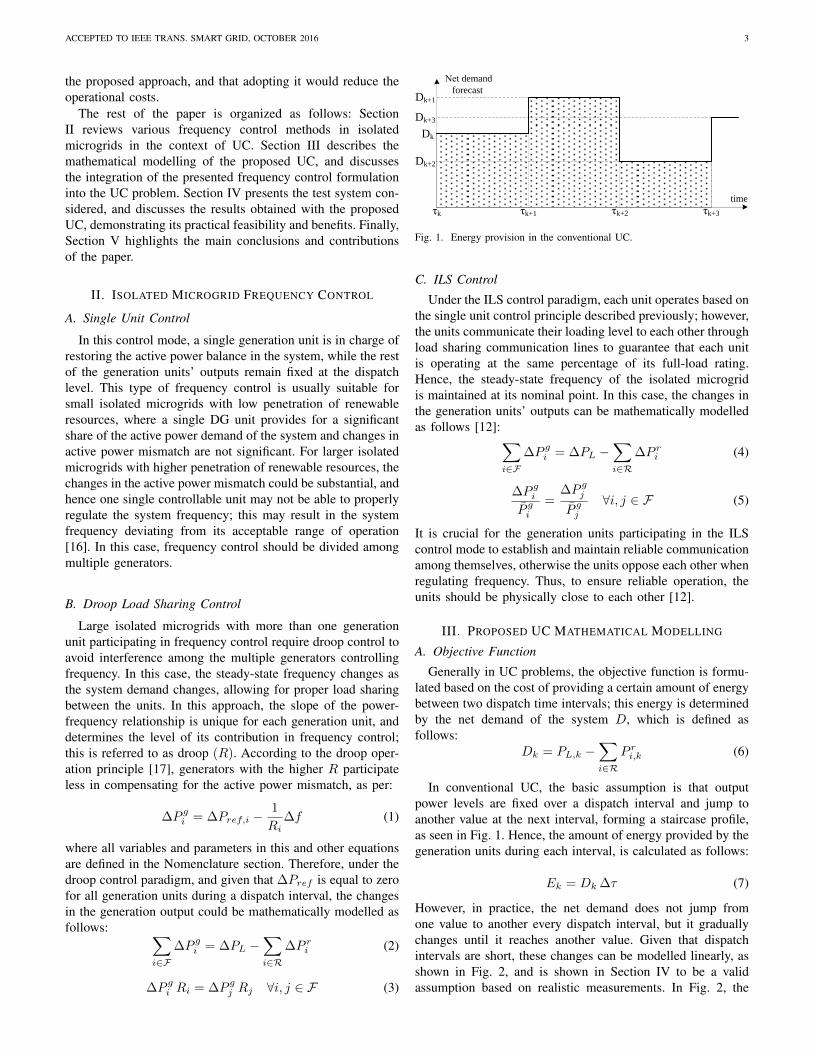
Fig. 1. Energy provision in the conventional UC.

C. ILS Control

Under the ILS control paradigm, each unit operates based onthe single unit control principle described previously; however,the units communicate their loading level to each other throughload sharing communication lines to guarantee that each unitis operating at the same percentage of its full-load rating.Hence, the steady-state frequency of the isolated microgridis maintained at its nominal point. In this case, the changes inthe generation units’ outputs can be mathematically modelledas follows [12]:∑

i∈F∆P gi = ∆PL −

∑i∈R

∆P ri (4)

∆P giP gi

=∆P gjP gj

∀i, j ∈ F (5)

It is crucial for the generation units participating in the ILScontrol mode to establish and maintain reliable communicationamong themselves, otherwise the units oppose each other whenregulating frequency. Thus, to ensure reliable operation, theunits should be physically close to each other [12].

III. PROPOSED UC MATHEMATICAL MODELLING

A. Objective Function

Generally in UC problems, the objective function is formu-lated based on the cost of providing a certain amount of energybetween two dispatch time intervals; this energy is determinedby the net demand of the system D, which is defined asfollows:

Dk = PL,k −∑i∈R

P ri,k (6)

In conventional UC, the basic assumption is that outputpower levels are fixed over a dispatch interval and jump toanother value at the next interval, forming a staircase profile,as seen in Fig. 1. Hence, the amount of energy provided by thegeneration units during each interval, is calculated as follows:

Ek = Dk ∆τ (7)

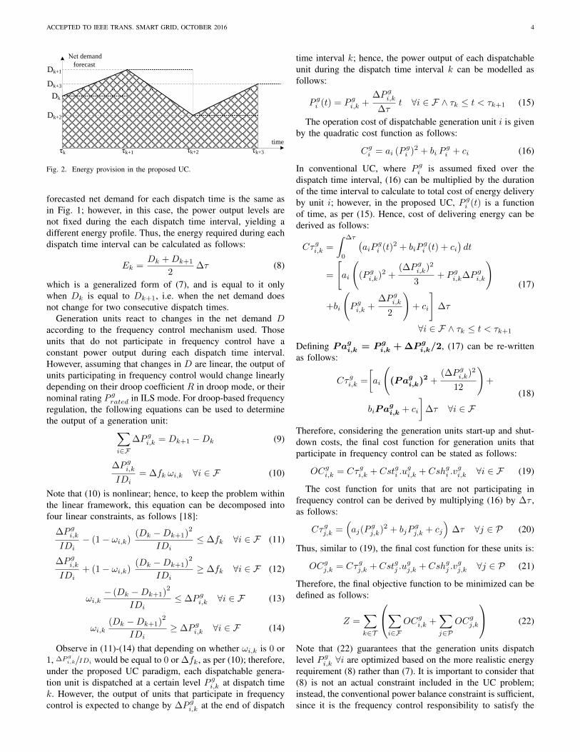
However, in practice, the net demand does not jump fromone value to another every dispatch interval, but it graduallychanges until it reaches another value. Given that dispatchintervals are short, these changes can be modelled linearly, asshown in Fig. 2, and is shown in Section IV to be a validassumption based on realistic measurements. In Fig. 2, the


time

Net demand forecast

τk+1τk τk+2 τk+3

Dk+1

Dk

Dk+3

Dk+2

Fig. 2. Energy provision in the proposed UC.

forecasted net demand for each dispatch time is the same asin Fig. 1; however, in this case, the power output levels arenot fixed during the each dispatch time interval, yielding adifferent energy profile. Thus, the energy required during eachdispatch time interval can be calculated as follows:

Ek =Dk +Dk+1

2∆τ (8)

which is a generalized form of (7), and is equal to it onlywhen Dk is equal to Dk+1, i.e. when the net demand doesnot change for two consecutive dispatch times.

Generation units react to changes in the net demand Daccording to the frequency control mechanism used. Thoseunits that do not participate in frequency control have aconstant power output during each dispatch time interval.However, assuming that changes in D are linear, the output ofunits participating in frequency control would change linearlydepending on their droop coefficient R in droop mode, or theirnominal rating P grated in ILS mode. For droop-based frequencyregulation, the following equations can be used to determinethe output of a generation unit:∑

i∈F∆P gi,k = Dk+1 −Dk (9)

∆P gi,kIDi

= ∆fk ωi,k ∀i ∈ F (10)

Note that (10) is nonlinear; hence, to keep the problem withinthe linear framework, this equation can be decomposed intofour linear constraints, as follows [18]:

∆P gi,kIDi

− (1− ωi,k)(Dk −Dk+1)

2

IDi≤ ∆fk ∀i ∈ F (11)

∆P gi,kIDi

+ (1− ωi,k)(Dk −Dk+1)

2

IDi≥ ∆fk ∀i ∈ F (12)

ωi,k− (Dk −Dk+1)

2

IDi≤ ∆P gi,k ∀i ∈ F (13)

ωi,k(Dk −Dk+1)

2

IDi≥ ∆P gi,k ∀i ∈ F (14)

Observe in (11)-(14) that depending on whether ωi,k is 0 or1, ∆P g

i,k/IDi would be equal to 0 or ∆fk, as per (10); therefore,under the proposed UC paradigm, each dispatchable genera-tion unit is dispatched at a certain level P gi,k at dispatch timek. However, the output of units that participate in frequencycontrol is expected to change by ∆P gi,k at the end of dispatch

time interval k; hence, the power output of each dispatchableunit during the dispatch time interval k can be modelled asfollows:

P gi (t) = P gi,k +∆P gi,k∆τ

t ∀i ∈ F ∧ τk ≤ t < τk+1 (15)

The operation cost of dispatchable generation unit i is givenby the quadratic cost function as follows:

Cgi = ai (P gi )2 + bi Pgi + ci (16)

In conventional UC, where P gi is assumed fixed over thedispatch time interval, (16) can be multiplied by the durationof the time interval to calculate to total cost of energy deliveryby unit i; however, in the proposed UC, P gi (t) is a functionof time, as per (15). Hence, cost of delivering energy can bederived as follows:

Cτgi,k =

∫ ∆τ

0

(aiP

gi (t)2 + biP

gi (t) + ci

)dt

=

[ai

((P gi,k)2 +

(∆P gi,k)2

3+ P gi,k∆P gi,k

)

+bi

(P gi,k +

∆P gi,k2

)+ ci

]∆τ

∀i ∈ F ∧ τk ≤ t < τk+1

(17)

Defining Pagi,k = P g

i,k + ∆P gi,k/2, (17) can be re-written

as follows:

Cτgi,k =

[ai

((Pag

i,k)2 +(∆P gi,k)2

12

)+

biPagi,k + ci

]∆τ ∀i ∈ F

(18)

Therefore, considering the generation units start-up and shut-down costs, the final cost function for generation units thatparticipate in frequency control can be stated as follows:

OCgi,k = Cτgi,k + Cstgi .ugi,k + Cshgi .v

gi,k ∀i ∈ F (19)

The cost function for units that are not participating infrequency control can be derived by multiplying (16) by ∆τ ,as follows:

Cτgj,k =(aj(P

gj,k)2 + bjP

gj,k + cj

)∆τ ∀j ∈ P (20)

Thus, similar to (19), the final cost function for these units is:

OCgj,k = Cτgj,k + Cstgj .ugj,k + Cshgj .v

gj,k ∀j ∈ P (21)

Therefore, the final objective function to be minimized can bedefined as follows:

Z =∑k∈T

∑i∈F

OCgi,k +∑j∈P

OCgj,k

(22)

Note that (22) guarantees that the generation units dispatchlevel P gi,k ∀i are optimized based on the more realistic energyrequirement (8) rather than (7). It is important to consider that(8) is not an actual constraint included in the UC problem;instead, the conventional power balance constraint is sufficient,since it is the frequency control responsibility to satisfy the


power balance during the rest of the time interval, thusensuring that the energy required is supplied by the generationunits. Since the changes in the generation unit output due tofrequency control is properly modelled in (22), the overall UCis guaranteed to consider and optimize for these changes.

Observe that the procedure used here to obtain the finalobjective function can be applied to any other linear ornonlinear heat-rate function. Furthermore, even though (11) isdeveloped based on droop-based control, it can be modified toaccount for either single-unit or ILS control. For the former,the set F only contains a single generation unit index, andthere is no need for (10)-(14); for the latter, To model the ILScontrol mode, IDi should be replaced by P grated,i in (10)-(14).

B. Operating Constraints

1) Power Balance: Similar to conventional UC, the pro-posed UC requires that the generated power and demand beequal at each dispatch time, yielding the following constraints:∑i∈G

P gi,k +∑i∈R

P ri,k +∑i∈S

(P s,dchi,k − P s,chgi,k

)− PL,k = 0

∀k ∈ T(23)

2) Dispatchable Units: There are certain constraints as-sociated with dispatchable generation units such as accept-able power generation range, ramp-up and ramp-down limits,minimum-up and minimum-down time limits, and coordina-tion constraints,, which are modelled as follows [19]:

¯P gi ωi,k ≤ P

gi,k ≤ P

gi ωi,k ∀i ∈ G ∧ k ∈ T (24)

P gi,k+1 − Pgi,k ≤ R

gi∆τ + ugi,k¯

P gi ∀i ∈ P ∧ k ∈ T (25)

P gi,k − Pgi,k+1 ≤ ¯

Rgi∆τ + vgi,k¯P gi ∀i ∈ P ∧ k ∈ T (26)

ugi,k − ugi,k−1 − u

gi,t ≤ 0 ∀i ∈ G ∧ k ∈ T ∗ ∧ t ∈ T1 (27)

ugi,k−1 − ugi,k + ugi,t ≤ 1 ∀i ∈ G ∧ k ∈ T ∗ ∧ t ∈ T2 (28)

ugi,k − vgi,k = ωgi,k − ω

gi,k−1 ∀i ∈ G ∧ k ∈ T (29)

ugi,k + vgi,k ≤ 1 ∀i ∈ G ∧ k ∈ T (30)

where,

T1 = {t+ 1, . . . ,min{t+MUgi − 1, lenght(τ)}}T2 = {t+ 1, . . . ,min{t+MDg

i − 1, lenght(τ)}}(31)

Equation (24) ensures that the output power of dispatchableunits remains within the acceptable operation limit. Equations(25) and (26) guarantee that the dispatchable units do noexceed their ramp-up and ramp-down limits. Please note thatthese ramping constraints are relaxed for units that participatein frequency control, since these units have a much fasterresponse aligned with the frequency control requirements [12].Minimum-up and minimum-down time limits are modelled in(27) and (28). Finally, coordination constraints are modelledin (29) and (30).

Furthermore, for ILS control, another constraint is includedto ensure that each unit is operating at the same percentage ofits full-load rating, as follows [12]:

P gj,k

∑i∈F

ωgi,kPgi − P

gj ω

gj,k

∑i∈F

P gi,k = 0 ∀j ∈ F (32)

Since this constraint is nonlinear, it should be decomposedin its linear equivalent constraints; hence, a new auxiliaryvariable αgi,j,k = ωgi,kP

gj,k is defined, resulting in the following

set of constraints:∑i∈F

αgi,j,kPgi − P

gj

∑i∈F

αgj,i,k = 0 ∀j ∈ F (33)

0 ≤ αgi,j,k ≤ ωgi,kP

gj,k ∀i, j ∈ F (34)

P gj,k −(

1− ωgi,k)P gj ≤ α

gi,j,k ≤ P

gj,k +

(1− ωgi,k

)P gj

∀i, j ∈ F (35)

3) ESS: The following set of constraints are included toproperly model the ESS behaviour:

SOC i ≤ SOCi,k ≤ SOCi ∀i ∈ S ∧ k ∈ T (36)

SOCi,k+1 − SOCi,k =

(P s,chgi,k ηi −

P s,dchi,k

ηi

)∆τ

∀i ∈ S ∧ k ∈ T(37)

0 ≤ P s,chgi,k ≤ P si(1− dsi,k

)∀i ∈ P ∧ k ∈ T (38)

0 ≤ P s,dchi,k ≤ P si dsi,k ∀i ∈ P ∧ k ∈ T (39)

The SOC maximum and minimum limit constraints and theSOC evolution model over time are modelled in (36) and(37). Also, (38) and (39) make sure that the ESS charge anddischarge powers are within a certain range and would nottake place simultaneously.

C. Reserve Constraints

Adequate reserves play a key role in proper frequencycontrol, and hence it should be carefully modelled in the UCproblem; however, most of the previous works that propose alinear UC either neglect reserve constraints or apply it only tothe largest generator in the system. This approach is not ade-quate for either droop control or ILS control, because multiplegenerators participate in regulating the system frequency andthe reserve constraint should be applied to all participants asan aggregate. Therefore, the reserve constraint is representedhere as follows:∑

i∈F

(ωgi,kP

gi − P

gi,k

)≥ RESk ∀k ∈ T (40)

In this paper, RESk is considered to be 10% of PL,k. Fur-thermore, at least one of the units that participate in frequencycontrol should be committed at every dispatch time step, whichcan be enforced as follows:∑

i∈Fωgi,k ≥ 1 ∀k ∈ τ (41)


D2

1

2

3

4

5

11

10

9

8

7

6

12

13

4.4 km

0.6 km

4.9 km

2.0 km

3.0 km

1.7 km

0.2 km

0.5 km0.6 km

D3 D4D1

D5

120 kW

80 kW

120 kW 200 kW

160 kW 120 kW

120 kW

80 kW

1500

kW

3000

kW

2000

kW

500

kW3000

kW

1.7 km

0.3 km

1.3 km

2.8 km

1.5 km

600 kW

2250 kW

1500 kW

1200 kW

1500 kW

600 kW

1800 kW

1800 kW

1000 kW

1000 kW 1000 kW

750 KW

BusLoad

PV WindESS

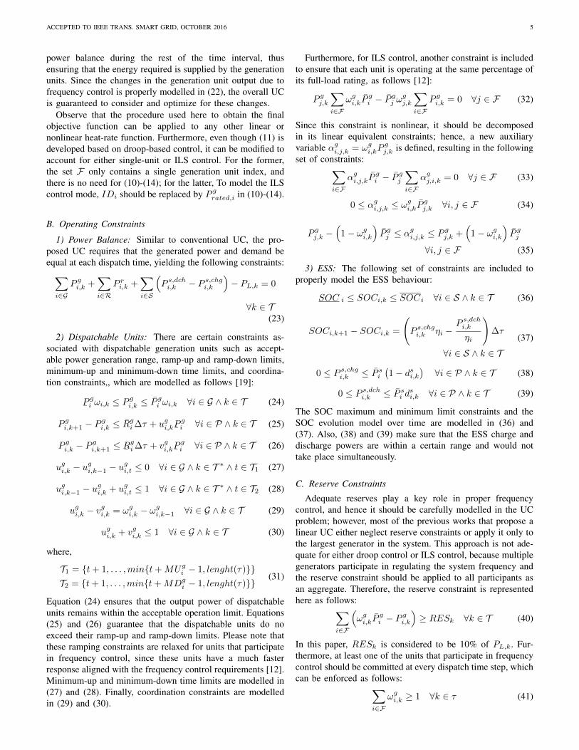
Fig. 3. Cigre benchmark system for medium voltage netwrok.

Finally, it should be ensured that the output of dispatchableunits that participate in frequency control will remain withinacceptable generation limits during the dispatch time interval;this can be enforced as follows:

¯P gi ≤ PE

gi,k ≤ P

gi ∀i ∈ F ∧ k ∈ T (42)

where PEgi,k is given from (15) as: PEg

i,k = P gi (τk+1).

Note that (42) is different from the conventional UC constraintthat requires the dispatch values to be within an acceptablerange, only at the beginning of the dispatch interval.

IV. RESULTS AND DISCUSSIONS

To test and validate the efficiency of the proposed UCfor isolated microgrids, a modified version of the CIGREbenchmark system for medium voltage networks is used [20],as shown in Fig. 3. The test system has a total installedcapacity of 27 MW, with 5 diesel engines, ESS, and windand PV based renewable energy resources. The peak load inthe system is around 15 MW. Nominal ratings of the dieselengines are given in Table I; the nominal rating of the windturbine is 8000 kW and of the PV unit is 1000 kW. Units D1,D3, and D4 participate in frequency control. Typical valuesare assumed for parameters and heat-rates corresponding tothe diesel engines [19]. For the ESS, ESS1 has a maximumpower rating of 1500 kW, a maximum energy rating of 5000kWh, and a minimum allowable SOC of 300 kWh; and ESS2has a maximum power rating of 500 kW, a maximum energyrating of 1000 kWh, and a minimum allowable SOC of 150kWh. In all test cases, the wind, PV, and load profiles arebased on high resolution (1 s) realistic measurements from anactual isolated/remote microgrid.

The performance of the proposed UC is tested over 24 h ofoperation, and a dispatch time interval of 5 min. The MIQPmodel is coded in GAMS [21], and is solved using the CPLEX

TABLE IDIESEL GENERATORS PARAMETERS

D1 D2 D3 D4 D5

ai ($/kWh2) 0.00015 0.00025 0.00015 0.00010 0.0005

bi ($/kWh) 0.2881 0.2876 0.2571 0.224 0.3476

ci ($/h) 7.5 0 25.5 45.5 0

Cstgi ($) 15 7.35 45 95 10

Cshgi ($) 5.3 1.44 8.3 15.3 0

IDi (kW/Hz) 4000 - 2000 5000 -

P gi (kW) 5000 1500 4000 6000 1000

¯P gi (kW) 180 100 150 200 100

0

2000

4000

6000

8000

0 50 100 150 200 250 300N

et d

eman

d (

kW

)t (s)

Proposed UC

Actual Measurement

Fig. 4. Case A actual used measurements of and assumed net demand.

TABLE IICASE A PROPOSED UC VS. CONVENTIONAL UC

UC P g1 P g

3 P g4 Objective Actual CPU

(kW) (kW) (kW) Function ($) Cost ($) Time (s)

Conv. 2777 1857 4231 471 299 1.45

Prop. 2591 2276 3998 303 296 1.45

solver [22]. The benefits of the proposed UC are demonstratedthrough several test case studies described next.

A. Case A: Proof of Concept

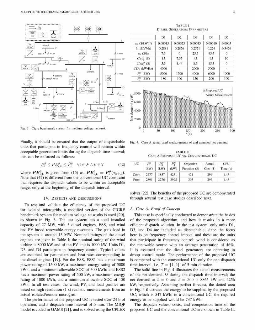
This case is specifically conducted to demonstrate the basicsof the proposed algorithm, and how it results in a moreefficient dispatch solution. In the test system, only units D1,D3, and D4 are included as dispatchable, since the focushere is on frequency control impact, and these are the unitsthat participate in frequency control; wind is considered asthe renewable source with an average penetration of 46%.It is assumed that the diesel generators are operating indroop control mode. The performance of the proposed UCis compared with the conventional UC only for one dispatchtime interval, i.e. T = {1, 2}, of 5 min duration.

The solid line in Fig. 4 illustrates the actual measurementsof the net demand D during the dispatch time interval; thenet demand at t = 0 and t = 300 is 8865 kW and 4256kW, respectively. Assuming perfect forecast, the dotted areain Fig. 4 illustrates the energy to be supplied by the proposedUC, which is 547 kWh; in a conventional UC, the requiredenergy to be supplied would be 737 kWh.

The dispatch values, costs, and computation time of theproposed UC and the conventional UC are shown in Table II.


0

4000

8000

12000

16000

0 250 500 750 1000 1250

Po

wer

(k

W)

t (min)

Wind PV Load

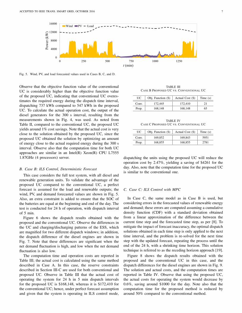
Fig. 5. Wind, PV, and load forecasted values used in Cases B, C, and D.

Observe that the objective function value of the conventionalUC is considerably higher than the objective function valueof the proposed UC, indicating that conventional UC overes-timates the required energy during the dispatch time interval,dispatching 737 kWh compared to 547 kWh in the proposedUC. To calculate the actual operation cost, the output of thediesel generators for the 300 s interval, resulting from themeasurements shown in Fig. 4, was used. As noted fromTable II, compared to the conventional UC, the proposed UCyields around 1% cost savings. Note that the actual cost is veryclose to the solution obtained by the proposed UC, since theproposed UC obtained the solution by optimizing an amountof energy close to the actual required energy during the 300 sinterval. Observe also that the computation time for both UCapproaches are similar in an Intel(R) Xeon(R) CPU L75551.87GHz (4 processors) server.

B. Case B: ILS Control, Deterministic Forecast

This case considers the full test system, with all diesel andrenewable generation units. To validate the advantage of theproposed UC compared to the conventional UC, a perfectforecast is assumed for the load and renewable outputs; thewind, PV, and demand forecasted values are shown in Fig. 5.Also, an extra constraint is added to ensure that the SOC ofthe batteries are equal at the beginning and end of the day. Thetest is conducted for 24 h of operation, with dispatch intervalof 5 min.

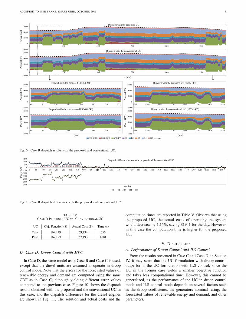
Figure 6 shows the dispatch results obtained with theproposed and the conventional UC. Observe the differences inthe UC and charging/discharging patterns of the ESS, whichare magnified for two different dispatch windows; in addition,the dispatch difference of the diesel engines are shown inFig. 7. Note that these differences are significant when thenet demand fluctuation is high, and low when the net demandfluctuation is also low.

The computation time and operation costs are reported inTable III; the actual cost is calculated using the same methoddescribed in Case A. In this case, the reserve constraintsdescribed in Section III-C are used for both conventional andproposed UC. Observe in Table III that the actual cost ofoperating the system for 24 h in 5 min dispatch intervalsfor the proposed UC is $168,148, whereas it is $172,410 forthe conventional UC; hence, under perfect forecast assumptionand given that the system is operating in ILS control mode,

TABLE IIICASE B PROPOSED UC VS. CONVENTIONAL UC

UC Obj. Function ($) Actual Cost ($) Time (s)

Conv. 172,445 172,410 21

Prop. 168,148 168,148 65

TABLE IVCASE C PROPOSED UC VS. CONVENTIONAL UC


Conv. 169,852 169,843 5951

Prop. 168,855 168,855 2781

dispatching the units using the proposed UC will reduce theoperation cost by 2.47%, yielding a saving of $4261 for theday. Also, note that the computation time for the proposed UCis similar to the conventional one.

C. Case C: ILS Control with MPC

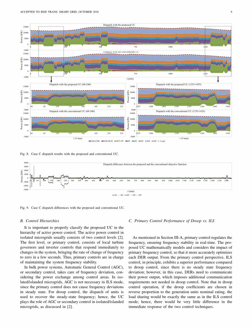
In Case C, the same model as in Case B is used, butconsidering errors in the forecasted values of renewable energyand demand; these errors are computed assuming a cumulativedensity function (CDF) with a standard deviation obtainedfrom a linear approximation of the difference between thecurrent time step and the forecasted time step, as per [8]. Tomitigate the impact of forecast inaccuracy, the optimal dispatchsolutions obtained in each time step is only applied to the nexttime interval, and the problem is re-solved for the next timestep with the updated forecast, repeating the process until theend of the 24 h, with a shrinking time horizon. This solutiontechnique is referred to as the receding horizon approach [19].

Figure 8 shows the dispatch results obtained with theproposed and the conventional UC in this case, and thedispatch differences for the diesel engines are shown in Fig. 9.The solution and actual costs, and the computation times arereported in Table IV. Observe that using the proposed UC,the actual costs for operating the system would decrease by0.6%, saving around $1000 for the day. Note also that thecomputation time for the proposed method is reduced byaround 50% compared to the conventional method.


-5000

0

5000

10000

15000

0 250 500 750 1000 1250

Po

wer

(k

W)

t (min)

Dispatch with the proposed objective function

ESS-CHG ESS-DCH WT+PV D1 D2 D3 D4 D5 Load

-5000

0

5000

10000

15000

0 250 500 750 1000 1250

Po

wer

(k

W)

t (min)



-5000

0

5000

10000

15000

0 250 500 750 1000 1250

Po

wer

(k

W)

t (min)

Dispatch with the conventional objective function


-5000

0

5000

10000

15000

1255 1280 1305 1330 1355 1380 1405 1430

Po

wer

(k

W)

t (5-min)

Dispatch with the proposed objective function (1255-1435)

Series1 Series2 Series3 Series4 Series5 Series6 Series7 Series8 Series9

-5000

0

5000

10000

15000

1255 1280 1305 1330 1355 1380 1405 1430

Po

wer

(k

W)

t (min)

Dispatch with the conventional objective function (1255-1435)


-5000

-5000 -5000-5000

0

5000

10000

15000

60 85 110 135 160 185 210 235

Po

wer

(k

W)

t (5-min)

Dispatch with the proposed objective function (60-240)


-5000

0

5000

10000

15000

60 85 110 135 160 185 210 235

Po

wer

(k

W)

t (min)

Dispatch with the conventional objective function (60-240)


-5000

0

5000

10000

15000

0 250 500 750 1000 1250

Po

wer

(k

W)

t (min)



Dispatch with the conventional UC

Dispatch with the proposed UC

Dispatch with the proposed UC (60-240)

Dispatch with the conventional UC (60-240)



Fig. 6. Case B dispatch results with the proposed and conventional UC.

-3000

-2500

-2000

-1500

-1000

-500

0

500

1000

1500

0 50 100 150 200 250 300 350 400 450 500 550 600 650 700 750 800 850 900 950 1000 1050 1100 1150 1200 1250 1300 1350 1400

Pow

er (

kW

)

t (min)

Dispatch difference between the proposed and the conventional UC

D1 D2 D3 D4 D5

Fig. 7. Case B dispatch differences with the proposed and conventional UC.

TABLE VCASE D PROPOSED UC VS. CONVENTIONAL UC


Conv. 169,149 169,134 656

Prop. 167,193 167,193 1001

D. Case D: Droop Control with MPC

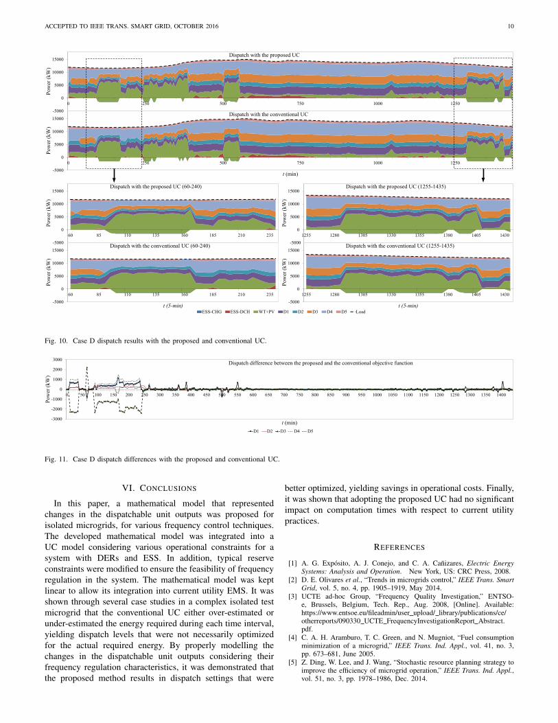
In Case D, the same model as in Case B and Case C is used,except that the diesel units are assumed to operate in droopcontrol mode. Note that the errors for the forecasted values ofrenewable energy and demand are computed using the sameCDF as in Case C, although yielding different error valuescompared to the previous case. Figure 10 shows the dispatchresults obtained with the proposed and the conventional UC inthis case, and the dispatch differences for the diesel enginesare shown in Fig. 11. The solution and actual costs and the

computation times are reported in Table V. Observe that usingthe proposed UC, the actual costs of operating the systemwould decrease by 1.15%, saving $1941 for the day. However,in this case the computation time is higher for the proposedUC.

V. DISCUSSIONS

A. Performance of Droop Control and ILS Control

From the results presented in Case C and Case D, in SectionIV, it may seem that the UC formulation with droop controloutperforms the UC formulation with ILS control, since theUC in the former case yields a smaller objective functionand takes less computational time. However, this cannot begeneralized, as the performance of the UC in droop controlmode and ILS control mode depends on several factors suchas the droop coefficients, the generators nominal rating, theforecasted values of renewable energy and demand, and otherparameters.


-5000

0

5000

10000

15000

0 250 500 750 1000 1250

Po

wer

(k

W)

t (min)



-5000

0

5000

10000

15000

1255 1280 1305 1330 1355 1380 1405 1430

Pow

er (

kW

)

t (5-min)



-5000

0

5000

10000

15000

1255 1280 1305 1330 1355 1380 1405 1430

Pow

er (

kW

)

t (5-min)



-5000

0

5000

10000

15000

0 250 500 750 1000 1250

Pow

er (

kW

)

t (min)



-5000

0

5000

10000

15000

0 250 500 750 1000 1250

Po

wer

(k

W)

t (min)



-5000

0

5000

10000

15000

60 85 110 135 160 185 210 235

Pow

er (

kW

)

t (5-min)



-5000

0

5000

10000

15000

60 85 110 135 160 185 210 235

Pow

er (

kW

)

t (5-min)



-5000

-5000

-5000

0

5000

10000

15000

0 250 500 750 1000 1250

Pow

er (

kW

)

t (min)



-5000

Fig. 8. Case C dispatch results with the proposed and conventional UC.

-3000

-2000

-1000

0

1000

2000

3000

4000

0 50 100 150 200 250 300 350 400 450 500 550 600 650 700 750 800 850 900 950 1000 1050 1100 1150 1200 1250 1300 1350 1400Po

wer

(k

W)

t (min)

Dispatch difference between the proposed and the conventional objective function

D1 D2 D3 D4 D5

Fig. 9. Case C dispatch differences with the proposed and conventional UC.

B. Control Hierarchies

It is important to properly classify the proposed UC in thehierarchy of active power control. The active power control inisolated microgrids usually consists of two control levels [2].The first level, or primary control, consists of local turbinegovernors and inverter controls that respond immediately tochanges in the system, bringing the rate of change of frequencyto zero in a few seconds. Thus, primary controls are in chargeof maintaining the system frequency stability.

In bulk power systems, Automatic General Control (AGC),or secondary control, takes care of frequency deviation, con-sidering the power exchange among control areas. In iso-lated/islanded microgrids, AGC is not necessary in ILS mode,since the primary control does not cause frequency deviationsin steady state. For droop control, the dispatch of units isused to recover the steady-state frequency; hence, the UCplays the role of AGC or secondary control in isolated/islandedmicrogrids, as discussed in [2].

C. Primary Control Performance of Droop vs. ILS

As mentioned in Section III-A, primary control regulates thefrequency, ensuring frequency stability in real-time. The pro-posed UC mathematically models and considers the impact ofprimary frequency control, so that it more accurately optimizeseach DER output. From the primary control perspective, ILScontrol, in principle, exhibits a superior performance comparedto droop control, since there is no steady state frequencydeviation; however, in this case, DERs need to communicatetheir power output, which imposes additional communicationrequirements not needed in droop control. Note that in droopcontrol operation, if the droop coefficients are chosen inreverse proportion to the generation units nominal rating, theload sharing would be exactly the same as in the ILS controlmode; hence, there would be very little difference in theimmediate response of the two control techniques.


-5000

0

5000

10000

15000

0 250 500 750 1000 1250

Po

wer

(k

W)

t (min)



-5000

0

5000

10000

15000

0 250 500 750 1000 1250

Po

wer

(k

W)

t (min)



-5000

0

5000

10000

15000

0 250 500 750 1000 1250

Po

wer

(k

W)

t (min)



-5000

-5000

0

5000

10000

15000

1255 1280 1305 1330 1355 1380 1405 1430

Po

wer

(k

W)

t (5-min)



-5000

0

5000

10000

15000

60 85 110 135 160 185 210 235

Po

wer

(k

W)

t (5-min)



-5000

0

5000

10000

15000

60 85 110 135 160 185 210 235

Po

wer

(k

W)

t (5-min)



-5000

-5000

0

5000

10000

15000

1255 1280 1305 1330 1355 1380 1405 1430

Po

wer

(k

W)

t (5-min)



-5000

-5000

0

5000

10000

15000

0 250 500 750 1000 1250

Po

wer

(k

W)

t (min)



Fig. 10. Case D dispatch results with the proposed and conventional UC.

-3000

-2000

-1000

0

1000

2000

3000

0 50 100 150 200 250 300 350 400 450 500 550 600 650 700 750 800 850 900 950 1000 1050 1100 1150 1200 1250 1300 1350 1400

Pow

er (

kW

)

t (min)

Dispatch difference between the proposed and the conventional objective function

D1 D2 D3 D4 D5

Fig. 11. Case D dispatch differences with the proposed and conventional UC.

VI. CONCLUSIONS

In this paper, a mathematical model that representedchanges in the dispatchable unit outputs was proposed forisolated microgrids, for various frequency control techniques.The developed mathematical model was integrated into aUC model considering various operational constraints for asystem with DERs and ESS. In addition, typical reserveconstraints were modified to ensure the feasibility of frequencyregulation in the system. The mathematical model was keptlinear to allow its integration into current utility EMS. It wasshown through several case studies in a complex isolated testmicrogrid that the conventional UC either over-estimated orunder-estimated the energy required during each time interval,yielding dispatch levels that were not necessarily optimizedfor the actual required energy. By properly modelling thechanges in the dispatchable unit outputs considering theirfrequency regulation characteristics, it was demonstrated thatthe proposed method results in dispatch settings that were

better optimized, yielding savings in operational costs. Finally,it was shown that adopting the proposed UC had no significantimpact on computation times with respect to current utilitypractices.

REFERENCES

[1] A. G. Exposito, A. J. Conejo, and C. A. Canizares, Electric EnergySystems: Analysis and Operation. New York, US: CRC Press, 2008.

[2] D. E. Olivares et al., “Trends in microgrids control,” IEEE Trans. SmartGrid, vol. 5, no. 4, pp. 1905–1919, May 2014.

[3] UCTE ad-hoc Group, “Frequency Quality Investigation,” ENTSO-e, Brussels, Belgium, Tech. Rep., Aug. 2008, [Online]. Available:https://www.entsoe.eu/fileadmin/user upload/ library/publications/ce/otherreports/090330 UCTE FrequencyInvestigationReport Abstract.pdf.

[4] C. A. H. Aramburo, T. C. Green, and N. Mugniot, “Fuel consumptionminimization of a microgrid,” IEEE Trans. Ind. Appl., vol. 41, no. 3,pp. 673–681, June 2005.

[5] Z. Ding, W. Lee, and J. Wang, “Stochastic resource planning strategy toimprove the efficiency of microgrid operation,” IEEE Trans. Ind. Appl.,vol. 51, no. 3, pp. 1978–1986, Dec. 2014.


[6] H. Kanchev, F. Colas, V. Lazarov, and B. Francois, “Emission reductionand economical optimization of an urban microgrid operation includingdispatched pv-based active generators,” IEEE Trans. Sustain. Energy,vol. 5, no. 4, pp. 1397–1405, July 2014.

[7] R. Palma-Behnke, C. Benavides, F. Lanas, B. Severino, L. Reyes,J. Llanos, and D. Saez, “A microgrid energy management system basedon the rolling horizon strategy,” IEEE Trans. Smart Grid, vol. 4, no. 2,pp. 994–1006, Jan. 2013.

[8] B. V. Solanki, A. Raghurajan, K. Bhattacharya, and C. A. Canizares,“Including smart loads for optimal demand response in integrated energymanagement systems for isolated microgrids,” IEEE Trans. Smart Grid,in print.

[9] Y. C. Wu, M. J. Chen, J. Y. Lin, W. S. Chen, and W. L. Huang,“Corrective economic dispatch in a microgrid,” Int. J. Numer. Model.Electron. Netw. Devices Fields, vol. 26, no. 2, pp. 140–150, June 2012.

[10] J. W. O’Sullivan and M. J. O’Malley, “A new methodology for theprovision of reserve in an isolated power system,” IEEE Trans. PowerSyst., vol. 14, no. 2, pp. 519–524, May 1999.

[11] G. W. Chang, C. Ching-Sheng, L. Tai-Ken, and W. Ching-Chung,“Frequency-regulating reserve constrained unit commitment for an iso-lated power system,” IEEE Trans. Power Syst., vol. 28, no. 2, pp. 578–586, Aug. 2012.

[12] A. H. Hajimiragha, M. R. D. Zadeh, and S. Moazeni, “Microgridsfrequency control considerations within the framework of the optimalgeneration scheduling problem,” IEEE Trans. Smart Grid, vol. 6, no. 2,pp. 534–547, March 2013.

[13] G. X. Guan, F. Gao, and A. J. Svoboda, “Energy delivery capacity andgeneration scheduling in the deregulated electric power market,” IEEETrans. Power Syst., vol. 15, no. 4, pp. 1275–1280, Nov. 2000.

[14] Y. Yang, J. Wang, X. Guan, and Q. Zhai, “Subhourly unit commitmentwith feasible energy delivery constraints,” Appl. Energy, vol. 96, pp.245–252, Aug. 2012.

[15] G. Morales-Espana, A. Ramos, and J. Garcia-Gonzalez, “An MIPformulation for joint market-clearing of energy and reserves based onramp scheduling,” IEEE Trans. Power Syst., vol. 29, no. 1, pp. 476–488,May 2013.

[16] C. Yuen, A. Oudalov, and A. Timbus, “The provision of frequencycontrol reserves from multiple microgrids,” IEEE Trans. Ind. Electron.,vol. 58, no. 1, pp. 173–183, Jan. 2011.

[17] P. Kundur, Power System Stability and Control. New York, US:McGraw-hill Professional, 1994.

[18] C. A. Floudas, Nonlinear and Mixed-Integer Optimization: Fundamen-tals and Applications. Oxford, UK: Oxford University Press, 1999.

[19] D. E. Olivares, C. A. Canizares, and M. Kazerani, “A centralized energymanagement system for isolated microgrids,” IEEE Trans. Smart Grid,vol. 5, no. 4, pp. 1864–1875, April 2014.

[20] K. Strunz, “Developing benchmark models for studying the integrationof distributed energy resources,” in Proc. IEEE Power Eng. Soc. Gen.Meeting, Montreal, QC, July 2006.

[21] R. E. Rosenthal, GAMS – A User’s Guide. Washington, DC, USA:GAMS Development Corporation, 2016.

[22] “IBM ILOG CPLEX V12.1 User’s Manual for CPLEX,” Inter-national Business Machines Corporation, Tech. Rep., 2009, [On-line]. Available: ftp://public.dhe.ibm.com/software/websphere/ilog/docs/optimization/cplex/ps usrmancplex.pdf.

Mostafa Farrokhabadi (S’12) received the B.Sc.degree in electrical engineering from Amirkabir Uni-versity of Technology, Tehran, Iran, in 2010, and theM.Sc. degree in Electric Power Engineering fromKTH Royal Institute of Technology, Stockholm,Sweden, in 2012. He is currently a Ph.D. candidatein the Electrical and Computer Engineering Depart-ment at the University of Waterloo, ON, Canada. Hisresearch interests includes modeling, control, andoptimization in microgrids.

Claudio A. Canizares (S’85, M’91, SM’00, F’07)received in April 1984 the Electrical EngineerDiploma from the Escuela Politecnica Nacional(EPN), Quito-Ecuador, where he held differentteaching and administrative positions from 1983 to1993. His MS (1988) and PhD (1991) degrees inElectrical Engineering are from the University ofWisconsin-Madison. He has held various academicand administrative positions at the E&CE Depart-ment of the University of Waterloo since 1993,where he is currently a full Professor and the Hydro

One Endowed Chair. His research activities concentrate on the study ofmodeling, simulation, control, stability, computational and dispatch issues insustainable power and energy systems in the context of competitive marketsand smart grids.

Kankar Bhattacharya Kankar Bhattacharya (M’95,SM’01) received the Ph.D. degree in Electrical Engi-neering from the Indian Institute of Technology, NewDelhi, India in 1993. He was in the faculty of IndiraGandhi Institute of Development Research, Mumbai,India, during 1993-1998, and then the Departmentof Electric Power Engineering, Chalmers Universityof Technology, Gothenburg, Sweden, during 1998-2002. He joined the E&CE Department of the Uni-versity of Waterloo, Canada, in 2003 where he iscurrently a full Professor. His research interests are

in power system economics and operational aspects.

Documents

ACCEPTED TO IEEE TRANS. SMART GRID, OCTOBER 2016 1 …ACCEPTED TO IEEE TRANS. SMART GRID, OCTOBER 2016 1 Unit Commitment for Isolated Microgrids Considering Frequency Control Mostafa