ACCEPTED MANUSCRIPT - Virginia Tech · · 2016-10-12ACCEPTED MANUSCRIPT Additive Gaussian Process for Computer Models With Qualitative and Quantitative Factors X. Deng†, C. Devon

ACCEPTED MANUSCRIPT

Additive Gaussian Process for Computer Models WithQualitative and Quantitative Factors

X. Deng†, C. Devon Lin‡1, K-W. Liu § andR.K. Rowe§§

†Department of Statistics, Virginia Tech

‡Department of Mathematics and Statistics, Queen’s University

§School of Civil Engineering, Southwest Jiaotong University

§§Department of Civil Engineering, Queen’s University

Abstract

Computer experiments with qualitative and quantitative factors occur frequently in various ap-

plications in science and engineering. Analysis of such experiments is not yet completely resolved.

In this work, we propose an additive Gaussian process model for computer experiments with quali-

tative and quantitative factors. The proposed method considers an additive correlation structure for

qualitative factors, and assumes that the correlation function for each qualitative factor and the cor-

relation function of quantitative factors are multiplicative. It inherits the flexibility of unrestrictive

correlation structure for qualitative factors by using the hypersphere decomposition, embracing

more flexibility in modeling the complex systems of computer experiments. The merits of the

proposed method are illustrated by several numerical examples and a real data application.

Keywords:Additive model; Computer experiment; Fractional factorial design; Hypersphere de-

composition; Kriging.

1Address for correspondence: C. Devon Lin, Associate Professor, Department of Mathematics and Statistics,Queen’s University, Kingston, ON Canada (E-mail: [email protected]).

1ACCEPTED MANUSCRIPT

ACCEPTED MANUSCRIPT

1 Introduction

Computer experiments that use complex computer models to study real systems have attracted wide

attentions in many science and engineering applications. Because computer models are typically

expensive in terms of computational time, an emulator (surrogate model) is often needed (Sacks et

al. 1989). An emulator can be used as a stand-in for a computer model and it is cornerstone for

further analysis such as optimization, sensitivity analysis and uncertainty quantification. The bulk

of the work on building emulators assume that the input factors in computer models are quantitative

(Santner et al. 2003) and those methods are not directly applicable to computer models that contain

both qualitative and quantitative factors.

Computer models with both qualitative and quantitative factors arise in various applications.

For example, this work is motivated by a real computer experiment of finite element modeling

of full-scale embankment over soft soils considering reinforcement stiffness and column length as

qualitative factors (Rowe and Liu 2015; Liu and Rowe 2015). Examples from the literature are: the

computational fluid-dynamics simulation for studying data center often contains qualitative factors

such as “hot air return vent location” and “power unit type” (Qian et al. 2008); the agent-based

network modeling in epidemiology study (Bhuiyan et al. 2014) often constructs the network with

shuffle type as a qualitative factor; for investigating wear mechanisms of total knee replacements

in bioengineering, Han et al. (2009) presents the knee models with qualitative factors such as

“prosthesis design” and “force pattern”.

Gaussian process modeling is a common technique for building emulators of computer models.

For computer models with both qualitative and quantitative factors, it is not trivial to build emula-

tors using Gaussian process modeling. This is because different level combinations of qualitative

factors may not have specific distance measurement. To accommodate both qualitative and quan-

titative factors into Gaussian process modeling, there are two key challenges: how to construct a

proper covariance structure for the qualitative factors, and how to specify the relationship between

the correlation function for qualitative factors and the correlation function for quantitative factors.

For constructing correlation function for qualitative factors, one approach is to consider a re-


ACCEPTED MANUSCRIPT

strictive correlation function (McMillian et al. 1999; Joseph and Delaney 2007). Such an approach

can simplify the computational complexity for the model estimation. However, restrictive cor-

relation functions lack flexibility to quantify general correlation structure of qualitative factors.

Another approach is to construct an unrestrictive correlation structure for qualitative factors. Qian

et al. (2008) developed a general framework of constructing an unrestrictive correlation structure

for qualitative factors in Gaussian process models. Their method adopts semi-definite optimiza-

tion in estimation to ensure the positive-definiteness of the correlation structure. To overcome the

complicated estimation procedure in Qian et al. (2008), Zhou et al. (2011) developed a hyper-

sphere parametrization (Pinheiro and Bates 1996; Rebonato and Jackel 1999) method to model

the unrestrictive correlation structure, which can automatically guarantee the positive-definiteness

of the correlation structure. Recently, Zhang and Notz (2015) considered an indicator function

approach to model the correlation function for the qualitative factors, which is in a similar spirit

as that in Zhou et al. (2011). The third direction is to adopt the hierarchical Bayesian Gaussian

process models (Swiler et al. 2014) to accommodate both qualitative and quantitative factors. For

constructing correlation functions with both qualitative and quantitative factors, the majority of ex-

isting work assumes the multiplication between the correlation function of qualitative factors and

the correlation function of quantitative factors. The potential drawback of using multiplication in

correlation function is that multiplication could improperly characterize the effect of the correla-

tion from qualitative factors. For example, when the correlation function of one qualitative factor

is small or close to zero, it would result in the overall correlation function to be very small.

In this work, we propose an additive Gaussian process model for computer experiments with

qualitative and quantitative factors. The key idea of the proposed method is to consider an additive

correlation structure for qualitative factors, and to assume that the correlation function for each

qualitative factor and the correlation function of quantitative factors are multiplicative. Such a for-

mulation also allows different covariance structures for quantitative factors with respect to different

qualitative factors. It inherits the flexibility of an unrestrictive correlation structure for qualitative

factors by using the hypersphere decomposition.

The remainder of this article is organized as follows. Section 2 provides notation and a gen-


ACCEPTED MANUSCRIPT

eral background. Section 3 details the proposed additive Gaussian process model, along with

the estimation, prediction and interpretation. Section 4 presents numerical examples to illustrate

the effectiveness of the proposed method. In Section 5, the proposed method is applied in a real

computer experiment of finite element modeling for full-scale embankment over soft soils. We

conclude this work with brief summary and discussion in Section 6.

2 Notation and Background

This section provides notation and background for later development. We review Gaussian pro-

cess models with only quantitative factors, and the hypersphere parameterization to construct the

correlation structure for qualitative factors in Zhou et al. (2011). Throughout, we consider com-

puter experiments withp quantitative factorsx = (x1, . . . , xp)T ∈ Rp and q qualitative factors

z = (z1, . . . , zq)T with the jth qualitative factor havingmj levels, j = 1, . . . , q, and the correspond-

ing output is denoted byY. Suppose that the data obtained from the computer experiment are

(yi ,wi), i = 1, . . . , n, wherewi = (xi , zi).

2.1 Gaussian Process Model with Quantitative Factors

With quantitative factors as inputs in the model, the key idea of Gaussian processes is to consider

the outputs from computer experiments as a realization of a Gaussian process. The correlation of

responses at two data points is determined by a correlation function of inputs, such as a Matern

correlation function (Matern 1986). To model the relationship between outputY and inputsx, one

stationary Gaussian process model, known as ordinary Kriging model, assumes,

Y(x) = μ + Z(x), (1)

whereμ is the constant mean,Z(x) is a Gaussian process with mean zero and the covariance func-

tionφ(∙) = σ2R(∙|θ). Hereσ2 is the variance andR(∙|θ) is referred to as the correlation function with

the correlation parameter vectorθ. A popular choice of the correlation function is the Gaussian


ACCEPTED MANUSCRIPT

correlation function

R(xi , x j |θ) = exp{−p∑

k=1

θk(xik − xjk)2}, (2)

for any two inputsxi = (xi1, . . . , xip)T and x j = (xj1, . . . , xjp)T, whereθ = (θ1, . . . , θp)T and

θk ≥ 0, k = 1, . . . , p. Consider the inputs of quantitative factorsx1, . . . , xn and the correspond-

ing responsesy1, . . . , yn. For the ordinary Kriging, the best linear predictor at an inputx is given

by

y(x) = μ + rT(x)R−1(y − μ1), (3)

wherey = (y1, . . . , yn)T, R is ann× n correlation matrix with the (i, j)th elementR(xi , x j), r (x) =

(R(x, x1), . . . ,R(x, xn))T, 1 is ann-dimensional column vector of all 1’s, and ˆμ = (1TR−11)−11TR−1y

is the estimate ofμ. Note that the predictor in (3) involves with unknown correlation parameters

in the correlation function. To estimate these parameters, a common approach is the maximum

likelihood estimation method (Santner et al. 2003; Fang et al. 2005).

2.2 Unrestrictive Correlation for Qualitative Factors

When computer experiments have qualitative factors as inputs, the usual correlation function in (2)

does not work properly because the Euclidian distance cannot be used for different level combi-

nations of qualitative factors. To address this issue, Zhou et al. (2011) introduced a hypersphere

parameterization to quantify the correlations of the qualitative factors. Recall that thejth qualita-

tive factorzj hasmj levels. Forj = 1, . . . , q, let T j = (τ( j)r,s) be anmj ×mj correlation matrix of the

mj levels of the qualitative factorzj. The key idea of Zhou et al. (2011) is to apply the hypersphere

decomposition to modelT j such thatT j is a positive-definite matrix with unit diagonal elements.

Their approach consists of two steps. Step 1 is to find a lower triangular matrix with strictly pos-

itive diagonal entriesL j = (l( j)r,s) through a Cholesky-type decomposition, that is,T j = L jLT

j for

j = 1, . . . , q. In Step 2, each row vector (l( j)r,1, . . . , l

( j)r,r ) in L j is specified in the following way: for


ACCEPTED MANUSCRIPT

r = 1, l j,1,1 = 1 and forr = 2, . . . ,mj,

l( j)r,1 = cos(ϕ j,r,1)

l( j)r,s = sin(ϕ j,r,1) ∙ ∙ ∙ sin(ϕ j,r,s−1)cos(ϕ j,r,s), for s= 2, . . . , r − 1

l( j)r,r = sin(ϕ j,r,1) ∙ ∙ ∙ sin(ϕ j,r,r−2)sin(ϕ j,r,r−1),

whereϕ j,r,s ∈ (0, π) andτ( j)r,r =

∑rs=1(l

( j)r,s)2 = 1 for r = 1, . . . ,mj.

For computer experiments with both quantitative factors and qualitative factors, Zhou et al. (2011)

combined the Gaussian correlation function for quantitative factors and hypersphere decomposi-

tion for qualitative factors. Specifically, for any two inputsw1 = (x1, z1) andw2 = (x2, z2), they

proposed the covariance betweenY(w1) andY(w2) to be

φ(Y(w1),Y(w2)) = σ2cor(Z(w1),Z(w2))

= σ2R(x1, x2|θ)q∏

j=1

τ( j)z1 j ,z2 j, (4)

whereR(x1, x2|θ) quantifies the correlation between inputsx1 and x2, andτ( j)z1 j ,z2 j represents the

correlation between levelz1 j and levelz2 j of the jth qualitative factor.

The correlation function in (4) considers the multiplicity of correlations between quantitative

factors and qualitative factors. Such a formulation may not be very flexible to accommodate the

complex effects of qualitative factors on the outputs of computer experiments. For example, a

zero value of anyτ( j)z1 j ,z2 j in (4) would result in the overall correlationφ(Y(w1),Y(w2)) being zero.

Therefore, it calls for novel, flexible correlation functions for modeling computer experiments with

both quantitative factors and qualitative factors.

3 Additive Gaussian Process Model

To enhance the flexibility in capturing the correlations between qualitative and quantitative factors

for accurate prediction, we propose a novel Gaussian process model to analyze data for com-

puter experiments with both qualitative and quantitative factors. For thep quantitative factors


ACCEPTED MANUSCRIPT

x = (x1, . . . , xp)T and theq qualitative factorsz = (z1, . . . , zq)T, we model the corresponding re-

sponseY as

Y(x, z1, . . . , zq) = μ + G1(z1, x) + ∙ ∙ ∙ + Gq(zq, x), (5)

whereμ is the overall mean,Gj ’s are independent Gaussian processes with mean zero and the

covariance functionφ j, for j = 1, . . . , q. Here we adopt the additive form to quantify the contri-

butions ofq qualitative input factors to the output. It is in a similar spirit to the additive model in

machine learning literature (Hastie and Tibshirani 1990). As the effects of qualitative factors on

responses are complicated, the motivation of the additive form is to emphasize the effect of each

qualitative factor coupled with quantitative factors. Moreover, the additive formulation enables us

to infer the significance of each individual qualitative factor in the model. The proposed model in

(5) incorporates interactions between qualitative factors and quantitative factors, and interactions

among quantitative factors. However, its current form does not take into account the interactions

among qualitative factors.

To construct the covariance functionφ j in each Gaussian processGj, we adopt the approach

in Zhou et al. (2011) for the qualitative factors. Recall that the correlation matrixT j = (τ( j)r,s) of

themj levels of the qualitative factorzj, j = 1, . . . , q. The covariance functionφ j for two inputs

w1 = (x1, z1) andw2 = (x2, z2) is given by

φ j(Gj(w1),Gj(w2)) = σ2j cor(Gj(w1),Gj(w2))

= σ2jτ

( j)z1 j ,z2 j

R(x1, x2|θ( j)), (6)

whereσ2j is the variance component associated withGj, andR(x1, x2|θ

( j)) represents the correlation

induced by the quantitative partsx1 andx2 with the correlation parameter vectorθ( j). Here we adopt

the commonly used Gaussian correlation function in (2) forR(x1, x2|θ( j)).

By definingG(x, z) = G1(z1, x) + ∙ ∙ ∙ + Gq(zq, x), it is straightforward to see thatG(x, z) is an

additive Gaussian process. That is, the responseY in (5) follows a Gaussian process with mean


ACCEPTED MANUSCRIPT

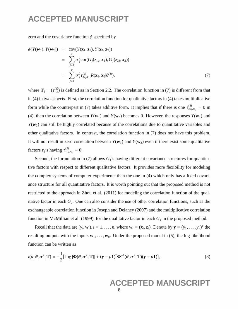
zero and the covariance functionφ specified by

φ(Y(w1),Y(w2)) = cov(Y(x1, z1),Y(x2, z2))

=

q∑

j=1

σ2j cor(Gj(z1 j , x1),Gj(z2 j , x2))

=

q∑

j=1

σ2jτ

( j)z1 j ,z2 j

R(x1, x2|θ( j)), (7)

whereT j = (τ( j)r,s) is defined as in Section 2.2. The correlation function in (7) is different from that

in (4) in two aspects. First, the correlation function for qualitative factors in (4) takes multiplicative

form while the counterpart in (7) takes additive form. It implies that if there is oneτ( j)z1 j ,z2 j = 0 in

(4), then the correlation betweenY(w1) andY(w2) becomes 0. However, the responsesY(w1) and

Y(w2) can still be highly correlated because of the correlations due to quantitative variables and

other qualitative factors. In contrast, the correlation function in (7) does not have this problem.

It will not result in zero correlation betweenY(w1) andY(w2) even if there exist some qualitative

factorszj ’s havingτ( j)z1 j ,z2 j = 0.

Second, the formulation in (7) allowsGj ’s having different covariance structures for quantita-

tive factors with respect to different qualitative factors. It provides more flexibility for modeling

the complex systems of computer experiments than the one in (4) which only has a fixed covari-

ance structure for all quantitative factors. It is worth pointing out that the proposed method is not

restricted to the approach in Zhou et al. (2011) for modeling the correlation function of the qual-

itative factor in eachGj. One can also consider the use of other correlation functions, such as the

exchangeable correlation function in Joseph and Delaney (2007) and the multiplicative correlation

function in McMillian et al. (1999), for the qualitative factor in eachGj in the proposed method.

Recall that the data are (yi ,wi), i = 1, . . . , n, wherewi = (xi , zi). Denote byy = (y1, . . . , yn)T the

resulting outputs with the inputsw1, . . . ,wn. Under the proposed model in (5), the log-likelihood

function can be written as

l(μ, θ,σ2,T) = −12[log |Φ(θ,σ2,T)| + (y − μ1)TΦ−1(θ,σ2,T)(y − μ1)

], (8)


ACCEPTED MANUSCRIPT

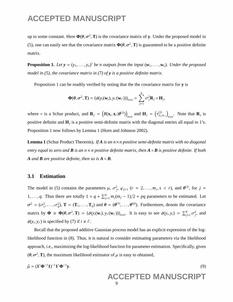
up to some constant. HereΦ(θ,σ2,T) is the covariance matrix ofy. Under the proposed model in

(5), one can easily see that the covariance matrixΦ(θ,σ2,T) is guaranteed to be a positive definite

matrix.

Proposition 1. Let y = (y1, . . . , yn)T be n outputs from the input(w1, . . . ,wn). Under the proposed

model in (5), the covariance matrix in (7) ofy is a positive definite matrix.

Proposition 1 can be readily verified by noting that the the covariance matrix fory is

Φ(θ,σ2,T) =(φ(yi(wi), yi′(wi′))

)n×n =

q∑

j=1

σ2j R j ◦ H j ,

where◦ is a Schur product, andR j =(R(xi , xi′ |θ

( j)))

n×nand H j =

(τ

( j)zi j ,zi′ j

)

n×n. Note thatR j is

positive definite andH j is a positive semi-definite matrix with the diagonal entries all equal to 1’s.

Proposition 1 now follows by Lemma 1 (Horn and Johnson 2002).

Lemma 1 (Schur Product Theorem). If A is an n×n positive semi-definite matrix with no diagonal

entry equal to zero andB is an n× n positive definite matrix, thenA ◦B is positive definite. If both

A andB are positive definite, then so isA ◦ B.

3.1 Estimation

The model in (5) contains the parametersμ, σ2j , ϕ j,r,s (r = 2, . . . ,mj , s < r), andθ( j), for j =

1, . . . , q. Thus there are totally 1+ q +∑q

j=1 mj(mj − 1)/2 + pq parameters to be estimated. Let

σ2 = (σ21, . . . , σ

2q), T = (T1, . . . ,Tq) andθ = (θ(1), . . . , θ(q)). Furthermore, denote the covariance

matrix by Φ ≡ Φ(θ,σ2,T) =(φ(yi(wi), yi′(wi′))

)n×n. It is easy to seeφ(yi , yi) =

∑qj=1σ

2j , and

φ(yi , yi′) is specified by (7) ifi , i′.

Recall that the proposed additive Gaussian process model has an explicit expression of the log-

likelihood function in (8). Thus, it is natural to consider estimating parameters via the likelihood

approach, i.e., maximizing the log-likelihood function for parameter estimation. Specifically, given

(θ,σ2,T), the maximum likelihood estimator ofμ is easy to obtained,

μ = (1TΦ−11)−11TΦ−1y. (9)


ACCEPTED MANUSCRIPT

Substituting (9) into (8), we obtain that the maximum of (8) is

l(μ, θ,σ2,T) = −12[log |Φ| + (yTΦ−1y) − (1TΦ−11)−1(1TΦ−1y)2].

The estimators ofθ,σ2,T can be obtained as

[θ, σ2, T] = argmin log|Φ| + (yTΦ−1y) − (1TΦ−11)−1(1TΦ−1y)2. (10)

The minimization problem in (10) requiresϕ j,r,s ∈ (0, π) andσ j ≥ 0 for j = 1, . . . , q. It can be

solved using standard non-linear optimization algorithms in Matlab or R.

3.2 Prediction and Interpolation

The prediction of the proposed additive Gaussian process is similar to the prediction procedure in

(3) for the ordinary kriging. Specifically, the prediction ofy at a new locationw0 = (x0, z0) is the

condition mean, i.e.,

E(y(w0)|y1, . . . , yn) = μ + φ(w0)TΦ−1(θ,σ2,T)(y − μ1), (11)

whereφ(w0) = (φ(w0,w1), . . . , φ(w0,wn))T. Thus given the estimates ˆμ, θ, σ, T, we have the pre-

diction ofy at a new locationw0 is

y(w0) = μ + φ(w0)TΦ−1(θ, σ2, T)(y − μ1). (12)

For interpolation, it is straightforward to show that whenw0 = wi, the coefficientφ(w0)TΦ−1(θ, σ2, T)

in (12) is ann-dimensional vector with theith entry being 1 and otherwise 0. Thus, ˆy(w0) = yi,

achieving the property of interpolation.

Moreover, the single-stage predictor in (12) can be viewed as a sequential predictor. To

see this, letΦ j = σ2j R j ◦ H j, we haveΦ =

∑qj=1Φ j by Proposition 1. Correspondingly, let

φ j(w0) = σ2j R(w0,w|θ( j)) ◦ H0 j, whereR(w0,w|θ( j)) = (R(w0,w1|θ

( j)), . . . ,R(w0,wn|θ( j))T and

H0 j = (τ( j)z0 j ,z1 j , . . . , τ

( j)z0 j ,zn j)

T. We haveφ(w0) = φ1(w0) + ∙ ∙ ∙ + φq(w0). Therefore, the prediction

atw0 can be rewritten as

y(w0) = μ + (φ1(w0) + ∙ ∙ ∙ + φq(w0))T(

q∑

j=1

Φ j)−1(y − μ1), (13)


ACCEPTED MANUSCRIPT

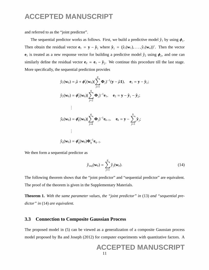
and referred to as the “joint predictor”.

The sequential predictor works as follows. First, we build a predictive model ˆy1 by usingφ1.

Then obtain the residual vectore1 = y − y1 where y1 = (y1(w1), . . . , y1(wn))T. Then the vector

e1 is treated as a new response vector for building a predictive model ˆy2 usingφ2, and one can

similarly define the residual vectore2 = e1 − y2. We continue this procedure till the last stage.

More specifically, the sequential prediction provides

y1(w0) = μ + φT1(w0)(

q∑

j=1

Φ j)−1(y − μ1), e1 = y − y1;

y2(w0) = φT2(w0)(

q∑

j=2

Φ j)−1e1, e2 = y − y1 − y2;

...

yk(w0) = φTk(w0)(

q∑

j=k

Φ j)−1ek−1, ek = y −

k∑

j=1

yj;

...

yq(w0) = φTq(w0)Φ

−1q eq−1.

We then form a sequential predictor as

yseq(w0) =q∑

j=1

yj(w0). (14)

The following theorem shows that the “joint predictor” and “sequential predictor” are equivalent.

The proof of the theorem is given in the Supplementary Materials.

Theorem 1. With the same parameter values, the “joint predictor” in(13) and “sequential pre-

dictor” in (14)are equivalent.

3.3 Connection to Composite Gaussian Process

The proposed model in (5) can be viewed as a generalization of a composite Gaussian process

model proposed by Ba and Joseph (2012) for computer experiments with quantitative factors. A


ACCEPTED MANUSCRIPT

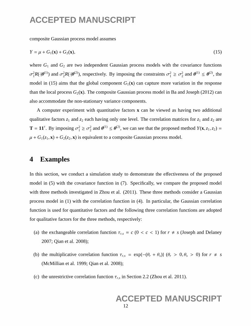
composite Gaussian process model assumes

Y = μ + G1(x) + G2(x), (15)

whereG1 andG2 are two independent Gaussian process models with the covariance functions

σ21R(∙|θ(1)) andσ2

2R(∙|θ(2)), respectively. By imposing the constraintsσ21 ≥ σ

22 andθ(1) ≤ θ(2), the

model in (15) aims that the global componentG1(x) can capture more variation in the response

than the local processG2(x). The composite Gaussian process model in Ba and Joseph (2012) can

also accommodate the non-stationary variance components.

A computer experiment with quantitative factorsx can be viewed as having two additional

qualitative factorsz1 andz2 each having only one level. The correlation matrices forz1 andz2 are

T = 11T. By imposingσ21 ≥ σ

22 andθ(1) ≤ θ(2), we can see that the proposed methodY(x, z1, z2) =

μ + G1(z1, x) + G2(z2, x) is equivalent to a composite Gaussian process model.

4 Examples

In this section, we conduct a simulation study to demonstrate the effectiveness of the proposed

model in (5) with the covariance function in (7). Specifically, we compare the proposed model

with three methods investigated in Zhou et al. (2011). These three methods consider a Gaussian

process model in (1) with the correlation function in (4). In particular, the Gaussian correlation

function is used for quantitative factors and the following three correlation functions are adopted

for qualitative factors for the three methods, respectively:

(a) the exchangeable correlation functionτr,s = c (0 < c < 1) for r , s (Joseph and Delaney

2007; Qian et al. 2008);

(b) the multiplicative correlation functionτr,s = exp{−(θr + θs)} (θr > 0, θs > 0) for r , s

(McMillian et al. 1999; Qian et al. 2008);

(c) the unrestrictive correlation functionτr,s in Section 2.2 (Zhou et al. 2011).


ACCEPTED MANUSCRIPT

Following the notation in Zhou et al. (2011), the three methods are denoted by ‘EC’, ‘MC’ and

‘UC’, respectively, while the proposed method is denoted by ‘AD UC’ as it adopts ‘UC’ for each

qualitative factors. Here we have not included Zhang and Notz (2015) for comparison, since their

method also adopts the multiplicity of correlations between quantitative and qualitative factors, in

a very similar spirit as that in Zhou et al. (2015). For the comparison purpose, we also include

the proposed additive Gaussian process model with EC and MC correlation structures for each

qualitative factor, denoted as ‘AD EC’ and ‘AD MC’, respectively.

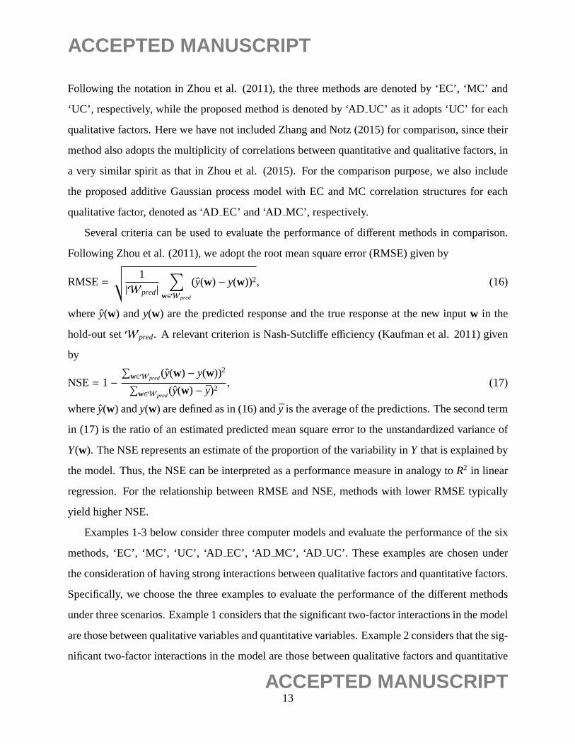
Several criteria can be used to evaluate the performance of different methods in comparison.

Following Zhou et al. (2011), we adopt the root mean square error (RMSE) given by

RMSE=

√√1

|Wpred|

∑

w∈Wpred

(y(w) − y(w))2, (16)

wherey(w) andy(w) are the predicted response and the true response at the new inputw in the

hold-out setWpred. A relevant criterion is Nash-Sutcliffe efficiency (Kaufman et al. 2011) given

by

NSE= 1−

∑w∈Wpred

(y(w) − y(w))2

∑w∈Wpred

(y(w) − y)2, (17)

wherey(w) andy(w) are defined as in (16) and ˉy is the average of the predictions. The second term

in (17) is the ratio of an estimated predicted mean square error to the unstandardized variance of

Y(w). The NSE represents an estimate of the proportion of the variability inY that is explained by

the model. Thus, the NSE can be interpreted as a performance measure in analogy toR2 in linear

regression. For the relationship between RMSE and NSE, methods with lower RMSE typically

yield higher NSE.

Examples 1-3 below consider three computer models and evaluate the performance of the six

methods, ‘EC’, ‘MC’, ‘UC’, ‘AD EC’, ‘AD MC’, ‘ AD UC’. These examples are chosen under

the consideration of having strong interactions between qualitative factors and quantitative factors.

Specifically, we choose the three examples to evaluate the performance of the different methods

under three scenarios. Example 1 considers that the significant two-factor interactions in the model

are those between qualitative variables and quantitative variables. Example 2 considers that the sig-

nificant two-factor interactions in the model are those between qualitative factors and quantitative


ACCEPTED MANUSCRIPT

variables as well as those between quantitative variables. Example 3 considers that the significant

two-factor interactions include interactions between quantitative variables, between quantitative

variable and qualitative variables, and between qualitative factors. In each example, we implement

the six methods over 100 simulations and report the associated RMSEs.

Example 1.Consider a computer experiment withp = 6 quantitative factors andq = 5 qualitative

factors each having three levels. Data are generated from the computer model

y =

5∑

i=1

xiz6−i

4000+

5∏

i=1

cos(xi√

i)sin(

z6−i√

i), (18)

where−100< xi < 100 for i = 1, . . . , p andzj = {−50,0,50} for j = 1, . . . , q. In each simulation,

a 81-run design is adopted, where a three-level fractional factorial design (Wu and Hamada 2009)

is used for qualitative factors and a random Latin hypercube design (McKay et al. 1979) is used

for quantitative factors. The RMSE in (16) is computed based on the hold-out setWpred with

2430 points consisting of four replicates of a full factorial three-level design for qualitative factors

and a random Latin hypercube design for quantitative factors. Figure 1 displays the boxplots

of the RMSEs associated with ‘EC’, ‘MC’, ‘UC’, ‘AD EC’, ‘AD MC’ and ‘AD UC’ for p =

6 over 100 simulations. From Figure 1, it is clearly seen that the proposed method ‘AD UC’

outperforms the other three methods since its corresponding RMSE is significantly lower than that

of the alternatives. Also the additive gaussian process methods ‘AD EC’, ‘AD MC’ and ‘AD UC’

perform better than ‘EC’, ‘MC’ and ‘UC’. It is noting that although the multiplicative correlation

model UC itself has relatively larger RMSE than EC and MC in this example, the ‘AD UC’ gets a

smaller RMSE than ‘AD EC’ and ‘AD MC’.

Example 2.Consider a computer experiment withp = 7 quantitative factors andq = 6 qualitative

factorsz1, . . . , z6, wherez1 andz2 have two levels,z3, z4 andz5 have three levels, andz6 has four

levels. Consider the computer model,

y =

5∑

i=1

exp{−xi}cos(4z7−i)sin(4xi+2) + exp{−x6}cos(4z1)sin(4z1)

+exp{−x7}cos(4x7)sin(4z2), (19)


ACCEPTED MANUSCRIPT

where 0< xi < 1 for i = 1, . . . , p, zj = {0.3,0.8} for j = 1,2, zj = {0.1,0.5,0.9} for j = 3,4,5

andzp+6 = {0.05,0.35,0.65,0.95}. In each simulation, an 142-run design is adopted, where two

replicates of a 72-run mixed-level fractional factorial design are used for qualitative factors and a

random Latin hypercube design is used for quantitative factors. The RMSE in (16) is computed

based on the hold-out setWpred with 2160 points consisting of five replicates of a full factorial de-

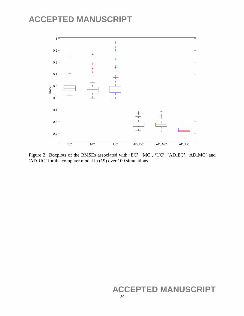
sign for qualitative factors and a random Latin hypercube design for quantitative factors. Figure 2

displays the boxplots of the RMSEs associated with ‘EC’, ‘MC’, ‘UC’, ‘AD’, ‘AD EC’, ‘AD MC’

and ‘AD UC’ over 100 simulations. The results in Figure 2 clearly indicate that the proposed

method ‘AD UC’ provides much lower RMSEs. One can also see that the prediction performances

of ‘EC’, ‘MC’, and ‘UC’ are very comparable in this example, while ‘AD UC’ is still relatively

better than ‘AD EC’ and ‘AD MC’ in terms of RMSE values.

Example 3.Consider the computer model,

y = 5g1(z5) + 3g2(z4) + 1.2g1(x4) + 1.5g2(x8) + 2.3g3(x2) + 7g2(x2)

+4g3(1.5z3 + x1) + 7g4(1.2z2 + x3) + 4.5g3(x9 + x6) (20)

+3g3(x4 + x5) + 1.1g2(z2 + z3) + 1.5g2(z1 + z5)

where 0< xi < 1 for i = 1, . . . , p, xj ∈ {0.1,0.5,0.9} for j = p + 1, . . . , k, g1(x) = x, g2(x) =

(2x−1)2, g3(x) = sin(2πx)/[2−sin(2πx)], andg4(x) = 0.1sin(2πx)+0.2cos(2πx)+0.3[sin(2πx)]2+

0.4[cos(2πx)]3 + 0.5[sin(2πx)]3. The functionsg1,g2,g3,g4 are defined in Reich, Storlie and Bon-

dell (2009). In each simulation, a three-level fractional factorial design of 81 runs is used for

qualitative factors and a random Latin hypercube design of 81 runs is used for quantitative factors.

The RMSE in (16) is computed based on the hold-out setWpred with 1215 points consisting of

five replicates of a full factorial design for qualitative factors and a random Latin hypercube design

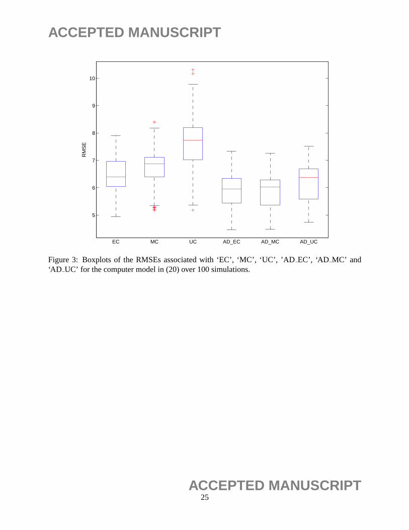
for quantitative factors. Figure 3 displays the boxplots of the RMSEs associated with ‘EC’, ‘MC’,

‘UC’, ‘ AD EC’, ‘AD MC’ and ‘AD UC’ for q = 5 andp = 9. The results show that the additive

Gaussian process methods ‘AD EC’, ‘AD MC’ and ‘AD UC’ still perform better than the other

three methods in comparison. However, the advantage of the additive Gaussian process methods

over the other three methods is not as significant as those in Examples 1-2. It is also worth noting


ACCEPTED MANUSCRIPT

that in this example, the advantage of the proposed method ‘AD UC’ is comparable to ‘AD EC’

and ‘AD MC’. One possible explanation is that the computer model in (20) does not have as strong

interactions between qualitative factors and quantitative factors as those in (18) and (19).

5 Real Data Analysis

In this section, we apply the proposed method to a real application in which the computer ex-

periment has both qualitative and quantitative factors. A fully 3D coupled finite element model

has been calibrated and verified by successfully capturing both the deformations and stresses of

full scale embankments involving unreinforced, piled, and two different reinforced and piled sec-

tions (Rowe and Liu 2015). Given the cost of building and monitoring full-scale reinforced and

column-supported embankment in field, a validated numerical modeling is usually regarded as a

cost-effective tool to advance the knowledge of complex issues in such a system involving geosyn-

thetic reinforced platform, embankment fill, columns, and geosynthetic reinforcement. In this

study, the aforementioned validated numerical model was used to investigate the influence of three

qualitative factors and one quantitative factor for improving the performance of reinforced em-

bankments with floating columns over soft clay. Figure 4 illustrates the structure of this full scale

embankment. A 7 meter (m) thick reinforced embankment was constructed over a 15 m soft clay

deposit improved with 1-m-diameter and 9-m-long columns at 2 m centre-to-centre spacing. The

finite element discretization for the case examined had 36,802 elements and 69,667 nodes (Fig-

ure 4a). The three qualitative factors are embankment construction rate (z1), Young’s modulus of

columns (z2), and reinforcement stiffness (z3), and the quantitative factorx1 is the distance from

the embankment centreline to the embankment shoulder (Figure 4b). An average run for one case

of this size took roughly 9 hours on a 12-noded parallel super-computer at the High Performance

Computing Virtual Laboratory (HPCVL). The response variable considered herein is the final em-

bankment crest settlementU3, which is a crucial embankment working indicator.

For the computer experiment, each of the three qualitative factorsz1, z2, z3 has three levels: the

levels ofz1 are 1, 5, 10 m/month; the levels ofz2 are 50, 100, 200 MPa; and the levels ofz3 are


ACCEPTED MANUSCRIPT

1578, 4800, 8000 kN/m. The quantitative factorx1 takes the 29 values uniformly from the interval

[0,14]. For each value of the quantitative factor, a three-level fractional factorial design of 9 runs

is used for the qualitative factors. Thus, there are 261 design points, which are used for model

estimation for the four methods ‘EC’, ‘MC’, ‘UC’ and ‘AD’, respectively.

To compare the prediction performance of these four methods, we evaluate their prediction

performance on the test data. Specifically, the test data set contains 29 input settings in which the

values of quantitative factorx1 are taken uniformly from the interval [0,14], and the setting of the

qualitative factors is (z1, z2, z3) = (5,100,4800). Note that such a setting of qualitative factors is

not used in the 9-run three-level fractional factorial design.

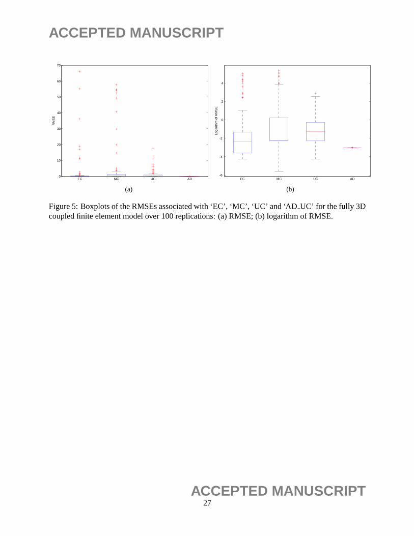
Figure 5 displays the boxplots of the RMSEs in (16) associated with ‘EC’, ‘MC’, ‘UC’ and

‘AD UC’ for the fully 3D coupled finite element model over 100 replications. From the boxplots

in the figure, one can clearly see that the proposed method performs much better than the other

three methods in terms of prediction accuracy and precision. It is worth pointing out that the RM-

SEs associated with ‘EC’, ‘MC’, ‘UC’ have large variations with a significant portion of outliers in

their boxplots. A possible explanation is that those methods have not full captured the underlying

correlation structures of qualitative and qualitative factors, resulting in large bias in the estimation

of the mean response. In addition, the proposed method gives nearly identical RMSEs over 100

replications because in this particular example the maximum likelihood estimates are found nearly

identical over those replications regardless the initial values of parameters in the maximum like-

lihood optimization. In summary for the case examined, the proposed ‘AD UC’ method presents

a very promising and time-saving tool to achieve excellent agreement with the computations from

complex computer experiments (i.e., fully 3D coupled finite element modeling).

6 Discussion

In this work, we propose an additive Gaussian process for modeling computer experiments with

both quantitative and qualitative factors. Several illustrative examples and a real application have

demonstrated that the proposed method can build a more accurate emulator comparing with the


ACCEPTED MANUSCRIPT

existing methods. The reason that might explain the success of the proposed method is that, the

proposed model employs a more flexible covariance structure that is capable of accommodating

the complex interaction effects between qualitative factors and quantitative factors.

A few remarks are worth mentioning here. First, the current work only considers the additive

Gaussian process with respect to the qualitative factors. There are several existing work consid-

ering additive kernels for the quantitative factors (Durrrande et al. 2010; Duvenaud et al. 2011).

How to incorporate additive kernels for the quantitative factors in our method can be an interest-

ing topic for future research. To extend the proposed method for accommodating the interactions

between qualitative factors, one possibility is to include those interactions in the mean part. By

conducting variable selection to include significant interactions in the mean part, the proposed

method deserves thorough investigations in the future work.

Second, the empirical study shows that the proposed method is particularly useful in building

Gaussian process modeling when the number of qualitative factors is relatively large, and the inter-

action effects between qualitative factors and quantitative factors are strong and complex. If instead

the number of qualitative factors is small and such interaction effects are not strong or complex, the

performance of the proposed method and other existing methods are likely to be very comparable.

It means that existing methods are probably sufficient in providing an accurate emulator. Third,

recall that the number of parameters in the proposed model is 1+ q+∑q

j=1 mj(mj − 1)/2+ pq, and

thus when the number of input variables and/or the levels of qualitative factors are large, parameter

estimation can be computationally cumbersome. There is a need for a computationally efficient es-

timation procedure. Finally, in a recent paper Deng, Hung, and Lin (2015) introduced marginally

coupled designs for computer experiments with both qualitative and quantitative factors. Ba et al.

(2015) proposed optimal sliced Latin hypercube designs paired with fractional factorial designs to

accommodate both qualitative and quantitative factors. Note that the space-filling property of a

design can have a significant impact on the model performance. It would be interesting to explore

the possibility of coupling the proposed model with those designs for more accurate emulators.


ACCEPTED MANUSCRIPT

Acknowledgements

The authors like to thank the Editor, the Associate Editor and two referees for their insightful

comments. Lin is supported by the Natural Sciences and Engineering Research Council of Canada.

Deng is supported by the National Science of Foundation of United States.


ACCEPTED MANUSCRIPT

References

Ba, S., and Joseph, V. R. (2012), “Composite Gaussian Process Models for Emulating Expensive

Functions,”The Annals of Applied Statistics, 6, 1838–1860.

Ba, S., Myers, W. R., and Brenneman, W. A. (2015). “Optimal Sliced Latin Hypercube Designs,”

Technometrics, 57, 479–487.

Bhuiyan, H., Chen, J., Khan, M., and Marathe, M. V. (2014), “Fast Parallel Algorithms for Edge-

Switching to Achieve a Target Visit Rate in Heterogeneous Graphs, ”In Parallel Processing

(ICPP), 2014 43rd International Conference on IEEE, 60–69.

Deng, X., Hung, Y., and Lin, C. D. (2015), “Design for Computer Experiments with Qualitative

and Quantitative Factors,”Statistica Sinica, to appear.

Durrande, N., Ginsbourger, D., Roustant, O., and Carraro, L. (2011), “Additive Covariance Ker-

nels for High-dimensional Gaussian Process Modeling,” arXiv preprint arXiv:1111.6233.

Duvenaud, D. K., Nickisch, H., and Rasmussen, C. E. (2011), “Additive Gaussian Processes,”

Advances in neural information processing systems, 226–234.

Fang, K. T., Li, R., and Sudjianto, A. (2005),Design and Modeling for Computer Experiments,

New York: Chapman&Hall/CRC Press.

Han, G., Santner, T. J., Notz, W. I., and Bartel, D. L. (2009), “Prediction for Computer Experi-

ments Having Quantitative and Qualitative Input Variables,”Technometrics, 51, 278–288.

Hastie, T. J., and Tibshirani, R. J. (1990),Generalized Additive Models, New York: CRC Press.

Horn, R. A., and Johnson, C. R. (2012),Matrix Analysis (Second Edition), New York: Cambridge

University Press.

Joseph, V. R., and Delaney, J. D. (2007), “Functionally Induced Priors for the Analysis of Exper-

iments, ”Technometrics, 49, 1–11.


ACCEPTED MANUSCRIPT

Kaufman, C. G., Bingham, D., Habib, S., Heitmann, K., and Frieman, J. A. (2011), “ Efficient

Emulators of Computer Experiments using Compactly Supported Correlation Functions,

with an Application to Cosmology,”The Annals of Applied Statistics, 5, 2470–2492.

Liu, K-W., and Rowe, R. K. (2015), “Numerical Study of the Effects of Geosynthetic Reinforce-

ment Viscosity on Behaviour of Embankments Supported by Deep-mixing-method (DMM)

Columns,”Geotextiles and Geomembranes, accepted.

Matern, B. (1986),Spatial Variation (Second Edition), New York: Springer-Verlag.

McKay, M. D., Beckman, R. J., and Conover, W. J. (1979), “A Comparison of Three Methods

for Selecting Values of Input Variables in the Analysis of Output from a Computer Code,”

Technometrics, 21, 239–45.

McMillian, N. J., Sacks, J., Welch, W. J., and Gao, F. (1999), “Analysis of Protein Activity Data

by Gaussian Stochastic Process Models,”Journal of Biopharmaceutical Statistics, 9, 145–

160.

Pinheiro, J. C., and Bates, D. M. (1996), “Unconstrained Parametrizations for Variance-Covariance

Matrices,”Statistics and Computing, 6, 289–296.

Qian, P. Z. G., Wu, H., and Wu, C. F. J. (2008), “Gaussian Process Models for Computer Experi-

ments With Qualitative and Quantitative Factors,”Technometrics, 50, 283–396.

Reich, B. J., Storlie, C. B., and Bondell, H. D. (2009), “Variable Selection in Bayesian Smoothing

Spline ANOVA Models: Application to Deterministic Computer Codes,”Technometrics, 51,

110–120.

Rowe, R. K., and Liu, K-W. (2015), “3D Finite Element Modeling of a Full-scale Geosynthetic-

Reinforced, Pile-supported Embankment,”Canadian Geotechnical Journal, accepted.

Rebonato, R., and Jackel, P. (1999), “The Most General Methodology for Creating a Valid Cor-

relation Matrix for Risk Management and Option Pricing Purposes,”The Journal of Risk, 2,

17–27.


ACCEPTED MANUSCRIPT

Swiler, L. P., Hough, P. D., Qian, P., Xu, X., Storlie, C., and Lee, H. (2014), “Surrogate Models for

Mixed Discrete-Continuous Variables,”In Constraint Programming and Decision Making

(pp. 181–202). Springer International Publishing.

Santner, T.J., Williams, B. J., and Notz, W. I. (2003),The Design and Analysis of Computer

Experiments. New York: Springer.

Sacks, J., Welch, W. J., Mitchell, T. J., and Wynn, H. P. (1989), “Design and Analysis of Computer

Experiments,”Statistical science, 409–423.

Wu, C. F. J., and Hamada, M. (2009),Experiments: Planning, Analysis, and Optimization, New

York: Wiley.

Zhang, Y., and Notz, W. I. (2015), “Computer Experiments with Qualitative and Quantitative

Variables: a Review and Reexamination,”Quality Engineering, 27, 2–13.

Zhou, Q., Qian, P. Z. G., and Zhou, S. (2011), “A Simple Approach to Emulation for Computer

Models With Qualitative and Quantitative Factors,”Technometrics, 53, 266–273.


ACCEPTED MANUSCRIPT

0.2

0.4

0.6

0.8

1

1.2

1.4

1.6

1.8

EC MC UC AD_EC AD_MC AD_UC

RM

SE

Figure 1: Boxplots of RMSEs associated with ‘EC’, ‘MC’, ‘UC’,’AD EC’, ‘ AD MC’ and‘AD UC’ for the computer model in (18) withp = 6 over 100 simulations.


ACCEPTED MANUSCRIPT

0.2

0.3

0.4

0.5

0.6

0.7

0.8

0.9

1


RM

SE

Figure 2: Boxplots of the RMSEs associated with ‘EC’, ‘MC’, ‘UC’,’AD EC’, ‘ AD MC’ and‘AD UC’ for the computer model in (19) over 100 simulations.


ACCEPTED MANUSCRIPT

5

6

7

8

9

10


RM

SE

Figure 3: Boxplots of the RMSEs associated with ‘EC’, ‘MC’, ‘UC’,’AD EC’, ‘ AD MC’ and‘AD UC’ for the computer model in (20) over 100 simulations.


ACCEPTED MANUSCRIPT

Figure 4: The embankment examined: (a) finite element mesh; (b) the schematic view of embank-ment constructed on foundation soil.


ACCEPTED MANUSCRIPT

0

10

20

30

40

50

60

70

EC MC UC AD

RM

SE

(a)

-6

-4

-2

0

2

4

EC MC UC AD

Loga

rithm

of R

MS

E

(b)

Figure 5: Boxplots of the RMSEs associated with ‘EC’, ‘MC’, ‘UC’ and ‘AD UC’ for the fully 3Dcoupled finite element model over 100 replications: (a) RMSE; (b) logarithm of RMSE.


Documents

ACCEPTED MANUSCRIPT - Virginia Tech · · 2016-10-12ACCEPTED MANUSCRIPT Additive Gaussian Process for Computer Models With Qualitative and Quantitative Factors X. Deng†, C. Devon