ACCEP

TED M

ANUSC

RIPT

ACCEPTED MANUSCRIPT

Temporal Reasoning about Fuzzy Intervals

Steven Schockaert ∗,1, Martine De Cock

Ghent University, Department of Applied Mathematics and Computer Science,Krijgslaan 281 - S9, 9000 Gent, Belgium

Abstract

Traditional approaches to temporal reasoning assume that time periods and timespans of events can be accurately represented as intervals. Real–world time pe-riods and events, on the other hand, are often characterized by vague temporalboundaries, requiring appropriate generalizations of existing formalisms. This paperpresents a framework for reasoning about qualitative and metric temporal relationsbetween vague time periods. In particular, we show how several interesting prob-lems, like consistency and entailment checking, can be reduced to reasoning tasksin existing temporal reasoning frameworks. We furthermore demonstrate that allreasoning tasks of interest are NP–complete, which reveals that adding vaguenessto temporal reasoning does not increase its computational complexity. To supportefficient reasoning, a large tractable subfragment is identified, among others, gener-alizing the well–known ORD Horn subfragment of the Interval Algebra (extendedwith metric constraints).

Key words: Temporal Reasoning, Interval Algebra, Fuzzy Set Theory

1 Introduction

Time plays a key role in many application domains, ranging from schedul-ing and planning [2,17,19] to natural language understanding [29,34], multi–document summarization [6], question answering [39,32,22] and dynamic mul-timedia presentation [3,10,18]. Starting from Allen’s seminal work on quali-tative interval relations (e.g., A happened during B, A overlaps with B; [1]),increasingly more expressive formalisms have been proposed to reason about

∗ Corresponding author.Email addresses: Steven.Schockaert@UGent.be (Steven Schockaert),

Martine.DeCock@UGent.be (Martine De Cock).1 Research Assistant of the Research Foundation – Flanders.

Preprint submitted to Elsevier 14 December 2007

ACCEP

TED M

ANUSC

RIPT

ACCEPTED MANUSCRIPT

time, among others allowing to specify metric constraints between two timepoints (e.g., p happened 4 time units before q; [12]), to combine qualitativeand metric information [25,31], to specify constraints on the (relative) dura-tion of events [35], and to specify arbitrary disjunctions of temporal constraints[23,27]. Most reasoning tasks of interest in these formalisms are NP–complete.To cope with this, a lot of research efforts have been directed towards identify-ing subfragments of the various calculi in which reasoning becomes tractable[13,14,28,37], as well as towards deriving efficient solution strategies for NP–complete reasoning problems [8,36,45,46].

Research, however, has largely focused on reasoning about time periods, andtime spans of events, which can be accurately represented as an interval. Incontrast, many real–world events and time periods are characterized by aninherently gradual or ill–defined beginning and ending. Typical examples arelarge–scale historical events like the Russian Revolution, the Great Depression,the Second World War, the Cold War, and the Dotcom Bubble, or historicaltime periods like the Middle Ages, the Renaissance, the Age of Enlighten-ment, and the Industrial Revolution, but also small-scale events like sleepingand being born. Moreover, in natural language, vague temporal markers arefrequently found to convey underspecified temporal information: early sum-mer, during his childhood, in the evening, etc. Note that the vagueness of theseevents and time periods is fundamentally different from the uncertainty thatexists among historicians about, for example, the time period during whichthe Mona Lisa was painted.

A formal definition of the notion of an event is difficult to provide. Clearly,an event is something that happens at a particular time and a particularplace (e.g., World War II); it can have parts (e.g., the Battle of the Bulge),it can belong to a certain category (e.g., Military Conflict) and it can haveconsequences (e.g., the Cold War) [47]. We will, however, abstract away fromany particular formalization of events, and focus on their temporal dimensiononly. As such, we will conceptually make no difference between time periodsand events. Vague time periods are naturally represented as fuzzy sets [48]. Avague time period is then represented as a mapping A from the real line R tothe unit interval [0, 1]. For a time instant t (t ∈ R), A(t) expresses to whatextent t belongs to the time period A. When A is a crisp time period, for all t inR, A(t) is either 0 (perfect non-membership) or 1 (perfect membership). WhenA is a vague time period, on the other hand, A will typically be graduallyincreasing over an interval [t1, t2] and gradually decreasing over an interval[t3, t4], where A(t) = 1 for t in [t2, t3] and A(t) = 0 for t < t1 and t > t4. Asan example, consider Picasso’s Blue, Rose and Cubist periods. Regarding thedefinition of the Rose period, for example, we find 2

2 http://pablo-picasso.paintings.name/rose-period/, accessed May 21,2007

2

ACCEP

TED M

ANUSC

RIPT

ACCEPTED MANUSCRIPT

Fig. 1. Fuzzy sets defining the vague time span of Picasso’s Blue, Rose, and Cubistperiods.

So 1904 is a transitional year and belongs neither truly to the blue period,nor to the rose period.

Similarly, the ending of the Rose period, as well as the beginning and ending ofthe Cubist period are inherently gradual. Figure 1 depicts a possible definitionof Picasso’s Rose period, as well as the ending of his Blue period and thebeginning of his Cubist period. These definitions reflect the gradual transitionto the Rose period during 1904, as well as Picasso’s experiments with newstyles from 1906 and especially from 1907, eventually leading to his Cubistperiod. Clearly, the definition of a fuzzy set representing a vague time periodis to some extent subjective. In fact, there is no real reason why January 1,1907 should belong to the Rose period to degree 0.8 and not to degree 0.75or 0.85. What is most important is the qualitative ordering the membershipdegrees impose, e.g., June 1, 1907 is more compatible with the Rose periodthan the Cubist period; March 15, 1904 is less compatible with the Rose periodthan June 1, 1907, etc.

Applications based on classical temporal reasoning algorithms, like temporalquestion answering or multi–document summarization, fail to work correctlywhen the events or time periods involved are vague. For example, when ex-tracting information about the life and work of Picasso from web documents,inconsistencies quickly arise:

(1) Bread and Fruit Dish on a Table (1909) marks the beginning of Picasso’s“Analytical” Cubism . . . 3

(2) The first stage of Picasso’s cubism is known as analytical cubism. It beganin 1908 and ended in 1912, . . . 4

3 http://www.abcgallery.com/P/picasso/picassobio.html, accessed May 21,20074 http://www.pokemonultimate.wanadoo.co.uk/picasso.html, accessed May21, 2007

3

ACCEP

TED M

ANUSC

RIPT

ACCEPTED MANUSCRIPT

(3) The ‘Demoiselles d’Avignon’ of 1907 mark the beginning of his [Picasso’s]Cubist period in which he exceeded the classical form. 5

The solution to this problem is not to discard the least reliable sources un-til the resulting knowledge base is consistent, but to acknowledge that someof the temporal relations expressed in the sentences above are only true tosome extent: the beginning of Picasso’s Analytical Cubism coincides with thebeginning of cubism to some degree λ1, Picasso’s Cubist period began with“Demoiselles d’Avignon” in 1907 to some degree λ2, Picasso’s Analytical Cu-bism began in 1908 to some degree λ3, Picasso’s Analytical Cubism began with“Bread and Fruit Dish on a Table” in 1909 to some degree λ4. The aim of thispaper is to derive algorithms for reasoning about such fuzzy temporal infor-mation, e.g., which values of λ1, λ2, λ3, λ4 result in a consistent interpretationof the sentences above? What conclusions can we establish given a consistentset of (fuzzy) assertions about (vague) time periods? Our primary objective isto obtain a temporal reasoning framework that is, among others, suitable fornatural language applications like multi–document summarization or questionanswering when some of the time periods and events involved are vague.

The structure of this paper is as follows. In the next section, we review relatedwork on fuzzy temporal information processing, while Section 3 familiarizesthe reader with some important preliminaries from fuzzy set theory and tem-poral reasoning. In Section 4, we introduce our framework for representingfuzzy temporal information. Next, in Section 5, we introduce an algorithm tocheck the consistency of a set of assertions about fuzzy time periods. The com-putational complexity of this problem is investigated in Section 6. Section 7discusses how new information can be derived from given information. Finally,Section 8 presents some concluding remarks and directions for future work.

2 Related work

Although processing fuzzy temporal information is well studied in literature,research has tended to focus on modelling vague temporal information aboutcrisp events (e.g., Picasso died in the early 1970s), rather than on modellingtemporal information about vague events. For example, in [16] possibility the-ory is employed to represent vague dates (e.g., early summer), and vaguetemporal constraints (e.g., A happened about three months before B). Theunderlying assumption is that all events have crisp, albeit unknown, temporalboundaries; only our knowledge about these crisp boundaries is vague. Basedon this possibilistic approach, [5] introduced the notion of a fuzzy temporal

5 http://www.kettererkunst.com/details-e.php?obnr=410702527&anummer=315, accessed May 21, 2007

4

ACCEP

TED M

ANUSC

RIPT

ACCEPTED MANUSCRIPT

constraint network. In this framework, temporal information is representedas fuzzy temporal constraints, i.e., fuzzy restrictions on the possible distancesbetween time points. Sound and complete reasoning procedures were providedin [30]. A generalization in which disjunctions of fuzzy temporal constraintscan be expressed has been introduced in [8].

A different line of research has focused on fuzzy extensions of classical calculifor temporal reasoning to encode preferences. For example, [26] discusses ageneralization of Temporal Constraint Satisfaction Problems (TCSP) in whicha preference value is attached to each temporal constraint. When a given TCSPis inconsistent, the preference values are used to determine which constraintsshould be ignored. Similarly, [4] introduces the framework IAfuz in whichpreference values are attached to atomic Allen relations. A relation in IAfuz

can thus be regarded as a fuzzy set of atomic Allen relations. Interestingly, allmain reasoning tasks are shown to be NP–complete and a maximal tractablesubfragment is identified. Fuzzy sets of atomic Allen relations have also beenconsidered in [21], where the adequate modelling of temporal expressions innatural language was the main motivation, rather than encoding preferences.

The need for formalisms dealing with vague events and time periods has beenpointed out in various contexts, including semantic web reasoning [9], his-torical databases and ontologies [33], document retrieval [24], and temporalquestion answering [40]. Nevertheless, none of the approaches mentioned aboveis suitable to represent temporal information about events whose boundariesare inherently gradual or ill–defined. Inspired by measures for comparing andranking fuzzy numbers [7,15], some definitions of fuzzy temporal relations be-tween vague events have already been proposed [33,38,42]. A key problem ingeneralizing temporal relations to cope with fuzzy time spans is that tradition-ally, temporal relations have been defined as constraints on boundary pointsof intervals. Because such well–defined boundary points are absent in fuzzytime intervals, alternative ways of looking at temporal relations are required.

Nagypal and Motik [33] start from the observation that several sets of timepoints can be associated with each interval A = [a−, a+], viz. the semi–intervals A<− =] − ∞, a−[, A≤− =] − ∞, a−], A<+ =] − ∞, a+[, A≤+ =] − ∞, a+], A>− =]a−, +∞[, A≥− = [a−, +∞[, A>+ =]a+, +∞[ and A≥+ =[a+, +∞[. Qualitative constraints on the boundary points of two intervalsA = [a−, a+] and B = [b−, b+] can be translated into set operations on thecorresponding semi–intervals. For example, m(A, B) holds iff a+ = b−, whichcan be expressed as A>+ ∩ B<− = ∅ ∧ A<+ ∩ B>− = ∅. To define qualita-tive temporal relations between fuzzy time spans, Nagypal and Motik defineA<−, A≤−, A<+, A≤+, A>−, A≥−, A>+, A≥+ for a fuzzy set A as:

A>−(p) = supq<p

A(q) A≤−(p) = 1 − A>−(p)

5

ACCEP

TED M

ANUSC

RIPT

ACCEPTED MANUSCRIPT

A≥−(p) = supq≤p

A(q) A<−(p) = 1 − A≥−(p)

A<+(p) = supq>p

A(q) A≥+(p) = 1 − A<+(p)

A≤+(p) = supq≥p

A(q) A>+(p) = 1 − A≤+(p)

The degree to which m(A, B) is satisfied, for instance, is then defined as

m(A, B) = min(1 − supp∈R

min(A>+(p), B<−(p)), 1 − supp∈R

min(A<+(p), B>−(p)))

= min(infp∈R

max(1 − A>+(p), 1 − B<−(p)),

infp∈R

max(1 − A<+(p), 1 − B>−(p)))

= min(infp∈R

max(A≤+(p), B≥−(p)), infp∈R

max(A≥+(p), B≤−(p)))

Although this approach has a certain appeal, the resulting fuzzy temporalrelations do not always behave intuitively. For example, for crisp intervals theequals relation is reflexive, while starts, finishes and during are irreflexive.Taking into account this intended meaning, we would expect that for fuzzytime spans e(A, A) = 1 and s(A, A) = f(A, A) = d(A, A) = 0, or at least,that e(A, A) > max(s(A, A), f(A, A), d(A, A)). However, using the definitionsproposed by Nagypal and Motik, if A is a continuous fuzzy set, it holds thate(A, A) = s(A, A) = f(A, A) = d(A, A) = 0.5. The reason for this anomaly liesin the definition of the fuzzy sets A<−, A≤−, . . . , A≥+. While these definitionsdo correspond to their intended meaning when A is a crisp interval, for acontinuous fuzzy set A, we have the undesirable property that A>− = A≥−,A<− = A≤−, A>+ = A≥+ and A<+ = A≤+.

In [38], a fundamentally different approach to modelling temporal relationsbetween fuzzy time spans is taken. The starting point is that even for crispintervals A and B, relations like before can hold to some degree. For example,if A = [0, 50] and B = [45, 100], we may intuitively think of A as being beforeB, instead of overlapping with B, because most of A is before the beginningof B. In [38], the degree to which b(A, B) holds is therefore defined basedon which fraction of A is before the beginning of B, where A and B may becrisp or fuzzy time spans. When temporal relations are defined in this way,we (deliberately) lose the original meaning of Allen’s relations. Although suchdefinitions may definitely be useful in many domains (e.g., querying temporaldatabases), they are not suitable as a basis for fuzzy temporal reasoning.

To the best of our knowledge, however, the issue of temporal reasoning aboutfuzzy time intervals has only been addressed in [40], where a sound but incom-plete algorithm is introduced to find consequences of a given, restricted set ofassertions. Finally, note that this paper is an extended and generalized versionof [43]. In addition to providing a more detailed discussion, as well as proofsof all results, we generalize the results from [43], where a purely qualitative

6

ACCEP

TED M

ANUSC

RIPT

ACCEPTED MANUSCRIPT

approach was adopted, by also considering metric constraints.

3 Preliminaries

3.1 Fuzzy temporal relations

A fuzzy set [48] in a universe U is defined as a mapping A from U to [0, 1],representing a vague concept. For u in U , A(u) expresses the degree to whichu is compatible with the concept A and is called the membership degree ofu in A. In particular, we will use fuzzy sets in R to represent time spans ofvague events. For clarity, traditional sets are sometimes called crisp sets in thecontext of fuzzy set theory. If A and B are fuzzy sets in the same universe U ,A is called a fuzzy subset of B, written A ⊆ B, iff A(u) ≤ B(u) for all u in U .

For every α in ]0, 1], we let Aα denote the crisp subset of U defined by

Aα = {u|u ∈ U ∧ A(u) ≥ α}

Aα is called the α–level set of the fuzzy set A. In particular, A1 is the set ofelements from U that are fully compatible with the vague concept modelledby A. If A1 �= ∅, the fuzzy set A is called normalised and elements from A1

are called modal values of A. The support supp(A) of A is the (crisp) set ofelements from U which belong to A to a strictly positive degree:

supp(A) = {u|u ∈ U ∧ A(u) > 0}

A fuzzy set A in R is called convex if for every α in ]0, 1], the set Aα is convex(i.e., a singleton or an interval).

To adequately generalize the notion of a time interval, a closed and boundedinterval of real numbers, some natural restrictions on the α–level sets aretypically imposed.Definition 1 (Fuzzy time interval). [42] A fuzzy (time) interval is a nor-malised fuzzy set in R with a bounded support, such that for every α in ]0, 1],Aα is a closed interval.

For example, the fuzzy sets corresponding to Picasso’s Blue, Rose and Cubistperiod from Figure 1 are fuzzy time intervals. The condition that all α–levelsets of a fuzzy time span be intervals implies that any fuzzy time intervalis a convex fuzzy set in R. Hence, fuzzy time intervals always consist of amonotonically increasing part, followed by a monotonically decreasing part.As a consequence, the fuzzy set depicted in Figure 2(a) is a fuzzy time span,whereas the fuzzy set from 2(b) is not, because of the decreasing part between

7

ACCEP

TED M

ANUSC

RIPT

ACCEPTED MANUSCRIPT

(a) (b)

(c) (d)

Fig. 2. The fuzzy sets of real numbers displayed in (a) and (c) are fuzzy time spans,whereas those in (b) and (d) are not.

a and b. By furthermore requiring that α–level sets be closed sets, we restrictthe kind of discontinuities allowed. For example, the fuzzy set from Figure2(d) is not a fuzzy time interval, since its 0.4– and 0.7–level sets are half openintervals. On the other hand, the fuzzy set shown in Figure 2(c) is a fuzzytime interval. It can be shown that a bounded fuzzy set of real numbers isa fuzzy time interval iff it is convex and upper semi–continuous. For a fuzzyinterval A and α ∈]0, 1], we let A−

α and A+α denote the beginning and ending

of the interval Aα.

When the time spans of events are vague, also the temporal relations betweenthem are a matter of degree. Traditionally, temporal relations between timeintervals have been defined by means of constraints on the boundary pointsof these intervals. Due to the gradual nature of fuzzy time spans, a different,more general approach has to be adopted here. The definitions of our fuzzytemporal relations are inspired by the fact that temporal relations betweentime intervals can alternatively be specified using first-order expressions thatdo not involve any boundary points. For example, for crisp intervals A =[a−, a+] and B = [b−, b+], it is easy to see that (d ∈ R)

a− < b− − d ⇔ (∃p)(p ∈ A ∧ (∀q)(q ∈ B ⇒ p < q − d)) (1)

To define the degree to which the beginning of a fuzzy time interval A is morethan d time units before the beginning of B, written bb�d (A, B), we gener-alize the right-hand side of (1) using fuzzy logic connectives. In fuzzy logic,elements from the unit interval [0, 1] represent truth degrees. To generalizelogical conjunction to fuzzy logic, a wide class of [0, 1]2 − [0, 1] mappings,

8

ACCEP

TED M

ANUSC

RIPT

ACCEPTED MANUSCRIPT

t-norm residual implicator

TM (x, y) = min(x, y) ITM(x, y) =

{1 if x ≤ y

y otherwise

TP (x, y) = x · y ITP(x, y) =

{1 if x ≤ yyx otherwise

TW (x, y) = max(0, x + y − 1) ITW(x, y) = min(1, 1 − x + y)

Table 1Commonly used t-norms and their residual implicators.

called t-norms, can be used. The only requirements are that the mapping Tbeing used is symmetric, associative, increasing, and satisfies the boundarycondition T (x, 1) = x for all x in [0, 1]. Logical implication can be generalizedusing the residual implicator IT of a t-norm T , i.e. the [0, 1]2 − [0, 1] mappingdefined for x and y in [0, 1] as

IT (x, y) = sup{λ|λ ∈ [0, 1] ∧ T (x, λ) ≤ y}

Some commonly used t-norms are the minimum TM , the product TP andthe �Lukasiewicz t-norm TW . Their definitions and the corresponding residualimplicators are displayed in Table 1. Universal and existential quantificationcan be generalized using the infimum and supremum respectively.

This leads to the following definition [42]:

bb�d (A, B) = supp∈R

T (A(p), infq∈R

IT (B(q), L�d (p, q))) (2)

where L�d (p, q) = 1 iff p < q − d and L�

d (x, y) = 0 otherwise. In the sameway, we can define the degree ee�d (A, B) to which the end of A is more than dtime units before the end of B, the degree be�d (A, B) to which the beginningof A is more than d time units before the end of B and the degree eb�(A, B)to which the end of A is more than d time units before the beginning of B as[42]:

ee�d (A, B) = supq∈R

T (B(q), infp∈R

IT (A(p), L�d (p, q))) (3)

be�d (A, B) = supp∈R

T (A(p), supq∈R

T (B(q), L�d (p, q))) (4)

eb�d (A, B) = infp∈R

IT (A(p), infq∈R

IT (B(q), L�d (p, q))) (5)

Finally, the degree bb�d (A, B) to which the beginning of A is at most d time

units after the beginning of B is defined by

bb�d (A, B) = 1 − bb�d (B, A) (6)

9

ACCEP

TED M

ANUSC

RIPT

ACCEPTED MANUSCRIPT

Table 2Characterization of the fuzzy temporal relations when A and B correspond to crispintervals [a−, a+] and [b−, b+].

Fuzzy Crisp Fuzzy Crisp

bb�d (A,B) a− < b− − d bb�d (A,B) a− ≤ b− + d

ee�d (A,B) a+ < b+ − d ee�d (A,B) a+ ≤ b+ + d

be�d (A,B) a− < b+ − d be�d (A,B) a− ≤ b+ + d

eb�d (A,B) a+ < b− − d eb�d (A,B) a+ ≤ b− + d

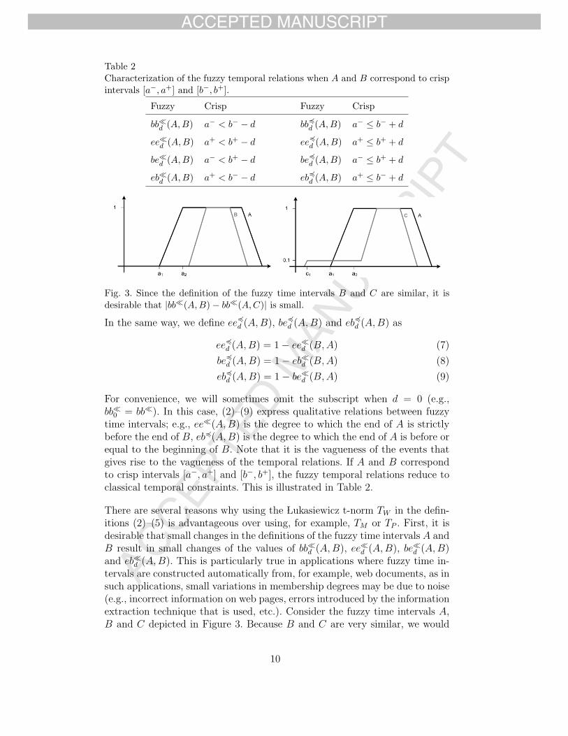
Fig. 3. Since the definition of the fuzzy time intervals B and C are similar, it isdesirable that |bb�(A,B) − bb�(A,C)| is small.

In the same way, we define ee�d (A, B), be�

d (A, B) and eb�d (A, B) as

ee�d (A, B) = 1 − ee�d (B, A) (7)

be�d (A, B) = 1 − eb�d (B, A) (8)

eb�d (A, B) = 1 − be�d (B, A) (9)

For convenience, we will sometimes omit the subscript when d = 0 (e.g.,bb�0 = bb�). In this case, (2)–(9) express qualitative relations between fuzzytime intervals; e.g., ee�(A, B) is the degree to which the end of A is strictlybefore the end of B, eb�(A, B) is the degree to which the end of A is before orequal to the beginning of B. Note that it is the vagueness of the events thatgives rise to the vagueness of the temporal relations. If A and B correspondto crisp intervals [a−, a+] and [b−, b+], the fuzzy temporal relations reduce toclassical temporal constraints. This is illustrated in Table 2.

There are several reasons why using the �Lukasiewicz t-norm TW in the defin-itions (2)–(5) is advantageous over using, for example, TM or TP . First, it isdesirable that small changes in the definitions of the fuzzy time intervals A andB result in small changes of the values of bb�d (A, B), ee�d (A, B), be�d (A, B)and eb�d (A, B). This is particularly true in applications where fuzzy time in-tervals are constructed automatically from, for example, web documents, as insuch applications, small variations in membership degrees may be due to noise(e.g., incorrect information on web pages, errors introduced by the informationextraction technique that is used, etc.). Consider the fuzzy time intervals A,B and C depicted in Figure 3. Because B and C are very similar, we would

10

ACCEP

TED M

ANUSC

RIPT

ACCEPTED MANUSCRIPT

Fig. 4. The generalized transitivity rule (11) may be violated when TM or TP isused.

like to have that the value of bb�(A, B) is close to the value of bb�(A, C).Irrespective of the t-norm T being used, it holds that bb�(A, B) = 1, i.e., thebeginning of A is strictly before the beginning of B to degree 1. When usingTM , however, we have that

bb�(A, C) = supp∈R

TM(A(p), infq∈R

ITM(C(q), L�(p, q)))

≤ supp∈R

TM(A(p), ITM(C(c1), L

�(p, c1)))

where c1 is defined as in Figure 3. As for each p in R either A(p) = 0 orL�(p, c1) = 0, we establish that bb�(A, C) = 0. In the same way, we can showthat bb�(A, C) = 0 when using TP . On the other hand, when T = TW , we canshow that

bb�(A, C) = supp∈R

TW (A(p), infq∈R

ITW(C(q), L�(p, q)))

= TW (A(a2), ITW(C(c1), L

�(a2, c1)))

= ITW(0.1, 0)

= 0.9

Another advantage of the �Lukasiewicz t-norm is related to transitivity. Toensure that the fuzzy temporal relations (2)–(9) display an intuitive behaviour,it is desirable that they satisfy generalized transitivity rules like

T (bb�(A, B), bb�(B, C)) ≤ bb�(A, C) (10)

T (bb�(A, B), bb�(B, C)) ≤ bb�(A, C) (11)

expressing that the degree to which the beginning of A is (strictly) before thebeginning of C is at least as high as the degree to which both the beginningof A is (strictly) before the beginning of B and the beginning of B is (strictly)before the beginning of C. While it is possible to show that (10) holds forany left-continuous t-norm (i.e., a t-norm whose partial mappings are left-continuous, such as TM , TP and TW ), (11) may be violated when TM or TP isused. For example, let A, B and C be defined as in Figure 4. Regardless of

11

ACCEP

TED M

ANUSC

RIPT

ACCEPTED MANUSCRIPT

whether T is TM , TP or TW , it holds that

bb�(A, B) = bb�(B, C) = 0.5

bb�(A, C) = 1

This implies

TM(bb�(C, B), bb�(B, A))

= min(1 − bb�(B, C), 1 − bb�(A, B))

= 0.5

> bb�(C, A) = 0

violating (11). In the same way, we find

TP (bb�(C, B), bb�(B, A)) = 0.25 > bb�(C, A) = 0

As shown in [41], all generalized transitivity rules of interest are satisfied whenthe �Lukasiewicz t-norm is used. Although we can use alternative definitions forbb�

d , ee�d , be�

d and eb�d for which the generalized transitivity rules are satisfied

for any left-continuous t-norm, we would then lose the important propertythat bb�d (A, B) = 1 − bb�

d (B, A), ee�d (A, B) = 1 − ee�d (B, A), etc. We refer

to [41] for more details. Henceforth, we will always assume that T = TW . Forconvenience, we will write IW instead of ITW

.

Finally, we show two characterizations which will be useful for solving thesatisfiability problem in Section 5.Lemma 1. It holds that

bb�d (A, B) ≥ l ⇔ (∀ε ∈]0, l])(∃λ ∈]l − ε, 1])(bb�d (Aλ, Bλ+ε−l)) (12)

bb�d (A, B) ≤ k ⇔ (∀λ ∈]k, 1])(bb�d (Bλ−k, Aλ)) (13)

ee�d (A, B) ≥ l ⇔ (∀ε ∈]0, l])(∃λ ∈]l − ε, 1])(ee�d (Aλ+ε−l, Bλ)) (14)

ee�d (A, B) ≤ k ⇔ (∀λ ∈]k, 1])(ee�d (Bλ, Aλ−k)) (15)

be�d (A, B) ≥ l ⇔ (∀ε ∈]0, l[)(∃λ ∈ [l − ε, 1])(be�d (Aλ, B1−λ−ε+l)) (16)

be�d (A, B) ≤ k ⇔ (∀ε ∈]0, 1 − k[)(∀λ ∈ [k + ε, 1])(eb�d (B1−λ+ε+k, Aλ)) (17)

eb�d (A, B) ≥ l ⇔ (∀ε ∈]0, l])(∀λ ∈ [1 − l + ε, 1])(eb�d (A1−λ+ε+1−l, Bλ)) (18)

eb�d (A, B) ≤ k ⇔ (∃λ ∈ [1 − k, 1])(be�d (Bλ, A2−λ−k)) (19)

Proof. See Appendix A.1.

Lemma 2. Let A and B be normalised and convex fuzzy sets in R. Further-more, let ma and mb be arbitrary modal values of A and B respectively. It

12

ACCEP

TED M

ANUSC

RIPT

ACCEPTED MANUSCRIPT

holds that

bb�d (A, B) = supp+d<mb,p≤ma

TW (A(p), 1 − B(p + d)) (20)

ee�d (A, B) = supp−d>ma,p≥mb

TW (B(p), 1 − A(p − d)) (21)

Proof. See Appendix A.2.

3.2 Linear constraints

An atomic linear constraint over a set of variables X is an expression of theform a1x1+a2x2+· · ·+anxn � b where a1, a2, . . . , an, b ∈ R, x1, x2, . . . , xn ∈ X,and � is <,≤, >,≥, = or �=. If φ1, φ2, . . . , φm are atomic linear constraints overX, φ1 ∨ φ2 ∨ · · · ∨ φm is called a linear constraint over X. If m > 1, the linearconstraint is called disjunctive. Furthermore, φ1 ∨ φ2 ∨ · · · ∨ φm is called aHorn linear constraint if at least m − 1 of the disjuncts φi correspond to �=.In particular, all atomic linear constraints are Horn, as well as, for example,3x + 4y ≤ 6 ∨ x �= 8 ∨ y �= 7 ∨ x + 3y �= 12. On the other hand, a linearconstraint like 3x + 4y ≤ 6 ∨ x ≥ 8 is not Horn.

The framework of linear constraints subsumes most other frameworks for tem-poral reasoning, including the Interval Algebra [1] and Temporal ConstraintNetworks [12], but also, for example, approaches combining qualitative andquantitative information [31] or expressing constraints on the duration ofevents [35].

A P–interpretation I over X is a mapping that maps every variable x fromX to a real number. For convenience, I(x) will also we written as xI . Anatomic linear constraint a1x1 + a2x2 + · · · + anxn � b is satisfied by I iffa1x

I1 +a2x

I2 + · · ·+anx

In � b. A disjunctive linear constraint φ1 ∨φ2 ∨ · · · ∨φm

is satisfied by I iff I satisfies at least one of the disjuncts φ1, φ2, . . . , φm. LetΨ be a set of linear constraints; I is called a P–model of Ψ iff I satisfies everylinear constraint in Ψ. If a P–model of Ψ exists, Ψ is called P–satisfiable. It hasbeen shown independently in [23] and [27] that checking the P–satisfiabilityof a set of Horn linear constraints can be done in polynomial time.

4 Temporal relations between vague events

For A and B fuzzy time intervals, bb�d (A, B), bb�d (A, B), ee�d (A, B), ee�

d (A, B),be�d (A, B), be�

d (A, B), eb�d (A, B) and eb�d (A, B) take values from [0, 1] (d ∈ R).

The reasoning tasks discussed in this paper are based on upper and lower

13

ACCEP

TED M

ANUSC

RIPT

ACCEPTED MANUSCRIPT

bounds for these values when the definitions of the fuzzy time intervals Aand B are unknown. For example, knowing that x, y, and z are fuzzy timeintervals, is it possible that simultaneously bb�3 (x, y) ≥ 0.6, bb�4 (y, z) ≤ 0.5,be�2 (y, z) ≤ 0.8, and ee�8 (x, z) ≥ 0.3? From the available knowledge, whatcan be said about the possible values of be�9 (x, z)? Throughout the paper, wewill assume that all upper and lower bounds are taken from a fixed, finite setM = {0, Δ, 2Δ, . . . , 1}, where Δ = 1

ρfor some ρ ∈ N \ {0}. For convenience,

we write M0 for M \ {0} and M1 for M \ {1}.Definition 2 (Atomic FI–formula). An atomic FI–formula over a set of vari-ables X is an expression of the form r(x, y) ≥ l or r(x, y) ≤ k, where l ∈ M0,k ∈ M1, (x, y) ∈ X2 and r is bb�d , ee�d , be�d or eb�d (d ∈ R).

Note that we will not consider atomic FI–formulas like bb�d (x, y) ≥ l in this pa-

per. Such expressions can be omitted from discussions without loss of general-ity because of their correspondence to atomic FI–formulas involving bb�d , ee�d ,be�d or eb�d . In applications, however, it may be convenient to use bb�

d (x, y) ≥ las a notational alternative to bb�d (y, x) ≤ 1 − l.Definition 3 (FI–formula). An FI–formula over a set of variables X is anexpression of the form

φ1 ∨ φ2 ∨ · · · ∨ φn

where φ1, φ2, . . . , φn are atomic FI–formulas over X. If n > 1, the FI–formulais called disjunctive.Definition 4 (FI–interpretation). An FI–interpretation over a set of variablesX is a mapping that assigns a fuzzy interval to each variable in X. An FIM–interpretation over X is an FI–interpretation that maps every variable fromX to a fuzzy interval which takes only membership degrees from M .

The interpretation I(x) of a variable x, corresponding to an FI–interpretationI, will also be written as xI . An FI–interpretation I over X satisfies thetemporal formula bb�d (x, y) ≥ l (x, y ∈ X, l ∈ M0, d ∈ R) iff bb�d (xI , yI) ≥ l,and analogously for other types of atomic FI-formulas. Furthermore, I satisfiesφ1 ∨ φ2 ∨ · · · ∨ φn iff I satisfies φ1 or I satisfies φ2 or . . . or I satisfies φn.Definition 5 (FI–satisfiable). A set Θ of FI–formulas over a set of variablesX is said to be FI–satisfiable (resp. FIM–satisfiable) iff there exists an FI–interpretation (resp. FIM–interpretation) over X which satisfies every FI–formula in Θ. An FI–interpretation (resp. FIM–interpretation) meeting thisrequirement is called an FI–model (resp. FIM–model) of Θ.

14

ACCEP

TED M

ANUSC

RIPT

ACCEPTED MANUSCRIPT

5 FI–satisfiability

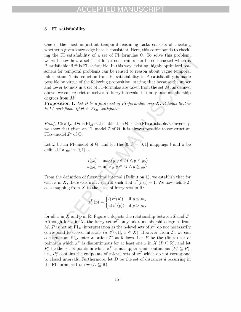
One of the most important temporal reasoning tasks consists of checkingwhether a given knowledge base is consistent. Here, this corresponds to check-ing the FI–satisfiability of a set of FI–formulas Θ. To solve this problem,we will show how a set Ψ of linear constraints can be constructed which isP–satisfiable iff Θ is FI–satisfiable. In this way, existing, highly optimized rea-soners for temporal problems can be reused to reason about vague temporalinformation. This reduction from FI–satisfiability to P–satisfiability is madepossible by virtue of the following proposition, stating that because the upperand lower bounds in a set of FI–formulas are taken from the set M , as definedabove, we can restrict ourselves to fuzzy intervals that only take membershipdegrees from M .Proposition 1. Let Θ be a finite set of FI–formulas over X. It holds that Θis FI–satisfiable iff Θ is FIM–satisfiable.

Proof. Clearly, if Θ is FIM–satisfiable then Θ is also FI–satisfiable. Conversely,we show that given an FI–model I of Θ, it is always possible to construct anFIM–model I∗ of Θ.

Let I be an FI–model of Θ, and let the [0, 1] − [0, 1] mappings l and u bedefined for y0 in [0, 1] as

l(y0) = max{y|y ∈ M ∧ y ≤ y0}u(y0) = min{y|y ∈ M ∧ y ≥ y0}

From the definition of fuzzy time interval (Definition 1), we establish that foreach x in X, there exists an mx in R such that xI(mx) = 1. We now define I ′

as a mapping from X to the class of fuzzy sets in R:

xI′(p) =

⎧⎨⎩l(xI(p)) if p ≤ mx

u(xI(p)) if p > mx

for all x in X and p in R. Figure 5 depicts the relationship between I and I ′.Although for x in X, the fuzzy set xI′

only takes membership degrees fromM , I ′ is not an FIM–interpretation as the α-level sets of xI′

do not necessarilycorrespond to closed intervals (α ∈]0, 1], x ∈ X). However, from I ′, we canconstruct an FIM–interpretation I∗ as follows. Let P be the (finite) set ofpoints in which xI′

is discontinuous for at least one x in X (P ⊆ R), and letP x

s be the set of points in which xI′is not upper semi–continuous (P x

s ⊆ P ),i.e., P x

s contains the endpoints of α-level sets of xI′which do not correspond

to closed intervals. Furthermore, let D be the set of distances d occurring inthe FI–formulas from Θ (D ⊆ R).

15

ACCEP

TED M

ANUSC

RIPT

ACCEPTED MANUSCRIPT

(a) xI (b) xI′

(c) xI∗

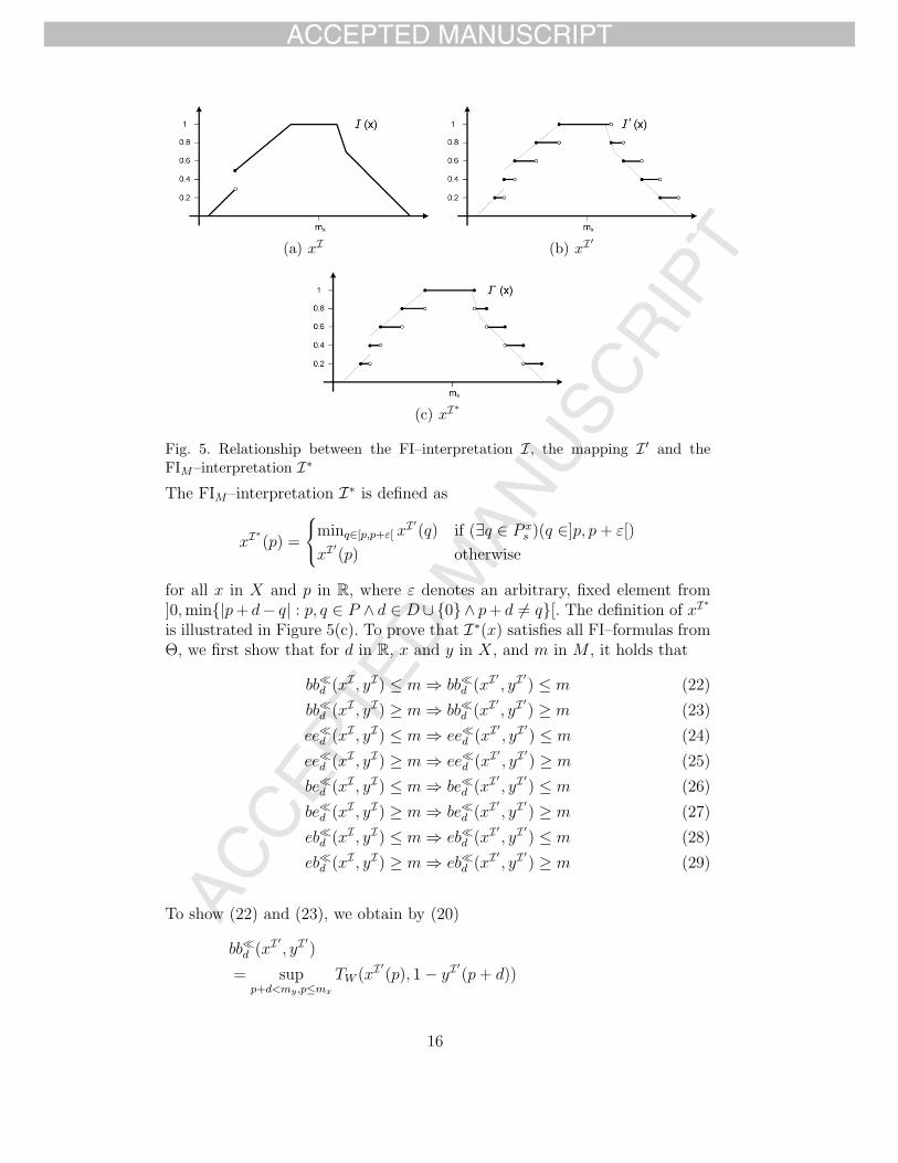
Fig. 5. Relationship between the FI–interpretation I, the mapping I ′ and theFIM–interpretation I∗

The FIM–interpretation I∗ is defined as

xI∗(p) =

⎧⎨⎩minq∈[p,p+ε[ x

I′(q) if (∃q ∈ P x

s )(q ∈]p, p + ε[)

xI′(p) otherwise

for all x in X and p in R, where ε denotes an arbitrary, fixed element from]0, min{|p + d− q| : p, q ∈ P ∧ d ∈ D ∪ {0} ∧ p + d �= q}[. The definition of xI∗

is illustrated in Figure 5(c). To prove that I∗(x) satisfies all FI–formulas fromΘ, we first show that for d in R, x and y in X, and m in M , it holds that

bb�d (xI , yI) ≤ m ⇒ bb�d (xI′, yI′

) ≤ m (22)

bb�d (xI , yI) ≥ m ⇒ bb�d (xI′, yI′

) ≥ m (23)

ee�d (xI , yI) ≤ m ⇒ ee�d (xI′, yI′

) ≤ m (24)

ee�d (xI , yI) ≥ m ⇒ ee�d (xI′, yI′

) ≥ m (25)

be�d (xI , yI) ≤ m ⇒ be�d (xI′, yI′

) ≤ m (26)

be�d (xI , yI) ≥ m ⇒ be�d (xI′, yI′

) ≥ m (27)

eb�d (xI , yI) ≤ m ⇒ eb�d (xI′, yI′

) ≤ m (28)

eb�d (xI , yI) ≥ m ⇒ eb�d (xI′, yI′

) ≥ m (29)

To show (22) and (23), we obtain by (20)

bb�d (xI′, yI′

)

= supp+d<my ,p≤mx

TW (xI′(p), 1 − yI′

(p + d))

16

ACCEP

TED M

ANUSC

RIPT

ACCEPTED MANUSCRIPT

= supp+d<my ,p≤mx

TW (xI(p) − (xI(p) − xI′(p)),

1 − yI(p + d) + (yI(p + d) − yI′(p + d)))

From the definition of I ′, it follows that (xI(p)− xI′(p)) ∈ [0, Δ[ and (yI(p +

d) − yI′(p + d)) ∈ [0, Δ[, for p + d < my and p ≤ mx. Hence, we have

≤ supp+d<my ,p≤mx

TW (xI(p), 1 − yI(p + d) + (yI(p + d) − yI′(p + d)))

≤ supp+d<my ,p≤mx

TW (xI(p), 1 − yI(p + d)) + (yI(p + d) − yI′(p + d))

< supp+d<my ,p≤mx

TW (xI(p), 1 − yI(p + d)) + Δ

= bb�d (xI , yI) + Δ

Similarly, we can show that

bb�d (xI′, yI′

) > bb�d (xI , yI) − Δ

Hence

bb�d (xI′, yI′

) − bb�d (xI , yI) ∈] − Δ, Δ[ (30)

Assume that bb�d (xI′, yI′

) > m would hold. Since both bb�d (xI′, yI′

) and mare contained in M , this implies that bb�d (xI′

, yI′) ≥ m + Δ. Using (30) we

establish that bb�d (xI , yI) > m also holds, proving (22) by contraposition. Inthe same way, we establish from bb�d (xI′

, yI′) < m that bb�d (xI′

, yI′) ≤ m−Δ

and thus bb�d (xI , yI) < m, proving (23). The implications (24)–(29) can beshown entirely analogously.

Next, we show that

bb�d (xI′, yI′

) = bb�d (xI∗, yI∗

) (31)

ee�d (xI′, yI′

) = ee�d (xI∗, yI∗

) (32)

be�d (xI′, yI′

) = be�d (xI∗, yI∗

) (33)

eb�d (xI′, yI′

) = eb�d (xI∗, yI∗

) (34)

First note that (31) immediately follows from the definition of I∗ by (20), asfor each p satisfying p ≤ mx and p+d < my, xI∗

(p) = xI′(p) and yI∗

(p+d) =yI′

(p + d). Turning now to (32), we find using (21) that

ee�d (xI′, yI′

) = supp−d>mx,p≥my

TW (yI′(p), 1 − xI′

(p − d)) (35)

ee�d (xI∗, yI∗

) = supp−d>mx,p≥my

TW (yI∗(p), 1 − xI∗

(p − d)) (36)

17

ACCEP

TED M

ANUSC

RIPT

ACCEPTED MANUSCRIPT

where mx and my are the smallest modal values of xI′and yI′

, or, equivalently,of xI∗

and yI∗. First, we show that for every p1 satisfying p1 − d > mx and

p1 ≥ my there exists a p2 satisfying p2 − d > mx and p2 ≥ my such that

TW (yI′(p1), 1 − xI′

(p1 − d)) = TW (yI∗(p2), 1 − xI∗

(p2 − d)) (37)

which already proves ee�d (xI′, yI′

) ≤ ee�d (xI∗, yI∗

). If yI′(p1) = yI∗

(p1) andxI′

(p1 − d) = xI∗(p1 − d) we can choose p2 = p1. Next, assume that yI′

(p1) >yI∗

(p1) and xI′(p1 − d) > xI∗

(p1 − d). This means that there is a q1 in P ys and

q2 in P xs such that q1 ∈]p1, p1 +ε[ and q2 ∈]p1−d, p1−d+ε[. The latter implies

that q2+d ∈]p1, p1+ε[ which, combined with the former, yields |q2+d−q1| < ε.By definition of ε, this is only possible if q2 = q1 − d, since for q2 + d �= q1, thedefinition of ε would imply ε < |q2 + d − q1|. We show that (37) is satisfiedfor p2 = q1 − ε. Note that mx, my ∈ P but mx /∈ P x

s and my /∈ P ys , hence

mx �= q2 and my �= q1, and even mx < q2 and my < q1. The definition of εimplies that ε < q1 + 0 − my and ε < q2 + 0 − mx. Since q2 = q1 − d andp2 = q1 − ε, this entails p2 ≥ my and p2 − d > mx. Since yI′

is constantover [q1 − ε, q1[, by definition of ε, it holds that yI∗

(q1 − ε) = yI′(q1 − ε), or

yI∗(p2) = yI′

(p2). As p1 ∈]q1 − ε, q1[, it holds that yI′is constant over [p2, p1],

hence yI′(p2) = yI′

(p1). In the same way, we establish xI∗(p2−d) = xI′

(p1−d).

If yI′(p1) > yI∗

(p1) and xI′(p1 − d) = xI∗

(p1 − d), there is a q1 in P ys such

that q1 ∈]p1, p1 + ε[. We show that (37) is satisfied for p2 = q1 − ε. As inthe previous case, the definition of ε implies that ε < q1 + 0 − my, hencep2 ≥ my. Again, we have that yI∗

(p2) = yI∗(q1 − ε) = yI′

(q1 − ε) = yI′(p2),

and yI′(p2) = yI′

(p1). Note that xI′is continuous in [q1−d−ε, q1−d[. Indeed,

if xI′were discontinuous in a point q2 in [q1 − d− ε, q1 − d[, it would hold that

0 < |q2 − q1 + d| ≤ ε, which is impossible by definition of ε. Since p1 − d > mx

and there are no discontinuities in [q1−d−ε, p1−d], we know that q1−d−ε >mx (recall that mx is the smallest modal value of xI′

). The continuity of xI′

in [q1−d− ε, q1−d[ furthermore implies that xI∗(q1−d− ε) = xI′

(q1−d− ε),and, since p1 − d < q1 − d, xI′

(q1 − d− ε) = xI′(p1 − d). From p2 = q1 − ε we

can conclude that xI∗(p2 − d) = xI′

(p1 − d)

The case where yI′(p1) = yI∗

(p1) and xI′(p1 − d) > xI∗

(p1 − d) is shownentirely analogously.

Conversely, we show that for every p2 satisfying p2 − d > mx and p2 ≥ my

there exists a p1 satisfying p1−d > mx and p1 ≥ my such that (37) is satisfied.If yI′

(p2) = yI∗(p2) and xI′

(p2 − d) = xI∗(p2 − d) we can choose p1 = p2. If

yI′(p2) > yI∗

(p2) and xI′(p2 − d) > xI∗

(p2 − d) there is a q1 in P ys and q2 in

P xs such that q1 ∈]p2, p2 + ε[ and q2 ∈]p2 − d, p2 − d + ε[. We show that (37) is

satisfied for p1 = q1. Again, this is only possible if q2 = q1 − d by definition ofε. First note that p1 = q1, q1 ∈]p2, p2 + ε[ and p2 ≥ my entail p1 ≥ my, whilep1 = q1, q1−d ∈]p2−d, p2+ε−d[ and p2−d > mx entail p1−d > mx. As q1 ∈ P y

s ,we know that yI′

is lower semi–continuous in q1. Since yI′is decreasing in q1,

18

ACCEP

TED M

ANUSC

RIPT

ACCEPTED MANUSCRIPT

this means that yI′is right–continuous in q1. Furthermore, by definition of ε

we know that yI′is continuous over [q1 − ε, q1[ and over ]q1, q1 + ε]. Together

with p2 ∈]q1 − ε, q1[, this yields yI∗(p2) = yI′

(q1) = yI′(p1). Similarly, we can

show that xI∗(p2 − d) = xI′

(q1 − d).

If yI′(p2) > yI∗

(p2) and xI′(p2 − d) = xI∗

(p2 − d) there is a q1 in P ys such

that q1 ∈]p2, p2 + ε[. We show that (37) is satisfied for p1 = q1. As before,we have that p1 ≥ my, p1 − d > mx, and yI∗

(p2) = yI′(q1). Note that xI′

iscontinuous in [q1 − d − ε, q1 − d[∪]q1 − d, q1 − d + ε]. Indeed, for every q2 in[q1 − d − ε, q1 − d + ε] \ {q1 − d}, it holds that 0 < |q2 − q1 + d| ≤ ε, whichimplies q2 /∈ P , using the definition of ε. If xI′

is also continuous in q1 − d,then obviously xI∗

(p2 − d) = xI′(q1 − d). If xI′

is upper semi–continuous inq1 − d then xI′

is also left–continuous (as xI′is decreasing in q1 − d), hence

xI′(q1 − d) = xI′

(p2 − d) = xI∗(p2 − d). Finally, we show that xI′

cannot belower semi–continuous in q1 − d. Indeed, this would imply that q1 − d ∈ P x

s

and thus xI′(p2 − d) > xI∗

(p2 − d), which contradicts the assumption thatxI′

(p2 − d) = xI∗(p2 − d).

The case where yI′(p1) = yI∗

(p1) and xI′(p1 − d) > xI∗

(p1 − d) is shown inthe same way.

Finally, (33) and (34) can be shown analogously.

From Lemma 1, we already know that upper and lower bounds of fuzzy tem-poral relations can be characterized by crisp temporal relations between theα–level sets of the fuzzy time intervals involved. As the next proposition shows,when these fuzzy time intervals only take membership degrees from M , only afinite number of α–level sets needs to be considered. The intuition behind thisproposition is that a fuzzy interval A taking only membership degrees fromM is completely characterized by the set of crisp intervals {AΔ, A2Δ, . . . , A1},which is in turn completely characterized by the set of instants (real numbers){A−

Δ, A−2Δ, . . . , A−

1 , A+1 , . . . , A+

2Δ, A+Δ}.

Proposition 2. Let A and B be fuzzy intervals that only take membershipdegrees from M , k ∈ M1 and l ∈ M0. It holds that:

bb�d (A, B) ≥ l ⇔ A−l < B−

Δ − d ∨ A−l+Δ < B−

2Δ − d

∨ · · · ∨ A−1 < B−

1−l+Δ − d (38)

bb�d (A, B) ≤ k ⇔ B−Δ ≤ A−

k+Δ + d ∧ B−2Δ ≤ A−

k+2Δ + d

∧ · · · ∧ B−1−k ≤ A−

1 + d (39)

ee�d (A, B) ≥ l ⇔ A+Δ < B+

l − d ∨ A+2Δ < B+

l+Δ − d

∨ · · · ∨ A+1−l+Δ < B+

1 − d (40)

ee�d (A, B) ≤ k ⇔ B+k+Δ ≤ A+

Δ + d ∧ B+k+2Δ ≤ A+

2Δ + d

∧ · · · ∧ B+1 ≤ A+

1−k + d (41)

be�d (A, B) ≥ l ⇔ A−l < B+

1 − d ∨ A−l+Δ < B+

1−Δ − d

19

ACCEP

TED M

ANUSC

RIPT

ACCEPTED MANUSCRIPT

∨ · · · ∨ A−1 < B+

l − d (42)

be�d (A, B) ≤ k ⇔ B+1 ≤ A−

k+Δ + d ∧ B+1−Δ ≤ A−

k+2Δ + d

∧ · · · ∧ B+k+Δ ≤ A−

1 + d (43)

eb�d (A, B) ≥ l ⇔ A+1 < B−

1−l+Δ − d ∧ A+1−Δ < B−

1−l+2Δ − d

∧ · · · ∧ A+1−l+Δ < B−

1 − d (44)

eb�d (A, B) ≤ k ⇔ B−1−k ≤ A+

1 + d ∨ B−1−k+Δ ≤ A+

1−Δ + d

∨ · · · ∨ B−1 ≤ A+

1−k + d (45)

Proof. As an example, we show (38). From Lemma 1 we already know that

bb�d (A, B) ≥ l ⇔ (∀ε ∈]0, l])(∃λ ∈]l − ε, 1])(bb�d (Aλ, Bλ+ε−l))

First note that if ε1 < ε2, B−λ+ε1−l ≤ B−

λ+ε2−l and therefore bb�d (Aλ, Bλ+ε1−l) ⇒bb�d (Aλ, Bλ+ε2−l). We thus obtain

bb�d (A, B) ≥ l ⇔ (∀ε ∈]0, Δ[)(∃λ ∈]l − ε, 1])(bb�d (Aλ, Bλ+ε−l))

Let ε ∈]0, Δ[ and let λ in ]l−ε, 1] be such that bb�d (Aλ, Bλ+ε−l). We first showthat there must exist some λ′ in {l, l + Δ, . . . , 1} such that bb�d (Aλ′ , Bλ′+ε−l).If λ ∈]l − ε, l[, then Aλ = Al as A only takes membership degrees fromM . Moreover, B−

λ+ε−l ≤ B−l+ε−l, hence from bb�d (Aλ, Bλ+ε−l) we establish

bb�d (Al, Bl+ε−l), i.e., we can choose λ′ = l. Similarly, if λ ∈]iΔ, (i + 1)Δ[(i ∈ N, l ≤ iΔ < (i + 1)Δ ≤ 1), we have that bb�d (Aλ, Bλ+ε−l) impliesbb�d (A(i+1)Δ, B(i+1)Δ+ε−l), and we can choose λ′ = (i + 1)Δ. This yields

bb�d (A, B) ≥ l ⇔ (∀ε ∈]0, Δ[)(∃λ ∈ {l, l + Δ, . . . , 1})(bb�d (Aλ, Bλ+ε−l))

Since now λ ∈ M and ε ∈]0, Δ[, we have that Bλ+ε−l = Bλ+Δ−l:

bb�d (A, B) ≥ l ⇔ (∀ε ∈]0, Δ[)(∃λ ∈ {l, l + Δ, . . . , 1})(bb�d (Aλ, Bλ+Δ−l))

⇔ (∃λ ∈ {l, l + Δ, . . . , 1})(bb�d (Aλ, Bλ+Δ−l))

proving (38).

Given a set of atomic FI–formulas Θ over a set of variables X, we constructa set of variables X ′ and a set of linear constraints Ψ over X ′ such that Θ isFI–satisfiable iff Ψ is P–satisfiable. From Proposition 1, we know that we canrestrict ourselves to fuzzy intervals that only take membership degrees fromM . Proposition 2 furthermore reveals that checking whether an FIM interpre-tatation satisfies an FI–formula can be done by evaluating a constant numberof linear inequalities. This suggests the following procedure for constructingX ′ and Ψ.

Let X ′ and Ψ initially be the empty set. For each variable x in X, we addthe new variables x−

Δ, x−2Δ, . . . , x−

1 , x+1 , . . . , x+

2Δ and x+Δ to X ′. Intuitively, these

20

ACCEP

TED M

ANUSC

RIPT

ACCEPTED MANUSCRIPT

new variables correspond to the beginning and ending points of α–level setsof the fuzzy interval corresponding with x. By adding the following linearconstraints to Ψ, for each m in M1 \ {0}, we ensure that in every P–model Iof Ψ, these new variables can indeed be interpreted as beginning and endingpoints of α-level sets of a fuzzy interval:

x−1 ≤ x+

1 (46)

x−m ≤ x−

m+Δ (47)

x+m+Δ ≤ x+

m (48)

In this way, every P–model I of Ψ corresponds to an FIM–interpretation I ′ ofΘ in which xI′

is the fuzzy interval taking only membership degrees from M ,defined through its α–level sets by (I ′(x))m = [I(x−

m), I(x+m)] for all m ∈ M0.

Finally, for each FI–formula in Θ, we add a particular set of linear constraintsto Ψ, based on the equivalences of Proposition 2. For example, if Θ containsthe FI–formula bb�d (x, y) ≤ k, we add the following set of linear constraints:

{y−Δ ≤ x−

k+Δ + d, y−2Δ ≤ x−

k+2Δ + d, . . . , y−1−k ≤ x−

1 + d} (49)

Similarly, if Θ contains the FI–formula bb�d (x, y) ≥ l, we add the followinglinear constraint:

x−l < y−

Δ − d ∨ x−l+Δ < y−

2Δ − d ∨ · · · ∨ x−1 < y−

1−l+Δ − d (50)

Clearly, Θ∪{r1∨r2} is FI–satisfiable iff either Θ∪{r1} is FI–satisfiable or Θ∪{r2} is FI–satisfiable. Therefore, we only needed to consider sets of atomic FI–formulas in the procedure described above. Nonetheless, this procedure is notinherently restricted to sets of atomic FI–formulas, as disjunctive FI–formulascorrespond to (sets of) linear constraints as well. However, the number of linearconstraints can be exponential in the number of disjuncts in the FI–formulas.

As expressed by the following proposition, it holds that the set of linear con-straints Ψ is P–satisfiable iff Θ is FI–satisfiable.Proposition 3. Let Θ be a finite set of atomic FI–formulas over X, andlet Ψ be the corresponding set of linear constraints over X ′, obtained by theprocedure outlined above. It holds that Θ is FI–satisfiable iff Ψ is P–satisfiable.

Proof. Assume that Θ is FI–satisfiable. Then there exists an FIM–model Iof Θ by Proposition 1. We define the P–interpretation I ′ for all variables x−

iΔ

and x+iΔ as (i ∈ N, Δ ≤ iΔ ≤ 1):

I ′(x−iΔ) = (xI)−iΔ (51)

I ′(x+iΔ) = (xI)+

iΔ (52)

21

ACCEP

TED M

ANUSC

RIPT

ACCEPTED MANUSCRIPT

Fig. 6. There exists an FIM–interpretation I for a set of FI-formulas Θ iff thereexists a P–interpretation I ′ for the corresponding set Ψ of linear constraints.

In other words, I ′(x−iΔ) and I ′(x+

iΔ) correspond to the beginning and endingof the iΔ–level set of the fuzzy time interval xI . Figure 6 illustrates the re-lationship between I and I ′. Clearly, I ′ satisfies (46)–(48). By Proposition 2,we also have that all (sets of) linear constraints like (49) and (50) are satisfied.Hence, I is a P–model of Ψ.

Conversely, assume that Ψ is P–satisfiable. Then there exists a P–model I ′ ofΨ. We define the FIM–interpretation I from I ′ as

xI(r) =

⎧⎨⎩max{λ|λ ∈ M ∧ r ∈ [I ′(x−

λ ), I ′(x+λ )]} if r ∈ [I ′(xΔ)−, I ′(xΔ)+]

0 otherwise

(53)

for each x in X and r in R. By construction of Ψ, we have that xI is a fuzzytime interval. Moreover, by Proposition 2, we establish that I satisfies everyFI-formula in Θ.

Interestingly, by reducing FI–satisfiability to P–satisfiability of a set of linearconstraints, we can impose additional constraints on the variables involved. Forexample, we can express that a given variable x corresponds to a crisp interval,rather than a fuzzy interval, by adding the linear constraints {x−

Δ = x−2Δ, x−

2Δ =x−

3Δ, . . . , x−1−Δ = x−

1 , x+1 = x+

1−Δ, . . . , x+2Δ = x+

Δ} to Ψ. By additionally addingx−

1 = x+1 , we can even ensure that x is always interpreted as an instant (time

point). Similarly, we can add x−1 < x+

1 to express that x should never beinterpreted as a time point. If we know that the beginning of x is inherentlygradual, we can even impose {x−

Δ < x−2Δ, x−

2Δ < x−3Δ, . . . , x−

1−Δ < x−1 }. Such

additional constraints can be very useful if it is a priori known which variablescorrespond to (possibly) vague events, crisp events, and instants. Moreover,adding such constraints does not change the computational complexity of thealgorithm.

Another important advantage of the reduction to P–satisfiability is that exist-

22

ACCEP

TED M

ANUSC

RIPT

ACCEPTED MANUSCRIPT

ing, optimized algorithms for reasoning about linear constraints can be used.Existing algorithms can not only be used for checking FI–satisfiability, butalso to find FI–models (or consistent scenarios) of FI–satisfiable sets of FI–formulas. This technique is illustrated in the following example.Example 1. Let Θ = {bb�10(a, b) ≥ 0.5, eb�5 (c, a) ≥ 0.5, eb�5 (b, c) ≥ 0.75}.We can choose Δ = 0.25, and thus M = {0, 0.25, 0.5, 0.75, 1}. The linearconstraints of the form (46)–(48) are given by

Ψ1 = {a−0.25 ≤ a−

0.5, a−0.5 ≤ a−

0.75, a−0.75 ≤ a−

1 , a−1 ≤ a+

1 ,

a+1 ≤ a+

0.75, a+0.75 ≤ a+

0.5, a+0.5 ≤ a+

0.25,

b−0.25 ≤ b−0.5, b−0.5 ≤ b−0.75, b

−0.75 ≤ b−1 , b−1 ≤ b+

1 ,

b+1 ≤ b+

0.75, b+0.75 ≤ b+

0.5, b+0.5 ≤ b+

0.25,

c−0.25 ≤ c−0.5, c−0.5 ≤ c−0.75, c

−0.75 ≤ c−1 , c−1 ≤ c+

1 ,

c+1 ≤ c+

0.75, c+0.75 ≤ c+

0.5, c+0.5 ≤ c+

0.25}

The additional linear constraints corresponding to the FI–formulas in Θ aregiven by

Ψ2 = {a−0.5 < b−0.25 − 10 ∨ a−

0.75 < b−0.5 − 10 ∨ a−1 < b−0.75 − 10,

c+1 < a−

0.75 − 5, c+0.75 < a−

1 − 5,

b+1 < c−0.5 − 5, b+

0.75 < c−0.75 − 5, b+0.5 < c−1 − 5}

The set Ψ of all linear constraints corresponding with Θ is then given byΨ1 ∪ Ψ2. It holds that Ψ can be satisfied by choosing the first disjunct a−

0.5 <b−0.25 − 10 in the disjunctive linear constraint a−

0.5 < b−0.25 − 10 ∨ a−0.75 < b−0.5 −

10 ∨ a−1 < b−0.75 − 10. In [20], an algorithm is presented to find a solution of

a set of atomic linear constraints, i.e., a P–interpretation I satisfying Ψ. Onepossible solution of Ψ is defined by

I(a−0.25) = I(a−

0.5) = I(c−0.25) = 0

I(a−0.75) = I(a−

1 ) = I(a+1 ) = I(a+

0.75) = I(a+0.5) = I(a+

0.25) = 22

I(b−0.25) = I(b−0.5) = I(b−0.75) = I(b−1 ) = 11

I(b+1 ) = I(b+

0.75) = I(b+0.5) = I(b+

0.25) = 11

I(c−0.5) = I(c−0.75) = I(c−1 ) = I(c+1 ) = I(c+

0.75) = I(c+0.5) = I(c+

0.25) = 16

As explained above, the P–model I of Ψ defines an FIM–model I ′ of Θ.

In applications, we usually need to find an FI–satisfiable set of FI–formulas,corresponding to some given (natural language) description, rather than check-ing the FI–satisfiablity of a given set of FI–formulas. Typically, in this context,the information provided may be inconsistent when interpreted as classical,crisp temporal relations. The goal is then to weaken information such as Ahappened before B to A happened before B at least to degree 0.8. The vari-ous lower and upper bounds introduced in this way (e.g., 0.8) should be the

23

ACCEP

TED M

ANUSC

RIPT

ACCEPTED MANUSCRIPT

strongest possible, w.r.t. a given precision Δ. The next example illustrates thisprocess.Example 2. Consider again the example about Picasso’s work from the intro-duction. To allow for a concise description, we use the following abbreviationsto refer to the relevant events and periods:

BFT Picasso creates Bread and Fruit Dish on a TableDMA Picasso creates the Demoiselles d’AvignonAC Picasso’s Analytical Cubism periodC Picasso’s Cubism period

The information that Bread and Fruit Dish on a Table marks the beginningof Picasso’s Analytical Cubism can be represented as

bb�(BFT,AC) ≥ λ1 (54)

bb�(AC, BFT ) ≥ λ2 (55)

ee�(BFT,AC) ≥ λ3 (56)

where initially λ1, λ2 and λ3 are assumed to be 1. Values lower than 1 areonly considered when inconsistencies arise. Similarly, the information that theDemoiselles d’Avignon marks the beginning of Picasso’s Cubist period can berepresented as

bb�(DMA, C) ≥ λ4 (57)

bb�(C, DMA) ≥ λ5 (58)

ee�(DMA, C) ≥ λ6 (59)

Next, the information that Analytical Cubism is the first stage of Picasso’sCubism can be represented by

bb�(AC, C) ≥ λ7 (60)

bb�(C, AC) ≥ λ8 (61)

ee�(AC, C) ≥ λ9 (62)

In addition to this qualitative description, we also have some quantitativeinformation. In particular, we know that Bread and Fruit Dish on a Table wascreated in 1909, the Demoiselles d’Avignon was created in 1907 and AnalyticalCubism lasted from somewhere in 1908 to somewhere in 1912. We can encodethis information using metric constraints by referring to an artificial time pointZ, for instance, corresponding to the beginning of the year 1900:

bb�8 (Z,AC) ≥ λ10 bb�−9(AC, Z) ≥ λ11 (63)

ee�12(Z,AC) ≥ λ12 ee�−13(AC, Z) ≥ λ13 (64)

bb�9 (Z,BFT ) ≥ λ14 ee�−10(BFT,Z) ≥ λ15 (65)

bb�7 (Z,DMA) ≥ λ16 ee�−8(DMA, Z) ≥ λ17 (66)

24

ACCEP

TED M

ANUSC

RIPT

ACCEPTED MANUSCRIPT

When checking the FI–satisfiability of this representation for various values ofthe lower bounds λi, we need to ensure that Z is a time point. As discussedabove, this can be done by adding the constraint Z−

Δ = Z−2Δ = · · · = Z−

1 =Z+

1 = · · · = Z+Δ to the corresponding set of linear constraints. From available

domain knowledge, we may moreover find out that creating a painting is acrisp event 6 , and therefore impose that DMA and BFT are crisp intervalsin a similar way.

For λ1 = λ2 = · · · = λ17 = 1, the description above is not FI–satisfiable.Hence, we need to weaken one or more of the lower bounds, i.e., we let someof the λi correspond to values from M lower than 1. Different sets of lowerbounds may be weakened to obtain an FI–satisfiable representation. Moreover,the actual strategy adopted to decide how to arrive at such a representationmay differ from application to application, as well as depend on additionalbackground information (e.g., degrees of confidence in each of the originalnatural language statements). In the example at hand, we may impose thatλ14 = λ15 = λ16 = λ17 = 1, as Z, BFT and DMA all refer to crisp events.Furthermore, we may initially require that λ1 = λ2 = · · · = λ13, as we lack anyfurther background knowledge for differentiating between the FI–formulas.Assuming Δ = 0.25, we first try λ1 = · · · = λ13 = 0.75, which is not FI–satisfiable, and next λ1 = · · · = λ13 = 0.5, which turns out to be FI–satisfiable.Although we have now arrived at an FI–satisfiable interpretation of the naturallanguage statements, it is not necessarily maximally FI–satisfiable, i.e., it maybe the case that not all of the λi’s (i ∈ {1, 2, . . . , 13}) need to be weakenedto 0.5. Therefore, we subsequently try to strengthen the λi’s again, one byone. For example, when λ2 = 0.75 or even λ2 = 1, the resulting representationremains FI–satisfiable. On the other hand, strengthening λ1 to 0.75 leads toa representation which is not FI–satisfiable anymore (even when λ2 = 0.5).Thus, after a linear number of FI–satisfiability checks, we obtain the followingmaximally FI–satisfiable representation:

λ14 = λ15 = λ16 = λ17 = 1

λ2 = λ3 = λ4 = λ6 = λ7 = λ8 = λ9 = λ10 = λ12 = λ13 = 1

λ1 = λ5 = λ11 = 0.5

A corresponding FI–interpretation is depicted in Figure 7, illustrating thatthe inconsistencies in the original natural language statements are causedby the vagueness of the Analytical Cubism and Cubism periods. In this FI–interpretation, both periods are assumed to have started in 1907 to degree 0.5,

6 Although the assumption made in this example is reasonable in most contexts,creating a painting could be seen as a vague event as well, assuming, for instance,that related studies and sketches made prior to the actual painting belong to thecreation to varying degrees.

25

ACCEP

TED M

ANUSC

RIPT

ACCEPTED MANUSCRIPT

Fig. 7. FI–interpretation of events corresponding to the creation of Bread and FruitDish on a Table (BFT ) and the Demoiselles d’Avignon (DMA), as well as Picasso’sAnalytical Cubism (AC) and Cubism (C) periods.

and to have started completely in 1909.

6 Computational complexity

Let A be a subset of FX , the set of all FI–formulas over a set of variables X.In the following discussion, we assume that X contains a sufficiently large, orinfinite number of different variables. We call FISAT(A) the problem of decid-ing whether a finite set of FI–formulas from A is FI–satisfiable. Deciding theP–satisfiability of an arbitrary set of linear constraints is NP–complete [44].To decide whether a set Θ of FI–formulas is FI–satisfiable, we can guess whichdisjuncts can be satisfied for all disjunctive FI–formulas, resulting in a set ofatomic FI–formulas Θ′. Checking if Θ′ is FI–satisfiable can be polyomiallyreduced to checking the P–satisfiability of a set of linear constraints, as ex-plained above. We thus find that FISAT(A) is in NP for every A ⊆ FX . As willbecome clear below, FISAT(FX) is also NP–hard and thereby NP–complete.However, checking the P–satisfiability of a set of linear constraints withoutdisjunctions is tractable [23,27]. From Proposition 2, it follows that a signif-icant subset of the FI–formulas do not lead to disjunctive linear constraints.We will refer to this subset as F t

X :

F tX =

⋃(x,y)∈X2

⋃d∈R

({bb�d (x, y) ≤ k|k ∈ M1} ∪ {ee�d (x, y) ≤ k|k ∈ M1}

∪ {be�d (x, y) ≤ k|k ∈ M1} ∪ {eb�d (x, y) ≥ l|l ∈ M0}∪ {bb�d (x, y) ≥ 1, ee�d (x, y) ≥ 1, be�d (x, y) ≥ 1, eb�d (x, y) ≤ 0}

)

Clearly FISAT(F tX) is tractable. Note, however, that the procedure described

above for deciding FISAT(F tX) is only weakly polynomial, as it depends on

the value of 1Δ

= ρ.

26

ACCEP

TED M

ANUSC

RIPT

ACCEPTED MANUSCRIPT

To support efficient reasoning, it is of interest to identify maximally tractablesubsets of FX , i.e., sets of FI–formulas A ⊆ FX such that FISAT(A) istractable and for any proper superset A′ of A, it holds that FISAT(A′) isNP–complete 7 . As we show in the following two propositions, when extend-ing F t

X with FI–formulas, it is not possible to keep tractability without puttingrestrictions on the variables.Proposition 4. Let k ∈ M1 \ {0} and d ∈ R. FISAT(A) is NP-complete if Acontains any of the following sets of FI-formulas:

F tX ∪ ⋃

(x,y)∈X2

{bb�d (x, y) ≥ k} (67)

F tX ∪ ⋃

(x,y)∈X2

{ee�d (x, y) ≥ k} (68)

F tX ∪ ⋃

(x,y)∈X2

{be�d (x, y) ≥ k} (69)

F tX ∪ ⋃

(x,y)∈X2

{eb�d (x, y) ≤ k} (70)

Proof. As an example, we show (67) for d = 0. The proof for (68)–(70) andd �= 0 is entirely analogous.

Since FISAT(FX) is in NP, we already have that FISAT(A) is in NP. Toestablish the NP-hardness of FISAT(A), we will show that 3SAT can be poly-nomially reduced to it. The proof is inspired by [37], where a similar reductionis made to prove NP-hardness for the satisfiability problem in a subfragmentof the Interval Algebra.

Let D = {C1, C2, . . . , Cn}, where Ci denotes a clause of the form li1 ∨ li2 ∨ li3,containing exactly three disjuncts. Each literal lij is either an atomic proposi-tion or the negation of an atomic proposition. 3SAT is the problem of decidingwhether D is satisfiable, i.e., deciding if there exists a truth assignment of theatomic propositions that makes all clauses from D true. To prove (67), wewill construct a set Θ of FI-formulas from A which is FI-satisfiable iff D issatisfiable, thereby reducing 3SAT to FISAT(A).

For each i in {1, . . . , n} and j in {1, 2, 3}, we add the following FI–formulasto Θ:

bb�(aij, bij) ≥ k (71)

bb�(cij, bij) ≤ k − Δ (72)

where aij, bij and cij are different variables from X.

7 Throughout the paper, we assume P �= NP.

27

ACCEP

TED M

ANUSC

RIPT

ACCEPTED MANUSCRIPT

Fig. 8. Linear constraints (73)–(74).

These FI-formulas correspond to the following linear constraints:

(aij)−k < (bij)

−Δ ∨ (aij)

−k+Δ < (bij)

−2Δ ∨ · · · ∨ (aij)

−1 < (bij)

−1−k+Δ (73)

{(bij)−Δ ≤ (cij)

−k , (bij)

−2Δ ≤ (cij)

−k+Δ, . . . , (bij)

−1−k+Δ ≤ (cij)

−1 } (74)

Linear constraints can be depicted as a graph in which nodes correspond tovariables, and edges labeled with < or ≤ are added between two nodes if <or ≤ is imposed on the corresponding variables. Figure 8 shows the graphcorresponding to (73)–(74). Linear constraints with disjunctions are displayedas dotted lines, as only one of several possible edges needs to be satisfied inthis case. Furthermore, we add the following FI–formulas to Θ:

bb�(ci1, di1) ≥ 1 bb�(ai2, di1) ≤ 1 − Δ

bb�(ci2, di2) ≥ 1 bb�(ai3, di2) ≤ 1 − Δ

bb�(ci3, di3) ≥ 1 bb�(ai1, di3) ≤ 1 − Δ

The corresponding linear constraints are given by

(ci1)−1 < (di1)

−Δ (di1)

−Δ ≤ (ai2)

−1 (75)

(ci2)−1 < (di2)

−Δ (di2)

−Δ ≤ (ai3)

−1 (76)

(ci3)−1 < (di3)

−Δ (di3)

−Δ ≤ (ai1)

−1 (77)

Figure 9 contains a graph corresponding to Figure 8 for ai1, bi1 and ci1, aswell as the graph for ai2, bi2 and ci2, and the graph for ai3, bi3 and ci3. Forclarity, the nodes for the bij–variables are omitted. Furthermore, these threesubgraphs are linked together by the constraints (75)–(77). If (ai1)

−1 < (ci1)

−1 ,

(ai2)−1 < (ci2)

−1 and (ai3)

−1 < (ci3)

−1 would hold, we obtain (ai1)

−1 < (ci1)

−1 <

(ai2)−1 < (ci2)

−1 < (ai3)

−1 < (ci3)

−1 < (ai1)

−1 , and thus (ai1)

−1 < (ai1)

−1 which

cannot be satisfied. Hence, every FI–model of Θ corresponds to a P–model inwhich at least one of (ai1)

−1 ≥ (ci1)

−1 , (ai2)

−1 ≥ (ci2)

−1 and (ai3)

−1 ≥ (ci3)

−1 holds.

A truth assignment that makes lij true if (aij)−1 ≥ (cij)

−1 will therefore make

all clauses in D true. To ensure that such a truth assignment indeed exists,what remains is to make sure that an atomic proposition lij and its negation,

28

ACCEP

TED M

ANUSC

RIPT

ACCEPTED MANUSCRIPT

Fig. 9. Linear constraints (75)–(77).

denoted below by lrs, are not made true simultaneously. If we want to definea correspondence between Θ and D, we therefore need to encode that one of(aij)

−1 < (cij)

−1 or (ars)

−1 < (crs)

−1 must hold. This can be accomplished by

adding the following FI–formulas to Θ:

bb�(eijrs, cij) ≤ Δ (78)

bb�(eijrs, fijrs) ≥ 1 (79)

bb�(ars, fijrs) ≤ k − Δ (80)

bb�(ersij, crs) ≤ Δ (81)

bb�(ersij, frsij) ≥ 1 (82)

29

ACCEP

TED M

ANUSC

RIPT

ACCEPTED MANUSCRIPT

bb�(aij, frsij) ≤ k − Δ (83)

which correspond to the following (sets of) linear constraints

{(cij)−Δ ≤ (eijrs)

−2Δ, (cij)

−2Δ ≤ (eijrs)

−3Δ, . . . , (cij)

−1−Δ ≤ (eijrs)

−1 } (84)

(eijrs)−1 < (fijrs)

−Δ (85)

{(fijrs)−Δ ≤ (ars)

−k , (fijrs)

−2Δ ≤ (ars)

−k+Δ, . . . , (fijrs)

−1−k+Δ ≤ (ars)

−1 } (86)

{(crs)−Δ ≤ (ersij)

−2Δ, (crs)

−2Δ ≤ (ersij)

−3Δ, . . . , (crs)

−1−Δ ≤ (ersij)

−1 } (87)

(ersij)−1 < (frsij)

−Δ (88)

{(frsij)−Δ ≤ (aij)

−k , (frsij)

−2Δ ≤ (aij)

−k+Δ, . . . , (frsij)

−1−k+Δ ≤ (aij)

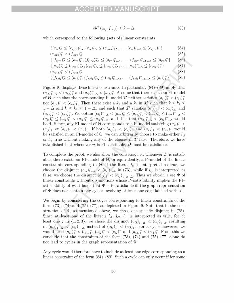
−1 } (89)

Figure 10 displays these linear constraints. In particular, (84)–(89) imply that(cij)

−1−Δ < (ars)

−k and (crs)

−1−Δ < (aij)

−k . Assume that there exists an FI-model

of Θ such that the corresponding P–model I ′ neither satisfies (aij)−1 < (cij)

−1

nor (ars)−1 < (crs)

−1 . Then there exist a k1 and a k2 in M such that k ≤ k1 ≤

1 − Δ and k ≤ k2 ≤ 1 − Δ, and such that I ′ satisfies (aij)−k1

< (cij)−k1

and(ars)

−k2

< (crs)−k2

. We obtain (cij)−1−Δ < (ars)

−k ≤ (ars)

−k2

< (crs)−k2

≤ (crs)−1−Δ <

(aij)−k ≤ (aij)

−k1

< (cij)−k1

≤ (cij)−1−Δ, and thus that (cij)

−1−Δ < (cij)

−1−Δ would

hold. Hence, any FI-model of Θ corresponds to a P–model satisfying (aij)−1 <

(cij)−1 or (ars)

−1 < (crs)

−1 . If both (aij)

−1 < (cij)

−1 and (ars)

−1 < (crs)

−1 would

be satisfied in an FI-model of Θ, we can arbitrarily choose to make either lijor lrs true without making any of the clauses in D false. Therefore, we haveestablished that whenever Θ is FI-satisfiable, D must be satisfiable.

To complete the proof, we also show the converse, i.e., whenever D is satisfi-able, there exists an FI–model of Θ, or equivalently, a P–model of the linearconstraints corresponding to Θ. If the literal lij is interpreted as true, wechoose the disjunct (aij)

−1−Δ < (bij)

−1−k in (73), while if lij is interpreted as

false, we choose the disjunct (aij)−1 < (bij)

−1−k+Δ. Thus we obtain a set Ψ of

linear constraints without disjunctions whose P–satisfiability implies the FI–satisfiability of Θ. It holds that Ψ is P–satisfiable iff the graph representationof Ψ does not contain any cycles involving at least one edge labeled with <.

We begin by considering the edges corresponding to linear constraints of theform (73), (74) and (75)–(77), as depicted in Figure 9. Note that in the con-struction of Ψ, as mentioned above, we chose one specific disjunct in (75).Since at least one of the literals li1, li2, li3 is interpreted as true, for atleast one j in {1, 2, 3}, we chose the disjunct (aij)

−1−Δ < (bij)

−1−k, resulting

in (aij)−1−Δ < (cij)

−1−Δ instead of (aij)

−1 < (cij)

−1 . For a cycle, however, we

would need (ai1)−1 < (ci1)

−1 , (ai2)

−1 < (ci2)

−1 and (ai3)

−1 < (ci3)

−1 . From this we

conclude that the constraints of the form (73), (74) and (75)–(77) alone donot lead to cycles in the graph representation of Ψ.

Any cycle would therefore have to include at least one edge corresponding to alinear constraint of the form (84)–(89). Such a cycle can only occur if for some

30

ACCEP

TED M

ANUSC

RIPT

ACCEPTED MANUSCRIPT

Fig. 10. Linear constraints (84)–(89).

i, j, r, s in {1, 2, . . . , n}, we have that (cij)−1−Δ < (ars)

−k , (ars)

−1−Δ < (crs)

−1−Δ,

(crs)−1−Δ < (aij)

−k and (aij)

−1−Δ < (cij)

−1−Δ. By construction, (cij)

−1−Δ < (ars)

−k

and (crs)−1−Δ < (aij)

−k are only implied by Ψ iff lij ≡ ¬lrs. However, if this is the

case, either lij or lrs is false, and (ars)−1−Δ < (crs)

−1−Δ and (aij)

−1−Δ < (cij)

−1−Δ

cannot both be contained in Ψ. Hence Ψ cannot contain any cycle, whichcompletes the proof.

Proposition 4 shows that, when no restrictions on the variables are imposed,F t

X cannot be extended with atomic FI–formulas without losing tractability.From the next proposition, it follows that this also holds for disjunctive FI-formulas.

31

ACCEP

TED M

ANUSC

RIPT

ACCEPTED MANUSCRIPT

Fig. 11. Linear constraints (93)–(95).

Proposition 5. Let rd and sd be bb�d , ee�d , be�d or eb�d (d ∈ R). FISAT(A)is NP-complete if A contains any of the following sets of FI-formulas:

F tX ∪ ⋃

(x,y,u,v)∈X4

{rd1(x, y) ≥ l1 ∨ sd2(u, v) ≥ l2} (90)

F tX ∪ ⋃

(x,y,u,v)∈X4

{rd1(x, y) ≥ l1 ∨ sd2(u, v) ≤ k2} (91)

F tX ∪ ⋃

(x,y,u,v)∈X4

{rd1(x, y) ≤ k1 ∨ sd2(u, v) ≤ k2} (92)

for any d1, d2 ∈ R, l1, l2 ∈ M0 and k1, k2 ∈ M1.

Proof. As an example, we show (90) for rd1 = sd2 = bb�0 . First note that if∪(x,y)∈X2{rd1(x, y) ≥ l1} �⊆ F t

X or ∪(u,v)∈X2{sd2(u, v) ≥ l2} �⊆ F tX , (90) follows

straightforwardly from Proposition 4. Therefore, we only need to consider thecase where l1 = l2 = 1. We will establish that FISAT(F t

X∪⋃

(x,y)∈X2{bb�(x, y) ≥1−Δ}), which is NP-complete by Proposition 4, can be polynomially reducedto FISAT(F t

X ∪ ⋃(x,y,u,v)∈X4{bb�(x, y) ≥ 1 ∨ bb�(u, v) ≥ 1}).

Let Θ1 be a set of FI–formulas from F tX ∪ ⋃

(x,y)∈X2{bb�(x, y) ≥ 1 − Δ}. Weconstruct a set Θ2 of FI-formulas from FISAT(F t

X ∪ ⋃(x,y,u,v)∈X4{bb�(x, y) ≥

1∨bb�(u, v) ≥ 1}) by replacing every FI-formula in Θ1 of the form bb�(x, y) ≥1 − Δ by the following FI-formulas

bb�(x, v) ≥ 1 ∨ bb�(u, y) ≥ 1

bb�(u, x) ≤ Δ

bb�(y, v) ≤ Δ

giving rise to the following linear constraints:

x−1 < v−

Δ ∨ u−1 < y−

Δ (93)

{x−Δ ≤ u−

2Δ, x−2Δ ≤ u−

3Δ, . . . , x−1−Δ ≤ u−

1 } (94)

{v−Δ ≤ y−

2Δ, v−2Δ ≤ y−

3Δ, . . . , v−1−Δ ≤ y−

1 } (95)

These linear constraints are depicted in Figure 11. On the other hand, thecorresponding FI–formula bb�(x, y) ≥ 1 − Δ from Θ1 gives rise to

x−1−Δ < y−

Δ ∨ x−1 < y−

2Δ

32

ACCEP

TED M

ANUSC

RIPT

ACCEPTED MANUSCRIPT

Let Ψ1 and Ψ2 be the sets of linear constraints corresponding to Θ1 and Θ2

respectively. By Proposition 3, it suffices to show that Ψ1 is P–satisfiable iffΨ2 is P–satisfiable. Clearly, if I is a P–model of Ψ2, I is also a P–model of Ψ1.Conversely, we show that if I is a P–model of Ψ1, there exists a P–model I ′ ofΨ2. For all variables a occurring in Ψ1, we define I ′(a) = I(a). Moreover, foradditional variables occurring in (93)–(95), I ′ is defined as follows. For eachk in {2Δ, 3Δ, . . . , 1}, we define

I ′(u−k ) = I(x−

k−Δ)

while for each k in {Δ, . . . , 1 − 2Δ, 1 − Δ}, we define

I ′(v−k ) = I(y−

k+Δ)

Finally, we define

I ′(u−Δ) = I ′(u−

2Δ)

I ′(v−1 ) = I ′(v−

1−Δ)

Note that I ′(x−1−Δ) < I ′(y−

Δ) ∨ I ′(x−1 ) < I ′(y−

2Δ) implies that I ′ satisfies (93),as I ′(x−

1−Δ) = I ′(u−1 ) and I ′(v−

Δ) = I ′(y−2Δ). Clearly, I ′ also satisfies (94) and

(95), hence I ′ is a P–model of Ψ2.

To find tractable sets of FI–formulas that are larger than F tX , we can impose

restrictions on the variables in the FI–formulas. For example, it can be shownthat bb�d (x, x) = ee�d (x, x) = eb�d (x, x) = 0 for any d ≥ 0 [41]. Hence, forexample, bb�d (x, x) ≤ k is satisfied by any FI–interpretation for every k ∈ M1,while no FI–interpretation can satisfy bb�d (x, x) ≥ l for l ∈ M0. Therefore, ifφ is an FI–formula from F t

X , FISAT(F tX ∪ {φ ∨ bb�d (x, x) ≤ k1 ∨ ee�d (x, x) ≤

k2 ∨ bb�d (z, z) ≥ l1}) is still tractable. In the same way, if k1 ≤ k2, a formulalike bb�d (x, y) ≥ k1 ∨ bb�d (x, y) ≤ k2 will be satisfied by any FI-interpretation.

These extensions of F tX are of limited practical value because of their rather

trivial character. More useful tractable extensions can be derived by consid-ering disjunctive FI–formulas that give rise to disjunctive linear constraintswhich are Horn. For example, let φ be an FI–formula from F t

X and let thecorresponding set of linear constraints be given by {ρ1, ρ2, . . . , ρs}. An FI–formula like φ ∨ bb�d (x, y) ≥ Δ ∨ bb�−d(y, x) ≥ Δ gives rise to the set of linearconstraints {α1, α2, . . . , αs}, where

αi = ρi ∨ x−Δ < y−

Δ − d ∨ x−2Δ < y−

2Δ − d ∨ · · · ∨ x−1 < y−

1 − d

∨ y−Δ − d < x−

Δ ∨ y−2Δ − d < x−

2Δ ∨ · · · ∨ y−1 − d < x−

1

= ρi ∨ x−Δ �= y−

Δ − d ∨ x−2Δ �= y−

2Δ − d ∨ · · · ∨ x−1 �= y−

1 − d

In other words, each αi is a Horn linear constraint (i ∈ {1, 2, . . . , s}), henceFISAT(F t

X ∪ {φ ∨ bb�d (x, y) ≥ Δ ∨ bb�d (y, x) ≥ Δ}) is tractable.

33

ACCEP

TED M

ANUSC

RIPT

ACCEPTED MANUSCRIPT

More generally, let the set GX of FI–formulas be defined as follows:

GX =⋃

(x,y)∈X2

⋃d∈R

{bb�d (x, y) ≥ Δ ∨ bb�−d(y, x) ≥ Δ,

ee�d (x, y) ≥ Δ ∨ ee�−d(y, x) ≥ Δ,

be�d (x, y) ≥ 1 ∨ be�−d(y, x) ≥ 1}

Furthermore, let HX be recursively defined as follows

(1) If φ ∈ F tX , then φ ∈ HX

(2) If φ1 ∈ HX and φ2 ∈ GX , then (φ1 ∨ φ2) ∈ HX

(3) HX contains no other elements

As any FI–formula in HX corresponds to a Horn linear constraint, or a set ofHorn linear constraints, we have that FISAT(HX) is tractable.

When Δ = 1 (i.e., M = {0, 1}), we know by Proposition 1 that a set of FI–formulas is FI–satisfiable iff there exists an interpretation that assigns a crispinterval to every variable. The set of FI–formulas HX is then exactly equal tothe set of all Horn linear constraints involving the endpoints of these crisp in-tervals. Hence, for Δ = 1, our (tractable) fuzzy temporal reasoning frameworkdegenerates to reasoning about (Horn) linear constraints. By decreasing thevalue of Δ to 1

2, 1

3, 1

4, 1

5, . . . , an increasingly higher expressiveness is achieved.

7 Entailment

Let Θ be a set of FI–formulas over X, and γ an FI–formula over X. We say thatΘ entails γ, written Θ |= γ, iff every FI–model of Θ is also an FI–model of {γ}.The notion of entailment is important for applications, because it allows todraw conclusions that are not explicitly contained in an initial set of assertions.Obviously, Θ |= γ if Θ and the negation of γ can never be satisfied at thesame time. For example, Θ |= bb�d (x, y) ≤ k iff Θ∪{bb�d (x, y) > k} is not FI–satisfiable. Unfortunately, our procedure for checking FI–satifiability cannotbe applied for strict inequalities like bb�d (x, y) > k, as Proposition 1 doesnot hold in this case. However, for every FIM–interpretation I, we have thatbb�d (xI , yI) > k iff bb�d (xI , yI) ≥ k + Δ. Inspired by this observation, we saythat Θ weakly entails γ (w.r.t. M), written Θ |=M γ iff every FIM–model of Θis also an FIM–model of {γ}. Checking weak entailment can straightforwardlybe reduced to checking FI–satisfiability.Proposition 6. Let Θ be a set of FI–formulas and let r(x, y) be one ofbb�d (x, y), ee�d (x, y), be�d (x, y) and eb�d (x, y) (d ∈ R, (x, y) ∈ X2). For kin M1 and l in M0 it holds that

34

ACCEP

TED M

ANUSC

RIPT

ACCEPTED MANUSCRIPT

(1) Θ |=M r(x, y) ≥ l iff Θ ∪ {r(x, y) ≤ l − Δ} is not FI–satisfiable.(2) Θ |=M r(x, y) ≤ k iff Θ ∪ {r(x, y) ≥ k + Δ} is not FI–satisfiable.

Proof. The proof follows trivially from the fact that for any FIM–interpretationI, r(xI , yI) < l implies r(xI , yI) ≤ l−Δ and r(xI , yI) > k implies r(xI , yI) ≥k + Δ.

As the name already suggests, weak entailment is a weaker notion than en-tailment, i.e., (Θ |= γ) ⇒ (Θ |=M γ). Nonetheless, weak entailment can stillbe used in applications to derive sound conclusions, by virtue of the followingproposition.Proposition 7. Let Θ be a set of FI–formulas and let r(x, y) be one ofbb�d (x, y), ee�d (x, y), be�d (x, y) and eb�d (x, y) (d ∈ R, (x, y) ∈ X2). For kin M1 \ {1 − Δ} and l in M0 \ {Δ} it holds that

(1) If Θ |=M r(x, y) ≥ l then Θ |= r(x, y) ≥ l − Δ(2) If Θ |=M r(x, y) ≤ k then Θ |= r(x, y) ≤ k + Δ

Proof. If Θ |=M r(x, y) ≥ l, then by Proposition 6, Θ∪{r(x, y) ≤ l−Δ} is notFI–satisfiable. Hence in every FI–interpretation of Θ, it holds that r(x, y) >l − Δ, and in particular, r(x, y) ≥ l − Δ. The second implication is shown inthe same way.

In the remainder of this section, we will investigate when weak entailmentcoincides with entailment, i.e., in which situations Proposition 6 also holds for(regular) entailment. Clearly Θ∪{φ1∨φ2∨· · ·∨φn} |= γ iff Θ∪{φ1} |= γ andΘ ∪ {φ2} |= γ and . . . and Θ ∪ {φn} |= γ. Therefore, we can restrict ourselvesto the case where Θ only contains atomic FI–formulas.

As we discussed in Section 5, for each set of FI–formulas Θ, we can find a setof linear constraints Ψ which is P–satisfiable iff Θ is FI–satisfiable. If Ψ doesnot contain any disjunctive linear constraints, we can represent Ψ as a graphG whose nodes correspond to variables like x−

l or x+l (l ∈ M0). If Ψ contains a

linear constraint x+d ≤ y, we add an edge from the node corresponding withx to the node corresponding with y which is labeled with (≤, d). Similarly, ifΨ contains a linear constraint x + d < y, we add an edge labeled with (<, d).The sum of two labels (≤, d1) and (≤, d2) is defined as (≤, d1 + d2), whilethe sum of (<, d1) and (≤, d2), (≤, d1) and (<, d2), or (<, d1) and (<, d2), isdefined as (<, d1 + d2). A cycle for which the edge labels sum up to (≤, d),with d > 0, or to (<, d′), with d′ ≥ 0, is called a forbidden cycle. It holds thatΨ is P–satisfiable iff there are no forbidden cycles in G [25]. If Ψ does containdisjunctive linear constraints, every choice of the disjuncts leads to a differentgraph representation, and Ψ is P–satisfiable as soon as one of these graphs isfree of forbidden cycles.

35

ACCEP

TED M

ANUSC

RIPT

ACCEPTED MANUSCRIPT

In the following, nodes corresponding to variables like x−l will be called be-

ginning nodes, while nodes corresponding to variables like x+l will be called

ending nodes. Furthermore, we will sometimes assume that Δ = 12p

for some

p ∈ N \ {0}. Nodes like x−l or x+

l will then be called white nodes if l ∈{2Δ, 4Δ, . . . , 1} and black nodes otherwise. Finally, for l ∈ M \ {0, Δ} andk ∈ M1, x−

l−Δ (resp. x+k+Δ) will be called the left neighbour of x−

l (resp. x+k ),

while x−k+Δ (resp. x+

l−Δ) will be called the right neighbour of x−k (resp. x+

l ).

Graphs representing linear constraints derived from a set of FI–formulas ex-hibit some interesting properties. In particular, the following two lemmas willbe useful in reducing entailment checking to FI–satisfiability checking, or,equivalently, weak entailment checking.Lemma 3. Let Δ = 1

2pfor some p ∈ N \ {0}, and let Θ be a (finite) set of

FI–formulas. Let Ψ be the corresponding set of linear constraints and let Gbe the graph representation corresponding to a particular choice of disjunctsfor the disjunctive constraints in Ψ. Furthermore, assume that there is a pathin G from v to u in which each edge either corresponds to a linear constraintof the form (46)–(48), or is the result of an FI–formula in Θ of the formbb�d (x, y) ≤ k, ee�d (x, y) ≤ k, be�d (x, y) ≤ k, or eb�d (x, y) ≥ l for some k in{0, 2Δ, 4Δ, . . . , 1 − 2Δ} and l in {2Δ, 4Δ, . . . , 1}). Assume, moreover, that:

(1) v is a black beginning node and u is a white beginning node, or(2) v is a white ending node and u is a black ending node, or(3) v is a white ending node and u is a white beginning node, or(4) v is a black beginning node and u is a black ending node.

It holds that there is a path in G from v to the left neighbour of u, as well asa path from the right neighbour of v to u. Moreover, for both paths, the edgelabels sum up to the same value as for the original path.

Proof. The proof is presented in Appendix A.3.

We define the right(resp. left) neighbour of an edge from v to u as the edgefrom the right (resp. left) neighbour of v to the right (resp. left) neighbour ofu.Lemma 4. Let Δ = 1

2pfor some p in N \ {0}, and let Θ and Ψ be defined

as before. Moreover, assume that all upper and lower bounds in Θ are takenfrom {0, 2Δ, 4Δ, . . . , 1}. Let I be a P–model of Ψ, and let G1 be the corre-sponding graph representation of Ψ without forbidden cycles. Let the graph G2

be constructed from G1 by replacing

(1) edges resulting from an FI–formula of the form bb�d (x, y) ≥ l by theirright neighbour if they start from a black beginning node;

(2) edges resulting from an FI–formula of the form ee�d (x, y) ≥ l by theirright neighbour if they start from a white ending node;

36

ACCEP

TED M

ANUSC

RIPT

ACCEPTED MANUSCRIPT

(3) edges resulting from an FI–formula of the form be�d (x, y) ≥ l or eb�d (x, y) ≤k by their right neighbour if they start from a black beginning node.

It holds that G2 does not contain any forbidden cycles.

Proof. The proof is presented in Appendix A.4

Using Lemma 3 and Lemma 4, we can show the following lemma about FI–satisfiability when all upper and lower bounds are of the form 2iΔ.Lemma 5. Let Δ = 1

2pfor some p in N \ {0}, let Θ be a set of atomic FI–

formulas in which all upper and lower bounds are taken from {0, 2Δ, 4Δ, . . . , 1}.For l in {0, 2Δ, 4Δ, . . . , 1 − 2Δ} and k in {2Δ, 4Δ, . . . , 1}, it holds that:

(1) Θ ∪ {bb�d (x, y) ≥ l + Δ} is FI–satisfiable iff Θ ∪ {bb�d (x, y) ≥ l + 2Δ} isFI–satisfiable;

(2) Θ ∪ {ee�d (x, y) ≥ l + Δ} is FI–satisfiable iff Θ ∪ {ee�d (x, y) ≥ l + 2Δ} isFI–satisfiable;

(3) Θ ∪ {be�d (x, y) ≥ l + Δ} is FI–satisfiable iff Θ ∪ {be�d (x, y) ≥ l + 2Δ} isFI–satisfiable;

(4) Θ ∪ {eb�d (x, y) ≤ k − Δ} is FI–satisfiable iff Θ ∪ {eb�d (x, y) ≤ k − 2Δ}is FI–satisfiable.

Proof. The proof is presented in Appendix A.5.

Finally, we can show the following characterization of entailment in terms ofFI–satisfiability for FI–formulas of the form bb�d (x, y) ≤ k, ee�d (x, y) ≤ k,be�d (x, y) ≤ k, and eb�d (x, y) ≥ l.Proposition 8. Let Θ be a set of atomic FI–formulas. It holds for k in M1

and l in M0 that

(1) Θ |= bb�d (x, y) ≤ k iff Θ ∪ {bb�d (x, y) ≥ k + Δ} is not FI–satisfiable;(2) Θ |= ee�d (x, y) ≤ k iff Θ ∪ {ee�d (x, y) ≥ k + Δ} is not FI–satisfiable;(3) Θ |= be�d (x, y) ≤ k iff Θ ∪ {be�d (x, y) ≥ k + Δ} is not FI–satisfiable;(4) Θ |= eb�d (x, y) ≥ l iff Θ ∪ {eb�d (x, y) ≤ l − Δ} is not FI–satisfiable.

Proof. As an example, we show that Θ |= bb�d (x, y) ≤ k iff Θ ∪ {bb�d (x, y) ≥k+Δ} is not FI–satisfiable. Clearly, if Θ∪{bb�d (x, y) ≥ k+Δ} is FI–satisfiable,then Θ �|= bb�d (x, y) ≤ k. Therefore, we only need to show that if there is an FI–model of Θ which does not satisfy bb�d (x, y) ≤ k, it holds that Θ∪{bb�d (x, y) ≥k + Δ} is FI–satisfiable.

Let I be an FI–model of Θ, and assume that bb�d (xI , yI) > k. There exists an nin N such that bb�d (xI , yI) ≥ k+ Δ

2n . Obviously, we have that Θ∪{bb�d (x, y) ≥k + Δ

2n} is FI–satisfiable. By letting Δ2n play the role of Δ, we obtain using

37

ACCEP

TED M

ANUSC

RIPT

ACCEPTED MANUSCRIPT

Lemma 5 that Θ ∪ {bb�d (x, y) ≥ k + Δ2n−1} is FI–satisfiable. Again applying

Lemma 5 reveals that also Θ ∪ {bb�d (x, y) ≥ k + Δ2n−2} is FI–satisfiable. By

repeating this argument n times, we find that Θ ∪ {bb�d (x, y) ≥ k + Δ} isFI–satisfiable.

To find a characterization of entailment for FI–formulas of the form bb�d (x, y) ≥l, ee�d (x, y) ≥ l, be�d (x, y) ≥ l, and eb�d (x, y) ≤ k, we restrict ourselves to thecase where Θ only contains FI–formulas from F t

X .Lemma 6. Let Δ = 1

2pfor some p ∈ N\{0}, let Θ be a set of FI–formulas from

F tX in which all upper and lower bounds are taken from {0, 2Δ, 4Δ, . . . , 1}. For

l in {0, 2Δ, 4Δ, . . . , 1 − 2Δ} and k in {2Δ, 4Δ, . . . , 1}, it holds that:

(1) Θ ∪ {be�d (x, y) ≤ k − Δ} is FI–satisfiable iff Θ ∪ {be�d (x, y) ≤ k − 2Δ}is FI–satisfiable;

(2) Θ ∪ {eb�d (x, y) ≥ l + Δ} is FI–satisfiable iff Θ ∪ {eb�d (x, y) ≥ l + 2Δ} isFI–satisfiable.

Moreover, for k in {4Δ, 6Δ, . . . , 1}, it holds that

(1) Θ∪{bb�d (x, y) ≤ k−Δ} is FI–satisfiable iff Θ∪{bb�d (x, y) ≤ k− 2Δ} isFI–satisfiable;

(2) Θ ∪ {ee�d (x, y) ≤ k − Δ} is FI–satisfiable iff Θ ∪ {ee�d (x, y) ≤ k − 2Δ}is FI–satisfiable.

Proof. The proof is presented in Appendix A.6.

Note that the FI–satisfiability of Θ ∪ {bb�d (x, y) ≤ Δ} does not necessarilyimply that Θ∪{bb�d (x, y) ≤ 0} is FI–satisfiable. For example, for d′+d > 0, itholds that {bb�d′ (y, x) ≤ 0, bb�d (x, y) ≤ Δ} is FI–satisfiable, while {bb�d′ (y, x) ≤0, bb�d (x, y) ≤ 0} is not. Similarly, we have that {ee�d′ (y, x) ≤ 0, ee�d (x, y) ≤Δ} is FI–satisfiable and {ee�d′ (y, x) ≤ 0, e�d (x, y) ≤ 0} is not.Proposition 9. Let Θ be a set of atomic FI–formulas from F t

X . For k in M1

and l in M0, it holds that

(1) Θ |= be�d (x, y) ≥ l iff Θ ∪ {be�d (x, y) ≤ l − Δ} is not FI–satisfiable;(2) Θ |= eb�d (x, y) ≤ k iff Θ ∪ {eb�d (x, y) ≥ k + Δ} is not FI–satisfiable.

Moreover, for l in M0 \ {Δ}, it holds that

(1) Θ |= bb�d (x, y) ≥ l iff Θ ∪ {bb�d (x, y) ≤ l − Δ} is not FI–satisfiable;(2) Θ |= ee�d (x, y) ≥ l iff Θ ∪ {ee�d (x, y) ≤ l − Δ} is not FI–satisfiable.

Proof. The proof is entirely analogous to the proof of Proposition 8, usingLemma 6 instead of Lemma 5.

38

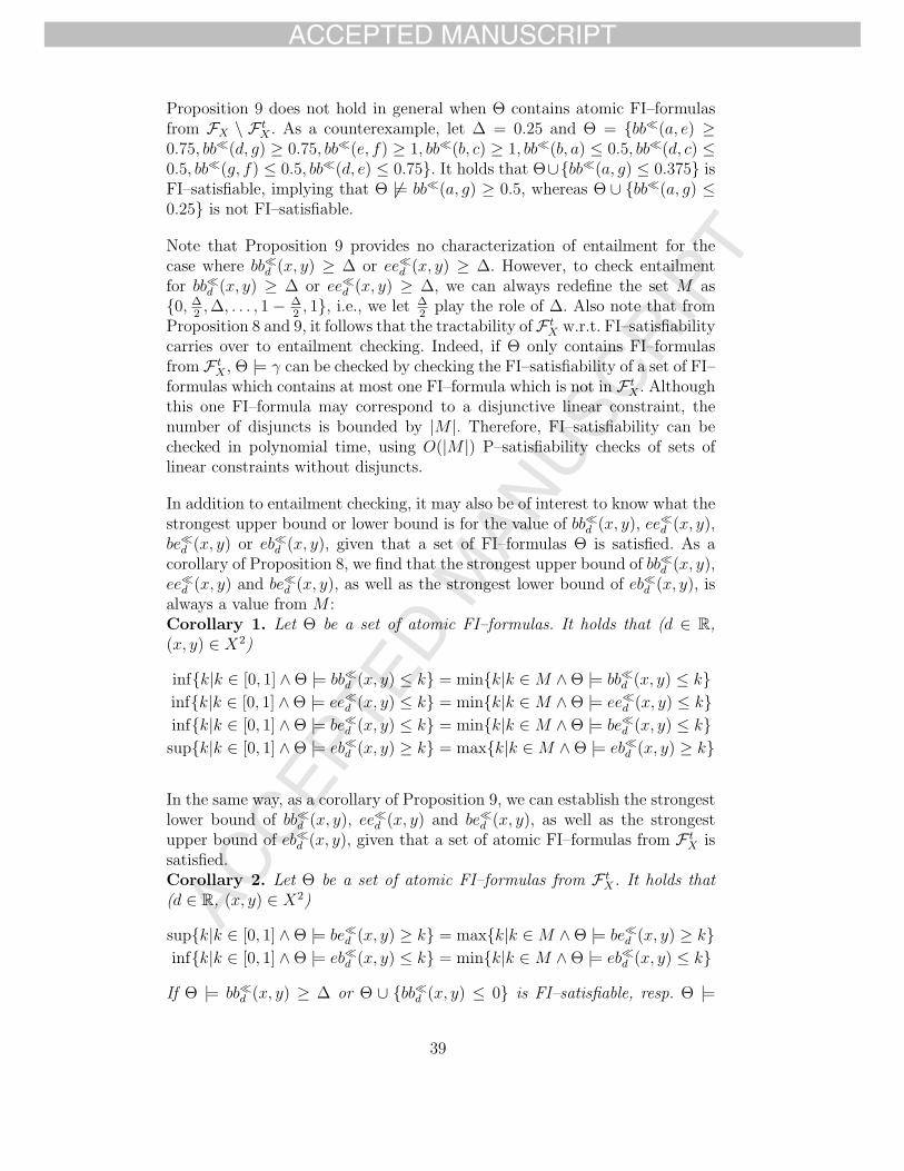
ACCEP

TED M

ANUSC

RIPT

ACCEPTED MANUSCRIPT

Proposition 9 does not hold in general when Θ contains atomic FI–formulasfrom FX \ F t

X . As a counterexample, let Δ = 0.25 and Θ = {bb�(a, e) ≥0.75, bb�(d, g) ≥ 0.75, bb�(e, f) ≥ 1, bb�(b, c) ≥ 1, bb�(b, a) ≤ 0.5, bb�(d, c) ≤0.5, bb�(g, f) ≤ 0.5, bb�(d, e) ≤ 0.75}. It holds that Θ∪{bb�(a, g) ≤ 0.375} isFI–satisfiable, implying that Θ �|= bb�(a, g) ≥ 0.5, whereas Θ ∪ {bb�(a, g) ≤0.25} is not FI–satisfiable.

Note that Proposition 9 provides no characterization of entailment for thecase where bb�d (x, y) ≥ Δ or ee�d (x, y) ≥ Δ. However, to check entailmentfor bb�d (x, y) ≥ Δ or ee�d (x, y) ≥ Δ, we can always redefine the set M as{0, Δ

2, Δ, . . . , 1 − Δ

2, 1}, i.e., we let Δ

2play the role of Δ. Also note that from

Proposition 8 and 9, it follows that the tractability of F tX w.r.t. FI–satisfiability

carries over to entailment checking. Indeed, if Θ only contains FI–formulasfrom F t

X , Θ |= γ can be checked by checking the FI–satisfiability of a set of FI–formulas which contains at most one FI–formula which is not in F t

X . Althoughthis one FI–formula may correspond to a disjunctive linear constraint, thenumber of disjuncts is bounded by |M |. Therefore, FI–satisfiability can bechecked in polynomial time, using O(|M |) P–satisfiability checks of sets oflinear constraints without disjuncts.

In addition to entailment checking, it may also be of interest to know what thestrongest upper bound or lower bound is for the value of bb�d (x, y), ee�d (x, y),be�d (x, y) or eb�d (x, y), given that a set of FI–formulas Θ is satisfied. As acorollary of Proposition 8, we find that the strongest upper bound of bb�d (x, y),ee�d (x, y) and be�d (x, y), as well as the strongest lower bound of eb�d (x, y), isalways a value from M :Corollary 1. Let Θ be a set of atomic FI–formulas. It holds that (d ∈ R,(x, y) ∈ X2)

inf{k|k ∈ [0, 1] ∧ Θ |= bb�d (x, y) ≤ k} = min{k|k ∈ M ∧ Θ |= bb�d (x, y) ≤ k}inf{k|k ∈ [0, 1] ∧ Θ |= ee�d (x, y) ≤ k} = min{k|k ∈ M ∧ Θ |= ee�d (x, y) ≤ k}inf{k|k ∈ [0, 1] ∧ Θ |= be�d (x, y) ≤ k} = min{k|k ∈ M ∧ Θ |= be�d (x, y) ≤ k}sup{k|k ∈ [0, 1] ∧ Θ |= eb�d (x, y) ≥ k} = max{k|k ∈ M ∧ Θ |= eb�d (x, y) ≥ k}

In the same way, as a corollary of Proposition 9, we can establish the strongestlower bound of bb�d (x, y), ee�d (x, y) and be�d (x, y), as well as the strongestupper bound of eb�d (x, y), given that a set of atomic FI–formulas from F t

X issatisfied.Corollary 2. Let Θ be a set of atomic FI–formulas from F t

X . It holds that(d ∈ R, (x, y) ∈ X2)

sup{k|k ∈ [0, 1] ∧ Θ |= be�d (x, y) ≥ k} = max{k|k ∈ M ∧ Θ |= be�d (x, y) ≥ k}inf{k|k ∈ [0, 1] ∧ Θ |= eb�d (x, y) ≤ k} = min{k|k ∈ M ∧ Θ |= eb�d (x, y) ≤ k}If Θ |= bb�d (x, y) ≥ Δ or Θ ∪ {bb�d (x, y) ≤ 0} is FI–satisfiable, resp. Θ |=

39

ACCEP

TED M

ANUSC

RIPT

ACCEPTED MANUSCRIPT

ee�d (x, y) ≥ Δ or Θ ∪ {ee�d (x, y) ≤ 0} is FI–satisfiable, it holds that

sup{k|k ∈ [0, 1] ∧ Θ |= bb�d (x, y) ≥ k} = max{k|k ∈ M ∧ Θ |= bb�d (x, y) ≥ k}sup{k|k ∈ [0, 1] ∧ Θ |= ee�d (x, y) ≥ k} = max{k|k ∈ M ∧ Θ |= ee�d (x, y) ≥ k}

Finally, if Θ |= bb�d (x, y) ≥ Δ while Θ∪{bb�d (x, y) ≤ 0} is not FI–satisfiable,resp. Θ |= ee�d (x, y) ≥ Δ while Θ ∪ {ee�d (x, y) ≤ 0} is not FI–satisfiable, itholds that in any FI–model I of Θ

bb�d (xI , yI) > 0

ee�d (xI , yI) > 0

while for any k > 0, there exists an FI–model I of Θ in which

bb�d (xI , yI) < k

ee�d (xI , yI) < k

In other words, in this last case, the strongest lower bound implied by Θ is astrict lower bound.

As becomes clear from Corollary 1 and 2, finding the strongest upper andlower bounds on bb�d (x, y), ee�d (x, y), be�d (x, y), or eb�d (x, y) implied by Θ canbe done by O(log(|M |)) FI–satisfiability checks, using binary search.

8 Concluding remarks

In this paper, we have shown how temporal reasoning about fuzzy time in-tervals can be reduced to reasoning about linear constraints. An importantadvantage of this approach is that we can draw upon well–established resultsfor solving disjunctive temporal reasoning problems, as well as reuse exist-ing, optimized tools for crisp temporal reasoning. The problem of satisfiabilitychecking was shown to be NP–complete. Hence, introducing vagueness in tem-poral reasoning does not increase the computational complexity. Moreover, animportant tractable subfragment HX was identified in this paper, which forΔ = 1 degenerates to the well–known framework of Horn linear constraints.In general, for Δ = 1 our framework degenerates to reasoning about crispintervals, i.e., if only 0 and 1 are used as upper and lower bounds, a set of FI–formulas can be satisfied by fuzzy time intervals iff it can be satisfied by crispintervals. For Δ = 0.5, the framework degenerates to reasoning about threevalued intervals. Such intervals can be represented as a pair of crisp intervals(a, a), where a contains the dates which fully belong to the vague time periodand a contains the dates which at least belong to the vague time period tosome extent (a ⊆ a). This essentially corresponds to a temporal counterpart

40

ACCEP

TED M

ANUSC

RIPT

ACCEPTED MANUSCRIPT

of the Egg-Yolk calculus [11] for spatial reasoning about vague regions. Fur-ther decreasing the value of Δ leads to an increasingly higher expressiveness,requiring, however, an increasing amount of computation time.

In contrast to crisp temporal reasoning frameworks, entailment checking in ourframework cannot straightforwardly be reduced to satisfiability checking. Tocope with this, we have introduced the notion of weak entailment, which canbe used to derive sound conclusions. Next, we have investigated in Proposition8 and Proposition 9 how entailment relates to weak entailment. Finally, wehave discussed how the strongest upper and lower bound on the possible valuesof a fuzzy temporal relation, applied to a particular pair of variables, can beobtained.

Our work is complementary to existing approaches for fuzzy temporal reason-ing, which have focused on modelling possibilistic uncertainty and preferences(e.g., [4]). An interesting direction for future work might be to combine ourframework with, for example, the IAfuz framework from [4] to allow temporalreasoning with uncertain information about vague time periods, or with fuzzytemporal constraint networks to allow imprecise metric constraints like “Ahappened about three weeks before B”. Further investigation is also needed tooptimize the reasoning procedures. Properties about the specific structure ofthe linear constraints that arise from a set of FI–formulas may be very usefulto prune the search space.

A Proofs

A.1 Proof of Lemma 1

First, we consider (12):

bb�d (A, B) ≥ l

⇔ supp∈R

TW (A(p), infq∈R

IW (B(q), L�d (p, q))) ≥ l

⇔ (∀ε > 0)(supp∈R

TW (A(p), infq∈R

IW (B(q), L�d (p, q))) > l − ε)

⇔ (∀ε > 0)(∃p ∈ R)(TW (A(p), infq∈R

IW (B(q), L�d (p, q))) > l − ε)

If A(p) = 0, it holds that T (A(p), infq∈R IT (B(q), L�d (p, q))) = 0. Therefore,

we can assume that A(p) > 0. Hence, there must exist a λ in ]0, 1] such thatλ = A(p) and thus p ∈ Aλ:

⇔ (∀ε > 0)(∃λ ∈]0, 1])(∃p ∈ Aλ)(TW (λ, infq∈R

IW (B(q), L�d (p, q))) > l − ε)

41

ACCEP

TED M

ANUSC

RIPT

ACCEPTED MANUSCRIPT

⇔ (∀ε > 0)(∃λ ∈]0, 1])(∃p ∈ Aλ)(λ + infq∈R

IW (B(q), L�d (p, q)) − 1 > l − ε)

⇔ (∀ε > 0)(∃λ ∈]0, 1])(∃p ∈ Aλ)(infq∈R

IW (B(q), L�d (p, q)) > l + 1 − λ − ε)

As any fuzzy time interval is upper semi–continuous, the mapping defined by1−B(q) for each q in R is lower semi–continous. Moreover, as L�

d (p, q) is lowersemi–continuous, the mapping defined by IW (B(q), L�

d (p, q)) for each q in R islower semi–continuous as well. Hence, the infimum infq∈R IW (B(q), L�

d (p, q))is attained for some q in R. We therefore find:

⇔ (∀ε > 0)(∃λ ∈]0, 1])(∃p ∈ Aλ)(∀q ∈ R)

(IW (B(q), L�d (p, q)) > l + 1 − λ − ε)

For λ ≤ l− ε, IW (B(q), L�d (p, q)) > l +1−λ− ε can never be satisfied, hence:

⇔ (∀ε > 0)(∃λ ∈]l − ε, 1])(∃p ∈ Aλ)(∀q ∈ R)

(IW (B(q), L�d (p, q)) > l + 1 − λ − ε)

If L�d (p, q) = 1, then IW (B(q), L�

d (p, q)) = 1, while IW (B(q), L�d (p, q)) =

1 − B(q) if L�d (p, q) = 0. We thereby obtain:

⇔ (∀ε > 0)(∃λ ∈]l − ε, 1])(∃p ∈ Aλ)(∀q ∈ R)

(L�d (p, q) = 1 ∨ 1 − B(q) > l + 1 − λ − ε)

⇔ (∀ε > 0)(∃λ ∈]l − ε, 1])(∃p ∈ Aλ)(∀q ∈ R)

(L�d (p, q) = 1 ∨ ¬(B(q) ≥ λ + ε − l))

If ε > l, then ¬(B(q) ≥ λ + ε− l)) can always be satisfied by choosing λ = 1.This yields:

⇔ (∀ε ∈]0, l])(∃λ ∈]l − ε, 1])(∃p ∈ Aλ)(∀q ∈ R)

(L�d (p, q) = 1 ∨ ¬(B(q) ≥ λ + ε − l))

⇔ (∀ε ∈]0, l])(∃λ ∈]l − ε, 1])(∃p ∈ Aλ)(∀q ∈ R)

(L�d (p, q) = 1 ∨ ¬(q ∈ Bλ+ε−l))

⇔ (∀ε ∈]0, l])(∃λ ∈]l − ε, 1])(∃p ∈ Aλ)(∀q ∈ R)(q ∈ Bλ+ε−l ⇒ L�d (p, q) = 1)

⇔ (∀ε ∈]0, l])(∃λ ∈]l − ε, 1])(bb�d (Aλ, Bλ+ε−l))

proving (12).

Turning now to (13), we find:

bb�d (A, B) ≤ k

⇔ supp∈R

TW (A(p), infq∈R

IW (B(q), L�d (p, q))) ≤ k

⇔ (∀p ∈ R)(TW (A(p), infq∈R

IW (B(q), L�d (p, q))) ≤ k) (A.1)

42

ACCEP

TED M

ANUSC

RIPT

ACCEPTED MANUSCRIPT

If A(p) = 0, then TW (A(p), infq∈R IW (B(q), L�d (p, q))) ≤ k is trivially satisfied.

Consequently, it is sufficient to show that for every p satisfying A(p) > 0, itholds that TW (A(p), infq∈R IW (B(q), L�

d (p, q))) ≤ k, or equivalently, to showthat for every λ ∈]0, 1] and every p in Aλ:

⇔ (∀λ ∈]0, 1])(∀p ∈ Aλ)(TW (A(p), infq∈R

IW (B(q), L�d (p, q))) ≤ k) (A.2)

which implies

(∀λ ∈]0, 1])(∀p ∈ Aλ)(TW (λ, infq∈R

IW (B(q), L�d (p, q))) ≤ k) (A.3)

since p ∈ Aλ means that A(p) ≥ λ. Conversely, we also have that (A.3) implies(A.2). Indeed, if (A.2) is violated, i.e., TW (A(p0), infq∈R IW (B(q), L�

d (p0, q))) >k for some λ0 ∈]0, 1] and some p0 ∈ Aλ0 , then (A.3) is violated for λ = A(p0)and p = p0. We conclude that (A.1) is equivalent to (A.3). We furthermorefind

(∀p ∈ R)(TW (A(p), infq∈R

IW (B(q), L�d (p, q))) ≤ k)

⇔ (∀λ ∈]0, 1])(∀p ∈ Aλ)(TW (λ, infq∈R

IW (B(q), L�d (p, q))) ≤ k)

⇔ (∀λ ∈]0, 1])(∀p ∈ Aλ)(λ + infq∈R

IW (B(q), L�d (p, q)) − 1 ≤ k)

⇔ (∀λ ∈]0, 1])(∀p ∈ Aλ)(infq∈R

IW (B(q), L�d (p, q)) ≤ 1 − λ + k)

If λ ≤ k, then IW (B(q), L�d (p, q)) ≤ 1 − λ + k is trivially satisfied. Therefore,

we have

⇔ (∀λ ∈]k, 1])(∀p ∈ Aλ)(infq∈R

IW (B(q), L�d (p, q)) ≤ 1 − λ + k)

⇔ (∀λ ∈]k, 1])(∀p ∈ Aλ)(∃q ∈ R)(IW (B(q), L�d (p, q)) ≤ 1 − λ + k)

⇔ (∀λ ∈]k, 1])(∀p ∈ Aλ)(∃q ∈ R)(L�d (p, q) = 0 ∧ B(q) ≥ λ − k)

⇔ (∀λ ∈]k, 1])(∀p ∈ Aλ)(∃q ∈ R)(L�d (p, q) = 0 ∧ q ∈ Bλ−k)

⇔ (∀λ ∈]k, 1])(∀p ∈ Aλ)(∃q ∈ Bλ−k)(L�d (p, q) = 0)

⇔ (∀λ ∈]k, 1])(∀p ∈ Aλ)(∃q ∈ Bλ−k)(¬(L�d (p, q) = 1))

⇔ (∀λ ∈]k, 1])(¬(∃p ∈ Aλ)(∀q ∈ Bλ−k)(L�d (p, q) = 1))

⇔ (∀λ ∈]k, 1])(¬bb�d (Aλ, Bλ−k))

⇔ (∀λ ∈]k, 1])(bb�d (Bλ−k, Aλ))

which proves (13). The characterizations (14)–(19) can be shown in the sameway as (12) or (13).

43

ACCEP

TED M

ANUSC

RIPT

ACCEPTED MANUSCRIPT

A.2 Proof of Lemma 2

By definition of bb�d , we obtain

bb�d (A, B)

= supp∈R

TW (A(p), infq∈R

IW (B(q), L�d (p, q)))

= max( supp≥mb−d

TW (A(p), infq∈R

IW (B(q), L�d (p, q))),

supp<mb−d

TW (A(p), infq∈R

IW (B(q), L�d (p, q))))

From the convexity of B, we establish that B is increasing for values smallerthan mb and decreasing for values greater than mb. Hence, we obtain

infq∈R

IW (B(q), L�d (p, q)) =

⎧⎨⎩IW (B(p + d), L�

d (p, p + d)) if p < mb − d

IW (B(mb), L�d (p, mb)) if p ≥ mb − d

We thus find

max( supp≥mb−d

TW (A(p), infq∈R

IW (B(q), L�d (p, q))),

supp<mb−d

TW (A(p), infq∈R

IW (B(q), L�d (p, q))))

= max( supp≥mb−d

TW (A(p), IW (B(mb), L�d (p, mb))),

supp<mb−d

TW (A(p), IW (B(p + d), L�d (p, p + d))))

= max( supp≥mb−d

TW (A(p), IW (1, 0)), supp<mb−d

TW (A(p), IW (B(p + d), 0)))

= max( supp≥mb−d

TW (A(p), 0), supp<mb−d

TW (A(p), 1 − B(p + d)))

= supp<mb−d

TW (A(p), 1 − B(p + d))

Due to its convexity, A is increasing for values smaller than ma and decreasingfor values greater than ma. Hence if p < mb − d and p > ma, it holds thatTW (A(p), 1−B(p+d))) ≤ TW (A(ma), 1−B(ma +d)). Therefore, we have that

supp<mb−d

TW (A(p), 1 − B(p + d)) = supp<mb−d,p≤ma

TW (A(p), 1 − B(p + d))

proving (20). Eq. (21) is shown entirely analogously.

44

ACCEP

TED M

ANUSC

RIPT

ACCEPTED MANUSCRIPT

A.3 Proof of Lemma 3

As an example, we show that there is a path from v to the left neighbourof u when v is a black beginning node and u is a white beginning node. Letv0 = v, v1, v2, . . . , vn = u be a path in G from v to u. If an edge from vj to vj+1

in G corresponds to a linear constraint that is the result of an FI–formula ofthe form bb�d (x, y) ≤ k, with k ∈ {0, 2Δ, 4Δ, . . . , 1−2Δ}, then vj and vj+1 areeither both white beginning nodes, or both black beginning nodes. If this edgeis the result of an FI–formula of the form ee�d (x, y) ≤ k, vj and vj+1 are bothwhite ending nodes or both black ending nodes. Finally, if the edge from vj tovj+1 is the result of an FI–formula of the form be�d (x, y) ≤ k, or an FI–formulaof the form eb�d (x, y) ≥ l, with l ∈ {2Δ, 4Δ, . . . , 1}, either vj is a white endingnode and vj+1 a black beginning node, or vj is a black ending node and vj+1

a white beginning node. The only remaining possibility is that the edge fromvj to vj+1 corresponds to a linear constraint of the form (46)–(48).

First assume that none of the edges on the path from v to u corresponds toa linear constraint of the form (46)–(48). Then all of the nodes v1, . . . , vn−1

need to be beginning nodes, as none of the remaining types of edges startsat a beginning node and ends at an ending node. This means that all edges(v0, v1), (v1, v2), . . . , (vn−1, vn) would correspond to a linear constraint that isthe result of an FI–formula of the form bb�d (x, y) ≤ k. Thus, from the factthat v is a black node, we establish that v1, v2, . . . , vn are all black nodes. This,however, is not possible since u = vn is a white beginning node.

Hence, at least one of the edges corresponds to a linear constraint of the form(46)–(48). Let (vs, vs+1) be the last of these edges. If (vs, vs+1) corresponds toan edge of the form (46), vs+1 is a white ending node. Then all edges betweenvs+1 and vn correspond to FI–formulas of the form ee�d (x, y) ≤ k, be�d (x, y) ≤k, or eb�d (x, y) ≥ l. This would imply that the nodes vs+2, vs+3, . . . , vn are allwhite ending nodes or black beginning nodes. This, however, is not possiblesince u = vn is a white beginning node. Therefore, (vs, vs+1) has to correspondto either (47) or (48). In both cases, vs+1 is the right neighbour of vs, and thepath v0, v1, . . . , vs, v

′s+2, v

′s+3, . . . , v

′n, where v′

i denotes the left neighbour of vi,is a path from v to the left neighbour v′

n of u. Moreover, the edge labels ofv′

s+2, v′s+3, . . . , v

′n are the same as those of vs+2, vs+3, . . . , vn (i.e., (≤, 0)), and

the edge label of (vs, vs+1) is (≤, 0), which adds nothing to the sum of the edgelabels on the original path.

45

ACCEP

TED M

ANUSC

RIPT

ACCEPTED MANUSCRIPT

Fig. A.1. The forbidden cycle in G2 is independent from the fact that the edge(v′r, v′r+1) in G1 was replaced by (vr, vr+1).

A.4 Proof of Lemma 4

Assume that G2 contains a forbidden cycle v1, v2, . . . , vn, v1, and let (vr, vr+1)be an edge in G2 that does not occur in G1. Then (vr, vr+1) is the rightneighbour of the edge (v′

r, v′r+1) from G1.

Moreover, first assume that vr is a white beginning node and vr+1 is a blackbeginning node. Suppose that the edge from vr to vr+1 is the only edgein the cycle that corresponds to an FI–formula of the form bb�d (x, y) ≥ l,ee�d (x, y) ≥ l, be�d (x, y) ≥ l or eb�d (x, y) ≤ k. This means that the pathvr+1, vr+2, . . . , vn, v1, . . . , vr in G2 also exists in G1. Indeed, none of the con-straints on the edges of this path fulfills the conditions for replacement in theconstruction process of G2 from G1. Furthermore, all of the constraints on theedges of this path fulfill the conditions of Lemma 3. Hence, we establish thatin G1 there is a path from vr+1 to v′

r whose edge labels sum up to the samevalue as the edge labels of the path vr+1, vr+2, . . . , vr−1, vr. This would meanthat G1 contains the forbidden cycle consisting of the path from vr+1 to v′

r,the edge from v′

r to v′r+1 and the edge from v′

r+1 to vr+1. Note that the latteredge exists since v′

r+1 is the left neighbour of vr+1.

Therefore, at least two edges in the forbidden cycle have to correspond toan FI–formula of the form bb�d (x, y) ≥ l, ee�d (x, y) ≥ l, be�d (x, y) ≥ l oreb�d (x, y) ≤ k. Let the edge from vs to vs+1 be the first such edge in the for-bidden cyle after vr+1, and let the edge from vt to vt+1 be the last such edge inthe forbidden cycle before vr (where r + 1 = s or t + 1 = r are also allowed).Figure A.1 depicts the forbidden cycle. It holds that vs is either a white be-ginning node or a black ending node, because of the way we transformed G1

to G2. In both cases, we can establish by Lemma 3 that there is a path fromvr+1 to the left neighbour v′

s of vs whose edge labels sum up to the same value

46

ACCEP

TED M

ANUSC

RIPT

ACCEPTED MANUSCRIPT

as those of the path from vr+1 to vs. In the same way, we have by constructionof G2 that vt+1 is either a black beginning node or a white ending node. FromLemma 3, we obtain that there is a path from vt+1 to v′

r, whose edge labelssum up to the same value as those of the path from vt+1 to vr.

Thus we have established that the forbidden cycle in G2 is independent fromthe fact that the edge (v′

r, v′r+1) in G1 was replaced by (vr, vr+1). In a similar

way, we can show this result when vr is a black ending node and vr+1 is awhite ending node, or when vr is a white beginning node and vr+1 is a whiteending node. We can repeat this argument for every edge that was changed inthe transformation from G1 to G2. Hence, if G2 contained a forbidden cycle,then G1 would contain a forbidden cycle as well.

A.5 Proof of Lemma 5

As an example, we show that Θ ∪ {bb�d (x, y) ≥ l + Δ} is FI–satisfiable iffΘ ∪ {bb�d (x, y) ≥ l + 2Δ} is FI–satisfiable. If Θ is not FI–satisfiable, or xor y does not occur in the FI–formulas in Θ, the proof is trivial. Therefore,assume that Θ is FI–satisfiable and contains both FI–formulas involving xand FI–formulas involving y. If Θ ∪ {bb�d (x, y) ≥ l + Δ} is not FI–satisfiable,then clearly Θ ∪ {bb�d (x, y) ≥ l + 2Δ} is not FI–satisfiable either. Hence, weonly need to show that if Θ ∪ {bb�d (x, y) ≥ l + 2Δ} is not FI–satisfiable,Θ ∪ {bb�d (x, y) ≥ l + Δ} cannot be FI–satisfiable.

Let Ψ be the set of linear constraints corresponding to the FI–formulas inΘ, and let I be a P–model of Ψ. The linear constraint corresponding tobb�d (x, y) ≥ l + Δ is given by:

x−l+Δ < y−

Δ − d ∨ x−l+2Δ < y−

2Δ − d ∨ · · · ∨ x−1 < y−

1−l − d (A.4)

while the linear constraint corresponding to bb�d (x, y) ≥ l + 2Δ is given by

x−l+2Δ < y−

Δ − d ∨ x−l+3Δ < y−

2Δ − d ∨ · · · ∨ x−1 < y−

1−l−Δ − d (A.5)

If Θ∪{bb�d (x, y) ≥ l+2Δ} is not FI–satisfiable, a forbidden cycle emerges whenadding an edge corresponding to any of the disjuncts of (A.5) to the graphrepresentation of Θ which corresponds with I. This means that any P–model ofΘ will correspond to a choice of disjuncts that leads to a graph representationG of Θ in which there is a path from y−

Δ to x−l+2Δ, a path from y−

2Δ to x−l+3Δ,

etc. Moreover, the edge labels of the path from y−(i+1)Δ to x−

l+(2+i)Δ sum up to

a value (di,≤) or (di, <) such that di + d ≥ 0 (i ∈ {0, 1, 2, . . . , 1−lΔ

− 2}).

We now transform the graph G to a graph G′ by applying the transformationfrom Lemma 4. The changing of edges in this transformation corresponds to

47

ACCEP

TED M

ANUSC

RIPT

ACCEPTED MANUSCRIPT

choosing different disjuncts for the disjunctive linear constraints in Ψ. As thistransformation cannot introduce forbidden cycles, the graph G′ correspondsto a P–model of Ψ. Therefore G′ contains a path from y−

(i+1)Δ to x−l+(2+i)Δ for

every i in {0, 1, 2, . . . , 1−lΔ

− 2}. Let y−Δ = v0, v1, v2, . . . , vn = x−

l+2Δ be a pathfrom y−

Δ to x−l+2Δ.

If this path contains no edges that correspond to an FI–formula of the formbb�d′ (x

′, y′) ≥ l′, ee�d′ (x′, y′) ≥ l′, be�d′ (x

′, y′) ≥ l′ or eb�d′ (x′, y′) ≤ k′, we can

apply Lemma 3 to establish that there is a path in G′ from y−Δ to x−

l+Δ, theleft neighbour of vn, and a path from y−

2Δ, the right neighbour of y−Δ, to x−

l+2Δ.As none of the edges in these paths are changed in the transformation fromG to G′, these paths also occur in G.

Next, assume that the path from v0 to vn contains at least one edge whichcorresponds to an FI–formula of the form bb�d′ (x

′, y′) ≥ l′, ee�d′ (x′, y′) ≥ l′,

be�d′ (x′, y′) ≥ l′ or eb�d′ (x

′, y′) ≤ k′. Let (vs, vs+1) and (vr, vr+1) be the first andlast of these edges respectively. Then vs is either a white beginning node ora black ending node, because of the nature of the transformation from G toG′. The path between v0 and vs therefore satisfies the conditions of Lemma3. Thus we find that G′ contains a path from y−

2Δ, the right neighbour of y−Δ,

to x−l+2Δ. Similarly, vr+1 is either a black beginning node, or a white ending

node. By Lemma 3 we find that G′ contains a path from y−Δ to x−

l+Δ, the leftneighbour of vn.

In the same way, we find from the fact that G′ contains a path from y−3Δ to

x−l+4Δ that G′ also contains a path from y−

3Δ to x−l+3Δ and from y4Δ to x−

l+4Δ, etc.Adding an edge to G′ corresponding to any of the disjuncts in (A.4) thereforeleads to a forbidden cycle in G′. Using Lemma 4, we can conclude from thisthat adding an edge to G corresponding to any of the disjuncts in (A.4) wouldlead to a forbidden cycle as well. Hence, in any P–model of Θ, it holds thatneither x−

l+Δ < y−Δ − d, x−

l+2Δ < y−2Δ − d, . . . , or x−

1 < y−1−l − d can be satisfied,

or, in other words, that Θ ∪ {bb�d (x, y) ≥ l + Δ} is not FI–satisfiable.

A.6 Proof of Lemma 6

As an example, we show that for k ∈ {4Δ, 6Δ, . . . , 1}, Θ∪{bb�d (x, y) ≤ k−Δ}is FI–satisfiable iff Θ ∪ {bb�d (x, y) ≤ k − 2Δ} is FI–satisfiable. Clearly, ifΘ∪{bb�d (x, y) ≤ k− 2Δ} is FI–satisfiable, then also Θ∪{bb�d (x, y) ≤ k−Δ}is FI–satisfiable. Conversely, we show that if Θ ∪ {bb�d (x, y) ≤ k − 2Δ} is notFI–satisfiable, then also Θ ∪ {bb�d (x, y) ≥ k − Δ} is not FI–satisfiable.

Let Ψ be the set of linear constraints corresponding to Θ. The linear con-

48

ACCEP

TED M

ANUSC

RIPT

ACCEPTED MANUSCRIPT

straints corresponding to bb�d (x, y) ≤ k − 2Δ are given by:

{y−Δ ≤ x−

k−Δ + d, y−2Δ ≤ x−

k + d, . . . , y−1−k+2Δ ≤ x−

1 + d} (A.6)

while the linear constraints corresponding to bb�d (x, y) ≤ k − Δ are given by

{y−Δ ≤ x−

k + d, y−2Δ ≤ x−

k+Δ + d, . . . , y−1−k+Δ ≤ x−

1 + d} (A.7)

Assume that Θ∪ {bb�d (x, y) ≤ k − 2Δ} is not FI–satisfiable. This means thatthe graph G corresponding to the linear constraints in Ψ contains a path fromx−

k−Δ to y−Δ, or a path from x−

k to y−2Δ, or . . . , or a path from x−

1 to y−1−k+2Δ.

Moreover, the edge labels in this path sum up to (<, d′) where d′ + d ≥ 0, or(≤, d′′) where where d′′ + d > 0, i.e., adding the edges corresponding to (A.6)would introduce a forbidden cycle in the graph. Note that there is only onegraph G corresponding to Ψ, as Ψ contains no disjunctive linear constraints.

Let v1, v2, . . . , vn be a path from x−k+(i−1)Δ to y−

(1+i)Δ, for some i in {0, 1, . . . , 1+1−kΔ

}, where v1 and vn are both white beginning nodes or both black beginningnodes. First assume that this path contains no edges corresponding to anFI–formula of the form bb�d′ (x

′, y′) ≥ 1, ee�d′ (x′, y′) ≥ 1, be�d′ (x

′, y′) ≥ 1 oreb�d′ (x

′, y′) ≤ 0. Note that edges corresponding to FI–formulas of the formee�d (x, y) ≤ k, be�d (x, y) ≤ k, and eb�d (x, y) ≥ l always start at an endingnode. Hence, either the path from v1 to vn contains no edges of the formee�d (x, y) ≤ k, be�d (x, y) ≤ k, and eb�d (x, y) ≥ l, or this path contains at leastone edge corresponding to (46). In the former case, however, it is not possibleto obtain a path from a node a−

k1to a node b−k2

if k1 > k2. Hence, since k > 2Δ,the path from v1 to vn needs to contain at least one edge of the form (46).Assume that v1 and vn are white beginning nodes, and let the edge from vi

to vi+1 be the last edge of the form (46). Then vi+1 is a white ending node,and by Lemma 3 there exists a path from vi+1 to the left neighbour of vn.Hence, there is a path from x−

k+(i−1)Δ to y−iΔ. In particular, we obtain that

adding the edges corresponding to (A.7) would introduce a forbidden cycle,in other words, that Θ ∪ {bb�d (x, y) ≥ k − Δ} cannot be FI–satisfiable. Next,assume that v1 and vn are black beginning nodes and let the edge from vj

to vj+1 be the first edge of the form (46). Using Lemma 3, we now find thatthere must exist a path from the right neighbour of v1 to vj, and again, thatΘ ∪ {bb�d (x, y) ≥ k − Δ} is not FI–satisfiable.

Finally, assume that the path from v1 to vn contains at least one edge cor-responding to an FI–formula of the form bb�d′ (x

′, y′) ≥ 1, ee�d′ (x′, y′) ≥ 1,

be�d′ (x′, y′) ≥ 1 or eb�d′ (x

′, y′) ≤ 0. Let the edge from vi to vi+1 and the edgefrom vj to vj+1 be the first and the last of these edges respectively. Then vj+1

is either a black beginning node or a white ending node and vi is either a whitebeginning node or a black ending node. Using Lemma 3, we find that theremust exist a path from v1 to the left neighbour of vn if v1 and vn are white

49

ACCEP

TED M

ANUSC

RIPT

ACCEPTED MANUSCRIPT

beginning nodes, and a path from the right neighbour of v1 to vn if v1 andvn are black beginning nodes. In either case, we find that adding the edgescorresponding to (A.7) would introduce a forbidden cycle.

References

[1] J. Allen, Maintaining knowledge about temporal intervals, Communications ofthe ACM 26 (11) (1983) 832–843.

[2] J. Allen, Planning as temporal reasoning, in: Proceedings of the SecondInternational Conference on Principles of Knowledge Representation andReasoning, 1991.

[3] E. Andre, T. Rist, Coping with temporal constraints in multimedia presentationplanning, in: Proceedings of the Thirteenth National Conference on ArtificialIntelligence (AAAI-96), 1996.

[4] S. Badaloni, M. Giacomin, The algebra IAfuz: a framework for qualitative fuzzytemporal reasoning, Artificial Intelligence 170 (10) (2006) 872–908.

[5] S. Barro, R. Marın, J. Mira, A. Paton, A model and a language for the fuzzyrepresentation and handling of time, Fuzzy Sets and Systems 61 (2) (1994)153–175.

[6] R. Barzilay, M. Elhadad, K. McKeown, Inferring strategies for sentence orderingin multidocument news summarization, Journal of Artificial IntelligenceResearch 17 (2002) 35–55.

[7] U. Bodenhofer, A new approach to fuzzy orderings, Tatra MountainsMathematical Publications 16 (1999) 21–29.

[8] A. Bosch, M. Torres, R. Marin, Reasoning with disjunctive fuzzy temporalconstraint networks, in: Proceedings of the 9th International Symposium onTemporal Representation and Reasoning, 2002.

[9] F. Bry, B. Lorenz, H. Ohlbach, S. Spranger, On reasoning on time and locationon the web, in: Proceedings of the International Workshop on Principles andPractice of Semantic Web Reasoning (PPSWR 2003), LNCS 2901, 2003.

[10] M. Buchanan, P. Zellweger, Scheduling multimedia documents using temporalconstraints, in: Proceedings of the Third International Workshop on Networkand Operating System Support for Digital Audio and Video, 1992.

[11] A. Cohn, N. Gotts, The ‘egg-yolk’ representation of regions withindeterminate boundaries, in: Geographic Objects with IndeterminateBoundaries (P.A. Burrough and A.U. Frank, eds.), Taylor and Francis Ltd.,1996.

[12] R. Dechter, I. Meiri, J. Pearl, Temporal constraint networks, ArtificialIntelligence 49 (1–3) (1991) 61–95.

50

ACCEP

TED M

ANUSC

RIPT

ACCEPTED MANUSCRIPT

[13] T. Drakengren, P. Jonsson, Eight maximal tractable subclasses of Allen’salgebra with metric time, Journal of Artificial Intelligence Research 7 (1997)25–45.

[14] T. Drakengren, P. Jonsson, Twenty-one large tractable subclasses of Allen’salgebra, Artificial Intelligence 93 (1–2) (1997) 297–319.

[15] D. Dubois, H. Prade, Ranking fuzzy numbers in the setting of possibility theory,Information Sciences 30 (3) (1983) 183–224.

[16] D. Dubois, H. Prade, Processing fuzzy temporal knowledge, IEEE Transactionson Systems, Man, and Cybernetics 19 (4) (1989) 729–744.

[17] A. El-Kholy, B. Richards, Temporal and resource reasoning in planning: theparcPLAN approach, in: Proceedings of the 12th European Conference onArtificial Intelligence (ECAI-96), 1996.

[18] R. Erfle, Specification of temporal constraints in multimedia documents usingHyTime, Electronic Publishing 6 (4) (1993) 397–411.

[19] M. Fox, D. Long, PDDL2.1: an extension to PDDL for expressing temporalplanning domains, Journal of Artificial Intelligence Research 20 (2003) 61–124.

[20] A. Gerevini, M. Cristani, On finding a solution in temporal constraintsatisfaction problems, in: Proceedings of the International Joint Conference onArticifical Intelligence, 1997.

[21] H. Guesgen, J. Hertzberg, A. Philpott, Towards implementing fuzzy Allenrelations, in: Proceedings of the ECAI-94 Workshop on Spatial and TemporalReasoning, 1994.

[22] S. Harabagiu, C. Bejan, Question answering based on temporal inference, in:AAAI-2005 Workshop on Inference for Textual Question Answering, 2005.

[23] P. Jonsson, C. Backstrom, A unifying approach to temporal constraintreasoning, Artificial Intelligence 102 (1) (1998) 143–155.

[24] P. Kalczynski, A. Chou, Temporal document retrieval model for business newsarchives, Information Processing and Management 41 (2005) 635–650.

[25] H. Kautz, P. Ladkin, Integrating metric and qualitative temporal reasoning, in:Proceedings of the Ninth National Conference on Artificial Intelligence (AAAI-91), 1991.

[26] L. Khatib, P. Morris, R. Morris, F. Rossi, Temporal constraint reasoning withpreferences, in: Proceedings of the 17th International Joint Conference onArtificial Intelligence, 2001.

[27] M. Koubarakis, Tractable disjunctions of linear constraints: basic results andapplications to temporal reasoning, Theoretical computer science 266 (1) (2001)311–339.

51

ACCEP

TED M

ANUSC

RIPT

ACCEPTED MANUSCRIPT

[28] A. Krokhin, P. Jeavons, P. Jonsson, Reasoning about temporal relations: Thetractable subalgebras of Allen’s interval algebra, Journal of the ACM 50 (5)(2003) 591–640.

[29] M. Lapata, A. Lascarides, Proceedings of the north american chapterof the assocation of computational linguistics, in: Proceedings of theInternational Conference on Ontologies, Databases and Applications ofSemantics (ODBASE), LNCS 2888, 2004.

[30] R. Marın, S. Barro, A. Bosch, J. Mira, Modelling the representation of timefrom a fuzzy perspective, Cybernetics and Systems 25 (2) (1994) 217–231.

[31] I. Meiri, Combining qualitative and quantitative constraints in temporalreasoning, Artificial Intelligence 87 (1) (1996) 343–385.

[32] D. Moldovan, C. Clark, S. Harabagiu, Temporal context representation andreasoning, in: Proceedings of the 19th International Joint Conference onArtificial Intelligence, 2005.

[33] G. Nagypal, B. Motik, A fuzzy model for representing uncertain, subjectiveand vague temporal knowledge in ontologies, in: Proceedings of theInternational Conference on Ontologies, Databases and Applications ofSemantics (ODBASE), LNCS 2888, 2003.

[34] A. Nakhimovsky, Temporal reasoning in natural language understanding: thetemporal structure of the narrative, in: Third Conference of the EuropeanChapter of the Association for Computational Linguistics, 1987.

[35] I. Navarrete, A. Sattar, R. Wetprasit, R. Marin, On point-duration networksfor temporal reasoning, Artificial Intelligence 140 (1–2) (2002) 39–70.

[36] B. Nebel, Solving hard qualitative temporal reasoning problems: Evaluating theefficiency of using the ORD-Horn class, Constraints 1 (3) (1997) 175–190.

[37] B. Nebel, H.-J. Burckert, Reasoning about temporal relations: a maximaltractable subset of Allen’s interval algebra, Journal of the ACM 42 (1) (1995)43–66.

[38] H. Ohlbach, Relations between fuzzy time intervals, in: Proceedings of the 11thInternational Symposium on Temporal Representation and Reasoning, 2004.

[39] E. Saquete, P. Martınez-Barco, R. Munoz, J. Vicedo, Splitting complextemporal questions for question answering systems, in: Proceedings of the 42ndAnnual Meeting of the ACL, 2004.

[40] S. Schockaert, D. Ahn, M. De Cock, E. Kerre, Question answering withimperfect temporal information, in: Proceedings of the 7th InternationalConference on Flexible Query Answering Systems, LNAI 4027, 2006.

[41] S. Schockaert, M. De Cock, E. Kerre, Fuzzifying Allen’s temporal intervalrelations, IEEE Transactions on Fuzzy Systems (to appear).

52

ACCEP

TED M

ANUSC

RIPT

ACCEPTED MANUSCRIPT

[42] S. Schockaert, M. De Cock, E. Kerre, Imprecise temporal interval relations,in: Proceedings of the 6th International Workshop on Fuzzy Logic andApplications, LNAI 3849, 2006.

[43] S. Schockaert, M. De Cock, E. Kerre, Qualitative temporal reasoning aboutvague events, in: Proceedings of the 20th International Joint Conference onArtificial Intelligence, 2007.

[44] E. Sontag, Real addition and the polynomial time hierarchy, InformationProcessing Letters 20 (3) (1985) 115–120.

[45] K. Stergiou, M. Koubarakis, Backtracking algorithms for disjunctions oftemporal constraints, Artificial Intelligence 120 (1) (2000) 81–117.

[46] I. Tsamardinos, M. E. Pollack, Efficient solution techniques for disjunctivetemporal reasoning problems, Artificial Intelligence 151 (1–2) (2003) 43–90.

[47] J. Zacks, B. Tversky, Event structure in perception and conception,Psychological Bulletin 127 (1) (2001) 3–21.

[48] L. Zadeh, Fuzzy sets, Information and Control 8 (3) (1965) 338–353.

53