Embed Size (px)
Citation preview
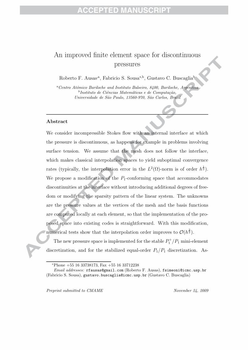
Accepted Manuscript
An improved finite element space for discontinuous pressures
Roberto F. Ausas, Fabricio S. Sousa, Gustavo C. Buscaglia
PII: S0045-7825(09)00386-7
DOI: 10.1016/j.cma.2009.11.011
Reference: CMA 9096
To appear in: Comput. Methods Appl. Mech. Engrg.
Received Date: 12 August 2009
Revised Date: 29 October 2009
Accepted Date: 16 November 2009
Please cite this article as: R.F. Ausas, F.S. Sousa, G.C. Buscaglia, An improved finite element space for
discontinuous pressures, Comput. Methods Appl. Mech. Engrg. (2009), doi: 10.1016/j.cma.2009.11.011
This is a PDF file of an unedited manuscript that has been accepted for publication. As a service to our customers
we are providing this early version of the manuscript. The manuscript will undergo copyediting, typesetting, and
review of the resulting proof before it is published in its final form. Please note that during the production process
errors may be discovered which could affect the content, and all legal disclaimers that apply to the journal pertain.
ACCEPTED MANUSCRIPT
An improved finite element space for discontinuous
pressures
Roberto F. Ausas,a, Fabricio S. Sousa∗,b, Gustavo C. Buscagliab
aCentro Atomico Bariloche and Instituto Balseiro, 8400, Bariloche, ArgentinabInstituto de Ciencias Matematicas e de Computacao,
Universidade de Sao Paulo, 13560-970, Sao Carlos, Brazil
Abstract
We consider incompressible Stokes flow with an internal interface at which
the pressure is discontinuous, as happens for example in problems involving
surface tension. We assume that the mesh does not follow the interface,
which makes classical interpolation spaces to yield suboptimal convergence
rates (typically, the interpolation error in the L2(Ω)-norm is of order h1
2 ).
We propose a modification of the P1-conforming space that accommodates
discontinuities at the interface without introducing additional degrees of free-
dom or modifying the sparsity pattern of the linear system. The unknowns
are the pressure values at the vertices of the mesh and the basis functions
are computed locally at each element, so that the implementation of the pro-
posed space into existing codes is straightforward. With this modification,
numerical tests show that the interpolation order improves to O(h3
2 ).
The new pressure space is implemented for the stable P+1 /P1 mini-element
discretization, and for the stabilized equal-order P1/P1 discretization. As-
∗Phone +55 16 33738173, Fax +55 16 33712238Email addresses: [email protected] (Roberto F. Ausas), [email protected]
(Fabricio S. Sousa), [email protected] (Gustavo C. Buscaglia)
Preprint submitted to CMAME November 24, 2009
ACCEPTED MANUSCRIPT
sessment is carried out for Poiseuille flow with a forcing surface and for a
static bubble. In all cases the proposed pressure space leads to improved
convergence orders and to more accurate results than the standard P1 space.
In addition, two Navier-Stokes simulations with moving interfaces (Rayleigh-
Taylor instability and merging bubbles) are reported to show that the pro-
posed space is robust enough to carry out realistic simulations.
Key words: Finite elements, interface, interpolation, discontinuous
pressure, surface tension
1. Introduction
Though much progress has been made over the last years in the field of
finite-element-based computational fluid mechanics, the accurate simulation
of flows with significant surface tension effects remains a challenge. This is
a consequence of two main difficulties that are inherent to such flows:
(i) The surface tension force FΓ is a surface Dirac distribution over the
interface Γ, proportional to the curvature of Γ. The singularity of the
force, together with its dependence of second derivatives of the interface
shape, renders it difficult to approximate.
(ii) Some of the flow variables, most importantly the pressure, are discontin-
uous across Γ. This leads to suboptimal interpolation accuracy when-
ever the finite element interpolants are continuous across Γ.
In a recent careful study, Gross and Reusken [1, 2] (see also [3]), have
shown that both of the aforementioned difficulties need to be specifically
2
ACCEPTED MANUSCRIPT
addressed or otherwise the convergence is poor (of order h1
2 in the L2(Ω)-
norm). In this article the attention is focused in difficulty (ii), for which
Gross and Reusken propose to adopt an XFEM [4] enrichment of the pressure
space, incorporating functions that are discontinuous at Γ, as had been also
proposed by Minev et al [5]. With this modification, they are able to get
improved convergence behavior, at the expense of the well-known pitfalls
of the XFEM methodology: The ill-conditioning of the system matrix due
to approximate linear dependence of the basis, and the introduction of new
unknowns that depend on the location of the interface, thus requiring the
code to completely rebuild the linear system structure for each interface
location.
Similar considerations have been made recently by Ganesan et al [6].
They compare mixed finite elements with continuous and discontinuous ap-
proximations for the pressure, and end up recommending the use of meshes
that follow the interface together with discontinuous pressure interpolants.
Clearly, this is the only combination of classical finite elements that yields a
pressure space that is discontinuous at Γ, which is the key to properly tackle
difficulty (ii) above. However, in a dynamic simulation it is cumbersome and
sometimes impossible to maintain the mesh aligned with the interface, so
that other remedies must be sought.
In this article we introduce a novel pressure space which accommodates
discontinuities at the (given) interface Γ, which is approximated by piecewise-
linear segments in 2D and piecewise-planar facets in 3D. The proposed space
is nothing but the classical conforming P1 space, locally modified at those
elements that are cut by the interface (which will be denoted as interface
3
ACCEPTED MANUSCRIPT
elements). The modification is local, computed element-by-element, and it
does not introduce any additional degrees of freedom. It is thus extremely
easy to incorporate the proposed space into existing codes. Further, the
only discontinuities take place at Γ, so that no special treatment is needed
at other interfaces (such as element-to-element interfaces, for example, as
happens with Discontinuous Galerkin methods).
The proposed pressure space will be introduced in the framework of the
(two-dimensional for simplicity) problem
−µ∇2u + ∇p = FΓ in Ω (1)
∇ · u = 0 in Ω (2)
u = 0 on ∂Ω (3)
where FΓ = f δΓ n, with f a given function, δΓ the Dirac delta distribution
on the line Γ, and n its normal. The singular force FΓ acts in fact as a jump
condition on the normal stress across Γ, namely,s−p + 2µ
∂un
∂n
= f, (4)
whereas both the velocity and the tangential stress remain continuous. In
fact, in this constant-viscosity case the velocity gradient exhibits no jump
across Γ [2], so that (4) reduces to JpK = −f . Notice that this simplified
model also represents the so-called actuator-disk model that is very popular
in the analysis of rotors (propellers, wind turbines, etc.) [7, 8, 9, 10, 11].
Denoting by V = H10 (Ω) × H1
0 (Ω) and Q = L2(Ω)/R, the variational
formulation that corresponds to (1)-(3) reads: “Find (u, p) ∈ V × Q such
that∫
Ω
[
µ(∇u + ∇T u) : ∇v − p ∇ · v + q ∇ · u]
dΩ =
∫
Γ
f n · v dΓ (5)
4
ACCEPTED MANUSCRIPT
for all (v, q) ∈ V × Q”. The bilinear and linear forms associated to the
variational formulation will be denoted by B(·, ·) and L(·), so that (5) can
be rewritten as
B((u, p), (v, q)) = L(v, q). (6)
Under reasonable regularity assumptions on Γ and f this problem admits a
unique solution, since it is only necessary that L be a bounded linear func-
tional. The finite element discretization of (5) is briefly recalled in Section
2, together with the description of the proposed pressure space. Section
3 contains several numerical experiments that assess the advantages of the
proposed space with respect to classical spaces. Some conclusions are finally
drawn in Section 4.
2. Finite element approximation
2.1. Galerkin mini-element formulation
In the Galerkin formulation, the exact variational formulation is restricted
to the space Vh×Qh, where Vh ⊂ V and Qh ⊂ Q are the approximation spaces
for velocity and pressure, respectively. The discrete formulation thus reads
“Find (uh, ph) ∈ Vh × Qh such that
B((uh, ph), (vh, qh)) = L(vh, qh) (7)
for all (vh, qh) ∈ Vh × Qh”. As is well-known, for this formulation to be
well-posed and convergent it is sufficient that the Babuska-Brezzi stability
condition[12, 13] be satisfied:
infqh ∈Qh
supvh ∈Vh
∫
Ωqh ∇ · vh dΩ
‖qh‖Q ‖vh‖V
≥ β > 0 (8)
5
ACCEPTED MANUSCRIPT
with β a mesh-independent constant.
The pressure and velocity spaces that correspond to the so-called mini-
element [14] are, for a finite element mesh Th:
Qh = Q1h := qh ∈ Q ∩ C0(Ω), qh|K ∈ P1(K), ∀K ∈ Th (9)
Vh = V mini
h := vh ∈ V, vh|K ∈ (P1(K) ⊕ span(bK))2 , ∀K ∈ Th (10)
where bK is the cubic bubble function that vanishes on all three edges of K.
Notice that the pressure space is nothing but the usual continuous P1 space,
while the space for each velocity component has been enriched by the bubble
functions so as to satisfy the stability condition. Being stable, this element
satisfies the a priori estimate
‖u − uh‖V + ‖p − ph‖Q ≤ C
(
infwh ∈Vh
‖u − wh‖V + infrh ∈Qh
‖p − rh‖Q
)
(11)
where C does not depend on the mesh size h. In the case of a smooth so-
lution, there exists a constant c such that infwh ∈Vh‖u − wh‖V ≤ c h |u|H2(Ω)
whereas infrh ∈Qh‖p − rh‖Q ≤ c h2 |p|H2(Ω). In the case of non-smooth so-
lutions involving pressure jumps, however, the latter interpolation estimate
deteriorates significantly [2], to
infrh ∈Qh
‖p − rh‖Q ≤ C(
h1
2 ‖JpK‖L∞(Γ) + h2 ‖p‖H2(Ω\Γ)
)
This approximation error of order h1
2 is a direct consequence of the pressure
interpolants being continuous across Γ, so that switching to discontinuous-
pressure elements does not cure it, unless the mesh follows the interface.
2.2. A discontinuous pressure space with the same unknowns
The proposed variant of the mini-element combines the velocity space
V mini
h (Eq. 10) with a new pressure space QΓh discussed below, without any
6
ACCEPTED MANUSCRIPT
modification of the Galerkin formulation (7).
2.2.1. The finite element interpolant
Let us now propose a different finite element space, denoted by QΓh, which
has the same unknowns as the conforming P1 space Q1h but admits disconti-
nuities across Γ. For all elements not cut by Γ standard P1 interpolants are
chosen. The only modifications appear in interface elements.
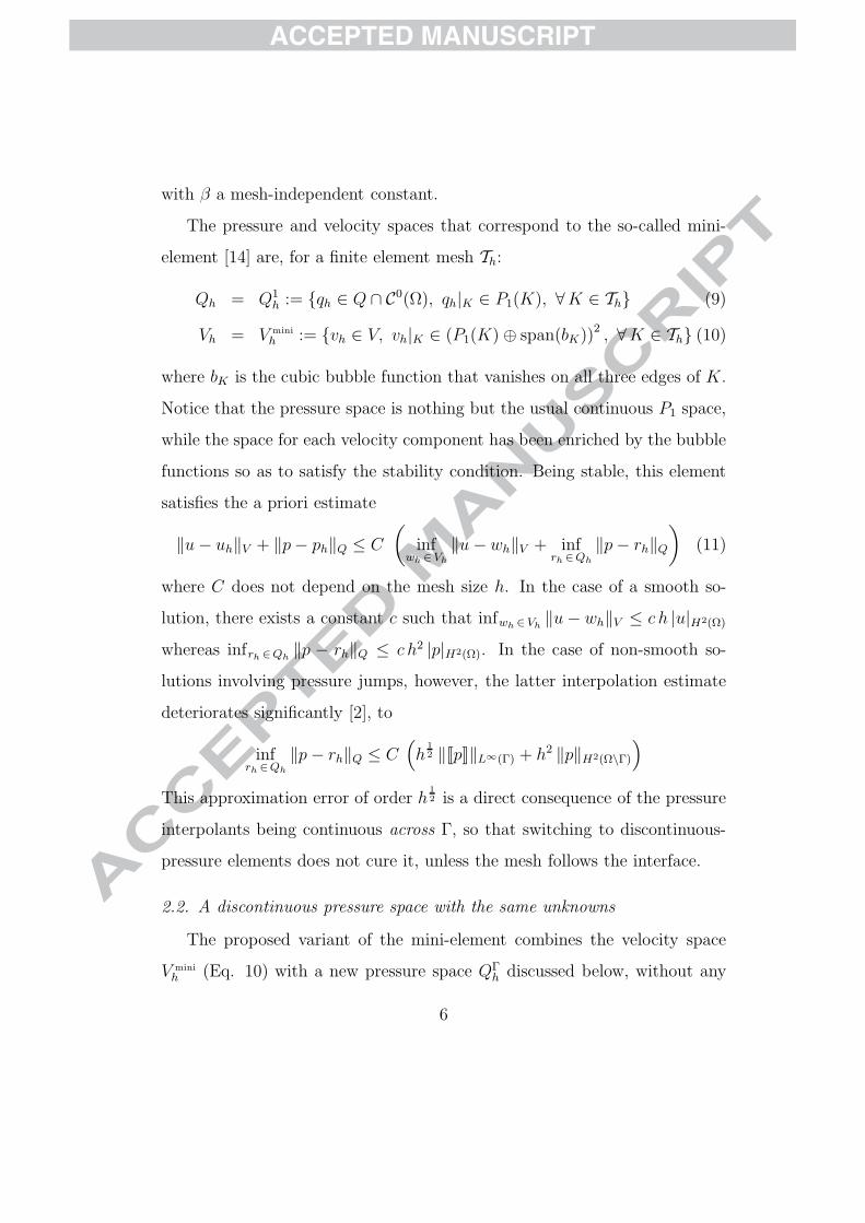
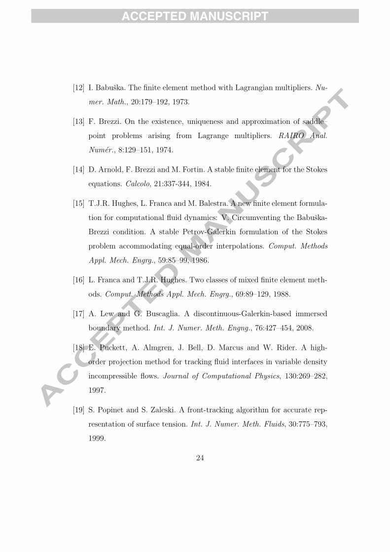
Consider the triangle ABC, which is cut by Γ into subtriangle APQ and
subquadrilateral BCQP (see Fig. 1). We assume for simplicity that, locally,
Γ is approximated by linear segments (this would probably add an additional
error of order h2, much smaller than the other errors involved). Let pA, pB,
pC denote the nodal values of the discrete pressure ph, to be interpolated in
the triangle ABC.
Let us arbitrarily denote the triangle APQ the “green” side of Γ and
quadrilateral BCQP the “red” side. For the approximation to be discontin-
uous, the function ph on the green side needs to be solely determined by the
only green node, i.e., A. Similarly, ph on the red side must depend on just
pB and pC . To accomplish this, we simply “carry” the value at each node
towards the intersection of any edge emanating from it with the interface.
In this way, on the green side of Γ, the values at P and Q will be pA, and
thus ph will be constant:
ph|APQ = pA
On the red side, the value at P will be pB and the value at Q will be pC . One
can here choose either to adopt a Q1 interpolation in BCQP from these nodal
values, or subdivide the quadrilateral into two triangles, BCP and CQP . In
any case, since the nodal values are given, the interpolation is immediate.
7
ACCEPTED MANUSCRIPT
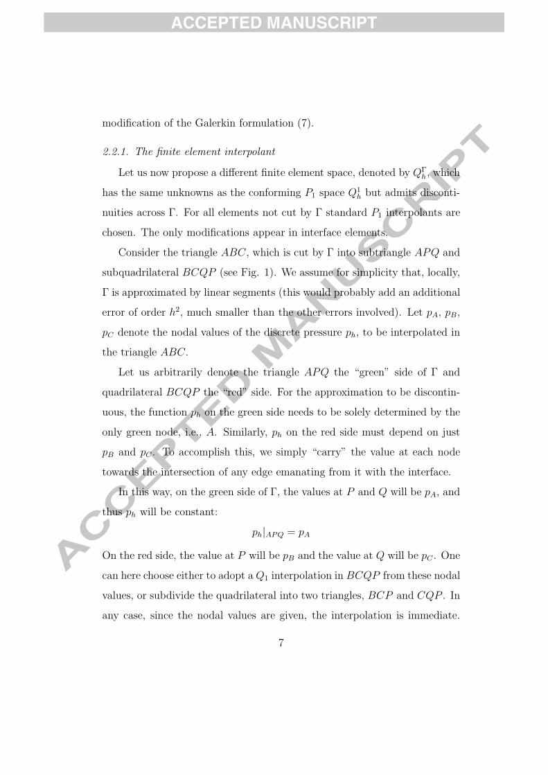
For the red triangle CQP , for example, ph will be the linear function that
takes the value pC at vertex C, the value pC at vertex Q, and the value pB at
vertex P . Notice that this interpolation leads to ph being discontinuous only
at Γ, since the function ph restricted to any edge of the triangle is uniquely
determined by the values at the nodes lying at the endpoints of that edge.
As a consequence of carrying the nodal values towards the intersection of
each edge with the interface, the space QΓh consists of functions with locally
an oblique derivative (in the direction of the edge that happens to cross Γ at
each point) equal to zero. The interpolation error ‖p−Ihp‖Q is thus expected
to be of order h3
2 for arbitrary p ∈ W 1,∞(Ω \ Γ).
Remark: It could be interesting to modify the proposed space in such a way
as to obtain an interpolation order of h2 for functions with any derivative
at Γ. A suitable way to do this would be by extrapolation along the edge
using some recovered gradient at the nodes. This is an operation that cannot
be carried out at the element level alone, and has not been explored in this
work.
Remark: Some modifications are needed if the interface Γ ends within the
domain (i.e., a cracked domain). Consider that the interface ends at some
point T that lies between P and Q, so that the segment TQ is not contained in
Γ. In this case the value of ph at Q is computed by linearly interpolating the
values pA and pC along the edge AC. The treatment of the intersection point
P is as before, so that the interpolant is continuous at Q and discontinuous
at P .
The extension of the proposed methodology to three dimensions follows
the lines described above. For completeness, the basis functions are given
8
ACCEPTED MANUSCRIPT
explicitly for the different possible cases in the paragraphs that follow.
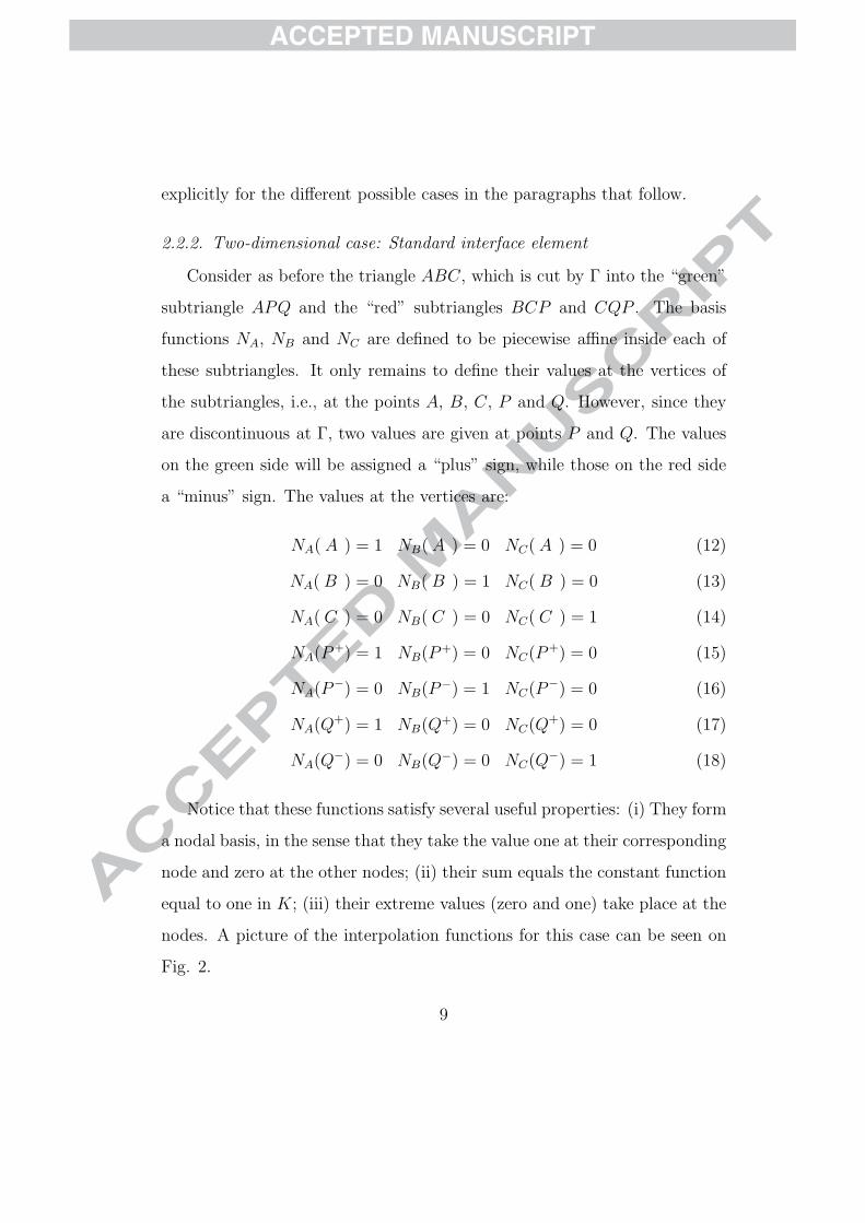
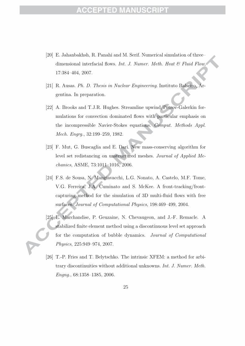
2.2.2. Two-dimensional case: Standard interface element
Consider as before the triangle ABC, which is cut by Γ into the “green”
subtriangle APQ and the “red” subtriangles BCP and CQP . The basis
functions NA, NB and NC are defined to be piecewise affine inside each of
these subtriangles. It only remains to define their values at the vertices of
the subtriangles, i.e., at the points A, B, C, P and Q. However, since they
are discontinuous at Γ, two values are given at points P and Q. The values
on the green side will be assigned a “plus” sign, while those on the red side
a “minus” sign. The values at the vertices are:
NA( A ) = 1 NB( A ) = 0 NC( A ) = 0 (12)
NA( B ) = 0 NB( B ) = 1 NC( B ) = 0 (13)
NA( C ) = 0 NB( C ) = 0 NC( C ) = 1 (14)
NA(P+) = 1 NB(P+) = 0 NC(P+) = 0 (15)
NA(P−) = 0 NB(P−) = 1 NC(P−) = 0 (16)
NA(Q+) = 1 NB(Q+) = 0 NC(Q+) = 0 (17)
NA(Q−) = 0 NB(Q−) = 0 NC(Q−) = 1 (18)
Notice that these functions satisfy several useful properties: (i) They form
a nodal basis, in the sense that they take the value one at their corresponding
node and zero at the other nodes; (ii) their sum equals the constant function
equal to one in K; (iii) their extreme values (zero and one) take place at the
nodes. A picture of the interpolation functions for this case can be seen on
Fig. 2.
9
ACCEPTED MANUSCRIPT
Remark: Though unlikely in practical cases, it could happen that Γ passes
exactly through a vertex. This is a degenerate case in which one of the
subtriangles becomes a needle of vanishingly small volume.
2.2.3. Two-dimensional case: Element containing an interface endpoint
In the case that Γ has an endpoint at element K, special basis functions
are needed. Consider P to be the last edge-interface intersection point, and
T to be the interface endpoint (see Figure 3). The point Q is defined as
the intersection of the line PT with the edge AC. The difference with the
previous case is that now the functions need to be continuous at point Q.
For this purpose, let g be an affine function defined on the edge AC such
that g(A) = 1 and g(C) = 0 (in other words, g is the restriction to edge AC
of the P1 basis function corresponding to node A). The values of NA, NB
and NC at points A, B, C, P+ and P− are as in (12)-(16). At point Q the
functions are continuous, with values
NA(Q) = g(Q), NB(Q) = 0, NC(Q) = 1 − g(Q) (19)
Properties (i)-(iii) above are also satisfied by this basis. An illustration
of these functions can be seen on Fig. 4.
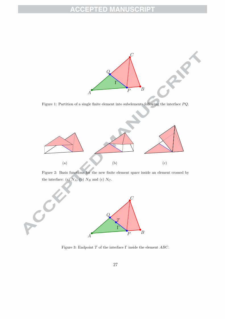
2.2.4. Three-dimensional case: Standard interface element
Consider that the element K cut by the interface is the tetrahedron
ABCD as shown in Fig. 5, of which either three (case (a)) or four (case
(b)) edges are cut by Γ.
In case (a), there appear three intersection points P , Q and R (see Fig.
5(a)), at which the nodal functions NA, NB, NC and ND are bi-valued. As
10

ACCEPTED MANUSCRIPT
in the two-dimensional case, the plus and minus values at the intersection
points correspond to the “green” and “red” sides of the interface. Carrying
the values to the interface as explained, the values of the basis functions at
the vertices and intersection points are:
NA( A ) = 1, NB( A ) = 0, NC( A ) = 0, ND( A ) = 0 (20)
NA( B ) = 0, NB( B ) = 1, NC( B ) = 0, ND( B ) = 0 (21)
NA( C ) = 0, NB( C ) = 0, NC( C ) = 1, ND( C ) = 0 (22)
NA( D ) = 0, NB( D ) = 0, NC( D ) = 0, ND( D ) = 1 (23)
NA(P+) = 1, NB(P+) = 0, NC(P+) = 0, ND(P+) = 0 (24)
NA(P−) = 0, NB(P−) = 1, NC(P−) = 0, ND(P−) = 0 (25)
NA(Q+) = 1, NB(Q+) = 0, NC(Q+) = 0, ND(Q+) = 0 (26)
NA(Q−) = 0, NB(Q−) = 0, NC(Q−) = 1, ND(Q−) = 0 (27)
NA(R+) = 1, NB(R+) = 0, NC(R+) = 0, ND(R+) = 0 (28)
NA(R−) = 0, NB(R−) = 0, NC(R−) = 0, ND(R−) = 1 (29)
The truncated tetrahedron BCDPQR is divided into subtetrahedra and
from the values at the vertices given above the basis functions are obtained
by affine interpolation over each subtetrahedron. Satisfaction of 3D analogs
of properties (i)-(iii) is straightforward. In this case, for the resulting inter-
polant not to be discontinuous at the faces (outside Γ) the neighbor element
must be subdivided in a compatible way. For face ABC, for example, conti-
nuity of NB and NC is only obtained if both elements sharing this face divide
the quadrilateral BCPQ by the same diagonal.
In case (b) there appear four intersection points, namely P , Q, R and
11
ACCEPTED MANUSCRIPT
S (see Fig. 5(b)). The values of the basis functions at A, B, C and D are
obviously the same as in (20)-(23). The values at the intersection points
follow the same procedure as before, yielding
NA(P+) = 1, NB(P+) = 0, NC(P+) = 0, ND(P+) = 0 (30)
NA(P−) = 0, NB(P−) = 0, NC(P−) = 1, ND(P−) = 0 (31)
NA(Q+) = 1, NB(Q+) = 0, NC(Q+) = 0, ND(Q+) = 0 (32)
NA(Q−) = 0, NB(Q−) = 0, NC(Q−) = 0, ND(Q−) = 1 (33)
NA(R+) = 0, NB(R+) = 1, NC(R+) = 0, ND(R+) = 0 (34)
NA(R−) = 0, NB(R−) = 0, NC(R−) = 1, ND(R−) = 0 (35)
NA(S+) = 0, NB(S+) = 1, NC(S+) = 0, ND(S+) = 0 (36)
NA(S−) = 0, NB(S−) = 0, NC(S−) = 0, ND(S−) = 1 (37)
Properties (i)-(iii) are easily seen to hold, while continuity across the faces
again depends on the compatibility of the subdivisions between neighboring
elements.
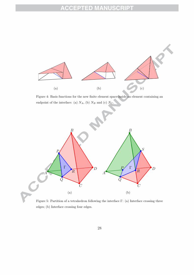
2.2.5. Three-dimensional case: Interface with boundary
If the interface Γ has a boundary ∂Γ within the domain, the basis func-
tions need to be modified in much the same way as in the two-dimensional
case. Let K be an element cut by the surface Γ and such that ∂Γ ∩ K 6= ∅.
We assume that Γ ∩ K is a planar polygon and thus the intersection of this
plane with the edges of K defines the points P , Q, R and, in a case-(b)
situation, S, as before.
Consider for example that the intersection is as shown in Fig. 6, so
that the subdivision corresponds to case (b). Notice, however, that the edge
12
ACCEPTED MANUSCRIPT
BD is not crossed by the interface, so that the basis functions must be
continuous along this edge and thus, in particular, at point S. Proceeding
as in the two-dimensional case, we assign to S a unique value provided by
the linear interpolation between nodes B and D. This procedure is adopted
for all intersection points falling outside Γ. Properties (i)-(iii) are easily seen
to hold, as well as continuity of the basis functions across the faces (again
depending on a compatible choice of diagonals for quadrilaterals).
2.3. A stabilized method
It is also possible to consider finite element formulations that do not
satisfy the Babuska-Brezzi condition (8), but are rendered convergent by
means of stabilization techniques [15, 16]. This is the case of the equal-order
P1/P1 formulation in which the discrete spaces are
Qh = Q1h (as before) (38)
Vh = V 1h := vh ∈ V, vh|K ∈ P1(K)2, ∀K ∈ Th (39)
and the formulation reads: “Find (uh, ph) ∈ Vh × Qh such that
B((uh, ph), (vh, qh)) +∑
K ∈Th
τK
∫
K
R(uh, ph) · ∇qh dK = L(vh, qh) (40)
for all (vh, qh) ∈ Vh × Qh”. The stabilization coefficient τK is taken as
τK =h2
K
4µ
where hK is the element size, and the residual is defined as
R(uh, ph) = −µ∇2uh + ∇ph − FΓ. (41)
13
ACCEPTED MANUSCRIPT
For regular forces (e.g., forces in L2(Ω), which is not the case of FΓ), it is
possible to prove an error estimate [16] which is essentially equivalent to (11).
To our knowledge, no analysis exists of stabilized methods in problems
involving singular forces. Our approach is to set τK to zero whenever the
element K is cut by the interface. Though this could potentially lead to lack
of stability, no spurious pressure modes were detected in any of the numerical
tests. We attribute this to the band-like structure of the submesh in which
the stabilization is omitted, which is too narrow (just one band of elements)
for spurious modes to develop. In a different context, Lew and Buscaglia [17]
observed that switching the elements crossed by Γ to a discontinuous Galerkin
discretization required no stabilization, though the same space indeed requires
stabilization when used in the whole domain.
3. Numerical experiments
In this section we carry out numerical assessments of the proposed space.
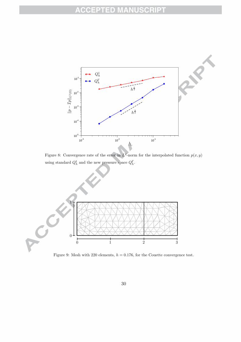
We first investigate the interpolation accuracy of the space QΓh and indeed
obtain the claimed h3
2 -order in the L2(Ω)-norm. Then we turn to academic
Navier-Stokes tests with analytic solution in which QΓh is used as pressure
space. These tests show that the new space does not deteriorate the stability
properties of either the stable mini-element formulation or the stabilized
equal-order formulation. Finally, two more realistic problems are simulated
to show that the proposed method is robust enough to handle arbitrarily
moving interfaces in two and three dimensions.
14
ACCEPTED MANUSCRIPT
3.1. Interpolation properties of the space QΓh
We first assess purely the interpolation properties of QΓh. For this pur-
pose we perform tests similar to those conducted by Reusken [3]. Let Ω =
(−π2, π
2) × (−π
2, π
2) and let Γ = (x, y) ∈ Ω | x = 0 , y > 0. Let p be the
function
p(x, y) =
e−x sin2(y) if (x > 0 and y > 0)
0 otherwise. (42)
Notice that Γ is a “crack” in the domain, and that p is discontinuous across
Γ.
The interpolant Ihp of p is now defined as the unique element of QΓh that
coincides with p at all the vertices of Th.
A sequence of unstructured meshes was built, of which the first one is
shown in Fig. 7. To this mesh, which consists of 326 triangles, we assign
a mesh size of h = 0.2. The following meshes in the sequence are built by
successively dividing each of the triangles of the previous mesh into four equal
triangles, leading to meshes with h = 0.1, h = 0.05 and so forth, until the
finest mesh with h = 3.125 × 10⁻³.
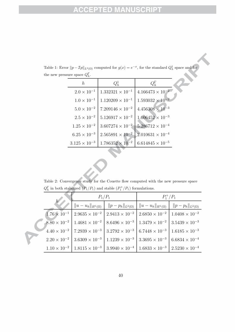
We measured the error of p − Ihp in the L2(Ω)-norm. The results are
shown in Table 1, in which we also include the interpolation error of the
P1-conforming interpolant for comparison (Q1h). Figure 8 displays the con-
vergence rate of the order of h3
2 .
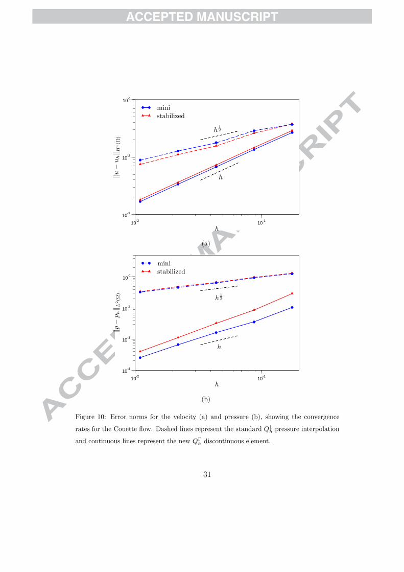
3.2. Couette flow
In this experiment we consider the domain [0, L] × [0, H ], with periodic
boundary conditions in the x1-direction. The velocity is set to zero at the
15
ACCEPTED MANUSCRIPT
top and bottom boundaries
u(x1, x2 = 0) = u(x1, x2 = H) = 0
and the interface Γ is a straight vertical line x1 = a, on which a constant
unit normal force f = 1 is imposed. The exact solution for this problem is
u1(x1, x2) =1
2µLx2 (H − x2) (43)
u2(x1, x2) = 0 (44)
p(x1, x2) = −1
Lx1 + H(x1 − a) (45)
where H(x1 − a) = 1 if x1 > a and zero otherwise, and the indeterminacy
of the pressure was removed by imposing p(0, 0) = 0 instead of setting the
average to zero, for simplicity.
This problem, with L = 3, H = 1, µ = 1 and a = 2 was discretized both
with the mini-element and with the stabilized equal-order methods. In both
cases, the classical P1-conforming pressure space (denoted by Q1h above) and
the new space QΓh were implemented.
As in the previous section, a sequence of unstructured meshes was built,
of which the first one is shown in Fig. 9. To this mesh, which consists of
220 triangles, we assign a mesh size of h = 0.176. The following meshes in
the sequence are built by subdivision. We measure the velocity error in the
H1(Ω)-norm and the pressure error in the L2(Ω)-norm for both methods as
functions of h. The results of the convergence analysis are displayed in Table
2 and Fig. 10. The experimental orders of convergence are
‖u − uh‖H1(Ω) = O(h1
2 ), ‖p − ph‖L2(Ω) = O(h1
2 )
16
ACCEPTED MANUSCRIPT
for the standard Q1h space; and
‖u − uh‖H1(Ω) = O(h), ‖p − ph‖L2(Ω) = O(h)
for the proposed method. The optimal convergence of smooth problems is
thus recovered with the proposed modification of the pressure space.
The pressure field corresponding to the classical mini-element is compared
to that obtained with the proposed method in Fig. 11. As is clear from the
figure, the improved pressure space exhibits significantly smaller pressure
oscillations near the interface than the mini-element.
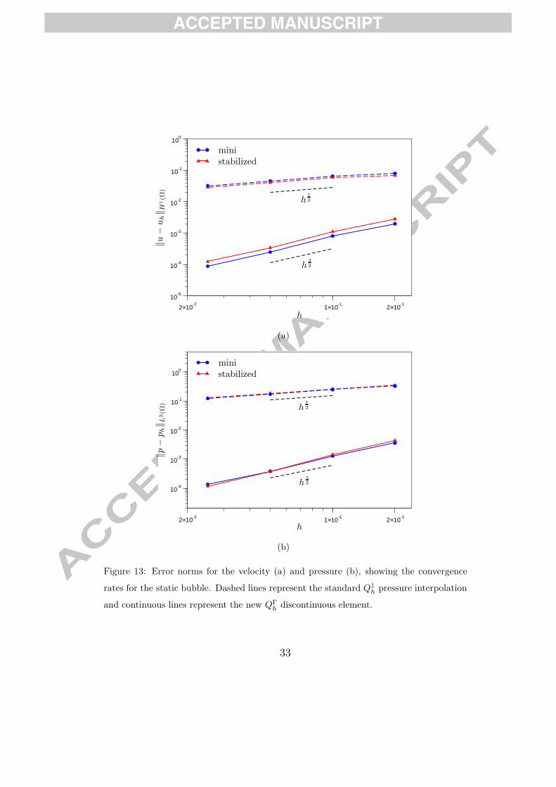
3.3. Static two-dimensional bubble
The second example we report here concerns a 2D static bubble. In this
case the interface Γ is the circle of radius R centered at the origin. On Γ, a
constant (inwards) normal force is imposed, f = σR, where σ represents the
surface tension. Setting the pressure outside the bubble arbitrarily to zero,
the exact pressure inside the bubble equals σR. The exact velocity vanishes
everywhere.
In this example we approximate Γ by Γh, which consists of straight seg-
ments inside each element that join the intersections of Γ with the element
edges (i.e., the points P and Q are joined by a straight segment). With Γh
fixed, we impose the surface tension force in two ways:
Direct forcing: We impose
FΓ = −σ
RδΓh
er (46)
where er is the radial unit vector, leading to
L(vh, qh) = −σ
R
∫
Γh
er · vh dΓ (47)
17
ACCEPTED MANUSCRIPT
Laplace-Beltrami forcing: The Laplace-Beltrami treatment of surface ten-
sion is based on the identity (valid for a closed surface of curvature κ)
∫
Γ
κ n · v dΓ = −
∫
Γ
(I − n⊗ n) : ∇v dΓ (48)
where I is the identity tensor, the symbol ⊗ denotes the tensor product,
and “:” stands for the double contraction of rank two tensors. This
leads to the following linear form on the right-hand side of (7) and/or
(40):
L(vh, qh) = − σ
∫
Γh
(I − nh ⊗ nh) : ∇vh dΓ (49)
where nh is the unit normal to Γh.
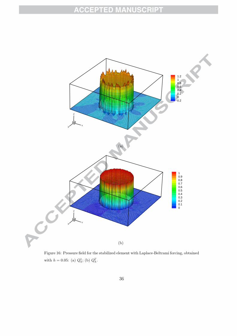
For the numerical tests we chose R = µ = σ = 1, and the domain was set
to Ω = (−2, 2)× (−2, 2). The velocity is set to zero on ∂Ω, and the pressure
at the left bottom corner of the domain is set to zero to fully determine the
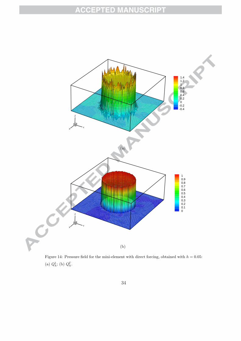
pressure. We present results for the mini-element formulation with direct
forcing (ME+DF), and for the stabilized formulation with Laplace-Beltrami
forcing (ST+LB). A mesh refinement study was conducted in the same way
as in the previous examples, starting with the mesh shown in Fig. 12, to
which we assign h = 0.2. Logarithmic plots of the velocity and pressure
errors are shown in Fig. 13. Clearly, both methods converge with order
O(h1
2 ) if the standard pressure space Q1h is used, while switching to QΓ
h
improves the order to O(h3
2 ). The obtained pressure and velocity fields on
the mesh with h = 0.05, which consists of 14900 elements, are shown in
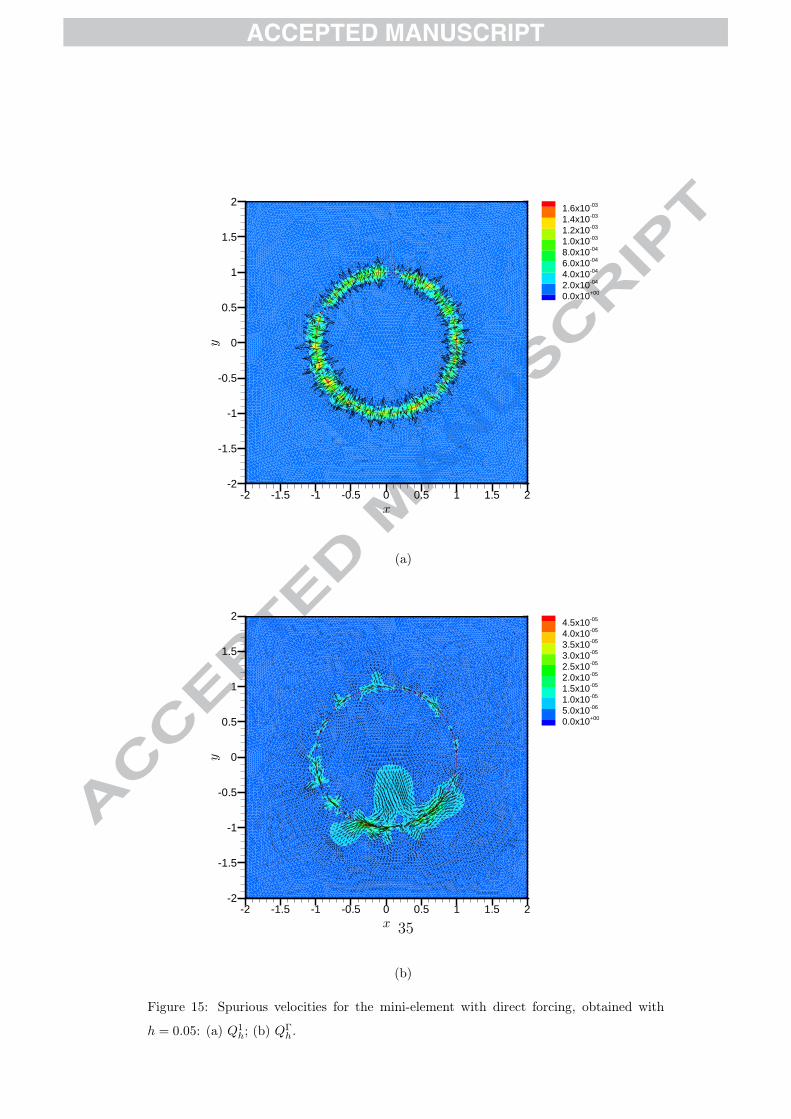
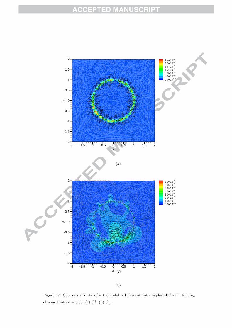
Figs. 14 and 15 for the ME+DF formulation, and in Figs. 16 and 17 for the
ST+LB formulation. The improvements brought by the proposed method are
evident. The parasitic velocities obtained with the ME+DF formulation have
18
ACCEPTED MANUSCRIPT
a maximum modulus of 1.6 × 10⁻³ when the P1 space is used for pressure,
whereas with the proposed space this value is much smaller (4.5 × 10⁻⁵).
Similarly, in the ST+LB formulation the maximum velocity modulus is 2.4×
10−3 for Q1h and 7 × 10⁻⁵ for QΓ
h .
3.4. Rayleigh-Taylor instability
This is a well-known benchmark which has been computed by Puckett et
al [18], Popinet and Zaleski [19] and Jahanbakhsh et al [20], among others.
It consists of a layer of heavier fluid (ρ = 1.225) on top of a lighter fluid (ρ =
0.1694), both with viscosity µ = 3.13 × 10⁻². The domain is the rectangle
Ω = (0, 1)× (0, 4) and the gravity is taken as g = 10. The interface between
the fluids is a horizontal line with a sinusoidal perturbation of amplitude 0.05.
We consider the standard case, with no surface tension, and also simulate a
case with σ = 0.025 in which the ability of the numerical method to reproduce
the stabilizing effect of surface tension is tested.
To carry out this simulation (and the one in the next subsection) the
proposed pressure space was incorporated into a general purpose in-house
interface-capturing code that simulates fluids with evolving interfaces. The
details of the code are explained elsewhere [21]. Let us here simply summarize
its basic ingredients:
• Stabilized equal-order formulation of the time-dependent Navier-Stokes
equations.
• Level set formulation for interface representation and transport. Stan-
dard P1 conforming elements for the level set function φ. The transport
19
ACCEPTED MANUSCRIPT
of φ is handled with the SUPG method [22], with mass-preserving pe-
riodic reinitialization as proposed by Mut et al [23].
• Laplace-Beltrami treatment of the surface tension force.
Numerical results at several times, as computed on a uniform mesh con-
sisting of 331,776 elements with a time step ∆t = 6.25 × 10⁻⁴ are shown in
Fig. 18. The results with σ = 0 are in good agreement with those reported
by Jahanbakhsh et al [20], while the stabilizing effect of surface tension is
clear from the simulation results with σ = 0.025.
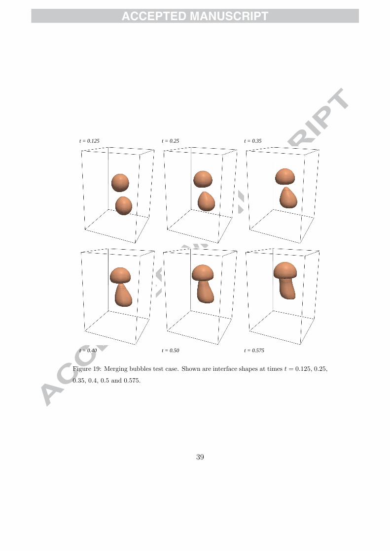
3.5. Merging bubbles
This experiment shows the good behavior of the proposed method in
three-dimensional complex cases. We study the rise of two buoyant bubbles
(ρ = 0.04, µ = 5 × 10⁻³) in a quiescent liquid with ρ = 1 and µ = 0.1. The
diameter of the bubbles is 1 and the domain is Ω = (0, 3) × (0, 3) × (0, 4).
The gravity is g = 10, the surface tension σ = 0.2 and the initial positions
of the bubbles’ centers are (1.5, 1.5, 2.25) and (1.5, 1.75, 1) (notice that they
are not vertically aligned).
The finite element mesh consists of 885,000 tetrahedra, and the time step
is taken as 10−3. Shown in Fig. 19 is the interface shape at times t = 0.125,
0.25, 0.35, 0.4, 0.5 and 0.575. The bottom bubble follows and catches the
top one, and the results are in good agreement with those reported by Sousa
et al [24] and Marchandise et al [25].
20
ACCEPTED MANUSCRIPT
4. Conclusions
A new finite element space QΓh has been proposed, which has the same un-
knowns as the P1-conforming space but consists of functions that are discon-
tinuous across a given interface Γ, assumed not aligned with the mesh. The
proposed space is much simpler than the one proposed by Gross and Reusken
[2], which is based on XFEM enrichment, and also to the one proposed by
Fries and Belytschko [26], which avoids introducing additional unknowns by
switching to a moving-least-squares approximation in the vicinity of Γ.
Through numerical tests it was shown that the L2(Ω)-interpolation ac-
curacy of QΓh for functions that are smooth outside Γ is O(h
3
2 ). This is a
significant improvement with respect to the accuracy of continuous spaces of
any polynomial degree, which is O(h1
2 ).
An interpolation accuracy of O(h3
2 ) in the L2(Ω)-norm is suboptimal for
piecewise linear elements. However, the a priori estimate (11) implies that
the space QΓh , when taken as pressure space, will not limit the accuracy of a
(Navier-)Stokes calculation neither in equal-order velocity-pressure approxi-
mations, nor in the mini-element approximation. In fact, in both cases the
global accuracy is limited by the H1(Ω)-accuracy of the velocity space, which
is O(h).
The proposed space is easy to implement, requiring just local operations
at the element level to incorporate the improved pressure interpolation. Sev-
eral tests were reported which illustrate the improved behavior of both ve-
locity and pressure when the elements cut by the interface are treated with
the proposed pressure interpolants.
Some issues are left for future work. A rigorous proof of the interpolation
21

ACCEPTED MANUSCRIPT
estimate has been undertaken by Agouzal and Buscaglia, of which some pre-
liminary results have already been communicated [27] and a complete version
is in preparation. Another open theoretical question concerns the stability
estimates for the Vh-QΓh pair, of which strong numerical evidence has been
provided in this article but whose proof is far from evident. Finally, it would
be interesting to devise spaces analog to QΓh when the overall discretization
is Pk-conforming with k > 1, but this is, again, far from being an immediate
extension of the space proposed in this article.
ACKNOWLEDGMENTS: The authors acknowledge partial support from
FAPESP (Brazil), CNPq (Brazil), CNEA (Argentina) and CONICET (Ar-
gentina). This research was carried out in the framework of INCT-MACC,
Ministerio de Ciencia e Tecnologia, Brazil.
References
[1] S. Gross and A. Reusken. Finite element discretization error analysis
of a surface tension force in two-phase incompressible flows. SIAM J.
Numer. Anal., 45:1679–1700, 2007.
[2] S. Gross and A. Reusken. An extended pressure finite element space for
two-phase incompressible flows with surface tension. Journal of Com-
putational Physics, 224:40–58, 2007.
[3] A. Reusken. Analysis of an extended pressure finite element space for
two–phase incompressible flows. Comput. Visual. Sci., 11:293–305, 2008.
[4] T. Belytschko, N. Moes, S. Usui, and C. Parimi. Arbitrary disconti-
22
ACCEPTED MANUSCRIPT
nuities in finite elements. Int. J. Numer. Meth. Engng, 50:993–1013,
2001.
[5] P.D. Minev, T. Chen, and K. Nandakumar. A finite element technique
for multifluid incompressible flow using Eulerian grids. Journal of Com-
putational Physics, 187:225–273, 2003.
[6] S. Ganesan, G. Matthies, and L. Tobiska. On spurious velocities in
incompressible flow problems with interfaces. Comput. Methods Appl.
Mech. Engrg., 196:1193–1202, 2007.
[7] R. Mikkelsen. Actuator disc methods applied to wind turbines. Ph. D.
Thesis MEK-FM-PHD 2003-02. Technical Univ. Denmark. June 2003.
[8] C. Meyer and D. Kroger. Numerical simulation of the flow field in the
vicinity of an axial flow fan. Int. J. Numer. Meth. Fluids, 36:947–969,
2001.
[9] Y. Tahara, R. Wilson, P. Carrica and F. Stern. RANS simulation of a
container ship using a single–phase level–set method with overset grids
and the prognosis for extension to a self–propulsion simulator. J. Marine
Sci. Technol., 11:209–228, 2006.
[10] P. Carrica, K.-J. Paik, H. Hosseini and F. Stern. URANS analysis of
a broaching event in irregular quartering seas. J. Marine Sci. Technol.,
13:395–407, 2008.
[11] C. Leclerc and C. Masson. Wind turbine performance predictions us-
ing a differential actuator–lifting disk model. J. Solar Energy Engng.,
127:200–208, 2005.
23
ACCEPTED MANUSCRIPT
[12] I. Babuska. The finite element method with Lagrangian multipliers. Nu-
mer. Math., 20:179–192, 1973.
[13] F. Brezzi. On the existence, uniqueness and approximation of saddle–
point problems arising from Lagrange multipliers. RAIRO Anal.
Numer., 8:129–151, 1974.
[14] D. Arnold, F. Brezzi and M. Fortin. A stable finite element for the Stokes
equations. Calcolo, 21:337-344, 1984.
[15] T.J.R. Hughes, L. Franca and M. Balestra. A new finite element formula-
tion for computational fluid dynamics: V. Circumventing the Babuska-
Brezzi condition. A stable Petrov-Galerkin formulation of the Stokes
problem accommodating equal-order interpolations. Comput. Methods
Appl. Mech. Engrg., 59:85–99, 1986.
[16] L. Franca and T.J.R. Hughes. Two classes of mixed finite element meth-
ods. Comput. Methods Appl. Mech. Engrg., 69:89–129, 1988.
[17] A. Lew and G. Buscaglia. A discontinuous-Galerkin-based immersed
boundary method. Int. J. Numer. Meth. Engng., 76:427–454, 2008.
[18] E. Puckett, A. Almgren, J. Bell, D. Marcus and W. Rider. A high-
order projection method for tracking fluid interfaces in variable density
incompressible flows. Journal of Computational Physics, 130:269–282,
1997.
[19] S. Popinet and S. Zaleski. A front-tracking algorithm for accurate rep-
resentation of surface tension. Int. J. Numer. Meth. Fluids, 30:775–793,
1999.
24
ACCEPTED MANUSCRIPT
[20] E. Jahanbakhsh, R. Panahi and M. Serif. Numerical simulation of three–
dimensional interfacial flows. Int. J. Numer. Meth. Heat & Fluid Flow,
17:384–404, 2007.
[21] R. Ausas. Ph. D. Thesis in Nuclear Engineering. Instituto Balseiro, Ar-
gentina. In preparation.
[22] A. Brooks and T.J.R. Hughes. Streamline upwind/Petrov-Galerkin for-
mulations for convection dominated flows with particular emphasis on
the incompressible Navier-Stokes equations. Comput. Methods Appl.
Mech. Engrg., 32:199–259, 1982.
[23] F. Mut, G. Buscaglia and E. Dari. New mass-conserving algorithm for
level set redistancing on unstructured meshes. Journal of Applied Me-
chanics, ASME, 73:1011–1016, 2006.
[24] F.S. de Sousa, N. Mangiavacchi, L.G. Nonato, A. Castelo, M.F. Tome,
V.G. Ferreira, J.A. Cuminato and S. McKee. A front-tracking/front-
capturing method for the simulation of 3D multi-fluid flows with free
surfaces. Journal of Computational Physics, 198:469–499, 2004.
[25] E. Marchandise, P. Geuzaine, N. Chevaugeon, and J.-F. Remacle. A
stabilized finite element method using a discontinuous level set approach
for the computation of bubble dynamics. Journal of Computational
Physics, 225:949–974, 2007.
[26] T.-P. Fries and T. Belytschko. The intrinsic XFEM: a method for arbi-
trary discontinuities without additional unknowns. Int. J. Numer. Meth.
Engng., 68:1358–1385, 2006.
25

ACCEPTED MANUSCRIPT
[27] G. Buscaglia and A. Agouzal. Interpolation estimate for a finite ele-
ment space with embedded discontinuities. In Proc. 30th Iberian-Latin-
American Congress on Computational Methods in Engineering, Buzios,
Brazil, November 8–11, 2009.
26
ACCEPTED MANUSCRIPT
AB
C
P
Q
Γ
Figure 1: Partition of a single finite element into subelements following the interface PQ.
(a) (b) (c)
Figure 2: Basis functions for the new finite element space inside an element crossed by
the interface: (a) NA, (b) NB and (c) NC .
AB
C
P
QT
Γ
Figure 3: Endpoint T of the interface Γ inside the element ABC.
27
ACCEPTED MANUSCRIPT
(a) (b) (c)
Figure 4: Basis functions for the new finite element space inside an element containing an
endpoint of the interface: (a) NA, (b) NB and (c) NC .
A
B
C
D
P
Q
RΓ
(a)
A
B
C
DP
Q
R
S
Γ
(b)
Figure 5: Partition of a tetrahedron following the interface Γ: (a) Interface crossing three
edges; (b) Interface crossing four edges.
28

ACCEPTED MANUSCRIPT
A
B
C
DP
Q
R
S
Γ
Figure 6: Partition of a tetrahedron K where ∂Γ ∩ K 6= ∅. Point S is obtained by
intersecting plane PQR with edge BD.
−π
2
−π
2
0
0
π
2
π
2
Figure 7: First mesh used in the interpolation test, with 326 elements. The interface Γ is
a line from (0,0) to (0,π
2 ).
29
ACCEPTED MANUSCRIPT
10-3
10-2
10-1
10-5
10-4
10-3
10-2
10-1
‖p−Ip‖ L
2(Ω
)
h
h3
2
h1
2
Q1h
QΓh
Figure 8: Convergence rate of the error in L2-norm for the interpolated function p(x, y)
using standard Q1h
and the new pressure space QΓh.
0
0
1
1 2 3
Figure 9: Mesh with 220 elements, h = 0.176, for the Couette convergence test.
30
ACCEPTED MANUSCRIPT
10-2
10-1
10-3
10-2
10-1
‖u−
uh‖ H
1(Ω
)
h
h1
2
h
ministabilized
(a)
10-2
10-1
10-4
10-3
10-2
10-1
‖p−
ph‖ L
2(Ω
)
h
h1
2
h
ministabilized
(b)
Figure 10: Error norms for the velocity (a) and pressure (b), showing the convergence
rates for the Couette flow. Dashed lines represent the standard Q1h
pressure interpolation
and continuous lines represent the new QΓh
discontinuous element.
31

ACCEPTED MANUSCRIPT
0 0,5 1 1,5 2 2,5 3
-0,8
-0,6
-0,4
-0,2
0
0,2
0,4
x
p hQΓ
h
Q1
h
Exact
Figure 11: Computed pressure using the stable formulation (mini-element), with standard
and new pressure space.
0
0
1
1
2
2
−1
−1
−2
−2
Figure 12: Mesh for the static bubble convergence study, with 1104 elements and h = 0.2.
32
ACCEPTED MANUSCRIPT
2×10⁻²
1×10⁻¹
2×10⁻¹
10-5
10-4
10-3
10-2
10-1
100
‖u−
uh‖ H
1(Ω
)
h
h1
2
h3
2
ministabilized
(a)
2×10⁻²
1×10⁻¹
2×10⁻¹
10-4
10-3
10-2
10-1
100
‖p−
ph‖ L
2(Ω
)
h
h1
2
h3
2
ministabilized
(b)
Figure 13: Error norms for the velocity (a) and pressure (b), showing the convergence
rates for the static bubble. Dashed lines represent the standard Q1h
pressure interpolation
and continuous lines represent the new QΓh
discontinuous element.
33
ACCEPTED MANUSCRIPT
XY
Z
1.41.210.80.60.40.20
-0.2-0.4
(a)
XY
Z
10.90.80.70.60.50.40.30.20.10
(b)
Figure 14: Pressure field for the mini-element with direct forcing, obtained with h = 0.05:
(a) Q1h; (b) QΓ
h.
34
ACCEPTED MANUSCRIPT
-2 -1.5 -1 -0.5 0 0.5 1 1.5 2-2
-1.5
-1
-0.5
0
0.5
1
1.5
21.6x10-03
1.4x10-03
1.2x10-03
1.0x10-03
8.0x10-04
6.0x10-04
4.0x10-04
2.0x10-04
0.0x10+00
x
y
(a)
-2 -1.5 -1 -0.5 0 0.5 1 1.5 2-2
-1.5
-1
-0.5
0
0.5
1
1.5
24.5x10-05
4.0x10-05
3.5x10-05
3.0x10-05
2.5x10-05
2.0x10-05
1.5x10-05
1.0x10-05
5.0x10-06
0.0x10+00
x
y
(b)
Figure 15: Spurious velocities for the mini-element with direct forcing, obtained with
h = 0.05: (a) Q1h; (b) QΓ
h.
35
ACCEPTED MANUSCRIPT
XY
Z
1.210.80.60.40.20
-0.2
(a)
XY
Z
10.90.80.70.60.50.40.30.20.10
(b)
Figure 16: Pressure field for the stabilized element with Laplace-Beltrami forcing, obtained
with h = 0.05: (a) Q1h; (b) QΓ
h.
36
ACCEPTED MANUSCRIPT
-2 -1.5 -1 -0.5 0 0.5 1 1.5 2-2
-1.5
-1
-0.5
0
0.5
1
1.5
2 2.4x10-03
2.0x10-03
1.6x10-03
1.2x10-03
8.0x10-04
4.0x10-04
0.0x10+00
x
y
(a)
-2 -1.5 -1 -0.5 0 0.5 1 1.5 2-2
-1.5
-1
-0.5
0
0.5
1
1.5
2 7.0x10-05
6.0x10-05
5.0x10-05
4.0x10-05
3.0x10-05
2.0x10-05
1.0x10-05
0.0x10+00
x
y
(b)
Figure 17: Spurious velocities for the stabilized element with Laplace-Beltrami forcing,
obtained with h = 0.05: (a) Q1h; (b) QΓ
h.
37
ACCEPTED MANUSCRIPT
t = 0.5 t = 0.6 t = 0.7 t = 0.8 t = 0.9
Figure 18: Two-dimensional Rayleigh-Taylor instability test case. Numerical results at
times t = 0.5, 0.6, 0.7, 0.8 and 0.9. The left part of each frame corresponds to σ = 0.025,
while the right part corresponds to zero surface tension. Shown are color contours of the
pressure (value increasing from red to blue), instantaneous streamlines, and location of
the interface.
38
ACCEPTED MANUSCRIPT
t = 0.125 t = 0.25 t = 0.35
t = 0.575t = 0.40 t = 0.50
Figure 19: Merging bubbles test case. Shown are interface shapes at times t = 0.125, 0.25,
0.35, 0.4, 0.5 and 0.575.
39
ACCEPTED MANUSCRIPT
Table 1: Error ‖p−Ip‖L2(Ω) computed for g(x) = e−x, for the standard Q1h
space and for
the new pressure space QΓh.
h Q1h QΓ
h
2.0 × 10⁻¹ 1.332321 × 10⁻¹ 4.166473 × 10⁻²
1.0 × 10⁻¹ 1.120209 × 10⁻¹ 1.593032 × 10⁻²
5.0 × 10⁻² 7.209146 × 10⁻² 4.456308 × 10⁻³
2.5 × 10⁻² 5.126917 × 10⁻² 1.606452 × 10⁻³
1.25 × 10⁻² 3.607274 × 10⁻² 5.286712 × 10⁻⁴
6.25 × 10⁻³ 2.565891 × 10⁻² 2.010631 × 10⁻⁴
3.125 × 10⁻³ 1.786352 × 10⁻² 6.614845 × 10⁻⁵
Table 2: Convergence study for the Couette flow computed with the new pressure space
QΓh
in both stabilized (P1/P1) and stable (P+1 /P1) formulations.
hP1/P1 P+
1 /P1
‖u − uh‖H1(Ω) ‖p − ph‖L2(Ω) ‖u − uh‖H1(Ω) ‖p − ph‖L2(Ω)
1.76 × 10⁻¹ 2.9635 × 10⁻² 2.9413 × 10⁻² 2.6850 × 10⁻² 1.0408 × 10⁻²
8.80 × 10⁻² 1.4681 × 10⁻² 8.6496 × 10⁻³ 1.3479 × 10⁻² 3.5439 × 10⁻³
4.40 × 10⁻² 7.2939 × 10⁻³ 3.2792 × 10⁻³ 6.7448 × 10⁻³ 1.6185 × 10⁻³
2.20 × 10⁻² 3.6309 × 10⁻³ 1.1239 × 10⁻³ 3.3695 × 10⁻³ 6.6834 × 10⁻⁴
1.10 × 10⁻² 1.8115 × 10⁻³ 3.9940 × 10⁻⁴ 1.6833 × 10⁻³ 2.5230 × 10⁻⁴
40