Accepted Manuscript

An introduction to Dynamic Energy Budget (DEB) models with specialemphasis on parameter estimation

Jaap van der Meer

PII: S1385-1101(06)00031-1DOI: doi:10.1016/j.seares.2006.03.001Reference: SEARES 500

To appear in: Journal of Sea Research

Received date: 20 November 2005Accepted date: 6 March 2006

Cite this article as: Meer, Jaap van der, An introduction to Dynamic Energy Budget(DEB) models with special emphasis on parameter estimation, Journal of Sea Research,doi:10.1016/j.seares.2006.03.001

This is a PDF file of an unedited manuscript that has been accepted for publication. Asa service to our customers we are providing this early version of the manuscript. Themanuscript will undergo copyediting, typesetting, and review before it is published inits final citable form. Please note that during the production process errors may bediscovered which could affect the content, and all legal disclaimers that apply to thejournal pertain.

ACC

EPTE

D M

ANU

SCR

IPT

ACCEPTED MANUSCRIPT

1

An introduction to Dynamic Energy Budget (DEB)

models with special emphasis on parameter estimation

Jaap van der Meer

Royal Netherlands Institute for Sea Research (NIOZ), PO Box 59, 1790 AB Den

Burg, Texel, The Netherlands

Received 20 November 2005; accepted 6 March 2006

Abstract

Theories of dynamic energy budgets (DEB) link physiological processes of

individual organisms, such as ingestion, assimilation, respiration, growth and

reproduction, in a single framework. In this introduction, I summarise the most

encompassing DEB theory developed so far (Kooijman, 2000) and compare it

with various alternative approaches. I further review applications of the DEB

model to particular species and discuss what sort of data sets are needed and

have been used to estimate the various model parameters. Finally, I argue that

more comparative work, i.e. applying DEB models to a wide range of species, is

needed, to see whether we can understand the variability in parameter values

among species in terms of their ecology and phylogeny.

Keywords: Dynamic Energy Budgets; Metabolic theory of ecology; Scope for

Growth; Mytilus edulis

E-mail address: meer@nioz.nl

1. Introduction

ACC

EPTE

D M

ANU

SCR

IPT

ACCEPTED MANUSCRIPT

2

A dynamic energy budget (DEB) model of an individual organism

describes the rates at which the organism assimilates and utilises energy for

maintenance, growth and reproduction, as a function of the state of the organism

and of its environment (Nisbet et al., 2000; Kooijman, 2001).The state of the

organism can be characterised by, for example, age, size and amount of

reserves, and the environment by e.g. food density and temperature. Dynamic

energy budget models of individual organisms can be used as the basic building

blocks in model studies of the dynamics of structured populations (Metz and

Diekmann, 1986). Practical applications of DEB models include the optimisation

of pest control (Van Oijen et al., 1995), the development of optimal harvesting

strategies, including the harvesting of microbial products such as penicillin, and

the reduction of sludge production in sewage treatments (Ratsak, 2001).

One of the most encompassing theories of dynamic energy budgets is the

DEB theory developed by Bas Kooijman in the 1980s (Kooijman, 1986a, 2000).

This theory resulted in the so-called κ-rule DEB model, which assumes that the

various energetic processes, such as assimilation rate and maintenance, are

dependent either on surface area or on body volume. The model further assumes

that the assimilated products first enter a reserve pool, from which they are

allocated to maintenance, growth and reproduction. The κ-rule says that a fixed

fraction κ is allocated to maintenance and growth and that the remaining fraction

1-κ is available for development and reproduction. Though the κ-rule model is

based on just a few straightforward assumptions concerning energy acquisition,

reserve dynamics, energy allocation and maintenance, it is generally considered

to be complex. For example, Brown (2004a) states that DEB models are

complex, using many variables and functions. He claims that there is room for a

complementary and even more general approach. This apparent complexity and

intractability may have hampered widespread application and testing of DEB

models.

Aim of the present paper is therefore twofold. First, it intends to provide an

easily accessible introduction to the basics of the κ-rule DEB model. From this

introduction it should become clear that the DEB model is as general and simple

ACC

EPTE

D M

ANU

SCR

IPT

ACCEPTED MANUSCRIPT

3

as possible, without losing the essentials of the energy budget of an individual

organism. An even more general approach does not seem feasible. Second, the

paper should be of help to the practically inclined biologist who aims to link

empirical observations on the physiology and energetics of a particular species to

a theoretical energy budget model. In the second half of the paper emphasis is

therefore put on practical aspects of estimating DEB parameters, using

observational and experimental data.

2. DEB theory

2.1. Introduction

Kooijman’s DEB theory describes the individual organism in terms of two

state variables: structural body, quantified as volume V, and reserves, quantified

as energy density [ ]E . The latter variable gives the amount of reserves E per unit

of the structural body volume V. The square brackets in the notation of energy

density indicate that the variable is expressed per unit volume. Appendix 1

provides more information on the notation used in DEB theory. The structural

body and the reserves both have a constant chemical composition. This

assumption is called the assumption of strong homeostatis. The amount of

reserves can change relative to the amount of structural body, for example as a

result of variable food conditions. This implies that the chemical composition of

the total body may change. It also implies that a general model of the dynamic

energy budget of an individual must distinguish between structural body and

reserves. Organisms are able to survive prolonged periods of starvation, during

which they continuously have to allocate energy to maintenance. These energy

needs cannot be immediately fulfilled from feeding, which is another argument in

favour of taking reserves explicitly into account.

DEB theory assumes that assimilates derived from ingested food directly

enter the reserves. A fixed fraction κ (read kappa) of the energy utilised from the

reserves is spent on growth and somatic maintenance, the rest on development

and reproduction. Based on this rule the DEB growth model has been called the

ACC

EPTE

D M

ANU

SCR

IPT

ACCEPTED MANUSCRIPT

4

κ-rule model (Fig. 1). Priority is always given to somatic maintenance, and if the

energy utilisation rate from the reserves is no longer sufficient to pay for the

somatic maintenance costs, the individual dies.

The energy ingestion rate XJ& is proportional to the surface-area of the

organism V2/3 and is related to food density through a Hollings type II curve.

Hence { } 32fVJJ XmX&& = , where { }XmJ& is the maximum ingestion rate per unit of

surface area and f is the scaled functional response. The scaled functional

response, which can vary between 0 and 1, is given by ( )XXXf K +≡ , where X

is the food density in the environment and XK the saturation coefficient. The

saturation coefficient, or Michaelis-Menten constant, is the food density at which

the ingestion rate is half the maximum. In terms of Hollings type II functional

response it is equal to the reciprocal of the product of the area of discovery (or

searching rate) and the handling time (Fig. 2). DEB theory assumes that the

assimilation efficiency of food is independent of feeding rate. The assimilation

rate (with dimension unit energy per unit time) can thus be written as

{ } 32fVpp AmA && = , where { }Amp& is the maximum surface-area-specific assimilation

rate. The precise value of { }Amp& will depend on the diet and the ratio { } { }XmAm Jp &&gives the conversion efficiency of ingested food into assimilated energy.

The assimilated products enter a reserve pool and it is assumed that the

reserve density [ ]E (energy reserves E per unit of body volume V) follows first

order dynamics, which means that the rate at which the reserve density

decreases (in the absence of assimilation) is proportional to the reserve density

itself. Hence,

[ ] [ ] { } [ ]EcfVpEcVpdtEd AmA −=−= − 31&& [1]

where c is the proportionality coefficient that sets the rate at which the reserve

density drops when no assimilation occurs. A maximum equilibrium reserve

density [ ]mE occurs at maximum food density, and can be given (let [ ] 0=dtEd

and 1=f ) by [ ] { } cVpE Amm31−= & . Hence the coefficient c in Eq. 1 depends on

volume, and Eq. 1 can be re-written as:

ACC

EPTE

D M

ANU

SCR

IPT

ACCEPTED MANUSCRIPT

5

[ ] { } [ ] [ ]( )mAm EEfVpdtEd −= − 31& [2]

It follows that the equilibrium reserve density [ ]*E is proportional to the scaled

functional response: [ ] [ ]mEfE =* . The assumption of first order dynamics of

reserve density is one of the most important aspects of DEB theory. It is also the

most difficult part of DEB, since the proposed mechanism underlying this

assumption is rather complicated (Kooijman, 2000, pp. 246).

The utilisation rate Cp& (with dimension energy per unit time), which is the

rate at which energy is utilised from the reserves, can be written as the difference

between the assimilation rate and the rate at which the reserves change

dtdEpp AC −= && . According to the chain rule for differentiation, the rate of change

of the reserves can be written as the rate of change of the structural volume

multiplied by the energy density plus the rate of change of the reserve density

multiplied by the structural volume:

[ ]( ) [ ] [ ] dtEdVdtdVEpdtEVdpdtdEpp AAAC −−=−=−= &&&& . Combined with Eq.

2, this gives

{ }[ ][ ] [ ]

dtdV

EE

VEpp

m

AmC −=

32&& [3]

When the energy density has reached equilibrium, the first term is exactly

equivalent to the assimilation rate. The second term at the right-hand side is

necessary to prevent dilution of the reserves due to growth.

A fixed proportion κ of utilised energy is spent on growth plus

maintenance plus (for endotherms) heating, the rest goes to development (for

embryos and juveniles) or to reproduction (for adults). Maintenance costs

[ ]Vpp MM && = are proportional to body volume (where [ ]Mp& are the maintenance

costs per unit of volume), and heating costs { } 32Vpp TT && = are proportional to body

surface area (where { }Tp& are the heating costs per unit of surface area). Thus

[ ] [ ] { } 32VpVpdtdVEp TMGC &&& ++=κ [4]

ACC

EPTE

D M

ANU

SCR

IPT

ACCEPTED MANUSCRIPT

6

where [ ]GE are the energetic growth costs per unit of growth in structural body

volume. Substituting Eq. 3 in Eq. 4 gives the growth equation

{ }[ ] [ ] { }( ) [ ][ ] [ ]G

MTmAm

EEVpVpEEp

dtdV

+−−

=κ

κ &&& 32

[5]

Under constant food conditions the growth equation simplifies to

{ } { }( ) [ ][ ] [ ]GM

MTAm

EEfVpVppf

dtdV

+−−

=κ

κ &&& 32

[6]

This equation is mathematically equivalent to the Von Bertalanffy growth model

(Fig. 3). The ultimate volumetric length, which is the cubic root of the ultimate

volume, equals { } { }( ) [ ]MTAm pppf &&& −κ , and the Von Bertalanffy growth coefficient

equals [ ]

[ ] [ ]GM

M

EEfp

+κ&

31

. The Von Bertalanffy growth model is, however, based on

an entirely different biological rationale. DEB theory uses the energy

conservation law and assumes that the difference between a supply (a fraction κ

of the utilisation rate) and a demand term (the maintenance rate and the heating

rate) is available for growth. Hence, the proximate control of growth is the

utilisation rate, but the ultimate control is, of course, in resource intake by the

individual from the environment (Fig. 1). In contrast, Von Bertalanffy did not apply

the energy conservation law to the overall organism, but defined growth as the

difference between anabolism (synthesis) and catabolism (breakdown).

By combining growth Eqs. 5 and 3, the utilisation rate can now be written

as an explicit function of body volume and reserve density:

[ ][ ] [ ]

{ }[ ][ ] { } [ ]

+

+

+= VpVp

EEp

EEE

p MTm

GAm

GC &&&& 32

κ[7]

Under constant food conditions (when the reserve density quickly reaches an

equilibrium and becomes proportional to the scaled functional response:

[ ] [ ]mEfE =* ), the utilisation rate is thus a function of surface-area and volume.

As was said above, a fixed proportion κ−1 of the utilised energy goes to

development and reproduction. Embryos (which do not feed and do not

reproduce) and juveniles (which feed but do not reproduce) use the available

ACC

EPTE

D M

ANU

SCR

IPT

ACCEPTED MANUSCRIPT

7

energy for developing reproductive organs and regulation systems. DEB theory

assumes that the transitions from embryo to juvenile and from juvenile to adult

occur at fixed sizes, Vb and Vp, respectively. The so-called κ-rule for allocation

differs from other allocation rules in that no sudden change in the somatic growth

pattern occurs at maturity. The rule also implies a similarity of growth patterns

between the sexes. DEB theory further assumes that the reproductive organs

require so-called maturity maintenance costs. Since the development stops at

maturity (when the juvenile turns into an adult), these maturity maintenance costs

do not increase any further after maturation. DEB theory states that for embryos

and juveniles the ratio between the costs for development and the maturity

maintenance costs is the same as the ratio between the costs for somatic growth

and the (somatic) maintenance costs. Hence the utilisation rate allocated to

development (first term at the right-hand side of Eq. 8) and maturity

maintenance (second term at the right-hand side of Eq. 8) is for (ectothermic)

embryos and juveniles given by:

( ) [ ] [ ]VpdtdVEp MGC &&κ

κκ

κκ

−+

−=−

111 [8]

The energy needed for maturity maintenance reaches its maximum at the size at

maturity Vp. The size at maturity, i.e. the size at which a juvenile becomes an

adult, is assumed to be constant. For adults, which no longer pay for

development, the allocation to reproduction (first term at the right-hand side) and

maturity maintenance (second term at the right-hand side) is given by:

( ) [ ] pMRC Vppp &&&κ

κκ

−+=−

11 [9]

Combining Eqs. 7 and 9 will give an explicit expression for the reproduction rate

(of ectotherms) Rp& . At constant food conditions and when the animal has

reached maximum size, such expression simplifies to

( ) { } [ ] pMAmR Vpk

Vpfp &&& κκ

−−−= ∞

11 32 [10]

An overview of the main DEB theory assumptions is provided in Table 1.

ACC

EPTE

D M

ANU

SCR

IPT

ACCEPTED MANUSCRIPT

8

2.2. Temperature

The DEB theory uses the Van’t Hoff-Arrhenius equation to describe the

dependency of physiological rates on temperature. This equation has its origin in

statistical thermodynamics, where the behaviour of a system containing a very

large number of a single type of molecules is predicted from statistical

considerations of the behaviour of individual molecules (Haynie, 2001). In its

basic form the Van ‘t Hoff-Arrhenius equation looks like

( )

−

= ∞ kTE

kTk aexp&& [11]

where ( )Tk& is a reaction rate that depends upon the absolute temperature T (in

Kelvin), ∞k& is a (theoretical) maximum reaction rate, which is the reaction rate

when all molecules would react. The term ( )( )kTEa−exp is the Boltzmann factor,

which gives the fraction of the molecules that obtain the critical activation energy

Ea (in joules per molecule) to react. This fraction increases with increasing

temperature. The constant k (not to be confused with the reaction rate k& ) is the

Boltzmann constant and equals 1.38 10-23 joule per degree Kelvin. The Van ‘t

Hoff-Arrhenius equation can also be re-written in the form

( )

−=

TT

TT

kTk AA

11 exp&& [12]

where 1k& is the reaction rate at a reference temperature T1, and TA the so-called

Arrhenius temperature (which equals Ea/k).

Glasstone et al. (1941) showed that the Van’t Hoff-Arrhenius equation is

approximate for bimolecular reactions in the gas phase. Kooijman (1993, 2000)

emphasises the enormous step from a single reaction between two types of

particles in the gas phase to physiological rates where many compounds are

involved and gas kinetics do not apply. He therefore regards the application of

the Van’t Hoff-Arrhenius relation to physiological rates as an approximation only,

for which the parameters have to be determined empirically. For this reason,

ACC

EPTE

D M

ANU

SCR

IPT

ACCEPTED MANUSCRIPT

9

Kooijman prefers the use of an Arrhenius temperature instead of the use of an

activation energy, which would give a false impression of mechanistic

understanding. Similar to Kooijman, Clarke (2003, 2004) and Marquet et al.

(2004) stress that the Van’t Hoff-Arrhenius equation is just a statistical

generalisation, and they too conclude that at present we still lack a clear

understanding of the relationship between temperature and metabolism at the

organismal scale.

2.3. Size and shape

The size of the structural body, quantified as volume V, is one of the two

basic state variables of the DEB model. All energetic processes are directly

related to V. Maintenance rate, for example, is proportional to volume V, whereas

assimilation rate is proportional to the so-called volumetric surface area V2/3. In

practice structural volume is not easily measured. Measurements of length are

usually much easier to obtain, and if an organism does not change in shape

during growth, then each length measure can be used to predict volume by using

a calibration curve of the form

( )3LV Mδ= [13]

where Mδ is a shape parameter, whose value, of course, very much depends

upon the type of length measure L taken. For shells, for example, length may be

measured as height or width. Mammals may be measured including or excluding

the tail, etc.

2.4. Compound parameters and a dimensionless representation of the DEB

model

The differential equations for energy density (Eq. 2) and structural volume

(Eq. 5) are the core of the DEB model. The dynamical behaviour of the system

as defined by these coupled equations (i.e., reserve dynamics and growth) can

ACC

EPTE

D M

ANU

SCR

IPT

ACCEPTED MANUSCRIPT

10

be most easily understood by using the dimensionless form of the equations.

Using the dimensionless variables scaled energy density [ ] [ ]mEEe = , scaled

volumetric length 3131mVVl = (where, for ectotherms, maximum volumetric length

31mV equals { } [ ]MAm pp &&κ ) and scaled time [ ] [ ]GM Ept &=τ , Eqs. 2 and 5 turn into:

lef

gdde −

=τ

[14]

and

geleg

ddl

+−

=3τ

[15]

where the compound parameter g is given by the ratio [ ] [ ]( )mG EE κ . Similarly, the

dimensionless form of the utilisation rate (expressed as the scaled energy flux or

power, i.e. [ ]

[ ] [ ]Mmm

GC PLE

Ep 3& ) is given by ( )32 lgl

geeg

++

and the dimensionless form

of the assimilation rate by 2gfl .

Apparently, the dimensionless compound parameter g is the only

parameter that truly affects the dynamics of the two equations system. This

observation is in accordance with the suggestion of Fujiwara et al. (2005) that

information on g in the data comes from the autocorrelation in the size trajectory.

The parameter g has been given the name ‘energy investment ratio’ as it stands

for the energetic costs of new structural volume [ ]GE relative to the maximum

available energy for growth and maintenance [ ]mEκ . The parameter ‘maximum

energy density’ [ ]mE , and the two compound parameters ‘maximum volumetric

length’ { } [ ]MAm pp &&κ and ‘maintenance rate coefficient’ [ ] [ ]GMM Epk && = scale the

two state variables and time to their dimensionless equivalents. The

‘maintenance rate coefficient’ stands for the ratio of the costs of maintenance to

structural volume synthesis. Only four parameters are thus needed to fully

characterise the dynamics of the reserves and the structural body. This implies

that observations on assimilation rate, reserve dynamics (including utilisation

rate) and growth alone do not suffice to enable estimation of all five (for

ACC

EPTE

D M

ANU

SCR

IPT

ACCEPTED MANUSCRIPT

11

ectotherms) basic DEB parameters [ ]GE , [ ]mE , { }Amp& , [ ]Mp& , and κ (the list of

basic parameters should actually also include the parameters Vb and Vp, which

indicate the fixed sizes at which the transitions from embryo to juvenile and from

juvenile to adult occur, but usually these sizes can be observed directly). The

scaled reproduction rate (at constant food density and when the animal has

reached its maximum size, see Eq. 10) equals ( ) ( )mp VVfg −− 31 κ , and the

appearance of the parameter κ implies that information on reproduction is also

required for the estimation of all five basic DEB parameters.

The ratio of the area-specific assimilation rate to the maximum energy

density occurs regularly in DEB theory (e.g. in Eqs. 3 and 5) and has been called

the energy conductance { } [ ]mAm Ep&& =ν . The inverse of this compound parameter

ν& can be interpreted as a resistance.

3. Alternative approaches

A dynamic description of the energy budget of an individual organism is a

logical follow-up of a static description, which was the prevalent approach in the

1970s and 1980s. Various alternative dynamic models have been proposed,

such as the net-production models (Lika and Nisbet, 2000) and the metabolic

theory of ecology (Brown et al., 2004b). Below I will briefly discuss the static

descriptions and the various dynamic alternatives.

3.1. IBP studies

Energy budget studies received an enormous impetus from the

International Biological Program (IBP) that started in the 1960s. The flows of

energy and matter into, within and out of an individual organism were divided into

a number of separate fluxes. The most important ones distinguished are

ingestion (total uptake of energy or mass), defecation (part of the ingestion that is

not absorbed, but leaves the gut as faeces), assimilation or absorption A (part of

ACC

EPTE

D M

ANU

SCR

IPT

ACCEPTED MANUSCRIPT

12

the ingestion that crosses the gut wall, i.e. the difference between ingestion and

defecation), growth dW/dt (part of the absorption that is incorporated in the body

tissue of the organism), reproduction G (part of the absorption that is released as

reproductive bodies), excretion E (part of the absorption that is released out of

the body in the form of urine, or other exudates, with the exception of

reproductive bodies), and finally respiration R (part of the absorption that is

released in association with the oxidation of organic compounds, and thus

causes a net loss of CO2). Assuming the conservation of energy and mass, the

balance equation ( )REGAdtdW ++−= has played a key role in the IBP.

Hitherto, many studies have followed this IBP recipe of constructing an energy

budget for an individual animal. Since the budget must balance, a term

particularly hard to measure was often found by difference. In the Scope for

Growth (SFG) approach, for example, all terms apart from growth and

reproduction are measured (Bayne and Newell, 1983). The SFG, which is the

difference between absorption and excretion plus respiration, of a 'standard'

animal (e.g. a blue mussel of 1 g dry mass) has been frequently used as an

indicator of the 'health' of the ecosystem (Smaal and Widdows 1994; Widdows et

al., 1995).

One of the major shortcomings of IBP-type energy budget studies is that

the results are only descriptive and very hard to generalise, even towards

animals of the same species but different in size. Measuring the SFG of a single

individual of a particular size will not elucidate the link between the energy

budget and, for example, the age-size relationship. Knowledge on the relations

between all energy budget terms and body mass of the individual is required.

The terms that were distinguished in the IBP approach have been chosen

because they are relatively easy to measure, and not because their relationship

to body mass could be easily derived from first principles. Respiration, for

example, reflects the costs of many different processes. Apart from the basal

maintenance costs of the body, which are, among other things, due to the

maintenance of concentration gradients across membranes and the turnover of

structural body proteins, it includes heating costs, costs that are directly coupled

ACC

EPTE

D M

ANU

SCR

IPT

ACCEPTED MANUSCRIPT

13

to the ingestion of food and costs coupled to the growth of body tissue. Whereas

DEB assumes that all these costs depend in a different way on body size (e.g.

maintenance costs relate to body structural volume, whereas heating costs relate

to surface area), IBP-type studies usually apply allometric curve fitting to

generalise the obtained findings to other size classes. A further complicating

factor that is not accounted for in the IBP approach, is that not all surplus energy

available for growth will immediately be used for growth of the structural part of

the body. It may be stored temporarily in a reserve tissue buffer. As various

processes, such as ingestion and maintenance, will basically be related to the

structural part of the body, such distinction between a metabolically active

structural part of the body and inactive reserve tissue seems to be a prerequisite

for a proper understanding of energy budgets of individual organisms.

3.2. Net-production models

Various alternative dynamic energy budget models have been constructed

(Nisbet et al., 1996, 2004; Lika and Nisbet, 2000) that have been classified as

net-production models. These models differ from Kooijman’s κ-rule model in that

they first subtract the maintenance costs from the assimilated products, before

they are allocated to other metabolic processes (growth, reproduction). Kooijman

(2000, pp. 365) points to various theoretical problems with net-production

models, one of them being that non-feeding animals (e.g. embryos or animals

experiencing starvation periods) do have to pay maintenance costs anyway,

which thus requires that extra switches have to be built in to pay maintenance

costs from the reserves under such conditions. One might argue that theoretical

arguments do not suffice, as models are always simplifications of the truth, and

that the proof of the pudding is in the eating. A major challenge is then to find out

what sort of experiments enable the selection of the most appropriate model

(Noonburg et al., 1998).

ACC

EPTE

D M

ANU

SCR

IPT

ACCEPTED MANUSCRIPT

14

3.3. Metabolic Theory of Ecology

The so-called metabolic theory of ecology (MTE) advocated by Brown and

co-workers (West et al., 1997, 2001; Gillooly et al., 2002; Brown et al., 2004b)

has received much attention over the last decade, despite a lack of generality of

the proposed mechanism and a lack of internal consistency in the description of

the energy budget of the individual organism (Van der Meer, 2006). Basis of the

theory is the idea that whole-organism metabolic rate is limited by the internal

delivery of resources to cells. Resources have to be distributed through

branching networks, and it was suggested that the fractal-like designs of these

networks cause the supply rate and hence the metabolic rate to scale as a ¾

power of body volume. Such a closed branching network is, however, at best

applicable to a minority of species. Apart for the vertebrates, closed networks do

not exist in the animal kingdom. It was further assumed that the metabolic rate

not only equals the supply rate, but also the maintenance rate, defined as the

power needed to sustain the organism in all its activities. At the same time, the

difference between supply and maintenance was assumed to be entirely used for

the construction of new body tissue. Yet, you cannot have your cake and eat it,

and, in fact, this ambiguity violates the first law of thermodynamics, as denoted

by Makarieva (2004). Another disadvantage of the MTE model is that it does not

provide explicit descriptions of some basic energy fluxes, e.g. the flux towards

reproduction.

3.4. Species-specific models

All types of DEB models, whether it is the κ-rule DEB model or the net-

production models, are relatively simple models aiming to have a wide

applicability, throughout the animal kingdom and possibly beyond. This implies

that species-specific aspects, such as, for example, the low feeding rate of larval

ACC

EPTE

D M

ANU

SCR

IPT

ACCEPTED MANUSCRIPT

15

nematodes, are not covered by these models. Practically inclined biologists

therefore tend to develop their own species-specific models (Scholten and

Smaal, 1998, 1999). A major problem with this approach is that such descriptions

lack a common basis and usually contain many ad-hoc descriptions for the

various sub-processes. So, apart from their complexity, this lack of a common

basis hampers a comparison between these models. I believe that if species-

specific aspects have to be taken into account, a ‘phylogeny’ of models is

needed, where the κ-rule DEB model could play the role of the common ancestor

and each progeny contains its own peculiarities. A good example is the work of

Jager et al. (2005) on nematodes. They observed that nematodes differ from

other animals in their initial growth being slower than expected on the basis of

size alone, and were able to explain this lower growth by low feeding rates of the

larvae. The size of the mouth cavity appeared to limit the feeding rate of the

larval worms. Jager et al. (2005) incorporated this phenomenon into the κ-rule

DEB model by correcting the ingestion rate using a size-dependent stress factor.

4. Parameter estimation and the link with empirical data: a short review of

experimental approaches

So far, various studies have tried to estimate the five basic DEB

parameters (the surface-area specific assimilation rate { }Amp& , the volume-specific

maintenance rate [ ]Mp& , the volume-specific costs of growth [ ]GE , the maximum

energy density [ ]mE , and the fraction of the utilised energy spent on maintenance

and growth κ), or, alternatively, the five compound parameters (the energy

investment ratio g, the maintenance rate coefficient Mk& , the energy conductance

ν& , the maximum volumetric length Lm, and the Von Bertalanffy growth coefficient

Br& ) for one or a few specific (metazoan) species. Examples are studies of

daphnids Daphnia magna and D. pulex (Evers and Kooijman, 1989), pond snails

Lymnea stagnalis (Zonneveld and Kooijman, 1989), blue mussels Mytilus edulis

ACC

EPTE

D M

ANU

SCR

IPT

ACCEPTED MANUSCRIPT

16

(Van Haren and Kooijman, 1993), the flatfish species dab Limanda limanda,

plaice Pleuronectes platessa, sole Solea solea and flounder Platichthys flesus

(Van der Veer et al., 2001), the nematode species Caenorhabditis elegans, C.

briggsae and Acrobeloides nanus (Jager et al., 2005), and the delta smelt

Hypomesus transpacificus (Fujiwara et al., 2005). These six studies used both

observational (field) data and experimental data.

In the experiments both the initial state of the organism (age, size) and the

state of the environment (food density, temperature) have been manipulated.

Response variables include feeding rate, assimilation rate, respiration rate,

growth rate and reproductive output. Most DEB parameters, such as the fraction

of the utilised energy spent on growth and maintenance, the maintenance rate

per unit of volume, and the maximum energy density, cannot be measured

directly. One problem is that conceptual model processes do not have a simple

one-to-one relationship to the measurable response variables. Respiration rate,

as measured by oxygen consumption, for example, does not represent only

maintenance costs, but also overhead costs of growth and reproduction. This

implies that the estimation procedures are often quite complex. It appears that

compound parameters, usually ratios of the primary parameters, are often more

easily estimable.

Below, the experiments are categorised in seven classes, (a)-(g) (Table

2). Each class will be shortly described.

4.1. Size and the functional response

Using the relationship between the ingestion rate XJ& on the one hand and

length L and food density X on the other hand

{ }( ) εδ ++

= Μ XXX

LJJK

XmX2&& , [16]

the surface-area-specific maximum ingestion rate { }XmJ& and the saturation

coefficient XK can be estimated. Note that the shape coefficient Μδ must be

ACC

EPTE

D M

ANU

SCR

IPT

ACCEPTED MANUSCRIPT

17

known beforehand. The relationship simplifies when either size or food density is

kept constant. The assimilation efficiency is required to derive the assimilation

rate from the ingestion rate. This efficiency is assumed to be constant and can be

estimated by means of the Conover-ratio method (Conover, 1966).

For bivalves, the ingestion rate is usually estimated by determining the

filtration rate and the food concentration in the filtrated water separately (Van

Haren and Kooijman, 1993). Assuming that the filtration rate does not depend on

food density, the surface-area specific filtration rate can be estimated by using

{ } ε+= 32VJJ WW&& , [17]

where WJ& is the filtration rate, { }WJ& the surface-area specific filtration rate, and ε

random observation error. Another feature of bivalve feeding is that it is often

observed that the saturation coefficient is not constant, but depends on the silt

content of the water (Pouvreau et al., 2006). This issue can be taken into account

by more specific models of the feeding process, in which it is assumed that the

food-acquisition apparatus can be temporarily clogged by silt particles (Kooijman,

2006).

4.2. Size and/or food density versus oxygen consumption rate

Van Haren and Kooijman (1993) used the oxygen consumption rate OJ& as

an approximation of the utilisation rate. Using Eq. 7

[ ][ ] [ ]

{ }[ ][ ] { } [ ]

+

+

+= VpVp

EEp

EEE

p MTm

GAm

GC &&&& 32

κ,

which for ectotherms experiencing constant food conditions can be written as

[ ][ ][ ] [ ]

{ }[ ]

[ ][ ]

+

+= V

Ep

VEp

EEfEEf

pG

M

m

Am

Gm

GmC

&&& 32

κ[18]

they arrived at ( ) ( )( )32 LkLJ mO ΜΜ +∝ δδν &&& . Hence, by fitting the oxygen

consumption rate as a linear function (without a constant) of the volumetric

surface area and the volume, they obtain (by taking the ratio of the two

ACC

EPTE

D M

ANU

SCR

IPT

ACCEPTED MANUSCRIPT

18

regression parameters) the ratio between the energy conductance ν& and the

maintenance rate coefficient mk& . Note that implicitly it is assumed that the part of

the flux from the reserves that is not respired (and that is incorporated in either

somatic tissue or in gonads) is negligible compared to the fraction that is actually

respired.

If the food conditions are not constant, things get a bit more complicated.

However, Van Haren and Kooijman (1993) used an experimental dataset in

which ingestion rate instead of food density itself was measured. They

subsequently used the relationship between utilisation rate on the one hand and

ingestion rate and structural size on the other hand, which can be derived by

inserting the equation for the ingestion rate { } 32fVJJ XmX&& = into Eq. 18. This

reveals

[ ][ ][ ] { } [ ]

{ }[ ]

[ ][ ]

+

+= V

Ep

VEp

EVJEJEEJ

pG

M

m

Am

GXmmX

GmXC

&&&&

&& 32

32κ[19]

which can be re-written, using cO pJ && η= (where η is a conversion coefficient that

couples an oxygen flux to an energy flux) and LV ⋅= Μδ31 , as

[ ]( ) { }

⋅+

+⋅= Μ

Μ

LkJgLJ

JpJ

MXmX

XMO δ

νδκ

η &&

&&&&&

2 [20]

Hence, the terms [ ] κη Mp& , { }XmJg & and the ratio of the compound parameters ν&

and Mk& can be estimated.

It should be realised that if one is unwilling to assume that the part of the

flux from the reserves that is not respired (and that is incorporated in either

somatic tissue or in gonads) is negligible compared to the fraction that is actually

respired, matters become more complicated.

4.3. Food density and growth and/or reproduction

If food conditions are more or less constant, growth curves can be used to

estimate ultimate volume, which for ectotherms equals { } [ ]MAm ppf &&κ , and the

ACC

EPTE

D M

ANU

SCR

IPT

ACCEPTED MANUSCRIPT

19

Von Bertalanffy growth coefficient, which equals [ ]

[ ] [ ]GM

M

EEfp

+κ&

31

. Note that both

compound parameters contain the scaled food density f. It is not always

appreciated that the Von Bertalanffy growth coefficient, often called the Von

Bertalanffy growth rate, is not a growth rate, but represents the (negative) slope

of the relation between the length growth rate and the length. In fact, DEB theory

predicts that within the same species the Von Bertalanffy growth coefficient will

increase with decreasing food levels (Fig. 4).

If food conditions are variable over the lifetime of an organism, it might be

possible to estimate three parameters, e.g. Mk& , ν& and g, from the size trajectory.

The size trajectory can be obtained by numerical integration of the two DEB

differential equations (Fujiwara et al., 2005). The cumulative reproduction versus

age can be obtained in the same way (both for constant and variable food

densities). Recall that at constant food conditions and when the animal has

reached maximum size, the reproduction rate (of ectotherms) is given by Eq. 10

(Fig. 5).

4.4. Growth and respiration rates of an embryo

Zonneveld and Kooijman (1989, 1993) used data on growth and oxygen

consumption rates of embryos in eggs. The idea is that embryos do not feed, but

that they use their high initial reserves for growth and maintenance. This

phenomenon considerably simplifies reserve dynamics and reduces scatter

related to variable food intake. For animals that do not feed ( 0=f ) Eq. 2

simplifies to

[ ] { }[ ] [ ] [ ] 3131 −− −=−= VEVEEp

dtEd

m

Am ν&&[21]

This simplified version of the differential equation for energy density and the

differential equation for the structural volume (i.e. Eq. 5) can be (numerically)

solved in order to predict the growth of the embryo, and the decrease in reserve

mass (which is proportional to [E]V) over time. Yolk mass was taken as

ACC

EPTE

D M

ANU

SCR

IPT

ACCEPTED MANUSCRIPT

20

equivalent to the reserves (Zonneveld and Kooijman, 1993), but for the pond

snail reserves included glycogen, galactogen and proteins that are easily

mobilised (Zonneveld and Kooijman, 1989).

4.5. Starvation experiments

For starving animals the rate of change in energy density is given by Eq.

21. If growth has also ceased, and structural volume V is constant, Eq. 21 can be

easily solved:

[ ] [ ] ( )tVEE 310 exp −−= ν& [22]

The utilisation rate for animals that do not feed and do not grow simplifies to

[ ] dtEdVpC −=& , and the oxygen consumption rate (substituting Eqs. 21 and 22

and cO pJ && η= ) can then be written as

[ ] ( )tVVEJO3132

0 exp −−= ννη &&& [23]

This approach, which has been followed by Evers and Kooijman (1989) and by

Van Haren and Kooijman (1993) is not entirely consistent with the κ-rule, as it

does not indicate for what purpose the difference between the energy flux to

growth and maintenance (which according to the κ-rule should equal

[ ] dtEdVpC κκ −=& ) and the maintenance requirements, which equal [ ]VpM& , is

used.

4.6. Temperature and growth

DEB theory assumes that for a particular species, all rates (e.g. ingestion

rate, respiration rate, growth rate) can be described, within a species-specific

tolerance range, by an Arrhenius relationship using a single Arrhenius

temperature. The rationale behind this assumption is that if different processes

were governed by a different Arrhenius temperature, animals would face an

almost impossible task of coordinating the various processes. Van Haren and

ACC

EPTE

D M

ANU

SCR

IPT

ACCEPTED MANUSCRIPT

21

Kooijman (1993) used the shell length growth rates of larval mussels at different

food conditions and temperatures to estimate the Arrhenius temperature.

4.7. Size, mass and shape

The relationship between some length measure (e.g. shell length in the

case of bivalves) and wet mass can be used to estimate the shape coefficient Μδ .

However, special attention should be paid to the role of reserves and gonads.

The idea is that the mass or volume measure should represent structural size,

and should thus not be affected by the reserve density or the gonads. Hence dry

mass or ash-free dry mass is certainly inappropriate. Wet mass can be used if

reserves that have been used are replaced by water. The same should hold for

gonads. If not, gonads may be dissected, but the physical removal of reserves

will cause a problem, as they are partly stored in a variety of tissues. Specific

density has to be estimated or known.

5. Estimation procedures and the blue mussel as an example

In this section, part of the parameter estimation procedure of Van Haren

and Kooijman (1993) is repeated to illustrate the application of two statistical

approaches (simultaneous regression by means of weighted non-linear

regression, and repeated measurements or time-series regression) not

commonly applied in ecology, but very helpful in estimating DEB parameters.

Data were read from the published graphs, which may have caused some

inaccuracies in the estimates. Van der Veer et al. (2006) provide a more

complete set of DEB parameter estimates for various bivalve species.

5.1. Simultaneous (non-linear) weighted least-squares regression

ACC

EPTE

D M

ANU

SCR

IPT

ACCEPTED MANUSCRIPT

22

For the blue mussel Mytilus edulis Van Haren and Kooijman (1993)

assumed a specific density of 1 g cm-2 in order to derive structural volume V from

wet mass measurements and subsequently fitted the relationship ( ) εδ += Μ3LV .

They arrived at an estimate (± SE) of the cubic shape parameter 3Μδ of 0.03692

± 7.59⋅10-5, but did not indicate whether they used ordinary least squares (OLS)

regression or weighted least squares (WLS) regression (Wetherill, 1986; see also

Appendix 2). From the graph (Fig. 6) it is clear that the error variance increases

with increasing length. An OLS regression revealed an estimate of the shape

parameter of 0.03683 ± 6.39⋅10-4, and a WLS (assuming that the error variance

is proportional to cubic length) revealed an estimate of 0.03692 ± 6.15 ⋅10-4. The

difference between these estimates is rather small.

Van Haren and Kooijman (1993) used experimental data from Winter

(1973) to fit the function { }( ) εδ += 2LJJ MWW&& between filtration rate WJ& and shell

length L. The parameter { }WJ& is an area-specific filtration rate. The shape

parameter Mδ was assumed to be known. Since filtration rates also depend upon

food concentrations, the estimated value for { }WJ& is only valid for the

experimental food concentration, which equalled 40⋅106 cells dm-3. Subsequently,

they used other data from Schulte (1975) and Winter (1973) to fit filtration rate as

a function of both food concentration and shell length. They used the

function { } ( ) εδ ++

= 2LXX

XJJ M

K

KW mW

&& , which follows from the assumption that the

ingestion rate XJ& , which equals the filtration rate WJ& times the food density X,

follows Holling’s type II functional response. The function contains two estimable

parameters, the maximum area-specific filtration rate { }W mJ& and the saturation

coefficient XK. The parameter estimates from the second experiment can be used

to predict an area-specific filtration rate for the first experiment. Applying a

temperature correction (the first experiment was performed at 12 °C and the

second experiment at 15 °C), using an Arrhenius temperature TA of 7579 K,

revealed an estimate for { }WJ& of 0.499 dm3 h-1 cm-2, on the basis of the data from

ACC

EPTE

D M

ANU

SCR

IPT

ACCEPTED MANUSCRIPT

23

the first experiment. Using the parameters of the second experiment, the

obtained estimate for { }WJ& is (slightly) different and equals 0.544 dm3 h-1 cm-2.

However, if two or more functions contain common parameters it is

perfectly possible to apply a single parameter estimation procedure. Suppose, for

example, that two sets of data are available, and that for both sets a different

(non-linear) equation has to be fitted, containing one or more common

parameters. The error variance is not necessarily the same. Hence, a random

variable Y is related to an independent variable X by a (non-linear) function f(X,b)

and a random variable Z is related to X by a (non-linear) function g(X,b). The two

functions contain a single common parameter b whose value has to be

estimated, and the two types of observations have different variances, which are

known up to a constant: 2var σYwY = and 2var σZwZ = . An estimate for the

parameter b can then be obtained by a Weighted Least-Squares estimation

(Appendix 2), that is by minimising

( ) ( )( ) ( )( )∑∑

−+

−=

j Z

jj

i Y

ii

w

bXgZ

wbXfY

bSS22 ,,

.

In practice these constants wY and wZ are not known, but a commonly applied

approach is to perform a two-step procedure. In the first step, the two equations

are fitted separately, and the estimated residual variances are used for

determining the constants wY and wZ. These constants are subsequently used in

the second step, which is the (simultaneous) Weighted Least-Square estimation.

Applying this procedure to the two above-mentioned data sets used by Van

Haren and Kooijman (1993) resulted in an estimated maximum area-specific

filtration rate { }W mJ& of 0.525 dm3 h-1 cm-2 (Table 3).

Similarly, the data from Kruger (1960) on oxygen consumption rate versus

shell length (Van Haren and Kooijman 1993, their fig. 8) and from Bayne et al.

(1987, 1989) on oxygen consumption rate versus ingestion rate and shell length

(Van Haren and Kooijman 1993, their fig. 9) could have been used

simultaneously (Table 3, Fig. 7).

ACC

EPTE

D M

ANU

SCR

IPT

ACCEPTED MANUSCRIPT

24

5.2. Longitudinal studies, repeated-measurements analysis and time-series

regression

Quite often eco-physiological experiments are so-called longitudinal

studies, which means that the response is not a single observation in time, but

consists of multiple (or even continuous) observations in time. For example,

respiration rate might be repeatedly measured over a prolonged period of growth

or starvation. Similarly, treatment conditions may vary over time. Food density,

for example, is usually kept at a constant level, but planned fluctuating food

levels have been used as well. Field data often consist of longitudinal data, e.g.

observed weight loss during periods of natural starvation.

Repeated-measurements studies, such as observations on the growth of

individual organisms, have been analysed in two fundamentally different ways in

the literature (Sandland and McGilchrist, 1979). The ‘statistical’ approach treats

the repeated measurements on each individual as a multivariate observation or

profile (Johnson and Wichern 1988) that can be analysed by a multivariate

analysis of variance (MANOVA). Quite often, a further assumption is made on

the dependence structure of the observations (i.e. so-called compound symmetry

of the error covariance matrix is assumed, which means that all covariances are

equal for each pair of years), which allows for the use of a univariate repeated

measures analysis of variance (Winer, 1971; Potvin, 1990). This ‘statistical’

approach thus allows for the dependence structure, but will leave a biologist, who

requires an interpretation of the analysis of variance coefficients, unsatisfied.

Alternatively, the ‘biological’ approach fits a biologically meaningful model, such

as the DEB growth model, through the individual observations, and different

parameters can be estimated for the different treatment levels. The data are

related through time and the dependence structure in the underlying (growth)

process can be explicitly taken into account by introducing a process-error term,

or it can be ignored by treating all error as observation error (Priestley, 1981;

Harvey, 1993; Hilborn and Mangel, 1997). If there is randomness in the

ACC

EPTE

D M

ANU

SCR

IPT

ACCEPTED MANUSCRIPT

25

underlying (growth) process, then error will propagate through time. Faster

growth than expected during a certain time period will have its effect on length

(and perhaps on growth) at later stages. Observation error, on the other hand,

will not have any effects on length later on. The animal does not know what sort

of observation errors we make. Excluding one type of noise in the analysis might

lead to biases in parameter estimation (Hilborn, 1979; Quinn and Deriso, 1999).

Recently, the so-called numerically integrated state-space method (NISS) has

been advocated as being able to incorporate both types of error simultaneously

(Kitigawa, 1987; De Valpine and Hastings, 2002). This method uses two models,

one for the process including process error, the other for the observations,

including observation error. Fujiwara et al. (2005) used this method to analyse

the growth of the delta smelt under variable food conditions. They introduced

process noise in terms of a, for each individual independently, randomly

fluctuating food density, governed by a stochastic process with two unknown

parameters. Here, Van Haren and Kooijman (1993) is followed and it is assumed

that all error is observation error, which considerably simplifies analysis. For each

set of parameter values the two differential equations of the DEB model are

numerically integrated, and the model predictions concerning the size trajectory

are compared to the observations by means of the residual sum of squares. A

non-linear least-squares optimisation procedure (the Gauss-Newton method) is

used to find that set of parameter values that minimise the sum of squares. It is

impossible to estimate all DEB parameters on the basis of the size trajectory

alone and even when most of the parameters were assumed to be known from

other sources, the data were not appropriately fitted (Fig. 8).

Finally, it should be noted that in some cases, longitudinal studies are not

repeated-measurements studies in statistical terms. If individual organisms are

treated separately and measured only once, but at different points in time, then

the observations are independent. Similarly, if only two observations are made in

time (an initial observation and a final observation), then the difference between

these two repeated measurements might be taken as the response variable (e.g.

ACC

EPTE

D M

ANU

SCR

IPT

ACCEPTED MANUSCRIPT

26

a growth measurement, instead of two repeated size measurements). This way,

dependencies within an individual organism are implicitly taken into account.

6. Discussion

The six papers reviewed (Table 2b) showed a variety of approaches for

estimating the DEB parameters. None of the papers has been able to obtain

reliable estimates for all five basic parameters or, alternatively, for the set of

compound parameters. Apparently, DEB parameters are not easy to estimate. A

reason for this problem is that one of the two state variables, reserve density, is

extremely hard to measure. The only reviewed paper in which reserve density

was measured directly is Zonneveld and Kooijman (1989), but they considered

the special case of embryo eggs, where the reserves are relatively easy to

measure. Van der Veer et al. (2001) indirectly measured the maximum reserve

density by assuming that flatfish reached their maximum reserve capacity at the

start of a natural starvation period and lost all their reserves at the end of the

period. An alternative approach was advocated by Van der Meer and Piersma

(1994), who applied the idea of strong homeostasis to distinguish between

reserves (what they called stores) and structural body. Strong homeostasis

means that the chemical composition (for example, in terms of fat mass versus

non-fat mass) of both structural body and reserves is constant, but not

necessarily the same. For several bird species they analysed carcasses of a

large number of individuals, including severely starved ones, in terms of fat

versus non-fat mass. They observed that (after correcting for size) the

relationship between lean mass and fat mass could be described by a two-piece

(or broken) linear regression. The slope of one piece of the regression line

represents the composition of the reserves, whereas the slope of the other piece

reveals the composition of the structural body. Animals around that second piece

had already started to break down their structural body. The breakpoint between

the two pieces represents the structural body. Knowing the relation between size

and structural body mass enables prediction of the actual reserves by subtracting

ACC

EPTE

D M

ANU

SCR

IPT

ACCEPTED MANUSCRIPT

27

the predicted structural body mass from the observed mass. The approach fails

when reserves are replaced by water, as occurs in many aquatic animals.

If indeed observations on reserve density are lacking, it will be impossible

to estimate all DEB parameters on the basis of information on food input,

temperature and the size trajectory alone. Additional information on the various

energy fluxes (such as assimilation, respiration and reproduction) is needed as

well. From the re-analysis of the blue mussel data (Van Haren and Kooijman,

1993) it appears that severe estimation problems may occur when such data on

energy fluxes are analysed in isolation. Even using the available data sets on

oxygen consumption rate versus shell length and ingestion rate simultaneously,

resulted in extremely large standard errors (Table 3, Fig. 7). Using a slightly

different procedure of weighing the two data sets revealed completely different

parameter estimates. Using as much information as possible in a single

estimation procedure can reduce this problem of overfitting.

Writing the two DEB differential equations in a dimensionless form already

yields some hints for a rule of thumb of how to estimate the basic DEB

parameters. The dimensionless form only contained the parameter g, which is

the energy investment ratio. Hence, this parameter might be estimated from the

wiggles in the size trajectory, particularly when the scaled functional response

varies over time in a known way (Fujiwara et al., 2005). Three other parameters,

viz. maximum energy density and the two compound parameters maximum

volumetric length and maintenance rate coefficient, are needed to scale the two

state variables V and [ ]E and the variable time t to their dimensionless

equivalents. All five basic DEB parameters can be derived from estimates of

these three parameters and of the parameters g and κ. The maximum energy

density [ ]mE could be determined by providing animals with ad libitum food for a

period long enough for the reserve density to reach the maximum reserve

density. Subsequently, animals are starved for variable periods of time and the

change in composition (e.g. in terms of fat, dry lean mass, and water) over time

allows the estimation of both the structural body size and the maximum energy

ACC

EPTE

D M

ANU

SCR

IPT

ACCEPTED MANUSCRIPT

28

density (Van der Meer and Piersma, 1994). Maximum volumetric length 31mV and

the maintenance rate coefficient Mk& follow from the size trajectory of animals that

have been able to grow up under ad libitum food conditions (if g is known, as the

reciprocal of the Von Bertalanffy growth coefficient under ad libitum food

conditions equals ( ) MM kkg && /33 + ). The parameter κ follows from the reproduction

rate of animals that have reached (at constant and known scaled functional

response) their maximum size, see Eq. 10. Hence, in principle no information on

assimilation rates and respiration rates is needed to arrive at estimates of the

basic DEB parameters. Although the measurements of these rates can be

problematic (Van der Meer et al., 2005) and although the use of respiration rate

as an approximation of the utilisation rate is not entirely correct, additional

information on these rates may lead to more accurate parameter estimates.

Hence, apart from knowledge on (long-term) growth trajectories and cumulative

reproduction obtained under controlled (or at least known) conditions, an

additional short-term experiment, in which both food conditions (using both

constant and time-varying food conditions, ranging from zero to ad libitum) and

temperature are varied in a systematic way, and in which assimilation,

respiration, reproduction, size and body composition are measured at regular

intervals, would contribute much in revealing reliable estimates of the basic DEB

parameters.

Knowledge of the basic DEB (compound) parameters over a wide range of

species opens opportunities towards a more quantitative understanding of the

broad patterns in physiological diversity, for example in terms of phylogenetic

relatedness and ecology (Spicer and Gaston, 1999).

ACC

EPTE

D M

ANU

SCR

IPT

ACCEPTED MANUSCRIPT

29

References

Appeldoorn, R.S., 1982. Variation in the growth rate of Mya arenaria and its

relationship to the environment as analysed through principal components

analysis and the omega parameter of the Von Bertalanffy equation. Fish.

Bull. 81, 75-84.

Bayne, B.L., Newell, R.I.E., 1983. Physiological energetics of marine molluscs,

the Mollusca. Vol 4: Physiology, part I. Acad. Press, New York.

Bayne, B.L., Hawkins, A.J.S., Navarro, E., 1987. Feeding and digestion by the

mussel Mytilus edulis L. (Bivalvia, Mollusca) in mixtures of silt and algal

cells at low concentrations. J. Exp. Mar. Biol. Ecol. 111, 1-22.

Bayne, B.L., Hawkins, A.J.S., Navarro, E., Iglesias, I.P., 1989. Effects of seston

concentration on feeding, digestion and growth in the mussel Mytilus

edulis. Mar. Biol. Prog. Ser. 55, 47-54.

Brown, J.H., Gillooly, J.F., Allen, A.P., Savage, V.M., West, G.B., 2004a.

Response to a forum commentary on "Toward a metabolic theory of

ecology". Ecology 85, 1818-1821.

Brown, J.H., Gillooly, J.F., Allen, A.P., Savage, V.M., West, G.B., 2004b. Toward

a metabolic theory of ecology. Ecology 85, 1771-1789.

Clarke, A., 2003. Costs and consequences of evolutionary temperature

adaptation. Trends Ecol. Evol. 18, 3-581.

Clarke, A., 2004. Is there a universal temperature dependence of metabolism?

Funct. Ecol. 18, 2-256.

Conover, R.J., 1966. Assimilation of organic matter by zooplankton. Limn.

Oceanogr. 11, 338-345.

De Valpine, P., Hastings, A., 2002. Fitting population models incorporating

process noise and observation error. Ecol. Monogr. 72, 57-76.

Evers, E.G., Kooijman, S.A.L.M., 1989. Feeding, digestion and oxygen

consumption in Daphnia magna. A study in energy budgets. Neth. J. Zool.

39, 56-78.

ACC

EPTE

D M

ANU

SCR

IPT

ACCEPTED MANUSCRIPT

30

Fujiwara, M., Kendall, B.E., Nisbet, R.M., Bennett, W.A., 2005. Analysis of size

trajectory data using an energetic-based growth model. Ecology 86, 1441-

1451.

Gillooly, J.F., Brown, J.H., West, G.B., Savage, V.M., Charnov, E.L., 2002.

Effects of size and temperature on metabolic rate. Science 293, 2248-

2251.

Glasstone, S., Laidler, K.J., Eyring, H., 1941. The Theory of Rate Processes.

McGraw-Hill, London.

Harvey, A.C., 1993. Time Series Models. The MIT Press, Cambridge,

Massachusetts.

Haynie, D.T., 2001. Biological Thermodynamics. Cambridge Univ. Press,

Cambridge.

Hilborn, R., 1979. Comparison of fisheries control systems that utilize catch and

effort data. Can. J. Fish. Aqu. Sci. 36, 1477-1489.

Hilborn, R., Mangel, M., 1997. The Ecological Detective. Princeton Univ. Press,

Princeton.

Jager, T., Alvarez, O.A., Kammenga, J.E., Kooijman, S.A.L.M., 2005. Modelling

nematode life cycles using dynamic energy budgets. Funct. Ecol. 19, 136-

144.

Johnson, R.A., Wichern, D.W., 1988. Applied Multivariate Statistical Analysis.

Prentice Hall, Englewood Cliffs.

Kitigawa, G., 1987. Non-Gaussian state-space modeling of non-stationary time

series (with discussion). J. Amer. Stat. Ass. 82, 1032-1063.

Kooijman, S.A.L.M., 1986a. Energy budgets can explain body size relations. J

Theor. Biol. 121, 269-282.

Kooijman, S.A.L.M., 1986b. What the hen can tell about her eggs: egg

development on the basis of energy budgets. J. Math. Biol. 23, 163-185.

Kooijman, S.A.L.M., 1993. Dynamic Energy Budgets in Biological Systems.

Cambridge Univ. Press, Cambridge.

Kooijman, S.A.L.M., 2000. Dynamic Energy and Mass Budgets in Biological

Systems. Cambridge Univ. Press, Cambridge.

ACC

EPTE

D M

ANU

SCR

IPT

ACCEPTED MANUSCRIPT

31

Kooijman, S.A.L.M., 2001. Quantitative aspects of metabolic organization: a

discussion of concepts. Phil. Trans. Royal Soc. London B: Biol. Sci. 356,

331-349.

Kooijman, S.A.L.M., 2006. Pseudo-faeces production in bivalves. J. Sea Res. 56

(this issue).

Kruger, F., 1960. Zur Frage der Grössenabhängigkeit des Sauerstoffsverbrauchs

von Mytilus edulis L. Helgol. Wiss. Meeresunsters. 7, 125-148.

Lika, K., Nisbet, R.M., 2000. A dynamic energy budget model based on

partitioning of net production. J. Math. Biol. 41, 361-386.

Makarieva, A.M., Gorshkov, V.G., Li, B., 2004. Ontogenetic growth: models and

theory. Ecol. Modell. 176, 15-26.

Marquet, P.A., Labra, F.A., Maurer, B.A., 2004. Metabolic ecology: linking

individuals to ecosystems. Ecology 85, 1794-1796.

Metz, J.A.J., Diekmann, O., 1986. The Dynamics of Physiologically Structured

Populations, Vol. 68. Springer-Verlag, Berlin.

Nisbet, R.M., Ross, A.H., Brooks, A.J., 1996. Empirically-based dynamics energy

budget models: theory and application to ecotoxicology. Nonlinear World

3, 85-106.

Nisbet, R.M., Muller, E.B., Lika, K., Kooijman, S.A.L.M., 2000. From molecules to

ecosystems through dynamic energy budget models. J. Anim. Ecol. 69,

913-926.

Nisbet, R.M., McCauley, E., Gurney, W.S.C., Murdoch, W.W., Wood, S.N., 2004.

Formulating and testing a partially specified dynamic energy budget

model. Ecology 85, 3132-3139.

Noonburg, E.G., Nisbet, R.M., McCauley, E., Gurney, W.S.C., Murdoch, W.W.,

De Roos, A.M., 1998. Experimental testing of dynamic energy budget

models. Funct. Ecol. 12, 211-222.

Potvin, C., Lechowicz, M.J., 1990. The statistical analysis of ecophysiological

response curves obtained from experiments involving repeated measures.

Ecology 71, 1389-1400.

ACC

EPTE

D M

ANU

SCR

IPT

ACCEPTED MANUSCRIPT

32

Pouvreau, S., Bourles, Y., Lefebvre, S., Gangnery, A., Alunno-Bruscia, M., 2006.

Application of a dynamic energy budget model to the Pacific oyster,

Crassostrea gigas, reared under various environmental conditions. J. Sea

Res. 56 (this issue).

Priestley, M.B., 1981. Spectral analysis and time series. Vol. I. Acad. Press,

London.

Quinn, T.J., Deriso, R.B., 1999. Quantitative Fish Dynamics. Oxford Univ. Press,

New York.

Ratsak, C.H., 2001. Effects of Nais elinguis on the performance of an activated

sludge plant. Hydrobiologia 463, 217-222.

Sandland, R.L., McGilchrist, C.A., 1979. Stochastic growth curve analysis.

Biometrics 35, 255-271.

Scholten, H., Smaal, A.C., 1998. Responses of Mytilus edulis L. to varying food

concentrations: testing EMMY, an ecophysiological model. J. Exp. Mar.

Biol. Ecol. 219, 217-239.

Scholten, H., Smaal, A.C., 1999. The ecophysiological response of mussels

(Mytilus edulis) in mesocosms to a range of inorganic nutrient loads:

simulations with the model EMMY. Aqua. Ecol. 33, 83-100.

Schulte, E.H., 1975. Influence of algal concentration and temperature on the

filtration rate of Mytilus edulis. Mar. Biol. 30, 331-341.

Seber, G.A.F., Wild, C.J., 1989. Nonlinear Regression. Wiley, New York.

Smaal, A.C., Widdows, J., 1994. The scope for growth of bivalves as an

integrated response parameter in biological monitoring. In: Kramer, K.

(Ed.), Biomonitoring of Coastal Waters and Estuaries. CRC Press, Boca

Raton, pp. 247-268.

Spicer, J.I., Gaston, K.J., 1999. Physiological diversity and its ecological

implications. Blackwell, Oxford.

Van der Meer, J., 2006. Metabolic theories in ecology. Trends Ecol. Evol. (in

press).

ACC

EPTE

D M

ANU

SCR

IPT

ACCEPTED MANUSCRIPT

33

Van der Meer, J., Piersma , T., 1994. Physiologically inspired regression models

for estimating and predicting nutrient stores and their composition in birds.

Physiol. Zool. 67, 305-329.

Van der Meer, J., Heip, C.H., Herman, P.J.M., Moens, T., Van Oevelen, D.,

2005. Measuring the flow of energy and matter in marine benthic animal

populations. In: Eleftheriou, A., McIntyre, A. (Eds.). Methods for the Study

of Marine Benthos. Blackwell, Oxford, pp. 326-407.

Van der Veer, H.W., Kooijman, S.A.L.M., Van der Meer, J., 2001. Intra- and

interspecies comparison of energy flow in North Atlantic flatfish species by

means of dynamic energy budgets. J. Sea Res. 45, 303-320.

Van der Veer, H.W., Cardoso, J.F.M.F., Van der Meer, J., 2006. The estimation

of DEB parameters for various North Atlantic bivalve species. J. Sea Res.

56 (this issue).

Van Haren, R.J.F., Kooijman, S.A.L.M., 1993. Application of the Dynamic Energy

Budget model to Mytilus edulis (L.). Neth. J. Sea Res. 31, 119-133.

Van Oijen, M., De Ruiter, F.J., Van Haren, R.J.F., 1995. Analysis of the effects of

potato cyst nematodes Globodera pallida on growth, physiology and yield

of potato cultivars in field plots at three levels of soil compaction. Ann.

Appl. Biol. 127, 499-520.

West, G.B., Brown, J.H., Enquist, B.J., 1997. A general model for the origin of

allometric scaling laws in biology. Science 276, 122-126.

West, G.B., Brown, J.H., Enquist, B.J., 2001. A general model for ontogenetic

growth. Nature 413, 628-631.

Wetherill, G.B., 1986. Regression Analysis with Applications. Chapman and Hall,

London.

Widdows, J., Donkin, P., Brinsley, M.D., Evans, S.V., Salkeld, P.N., Franklin, A.,

Law, R.J., Waldock, M.J., 1995. Scope for growth and contaminant levels

in North Sea mussels Mytilus edulis. Mar. Ecol. Prog. Ser. 127, 131-148.

Winer, B.J., 1971. Statistical Principles in Experimental Design. McGraw-Hill,

New York.

ACC

EPTE

D M

ANU

SCR

IPT

ACCEPTED MANUSCRIPT

34

Winter, J.E., 1973. The filtration rate of Mytilus edulis and its dependence on

algal concentrations measured by a continuous automatic recording

apparatus. Mar. Biol. 22, 317-328.

Zonneveld, C., Kooijman, S.A.L.M., 1989. Application of a general energy budget

model to Lymnaea stagnalis. Funct. Ecol. 3, 269-278.

Zonneveld, C., Kooijman, S.A.L.M., 1993. Comparative kinetics of embryo

development. Bull. Math. Biol. 3, 609-635.

Legends to figures

Fig. 1. Schematic representation of the κ-rule DEB model. Part of the ingestion is

assimilated, the rest is lost as faeces. The assimilated products enter the

reserve compartment. A fixed fraction κ of the flux from the reserves is

spent on maintenance, heating (for endotherms) and growth (with a

priority for maintenance), the rest goes to maturity (for embryos and

juveniles) or reproduction (for adults) and maturity maintenance.

ACC

EPTE

D M

ANU

SCR

IPT

ACCEPTED MANUSCRIPT

35

Fig. 2. The ingestion rate as a function of food density is described as a Holling’s

type II functional response, with the underlying idea that the animal is

either searching for prey or handling prey. Searching occurs at a

constant rate, and each prey requires a constant (expected) handling

time. The initial slope of the function is given by the searching rate,

whereas the asymptotic ingestion rate is given by the reciprocal of the

handling time. The reciprocal of the product of the searching rate and the

handling time is equivalent to the saturation coefficient XK, which sets

the prey density at which the ingestion rate is half the maximum rate.

ACC

EPTE

D M

ANU

SCR

IPT

ACCEPTED MANUSCRIPT

36

Fig. 3. Body length as a function of age. At constant food conditions, the DEB

model predicts that volume growth follows the Von Bertalanffy growth

equation, where the growth rate is given by the difference between a

surface-area related term and a volume related term. Using the chain

rule ( ) ( ) ( ) dtdLLdtdLdLdVdtdV M ⋅=⋅= 23 δ reveals the (non-

autonomous first order) differential equation for the Von Bertalanffy

length growth ( )LLrdtdL B −= ∞& . This equation can be solved to obtain

length as a function of time (or age), i.e. ( ) ( )( )trLtL B&exp1−= ∞ .

ACC

EPTE

D M

ANU

SCR

IPT

ACCEPTED MANUSCRIPT

37

Fig. 4. Length growth rate as a function of body length for various food conditions

(f). The Von Bertalanffy growth coefficient Br& is equivalent to the

(negative) slope of the relation between the length growth rate and

length LrLrdtdL BB && −= ∞ . The intercept ∞LrB& is the initial length growth

rate and is often indicated with symbol ω (Appeldoorn, 1982). DEB

theory predicts that ultimate size is smaller at lower food conditions, but

that the Von Bertalanffy growth coefficient increases with decreasing

food conditions.

ACC

EPTE

D M

ANU

SCR

IPT

ACCEPTED MANUSCRIPT

38

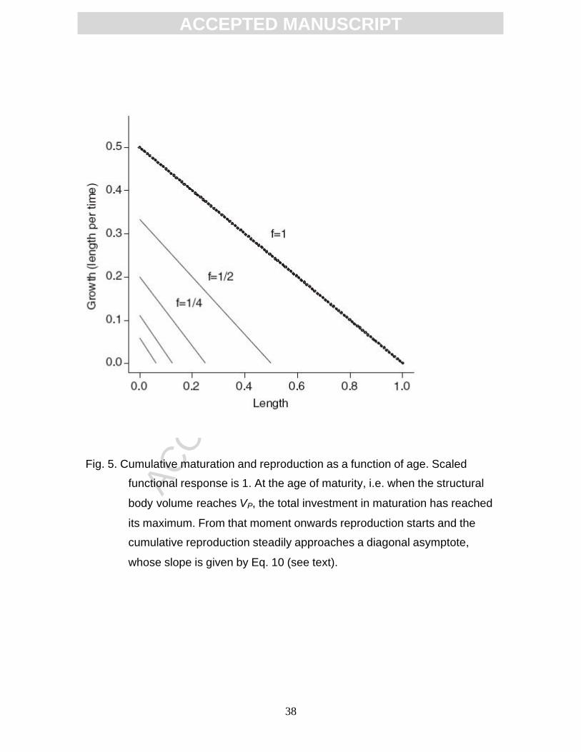
Fig. 5. Cumulative maturation and reproduction as a function of age. Scaled

functional response is 1. At the age of maturity, i.e. when the structural

body volume reaches VP, the total investment in maturation has reached

its maximum. From that moment onwards reproduction starts and the

cumulative reproduction steadily approaches a diagonal asymptote,

whose slope is given by Eq. 10 (see text).

ACC

EPTE

D M

ANU

SCR

IPT

ACCEPTED MANUSCRIPT

39

Fig. 6. The relation between body wet mass and shell length for the blue mussel

Mytilus edulis. The fitted curve is based on a weighted least-squares

procedure. The error variance clearly increases with length and the

weights were chosen proportional to shell length. Figure after Van Haren

and Kooijman (1993; fig. 1).

ACC

EPTE

D M

ANU

SCR

IPT

ACCEPTED MANUSCRIPT

40

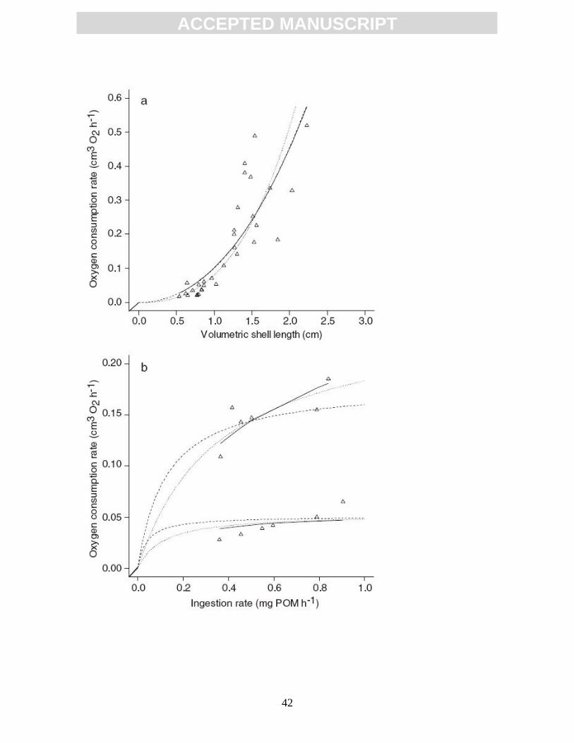
Fig. 7. Oxygen consumption rate as a function of (a) shell length and (b)

ingestion rate and shell length for the blue mussel Mytilus edulis. In

panel (b) squares indicate a shell length of 4.5 cm, circles a shell length

of 2.5 cm. Curves are given by Eq. 20. Solid lines refer to the parameter

estimates when the two datasets were used separately. Dotted and

dashed lines refer to the jointly estimated parameters, using different

weights. See also Table 3. Figure after Van Haren and Kooijman, (1993;

figs. 8 and 9).

ACC

EPTE

D M

ANU

SCR

IPT

ACCEPTED MANUSCRIPT

42

ACC

EPTE

D M

ANU

SCR

IPT

ACCEPTED MANUSCRIPT

43

Fig. 8. Shell length of the blue mussel Mytilus edulis in the Oosterschelde estuary

during 1985 and 1986. Figure after Van Haren and Kooijman (1993, figs.

14 and 15).

ACC

EPTE

D M

ANU

SCR

IPT

ACCEPTED MANUSCRIPT

44

TablesTable 1. The basic assumptions of the κ-rule DEB model.

1. An organism is characterised by a structural body and a reserve density (i.e.

amount of reserves per amount of structural body). The chemical composition

of both structural body and reserves is constant, which is called the

assumption of strong homeostasis.

2. Each organism starts its life as an embryo (which does not feed and does not

reproduce). When the embryo has reached a certain degree of maturation, it

changes into a juvenile (which feeds, but does not reproduce). Similarly, a

juvenile changes into an adult (which feeds and reproduces) when it exceeds

a given threshold value.

3. Ingestion is proportional to the surface area of the organism and depends

upon food density by a Holling type II functional response. Recall that

embryos do not feed.

4. A fixed fraction of the ingested food is assimilated and enters a storage pool,

which is characterised by the reserve density.

5. The regulation of the reserve density follows a first-order process.

6. A fixed fraction κ of the utilisation rate goes to somatic maintenance, heating

(for endotherms) and growth of the structural body (with a priority for

maintenance), and the rest goes to maturity maintenance and (for embryos

and juveniles) maturity or (for adults) reproduction.

7. Maintenance rate is proportional to structural volume and heating rate is

proportional to the surface area of the organism

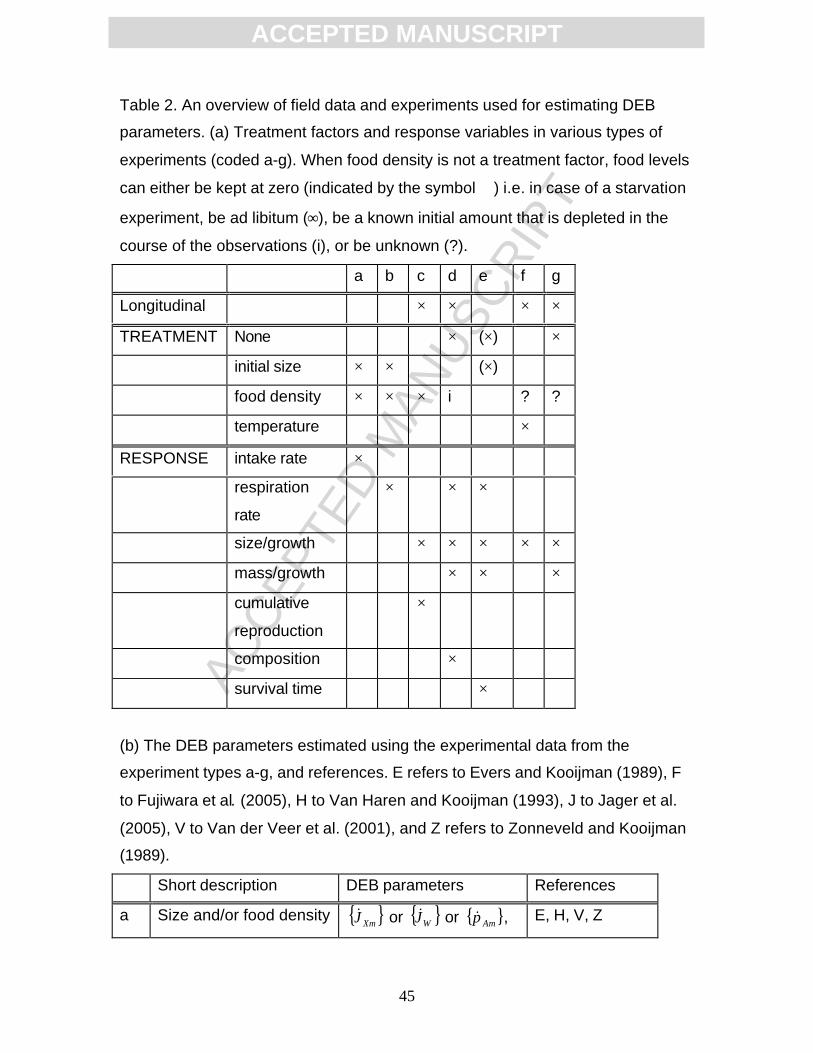
ACC

EPTE

D M

ANU

SCR

IPT

ACCEPTED MANUSCRIPT

45

Table 2. An overview of field data and experiments used for estimating DEB

parameters. (a) Treatment factors and response variables in various types of

experiments (coded a-g). When food density is not a treatment factor, food levels

can either be kept at zero (indicated by the symbol ∅) i.e. in case of a starvation

experiment, be ad libitum (∞), be a known initial amount that is depleted in the

course of the observations (i), or be unknown (?).

a b c d e f g

Longitudinal × × × ×

TREATMENT None × (×) ×

initial size × × (×)

food density × × × i ∅ ? ?

temperature ×

RESPONSE intake rate ×

respiration

rate

× × ×

size/growth × × × × ×

mass/growth × × ×

cumulative

reproduction

×

composition ×

survival time ×

(b) The DEB parameters estimated using the experimental data from the

experiment types a-g, and references. E refers to Evers and Kooijman (1989), F

to Fujiwara et al. (2005), H to Van Haren and Kooijman (1993), J to Jager et al.

(2005), V to Van der Veer et al. (2001), and Z refers to Zonneveld and Kooijman

(1989).

Short description DEB parameters References

a Size and/or food density { }XmJ& or { }WJ& or { }Amp& , E, H, V, Z

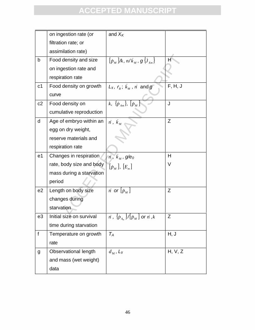
ACC

EPTE

D M

ANU

SCR

IPT

ACCEPTED MANUSCRIPT

46

on ingestion rate (or

filtration rate; or

assimilation rate)

and XK

b Food density and size

on ingestion rate and

respiration rate

[ ]Mp& /κ, ν/ Mk& , g { }XmJ& H

c1 Food density on growth

curve

L∞, Br& ; Mk& , ν& and g F, H, J

c2 Food density on

cumulative reproduction

κ, { }Amp& , [ ]Mp& J

d Age of embryo within an

egg on dry weight,

reserve materials and

respiration rate

ν& , Mk& Z

e1 Changes in respiration

rate, body size and body

mass during a starvation

period

ν& , Mk& , g/e0

[ ]Mp& , [ ]mE

H

V

e2 Length on body size

changes during

starvation

ν& or [ ]Mp& Z

e3 Initial size on survival

time during starvation

ν& , { }mAp& /[ ]Mp& or ν& ,κ Z

f Temperature on growth

rate

TA H, J

g Observational length

and mass (wet weight)

data

Μδ , L∞ H, V, Z

ACC

EPTE

D M

ANU

SCR

IPT

ACCEPTED MANUSCRIPT

47

Table 3. Estimates of DEB parameters for the blue mussel, based on Van Haren

and Kooijman (1993).

Data Original estimates My estimates

1 Length and wet

weight data

3Μ

δ = 0.03692 ± 7.59⋅10-5 3Μ

δ = 0.03692 ± 6.15⋅10-4

(using WLS with length

as weights)

2 Size on filtration

rate

{ }WJ& = 0.041 ± 0.000675

dm3 h-1 cm-2

{ }WJ& = 0.378 ± 0.00522

dm3 h-1 cm-2

After temperature

correction to 15 °C:

{ }WJ& = 0.499 dm3 h-1 cm-

2

3 Food density and

size on filtration

rate

{ }W mJ& = 0.83 ± 0.098 dm3

h-1 cm-2

XK = 76 106 ± 42 106 cells

dm-3

{ }W mJ& = 0.831 ± 0.101

dm3 h-1 cm-2

XK = 73.6 106 ± 41.7 106

cells dm-3

2&3

combined

{ }W mJ& = 0.831 ± 0.0837

dm3 h-1 cm-2

XK = 68.5 106 ± 27.2 106

cells dm-3

This gives:

{ }WJ& = 0.525 dm3 h-1 cm-

2

4 Size on oxygen

consumption rate

ν& / Mk& = 26.5 ± 14.8 mm ν& / Mk& = 7.67 ± 15.52 mm

5 Size and

ingestion rate on

oxygen

consumption rate

[ ] κη Mp& = 0.056 ± 0.025

cm3 O2 h-1 cm-3

ν& / Mk& = 5.3 ± 6.5 mm

[ ] κη Mp& = 0.072 ± 0.041

cm3 O2 h-1 cm-3

ν& / Mk& = 0.27 ± 0.54 mm

ACC

EPTE

D M

ANU

SCR

IPT

ACCEPTED MANUSCRIPT

48

g { }XmJ& = 0.16 ± 0.07 mg

POM cm-2 h-1

g { }XmJ& = 0.22 ± 0.13 mg

POM cm-2 h-1

4&5

combined

Equal weighing of 4 and

5:

[ ] κη Mp& = 0.0098 ±

0.0148 cm3 O2 h-1 cm-3

ν& / Mk& = 6.69 ± 10.71 mm

g { }XmJ& = 0.056 ± 0.159

mg POM cm-2 h-1

Non-equal weighing of 4

and 5:

[ ] κη Mp& = 0.0511 ±

0.0201 cm3 O2 h-1 cm-3

ν& / Mk& =0.672 ± 0.543

mm

g { }XmJ& = 0.161 ± 0.0664

mg POM cm-2 h-1

ACC

EPTE

D M

ANU

SCR

IPT

ACCEPTED MANUSCRIPT

49

Appendix 1. A list of important DEB parameters

DEB uses a notation that is helpful in a quick interpretation of the equations. All

rates have dots, which indicate that they contain the dimension ‘per time’. All

variables that are expressed per unit volume are given between square brackets.

All variables that are expressed per unit surface area are given between braces.

Notation from Kooijman (2000) is used. The earlier papers and books (Kooijman,

1986a, b, 1993) used slightly different notations, shown in the column Previous

symbols.

Symbol Dimensio

n

Interpretation Previous

symbols

[ ]E eL-3 Energy density

L L Body length

V L3 Structural body volume

F - Scaled functional response

T T Temperature

X #l-2 or #l-3 Food density in the environment

Symbol Dimensio

n

Interpretation Previous

symbols

[ ]GE eL-3 Volume-specific costs of growth η,[ ]G

[ ]mE eL-3 Maximum energy density [ ]mS ,[ ]mE

{ }XmJ& #L-2t-1 Surface-area-specific maximum

ingestion rate

[ ]mI& ,{ }mI&

{ }Amp& eL-2t-1 Surface-area-specific maximum

assimilation rate

[ ]mA& , { }mA&

[ ]Mp& eL-2t-1 Volume-specific maintenance rate &ς ,[ ]&M

{ }Tp& eL-2t-1 Surface-area-specific heating rate

TA T Arrhenius temperature

ACC

EPTE

D M

ANU

SCR

IPT

ACCEPTED MANUSCRIPT

50

XK #l-2 or #l-3 Saturation coefficient K

Μδ - Shape (morph) coefficient

κ - Fraction of utilisation rate spent on

maintenance plus growth

Symbol Dimensio

n

Interpretation Previous

symbols

g -Energy investment ratio

[ ][ ]m

G

EE

κ

Mk& t-1Maintenance rate coefficient

[ ][ ]G

M

Ep& m&

ν& Lt-1Energy conductance

{ }[ ]M

Am

Ep&

mL L Maximum volumetric length

{ } { }[ ]M

TAm

ppp

&&& −κ

∞L L Ultimate volumetric length

{ } { }[ ]M

TAm

pppf

&&& −κ

Br& t-1 Von Bertalanffy growth coefficient

[ ][ ] [ ]GM

M

EEfp

+κ&

31

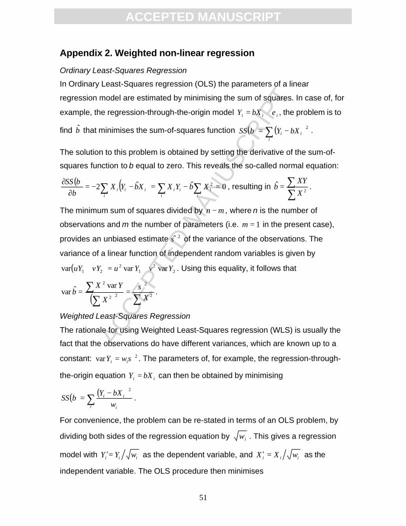
ACC

EPTE

D M

ANU

SCR

IPT

ACCEPTED MANUSCRIPT

51

Appendix 2. Weighted non-linear regression

Ordinary Least-Squares Regression

In Ordinary Least-Squares regression (OLS) the parameters of a linear

regression model are estimated by minimising the sum of squares. In case of, for

example, the regression-through-the-origin model iii bXY ε+= , the problem is to

find b that minimises the sum-of-squares function ( ) ( )∑ −=i

ii bXYbSS 2 .

The solution to this problem is obtained by setting the derivative of the sum-of-

squares function to b equal to zero. This reveals the so-called normal equation:

( ) ( ) 0ˆˆ2 2 =−=−−=∂

∂ ∑∑∑i

ii

iii

iii XbYXXbYXbbSS

, resulting in ∑∑=

2ˆ

X

XYb .

The minimum sum of squares divided by mn − , where n is the number of

observations and m the number of parameters (i.e. 1=m in the present case),

provides an unbiased estimate 2σ of the variance of the observations. The

variance of a linear function of independent random variables is given by

( ) 22

12

21 varvarvar YvYuvYuY +=+ . Using this equality, it follows that

( ) ∑∑∑ == 2

2

22

2 varˆvarXX

YXb

σ.

Weighted Least-Squares Regression

The rationale for using Weighted Least-Squares regression (WLS) is usually the

fact that the observations do have different variances, which are known up to a

constant: 2var σii wY = . The parameters of, for example, the regression-through-

the-origin equation ii bXY = can then be obtained by minimising

( ) ( )∑ −=

i i

ii

wbXY

bSS2

.

For convenience, the problem can be re-stated in terms of an OLS problem, by

dividing both sides of the regression equation by iw . This gives a regression

model with iii wYY =′ as the dependent variable, and iii wXX =′ as the

independent variable. The OLS procedure then minimises

ACC

EPTE

D M

ANU

SCR

IPT

ACCEPTED MANUSCRIPT

52

( ) ( ) ( )∑∑∑

−=

−=′−′=

i i

ii

i i

i

i

i

iii w

bXY

w

Xb

w

YXbYbSS

22

2 ,

and is thus equivalent to WLS.

Non-linear Least-Squares Regression

The problem with non-linear equations is that the normal equations cannot be

solved analytically. For example, in case of the model

ibii aXY ε+= , the normal equations are given by

( ) ( ) 0ˆ2, ˆˆ

=−−=∂

∂ ∑i

bii

bi XaYX

abaSS

( ) ( ) ( ) 0ˆˆlog2, ˆˆ

=−−=∂

∂ ∑i

bii

bii XaYXaX

bbaSS

,

which illustrates their intractable nature, i.e. the equations cannot easily be

solved for a and b . Numerical iterative methods are required to find the least-

squares solution. See, for example, Seber and Wild (1989) for an introduction to

non-linear regression.