Acceptance Sampling McGraw-Hill/Irwin Copyright © 2012 by The McGraw-Hill Companies, Inc. All rights reserved

Acceptance Sampling

McGraw-Hill/Irwin Copyright © 2012 by The McGraw-Hill Companies, Inc. All rights reserved.

You should be able to:1. Explain the purpose of acceptance sampling2. Contrast acceptance sampling and process

control3. Compare and contrast single- and multiple-

sampling plans4. Determine the average outgoing quality of

inspected lots

Instructor Slides 10S-2

Acceptance samplingA form of inspection applied to lots or batches

of items before or after a process, to judge conformance with predetermined standards

May be applied to both attribute and variable inspection


The purpose of acceptance sampling is to decide whether a lot satisfies predetermined standardsLots that satisfy these standards are passed or

acceptedRejected lots may be subjected to 100 percent

inspectionIn the case of purchased goods, they may be

returned for credit or replacement


Acceptance sampling is most useful when at least one of the following conditions exists:1. A large number of items must be processed in a short

time2. The cost consequences of passing defectives are low3. Destruction testing is required4. Fatigue or boredom caused by inspecting large

numbers of items leads to inspection errors


Sampling plans:Plans that specify lot size, sample size, number

of samples, and acceptance/rejection criteriaSingle-sampling planDouble-sampling planMultiple-sampling plan


Single-sampling planOne random sample is drawn from each lotEvery item in the sample is inspected and

classified as “good” or “defective”If any sample contains more than a specified

number of defectives, c, the lot is rejected


Double-Sampling Plan Allows the opportunity to take a second sample if the results

of the initial sample are inconclusiveTwo values are specified for the number of defective items

A lower level, c1

An upper level, c2 If the number of defectives in the first sample is

≤ c1 the lot is accepted and sampling is terminated > c2 the lot is rejected and sampling is terminated Between c1 and c2 a second sample is collected

The number of defectives in both samples is compared to a third value, c3 If the combined number of defectives does not exceed this

value, the lot is accepted; otherwise, it is rejected


Multiple-sampling plan Similar to a double-sampling plan except more than two

samples may be required A sampling plan will specify each sample size and two limits

for each sampleThe limit values increase with the number of samples If, for any sample, the cumulative number of defectives

found exceeds the upper limit specified, the lot is rejected If for any sample the cumulative number of defectives

found is less than or equal to the lower limit, the lot is accepted.

If the number of defectives found is between the two limits, another sample is taken

The process continues until the lot is accepted or rejected


Sampling plan choice is dictated by cost and time required for inspectionTwo primary considerations:

Number of samples neededTotal number of observations required


Single-sampling plan requires only one sample; however, the sample size is large compared to the total number of observations taken under double- or multiple-sampling plansSingle-sampling plans preferred when the cost of

collecting a sample is high relative to the cost of analyzing the observations

When cost of analyzing observations is high (e.g., destructive testing), double- or multiple-sampling plans are more desirable


An important sampling plan characteristic is how it discriminates between high and low quality

OC curves describe a sampling plan’s ability to discriminate OC curve

Probability curve that shows the probabilities of accepting lots with various fractions defective


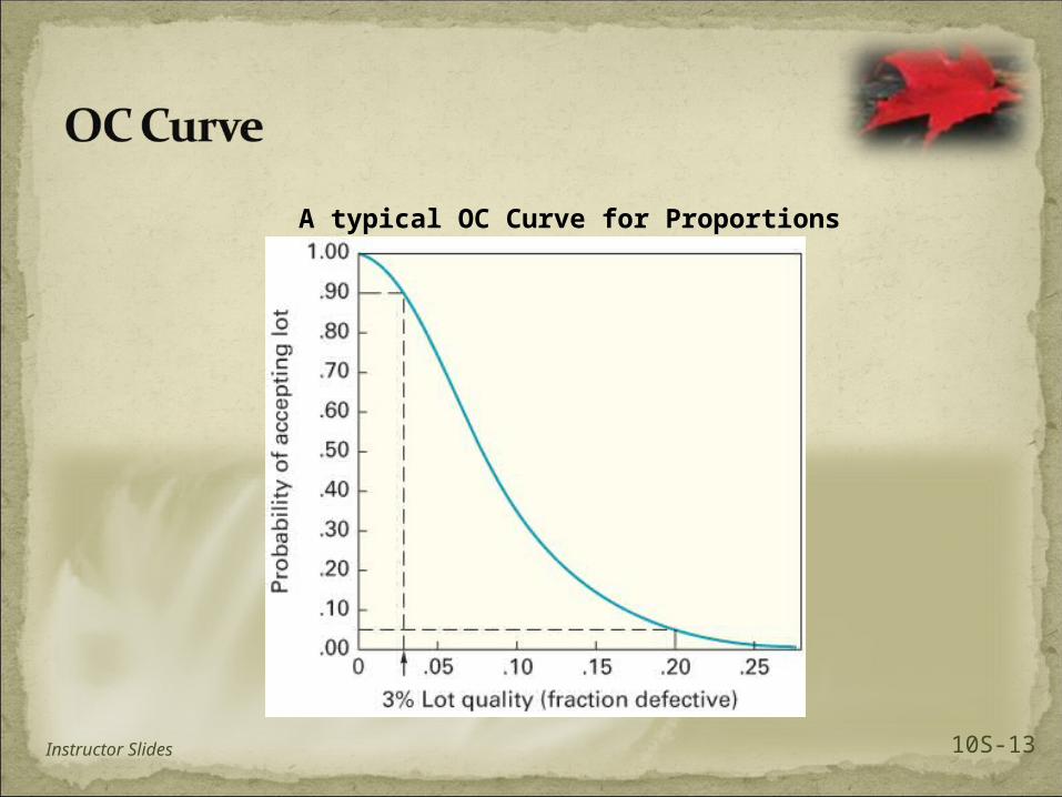
A typical OC Curve for Proportions


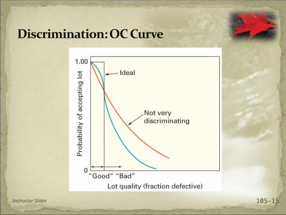
No sampling plan perfectly discriminates between good and bad quality

The degree to which a sampling plan discriminates is a function of the graph’s OC curve Steeper OC curves are more discriminating



To perfectly discriminate, theoretically, between “good” and “bad” quality would require 100% inspection.

100% inspection is impracticalCostly and time-consumingDestructive testing


Given the impracticality of 100% inspection, buyers are willing to live with a small number of defectives if the cost of doing so is lowUsually, in the range of 1% - 2% defective


Acceptable quality Level (AQL)The percentage level of defects at which

consumers are willing to accept lots as “good”Lot tolerance percent defective (LTPD)

The upper limit on the percentage of defects that a consumer is willing to accept


Customers want quality equal to or better than the AQL, and are willing to accept some lots with quality as poor as the LTPD, but they prefer not to accept any lots with a defective percentage that exceeds the LTPD


Consumer’s risk, βThe probability that a lot containing defects

exceeding LTPD will be acceptedManufacturer’s risk, α

The probability that a lot containing the acceptable quality level will be rejected


Many sampling plans are developed to have a Producer’s risk of 5 percent Consumer’s risk of 10 percent

Standard references are widely available to obtain sample sizes and acceptance criteria for sampling plans Government MIL-STD tables


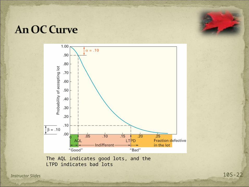
The AQL indicates good lots, and the LTPD indicates bad lots


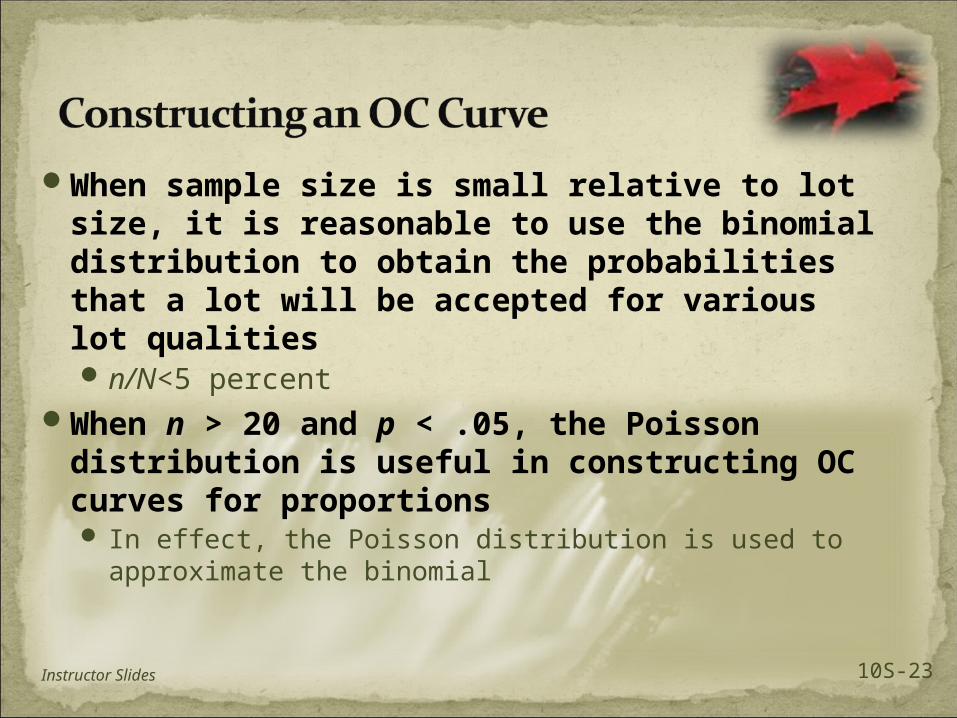
When sample size is small relative to lot size, it is reasonable to use the binomial distribution to obtain the probabilities that a lot will be accepted for various lot qualitiesn/N<5 percent

When n > 20 and p < .05, the Poisson distribution is useful in constructing OC curves for proportions In effect, the Poisson distribution is used to approximate

the binomial


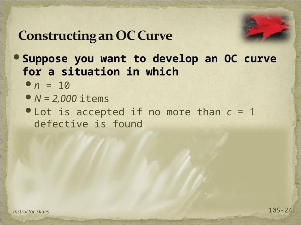
Suppose you want to develop an OC curve for a situation in whichn = 10N = 2,000 itemsLot is accepted if no more than c = 1 defective

is found


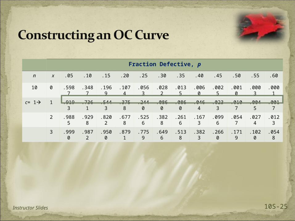
Fraction Defective, p

n x .05 .10 .15 .20 .25 .30 .35 .40 .45 .50 .55 .60

10 0 .5987

.3487

.1969

.1074

.0563

.0282

.0135

.0060

.0025

.0010

.0003

.0001

c= 1 1 .9193

.7361

.5443

.3758

.2440

.0860

.0860

.0464

.0233

.0107

.0045

.0017

2 .9885

.9298

.8202

.6778

.5256

.3828

.2616

.1673

.0996

.0547

.0274

.0123

3 .9990

.9872

.9500

.8791

.7759

.6496

.5138

.3823

.2660

.1719

.1020

.0548


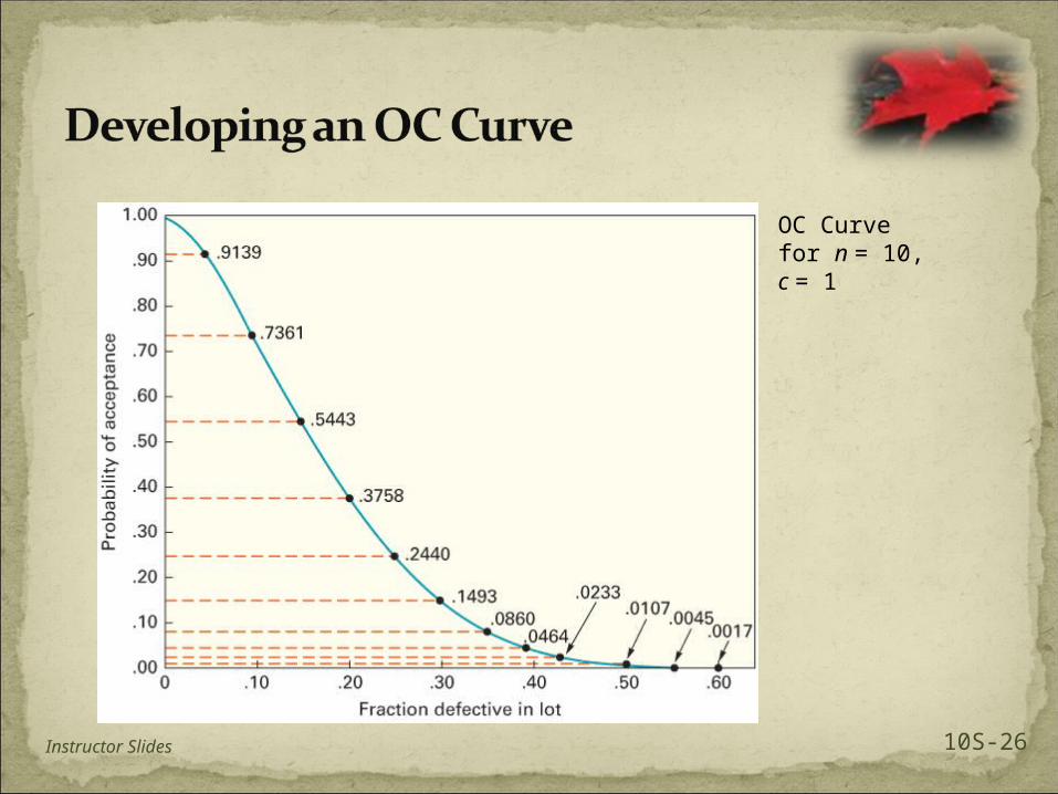
OC Curve for n = 10, c = 1


An interesting feature of acceptance sampling is that the level of inspection automatically adjusts to the quality of the lots being inspected, assuming rejected lots are subjected to 100 percent inspectionGood lots have a high probability and bad lots

a low probability of being accepted.If the lots inspected are mostly good, few will end

up going through 100 percent inspection.The poorer the quality of the lots, the greater the

number of lots that will come under close scrutiny


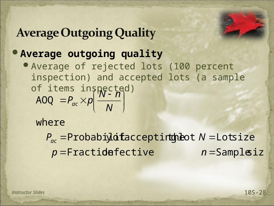
Average outgoing qualityAverage of rejected lots (100 percent

inspection) and accepted lots (a sample of items inspected)

size Sample defectiveFraction

sizeLot lot theaccepting ofy Probabilit

where

AOQ

np

NP

N

nNpP

ac

ac


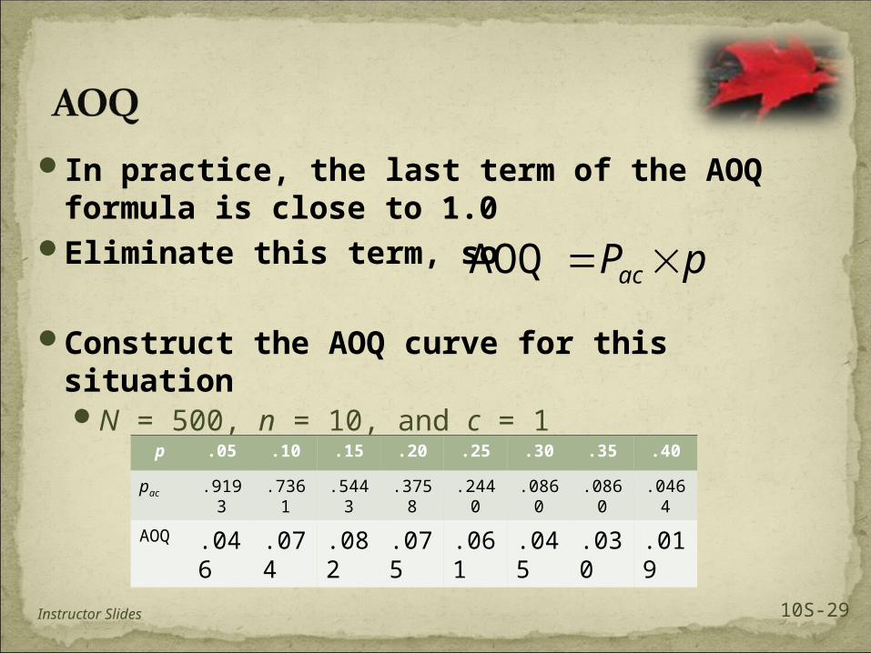
In practice, the last term of the AOQ formula is close to 1.0

Eliminate this term, so

Construct the AOQ curve for this situationN = 500, n = 10, and c = 1

pPac AOQ

p .05 .10 .15 .20 .25 .30 .35 .40

pac .9193

.7361

.5443

.3758

.2440

.0860

.0860

.0464

AOQ .046

.074

.082

.075

.061

.045

.030

.019


0

0.02

0.04

0.06

0.08

0.1

0 0.1 0.2 0.3 0.4 0.5

AO

Q

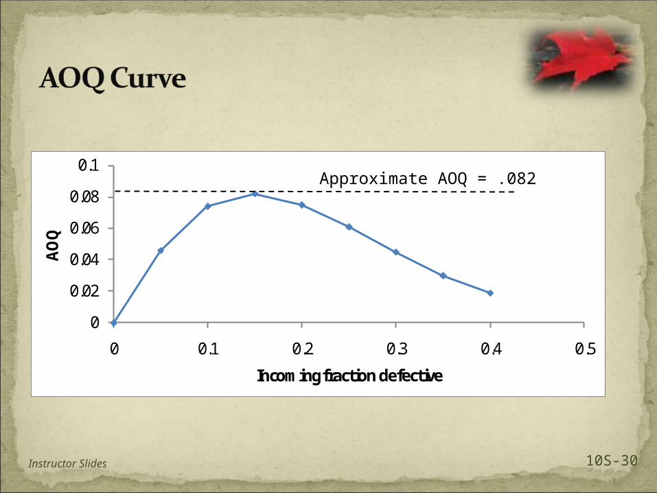
Incoming fraction defective

Approximate AOQ = .082


A manager can determine the worst possible outgoing quality

The manager can determine the amount of inspection that will be needed by obtaining an estimate of the incoming quality

Information can be used to establish the relationship between inspection cost and the incoming fraction defective Underscores the benefit of process improvement over weeding

out defectives via inspection


Documents

Acceptance Sampling McGraw-Hill/Irwin Copyright © 2012 by The McGraw-Hill Companies, Inc. All rights reserved