Accelerator Physics : Real Life or

some stuff you can hardly find in accelerator physics textbooks

Yuri Saveliev ASTeC, STFC, CI

CI Accelerator Physics School, November 2013 1

What is this lecture about ….

“Why practically all books on accelerator physics written by theoreticians? And virtually all of them are about theory?”

“Because experimentalists do not have time to write books … “ Mike Poole, former ASTeC director

This lecture: • is not a “textbook”, instead it gives just a number of examples when things in

“real life” are not quite the same as “on paper” • hopes to give you some practical advices on how “to do” or “not to do” things

in the control room of the accelerator and how to interpret experimental data you gathered

• will perhaps, explain why experimentalists do not have time to write books … • is based on (mostly) experiences we gathered from commissioning ALICE and

from experiments with ALICE electron beam

2

ALICE a very brief overview

3

EMMA

superconducting linac DC gun

photoinjector laser Free Electron

Laser

superconducting booster

The ALICE Facility @ Daresbury Laboratory

Accelerators and Lasers In Combined Experiments

An accelerator R&D facility based on a superconducting energy recovery linac

4

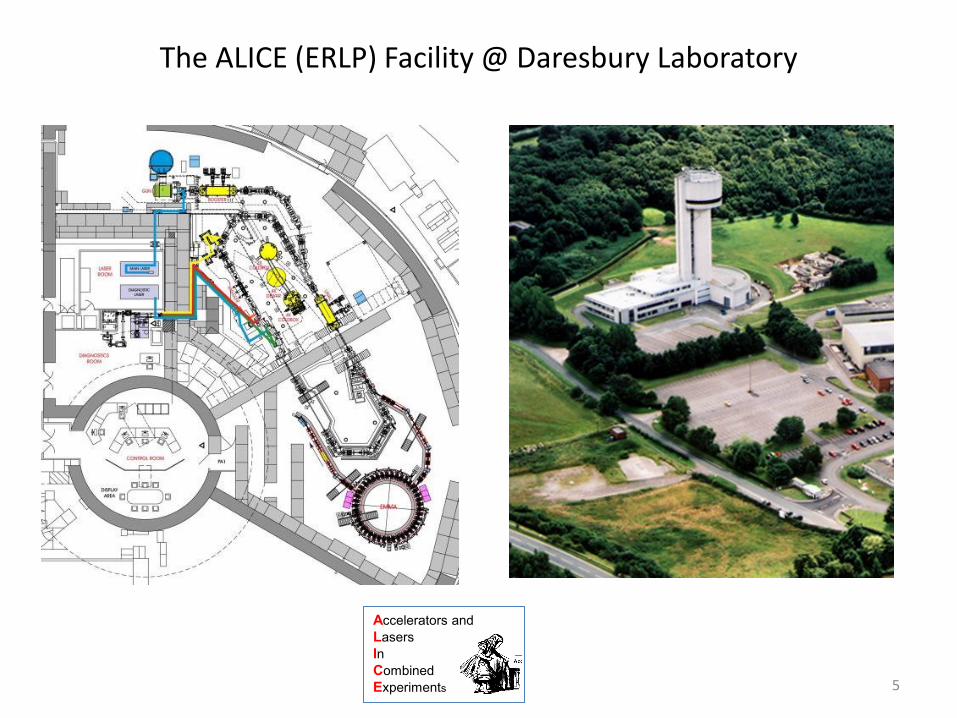
The ALICE (ERLP) Facility @ Daresbury Laboratory

Tower or lab

picture

Accelerators and

Lasers

In

Combined

Experiments 5

ALICE schematic and main components

Photoinjector laser (28ps) Photogun (325keV) RF buncher (1.3GHz) RF SC booster (1.3GHz; 6.5MeV) Injector beamline main linac (1.3GHz; 26.0MeV) 1st arc Compression chicane (<1ps bunches) THz source undulator (IR FEL) 2nd arc Main linac (energy recovery; 26.0MeV to 6.5MeV) main beam dump

Systems : cryogenic , vacuum, magnetic , RF, diagnostics, controls … 6

ALICE : HV DC Photogun

ALICE : Superconductive linac

7

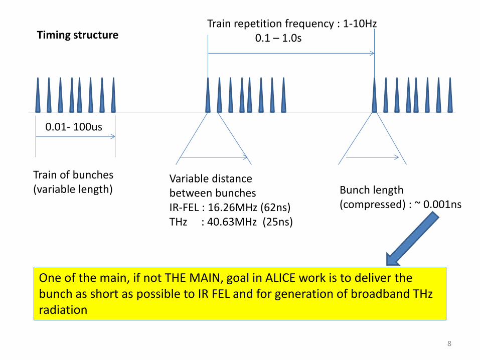
Timing structure

0.01- 100us

Train of bunches (variable length)

Variable distance between bunches IR-FEL : 16.26MHz (62ns) THz : 40.63MHz (25ns)

Bunch length (compressed) : ~ 0.001ns

Train repetition frequency : 1-10Hz 0.1 – 1.0s

One of the main, if not THE MAIN, goal in ALICE work is to deliver the bunch as short as possible to IR FEL and for generation of broadband THz radiation

8

Nothing is perfect in real life

Neither the machine nor the beam nor the model nor the guy who turns the knobs …

9

Searching for Holy Grail : validating the machine model

No model can fully reflect and take into account all the complexity of physics governing the beam behaviour in an accelerator No machine is built absolutely perfectly corresponding to the model

Need to adjust and validate the model by tweaking it

Why ? We need the model to be as close to “real life” as possible for e.g. (i) we need to reliably know what is happening with the beam between diagnostic places where we can see the beam (ii) we always need to tune and retune the machine for different setups

How? … by making measurements in the first instance !

10

“If you see a tiger in a cage labelled “Lion” – do not believe your eyes” Koz’ma Prutkov

Dilemma encountered in experimental accelerator physics well too often !

Just one example …

beam

BPM Quad Screen

Beam Position Monitor (BPM) says : beam centred ! Quad says : No!, I still steer the beam downstream !

• BPM channels not equalised ? (Hence the beam not really centred …) • BPM or quad or both misaligned ? (Well, nothing is perfect …) • Beam actually enters BPM with large angle wrt axis ? (Oh, that has to be checked !)

11

Gaussian beams ? … forget it ! … in many cases, at least

Jlab’s “humming bird” beam image

12

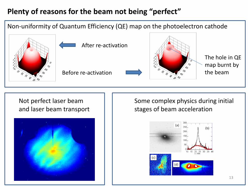
Before re-activation

After re-activation

Plenty of reasons for the beam not being “perfect”

Non-uniformity of Quantum Efficiency (QE) map on the photoelectron cathode

The hole in QE map burnt by the beam

Not perfect laser beam and laser beam transport

Some complex physics during initial stages of beam acceleration

13

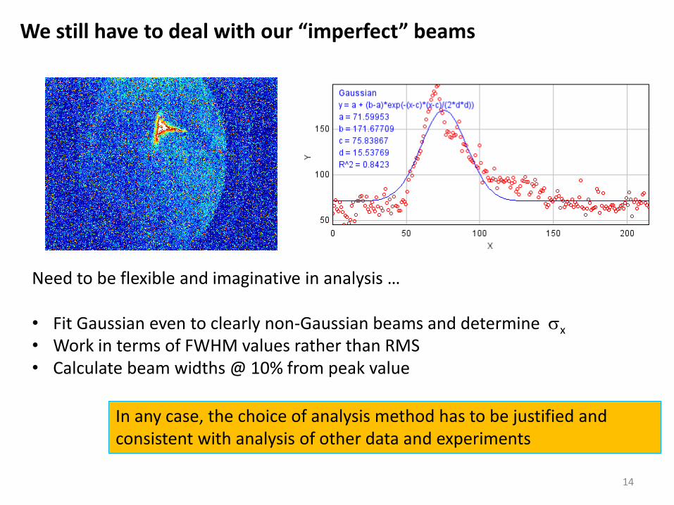
We still have to deal with our “imperfect” beams

Need to be flexible and imaginative in analysis … • Fit Gaussian even to clearly non-Gaussian beams and determine sx • Work in terms of FWHM values rather than RMS • Calculate beam widths @ 10% from peak value

In any case, the choice of analysis method has to be justified and consistent with analysis of other data and experiments

14

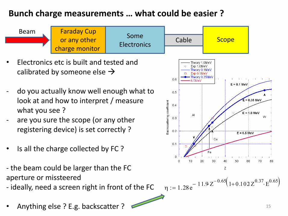
Bunch charge measurements … what could be easier ?

Faraday Cup or any other

charge monitor Cable

Some Electronics

Scope Beam

• Electronics etc is built and tested and calibrated by someone else

- do you actually know well enough what to

look at and how to interpret / measure what you see ?

- are you sure the scope (or any other registering device) is set correctly ?

• Is all the charge collected by FC ?

- the beam could be larger than the FC aperture or missteered - ideally, need a screen right in front of the FC

• Anything else ? E.g. backscatter ?

1.28e11.9 Z

0.65 1 0.102 Z

0.37 E

0.65

15

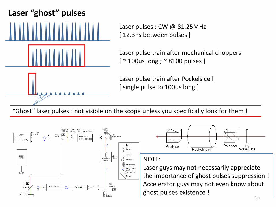
Laser “ghost” pulses

Laser pulses : CW @ 81.25MHz [ 12.3ns between pulses ]

“Ghost” laser pulses : not visible on the scope unless you specifically look for them !

Laser pulse train after mechanical choppers [ ~ 100us long ; ~ 8100 pulses ]

Laser pulse train after Pockels cell [ single pulse to 100us long ]

NOTE: Laser guys may not necessarily appreciate the importance of ghost pulses suppression ! Accelerator guys may not even know about ghost pulses existence !

16

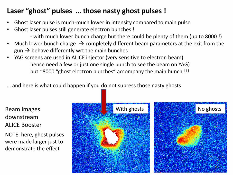
No ghosts With ghosts Beam images downstream ALICE Booster

• Ghost laser pulse is much-much lower in intensity compared to main pulse • Ghost laser pulses still generate electron bunches ! - with much lower bunch charge but there could be plenty of them (up to 8000 !) • Much lower bunch charge completely different beam parameters at the exit from the

gun behave differently wrt the main bunches • YAG screens are used in ALICE injector (very sensitive to electron beam) hence need a few or just one single bunch to see the beam on YAG) but ~8000 “ghost electron bunches” accompany the main bunch !!! … and here is what could happen if you do not supress those nasty ghosts

Laser “ghost” pulses … those nasty ghost pulses !

NOTE: here, ghost pulses were made larger just to demonstrate the effect

17

Twiss parameters measurements

This is one of the important methods for accelerator model development and validation There are many other methods to investigate the beam optics and the machine lattice but we will not talk about anything else here

18

Back to model validation … need Twiss parameters measured

Quadrupole scans

Simplest configuration : {quad drift screen} (large L can use thin lens approximation) Word of caution : if there are any other quads between the scanning quad and the screen, they MUST be thoroughly degaussed, just switching them off is not enough (remnant fields !)

• Vary the quad strength • Collect images and measure RMS beam sizes • Plot beam size squared v quad’s (kl) values • Fit parabola and find its A,B,C coefficients • Calculate Twiss (emittance, beta, alpha)

19

Q-scans : Fitting parabola to experimental data

Built-in fitting programmes use polynomial fit: 𝜎2 = 𝑎(𝑘𝑙)2+𝑏 𝑘𝑙 + 𝑐 eventual formulae for Twiss calculations are bulky and not intuitive

Much better this way : 𝜎2 = 𝐴(𝑘𝑙 − 𝐵)2+𝐶

A controls “steepness” of

parabola wings

B = (kl) value at which

parabola (and beam size !) reaches its minimum

C = minimal value

of the beam size

휀 =𝐴𝐶

𝑆122

𝛽 =𝐴

𝐶

𝛼 =𝐴

𝐶 −𝐵 +

𝑆11

𝑆12

Twiss parameters from parabola fit

• S – matrix from quad exit to screen • Thin lens approximation for a quad • Emittance - geometric !

In simple case of quad/drift = L /screen: 𝑆11 = 1; 𝑆12 = 𝐿

20

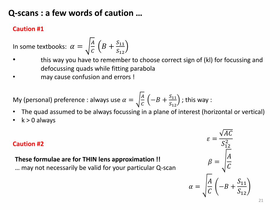
Q-scans : a few words of caution …

Caution #1

In some textbooks: 𝛼 =𝐴

𝐶 𝐵 +

𝑆11

𝑆12

• this way you have to remember to choose correct sign of (kl) for focussing and defocussing quads while fitting parabola

• may cause confusion and errors !

My (personal) preference : always use 𝛼 =𝐴

𝐶 −𝐵 +

𝑆11

𝑆12 ; this way :

• The quad assumed to be always focussing in a plane of interest (horizontal or vertical) • k > 0 always

21

Caution #2 휀 =

𝐴𝐶

𝑆122

𝛽 =𝐴

𝐶

𝛼 =𝐴

𝐶 −𝐵 +

𝑆11

𝑆12

These formulae are for THIN lens approximation !! … may not necessarily be valid for your particular Q-scan

0

0.05

0.1

0.15

0.2

0.25

0.3

0.35

0.4

1 1.2 1.4 1.6 1.8 2 2.2 2.4 2.6

sigma-X^2fit

sig

ma

-X^2

kl (Q3)

0

1

2

3

4

5

6

0 1 2 3 4 5 6

sigma-X^2fit

sig

ma

-X^2

kl (Q3)

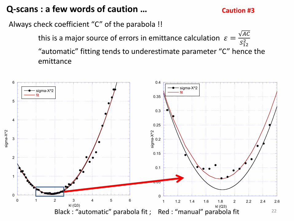
Q-scans : a few words of caution … Caution #3

Always check coefficient “C” of the parabola !!

this is a major source of errors in emittance calculation 휀 =𝐴𝐶

𝑆122

“automatic” fitting tends to underestimate parameter “C” hence the emittance

Black : “automatic” parabola fit ; Red : “manual” parabola fit 22

In experimental physics, it’s always advisable to cross-check measurements by using different methods and techniques ….

23

e.g. we can measure the beam emittance by several different methods …

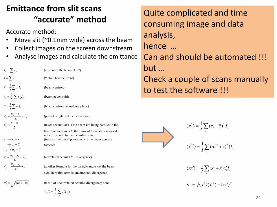
Emittance from slit scans “accurate” method Accurate method: • Move slit (~0.1mm wide) across the beam • Collect images on the screen downstream • Analyse images and calculate the emittance

j

iji II (current of the beamlet “i”)

i

iII (“total” beam current)

i

ii IxI

x1

(beam centroid)

j

ijij

i

i IuI

u1

(beamlet centroid)

i

ii IuI

u1

(beam centroid at analysis plane)

0xL

xux

iij

ij

(particle angle wrt the beam axis)

L

xux

0 (takes account of (1) the beam not being parallel to the

beamline axis and (2) the zeros of translation stages do

not correspond to the beamline axis)

xxx ii (transformations if positions wrt the beam axis are

uuu ii needed)

uuu ijij

0xL

xux ii

i

(correlated beamlet “i” divergence)

i

iij

ij xL

uux

(another formula for the particle angle wrt the beam

axis; here first term is uncorrelated divergence)

221iii uu

Ls (RMS of uncorrelated beamlet divergence; here

j

ijij

i

i IuI

u 22 1)

i

ii IxxI

x 22 )(1

i

iii IxI

x )(1 222 s

i

iii IxxxI

xx )(1

222 xxxxx

Quite complicated and time consuming image and data analysis, hence … Can and should be automated !!! but … Check a couple of scans manually to test the software !!!

24

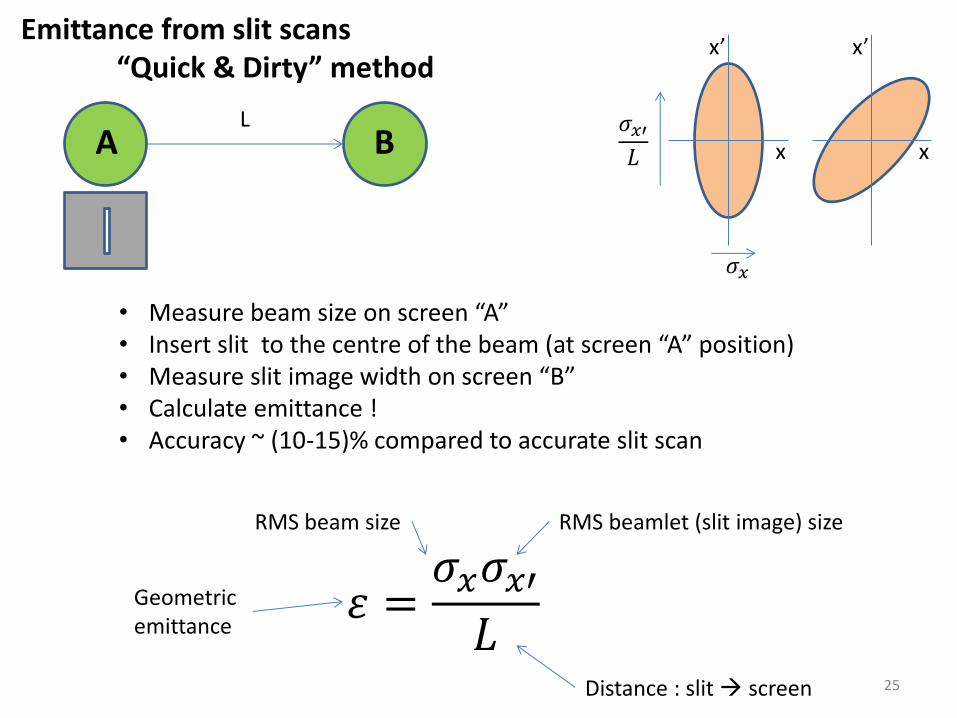
Emittance from slit scans “Quick & Dirty” method

휀 =𝜎𝑥𝜎𝑥′

𝐿 Geometric

emittance

RMS beam size RMS beamlet (slit image) size

Distance : slit screen

x’

x

x’

x

𝜎𝑥

𝜎𝑥′

𝐿

L

• Measure beam size on screen “A” • Insert slit to the centre of the beam (at screen “A” position) • Measure slit image width on screen “B” • Calculate emittance ! • Accuracy ~ (10-15)% compared to accurate slit scan

A B

25

Do not forget about “small print”

Plenty of things that affect what we see and measure …

26

YAG and OTR screens

YAG (Yttrium Aluminium Garnet) • Nice near mirror like finish • Often metal film coated • Large light output • Used at lower (<10MeV) beam energies

OTR (Optical Transition Radiation) • In principle, any material with dielectric

constant >1 • If foil, can get “wrinkles” • Low light output (<5% of YAG) • Light output depends on beam energy • Used at higher beam energies

27

Protons

o

Normal Incidence

Protons

o

Oblique Incidence

Beam energy = 12MeV ; both screens are next to each other Cameras: straight through for YAG; at 90deg for OTR

YAG screens at low beam energies

If The beam energy is low (say, < 20MeV) You trying to measure very small beam sizes ( < 1mm) Then Keep in mind some potential artefacts to be introduced

YAG OTR (foil)

Electron scattering leads to enlargement of the beam image on YAG screen

28

0

0.05

0.1

0.15

0.2

0.25

0.3

0.35

0 1 2 3 4 5 6 7 8

RMS beam size v train length

#1589 (INJ-3 image of INJ-2 slit)

Xrm

s,

mm

T, us

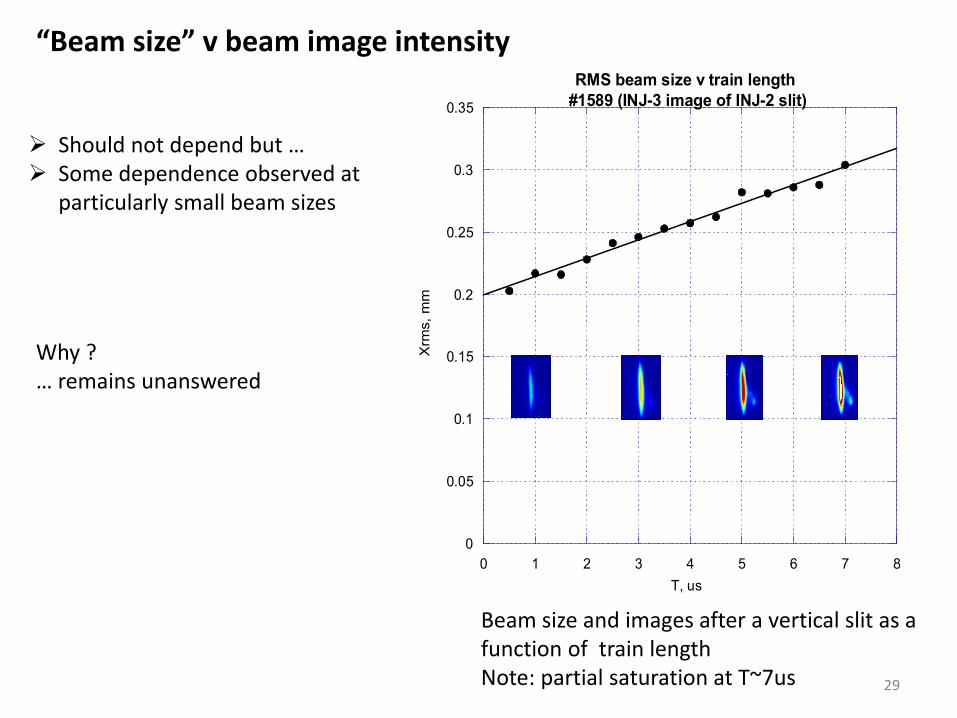
“Beam size” v beam image intensity

Should not depend but … Some dependence observed at

particularly small beam sizes

Beam size and images after a vertical slit as a function of train length Note: partial saturation at T~7us 29

Why ? … remains unanswered

T=10us

T=50us

EMMA setup (#3143; AR1-1)

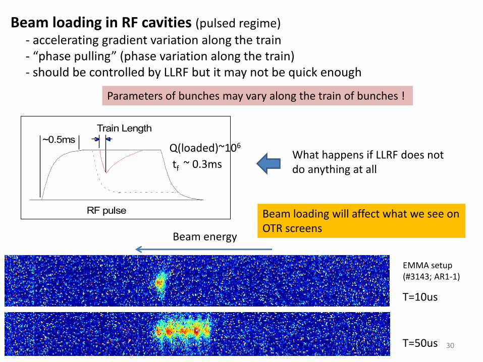
Beam loading in RF cavities (pulsed regime)

- accelerating gradient variation along the train - “phase pulling” (phase variation along the train) - should be controlled by LLRF but it may not be quick enough

Parameters of bunches may vary along the train of bunches !

~0.5msTrain Length

RF pulse

Q(loaded)~106

tf ~ 0.3ms What happens if LLRF does not do anything at all

Beam energy

Beam loading will affect what we see on OTR screens

30

Screen calibration factors

0.054

0.056

0.058

0.06

0.062

0.064

0.066

0.068

0.07

0 100 200 300 400 500 600

ST1-3 screen calibration (H) #2634

mm/pix

y = 0.048159 + 3.8003e-5x R= 0.98028

mm

/pix

x,pix

ST1-3 screen and calibration factor

Screen Calibration factor : mm/pixel

With larger screens positioned at 45deg to camera and /or

Cameras positioned close to the screen :

Calibration factor is NOT constant across the screen !

Graticules, markings, or just screen frames are used for calibration

Errors or mistakes in calibrations = waste of time Better be “paranoid” about validity of older calibrations

• “Human” errors • Zoomed cameras (and no markings) • Non-constant calibration factors across the screen

31

32

Beam energy & energy spread measurements

(small area of experimental physics but with many pitfalls)

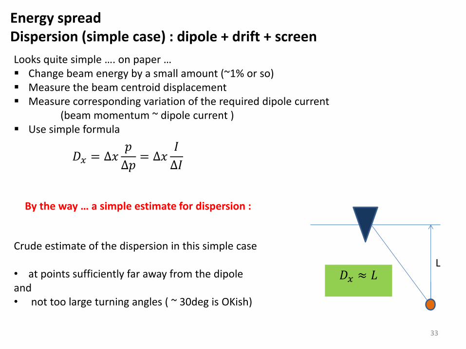
Energy spread Dispersion (simple case) : dipole + drift + screen

𝐷𝑥 = ∆𝑥𝑝

∆𝑝= ∆𝑥

𝐼

∆𝐼

Looks quite simple …. on paper … Change beam energy by a small amount (~1% or so) Measure the beam centroid displacement Measure corresponding variation of the required dipole current (beam momentum ~ dipole current ) Use simple formula

𝐷𝑥 ≈ 𝐿 L

Crude estimate of the dispersion in this simple case • at points sufficiently far away from the dipole and • not too large turning angles ( ~ 30deg is OKish)

33

By the way … a simple estimate for dispersion :

0

0.2

0.4

0.6

0.8

1

1.2

1.4

2.8 3 3.2 3.4 3.6 3.8 4 4.2

Dis

pe

rsio

n,

m

I0

6.5MeV

Q-05 not degaussed

0

0.5

1

1.5

5.2 5.4 5.6 5.8 6 6.2 6.4 6.6

Dx,m (from I)

y = 0.8283 + 0.042081x R= 0.14566

Dx,m

(fr

om

I)

Eb, MeV

Dispersion on INJ-5 (from current difference) #2897

Q-05 degaussed

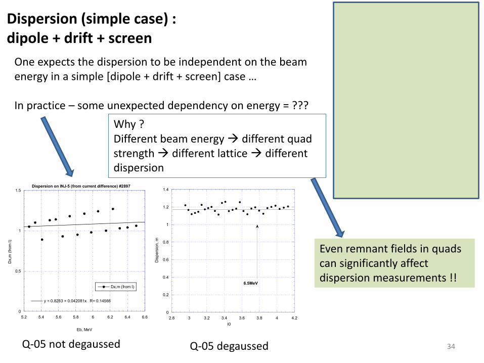
Dispersion (simple case) : dipole + drift + screen

ALICE injector energy Spectrometer Q-05 & DIP-02 switched off

One expects the dispersion to be independent on the beam energy in a simple [dipole + drift + screen] case … In practice – some unexpected dependency on energy = ???

Why ? Different beam energy different quad strength different lattice different dispersion

Even remnant fields in quads can significantly affect dispersion measurements !!

34

Dispersion : second (and higher) order effects

20

25

30

35

40

-4 -3 -2 -1 0 1 2 3 4

X,mmY,mm

be

am

po

sitio

n,m

m

dE/E

Y = M0 + M1*x + ... M8*x8 + M9*x

9

38.95M0

-0.43995M1

-0.3409M2

0.071861M3

0.99851RY = M0 + M1*x + ... M8*x

8 + M9*x

9

23.058M0

-0.068924M1

0.044878M2

0.99426R

Dispersion ST2-3 screen #3272 22:11

Sometime, you look at the screen, change the beam energy and the beam motion looks funny … as if it’s trying to go in circles …

Non-linear components (and possibly non-zero vertical dispersion) play their tricks !

∆𝑥 = 𝑅16𝛿 + 𝑇166𝛿2 + ⋯ 𝐷𝑥 = 𝑅16 𝛿 =∆𝑝

𝑝

𝛿 is supposed to be infinitely small but in practice we normally have to make >1% energy changes higher order components become more than noticeable Linear dispersion does changes with the beam energy ! (new energy = new quad strengths = new lattice ) Linear dispersion at given beam energy = tangent to {beam position v beam momentum} curve

Vertical dispersion is generated when the beam is missteered vertically in quads)

35

36

r0

s

𝑟0 = 5mm (kl) = 2m-1 s = 1m

Dx,y ~ 1cm

Seems to be not much but this dispersion wave will propagate all around the machine and may cause some nasty surprises

supposed to be zero but generated if the beam is off-centre in quads

𝐷𝑥,𝑦 = 𝑟0 𝑘𝑙 𝑠

Vertical dispersion generation

16

18

20

22

24

26

28

30

-4 -3 -2 -1 0 1 2 3 4

X,mmY,mm

ce

ntr

oid

positio

n,

mm

dE/E

Y = M0 + M1*x + ... M8*x8 + M9*x

9

27.653M0

0.19712M1

-0.05846M2

0.96754R

Y = M0 + M1*x + ... M8*x8 + M9*x

9

17.604M0

0.26117M1

0.010039M2

0.99131R

How to measure linear dispersion at given beam energy quickly ?

∆𝑥1 = 𝑅16𝛿 + 𝑇166𝛿2 ∆𝑥2 = 𝑅16(−𝛿) + 𝑇166(−𝛿)2

𝑅16 =∆𝑥1 − ∆𝑥2

2𝛿

NOTE: assume the third order component is negligible !

Two measurements of beam centroid displacement while applying equal energy increments above and below the nominal beam energy

P.S. Especially useful when you need to cancel dispersion at particular points of the machine

The same applies to other matrix elements, e.g. R56 :

37

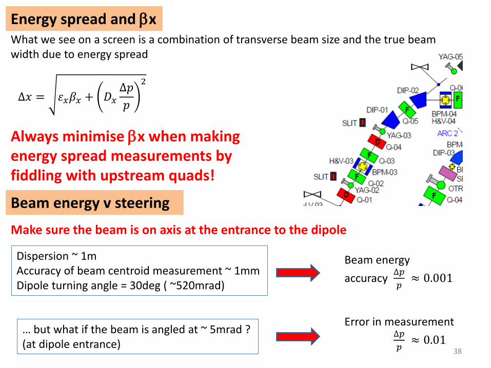
Energy spread and bx What we see on a screen is a combination of transverse beam size and the true beam width due to energy spread

∆𝑥 = 휀𝑥𝛽𝑥 + 𝐷𝑥

∆𝑝

𝑝

2

Always minimise bx when making energy spread measurements by fiddling with upstream quads!

Beam energy v steering

Make sure the beam is on axis at the entrance to the dipole

Dispersion ~ 1m Accuracy of beam centroid measurement ~ 1mm Dipole turning angle = 30deg ( ~520mrad)

Beam energy

accuracy ∆𝑝

𝑝 ≈ 0.001

… but what if the beam is angled at ~ 5mrad ? (at dipole entrance)

Error in measurement

∆𝑝

𝑝 ≈ 0.01

38

Beam physics is always a bit more complicated than we wish to think

This is a topic for many more lectures We will not discuss it here … only a few examples

39

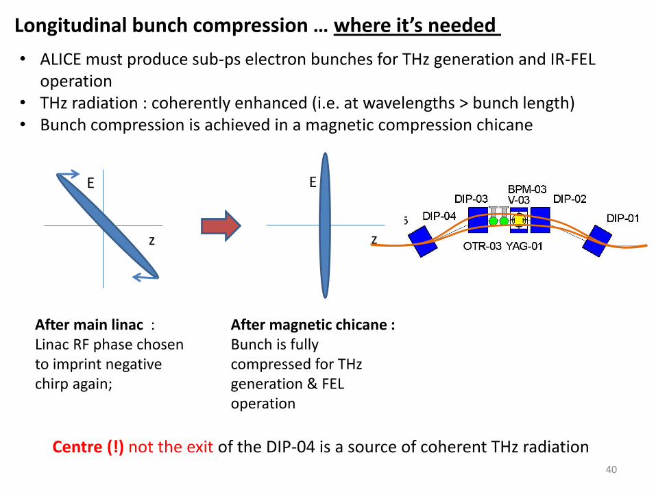
Longitudinal bunch compression … where it’s needed

• ALICE must produce sub-ps electron bunches for THz generation and IR-FEL operation

• THz radiation : coherently enhanced (i.e. at wavelengths > bunch length) • Bunch compression is achieved in a magnetic compression chicane

z

E

After main linac : Linac RF phase chosen to imprint negative chirp again;

z

E

After magnetic chicane : Bunch is fully compressed for THz generation & FEL operation

Centre (!) not the exit of the DIP-04 is a source of coherent THz radiation 40

Longitudinal bunch compression … where it’s needed

Main linac off-crest phase is chosen such that it introduces a linear negative energy chirp along the bunch that is perfectly matched to R56 between the linac and the chicane exit

1

𝐸0

𝑑𝐸

𝑑𝑧= −

1

𝑅56

∆𝑙 = 𝑅51𝑥0 + 𝑅52𝑥0′ + 𝑅53𝑦 + 𝑅54𝑦0

′ + 𝑅56

∆𝑝

𝑝0

Now, here is the complication : transverse beam dynamics may play a role as well !!

THz

THz Bunch is fully compressed longitudinally but “skewed” wrt the beam trajectory effective bunch lengthening

Both R51 and R52 normally ≠ 0 in the middle of the last dipole of the chicane

Now add second order (T566) and even higher order components to get a perfect headache 41

Other things that may come into play (certainly far from being a complete list !!! ) • Space charge - at what beam energy we can forget about it ? - quad scans: will they be affected ? (certainly at < 10MeV at some extent)

• How relativistic is the beam ? - e.g. shall we remember about velocity bunching/de-bunching ?

E=6.5MeV (ALICE injector energy) 𝛾 = 13.72 𝛽 = 0.9973

∆𝑧 =∆𝛽

𝛽𝑠 ∆𝛽 =

∆𝐸

𝑚𝑐2𝛽𝛾3

s ~ 15m; ∆𝐸 ~ 100keV

∆𝑧 ≈ 1𝑚𝑚 ≈ 3𝑝𝑠

That’s large enough to be worry about !

• Phase slippage (initial stages of acceleration in booster) - could be huge if relatively low energy beams accelerated at high RF gradients

∆𝜑 ≈ 180𝑜1 − 𝛽

𝛽

Crude estimate of phase slippage in one cell of RF cavity assuming (i) π-mode ; (ii) no energy change; (iii) cavity designed for fully relativistic beams

240keV (old ALICE gun voltage) ∆𝜑 ≈ 60𝑜 42

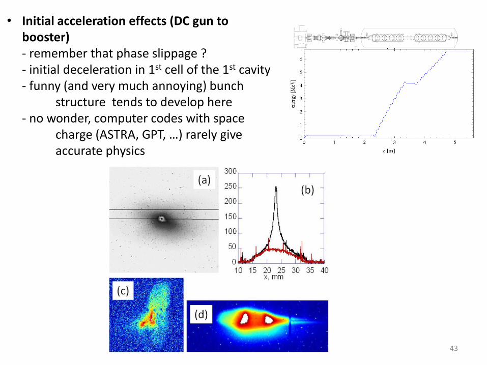
• Initial acceleration effects (DC gun to booster)

- remember that phase slippage ? - initial deceleration in 1st cell of the 1st cavity - funny (and very much annoying) bunch structure tends to develop here - no wonder, computer codes with space charge (ASTRA, GPT, …) rarely give accurate physics

43

A few final notes

… in case, up until now, you not scared enough of experimental accelerator physics

44

• Never take whatever you measure “at face value” check, double check and cross-check everything • Avoid temptation to explain some anomaly you see in experimental data by

invoking a “fancy theory” in most cases, the truest explanation is the simplest one • Do not expect your machine to be absolutely stable (daily or even hourly, in

some cases, drifts can happen !) - if your measurements span over a few hours (or even days), make sure the machine is not drifted - make regular checks - repeat initial measurement after the last one is completed

• Know your machine as “wide” as possible - “wide” means knowledge of how different things are made and operate and some basic physics of any process present in the machine

• Do not introduce new mistakes while analysing experimental data - you’ve already made enough of them while collecting data

Sort of summary

45

Experimental physicist : • Is not expected to be an expert in everything but should have enough knowledge of

every machine system and sub-system (high power RF, LLRF, lasers, vacuum, cryo etc.) • Cannot be in full control of machine development but has to influence it from his/her

own perspective • Need to know accelerator physics by “fingertips” (i.e. able to explain everything with a

piece of scrap paper and a pencil) • Need to know / be aware of different pitfalls in experimental practice • And still need to have lots of expertise in computer simulation codes (you cannot always

rely on others to do these things for you !) • Most likely has to operate the machine (and not only for his own pet projects )

What is the experimental accelerator physicist ? (my personal views)

All of the above = hard work + lots of time invested + dedication

Must have because most of the outcome is not particularly “publishable”

And a reward ? • Huge satisfaction in that you and your colleagues made this machine work ! • Continuous stream of small discoveries that you will make while working with the

machine

Probably, that’s why experimentalists do not write books …

46