Embed Size (px)
Citation preview
Acceleration, Braking, and Steering Controller for Polaris GEM e2
by
Matthew Benton Salfer-Hobbs
Bachelor of ScienceMechanical Engineering
Florida Institute of Technology2017
A thesissubmitted to the College of Engineering
at Florida Institute of Technologyin partial fulfillment of the requirements
for the degree of
Master of Sciencein
Mechanical Engineering
Melbourne, FloridaMay, 2019

c⃝ Copyright 2019 Matthew Benton Salfer-Hobbs
All Rights Reserved
The author grants permission to make single copies.
We the undersigned committeehereby approve the attached thesis
Acceleration, Braking, and Steering Controller for Polaris GEM e2by Matthew Benton Salfer-Hobbs
Matthew Jensen, Ph.D.Assistant ProfessorMechanical EngineeringCommittee Chair
Anthony Smith, Ph.D.Assistant ProfessorElectrical and Computer EngineeringOutside Committee Member
Hector Gutierrez, Ph.D.ProfessorMechanical EngineeringCommittee Member
Ashok Pandit, Ph.D.Professor and Department HeadMechanical and Civil Engineering
ABSTRACT
Title:
Acceleration, Braking, and Steering Controller for Polaris GEM e2
Author:
Matthew Benton Salfer-Hobbs
Major Advisor:
Matthew Jensen, Ph.D.
This paper discusses the design and simulation of lane keeping and velocity con-
trollers for a Polaris GEM e2. The controllers were designed to be implemented in
Florida Institute of Technology’s entry for the Intelligent Ground Vehicle Compe-
tition self-drive challenge. The software and physical implementation of actuators
were included to control the acceleration, braking, and steering. The accelerator
pedal was replaced with a set of digitally controlled potentiometers, the brake
pedal was replaced with a linear actuator, and the steering column was replaced
with a stepper motor. Each actuator was controlled by a Raspberry Pi 3. A slid-
ing mode controller was designed and its performance was evaluated against a PID
controller for lane keeping. The sliding mode controller had a consistently smaller
lateral error, especially during changes to the radius of the curve. Velocity control
was simulated using a derived dynamic model for the longitudinal motion of the
car. An adaptive control method was designed for velocity control and compared
to PID. The adaptive control method reduced the error in longitudinal position
during both acceleration and deceleration.
iii
Table of Contents
Abstract iii
List of Figures vii
List of Tables x
Acknowledgments xi
Dedication xii
1 Introduction 1
1.1 Background Information . . . . . . . . . . . . . . . . . . . . . . . . 1
1.1.1 Automotive Safety . . . . . . . . . . . . . . . . . . . . . . . 1
1.1.2 Levels of Autonomous Driving . . . . . . . . . . . . . . . . . 3
1.1.3 Control Systems . . . . . . . . . . . . . . . . . . . . . . . . . 6
1.2 Objectives . . . . . . . . . . . . . . . . . . . . . . . . . . . . . . . . 7
1.3 Importance of Study . . . . . . . . . . . . . . . . . . . . . . . . . . 8
2 Literature Review 10
2.1 Definitions of Variables and Axes . . . . . . . . . . . . . . . . . . . 10
2.2 Kinematic and Dynamic Models . . . . . . . . . . . . . . . . . . . . 12
2.2.1 2 DOF Model . . . . . . . . . . . . . . . . . . . . . . . . . . 13
iv
2.2.2 3 DOF Model . . . . . . . . . . . . . . . . . . . . . . . . . . 14
2.2.3 5 DOF Model . . . . . . . . . . . . . . . . . . . . . . . . . . 16
2.2.4 8 DOF Model and Higher . . . . . . . . . . . . . . . . . . . 16
2.3 Control Systems . . . . . . . . . . . . . . . . . . . . . . . . . . . . . 17
2.3.1 PID Controllers . . . . . . . . . . . . . . . . . . . . . . . . . 19
2.3.2 Fuzzy Logic . . . . . . . . . . . . . . . . . . . . . . . . . . . 21
2.3.3 Adaptive Controller . . . . . . . . . . . . . . . . . . . . . . . 23
2.3.4 Sliding Mode Controller . . . . . . . . . . . . . . . . . . . . 25
2.4 ROS . . . . . . . . . . . . . . . . . . . . . . . . . . . . . . . . . . . 27
2.4.1 Communication Framework . . . . . . . . . . . . . . . . . . 27
3 Methodology 29
3.1 Overview of Polaris GEM e2 . . . . . . . . . . . . . . . . . . . . . . 29
3.2 Control Systems Overview . . . . . . . . . . . . . . . . . . . . . . . 30
3.3 Accelerator Control . . . . . . . . . . . . . . . . . . . . . . . . . . . 32
3.4 Brake Control . . . . . . . . . . . . . . . . . . . . . . . . . . . . . . 35
3.5 Steering Angle Control . . . . . . . . . . . . . . . . . . . . . . . . . 38
3.6 Kinematic Model for Simulations . . . . . . . . . . . . . . . . . . . 41
3.7 Dynamic Model for Longitudinal Motion . . . . . . . . . . . . . . . 42
3.8 Velocity Control Methods . . . . . . . . . . . . . . . . . . . . . . . 46
3.8.1 PID Control . . . . . . . . . . . . . . . . . . . . . . . . . . . 46
3.8.2 Adaptive Control . . . . . . . . . . . . . . . . . . . . . . . . 47
3.8.3 Simulated Paths . . . . . . . . . . . . . . . . . . . . . . . . . 49
3.9 Lane Keeping Control Methods . . . . . . . . . . . . . . . . . . . . 51
3.9.1 PID Control . . . . . . . . . . . . . . . . . . . . . . . . . . . 51
3.9.2 Sliding Control . . . . . . . . . . . . . . . . . . . . . . . . . 52
v
3.9.3 Simulated Path . . . . . . . . . . . . . . . . . . . . . . . . . 53
4 Results 56
4.1 Velocity Control . . . . . . . . . . . . . . . . . . . . . . . . . . . . . 56
4.1.1 Acceleration . . . . . . . . . . . . . . . . . . . . . . . . . . . 56
4.1.2 Deceleration . . . . . . . . . . . . . . . . . . . . . . . . . . . 59
4.2 Lane Keeping . . . . . . . . . . . . . . . . . . . . . . . . . . . . . . 62
4.2.1 Decreasing Radius . . . . . . . . . . . . . . . . . . . . . . . 62
4.2.2 Step Input . . . . . . . . . . . . . . . . . . . . . . . . . . . . 64
4.2.3 Sinusoidal Curve . . . . . . . . . . . . . . . . . . . . . . . . 65
5 Conclusions and Future Work 67
5.1 Conclusions . . . . . . . . . . . . . . . . . . . . . . . . . . . . . . . 67
5.2 Future Work . . . . . . . . . . . . . . . . . . . . . . . . . . . . . . . 68
5.2.1 Increasing DOF . . . . . . . . . . . . . . . . . . . . . . . . . 68
5.2.2 System Integration . . . . . . . . . . . . . . . . . . . . . . . 69
5.2.3 Revise Sliding Mode Controller . . . . . . . . . . . . . . . . 69
5.2.4 Utilize Fuzzy Logic . . . . . . . . . . . . . . . . . . . . . . . 69
References 71
vi
List of Figures
1.1 Stanley, the 2005 DARPA Grand Challenge winner, [17] . . . . . . . 3
1.2 Example of adaptive cruise control. Car 1 maintains a safe distance
from the car 2 using on-board sensors. . . . . . . . . . . . . . . . . 4
1.3 Simple diagram of a feedback control loop . . . . . . . . . . . . . . 7
2.1 Vehicle fixed coordinate system, [18] . . . . . . . . . . . . . . . . . 11
2.2 Dynamic model of a vehicle, [47] . . . . . . . . . . . . . . . . . . . . 13
2.3 2DOF model of a bicycle, [40] . . . . . . . . . . . . . . . . . . . . . 14
2.4 3DOF model of a vehicle, [42] . . . . . . . . . . . . . . . . . . . . . 15
2.5 Model of tire slip angle, [36] . . . . . . . . . . . . . . . . . . . . . . 16
2.6 8 DOF model of a vehicle, [11] . . . . . . . . . . . . . . . . . . . . . 17
2.7 Structure of multi-vehicle adaptive cruise control, [41] . . . . . . . . 18
2.8 Diagram of a PID control loop, [15] . . . . . . . . . . . . . . . . . . 19
2.9 Response of a PID system, [24] . . . . . . . . . . . . . . . . . . . . 20
2.10 Budapest University autonomous go-cart, [9] . . . . . . . . . . . . . 21
2.11 Rule table for fuzzy logic controller, [56] . . . . . . . . . . . . . . . 23
2.12 Difference between Sign and Sat function, [14] . . . . . . . . . . . . 26
2.13 Example of ROS publisher and subscriber setup. . . . . . . . . . . . 28
3.1 Polaris GEM e2, [38] . . . . . . . . . . . . . . . . . . . . . . . . . . 29
vii
3.2 Controller architecture. . . . . . . . . . . . . . . . . . . . . . . . . . 31
3.3 Diagram of axis labels for Xbox 360 controller using ROS joy package. 32
3.4 Pinout of the accelerator sensor, courtesy of Polaris. . . . . . . . . . 33
3.5 Signals received by the Accelerator sensor, courtesy of Polaris. . . . 33
3.6 Wiring Diagram for accelerator control. . . . . . . . . . . . . . . . . 35
3.7 ARM66SMK stepper motor with linear actuator. . . . . . . . . . . 36
3.8 ARD-KD closed loop motor driver. . . . . . . . . . . . . . . . . . . 36
3.9 Wiring diagram for braking controller. . . . . . . . . . . . . . . . . 37
3.10 Trinamic PD 86-3-1180 with gearbox side view. . . . . . . . . . . . 38
3.11 Trinamic PD 86-3-1180 with gearbox front view. The driving gear
is shown in blue, and the driven gear is shown in red. . . . . . . . . 39
3.12 Position error for PID control of stepper motor due to step input. . 40
3.13 Position error for PID control of stepper motor due to ramp input. . 40
3.14 Forces acting on car for longitudinal motion. . . . . . . . . . . . . . 44
3.15 PID tuning for velocity control. . . . . . . . . . . . . . . . . . . . . 47
3.16 Desired velocity of vehicle during acceleration simulation. . . . . . . 49
3.17 Desired position of vehicle during acceleration simulation. . . . . . . 50
3.18 Desired velocity of vehicle during deceleration simulation. . . . . . . 50
3.19 Desired position of vehicle during acceleration simulation. . . . . . . 51
3.20 PID tuning for steering. . . . . . . . . . . . . . . . . . . . . . . . . 52
3.21 Desired path of vehicle during decreasing radius lane keeping simu-
lation. . . . . . . . . . . . . . . . . . . . . . . . . . . . . . . . . . . 54
3.22 Desired radius of vehicle during decreasing radius lane keeping sim-
ulation. . . . . . . . . . . . . . . . . . . . . . . . . . . . . . . . . . 54
3.23 Desired path of vehicle during sinusoidal lane keeping simulation. . 55
viii
4.1 Position of PID and adaptive controller during acceleration. The
desired position is covered by the adaptive controller. . . . . . . . . 57
4.2 Velocity of PID and adaptive controller during acceleration. The
desired velocity is covered by the adaptive controller. . . . . . . . . 57
4.3 Position error for PID and Adaptive controller during acceleration. 58
4.4 Velocity error for PID and Adaptive controller during acceleration. . 58
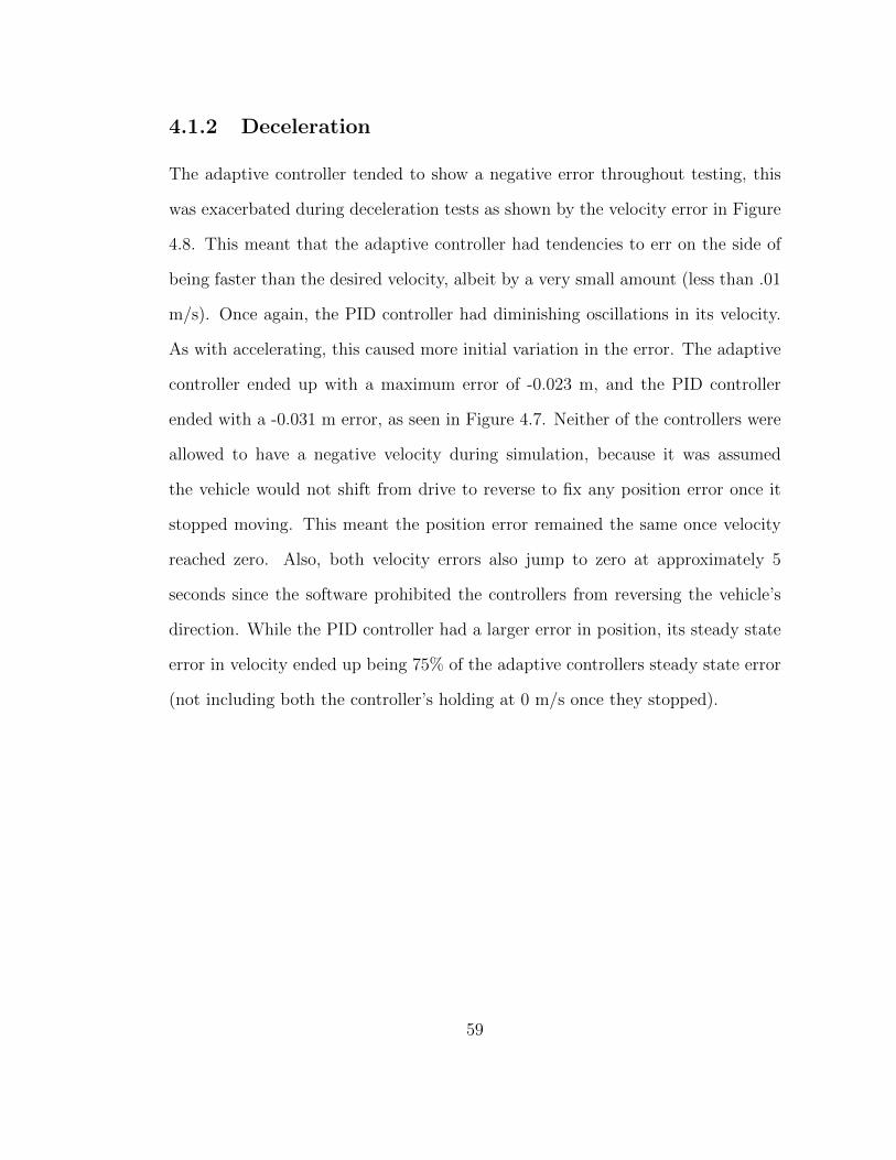
4.5 Position of PID and adaptive controller during deceleration. The
desired position is covered by the adaptive controller. . . . . . . . . 60
4.6 Velocity of PID and adaptive controller during deceleration.The de-
sired velocity is covered by the adaptive controller. . . . . . . . . . 60
4.7 Position error for PID and Adaptive controller during deceleration. 61
4.8 Velocity error for PID and Adaptive controller during deceleration. 61
4.9 Position of vehicle during decreasing radius turn. . . . . . . . . . . 63
4.10 Lateral Error for PID and Sliding control during decreasing radius
turn. . . . . . . . . . . . . . . . . . . . . . . . . . . . . . . . . . . . 63
4.11 Steering angle during lane keeping simulation. the paths overlap
each other for the majority of the simulation. . . . . . . . . . . . . 64
4.12 Lateral position for PID and Sliding controller after step input of 1m. 65
4.13 Position of vehicle during sinusoidal path. Sliding control is over-
lapping the desired path. . . . . . . . . . . . . . . . . . . . . . . . 66
4.14 Lateral Error for PID and Sliding control during sinusoidal path. . . 66
ix
List of Tables
3.1 Polaris GEM e2 Specifications [38] . . . . . . . . . . . . . . . . . . 30
3.2 Voltage and potentiometer settings for accelerator control. Digital
(1) and (2) show the values sent to each potentiometer. . . . . . . . 34
3.3 Values used for velocity simulation. . . . . . . . . . . . . . . . . . . 46
x
Acknowledgements
I am thankful for my parents and for their continuing support of my education.
They helped to give me countless opportunities and learning experiences. I would
like to thank Dr. Matthew Jensen for guiding and mentoring me through my
Bachelors and Masters program at Florida Institute of Technology. I would also
like to thank Magna and Polaris funding and supporting Florida Tech’s IGVC
team. Lastly, I would like to thank Thomas LaPointe, who introduced me to the
world of robotics.
xi
Dedication
This paper is dedicated to Victoria Bruce. Her support during all the late nights
spent running simulations and writing has not gone unnoticed.
xii
Chapter 1
Introduction
1.1 Background Information
1.1.1 Automotive Safety
Autonomous vehicles are a largely researched topic with a wide public following.
While the history of the automobile is relatively brief, it has quickly become a
necessity. Approximately 95 percent of households in the United States own at
least one car and 85 percent of Americans commute to work via car [12]. As
integral as driving has become to daily life, it still carries a variety of risks. In
2015, at least 2,338,000 injuries and 35,000 deaths were related to car accidents in
the United States [3]. These values remain high, even though a variety of safety
measures have been implemented since the inception of public driving. Examples
of these safety measures include: New York becoming the first state to ban drunk
driving in 1910, the application of the three-way traffic light in 1930, and the
development of airbags and seatbelts in the 1950s [2]. Various agencies were also
1
formed in response to the necessity of driving, including the establishment of the
Department of Transportation in 1967 and the National Highway Traffic Safety
Administration in 1970 [2].
Each of these initiatives have aided in preventing automobile related deaths.
However, death is still a prominent risk of driving. However, a major risk factor
that none of these initiatives can prevent is human error. Approximately 94 percent
of major accidents are caused by human error, such as distraction and slow reaction
times [4]. This has resulted in a wide public interest in developing fully automated
vehicles. In addition to reducing human fatalities, autonomy also bears economic
benefits. Within the United States alone, the estimated economic cost of all traffic
related crashes was $242 billion in 2010 [5]. Also, the efficiency of traffic would
improve, leading to smoother and faster traffic flow [19].
Research into autonomous vehicle gained more popularity in 2002 when the
Defense Advanced Research Projects Agency (DARPA) developed the DARPA
Grand Challenge. This challenge was designed to further develop the field of
autonomous vehicles by offering $1 million to a team that would design a vehicle
that could drive itself though a desert course. This first iteration of this challenge
was in 2004 and it yielded no successful vehicles. Then in 2005, the Stanford
Racing Teams vehicle (shown in Figure 1.1) was able to complete the challenge
by navigating 132 miles of terrain in less than 7 hours. In 2007, Carnegie Melon
University completed the DARPA Urban Challenge, which made use of a more
conventional city-styled course [6]. The most recently developed challenge is the
Intelligent Ground Vehicle Competition (IGVC) Self-Drive Challenge, which will
help autonomous vehicles evolve further with the current available technology.
2
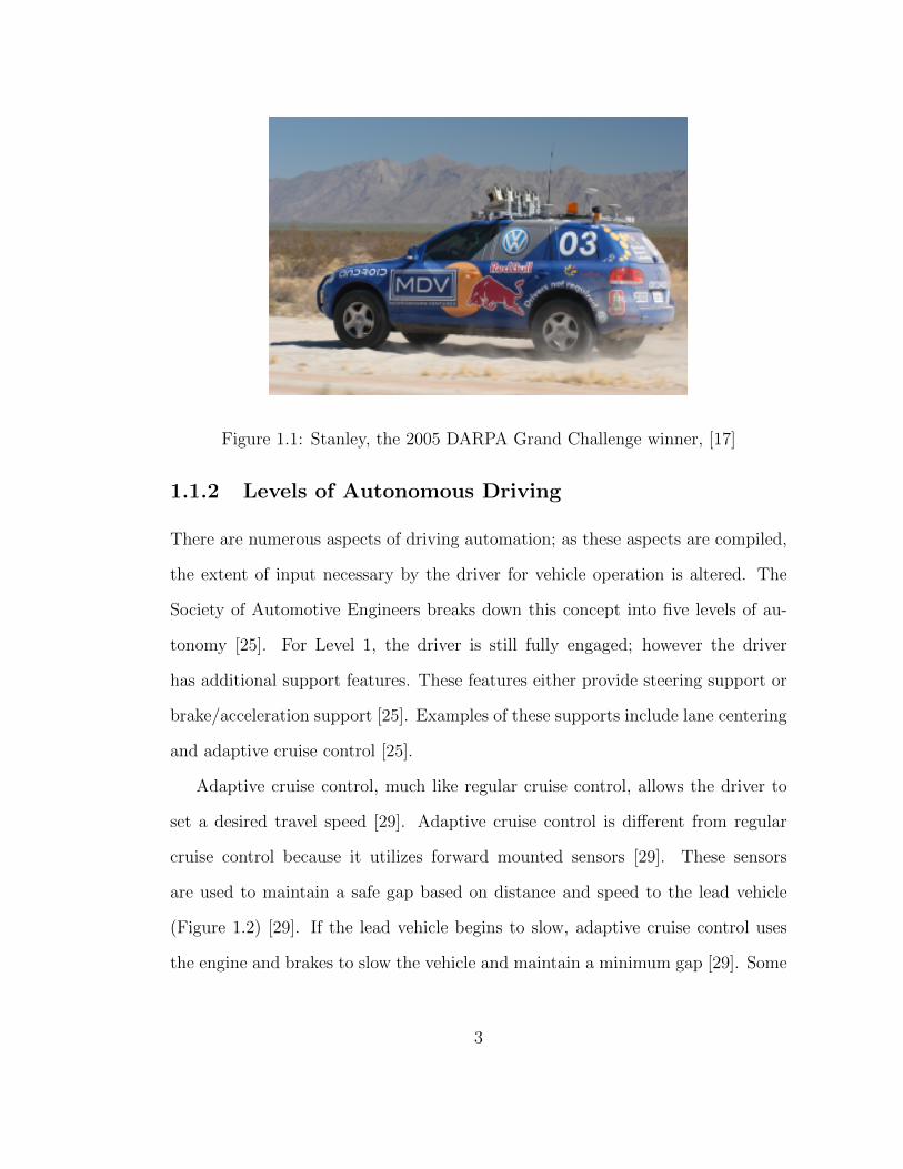
Figure 1.1: Stanley, the 2005 DARPA Grand Challenge winner, [17]
1.1.2 Levels of Autonomous Driving
There are numerous aspects of driving automation; as these aspects are compiled,
the extent of input necessary by the driver for vehicle operation is altered. The
Society of Automotive Engineers breaks down this concept into five levels of au-
tonomy [25]. For Level 1, the driver is still fully engaged; however the driver
has additional support features. These features either provide steering support or
brake/acceleration support [25]. Examples of these supports include lane centering
and adaptive cruise control [25].
Adaptive cruise control, much like regular cruise control, allows the driver to
set a desired travel speed [29]. Adaptive cruise control is different from regular
cruise control because it utilizes forward mounted sensors [29]. These sensors
are used to maintain a safe gap based on distance and speed to the lead vehicle
(Figure 1.2) [29]. If the lead vehicle begins to slow, adaptive cruise control uses
the engine and brakes to slow the vehicle and maintain a minimum gap [29]. Some
3
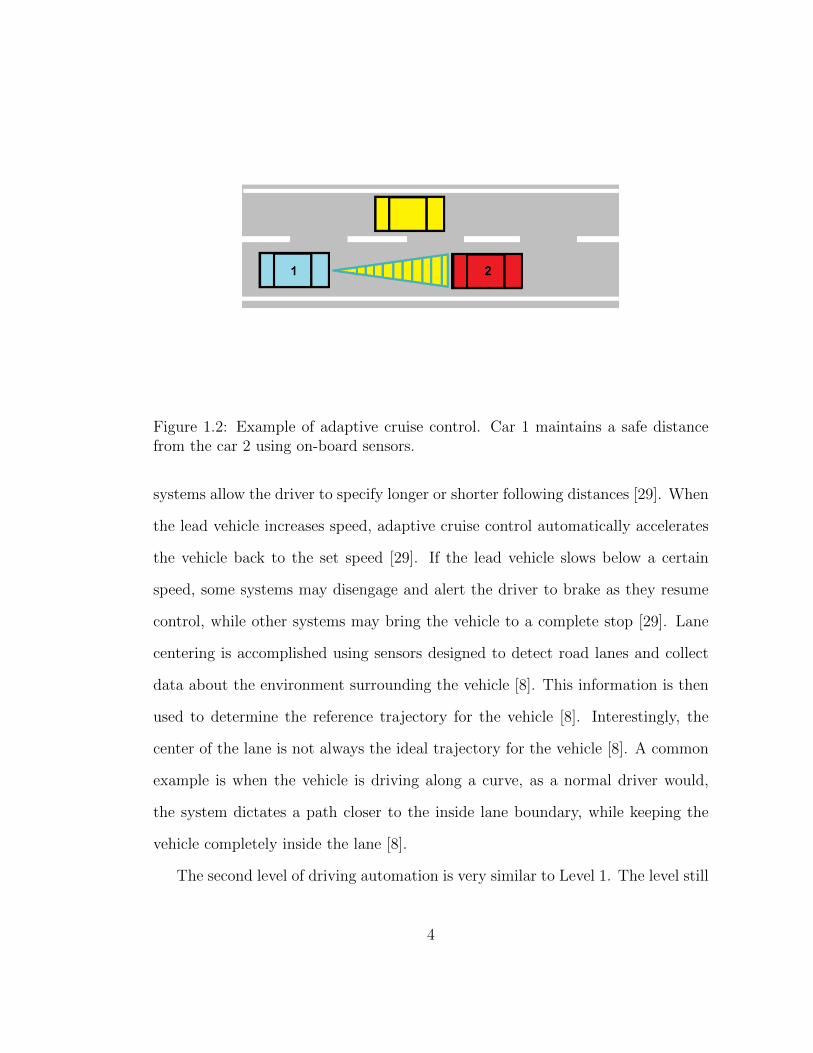
Figure 1.2: Example of adaptive cruise control. Car 1 maintains a safe distancefrom the car 2 using on-board sensors.
systems allow the driver to specify longer or shorter following distances [29]. When
the lead vehicle increases speed, adaptive cruise control automatically accelerates
the vehicle back to the set speed [29]. If the lead vehicle slows below a certain
speed, some systems may disengage and alert the driver to brake as they resume
control, while other systems may bring the vehicle to a complete stop [29]. Lane
centering is accomplished using sensors designed to detect road lanes and collect
data about the environment surrounding the vehicle [8]. This information is then
used to determine the reference trajectory for the vehicle [8]. Interestingly, the
center of the lane is not always the ideal trajectory for the vehicle [8]. A common
example is when the vehicle is driving along a curve, as a normal driver would,
the system dictates a path closer to the inside lane boundary, while keeping the
vehicle completely inside the lane [8].
The second level of driving automation is very similar to Level 1. The level still
4
expects the driver to be fully engaged and supervise the support systems, however
both steering and acceleration support are supplied to the driver simultaneously
[25]. Examples of implementations that have been available for public use include
Teslas Autopilot, Cadillac Super Cruise, Volvo Pilot Assist, and others [1].
The features that are implemented in Levels 3 and 4 are both capable of driving
the vehicle under restricted conditions, and these systems will only operate when
all of the specified conditions are met [25]. For both of these levels, when the system
is enacted the driver is not in any control of the vehicle; the vehicle is capable of
speeding up, slowing down, passing slower cars, and making emergency decisions
such as swerving or braking [4]. The major difference between Levels 3 and 4 is
that Level 3 still needs the driver to be monitoring the system, because when the
system requests it, the driver must resume driving and take over all controls [25].
Meanwhile, Level 4 will not require the driver to take over the controls [25]. Level
4 may request for the driver to take over the controls, however if the driver does
not take over, the vehicle will safely pull off of the road and come to a complete
stop until the driver acknowledges the request to take over the controls [4]. Due
to the possible risks associated with Level 3, many manufacturers, such as Volvo,
tend to implement Level 2 or Level 4 systems [13]. Conversely, other companies,
including Audi, already implement Level 3 systems, since they believe that the
benefits of the system outweigh the risks [13].
The fifth level of autonomous driving represents full automation [25]. The fea-
tures for this level are the same as Level 4, however Level 5 is capable of automated
driving under all conditions and it will never request for the driver to take over
controls [25]. This level of automation is expected to be in use as early as the
mid-2020s [4]. A prominent challenge to reaching Level 5 is developing a control
5
system that has the ability to quickly use information from its sensors to design,
update and execute the safest possible path. As of 2018, 73 percent of drivers in
the United States fear riding in fully autonomous vehicles [1], this is likely due to
fatalities associated with the technology that were widely publicized. This further
proves the necessity of designing the systems to be extremely reliable as a means
to alleviate public concern.
1.1.3 Control Systems
Control systems have a vast history; the earliest example dating back over 2000
years to the water clocks described by Vitruvius and Ktesibios [10]. More com-
plex controllers emerged as devices increased in complexity over time. In the
early 1900s, feedback controllers became common for the regulation of various sys-
tems, such as voltages and planes. Simultaneously, proportional-integral-derivative
(PID) controllers with automatic gain adjustment were integrated into the steering
systems of ships in order to adjust automatically to sea conditions [10].
A simplified model of a feedback controls system includes the controller, the
system, and its outputs (Figure 1.3). Sensors are in place to aid in determining
the error between the desired values and the measured values. The determined
error is then used by the controller to generate an input to the system towards
correcting the error [16]. Certain controllers utilize a system model that predicts
the reaction of the physical system and account for it in the generated inputs.
6
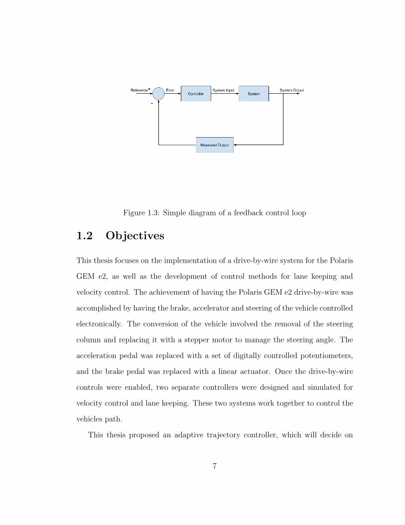
Figure 1.3: Simple diagram of a feedback control loop
1.2 Objectives
This thesis focuses on the implementation of a drive-by-wire system for the Polaris
GEM e2, as well as the development of control methods for lane keeping and
velocity control. The achievement of having the Polaris GEM e2 drive-by-wire was
accomplished by having the brake, accelerator and steering of the vehicle controlled
electronically. The conversion of the vehicle involved the removal of the steering
column and replacing it with a stepper motor to manage the steering angle. The
acceleration pedal was replaced with a set of digitally controlled potentiometers,
and the brake pedal was replaced with a linear actuator. Once the drive-by-wire
controls were enabled, two separate controllers were designed and simulated for
velocity control and lane keeping. These two systems work together to control the
vehicles path.
This thesis proposed an adaptive trajectory controller, which will decide on
7
a percentage of actuation for the brake and accelerator in order to maintain or
change its speed. Adaptive trajectory control allows the controller to be robust to
unknown and changing parameters, such as road conditions [55]. As a comparison,
a PID controller was also designed. These two methods were both applied to a
model of the vehicle travelling in a straight line. The tracking accuracy of both
position and velocity were evaluated. This thesis also examined the usefulness of a
sliding mode controller for lane keeping. A sliding mode controller works to reduce
the tracking error to zero by driving the system onto a sliding surface in state
space [14]. The sliding mode control was compared to a PID controller using a 2
degree of freedom bicycle style model.
The resulting vehicle would have the ability to accelerate and maintain a speed
limit, follow a reference trajectory, and brake within a safe distance. Additionally,
the resulting system will provide an autonomous platform for researchers to test
their own sensors and path planning algorithms by simplifying the necessary inputs
to the controller.
1.3 Importance of Study
The purpose of this thesis is to establish steering, brake, and acceleration control
that can easily be set up and used on autonomous vehicles. This system is ex-
pected to be used for Florida Institute of Technology’s Intelligent Ground Vehicle
Competition (IGVC) entry. Research on self-driving cars is still an expanding field.
Various controllers such as PID, non-linear, and adaptive have been proposed pre-
viously for lane keeping [57] [43] [9]. Previous research has shown that various
forms of PID controllers work for velocity control [21] [9]. Fuzzy logic has also
8
been proposed for accelerating and braking [33] [56]. Currently, the proposed slid-
ing mode controller for lane keeping and adaptive trajectory controller for velocity
have not yet been widely examined.
As of July 2018, it has been estimated that autonomous vehicles could con-
tribute $2 trillion to the U.S. economy by 2050 [1]. In turn, by 2030 is has also
been forecasted that the car data industry could be appreciated at $750 million
[1]. Currently, most of the autonomous vehicles that populate public streets are
driverless shuttles [1]. Many implementations of this are already planned across the
United States, while cities like Las Vegas, NV and San Ramon, CA already have
driverless shuttles in regular use on public streets [1]. It has also been predicted
that there will be a need for autonomous vehicles for our vastly growing elderly
population [1]. In 2050, there is projected to be 83.7 million Americans over the
age of 65 and currently nearly one-third of states do not yet have autonomous
vehicle legislation or executive orders set [1].
There is a need for testing platforms that can be quickly adapted to test new
ideas. The control algorithm and physical implementation proposed in this thesis
would provide a straight forward hardware and software setup that would allow
researchers to shift their focus to higher level tasks such as designing an AI for
path planning in emergencies or fusing different sensor data together to perform
fast and accurate object detection and classification.
9
Chapter 2
Literature Review
2.1 Definitions of Variables and Axes
The Society of Automotive Engineers (SAE) uses standard terminology to describe
the vehicles motion both locally and globally. These definitions are based off of
SAE-J670.
Earth-Fixed Axis System: This is a fixed-reference system denoted by X, Y,
and Z. The origin for this coordinate system is chosen by the user, and
is attached to the ground. X and Y make up the ground plane, and Z is
the vertical plane [34].
Vehicle Axis System: This is a reference system that is fixed to the center of
gravity (COG) of the vehicle, and is denoted by x, y, and z (Figure 2.1).
The coordinate system is orthogonal and right-handed. The x-axis of the
vehicle points in the forward direction of motion and horizontal when
the vehicle is travelling in a straight line on flat terrain. The y-axis is
also horizontal, and is 90 degrees from the x-axis. This points the y-axis
10
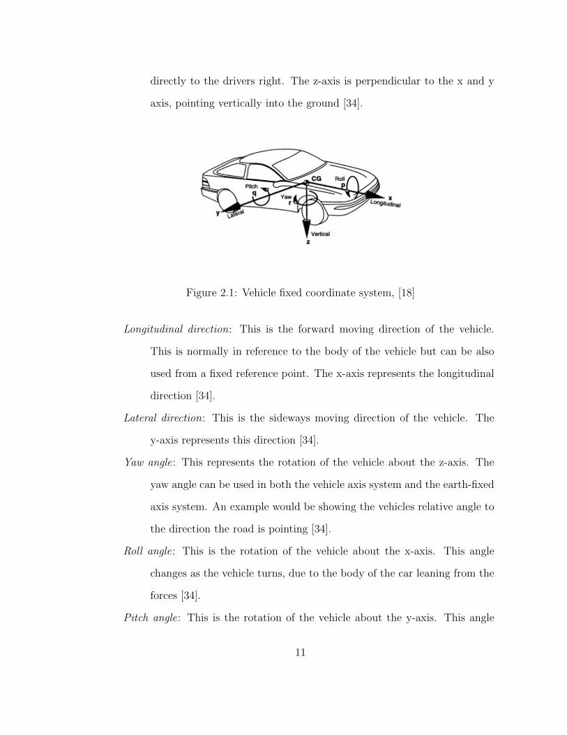
directly to the drivers right. The z-axis is perpendicular to the x and y
axis, pointing vertically into the ground [34].
Figure 2.1: Vehicle fixed coordinate system, [18]
Longitudinal direction: This is the forward moving direction of the vehicle.
This is normally in reference to the body of the vehicle but can be also
used from a fixed reference point. The x-axis represents the longitudinal
direction [34].
Lateral direction: This is the sideways moving direction of the vehicle. The
y-axis represents this direction [34].
Yaw angle: This represents the rotation of the vehicle about the z-axis. The
yaw angle can be used in both the vehicle axis system and the earth-fixed
axis system. An example would be showing the vehicles relative angle to
the direction the road is pointing [34].
Roll angle: This is the rotation of the vehicle about the x-axis. This angle
changes as the vehicle turns, due to the body of the car leaning from the
forces [34].
Pitch angle: This is the rotation of the vehicle about the y-axis. This angle
11
changes as the vehicle accelerates or decelerates [34].
Steering angle: This is the angle between the direction the front of the vehicle
is pointing and the direction the steered wheels are pointing. Looking at
the x-y plane of the vehicle coordinate system, this angle is zero when
aligned with the x-axis [34].
Body slip angle: This is the angle between the vehicles velocity vector and
longitudinal direction [34].
2.2 Kinematic and Dynamic Models
An accurate model is necessary for providing controls and simulations of a vehi-
cle. The model can vary in complexity to meet the demands of the simulation.
Primarily, the differences between the various models are the number of degrees of
freedom (DOF) and the assumptions made to complete the model. In this case,
DOF refers to the directions the vehicle can move and rotate, as well as how the
internal parts such as suspension can move. There are six DOF that govern how
the vehicle moves. The vehicle can travel longitudinally, or in the direction of its
length (x-axis). It can also travel laterally, which perpendicular to the longitudinal
direction (y-axis). The third axis is vertical (z-axis). All three of these axes also
can be rotated around. The longitudinal axis allows for roll, the lateral axis allows
for pitch, and the vertical axis allows for yaw [47]. These 6 motions explain the
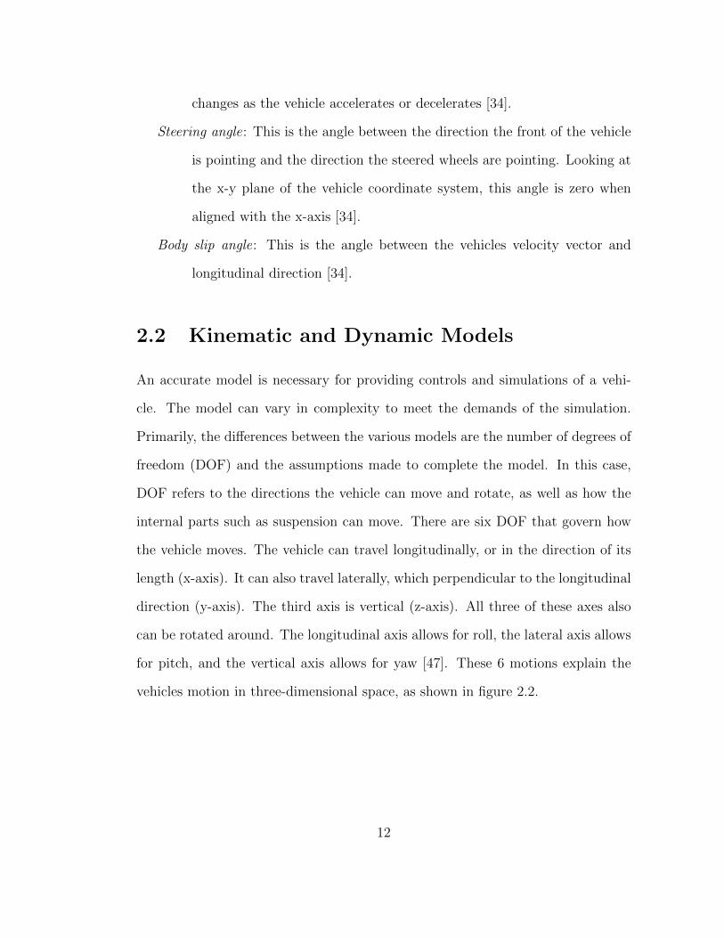
vehicles motion in three-dimensional space, as shown in figure 2.2.
12
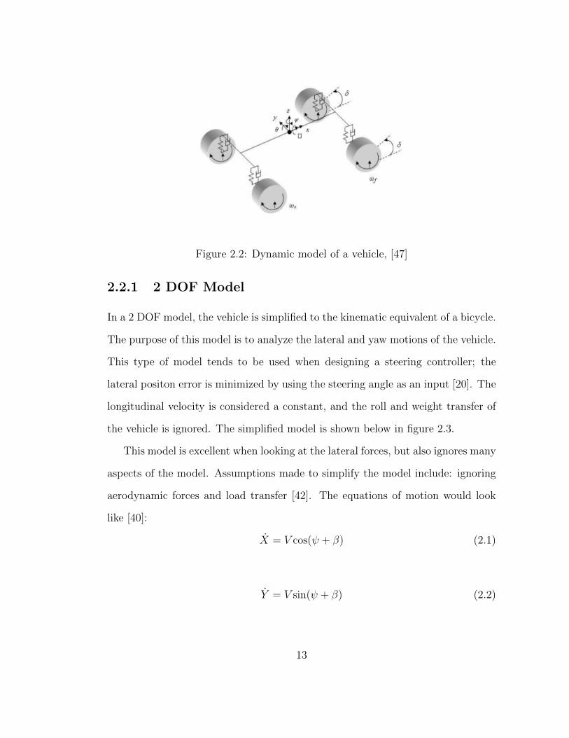
Figure 2.2: Dynamic model of a vehicle, [47]
2.2.1 2 DOF Model
In a 2 DOF model, the vehicle is simplified to the kinematic equivalent of a bicycle.
The purpose of this model is to analyze the lateral and yaw motions of the vehicle.
This type of model tends to be used when designing a steering controller; the
lateral positon error is minimized by using the steering angle as an input [20]. The
longitudinal velocity is considered a constant, and the roll and weight transfer of
the vehicle is ignored. The simplified model is shown below in figure 2.3.
This model is excellent when looking at the lateral forces, but also ignores many
aspects of the model. Assumptions made to simplify the model include: ignoring
aerodynamic forces and load transfer [42]. The equations of motion would look
like [40]:
X = V cos(ψ + β) (2.1)
Y = V sin(ψ + β) (2.2)
13
ψ =V cos(β)
ℓf + ℓr(tan(δf )− tan(δr)) (2.3)
These equations can be simplified down further with the assumption that the
rear tires remain aligned with the longitudinal axis. Therefore, δr can be set to 0,
simplifying equation 2.3 to [40]:
ψ =V cos(β)
ℓf + ℓr(tan(δf )) (2.4)
Figure 2.3: 2DOF model of a bicycle, [40]
2.2.2 3 DOF Model
The 3 DOF model builds onto the bicycle model by including longitudinal motion.
However, this model still ignores any effect that tire slip in the longitudinal direc-
tion might have on the vehicle. Thus, traction control is unable to be implemented
in this model, but it is still accurate in low speed situations, where slip is minimal.
14
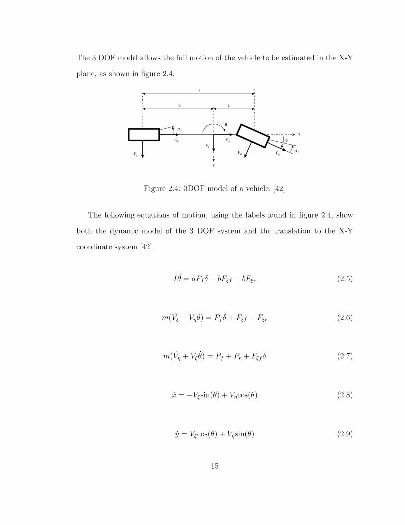
The 3 DOF model allows the full motion of the vehicle to be estimated in the X-Y
plane, as shown in figure 2.4.
Figure 2.4: 3DOF model of a vehicle, [42]
The following equations of motion, using the labels found in figure 2.4, show
both the dynamic model of the 3 DOF system and the translation to the X-Y
coordinate system [42].
Iθ = aPfδ + bFξf − bFξr (2.5)
m(Vξ + Vηθ) = Pfδ + Fξf + Fξr (2.6)
m(Vη + Vξθ) = Pf + Pr + Fξfδ (2.7)
x = −Vξsin(θ) + Vηcos(θ) (2.8)
y = Vξcos(θ) + Vηsin(θ) (2.9)
15
Equations 2.5 to 2.7 describe the motion of the vehicle relative to its own
coordinate system. Equations 2.8 and 2.9 translate the vehicles motion onto a
global X-Y plane.
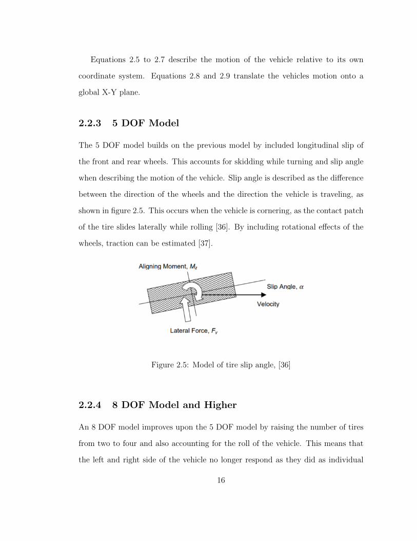
2.2.3 5 DOF Model
The 5 DOF model builds on the previous model by included longitudinal slip of
the front and rear wheels. This accounts for skidding while turning and slip angle
when describing the motion of the vehicle. Slip angle is described as the difference
between the direction of the wheels and the direction the vehicle is traveling, as
shown in figure 2.5. This occurs when the vehicle is cornering, as the contact patch
of the tire slides laterally while rolling [36]. By including rotational effects of the
wheels, traction can be estimated [37].
Figure 2.5: Model of tire slip angle, [36]
2.2.4 8 DOF Model and Higher
An 8 DOF model improves upon the 5 DOF model by raising the number of tires
from two to four and also accounting for the roll of the vehicle. This means that
the left and right side of the vehicle no longer respond as they did as individual
16
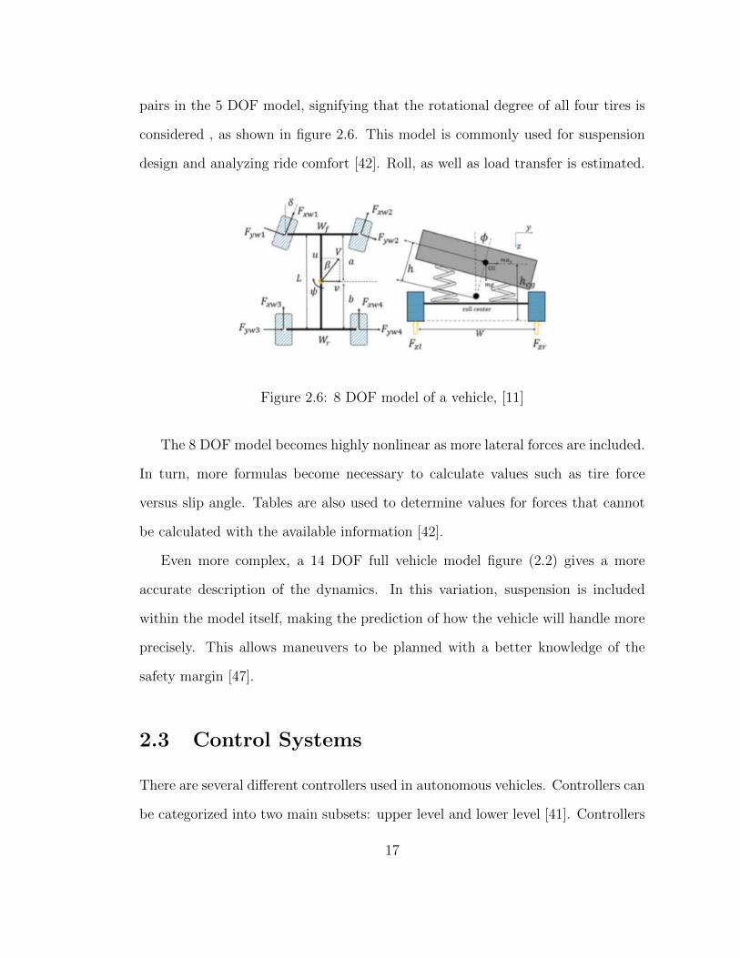
pairs in the 5 DOF model, signifying that the rotational degree of all four tires is
considered , as shown in figure 2.6. This model is commonly used for suspension
design and analyzing ride comfort [42]. Roll, as well as load transfer is estimated.
Figure 2.6: 8 DOF model of a vehicle, [11]
The 8 DOF model becomes highly nonlinear as more lateral forces are included.
In turn, more formulas become necessary to calculate values such as tire force
versus slip angle. Tables are also used to determine values for forces that cannot
be calculated with the available information [42].
Even more complex, a 14 DOF full vehicle model figure (2.2) gives a more
accurate description of the dynamics. In this variation, suspension is included
within the model itself, making the prediction of how the vehicle will handle more
precisely. This allows maneuvers to be planned with a better knowledge of the
safety margin [47].
2.3 Control Systems
There are several different controllers used in autonomous vehicles. Controllers can
be categorized into two main subsets: upper level and lower level [41]. Controllers
17
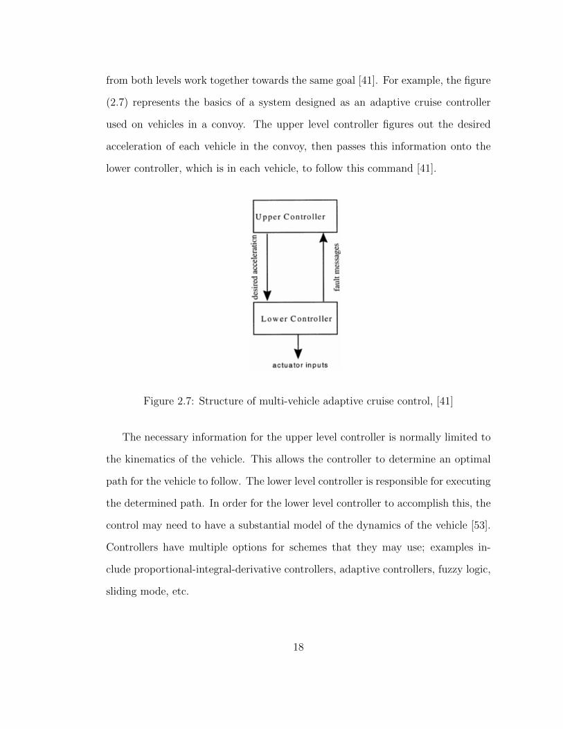
from both levels work together towards the same goal [41]. For example, the figure
(2.7) represents the basics of a system designed as an adaptive cruise controller
used on vehicles in a convoy. The upper level controller figures out the desired
acceleration of each vehicle in the convoy, then passes this information onto the
lower controller, which is in each vehicle, to follow this command [41].
Figure 2.7: Structure of multi-vehicle adaptive cruise control, [41]
The necessary information for the upper level controller is normally limited to
the kinematics of the vehicle. This allows the controller to determine an optimal
path for the vehicle to follow. The lower level controller is responsible for executing
the determined path. In order for the lower level controller to accomplish this, the
control may need to have a substantial model of the dynamics of the vehicle [53].
Controllers have multiple options for schemes that they may use; examples in-
clude proportional-integral-derivative controllers, adaptive controllers, fuzzy logic,
sliding mode, etc.
18
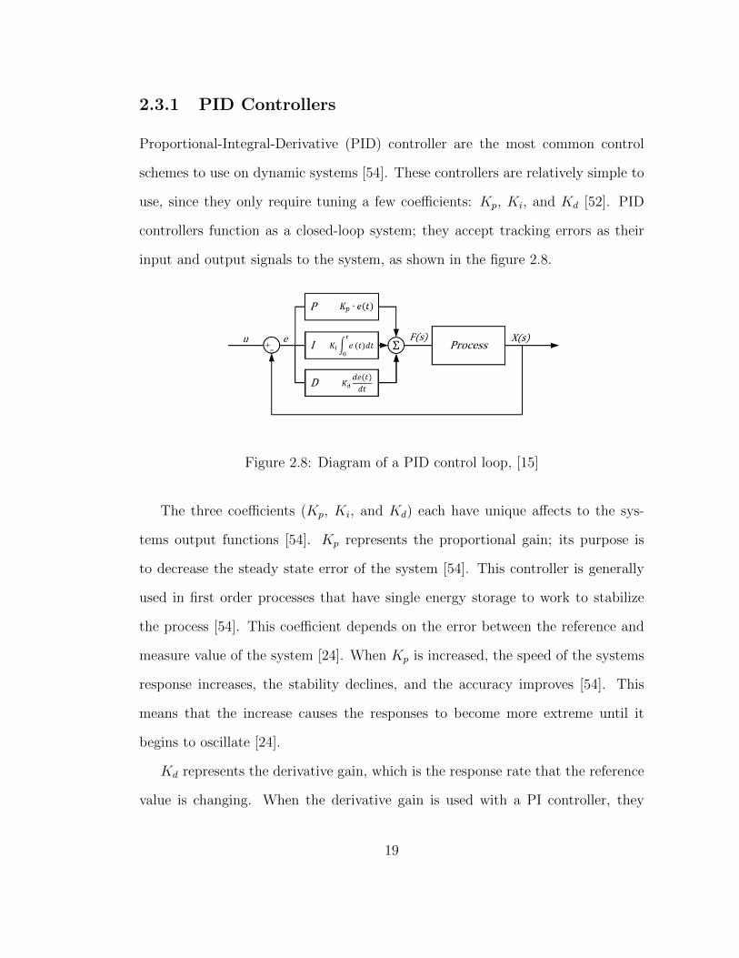
2.3.1 PID Controllers
Proportional-Integral-Derivative (PID) controller are the most common control
schemes to use on dynamic systems [54]. These controllers are relatively simple to
use, since they only require tuning a few coefficients: Kp, Ki, and Kd [52]. PID
controllers function as a closed-loop system; they accept tracking errors as their
input and output signals to the system, as shown in the figure 2.8.
Figure 2.8: Diagram of a PID control loop, [15]
The three coefficients (Kp, Ki, and Kd) each have unique affects to the sys-
tems output functions [54]. Kp represents the proportional gain; its purpose is
to decrease the steady state error of the system [54]. This controller is generally
used in first order processes that have single energy storage to work to stabilize
the process [54]. This coefficient depends on the error between the reference and
measure value of the system [24]. When Kp is increased, the speed of the systems
response increases, the stability declines, and the accuracy improves [54]. This
means that the increase causes the responses to become more extreme until it
begins to oscillate [24].
Kd represents the derivative gain, which is the response rate that the reference
value is changing. When the derivative gain is used with a PI controller, they
19
work together to eliminate the overshoot and oscillations that occur in the output
response of the system [54].If Kd is increased, the speed of the systems response
increases, the stability would improve, and the accuracy would not be affected [54].
Finally, Ki represents the integral component that aims to bring the steady
state error to zero [24]. If Ki were to increase, then the speed of the systems
response decreases, the stability declines, and the accuracy improves [54].
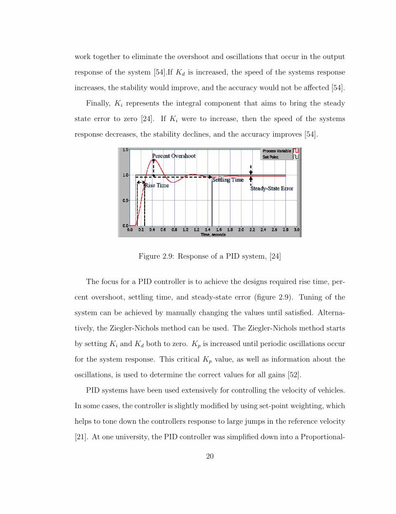
Figure 2.9: Response of a PID system, [24]
The focus for a PID controller is to achieve the designs required rise time, per-
cent overshoot, settling time, and steady-state error (figure 2.9). Tuning of the
system can be achieved by manually changing the values until satisfied. Alterna-
tively, the Ziegler-Nichols method can be used. The Ziegler-Nichols method starts
by setting Ki and Kd both to zero. Kp is increased until periodic oscillations occur
for the system response. This critical Kp value, as well as information about the
oscillations, is used to determine the correct values for all gains [52].
PID systems have been used extensively for controlling the velocity of vehicles.
In some cases, the controller is slightly modified by using set-point weighting, which
helps to tone down the controllers response to large jumps in the reference velocity
[21]. At one university, the PID controller was simplified down into a Proportional-
20
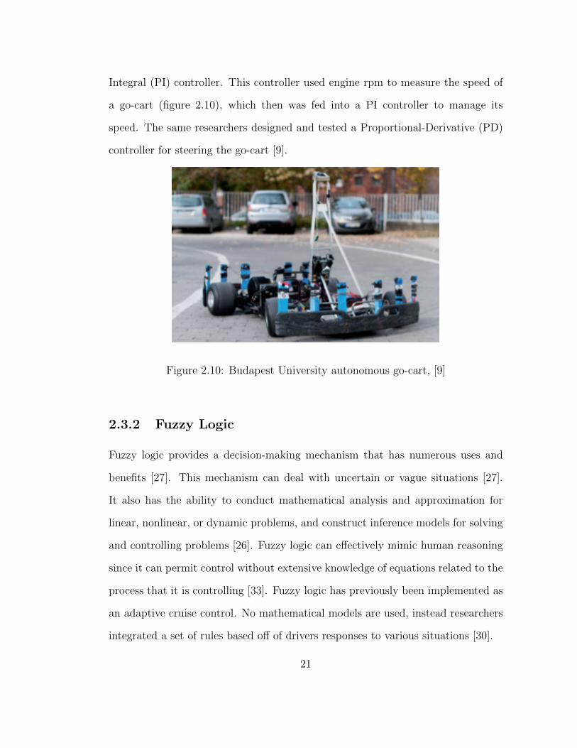
Integral (PI) controller. This controller used engine rpm to measure the speed of
a go-cart (figure 2.10), which then was fed into a PI controller to manage its
speed. The same researchers designed and tested a Proportional-Derivative (PD)
controller for steering the go-cart [9].
Figure 2.10: Budapest University autonomous go-cart, [9]
2.3.2 Fuzzy Logic
Fuzzy logic provides a decision-making mechanism that has numerous uses and
benefits [27]. This mechanism can deal with uncertain or vague situations [27].
It also has the ability to conduct mathematical analysis and approximation for
linear, nonlinear, or dynamic problems, and construct inference models for solving
and controlling problems [26]. Fuzzy logic can effectively mimic human reasoning
since it can permit control without extensive knowledge of equations related to the
process that it is controlling [33]. Fuzzy logic has previously been implemented as
an adaptive cruise control. No mathematical models are used, instead researchers
integrated a set of rules based off of drivers responses to various situations [30].
21
Fuzzy logic is dictated by a set of rules. These rules determine the responses
of the controller to the inputted information [33]. Information about the system is
initially passed through a filter that fuzzifies the information into values ranging
between 0 (false) and 1 (true) [46]. The fuzzified information is checked against the
rules, an output is determined, and then the output goes through a process called
deffuzification [46]. Using the previously mentioned fuzzy adaptive cruise control,
simple logic such as if the speed error is greater than 0 then decrease accelerator
input [31]. Once the input direction is determined, a simple equation (eqn 2.10)
calculates the proportion by which the accelerator changes [33].
xout =.33up+ .76down
.33 + .76(2.10)
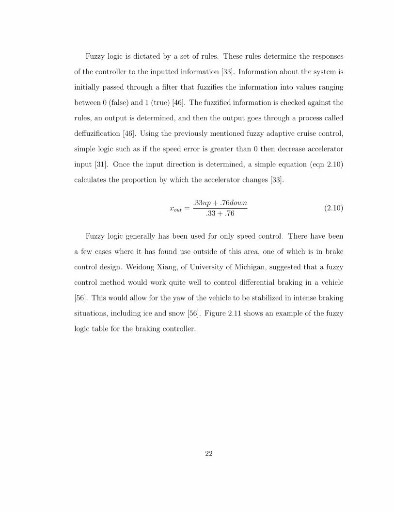
Fuzzy logic generally has been used for only speed control. There have been
a few cases where it has found use outside of this area, one of which is in brake
control design. Weidong Xiang, of University of Michigan, suggested that a fuzzy
control method would work quite well to control differential braking in a vehicle
[56]. This would allow for the yaw of the vehicle to be stabilized in intense braking
situations, including ice and snow [56]. Figure 2.11 shows an example of the fuzzy
logic table for the braking controller.
22
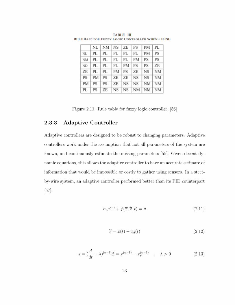
Figure 2.11: Rule table for fuzzy logic controller, [56]
2.3.3 Adaptive Controller
Adaptive controllers are designed to be robust to changing parameters. Adaptive
controllers work under the assumption that not all parameters of the system are
known, and continuously estimate the missing parameters [55]. Given decent dy-
namic equations, this allows the adaptive controller to have an accurate estimate of
information that would be impossible or costly to gather using sensors. In a steer-
by-wire system, an adaptive controller performed better than its PID counterpart
[57].
αox(n) + f(x, x, t) = u (2.11)
x = x(t)− xd(t) (2.12)
s = (d
dt+ λ)(n−1)x = x(n−1) − x(n−1)
r ; λ > 0 (2.13)
23
x(n−1)r = x
(n−1)d − (n− 1)λx(n−2) − ...− λ(n−1)x (2.14)
V =1
2αos
2 (2.15)
V = αoss = s(u− Y α) (2.16)
Y =
[Y0 Y1 ... Ym
](2.17)
α =
⎡⎢⎢⎢⎢⎢⎢⎢⎣
α0
α1
...
αm
⎤⎥⎥⎥⎥⎥⎥⎥⎦(2.18)
Equations 2.11 through 2.20 represent a generalized setup of an adaptive control
solution [49]. Given an equation with several unknown parameters (Equation 2.11),
the tracking error is brought into state space using Equation 2.13. The Lyapunov
function candidate is described with Equation 2.15 and then its derivative is taken.
The derivative is then used to come up with an input (Equation 2.19). The input,
u, makes use of the known parameters, Y, and the unknown estimated parameters,
α. The unknown estimated parameters are altered each iteration of the control
loop using Equation 2.20 [49].
u = Y α− ks ; k > 0 (2.19)
24
˙α = −PY T s ; P = P T > 0 (2.20)
2.3.4 Sliding Mode Controller
Sliding mode controllers have a variety of uses in autonomous vehicles. One ex-
ample is a Mixed Slip-Deceleration (MSD) controller designed by Mara Tanelli
that uses the sliding mode controller for braking [50]. Sliding mode controllers are
designed to take the system state into a region where s (the tracking error as a
sliding variable) is 0 . This brings the tracking error to zero as well when sliding
conditions are met [14].
x(n) = f(x, x, t) + u (2.21)
x = x− xd (2.22)
s = (d
dt+ λ)(n−1)x ; λ > 0 (2.23)
s = x(n) + λx(n−1) (2.24)
s = f(x, x, t) + u− x(n)d + λx(n−1) (2.25)
Equations 2.21 through 2.25 show the generalized setup for a sliding mode
controller [49]. The tracking error (2.22) is brought into a sliding plane using
Equation 2.23. From here, the derivative of s is taken, and then Equation 2.21 is
25
substituted inside Equation 2.24 to achieve Equation 2.25. This equation is then
rearranged to provide a preliminary input, u (Equation 2.26) [49].
Figure 2.12: Difference between Sign and Sat function, [14]
u = −f + x(n)d − λx(n−1) (2.26)
u = u− ksgn(s) (2.27)
u = u− (k − ϕ)sat(s
ϕ) (2.28)
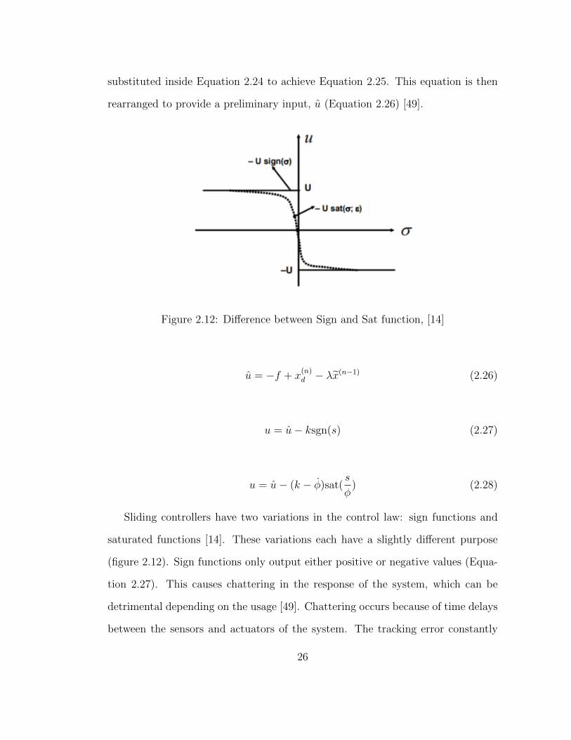
Sliding controllers have two variations in the control law: sign functions and
saturated functions [14]. These variations each have a slightly different purpose
(figure 2.12). Sign functions only output either positive or negative values (Equa-
tion 2.27). This causes chattering in the response of the system, which can be
detrimental depending on the usage [49]. Chattering occurs because of time delays
between the sensors and actuators of the system. The tracking error constantly
26
passes 0 and does not settle in most cases [49]. A saturation function stops the
chattering, but is at the cost of always leaving a slight tracking error in place
(Equation 2.28). In a lot of cases, the slight error is better than the possibility of
chattering [7].
2.4 ROS
The Robot Operating System, ROS, is an open source framework designed for
writing robot software [39]. This system is also a collection of libraries, tools and
conventions that help to simplify the task of implementing complex and dynamic
robot behavior across a broad range of robotic platforms [39]. The ideas for ROS
were initially developed by researchers at Stanford in 2007 [45]. From the time of
ROSs inception, it has grown extremely fast with the help of numerous contributors
[45]. The core features of ROS include communications and hardware integration.
2.4.1 Communication Framework
When a new robot application is being implemented, one of the first developments
needs to be a communication system [44]. ROS offers many options for passing
information to and from systems; these options are called nodes [44]. Each node
has its own separate task and they are available on any operating system. At
its most basic level, ROS acts as middleware. Middleware is a message passing
interface that allows for inter-process communication [44]. In the application to-
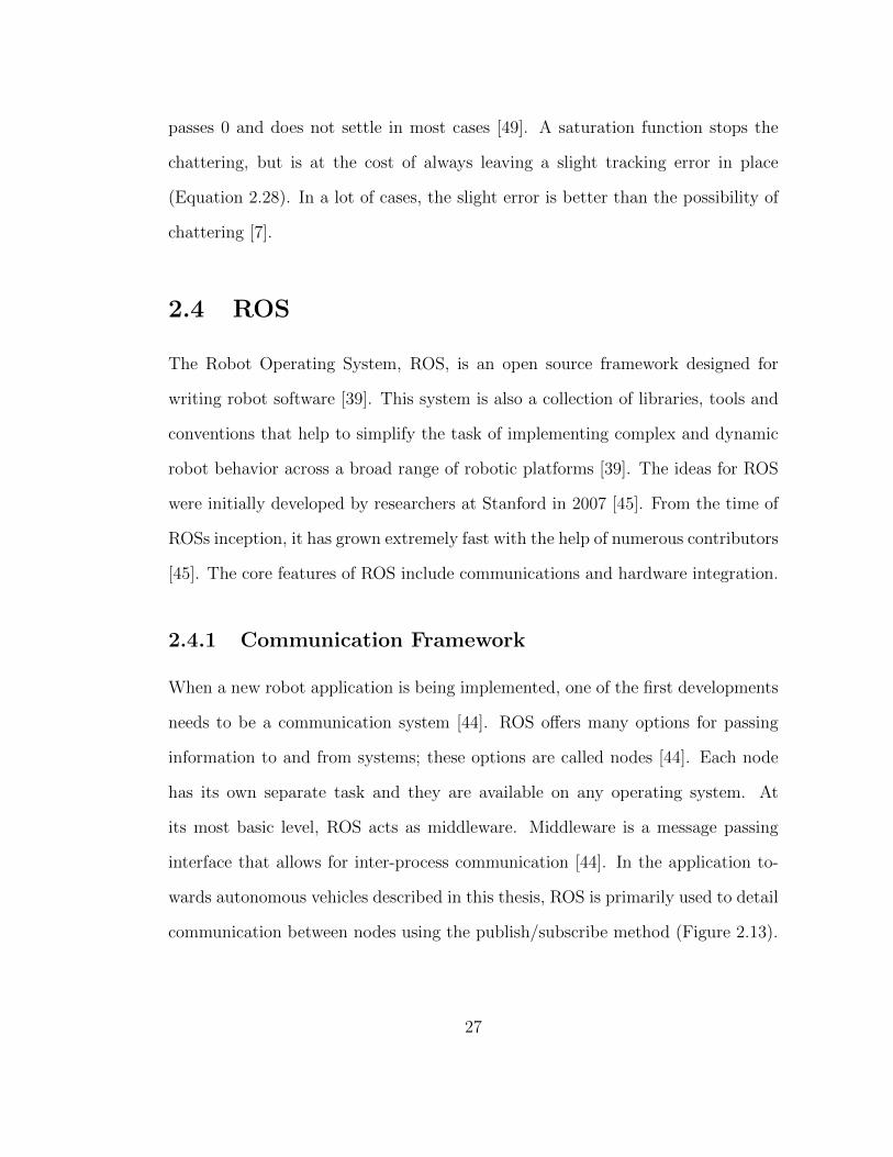
wards autonomous vehicles described in this thesis, ROS is primarily used to detail
communication between nodes using the publish/subscribe method (Figure 2.13).
27
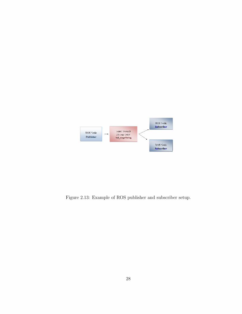
Figure 2.13: Example of ROS publisher and subscriber setup.
28
Chapter 3
Methodology
3.1 Overview of Polaris GEM e2
Figure 3.1: Polaris GEM e2, [38]
The Polaris Gem e2 is an electric powered FMVSS 500 class vehicle capable
of speeds up to 25 mph. It is front wheel drive and powered by an AC induction
motor. Braking is provided by disks on the front tires and hydraulic drums on
29
the rear tires. Information for the vehicle is provided via the data sheets from the
company [38].
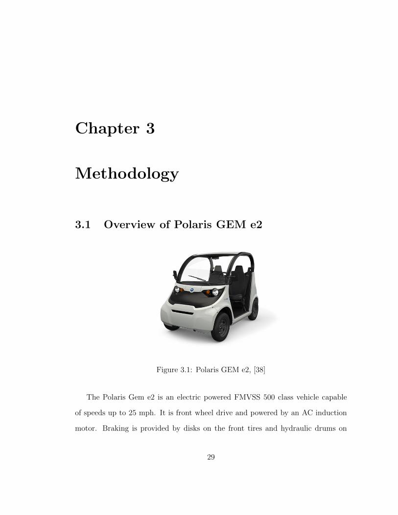
Table 3.1: Polaris GEM e2 Specifications [38]
Specification Imperial Values Metric Values
Top speed 25 mph 11.7 m/sEngine size 6.7 hp 5 kW h
Vehicle weight 1200 lbs 544 kgPayload 800 lbs 363 kg
Turning radius 150 in 3.81 mWheelbase 69 in 1.753 mBatteries 48 v 48 v
Dimensions(Lxwxh) 103x55.5x73 (in) 2.62x1.41x1.854 (m)Range 30 miles 48.2 km
3.2 Control Systems Overview
The project was divided into two main components: an upper level controller
and multiple lower level controllers, as shown in Figure 3.2. The upper level
controller determines the actions the vehicle should take to maintain a constant
velocity, accelerate, decelerate, or turn. It calculates a steering angle, as well as
the percentage the gas pedal and brake pedal should be applied. The upper level
controller then passes the desired values to three separate lower level controllers.
The lower level controllers use a combination of hardware and software to physically
generate the requested inputs. If any error or discrepancy occurs, the lower level
controller sends a fault message to alert the upper level controller of the situation.
30
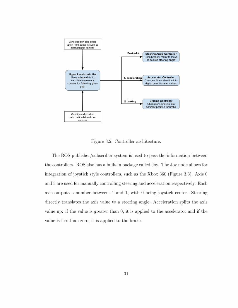
Figure 3.2: Controller architecture.
The ROS publisher/subscriber system is used to pass the information between
the controllers. ROS also has a built-in package called Joy. The Joy node allows for
integration of joystick style controllers, such as the Xbox 360 (Figure 3.3). Axis 0
and 3 are used for manually controlling steering and acceleration respectively. Each
axis outputs a number between -1 and 1, with 0 being joystick center. Steering
directly translates the axis value to a steering angle. Acceleration splits the axis
value up: if the value is greater than 0, it is applied to the accelerator and if the
value is less than zero, it is applied to the brake.
31
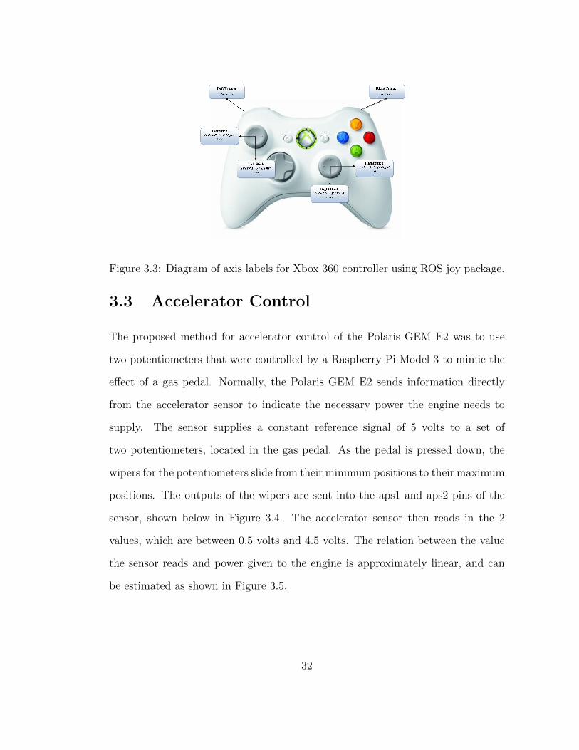
Figure 3.3: Diagram of axis labels for Xbox 360 controller using ROS joy package.
3.3 Accelerator Control
The proposed method for accelerator control of the Polaris GEM E2 was to use
two potentiometers that were controlled by a Raspberry Pi Model 3 to mimic the
effect of a gas pedal. Normally, the Polaris GEM E2 sends information directly
from the accelerator sensor to indicate the necessary power the engine needs to
supply. The sensor supplies a constant reference signal of 5 volts to a set of
two potentiometers, located in the gas pedal. As the pedal is pressed down, the
wipers for the potentiometers slide from their minimum positions to their maximum
positions. The outputs of the wipers are sent into the aps1 and aps2 pins of the
sensor, shown below in Figure 3.4. The accelerator sensor then reads in the 2
values, which are between 0.5 volts and 4.5 volts. The relation between the value
the sensor reads and power given to the engine is approximately linear, and can
be estimated as shown in Figure 3.5.
32
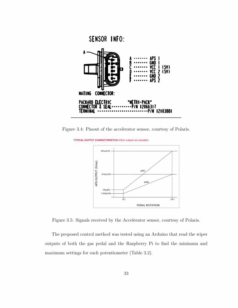
Figure 3.4: Pinout of the accelerator sensor, courtesy of Polaris.
Figure 3.5: Signals received by the Accelerator sensor, courtesy of Polaris.
The proposed control method was tested using an Arduino that read the wiper
outputs of both the gas pedal and the Raspberry Pi to find the minimum and
maximum settings for each potentiometer (Table 3.2).
33
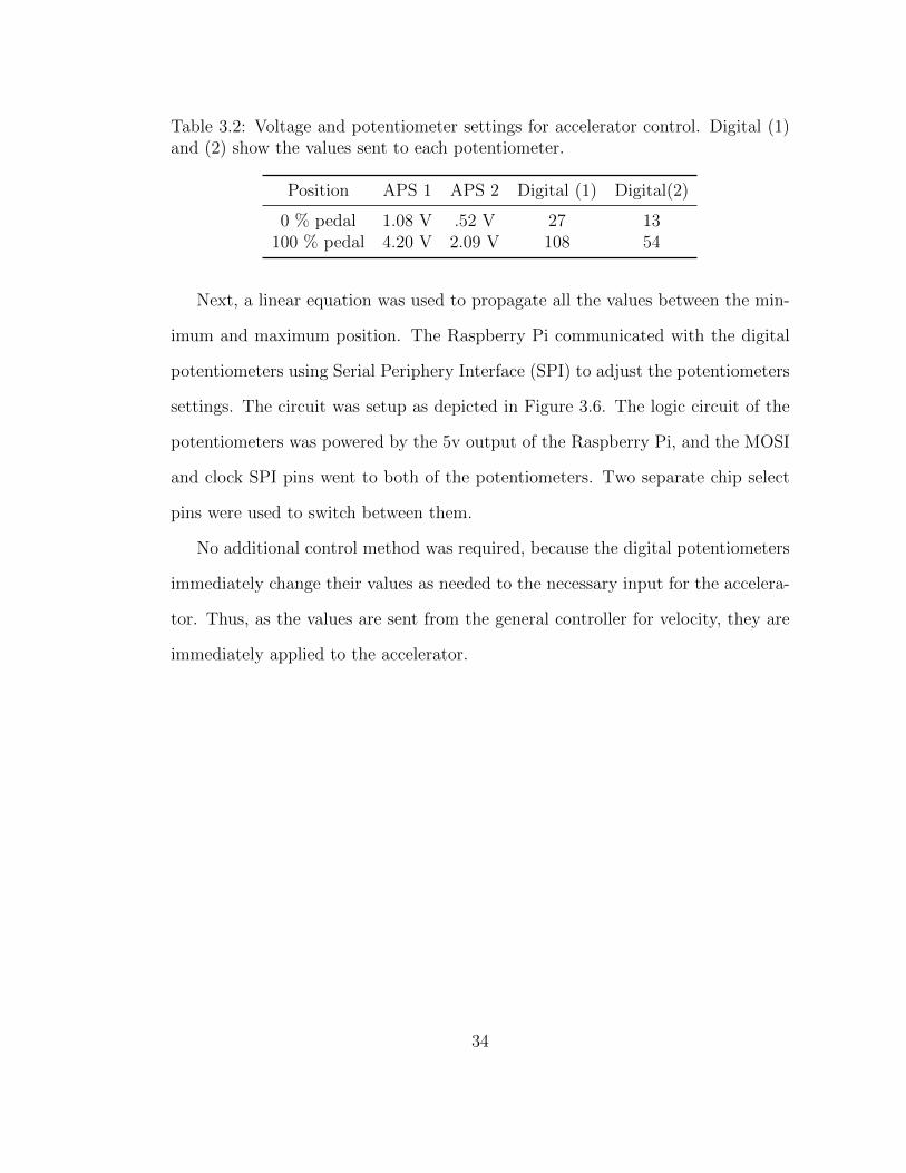
Table 3.2: Voltage and potentiometer settings for accelerator control. Digital (1)and (2) show the values sent to each potentiometer.
Position APS 1 APS 2 Digital (1) Digital(2)
0 % pedal 1.08 V .52 V 27 13100 % pedal 4.20 V 2.09 V 108 54
Next, a linear equation was used to propagate all the values between the min-
imum and maximum position. The Raspberry Pi communicated with the digital
potentiometers using Serial Periphery Interface (SPI) to adjust the potentiometers
settings. The circuit was setup as depicted in Figure 3.6. The logic circuit of the
potentiometers was powered by the 5v output of the Raspberry Pi, and the MOSI
and clock SPI pins went to both of the potentiometers. Two separate chip select
pins were used to switch between them.
No additional control method was required, because the digital potentiometers
immediately change their values as needed to the necessary input for the accelera-
tor. Thus, as the values are sent from the general controller for velocity, they are
immediately applied to the accelerator.
34
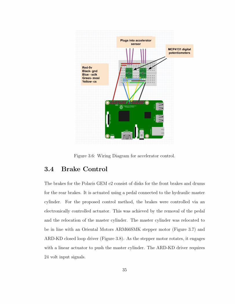
Figure 3.6: Wiring Diagram for accelerator control.
3.4 Brake Control
The brakes for the Polaris GEM e2 consist of disks for the front brakes and drums
for the rear brakes. It is actuated using a pedal connected to the hydraulic master
cylinder. For the proposed control method, the brakes were controlled via an
electronically controlled actuator. This was achieved by the removal of the pedal
and the relocation of the master cylinder. The master cylinder was relocated to
be in line with an Oriental Motors ARM66SMK stepper motor (Figure 3.7) and
ARD-KD closed loop driver (Figure 3.8). As the stepper motor rotates, it engages
with a linear actuator to push the master cylinder. The ARD-KD driver requires
24 volt input signals.
35
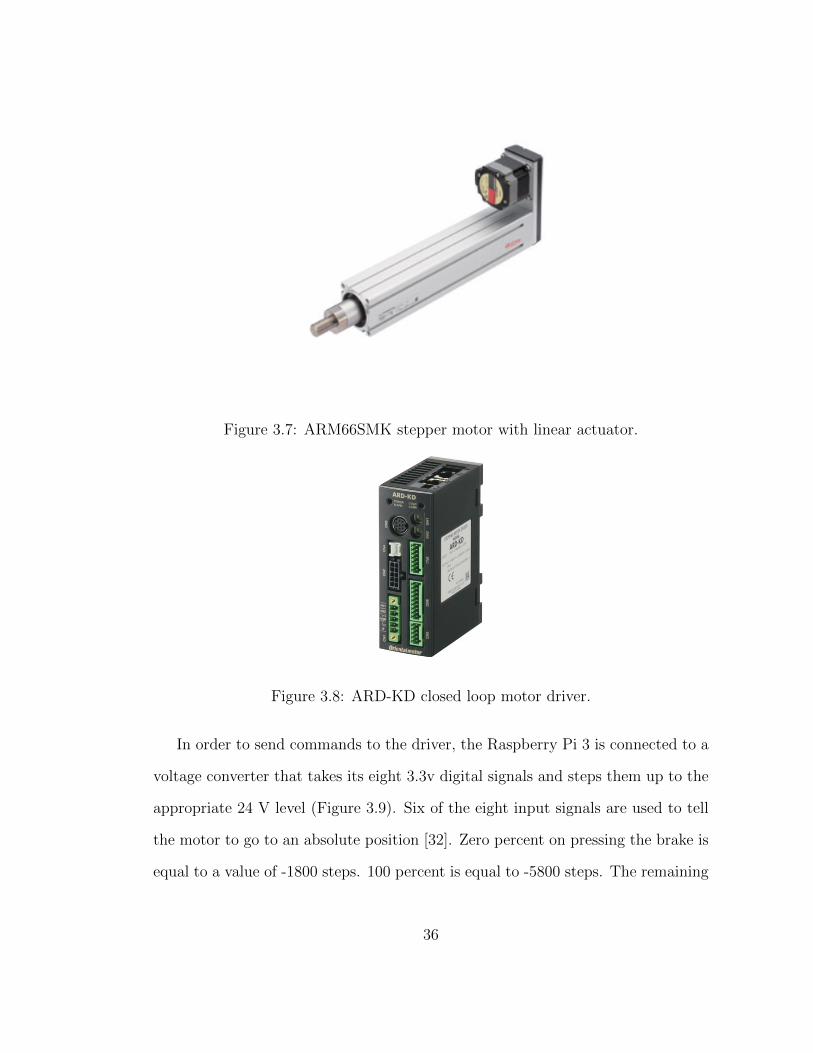
Figure 3.7: ARM66SMK stepper motor with linear actuator.
Figure 3.8: ARD-KD closed loop motor driver.
In order to send commands to the driver, the Raspberry Pi 3 is connected to a
voltage converter that takes its eight 3.3v digital signals and steps them up to the
appropriate 24 V level (Figure 3.9). Six of the eight input signals are used to tell
the motor to go to an absolute position [32]. Zero percent on pressing the brake is
equal to a value of -1800 steps. 100 percent is equal to -5800 steps. The remaining
36
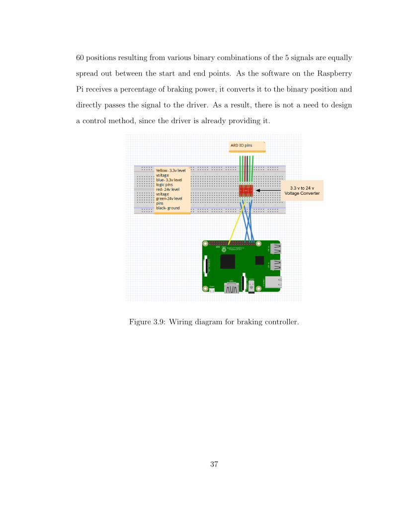
60 positions resulting from various binary combinations of the 5 signals are equally
spread out between the start and end points. As the software on the Raspberry
Pi receives a percentage of braking power, it converts it to the binary position and
directly passes the signal to the driver. As a result, there is not a need to design
a control method, since the driver is already providing it.
Figure 3.9: Wiring diagram for braking controller.
37
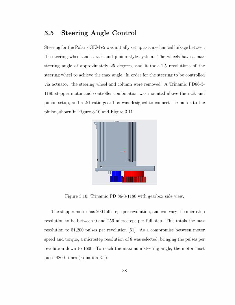
3.5 Steering Angle Control
Steering for the Polaris GEM e2 was initially set up as a mechanical linkage between
the steering wheel and a rack and pinion style system. The wheels have a max
steering angle of approximately 25 degrees, and it took 1.5 revolutions of the
steering wheel to achieve the max angle. In order for the steering to be controlled
via actuator, the steering wheel and column were removed. A Trinamic PD86-3-
1180 stepper motor and controller combination was mounted above the rack and
pinion setup, and a 2:1 ratio gear box was designed to connect the motor to the
pinion, shown in Figure 3.10 and Figure 3.11.
Figure 3.10: Trinamic PD 86-3-1180 with gearbox side view.
The stepper motor has 200 full steps per revolution, and can vary the microstep
resolution to be between 0 and 256 microsteps per full step. This totals the max
resolution to 51,200 pulses per revolution [51]. As a compromise between motor
speed and torque, a microstep resolution of 8 was selected, bringing the pulses per
revolution down to 1600. To reach the maximum steering angle, the motor must
pulse 4800 times (Equation 3.1).
38
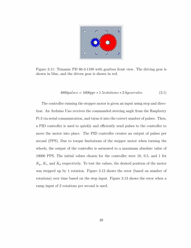
Figure 3.11: Trinamic PD 86-3-1180 with gearbox front view. The driving gear isshown in blue, and the driven gear is shown in red.
4800pulses = 1600ppr ∗ 1.5rotations ∗ 2.0gearratio (3.1)
The controller running the stepper motor is given an input using step and direc-
tion. An Arduino Uno receives the commanded steering angle from the Raspberry
Pi 3 via serial communication, and turns it into the correct number of pulses. Then,
a PID controller is used to quickly and efficiently send pulses to the controller to
move the motor into place. The PID controller creates an output of pulses per
second (PPS). Due to torque limitations of the stepper motor when turning the
wheels, the output of the controller is saturated to a maximum absolute value of
10000 PPS. The initial values chosen for the controller were 10, 0.5, and 1 for
Kp, Ki, and Kd respectively. To test the values, the desired position of the motor
was stepped up by 1 rotation. Figure 3.12 shows the error (based on number of
rotations) over time based on the step input. Figure 3.13 shows the error when a
ramp input of 2 rotations per second is used.
39
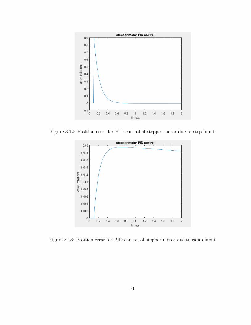
Figure 3.12: Position error for PID control of stepper motor due to step input.
Figure 3.13: Position error for PID control of stepper motor due to ramp input.
40
3.6 Kinematic Model for Simulations
To properly model the path for the vehicle, several factors had to be taken into
consideration. These included the speed that the vehicle would be allowed to
travel, the likelihood of wheel slip, and vehicle parameters such as minimum turn-
ing radius. A 2 degree-of-freedom model was selected based off of these criteria.
The diagram for the 2 DOF model can be found in Figure 2.3. The vehicle uses
an inputted speed and steering angle to calculate the body slip angle, rate of rota-
tion of the vehicle, and velocity in the X and Y direction, using slightly modified
equations from section 2.2.1:
X = V cos(ψ + β) (3.2)
Y = V sin(ψ + β) (3.3)
ψ =V sin(β)
ℓr(3.4)
β = arctan(tan(δf )ℓr
ℓf + ℓr) (3.5)
Generally, this model is good for lower speed applications, but starts deviating
from higher DOF models as the speed increases above a certain point due to tire
slip [21]. In order to consider the 2 DOF model an accurate representation, the
maximum lateral acceleration of the car had to stay under:
aymax = .5µg (3.6)
41
Generally for dry roads, µ= 0.7 is used [28]. This results in a maximum lat-
eral acceleration of 3.43 ms2. During the Self Drive Challenge that the vehicle will
participate in, the maximum allowed speed is 5 mph [23]. This converts to ap-
proximately 2.24 m/s. The minimum turning radius of the Polaris GEM e2 is 3.81
meters. When using the equation for centripetal acceleration:
ac =v2
R(3.7)
the maximum possible lateral acceleration under the given conditions was found
to be 1.32 ms2, which is well below where the limitations of the 2 DOF model begin
to show. Using the same minimum turn radius, the maximum speed that would
still allow the 2 DOF model to be valid is 3.62 m/s, or 8.1 mph. These equations
can also be used to figure out the minimum turning radius at any given speed for
the vehicle.
3.7 Dynamic Model for Longitudinal Motion
For the purposes of modelling speed, the vehicle was assumed to be moving in a
straight line. This limits velocity to a 1 DOF problem that can be used in addition
to the 2DOF model, giving a total of 3DOF. The assumption was made that the
wheels are solid disks with a moment of inertia:
I =1
2mr2 (3.8)
Since the vehicle does not has to perform high magnitude accelerations, the
tires would not be experiencing significant compression. Thus, solid disks were
42
chosen, so that the compression of the tires would be ignored for the derivation.
The wheels also operate without slip on the surface, which holds true as long as
the angular acceleration of each wheel does not override the force of friction. There
are two drag related forces acting on the vehicle against the direction of motion.
They are both functions of the vehicles geometry and speed. Aerodynamic drag
can be calculated with Equation 3.9. Rolling resistance, the other source of drag,
can be calculated with Equation 3.10. Combining the two forces results in the
total force from drag.
Fa =1
2CdρAx
2 (3.9)
Fr =MgCrx (3.10)
Fd = Fa + Fr (3.11)
The front wheels are given a driving torque, which can be broken down into
two separate sources of torque. Ta is the torque resulting from the acceleration
and deceleration of the engine. Tb is the torque resulting from the the cars brakes.
It was assumed positive torque will purely come from Ta and negative torque will
purely come from Tb. The braking torque has a simplified equation, Equation 3.14,
which allows it to convert the torque to a percentage of how far the brake is pressed
[48]. The engine torque was modeled as a linear function relating the amount the
gas pedal was pressed to the amount of torque delivered by the engine; this maxed
out at 1000 N-m.
T = Ta + Tb (3.12)
43
Ta = 1000ua (3.13)
Tb = 1.5ubKbmin(1,ω
α) (3.14)
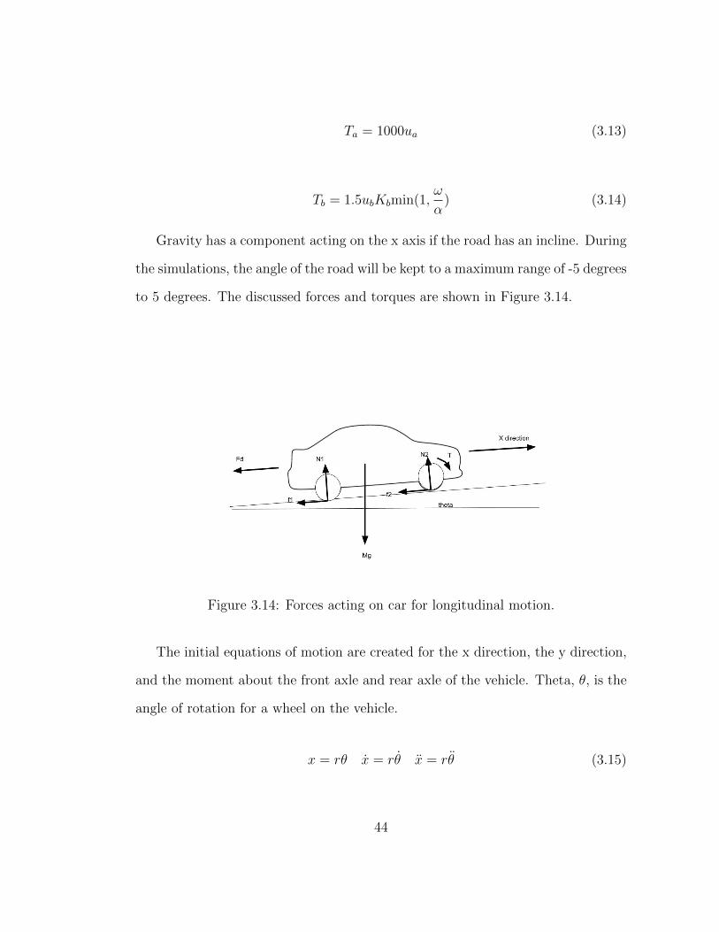
Gravity has a component acting on the x axis if the road has an incline. During
the simulations, the angle of the road will be kept to a maximum range of -5 degrees
to 5 degrees. The discussed forces and torques are shown in Figure 3.14.
Figure 3.14: Forces acting on car for longitudinal motion.
The initial equations of motion are created for the x direction, the y direction,
and the moment about the front axle and rear axle of the vehicle. Theta, θ, is the
angle of rotation for a wheel on the vehicle.
x = rθ x = rθ x = rθ (3.15)
44
x : −MgsinΘ− f1 − f2 −1
2CdρAx
2 −MgCrx =Mx (3.16)
y : N1 +N2 −MgcosΘ = 0 (3.17)
frontwheels : T + f1r =1
2mr2
x
r(3.18)
rearwheels : f2r =1
2mr2
x
r(3.19)
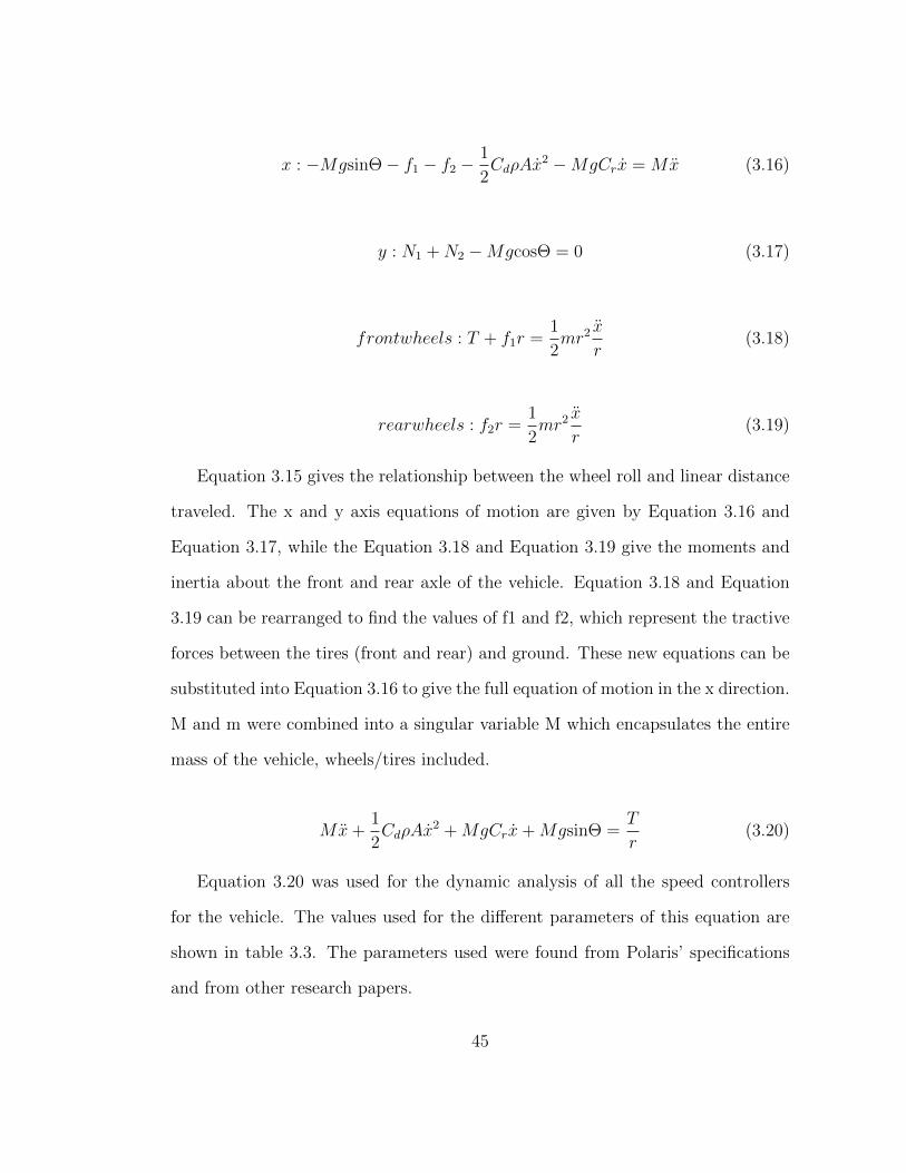
Equation 3.15 gives the relationship between the wheel roll and linear distance
traveled. The x and y axis equations of motion are given by Equation 3.16 and
Equation 3.17, while the Equation 3.18 and Equation 3.19 give the moments and
inertia about the front and rear axle of the vehicle. Equation 3.18 and Equation
3.19 can be rearranged to find the values of f1 and f2, which represent the tractive
forces between the tires (front and rear) and ground. These new equations can be
substituted into Equation 3.16 to give the full equation of motion in the x direction.
M and m were combined into a singular variable M which encapsulates the entire
mass of the vehicle, wheels/tires included.
Mx+1
2CdρAx
2 +MgCrx+MgsinΘ =T
r(3.20)
Equation 3.20 was used for the dynamic analysis of all the speed controllers
for the vehicle. The values used for the different parameters of this equation are
shown in table 3.3. The parameters used were found from Polaris’ specifications
and from other research papers.
45
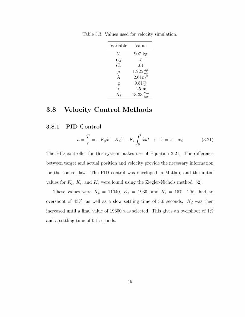
Table 3.3: Values used for velocity simulation.
Variable Value
M 907 kgCd .5Cr .01
ρ 1.225 kgm3
A 2.61m2
g 9.81ms2
r .25 mKb 13.33Nm
bar
3.8 Velocity Control Methods
3.8.1 PID Control
u =T
r= −Kpx−Kd
˙x−Ki
∫ t
0
xdt ; x = x− xd (3.21)
The PID controller for this system makes use of Equation 3.21. The difference
between target and actual position and velocity provide the necessary information
for the control law. The PID control was developed in Matlab, and the initial
values for Kp, Ki, and Kd were found using the Ziegler-Nichols method [52].
These values were Kp = 11040, Kd = 1930, and Ki = 157. This had an
overshoot of 43%, as well as a slow settling time of 3.6 seconds. Kd was then
increased until a final value of 19300 was selected. This gives an overshoot of 1%
and a settling time of 0.1 seconds.
46
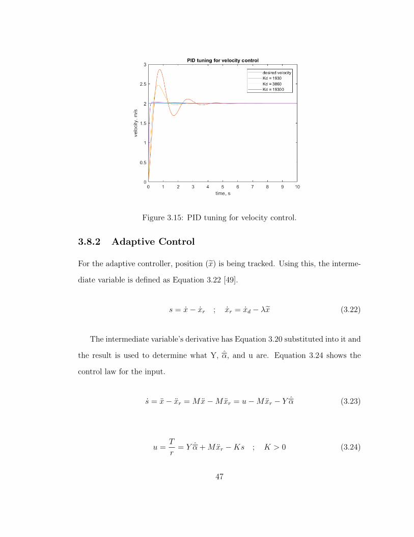
Figure 3.15: PID tuning for velocity control.
3.8.2 Adaptive Control
For the adaptive controller, position (x) is being tracked. Using this, the interme-
diate variable is defined as Equation 3.22 [49].
s = x− xr ; xr = xd − λx (3.22)
The intermediate variable’s derivative has Equation 3.20 substituted into it and
the result is used to determine what Y, α, and u are. Equation 3.24 shows the
control law for the input.
s = x− xr =Mx−Mxr = u−Mxr − Y α (3.23)
u =T
r= Y α +Mxr −Ks ; K > 0 (3.24)
47
˙α = −PY T s ; P = P T > 0 (3.25)
The controller can estimate what α is using Equation 3.25. For this controller,
it was decided that the incline, aerodynamic drag, and rolling resistance would all
be tracked. Y and α become:
Y =
[Mg .5x2 x
](3.26)
α =
⎡⎢⎢⎢⎢⎣sinΘ
CdρA
MgCr
⎤⎥⎥⎥⎥⎦ (3.27)
48
3.8.3 Simulated Paths
Multiple functions were desired for testing velocity control. For accelerating to
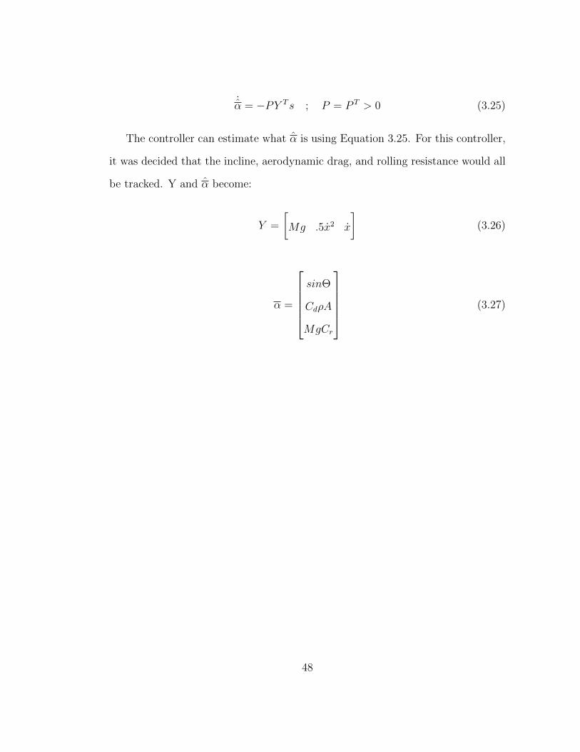
a set speed, the velocity should not have any sudden and drastic changes to it.
Therefore, a desired velocity of Equation 3.28 was used.
x = 2(1− e−.5t) (3.28)
Figure 3.16: Desired velocity of vehicle during acceleration simulation.
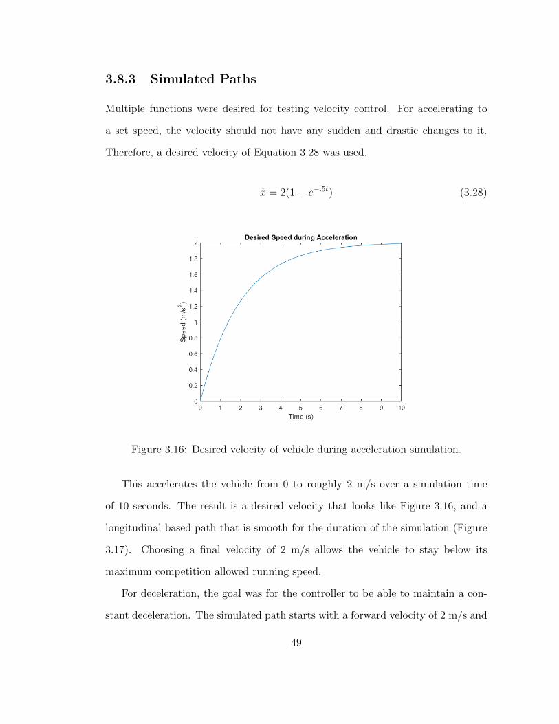
This accelerates the vehicle from 0 to roughly 2 m/s over a simulation time
of 10 seconds. The result is a desired velocity that looks like Figure 3.16, and a
longitudinal based path that is smooth for the duration of the simulation (Figure
3.17). Choosing a final velocity of 2 m/s allows the vehicle to stay below its
maximum competition allowed running speed.
For deceleration, the goal was for the controller to be able to maintain a con-
stant deceleration. The simulated path starts with a forward velocity of 2 m/s and
49
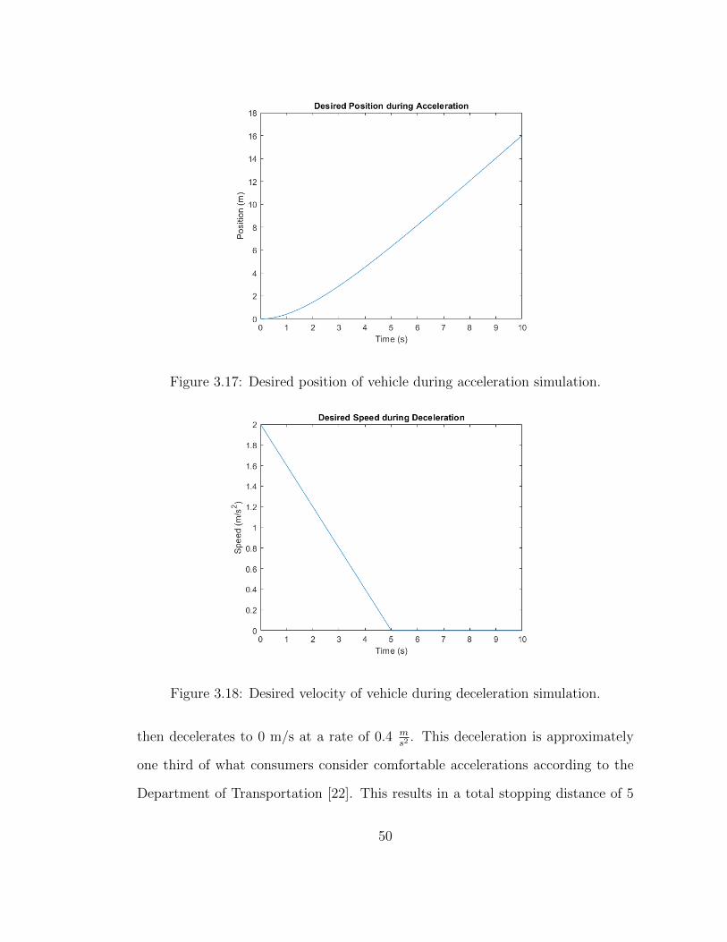
Figure 3.17: Desired position of vehicle during acceleration simulation.
Figure 3.18: Desired velocity of vehicle during deceleration simulation.
then decelerates to 0 m/s at a rate of 0.4 ms2. This deceleration is approximately
one third of what consumers consider comfortable accelerations according to the
Department of Transportation [22]. This results in a total stopping distance of 5
50
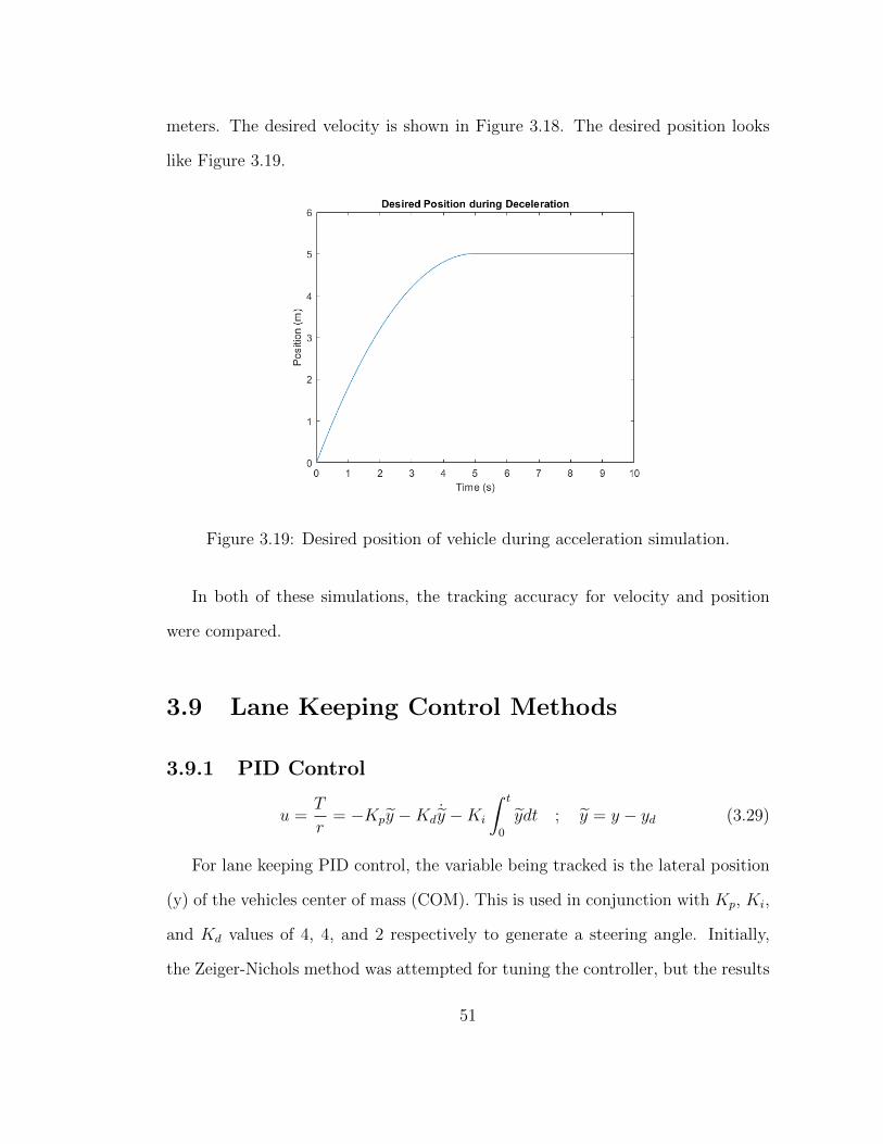
meters. The desired velocity is shown in Figure 3.18. The desired position looks
like Figure 3.19.
Figure 3.19: Desired position of vehicle during acceleration simulation.
In both of these simulations, the tracking accuracy for velocity and position
were compared.
3.9 Lane Keeping Control Methods
3.9.1 PID Control
u =T
r= −Kpy −Kd
˙y −Ki
∫ t
0
ydt ; y = y − yd (3.29)
For lane keeping PID control, the variable being tracked is the lateral position
(y) of the vehicles center of mass (COM). This is used in conjunction with Kp, Ki,
and Kd values of 4, 4, and 2 respectively to generate a steering angle. Initially,
the Zeiger-Nichols method was attempted for tuning the controller, but the results
51
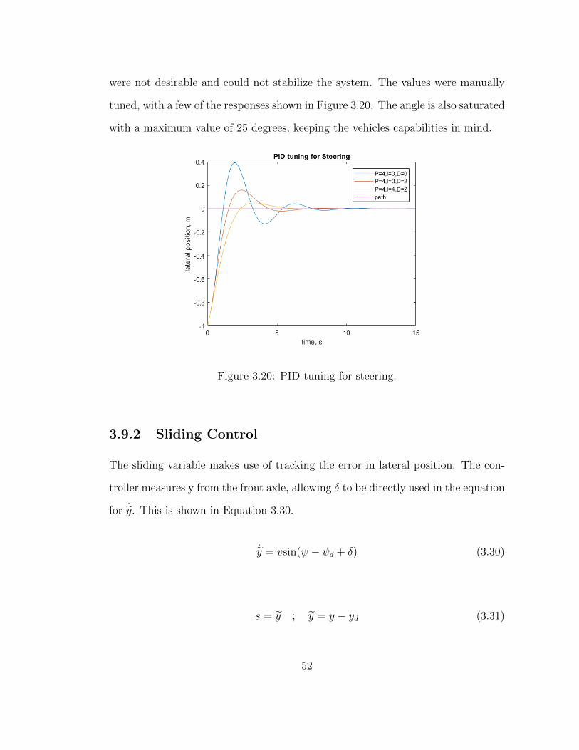
were not desirable and could not stabilize the system. The values were manually
tuned, with a few of the responses shown in Figure 3.20. The angle is also saturated
with a maximum value of 25 degrees, keeping the vehicles capabilities in mind.
Figure 3.20: PID tuning for steering.
3.9.2 Sliding Control
The sliding variable makes use of tracking the error in lateral position. The con-
troller measures y from the front axle, allowing δ to be directly used in the equation
for ˙y. This is shown in Equation 3.30.
˙y = vsin(ψ − ψd + δ) (3.30)
s = y ; y = y − yd (3.31)
52
s = ˙y (3.32)
δ = −(ψ − ψd) (3.33)
δ = δ +Ksat(s
ϕ) ; ϕ =
K
λ(3.34)
The derivative of the sliding variable has Equation 3.30 substituted into it. It
is then inverted to get an initial input, δ, which keeps the sliding plane s at zero.
In order to bring initial non-zero values onto the sliding plane, a reaching condition
is added. Initially, a sign function was used, but it resulted in chattering of the
lateral position. The sign function was changed to the saturation function, shown
in Equation 3.34. After manually testing, values for K and λ were found to be 12
and 25 respectively.
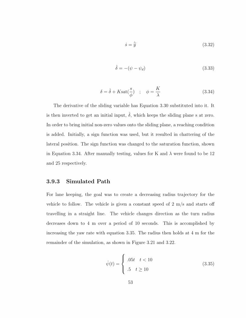
3.9.3 Simulated Path
For lane keeping, the goal was to create a decreasing radius trajectory for the
vehicle to follow. The vehicle is given a constant speed of 2 m/s and starts off
travelling in a straight line. The vehicle changes direction as the turn radius
decreases down to 4 m over a period of 10 seconds. This is accomplished by
increasing the yaw rate with equation 3.35. The radius then holds at 4 m for the
remainder of the simulation, as shown in Figure 3.21 and 3.22.
ψ(t) =
⎧⎪⎨⎪⎩ .05t t < 10
.5 t ≥ 10(3.35)
53
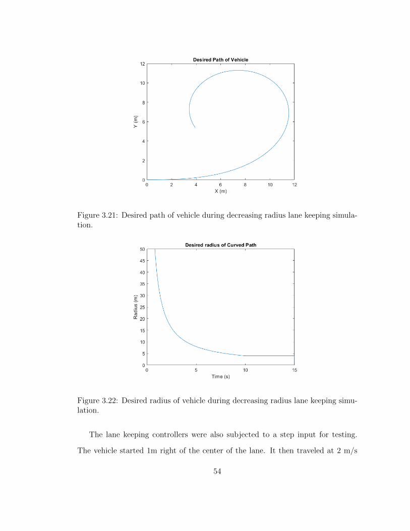
Figure 3.21: Desired path of vehicle during decreasing radius lane keeping simula-tion.
Figure 3.22: Desired radius of vehicle during decreasing radius lane keeping simu-lation.
The lane keeping controllers were also subjected to a step input for testing.
The vehicle started 1m right of the center of the lane. It then traveled at 2 m/s
54
and attempted to center itself in the lane using the different control methods.
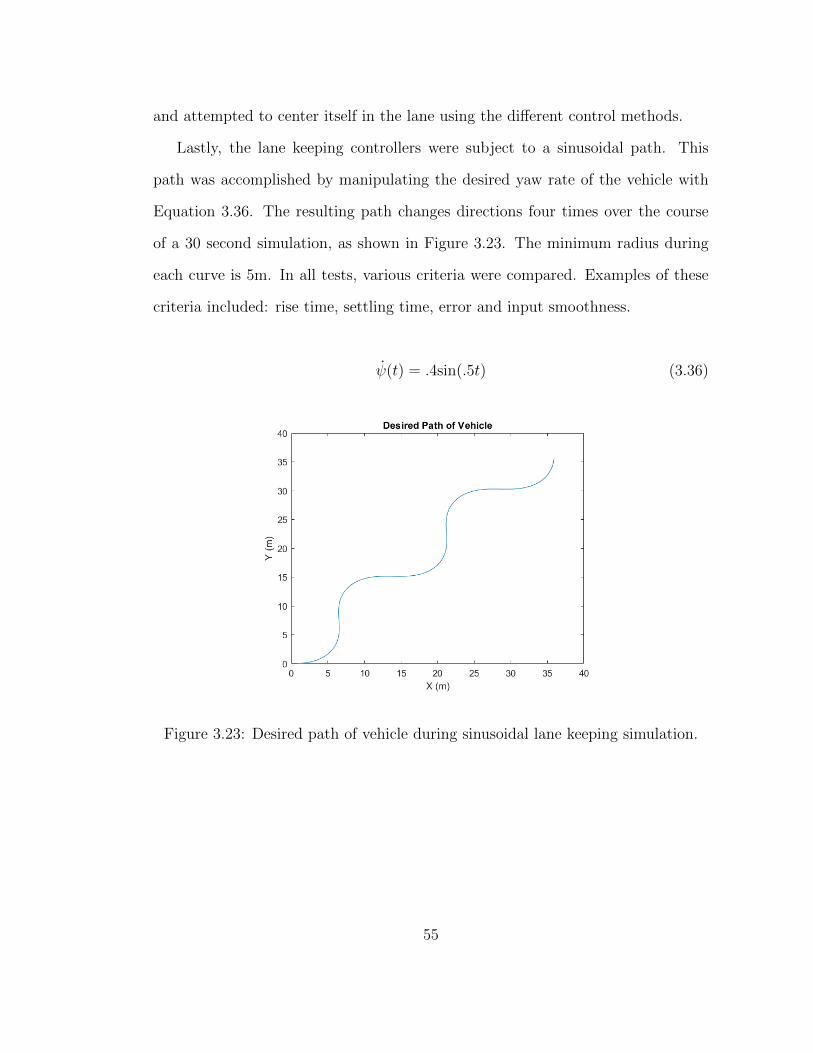
Lastly, the lane keeping controllers were subject to a sinusoidal path. This
path was accomplished by manipulating the desired yaw rate of the vehicle with
Equation 3.36. The resulting path changes directions four times over the course
of a 30 second simulation, as shown in Figure 3.23. The minimum radius during
each curve is 5m. In all tests, various criteria were compared. Examples of these
criteria included: rise time, settling time, error and input smoothness.
ψ(t) = .4sin(.5t) (3.36)
Figure 3.23: Desired path of vehicle during sinusoidal lane keeping simulation.
55
Chapter 4
Results
4.1 Velocity Control
4.1.1 Acceleration
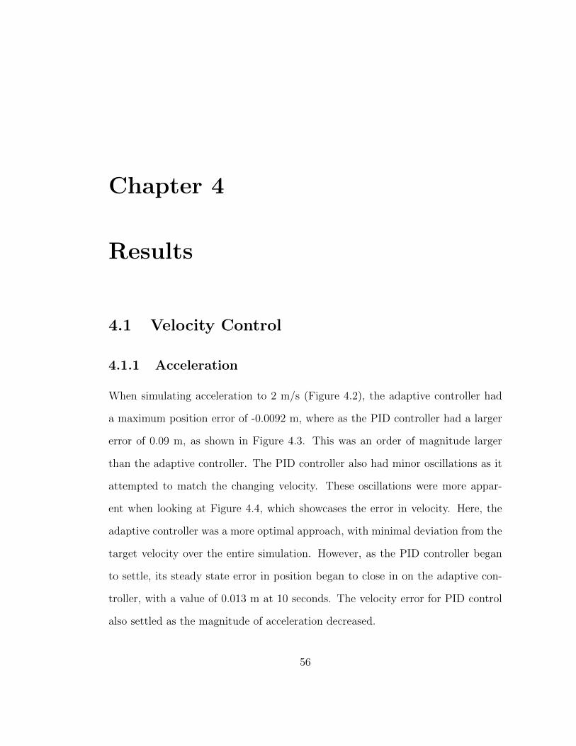
When simulating acceleration to 2 m/s (Figure 4.2), the adaptive controller had
a maximum position error of -0.0092 m, where as the PID controller had a larger
error of 0.09 m, as shown in Figure 4.3. This was an order of magnitude larger
than the adaptive controller. The PID controller also had minor oscillations as it
attempted to match the changing velocity. These oscillations were more appar-
ent when looking at Figure 4.4, which showcases the error in velocity. Here, the
adaptive controller was a more optimal approach, with minimal deviation from the
target velocity over the entire simulation. However, as the PID controller began
to settle, its steady state error in position began to close in on the adaptive con-
troller, with a value of 0.013 m at 10 seconds. The velocity error for PID control
also settled as the magnitude of acceleration decreased.
56
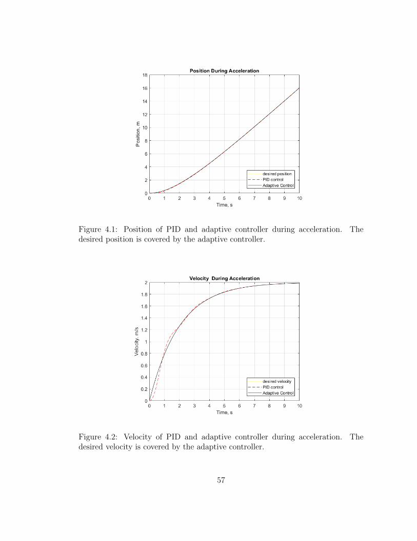
Figure 4.1: Position of PID and adaptive controller during acceleration. Thedesired position is covered by the adaptive controller.
Figure 4.2: Velocity of PID and adaptive controller during acceleration. Thedesired velocity is covered by the adaptive controller.
57
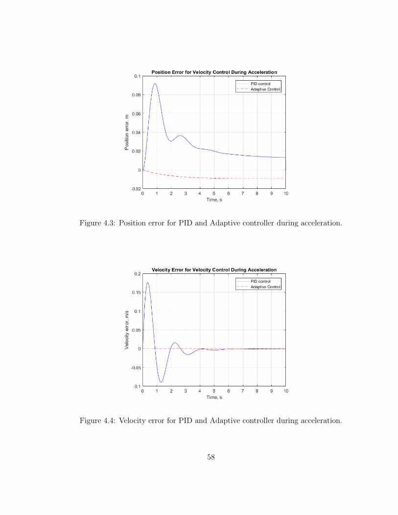
Figure 4.3: Position error for PID and Adaptive controller during acceleration.
Figure 4.4: Velocity error for PID and Adaptive controller during acceleration.
58
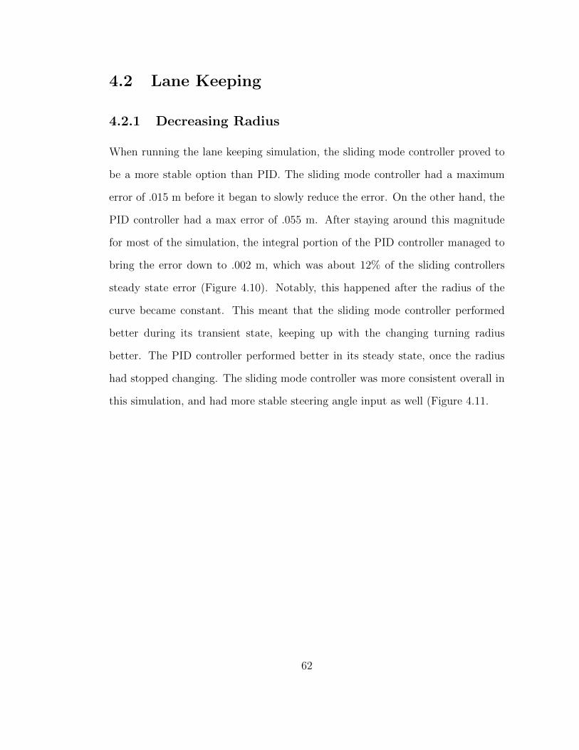
4.1.2 Deceleration
The adaptive controller tended to show a negative error throughout testing, this
was exacerbated during deceleration tests as shown by the velocity error in Figure
4.8. This meant that the adaptive controller had tendencies to err on the side of
being faster than the desired velocity, albeit by a very small amount (less than .01
m/s). Once again, the PID controller had diminishing oscillations in its velocity.
As with accelerating, this caused more initial variation in the error. The adaptive
controller ended up with a maximum error of -0.023 m, and the PID controller
ended with a -0.031 m error, as seen in Figure 4.7. Neither of the controllers were
allowed to have a negative velocity during simulation, because it was assumed
the vehicle would not shift from drive to reverse to fix any position error once it
stopped moving. This meant the position error remained the same once velocity
reached zero. Also, both velocity errors also jump to zero at approximately 5
seconds since the software prohibited the controllers from reversing the vehicle’s
direction. While the PID controller had a larger error in position, its steady state
error in velocity ended up being 75% of the adaptive controllers steady state error
(not including both the controller’s holding at 0 m/s once they stopped).
59
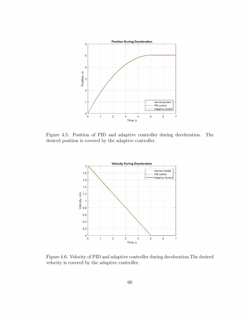
Figure 4.5: Position of PID and adaptive controller during deceleration. Thedesired position is covered by the adaptive controller.
Figure 4.6: Velocity of PID and adaptive controller during deceleration.The desiredvelocity is covered by the adaptive controller.
60
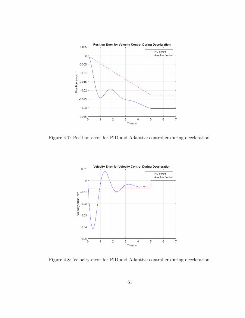
Figure 4.7: Position error for PID and Adaptive controller during deceleration.
Figure 4.8: Velocity error for PID and Adaptive controller during deceleration.
61
4.2 Lane Keeping
4.2.1 Decreasing Radius
When running the lane keeping simulation, the sliding mode controller proved to
be a more stable option than PID. The sliding mode controller had a maximum
error of .015 m before it began to slowly reduce the error. On the other hand, the
PID controller had a max error of .055 m. After staying around this magnitude
for most of the simulation, the integral portion of the PID controller managed to
bring the error down to .002 m, which was about 12% of the sliding controllers
steady state error (Figure 4.10). Notably, this happened after the radius of the
curve became constant. This meant that the sliding mode controller performed
better during its transient state, keeping up with the changing turning radius
better. The PID controller performed better in its steady state, once the radius
had stopped changing. The sliding mode controller was more consistent overall in
this simulation, and had more stable steering angle input as well (Figure 4.11.
62
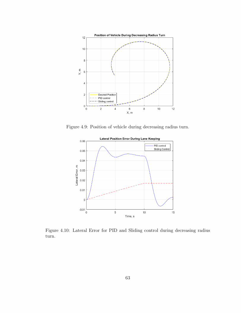
Figure 4.9: Position of vehicle during decreasing radius turn.
Figure 4.10: Lateral Error for PID and Sliding control during decreasing radiusturn.
63
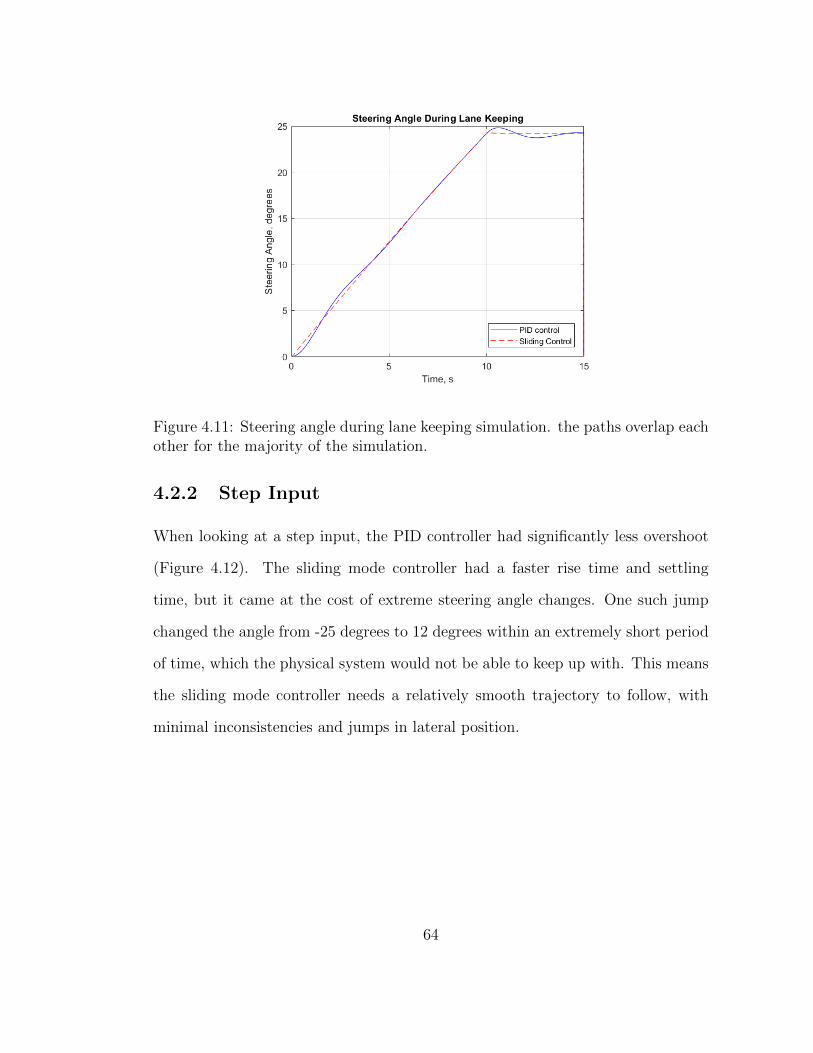
Figure 4.11: Steering angle during lane keeping simulation. the paths overlap eachother for the majority of the simulation.
4.2.2 Step Input
When looking at a step input, the PID controller had significantly less overshoot
(Figure 4.12). The sliding mode controller had a faster rise time and settling
time, but it came at the cost of extreme steering angle changes. One such jump
changed the angle from -25 degrees to 12 degrees within an extremely short period
of time, which the physical system would not be able to keep up with. This means
the sliding mode controller needs a relatively smooth trajectory to follow, with
minimal inconsistencies and jumps in lateral position.
64
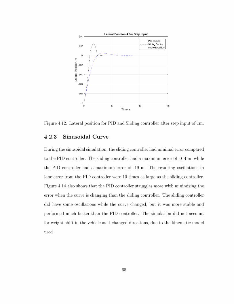
Figure 4.12: Lateral position for PID and Sliding controller after step input of 1m.
4.2.3 Sinusoidal Curve
During the sinusoidal simulation, the sliding controller had minimal error compared
to the PID controller. The sliding controller had a maximum error of .014 m, while
the PID controller had a maximum error of .19 m. The resulting oscillations in
lane error from the PID controller were 10 times as large as the sliding controller.
Figure 4.14 also shows that the PID controller struggles more with minimizing the
error when the curve is changing than the sliding controller. The sliding controller
did have some oscillations while the curve changed, but it was more stable and
performed much better than the PID controller. The simulation did not account
for weight shift in the vehicle as it changed directions, due to the kinematic model
used.
65
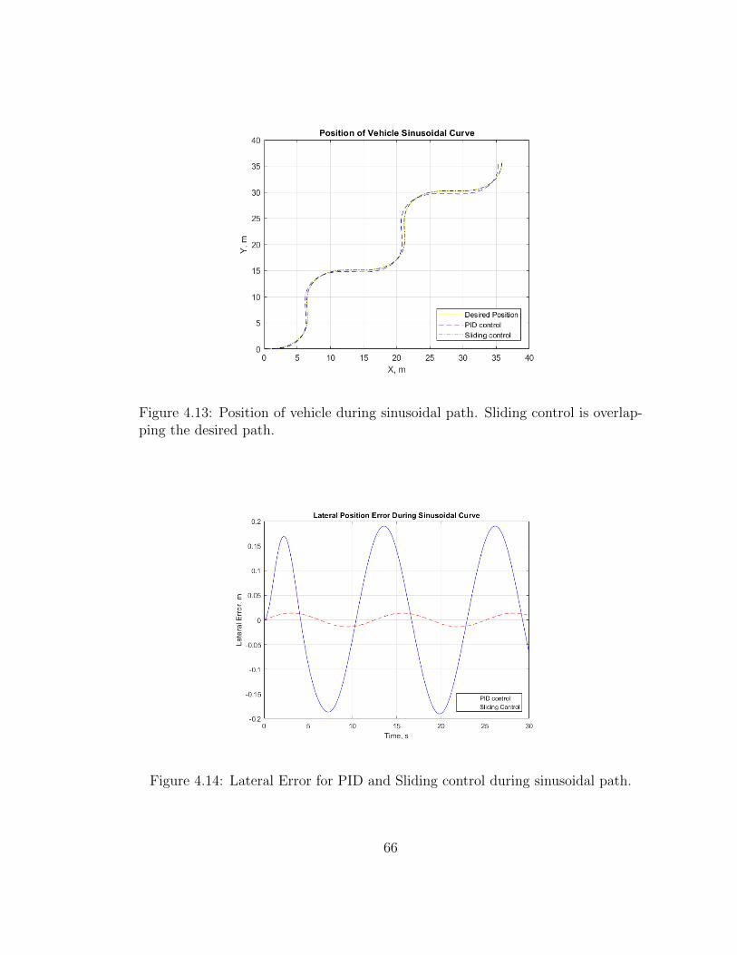
Figure 4.13: Position of vehicle during sinusoidal path. Sliding control is overlap-ping the desired path.
Figure 4.14: Lateral Error for PID and Sliding control during sinusoidal path.
66
Chapter 5
Conclusions and Future Work
5.1 Conclusions
Methods for converting the mechanical systems of a Polaris GEM e2 to drive-
by-wire systems were discussed in this thesis. These changes included replacing
the accelerator pedal with a pair of electronically controlled potentiomenters, in-
stalling a linear actuator onto the master cylinder for the brake, and replacing the
steering wheel and column with a stepper motor and gearbox. The overall control
architecture was also described, including the use of ROS for communications and
hardware integration.
Once the separate systems were explained, a kinematic and dynamic model was
derived to simulate the vehicle. An adaptive trajectory control was proposed for
controlling the vehicles speed. Overall, the adaptive controller outperformed its
PID counterpart by having minimal oscillations and consistently decreasing errors.
When testing acceleration to 2 m/s, the adaptive controller had a maximum error
of -0.0092 m, whereas the PID controller had an error of 0.09 m, which was an
67
order of magnitude larger.
A sliding mode controller was proposed for controlling the steering angle when
path following, and it performed well at keeping the error minimized when com-
pared to a PID controller. The sliding mode controller also performed better on
a sinusoidal curve. However, when faced with a sudden jump in target lateral
position, some of its changes in the steering angle may prove problematic for the
stepper motor to keep up with. This is an issue because the vehicle must be able to
respond well to emergencies, such as people running out in front of the car. Care
must be taken to ensure that the actuator is properly considered, such as including
limits on how fast the sliding mode controller can change the angle.
5.2 Future Work
Autonomous vehicles will continue to be an important research topic in the future.
The proposed methods in this thesis are expected to be used for IGVC. In order to
utilize these features outside the scope of the competition, several improvements
should be considered.
5.2.1 Increasing DOF
Several assumptions were made throughout this thesis, including ignoring the pos-
sibility of longitudinal and lateral tire slip. While these assumptions were accept-
able for the lower speed maneuvers required by IGVC, the use of these models is
more limited in higher speed situations. If these limits, such as minimizing lateral
acceleration, are acknowledged and managed properly, then higher speed travel is
fine, but still not ideal. A higher DOF model would allow for applications such as
68
high lateral acceleration motions and more emergency oriented maneuvers.
5.2.2 System Integration
The proposed controllers (velocity and lane keeping) were only tested in a simulated
environment. Integration onto the vehicle is the next logical step. Lane keeping
using a sliding mode controller would require two pieces of information: the lateral
error from lane center, and the difference in angle between the vehicle and the
direction the road is pointed. This data could be found using lane detection with
a stereoscopic camera. Velocity control would require knowledge of the vehicles
speed. This could be done by either accessing the Polaris GEM e2 speedometer or
by using a 3rd party system to measure velocity. The implementation should be
tested in a limited capacity first to minimize risk.
5.2.3 Revise Sliding Mode Controller
The sliding mode controller should have limits in place on how fast it can change
the steering angle. Doing so will allow the controller to work within the stepper
motors limitations. This may require changing the parameters of the control law
to have re-optimize the system.
5.2.4 Utilize Fuzzy Logic
Fuzzy logic controllers are relatively underused in automotive applications. Most
research on this topic has been focused toward velocity control. One of the benefits
of testing a fuzzy logic control system is that it can be integrated with other control
laws or used on its own. Fuzzy logic could apply well to lane keeping, since it would
69

be able to handle uncertainties such as changing road conditions without having
to use processing power to estimate new parameters.
70
Bibliography
[1] Autonomous vehicles: Coming to a road near you. Government Technology,
31(5):38–41, 2018.
[2] National Highway Traffic Safety Administration. A drive through time.
https://one.nhtsa.gov/nhtsa/timeline/index.html.
[3] National Highway Traffic Safety Administration. Quick facts 2016.
https://crashstats.nhtsa.dot.gov/Api/Public/ViewPublication/812451, 2017.
[4] National Highway Traffic Safety Administration. Automated vehicles
for safety. https://www.nhtsa.gov/technology-innovation/automated-vehicles-
safety, 2018.
[5] National Highway Traffic Safety Administration. Traffic safety facts. United
States Congress, 2018.
[6] Defense Advance Research Projects Agency. The grand challenge.
https://www.darpa.mil/about-us/timeline/-grand-challenge-for-autonomous-
vehicles.
71
[7] S. Anwar. An anti-lock braking control system for a hybrid electromagnetic/-
electrohydraulic brake-by-wire system. Proceedings of the American Control
Conference, 3:2699–2704, 2004.
[8] C. Becker, L. Yount, S. Rosen-Levy, and J. Brewer. Functional safety as-
sessment of an automated lane centering system (report no. dot hs 812 573).
National Highway Traffic Safety Administration, 2018.
[9] T. Becsi and S. Aradi. Design of lane keeping algorithm of autonomous vehicle.
Periodica Polytechnica: Transportation Engineering, 44(1):60–68, 2016.
[10] S. Bennett. A brief history of automatic control. IEEE Control Systems
Magazine, 16(3):17–25, 1996.
[11] H. Cao, X. Song, S. Zhao, S. Bao, and Z. Huang. An optimal model-based
trajectory following architecture synthesising the lateral adaptive preview strat-
egy and longitudinal velocity planning for highly automated vehicle. Vehicle
System Dynamics, 55(8):1143–1188, 2017.
[12] R. Chase. Does everyone in america own a car? United States Congress, 2010.
[13] Jeff Davis. Dreaming of driverless: Whats the difference between level 2
and level 5 autonomy? https://blogs.nvidia.com/blog/2018/01/25/whats-
difference-level-2-level-5-autonomy/, 2018.
[14] R. DeCarlo and S. Zak. A quick introduction to sliding mode control and its
applications. Universita Degli Studi Di Cagliari, 2008.
[15] Dewesoft. Pid control. https://dewesoft.pro/online/course/pid-control.
72
[16] R. Dorf and R. Bishop. Modern Control Systems, 8th edition. Addison-Wesley,
Reading, MA, 1998.
[17] Neural Dump. Stanley the volkswagen wins grand challenge 2005.
https://www.neuraldump.net/2005/10/stanley-the-volkswagen-wins-grand-
challenge-2005, 2005.
[18] T. Gillespie. Fundamentals of vehicle dynamics. SAE International, 1:1–519,
2001.
[19] P. Gora and I. Rub. Traffic models for self-driving connected cars. Trans-
portation Research Procedia, 14:2207–2219, 2016.
[20] B. Guvenc, L. Guvenc, D. Odenthal, and T. Bunte. Robust two degree of
freedom vehicle steering control satisfying mixed sensitivity constraint. IEEE
Transactions on Control Systems Technology, 12:627–636, 2001.
[21] L. Han, H. Yashiro, H. Nejad, Q. Do, and S. Mita. Bezier curve based path
planning for autonomous vehicle in urban environment. IEEE Intelligent Ve-
hicle Symposium, San Diego, CA, pages 1036–1042, 2010.
[22] L. Hoberock. A survey of longitudinal acceleration comfort studies in ground
transportion vehicles. U.S. Department of Transportation, 1976.
[23] IGVC. Igvc 2019 rules. www.igvc.org/2019rules.pdf.
[24] National Instruments. Pid theory explained. http://www.ni.com/en-
us/innovations/white-papers/06/pid-theory-explained.html, 2019.
73
[25] SAE International. Sae international releases updated visual chart
for its levels of driving automation standard for self-driving vehicles.
www.sae.org/news/press-room/2018/12/sae-international-releases-updated-
visual-chart-for-its-levels-of-driving-automation-standard-for-self-driving-
vehicles, 2018.
[26] J. Jaafar and E. McKenzie. Decision making method using fuzzy logic for
autonomous agent navigation. Journal of Computer Science and Information
Technology, 3(1):8–18, 2011.
[27] J. Jang, C. Sun, and E. Mizutani. Neuro-fuzzy and soft computing, a com-
putational approach to learning and machine intelligence. IEEE Transactions
on Automatic Control, 42(10):1482–1485, 1997.
[28] E. Jones and R. Childers. Contemporary College Physics - 2nd Edition. 1993.
[29] N. Leveson. Adaptive cruise control system overview. 5th Meeting of the U.S.
Software System Safety Working Group, Anaheim, CA, 2005.
[30] Y. Li, P. Musilek, and L. Wyard-Scott. Fuzzy logic in agent-based game
design. IEEE Annual Meeting of the Fuzzy Information, Alberta, Canada,
2:734–739, 2004.
[31] S. Mostafa, A. Mustapha, M. Mohammed, M. Ahmad, and M. Mahmoud.
A fuzzy logic control in adjustable autonomy of a multi-agent system for an
automated elderly movement monitoring application. International Journal of
Medical Informatics, 112:173–184, 2018.
[32] Oriental Motors. Ard-kd user manual for ac and dc systems.
www.orientalmotor.com/products/pdfs/opmanuals/HM-60340-2E.pdf.
74
[33] J. Naranjo, C. Gonzalez, J. Reviejo, R. Garcia, and T. Pedro. Adaptive
fuzzy control for inter-vehicle gap keeping. IEEE Transactions On Intelligent
Transportation Systems, 4(3):132–142, 2003.
[34] Society of Automotive Engineers. Vehicle dynamics terminalogy. J670 200801,
2008.
[35] US Department of Transportation. Vehicle nonlinear equations of motion.
https://users.ece.cmu.edu/ koopman/ahs/ahs objectives/AHS8.pdf, January
10, 2019.
[36] H. Pacejka, E. Bakker, and L. Nyborg. Tyre modelling for use in vehicle
dynamics studies. SAE International Congress and Exposition, paper number:
870421, 1987.
[37] R. Pepy, A. Lambert, and H. Mournier. Path planning using a dynamic vehicle
model. IEEE 2nd International Conference on Information and Communica-
tion Technologies, 1:781–786, 2006.
[38] Polaris. Model specifications specs: Gem e2. gem.polaris.com/en-
us/e2/specs/.
[39] M. Quigley, B. Gerkey, and W. Smart. Programming Robots with ROS (1st
ed.). O’Reilly Media, Sebastopol, CA, 2015.
[40] R. Rajamani. Vehicle Dynamics and Control 2nd Edition. Springer, New
York, NY, 2012.
[41] R. Rajamani and C. Zhu. Semi-autonomous adaptive cruise control systems.
IEEE Transactions on Vehicular Technology, 51(5):1186–1192, 2002.
75
[42] P. Ramanata. Optimal vehicle path generator using optimization methods.
Virginia Polytechnic Institute, 1998.
[43] R. Rojas. Spirit of berlin: An autonomous car for the darpa urban challenge
hardware and software architecture. DARPA Grand Challenge, 2007.
[44] ROS. Core components. http://www.ros.org/core-components/.
[45] ROS. History. http://www.ros.org/history/, 2019.
[46] H. Seo, S. Youn, and K. Oh. A fuzzy reinforcement function for the intelligent
agent to process vague goals. IEEE 19th International conference of the North
American, Atlanta, GA, 8:29–33, 2000.
[47] J. Setiawan, M. Safarudin, and A. Singh. Modeling, simulation and validation
of 14 dof full vehicle model. IEEE International Conference on Instrumenta-
tion, Communication, Information Technology, and Biomedical Engineering,
Indonesia, pages 1–6, 2009.
[48] M. Short and M. Pont. Simulation of vehicle longitudinal dynamics. Embedded
Systems Laboratory, 2004.
[49] J. Slotine and W. Li. Applied Nonlinear Control, 2nd Edition. Prentice-Hall,
Englewood Cliffs, NJ, 1991.
[50] M. Tanelli, R. Sartori, and S. Savaresi. Combining slip and deceleration control
for brake-by-wire control systems: A sliding-mode approach. European Journal
of Control, 13(6):593–611, 2007.
[51] Trinamic. Pd86-3-1180. www.trinamic.com/products/drives/stepper-
pandrives-details/pd86-3-1180/.
76
[52] H. Unbehauen. Control Systems, Robotics and Automation- Volume II.
EOLSS Publishers, Oxford, UK, 2009.
[53] A. Vahidi and A. Eskandarian. Research advances in intelligent collision avoid-
ance and adaptive cruise control. IEEE Transactions On Intelligent Transporta-
tion Systems, 4(3):143–153, 2003.
[54] S. Vijayabaskar and T. Manigandan. Performance analysis of permanent
magnet synchronous motor using hybrid optimization algorithm. International
Journal of Advanced Engineering Technology, 7(2):748–753, 2016.
[55] C. Wen. Globally stable single loop and decentralized adaptive systems with
parameter projection. Control and Dynamic Systems, 72:301–345, 1995.
[56] W. Xiang, P. Richardson, C. Zhao, and S. Mohammed. Automobile brake-
by-wire control system design and analysis. IEEE Transactions on Vehicular
Technology, 57(1):138–145, 2008.
[57] Y. Yamaguchi and T. Murakami. Adaptive control for virtual steering char-
acteristics on electric vehicle using steer-by-wire system. IEEE Transactions
on Industrial Electronics, 56(5):1585–1594, 2009.
77


![Technical Bulletin - Polaris - Polaris 9300 Sport & Polaris 9300xi Sport[1]](https://img.pdfslide.us/doc/110x75/553b235d4a7959d8258b463f/technical-bulletin-polaris-polaris-9300-sport-polaris-9300xi-sport1.jpg)