Accelerating SPARQL Queries by Exploiting Hash-basedLocality and Adaptive Partitioning

Razen Harbi · Ibrahim Abdelaziz · Panos Kalnis · Nikos Mamoulis ·

Yasser Ebrahim · Majed Sahli

Abstract State-of-the-art distributed RDF systems par-

tition data across multiple computer nodes (workers).

Some systems perform cheap hash partitioning, whichmay result in expensive query evaluation. Others try to

minimize inter-node communication, which requires an

expensive data pre-processing phase, leading to a highstartup cost. Apriori knowledge of the query workload

has also been used to create partitions, which however

are static and do not adapt to workload changes.

In this paper, we propose AdPart, a distributed

RDF system, which addresses the shortcomings of pre-

vious work. First, AdPart applies lightweight partition-ing on the initial data, that distributes triples by hash-

ing on their subjects; this renders its startup overhead

low. At the same time, the locality-aware query opti-mizer of AdPart takes full advantage of the partition-

ing to (i) support the fully parallel processing of join

patterns on subjects and (ii) minimize data communi-

cation for general queries by applying hash distributionof intermediate results instead of broadcasting, wher-

ever possible. Second, AdPart monitors the data access

patterns and dynamically redistributes and replicatesthe instances of the most frequent ones among workers.

As a result, the communication cost for future queries is

drastically reduced or even eliminated. To control repli-cation, AdPart implements an eviction policy for the

redistributed patterns. Our experiments with synthetic

R. Harbi · I. Abdelaziz · P. Kalnis · M. SahliKing Abdullah University of Science & Technology, Thuwal,Saudi ArabiaE-mail: {first}.{last}@kaust.edu.sa

N. MamoulisUniversity of Ioannina, GreeceE-mail: nikos@cs.uoi.gr

Y. EbrahimMicrosoft Corporation, Redmond, WA 98052, United StatesE-mail: yaelsa@microsoft.com

and real data verify that AdPart: (i) starts faster than

all existing systems; (ii) processes thousands of queries

before other systems become online; and (iii) gracefullyadapts to the query load, being able to evaluate queries

on billion-scale RDF data in sub-seconds.

1 Introduction

The RDF data model does not require a predefinedschema and represents information from diverse sources

in a versatile manner. Therefore, social networks, search

engines, shopping sites and scientific databases are adopt-

ing RDF for publishing web content. Large public knowl-edge bases, such as Bio2RDF1 and YAGO2 have bil-

lions of facts in RDF format. RDF datasets consist of

triples of the form 〈subject, predicate, object〉, wherepredicate represents a relationship between two enti-

ties: a subject and an object. An RDF dataset can be

regarded as a long relational table with three columns.An RDF dataset can also be viewed as a directed la-

beled graph, where vertices and edge labels correspond

to entities and predicates, respectively. Figure 1 shows

an example RDF graph of an academic network.

SPARQL3 is the standard query language for RDF.

Each query is a set of RDF triple patterns; some of

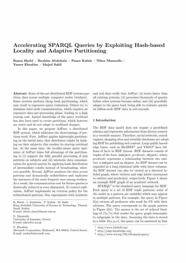
the nodes in a pattern are variables which may appearin multiple patterns. For example, the query in Figure

2(a) returns all professors who work for CS with their

advisees. The query corresponds to the graph patternin Figure 2(b). The answer is the set of ordered bind-

ings of (?p, ?s) that render the query graph isomorphic

to subgraphs in the data. Assuming the data is storedin a table D(s, p, o), the query can be answered by first

1 http://www.bio2rdf.org/2 http://yago-knowledge.org/3 http://www.w3.org/TR/rdf-sparql-query/

2 Razen Harbi et al.

Fig. 1 Example RDF graph. An edge and its associated ver-tices correspond to an RDF triple; e.g., 〈Bill, worksFor, CS〉.

Fig. 2 A query that finds CS professors with their advisees.

decomposing it into two subqueries, each correspond-ing to a triple pattern: q1 ≡ σp=worksFor∧o=CS(D) and

q2 ≡ σp=advisor(D). The subqueries can be answered

independently by scanning table D; then, we can join

their intermediate results on the subject and object at-tribute: q1 ⊲⊳q1.s=q2.o q2. By applying the query on the

data of Figure 1, we get (?prof, ?stud) ∈ {(James,

Lisa),(Bill, John), (Bill, Fred),(Bill, Lisa)}.

Early research efforts on RDF data management re-sulted in efficient centralized RDF systems; like RDF-

3X [25], HexaStore [33], TripleBit [36] and gStore [40].

However, centralized data management does not scale

well for complex queries on web-scale RDF data. As aresult, distributed RDF management systems were in-

troduced to scale-out by partitioning RDF data among

many compute nodes (workers) and evaluating queriesin a distributed fashion. A SPARQL query is decom-

posed into multiple subqueries that are evaluated by

each node independently. Since data is distributed, thenodes may need to exchange intermediate results during

query evaluation. Consequently, queries with large in-

termediate results incur high communication cost, which

is detrimental to the query performance [16,19].

Distributed RDF systems aim at minimizing thenumber of decomposed subqueries by partitioning the

data among workers. The goal is that each node has

all the data it needs to evaluate the entire query andthere is no need for exchanging intermediate results. In

such a parallel query evaluation, each node contributes

a partial result of the query; the final query result is the

union of all partial results. To achieve this, some triplesmay need to be replicated across multiple partitions.

For example, in Figure 1, assume the data graph is di-

vided by the dotted line into two partitions and assume

that triples follow their subject placement. To answer

the query in Figure 2, nodes have to exchange inter-mediate results because triples 〈Lisa, advisor, Bill〉

and 〈Fred, advisor, Bill〉 cross the partition boundary.

Replicating these triples to both partitions allows eachnode to answer the query without communication. Still,

even sophisticated partitioning and replication cannot

guarantee that arbitrarily complex SPARQL queriescan be processed in parallel; thus, expensive distributed

query evaluation, with intermediate results exchanged

between nodes, cannot always be avoided.

Challenges. Existing distributed RDF systems are fac-

ing two limitations. (i) Partitioning cost: balanced graph

partitioning is an NP-complete problem [22]; thus, ex-isting systems perform heuristic partitioning. In sys-

tems that use simple hash partitioning heuristics [17,

26,29,38], queries have low chances to be evaluated in

parallel without communication between nodes. On theother hand, systems that use sophisticated partitioning

heuristics [16,19,23,34] suffer from high preprocessing

cost and sometimes high replication. More importantly,they pay the cost of partitioning the entire data regard-

less of the anticipated workloads. However, as shown in

a recent study [28], only a small fraction of the wholegraph is accessed by typical real query workloads. For

example, a real workload consisting of more than 1,600

queries executed on DBpedia (459M triples) touches

only 0.003% of the whole data. Thus, we argue that dis-tributed RDF systems should leverage query workloads

in data partitioning. (ii) Adaptivity: WARP [18] and

Partout [13] do consider the workload during data par-titioning and achieve significant reduction in the repli-

cation ratio, while showing better query performance

compared to systems that partition the data blindly.Nonetheless, both these systems assume a representa-

tive (i.e., static) query workload and do not adapt to

changes. Aluc et al. [1] showed that systems need to

continuously adapt to workloads in order to consistentlyprovide good performance.

In this paper, we propose AdPart, a distributed in-

memory RDF engine. AdPart alleviates the aforemen-

tioned limitations of existing systems by capitalizing onthe following key principles:

Lightweight Initial Partitioning: AdPart uses an

initial hash partitioning that distributes triples by hash-

ing on their subjects. This partitioning has low cost anddoes not incur any replication. Thus, the preprocessing

time is low, partially addressing the first challenge.

Hash-based Locality Awareness: AdPart exploits

hash-based locality to process in parallel (i.e., with-out data communication) the join patterns on subjects

included in a query. In addition, intermediate results

can potentially be hash-distributed to single workers

Accelerating SPARQL Queries by Exploiting Hash-based Locality and Adaptive Partitioning 3

instead of being broadcasted everywhere. The locality-

aware query optimizer of AdPart considers these prop-erties to generate an evaluation plan that minimizes

intermediate results shipped between workers.

Adapting by Incremental Redistribution: A hi-erarchical heat-map of accessed data patterns is main-

tained by AdPart to monitor the executed workload.

Hot patterns are redistributed and potentially repli-cated in the system in a way that future queries that

include them are executed in parallel by all workers

without data communication. To control replication,

AdPart operates within a budget and employs an evic-tion policy for the redistributed patterns. By adapt-

ing dynamically to the workload, AdPart overcomes the

limitations of static partitioning schemes.

In summary, our contributions are:

– We introduce AdPart, a distributed SPARQL en-

gine that does not require expensive preprocessing.

By using lightweight hash partitioning, avoiding theupfront cost, and adopting a pay-as-you-go approach,

AdPart executes tens of thousands of queries on

large graphs within the time it takes other systemsto conduct their initial partitioning.

– We propose a locality-aware query planner and a

cost-based optimizer for AdPart to efficiently exe-

cute queries that require data communication.– We propose the monitoring and indexing workloads

in the form of hierarchical heat maps. Queries are

transformed and indexed using these maps to facil-itate the adaptivity of AdPart. We introduce an In-

cremental ReDistribution (IRD) technique for data

portions that are accessed by hot patterns, guidedby the workload. IRD helps processing future queries

without data communication.

– We evaluate AdPart using synthetic and real data

and compare with state-of-the-art systems. AdPartpartitions billion-scale RDF data and starts up in

less than 14 minutes, while other systems need hours

or days. On billion-scale RDF data, AdPart executescomplex queries in sub-seconds and processes large

workloads orders of magnitude faster than existing

approaches.

The rest of the paper is organized as follows. Section2 reviews existing distributed RDF systems. Section 3

presents the architecture of AdPart and provides an

overview of the system’s components. Section 4 discuses

our locality-aware query planning and distributed queryevaluation, whereas Section 5 explains the adaptivity

feature of AdPart. Section 6 contains the experimental

results and Section 7 concludes the paper.

2 Related Work

In this section, we review recent distributed RDF sys-tems related to AdPart. Table 1, summarizes the main

characteristics of these systems.

Lightweight Data Partitioning: Several systemsare based on the MapReduce framework [8] and use

the Hadoop Distributed File System (HDFS), which ap-

plies horizontal random data partitioning. SHARD [29]

stores the whole RDF data in one HDFS file. Similarly,HadoopRDF [20] uses HDFS but splits the data into

multiple smaller files. SHARD and HadoopRDF solve

SPARQL queries using a set of MapReduce iterations.

Trinity.RDF [38] is a distributed in-memory RDF

engine that can handle web scale RDF data. It rep-resents RDF data in its native graph form (i.e., using

adjacency lists) and uses a key-value store as the back-

end store. The RDF graph is partitioned using vertexid as hash key. This is equivalent to partitioning the

data twice; first using subjects as hash keys and sec-

ond using objects. Trinity.RDF uses graph explorationfor SPARQL query evaluation and relies heavily on its

underlying high-end InfiniBand interconnect. In every

iteration, a single subquery is explored starting from

valid bindings by all workers. This way, generation ofredundant intermediate results is avoided. However, be-

cause exploration only involves two vertices (source and

target), Trinity.RDF cannot prune invalid intermediateresults without carrying all their historical bindings.

Hence, workers need to ship candidate results to the

master to finalize the results, which is a potential bot-tleneck of the system.

Rya [27] and H2RDF+ [26] use key-value stores forRDF data storage which range-partition the data based

on keys such that the keys in each partition are sorted.

When solving a SPARQL query, Rya executes the firstsubquery using range scan on the appropriate index;

it then utilizes index lookups for the next subqueries.

H2RDF+ executes simple queries in a centralized fash-ion, whereas complex queries are solved using a set of

MapReduce iterations.

All the above systems use lightweight partitioning

schemes, which are computationally inexpensive; how-

ever, queries with long paths and complex structures in-cur high communication costs. In addition, systems that

evaluate joins using MapReduce suffer from its high

overhead [16,34]. Although our AdPart system also uses

lightweight hash partitioning, it avoids excessive datashuffling by exploiting hash-based data locality. Fur-

thermore, it adapts incrementally to the workload to

further minimize communication.

4 Razen Harbi et al.

Table 1 Summary of state-of-the-art distributed RDF systems

SystemPartitioning

Strategy

Partitioning

CostReplication

Workload

AwarenessAdaptive

TriAD-SG [16] Graph-based (METIS) & Horizontal triple Sharding High Yes No No

H-RDF-3X [19] Graph-based (METIS) High Yes No No

Partout [13] Workload-based horizontal fragmentation High No Yes No

SHAPE [23] Semantic Hash High Yes No No

Wu et al. [34] End-to-end path partitioning Moderate Yes No No

TriAD [16] Hash-based triple Sharding Low Yes No No

Trinity.RDF [38] Hash Low Yes No No

H2RDF+ [26] H-Base partitioner (range) Low No No No

SHARD [29] Hash Low No No No

AdPart Hash Low Yes Yes Yes

Sophisticated Partitioning Schemes and Repli-

cation: Several systems employ general graph parti-

tioning techniques for RDF data, in order to improvedata locality. EAGRE [39] transforms the RDF graph

into a compressed entity graph that is partitioned using

a MinCut algorithm, such as METIS [22]. H-RDF-3X[19] uses METIS to partition the RDF graph among

workers. It also enforces the so-called k-hop guaran-

tee so any query with radius k or less can be exe-cuted without communication. Other queries are ex-

ecuted using expensive MapReduce joins. Replication

increases exponentially with k; thus, k must be small

(e.g., k ≤ 2 in [19]). Both EAGRE and H-RDF-3X suf-fer from the significant overhead of MapReduce-based

joins for queries that cannot be evaluated locally. For

such queries, sub-second query evaluation is not possi-ble [16], even with state-of-the-art MapReduce imple-

mentations, like Hadoop++ [9] and Spark [37].

TriAD [16] employs lightweight hash partitioning

based on both subjects and objects. Since partitioning

information is encoded into the triples, TriAD has fulllocality awareness of the data and processes large num-

ber of concurrent joins without communication. How-

ever, because TriAD shards one (both) relations whenevaluating distributed merge (hash) joins, the locality

of its intermediate results is not preserved. Thus, if the

sharding column of the previous join is not the cur-

rent join column, intermediate results need to be re-sharded. The cost becomes significant for large inter-

mediate results with multiple attributes. TriAD-SG [16]

uses METIS for data partitioning. Edges that cross par-titions are replicated, resulting in 1−hop guarantee. A

summary graph is defined, which includes a vertex for

each partition. Vertices in this graph are connected bythe cross-partition edges. A query in TriAD-SG is evalu-

ated against the summary graph first, in order to prune

partitions that do not contribute to query results. Then,

the query is evaluated on the RDF data residing in thepartitions retrieved from the summary graph. Multiple

join operators are executed concurrently by all workers,

which communicate via an asynchronous message pass-

ing protocol. Sophisticated partitioning techniques, like

MinCut, reduce the communication cost significantly.

However, such techniques are prohibitively expensiveand do not scale for large graphs, as shown in [23].

Furthermore, MinCut does not yield good partition-

ing for dense graphs. Thus, TriAD-SG does not benefitfrom the summary graph pruning technique in dense

RDF graphs because of the high edge-cut. To alleviate

METIS overhead, an efficient approach for partitioninglarge graphs was introduced [32]. However, queries that

cross partition boundaries result in poor performance.

SHAPE [23] is based on a semantic hash portion-ing approach for RDF data. It starts by simple hash

partitioning and employs the same k-hop strategy as

H-RDF-3X [19]. It also relies on URI hierarchy, forgrouping vertices to increase data locality. Similar to

H-RDF-3X, SHAPE suffers from the high overhead of

MapReduce-based joins. Furthermore, URI-based group-

ing results in skewed partitioning if a large percentageof vertices share prefixes. This behavior is noticed in

both real as well as synthetic datasets (See Section 6).

Recently, Wu et al. [34] proposed an end-to-end pathpartitioning scheme, which considers all possible di-

rected paths in the RDF graph. These paths are merged

in a bottom-up fashion. While this approach works wellfor star, chain and directed cyclic queries, other types

of queries result in significant communication. For ex-

ample, queries with object-object joins or queries thatdo not associate each query vertex with the type predi-

cate require inter-worker communication. Note that our

adaptivity technique (Section 5) is orthogonal to and

can be combined with end-to-end path partitioning aswell as other partitioning heuristics to efficiently eval-

uate queries that are not favored by the partitioning.

Workload-Aware Data Partitioning: Most of the

aforementioned partitioning techniques focus on min-

imizing communication without considering the work-

load. Partout [13] is a workload-aware distributed RDFengine. First, it extracts representative triple patterns

from the query load. Then, it uses these patterns to

partition the data into fragments and collocates data

Accelerating SPARQL Queries by Exploiting Hash-based Locality and Adaptive Partitioning 5

fragments that are accessed together by queries in the

same worker. Similarly, WARP [18] uses a represen-tative query workload to replicate frequently accessed

data. Partout and WARP adapt only by applying ex-

pensive re-partitioning of the entire data; otherwise,they incur high communication costs for dynamic work-

loads. On the contrary, our system adapts incrementally

by replicating only the data accessed by the workloadwhich is expected to be small [28].

SPARQL on Vertex-centric: Sedge [35] solves the

problem of dynamic graph partitioning and demonstrates

its partitioning effectiveness using SPARQL queries overRDF. The entire graph is replicated several times and

each replica is partitioned differently. Every SPARQL

query is translated manually into a Pregel [24] program

and is executed against the replica that minimizes com-munication. Still, this approach incurs excessive repli-

cation, as it duplicates the entire data several times.

Moreover, its lack of support for ad-hoc queries makesit counter-productive; a user needs to manually write

an optimized query evaluation program in Pregel.

Materialized views: Several works attempt to speed

up the execution of SPARQL queries by materializinga set of views [6,15] or a set of path expressions [10].

The selection of views is based on a representative work-

load. Our approach does not generate local materialized

views. Instead, we redistribute the data accessed by hotpatterns in a way that preserves data locality and allows

queries to be executed with minimal communication.

Relational Model: Relevant systems exist that focus

on data models other than RDF. Schism [7] deals withdata placement for distributed OLTP RDBMS. Using

a sample workload, Schism minimizes the number of

distributed transactions by populating a graph of co-accessed tuples. Tuples accessed in the same transac-

tion are put in the same server. This is not appropriate

for SPARQL because some queries access large parts of

the data that would overload a single machine. Instead,AdPart exploits parallelism by executing such a query

across all machines in parallel without communication.

H-Store [31] is an in-memory distributed RDBMS thatuses a data partitioning technique similar to ours. Nev-

ertheless, H-Store assumes that the schema and the

query workload are given in advance and assumes noad-hoc queries.

Eventual indexing: Idreos et al. [21] introduced the

concept of reducing the data-to-query time for rela-

tional data. They avoid building indices during data

loading; instead, they reorder tuples incrementally dur-ing query processing. In AdPart, we extend eventual

indexing to dynamic and adaptive graph partitioning.

In our problem, graph partitioning is very expensive;

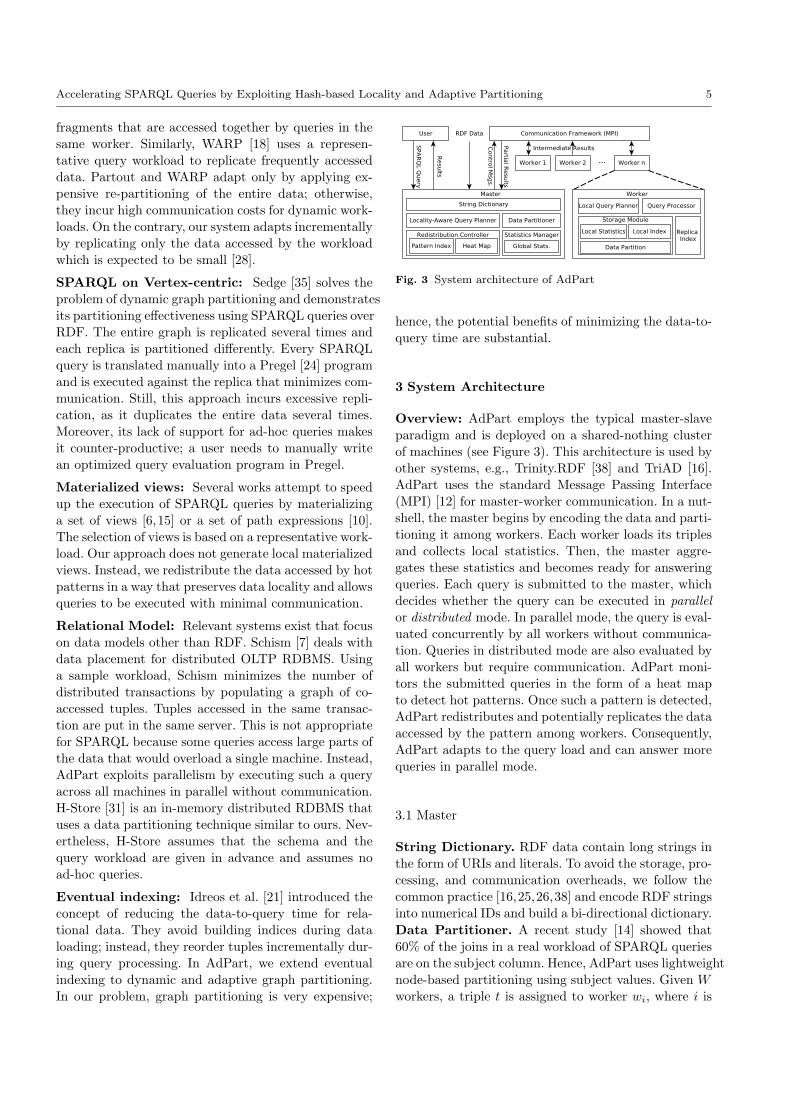
Fig. 3 System architecture of AdPart

hence, the potential benefits of minimizing the data-to-

query time are substantial.

3 System Architecture

Overview: AdPart employs the typical master-slaveparadigm and is deployed on a shared-nothing cluster

of machines (see Figure 3). This architecture is used by

other systems, e.g., Trinity.RDF [38] and TriAD [16].AdPart uses the standard Message Passing Interface

(MPI) [12] for master-worker communication. In a nut-

shell, the master begins by encoding the data and parti-

tioning it among workers. Each worker loads its triplesand collects local statistics. Then, the master aggre-

gates these statistics and becomes ready for answering

queries. Each query is submitted to the master, whichdecides whether the query can be executed in parallel

or distributed mode. In parallel mode, the query is eval-

uated concurrently by all workers without communica-tion. Queries in distributed mode are also evaluated by

all workers but require communication. AdPart moni-

tors the submitted queries in the form of a heat map

to detect hot patterns. Once such a pattern is detected,AdPart redistributes and potentially replicates the data

accessed by the pattern among workers. Consequently,

AdPart adapts to the query load and can answer morequeries in parallel mode.

3.1 Master

String Dictionary. RDF data contain long strings in

the form of URIs and literals. To avoid the storage, pro-cessing, and communication overheads, we follow the

common practice [16,25,26,38] and encode RDF strings

into numerical IDs and build a bi-directional dictionary.

Data Partitioner. A recent study [14] showed that

60% of the joins in a real workload of SPARQL queriesare on the subject column. Hence, AdPart uses lightweight

node-based partitioning using subject values. Given W

workers, a triple t is assigned to worker wi, where i is

6 Razen Harbi et al.

the result of a hash function applied on t.subject.4 This

way all triples that share the same subject go to thesame worker. Consequently, any star query joining on

subjects can be evaluated without communication cost.

We do not hash on objects because they can be literalsand common types; this would assign all triples of the

same type to one worker, resulting in load imbalance

and limited parallelism [19].

Statistics Manager. It maintains statistics about the

RDF graph, which are used for global query planning

and during adaptivity. Statistics are collected in a dis-tributed manner during bootstrapping.

Redistribution Controller. It monitors the workload

in the form of heat maps and triggers the adaptive In-

cremental ReDistribution (IRD) process for hot pat-terns. Data accessed by hot patterns are redistributed

and potentially replicated among workers. A redistributed

hot pattern can be answered by all workers in paral-lel without communication. Replicated hot patterns are

indexed in a structure called Pattern Index (PI). Pat-

terns in the PI can be combined for evaluating futurequeries without communication. Further, the controller

implements replica replacement policy to keep replica-

tion within a threshold (Section 5).

Locality-Aware Query Planner. Our planner usesthe global statistics from the statistics manager and the

pattern index from the redistribution controller to de-

cide if a query, in whole or partially, can be processedwithout communication. Queries that can be fully an-

swered without communication are planned and exe-

cuted by each worker independently. On the other hand,for queries that require communication, the planner ex-

ploits the hash-based data locality and the query struc-

ture to find a plan that minimizes communication and

the number of distributed joins (Section 4).

Failure Recovery. The master does not store any data

but can be considered as a single-point of failure be-

cause it maintains the dictionaries, global statistics, andPI. A standard failure recovery mechanism (log-based

recovery [11]) can be employed by AdPart. Assuming

stable storage, the master can recover by loading thedictionaries and global statistics because they are read-

only and do not change in the system. The PI can be

recovered by reading the query log and reconstructingthe heat map. Workers on the other hand store data;

hence, in case of a failure, data partitions need to be re-

covered. Shen et al. [30] proposes a fast failure recovery

solution for distributed graph processing systems. Thesolution is a hybrid of checkpoint-based and log-based

recovery schemes. This approach can be used by AdPart

to recover worker partitions and reconstruct the replica

4 For simplicity, we use: i = t.subject mod W .

index. Reliability is outside the scope of this paper and

we leave it for future work.

3.2 Worker

Storage Module. Each worker wi stores its local set

of triples Di in an in-memory data structure, which

supports the following search operations, where s, p,

and o are subject, predicate, and object:

1. given p, return set {(s, o) | 〈s, p, o〉 ∈ Di}.2. given s and p, return set {o | 〈s, p, o〉 ∈ Di}.

3. given o and p, return set {s | 〈s, p, o〉 ∈ Di}.

Since all the above searches require a known predicate,

we primarily hash triples in each worker by predicate.The resulting predicate index (simply P-index) imme-

diately supports search by predicate (i.e., the first op-

eration). Furthermore, we use two hash maps to re-partition each bucket of triples having the same predi-

cate, based on their subjects and objects, respectively.

These two hash maps support the second and third

search operation and they are called predicate-subjectindex (PS-index) and predicate-object index (PO-index),

respectively. Given the number of unique predicates is

typically small, our storage scheme avoids unnecessaryrepetitions of predicate values. Note that when answer-

ing a query, if the predicate itself is a variable, then we

simply iterate over all predicates. Our indexing schemeis tailored for typical RDF knowledge bases and their

workloads, being orthogonal to the rest of the system

(i.e., alternative schemes, like indexing all SPO combi-

nations [25] could be used at each worker). Finally, thestorage module computes statistics about its local data

and shares them with the master after data loading.

Replica Index. Each worker has an in-memory replicaindex that stores and indexes replicated data as a re-

sult of the adaptivity. This index initially contains no

data and is updated dynamically by the incrementalredistribution (IRD) process (Section 5).

Query Processor. Each worker has a query processor

that operates in two modes: (i) Distributed Mode for

queries that require communication. In this case, thelocality-aware planner of the master devises a global

query plan. Each worker gets a copy of this plan and

evaluates the query accordingly. Workers solve the queryconcurrently and exchange intermediate results (Sec-

tion 4.1). (ii) Parallel Mode for queries that can be an-

swered without communication. In this case, the master

broadcasts the query to all workers. Each worker has allthe data needed for query evaluation; therefore it gen-

erates a local query plan using its local statistics and

executes the query without communication.

Accelerating SPARQL Queries by Exploiting Hash-based Locality and Adaptive Partitioning 7

Table 2 Matching result of q1 on workers w1 and w2.

w1 w2

?prof ?prof

James Bill

Table 3 The final query results q1 ⊲⊳ q2 on both workers.

w1 w2

?prof ?stud ?prof ?stud

James Lisa Bill Lisa

Bill John

Bill Fred

Local Query Planner. Queries executed in parallel

mode are planned by workers autonomously. For exam-ple, star queries joining on the subject are processed

in parallel due to the initial partitioning. Moreover,

queries answered in parallel after the adaptivity pro-

cess are also planned by local query planners.

4 Query Evaluation

A basic SPARQL query consists of multiple subquery

triple patterns: q1, q2, . . . , qn. Each subquery includes

variables or constants, some of which are used to bind

the patterns together, forming the entire query graph(e.g., see Figure 2(b)). A query with n subqueries re-

quires the evaluation of n − 1 joins. Since data are

memory resident and hash-indexed, we favor hash joinsas they prove to be competitive to more sophisticated

join methods [3]. Our query planner devises an ordering

of these subqueries and generates a left-deep join tree,where the right operand of each join is a base subquery

(not an intermediate result). We do not use bushy tree

plans to avoid building indices for intermediate results.

4.1 Distributed Query Evaluation

In AdPart, triples are hash partitioned among many

workers based on subject values. Consequently, subjectstar queries (i.e., all subqueries join on the subject col-

umn) can be evaluated locally in parallel without com-

munication. However, for other types of queries, workersmay have to communicate intermediate results during

join evaluation. For example, consider the query in Fig-

ure 2 and the partitioned data graph in Figure 1. Thequery consists of two subqueries q1 and q2, where:

– q1: 〈?prof, worksFor, CS〉

– q2: 〈?stud, advisor, ?prof〉

The query is evaluated by a single subject-object

join. However, neither of the workers has all the data

Table 4 The final query results q2 ⊲⊳ q1 on both workers.

w1 w2

?prof ?stud ?prof ?stud

James Lisa Bill John

Bill Lisa

Bill Fred

needed for evaluating the entire query; thus, workers

need to communicate. For such queries, AdPart em-ploys the Distributed Semi-Join (DSJ) algorithm. Each

worker scans the PO-index to find all triples matching

q1. The results on workers w1 and w2 are shown in Ta-ble 2. Then, each worker creates a projection on the join

column ?prof and exchanges it with the other worker.

Once the projected column is received, each workercomputes the semi-join q1⋊?prof q2 using its PO-index.

Specifically, w1 probes p = advisor, o = Bill while

w2 probes p = advisor, o = James to their PO-index.

Note that workers also need to evaluate semi-joins us-ing their local projected column. Then, the semi-join

results are shipped to the sender. In this case, w1 sends

〈Lisa, advisor, Bill〉 and 〈Fred, advisor, Bill〉 to w2;no candidate triples are sent from w2 because James

has no advisees on w2. Finally, each worker computes

the final join q1 ⊲⊳?prof q2. The final query results atboth workers are shown in Table 3.

4.1.1 Hash-based data locality

Observation 1 DSJ can benefit from subject hash lo-

cality to minimize communication. If the join column of

the right operand is subject, the projected column of theleft operand is hash distributed by all workers, instead

of being broadcast to every worker.

In our example, since the join column of q2 is the ob-

ject column (?prof), each worker sends the entire join

column to the other worker. However, based on Obser-vation 1, communication can be minimized if the join

order is reversed (i.e., q2 ⊲⊳ q1). In this case, each worker

scans the P-index to find triples matching q2 and createsa projection on ?prof . Then, because ?prof is the sub-

ject of q1, both workers exploit the subject hash-based

locality by partitioning the projection column and com-municating each partition to the respective worker, as

opposed to broadcasting the entire projection column

to all workers. Consequently, w1 sends Bill to only

w2 because of Bill’s hash value. The final query resultsare shown in Table 4. Notice that the final results are

the same for both query plans; however, the results re-

ported by each worker are different.

8 Razen Harbi et al.

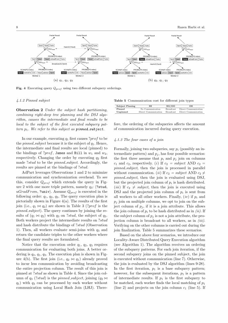
(a) q1, q2, q3 (b) q2, q1, q3

Fig. 4 Executing query Qprof using two different subquery orderings.

4.1.2 Pinned subject

Observation 2 Under the subject hash partitioning,

combining right-deep tree planning and the DSJ algo-rithm, causes the intermediate and final results to be

local to the subject of the first executed subquery pat-

tern p1. We refer to this subject as pinned subject.

In our example, executing q1 first causes ?prof to be

the pinned subject because it is the subject of q1. Hence,

the intermediate and final results are local (pinned) tothe bindings of ?prof , James and Bill in w1 and w2,

respectively. Changing the order by executing q2 first

made ?stud to be the pinned subject. Accordingly, theresults are pinned at the bindings of ?stud.

AdPart leverages Observations 1 and 2 to minimize

communication and synchronization overhead. To seethis, consider Qprof which extends the query in Fig-

ure 2 with one more triple pattern, namely q3: 〈?stud,

uGradFrom, ?univ〉. Assume Qprof is executed in thefollowing order: q1, q2, q3. The query execution plan is

pictorially shown in Figure 4(a). The results of the first

join (i.e., q1 ⊲⊳ q2) are shown in Table 3 (?prof is the

pinned subject). The query continues by joining the re-sults of (q1 ⊲⊳ q2) with q3 on ?stud, the subject of q3.

Both workers project the intermediate results on ?stud

and hash distribute the bindings of ?stud (Observation1). Then, all workers evaluate semi-joins with q3 and

return the candidate triples to the other workers where

the final query results are formulated.

Notice that the execution order q1, q2, q3 requires

communication for evaluating both joins. A better or-

dering is q2, q1, q3. The execution plan is shown in Fig-ure 4(b). The first join (i.e., q2 ⊲⊳ q1) already proved

to incur less communication by avoiding broadcasting

the entire projection column. The result of this join is

pinned at ?stud as shown in Table 4. Since the join col-umn of q3 (?stud) is the pinned subject, joining (q2 ⊲⊳

q1) with q3 can be processed by each worker without

communication using Local Hash Join (LHJ). There-

Table 5 Communication cost for different join types

Subject Pinning SS SO/OO OS

Pinned No Communication Broadcast Direct Communication

Unpinned Direct Communication Broadcast Direct Communication

fore, the ordering of the subqueries affects the amountof communication incurred during query execution.

4.1.3 The four cases of a join

Formally, joining two subqueries, say pi (possibly an in-

termediate pattern) and pj , has four possible scenarios:

the first three assume that pi and pj join on columns

c1 and c2, respectively. (i) If c2 = subject AND c2 =pinned subject, then the join is processed in parallel

without communication. (ii) If c2 = subject AND c2 6=

pinned subject, then the join is evaluated using DSJ,but the projected join column of pi is hash distributed.

(iii) If c2 6= subject, then the join is executed using

DSJ and the projected join column of pi is sent fromall workers to all other workers. Finally, (iv) if pi and

pj join on multiple columns, we opt to join on the sub-

ject column of pj , if it is a join attribute. This allows

the join column of pi to be hash distributed as in (ii). Ifthe subject column of pj is not a join attribute, the pro-

jection column is broadcast to all workers, as in (iii).

Verifying on the other columns is carried out during thejoin finalization. Table 5 summarizes these scenarios.

Based on the above four scenarios, we introduce our

Locality-Aware Distributed Query Execution algorithm(see Algorithm 1). The algorithm receives an ordering

of the subquery patterns. For each join iteration, if the

second subquery joins on the pinned subject, the joinis executed without communication (line 7). Otherwise,

the join is evaluated by the DSJ algorithm (lines 9-28).

In the first iteration, p1 is a base subquery pattern;

however, for the subsequent iterations, p1 is a patternof intermediate results. If p1 is the first subquery to

be matched, each worker finds the local matching of p1(line 2) and projects on the join column c1 (line 5). If

Accelerating SPARQL Queries by Exploiting Hash-based Locality and Adaptive Partitioning 9

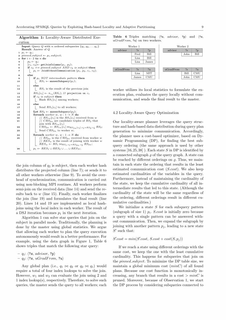
Algorithm 1: Locality-Aware Distributed Exe-cution

Input: Query Q with n ordered subqueries {q1, q2, . . . qn}Result: Answer of Q

1 p1 ← q1;2 pinned subject← p1.subject;3 for i← 2 to n do4 p2 ← qi;5 [c1, c2]← getJoinColumns(p1, p2);6 if c2 == pinned subject AND c2 is subject then7 p1 ← JoinWithoutCommunication (p1, p2, c1, c2);

8 else9 if p1 NOT intermediate pattern then

10 RS1 ← answerSubquery(p1);

11 else12 RS1 is the result of the previous join

13 RS1[c1]← πc1(RS1); // projection on c1

14 if c2 is subject then15 Hash RS1[c1] among workers;

16 else17 Send RS1[c1] to all workers;

18 Let RS2 ← answerSubquery(p2);19 foreach worker w, w : 1→ N do20 // RS1w[c1] is the RS1[c1] received from w21 // CRS2w are candidate triples of RS2 that

join with RS1w[c1]22 CRS2w ← RS1w[c1] ⊲⊳RS1w [c1].c1=RS2.c2

RS2;

23 Send CRS2w to worker w;

24 foreach worker w, w : 1→ N do25 // RS2w is the CRS2w received from worker w

// RESw is the result of joining with worker wRESw ← RS1 ⊲⊳RS1.c1=RS2w.c2

RS2w;

26 p1 ← RES1 ∪ RES2 ∪ .... ∪ RESN ;

the join column of q2 is subject, then each worker hash

distributes the projected column (line 7); or sends it to

all other workers otherwise (line 9). To avoid the over-head of synchronization, communication is carried out

using non-blocking MPI routines. All workers perform

semi-join on the received data (line 14) and send the re-

sults back to w (line 15). Finally, each worker finalizesthe join (line 19) and formulates the final result (line

20). Lines 14 and 19 are implemented as local hash-

joins using the local index in each worker. The result ofa DSJ iteration becomes p1 in the next iteration.

Algorithm 1 can solve star queries that join on the

subject in parallel mode. Traditionally, the planning isdone by the master using global statistics. We argue

that allowing each worker to plan the query execution

autonomously would result in a better performance. For

example, using the data graph in Figure 1, Table 6shows triples that match the following star query:

– q1: 〈?s, advisor, ?p〉

– q2: 〈?s, uGradFrom, ?u〉

Any global plan (i.e., q1 ⊲⊳ q2 or q2 ⊲⊳ q1) would

require a total of four index lookups to solve the join.However, w1 and w2 can evaluate the join using 2 and

1 index lookup(s), respectively. Therefore, to solve such

queries, the master sends the query to all workers; each

Table 6 Triples matching 〈?s, advisor, ?p〉 and 〈?s,uGradFrom, ?u〉 on two workers.

Worker 1 Worker 2

advisor ?s ?p advisor ?s ?p

Fred Bill John Bill

Lisa Bill

Lisa James

uGradFrom ?s ?u uGradFrom ?s ?u

Lisa MIT Bill CMU

James CMU John CMU

worker utilizes its local statistics to formulate the ex-

ecution plan, evaluates the query locally without com-munication, and sends the final result to the master.

4.2 Locality-Aware Query Optimization

Our locality-aware planner leverages the query struc-

ture and hash-based data distribution during query plan

generation to minimize communication. Accordingly,the planner uses a cost-based optimizer, based on Dy-

namic Programming (DP), for finding the best sub-

query ordering (the same approach is used by othersystems [16,25,38] ). Each state S in DP is identified by

a connected subgraph of the query graph. A state can

be reached by different orderings on . Thus, we main-

tain in each state the ordering that results in the leastestimated communication cost (S.cost). We also keep

estimated cardinalities of the variables in the query.

Furthermore, instead of maintaining the cardinality ofthe state, we keep the cumulative cardinality of all in-

termediate results that led to this state. (Although the

cardinality of the state will be the same regardless ofthe ordering, different orderings result in different cu-

mulative cardinalities.)

We initialize a state S for each subquery pattern

(subgraph of size 1) pi. S.cost is initially zero because

a query with a single pattern can be answered with-

out communication. Then, we expand the subgraph byjoining with another pattern pj , leading to a new state

S′ such that:

S′.cost = min(S′.cost, S.cost+ cost(S, pj))

If we reach a state using different orderings with the

same cost, we keep the one with the least cumulativecardinality. This happens for subqueries that join on

the pinned subject. To minimize the DP table size, we

maintain a global minimum cost (minC) of all found

plans. Because our cost function is monotonically in-creasing, any branch that results in a cost > minC is

pruned. Moreover, because of Observation 1, we start

the DP process by considering subqueries connected to

10 Razen Harbi et al.

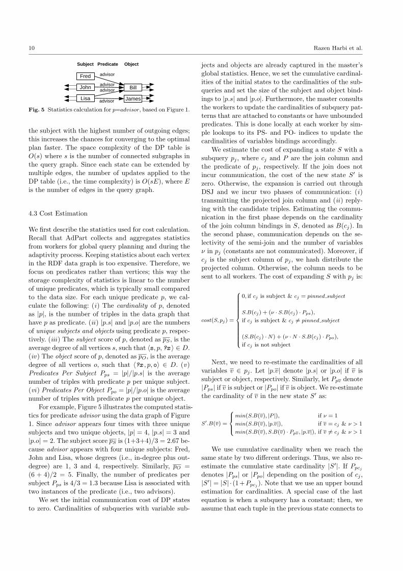
Fig. 5 Statistics calculation for p=advisor, based on Figure 1.

the subject with the highest number of outgoing edges;

this increases the chances for converging to the optimal

plan faster. The space complexity of the DP table isO(s) where s is the number of connected subgraphs in

the query graph. Since each state can be extended by

multiple edges, the number of updates applied to the

DP table (i.e., the time complexity) is O(sE), where Eis the number of edges in the query graph.

4.3 Cost Estimation

We first describe the statistics used for cost calculation.Recall that AdPart collects and aggregates statistics

from workers for global query planning and during the

adaptivity process. Keeping statistics about each vertexin the RDF data graph is too expensive. Therefore, we

focus on predicates rather than vertices; this way the

storage complexity of statistics is linear to the numberof unique predicates, which is typically small compared

to the data size. For each unique predicate p, we cal-

culate the following: (i) The cardinality of p, denoted

as |p|, is the number of triples in the data graph thathave p as predicate. (ii) |p.s| and |p.o| are the numbers

of unique subjects and objects using predicate p, respec-

tively. (iii) The subject score of p, denoted as pS , is theaverage degree of all vertices s, such that 〈s, p, ?x 〉 ∈ D.

(iv) The object score of p, denoted as pO, is the average

degree of all vertices o, such that 〈?x , p, o〉 ∈ D. (v)Predicates Per Subject Pps = |p|/|p.s| is the average

number of triples with predicate p per unique subject.

(vi) Predicates Per Object Ppo = |p|/|p.o| is the average

number of triples with predicate p per unique object.For example, Figure 5 illustrates the computed statis-

tics for predicate advisor using the data graph of Figure

1. Since advisor appears four times with three uniquesubjects and two unique objects, |p| = 4, |p.s| = 3 and

|p.o| = 2. The subject score pS is (1+3+4)/3 = 2.67 be-

cause advisor appears with four unique subjects: Fred,John and Lisa, whose degrees (i.e., in-degree plus out-

degree) are 1, 3 and 4, respectively. Similarly, pO =

(6 + 4)/2 = 5. Finally, the number of predicates per

subject Pps is 4/3 = 1.3 because Lisa is associated withtwo instances of the predicate (i.e., two advisors).

We set the initial communication cost of DP states

to zero. Cardinalities of subqueries with variable sub-

jects and objects are already captured in the master’s

global statistics. Hence, we set the cumulative cardinal-ities of the initial states to the cardinalities of the sub-

queries and set the size of the subject and object bind-

ings to |p.s| and |p.o|. Furthermore, the master consultsthe workers to update the cardinalities of subquery pat-

terns that are attached to constants or have unbounded

predicates. This is done locally at each worker by sim-ple lookups to its PS- and PO- indices to update the

cardinalities of variables bindings accordingly.

We estimate the cost of expanding a state S with a

subquery pj , where cj and P are the join column andthe predicate of pj , respectively. If the join does not

incur communication, the cost of the new state S′ is

zero. Otherwise, the expansion is carried out through

DSJ and we incur two phases of communication: (i)transmitting the projected join column and (ii) reply-

ing with the candidate triples. Estimating the commu-

nication in the first phase depends on the cardinalityof the join column bindings in S, denoted as B(cj). In

the second phase, communication depends on the se-

lectivity of the semi-join and the number of variablesν in pj (constants are not communicated). Moreover, if

cj is the subject column of pj , we hash distribute the

projected column. Otherwise, the column needs to be

sent to all workers. The cost of expanding S with pj is:

cost(S, pj) =

0, if cj is subject & cj = pinned subject

S.B(cj) + (ν · S.B(cj) · Pps),

if cj is subject & cj 6= pinned subject

(S.B(cj) ·N) + (ν ·N · S.B(cj) · Ppo),

if cj is not subject

Next, we need to re-estimate the cardinalities of all

variables v ∈ pj . Let |p.v| denote |p.s| or |p.o| if v is

subject or object, respectively. Similarly, let Ppv denote

|Pps| if v is subject or |Ppo| if v is object. We re-estimatethe cardinality of v in the new state S′ as:

S′.B(v) =

min(S.B(v), |P |), if ν = 1

min(S.B(v), |p.v|), if v = cj & ν > 1

min(S.B(v), S.B(v) · Ppv, |p.v|), if v 6= cj & ν > 1

We use cumulative cardinality when we reach thesame state by two different orderings. Thus, we also re-

estimate the cumulative state cardinality |S′|. If Ppcj

denotes |Pps| or |Ppo| depending on the position of cj ,

|S′| = |S| · (1+Ppcj ). Note that we use an upper boundestimation for cardinalities. A special case of the last

equation is when a subquery has a constant; then, we

assume that each tuple in the previous state connects to

Accelerating SPARQL Queries by Exploiting Hash-based Locality and Adaptive Partitioning 11

this constant by setting Ppcj=1. Note that a more ac-

curate cardinality estimation like the one used in Trin-ity.RDF [38] is orthogonal to our optimizer.

5 AdPart Adaptivity

Studies show that even minimal communication results

in significant performance degradation [19,23]. Thus,

data should be redistributed to minimize, if not elim-

inate, communication and synchronization overheads.AdPart redistributes only the parts of data needed for

the current workload and adapts as the workload changes.

The incremental redistribution model of AdPart is acombination of hash partitioning and k-hop replication,

guided by the query load rather than the data itself.

Specifically, given a hot pattern Q (hot pattern detec-tion is discussed in Section 5.4), our system selects a

special vertex in the pattern called the core vertex (Sec-

tion 5.1). The system groups the data accessed by the

pattern around the bindings of this core vertex. To doso, the system transforms the pattern into a redistribu-

tion tree rooted at the core (Section 5.2). Then, start-

ing from the core vertex, first hop triples are hash dis-tributed based on the core bindings. Next, triples that

match the second level subqueries are collocated and so

on (Section 5.3). AdPart utilizes redistributed patternsto answer queries in parallel without communication.

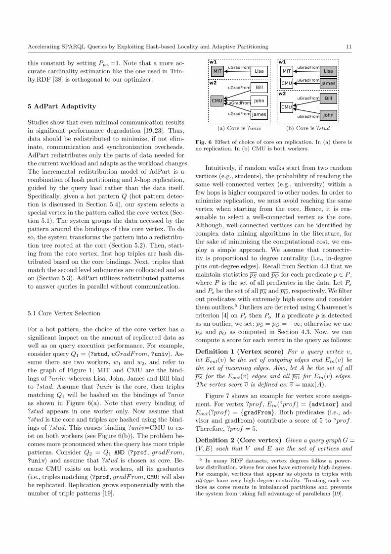
5.1 Core Vertex Selection

For a hot pattern, the choice of the core vertex has asignificant impact on the amount of replicated data as

well as on query execution performance. For example,

consider query Q1 = 〈?stud, uGradFrom, ?univ〉. As-sume there are two workers, w1 and w2, and refer to

the graph of Figure 1; MIT and CMU are the bind-

ings of ?univ, whereas Lisa, John, James and Bill bind

to ?stud. Assume that ?univ is the core, then triplesmatching Q1 will be hashed on the bindings of ?univ

as shown in Figure 6(a). Note that every binding of

?stud appears in one worker only. Now assume that?stud is the core and triples are hashed using the bind-

ings of ?stud. This causes binding ?univ=CMU to ex-

ist on both workers (see Figure 6(b)). The problem be-comes more pronounced when the query has more triple

patterns. Consider Q2 = Q1 AND 〈?prof, gradFrom,

?univ〉 and assume that ?stud is chosen as core. Be-

cause CMU exists on both workers, all its graduates(i.e., triples matching 〈?prof, gradFrom, CMU〉 will also

be replicated. Replication grows exponentially with the

number of triple patterns [19].

(a) Core is ?univ (b) Core is ?stud

Fig. 6 Effect of choice of core on replication. In (a) there isno replication. In (b) CMU is both workers.

Intuitively, if random walks start from two random

vertices (e.g., students), the probability of reaching the

same well-connected vertex (e.g., university) within afew hops is higher compared to other nodes. In order to

minimize replication, we must avoid reaching the same

vertex when starting from the core. Hence, it is rea-sonable to select a well-connected vertex as the core.

Although, well-connected vertices can be identified by

complex data mining algorithms in the literature, for

the sake of minimizing the computational cost, we em-ploy a simple approach. We assume that connectiv-

ity is proportional to degree centrality (i.e., in-degree

plus out-degree edges). Recall from Section 4.3 that wemaintain statistics pS and pO for each predicate p ∈ P ,

where P is the set of all predicates in the data. Let Ps

and Po be the set of all pS and pO, respectively. We filterout predicates with extremely high scores and consider

them outliers.5 Outliers are detected using Chauvenet’s

criterion [4] on Ps then Po. If a predicate p is detected

as an outlier, we set: pS = pO = −∞; otherwise we usepS and pO as computed in Section 4.3. Now, we can

compute a score for each vertex in the query as follows:

Definition 1 (Vertex score) For a query vertex v,let Eout(v) be the set of outgoing edges and Ein(v) be

the set of incoming edges. Also, let A be the set of all

pS for the Eout(v) edges and all pO for Ein(v) edges.

The vertex score v is defined as: v = max(A).

Figure 7 shows an example for vertex score assign-

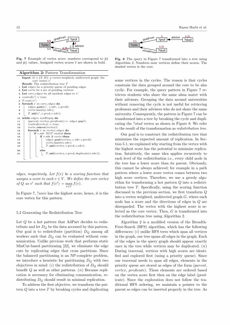
ment. For vertex ?prof , Ein(?prof) = {advisor} and

Eout(?prof) = {gradFrom}. Both predicates (i.e., ad-visor and gradFrom) contribute a score of 5 to ?prof .

Therefore, ?prof = 5.

Definition 2 (Core vertex) Given a query graph G =

(V,E) such that V and E are the set of vertices and

5 In many RDF datasets, vertex degrees follow a power-law distribution, where few ones have extremely high degrees.For example, vertices that appear as objects in triples withrdf:type have very high degree centrality. Treating such ver-tices as cores results in imbalanced partitions and preventsthe system from taking full advantage of parallelism [19].

12 Razen Harbi et al.

Fig. 7 Example of vertex score: numbers correspond to pSand pO values. Assigned vertex scores v are shown in bold.

Algorithm 2: Pattern TransformationInput: G = {V,E}; a vertex-weighted, undirected graph, the

core vertex v′

Result: The redistribution tree T1 Let edges be a priority queue of pending edges2 Let verts be a set of pending vertices

3 Let core edges be all incident edges to v′

4 visited[v′] = true;

5 T.root=v′;6 foreach e in core edges do7 edges.push(v′, e.nbr, e.pred);8 verts.insert(e.nbr);

9 T.add(v′, e.pred, e.nbr);

10 while edges notEmpty do11 (parent, vertex, predicate)← edges.pop();12 visited[vertex] = true;13 verts.remove(vertex);14 foreach e in vertex.edges do15 if e.nbr NOT visited then16 if e.nbr /∈ verts then17 edges.push(vertex, e.nbr, e.pred);18 verts.insert(e.nbr);19 T.add(vertex, e.pred, e.nbr);

20 else21 T.add(vertex, e.pred, duplicate(e.nbr));

edges, respectively. Let f(v) be a scoring function that

assigns a score to each v ∈ V . We define the core vertex

of Q as v′ such that f(v′) = maxv∈V

f(v).

In Figure 7, ?univ has the highest score, hence, it is thecore vertex for this pattern.

5.2 Generating the Redistribution Tree

Let Q be a hot pattern that AdPart decides to redis-tribute and let DQ be the data accessed by this pattern.

Our goal is to redistribute (partition) DQ among all

workers such that DQ can be evaluated without com-munication. Unlike previous work that performs static

MinCut-based partitioning [22], we eliminate the edge

cuts by replicating edges that cross partitions. Since

the balanced partitioning is an NP-complete problem,we introduce a heuristic for partitioning DQ with two

objectives in mind: (i) the redistribution of DQ should

benefit Q as well as other patterns. (ii) Because repli-cation is necessary for eliminating communication, re-

distributing DQ should result in minimal replication.

To address the first objective, we transform the pat-

tern Q into a tree T by breaking cycles and duplicating

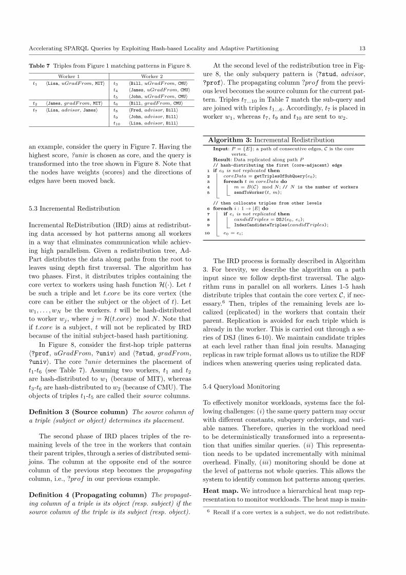
Fig. 8 The query in Figure 7 transformed into a tree usingAlgorithm 2. Numbers near vertices define their scores. Theshaded vertex is the core.

some vertices in the cycles. The reason is that cyclesconstrain the data grouped around the core to be also

cyclic. For example, the query pattern in Figure 7 re-

trieves students who share the same alma mater with

their advisors. Grouping the data around universitieswithout removing the cycle is not useful for retrieving

professors and their advisees who do not share the same

university. Consequently, the pattern in Figure 7 can betransformed into a tree by breaking the cycle and dupli-

cating the ?stud vertex as shown in Figure 8. We refer

to the result of the transformation as redistribution tree.

Our goal is to construct the redistribution tree that

minimizes the expected amount of replication. In Sec-tion 5.1, we explained why starting from the vertex with

the highest score has the potential to minimize replica-

tion. Intuitively, the same idea applies recursively toeach level of the redistribution i.e., every child node in

the tree has a lower score than its parent. Obviously,

this cannot be always achieved; for example in a pathpattern where a lower score vertex comes between two

high score vertices. Therefore, we use a greedy algo-

rithm for transforming a hot pattern Q into a redistri-

bution tree T . Specifically, using the scoring functiondiscussed in the previous section, we first transform Q

into a vertex weighted, undirected graph G, where each

node has a score and the directions of edges in Q aredisregarded. The vertex with the highest score is se-

lected as the core vertex. Then, G is transformed into

the redistribution tree using Algorithm 2.

Algorithm 2 is a modified version of the Breadth-

First-Search (BFS) algorithm, which has the followingdifferences: (i) unlike BFS trees which span all vertices

in the graph, our tree spans all edges in the graph. Each

of the edges in the query graph should appear exactlyonce in the tree while vertices may be duplicated. (ii)

During traversal, vertices with high scores are identi-

fied and explored first (using a priority queue). Sinceour traversal needs to span all edges, elements in the

priority queue are stored as edges of the form (parent,

vertex, predicate). These elements are ordered based

on the vertex score first then on the edge label (pred-icate). Since the exploration does not follow the tra-

ditional BFS ordering, we maintain a pointer to the

parent so edges can be inserted properly in the tree. As

Accelerating SPARQL Queries by Exploiting Hash-based Locality and Adaptive Partitioning 13

Table 7 Triples from Figure 1 matching patterns in Figure 8.

Worker 1 Worker 2

t1 〈Lisa, uGradFrom, MIT〉 t3 〈Bill, uGradFrom, CMU〉

t4 〈James, uGradFrom, CMU〉

t5 〈John, uGradFrom, CMU〉

t2 〈James, gradFrom, MIT〉 t6 〈Bill, gradFrom, CMU〉

t7 〈Lisa, advisor, James〉 t8 〈Fred, advisor, Bill〉

t9 〈John, advisor, Bill〉

t10 〈Lisa, advisor, Bill〉

an example, consider the query in Figure 7. Having the

highest score, ?univ is chosen as core, and the query is

transformed into the tree shown in Figure 8. Note thatthe nodes have weights (scores) and the directions of

edges have been moved back.

5.3 Incremental Redistribution

Incremental ReDistribution (IRD) aims at redistribut-ing data accessed by hot patterns among all workers

in a way that eliminates communication while achiev-

ing high parallelism. Given a redistribution tree, Ad-Part distributes the data along paths from the root to

leaves using depth first traversal. The algorithm has

two phases. First, it distributes triples containing the

core vertex to workers using hash function H(·). Let tbe such a triple and let t.core be its core vertex (the

core can be either the subject or the object of t). Let

w1, . . . , wN be the workers. t will be hash-distributedto worker wj , where j = H(t.core) mod N . Note that

if t.core is a subject, t will not be replicated by IRD

because of the initial subject-based hash partitioning.

In Figure 8, consider the first-hop triple patterns〈?prof, uGradFrom, ?univ〉 and 〈?stud, gradFrom,

?univ〉. The core ?univ determines the placement of

t1-t6 (see Table 7). Assuming two workers, t1 and t2are hash-distributed to w1 (because of MIT), whereast3-t6 are hash-distributed to w2 (because of CMU). The

objects of triples t1-t5 are called their source columns.

Definition 3 (Source column) The source column ofa triple (subject or object) determines its placement.

The second phase of IRD places triples of the re-

maining levels of the tree in the workers that containtheir parent triples, through a series of distributed semi-

joins. The column at the opposite end of the source

column of the previous step becomes the propagatingcolumn, i.e., ?prof in our previous example.

Definition 4 (Propagating column) The propagat-

ing column of a triple is its object (resp. subject) if the

source column of the triple is its subject (resp. object).

At the second level of the redistribution tree in Fig-

ure 8, the only subquery pattern is 〈?stud, advisor,?prof〉. The propagating column ?prof from the previ-

ous level becomes the source column for the current pat-

tern. Triples t7...10 in Table 7 match the sub-query andare joined with triples t1...6. Accordingly, t7 is placed in

worker w1, whereas t7, t9 and t10 are sent to w2.

Algorithm 3: Incremental RedistributionInput: P = {E}; a path of consecutive edges, C is the core

vertex.Result: Data replicated along path P// hash-distributing the first (core-adjacent) edge

1 if e0 is not replicated then2 coreData = getTriplesOfSubQuery(e0);3 foreach t in coreData do4 m = B(C) mod N ; // N is the number of workers5 sendToWorker(t, m);

// then collocate triples from other levels6 foreach i : 1→ |E| do7 if ei is not replicated then8 candidTriples = DSJ(e0, ei);9 IndexCandidateTriples(candidTriples);

10 e0 = ei;

The IRD process is formally described in Algorithm3. For brevity, we describe the algorithm on a path

input since we follow depth-first traversal. The algo-

rithm runs in parallel on all workers. Lines 1-5 hashdistribute triples that contain the core vertex C, if nec-

essary.6 Then, triples of the remaining levels are lo-

calized (replicated) in the workers that contain theirparent. Replication is avoided for each triple which is

already in the worker. This is carried out through a se-

ries of DSJ (lines 6-10). We maintain candidate triples

at each level rather than final join results. Managingreplicas in raw triple format allows us to utilize the RDF

indices when answering queries using replicated data.

5.4 Queryload Monitoring

To effectively monitor workloads, systems face the fol-

lowing challenges: (i) the same query pattern may occurwith different constants, subquery orderings, and vari-

able names. Therefore, queries in the workload need

to be deterministically transformed into a representa-tion that unifies similar queries. (ii) This representa-

tion needs to be updated incrementally with minimal

overhead. Finally, (iii) monitoring should be done at

the level of patterns not whole queries. This allows thesystem to identify common hot patterns among queries.

Heat map. We introduce a hierarchical heat map rep-resentation to monitor workloads. The heat map is main-

6 Recall if a core vertex is a subject, we do not redistribute.

14 Razen Harbi et al.

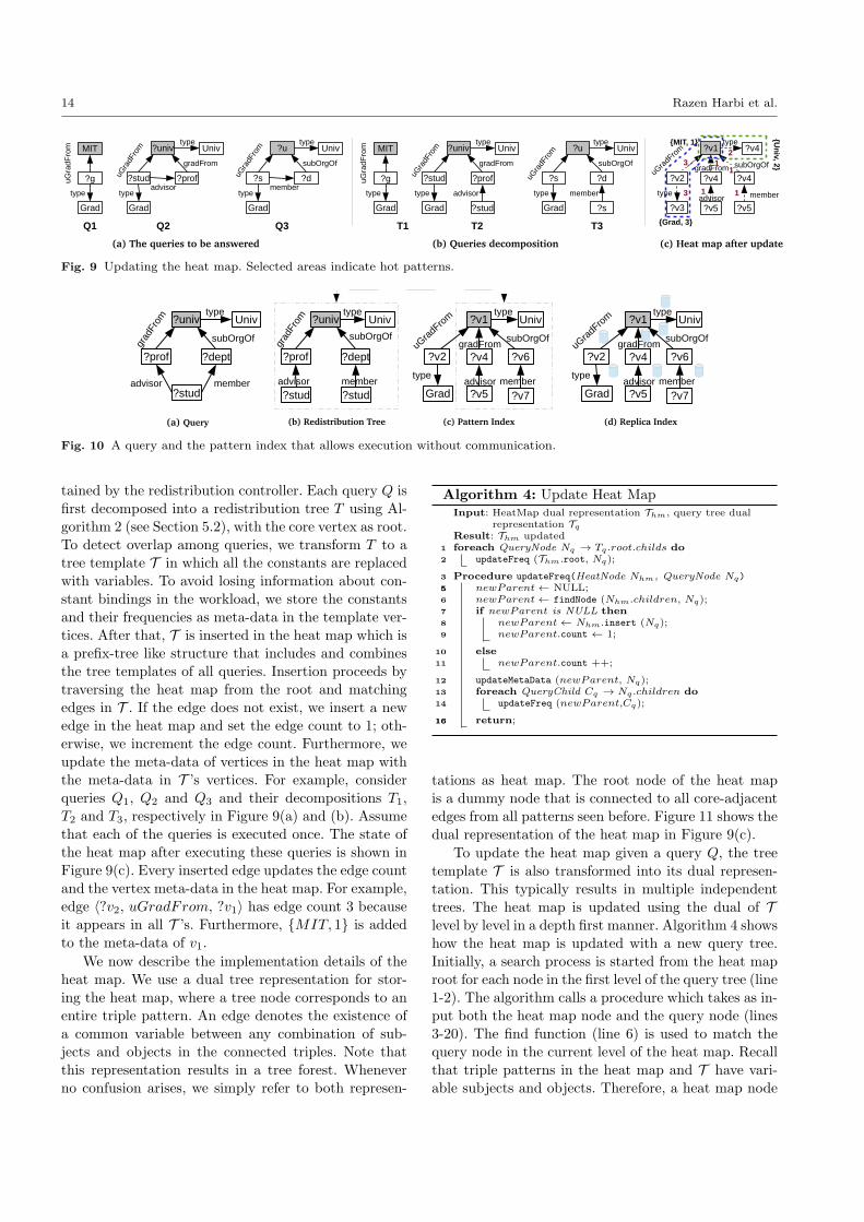
Fig. 9 Updating the heat map. Selected areas indicate hot patterns.

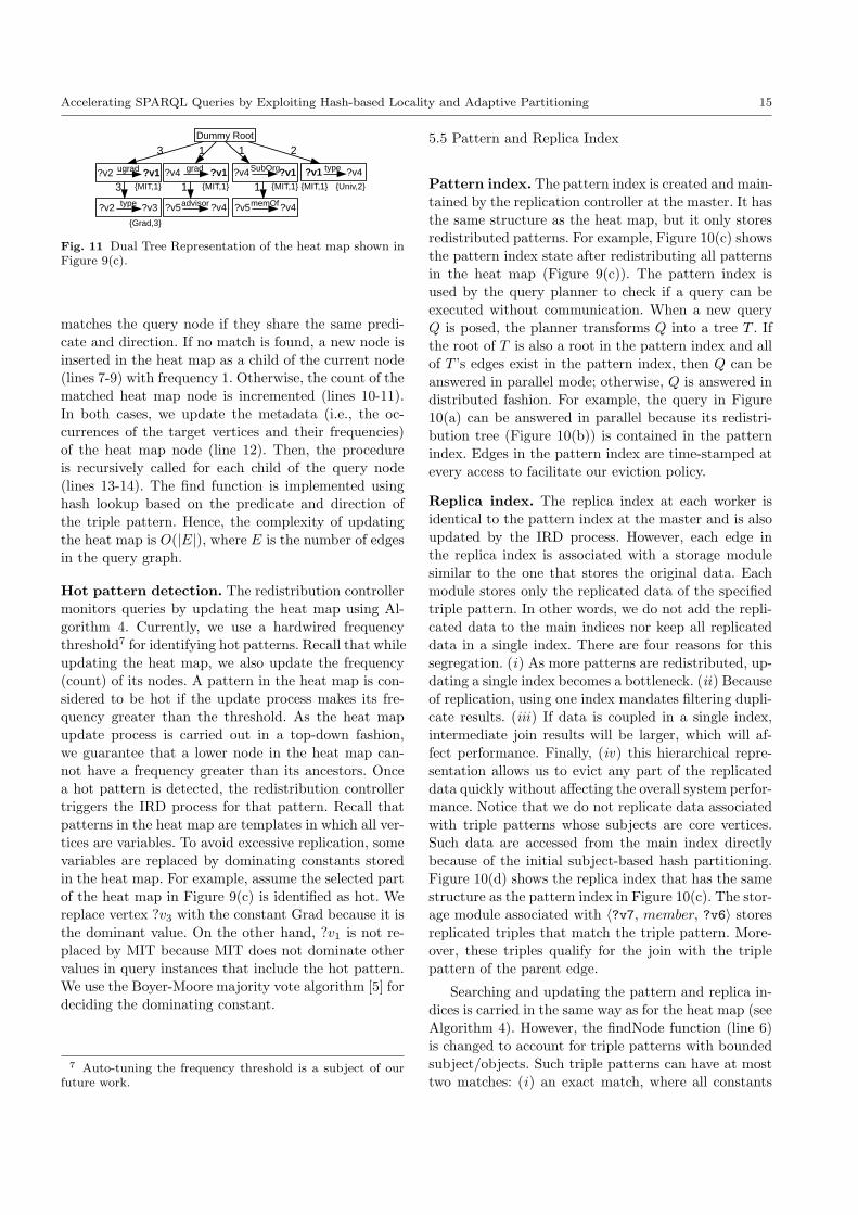
Fig. 10 A query and the pattern index that allows execution without communication.

tained by the redistribution controller. Each query Q isfirst decomposed into a redistribution tree T using Al-

gorithm 2 (see Section 5.2), with the core vertex as root.

To detect overlap among queries, we transform T to atree template T in which all the constants are replaced

with variables. To avoid losing information about con-

stant bindings in the workload, we store the constants

and their frequencies as meta-data in the template ver-tices. After that, T is inserted in the heat map which is

a prefix-tree like structure that includes and combines

the tree templates of all queries. Insertion proceeds bytraversing the heat map from the root and matching

edges in T . If the edge does not exist, we insert a new

edge in the heat map and set the edge count to 1; oth-erwise, we increment the edge count. Furthermore, we

update the meta-data of vertices in the heat map with

the meta-data in T ’s vertices. For example, consider

queries Q1, Q2 and Q3 and their decompositions T1,T2 and T3, respectively in Figure 9(a) and (b). Assume

that each of the queries is executed once. The state of

the heat map after executing these queries is shown inFigure 9(c). Every inserted edge updates the edge count

and the vertex meta-data in the heat map. For example,

edge 〈?v2, uGradFrom, ?v1〉 has edge count 3 becauseit appears in all T ’s. Furthermore, {MIT, 1} is added

to the meta-data of v1.

We now describe the implementation details of theheat map. We use a dual tree representation for stor-

ing the heat map, where a tree node corresponds to an

entire triple pattern. An edge denotes the existence of

a common variable between any combination of sub-jects and objects in the connected triples. Note that

this representation results in a tree forest. Whenever

no confusion arises, we simply refer to both represen-

Algorithm 4: Update Heat MapInput: HeatMap dual representation Thm, query tree dual

representation TqResult: Thm updated

1 foreach QueryNode Nq → Tq.root.childs do2 updateFreq (Thm.root, Nq);

3 Procedure updateFreq(HeatNode Nhm, QueryNode Nq)55 newParent← NULL;6 newParent← findNode (Nhm.children, Nq);7 if newParent is NULL then8 newParent← Nhm.insert (Nq);9 newParent.count ← 1;

10 else11 newParent.count ++;

12 updateMetaData (newParent, Nq);13 foreach QueryChild Cq → Nq.children do14 updateFreq (newParent,Cq);

1616 return;

tations as heat map. The root node of the heat mapis a dummy node that is connected to all core-adjacent

edges from all patterns seen before. Figure 11 shows the

dual representation of the heat map in Figure 9(c).

To update the heat map given a query Q, the treetemplate T is also transformed into its dual represen-

tation. This typically results in multiple independent

trees. The heat map is updated using the dual of Tlevel by level in a depth first manner. Algorithm 4 shows

how the heat map is updated with a new query tree.

Initially, a search process is started from the heat maproot for each node in the first level of the query tree (line

1-2). The algorithm calls a procedure which takes as in-

put both the heat map node and the query node (lines

3-20). The find function (line 6) is used to match thequery node in the current level of the heat map. Recall

that triple patterns in the heat map and T have vari-

able subjects and objects. Therefore, a heat map node

Accelerating SPARQL Queries by Exploiting Hash-based Locality and Adaptive Partitioning 15

Fig. 11 Dual Tree Representation of the heat map shown inFigure 9(c).

matches the query node if they share the same predi-

cate and direction. If no match is found, a new node is

inserted in the heat map as a child of the current node(lines 7-9) with frequency 1. Otherwise, the count of the

matched heat map node is incremented (lines 10-11).

In both cases, we update the metadata (i.e., the oc-

currences of the target vertices and their frequencies)of the heat map node (line 12). Then, the procedure

is recursively called for each child of the query node

(lines 13-14). The find function is implemented usinghash lookup based on the predicate and direction of

the triple pattern. Hence, the complexity of updating

the heat map is O(|E|), where E is the number of edgesin the query graph.

Hot pattern detection. The redistribution controller

monitors queries by updating the heat map using Al-gorithm 4. Currently, we use a hardwired frequency

threshold7 for identifying hot patterns. Recall that while

updating the heat map, we also update the frequency(count) of its nodes. A pattern in the heat map is con-

sidered to be hot if the update process makes its fre-

quency greater than the threshold. As the heat mapupdate process is carried out in a top-down fashion,

we guarantee that a lower node in the heat map can-

not have a frequency greater than its ancestors. Once

a hot pattern is detected, the redistribution controllertriggers the IRD process for that pattern. Recall that

patterns in the heat map are templates in which all ver-

tices are variables. To avoid excessive replication, somevariables are replaced by dominating constants stored

in the heat map. For example, assume the selected part

of the heat map in Figure 9(c) is identified as hot. Wereplace vertex ?v3 with the constant Grad because it is

the dominant value. On the other hand, ?v1 is not re-

placed by MIT because MIT does not dominate other

values in query instances that include the hot pattern.We use the Boyer-Moore majority vote algorithm [5] for

deciding the dominating constant.

7 Auto-tuning the frequency threshold is a subject of ourfuture work.

5.5 Pattern and Replica Index

Pattern index. The pattern index is created and main-tained by the replication controller at the master. It has

the same structure as the heat map, but it only stores

redistributed patterns. For example, Figure 10(c) shows

the pattern index state after redistributing all patternsin the heat map (Figure 9(c)). The pattern index is

used by the query planner to check if a query can be

executed without communication. When a new queryQ is posed, the planner transforms Q into a tree T . If

the root of T is also a root in the pattern index and all

of T ’s edges exist in the pattern index, then Q can beanswered in parallel mode; otherwise, Q is answered in

distributed fashion. For example, the query in Figure

10(a) can be answered in parallel because its redistri-

bution tree (Figure 10(b)) is contained in the patternindex. Edges in the pattern index are time-stamped at

every access to facilitate our eviction policy.

Replica index. The replica index at each worker is

identical to the pattern index at the master and is also

updated by the IRD process. However, each edge inthe replica index is associated with a storage module

similar to the one that stores the original data. Each

module stores only the replicated data of the specifiedtriple pattern. In other words, we do not add the repli-

cated data to the main indices nor keep all replicated

data in a single index. There are four reasons for this

segregation. (i) As more patterns are redistributed, up-dating a single index becomes a bottleneck. (ii) Because

of replication, using one index mandates filtering dupli-

cate results. (iii) If data is coupled in a single index,intermediate join results will be larger, which will af-

fect performance. Finally, (iv) this hierarchical repre-

sentation allows us to evict any part of the replicateddata quickly without affecting the overall system perfor-

mance. Notice that we do not replicate data associated

with triple patterns whose subjects are core vertices.

Such data are accessed from the main index directlybecause of the initial subject-based hash partitioning.

Figure 10(d) shows the replica index that has the same

structure as the pattern index in Figure 10(c). The stor-age module associated with 〈?v7, member, ?v6〉 stores

replicated triples that match the triple pattern. More-

over, these triples qualify for the join with the triplepattern of the parent edge.

Searching and updating the pattern and replica in-

dices is carried in the same way as for the heat map (see

Algorithm 4). However, the findNode function (line 6)is changed to account for triple patterns with bounded

subject/objects. Such triple patterns can have at most

two matches: (i) an exact match, where all constants

16 Razen Harbi et al.

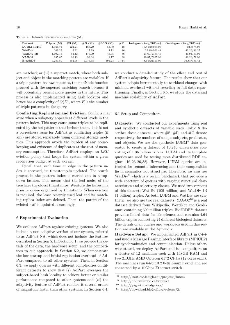
Table 8 Datasets Statistics in millions (M)

Dataset Triples (M) #S (M) #O (M) #S∩O (M) #P Indegree (Avg/StDev) Outdegree (Avg/StDev)

LUBM-10240 1,366.71 222.21 165.29 51.00 18 16.54/26000.00 12.30/5.97

WatDiv 109.23 5.21 17.93 4.72 86 22.49/960.44 42.20/89.25

WatDiv-1B 1,092.16 52.12 179.09 46.95 86 23.69/2783.40 41.91/89.05

YAGO2 295.85 10.12 52.34 1.77 98 10.87/5925.90 56.20/71.96

Bio2RDF 4,287.59 552.08 1,075.58 491.73 1,714 8.64/21110.00 16.83/195.44

are matched; or (ii) a superset match, where both sub-ject and object in the matching pattern are variables. If

a triple pattern has two matches, the findNode function

proceed with the superset matching branch because itwill potentially benefit more queries in the future. This

process is also implemented using hash lookups and

hence has a complexity of O(E), where E is the number

of triple patterns in the query.

Conflicting Replication and Eviction. Conflicts may

arise when a subquery appears at different levels in thepattern index. This may cause some triples to be repli-

cated by the hot patterns that include them. This is not

a correctness issue for AdPart as conflicting triples (ifany) are stored separately using different storage mod-

ules. This approach avoids the burden of any house-

keeping and existence of duplicates at the cost of mem-ory consumption. Therefore, AdPart employs an LRU

eviction policy that keeps the system within a given

replication budget at each worker.

Recall that, each time an edge in the pattern in-dex is accessed, its timestamp is updated. The search

process in the pattern index is carried out in a top-

down fashion. This means that the leaf nodes of thetree have the oldest timestamps. We store the leaves in a

priority queue organized by timestamp. When eviction

is required, the least recently used leaf and its match-ing replica index are deleted. Then, the parent of the

evicted leaf is updated accordingly.

6 Experimental Evaluation

We evaluate AdPart against existing systems. We alsoinclude a non-adaptive version of our system, referred

to as AdPart-NA, which does not include the features

described in Section 5. In Section 6.1, we provide the de-tails of the data, the hardware setup, and the competi-

tors to our approach. In Section 6.2, we demonstrate

the low startup and initial replication overhead of Ad-Part compared to all other systems. Then, in Section

6.3, we apply queries with different complexities on dif-

ferent datasets to show that (i) AdPart leverages the

subject-based hash locality to achieve better or similarperformance compared to other systems and (ii) the

adaptivity feature of AdPart renders it several orders

of magnitude faster than other systems. In Section 6.4,

we conduct a detailed study of the effect and cost ofAdPart’s adaptivity feature. The results show that our

system adapts incrementally to workload changes with

minimal overhead without resorting to full data repar-titioning. Finally, in Section 6.5, we study the data and

machine scalability of AdPart.

6.1 Setup and Competitors

Datasets: We conducted our experiments using real

and synthetic datasets of variable sizes. Table 8 de-scribes these datasets, where #S, #P, and #O denote

respectively the numbers of unique subjects, predicates,

and objects. We use the synthetic LUBM8 data gen-erator to create a dataset of 10,240 universities con-

sisting of 1.36 billion triples. LUBM and its template

queries are used for testing most distributed RDF en-

gines [16,23,26,38]. However, LUBM queries are in-tended for semantic inferencing and their complexities

lie in semantics not structure. Therefore, we also use

WatDiv9 which is a recent benchmark that provides awide spectrum of queries with varying structural char-

acteristics and selectivity classes. We used two versions

of this dataset: WatDiv (109 million) and WatDiv-1B(1 billion) triples. As both LUBM and WatDiv are syn-

thetic, we also use two real datasets. YAGO210 is a real

dataset derived from Wikipedia, WordNet and GeoN-

ames containing 300 million triples. Bio2RDF11 datasetprovides linked data for life sciences and contains 4.64

billion triples connecting 24 different biological datasets.

The details of all queries and workloads used in this sec-tion are available in the Appendix.

Hardware Setup: We implemented AdPart in C++and used a Message Passing Interface library (MPICH2)

for synchronization and communication. Unless other-

wise stated, we deploy AdPart and its competitors ona cluster of 12 machines each with 148GB RAM and

two 2.1GHz AMD Opteron 6172 CPUs (12 cores each).

The machines run 64-bit 3.2.0-38 Linux Kernel and areconnected by a 10Gbps Ethernet switch.

8 http://swat.cse.lehigh.edu/projects/lubm/9 http://db.uwaterloo.ca/watdiv/

10 http://yago-knowledge.org/11 http://download.bio2rdf.org/release/2/

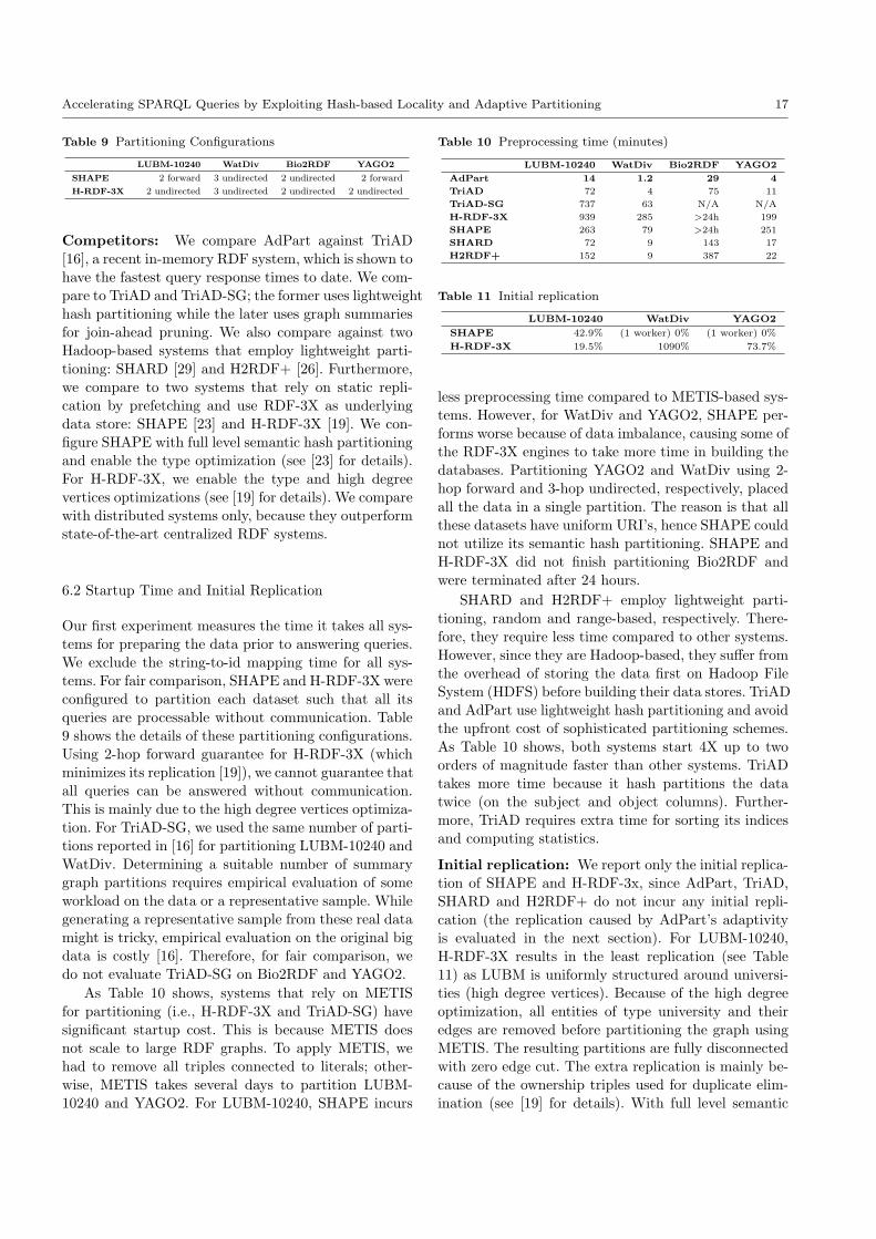
Accelerating SPARQL Queries by Exploiting Hash-based Locality and Adaptive Partitioning 17

Table 9 Partitioning Configurations

LUBM-10240 WatDiv Bio2RDF YAGO2

SHAPE 2 forward 3 undirected 2 undirected 2 forward

H-RDF-3X 2 undirected 3 undirected 2 undirected 2 undirected

Competitors: We compare AdPart against TriAD

[16], a recent in-memory RDF system, which is shown to

have the fastest query response times to date. We com-pare to TriAD and TriAD-SG; the former uses lightweight

hash partitioning while the later uses graph summaries

for join-ahead pruning. We also compare against twoHadoop-based systems that employ lightweight parti-

tioning: SHARD [29] and H2RDF+ [26]. Furthermore,

we compare to two systems that rely on static repli-

cation by prefetching and use RDF-3X as underlyingdata store: SHAPE [23] and H-RDF-3X [19]. We con-

figure SHAPE with full level semantic hash partitioning

and enable the type optimization (see [23] for details).For H-RDF-3X, we enable the type and high degree

vertices optimizations (see [19] for details). We compare

with distributed systems only, because they outperformstate-of-the-art centralized RDF systems.

6.2 Startup Time and Initial Replication

Our first experiment measures the time it takes all sys-tems for preparing the data prior to answering queries.

We exclude the string-to-id mapping time for all sys-

tems. For fair comparison, SHAPE and H-RDF-3X were

configured to partition each dataset such that all itsqueries are processable without communication. Table

9 shows the details of these partitioning configurations.

Using 2-hop forward guarantee for H-RDF-3X (whichminimizes its replication [19]), we cannot guarantee that

all queries can be answered without communication.

This is mainly due to the high degree vertices optimiza-tion. For TriAD-SG, we used the same number of parti-

tions reported in [16] for partitioning LUBM-10240 and

WatDiv. Determining a suitable number of summary

graph partitions requires empirical evaluation of someworkload on the data or a representative sample. While

generating a representative sample from these real data

might is tricky, empirical evaluation on the original bigdata is costly [16]. Therefore, for fair comparison, we

do not evaluate TriAD-SG on Bio2RDF and YAGO2.

As Table 10 shows, systems that rely on METIS

for partitioning (i.e., H-RDF-3X and TriAD-SG) have

significant startup cost. This is because METIS does

not scale to large RDF graphs. To apply METIS, wehad to remove all triples connected to literals; other-

wise, METIS takes several days to partition LUBM-

10240 and YAGO2. For LUBM-10240, SHAPE incurs

Table 10 Preprocessing time (minutes)

LUBM-10240 WatDiv Bio2RDF YAGO2

AdPart 14 1.2 29 4

TriAD 72 4 75 11

TriAD-SG 737 63 N/A N/A

H-RDF-3X 939 285 >24h 199

SHAPE 263 79 >24h 251

SHARD 72 9 143 17

H2RDF+ 152 9 387 22

Table 11 Initial replication

LUBM-10240 WatDiv YAGO2

SHAPE 42.9% (1 worker) 0% (1 worker) 0%

H-RDF-3X 19.5% 1090% 73.7%

less preprocessing time compared to METIS-based sys-

tems. However, for WatDiv and YAGO2, SHAPE per-forms worse because of data imbalance, causing some of

the RDF-3X engines to take more time in building the

databases. Partitioning YAGO2 and WatDiv using 2-

hop forward and 3-hop undirected, respectively, placedall the data in a single partition. The reason is that all

these datasets have uniform URI’s, hence SHAPE could

not utilize its semantic hash partitioning. SHAPE andH-RDF-3X did not finish partitioning Bio2RDF and

were terminated after 24 hours.

SHARD and H2RDF+ employ lightweight parti-

tioning, random and range-based, respectively. There-

fore, they require less time compared to other systems.

However, since they are Hadoop-based, they suffer fromthe overhead of storing the data first on Hadoop File

System (HDFS) before building their data stores. TriAD

and AdPart use lightweight hash partitioning and avoidthe upfront cost of sophisticated partitioning schemes.

As Table 10 shows, both systems start 4X up to two

orders of magnitude faster than other systems. TriADtakes more time because it hash partitions the data

twice (on the subject and object columns). Further-

more, TriAD requires extra time for sorting its indices

and computing statistics.

Initial replication: We report only the initial replica-tion of SHAPE and H-RDF-3x, since AdPart, TriAD,

SHARD and H2RDF+ do not incur any initial repli-

cation (the replication caused by AdPart’s adaptivityis evaluated in the next section). For LUBM-10240,

H-RDF-3X results in the least replication (see Table

11) as LUBM is uniformly structured around universi-ties (high degree vertices). Because of the high degree

optimization, all entities of type university and their

edges are removed before partitioning the graph using

METIS. The resulting partitions are fully disconnectedwith zero edge cut. The extra replication is mainly be-

cause of the ownership triples used for duplicate elim-

ination (see [19] for details). With full level semantic

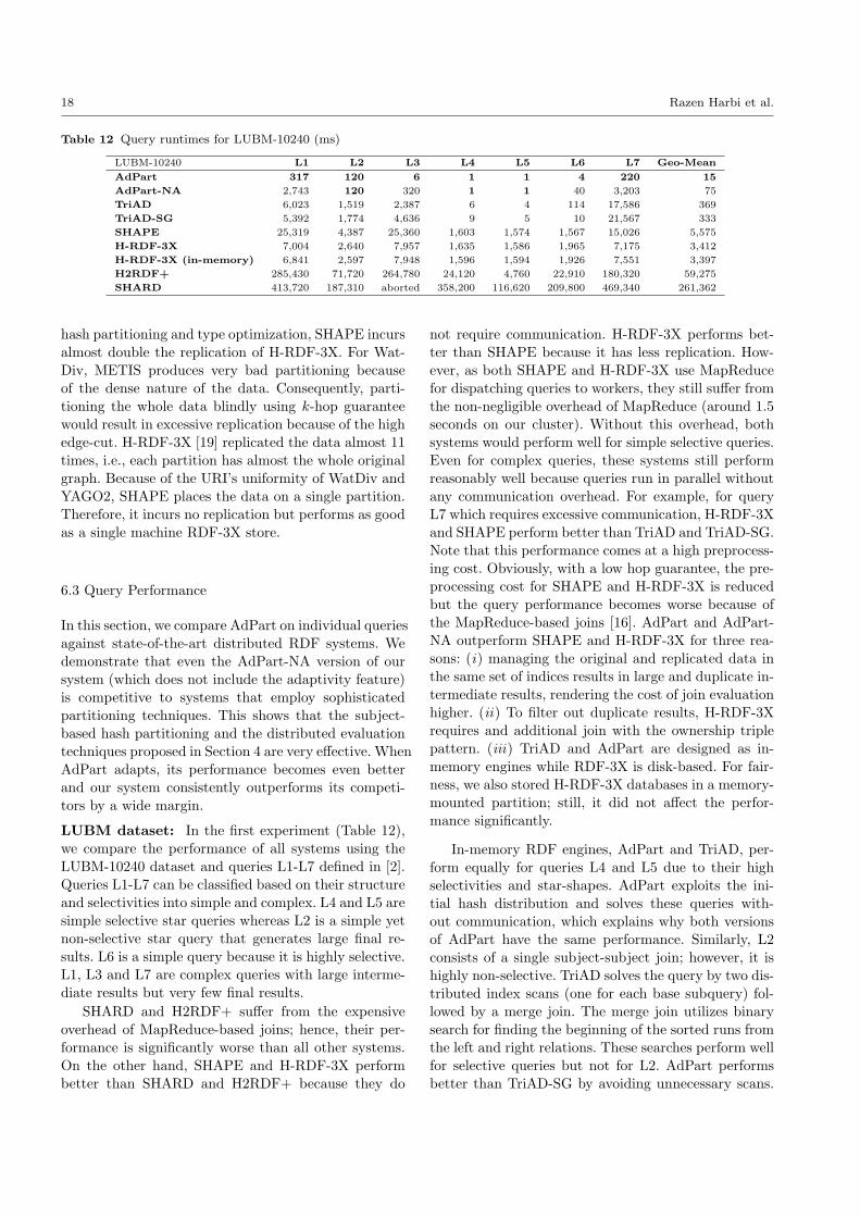
18 Razen Harbi et al.

Table 12 Query runtimes for LUBM-10240 (ms)

LUBM-10240 L1 L2 L3 L4 L5 L6 L7 Geo-Mean

AdPart 317 120 6 1 1 4 220 15

AdPart-NA 2,743 120 320 1 1 40 3,203 75

TriAD 6,023 1,519 2,387 6 4 114 17,586 369

TriAD-SG 5,392 1,774 4,636 9 5 10 21,567 333

SHAPE 25,319 4,387 25,360 1,603 1,574 1,567 15,026 5,575

H-RDF-3X 7,004 2,640 7,957 1,635 1,586 1,965 7,175 3,412

H-RDF-3X (in-memory) 6,841 2,597 7,948 1,596 1,594 1,926 7,551 3,397

H2RDF+ 285,430 71,720 264,780 24,120 4,760 22,910 180,320 59,275

SHARD 413,720 187,310 aborted 358,200 116,620 209,800 469,340 261,362

hash partitioning and type optimization, SHAPE incurs

almost double the replication of H-RDF-3X. For Wat-Div, METIS produces very bad partitioning because

of the dense nature of the data. Consequently, parti-

tioning the whole data blindly using k-hop guarantee

would result in excessive replication because of the highedge-cut. H-RDF-3X [19] replicated the data almost 11

times, i.e., each partition has almost the whole original

graph. Because of the URI’s uniformity of WatDiv andYAGO2, SHAPE places the data on a single partition.

Therefore, it incurs no replication but performs as good

as a single machine RDF-3X store.

6.3 Query Performance

In this section, we compare AdPart on individual queries

against state-of-the-art distributed RDF systems. We

demonstrate that even the AdPart-NA version of oursystem (which does not include the adaptivity feature)

is competitive to systems that employ sophisticated

partitioning techniques. This shows that the subject-based hash partitioning and the distributed evaluation

techniques proposed in Section 4 are very effective. When

AdPart adapts, its performance becomes even betterand our system consistently outperforms its competi-

tors by a wide margin.

LUBM dataset: In the first experiment (Table 12),we compare the performance of all systems using the

LUBM-10240 dataset and queries L1-L7 defined in [2].

Queries L1-L7 can be classified based on their structureand selectivities into simple and complex. L4 and L5 are

simple selective star queries whereas L2 is a simple yet

non-selective star query that generates large final re-

sults. L6 is a simple query because it is highly selective.L1, L3 and L7 are complex queries with large interme-

diate results but very few final results.

SHARD and H2RDF+ suffer from the expensive

overhead of MapReduce-based joins; hence, their per-formance is significantly worse than all other systems.

On the other hand, SHAPE and H-RDF-3X perform

better than SHARD and H2RDF+ because they do

not require communication. H-RDF-3X performs bet-

ter than SHAPE because it has less replication. How-ever, as both SHAPE and H-RDF-3X use MapReduce

for dispatching queries to workers, they still suffer from

the non-negligible overhead of MapReduce (around 1.5

seconds on our cluster). Without this overhead, bothsystems would perform well for simple selective queries.

Even for complex queries, these systems still perform

reasonably well because queries run in parallel withoutany communication overhead. For example, for query

L7 which requires excessive communication, H-RDF-3X

and SHAPE perform better than TriAD and TriAD-SG.Note that this performance comes at a high preprocess-

ing cost. Obviously, with a low hop guarantee, the pre-

processing cost for SHAPE and H-RDF-3X is reduced

but the query performance becomes worse because ofthe MapReduce-based joins [16]. AdPart and AdPart-

NA outperform SHAPE and H-RDF-3X for three rea-

sons: (i) managing the original and replicated data inthe same set of indices results in large and duplicate in-

termediate results, rendering the cost of join evaluation

higher. (ii) To filter out duplicate results, H-RDF-3Xrequires and additional join with the ownership triple

pattern. (iii) TriAD and AdPart are designed as in-

memory engines while RDF-3X is disk-based. For fair-

ness, we also stored H-RDF-3X databases in a memory-mounted partition; still, it did not affect the perfor-

mance significantly.

In-memory RDF engines, AdPart and TriAD, per-form equally for queries L4 and L5 due to their high

selectivities and star-shapes. AdPart exploits the ini-

tial hash distribution and solves these queries with-out communication, which explains why both versions

of AdPart have the same performance. Similarly, L2

consists of a single subject-subject join; however, it ishighly non-selective. TriAD solves the query by two dis-

tributed index scans (one for each base subquery) fol-

lowed by a merge join. The merge join utilizes binary

search for finding the beginning of the sorted runs fromthe left and right relations. These searches perform well

for selective queries but not for L2. AdPart performs

better than TriAD-SG by avoiding unnecessary scans.

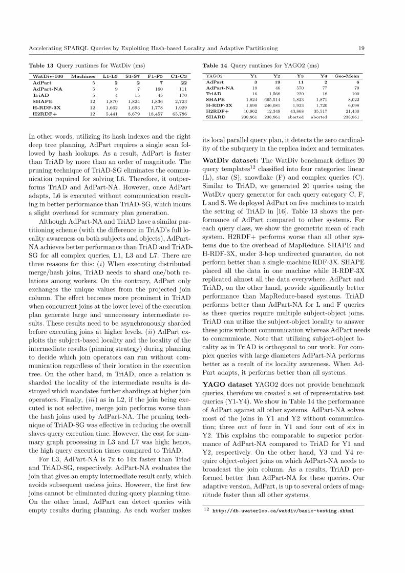
Accelerating SPARQL Queries by Exploiting Hash-based Locality and Adaptive Partitioning 19

Table 13 Query runtimes for WatDiv (ms)

WatDiv-100 Machines L1-L5 S1-S7 F1-F5 C1-C3

AdPart 5 2 2 7 22

AdPart-NA 5 9 7 160 111

TriAD 5 4 15 45 170

SHAPE 12 1,870 1,824 1,836 2,723

H-RDF-3X 12 1,662 1,693 1,778 1,929

H2RDF+ 12 5,441 8,679 18,457 65,786

In other words, utilizing its hash indexes and the right

deep tree planning, AdPart requires a single scan fol-

lowed by hash lookups. As a result, AdPart is fasterthan TriAD by more than an order of magnitude. The

pruning technique of TriAD-SG eliminates the commu-

nication required for solving L6. Therefore, it outper-forms TriAD and AdPart-NA. However, once AdPart

adapts, L6 is executed without communication result-

ing in better performance than TriAD-SG, which incurs

a slight overhead for summary plan generation.

Although AdPart-NA and TriAD have a similar par-titioning scheme (with the difference in TriAD’s full lo-

cality awareness on both subjects and objects), AdPart-

NA achieves better performance than TriAD and TriAD-SG for all complex queries, L1, L3 and L7. There are

three reasons for this: (i) When executing distributed

merge/hash joins, TriAD needs to shard one/both re-lations among workers. On the contrary, AdPart only

exchanges the unique values from the projected join

column. The effect becomes more prominent in TriAD

when concurrent joins at the lower level of the executionplan generate large and unnecessary intermediate re-

sults. These results need to be asynchronously sharded

before executing joins at higher levels. (ii) AdPart ex-ploits the subject-based locality and the locality of the

intermediate results (pinning strategy) during planning

to decide which join operators can run without com-munication regardless of their location in the execution

tree. On the other hand, in TriAD, once a relation is

sharded the locality of the intermediate results is de-

stroyed which mandates further shardings at higher joinoperators. Finally, (iii) as in L2, if the join being exe-

cuted is not selective, merge join performs worse than

the hash joins used by AdPart-NA. The pruning tech-nique of TriAD-SG was effective in reducing the overall

slaves query execution time. However, the cost for sum-

mary graph processing in L3 and L7 was high; hence,the high query execution times compared to TriAD.

For L3, AdPart-NA is 7x to 14x faster than Triad

and TriAD-SG, respectively. AdPart-NA evaluates the

join that gives an empty intermediate result early, which

avoids subsequent useless joins. However, the first fewjoins cannot be eliminated during query planning time.

On the other hand, AdPart can detect queries with

empty results during planning. As each worker makes

Table 14 Query runtimes for YAGO2 (ms)

YAGO2 Y1 Y2 Y3 Y4 Geo-Mean

AdPart 3 19 11 2 6

AdPart-NA 19 46 570 77 79

TriAD 16 1,568 220 18 100

SHAPE 1,824 665,514 1,823 1,871 8,022

H-RDF-3X 1,690 246,081 1,933 1,720 6,098

H2RDF+ 10,962 12,349 43,868 35,517 21,430

SHARD 238,861 238,861 aborted aborted 238,861

its local parallel query plan, it detects the zero cardinal-

ity of the subquery in the replica index and terminates.

WatDiv dataset: The WatDiv benchmark defines 20

query templates12 classified into four categories: linear(L), star (S), snowflake (F) and complex queries (C).

Similar to TriAD, we generated 20 queries using the

WatDiv query generator for each query category C, F,L and S. We deployed AdPart on five machines to match

the setting of TriAD in [16]. Table 13 shows the per-

formance of AdPart compared to other systems. Foreach query class, we show the geometric mean of each

system. H2RDF+ performs worse than all other sys-

tems due to the overhead of MapReduce. SHAPE and

H-RDF-3X, under 3-hop undirected guarantee, do notperform better than a single-machine RDF-3X. SHAPE

placed all the data in one machine while H-RDF-3X

replicated almost all the data everywhere. AdPart andTriAD, on the other hand, provide significantly better

performance than MapReduce-based systems. TriAD

performs better than AdPart-NA for L and F queriesas these queries require multiple subject-object joins.

TriAD can utilize the subject-object locality to answer

these joins without communication whereas AdPart needs

to communicate. Note that utilizing subject-object lo-cality as in TriAD is orthogonal to our work. For com-

plex queries with large diameters AdPart-NA performs

better as a result of its locality awareness. When Ad-Part adapts, it performs better than all systems.

YAGO dataset YAGO2 does not provide benchmarkqueries, therefore we created a set of representative test

queries (Y1-Y4). We show in Table 14 the performance

of AdPart against all other systems. AdPart-NA solvesmost of the joins in Y1 and Y2 without communica-

tion; three out of four in Y1 and four out of six in

Y2. This explains the comparable to superior perfor-

mance of AdPart-NA compared to TriAD for Y1 andY2, respectively. On the other hand, Y3 and Y4 re-

quire object-object joins on which AdPart-NA needs to

broadcast the join column. As a results, TriAD per-formed better than AdPart-NA for these queries. Our

adaptive version, AdPart, is up to several orders of mag-

nitude faster than all other systems.

12 http://db.uwaterloo.ca/watdiv/basic-testing.shtml

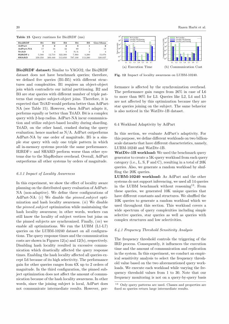
20 Razen Harbi et al.

Table 15 Query runtimes for Bio2RDF (ms)

Bio2RDF B1 B2 B3 B4 B5 Geo-Mean

AdPart 3 2 2 3 1 2

AdPart-NA 17 16 32 89 1 15

TriAD 4 4 5 N/A 2 4

H2RDF+ 5,580 12,710 322,300 7,960 4,280 15,076

SHARD 239,350 309,440 512,850 787,100 112,280 320,027

Bio2RDF dataset: Similar to YAGO2, the Bio2RDF

dataset does not have benchmark queries; therefore,

we defined five queries (B1-B5) with different struc-tures and complexities. B1 requires an object-object

join which contradicts our initial partitioning. B2 and

B3 are star queries with different number of triple pat-terns that require subject-object joins. Therefore, it is

expected that TriAD would perform better than AdPart-

NA (see Table 15). However, when AdPart adapts it,

performs equally or better than TriAD. B4 is a complexquery with 2-hop radius. AdPart-NA incur communica-

tion and utilize subject-based locality during sharding.

TriAD, on the other hand, crashed during the queryevaluation; hence marked as N/A. AdPart outperforms

AdPart-NA by one order of magnitude. B5 is a sim-

ple star query with only one triple pattern in whichall in-memory systems provide the same performance.

H2RDF+ and SHARD perform worse than other sys-

tems due to the MapReduce overhead. Overall, AdPart

outperforms all other systems by orders of magnitude.

6.3.1 Impact of Locality Awareness

In this experiment, we show the effect of locality aware

planning on the distributed query evaluation of AdPart-

NA (non-adaptive). We define three configurations ofAdPart-NA: (i) We disable the pinned subject opti-

mization and hash locality awareness. (ii) We disable

the pinned subject optimization while maintaining thehash locality awareness; in other words, workers can

still know the locality of subject vertices but joins on

the pinned subjects are synchronized. Finally, (iii) we

enable all optimizations. We run the LUBM (L1-L7)queries on the LUBM-10240 dataset on all configura-

tions. The query response times and the communication

costs are shown in Figures 12(a) and 12(b), respectively.Disabling hash locality resulted in excessive commu-

nication which drastically affected the query response

times. Enabling the hash locality affected all queries ex-cept L6 because of its high selectivity. The performance

gain for other queries ranges from 6X up to 2 orders of

magnitude. In the third configuration, the pinned sub-

ject optimization does not affect the amount of commu-nication because of the hash locality awareness. In other

words, since the joining subject is local, AdPart does

not communicate intermediate results. However, per-

10-3

10-2

10-1

100

101

102

103

L1 L2 L3 L4 L5 L6 L7

Tim

e (s

econ

ds)

No-LocalityLocality No-PinningLocality and Pinning

(a) Execution Time

10-6

10-4

10-2

100

102

104

L1 L2 L3 L4 L5 L6 L7

Com

mun

icat

ion

Cos

t (G

iB) No-Locality

Locality No-PinningLocality and Pinning

(b) Communication Cost

Fig. 12 Impact of locality awareness on LUBM-10240.

formance is affected by the synchronization overhead.

The performance gain ranges from 26% in case of L6

to more than 90% for L3. Queries like L2, L4 and L5

are not affected by this optimization because they arestar queries joining on the subject. The same behavior

is also noticed in the WatDiv-1B dataset.

6.4 Workload Adaptivity by AdPart

In this section, we evaluate AdPart’s adaptivity. For

this purpose, we define different workloads on two billion-

scale datasets that have different characteristics, namely,

LUBM-10240 and WatDiv-1B.WatDiv-1B workload: We used the benchmark query

generator to create a 5K-query workload from each query

category (i.e., L, S, F and C), resulting in a total of 20Kqueries. Also, we generate a random workload by shuf-

fling the 20K queries.

LUBM-10240 workload: As AdPart and the othersystems do not support inferencing, we used all 14 queries

in the LUBM benchmark without reasoning13. From

these queries, we generated 10K unique queries that

have different constants and structures. We shuffled the10K queries to generate a random workload which we

used throughout this section. This workload covers a

wide spectrum of query complexities including simpleselective queries, star queries as well as queries with

complex structures and low selectivities.

6.4.1 Frequency Threshold Sensitivity Analysis

The frequency threshold controls the triggering of the

IRD process. Consequently, it influences the executiontime and the amount of communication and replication

in the system. In this experiment, we conduct an empir-

ical sensitivity analysis to select the frequency thresh-old value based on the two aforementioned query work-

loads. We execute each workload while varying the fre-

quency threshold values from 1 to 30. Note that our

frequency monitoring is not on a query-by-query basis

13 Only query patterns are used. Classes and properties arefixed so queries return large intermediate results.

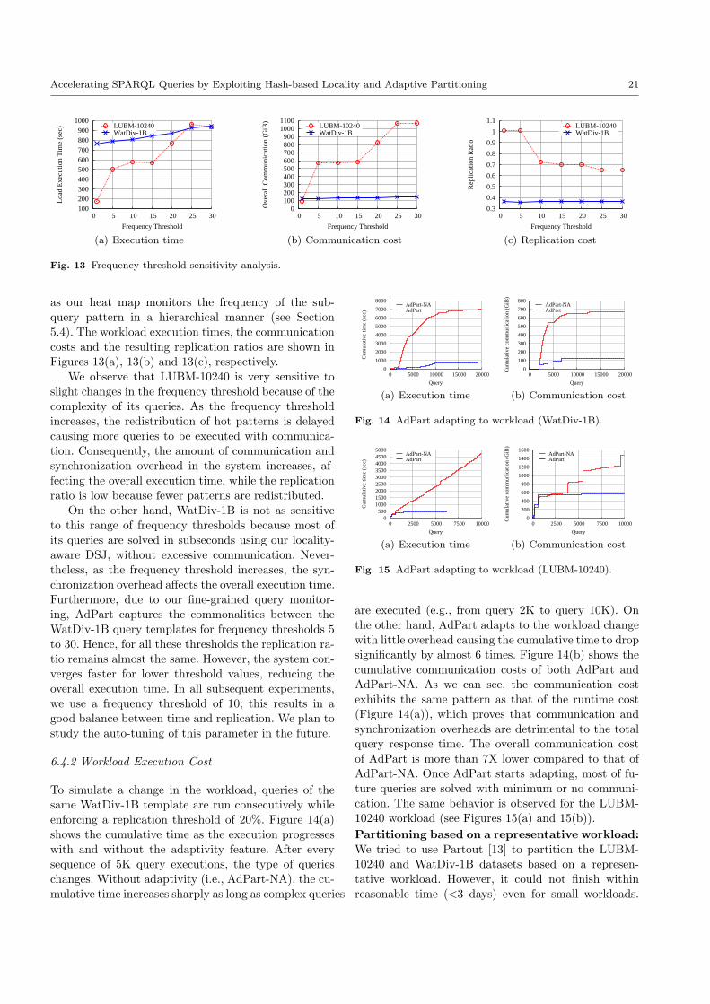
Accelerating SPARQL Queries by Exploiting Hash-based Locality and Adaptive Partitioning 21

100 200 300 400 500 600 700 800 900

1000

0 5 10 15 20 25 30

Loa

d E

xecu

tion

Tim

e (s

ec)

Frequency Threshold

LUBM-10240WatDiv-1B

(a) Execution time

0 100 200 300 400 500 600 700 800 900

1000 1100

0 5 10 15 20 25 30

Ove

rall

Com

mun

icat

ion

(GiB

)

Frequency Threshold

LUBM-10240WatDiv-1B

(b) Communication cost

0.3

0.4

0.5

0.6

0.7

0.8

0.9

1

1.1

0 5 10 15 20 25 30

Rep

licat

ion

Rat

io

Frequency Threshold

LUBM-10240WatDiv-1B

(c) Replication cost

Fig. 13 Frequency threshold sensitivity analysis.

as our heat map monitors the frequency of the sub-query pattern in a hierarchical manner (see Section

5.4). The workload execution times, the communication

costs and the resulting replication ratios are shown inFigures 13(a), 13(b) and 13(c), respectively.

We observe that LUBM-10240 is very sensitive to

slight changes in the frequency threshold because of the

complexity of its queries. As the frequency thresholdincreases, the redistribution of hot patterns is delayed

causing more queries to be executed with communica-

tion. Consequently, the amount of communication andsynchronization overhead in the system increases, af-

fecting the overall execution time, while the replication

ratio is low because fewer patterns are redistributed.On the other hand, WatDiv-1B is not as sensitive

to this range of frequency thresholds because most of

its queries are solved in subseconds using our locality-

aware DSJ, without excessive communication. Never-theless, as the frequency threshold increases, the syn-

chronization overhead affects the overall execution time.

Furthermore, due to our fine-grained query monitor-ing, AdPart captures the commonalities between the

WatDiv-1B query templates for frequency thresholds 5

to 30. Hence, for all these thresholds the replication ra-tio remains almost the same. However, the system con-

verges faster for lower threshold values, reducing the

overall execution time. In all subsequent experiments,

we use a frequency threshold of 10; this results in agood balance between time and replication. We plan to

study the auto-tuning of this parameter in the future.

6.4.2 Workload Execution Cost

To simulate a change in the workload, queries of thesame WatDiv-1B template are run consecutively while

enforcing a replication threshold of 20%. Figure 14(a)

shows the cumulative time as the execution progresses

with and without the adaptivity feature. After everysequence of 5K query executions, the type of queries

changes. Without adaptivity (i.e., AdPart-NA), the cu-

mulative time increases sharply as long as complex queries

0

1000

2000

3000

4000

5000

6000

7000

8000

0 5000 10000 15000 20000

Cum

ulat

ive

time

(sec

)

Query

AdPart-NAAdPart

(a) Execution time

0

100

200

300

400

500

600

700

800

0 5000 10000 15000 20000

Cum

ulat

ive

com

mun

icat

ion

(GiB

)

Query

AdPart-NAAdPart

(b) Communication cost

Fig. 14 AdPart adapting to workload (WatDiv-1B).

0 500

1000 1500 2000 2500 3000 3500 4000 4500 5000

0 2500 5000 7500 10000

Cum

ulat

ive

time

(sec

)

Query

AdPart-NAAdPart

(a) Execution time

0

200

400

600

800

1000

1200

1400

1600

0 2500 5000 7500 10000

Cum

ulat

ive

com

mun

icat

ion

(GiB

)

Query

AdPart-NAAdPart

(b) Communication cost

Fig. 15 AdPart adapting to workload (LUBM-10240).

are executed (e.g., from query 2K to query 10K). Onthe other hand, AdPart adapts to the workload change

with little overhead causing the cumulative time to drop

significantly by almost 6 times. Figure 14(b) shows thecumulative communication costs of both AdPart and

AdPart-NA. As we can see, the communication cost

exhibits the same pattern as that of the runtime cost

(Figure 14(a)), which proves that communication andsynchronization overheads are detrimental to the total

query response time. The overall communication cost

of AdPart is more than 7X lower compared to that ofAdPart-NA. Once AdPart starts adapting, most of fu-

ture queries are solved with minimum or no communi-

cation. The same behavior is observed for the LUBM-10240 workload (see Figures 15(a) and 15(b)).

Partitioning based on a representative workload:

We tried to use Partout [13] to partition the LUBM-10240 and WatDiv-1B datasets based on a represen-

tative workload. However, it could not finish within

reasonable time (<3 days) even for small workloads.

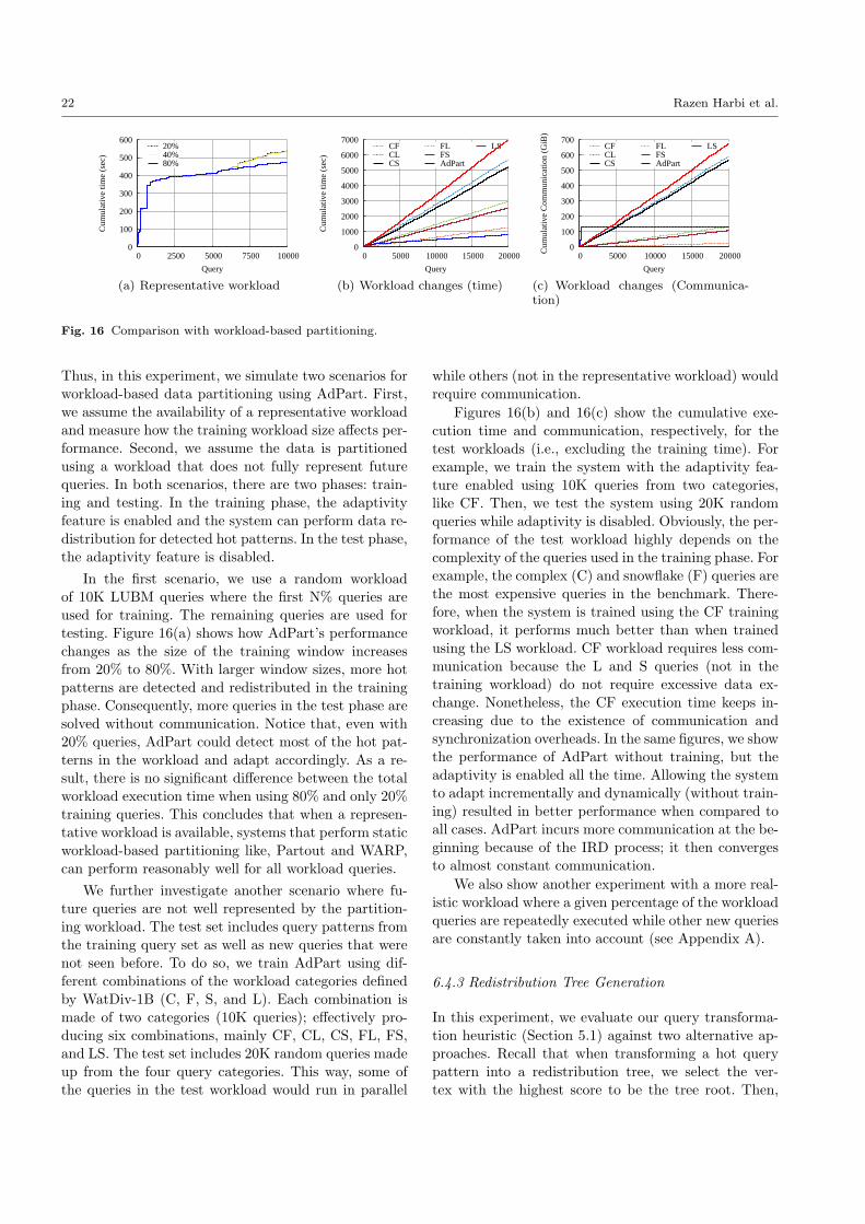
22 Razen Harbi et al.

0

100

200

300

400

500

600

0 2500 5000 7500 10000

Cum

ulat

ive

time

(sec

)

Query

20%40%80%

(a) Representative workload

0

1000

2000

3000

4000

5000

6000

7000

0 5000 10000 15000 20000

Cum

ulat

ive

time

(sec

)

Query

CFCLCS

FLFSAdPart

LS

(b) Workload changes (time)

0

100

200

300

400

500

600

700

0 5000 10000 15000 20000Cum

ulat

ive

Com

mun

icat

ion

(GiB

)

Query

CFCLCS

FLFSAdPart

LS

(c) Workload changes (Communica-tion)

Fig. 16 Comparison with workload-based partitioning.

Thus, in this experiment, we simulate two scenarios for

workload-based data partitioning using AdPart. First,

we assume the availability of a representative workloadand measure how the training workload size affects per-

formance. Second, we assume the data is partitioned

using a workload that does not fully represent futurequeries. In both scenarios, there are two phases: train-

ing and testing. In the training phase, the adaptivity

feature is enabled and the system can perform data re-distribution for detected hot patterns. In the test phase,

the adaptivity feature is disabled.

In the first scenario, we use a random workload

of 10K LUBM queries where the first N% queries areused for training. The remaining queries are used for

testing. Figure 16(a) shows how AdPart’s performance

changes as the size of the training window increasesfrom 20% to 80%. With larger window sizes, more hot

patterns are detected and redistributed in the training

phase. Consequently, more queries in the test phase are

solved without communication. Notice that, even with20% queries, AdPart could detect most of the hot pat-

terns in the workload and adapt accordingly. As a re-

sult, there is no significant difference between the totalworkload execution time when using 80% and only 20%

training queries. This concludes that when a represen-

tative workload is available, systems that perform staticworkload-based partitioning like, Partout and WARP,

can perform reasonably well for all workload queries.

We further investigate another scenario where fu-

ture queries are not well represented by the partition-ing workload. The test set includes query patterns from

the training query set as well as new queries that were

not seen before. To do so, we train AdPart using dif-ferent combinations of the workload categories defined

by WatDiv-1B (C, F, S, and L). Each combination is

made of two categories (10K queries); effectively pro-

ducing six combinations, mainly CF, CL, CS, FL, FS,and LS. The test set includes 20K random queries made

up from the four query categories. This way, some of

the queries in the test workload would run in parallel

while others (not in the representative workload) would

require communication.

Figures 16(b) and 16(c) show the cumulative exe-cution time and communication, respectively, for the

test workloads (i.e., excluding the training time). For

example, we train the system with the adaptivity fea-

ture enabled using 10K queries from two categories,like CF. Then, we test the system using 20K random

queries while adaptivity is disabled. Obviously, the per-

formance of the test workload highly depends on thecomplexity of the queries used in the training phase. For

example, the complex (C) and snowflake (F) queries are

the most expensive queries in the benchmark. There-fore, when the system is trained using the CF training

workload, it performs much better than when trained

using the LS workload. CF workload requires less com-

munication because the L and S queries (not in thetraining workload) do not require excessive data ex-

change. Nonetheless, the CF execution time keeps in-

creasing due to the existence of communication andsynchronization overheads. In the same figures, we show

the performance of AdPart without training, but the

adaptivity is enabled all the time. Allowing the systemto adapt incrementally and dynamically (without train-

ing) resulted in better performance when compared to

all cases. AdPart incurs more communication at the be-

ginning because of the IRD process; it then convergesto almost constant communication.

We also show another experiment with a more real-

istic workload where a given percentage of the workload

queries are repeatedly executed while other new queriesare constantly taken into account (see Appendix A).

6.4.3 Redistribution Tree Generation

In this experiment, we evaluate our query transforma-

tion heuristic (Section 5.1) against two alternative ap-proaches. Recall that when transforming a hot query

pattern into a redistribution tree, we select the ver-

tex with the highest score to be the tree root. Then,

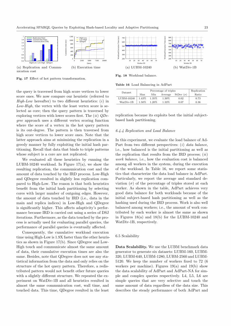
Accelerating SPARQL Queries by Exploiting Hash-based Locality and Adaptive Partitioning 23

0.4

0.6

0.8

1

1.2

1.4

1.6

1.8

2

High-Low Low-High QDegree

Replication RatioTouched Data RatioCommunication (TiB)

(a) Replication and Commu-nication cost

0

200

400

600

800

1000

1200

0 2500 5000 7500 10000

Cum

ulat

ive

time

(sec

)Query

High-LowLow-HighQDegree

(b) Execution time

Fig. 17 Effect of hot pattern transformation.

the query is traversed from high score vertices to lower

score ones. We now compare our heuristic (referred toHigh-Low hereafter) to two different heuristics: (i) in

Low-High, the vertex with the least vertex score is se-

lected as core; then the query pattern is traversed by

exploring vertices with lower scores first. The (ii) QDe-gree approach uses a different vertex scoring function

where the score of a vertex in the hot query pattern

is its out-degree. The pattern is then traversed fromhigh score vertices to lower score ones. Note that the

latter approach aims at minimizing the replication in a

greedy manner by fully exploiting the initial hash par-titioning. Recall that data that binds to triple patterns

whose subject is a core are not replicated.

We evaluated all these heuristics by running the

LUBM-10240 workload. In Figure 17(a), we show the

resulting replication, the communication cost and theamount of data touched by the IRD process. Low-High

and QDegree resulted in slightly less replication com-

pared to High-Low. The reason is that both heuristicsbenefit from the initial hash partitioning by selecting

cores with larger number of outgoing edges. However,

the amount of data touched by IRD (i.e., data in the

main and replica indices) in Low-High and QDegreeis significantly higher. This affects adaptivity’s perfor-

mance because IRD is carried out using a series of DSJ

iterations. Furthermore, as the data touched by the pro-cess is actually used for evaluating parallel queries, the

performance of parallel queries is eventually affected.

Consequently, the cumulative workload execution

time using High-Low is 1.9X faster than the other heuris-

tics as shown in Figure 17(b). Since QDegree and Low-High touch and communicate almost the same amount

of data, their cumulative execution times are also the

same. Besides, note that QDegree does not use any sta-tistical information from the data and only relies on the

structure of the hot query pattern. Therefore, a redis-

tributed pattern would not benefit other future queries

with a slightly different structure. We repeated the ex-periment on WatDiv-1B and all heuristics resulted in

almost the same communication cost, wall time, and

touched data. This time, QDegree resulted in the least

200

300

400

500

600

700

10 20 30 40 50 60 70

Wor

kloa

d E

xecu

tion

Tim

e (s

ec)

Worker ID

(a) LUBM-10240

200

300

400

500

600

700

800

900

10 20 30 40 50 60 70

Wor

kloa

d E

xecu

tion

Tim

e (s

ec)

Worker ID

(b) WatDiv-1B

Fig. 18 Workload balance.

Table 16 Load Balancing in AdPart

DatasetPercentage of triples Replication

RatioMax Min Average StDev (σ)

LUBM-10240 1.43% 1.35% 1.39% 0.02 0.73

WatDiv-1B 1.58% 1.20% 1.33% 0.07 0.36

replication because its exploits best the initial subject-based hash partitioning.

6.4.4 Replication and Load Balance

In this experiment, we evaluate the load balance of Ad-

Part from two different perspectives: (i) data balance,

i.e., how balanced is the initial partitioning as well asthe replication that results from the IRD process; (ii)

work balance, i.e., how the evaluation cost is balanced

among all workers in the system, during the execution

of the workload. In Table 16, we report some statis-tics that characterize the data load balance in AdPart.

Particularly, we report the average and standard de-

viation (σ) of the percentage of triples stored at eachworker. As shown in the table, AdPart achieves very

good data balance for both workloads because of the

initial subject-based hash partitioning as well as thehashing used during the IRD process. Work is also well

balanced among workers; i.e., the amount of work con-

tributed by each worker is almost the same as shown

in Figures 18(a) and 18(b) for the LUBM-10240 andWatDiv-1B, respectively.

6.5 Scalability

Data Scalability. We use the LUBM benchmark data

generator to generate six datasets: LUBM-160, LUBM-

320, LUBM-640, LUBM-1280, LUBM-2560 and LUBM-5120. We keep the number of workers fixed to 72 (6

workers per machine). Figures 19(a) and 19(b) show

the data scalability of AdPart and AdPart-NA for sim-

ple and complex queries respectively. L4, L5, L6 aresimple queries that are very selective and touch the

same amount of data regardless of the data size. This

describes the steady performance of both AdPart and

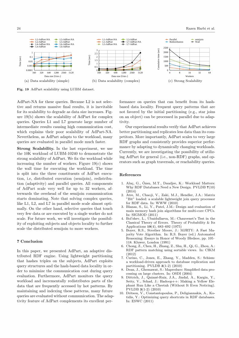
24 Razen Harbi et al.

0.0001

0.001

0.01

0.1

1

160 320 640 1280 2560 5120

Tim

e (s

ec)

Data size [Univ.]

L2-AdPart-NAL2-AdPartL4-AdPart-NAL4-AdPart

L5-AdPart-NAL5-AdPartL6-AdPart-NAL6-AdPart

(a) Data scalability (simple)

0

0.5

1

1.5

2

2.5

3

160 320 640 1280 2560 5120

Tim

e (s

ec)

Data size [Univ.]

L1-AdPart-NAL1-AdPartL3-AdPart-NA

L3-AdPartL7-AdPart-NAL7-AdPart

(b) Data scalability (complex)

0

500

1000

1500

2000

2500

4 8 16 32 64

Cum

ulat

ive

time

(sec

)

Workers

ParallelRedistribution

semijoinWall

(c) Strong Scalability

Fig. 19 AdPart scalability using LUBM dataset.

AdPart-NA for these queries. Because L2 is not selec-tive and returns massive final results, it is inevitable

for its scalability to degrade as data size increases. Fig-

ure 19(b) shows the scalability of AdPart for complexqueries. Queries L1 and L7 generate large number of

intermediate results causing high communication cost,

which explains their poor scalability of AdPart-NA.

Nevertheless, as AdPart adapts to the workload, manyqueries are evaluated in parallel mode much faster.

Strong Scalability. In the last experiment, we usethe 10K workload of LUBM-10240 to demonstrate the

strong scalability of AdPart. We fix the workload while

increasing the number of workers. Figure 19(c) showsthe wall time for executing the workload. The time

is split into the three constituents of AdPart execu-

tion, i.e, distributed execution (semijoin), redistribu-tion (adaptivity) and parallel queries. All components

of AdPart scale very well for up to 32 workers, af-

terwards the overhead of the semijoin communication

starts dominating. Note that solving complex queries,like L1, L2, and L7 in parallel mode scale almost opti-

mally. On the other hand, selective queries that touch

very few data or are executed by a single worker do notscale. For future work, we will investigate the possibil-

ity of exploiting subjects and objects locality to further

scale the distributed semijoin to more workers.

7 Conclusion

In this paper, we presented AdPart, an adaptive dis-tributed RDF engine. Using lightweight partitioning

that hashes triples on the subjects, AdPart exploits

query structures and the hash-based data locality in or-der to minimize the communication cost during query

evaluation. Furthermore, AdPart monitors the query

workload and incrementally redistributes parts of the

data that are frequently accessed by hot patterns. Bymaintaining and indexing these patterns, many future

queries are evaluated without communication. The adap-

tivity feature of AdPart complements its excellent per-

formance on queries that can benefit from its hash-based data locality. Frequent query patterns that are

not favored by the initial partitioning (e.g., star joins

on an object) can be processed in parallel due to adap-tivity.

Our experimental results verify that AdPart achieves

better partitioning and replicates less data than its com-

petitors. More importantly, AdPart scales to very largeRDF graphs and consistently provides superior perfor-

mance by adapting to dynamically changing workloads.

Currently, we are investigating the possibility of utiliz-ing AdPart for general (i.e., non-RDF) graphs, and op-

erators such as graph traversals, or reachability queries.

References

1. Aluc, G., Ozsu, M.T., Daudjee, K.: Workload Matters:Why RDF Databases Need a New Design. PVLDB 7(10)(2014)

2. Atre, M., Chaoji, V., Zaki, M.J., Hendler, J.A.: Matrix”Bit” loaded: a scalable lightweight join query processorfor RDF data. In: WWW (2010)

3. Blanas, S., Li, Y., Patel, J.M.: Design and evaluation ofmain memory hash join algorithms for multi-core CPUs.In: SIGMOD (2011)

4. Bol’shev, L., Ubaidullaeva, M.: Chauvenet’s Test in theClassical Theory of Errors. Theory of Probability & ItsApplications 19(4), 683–692 (1975)

5. Boyer, R.S., Strother Moore, J.: MJRTY: A Fast Ma-jority Vote Algorithm. In: R.S. Boyer (ed.) AutomatedReasoning: Essays in Honor of Woody Bledsoe, pp. 105–118. Kluwer, London (1991)

6. Chong, Z., Chen, H., Zhang, Z., Shu, H., Qi, G., Zhou, A.:RDF pattern matching using sortable views. In: CIKM(2012)

7. Curino, C., Jones, E., Zhang, Y., Madden, S.: Schism:a workload-driven approach to database replication andpartitioning. PVLDB 3(1-2) (2010)

8. Dean, J., Ghemawat, S.: Mapreduce: Simplified data pro-cessing on large clusters. In: OSDI (2004)

9. Dittrich, J., Quiane-Ruiz, J.A., Jindal, A., Kargin, Y.,Setty, V., Schad, J.: Hadoop++: Making a Yellow Ele-phant Run Like a Cheetah (Without It Even Noticing).PVLDB 3(1-2) (2010)

10. Dritsou, V., Constantopoulos, P., Deligiannakis, A., Ko-tidis, Y.: Optimizing query shortcuts in RDF databases.In: ESWC (2011)

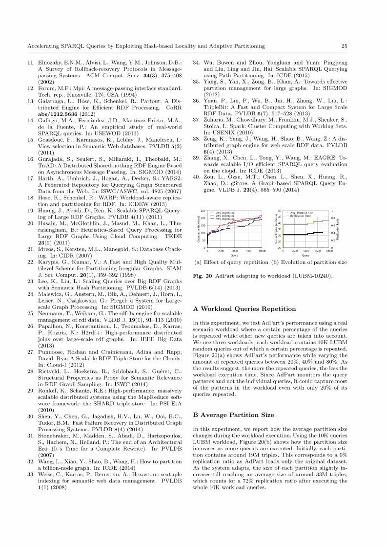
Accelerating SPARQL Queries by Exploiting Hash-based Locality and Adaptive Partitioning 25

11. Elnozahy, E.N.M., Alvisi, L., Wang, Y.M., Johnson, D.B.:A Survey of Rollback-recovery Protocols in Message-passing Systems. ACM Comput. Surv. 34(3), 375–408(2002)

12. Forum, M.P.: Mpi: A message-passing interface standard.Tech. rep., Knoxville, TN, USA (1994)

13. Galarraga, L., Hose, K., Schenkel, R.: Partout: A Dis-tributed Engine for Efficient RDF Processing. CoRRabs/1212.5636 (2012)

14. Gallego, M.A., Fernandez, J.D., Martınez-Prieto, M.A.,de la Fuente, P.: An empirical study of real-worldSPARQL queries. In: USEWOD (2011)

15. Goasdoue, F., Karanasos, K., Leblay, J., Manolescu, I.:View selection in Semantic Web databases. PVLDB 5(2)(2011)

16. Gurajada, S., Seufert, S., Miliaraki, I., Theobald, M.:TriAD: A Distributed Shared-nothing RDF Engine Basedon Asynchronous Message Passing. In: SIGMOD (2014)

17. Harth, A., Umbrich, J., Hogan, A., Decker, S.: YARS2:A Federated Repository for Querying Graph StructuredData from the Web. In: ISWC/ASWC, vol. 4825 (2007)

18. Hose, K., Schenkel, R.: WARP: Workload-aware replica-tion and partitioning for RDF. In: ICDEW (2013)

19. Huang, J., Abadi, D., Ren, K.: Scalable SPARQL Query-ing of Large RDF Graphs. PVLDB 4(11) (2011)

20. Husain, M., McGlothlin, J., Masud, M., Khan, L., Thu-raisingham, B.: Heuristics-Based Query Processing forLarge RDF Graphs Using Cloud Computing. TKDE23(9) (2011)

21. Idreos, S., Kersten, M.L., Manegold, S.: Database Crack-ing. In: CIDR (2007)

22. Karypis, G., Kumar, V.: A Fast and High Quality Mul-tilevel Scheme for Partitioning Irregular Graphs. SIAMJ. Sci. Comput. 20(1), 359–392 (1998)

23. Lee, K., Liu, L.: Scaling Queries over Big RDF Graphswith Semantic Hash Partitioning. PVLDB 6(14) (2013)

24. Malewicz, G., Austern, M., Bik, A., Dehnert, J., Horn, I.,Leiser, N., Czajkowski, G.: Pregel: a System for Large-scale Graph Processing. In: SIGMOD (2010)

25. Neumann, T., Weikum, G.: The rdf-3x engine for scalablemanagement of rdf data. VLDB J. 19(1), 91–113 (2010)

26. Papailiou, N., Konstantinou, I., Tsoumakos, D., Karras,P., Koziris, N.: H2rdf+: High-performance distributedjoins over large-scale rdf graphs. In: IEEE Big Data(2013)

27. Punnoose, Roshan and Crainiceanu, Adina and Rapp,David: Rya: A Scalable RDF Triple Store for the Clouds.In: Cloud-I (2012)

28. Rietveld, L., Hoekstra, R., Schlobach, S., Gueret, C.:Structural Properties as Proxy for Semantic Relevancein RDF Graph Sampling. In: ISWC (2014)

29. Rohloff, K., Schantz, R.E.: High-performance, massivelyscalable distributed systems using the MapReduce soft-ware framework: the SHARD triple-store. In: PSI EtA(2010)

30. Shen, Y., Chen, G., Jagadish, H.V., Lu, W., Ooi, B.C.,Tudor, B.M.: Fast Failure Recovery in Distributed GraphProcessing Systems. PVLDB 8(4) (2014)

31. Stonebraker, M., Madden, S., Abadi, D., Harizopoulos,S., Hachem, N., Helland, P.: The end of an ArchitecturalEra: (It’s Time for a Complete Rewrite). In: PVLDB(2007)

32. Wang, L., Xiao, Y., Shao, B., Wang, H.: How to partitiona billion-node graph. In: ICDE (2014)

33. Weiss, C., Karras, P., Bernstein, A.: Hexastore: sextupleindexing for semantic web data management. PVLDB1(1) (2008)

34. Wu, Buwen and Zhou, Yongluan and Yuan, Pingpengand Liu, Ling and Jin, Hai: Scalable SPARQL Queryingusing Path Partitioning. In: ICDE (2015)

35. Yang, S., Yan, X., Zong, B., Khan, A.: Towards effectivepartition management for large graphs. In: SIGMOD(2012)

36. Yuan, P., Liu, P., Wu, B., Jin, H., Zhang, W., Liu, L.:TripleBit: A Fast and Compact System for Large ScaleRDF Data. PVLDB 6(7), 517–528 (2013)

37. Zaharia, M., Chowdhury, M., Franklin, M.J., Shenker, S.,Stoica, I.: Spark: Cluster Computing with Working Sets.In: USENIX (2010)

38. Zeng, K., Yang, J., Wang, H., Shao, B., Wang, Z.: A dis-tributed graph engine for web scale RDF data. PVLDB6(4) (2013)

39. Zhang, X., Chen, L., Tong, Y., Wang, M.: EAGRE: To-wards scalable I/O efficient SPARQL query evaluationon the cloud. In: ICDE (2013)

40. Zou, L., Ozsu, M.T., Chen, L., Shen, X., Huang, R.,Zhao, D.: gStore: A Graph-based SPARQL Query En-gine. VLDB J. 23(4), 565–590 (2014)

0

50

100

150

200

250

0 2500 5000 7500 10000

Cum

ulat

ive

time

(sec

)

Query

20% Repetition40% Repetition80% Repetition

(a) Effect of query repetition

20

25

30

35

40

45

50

0 2500 5000 7500 10000 0

0.2

0.4

0.6

0.8

1

Size

in T

ripl

es (

mill

ions

)

Rep

licat

ion

Rat

io

Query

Avg. Partition SizeReplication Ratio

(b) Evolution of partition size

Fig. 20 AdPart adapting to workload (LUBM-10240).

A Workload Queries Repetition

In this experiment, we test AdPart’s performance using a realscenario workload where a certain percentage of the queriesis repeated while other new queries are taken into account.We use three workloads, each workload contains 10K LUBMrandom queries out of which a certain percentage is repeated.Figure 20(a) shows AdPart’s performance while varying theamount of repeated queries between 20%, 40% and 80%. Asthe results suggest, the more the repeated queries, the less theworkload execution time. Since AdPart monitors the querypatterns and not the individual queries, it could capture mostof the patterns in the workload even with only 20% of itsqueries repeated.

B Average Partition Size

In this experiment, we report how the average partition sizechanges during the workload execution. Using the 10K queriesLUBM workload, Figure 20(b) shows how the partition sizeincreases as more queries are executed. Initially, each parti-tion contains around 19M triples. This corresponds to a 0%replication ratio as AdPart loads only the original dataset.As the system adapts, the size of each partition slightly in-creases till reaching an average size of around 33M triples;which counts for a 72% replication ratio after executing thewhole 10K workload queries.

26 Razen Harbi et al.

C LUBM Benchmark Queries

PREFIX rdf: <http://www.w3.org/1999/02/22-rdf-syntax-ns#>

PREFIX ub: <http://www.lehigh.edu/ zhp2/2004/0401/univ-bench.owl#>

PREFIX rdfs: <http://www.w3.org/2000/01/rdf-schema#>

Q1: SELECT ?X WHERE{

?X rdf:type ub:GraduateStudent .?X ub:takesCourse <http://www.Department0.University0.edu/GraduateCourse0> .}Q2: SELECT ?X ?Y ?Z WHERE{?X rdf:type ub:GraduateStudent .?Y rdf:type ub:University .?Z rdf:type ub:Department .?X ub:memberOf ?Z .?Z ub:subOrganizationOf ?Y .?X ub:undergraduateDegreeFrom ?Y .}Q3: SELECT ?X WHERE{?X rdf:type ub:Publication .?X ub:publicationAuthor <http://www.Department0.University0.edu/AssistantProfessor0> .}Q4: SELECT ?X, ?Y1, ?Y2, ?Y3 WHERE?X rdf:type ub:AssociateProfessor .?X ub:worksFor <http://www.Department0.University0.edu> .?X ub:name ?Y1 .?X ub:emailAddress ?Y2 .?X ub:telephone ?Y3 .}Q5: SELECT ?X WHERE{?X rdf:type ub:UndergraduateStudent .?X ub:memberOf <http://www.Department0.University0.edu> .}Q6: SELECT ?X WHERE{?X rdf:type ub:UndergraduateStudent .}Q7: SELECT ?X, ?Y WHERE{?X rdf:type ub:UndergraduateStudent .?Y rdf:type ub:Course .?X ub:takesCourse ?Y .<http://www.Department0.University0.edu/AssociateProfessor0> ub:teacherOf ?Y .}Q8: SELECT ?X, ?Y, ?Z WHERE{?X rdf:type ub:UndergraduateStudent .?Y rdf:type ub:Department .?X ub:memberOf ?Y .?Y ub:subOrganizationOf <http://www.University0.edu> .?X ub:emailAddress ?Z .}Q9: SELECT ?X, ?Y, ?Z WHERE{?X rdf:type ub:GraduateStudent .?Y rdf:type ub:AssociateProfessor .?Z rdf:type ub:GraduateCourse .?X ub:advisor ?Y .?Y ub:teacherOf ?Z .?X ub:takesCourse ?Z .}Q10: SELECT ?X WHERE{?X rdf:type ub:TeachingAssistant .?X ub:takesCourse <http://www.Department0.University0.

edu/GraduateCourse0> .}Q11: SELECT ?X WHERE{

?X rdf:type ub:ResearchGroup .?X ub:subOrganizationOf ?Z .?Z ub:subOrganizationOf <http://www.University0.edu> .}Q12: SELECT ?X, ?Y WHERE{?Y rdf:type ub:Department .?X ub:headOf ?Y.?Y ub:subOrganizationOf <http://www.University0.edu> .}Q13: SELECT ?X WHERE{?X rdf:type ub:GraduateStudent .?X ub:undergraduateDegreeFrom <http://www.University0.edu> .}Q14: SELECT ?X WHERE{

?X rdf:type ub:GraduateStudent .}

D LUBM Workload

We generated a workload of 20,000 queries from LUBM bench-mark queries shown in C. For queries that do not have con-stants (Q2 and Q9), we generate different query patterns byremoving some triples and mutating the node types. For ex-ample, in Q2, we generated 18 different patterns by alternat-ing student type between UndergraduateStudent and Grad-uateStudent (see Table 17). Similarly, other query patternsare generated by removing different combinations of the querytriple patterns. We did not generate variations of Q6 and Q14as they have only one triple pattern (rdf:type) with a singleconstant. For the rest of the queries, we generated 1000 dif-ferent patterns from each query by varying the values of thequery constants. For example, in Q1, we generate differentquery patterns by varying the values of both student type(UndergraduateStudent or GraduateStudent) and graduatecourses.

Table 17 LUBM Workload

Patterns Changes

Q1 1000 Constants

Q2 18 Structure/Constants

Q3 1000 Constants

Q4 1000 Constants

Q5 1000 Constants

Q6 1 No Changes

Q7 1000 Constants

Q8 1000 Constants

Q9 30 Structure/Constants

Q10 1000 Constants

Q11 1000 Constants

Q12 1000 Constants

Q13 1000 Constants

Q14 1 No Changes

Accelerating SPARQL Queries by Exploiting Hash-based Locality and Adaptive Partitioning 27

E YAGO2 Queries

PREFIX y: <http://yago-knowledge.org/resource/>Y1: SELECT ?GivenName ?FamilyName WHERE{?p y:hasGivenName ?GivenName .?p y:hasFamilyName ?FamilyName .?p y:wasBornIn ?city .?p y:hasAcademicAdvisor ?a .?a y:wasBornIn ?city .}

Y2: SELECT ?GivenName ?FamilyName WHERE{?p y:hasGivenName ?GivenName .?p y:hasFamilyName ?FamilyName .?p y:wasBornIn ?city .?p y:hasAcademicAdvisor ?a .?a y:wasBornIn ?city .?p y:isMarriedTo ?p2 .?p2 y:wasBornIn ?city .}

Y3: SELECT ?name1 ?name2 WHERE{

?a1 y:hasPreferredName ?name1 .?a2 y:hasPreferredName ?name2 .?a1 y:actedIn ?movie .?a2 y:actedIn ?movie .}

Y4: SELECT ?name1 ?name2 WHERE{?p1 y:hasPreferredName ?name1 .?p2 y:hasPreferredName ?name2 .?p1 y:isMarriedTo ?p2 .?p1 y:wasBornIn ?city .?p2 y:wasBornIn ?city .}

F Bio2RDF

PREFIX pharmkb: <http://bio2rdf.org/pharmgkb vocabulary>PREFIX irefindex: <http://bio2rdf.org/irefindex vocabulary>PREFIX pubmd: <http://bio2rdf.org/pubmed vocabulary>PREFIX pubmdrc: <http://bio2rdf.org/pubmed resource>PREFIX omim:<http://bio2rdf.org/omim vocabulary>PREFIX drug:<http://bio2rdf.org/drugbank>PREFIX uniprot:<http://bio2rdf.org/uniprot>B1: SELECT ?o WHERE{pubmdrc:1374967 INVESTIGATOR 1 pubmd:last name ?o .pubmdrc:1374967 AUTHOR 1 pubmd:last name ?o .}B2: SELECT ?articleToMesh WHERE{

<http://bio2rdf.org/pubmed:126183> pubmd:mesh heading?articleToMesh .?articleToMesh pubmd:mesh descriptor name ?mesh .}

B3: SELECT ?phenotype WHERE{?phenotype rdf:type omim:Phenotype .?phenotype rdfs:label ?label .?gene omim:phenotype ?phenotype .}

B4: SELECT ?pharmgkbid WHERE{?pharmgkbid pharmkb:xref drug:DB00126 .?pharmgkbid pharmkb:xref ?pccid .?DDIassociation pharmkb:chemical ?pccid .?DDIassociation pharmkb:event ?DDIevent .?DDIassociation pharmkb:chemical ?drug2 .

?DDIassociation pharmkb:p-value ?pvalue .}

B5: SELECT ?interaction WHERE{

?interaction irefindex:interactor a uniprot:O17680 .}