Embed Size (px)
Citation preview

RESEARCH ARTICLE
Accelerating cross-validation with total
variation and its application to super-
resolution imaging
Tomoyuki Obuchi1*, Shiro Ikeda2, Kazunori Akiyama3,4,5, Yoshiyuki Kabashima1
1 Department of Mathematical and Computing Science/Tokyo Institute of Technology, Yokohama 226-8502,
Japan, 2 The Institute of Statistical Mathematics, Tachikawa, Tokyo, 190-8562, Japan, 3 Haystack
Observatory/Massachusetts Institute of Technology, Westford, MA, 01886, United States of America,
4 National Astronomy Observatory of Japan, Osawa 2-21-1, Mitaka, Tokyo 181-8588, Japan, 5 Black Hole
Initiative, Harvard University, Cambridge, MA, 02138, United States of America
Abstract
We develop an approximation formula for the cross-validation error (CVE) of a sparse linear
regression penalized by ℓ1-norm and total variation terms, which is based on a perturbative
expansion utilizing the largeness of both the data dimensionality and the model. The devel-
oped formula allows us to reduce the necessary computational cost of the CVE evaluation
significantly. The practicality of the formula is tested through application to simulated black-
hole image reconstruction on the event-horizon scale with super resolution. The results
demonstrate that our approximation reproduces the CVE values obtained via literally con-
ducted cross-validation with reasonably good precision.
1 Introduction
At present, in many practical situations of science and technology, large high-dimensional
observational datasets are created and accumulated on a continuous basis. An essential diffi-
culty concerning the treatment of such high-dimensional data is the extraction of meaningful
information. Sparse modeling [1, 2] is a promising framework for overcoming this difficulty,
which has recently been utilized in many disciplines [3, 4]. In this framework, a statistical or
machine-learning model with a large number of parameters (explanatory variables) is fitted to
the data, in conjunction with a certain sparsity-inducing penalty. This penalty should be
appropriately chosen with consideration of the processed data. One representative penalty is
the ℓ1 regularization, which retains certain preferred properties, such as the statistical model
convexity [5, 6]. A similar penalty that has received more recent focus is the so-called “total
variation (TV)” [7–9], which can be regarded as the ℓ1 regularization imposed on the differ-
ence between neighboring explanatory variables. The TV yields “continuity” of the neighbor-
ing variables, which is suitable for the processing of certain datasets expected to have such
continuity, such as natural images [4, 7–9].
Another common difficulty associated with the use of statistical models is model selection.
In the context of image processing using the ℓ1 and TV regularizations, this difficulty appears
PLOS ONE | https://doi.org/10.1371/journal.pone.0188012 December 7, 2017 1 / 14
a1111111111
a1111111111
a1111111111
a1111111111
a1111111111
OPENACCESS
Citation: Obuchi T, Ikeda S, Akiyama K, Kabashima
Y (2017) Accelerating cross-validation with total
variation and its application to super-resolution
imaging. PLoS ONE 12(12): e0188012. https://doi.
org/10.1371/journal.pone.0188012
Editor: Yuanquan Wang, Beijing University of
Technology, CHINA
Received: December 10, 2016
Accepted: October 30, 2017
Published: December 7, 2017
Copyright: © 2017 Obuchi et al. This is an open
access article distributed under the terms of the
Creative Commons Attribution License, which
permits unrestricted use, distribution, and
reproduction in any medium, provided the original
author and source are credited.
Data Availability Statement: All image data used
in the paper are available from http://vlbiimaging.
csail.mit.edu/imagingchallenge.
Funding: This work was supported by Japan
Society for the Promotion of Science 25120008 to
Prof. Shiro Ikeda; 26870185 to Dr. Tomoyuki
Obuchi; 25120013 to Prof. Yoshiyuki Kabashima;
17H00764 to Dr. Tomoyuki Obuchi and Prof.
Yoshiyuki Kabashima; Research Abroad Program
to Dr. Kazunori Akiyama; and National Science
Foundation AST-1614868 to Dr. Kazunori Akiyama.

during the selection of appropriate regularization weights. A practical framework to select
these weights, which is applicable to general situations, is cross-validation (CV). CV provides
an estimator of the statistical-model generalization error, i.e., the CV error (CVE), using the
data under control, and the minimum CVE obtained when sweeping the weights yields the
optimal weight values. This versatile framework is, however, computationally demanding for
large datasets/models, and this problem frequently becomes a bottleneck affecting model selec-
tion. Thus, reducing the CVE computational cost could have a significant impact on a broad
range of sparse modeling applications in various disciplines.
Considering these circumstances, in this paper, we provide a CVE approximation formula
for a statistical model of linear regression penalized by the ℓ1 and TV terms, to efficiently
reduce the computational cost. Note that the formula for the case penalized by the ℓ1 term
alone has already been proposed in [10], and the formula presented herein is a generalization
of it. Below, we show the formula derivation and perform a demonstration in the context of
super-resolution imaging. The processed images employed in this study are reconstructed
from simulated observations of black holes on the event-horizon scale for the Event Horizon
Telescope (EHT, see [11–13]) full array. Note that our formula will be applied to actual EHT
observations to be conducted after April 2017.
2 Problem setting
Let us suppose that our measurement is a linear process, and denote the measurement result as
y 2 RM and the measurement matrix as A = {Aμi}μ=1,� � �,M; i=1,� � �N 2 RM×N. The explanatory var-
iables, corresponding to the images that will be examined in the later demonstration, are
denoted by x 2 RN. The quality of the fit to the data is described by the residual sum of squares
(RSS), i.e., Eðxjy;AÞ ¼ 1
2jjy � Axjj2
2. In addition, we consider the following penalty consisting
of ℓ1 and TV terms:
Rðx; l‘1; lTÞ ¼ l‘1
jjxjj1þ lTTðxÞ; ð1Þ
where the T(x) term corresponds to the TV and is expressed as
TðxÞ ¼P
i
ffiffiffiffiffiffiffiX
j2@i
s
ðxj � xiÞ2�X
i
ti; ð2Þ
and @i denotes the neighboring variables of the ith variable. There is some variation in the defi-
nition of “neighbors”; here, we follow the standard approach [7–9]. That is, x is assumed to be
a two-dimensional image and the neighbors of the ith pixel correspond to the right and down
pixels. However, the bottom row (the rightmost column) of the image is exceptional, as the
neighbor of each pixel in that row (column) corresponds to the right (down) pixel only. Note
that the developed approximation formula presented below is independent of this specific
choice of neighbors and can be applied to general cases.
For this setup, we consider the following linear regression problem with the penalty given
in Eq (1)
xðl‘1; lTÞ ¼ arg min
xfEðxjy;AÞ þ Rðx; l‘1
; lTÞg; ð3Þ
where arg minuff ðuÞg generally represents the argument that minimizes an arbitrary function
Accelerating cross-validation with total variation and its application to super-resolution imaging
PLOS ONE | https://doi.org/10.1371/journal.pone.0188012 December 7, 2017 2 / 14
Competing interests: The authors have declared
that no competing interests exist.

f(u). Further, we consider the leave-one-out (LOO) CV of Eq (3) in the form
xnmðl‘1; lTÞ ¼ argmin
x
1
2
X
nð6¼mÞ
ðyn � AnixiÞ2þ R
( )
� argminxfEðxjynm;AnmÞ þ Rðx; l‘1
; lTÞg: ð4Þ
Note that the system without the μth row of y and A is referred to as the “μth LOO system”
hereafter. In this procedure, the CVE, i.e., the generalization error estimator, is
ELOOðl‘1; lTÞ ¼
1
2
XM
m¼1
ðym � aTmxnmðl‘1
; lTÞÞ2; ð5Þ
where a>m¼ ðAm1; � � � ;AmNÞ is the μth row vector of A. We term this simply the “LOO error
(LOOE).”
Computing the LOOE requires solution of Eq (4) M times, by definition, which is computa-
tionally expensive. Therefore, the purpose of this paper is to avoid this computational expense
by deriving an approximation formula of Eq (5).
3 Approximation formula for softened system
When M is sufficiently large, i.e., the number of observations is large enourgh, the difference
between the LOO solution xnm and the full solution x is expected to be small. This intuition
naturally motivates us to conduct a perturbation connecting these two solutions. To conduct
this perturbation, we “soften” the penalty by introducing a small cutoff δ(> 0) in the TV, hav-
ing the form
R! Rdðx; l‘1; lTÞ ¼ l‘1
X
i
jjxjj þ lTTdðxÞ; ð6Þ
where
Td ¼X
i
ffiffiffiffiffiffiffiffiffiffiffiffiffiffiffiffiffiffiffiffiffiffiffiffiffiffiffiffiffiffiffiffiffiffiffiX
j2@i
ðxj � xiÞ2þ d
2
s
�X
i
td
i : ð7Þ
An approximation formula in the presence of ℓ1 regularization with smooth cost functions has
already been proposed in [10]. We employ that formula here and take the limit δ! 0.
To state the approximation formula, we begin by defining “active” and “killed” variables.
Owing to the ℓ1 term, some variables are set to zero in x; we refer to these variables as “killed
variables.” The remaining finite variables are termed “active variables.” We denote the index
sets of the active and killed variables by SA and SK, respectively. The active (killed) components
of a vector x are formally expressed as xSA(xSK). For any matrix X, we use double subscripts in
the same manner. For example, for an N × N matrix, a submatrix having row and column
components of SA and SK, respectively, is denoted by XSA SK.
The approximation formula can be derived through the following two steps. Note that, in
this derivation, a crucial assumption is that the sets of active and killed variables are common
among the full and LOO systems. This assumption may not hold exactly in practice, but the
resultant formula is asymptotically exact in the large-N limit [10].
The first step is to compute the values of the active variables and their response to small per-
turbation. The active variables are determined by the extremization condition of the softened
Accelerating cross-validation with total variation and its application to super-resolution imaging
PLOS ONE | https://doi.org/10.1371/journal.pone.0188012 December 7, 2017 3 / 14

cost function with respect to the active variables, such that
@ðEðxjynm;AnmÞ þ Rdðx; l‘1; lTÞÞ
@xSA¼ 0) ðxdnmÞSA : ð8Þ
The focus here is the response of this solution when a small perturbation −h � x is incorporated
into the cost function. A simple computation demonstrates that the active–active components
of the response function, ðwdnmÞSASA ¼@
@hSAðxdnmÞSA jh¼0, are equivalent to the inverse of the cost-
function Hessian
ðwdnmÞSASA ¼ ðHdnm
SASAÞ� 1; ð9Þ
Hdnm ¼ @2
xðEðxjynm;AnmÞ þ Rdðx; l‘1
; lTÞÞ ¼ Gnm þ @2
xRdðx; l‘1
; lTÞ; ð10Þ
where @2
x denotes the Hessian operator @2
x �@2
@xi@xj
� �and Gnμ is the Gram matrix of Anμ, i.e.,
Gnμ� (Anμ)> Anμ. The other components of the response function are identically zero, from
the stability assumption of SK and because the killed variables are zero, with xSK¼ xnmSK ¼ 0.
In the second step, we connect the full solution to the LOO solution, through the above per-
turbation with an appropriate h. To specify the perturbation, we assume that the difference
dd¼ xd � xdnm is small and expand the RSS of the full system with respect to dδ as follows:
Eðxdnmjy;AÞ�Eðxdjy;AÞ�XM
m¼1
ðym � a>
mxdÞa>
mdd: ð11Þ
This equation implies that the perturbation between the full and LOO systems can be
expressed as hm ¼ ðym � a>mxdÞam. Hence, we obtain
xd� xdnmþwdnmhm¼ xdnmþðym � a>m xdÞwdnmam: ð12Þ
The Hessian of the full system has a simple relationship with the LOO Hessian, such that
Hd � Gnm þ ðama>m Þ þ @2
xRdðxdÞ � Hdnm þ ðama>m Þ; ð13Þ
where the approximation at the righthand side comes from replacing xd with xdnm in the argu-
ment of Rδ(x). Inserting Eqs (12 and 13) in conjunction with wdSASA¼ ðHd
SASA� 1
into Eq (5) and
using the Sherman-Morrison formula for matrix inversion, we find
ELOOðl‘1; lTÞ�
1
2
XM
m¼1
ðym � a>mxdÞ
2
ð1� a>mSAðwdÞSASAamSA
Þ2: ð14Þ
According to Eq (14), we can compute the LOOE only from the full solution xd, without actu-
ally performing CV, which facilitates considerable reduction of the computational cost.
4 Handling a singularity
Let us generalize Eq (14) to the limit δ! 0, where the penalty contains another singular term
in addition to the ℓ1 term. This TV singularity tends to “lock” some of the neighboring vari-
ables, i.e., xj = xi (8j 2 @i), which corresponds to ti = 0 in Eq (2). If two different vanishing TV
terms, ti and tj, share a common variable xr, all the variables in those TV terms take the same
value xk = xr (8k 2 ({i} [ @i [ {j} [ @j)). In this manner, the active variables are separated into
several “locked” clusters, with all the variables inside a cluster having an identical value. This
Accelerating cross-validation with total variation and its application to super-resolution imaging
PLOS ONE | https://doi.org/10.1371/journal.pone.0188012 December 7, 2017 4 / 14

implies that the variable response to a perturbation, χ = limδ!0 χδ, should have the same value
for all variables in a cluster and may, therefore, be merged. Below, we demonstrate this behav-
ior for the δ! 0 limit. For the derivation, we assume that the clusters are common to both the
full and LOO systems, similar to the assumption for SA and SK. For convenience, we index the
clusters by α, β 2 C and denote the number of clusters by |C|; the index set of variables in a
cluster α is represented by Sα and the total set of indices in all clusters is denoted by SC� [αSα. Hereafter, we concentrate on the active variable space only and omit the killed variable
space. The complement set of SC, i.e., the set of isolated variables that do not belong to any clus-
ter, is denoted by SI and, thus, SA = SI [ SC.
Two crucial observations for the derivation are the “scale separation” and the presence of
the “zero mode.” For vanishing TV terms, a natural scaling to satisfy lim d!0tdi ¼ ti ¼ 0 is
jxdj � xd
i j / d ð8j 2 @iÞ. Once this scaling is assumed, we realize that the components of the
Hessian that are directly related to the clusters diverge. Let us define by Sa the set of TV terms
corresponding to cluster α, i.e., Sa ¼ fijðfig [ @iÞ � Sag. Hence, by construction and for all
α 2 C, all components of Dda� lTð@
2
x
Pi2Sa
tdi ÞSaSa
are scaled as 1/δ and, thus, diverge as δ! 0.
The remaining terms are retained as O(1). According to this “scale separation,” we decompose
the Hessian as Hδ = Dδ + Fδ, where Dδ is the direct sum of the diverging components in the
naively extended space; Dd ¼ �a Dda; and Fδ consists of the remaining O(1) terms. This decom-
position can be schematically expressed as
Hd ¼ Dd þ Fd ¼
Dd1
0 0
0 . ..
0
0 0 DdjCj
0
0 0
0
BBBB@
1
CCCCAþ
FdSCSC
FdSCSI
FdSI SC
FdSI SI
0
@
1
A: ð15Þ
We denote the basis of the current expression by {ei}i2SA, with (ei)j = δij, and move to
another basis that diagonalizes DdSCSC
. Each Dda
has a “zero mode,” and its normalized eigenvec-
tor is given by zα = (ziα), where zia ¼ 1=ffiffiffiffiffiffiffijSaj
pfor i 2 Sα and 0 otherwise, in the full space. This
behavior originates from the symmetry, such that the ftdi gi2Sa
are invariant under a uniform
shift in the Sα sub-space, i.e., xj! xj + Δ (8j 2 Sα) for 8Δ 2 R. This invariance can also be
directly seen from a property of the Hessian, i.e., @2
@x2itdi þ
Pj2@i
@
@xi@xjtdi ¼ 0.
In addition, we represent the set of normalized eigenvectors of all the other modes of Dda,
which have eigenvalues λαa that are proportional to 1/δ and positively divergent, as fuaagjSa j� 1
a¼1.
Then, {{{uαa}a, zα}α} diagonalizes DdSCSC
and {{{uαa}a, zα}α, {ei}i2SI} constitutes an orthonormal
basis of the full space. Corresponding to this variable change, we denote SZ , SIþZ , and SC� Z as
the index set of variables in the space spanned by {zα}α, {{zα}α, {ei}i2SI, and {uαa}α,a, respectively.
In the new expression, we can rewrite Hδ = Dδ + Fδ as
Hd ¼Dd
~SC� Z~SC� Z0
0 0
!
þFd
~SC� Z~SC� ZFd
~SC� Z~SIþZ
Fd~SIþZ~SC� Z
Fd~SIþZ~SIþZ
!
; ð16Þ
where Dd~SC� Z~SC� Z
¼ diagðflaaga;aÞ. Because of the divergence of Dd~SC� Z~SC� Z
, only Fd~SIþZ~SIþZ
is
Accelerating cross-validation with total variation and its application to super-resolution imaging
PLOS ONE | https://doi.org/10.1371/journal.pone.0188012 December 7, 2017 5 / 14

relevant for the evaluation of (Hδ)−1. These considerations yield the explicit formula of χ as
ðHdÞ� 1¼ðDd
~SC� Z~SC� Z� 1
0
0 ðFd~SIþZ ~SIþZ
Þ� 1
0
@
1
A þOðdÞ !0 0
0 ðF~SIþZ~SIþZÞ� 1
!
¼ w; ð17Þ
where F = limδ!0 Fδ.By construction, in the reduced space to span ({zα}α, {ei}i2SI), F~SIþZ~SIþZ
can be expressed as
F~SIþZ~SIþZ¼X
a;b
ðFabzaz>
bþ Fbazbz
>
aÞ þ
X
a
X
i2SI
ðFaizae>
i þ Fiaeiz>
aÞ þ
X
i;j2SI
Fijeie>
j : ð18Þ
As the non-zero components of the zero mode zα are identically given as 1=ffiffiffiffiffiffiffijSaj
p, all these
coefficients can be easily expressed by the original coefficients Fij, as
Fab ¼ z>aFzb ¼
1ffiffiffiffiffiffiffiffiffiffiffiffiffiffijSajjSbj
qX
i2Sa ;j2Sb
Fij; ð19aÞ
Fai ¼ z>aFei ¼
1ffiffiffiffiffiffiffijSaj
pX
j2Sa
Fji; ð19bÞ
and Fiα = Fαi by the symmetry. Now, all the components are explicitly specified. The form of χin the original basis {ei}i2SA can be accordingly assessed by moving back from the basis
{{{uαa}a, zα}α, {ei}i2SI}, which completes the computation.
Some additional consideration of the above computation demonstrates that we can shorten
some steps and obtain a more interpretable result. We introduce a j~SIþZj � j~SIþZjmatrix �F as
�F ab ¼ffiffiffiffiffiffiffiffiffiffiffiffiffiffijSajjSbj
qFab;
�F ai ¼ffiffiffiffiffiffiffijSaj
pFai; ð20Þ
with the remaining components being identical to those of F~SIþZ~SIþZ, i.e., �FSISI
¼ FSISI . Eqs (19)
and (20) indicate that �F is simply the matrix summing the rows and columns in each cluster to
a row and a column. It is natural that �F has a direct connection to χ, because the locked vari-
ables in a cluster should exhibit the same response against perturbation. In fact, the response
function χ in the original basis is expressed using �F as
w ¼X
i;j2SI
�F � 1
ij ðeie>
j þ eje>
i Þ þX
a;b
�F � 1
ab
X
i2Sa
X
j2Sb
eie>
j
þX
a
X
i2Sa
X
j2SI
�F � 1
aj eie>
j þX
i2SI
X
j2Sa
�F � 1
ia eie>
j
!
: ð21Þ
This can be directly shown from Eqs (17 and 19), using the relation F~SIþZ~SIþZ¼ P�F ~SIþZ ~SIþZ
P
with P ¼ diagðff1gi2SI ; fffiffiffiffiffiffiffijSaj
p � 1
gagÞ, and the blockwise matrix inversion formula. Eqs (14)
and (21) constitute the main result of this paper.
5 Algorithmic implementation
5.1 Numerical stability and the softening constant δFor handling the singularity of the cost-function Hessian, we have introduced the softening
constant δ in the TV and finally taken the δ! 0 limit. In practical implementations, however,
we should keep δ small but finite. To see the reason, it is sufficient to see a simple example with
Accelerating cross-validation with total variation and its application to super-resolution imaging
PLOS ONE | https://doi.org/10.1371/journal.pone.0188012 December 7, 2017 6 / 14
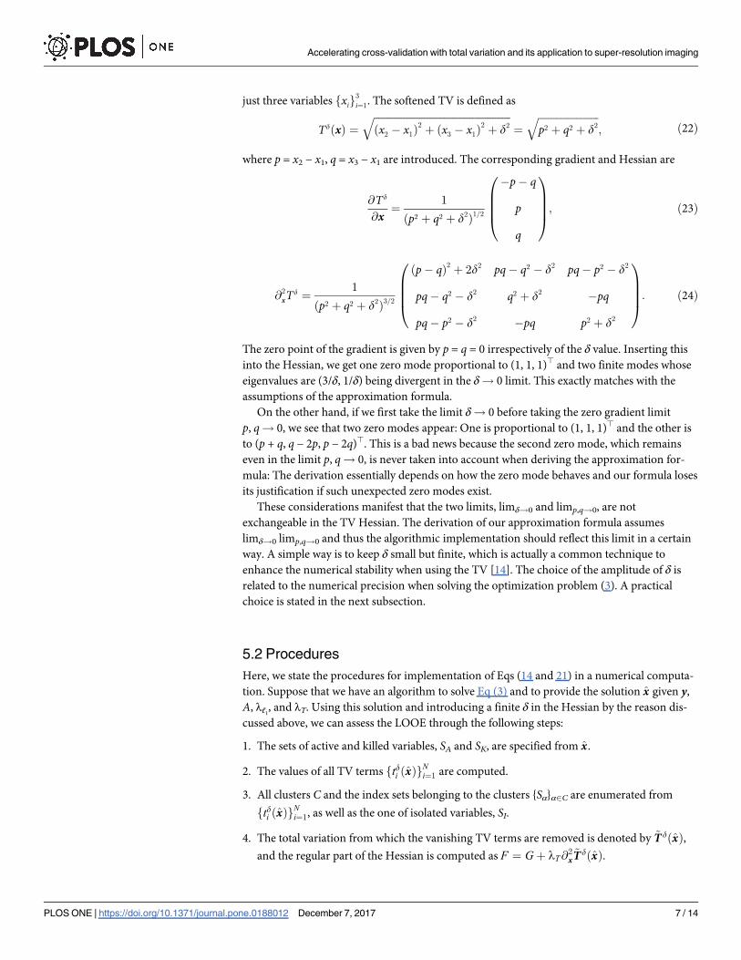
just three variables fxig3
i¼1. The softened TV is defined as
TdðxÞ ¼ffiffiffiffiffiffiffiffiffiffiffiffiffiffiffiffiffiffiffiffiffiffiffiffiffiffiffiffiffiffiffiffiffiffiffiffiffiffiffiffiffiffiffiffiffiffiffiffiffiffiffiffiffiffi
ðx2 � x1Þ2þ ðx3 � x1Þ
2þ d
2
q
¼
ffiffiffiffiffiffiffiffiffiffiffiffiffiffiffiffiffiffiffiffiffiffiffiffi
p2 þ q2 þ d2
q
; ð22Þ
where p = x2 − x1, q = x3 − x1 are introduced. The corresponding gradient and Hessian are
@Td
@x¼
1
ðp2 þ q2 þ d2Þ
1=2
� p � q
p
q
0
BBB@
1
CCCA; ð23Þ
@2
xTd ¼
1
ðp2 þ q2 þ d2Þ
3=2
ðp � qÞ2 þ 2d2 pq � q2 � d
2 pq � p2 � d2
pq � q2 � d2 q2 þ d
2� pq
pq � p2 � d2
� pq p2 þ d2
0
BBB@
1
CCCA: ð24Þ
The zero point of the gradient is given by p = q = 0 irrespectively of the δ value. Inserting this
into the Hessian, we get one zero mode proportional to (1, 1, 1)> and two finite modes whose
eigenvalues are (3/δ, 1/δ) being divergent in the δ! 0 limit. This exactly matches with the
assumptions of the approximation formula.
On the other hand, if we first take the limit δ! 0 before taking the zero gradient limit
p, q! 0, we see that two zero modes appear: One is proportional to (1, 1, 1)> and the other is
to (p + q, q − 2p, p − 2q)>. This is a bad news because the second zero mode, which remains
even in the limit p, q! 0, is never taken into account when deriving the approximation for-
mula: The derivation essentially depends on how the zero mode behaves and our formula loses
its justification if such unexpected zero modes exist.
These considerations manifest that the two limits, limδ!0 and limp,q!0, are not
exchangeable in the TV Hessian. The derivation of our approximation formula assumes
limδ!0 limp,q!0 and thus the algorithmic implementation should reflect this limit in a certain
way. A simple way is to keep δ small but finite, which is actually a common technique to
enhance the numerical stability when using the TV [14]. The choice of the amplitude of δ is
related to the numerical precision when solving the optimization problem (3). A practical
choice is stated in the next subsection.
5.2 Procedures
Here, we state the procedures for implementation of Eqs (14 and 21) in a numerical computa-
tion. Suppose that we have an algorithm to solve Eq (3) and to provide the solution x given y,
A, λℓ1, and λT. Using this solution and introducing a finite δ in the Hessian by the reason dis-
cussed above, we can assess the LOOE through the following steps:
1. The sets of active and killed variables, SA and SK, are specified from x.
2. The values of all TV terms ftdi ðxÞgNi¼1 are computed.
3. All clusters C and the index sets belonging to the clusters {Sα}α2C are enumerated from
ftdi ðxÞgNi¼1, as well as the one of isolated variables, SI.
4. The total variation from which the vanishing TV terms are removed is denoted by ~TdðxÞ,and the regular part of the Hessian is computed as F ¼ Gþ lT@
2x~TdðxÞ.
Accelerating cross-validation with total variation and its application to super-resolution imaging
PLOS ONE | https://doi.org/10.1371/journal.pone.0188012 December 7, 2017 7 / 14
5. A new index set SR = {{α}α2C, SI} is defined.
6. On SR, the merged Hessian �F is constructed from F, as �FSISI ¼ FSISI , �F ab ¼P
i2Sa;i2SbFij,
�F aSI ¼P
i2SaFiSI , and �FSIa ¼
Pi2SaFSI i. Similarly, the merged measurement matrix �A is
defined as �AmSI ¼ AmSI ,�Ama ¼
Pi2SaAmi.
7. Using �F and �A, the LOOE factor in Eq (14) is computed as
1 � aTmSAwSASAamSA ¼ 1 � �aTmSRð�FSRSRn�amSRÞ, where �aTm is the μth row vector of �A and x = A\bis the solution of the linear equation Ax = b.
8. Using the LOOE factor and x, the LOOE is evaluated from Eq (14).
At step 7, we take the left division �FSRSRn�amSR
instead of the inverse w ¼ �F � 1 for numerical sta-
bility. The cluster enumeration at step 3 involves a delicate point in the definition of C and
{Sα}α2C. Because of the limited precision in the numerics, the TV term jx j � x ij ðj 2 @iÞnever exactly vanishes; therefore, we need a certain threshold to extract the cluster structure
from the TV terms. Here, we introduce the threshold θ and enumerate the clusters as
follows:
3-1. If tdi ðxÞ � dþ y, the variables in {i} [ @i are regarded as “linked.” All the links are enu-
merated by testing tdi ðxÞ � dþ y for all i = 1, � � �, N. The set of links is denoted by L, and
the index set of all variables in L is denoted by SL.
3-2. An empty set C = ϕ is prepared and the cluster index α = 1 is defined.
3-3. The following steps are repeatedly implemented while L is non-empty:
(i). Two empty sets, Stmp = ϕ and Scluster = ϕ, are prepared;
(ii). One link is selected and removed from L. The variable indices in the link are entered
into Stmp;
(iii). The following steps are repeatedly implemented while Stmp is non-empty:
a. One index i in Stmp is selected and moved from Stmp to Scluster;
b. If the above chosen index i exists in SL, all the links to i are removed from L, and SL is
updated accordingly. The variables linked to i are entered into Stmp;
c. Stmp Stmp − Scluster.
(iv). The variables in Scluster constitute a cluster. Sα = Scluster is defined and α is entered into
C;
(v). α α + 1.
3-4. If Sα \ SK 6¼ ϕ, α is removed from C. This is checked for all α 2 C.
3-5. C, {Sα}α2C, and SI = SA − [α2C Sα are returned.
The entire procedure presented above implements Eqs (14 and 21).
A debatable point would be the values of θ and δ. In most of iterative algorithms as the one
in [8, 9], there is an inevitable finite error of the TV term even when it should vanish. Let us
express the “scale” of this error as tiðxÞ � ynum > 0. By construction, the threshold θ is related
to this numerical error and it is appropriate to choose θ� θnum; the softening constant δshould be sufficiently larger than θnum because it does implement the assumed order of two
Accelerating cross-validation with total variation and its application to super-resolution imaging
PLOS ONE | https://doi.org/10.1371/journal.pone.0188012 December 7, 2017 8 / 14

limits, limδ!0 limp,q!0, in derivation of the approximation formula. Overall, the relation
y � ynum � d ð25Þ
must be satisfied. We have numerically checked how strict this principled relation is, and
found that the approximation result is not sensitive to the choice of θ as long as it is sufficiently
smaller than δ. Although a little more delicate points are involved in the choice of δ, we have
also found that in a wide range of δ the approximation result is stable and the cost-function
Hessian is safely invertible. Based on these observations, in the application of our formula
below, the default values are set to be δ = 10−4 and θ = 10−12. They are chosen according to our
datasets and experimental setup: The maximum value of the non-softened TV terms is scaled
as max itiðxÞ≳ 10� 4 and the numerical precision is about θnum� 10−12; the former value is
reflected to δ and the latter one is used in θ. Coincidently, this default value of δ accords with
the one in [14]. The examination result of the sensitivity to δ and θ will be reported below.
Another noteworthy point is that these procedures can be easily extended to other variants
of the TV. For example, for the so-called anisotropic TV [9], Tani = ∑i ∑j2@i|xj − xi|, we set F = Gin step 4 and modify the definition of the link in step 3-1 accordingly, so as to render our for-
mula applicable. In the case of the square TV, Tsq = ∑i ∑j2@i(xj − xi)2� (1/2)x> J x, the formula
can be significantly simpler, because this TV has no sparsifying effect and the formula of the
simple ℓ1 case can be employed. We can employ Eq (14) with χSASA = (GSASA + λT JSASA)−1
directly, without the need for cluster enumeration.
6 Application to super-resolution imaging
To test the usefulness of the developed formula, let us apply the derived expression to the
super-resolution reconstruction of astronomical images. A number of recent studies have
demonstrated that sparse modeling is an effective means of reconstructing astronomical
images obtained through radio interferometric observations [15–18]. In particular, the capa-
bility of high-fidelity imaging in super-resolution regimes has been shown, which renders this
technique a useful choice for the imaging of black holes with the EHT [17–21]. We adopt the
same problem setting as [17, 20] and demonstrate the efficacy of our approximation formula
through comparison with the literally conducted 10-fold CV result. Here, xi denotes the ithpixel value and A is (part of) the Fourier matrix. The dataset y is generated through the linear
process
y ¼ Ax0 þ ξ ð26Þ
where ξ is a noise vector and x0 is the simulated image, which we infer given y and A.
In this work, we use data for simulated EHT observations based on three different astro-
nomical images, which are available as sample data for the EHT Imaging Challenge. Our data-
sets 1, 2, and 3 correspond to the sample datasets 1, 2, and 5, respectively, available from [22]
at July 2017. The images are reconstructed with N = 10000 = 100 × 100 pixels and with 160,
250, and 100 μ as fields of view, which are identical to the original images of Datasets 1, 2,
and 3 from the EHT Imaging Challenge, respectively. We test four values for each λℓ1and λT:
λℓ12 (M/2) × {1, 10, 100, 1000} and λT 2 (M/8) × {1, 10, 100, 1000}. M is 1910, 1910, and 2786,
for Datasets 1–3, respectively. Later, we also use different size data from the same datasets, for
checking the size dependence of the result.
Table 1 shows the mean CVE values for the three datasets, determined by the 10-fold CV
and by our approximation formula for varying λT. λℓ1is fixed to the optimal value, which is
coincidently common for all datasets and satisfies 2λℓ1/M = 1. It is clear that the approximate
CVE values accord well with the 10-fold results, even on the error-bar scale, demonstrating
Accelerating cross-validation with total variation and its application to super-resolution imaging
PLOS ONE | https://doi.org/10.1371/journal.pone.0188012 December 7, 2017 9 / 14
that our approximation formula works very well. Note that the error bar for the approximation
is given by the standard deviation of the M terms in Eq (14) divided byffiffiffiffiffiffiffiffiffiffiffiffiffiM � 1p
.
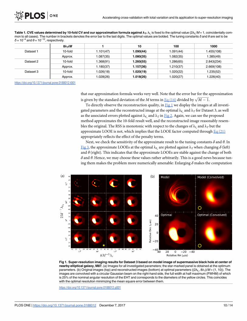
To directly observe the reconstruction quality, in Fig 1 we display the images at all investi-
gated parameters and the reconstructed image at the optimal λℓ1and λT for Dataset 3, as well
as the associated errors plotted against λℓ1and λT in Fig 2. Again, we can see the proposed
method approximates the 10-fold result well, and the reconstructed image reasonably resem-
bles the original. The RSS is monotonic with respect to the changes of λl1 and λT but the
approximate LOOE is not, which implies that the LOOE factor computed through Eq (21)
appropriately reflects the effect of the penalty terms.
Next, we check the sensitivity of the approximate result to the tuning constants δ and θ. In
Fig 3, the approximate LOOEs at the optimal λℓ1are plotted against λT when changing δ (left)
and θ (right). This indicates that the approximate LOOEs are stable against the change of both
δ and θ. Hence, we may choose these values rather arbitrarily. This is a good news because tun-
ing them makes the problem more numerically amenable: Enlarging δmakes the computation
Table 1. CVE values determined by 10-fold CV and our approximation formula against λT. λℓ1 is fixed to the optimal value (2λℓ1/M = 1, coincidentally com-
mon to all cases). The number in brackets denotes the error bar to the last digits. The optimal values are bolded. The tuning constants δ and θ are set to be
δ = 10−4 and θ = 10−12, respectively.
8λT/M 1 10 100 1000
Dataset 1 10-fold 1.101(47) 1.090(44) 1.091(44) 1.455(108)
Approx. 1.087(35) 1.080(35) 1.082(35) 1.385(49)
Dataset 2 10-fold 1.368(91) 1.260(55) 1.286(65) 2.843(234)
Approx. 1.180(37) 1.157(36) 1.210(37) 2.669(108)
Dataset 3 10-fold 1.026(18) 1.020(19) 1.020(22) 1.235(52)
Approx. 1.028(26) 1.018(26) 1.020(27) 1.226(40)
https://doi.org/10.1371/journal.pone.0188012.t001
Fig 1. Super-resolution imaging results for Dataset 3 based on model image of supermassive black hole at center of
nearby elliptical galaxy, M87. (a) Images for all investigated parameters; the star-marked panel is obtained at the optimum
parameters. (b) Original images (top) and reconstructed images (bottom) at optimal parameters ((2λℓ1, 8λT)/M = (1, 10)). The
images are convolved with a circular Gaussian beam on the right-hand side, the full width at half maximum (FWHM) of which
is 25% of the nominal angular resolution of the EHT and corresponds to the diameters of the yellow circles. This coincides
with the optimal resolution minimizing the mean square error between them.
https://doi.org/10.1371/journal.pone.0188012.g001
Accelerating cross-validation with total variation and its application to super-resolution imaging
PLOS ONE | https://doi.org/10.1371/journal.pone.0188012 December 7, 2017 10 / 14

of the Hessian inversion more numerically stable; increasing θ lowers the effective degrees of
freedom. The second property associated with θ is really beneficial when treating a large-size
dataset, because it can downsize the Hessian and reduce the cost for computing its matrix
inversion. In Table 2, the values of the effective degrees of freedom are given when changing θ.
The reduction of the degree of freedom at large (yet small enough compared to δ = 10−4) θ is
significant, which encourages us to apply the proposed formula to larger-size datasets.
Finally, let us see the data-size dependence of the approximation accuracy and of the
computational cost for solving Eq (3) and for obtaining the approximate LOOE from the solu-
tion. The data analyzed here is an identical simulated image of black hole expressed with dif-
ferent number of pixels. When solving Eq (3), we used Intel(R) Core(TM) i7-5820K CPU of
3.30GHz with 6 cores for N = 502 = 2500 and Intel(R) Xeon(R) CPU E5-2699 v3 of 2.30GHz
with 36 cores for N = 1002 and 1502, and employed an algorithm called “MFISTA” proposed in
[8, 9]. Meanwhile, we used a laptop of a 1.7 GHz Intel Core i7 with two CPUs for evaluating
Fig 2. (a) 3D plot of mean CVEs against λℓ1 and λT without error bars. (b) Plot of mean CVEs and RSS against λT at the optimal value of λℓ1, 2λℓ1/M = 1. (c)
Plot of mean CVEs and RSS against λℓ1 at the optimal value of λT, 8λT/M = 10. For (c), the RSS is overlapped with the CVEs in the symbol size. In all the
cases, the agreement between the approximate LOOE and the 10-fold CVE is fairly good. The tuning constants δ and θ are set to be δ = 10−4 and
θ = 10−12, respectively.
https://doi.org/10.1371/journal.pone.0188012.g002
Fig 3. Comparative plots of mean approximate LOOEs against λT at 2M−1 λℓ1= 1 when (a) δ changes as 10−6–10−3 with fixed θ = 10−12; (b) θ
changes as 10−12–10−6 with fixed δ = 10−4. They show that the LOOE curves are rather stable against the choice of the tuning constants.
https://doi.org/10.1371/journal.pone.0188012.g003
Accelerating cross-validation with total variation and its application to super-resolution imaging
PLOS ONE | https://doi.org/10.1371/journal.pone.0188012 December 7, 2017 11 / 14

the approximate LOOE. Hence the comparison is not fair and unfavorable to the approxima-
tion formula. The left panel indicates that the approximation accuracy becomes better for
larger sizes. This is reasonable because the perturbation we have employed should have better
accuracy as the model and data become larger, though the accuracy at N = 502 = 2500 is already
good. The right panel clearly shows the advantage of the developed formula: The actual
computational time of the approximate LOOE is significantly shorter than that of the algo-
rithm convergence for solving Eq (3) in the investigated range of system sizes, even under the
unfair comparison mentioned above. However, this advantage will be less prominent if the
model becomes very large: Our approximation formula needs the Hessian inversion whose
computational cost is scaled as O((|C| + |SI|)3)� O(N3), while MFISTA requires the cost of
O(N2) as long as the number of steps to convergence is constant against N. The crossover size
at which these two computational costs become comparable is roughly estimated as N� 106,
though such crossover tendency cannot be seen yet from Fig 4. For such large systems, a new
fundamental solution should be tailored to resolve the computational-cost problem, though
tuning θ to a large value in the present method can still be a good first aide.
7 Conclusion
In this paper, we have developed an approximation formula for the CVE of a sparse linear
regression penalized by ℓ1 and TV terms, and demonstrated its usefulness in the reconstruc-
tion of simulated black hole images. Our derivation is based on the perturbation assuming
the small difference between the full and leave-one-out solutions. This assumption will not be
fulfilled for some specific cases, i.e. when the measurement matrix is sparse. However, for
most of dense measurement matrices, such as the Fourier matrix discussed in this paper, our
Table 2. The effective degrees of freedom j~SIþZ j, the number of clusters + the number of isolated variables, against θ for Dataset 3 at δ = 10−4 and
the optimal parameters (2λℓ1, 8λT)/M = (1, 10).
θ 1e-12 1e-11 1e-10 1e-09 1e-08 1e-07 1e-06
j~SIþZj 5733 5524 5243 4814 4112 2922 1408
https://doi.org/10.1371/journal.pone.0188012.t002
Fig 4. (a) Plot of mean CVEs at optimal parameters of different sizes. (b) Log-log plot of the computational times for solving the optimization
problem (3) and for obtaining the approximate value of CVE against the size of datasets.
https://doi.org/10.1371/journal.pone.0188012.g004
Accelerating cross-validation with total variation and its application to super-resolution imaging
PLOS ONE | https://doi.org/10.1371/journal.pone.0188012 December 7, 2017 12 / 14

assumption will be reasonably satisfied. Hence we expect the range of application of our for-
mula is wide enough and we would like encourage the readers to use this formula in their own
work. It is also straightforward to generalize the developed formula to other types of TV, and
two examples of the generalization for the anisotropic and square TVs have been explained.
The key concept of our formula, perturbation between the LOO and full systems, is very
general and can be applied to more general statistical models and inference frameworks [23].
The development of practical formulas for those cases will facilitate higher levels of modeling
and computation.
Acknowledgments
We would like to express our sincere gratitude to Mareki Honma and Fumie Tazaki for their
helpful discussions. We thank Katherine L. Bouman for preparing the EHT Imaging Challenge
website [22, 24]. We also thank Andrew Chael and Lindy Blackburn for writing a simulation
software to produce sample data sets [25].
Author Contributions
Conceptualization: Yoshiyuki Kabashima.
Data curation: Shiro Ikeda, Kazunori Akiyama.
Formal analysis: Tomoyuki Obuchi, Yoshiyuki Kabashima.
Funding acquisition: Tomoyuki Obuchi, Shiro Ikeda, Kazunori Akiyama, Yoshiyuki
Kabashima.
Investigation: Tomoyuki Obuchi.
Methodology: Tomoyuki Obuchi, Yoshiyuki Kabashima.
Project administration: Shiro Ikeda, Yoshiyuki Kabashima.
Software: Shiro Ikeda.
Validation: Tomoyuki Obuchi.
Visualization: Tomoyuki Obuchi, Kazunori Akiyama.
Writing – original draft: Tomoyuki Obuchi.
Writing – review & editing: Tomoyuki Obuchi.
References1. Rish I, Grabarnik G. Sparse Modeling: Theory, Algorithms, and Applications. CRC Press; 2014.
2. Hastie T, Tibshirani R, Wainwright M. Statistical Learning with Sparsity: The Lasso and Generalizations.
CRC Press; 2015.
3. http://sparse-modeling.jp/index_e.html
4. Mairal J, Bach F, Ponce J. Sparse modeling for image and vision processing. Available from:
arXiv:1411.3230v2.
5. Tibshirani R. Regression shrinkage and selection via the lasso. J. Royal. Statist. Soc. B., 58, 267
(1996).
6. Efron B, Hastie T, Johnstone I, Tibshirani R. Least angle regression. Ann. Stat., 32, 407 (2004). https://
doi.org/10.1214/009053604000000067
7. Rudin L I, Osher S, Fatemi E. Nonlinear total variation based noise removal algorithms. Physica D 60,
259 (1992). https://doi.org/10.1016/0167-2789(92)90242-F
8. Chambolle A. An algorithm for total variation minimization and applications. J. Math. Imaging Vision,
20, 89 (2004). https://doi.org/10.1023/B:JMIV.0000011321.19549.88
Accelerating cross-validation with total variation and its application to super-resolution imaging
PLOS ONE | https://doi.org/10.1371/journal.pone.0188012 December 7, 2017 13 / 14

9. Beck A, Teboulle M, Fast gradient-based algorithms for constrained total variation image denoising and
deblurring problems. IEEE Trans. Image Process., 18, 2419 (2009). https://doi.org/10.1109/TIP.2009.
2028250 PMID: 19635705
10. Obuchi T, Kabashima Y. Cross validation in LASSO and its acceleration. J. Stat. Mech., 053304 (2016).
https://doi.org/10.1088/1742-5468/2016/05/053304
11. http://www.eventhorizontelescope.org
12. Asada K, Kino M, Honma M, Hirota T, Lu R.-S, Inoue M. White Paper on East Asian Vision for mm/
submm VLBI: Toward Black Hole Astrophysics down to Angular Resolution of 1 RS, arXiv:1705.04776
13. Akiyama K, Lu R, Fish V L, Doeleman S S, Broderick A E, Dexter J, et al. 230 GHz VLBI observations of
M87: Event-horizon-scale structure during an enhanced very-high-energy γ-ray state in 2012. Astro-
phys. J., 807, 150 (2015). https://doi.org/10.1088/0004-637X/807/2/150
14. Chan T F, Osher S, Shen J. The Digital TV Filter and Nonlinear Denoising, IEEE Trans. Image Process.,
10, 231 (2001). https://doi.org/10.1109/83.902288 PMID: 18249614
15. Wiaux Y, Jacques L, Puy G, Scaife A M M, Vandergheynst P. Compressed sensing imaging techniques
for radio interferometry. Mon. Not. R. Astron. Soc., 395, 1733 (2009). https://doi.org/10.1111/j.1365-
2966.2009.14665.x
16. Li F, Cornwell T J, de Hoog F. The application of compressive sampling to radio astronomy I. Deconvo-
lution. A&A, 528, A31 (2011).
17. Honma M, Akiyama K, Uemura M, Ikeda S. Super-resolution imaging with radio interferometry using
sparse modeling. Publ. Astron. Soc. Japan, 66, 1 (2014). https://doi.org/10.1093/pasj/psu070
18. Honma M, Akiyama K, Tazaki F, Kuramochi K, Ikeda S, Hada K et al. Imaging black holes with sparse
modeling. JPCS, 699, 012006 (2016).
19. Ikeda S, Tazaki F, Akiyama K, Hada K. PRECL: A new method for interferometry imaging from closure
phase. Publ. Astron. Soc. Japan, 68, 45 (2016). https://doi.org/10.1093/pasj/psw042
20. Akiyama K, Ikeda S, Pleau M, Fish V, Tazaki F, Kuramochi K et al. Superresolution Full-polarimetric
Imaging for Radio Interferometry with Sparse Modeling. The Astronomical Journal, 153, 1 (2017).
https://doi.org/10.3847/1538-3881/aa6302
21. Akiyama K, Kuramochi K, Ikeda S, Fish V, Tazaki F, Honma M et al. Imaging the Schwarzschild-radius-
scale Structure of M87 with the Event Horizon Telescope Using Sparse Modeling. The Astrophysical
Journal, 838, 1 (2017). https://doi.org/10.3847/1538-4357/aa6305
22. http://vlbiimaging.csail.mit.edu/imagingchallenge
23. Kabashima Y, Obuchi T, Uemura M, Approximate cross–validation formula for Bayesian linear regres-
sion. Available from arXiv:1610.07733.
24. Bouman K L, Johnson M D, Zoran D, Fish V L, Doeleman S S, Freeman W T. Computational Imaging
for VLBI Image Reconstruction. The IEEE Conference on Computer Vision and Pattern Recognition,
913 (2016).
25. Chael A A, Johnson M D, Narayan R, Doeleman S S, Wardle J F C, Bouman K L. High-resolution Linear
Polarimetric Imaging for the Event Horizon Telescope. The Astrophysical Journal, 829, 15 (2016).
https://doi.org/10.3847/0004-637X/829/1/11
Accelerating cross-validation with total variation and its application to super-resolution imaging
PLOS ONE | https://doi.org/10.1371/journal.pone.0188012 December 7, 2017 14 / 14