Embed Size (px)
Citation preview
Bachelor thesisComputer Science
Radboud University
Accelerating BCCD using parallelcomputing
Author:
Ties Robroek
s4388615
First supervisor/assessor:
prof. dr. T.M. (Tom) Heskes
Second supervisor:
Dr Fabian Gieseke
Second assessor:
dr.ir. T. (Tom) Claassen
[email protected] 16, 2016

Abstract
The BCCD algorithm is powerful yet computationally intensive. Even though
it is highly accurate, its speed prevents the processing of larger datasets.
High-performance computing solutions such as CUDA boast with massive
potential speed boosts. Can high-performance computing increase the speed
of BCCD to overcome the time obstruction? This thesis describes the con-
version process from source code to CUDA kernel in detail. The product is
a CUDA kernel that can handle exponentially larger datasets.
Contents
1 Introduction 3
2 Preliminaries 5
3 Research 9
3.1 Review original MATLAB version . . . . . . . . . . . . . . . 9
3.2 Target function . . . . . . . . . . . . . . . . . . . . . . . . . . 11
3.3 The function . . . . . . . . . . . . . . . . . . . . . . . . . . . 13
3.4 Translate into Python . . . . . . . . . . . . . . . . . . . . . . 14
3.4.1 Initialization . . . . . . . . . . . . . . . . . . . . . . . 14
3.4.2 Structure loop . . . . . . . . . . . . . . . . . . . . . . 14
3.4.3 Resolve . . . . . . . . . . . . . . . . . . . . . . . . . . 15
3.5 Improving upon the original Python version . . . . . . . . . . 15
3.6 Translate to C empowered Python (SWIG) . . . . . . . . . . 17
3.6.1 The Find function . . . . . . . . . . . . . . . . . . . . 18
3.6.2 Determinants . . . . . . . . . . . . . . . . . . . . . . . 21
3.6.3 Interfacing using SWIG . . . . . . . . . . . . . . . . . 22
3.7 CUDA . . . . . . . . . . . . . . . . . . . . . . . . . . . . . . . 22
3.8 Speeding up CUDA . . . . . . . . . . . . . . . . . . . . . . . 23
3.8.1 Shared memory . . . . . . . . . . . . . . . . . . . . . . 23
3.8.2 Single-precision CUDA . . . . . . . . . . . . . . . . . . 24
3.8.3 The log() function . . . . . . . . . . . . . . . . . . . . 24
3.9 Results . . . . . . . . . . . . . . . . . . . . . . . . . . . . . . . 25
3.10 Overhead . . . . . . . . . . . . . . . . . . . . . . . . . . . . . 29
4 Related Work 30
1
5 Conclusions 31
A Appendix 33
A.1 A: Hardware specifications . . . . . . . . . . . . . . . . . . . . 33
A.2 B: Double-precision CUDA kernel . . . . . . . . . . . . . . . . 37
2
Chapter 1
Introduction
The BCCD algorithm, short for Bayesian Constraint-Based Causal Discov-
ery algorithm, provides an excellent way to generate causal networks. With
this algorithm the robustness of a Bayesian approach is combined with the
power of a constraint-based approach. Bayesian scores are based on a large
data input. These scores are then refined via reliability testing. This makes
the BCCD algorithm powerful in terms of accuracy. [2] Introducing larger
datasets, however, reveals a large issue. A vast amount of input results in a
large or detailed amount of output. As all input needs to be processed, the
time-complexity skyrockets on large datasets. This seriously limits the prac-
tical use of the algorithm, as application on large datasets would be ideal in
most circumstances. This large amount of time-complexity thus limits the
use of the current BCCD implementation to small datasets. [9]
To increase the size of applicable datasets the time-complexity of the al-
gorithm needs to decrease. This can usually be done via two ways; either the
code is made more efficient or the code utilises more computing power. The
latter can be achieved using GPU computing. GPU computing is a rapidly
growing field in computer science. [7] Not only are GPUs used to dra-
matically enhance computer visual performance, GPUs are also increasingly
common as a way to calculate with high performance. [8] If implemented
efficiently, GPUs greatly outperform similarly priced CPU systems. [10].
GPU computing thus opens up as a possible solution to the BCCD algo-
rithm. The computational force mustered by GPUs may be able to reduce
3
the time constraints hampering the effective use of the algorithm [7]. This
leads to the following research question: Does GPU computing increase the
computational speed of the BCCD algorithm in an effective way?
The research questions can be split up using the following sub-questions:
1. How do we parallelize the BCCD algorithm using GPUs?
2. What kind of speed-up can be achieved using this parallelization?
3. Keeping the additional overhead caused by the implementation in
mind, how effective is found speed-up?
4
Chapter 2
Preliminaries
Parallel computing is a form of High Performance computing. By using the
strength of many smaller computational units, parallel computing can pro-
vide a massive speed boost for traditional algorithms.[3] There are multiple
programming solutions that offer parallel computing.
Traditionally, programs are written to be executed linearly. Languages
such as COBOL or FORTRAN have been designed for this linear execution.
The hardware at the time did only support this linear execution. Due to
this heritage, most of the programs that are written today still hold true to
this linear type of execution.
With the evolution of hardware, processors have started to support mul-
tiple mathematical units. These so called ”cores” allow basic parallelism
to be used in traditional code. Programmes can be written in such a way
that actions can be performed simultaneously; greatly improving the execu-
tion time of the program. This technique is referred to as ”threading” and
describes executing multiple ”threads” (code executors) at the same time.
Processors have seen many improvements over time. Threading has
caused a massive increase in performance for high-throughput mathematical
operations. Steadily more and more transistors have found their place on
processor chips. By increasing the transistor density the processors have
massively increased in power.[10] All these improvements have not had any
impact on usability. Processors, as central manager of the computer, have
a large amount of control and autonomy over the hardware. The managing
5
effectiveness of the processor has only seen increase over time and has con-
tributed even more to it’s massive flexibility. Higher-level languages have
become highly developed and popular, making programming easier than
ever. This causes the programming of the processor, which most program-
ming is categorized as, to be by far the most popular and practised type of
programming.
More recently, parallel computing has steadily become more popular.
Where for a long amount of time the power of a computer was upgraded by
increasing the computing efficiency or the transistor density of the proces-
sor, newer systems sport more cores. This causes units to be more powerful,
but also rely more on correctly threaded applications. New challenges in the
hardware design field such as heat generation restrictions have also boosted
the research into these systems. Running multiple computational units was
previously frowned upon due to the increase in development complexity.
Nowadays, most modern computers have at least two computational units
in their processor. With the current boom in mobile hardware the develop-
ment wave has been fronted by the development of low power multiple core
processors. Devices such as mobile phones and tablets use these processors
instead of the more traditional linear systems. The accurate division of tasks
between the cores saves a monumental amount of power and greatly reduces
the generation of heat. These characteristics were later found to be useful
in what some may find unexpected other fields. The new Japanese exascale
supercomputer manufactured by Fujitsi is rumoured to use ARM products,
which is the leading developer on mobile processors.
At the heart of parallel computing is perhaps the Graphics Processing
Unit. The GPU has been in development since the 1970s. Contrary to the
processor, the graphics chip has been designed to work parallel from the
start. This makes the GPU in design much more capable to fully utilize the
advantages of parallel programmed algorithms.[7]
When using GPU’s, parallel computing becomes a form of High Perfor-
mance computing. GPU’s have a much larger amount of cores than pro-
cessors by design. By using the strength of many smaller computational
units, parallel computing can provide a massive speed boost for traditional
algorithms. There are multiple programming solutions that offer parallel
6
computing. CUDA was chosen as programming language for this research.
CUDA, Compute Unified Device Architecture, is a powerful environ-
ment that, when implemented correctly, can drastically increase the compu-
tational power available to an algorithm. To be able to implement CUDA
effectively, however, the algorithm should be structured in a peculiar way.
When working with devices such as graphical processing units, all informa-
tion to be processed must be made accessible for these units. This means
that the CUDA languages, as well as other GPU empowered programming
languages, are highly subject to large memory allocation operations. As
the final goal of speeding up the BCCD algorithm is to be able to pro-
cess larger amounts of data, these memory allocation operations become
very demanding.[9] This is why it is absolutely essential to restructure the
BCCD algorithm in such a way that the memory allocations are performed
optimally.
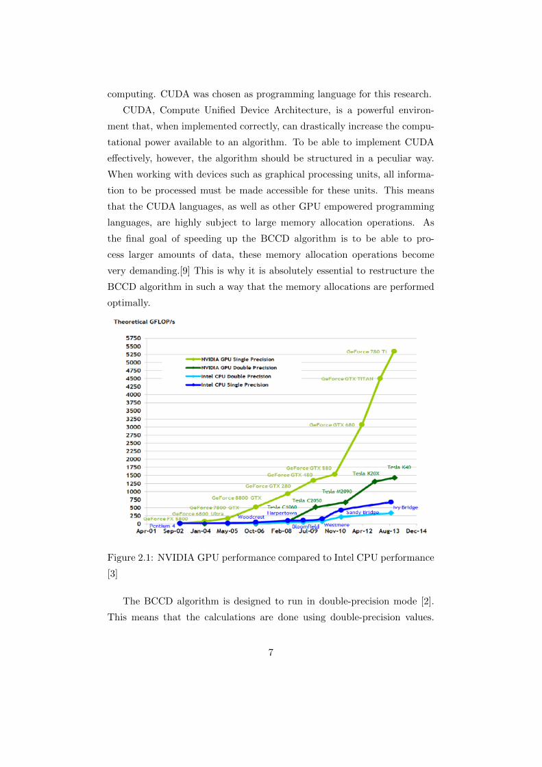
Figure 2.1: NVIDIA GPU performance compared to Intel CPU performance
[3]
The BCCD algorithm is designed to run in double-precision mode [2].
This means that the calculations are done using double-precision values.
7
This ensures correct data handling for very accurate computations. GPU’s
however tend to perform much more efficiently in single-precision mode.
Converting double-precision values to single-precision values is not a hazard-
less process. The loss in precision can cause corruption or inaccuracy in
execution results. Once the BCCD algorithm has been translated to a CUDA
function, a single-precision CUDA function could be attempted.
8
Chapter 3
Research
The translation of the BCCD algorithm to a high performance parallelized
approach has been broken down to the following steps on which this research
is structured:
1. Review original MATLAB version
2. Translate to Python
3. Translate to C empowered Python (SWIG)
4. Translate to CUDA
5. High performance enhancements
3.1 Review original MATLAB version
The original version of the BCCD algorithm, as fabricated by Heskes and
Claassen [2], has been written in MATLAB. MATLAB is a programming
language developed by MathWorks that provides an user friendly and effec-
tive workspace for scientific research. MATLAB, however, is not optimized
for speed [9]. Following the research question the goal of this research is im-
proving the speed of the algorithm using different programming techniques.
The BCCD algorithm is a multi-stage algorithm. The following stages
are distinguished:
• Stage 0: Mapping
9
• Stage 1: Search
• Stage 2: Inference
In terms of the MATLAB code, Stage 0 is referenced to as ”initializa-
tion”, and stage 2 as ”aftercare”. In order to implement a faster version,
it is essential to assess the speed of the current code per stage. The stage
that performs the slowest will be the focal point. Improving on this stage
will yield the greatest return. This stage will from now on be referenced to
as ”bottleneck stage”.
As previously documented, the algorithm supposedly performs well enough
on simple datasets. The datasets supplied are randomly generated multi-
variate gaussian model datasets with 10 variables. Increasing the amount
of variables, however, quickly deteriorates the speed at which the algorithm
can complete its task. This means that, to identify the correct bottleneck
stage, a complex dataset has to be used. The worst scaling stage will at
this point project a heavy dropoff in speed. To ascertain the projection of
this trend to even more complex datasets, the duration of the tests will be
compared to those of easier tests (less complex datasets).
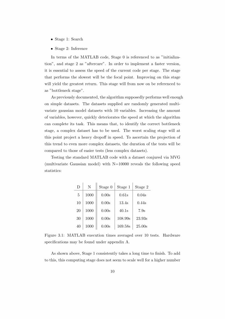
Testing the standard MATLAB code with a dataset conjured via MVG
(multivariate Gaussian model) with N=10000 reveals the following speed
statistics:
D N Stage 0 Stage 1 Stage 2
5 1000 0.00s 0.61s 0.04s
10 1000 0.00s 13.4s 0.44s
20 1000 0.00s 40.1s 7.9s
30 1000 0.00s 108.99s 23.93s
40 1000 0.00s 169.58s 25.00s
Figure 3.1: MATLAB execution times averaged over 10 tests. Hardware
specifications may be found under appendix A.
As shown above, Stage 1 consistently takes a long time to finish. To add
to this, this computing stage does not seem to scale well for a higher number
10
D. Due to these properties, this research will focus on accelerating this part
of the algorithm.
The next step is to isolate the code responsible for the execution of this
stage. When looking at the original MATLAB code, a host of functions are
called in order to fulfil this step. However, when looking at the execution
times, a majority of the time the following function is being called:
GetBayesianProbability_Per_Structure_BGe
Due to the bottleneck created by this function, all attempts to improve
the performance of the algorithm will be focused on this piece of code. It
should be noted that, if any increase in performance is realised, this increase
in performance will never be able to make the code instant. The performance
increase will never be able to exceed the theoretical performance of the code
when this function is instantaneous. All other functions are not altered in
any way.
3.2 Target function
Python is a programming language well known for it’s modularity and adapt-
ability. Python shares many similarities with MATLAB, which allows it to
be translated to relatively easily. Due to the modularity of Python and
it’s many possibilities, a Python version can be readily adapted for higher
performance computing. This, together with the translation ease between
the two languages, makes it an incredibly strong language to base future
implementations on.
Pythons similarity to MATLAB is a huge convenience for the translation.
Future translation to higher performing solutions will surface multiple issues.
Usually, functions cannot be translated directly from MATLAB to lower
level languages such as C. These languages, however, are unavoidable in
order to conceive a fast algorithm. Python, however, is a very high level
language and shared this characteristic with MATLAB. For most MATLAB
functions a suitable Python replacement is present. In order to bridge to
higher performance solutions, the next step is to make a Python version of
11
the algorithm. Once a Python version has been realised, Pythons modularity
can be used to create better performing versions.
As only stage 1 (Search) will be translated to high-performance code, an
interface has to be realised between the MATLAB version and any future
versions. Any future versions will be called by a Python interface. The
connection between MATLAB and future versions should thus be done by
transferring the MATLAB data to a Python environment.
A ready-made solution to provide the correct environment for new ver-
sions of the algorithm is the so called exporting of the MATLAB workspace.
When running any MATLAB code, any variables and values are stored and
referenced in the ”workspace”. This workspace, combined with the execu-
tion pointer, provide all required information to run a MATLAB algorithm.
Due to these characteristics, a logical bridge between Python and MAT-
LAB would be exporting the MATLAB workspace and loading this into
Python. On MATLABs end this can be realised by using the export func-
tion
save(filename, variables);
which directly exports all listed variables of the workspace into a file. It
should be noted that the save function may be called without specifying
which variables have to be exported. In this case, the whole workspace is
exported into the file. For this purpose, though, the variables will be speci-
fied, as not the whole workspace is required to run the algorithm. Only the
variables required by the original MATLAB function call will be exported:
GetBayesianProbability_per_Structure_BGe(C,N,alpha_mu,T,alpha_w,SS,prS)
• C = covariance/correlation matrix
• N = nr. of data records in C
• alpha mu = prior weight on precision matrix for mean
• T = parametric matrix in Wishart
• alpha w = degrees of freedom in Wishart > (D-1)
• SS = array of structures size(C)
12
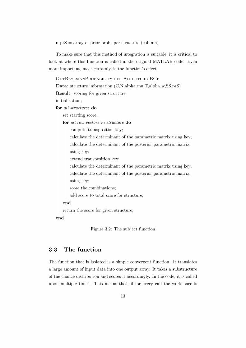
• prS = array of prior prob. per structure (column)
To make sure that this method of integration is suitable, it is critical to
look at where this function is called in the original MATLAB code. Even
more important, most certainly, is the function’s effect.
GetBayesianProbability per Structure BGe
Data: structure information (C,N,alpha mu,T,alpha w,SS,prS)
Result: scoring for given structure
initialization;
for all structures do
set starting score;
for all row vectors in structure do
compute transposition key;
calculate the determinant of the parametric matrix using key;
calculate the determinant of the posterior parametric matrix
using key;
extend transposition key;
calculate the determinant of the parametric matrix using key;
calculate the determinant of the posterior parametric matrix
using key;
score the combinations;
add score to total score for structure;
end
return the score for given structure;
end
Figure 3.2: The subject function
3.3 The function
The function that is isolated is a simple convergent function. It translates
a large amount of input data into one output array. It takes a substructure
of the chance distribution and scores it accordingly. In the code, it is called
upon multiple times. This means that, if for every call the workspace is
13
exported to an individual file, multiple files will have to be read to interface
correctly with any future implementations.
3.4 Translate into Python
In order to translate the function correctly into Python, a piece of Python
script has to be written that loads the workspace values. The popular sci-
entific calculation package Scipy provides a simple yet effective solution for
this. The Scipy input-output (Scipy.io) function
loadmat(filename);
loads the workspace data into the memory. The data is stored in the stan-
dard Python List format. Individual pieces of data can be retrieved by
calling their identifier.
Once the workspace is loaded into memory, all values can be easily ac-
cessed. Due to the high level structure Python has similar to MATLAB,
most translation steps are fairly straightforward. This process is hereby
described per part of the function:
3.4.1 Initialization
In the initialization part of the function, many of the input values are rear-
ranged. The posterior parametric matrix R is computed and the arrays are
initialized. The code in this section can be translated to Python without
too much hassle. Handling the data is done by using the Python package
Numpy. This package allows more advanced data manipulation. Numpy
introduces Numpy arrays. This is the format the workspace data is im-
ported in into Python using ”loadmat()”. Numpy will also provide future
advantages in regards to interfacing with the C and CUDA versions of the
code.
3.4.2 Structure loop
The structure loop consists of a double for-loop. These loop over all struc-
tures and variables inside these structures. Every structure is scored using
14
a formula consisting of four scoring values. Every scoring value is computed
by computing the determinant of a substructure. The algorithm uses the
logarithm of these determinant values in order to preserve efficiency. MAT-
LAB has set functions for these operations, namely ”log()” and ”det()”.
These functions are standard to the MATLAB library. Python, however,
does not natively support these functionalities. In order to be able to per-
form these operations without having to define new functions to do so,
Numpy is used again. Numpy provides the functions ”numpy.log()” and
”numpy.linalg.det()” which behave similar to their MATLAB counterparts.
Another important function is the MATLAB function ”find()”. This func-
tion is utilized here to form the vector for substructures that have to be
analysed. These substructures are formulated using a vector which pre-
scribes what rows and columns are to be used. A solution to translate this
into Python can be found in the Numpy function ”numpy.nonzero()”. Both
functions can be used to list the non-empty elements of a vector. This vector
is then used to form the substructure in MATLAB by referencing the vector
to the original structure matrix. MATLAB will return the substructure in
this case. This does not translate directly to Python. Numpy, however, has
the function ”np.ix ()” which can be used for the same result.
3.4.3 Resolve
This fase only consists of a few lines of code. It can be as easily translated
as the Initialization phase.
3.5 Improving upon the original Python version
Even though this first Python function is functional, it is far from practi-
cal. This practicality is absent in both the performance perspective and the
research perspective. The new version of the algorithm performs noticeably
worse than the original MATLAB version. This can likely be attributed to
the code structure being written to perform well in MATLAB. The transla-
tion is rough-edged and is not optimized in Pythons favour. From a research
perspective, the code can still very much be improved. The Python script
is written from a very high level. Libraries such as Numpy are necessary for
15
a correct execution. They provide invaluable support to bridge the Python
version to the original MATLAB code. The computationally intensive part,
however, depends on function calls from this library to high degree. These
function calls are practical to ease the translation from MATLAB code to
Python code. When the Python code has to be translated into a script
in a lower level language such as C, these functions lose a large amount of
appeal. For example, C does not have a practical library to provide an easy
yet effective parallel to the ”numpy.det()” function. Once a C version has
to be realised, this determinant function has to be written in C. Higher level
languages such as Python are more flexible. By first writing the determi-
nant function as a separate function in Python, the gap between the Numpy
source implementation and the C function is made considerably smaller.
Before a new Python function can be realised, it is important to look
at the environment the function is called in. The aim of this research is
to provide a high-performing result. This means that, for this function,
an implementation is preferred that performs optimally. In the algorithm,
the determinant function is called to compute a determinant of a matrix of
selected sizes. The size varies between a 0x0 matrix and a 5x5 matrix. To
determine the determinant of a matrix the Laplace formula may be used.
This formula is only practical for matrices larger than 2x2. Using the Laplace
formula, the determinant is expressed in terms of it’s minor, via:
det(A) =n∑
j=1(−1)i+jai,jMi,j
Where:
• A: The original matrix
• n: The size of the original matrix
• i: ith row
• j: jth column
• Mi,j : The determinant of the (n-1)(n-1)-submatrix that results from
A by removing i and j
16
• Ai,j : The value at (i,j) in the original matrix A
The Laplace formula provides a solid way to find a determinant for any
larger matrix. The formula is recursive, however, so when utilizing this
formula some base cases have to be defined.
• The determinant of a 0x0 matrix is defined to be 1.
• The determinant of an 1x1 matrix is it’s only value: M0,0.
• The determinant of a 2x2 matrix is defined by the following formula:∣∣∣∣∣∣a b
c d
∣∣∣∣∣∣ = ad− bc
The determinant of a 3x3 matrix can be calculated using the Laplace
formula. The definition of the determinant of a 2x2 matrix can be used to
solve the equation. This approach, however, requires an unnecessarily large
amount of operations. An extention of the 2x2 matrix definition can be
used to calculate the determinant on 3x3 matrices more efficiently. The rule
of Sarrus provides a more compact and usable solution to compute a 3x3
matrix: ∣∣∣∣∣∣∣∣∣a b c
d e f
g h i
∣∣∣∣∣∣∣∣∣ = aei + bfg + cdh− gec− hfa− idb
A combination of the Laplace formula and the Rule of Sarrus covers any
matrix larger than 2x2. The newly implemented Python function will thus
utilize this to compute the determinants for these matrices. Any smaller
matrix will have it’s determinant derived from the listed definitions.
3.6 Translate to C empowered Python (SWIG)
Although the Python version performed marginally better than the MAT-
LAB version, it is yet not on to par in terms of speed. To be able to achieve
17
higher speeds PyCuda will be implemented. This is a library for Python
that allows for Python to call strong, fast CUDA kernels. These kernels are
capable of achieving massive speed; even an initial version may very well out-
perform the original Python code. Python does not share many similarities
with this kernel code, however, thus making the conversion difficult. Using
a middle ground may ease the translation process. This is where SWIG,
Simplified Wrapper and interface Generator, comes into play. SWIG is a
powerful tool that allows the user to write a Python extension module in C.
These have two important advantages over normal Python code:
1. C code is much faster than Python code, thus delivering a speed-up.
2. C code much more closely resembles CUDA code, which eases later
translation steps.
There are, also, caveats to be taken into consideration:
1. C is a lower level language than Python. Many operations that have
pre-built functions in Python have to be programmed from scratch in
the C language.
2. The C function will be called within Python. The interfacing between
the Python and the C part has to be done well in order to make the
resulting code efficient.
The improved Python version greatly decreases the effort gap between
a Python version and a SWIG C version. The code that has to be trans-
lated can now largely be translated directly into C code using correct SWIG
interfacing.
3.6.1 The Find function
One of the most important abstractions between Python and C is the use
of pointers. Python does not work with pointers. Any value accessing is
done via cataloguing and variables. The Python data structure ”dictionary”
is a great example of this. This structure holds a list of labelled values.
These labels, so called ”keys”, may be referenced to access underlying values.
Structures like these highly contribute to the high-level nature Python has.
18
C does not have such a structure and instead uses a lower-level approach.
This will have several implications for the C code. The two loops and their
accompanied calculations require a handful of values to perform. Due to
the nature of the algorithm, a large amount of the information required
comes in the form of one- and two-dimensional data structures. Numpy
arrays are used to both represent the structure that is being analysed and
the array of scoring factors. These will all be translated to one dimensional
data structures in C. An example is given below for the following Python
structure:
matrix[i,j];
This details an Numpy array with size i, j. The C representation of this
structure will be:
matrix[i*j];
In contrary to the Python version, the C version accesses the whole array
via one index. All values are indexed as one large row of items. In this
example, indexes [0 - i-1] will reference the first row of the Numpy array.
The second row of the Numpy array can be accessed using the indexes [i -
2i-1], etcetera.
Perhaps the most important data accesses are those to the substructures.
These substructures are defined by their row vectors. This is natively sup-
ported in MATLAB. In Python, the function ”numpy.ix ” could be used as
a substitute. C, however, does not provide a function for this. To be able to
realise this behaviour in C, a ”key vector” has to be generated. This struc-
ture is similar to the submatrix vector used in the MATLAB and Python
approaches. Any data access to the substructure is done via a ”key”. This
is an array that, for any required data access, points to the right value in
the main structure. Only one such key is needed for a submatrix; in the
original code the change in rows is identical to the change in columns. For
example, take the following key vector:
19
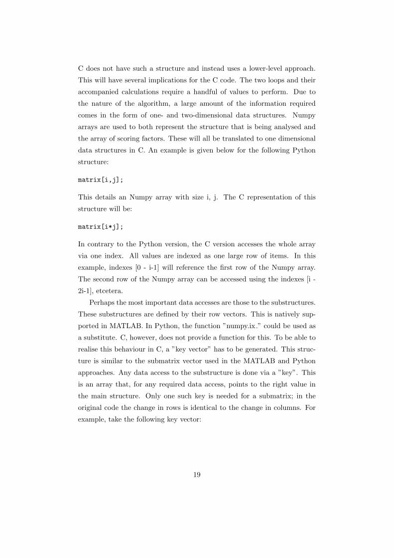
Index Value
0 1
1 2
2 4
When applied to the following structure:∣∣∣∣∣∣∣∣∣∣∣∣∣∣∣
a b c d e
f g h i j
k l m n o
p q r s t
u v w x y
∣∣∣∣∣∣∣∣∣∣∣∣∣∣∣Will result in the following substructure:∣∣∣∣∣∣∣∣∣
g h j
l m o
v w y
∣∣∣∣∣∣∣∣∣In the C code, this means that any time the substructure has to be
accessed, the primary structure is accessed instead via:
matrix[key[i + n * j]]
Translating the MATLAB version into a Python version gave us a simple
solution for the ”find()” call. This function is used to calculate submatrix
vector. Python provided a ready-made solution in the form of the Numpy
function ”numpy.nonzero()”. C does not have such a set function, though,
and to proceed a new C function has to be written. The function Find
follows the following behaviour:
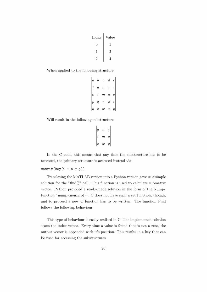
This type of behaviour is easily realised in C. The implemented solution
scans the index vector. Every time a value is found that is not a zero, the
output vector is appended with it’s position. This results in a key that can
be used for accessing the substructures.
20
Find
Data: Index vector)
Result: Submatrix key array
Take the index vector.
List the positions where there is a value present (!=0).
Return this list as an key vector.
Figure 3.3: The effect of the find() function
3.6.2 Determinants
As discussed before, C does not have a determinant function in it’s library.
Both MATLAB and Python do have one, although the latter requires the
package Numpy to do so. By creating a determinant function for the Python
version, the gap between the C implementation and the Python implemen-
tation has lessened. This makes the construction of a C version almost
trivial.
Only a few things have to be taken into account when translating the
Python determinant function into a C counterpart:
• The matrices have been flattened in C. This means that all the index-
ing has to be done via one dimension, as discussed earlier.
• The substructures are to be accessed via a key vector. The original
Python function has the substructure as a parameter. In the C version
the parameters will contain the original structure and the key vector.
All referencing has to be done via the key vector.
The determinant function written in Python was hard-coded for the first
four occurrences. This means that the first four cases are calculated directly.
The last two cases, 4x4 and 5x5 matrices, are computed via a recursive
relationship. This keeps the code compact, but increases the amount of
complexity for the system. In addition to the calculations, the computer
has to perform the function calls in order to compute the right result. This
is why, for the C version, a fully hard-coded approach has been chosen. This
means that, in addition to the previously hard-coded cases, the 4x4 and 5x5
solution has also been hardcoded. A generator has been written to generate
21
the code for these operations, as the code is lengthy and repetitive, making
it error-prone if coded by hand.
3.6.3 Interfacing using SWIG
After the discussed steps the C version is almost ready to go. The only
thing left is actually running the function using Python. SWIG (Simplified
Wrapper and Interface Generator) is used to achieve this. SWIG compiles
the specified C functions into Python extensions. These extensions can be
imported and called within Python.
3.7 CUDA
CUDA, Compute Unified Device Architecture, is a parallel computing plat-
form developed by NVIDIA. The platform is designed to work with C, C++
and FORTRAN. The translation of the algorithm to a CUDA capable ver-
sion can be easily achieved. The SWIG C version, being written in C, can be
translated to CUDA C without too much hassle. The specific interactions
required for SWIG are to be omitted and a few new interfacing actions have
to be assigned to enable the execution of such a version.
CUDA is a parallel computing platform. This means that, instead of
running the algorithm in a serial fashion, the algorithm should be inspected
for any possible parallelisms. Doing so may greatly increase the execution
speed. Multiple values could be computed simultaneously. CUDA performs
this parallel execution on the Graphics Processing Unit, GPU.
The function consists of two for-loops. The outer for-loop loops over
all structures, the inner for-loop over all substructures. The amount of
substructures is, for a given structure, equal to it’s size. This means that
a 5x5 matrix will see at most five repeats in this inner loop. The outer
loop, however, which specifies the amount of structures, may see a much
larger amount of repeats. The amount of structures analysed this way is
derived from the size of the structures. When computing on 5x5 matrices,
the amount of structures analysed will be 8728, the highest amount.
Comparing the size of both loops heavily opts that a parallelization on
the outer loop is the most logical, as it has the highest amounts of repeats.
22
Even though the algorithm is now written in a fast, parallel language, it is
far from truly optimized. In the next section a few methods to improve the
speed even more are discussed.
3.8 Speeding up CUDA
3.8.1 Shared memory
Algorithms programmed in a parallel way using CUDA may be fast, they
are not instant. Every year the hardware on which these algorithms can
be performed becomes more powerful. The raw computing force increases,
allowing for more threads to be executed in parallel. Nowadays the raw
computing power of the cores on this hardware is seldom the bottleneck for
most algorithms. The memory management tends to play a much larger
role.
CUDA knows different types of memory. The two most basic types of
memory are the memory assigned to the computer itself and the standard
memory assigned to the graphics hardware. Executing any algorithm on
the GPU requires memory management to and from the GPU done by the
computer processor itself. This tends to be relatively slow.
Memory also causes slowdown in the GPU hardware itself. When multi-
ple threads try to access the same piece of data they are mutually excluded.
The response time on these data operations depends on where the memory
is that is accessed. So called ”Shared Memory” is a lot faster to access than
the ordinarily used Local Memory. This memory is allocated per group of
threads. Any value in shared memory thus does not experience access com-
petition from all threads. Only a small group of threads will compete for
the values. In the BCCD algorithm, threads have to access the structure
data many times in succession. Implementing shared memory may alleviate
some of the slowdown experienced by this. It, however, does also introduce
additional overhead, because the memory has to be allocated.
23
3.8.2 Single-precision CUDA
GPU computing using CUDA highly prefers single-precision. The GPU
translates any computation into a single-precision mathematical operation.
This means that double-precision operations are not directly supported.
They are translated into multiple single-precision operations. The transla-
tion from single-precision to double-precision is simple in terms of program-
ming. All the data types have to be simply swapped to ”float”. The Python
interface has to convert all values to ”numpy.float32”. Even though creating
a basic float version is simple, the conversion from double-precision to single-
precision can create instability and inaccuracy in the results. The float32
version has thus only been added to demonstrate the potential speed-up to
be found in this kind of conversion. In the future, a stable single-precision
version could be written for the algorithm.
3.8.3 The log() function
In the current CUDA code, most complex functions have been broken down
into more efficient functions. The code does however still have to compute a
large amount of logarithms. Omitting these logarithms will result in wrong
scoring of algorithms. It does, however, still provide a working piece of
code. By comparing the speed of a version without logarithms to one with
logarithms, the impact of this potentially slow function can be tested. If
the difference between the two is large, the acceleration of the log() function
may be a good subject of additional research.
24
3.9 Results
The following table contains the runtime results. For every code, the bot-
tleneck loop has been timed. This eliminates any overhead generated by
the surrounding Python or MATLAB code. The test datasets are equal to
those used to initially compute the runtime of the MATLAB algorithm, as
discussed earlier. Testing with datasets conjured via MVG with N=10000
reveals the following speed statistics:
D N M P v1 P v2 SWIG GPU f64 GPU f32
5 1000 0.61s 0.60s 0.47s 0.00s 0.02s 0.02s
10 1000 13.4s 216.21s 180.95s 0.34s 0.22s 0.21s
20 1000 40.1s 636.07s 531.78s 1.03s 0.45s 0.37s
30 1000 108.99s >750.00s >750.00s 2.59s 1.00s 0.77s
40 1000 169.58s >750.00s >750.00s 2.88s 1.09s 0.78s
Figure 3.4: Algorithm execution times averaged over 10 tests. Hardware
specifications may be found under appendix A.
25
• D: Amount of variables
• N: Amount of data records
• P v1: Python using numpy.determinant()
• P v2: Python using determinant()
• SWIG: SWIG C
• GPU F64: Double-precision (original) GPU
• GPU F32: Single-precision GPU
These results show the effect a high-performance approach can have on
an algorithm. When the dataset is small and uncomplicated (D=5), all
versions boast respectable execution times. The high-level approaches all
clock in at around half a second, while the low-level C based versions seem
to be almost instantaneous. Increasing the problem size greatly increases
the complexity of the problem. The high-level approaches struggle to score
respectable execution times for data sets D>10. The lower-level approaches
do not seem to be affected heavily. The execution times stay well under the
5 seconds regardless of which test is run.
The second Python version outperforms the first Python version. This is
expected. The second version has been improved in this regard by providing
a faster way to compute determinants. This function is less flexible, however,
but for the algorithm this flexibility is not required.
The SWIG version competes with the CUDA versions for the fastest
execution. This code does not give in at smaller dataset sizes. For larger
dataset sizes the increase in execution time is absolutely affordable, yet also
significantly larger than the increase the CUDA versions experience.
The difference between the two CUDA versions is extremely small. For
larger datasets a few fractions of a second make up the difference, giving
the lighter single-precision CUDA function the lead. The kernel launch time
primarily dictates the execution time for both versions of code. This causes
the difference between the two versions to be a lot smaller than initially
expected.
26
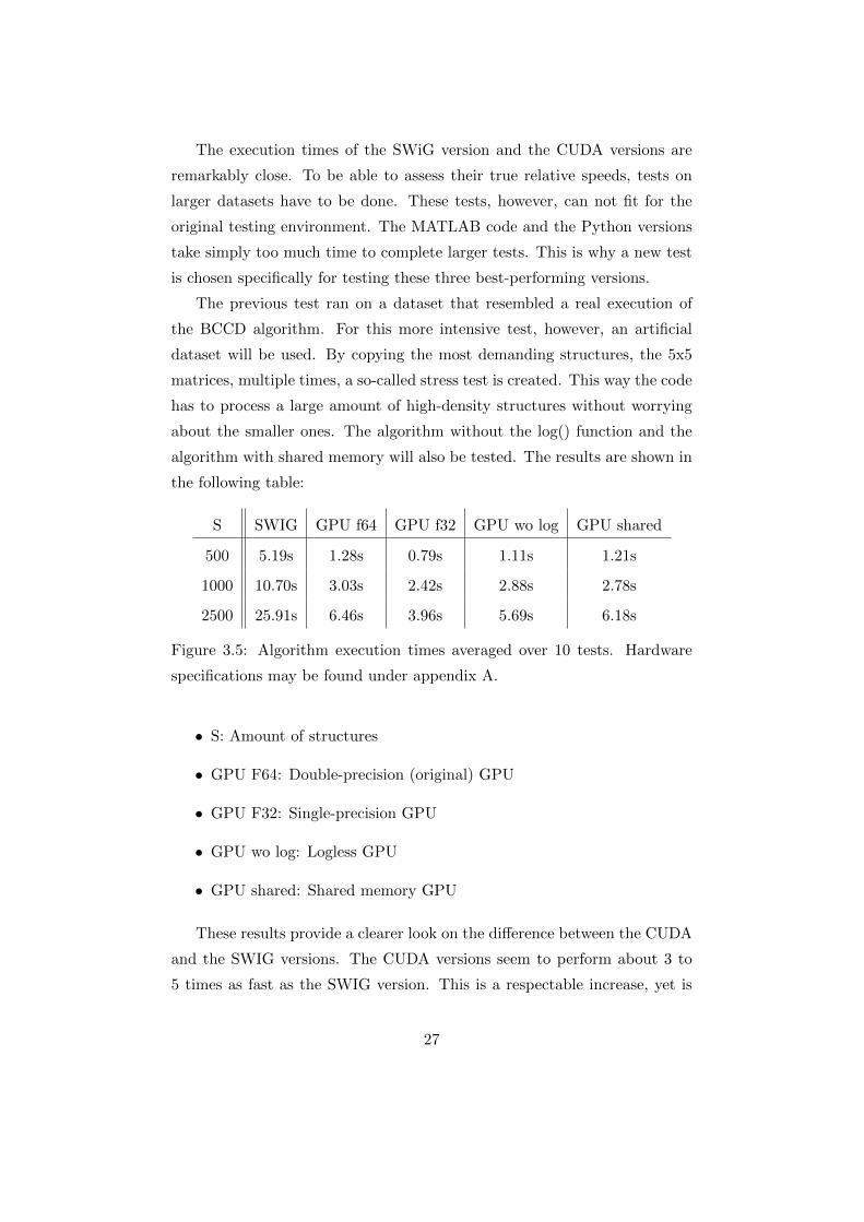
The execution times of the SWiG version and the CUDA versions are
remarkably close. To be able to assess their true relative speeds, tests on
larger datasets have to be done. These tests, however, can not fit for the
original testing environment. The MATLAB code and the Python versions
take simply too much time to complete larger tests. This is why a new test
is chosen specifically for testing these three best-performing versions.
The previous test ran on a dataset that resembled a real execution of
the BCCD algorithm. For this more intensive test, however, an artificial
dataset will be used. By copying the most demanding structures, the 5x5
matrices, multiple times, a so-called stress test is created. This way the code
has to process a large amount of high-density structures without worrying
about the smaller ones. The algorithm without the log() function and the
algorithm with shared memory will also be tested. The results are shown in
the following table:
S SWIG GPU f64 GPU f32 GPU wo log GPU shared
500 5.19s 1.28s 0.79s 1.11s 1.21s
1000 10.70s 3.03s 2.42s 2.88s 2.78s
2500 25.91s 6.46s 3.96s 5.69s 6.18s
Figure 3.5: Algorithm execution times averaged over 10 tests. Hardware
specifications may be found under appendix A.
• S: Amount of structures
• GPU F64: Double-precision (original) GPU
• GPU F32: Single-precision GPU
• GPU wo log: Logless GPU
• GPU shared: Shared memory GPU
These results provide a clearer look on the difference between the CUDA
and the SWIG versions. The CUDA versions seem to perform about 3 to
5 times as fast as the SWIG version. This is a respectable increase, yet is
27
not a massive boost in comparison to the difference between the MATLAB
version and the SWIG version. One possible explanation would be the still
somewhat limited parallelization. Even though the structures are being
scored in parallel, structures are subject to a maximum amount of loops.
This means that the amount of realized parallelization is still limited. A
possibility to enhance the speed would be to merge the scoring of multiple
structures into one kernel call. This would mean that the amount of loops
for a parallelization is vastly increased.
The single-precision version seems to take a larger lead in speed as the
problem becomes bigger. For the GPU, any double-precision operation is
split into four single-precision operations. This lead is thus expected. Both
the logless version and the shared memory version perform arguably better
than the original double-precision one. Even though the versions are faster,
the difference is almost negligible. The log() function does not seem to have
that much impact. Other memory optimizations may provide more usefull
that the use of shared memory.
28
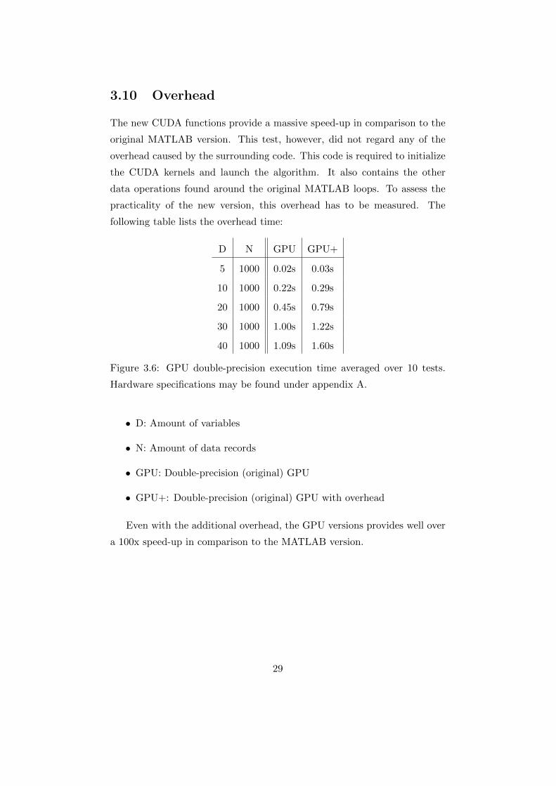
3.10 Overhead
The new CUDA functions provide a massive speed-up in comparison to the
original MATLAB version. This test, however, did not regard any of the
overhead caused by the surrounding code. This code is required to initialize
the CUDA kernels and launch the algorithm. It also contains the other
data operations found around the original MATLAB loops. To assess the
practicality of the new version, this overhead has to be measured. The
following table lists the overhead time:
D N GPU GPU+
5 1000 0.02s 0.03s
10 1000 0.22s 0.29s
20 1000 0.45s 0.79s
30 1000 1.00s 1.22s
40 1000 1.09s 1.60s
Figure 3.6: GPU double-precision execution time averaged over 10 tests.
Hardware specifications may be found under appendix A.
• D: Amount of variables
• N: Amount of data records
• GPU: Double-precision (original) GPU
• GPU+: Double-precision (original) GPU with overhead
Even with the additional overhead, the GPU versions provides well over
a 100x speed-up in comparison to the MATLAB version.
29
Chapter 4
Related Work
For this research, I have visited two summer schools (PRACE Maison de la
Simulation, PUMPS). Both were about the CUDA programming environ-
ment. On these summer schools, I have discussed my problem with fellow
students. I also got to enjoy their projects. The interesting thing about
these summer schools were that they drew applicants from all sort of fields.
The CUDA field has its fair share of host professional. CUDA, however,
is primarily also a tool to be used by different researcher to increase the
effectiveness of their code. This means that the people working with CUDA
use it for all kinds of applications. Attending the summer schools I did not
meet that many people utilizing CUDA for Machine Learning purposes. I,
however, did get to know a fair share about other CUDA implementations.
CUDA is an environment that is very powerful. It can be used to great
effect, but requires time to be implemented correctly. NVIDIA is slowly
making CUDA more mainstream by heavily promoting the studying of it.
Summer schools like I have attended provide a solid ground for students and
researchers to become familiar with the technology.
Machine learning is becoming more and more popular quickly.[5] The
combination of CUDA and Machine Learning is yet in its infancy.[1] The
medical sector proves to be an interesting vocal point for these developments.
[4] [6] Due to the popularity of Machine Learning, NVIDIA is currently
heavily promoting mixing the two.
30
Chapter 5
Conclusions
Even though the speed-up is massive for larger datasets, the current ap-
plicability is limited. All the new versions of the algorithm use Python to
load in the MATLAB workspace. This makes the current implementation
too impractical. First, the MATLAB script has to be run to export all the
workspace values. Afterwards, the values have to be read by the Python
script. The GPU accelerated algorithm can then use these values to cal-
culate the scores. These scores have to then be loaded into the MATLAB
workspace, creating even more overhead. Streamlining this process would
make the current code highly practical, yet has not been done yet due to
time constraints.
Even though there are still some practical challenges to overcome, it
has been proven that high-performance computing can serve as a solution
for the BCCD algorithm. By locating and rewriting the mayor bottleneck
in the code the BCCD algorithm has been increased in speed in a very
effective way. It seems, however, that there is still performance to be gained.
Most of the current performance gain is realized by more efficient, rewritten
functions and the usage of a lower-level language. Parallelization has shown
a fair contribution but can still be explored further, eventually creating the
optimal algorithm.
31
Bibliography
[1] Ron Bekkerman, Mikhail Bilenko, and John Langford. Scaling up ma-
chine learning: Parallel and distributed approaches. Cambridge Univer-
sity Press, 2011.
[2] Tom Claassen and Tom Heskes. A bayesian approach to constraint
based causal inference. arXiv preprint arXiv:1210.4866, 2012.
[3] Pierre Kestener. Introduction to gpu computing with cuda. PRACE,
2015.
[4] Igor Kononenko. Machine learning for medical diagnosis: history, state
of the art and perspective. Artificial Intelligence in medicine, 23(1):89–
109, 2001.
[5] Steve Lohr. The age of big data. New York Times, 11, 2012.
[6] Peter Lucas. Bayesian analysis, pattern analysis, and data mining in
health care. Current opinion in critical care, 10(5):399–403, 2004.
[7] John Nickolls and William J Dally. The gpu computing era. IEEE
micro, (2):56–69, 2010.
[8] John D Owens, Mike Houston, David Luebke, Simon Green, John E
Stone, and James C Phillips. Gpu computing. Proceedings of the IEEE,
96(5):879–899, 2008.
[9] Luis Enrique Sucar. Graphical causal models. In Probabilistic Graphical
Models, pages 237–246. Springer, 2015.
[10] Sarah Tariq. An introduction to gpu computing and cuda architecture.
NVIDIA Corporation, 2011.
32
Appendix A
Appendix
A.1 A: Hardware specifications
OS Name Microsoft Windows 10 Pro
Version 10.0.14393 Build 14393
Intel(R) Core(TM) i7-4710HQ CPU @ 2.50GHz, 4 Cores, 8 Logical Processors
Installed Physical Memory (RAM) 16.0 GB
Total Physical Memory 15.9 GB
Available Physical Memory 6.65 GB
Total Virtual Memory 18.8 GB
Available Virtual Memory 7.32 GB
=================================================================================
Device name: GeForce GTX 860M
---------------------------------------------------------------------------------
Attributes:
MAX_THREADS_PER_BLOCK:1024
MAX_BLOCK_DIM_X:1024
MAX_BLOCK_DIM_Y:1024
MAX_BLOCK_DIM_Z:64
MAX_GRID_DIM_X:2147483647
MAX_GRID_DIM_Y:65535
33
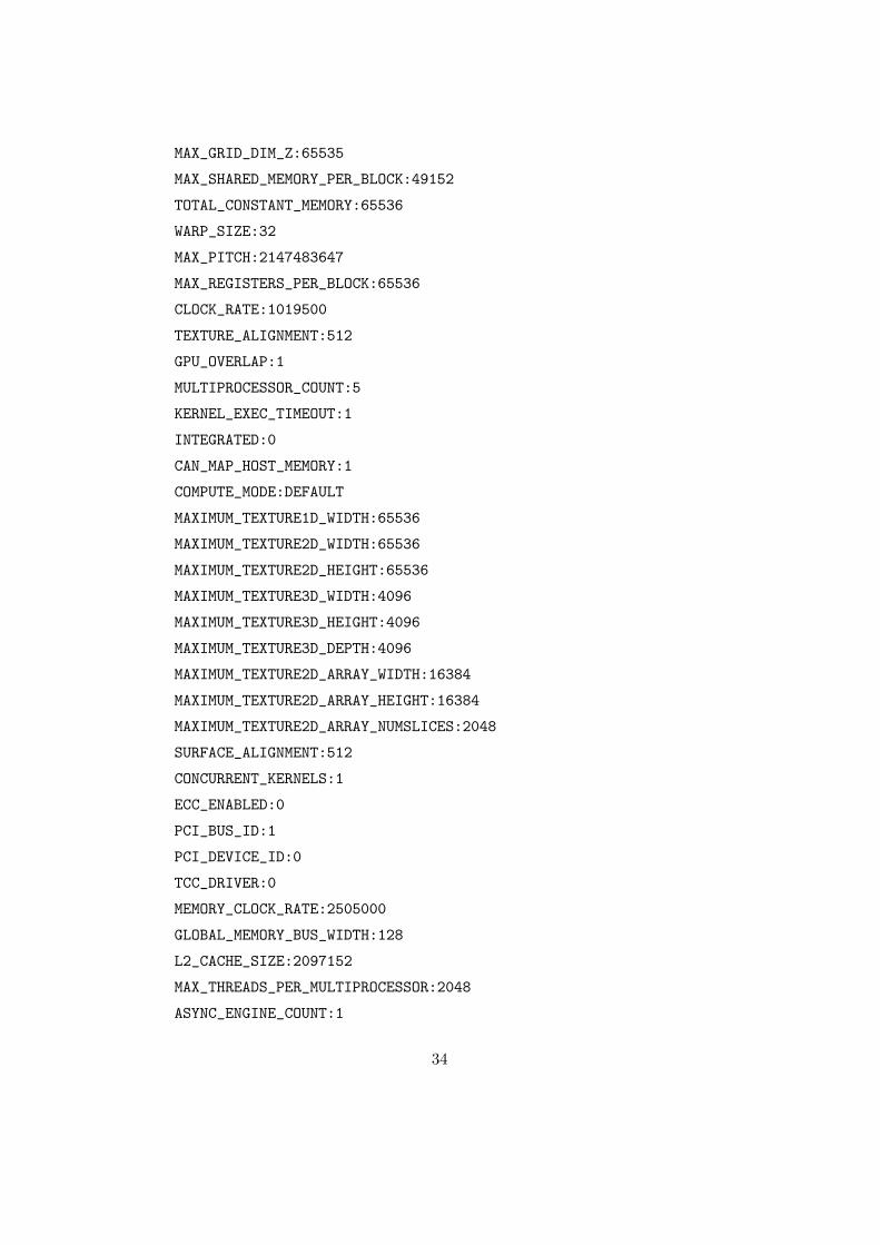
MAX_GRID_DIM_Z:65535
MAX_SHARED_MEMORY_PER_BLOCK:49152
TOTAL_CONSTANT_MEMORY:65536
WARP_SIZE:32
MAX_PITCH:2147483647
MAX_REGISTERS_PER_BLOCK:65536
CLOCK_RATE:1019500
TEXTURE_ALIGNMENT:512
GPU_OVERLAP:1
MULTIPROCESSOR_COUNT:5
KERNEL_EXEC_TIMEOUT:1
INTEGRATED:0
CAN_MAP_HOST_MEMORY:1
COMPUTE_MODE:DEFAULT
MAXIMUM_TEXTURE1D_WIDTH:65536
MAXIMUM_TEXTURE2D_WIDTH:65536
MAXIMUM_TEXTURE2D_HEIGHT:65536
MAXIMUM_TEXTURE3D_WIDTH:4096
MAXIMUM_TEXTURE3D_HEIGHT:4096
MAXIMUM_TEXTURE3D_DEPTH:4096
MAXIMUM_TEXTURE2D_ARRAY_WIDTH:16384
MAXIMUM_TEXTURE2D_ARRAY_HEIGHT:16384
MAXIMUM_TEXTURE2D_ARRAY_NUMSLICES:2048
SURFACE_ALIGNMENT:512
CONCURRENT_KERNELS:1
ECC_ENABLED:0
PCI_BUS_ID:1
PCI_DEVICE_ID:0
TCC_DRIVER:0
MEMORY_CLOCK_RATE:2505000
GLOBAL_MEMORY_BUS_WIDTH:128
L2_CACHE_SIZE:2097152
MAX_THREADS_PER_MULTIPROCESSOR:2048
ASYNC_ENGINE_COUNT:1
34
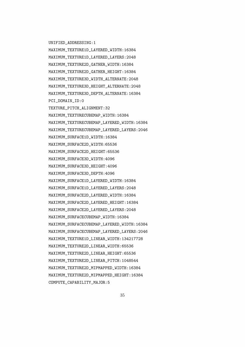
UNIFIED_ADDRESSING:1
MAXIMUM_TEXTURE1D_LAYERED_WIDTH:16384
MAXIMUM_TEXTURE1D_LAYERED_LAYERS:2048
MAXIMUM_TEXTURE2D_GATHER_WIDTH:16384
MAXIMUM_TEXTURE2D_GATHER_HEIGHT:16384
MAXIMUM_TEXTURE3D_WIDTH_ALTERNATE:2048
MAXIMUM_TEXTURE3D_HEIGHT_ALTERNATE:2048
MAXIMUM_TEXTURE3D_DEPTH_ALTERNATE:16384
PCI_DOMAIN_ID:0
TEXTURE_PITCH_ALIGNMENT:32
MAXIMUM_TEXTURECUBEMAP_WIDTH:16384
MAXIMUM_TEXTURECUBEMAP_LAYERED_WIDTH:16384
MAXIMUM_TEXTURECUBEMAP_LAYERED_LAYERS:2046
MAXIMUM_SURFACE1D_WIDTH:16384
MAXIMUM_SURFACE2D_WIDTH:65536
MAXIMUM_SURFACE2D_HEIGHT:65536
MAXIMUM_SURFACE3D_WIDTH:4096
MAXIMUM_SURFACE3D_HEIGHT:4096
MAXIMUM_SURFACE3D_DEPTH:4096
MAXIMUM_SURFACE1D_LAYERED_WIDTH:16384
MAXIMUM_SURFACE1D_LAYERED_LAYERS:2048
MAXIMUM_SURFACE2D_LAYERED_WIDTH:16384
MAXIMUM_SURFACE2D_LAYERED_HEIGHT:16384
MAXIMUM_SURFACE2D_LAYERED_LAYERS:2048
MAXIMUM_SURFACECUBEMAP_WIDTH:16384
MAXIMUM_SURFACECUBEMAP_LAYERED_WIDTH:16384
MAXIMUM_SURFACECUBEMAP_LAYERED_LAYERS:2046
MAXIMUM_TEXTURE1D_LINEAR_WIDTH:134217728
MAXIMUM_TEXTURE2D_LINEAR_WIDTH:65536
MAXIMUM_TEXTURE2D_LINEAR_HEIGHT:65536
MAXIMUM_TEXTURE2D_LINEAR_PITCH:1048544
MAXIMUM_TEXTURE2D_MIPMAPPED_WIDTH:16384
MAXIMUM_TEXTURE2D_MIPMAPPED_HEIGHT:16384
COMPUTE_CAPABILITY_MAJOR:5
35
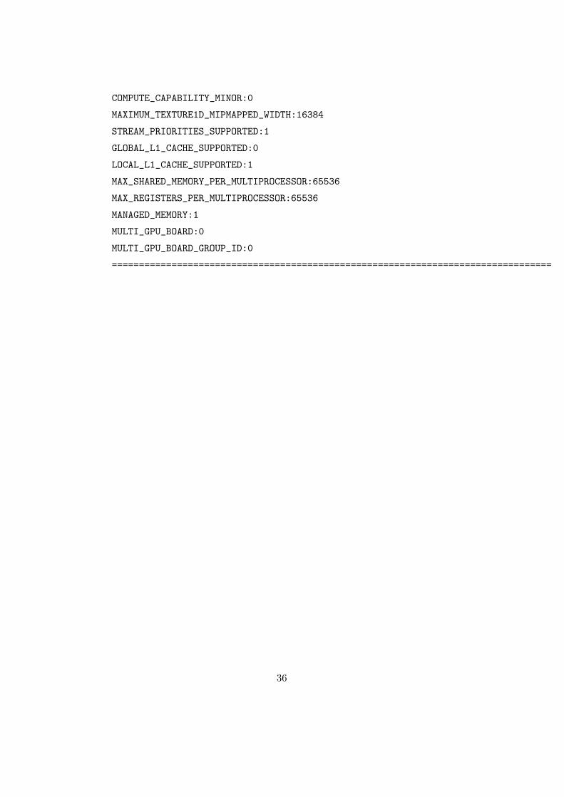
COMPUTE_CAPABILITY_MINOR:0
MAXIMUM_TEXTURE1D_MIPMAPPED_WIDTH:16384
STREAM_PRIORITIES_SUPPORTED:1
GLOBAL_L1_CACHE_SUPPORTED:0
LOCAL_L1_CACHE_SUPPORTED:1
MAX_SHARED_MEMORY_PER_MULTIPROCESSOR:65536
MAX_REGISTERS_PER_MULTIPROCESSOR:65536
MANAGED_MEMORY:1
MULTI_GPU_BOARD:0
MULTI_GPU_BOARD_GROUP_ID:0
=================================================================================
36
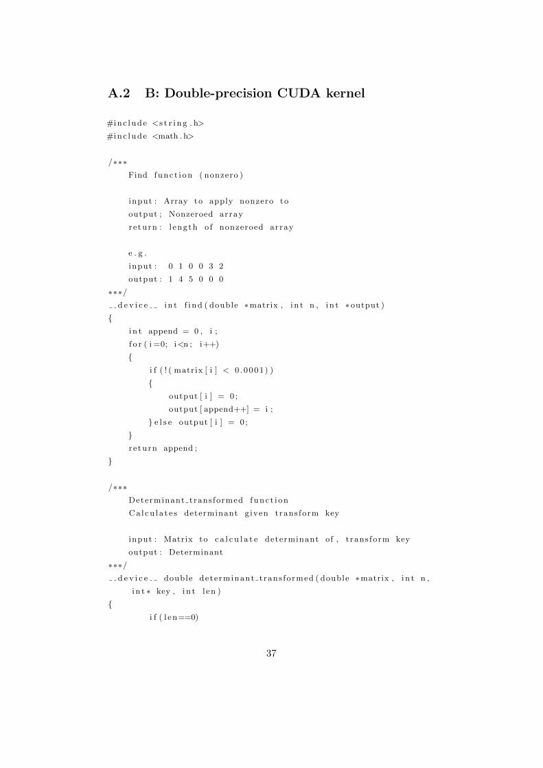
A.2 B: Double-precision CUDA kernel
#inc lude <s t r i n g . h>
#inc lude <math . h>
/∗∗∗Find func t i on ( nonzero )
input : Array to apply nonzero to
output ; Nonzeroed array
return : l ength o f nonzeroed array
e . g .
input : 0 1 0 0 3 2
output : 1 4 5 0 0 0
∗∗∗/d e v i c e i n t f i nd ( double ∗matrix , i n t n , i n t ∗output )
{i n t append = 0 , i ;
f o r ( i =0; i<n ; i++)
{i f ( ! ( matrix [ i ] < 0 .0001) )
{output [ i ] = 0 ;
output [ append++] = i ;
} e l s e output [ i ] = 0 ;
}re turn append ;
}
/∗∗∗Determinant transformed func t i on
Ca l cu l a t e s determinant g iven trans form key
input : Matrix to c a l c u l a t e determinant of , t rans form key
output : Determinant
∗∗∗/d e v i c e double determinant trans formed ( double ∗matrix , i n t n ,
i n t ∗ key , i n t l en )
{i f ( l en==0)
37
re turn
1 ;
i f ( l en==1)
return
matrix [ key [0 ]+n∗key [ 0 ] ] ;
i f ( l en==2)
return
matrix [ key [0 ]+n∗key [ 0 ] ] ∗ matrix [ key [1 ]+n∗key [ 1 ] ] −matrix [ key [1 ]+n∗key [ 0 ] ] ∗ matrix [ key [0 ]+n∗key [ 1 ] ] ;
i f ( l en==3)
return
matrix [ key [0 ]+n∗key [ 0 ] ] ∗ matrix [ key [1 ]+n∗key [ 1 ] ] ∗ matrix [ key
[2 ]+n∗key [ 2 ] ] +
matrix [ key [1 ]+n∗key [ 0 ] ] ∗ matrix [ key [2 ]+n∗key [ 1 ] ] ∗ matrix [ key
[0 ]+n∗key [ 2 ] ] +
matrix [ key [2 ]+n∗key [ 0 ] ] ∗ matrix [ key [0 ]+n∗key [ 1 ] ] ∗ matrix [ key
[1 ]+n∗key [ 2 ] ] −matrix [ key [2 ]+n∗key [ 0 ] ] ∗ matrix [ key [1 ]+n∗key [ 1 ] ] ∗ matrix [ key
[0 ]+n∗key [ 2 ] ] −matrix [ key [2 ]+n∗key [ 1 ] ] ∗ matrix [ key [1 ]+n∗key [ 2 ] ] ∗ matrix [ key
[0 ]+n∗key [ 0 ] ] −matrix [ key [2 ]+n∗key [ 2 ] ] ∗ matrix [ key [1 ]+n∗key [ 0 ] ] ∗ matrix [ key
[0 ]+n∗key [ 1 ] ] ;
i f ( l en==4)
return
matrix [ key [0 ]+n∗key [ 0 ] ] ∗ matrix [ key [1 ]+n∗key [ 1 ] ] ∗ matrix [ key
[2 ]+n∗key [ 2 ] ] ∗ matrix [ key [3 ]+n∗key [ 3 ] ] + . . . +
matrix [ key [3 ]+n∗key [ 0 ] ] ∗ matrix [ key [2 ]+n∗key [ 3 ] ] ∗ matrix [ key
[1 ]+n∗key [ 1 ] ] ∗ matrix [ key [0 ]+n∗key [ 2 ] ] ;
i f ( l en==5)
return
matrix [ key [0 ]+n∗key [ 0 ] ] ∗ matrix [ key [1 ]+n∗key [ 1 ] ] ∗ matrix [ key
[2 ]+n∗key [ 2 ] ] ∗ matrix [ key [3 ]+n∗key [ 3 ] ] ∗ matrix [ key [4 ]+n∗key[ 4 ] ] + . . . +
matrix [ key [4 ]+n∗key [ 0 ] ] ∗ matrix [ key [3 ]+n∗key [ 1 ] ] ∗ matrix [ key
[2 ]+n∗key [ 4 ] ] ∗ matrix [ key [1 ]+n∗key [ 2 ] ] ∗ matrix [ key [0 ]+n∗key[ 3 ] ] ;
r e turn 0 ;
}
38
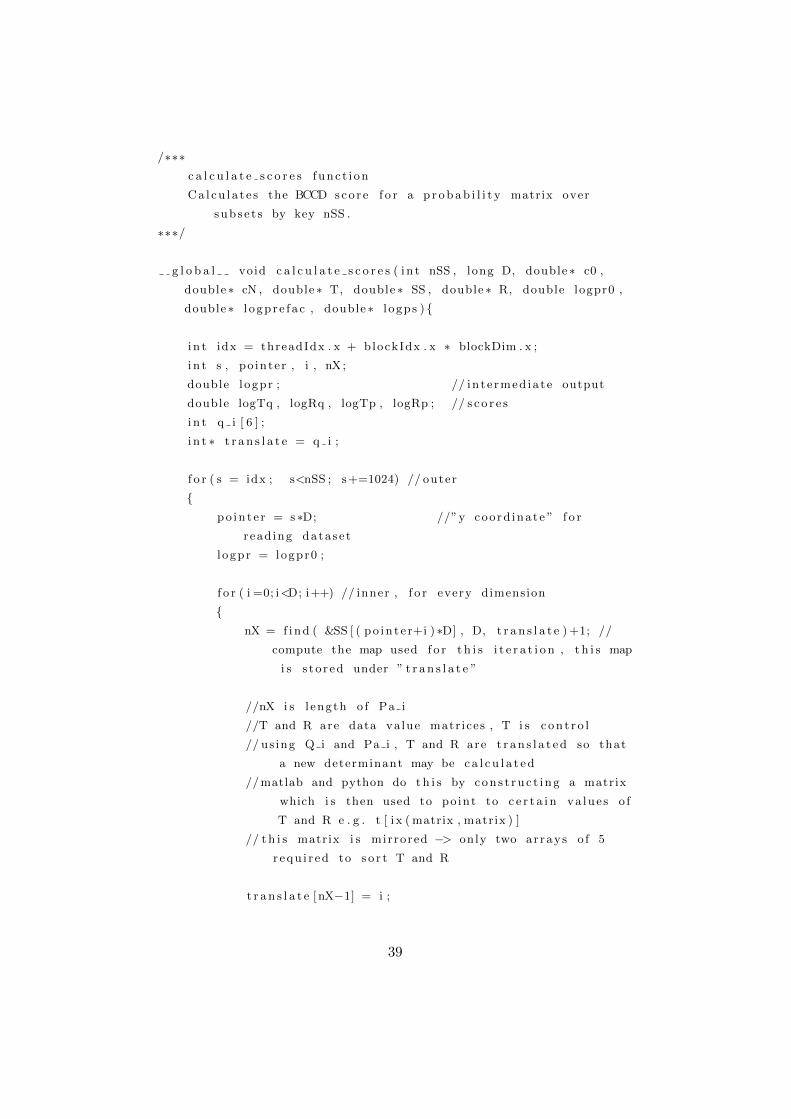
/∗∗∗c a l c u l a t e s c o r e s func t i on
Ca l cu l a t e s the BCCD sco r e f o r a p r obab i l i t y matrix over
subse t s by key nSS .
∗∗∗/
g l o b a l void c a l c u l a t e s c o r e s ( i n t nSS , long D, double ∗ c0 ,
double ∗ cN , double ∗ T, double ∗ SS , double ∗ R, double logpr0 ,
double ∗ l o gp r e f a c , double ∗ l ogps ) {
i n t idx = threadIdx . x + blockIdx . x ∗ blockDim . x ;
i n t s , po inter , i , nX;
double l ogpr ; // in te rmed ia t e output
double logTq , logRq , logTp , logRp ; // s c o r e s
i n t q i [ 6 ] ;
i n t ∗ t r a n s l a t e = q i ;
f o r ( s = idx ; s<nSS ; s+=1024) // outer
{po in t e r = s ∗D; //”y coord inate ” f o r
read ing datase t
l ogpr = logpr0 ;
f o r ( i =0; i<D; i++) // inner , f o r every dimension
{nX = f ind ( &SS [ ( po in t e r+i ) ∗D] , D, t r a n s l a t e )+1; //
compute the map used f o r t h i s i t e r a t i o n , t h i s map
i s s to r ed under ” t r a n s l a t e ”
//nX i s l ength o f Pa i
//T and R are data value matr ices , T i s c on t r o l
// us ing Q i and Pa i , T and R are t r an s l a t ed so that
a new determinant may be c a l c u l a t ed
//matlab and python do t h i s by con s t ru c t i ng a matrix
which i s then used to po int to c e r t a i n va lue s o f
T and R e . g . t [ i x ( matrix , matrix ) ]
// t h i s matrix i s mirrored −> only two ar rays o f 5
r equ i r ed to s o r t T and R
t r a n s l a t e [nX−1] = i ;
39
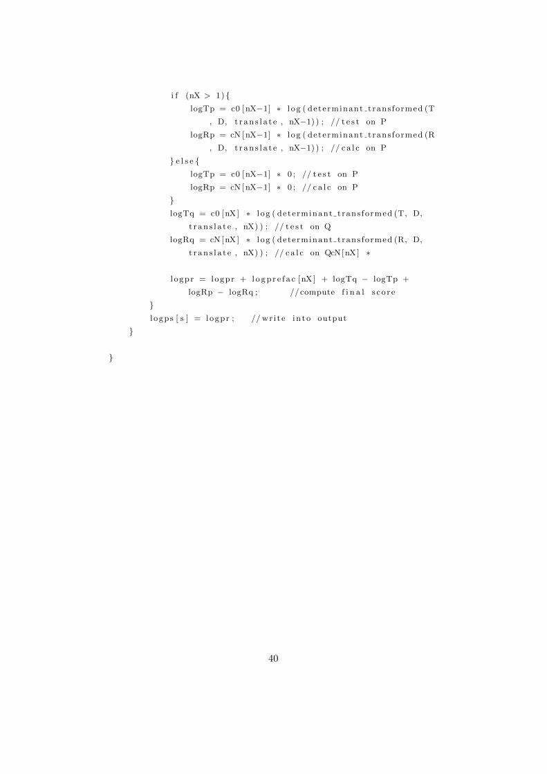
i f (nX > 1) {logTp = c0 [nX−1] ∗ l og ( determinant trans formed (T
, D, t r an s l a t e , nX−1) ) ; // t e s t on P
logRp = cN [nX−1] ∗ l og ( determinant trans formed (R
, D, t r an s l a t e , nX−1) ) ; // c a l c on P
} e l s e {logTp = c0 [nX−1] ∗ 0 ; // t e s t on P
logRp = cN [nX−1] ∗ 0 ; // c a l c on P
}logTq = c0 [nX] ∗ l og ( determinant trans formed (T, D,
t r an s l a t e , nX) ) ; // t e s t on Q
logRq = cN [nX] ∗ l og ( determinant trans formed (R, D,
t r an s l a t e , nX) ) ; // c a l c on QcN[nX] ∗
l ogpr = logpr + l o gp r e f a c [nX] + logTq − logTp +
logRp − logRq ; //compute f i n a l s c o r e
}l ogps [ s ] = logpr ; // wr i t e in to output
}
}
40