Accelerated Training of Max-Margin Markov Networks with

Kernels

Xinhua Zhang∗

Department of Computing Science, University of Alberta, Edmonton, AB T6G2E8, Canada

Ankan Saha

Department of Computer Science, University of Chicago, Chicago, IL 60637, USA

S.V.N. Vishwanathan

Department of Statistics and Computer Science, Purdue University, West Lafayette, IN 47907, USA

Abstract

Structured output prediction is an important machine learning problem both in theory

and practice, and the max-margin Markov network (M3N) is an effective approach. All

state-of-the-art algorithms for optimizing M3N objectives take at least O(1/ε) number of

iterations to find an ε accurate solution. Nesterov [1] broke this barrier by proposing an

excessive gap reduction technique (EGR) which converges in O(1/√ε) iterations. However,

it is restricted to Euclidean projections which consequently requires an intractable amount

of computation for each iteration when applied to solve M3N. In this paper, we show that by

extending EGR to Bregman projection, this faster rate of convergence can be retained, and

more importantly, the updates can be performed efficiently by exploiting graphical model

factorization. Further, we design a kernelized procedure which allows all computations per

iteration to be performed at the same cost as the state-of-the-art approaches.

Keywords: Convex optimization, max-margin models, kernel method, graphical models

∗Corresponding authorEmail addresses: xinhua2@cs.ualberta.ca (Xinhua Zhang), ankans@cs.uchicago.edu (Ankan

Saha), vishy@stat.purdue.edu (S.V.N. Vishwanathan)

Preprint submitted to Theoretical Computer Science February 26, 2013

1. Introduction

In the supervised learning setting, one is given a training set of labeled data points and

the aim is to learn a function which predicts labels on unseen data points. Sometimes the

label space has a rich internal structure which characterizes the combinatorial or recursive

inter-dependencies of the application domain. It is widely believed that capturing these

dependencies is critical for effectively learning with structured output. Examples of such

problems include sequence labeling, context free grammar parsing, and word alignment.

However, parameter estimation is generally hard even for simple linear models, because the

size of the label space is potentially exponentially large (see e.g. [2]). Therefore it is crucial to

exploit the underlying conditional independence assumptions for the sake of computational

tractability. This is often done by defining a graphical model on the output space, and

exploiting the underlying graphical model factorization to perform efficient computations.

Research in structured prediction can broadly be categorized into two tracks: Optimizing

conditional likelihood in an exponential family results in conditional random fields [CRFs,

3], and a maximum margin approach leads to max-margin Markov networks [M3Ns, 4].

Unsurprisingly, these two approaches share many commonalities: First, they both minimize

a regularized risk with a square norm regularizer. Second, they assume that there is a

joint feature map φ which maps (x,y) to a feature vector in Rp.1 Third, they assume a

label loss `(y,yi; xi) which quantifies the loss of predicting label y when the correct label of

input xi is yi. Finally, they assume that the space of labels Y is endowed with a graphical

model structure and that φ(x,y) and `(y,yi; xi) factorize according to the cliques of this

graphical model. The main difference is in the loss function employed. CRFs minimize the

L2-regularized logistic loss:

J(w) =λ

2‖w‖2

2 +1

n

n∑i=1

log∑y∈Y

exp(`(y,yi; xi)−

⟨w,φ(xi,yi)− φ(xi,y)

⟩), (1)

1We discuss kernels and associated feature maps into a Reproducing Kernel Hilbert Space (RKHS) in

Section 4.3.

2

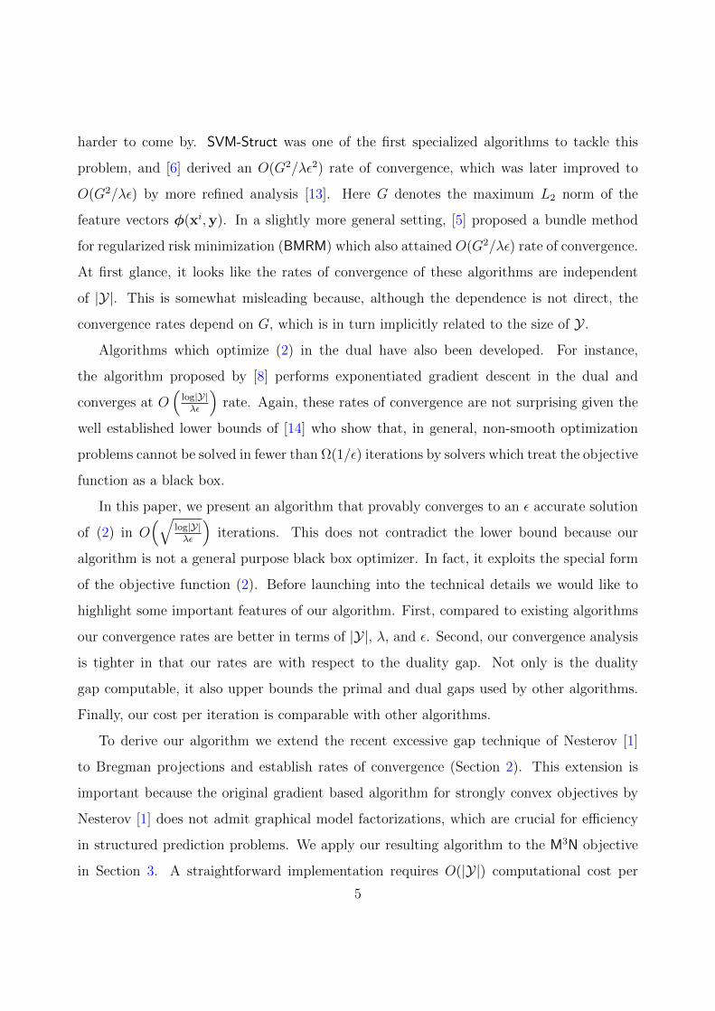
dual gap

duality gap

primal gap

used by [7]

and ours

used by [8] and

[9, Chapter 6]

(a) Primal gap, dual gap, and duality gap

primal gap

Gap used by

BMRM in [5]

(b) BMRM gap (and similarly for SVM-Struct)

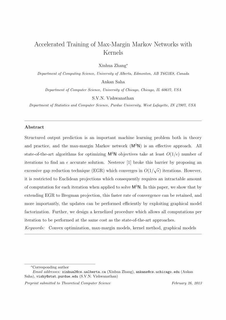
Figure 1: Illustration of stopping criterion monitored by various algorithms; convergence rates are stated

with respect to these stopping criterion. D(α) is the Lagrange dual of J(w), and minw J(w) = maxαD(α).

Neither the primal gap nor the dual gap is actually measurable in practice since minw J(w) (and maxαD(α))

is unknown. BMRM (right) therefore uses a measurable upper bound of the primal gap. SVM-Struct monitors

constraint violation, which can be also be translated to an upper bound on the primal gap.

where all log in this paper stands for natural basis. In contrast, the M3Ns minimize the

L2-regularized hinge loss

J(w) =λ

2‖w‖2

2 +1

n

n∑i=1

maxy∈Y

`(y,yi; xi)−

⟨w,φ(xi,yi)− φ(xi,y)

⟩. (2)

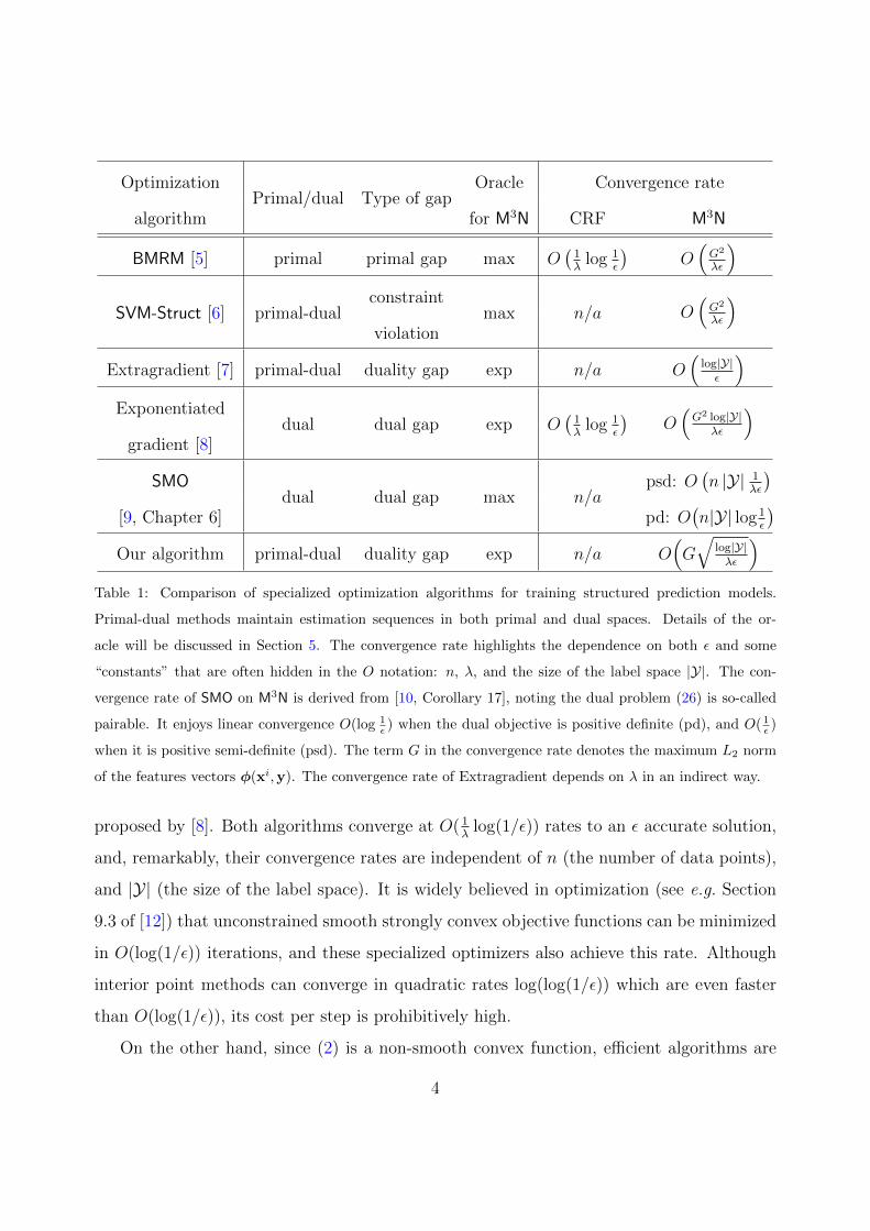
A large body of literature exists on efficient algorithms for minimizing the above objective

functions. A summary of existing methods, and their convergence rates (iterations needed

to find an ε accurate solution) can be found in Table 1. The ε accuracy of a solution can be

measured in many different ways and different algorithms employ different but somewhat

related stopping criterion (see Figure 1). Some produce iterates wk in the primal space and

bound the primal gap J(wk)−minw J(w). Some solve the dual problem D(α) with iterates

αk and bound the dual gap maxαD(α) − D(αk). Some bound the duality gap J(wk) −

D(αk), and still others bound J(wk)−minw Jk(w) where Jk is a uniform lower bound of J .

This must be borne in mind when interpreting the convergence rates in Table 1.

Since (1) is a smooth convex objective, classical methods such as L-BFGS can directly

be applied [11]. Specialized solvers also exist. For instance a primal algorithm based on

bundle methods was proposed by [5], while a dual algorithm for the same problem was

3

OptimizationPrimal/dual Type of gap

Oracle Convergence rate

algorithm for M3N CRF M3N

BMRM [5] primal primal gap max O(

1λ

log 1ε

)O(G2

λε

)SVM-Struct [6] primal-dual

constraintmax n/a O

(G2

λε

)violation

Extragradient [7] primal-dual duality gap exp n/a O(

log|Y|ε

)Exponentiated

dual dual gap exp O(

1λ

log 1ε

)O(G2 log|Y|

λε

)gradient [8]

SMOdual dual gap max n/a

psd: O(n |Y| 1

λε

)[9, Chapter 6] pd: O

(n|Y| log 1

ε

)Our algorithm primal-dual duality gap exp n/a O

(G√

log|Y|λε

)Table 1: Comparison of specialized optimization algorithms for training structured prediction models.

Primal-dual methods maintain estimation sequences in both primal and dual spaces. Details of the or-

acle will be discussed in Section 5. The convergence rate highlights the dependence on both ε and some

“constants” that are often hidden in the O notation: n, λ, and the size of the label space |Y|. The con-

vergence rate of SMO on M3N is derived from [10, Corollary 17], noting the dual problem (26) is so-called

pairable. It enjoys linear convergence O(log 1ε ) when the dual objective is positive definite (pd), and O( 1

ε )

when it is positive semi-definite (psd). The term G in the convergence rate denotes the maximum L2 norm

of the features vectors φ(xi,y). The convergence rate of Extragradient depends on λ in an indirect way.

proposed by [8]. Both algorithms converge at O( 1λ

log(1/ε)) rates to an ε accurate solution,

and, remarkably, their convergence rates are independent of n (the number of data points),

and |Y| (the size of the label space). It is widely believed in optimization (see e.g. Section

9.3 of [12]) that unconstrained smooth strongly convex objective functions can be minimized

in O(log(1/ε)) iterations, and these specialized optimizers also achieve this rate. Although

interior point methods can converge in quadratic rates log(log(1/ε)) which are even faster

than O(log(1/ε)), its cost per step is prohibitively high.

On the other hand, since (2) is a non-smooth convex function, efficient algorithms are

4

harder to come by. SVM-Struct was one of the first specialized algorithms to tackle this

problem, and [6] derived an O(G2/λε2) rate of convergence, which was later improved to

O(G2/λε) by more refined analysis [13]. Here G denotes the maximum L2 norm of the

feature vectors φ(xi,y). In a slightly more general setting, [5] proposed a bundle method

for regularized risk minimization (BMRM) which also attained O(G2/λε) rate of convergence.

At first glance, it looks like the rates of convergence of these algorithms are independent

of |Y|. This is somewhat misleading because, although the dependence is not direct, the

convergence rates depend on G, which is in turn implicitly related to the size of Y .

Algorithms which optimize (2) in the dual have also been developed. For instance,

the algorithm proposed by [8] performs exponentiated gradient descent in the dual and

converges at O(

log|Y|λε

)rate. Again, these rates of convergence are not surprising given the

well established lower bounds of [14] who show that, in general, non-smooth optimization

problems cannot be solved in fewer than Ω(1/ε) iterations by solvers which treat the objective

function as a black box.

In this paper, we present an algorithm that provably converges to an ε accurate solution

of (2) in O(√

log|Y|λε

)iterations. This does not contradict the lower bound because our

algorithm is not a general purpose black box optimizer. In fact, it exploits the special form

of the objective function (2). Before launching into the technical details we would like to

highlight some important features of our algorithm. First, compared to existing algorithms

our convergence rates are better in terms of |Y|, λ, and ε. Second, our convergence analysis

is tighter in that our rates are with respect to the duality gap. Not only is the duality

gap computable, it also upper bounds the primal and dual gaps used by other algorithms.

Finally, our cost per iteration is comparable with other algorithms.

To derive our algorithm we extend the recent excessive gap technique of Nesterov [1]

to Bregman projections and establish rates of convergence (Section 2). This extension is

important because the original gradient based algorithm for strongly convex objectives by

Nesterov [1] does not admit graphical model factorizations, which are crucial for efficiency

in structured prediction problems. We apply our resulting algorithm to the M3N objective

in Section 3. A straightforward implementation requires O(|Y|) computational cost per

5

iteration, which makes it prohibitively expensive. We show that by exploiting the graphical

model structure of Y the cost per iteration can be reduced to O(log |Y|) (Section 4). Finally

we contrast our algorithm with existing techniques in Section 5.

2. Excessive Gap Technique with Bregman Projection

The excessive gap technique proposed by Nesterov [1] achieves accelerated rate of conver-

gence only when the Euclidean projection is used. This prevents the algorithm from being

applied to train M3N efficiently, and the aim of this section is to extend the approach to

Bregman projection. We start by recapping the algorithm.

The following three concepts from convex analysis will be extensively used in the sequel.

Define R := R ∪ ∞. For any convex function f , its domain is defined as the set of x

where f(x) is not infinity: dom f = x : f(x) <∞. Denote its continuous domain as

contf = x ∈ dom f : f is continuous at x. The dual norm of a norm ‖·‖ is denoted as

‖·‖∗.

Definition 1. A convex function f : Rn → R is strongly convex with respect to a norm

‖ · ‖ if there exists a constant ρ > 0 such that f − ρ2‖ · ‖2 is convex. The maximum of such

constants, ρ∗ is called the modulus of strong convexity of f , and for brevity we will call f

ρ∗-strongly convex.

Definition 2. Suppose a function f : Rn → R is differentiable on Q ⊆ Rn. Then f is said

to have Lipschitz continuous gradient (l.c.g) with respect to a norm ‖ · ‖ if there exists a

constant L such that

‖∇f(w)−∇f(w′)‖∗ ≤ L‖w −w′‖ ∀ w,w′ ∈ Q. (3)

For brevity, we will call f L-l.c.g.

An important consequence of l.c.g is to upper bound a convex function by a quadratic.

Lemma 1 ([15, Eq 3.1]). A convex function f is L-l.c.g if, and only if, it is differentiable

everywhere in its domain and

f(w′) ≤ f(w) + 〈∇f(w),w′ −w〉+L

2‖w′ −w‖2

, ∀ w,w′ ∈ dom f.

6

Definition 3. The Fenchel dual of a function f : Rn → R is a function f ? : Rn → R defined

by

f ?(w?) = supw∈Rn

〈w,w?〉 − f(w) . (4)

The definition of Fenchel duality gives a convenient characterization of the gradient of

f ?.

Lemma 2 ([16, Corollary X.1.4.4]). If f ? is differentiable at w?, then

∇f ?(w?) = argsupw∈Rn

〈w,w?〉 − f(w) ,

and the argsup must be attainable and unique. Thus argsup can be replaced by argmax.

Strong convexity and l.c.g are related by Fenchel duality according to the following

lemma:

Lemma 3 ([16, Theorem 4.2.1 and 4.2.2]).

1. If f : Rn → R is ρ-strongly convex, then f ? is finite on Rn and f ? is differentiable and

1ρ-l.c.g.

2. If f : Rn → R is convex on Rn and L-l.c.g, then f ? is 1L

-strongly convex.

Let Q1 and Q2 be subsets of Euclidean spaces and A be a linear map from Q1 to Q2.

Suppose f and g are convex functions defined on Q1 and Q2 respectively. We are interested

in the following optimization problem:

minw∈Q1

J(w)

where J(w) := f(w) + g?(Aw) = f(w) + maxα∈Q2

〈Aw,α〉 − g(α) . (5)

We will make the following standard assumptions: a) Q2 is compact; b) with respect to

a certain norm on Q1, the function f defined on Q1 is ρ-strongly convex (ρ > 0) but not

necessarily l.c.g , and c) with respect to a certain norm on Q2 (which can be different from

that on Q1), the function g defined on Q2 is Lg-l.c.g and convex, but not necessarily strongly

7

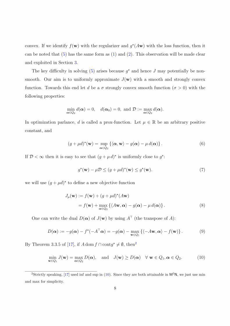
convex. If we identify f(w) with the regularizer and g?(Aw) with the loss function, then it

can be noted that (5) has the same form as (1) and (2). This observation will be made clear

and exploited in Section 3.

The key difficulty in solving (5) arises because g? and hence J may potentially be non-

smooth. Our aim is to uniformly approximate J(w) with a smooth and strongly convex

function. Towards this end let d be a σ strongly convex smooth function (σ > 0) with the

following properties:

minα∈Q2

d(α) = 0, d(α0) = 0, and D := maxα∈Q2

d(α).

In optimization parlance, d is called a prox-function. Let µ ∈ R be an arbitrary positive

constant, and

(g + µd)?(w) = supα∈Q2

〈α,w〉 − g(α)− µ d(α) . (6)

If D <∞ then it is easy to see that (g + µ d)? is uniformly close to g?:

g?(w)− µD ≤ (g + µd)?(w) ≤ g?(w). (7)

we will use (g + µd)? to define a new objective function

Jµ(w) := f(w) + (g + µd)?(Aw)

= f(w) + maxα∈Q2

〈Aw,α〉 − g(α)− µ d(α) . (8)

One can write the dual D(α) of J(w) by using A> (the transpose of A):

D(α) := −g(α)− f ?(−A>α) = −g(α)− maxw∈Q1

〈−Aw,α〉 − f(w) . (9)

By Theorem 3.3.5 of [17], if A dom f ∩ contg? 6= ∅, then2

minw∈Q1

J(w) = maxα∈Q2

D(α), and J(w) ≥ D(α) ∀ w ∈ Q1,α ∈ Q2. (10)

2Strictly speaking, [17] used inf and sup in (10). Since they are both attainable in M3N, we just use min

and max for simplicity.

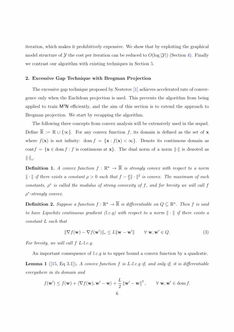
8

J(w)

D(α)

J(w)

D(α)

Jµk(w)µkD

J(w)

D(α)

Jµk(w)µkD

Jµk(wk)

D(αk)

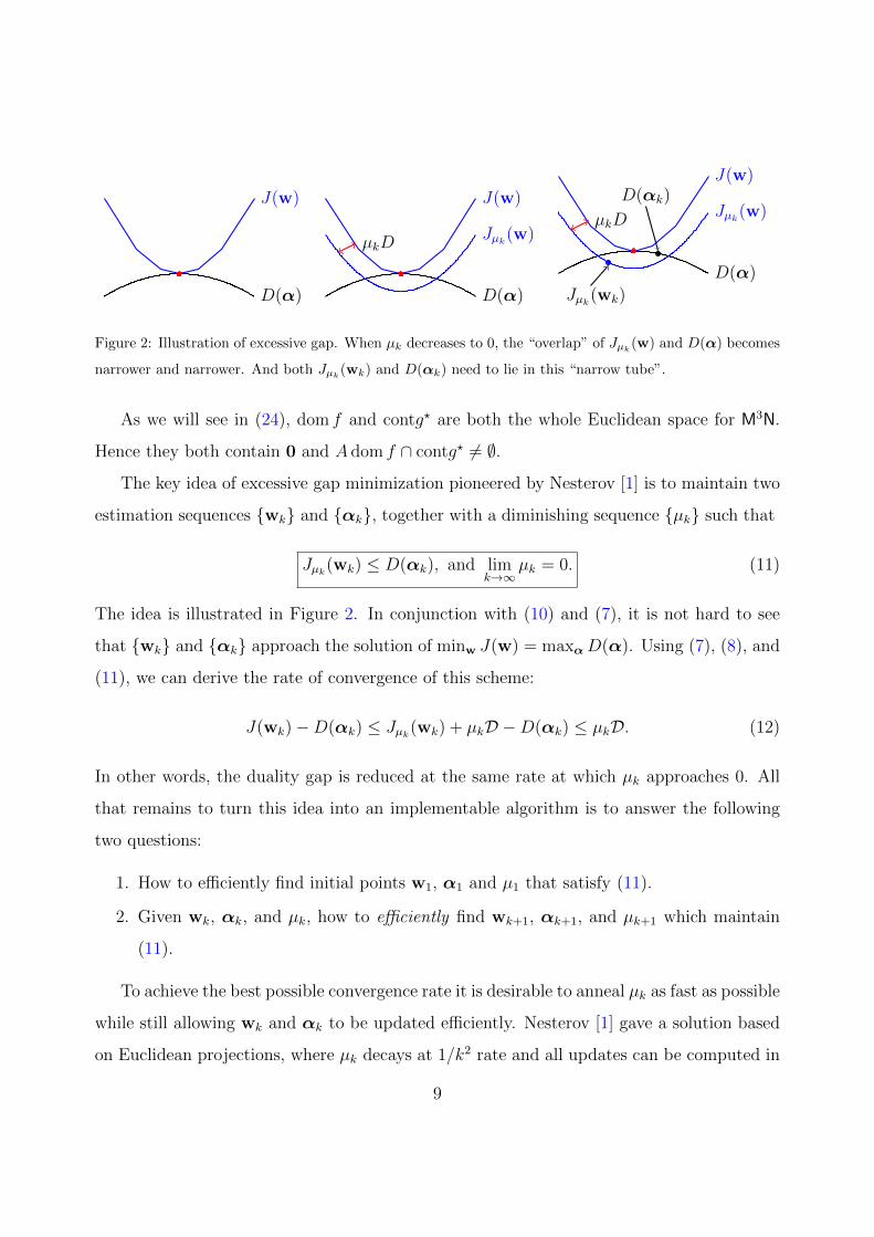
Figure 2: Illustration of excessive gap. When µk decreases to 0, the “overlap” of Jµk(w) and D(α) becomes

narrower and narrower. And both Jµk(wk) and D(αk) need to lie in this “narrow tube”.

As we will see in (24), dom f and contg? are both the whole Euclidean space for M3N.

Hence they both contain 0 and A dom f ∩ contg? 6= ∅.

The key idea of excessive gap minimization pioneered by Nesterov [1] is to maintain two

estimation sequences wk and αk, together with a diminishing sequence µk such that

Jµk(wk) ≤ D(αk), and limk→∞

µk = 0. (11)

The idea is illustrated in Figure 2. In conjunction with (10) and (7), it is not hard to see

that wk and αk approach the solution of minw J(w) = maxαD(α). Using (7), (8), and

(11), we can derive the rate of convergence of this scheme:

J(wk)−D(αk) ≤ Jµk(wk) + µkD −D(αk) ≤ µkD. (12)

In other words, the duality gap is reduced at the same rate at which µk approaches 0. All

that remains to turn this idea into an implementable algorithm is to answer the following

two questions:

1. How to efficiently find initial points w1, α1 and µ1 that satisfy (11).

2. Given wk, αk, and µk, how to efficiently find wk+1, αk+1, and µk+1 which maintain

(11).

To achieve the best possible convergence rate it is desirable to anneal µk as fast as possible

while still allowing wk and αk to be updated efficiently. Nesterov [1] gave a solution based

on Euclidean projections, where µk decays at 1/k2 rate and all updates can be computed in

9

closed form. We now extend his ideas to updates based on Bregman projections3, which will

be the key to our application to structured prediction problems later. Since d is differentiable,

we can define a Bregman divergence based on it:4

∆(α,α) := d(α)− d(α)− 〈∇d(α), α−α〉 . (13)

Given a point α and a direction g, we can define the Bregman projection as:

V (α,g) := argminα∈Q2

∆(α,α)+〈g, α−α〉 = argminα∈Q2

d(α)−〈∇d(α)−g, α〉.

For notational convenience, we define the following two maps:

w(α) := argmaxw∈Q1

〈−Aw,α〉 − f(w) = ∇f ?(−A>α) (14a)

αµ(w) := argmaxα∈Q2

〈Aw,α〉 − g(α)− µd(α) = ∇(g + µd)?(Aw), (14b)

where the last step of both (14a) and (14b) are due to Lemma 2. It should be noted that

αµk is a different sequence from the sequence of dual variables αk used in Algorithm 1 and

the two should not be confused. Here ∇f ?(−A>α) and ∇(g + µd)?(Aw) stand for the the

gradient of f ? evaluated at −A>α, and the gradient of (g + µd)? evaluated at Aw. Since

both f and g + µd are strongly convex, the above maps are unique and well defined. By

Lemma 2,

∇D(α) = −∇g(α) + Aw(α). (15)

Since f is assumed to be ρ-strongly convex, it follows from Lemma 3 that −D(α) is l.c.g .

If we denote its l.c.g modulus as L, then an easy calculation [e.g. Eq. (7.2) 1] shows that

L =1

ρ‖A‖2 + Lg, and ‖A‖ := max

‖w‖=‖α‖=1〈Aw,α〉 . (16)

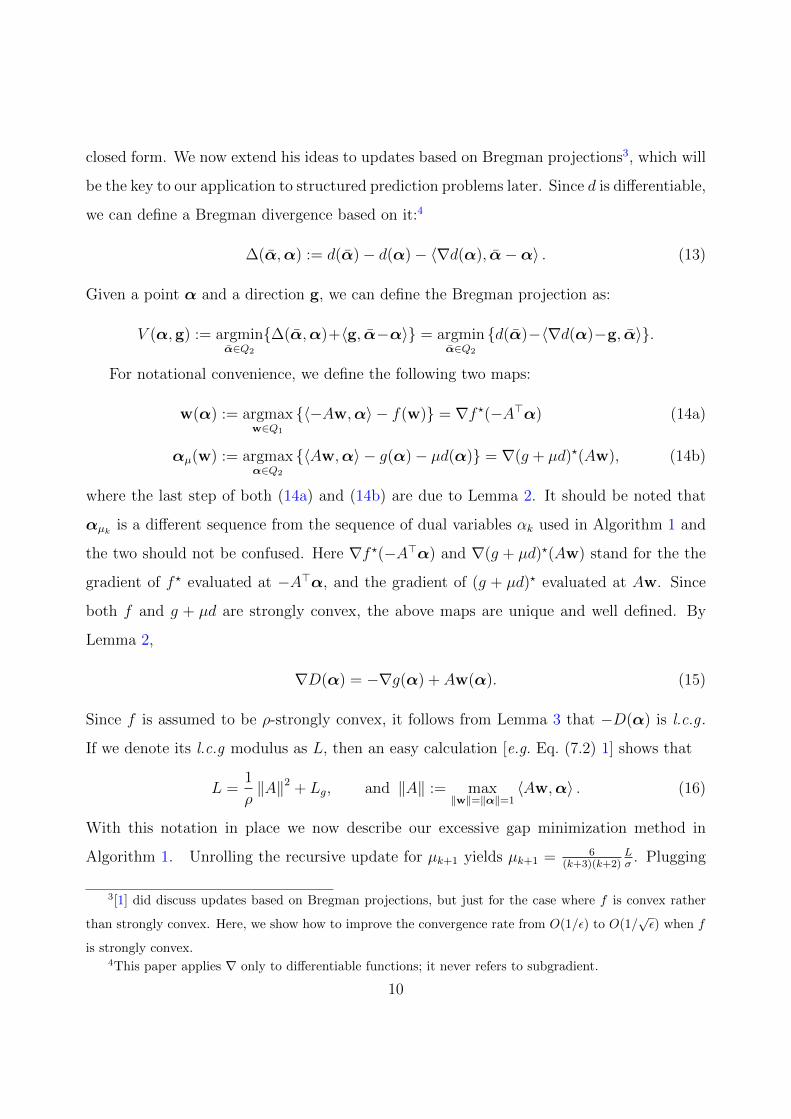
With this notation in place we now describe our excessive gap minimization method in

Algorithm 1. Unrolling the recursive update for µk+1 yields µk+1 = 6(k+3)(k+2)

Lσ

. Plugging

3[1] did discuss updates based on Bregman projections, but just for the case where f is convex rather

than strongly convex. Here, we show how to improve the convergence rate from O(1/ε) to O(1/√ε) when f

is strongly convex.4This paper applies ∇ only to differentiable functions; it never refers to subgradient.

10

Algorithm 1: Excessive gap minimization

Input: Function f which is strongly convex, convex function g which is l.c.g .

Output: Sequences wk, αk, and µk that satisfy (11), with limk→∞

µk = 0.

1 Initialize: α0 ← argminu∈Q2d(u), µ1 ← L

σ, w1 ← w(α0), α1 ← V

(α0,

−1µ1∇D(α0)

).

2 for k = 1, 2, . . . do

3 τk ← 2k+3

.

4 α← (1− τk)αk + τkαµk(wk).

5 wk+1 ← (1− τk)wk + τkw(α).

6 α← V(αµk(wk),

−τk(1−τk)µk

∇D(α))

.

7 αk+1 ← (1− τk)αk + τkα.

8 µk+1 ← (1− τk)µk.

this into (12) and using (16) immediately yields a O(1/√ε) rate of convergence of our

algorithm.

Theorem 4 (Rate of convergence for duality gap). The sequences wk and αk in Algo-

rithm 1 satisfy

J(wk)−D(αk) ≤6LD

σ(k + 1)(k + 2)=

6Dσ(k + 1)(k + 2)

(1

ρ‖A‖2 + Lg

). (17)

All that remains is to show that

Theorem 5. The updates in Algorithm 1 guarantee (11) is satisfied for all k ≥ 1.

To prove Theorem 5, we begin with a technical lemma.

Lemma 6. (Lemma 7.2 of [1]) For any α and α, we have

D(α) + 〈∇D(α), α−α〉 ≥ −g(α) + 〈Aw(α), α〉+ f(w(α)).

Proof. By directly applying (15) and using the fact that a convex function is always above

its first order Taylor approximation [16, Corollary 2.1.4], we obtain

D(α) + 〈∇D(α), α−α〉 = −g(α) + 〈Aw(α),α〉+ f(w(α)) + 〈−∇g(α) + Aw(α), α−α〉

≥ −g(α) + 〈Aw(α), α〉+ f(w(α)).

11

Furthermore, because d is σ-strongly convex, it follows that

∆(α,α) = d(α)− d(α)− 〈∇d(α), α−α〉 ≥ σ

2‖α−α‖2 . (18)

As α0 minimizes d over Q2, we have

〈∇d(α0),α−α0〉 ≥ 0 ∀ α ∈ Q2. (19)

Proof. (of Theorem 5) We first show that the initial w1 and α1 satisfy the excessive gap

condition (11). Since −D is L-l.c.g , so by Lemma 1

D(α1) ≥ D(α0) + 〈∇D(α0),α1 −α0〉 −1

2L ‖α1 −α0‖2

(by defn. of µ1 and (18)) ≥ D(α0) + 〈∇D(α0),α1 −α0〉 − µ1∆(α1,α0)

(by defn. of α1) = D(α0)− µ1 minα∈Q2

− µ−1

1 〈∇D(α0),α−α0〉+ ∆(α,α0)

(by (19) and d(α0) = 0) ≥ D(α0)−µ1 minα∈Q2

−µ−1

1 〈∇D(α0),α−α0〉+d(α)

= maxα∈Q2

D(α0) + 〈∇D(α0),α−α0〉 − µ1 d(α)

(by Lemma 6) ≥ maxα∈Q2

−g(α)+〈Aw(α0),α〉+f(w(α0))−µ1 d(α)

= Jµ1(w1),

which shows that our initialization indeed satisfies (11).

Second, we prove by induction that the updates in Algorithm 1 maintain (11). We begin

with two useful observations. Using µk+1 = 6(k+3)(k+2)

Lσ

and the definition of τk, one can

bound

µk+1 =6

(k + 3)(k + 2)

L

σ≥ τ 2

k

L

σ. (20)

Let β := αµk(wk). The optimality conditions for (14b) imply

〈µk∇d(β)− Awk +∇g(β),α− β〉 ≥ 0. (21)

12

By using the update equation for wk+1 and the convexity of f , we have

Jµk+1(wk+1) = f(wk+1) + max

α∈Q2

〈Awk+1,α〉 − g(α)− µk+1d(α)

= f((1− τk)wk + τkw(α)) + maxα∈Q2

(1− τk) 〈Awk,α〉+

τk 〈Aw(α),α〉 − g(α)− (1− τk)µkd(α)

≤ maxα∈Q2

(1− τk)T1 + τkT2 ,

where T1 = −µkd(α) + 〈Awk,α〉− g(α) +f(wk) and T2 = −g(α) + 〈Aw(α),α〉+f(w(α)).

T1 can be bounded as follows

(by defn. of ∆) T1 = −µk ∆(α,β) + d(β) + 〈∇d(β),α− β〉

+ 〈Awk,α〉 − g(α) + f(wk)

(by (21)) ≤ −µk∆(α,β)− µkd(β) + 〈−Awk +∇g(β),α− β〉

+ 〈Awk,α〉 − g(α) + f(wk)

= −µk∆(α,β)− µkd(β) + 〈Awk,β〉 − g(α)+

〈∇g(β),α− β〉+ f(wk)

(by convexity of g) ≤ −µk∆(α,β)−µkd(β)+〈Awk,β〉−g(β)+f(wk)

(by defn. of β) = −µk∆(α,β) + Jµk(wk)

(by induction assumption) ≤ −µk∆(α,β) +D(αk)

(by concavity of D) ≤ −µk∆(α,β) +D(α) + 〈∇D(α),αk − α〉 ,

while T2 can be bounded by using Lemma 7.2 of [1]:

T2 = −g(α) + 〈Aw(α),α〉+ f(w(α)) ≤ D(α) + 〈∇D(α),α− α〉 .

13

Putting the upper bounds on T1 and T2 together, we obtain the desired result.

Jµk+1(wk+1) ≤ max

α∈Q2

τk [D(α) + 〈∇D(α),α− α〉]

+ (1− τk) [−µk∆(α,β) +D(α) + 〈∇D(α),αk − α〉]

= maxα∈Q2

−µk+1∆(α,β) +D(α)+

〈∇D(α), (1− τk)αk + τkα− α〉

(by defn. of α) = maxα∈Q2

−µk+1∆(α,β) +D(α) + τk 〈∇D(α),α− β〉

= − minα∈Q2

µk+1∆(α,β)−D(α)− τk 〈∇D(α),α− β〉

(by defn. of α) = −µk+1∆(α,β) +D(α) + τk 〈∇D(α), α− β〉

(by (18)) ≤ −σ2µk+1 ‖α− β‖2 +D(α) + τk 〈∇D(α), α− β〉

(by (20)) ≤ −12τ 2kL ‖α− β‖

2 +D(α) + τk 〈∇D(α), α− β〉

(by defn. of αk+1) = −12L ‖αk+1 − α‖2 +D(α) + 〈∇D(α),αk+1 − α〉

(by L-l.c.g of −D and Lemma 1) ≤ D(αk+1).

When stated in terms of the dual gap (as opposed to the duality gap) our convergence

results can be strengthened slightly.

Corollary 7 (Rate of convergence for dual gap). The sequence αk in Algorithm 1 satisfy

maxα∈Q2

D(α)−D(αk) ≤6 Ld(α∗)

σ(k + 1)(k + 2)=

6 d(α∗)

σ(k + 1)(k + 2)

(‖A‖2

1,2

ρ+ Lg

), (22)

where α∗ := argmaxα∈Q2D(α). Note d(α∗) is tighter than the D in (17).

Proof.

D(αk+1) ≥ Jµk+1(wk+1) = f(wk+1) + max

α〈Awk+1,α〉 − g(α)− µk+1d(α)

≥ f(wk+1) + 〈Awk+1,α∗〉 − g(α∗)− µk+1d(α∗)

≥ −g(α∗) + minwf(w) + 〈Aw,α∗〉 − µk+1d(α∗)

= D(α∗)− µk+1d(α∗).

14

3. Training Max-Margin Markov Networks

In the max-margin Markov network (M3N) setting [4], we are given n labeled data points

xi,yini=1, where xi are drawn from some space X and yi belong to some space Y . We

assume that there is a feature map φ which maps (x,y) to a feature vector in Rp. Further-

more, for each xi, there is a label loss `iy := `(y,yi; xi) which quantifies the loss of predicting

label y when the correct label is yi. Given this setup, the objective function minimized by

M3Ns can be written as

J(w) =λ

2‖w‖2

2 +1

n

n∑i=1

maxy∈Y

`iy −

⟨w,ψi

y

⟩, (23)

where ‖w‖2 = (∑

j w2j )

1/2 is the L2 norm and we used the shorthand ψiy := φ(xi,yi)−

φ(xi,y). To write (23) in the form of (5), let Q1 = Rp, A be a (n |Y|)-by-p matrix whose

(i,y)-th row is (−ψiy)>,

f(w) =λ

2‖w‖2

2 , and g?(u) =1

n

∑i

maxy

`iy + uiy

. (24)

Now, g can be verified to be:

g(α) = −∑i

∑y

`iyαiy if αiy ≥ 0, and

∑y

αiy =1

n, ∀ i (25)

and ∞ otherwise. The domain of g is Q2 = Sn :=α ∈ [0, 1]n|Y| :

∑yα

iy = 1

n,∀i

, which is

convex and compact. Using the L2 norm on Q1, f is clearly λ-strongly convex. Similarly,

if we use the L1 norm on Q2 (i.e., ‖α‖1 =∑

i

∑y

∣∣αiy∣∣), then g is 0-l.c.g . By noting that

f ?(−A>α) = 12λα>AA>α, one can write the dual form D(α) : Sn 7→ R of J(w) as

D(α) = −g(α)− f ?(−A>α) = − 1

2λα>AA>α+

∑i

∑y

`iyαiy, α ∈ Sn. (26)

3.1. Rates of Convergence

A natural prox-function to use in our setting is the relative entropy with respect to the

uniform distribution, which is defined as:

d(α) =n∑i=1

∑y

αiy logαiy + log n+ log |Y| . (27)

15

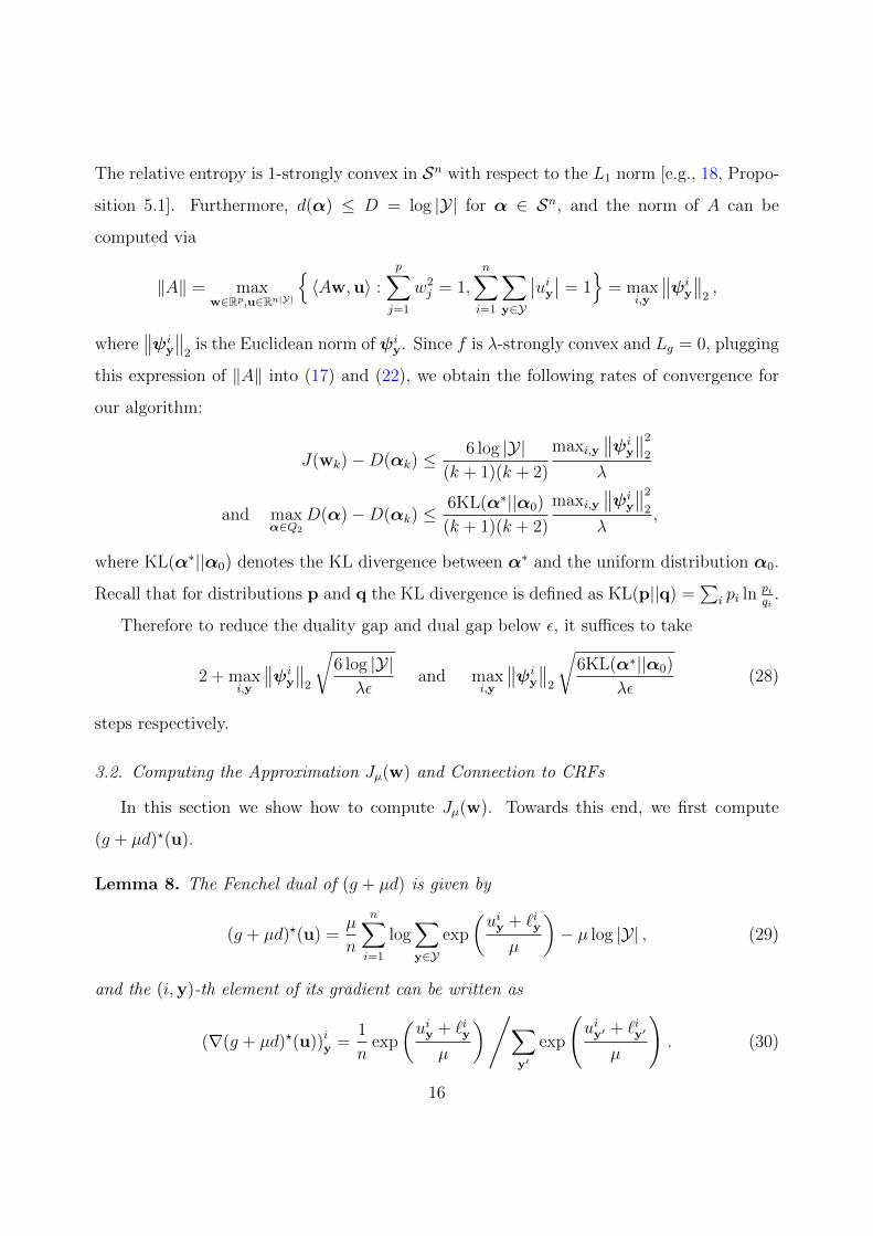
The relative entropy is 1-strongly convex in Sn with respect to the L1 norm [e.g., 18, Propo-

sition 5.1]. Furthermore, d(α) ≤ D = log |Y| for α ∈ Sn, and the norm of A can be

computed via

‖A‖ = maxw∈Rp,u∈Rn|Y|

〈Aw,u〉 :

p∑j=1

w2j = 1,

n∑i=1

∑y∈Y

∣∣uiy∣∣ = 1

= maxi,y

∥∥ψiy

∥∥2,

where∥∥ψi

y

∥∥2

is the Euclidean norm of ψiy. Since f is λ-strongly convex and Lg = 0, plugging

this expression of ‖A‖ into (17) and (22), we obtain the following rates of convergence for

our algorithm:

J(wk)−D(αk) ≤6 log |Y|

(k + 1)(k + 2)

maxi,y∥∥ψi

y

∥∥2

2

λ

and maxα∈Q2

D(α)−D(αk) ≤6KL(α∗||α0)

(k + 1)(k + 2)

maxi,y∥∥ψi

y

∥∥2

2

λ,

where KL(α∗||α0) denotes the KL divergence between α∗ and the uniform distribution α0.

Recall that for distributions p and q the KL divergence is defined as KL(p||q) =∑

i pi lnpiqi

.

Therefore to reduce the duality gap and dual gap below ε, it suffices to take

2 + maxi,y

∥∥ψiy

∥∥2

√6 log |Y|λε

and maxi,y

∥∥ψiy

∥∥2

√6KL(α∗||α0)

λε(28)

steps respectively.

3.2. Computing the Approximation Jµ(w) and Connection to CRFs

In this section we show how to compute Jµ(w). Towards this end, we first compute

(g + µd)?(u).

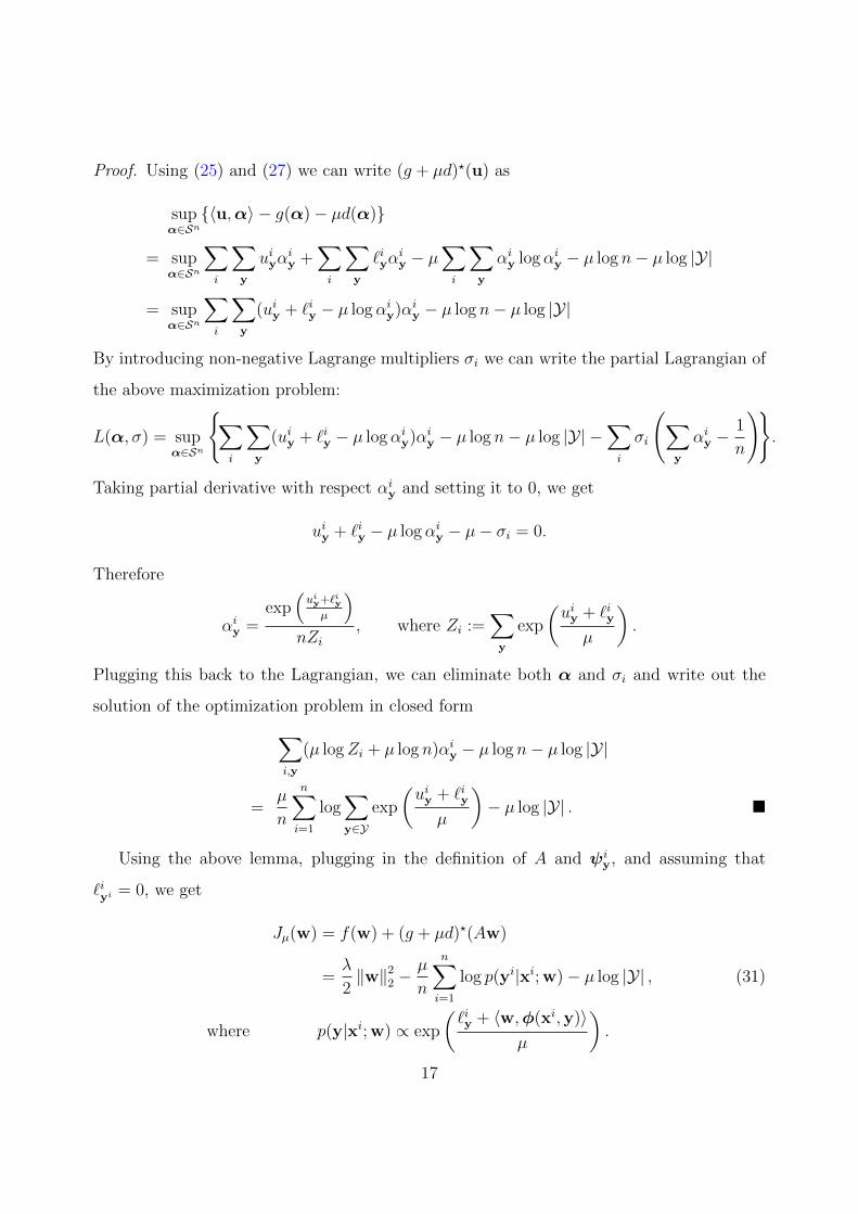
Lemma 8. The Fenchel dual of (g + µd) is given by

(g + µd)?(u) =µ

n

n∑i=1

log∑y∈Y

exp

(uiy + `iy

µ

)− µ log |Y| , (29)

and the (i,y)-th element of its gradient can be written as

(∇(g + µd)?(u))iy =1

nexp

(uiy + `iy

µ

)/∑y′

exp

(uiy′ + `iy′

µ

). (30)

16

Proof. Using (25) and (27) we can write (g + µd)?(u) as

supα∈Sn〈u,α〉 − g(α)− µd(α)

= supα∈Sn

∑i

∑y

uiyαiy +

∑i

∑y

`iyαiy − µ

∑i

∑y

αiy logαiy − µ log n− µ log |Y|

= supα∈Sn

∑i

∑y

(uiy + `iy − µ logαiy)αiy − µ log n− µ log |Y|

By introducing non-negative Lagrange multipliers σi we can write the partial Lagrangian of

the above maximization problem:

L(α, σ) = supα∈Sn

∑i

∑y

(uiy + `iy − µ logαiy)αiy − µ log n− µ log |Y| −∑i

σi

(∑y

αiy −1

n

).

Taking partial derivative with respect αiy and setting it to 0, we get

uiy + `iy − µ logαiy − µ− σi = 0.

Therefore

αiy =exp

(uiy+`iyµ

)nZi

, where Zi :=∑y

exp

(uiy + `iy

µ

).

Plugging this back to the Lagrangian, we can eliminate both α and σi and write out the

solution of the optimization problem in closed form∑i,y

(µ logZi + µ log n)αiy − µ log n− µ log |Y|

=µ

n

n∑i=1

log∑y∈Y

exp

(uiy + `iy

µ

)− µ log |Y| .

Using the above lemma, plugging in the definition of A and ψiy, and assuming that

`iyi = 0, we get

Jµ(w) = f(w) + (g + µd)?(Aw)

=λ

2‖w‖2

2 −µ

n

n∑i=1

log p(yi|xi; w)− µ log |Y| , (31)

where p(y|xi; w) ∝ exp

(`iy + 〈w,φ(xi,y)〉

µ

).

17

This interpretation clearly shows that the approximation Jµ(w) essentially converts the

maximum margin estimation problem (2) into a CRF estimation problem (1). Here µ

determines the quality of the approximation; when µ → 0, p(y|xi; w) tends to the delta

distribution with the probability mass concentrated on argmaxy `iy + 〈w,φ(xi,y)〉. Besides,

the loss `iy rescales the distribution.

Given the above interpretation, it is tempting to argue that every non-smooth problem

can be solved by computing a smooth approximation Jµ(w), and applying a standard smooth

convex optimizer to minimize Jµ(w). Unfortunately, this approach is fraught with problems.

In order to get a close enough approximation of J(w) the µ needs to be set to a very small

number which makes Jµ(w) ill-conditioned and leads to numerical issues in the optimizer.

The excessive gap technique adaptively changes the µ in each iteration in order to avoid

these problems.

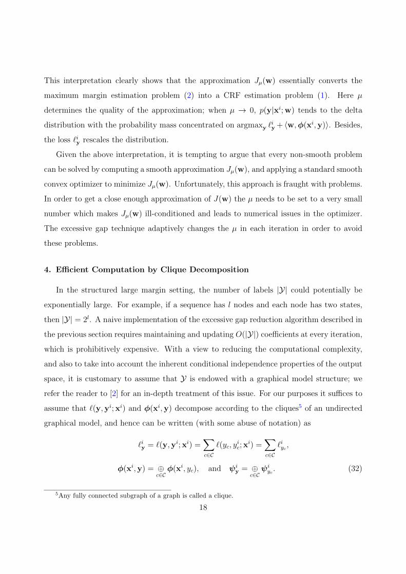
4. Efficient Computation by Clique Decomposition

In the structured large margin setting, the number of labels |Y| could potentially be

exponentially large. For example, if a sequence has l nodes and each node has two states,

then |Y| = 2l. A naive implementation of the excessive gap reduction algorithm described in

the previous section requires maintaining and updating O(|Y|) coefficients at every iteration,

which is prohibitively expensive. With a view to reducing the computational complexity,

and also to take into account the inherent conditional independence properties of the output

space, it is customary to assume that Y is endowed with a graphical model structure; we

refer the reader to [2] for an in-depth treatment of this issue. For our purposes it suffices to

assume that `(y,yi; xi) and φ(xi,y) decompose according to the cliques5 of an undirected

graphical model, and hence can be written (with some abuse of notation) as

`iy = `(y,yi; xi) =∑c∈C

`(yc, yic; x

i) =∑c∈C

`iyc ,

φ(xi,y) = ⊕c∈Cφ(xi, yc), and ψi

y = ⊕c∈Cψiyc . (32)

5Any fully connected subgraph of a graph is called a clique.

18

Figure 3: Graphical model of a linear chain. Circles indicate cliques.

Here C denotes the set of all cliques of the graphical model and ⊕ denotes vector concate-

nation. More explicitly, ψiy is the vector on the graphical model obtained by accumulating

the vector ψiyc on all the cliques c of the graph.

Let hc(yc) be an arbitrary real valued function on the value of y restricted to clique c.

Graphical models define a distribution p(y) on y ∈ Y whose density takes the following

factorized form:

p(y) ∝ q(y) =∏c∈C

exp (hc(yc)) . (33)

The key advantage of a graphical model is that the marginals on the cliques can be efficiently

computed:

myc :=∑

z:z|c=yc

q(z) =∑

z:z|c=yc

∏c′∈C

exp (hc′(zc′)) .

where the summation is over all the configurations z in Y whose restriction on the clique c

equals yc. Although Y can be exponentially large, efficient dynamic programming algorithms

exist that exploit the factorized form (33), e.g. belief propagation [19]. The computational

cost is O(sωN) where s is the number of states of each node, ω is the maximum size of the

cliques, and N is the number of cliques. For example, a linear chain as shown in Figure

3 has ω = 2 and the cliques are just edges between consecutive nodes. When ω is large,

approximate algorithms also exist [20, 21, 22]. In the sequel we will assume that our graphical

models are tractable, i.e., ω is low. The key technique that keeps our algorithm tractable

is to reformulate all updates in terms of the marginal distribution on the cliques, which is

similar in vein to the exponentiated gradient algorithm [8].

19

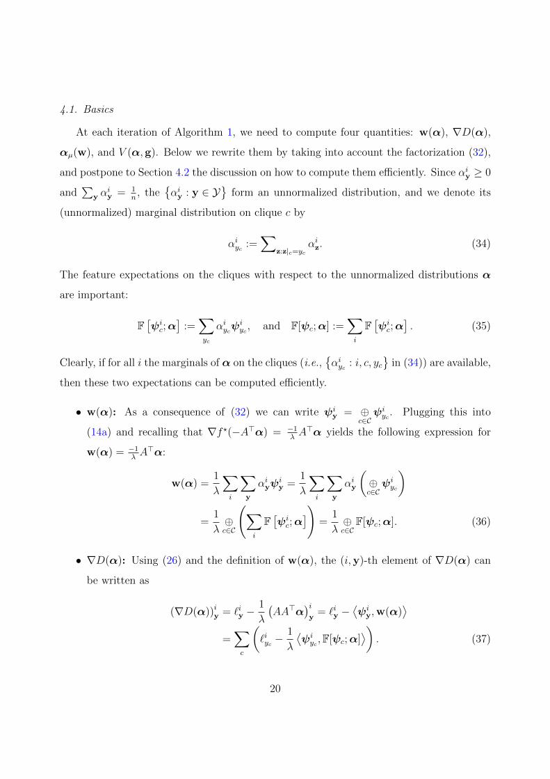
4.1. Basics

At each iteration of Algorithm 1, we need to compute four quantities: w(α), ∇D(α),

αµ(w), and V (α,g). Below we rewrite them by taking into account the factorization (32),

and postpone to Section 4.2 the discussion on how to compute them efficiently. Since αiy ≥ 0

and∑

y αiy = 1

n, the

αiy : y ∈ Y

form an unnormalized distribution, and we denote its

(unnormalized) marginal distribution on clique c by

αiyc :=∑

z:z|c=ycαiz. (34)

The feature expectations on the cliques with respect to the unnormalized distributions α

are important:

F[ψic;α]

:=∑yc

αiycψiyc , and F[ψc;α] :=

∑i

F[ψic;α]. (35)

Clearly, if for all i the marginals of α on the cliques (i.e.,αiyc : i, c, yc

in (34)) are available,

then these two expectations can be computed efficiently.

• w(α): As a consequence of (32) we can write ψiy = ⊕

c∈Cψiyc . Plugging this into

(14a) and recalling that ∇f ?(−A>α) = −1λA>α yields the following expression for

w(α) = −1λA>α:

w(α) =1

λ

∑i

∑y

αiyψiy =

1

λ

∑i

∑y

αiy

(⊕c∈Cψiyc

)

=1

λ⊕c∈C

(∑i

F[ψic;α])

=1

λ⊕c∈C

F[ψc;α]. (36)

• ∇D(α): Using (26) and the definition of w(α), the (i,y)-th element of ∇D(α) can

be written as

(∇D(α))iy = `iy −1

λ

(AA>α

)iy

= `iy −⟨ψi

y,w(α)⟩

=∑c

(`iyc −

1

λ

⟨ψiyc ,F[ψc;α]

⟩). (37)

20

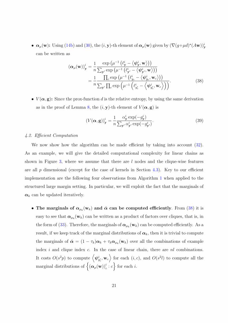
• αµ(w): Using (14b) and (30), the (i,y)-th element ofαµ(w) given by (∇(g+µd)?(Aw))iy

can be written as

(αµ(w))iy =1

n

exp(µ−1

(`iy −

⟨ψi

y,w⟩))∑

y′ exp(µ−1

(`iy′ −

⟨ψi

y′ ,w⟩))

=1

n

∏c exp

(µ−1

(`iyc −

⟨ψiyc ,wc

⟩))∑

y′∏

c exp(µ−1

(`iy′c −

⟨ψiy′c,wc

⟩)) . (38)

• V (α,g): Since the prox-function d is the relative entropy, by using the same derivation

as in the proof of Lemma 8, the (i,y)-th element of V (α,g) is

(V (α,g))iy =1

n

αiy exp(−giy)∑y′ αiy′ exp(−giy′)

. (39)

4.2. Efficient Computation

We now show how the algorithm can be made efficient by taking into account (32).

As an example, we will give the detailed computational complexity for linear chains as

shown in Figure 3, where we assume that there are l nodes and the clique-wise features

are all p dimensional (except for the case of kernels in Section 4.3). Key to our efficient

implementation are the following four observations from Algorithm 1 when applied to the

structured large margin setting. In particular, we will exploit the fact that the marginals of

αk can be updated iteratively.

• The marginals of αµk(wk) and α can be computed efficiently. From (38) it is

easy to see that αµk(wk) can be written as a product of factors over cliques, that is, in

the form of (33). Therefore, the marginals ofαµk(wk) can be computed efficiently. As a

result, if we keep track of the marginal distributions of αk, then it is trivial to compute

the marginals of α = (1 − τk)αk + τkαµk(wk) over all the combinations of example

index i and clique index c. In the case of linear chain, there are nl combinations.

It costs O(s2p) to compute⟨ψiy′c,wc

⟩for each (i, c), and O(s2l) to compute all the

marginal distributions of

(αµ(w))ic : c

for each i.

21

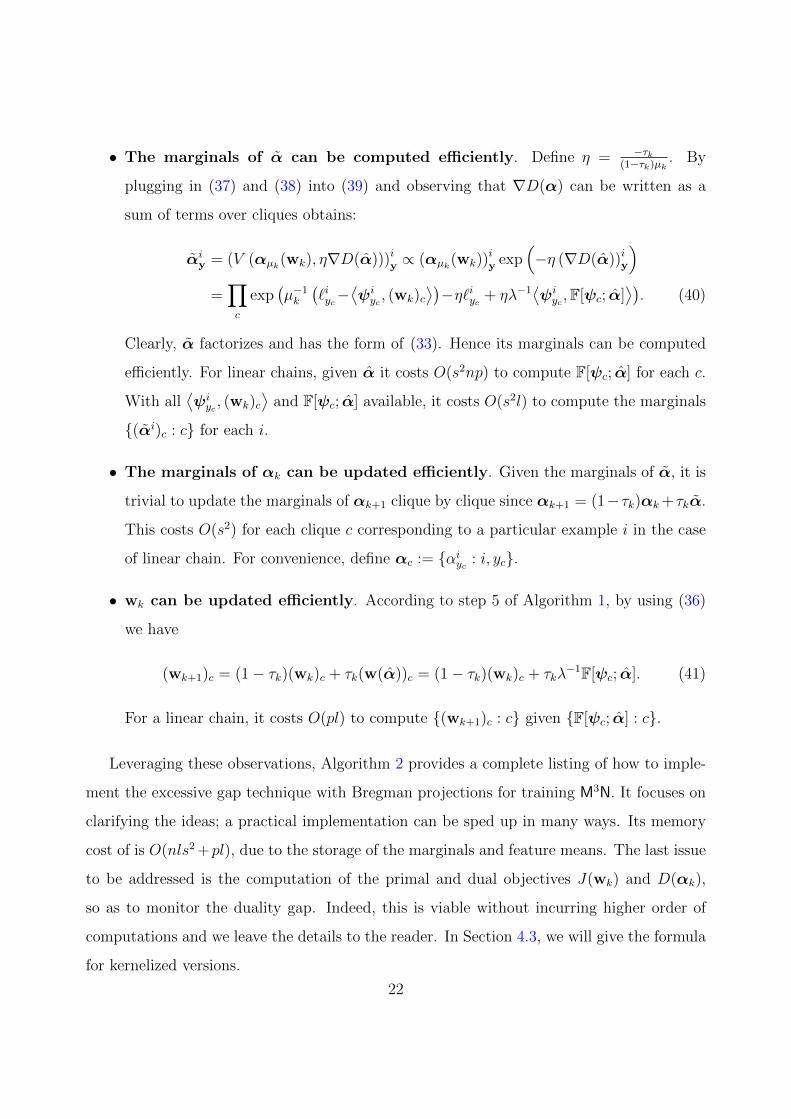
• The marginals of α can be computed efficiently. Define η = −τk(1−τk)µk

. By

plugging in (37) and (38) into (39) and observing that ∇D(α) can be written as a

sum of terms over cliques obtains:

αiy = (V (αµk(wk), η∇D(α)))iy ∝ (αµk(wk))iy exp

(−η (∇D(α))iy

)=∏c

exp(µ−1k

(`iyc−

⟨ψiyc , (wk)c

⟩)−η`iyc + ηλ−1

⟨ψiyc ,F[ψc; α]

⟩). (40)

Clearly, α factorizes and has the form of (33). Hence its marginals can be computed

efficiently. For linear chains, given α it costs O(s2np) to compute F[ψc; α] for each c.

With all⟨ψiyc , (wk)c

⟩and F[ψc; α] available, it costs O(s2l) to compute the marginals

(αi)c : c for each i.

• The marginals of αk can be updated efficiently. Given the marginals of α, it is

trivial to update the marginals of αk+1 clique by clique since αk+1 = (1−τk)αk +τkα.

This costs O(s2) for each clique c corresponding to a particular example i in the case

of linear chain. For convenience, define αc := αiyc : i, yc.

• wk can be updated efficiently. According to step 5 of Algorithm 1, by using (36)

we have

(wk+1)c = (1− τk)(wk)c + τk(w(α))c = (1− τk)(wk)c + τkλ−1F[ψc; α]. (41)

For a linear chain, it costs O(pl) to compute (wk+1)c : c given F[ψc; α] : c.

Leveraging these observations, Algorithm 2 provides a complete listing of how to imple-

ment the excessive gap technique with Bregman projections for training M3N. It focuses on

clarifying the ideas; a practical implementation can be sped up in many ways. Its memory

cost of is O(nls2 +pl), due to the storage of the marginals and feature means. The last issue

to be addressed is the computation of the primal and dual objectives J(wk) and D(αk),

so as to monitor the duality gap. Indeed, this is viable without incurring higher order of

computations and we leave the details to the reader. In Section 4.3, we will give the formula

for kernelized versions.

22

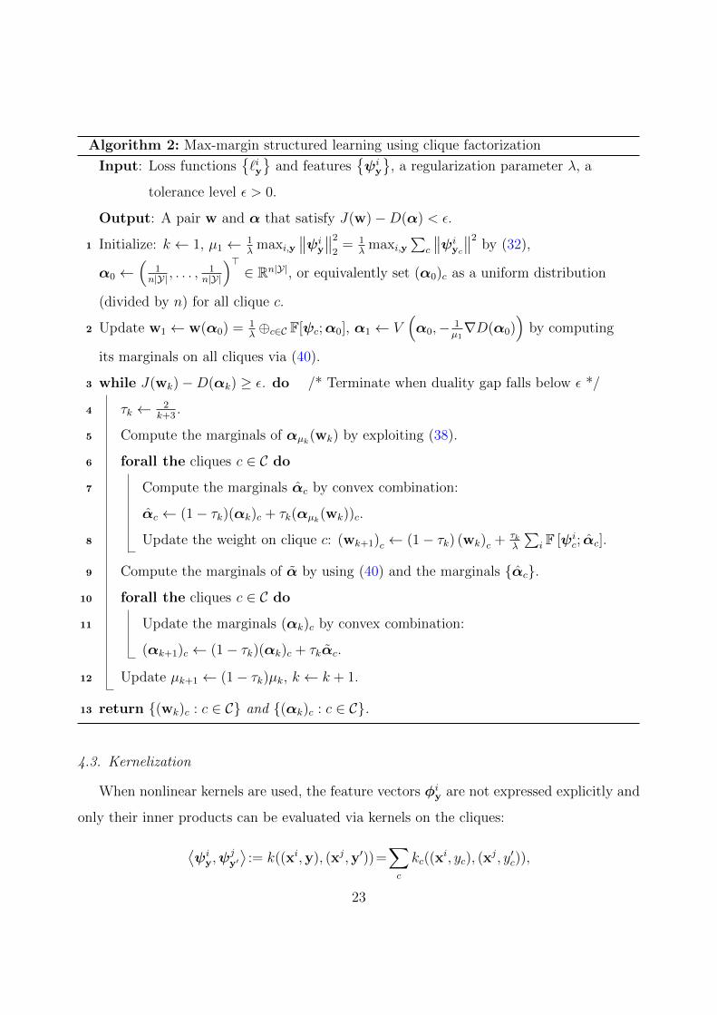
Algorithm 2: Max-margin structured learning using clique factorization

Input: Loss functions`iy

and featuresψi

y

, a regularization parameter λ, a

tolerance level ε > 0.

Output: A pair w and α that satisfy J(w)−D(α) < ε.

1 Initialize: k ← 1, µ1 ← 1λ

maxi,y∥∥ψi

y

∥∥2

2= 1

λmaxi,y

∑c

∥∥ψiyc

∥∥2by (32),

α0 ←(

1n|Y| , . . . ,

1n|Y|

)>∈ Rn|Y|, or equivalently set (α0)c as a uniform distribution

(divided by n) for all clique c.

2 Update w1 ← w(α0) = 1λ⊕c∈C F[ψc;α0], α1 ← V

(α0,− 1

µ1∇D(α0)

)by computing

its marginals on all cliques via (40).

3 while J(wk)−D(αk) ≥ ε. do /* Terminate when duality gap falls below ε */

4 τk ← 2k+3

.

5 Compute the marginals of αµk(wk) by exploiting (38).

6 forall the cliques c ∈ C do

7 Compute the marginals αc by convex combination:

αc ← (1− τk)(αk)c + τk(αµk(wk))c.

8 Update the weight on clique c: (wk+1)c ← (1− τk) (wk)c + τkλ

∑i F [ψi

c; αc].

9 Compute the marginals of α by using (40) and the marginals αc.

10 forall the cliques c ∈ C do

11 Update the marginals (αk)c by convex combination:

(αk+1)c ← (1− τk)(αk)c + τkαc.

12 Update µk+1 ← (1− τk)µk, k ← k + 1.

13 return (wk)c : c ∈ C and (αk)c : c ∈ C.

4.3. Kernelization

When nonlinear kernels are used, the feature vectors φiy are not expressed explicitly and

only their inner products can be evaluated via kernels on the cliques:

⟨ψi

y,ψjy′

⟩:= k((xi,y), (xj,y′))=

∑c

kc((xi, yc), (x

j, y′c)),

23

where kc((xi, yc), (x

j, y′c)) :=⟨ψiyc ,ψ

jy′c

⟩. Algorithm 2 is no longer applicable because no

explicit expression of w is available. However, by rewriting wk as the feature expectations

with respect to some distribution βk ∈ Sn, then we only need to update wk implicitly via βk,

and the inner product between wk and any feature vector can also be efficiently calculated.

We formalize and prove this claim by induction.

Theorem 9. For all k ≥ 0, there exists βk ∈ Sn, such that (wk)c = 1λF[ψc;βk], and βk can

be updated by βk+1 = (1− τk)βk + τkαk.

Proof. First, w1 = w(α0) = 1λ⊕c∈C F[ψc;α0], so β1 = α0. Suppose the claim holds for all

1, . . . , k, then

(wk+1)c = (1−τk)(wk)c +τkλF[ψc; (αk)c] = (1−τk)

1

λF[ψc;βk]+

τkλF[ψc; (αk)c]

=1

λF[ψc; (1− τk)(βk)c+τk(αk)c].

Therefore, we can set βk+1 = (1− τk)βk + τkαk ∈ Sn.

In general αk 6= αk, hence βk 6= αk. To compute⟨ψiyc , (wk)c

⟩required by (40), we have

⟨ψiyc , (wk)c

⟩=

⟨ψiyc ,

1

λ

∑j

∑y′c

βjy′cψjy′c

⟩=

1

λ

∑j

∑y′c

βjy′ckc((xi, yc), (x

j, y′c)).

And by using this trick, all the iterative updates in Algorithm 2 can be done efficiently. So

is the evaluation of ‖wk‖2 and the primal objective. The dual objective (26) is also easy

since∑i

∑y

`iy(αk)iy =

∑i

∑y

∑c

`iyc(αk)iy =

∑i

∑c

∑yc

`iyc

∑y:y|c=yc

(αk)iy =

∑i,c,yc

`iyc(αk)iyc ,

and the marginals of αk are available. Finally, the quadratic term in D(αk) can be computed

by ∥∥A>αk∥∥2

2=∥∥∑

i,y

ψiy(αk)

iy

∥∥2

2=∑c

∥∥∑i,yc

ψiyc(αk)

iyc

∥∥2

2

=∑c

∑i,j,yc,y′c

(αk)iyc(αk)

jy′ckc((x

i, yc), (xj, y′c)),

24

where the inner term is the same as the unnormalized expectation that can be efficiently

calculated. The last formula is only for nonlinear kernels.

Note for nonlinear kernels, the computational cost can be shown to be O(n2ls2).

5. Discussion

Structured output prediction is an important learning task in both theory and practice.

The main contribution of our paper is twofold. First, we identified an efficient algorithm

by Nesterov [1] for solving the optimization problems in structured prediction. We proved

the O(1/√ε) rate of convergence for the Bregman projection based updates in excessive gap

optimization, while Nesterov [1] showed this rate only for projected gradient style updates.

In M3N optimization, Bregman projection plays a key role in factorizing the computations,

while technically such factorizations are not applicable to projected gradient. Second, we

designed a nontrivial application of the excessive gap technique to M3N optimization, in

which the computations are kept efficient by using the graphical model decomposition. Ker-

nelized objectives can also be handled by our method, and we proved superior convergence

and computational guarantees than existing algorithms.

When M3Ns are trained in a batch fashion, we can compare the convergence rate of dual

gap between our algorithm and the exponentiated gradient method [ExpGrad, 8]. Assume

α0, the initial value of α, is the uniform distribution and α∗ is the optimal dual solution.

Then by (28), we have

Ours: maxi,y

∥∥ψiy

∥∥2

√6KL(α∗||α0)

λε, ExpGrad: max

i,y

∥∥ψiy

∥∥2

2

KL(α∗||α0)

λε.

It is clear that our iteration bound is almost the square root of ExpGrad, and has much

better dependence on ε, λ, maxi,y∥∥ψi

y

∥∥2, as well as the divergence from the initial guess to

the optimal solution KL(α∗||α0).

In addition, the cost per iteration of our algorithm is almost the same as ExpGrad, and

both are governed by the computation of the expected feature values on the cliques (which

we call exp-oracle), or equivalently the marginal distributions. For graphical models, ex-

act inference algorithms such as belief propagation can compute the marginals via dynamic

25

programming [19]. Finally, although both algorithms require marginalization, they are cal-

culated in very different ways. In ExpGrad, the dual variables α correspond to a factorized

distribution, and in each iteration its potential functions on the cliques are updated using

the exponentiated gradient rule. In contrast, our algorithm explicitly updates the marginal

distributions of αk on the cliques, and marginalization inference is needed only for α and

α. Indeed, the joint distribution α does not factorize, which can be seen from step 7

of Algorithm 1: the convex combination of two factorized distributions is not necessarily

factorized.

Marginalization is just one type of query that can be answered efficiently by graphical

models, and another important query is the max a-posteriori inference (which we call max-

oracle): given the current model w, find the argmax in (2). Max-oracle has been used by

greedy algorithms such as cutting plane (BMRM and SVM-Struct) and sequential minimal

optimization [SMO, 9, Chapter 6]. SMO picks the steepest descent coordinate in the dual and

greedily optimizes the quadratic analytically, but its convergence rate is linear in |Y| which

can be exponentially large for M3N (ref Table 1). The max-oracle again relies on graphical

models for dynamical programming [22], and many existing combinatorial optimizers can

also be used, such as in the applications of matching [23] and context free grammar parsing

[24]. Furthermore, this oracle is particularly useful for solving the slack rescaling variant of

M3N proposed by [6]:

J(w)=λ

2‖w‖2

2+1

n

n∑i=1

maxy∈Y

`(y,yi; xi)

(1−⟨w,φ(xi,yi)− φ(xi,y)

⟩). (42)

Here two factorized terms get multiplied, which causes additional complexity in finding the

maximizer. [25, Section 1.4.1] solved this problem by a modified dynamic program. Never-

theless, it is not clear how ExpGrad or our method can be used to optimize this objective.

In the quest for faster optimization algorithms for M3Ns, the following three questions

are important: how hard is it to optimize M3N intrinsically, how informative is the oracle

which is the only way for the algorithm to access the objective function, and how well does

the algorithm make use of such information. In the oracle-optimizer model proposed in [14],

a solver can access the target objective only through an oracle, e.g., the function value and

26

its derivative at a given point. Cutting plane methods [6] and bundle methods [5] use a

max-oracle, i.e. given a query point wk, the only information available to the solver about

the objective (2) is the linear piece determined by the label y that “wins” in the maxy∈Y ,

while all other linear pieces are ignored. In contrast, our algorithm essentially endows a

distribution over all labels y as in (29), and it aggregates the information of all labels y with

respect to this distribution. Hence we call it exp-oracle (‘exp’ for expectation).

The superiority of our algorithm suggests that the exp-oracle provides more information

about the function than the max-oracle does, and a deeper explanation is that the max-

oracle is local [14, Section 1.3], i.e. it depends only on the value of the function in the

neighborhood of the querying point wk. In contrast, the exp-oracle is not local and uses

the global structure of the function. Hence there is no surprise that the less informative

max-oracle is easier to compute, which makes it applicable to a wider range of problems

such as (42). Moreover, the comparison between ExpGrad and our algorithm shows that

even if the exp-oracle is used, the algorithm still needs to make good use of it in order to

converge faster.

For future research, it is interesting to study the lower bound complexity for optimizing

M3N, including the dependence on ε, n, λ, Y , and probably even on the graphical model

topology. Empirical evaluation of our algorithm is also important, especially regarding the

numerical stability of the additive update of marginal distributions αk under fixed precision.

Broader applications are possible in sequence labeling, word alignment, context free grammar

parsing, etc.

Acknowledgements. We thank the anonymous reviewers of ALT 2011 for many insightful

comments and helpful suggestions. Xinhua Zhang would like to acknowledge support from

the Alberta Innovates Centre for Machine Learning. Ankan Saha would like to acknowledge

the fellowship support of the University of Chicago. The work of S.V.N. Vishwanathan is

partially supported by a grant from Google and NSF grant IIS-1117705.

27

References

[1] Y. Nesterov, Excessive Gap Technique in Nonsmooth Convex Minimization, SIAM Journal on Opti-

mization 16 (1) (2005) 235–249.

[2] G. Bakir, T. Hofmann, B. Scholkopf, A. Smola, B. Taskar, S. V. N. Vishwanathan, Predicting Structured

Data, MIT Press, 2007.

[3] J. D. Lafferty, A. McCallum, F. Pereira, Conditional Random Fields: Probabilistic Modeling for Seg-

menting and Labeling Sequence Data, in: Proceedings of International Conference on Machine Learning,

2001.

[4] B. Taskar, C. Guestrin, D. Koller, Max-Margin Markov Networks, in: Advances in Neural Information

Processing Systems 16, 2004.

[5] C. Teo, S. Vishwanthan, A. Smola, Q. Le, Bundle Methods for Regularized Risk Minimization, Journal

of Machine Learning Research 11 (2010) 311–365.

[6] I. Tsochantaridis, T. Joachims, T. Hofmann, Y. Altun, Large Margin Methods for Structured and

Interdependent Output Variables, Journal of Machine Learning Research 6 (2005) 1453–1484.

[7] B. Taskar, S. Lacoste-Julien, M. Jordan, Structured Prediction, Dual Extragradient and Bregman

Projections, Journal of Machine Learning Research 7 (2006) 1627–1653.

[8] M. Collins, A. Globerson, T. Koo, X. Carreras, P. Bartlett, Exponentiated Gradient Algorithms for

Conditional Random Fields and Max-Margin Markov Networks, Journal of Machine Learning Research

9 (2008) 1775–1822.

[9] B. Taskar, Learning Structured Prediction Models: A Large Margin Approach, Ph.D. thesis, Stanford

University, 2004.

[10] N. List, H. U. Simon, SVM-Optimization and Steepest-Descent Line Search, in: Proceedings of the

Annual Conference on Computational Learning Theory, 2009.

[11] F. Sha, F. Pereira, Shallow Parsing with Conditional Random Fields, in: Proceedings of HLT-NAACL,

2003.

[12] S. Boyd, L. Vandenberghe, Convex Optimization, Cambridge University Press, Cambridge, England,

2004.

[13] T. Joachims, T. Finley, C.-N. J. Yu, Cutting-Plane Training of Structural SVMs, Machine Learning

77 (1) (2009) 27–59.

[14] A. Nemirovski, D. Yudin, Problem Complexity and Method Efficiency in Optimization, John Wiley

and Sons, 1983.

[15] Y. Nesterov, Smooth minimization of non-smooth functions, Mathematical Programming 103 (1) (2005)

127–152.

[16] J. Hiriart-Urruty, C. Lemarechal, Convex Analysis and Minimization Algorithms, I and II, vol. 305 and

28

306, Springer-Verlag, 1993.

[17] J. M. Borwein, A. S. Lewis, Convex Analysis and Nonlinear Optimization: Theory and Examples,

Canadian Mathematical Society, 2000.

[18] A. Beck, B. Teboulle, Mirror Descent and Nonlinear Projected Subgradient Methods for Convex Opti-

mization, Operations Research Letters 31 (3) (2003) 167–175.

[19] S. L. Lauritzen, Graphical Models, Oxford University Press, Oxford, UK, 1996.

[20] M. Wainwright, M. Jordan, Graphical Models, Exponential Families, and Variational Inference, Foun-

dations and Trends in Machine Learning 1 (1–2) (2008) 1–305.

[21] C. Andrieu, N. de Freitas, A. Doucet, M. I. Jordan, An Introduction to MCMC for Machine Learning,

Machine Learning 50 (2003) 5–43.

[22] F. Kschischang, B. J. Frey, H. Loeliger, Factor Graphs and the Sum-Product Algorithm, IEEE Trans.

on Information Theory 47 (2) (2001) 498–519.

[23] B. Taskar, S. Lacoste-Julien, D. Klein, A Discriminative Matching Approach to Word Alignment, in:

Empirical Methods in Natural Language Processing, 2005.

[24] B. Taskar, D. Klein, M. Collins, D. Koller, C. Manning, Max-Margin Parsing, in: Empirical Methods

in Natural Language Processing, 2004.

[25] Y. Altun, T. Hofmann, I. Tsochandiridis, Support Vector Machine Learning for Interdependent and

Structured Output Spaces, in: G. Bakir, T. Hofmann, B. Scholkopf, A. Smola, B. Taskar, S. V. N.

Vishwanathan (Eds.), Predicting Structured Data, chap. 5, MIT Press, 85–103, 2007.

29