Inertial Navigation

Academic Year 2008/09

Master of Science in Computer Engineering,Environmental and Land Planning Engineering

Inertial navigation

• Reference systems

• Inertial sensors

• Navigation equations

• Error budget

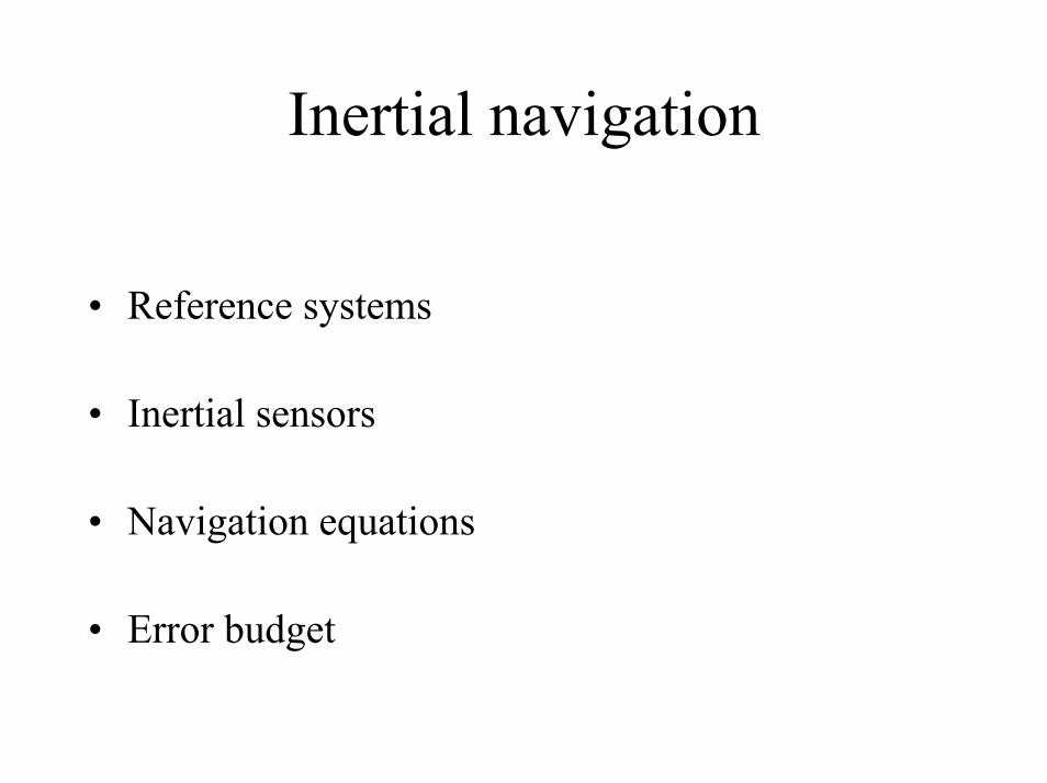
Pseudo inertial system- origin in the Earth barycentre;- x3 axis: oriented towards a celestial North Pole;- x1 axis: intersection between ecliptic and celestial equatorial plane;- x2 axis: to complete the right-handed triad.

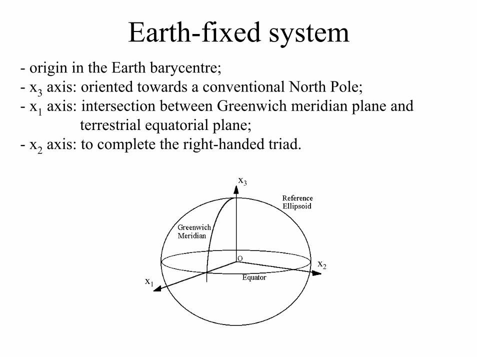
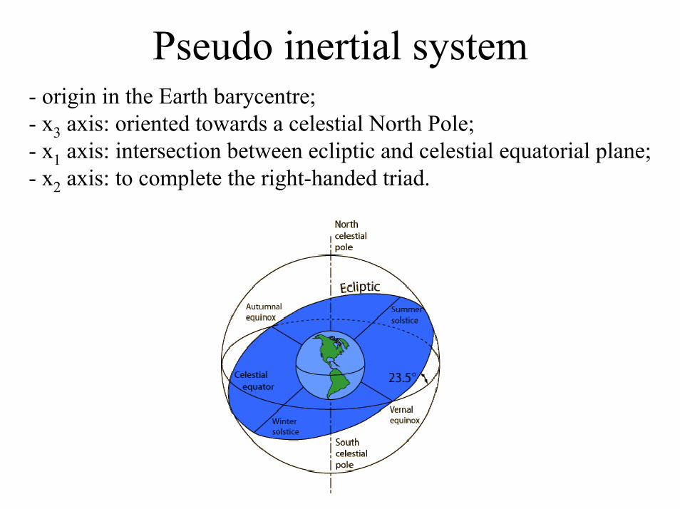
Earth-fixed system- origin in the Earth barycentre;- x3 axis: oriented towards a conventional North Pole;- x1 axis: intersection between Greenwich meridian plane and

terrestrial equatorial plane;- x2 axis: to complete the right-handed triad.

x1

x2

x3

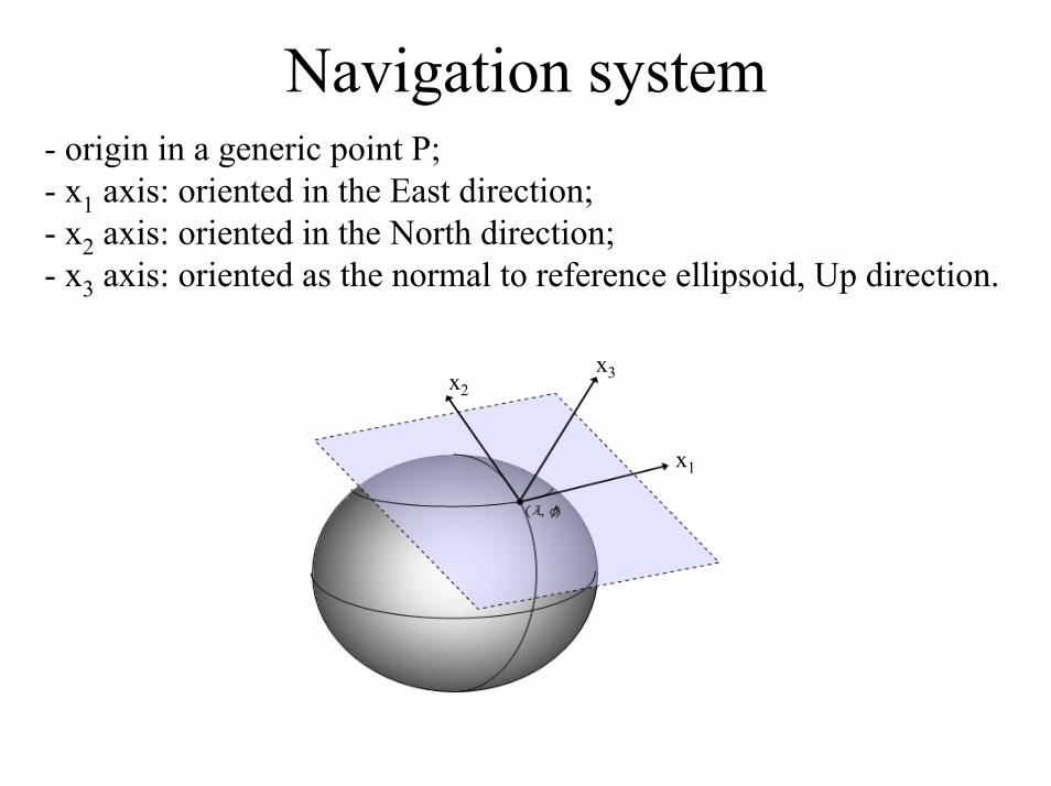
Navigation system- origin in a generic point P;- x1 axis: oriented in the East direction;- x2 axis: oriented in the North direction;- x3 axis: oriented as the normal to reference ellipsoid, Up direction.

x1

x2x3

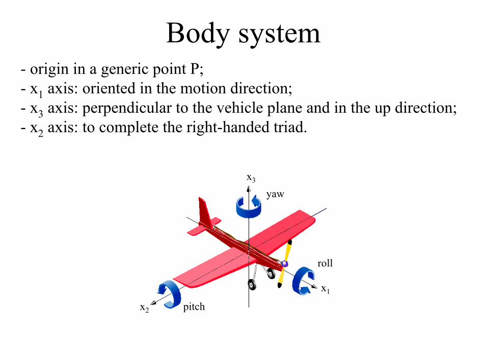
Body system- origin in a generic point P;- x1 axis: oriented in the motion direction;- x3 axis: perpendicular to the vehicle plane and in the up direction;- x2 axis: to complete the right-handed triad.

x2

x1

x3

yaw

roll

pitch

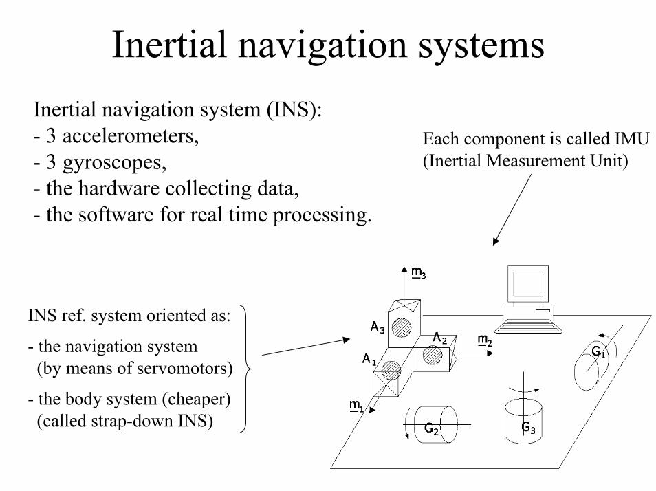
Inertial navigation systemsInertial navigation system (INS):- 3 accelerometers,- 3 gyroscopes,- the hardware collecting data,- the software for real time processing.

Each component is called IMU (Inertial Measurement Unit)

INS ref. system oriented as:

- the navigation system(by means of servomotors)

- the body system (cheaper)(called strap-down INS)

AccelerometersThe basic principle of accelerometers is to measure the forces acting on a proof mass.

Two types of accelerometers:

- open loop (e.g. spring based accelerometers)measure the displacement of the proof mass resulting from external forces acting on the sensor.

- closed loop (e.g. pendulous or electrostatic accelerometers)keep the proof mass in a state of equilibrium by generating a force that is opposite to the applied force.

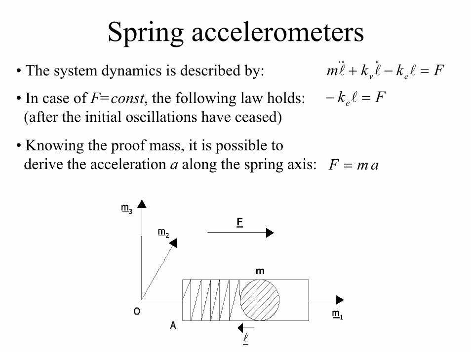
Spring accelerometers• The system dynamics is described by: Fkkm ev =−+ ll&l&&

• In case of F=const, the following law holds:(after the initial oscillations have ceased)

Fke =− l

• Knowing the proof mass, it is possible to derive the acceleration a along the spring axis: amF =

F

l

m

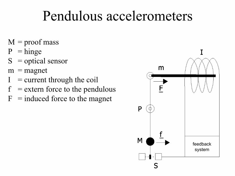
Pendulous accelerometers

M = proof massP = hingeS = optical sensorm = magnetI = current through the coilf = extern force to the pendulousF = induced force to the magnet

feedback system

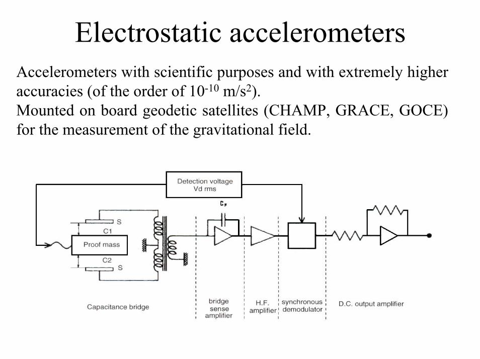
Electrostatic accelerometersAccelerometers with scientific purposes and with extremely higher accuracies (of the order of 10-10 m/s2).Mounted on board geodetic satellites (CHAMP, GRACE, GOCE) for the measurement of the gravitational field.

Accelerometer error

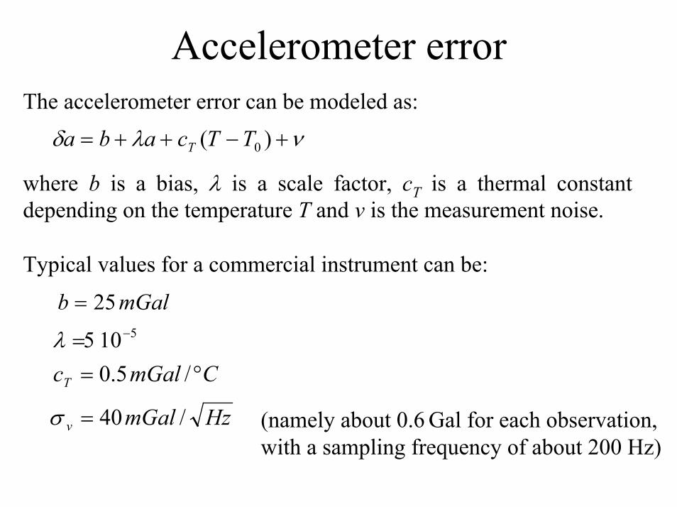
νλδ +−++= )( 0TTcaba T

The accelerometer error can be modeled as:

where b is a bias, λ is a scale factor, cT is a thermal constant depending on the temperature T and v is the measurement noise.

Typical values for a commercial instrument can be:

mGalb 25=5105 −=λ

CmGalcT °= /5.0

HzmGalv /40=σ (namely about 0.6 Gal for each observation, with a sampling frequency of about 200 Hz)

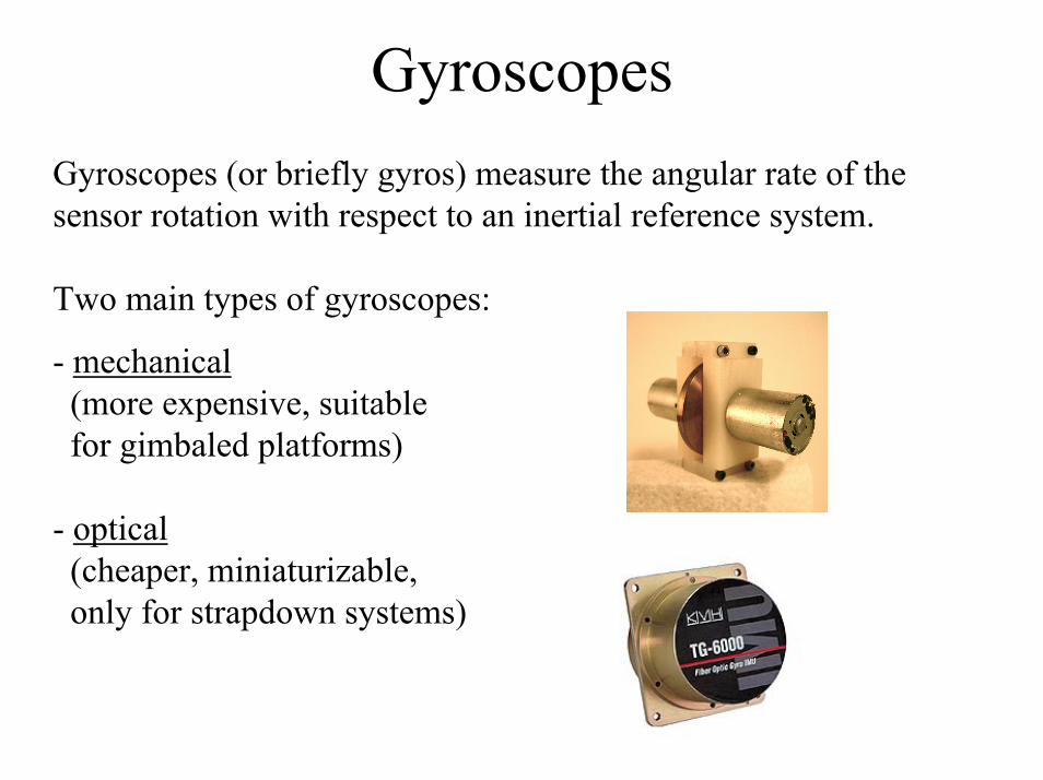
GyroscopesGyroscopes (or briefly gyros) measure the angular rate of the sensor rotation with respect to an inertial reference system.

Two main types of gyroscopes:

- mechanical(more expensive, suitable for gimbaled platforms)

- optical(cheaper, miniaturizable,only for strapdown systems)

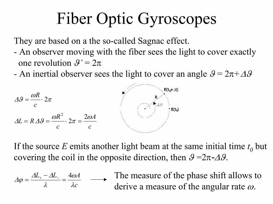
Fiber Optic GyroscopesThey are based on a the so-called Sagnac effect.- An observer moving with the fiber sees the light to cover exactly one revolution ϑ’ = 2π

- An inertial observer sees the light to cover an angle ϑ = 2π+∆ϑ

πωϑ∆ 2⋅=cR

cA

cRRL ωπωϑ∆∆ 22

2

=⋅==

If the source E emits another light beam at the same initial time t0 but covering the coil in the opposite direction, then ϑ =2π-∆ϑ.

The measure of the phase shift allows to derive a measure of the angular rate ω. c

ALLλω

λ∆∆

ϕ∆ 4=

−= −+

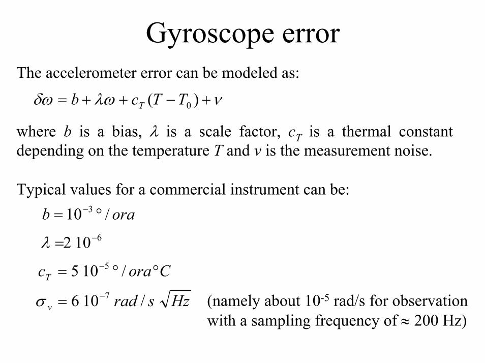
Gyroscope errorThe accelerometer error can be modeled as:

where b is a bias, λ is a scale factor, cT is a thermal constant depending on the temperature T and v is the measurement noise.

Typical values for a commercial instrument can be:

νλωδω +−++= )( 0TTcb T

orab /10 3 °= −

6102 −=λ

CoracT °°= − /105 5

(namely about 10-5 rad/s for observation with a sampling frequency of ≈ 200 Hz)

Hzsradv /106 7−=σ

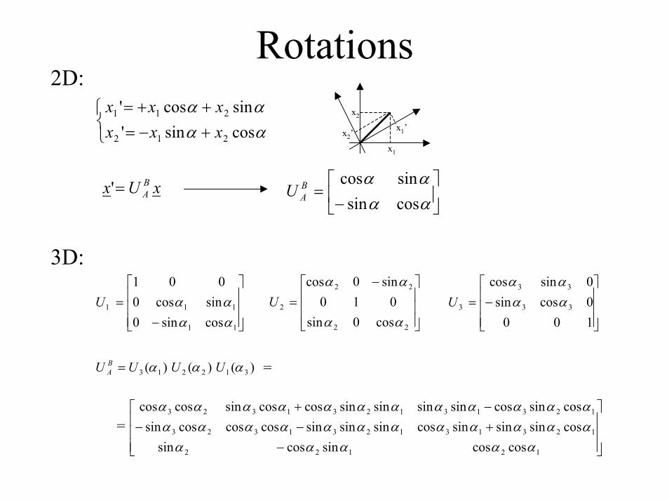
Rotations2D:

x1

x2

x1’x2’

+−=++=

αααα

cossin'sincos'

212

211

xxxxxx

−

=αααα

cossinsincosB

AUxUx BA='

3D:

−=

22

22

2

cos0sin010

sin0cos

αα

ααU

−=

11

111

cossin0sincos0

001

ααααU

−=

1000cossin0sincos

33

33

3 αααα

U

=)()()( 312213 ααα UUUU BA =

−+−−−+

12122

123131231323

123131231323

coscossincossincossinsinsincossinsinsincoscoscossincossincossinsinsinsincoscossincoscos

ααααααααααααααααααααααααααααα

=

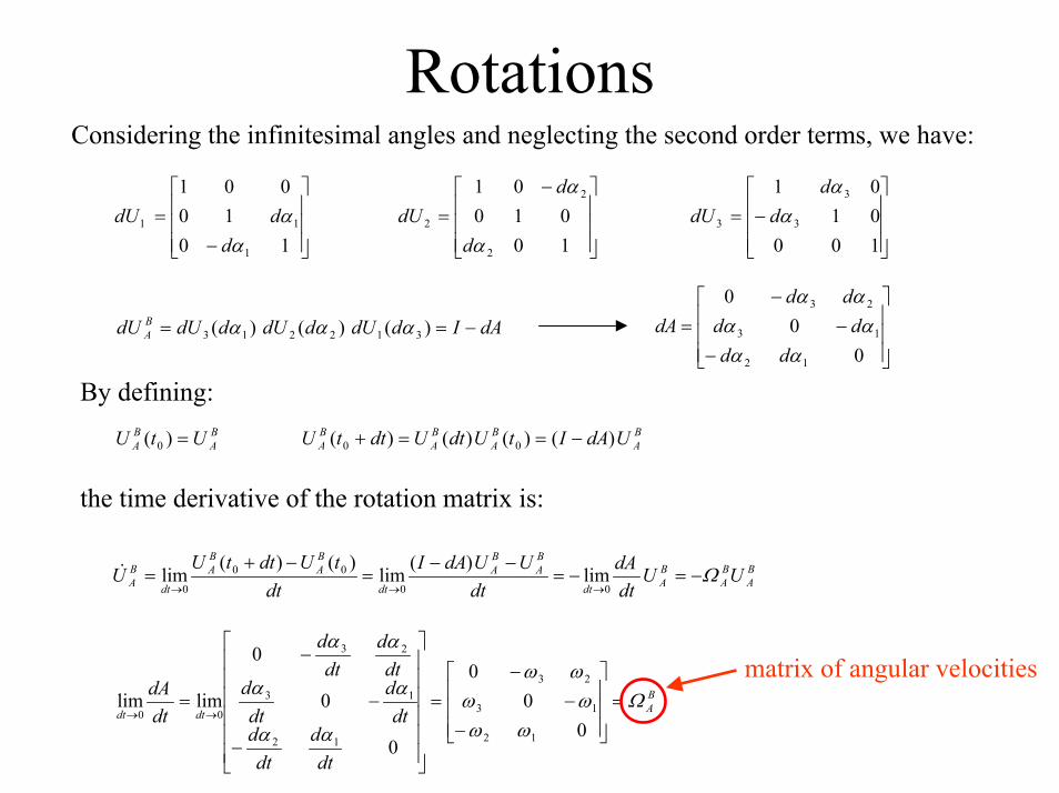
RotationsConsidering the infinitesimal angles and neglecting the second order terms, we have:

−=

1000101

3

3

3 αα

dd

dU

−=

10010

01

2

2

2

α

α

d

ddU

−=

1010

001

1

11

αα

dddU

−−

−=

00

0

12

13

23

αααααα

dddd

dddAdAIddUddUddUdU B

A −== )()()( 312213 ααα

By defining:BA

BA

BA

BA UdAItUdtUdttU )()()()( 00 −==+B

ABA UtU =)( 0

the time derivative of the rotation matrix is:

BA

BA

BAdt

BA

BA

dt

BA

BA

dt

BA UU

dtdA

dtUUdAI

dttUdttU

U Ω−=−=−−

=−+

=→→→ 00

00

0lim

)(lim

)()(lim&

BAdtdt

dtd

dtd

dtd

dtd

dtd

dtd

dtdA Ω

ωωωωωω

αα

αα

αα

=

−−

−=

−

−

−

=→→

00

0

0

0

0

limlim

12

13

23

12

13

23

00

matrix of angular velocities

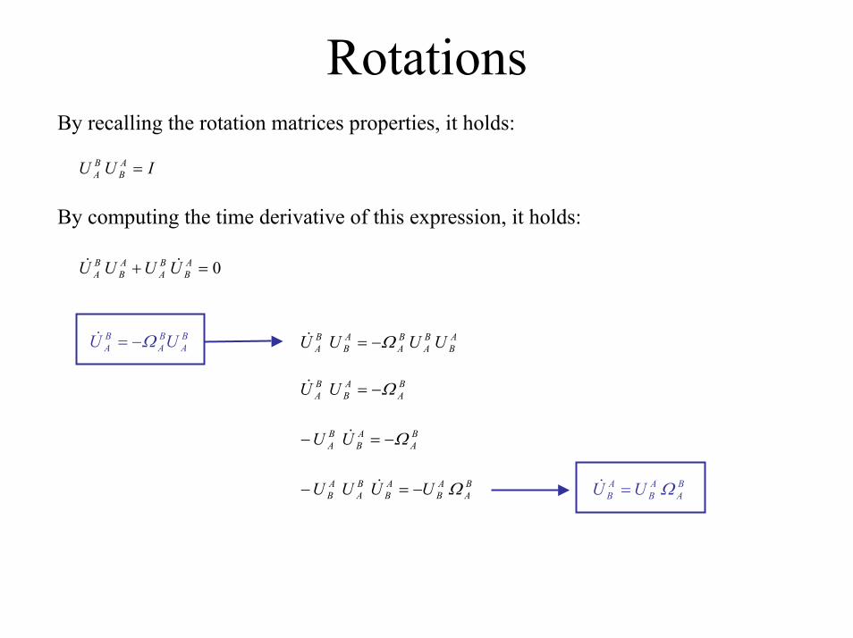
RotationsBy recalling the rotation matrices properties, it holds:

IUU AB

BA =

By computing the time derivative of this expression, it holds:

0=+ AB

BA

AB

BA UUUU &&

BA

BA

BA UU Ω−=& A

BBA

BA

AB

BA UUUU Ω−=&

BA

AB

BA UU Ω−=&

BA

AB

BA UU Ω−=− &

BA

AB

AB UU Ω=&B

AAB

AB

BA

AB UUUU Ω−=− &

Navigation equationsNavigation equations establish a link between the unknowns (namely position, velocity and attitude of the vehicle) and the observations of the accelerometers and of the gyroscopes (and in case of the GPS receivers).

Two cases:- Navigation equations in an inertial reference system

(suitable to describe space navigation, for example the orbitsof an artificial satellite)

- Navigation equations in an Earth-fixed reference system(more suitable to describe terrestrial navigation, sometimes requiring a further step towards the local-level system).

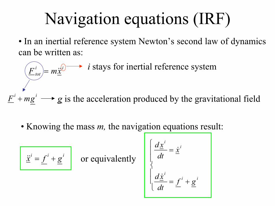
Navigation equations (IRF)• In an inertial reference system Newton’s second law of dynamics can be written as:

i stays for inertial reference systemiitot xmF &&=

ii gmF + g is the acceleration produced by the gravitational field

+=

=

iii

ii

gfdtxd

xdtxd

&

&

• Knowing the mass m, the navigation equations result:

iii gfx +=&& or equivalently

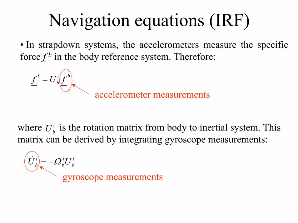
Navigation equations (IRF)• In strapdown systems, the accelerometers measure the specific force f b in the body reference system. Therefore:

bib

i fUf =

accelerometer measurements

where is the rotation matrix from body to inertial system. This matrix can be derived by integrating gyroscope measurements:

ibU

ib

ib

ib UU Ω−=&

gyroscope measurements

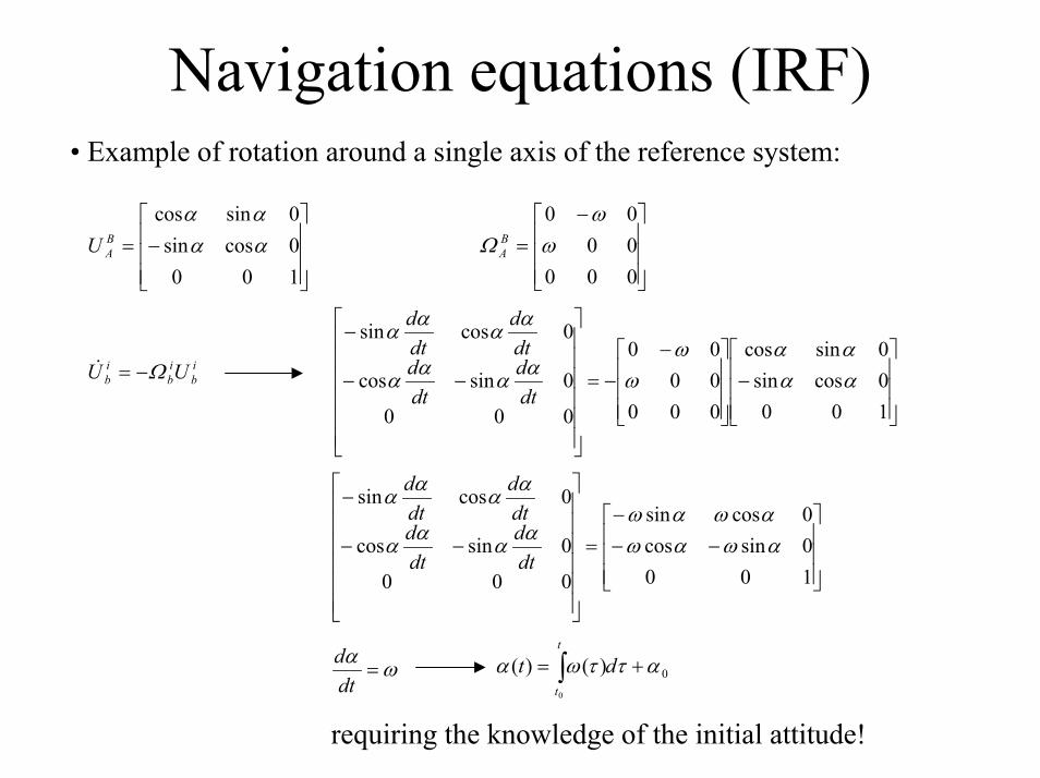
Navigation equations (IRF)• Example of rotation around a single axis of the reference system:

−=

0000000

ωω

Ω BA

−=

1000cossin0sincos

αααα

BAU

−

−−=

−−

−

1000cossin0sincos

0000000

000

0sincos

0cossin

αααα

ωω

αααα

αααα

dtd

dtd

dtd

dtd

ib

ib

ib UU Ω−=&

−−

−=

−−

−

1000sincos0cossin

000

0sincos

0cossin

αωαωαωαω

αααα

αααα

dtd

dtd

dtd

dtd

0

0

)()( αττωα += ∫ dtt

tωα

=dtd

requiring the knowledge of the initial attitude!

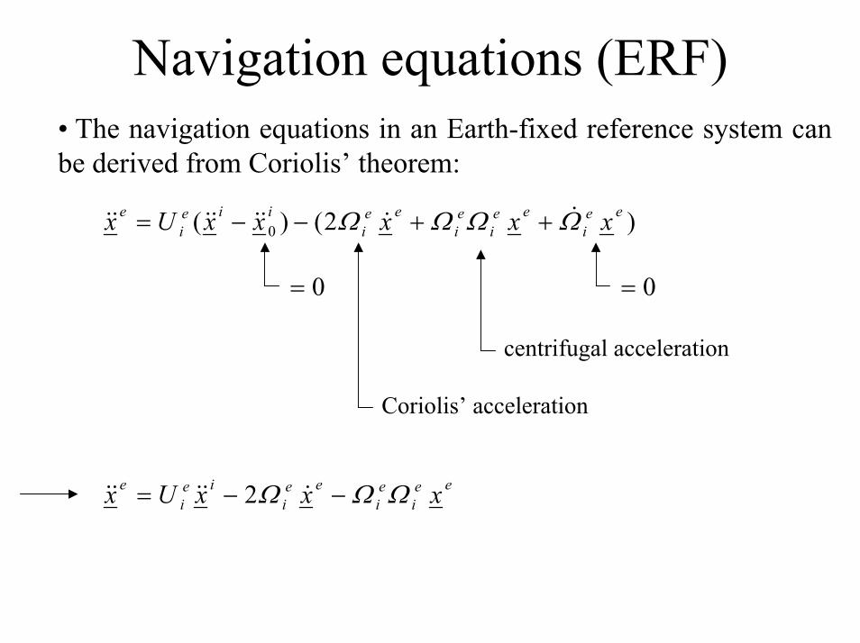
Navigation equations (ERF)• The navigation equations in an Earth-fixed reference system can be derived from Coriolis’ theorem:

)2()( 0ee

iee

iei

eei

iiei

e xxxxxUx ΩΩΩΩ &&&&&&&& ++−−=

0= 0=

centrifugal acceleration

Coriolis’ acceleration

eei

ei

eei

iei

e xxxUx ΩΩΩ −−= &&&&& 2

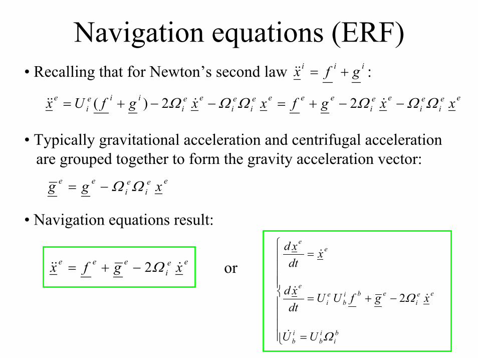
Navigation equations (ERF)• Recalling that for Newton’s second law :iii gfx +=&&

eei

ei

eei

eeeei

ei

eei

iiei

e xxgfxxgfUx ΩΩΩΩΩΩ −−+=−−+= &&&& 22)(

• Typically gravitational acceleration and centrifugal accelerationare grouped together to form the gravity acceleration vector:

eei

ei

ee xgg ΩΩ−=

eei

eee xgfx &&& Ω2−+=

=

−+=

=

bi

ib

ib

eei

ebib

ei

e

ee

UU

xgfUUdtxd

xdtxd

Ω

Ω

&

&&

&

2

• Navigation equations result:

or

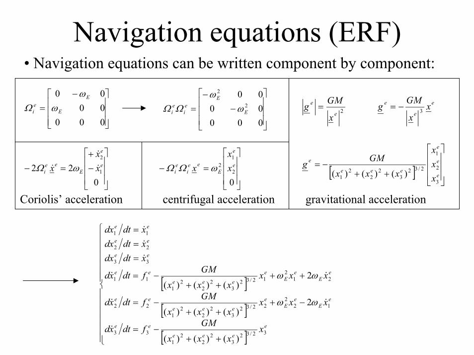
Navigation equations (ERF)• Navigation equations can be written component by component:

−=

0000000

E

Eei ω

ωΩ

−−

=0000000

2

2

E

Eei

ei ω

ωΩΩ

−+

=−0

22 1

2e

e

Eee

i xx

x &

&

& ωΩ

Coriolis’ acceleration

=−0

2

12 e

e

Eee

iei x

xx ωΩΩ

centrifugal acceleration

2e

e

x

GMg = e

e

e xx

GMg 3−=

[ ]

++−=

e

e

e

eee

e

xxx

xxxGMg

3

2

1

2/323

22

21 )()()(

gravitational acceleration

[ ]

[ ]

[ ]

++−=

−+++

−=

++++

−=

===

e

eee

ee

eE

eE

e

eee

ee

eE

eE

e

eee

ee

ee

ee

ee

xxxx

GMfdtxd

xxxxxx

GMfdtxd

xxxxxx

GMfdtxd

xdtdxxdtdxxdtdx

32/323

22

21

33

122

22/323

22

21

22

212

12/323

22

21

11

33

22

11

)()()(

2)()()(

2)()()(

&

&&

&&

&

&

&

ωω

ωω

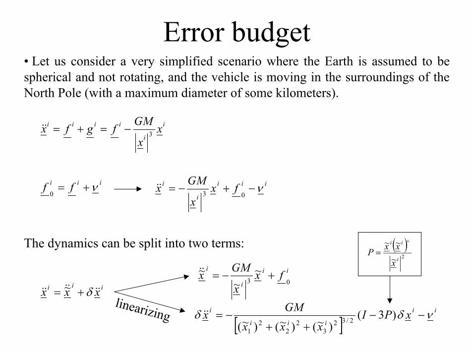
Error budget• Let us consider a very simplified scenario where the Earth is assumed to be spherical and not rotating, and the vehicle is moving in the surroundings of the North Pole (with a maximum diameter of some kilometers).

i

i

iiii xx

GMfgfx 3−=+=&&

iii

i

i fxx

GMx ν−+−=03

&&iii ff ν+=

0

ii

i

ifx

x

GMx03

~~

~ +−=&&

[ ]ii

iii

i xPIxxx

GMx νδδ −−++

−= )3()~()~()~( 2/32

32

22

1

&&

( )2~

~~i

ii

x

xxP+

=The dynamics can be split into two terms:

linearizing

iii xxx &&&&&& δ+= ~

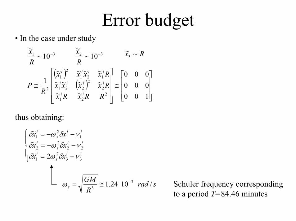
Error budget• In the case under study

31 10~~

−

Rx 32 10~

~−

Rx Rx ~~

3

( )( )

≅

≅100000000

~~~~~~~~~~

1

221

22

221

1212

1

2

RRxRxRxxxxRxxxx

RP

ii

iiii

iiii

thus obtaining:

−=−−=−−=

iis

i

iis

i

iis

i

xxxxxx

332

1

222

2

112

1

2 νδωδνδωδνδωδ

&&

&&

&&

sradR

GMs /1024.1 3

3−≅=ω Schuler frequency corresponding

to a period T=84.46 minutes

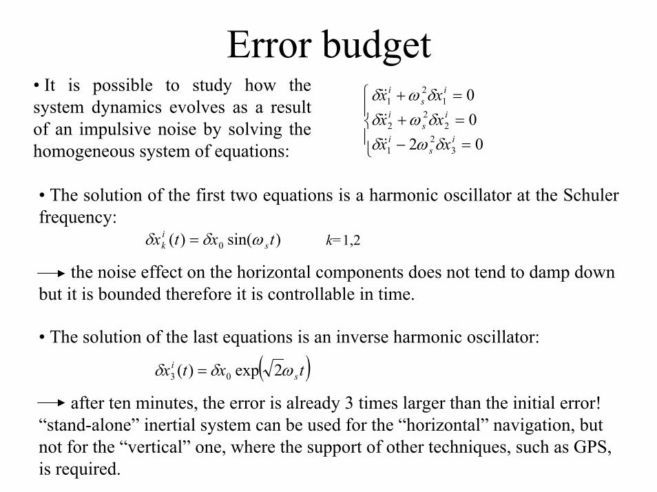
Error budget• It is possible to study how the system dynamics evolves as a result of an impulsive noise by solving the homogeneous system of equations:

=−=+=+

0200

32

1

22

2

12

1

is

i

is

i

is

i

xxxxxx

δωδδωδδωδ

&&

&&

&&

• The solution of the first two equations is a harmonic oscillator at the Schuler frequency:

)sin()( 0 txtx sik ωδδ = k=1,2

the noise effect on the horizontal components does not tend to damp down but it is bounded therefore it is controllable in time.

• The solution of the last equations is an inverse harmonic oscillator:

( )txtx si ωδδ 2exp)( 03 =

after ten minutes, the error is already 3 times larger than the initial error! “stand-alone” inertial system can be used for the “horizontal” navigation, but not for the “vertical” one, where the support of other techniques, such as GPS, is required.