Embed Size (px)
Citation preview
VALLURUPALLI NAGESWARA RAO VIGNANA JYOTHI INSTITUTE OF ENGINEERING & TECHNOLOGY
AN AUTONOMOUS INSTITUTE
(Approved by AICTE - New Delhi, Govt. of A.P.)
Accredited by NBA and NAAC with ‘A’ Grade
Vignana Jyothi Nagar, Bachupally, Nizampet (S.O.), Hyderabad-500 090. A.P., India.
ACADEMIC HAND BOOK
2017-2018
IV– B. TECH EEE
I SEMESTER
VNR VIGNANA JYOTHI INSTITUTE OF ENGINEERING AND TECHNOLOGY
AN AUTONOMOUS INSTITUTE
VISION
A Deemed University of Academic Excellence, for National and International Students
Meeting global Standards with social commitment and Democratic Values
MISSION
To produce global citizens with knowledge and commitment to strive to enhance quality of
life through meeting technological, educational, managerial and social challenges
QUALITY POLICY
• Impart up to date knowledge in the students chosen fields to make them quality Engineers
• Make the students experience the applications on quality equipment and tools.
• Provide quality environment and services to all stock holders.
• Provide Systems, resources and opportunities for continuous improvement.
• Maintain global standards in education, training, and services

VNR VIGNANA JYOTHI INSTITUTE OF ENGINEERING AND TECHNOLOGY
BACHUPALLY, NIZAMPET (S.O), HYDERABAD – 500090
LESSON PLAN: 2017-18
IV B. Tech : I Sem : EEE-1 L T/P/D C
3 0 3
Course Name: High Voltage Engineering Course Code:
13EEE017
Names of the Faculty Member: G.Radhika
Number of working days: 90
Number of Hours/week: 5
Total number of periods planned: 64
1. PREREQUISITES
13MTH001, 13MTH002, 13MTH005, 13PHY003, 13EEE001, 13ECE001, 13EEE101, 13ECE101
2. COURSE OBJECTIVES
The student should be able
• To review the concept of dielectrics and their behavior under a High Voltage
• To analyze methods for generation of High A.C, D.C & Impulse Voltages required for various application.
• To appraise the measuring techniques of High A.C., D.C & Impulse voltages and currents.
• To impart the knowledge of testing techniques for High Voltage Equipment.
3. COURSE OUTCOMES (COs)
Upon completion of this course the student is able to
1. Understand the applications of solid, liquid and gaseous dielectrics in electrical engineering.
2. Analyze the types of generation of High A.C, D.C & Impulse Voltages existing in research centers all over the world.
3. Interpret the necessity to measure the voltages and currents accurately, ensuring perfect safety to the personnel and
equipment.
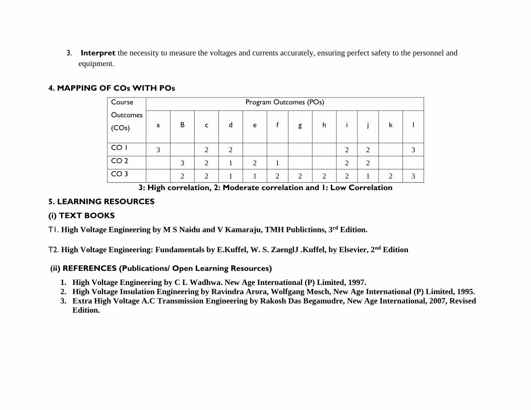
4. MAPPING OF COs WITH POs
Course
Outcomes
(COs)
Program Outcomes (POs)
a B c d e f g h i j k l
CO 1 3
2 2
2 2
3
CO 2
3 2 1 2 1
2 2
CO 3
2 2 1 1 2 2 2 2 1 2 3
3: High correlation, 2: Moderate correlation and 1: Low Correlation
5. LEARNING RESOURCES
(i) TEXT BOOKS
T1. High Voltage Engineering by M S Naidu and V Kamaraju, TMH Publictions, 3rd Edition.
T2. High Voltage Engineering: Fundamentals by E.Kuffel, W. S. ZaenglJ .Kuffel, by Elsevier, 2nd Edition
(ii) REFERENCES (Publications/ Open Learning Resources)
1. High Voltage Engineering by C L Wadhwa. New Age International (P) Limited, 1997.
2. High Voltage Insulation Engineering by Ravindra Arora, Wolfgang Mosch, New Age International (P) Limited, 1995.
3. Extra High Voltage A.C Transmission Engineering by Rakosh Das Begamudre, New Age International, 2007, Revised
Edition.
(a) Publications
[1] E. Kuffel, W.S. Zaengl and J. Kuffel, “High Voltage Engineering”, published by Butterworth Heinemann, 2000.
[2] S.M. Korobeynikov, Yu.N.Sinikh, “Bubbles and Breakdown of Liquid Dielectrics”, IEEE International Symposium on Electrical
Insulation, Arlington, Virginia, USA, June 7-10, 1998.
[3] S.S.Mohapatra, “High Voltage Engineering”, Dept. of Eee, S.I.E.T, Dhenkanal.
[4] Rastko Zivanovic, “High-Voltage Measurements”, Encyclopedia of Life Support Systems (EOLSS), Electrical Engineering – Vol.
II.
[5] A. P. (Sakis) Meliopoulos, “Lightning and Overvoltage Protection”, the McGraw-Hill Companies 2006.
(b) Open Learning Resources for self learning
L1. https://www.vidyarthiplus.com/vp/thread-6060.html#.WXcbm4SGPIV
L2. http://nptel.ac.in/courses/108104048/
L3: http://www.cpri.in/about-us/departmentsunits/high-voltage-division-hvd/hv-test-a-measurement-equipment.html
L4: http://www.meteorage.co.uk/meteorage/lightning-under-surveillance/the-lightning-phenomenon
(iii) JOURNALS
J1. IEEE Journal on Transmission & Distribution.
J2. IEEE Journal on Power Systems
J3. IEEMA Journal
6. DELIVERY METHODOLOGIES
DM1: Chalk and Talk DM5: Open The Box
DM3: Collaborative Learning (Think Pair Share, POGIL, etc.) DM7: Group Project
DM4: Demonstration (Physical / Laboratory / Audio Visuals)
7. PROPOSED FIELD VISITS/ GUEST LECTURE BY INDUSTRY EXPERT
Guest Lecture: "Application of High Voltage Engineering in “ by Mr. G. Hemanth , Sr. Design Engineer from CPRI, Bangalore, is
scheduled on 14/09/2017.
(And / Or)
Field Visit: As a part of class, field visit is scheduled to CENTRAL POWER RESEARCH INSTITUTE, (UHVRL) RESEARCH LAB
on 22/09/2017.
8. ASSESSMENT
AM1: Semester End Examination . AM2: Mid Term Examination
AM3: Home Assignments
AM6: Quizzes
AM7: Course Projects**
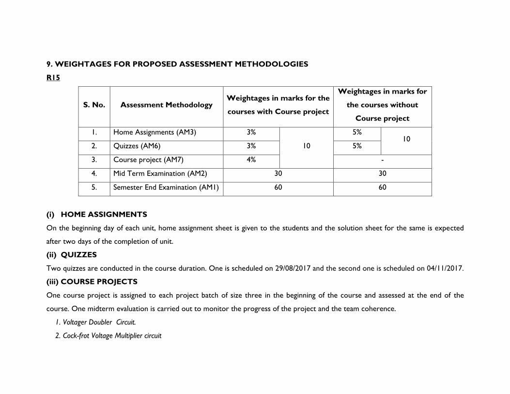
9. WEIGHTAGES FOR PROPOSED ASSESSMENT METHODOLOGIES
R15
S. No. Assessment Methodology Weightages in marks for the
courses with Course project
Weightages in marks for
the courses without
Course project
1. Home Assignments (AM3) 3%
10
5% 10
2. Quizzes (AM6) 3% 5%
3. Course project (AM7) 4% -
4. Mid Term Examination (AM2) 30 30
5. Semester End Examination (AM1) 60 60
(i) HOME ASSIGNMENTS
On the beginning day of each unit, home assignment sheet is given to the students and the solution sheet for the same is expected
after two days of the completion of unit.
(ii) QUIZZES
Two quizzes are conducted in the course duration. One is scheduled on 29/08/2017 and the second one is scheduled on 04/11/2017.
(iii) COURSE PROJECTS
One course project is assigned to each project batch of size three in the beginning of the course and assessed at the end of the
course. One midterm evaluation is carried out to monitor the progress of the project and the team coherence.
1. Voltager Doubler Circuit.
2. Cock-frot Voltage Multiplier circuit
3. Tesla Coil
4. Impulse Voltage Generator
5. Impulse Current Generator
10. SIMULATION SOFTWARES (If any)
1. PSpice
2. PSIM power electronics simulator
3. MATLAB
4. PSCAD/EMTDC
11. DETAILED COURSE DELIVERY PLAN
UNIT I
INTRODUCTION TO HIGH VOLTAGE TECHNOLOGY AND APPLICATIONS: Electric Field, Stresses, Gas / Vacuum as
Insulator, Liquid Dielectrics, Solids and Composites, Estimation and Control of Electric Stress, Numerical methods for electric field
computation, Surge voltages, their distribution and Control, Applications of insulating materials in transformers, rotating machines,
circuit breakers, cable power capacitors and bushings.
Learning Outcomes
On the conclusion of the Unit –I, the student must be able to understand
• Difference types of insulating medium and their applications.
Electric field stresses and numerical approach for computation
UNIT II
BREAK DOWN IN GASEOUS AND LIQUID DIELECTRICS: Gases as insulating media, collision process, Ionization process,
Townsend’s criteria of breakdown in gases, Paschen’s law. Liquid as Insulator, pure and commercial liquids, breakdown in pure and
commercial liquids.
Intrinsic breakdown, electromechanical breakdown, thermal breakdown, breakdown of solid dielectrics in practice, Breakdown in
composite dielectrics, solid dielectrics used in practice.
Learning Objectives:
On the conclusion of the Unit –II, the student must be able to understand
• Working of gases and liquid dielectrics.
• Different criterion for breakdown of dielectrics.
• Solid dielectrics and their breakdown phenomenon.
UNIT III
GENERATION OF HIGH VOLTAGES AND CURRENTS: Generation of High Direct Current Voltages, Generation of High
alternating voltages, Generation of Impulse Voltages, Generation of Impulse currents, Tripping and control of impulse generators.
Learning Objectives:
On the conclusion of the Unit –IV, the student must be able to understand
• Different methods to generate dc, ac and impulse voltages and currents.
UNIT IV
MEASUREMENT OF HIGH VOLTAGES AND CURRENTS: Measurement of High Direct Current Voltages, Measurement of
High Voltages alternating and impulse, Measurement of High Currents-direct, alternating and Impulse, Oscilloscope for impulse
voltage and current measurements. Measurement of D.C Resistivity, Measurement of Dielectric Constant and loss factor, Partial
discharge measurements.
Learning Objectives:
On the conclusion of the Unit –V, the student must be able to understand
• Different methods to measure dc, ac and impulse voltages and currents.
• How to determine DC resistivity, dielectric constant and loss factor.
UNIT V
OVER VOLTAGE PHENOMENON AND INSULATION CO-ORDINATION: Natural causes for over voltages – Lightning
phenomenon, Over voltage due to switching surges, system faults and other abnormal conditions, Principles of Insulation
Coordination on High voltage and Extra High Voltage power systems. Testing of Insulators and bushings, Testing of Isolators and
circuit breakers, Testing of cables, Testing of Transformers, Testing of Surge Arresters, Radio Interference measurements.
Learning Objectives:
On the conclusion of the Unit –VI, the student must be able to understand
• Different types of over voltages and their causes.
• Insulation coordination on power systems.
• Testing methods for high voltage equipments.
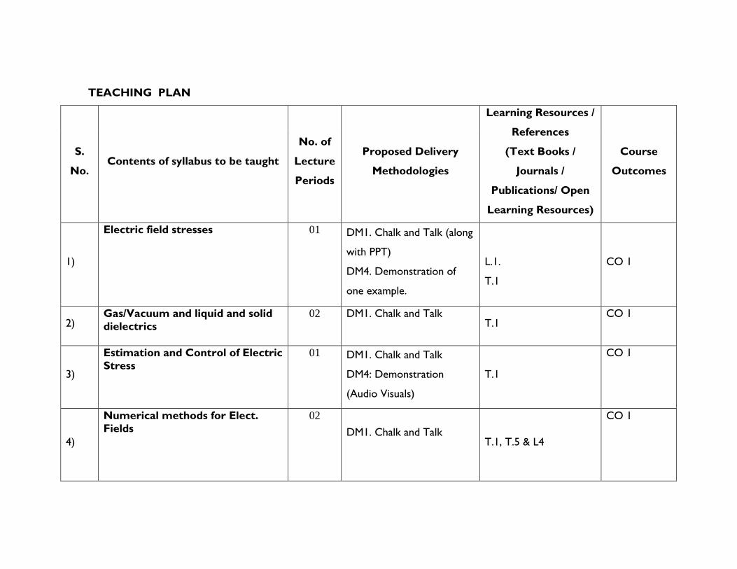
TEACHING PLAN
S.
No. Contents of syllabus to be taught
No. of
Lecture
Periods
Proposed Delivery
Methodologies
Learning Resources /
References
(Text Books /
Journals /
Publications/ Open
Learning Resources)
Course
Outcomes
1)
Electric field stresses 01 DM1. Chalk and Talk (along
with PPT)
DM4. Demonstration of
one example.
L.1.
T.1
CO 1
2) Gas/Vacuum and liquid and solid
dielectrics
02 DM1. Chalk and Talk
T.1
CO 1
3)
Estimation and Control of Electric
Stress
01 DM1. Chalk and Talk
DM4: Demonstration
(Audio Visuals)
T.1
CO 1
4)
Numerical methods for Elect.
Fields
02
DM1. Chalk and Talk
T.1, T.5 & L4
CO 1
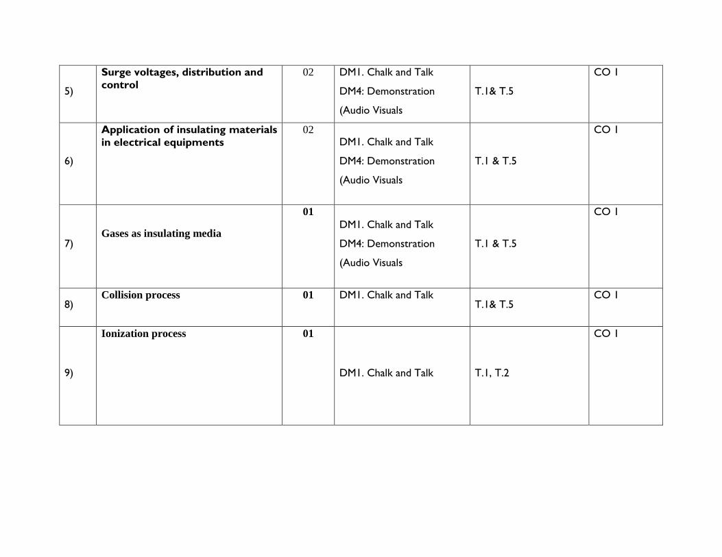
5)
Surge voltages, distribution and
control
02 DM1. Chalk and Talk
DM4: Demonstration
(Audio Visuals
T.1& T.5
CO 1
6)
Application of insulating materials
in electrical equipments
02 DM1. Chalk and Talk
DM4: Demonstration
(Audio Visuals
T.1 & T.5
CO 1
7)
Gases as insulating media
01
DM1. Chalk and Talk
DM4: Demonstration
(Audio Visuals
T.1 & T.5
CO 1
8) Collision process 01 DM1. Chalk and Talk
T.1& T.5
CO 1
9)
Ionization process 01
DM1. Chalk and Talk T.1, T.2
CO 1
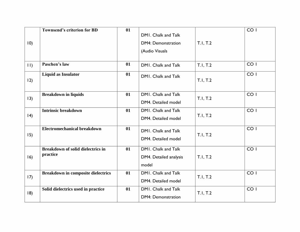
10)
Townsend’s criterion for BD 01
DM1. Chalk and Talk
DM4: Demonstration
(Audio Visuals
T.1, T.2
CO 1
11) Paschen’s law 01 DM1. Chalk and Talk T.1, T.2 CO 1
12)
Liquid as Insulator 01 DM1. Chalk and Talk
T.1, T.2
CO 1
13) Breakdown in liquids 01 DM1. Chalk and Talk
DM4. Detailed model T.1, T.2
CO 1
14) Intrinsic breakdown
01 DM1. Chalk and Talk
DM4. Detailed model T.1, T.2
CO 1
15)
Electromechanical breakdown 01 DM1. Chalk and Talk
DM4. Detailed model T.1, T.2
CO 1
16)
Breakdown of solid dielectrics in
practice
01 DM1. Chalk and Talk
DM4. Detailed analysis
model
T.1, T.2
CO 1
17) Breakdown in composite dielectrics 01 DM1. Chalk and Talk
DM4. Detailed model T.1, T.2
CO 1
18) Solid dielectrics used in practice 01 DM1. Chalk and Talk
DM4: Demonstration T.1, T.2
CO 1
(Audio Visuals)
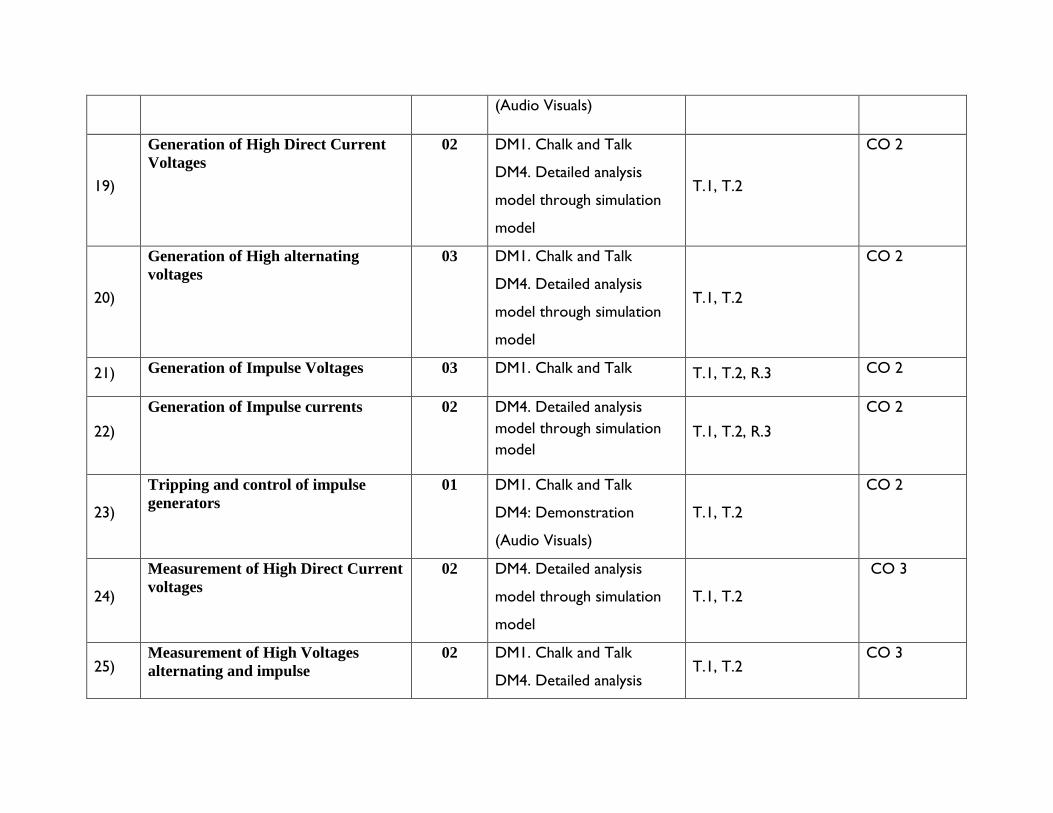
19)
Generation of High Direct Current
Voltages
02 DM1. Chalk and Talk
DM4. Detailed analysis
model through simulation
model
T.1, T.2
CO 2
20)
Generation of High alternating
voltages
03 DM1. Chalk and Talk
DM4. Detailed analysis
model through simulation
model
T.1, T.2
CO 2
21) Generation of Impulse Voltages 03 DM1. Chalk and Talk T.1, T.2, R.3 CO 2
22)
Generation of Impulse currents 02 DM4. Detailed analysis
model through simulation
model T.1, T.2, R.3
CO 2
23)
Tripping and control of impulse
generators
01 DM1. Chalk and Talk
DM4: Demonstration
(Audio Visuals)
T.1, T.2
CO 2
24)
Measurement of High Direct Current
voltages
02 DM4. Detailed analysis
model through simulation
model
T.1, T.2
CO 3
25) Measurement of High Voltages
alternating and impulse
02 DM1. Chalk and Talk
DM4. Detailed analysis T.1, T.2
CO 3

model
26)
Measurement of High direct
Currents
02 DM1. Chalk and Talk
DM4. Detailed analysis
model
T.1, T.2
CO 3
27)
Measurement of High alternating
Currents
02 DM1. Chalk and Talk
DM4. Detailed analysis
model
T.1, T.2
CO 3
28)
Measurement of High impulse
Currents
01 DM1. Chalk and Talk
DM4. Detailed analysis
model
T.1, T.2
CO 3
29)
Measurement of D.C Resistivity 01 DM1. Chalk and Talk
DM4. Detailed analysis
model
T.1, T.2
CO 3
30)
Measurement of D.C Resistivity 01 DM1. Chalk and Talk
DM4. Detailed analysis
model
T.1, T.2
CO 3
31)
Partial discharge measurements 01 DM1. Chalk and Talk
DM4. Detailed analysis
model
T.1, T.2
CO 4
32) Numerical Problems 04 DM1. Chalk and Talk
T.1, T.2
CO 4
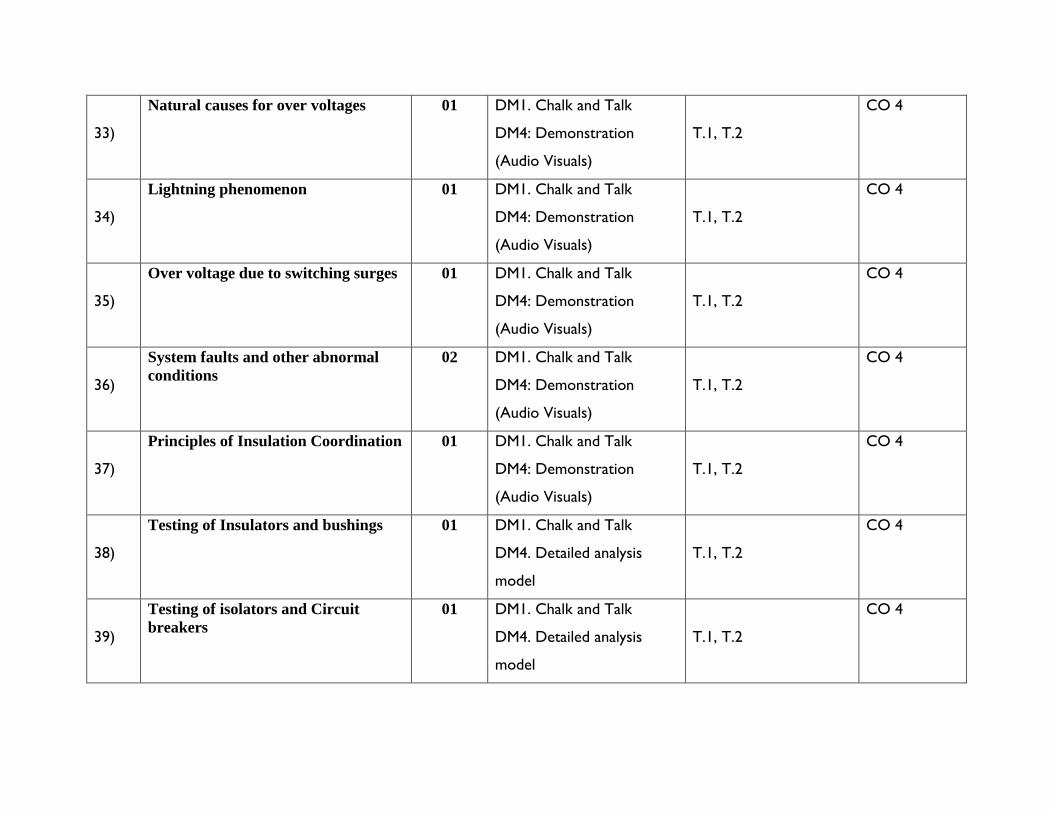
33)
Natural causes for over voltages 01 DM1. Chalk and Talk
DM4: Demonstration
(Audio Visuals)
T.1, T.2
CO 4
34)
Lightning phenomenon 01 DM1. Chalk and Talk
DM4: Demonstration
(Audio Visuals)
T.1, T.2
CO 4
35)
Over voltage due to switching surges 01 DM1. Chalk and Talk
DM4: Demonstration
(Audio Visuals)
T.1, T.2
CO 4
36)
System faults and other abnormal
conditions
02 DM1. Chalk and Talk
DM4: Demonstration
(Audio Visuals)
T.1, T.2
CO 4
37)
Principles of Insulation Coordination 01 DM1. Chalk and Talk
DM4: Demonstration
(Audio Visuals)
T.1, T.2
CO 4
38)
Testing of Insulators and bushings 01 DM1. Chalk and Talk
DM4. Detailed analysis
model
T.1, T.2
CO 4
39)
Testing of isolators and Circuit
breakers
01 DM1. Chalk and Talk
DM4. Detailed analysis
model
T.1, T.2
CO 4
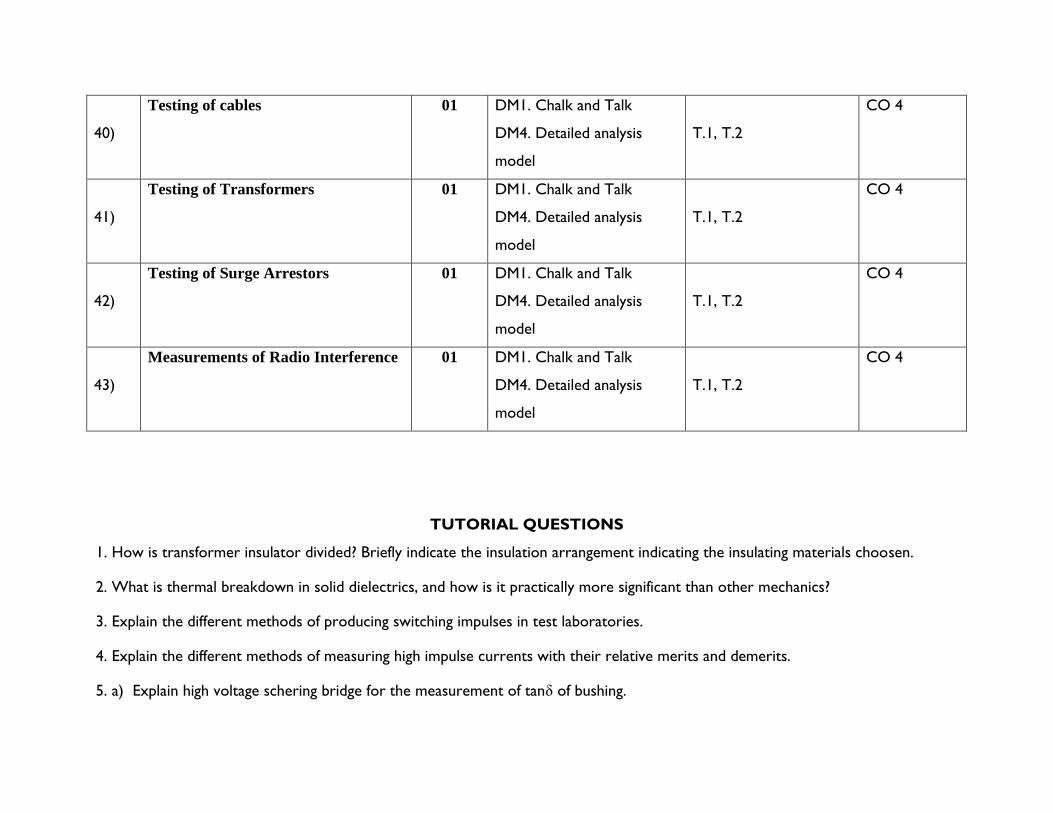
40)
Testing of cables 01 DM1. Chalk and Talk
DM4. Detailed analysis
model
T.1, T.2
CO 4
41)
Testing of Transformers 01 DM1. Chalk and Talk
DM4. Detailed analysis
model
T.1, T.2
CO 4
42)
Testing of Surge Arrestors 01 DM1. Chalk and Talk
DM4. Detailed analysis
model
T.1, T.2
CO 4
43)
Measurements of Radio Interference 01 DM1. Chalk and Talk
DM4. Detailed analysis
model
T.1, T.2
CO 4
TUTORIAL QUESTIONS
1. How is transformer insulator divided? Briefly indicate the insulation arrangement indicating the insulating materials choosen.
2. What is thermal breakdown in solid dielectrics, and how is it practically more significant than other mechanics?
3. Explain the different methods of producing switching impulses in test laboratories.
4. Explain the different methods of measuring high impulse currents with their relative merits and demerits.
5. a) Explain high voltage schering bridge for the measurement of tanδ of bushing.
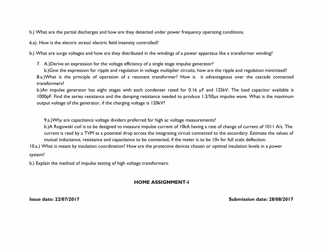
b.) What are the partial discharges and how are they detected under power frequency operating conditions.
6.a). How is the electric stress/ electric field intensity controlled?
b.) What are surge voltages and how are they distributed in the windings of a power apparatus like a transformer winding?
7. A.)Derive an expression for the voltage efficiency of a single stage impulse generator?
b.)Give the expression for ripple and regulation in voltage multiplier circuits, how are the ripple and regulation minimized?
8.a.)What is the principle of operation of a resonant transformer? How is it advantageous over the cascade connected
transformers?
b.)An impulse generator has eight stages with each condenser rated for 0.16 µF and 125kV. The load capacitor available is
1000pF. Find the series resistance and the damping resistance needed to produce 1.2/50µs impulse wave. What is the maximum
output voltage of the generator, if the charging voltage is 120kV?
9.a.)Why are capacitance voltage dividers preferred for high ac voltage measurements?
b.)A Rogowski coil is to be designed to measure impulse current of 10kA having a rate of change of current of 1011 A/s. The
current is read by a TVM as a potential drop across the integrating circuit connected to the secondary. Estimate the values of
mutual inductance, resistance and capacitance to be connected, if the meter is to be 10v for full scale deflection.
10.a.) What is meant by insulation coordination? How are the protective devices chosen or optimal insulation levels in a power
system?
b.) Explain the method of impulse testing of high voltage transformers.
HOME ASSIGNMENT-I
Issue date: 22/07/2017 Submission date: 28/08/2017
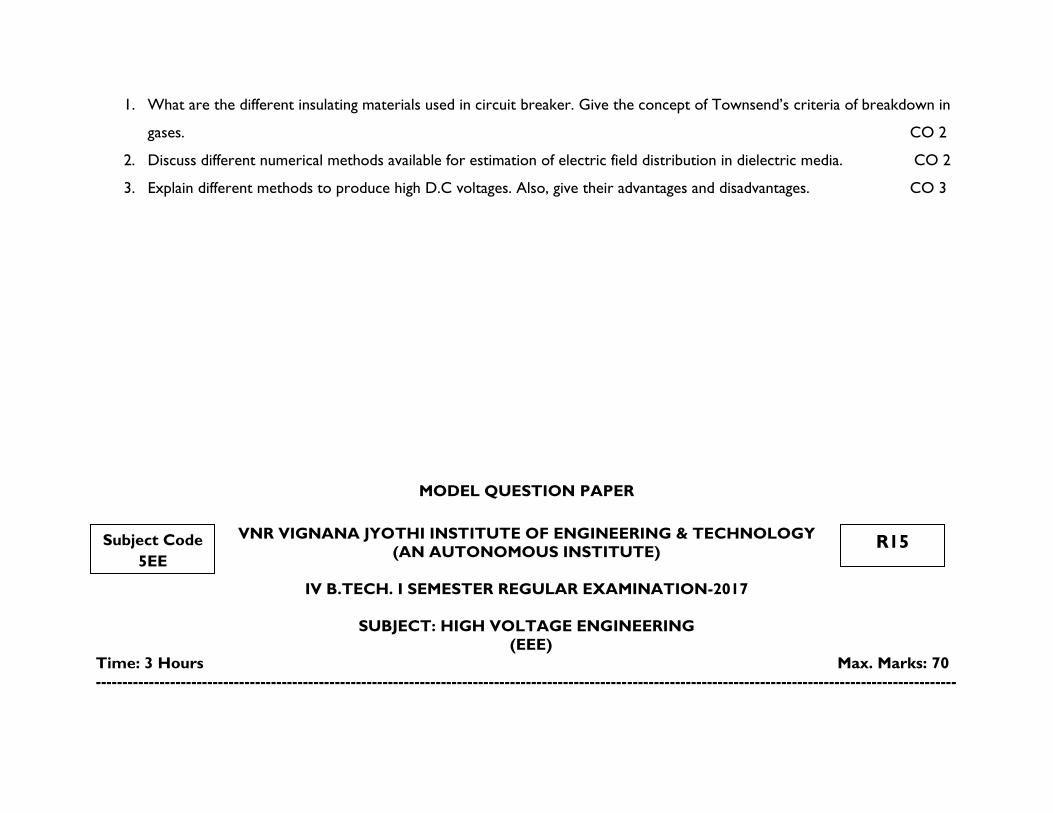
1. What are the different insulating materials used in circuit breaker. Give the concept of Townsend’s criteria of breakdown in
gases. CO 2
2. Discuss different numerical methods available for estimation of electric field distribution in dielectric media. CO 2
3. Explain different methods to produce high D.C voltages. Also, give their advantages and disadvantages. CO 3
MODEL QUESTION PAPER
VNR VIGNANA JYOTHI INSTITUTE OF ENGINEERING & TECHNOLOGY
(AN AUTONOMOUS INSTITUTE)
IV B.TECH. I SEMESTER REGULAR EXAMINATION-2017
SUBJECT: HIGH VOLTAGE ENGINEERING
(EEE)
Time: 3 Hours Max. Marks: 70
------------------------------------------------------------------------------------------------------------------------------------------------------------------
Subject Code
5EE
R15

Part - A
1. Answer in one sentence 5X1=5M
a.) Define Paschen’s Law
b.) Define Partial Discharge?
c.) Define loss factor
d.) List out the different types of cables.
e.) What are surge arresters
2. Answer the following briefly 5X2=10M
a.) Discuss briefly about electric field stresses.
b.) What is ionization process?
c.) Name the instruments for measurement of high DC voltages?
d.) What is impulse voltage?
e.) What is insulation coordination?
3. Answer the following very briefly 5X3=15M
a.) Explain about thermal breakdown in solid dielectrics.
b.) Explain measurement of DC resistivity
c.) Explain in detail about the generation of impulse currents.
d.) Explain the application of insulating materials in transformers.
e.) Give an account of different tests performed on cables?
Part - B
Answer any Four questions 4X10=40M
4. a.) Explain in detail about applications of insulating material in rotating machines
b.) Explain about estimation and control of Electric stress.
5. a.) Explain in detail about the electromechanical breakdown.
b.) What are pure and commercial liquids.
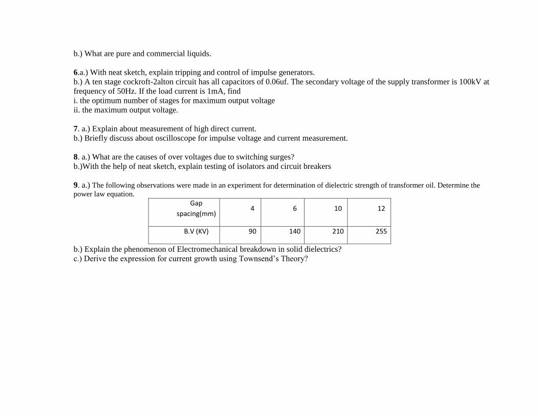
6.a.) With neat sketch, explain tripping and control of impulse generators.
b.) A ten stage cockroft-2alton circuit has all capacitors of 0.06uf. The secondary voltage of the supply transformer is 100kV at
frequency of 50Hz. If the load current is 1mA, find
i. the optimum number of stages for maximum output voltage
ii. the maximum output voltage.
7. a.) Explain about measurement of high direct current.
b.) Briefly discuss about oscilloscope for impulse voltage and current measurement.
8. a.) What are the causes of over voltages due to switching surges?
b.)With the help of neat sketch, explain testing of isolators and circuit breakers
9. a.) The following observations were made in an experiment for determination of dielectric strength of transformer oil. Determine the
power law equation.
Gap
spacing(mm) 4 6 10 12
B.V (KV) 90 140 210 255
b.) Explain the phenomenon of Electromechanical breakdown in solid dielectrics?
c.) Derive the expression for current growth using Townsend’s Theory?
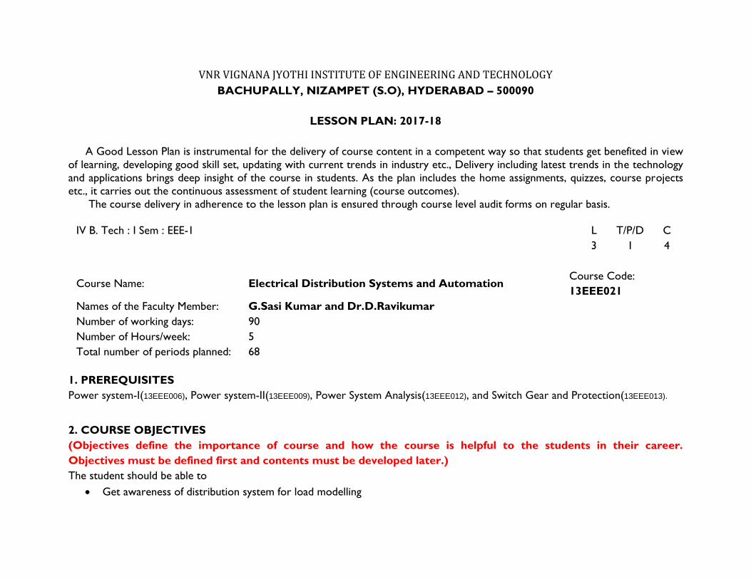
VNR VIGNANA JYOTHI INSTITUTE OF ENGINEERING AND TECHNOLOGY
BACHUPALLY, NIZAMPET (S.O), HYDERABAD – 500090
LESSON PLAN: 2017-18
A Good Lesson Plan is instrumental for the delivery of course content in a competent way so that students get benefited in view
of learning, developing good skill set, updating with current trends in industry etc., Delivery including latest trends in the technology
and applications brings deep insight of the course in students. As the plan includes the home assignments, quizzes, course projects
etc., it carries out the continuous assessment of student learning (course outcomes).
The course delivery in adherence to the lesson plan is ensured through course level audit forms on regular basis.
IV B. Tech : I Sem : EEE-1 L T/P/D C
3 1 4
Course Name: Electrical Distribution Systems and Automation Course Code:
13EEE021
Names of the Faculty Member: G.Sasi Kumar and Dr.D.Ravikumar
Number of working days: 90
Number of Hours/week: 5
Total number of periods planned: 68
1. PREREQUISITES
Power system-I(13EEE006), Power system-II(13EEE009), Power System Analysis(13EEE012), and Switch Gear and Protection(13EEE013).
2. COURSE OBJECTIVES
(Objectives define the importance of course and how the course is helpful to the students in their career.
Objectives must be defined first and contents must be developed later.)
The student should be able to
• Get awareness of distribution system for load modelling
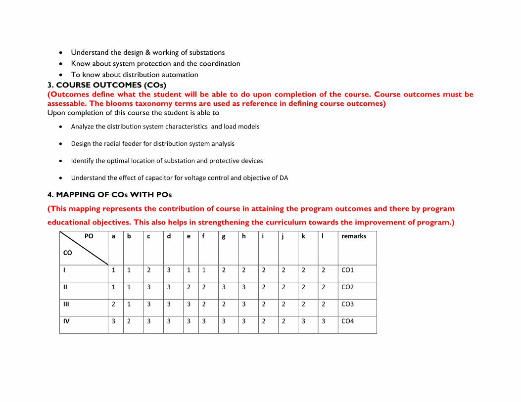
• Understand the design & working of substations
• Know about system protection and the coordination
• To know about distribution automation
3. COURSE OUTCOMES (COs)
(Outcomes define what the student will be able to do upon completion of the course. Course outcomes must be
assessable. The blooms taxonomy terms are used as reference in defining course outcomes)
Upon completion of this course the student is able to
• Analyze the distribution system characteristics and load models
• Design the radial feeder for distribution system analysis
• Identify the optimal location of substation and protective devices
• Understand the effect of capacitor for voltage control and objective of DA
4. MAPPING OF COs WITH POs
(This mapping represents the contribution of course in attaining the program outcomes and there by program
educational objectives. This also helps in strengthening the curriculum towards the improvement of program.)
PO
CO
a b c d e f g h i j k l remarks
I 1 1 2 3 1 1 2 2 2 2 2 2 CO1
II 1 1 3 3 2 2 3 3 2 2 2 2 CO2
III 2 1 3 3 3 2 2 3 2 2 2 2 CO3
IV 3 2 3 3 3 3 3 3 2 2 3 3 CO4
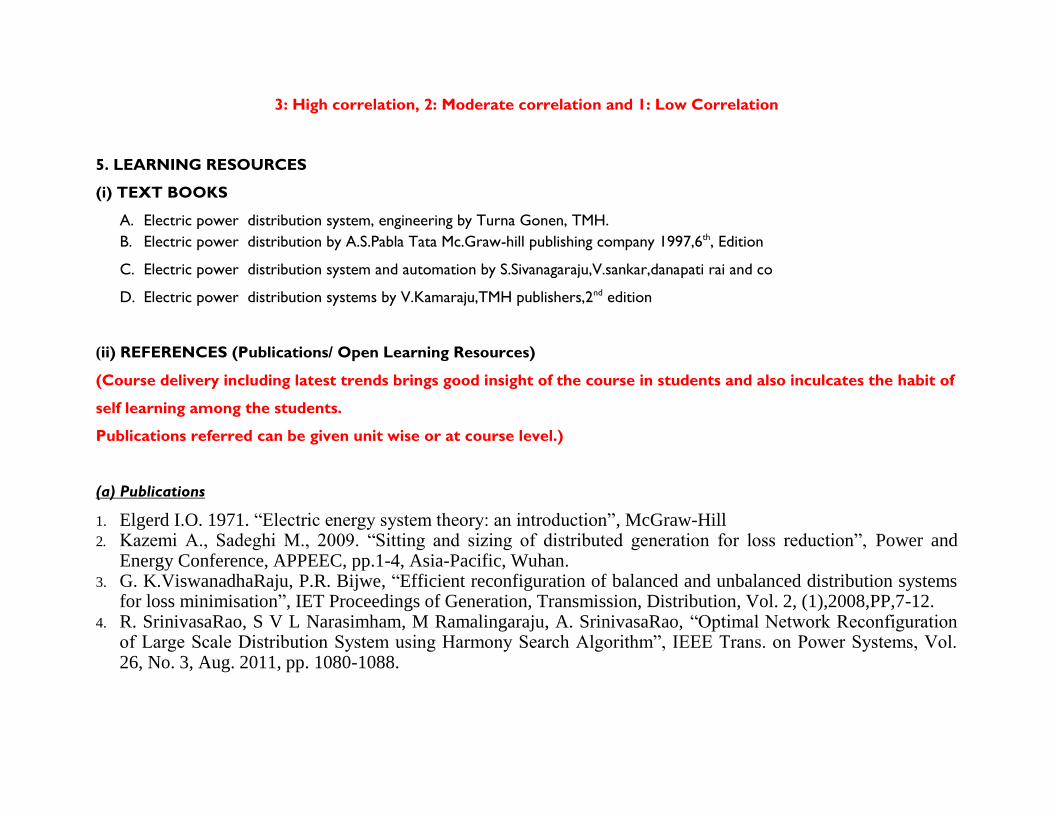
3: High correlation, 2: Moderate correlation and 1: Low Correlation
5. LEARNING RESOURCES
(i) TEXT BOOKS
A. Electric power distribution system, engineering by Turna Gonen, TMH.
B. Electric power distribution by A.S.Pabla Tata Mc.Graw-hill publishing company 1997,6th, Edition
C. Electric power distribution system and automation by S.Sivanagaraju,V.sankar,danapati rai and co
D. Electric power distribution systems by V.Kamaraju,TMH publishers,2nd edition
(ii) REFERENCES (Publications/ Open Learning Resources)
(Course delivery including latest trends brings good insight of the course in students and also inculcates the habit of
self learning among the students.
Publications referred can be given unit wise or at course level.)
(a) Publications
1. Elgerd I.O. 1971. “Electric energy system theory: an introduction”, McGraw-Hill 2. Kazemi A., Sadeghi M., 2009. “Sitting and sizing of distributed generation for loss reduction”, Power and
Energy Conference, APPEEC, pp.1-4, Asia-Pacific, Wuhan. 3. G. K.ViswanadhaRaju, P.R. Bijwe, “Efficient reconfiguration of balanced and unbalanced distribution systems
for loss minimisation”, IET Proceedings of Generation, Transmission, Distribution, Vol. 2, (1),2008,PP,7-12. 4. R. SrinivasaRao, S V L Narasimham, M Ramalingaraju, A. SrinivasaRao, “Optimal Network Reconfiguration
of Large Scale Distribution System using Harmony Search Algorithm”, IEEE Trans. on Power Systems, Vol. 26, No. 3, Aug. 2011, pp. 1080-1088.
(b) Open Learning Resources for self learning
L1 http://nptel.ac.in/courses/108102047/23 distribution system
L2 http://nptel.ac.in/courses/108102047/31 (CONTROL OF VOLTAGE)
L3 http://nptel.ac.in/courses/108102047/13 methods of voltage control
L4 http://pages.mtu.edu/~avsergue/EET3390/Lectures/CHAPTER6.pdf substation
L5 http://nptel.ac.in/ (Feeder voltage regulation)
L6 https://www.youtube.com/watch?v=zCiPlEBolsI
(iii) JOURNALS
J1. IEEE Journal on Power systems
J2. IEEE Journal on Power delivery.
J3. IEEE Journal on Power and Energy.
J4. IEEE Transactions on Power systems.
6. DELIVERY METHODOLOGIES
(Depending on the suitability to the delivery of concept, one or more among the following delivery methodologies
are adopted to engage the student in learning)
DM1: Chalk and Talk DM5: Open The Box
DM3: Collaborative Learning (Think Pair Share, POGIL, etc.) DM7: Group Project
DM4: Demonstration (Physical / Laboratory / Audio Visuals)
7. PROPOSED FIELD VISITS/ GUEST LECTURE BY INDUSTRY EXPERT
(To be added for the courses as directed by the department.)
Guest Lecture: "topic of Losses reduction in power Distribution system " by Mr. X Engineer from Y industry is scheduled on
24/09/2017
(And / Or)
Field Visit: As a part of class, field visit is scheduled to substation industry on 22/10/2017.
8. ASSESSMENT
(As per Regulations, AM1 and AM2 are compulsory for assessment. Whereas, any two or more assessment
methodologies can be considered from AM3 to AM9 under assignment towards continuous assessment of the
performance of students.)
AM1: Semester End Examination . AM2: Mid Term Examination
AM3: Home Assignments AM6: Quizzes
AM7: Course Projects**
** (To be added for the courses as directed by the department. The no. of course projects is left to the liberty of
faculty)
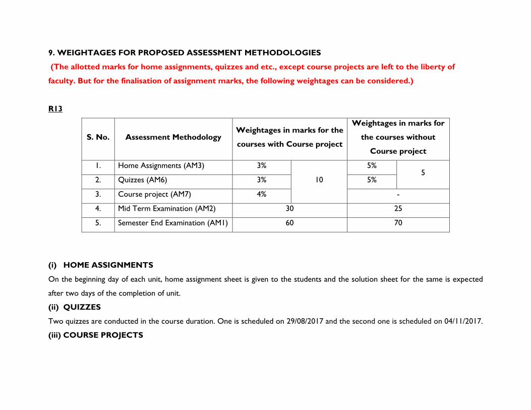
9. WEIGHTAGES FOR PROPOSED ASSESSMENT METHODOLOGIES
(The allotted marks for home assignments, quizzes and etc., except course projects are left to the liberty of
faculty. But for the finalisation of assignment marks, the following weightages can be considered.)
R13
S. No. Assessment Methodology Weightages in marks for the
courses with Course project
Weightages in marks for
the courses without
Course project
1. Home Assignments (AM3) 3%
10
5% 5
2. Quizzes (AM6) 3% 5%
3. Course project (AM7) 4% -
4. Mid Term Examination (AM2) 30 25
5. Semester End Examination (AM1) 60 70
(i) HOME ASSIGNMENTS
On the beginning day of each unit, home assignment sheet is given to the students and the solution sheet for the same is expected
after two days of the completion of unit.
(ii) QUIZZES
Two quizzes are conducted in the course duration. One is scheduled on 29/08/2017 and the second one is scheduled on 04/11/2017.
(iii) COURSE PROJECTS
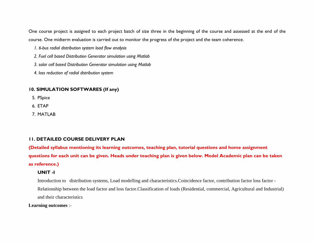
One course project is assigned to each project batch of size three in the beginning of the course and assessed at the end of the
course. One midterm evaluation is carried out to monitor the progress of the project and the team coherence.
1. 6-bus radial distribution system load flow analysis
2. Fuel cell based Distribution Generator simulation using Matlab
3. solar cell based Distribution Generator simulation using Matlab
4. loss reduction of radial distribution system
10. SIMULATION SOFTWARES (If any)
5. PSpice
6. ETAP
7. MATLAB
11. DETAILED COURSE DELIVERY PLAN
(Detailed syllabus mentioning its learning outcomes, teaching plan, tutorial questions and home assignment
questions for each unit can be given. Heads under teaching plan is given below. Model Academic plan can be taken
as reference.)
UNIT -I
Introduction to distribution systems, Load modelling and characteristics.Coincidence factor, contribution factor loss factor -
Relationship between the load factor and loss factor.Classification of loads (Residential, commercial, Agricultural and Industrial)
and their characteristics
Learning outcomes :-
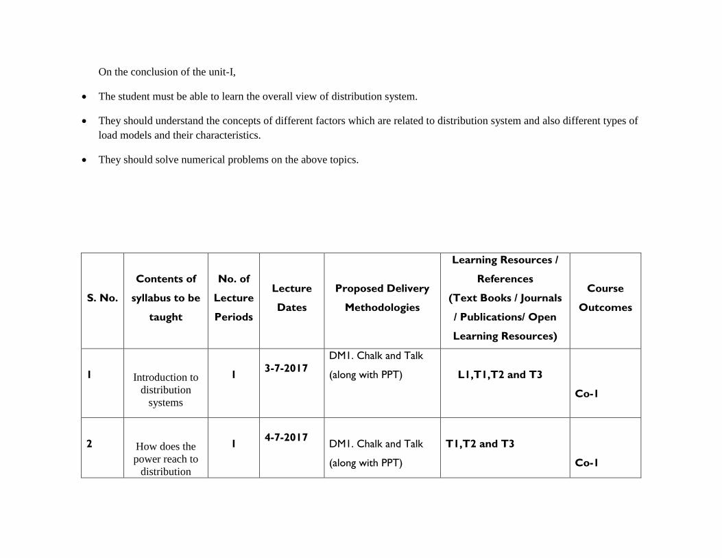
On the conclusion of the unit-I,
• The student must be able to learn the overall view of distribution system.
• They should understand the concepts of different factors which are related to distribution system and also different types of
load models and their characteristics.
• They should solve numerical problems on the above topics.
S. No.
Contents of
syllabus to be
taught
No. of
Lecture
Periods
Lecture
Dates
Proposed Delivery
Methodologies
Learning Resources /
References
(Text Books / Journals
/ Publications/ Open
Learning Resources)
Course
Outcomes
1
Introduction to
distribution
systems
1
3-7-2017
DM1. Chalk and Talk
(along with PPT)
L1,T1,T2 and T3
Co-1
2
How does the
power reach to
distribution
1
4-7-2017
DM1. Chalk and Talk
(along with PPT)
T1,T2 and T3
Co-1
system
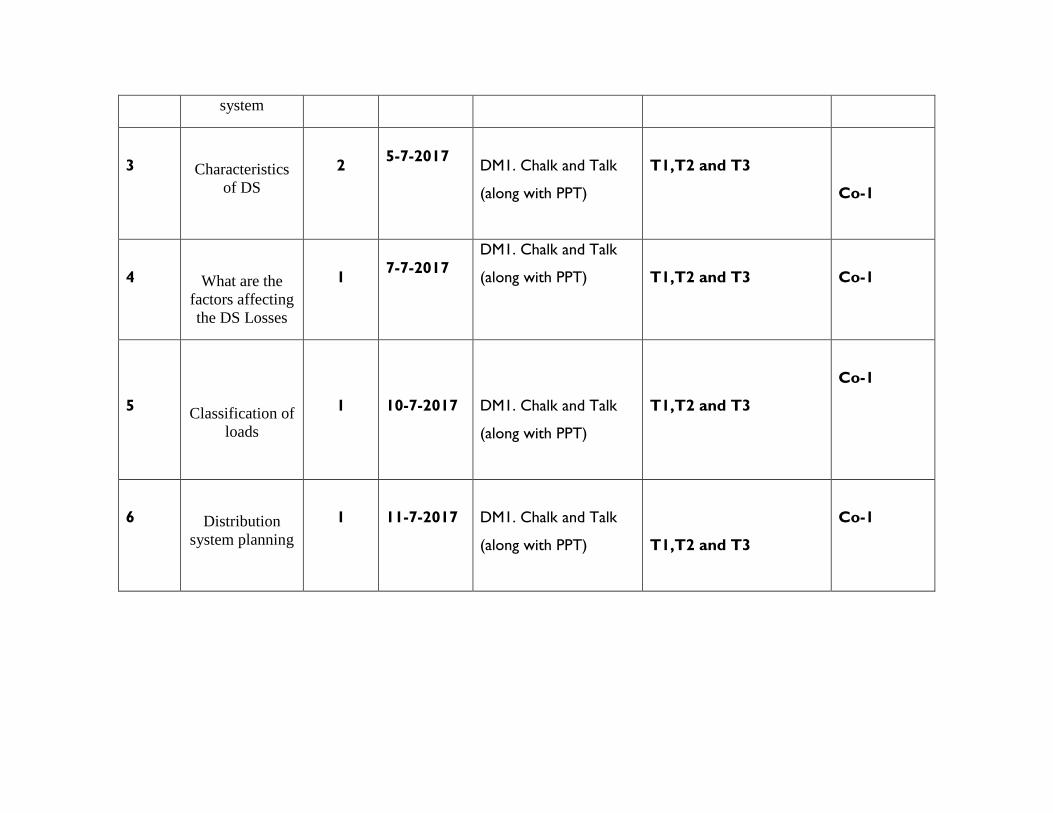
3
Characteristics
of DS
2
5-7-2017
DM1. Chalk and Talk
(along with PPT)
T1,T2 and T3
Co-1
4
What are the
factors affecting
the DS Losses
1
7-7-2017
DM1. Chalk and Talk
(along with PPT)
T1,T2 and T3
Co-1
5
Classification of
loads
1
10-7-2017
DM1. Chalk and Talk
(along with PPT)
T1,T2 and T3
Co-1
6
Distribution
system planning
1
11-7-2017
DM1. Chalk and Talk
(along with PPT)
T1,T2 and T3
Co-1
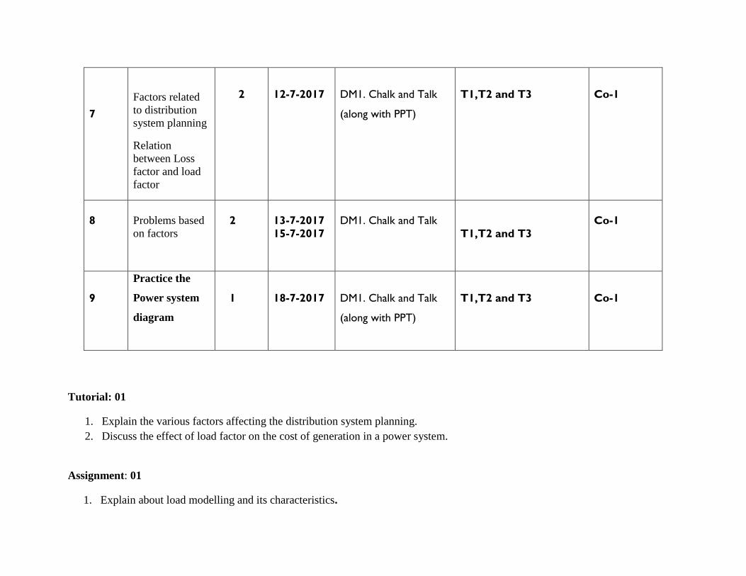
7
Factors related
to distribution
system planning
Relation
between Loss
factor and load
factor
2
12-7-2017
DM1. Chalk and Talk
(along with PPT)
T1,T2 and T3
Co-1
8
Problems based
on factors
2
13-7-2017
15-7-2017
DM1. Chalk and Talk
T1,T2 and T3
Co-1
9
Practice the
Power system
diagram
1
18-7-2017
DM1. Chalk and Talk
(along with PPT)
T1,T2 and T3
Co-1
Tutorial: 01
1. Explain the various factors affecting the distribution system planning.
2. Discuss the effect of load factor on the cost of generation in a power system.
Assignment: 01
1. Explain about load modelling and its characteristics.

2. Define the following terms with suitable examples.
i) Load factor ii) loss factor iii) contribution factor.
UNIT- II
Design Considerations of Distribution Feeders: Radial and loop types of primary feeders, voltage levels, feeder loading; basic design
practice of the secondary distribution system. Location of Substations: Rating of distribution substation, service area with in primary
feeders. Benefits derived through optimal location of substations.
Learning objectives:- (not required)
On the conclusion of the unit-II,
• The student must be able to learn the concept of various types of distribution feeders.
• Learn the concept of substations
• Learn benefits through optimal location of substations.
LEARNING OUTCOMES
After completion of this unit the student will be able to
1. Identify the distribution system for providing the reliable supply to end customers
2. Compare advantages and disadvantages among the primary distribution systems
3. Understand the Optimal location of substation

TEACHING PLAN
S.
No. Contents of syllabus to be taught
No. of
Lecture
Periods
Lecture
Dates
Proposed Delivery
Methodologies
Learning Resources /
References
(Text Books /
Course
Outcomes
Journals /
Publications/ Open
Learning Resources)
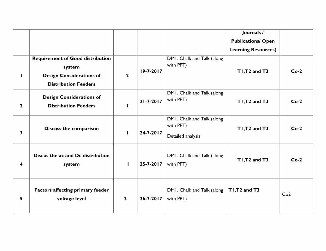
1
Requirement of Good distribution
system
Design Considerations of
Distribution Feeders
2
19-7-2017
DM1. Chalk and Talk (along
with PPT)
T1,T2 and T3 Co-2
2
Design Considerations of
Distribution Feeders
1
21-7-2017
DM1. Chalk and Talk (along
with PPT) T1,T2 and T3 Co-2
3
Discuss the comparison
1
24-7-2017
DM1. Chalk and Talk (along
with PPT)
Detailed analysis
T1,T2 and T3 Co-2
4
Discus the ac and Dc distribution
system
1
25-7-2017
DM1. Chalk and Talk (along
with PPT)
T1,T2 and T3 Co-2
5
Factors affecting primary feeder
voltage level
2
26-7-2017
DM1. Chalk and Talk (along
with PPT)
T1,T2 and T3
Co2
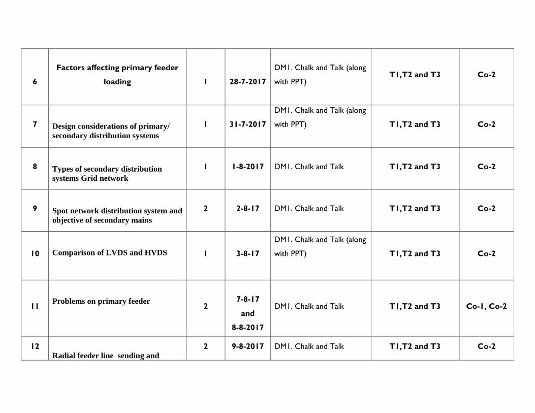
6
Factors affecting primary feeder
loading
1
28-7-2017
DM1. Chalk and Talk (along
with PPT)
T1,T2 and T3 Co-2
7
Design considerations of primary/
secondary distribution systems
1 31-7-2017
DM1. Chalk and Talk (along
with PPT)
T1,T2 and T3 Co-2
8
Types of secondary distribution
systems Grid network
1 1-8-2017 DM1. Chalk and Talk T1,T2 and T3 Co-2
9
Spot network distribution system and
objective of secondary mains
2 2-8-17 DM1. Chalk and Talk T1,T2 and T3 Co-2
10
Comparison of LVDS and HVDS
1 3-8-17
DM1. Chalk and Talk (along
with PPT)
T1,T2 and T3 Co-2
11
Problems on primary feeder 2
7-8-17
and
8-8-2017
DM1. Chalk and Talk T1,T2 and T3 Co-1, Co-2
12
Radial feeder line sending and
2 9-8-2017 DM1. Chalk and Talk T1,T2 and T3 Co-2
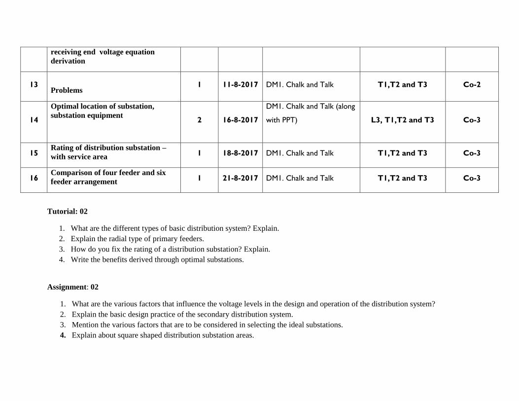
receiving end voltage equation
derivation
13
Problems 1 11-8-2017 DM1. Chalk and Talk T1,T2 and T3 Co-2
14
Optimal location of substation,
substation equipment
2 16-8-2017
DM1. Chalk and Talk (along
with PPT)
L3, T1,T2 and T3 Co-3
15 Rating of distribution substation –
with service area 1 18-8-2017 DM1. Chalk and Talk T1,T2 and T3 Co-3
16 Comparison of four feeder and six
feeder arrangement 1 21-8-2017 DM1. Chalk and Talk T1,T2 and T3 Co-3
Tutorial: 02
1. What are the different types of basic distribution system? Explain.
2. Explain the radial type of primary feeders.
3. How do you fix the rating of a distribution substation? Explain.
4. Write the benefits derived through optimal substations.
Assignment: 02
1. What are the various factors that influence the voltage levels in the design and operation of the distribution system?
2. Explain the basic design practice of the secondary distribution system.
3. Mention the various factors that are to be considered in selecting the ideal substations.
4. Explain about square shaped distribution substation areas.
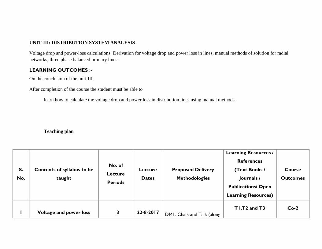
UNIT-III: DISTRIBUTION SYSTEM ANALYSIS
Voltage drop and power-loss calculations: Derivation for voltage drop and power loss in lines, manual methods of solution for radial
networks, three phase balanced primary lines.
LEARNING OUTCOMES :-
On the conclusion of the unit-III,
After completion of the course the student must be able to
learn how to calculate the voltage drop and power loss in distribution lines using manual methods.
Teaching plan
S.
No.
Contents of syllabus to be
taught
No. of
Lecture
Periods
Lecture
Dates
Proposed Delivery
Methodologies
Learning Resources /
References
(Text Books /
Journals /
Publications/ Open
Learning Resources)
Course
Outcomes
1
Voltage and power loss
3
22-8-2017
DM1. Chalk and Talk (along
T1,T2 and T3 Co-2
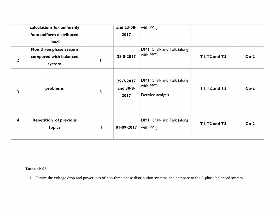
calculations for uniformly
/non uniform distributed
load
and 23-08-
2017
with PPT)
2
Non three phase system
compared with balanced
system
1
28-8-2017
DM1. Chalk and Talk (along
with PPT) T1,T2 and T3 Co-2
3 problems
3
29-7-2017
and 30-8-
2017
DM1. Chalk and Talk (along
with PPT)
Detailed analysis
T1,T2 and T3 Co-2
4
Repetition of previous
topics
1
01-09-2017
DM1. Chalk and Talk (along
with PPT)
T1,T2 and T3 Co-2
Tutorial: 03
1. Derive the voltage drop and power loss of non-three phase distribution systems and compare to the 3-phase balanced system.
2. Illustrate the computation of the voltage drop of a balanced three-phase feeder, supplied at one end in terms of the load and the
line parameters.
Assignment: 03
1. Derive the expression for voltage drop and power loss for non-uniformly radial type distribution load.
2. Derive the expression for the total series voltage drop and total copper loss per phase of a uniformly distributed load. Give the
assumptions made, if any.
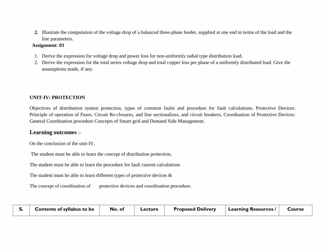
UNIT-IV: PROTECTION
Objectives of distribution system protection, types of common faults and procedure for fault calculations. Protective Devices:
Principle of operation of Fuses, Circuit Re-closures, and line sectionalizes, and circuit breakers, Coordination of Protective Devices:
General Coordination procedure Concepts of Smart grid and Demand Side Management.
Learning outcomes :-
On the conclusion of the unit-IV,
The student must be able to learn the concept of distribution protection,
The student must be able to learn the procedure for fault current calculations
The student must be able to learn different types of protective devices &
The concept of coordination of protective devices and coordination procedure.
S. Contents of syllabus to be No. of Lecture Proposed Delivery Learning Resources / Course
No. taught Lecture
Periods
Dates Methodologies References
(Text Books /
Journals /
Publications/ Open
Learning Resources)
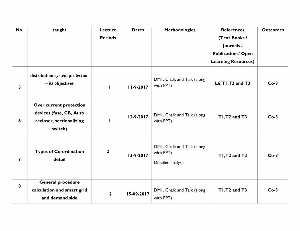
Outcomes
5
distribution system protection
– its objectives
1
11-9-2017
DM1. Chalk and Talk (along
with PPT)
L6,T1,T2 and T3 Co-3
6
Over current protection
devices (fuse, CB, Auto
recloser, sectionalizing
switch)
1
12-9-2017
DM1. Chalk and Talk (along
with PPT) T1,T2 and T3 Co-3
7
Types of Co-ordination
detail
2
13-9-2017
DM1. Chalk and Talk (along
with PPT)
Detailed analysis
T1,T2 and T3 Co-3
8
General procedure
calculation and smart grid
and demand side
2
15-09-2017
DM1. Chalk and Talk (along
with PPT)
T1,T2 and T3 Co-3
management
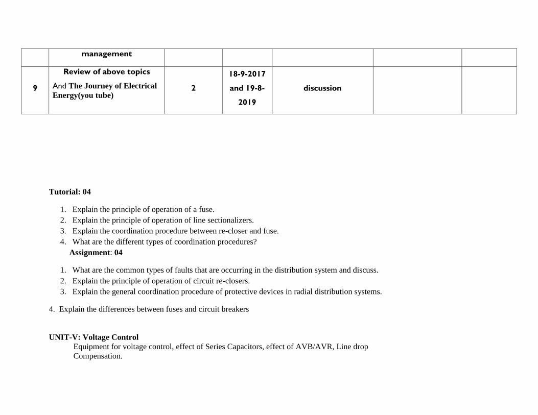
9
Review of above topics
And The Journey of Electrical
Energy(you tube)
2
18-9-2017
and 19-8-
2019
discussion
Tutorial: 04
1. Explain the principle of operation of a fuse.
2. Explain the principle of operation of line sectionalizers.
3. Explain the coordination procedure between re-closer and fuse.
4. What are the different types of coordination procedures?
Assignment: 04
1. What are the common types of faults that are occurring in the distribution system and discuss.
2. Explain the principle of operation of circuit re-closers.
3. Explain the general coordination procedure of protective devices in radial distribution systems.
4. Explain the differences between fuses and circuit breakers
UNIT-V: Voltage Control
Equipment for voltage control, effect of Series Capacitors, effect of AVB/AVR, Line drop
Compensation.

Distribution Automation: Need for DA, Objectives & Functions of DA,SCADA, Consumer information service, GIS,
Automatic meter reading.
Learning outcomes:-
On the conclusion of the unit-V,
• The student must be able to learn the concept of capacitive compensation for power factor correction and procedure
for best capacitor location.
• The student must be able to learn the concept of voltage control and the different types of control methods adopted for the
voltage control.
S.
No.
Contents of syllabus to be
taught
No. of
Lecture
Periods
Lecture
Dates
Proposed Delivery
Methodologies
Learning Resources /
References
(Text Books /
Journals /
Publications/ Open
Learning Resources)
Course
Outcomes
1
Importance of voltage
control and methods
1
22-9-2017
DM1. Chalk and Talk (along
with PPT)
L4, T1,T2 and T3 Co-4
2
Capacitor connected at the
load discuss phasor
diagrams
1
25-9-2017
DM1. Chalk and Talk (along
with PPT)
L4,T1,T2 and T3 Co-4
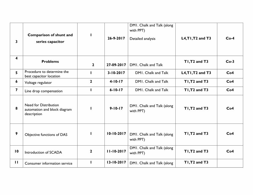
3
Comparison of shunt and
series capacitor
1
26-9-2017
DM1. Chalk and Talk (along
with PPT)
Detailed analysis
L4,T1,T2 and T3 Co-4
4
Problems
2
27-09-2017
DM1. Chalk and Talk T1,T2 and T3 Co-3
5 Procedure to determine the
best capacitor location 1 3-10-2017 DM1. Chalk and Talk L4,T1,T2 and T3 Co4
6 Voltage regulator 2 4-10-17 DM1. Chalk and Talk T1,T2 and T3 Co4
7 Line drop compensation 1 6-10-17 DM1. Chalk and Talk T1,T2 and T3 Co4
8 Need for Distribution
automation and block diagram
description
1 9-10-17
DM1. Chalk and Talk (along
with PPT)
T1,T2 and T3 Co4
9 Objective functions of DAS 1 10-10-2017
DM1. Chalk and Talk (along
with PPT)
T1,T2 and T3 Co4
10 Introduction of SCADA 2 11-10-2017 DM1. Chalk and Talk (along
with PPT) T1,T2 and T3 Co4
11 Consumer information service 1 13-10-2017 DM1. Chalk and Talk (along T1,T2 and T3
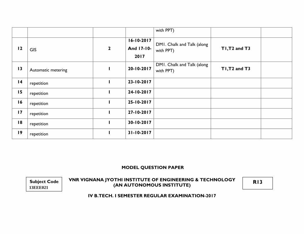
with PPT)
12 GIS 2
16-10-2017
And 17-10-
2017
DM1. Chalk and Talk (along
with PPT) T1,T2 and T3
13 Automatic metering 1 20-10-2017 DM1. Chalk and Talk (along
with PPT) T1,T2 and T3
14 repetition 1 23-10-2017
15 repetition 1 24-10-2017
16 repetition 1 25-10-2017
17 repetition 1 27-10-2017
18 repetition 1 30-10-2017
19 repetition 1 31-10-2017
MODEL QUESTION PAPER
VNR VIGNANA JYOTHI INSTITUTE OF ENGINEERING & TECHNOLOGY
(AN AUTONOMOUS INSTITUTE)
IV B.TECH. I SEMESTER REGULAR EXAMINATION-2017
Subject Code
13EEE021 R13
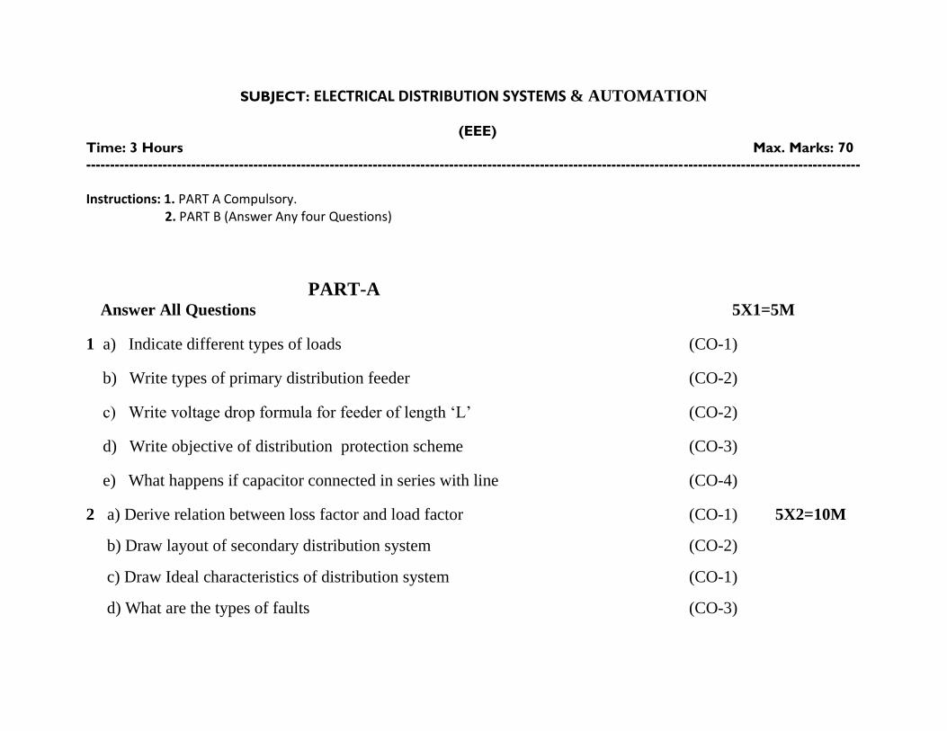
SUBJECT: ELECTRICAL DISTRIBUTION SYSTEMS & AUTOMATION
(EEE)
Time: 3 Hours Max. Marks: 70
------------------------------------------------------------------------------------------------------------------------------------------------------------------
Instructions: 1. PART A Compulsory.
2. PART B (Answer Any four Questions)
PART-A Answer All Questions 5X1=5M
1 a) Indicate different types of loads (CO-1)
b) Write types of primary distribution feeder (CO-2)
c) Write voltage drop formula for feeder of length ‘L’ (CO-2)
d) Write objective of distribution protection scheme (CO-3)
e) What happens if capacitor connected in series with line (CO-4)
2 a) Derive relation between loss factor and load factor (CO-1) 5X2=10M
b) Draw layout of secondary distribution system (CO-2)
c) Draw Ideal characteristics of distribution system (CO-1)
d) What are the types of faults (CO-3)
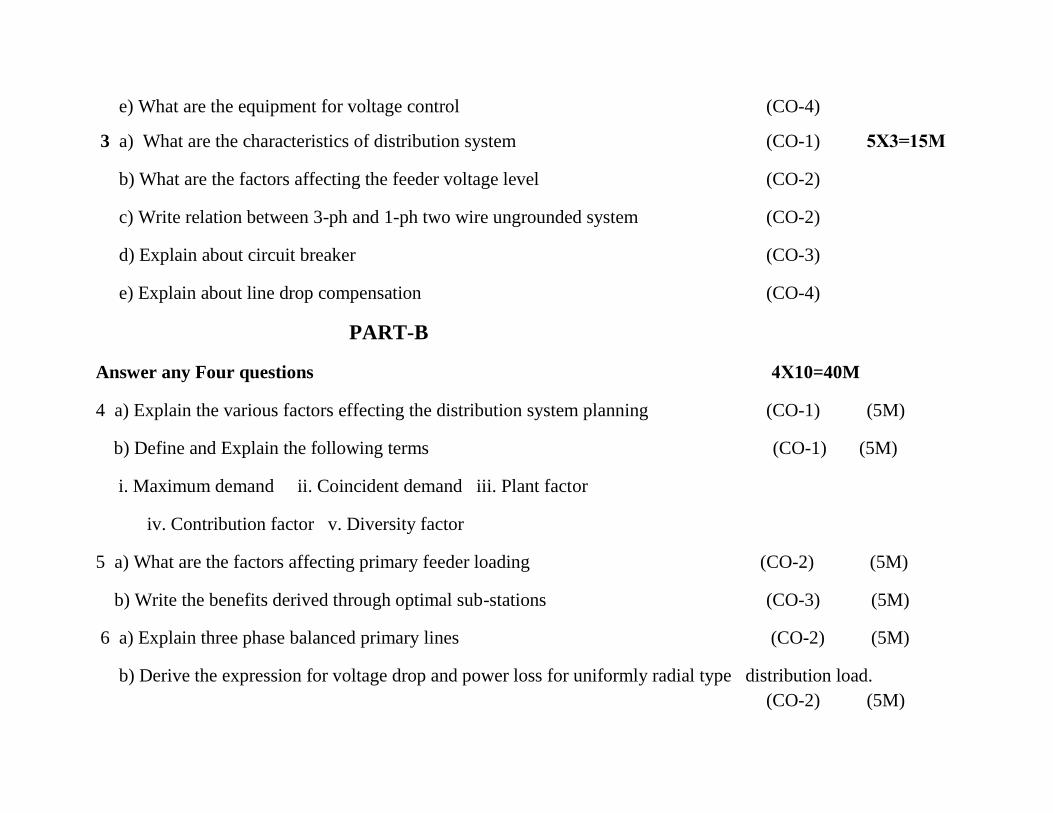
e) What are the equipment for voltage control (CO-4)
3 a) What are the characteristics of distribution system (CO-1) 5Х3=15M
b) What are the factors affecting the feeder voltage level (CO-2)
c) Write relation between 3-ph and 1-ph two wire ungrounded system (CO-2)
d) Explain about circuit breaker (CO-3)
e) Explain about line drop compensation (CO-4)
PART-B
Answer any Four questions 4Х10=40M
4 a) Explain the various factors effecting the distribution system planning (CO-1) (5M)
b) Define and Explain the following terms (CO-1) (5M)
i. Maximum demand ii. Coincident demand iii. Plant factor
iv. Contribution factor v. Diversity factor
5 a) What are the factors affecting primary feeder loading (CO-2) (5M)
b) Write the benefits derived through optimal sub-stations (CO-3) (5M)
6 a) Explain three phase balanced primary lines (CO-2) (5M)
b) Derive the expression for voltage drop and power loss for uniformly radial type distribution load.
(CO-2) (5M)
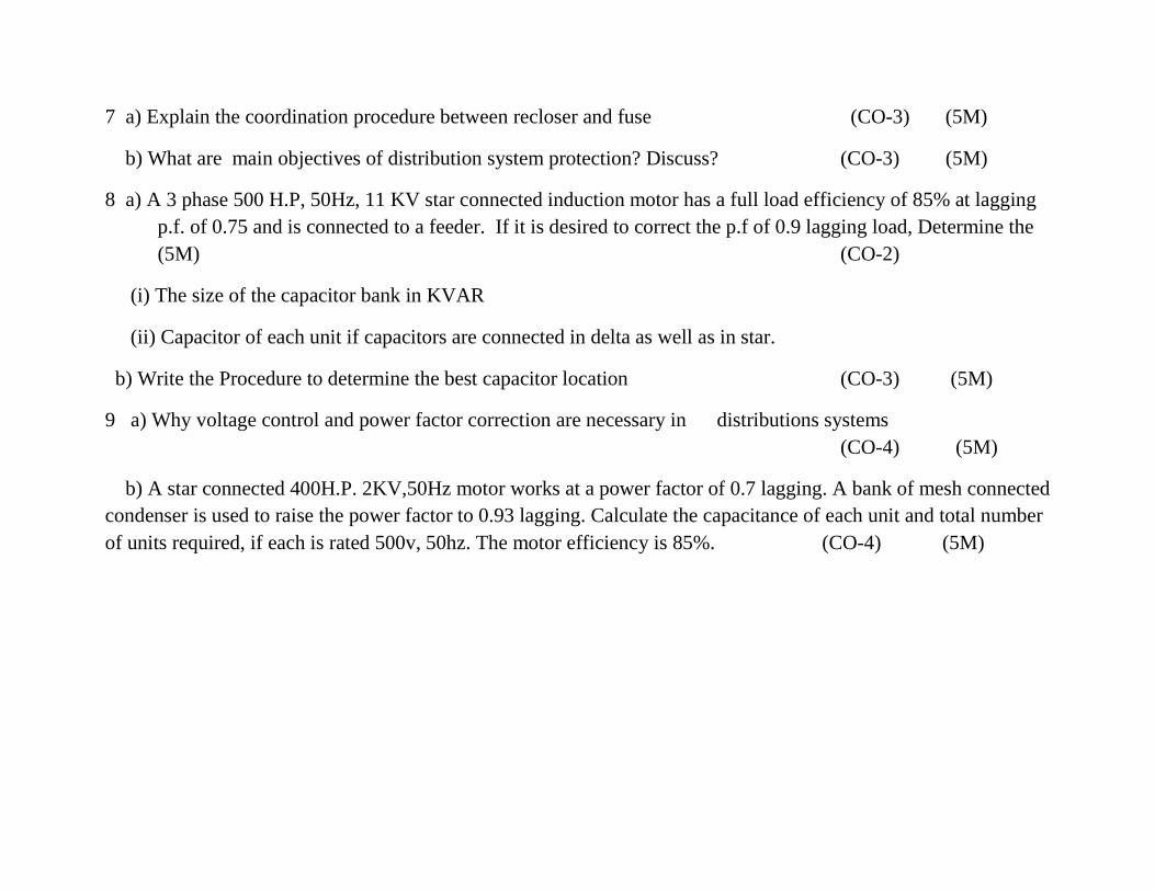
7 a) Explain the coordination procedure between recloser and fuse (CO-3) (5M)
b) What are main objectives of distribution system protection? Discuss? (CO-3) (5M)
8 a) A 3 phase 500 H.P, 50Hz, 11 KV star connected induction motor has a full load efficiency of 85% at lagging
p.f. of 0.75 and is connected to a feeder. If it is desired to correct the p.f of 0.9 lagging load, Determine the
(5M) (CO-2)
(i) The size of the capacitor bank in KVAR
(ii) Capacitor of each unit if capacitors are connected in delta as well as in star.
b) Write the Procedure to determine the best capacitor location (CO-3) (5M)
9 a) Why voltage control and power factor correction are necessary in distributions systems
(CO-4) (5M)
b) A star connected 400H.P. 2KV,50Hz motor works at a power factor of 0.7 lagging. A bank of mesh connected
condenser is used to raise the power factor to 0.93 lagging. Calculate the capacitance of each unit and total number
of units required, if each is rated 500v, 50hz. The motor efficiency is 85%. (CO-4) (5M)
VNR VIGNANA JYOTHI INSTITUTE OF ENGINEERING AND TECHNOLOGY
BACHUPALLY, NIZAMPET (S.O), HYDERABAD – 500090
LESSON PLAN: 2017-18
IV B. Tech : I Sem : EEE-1 L T/P/D C
3 1 4
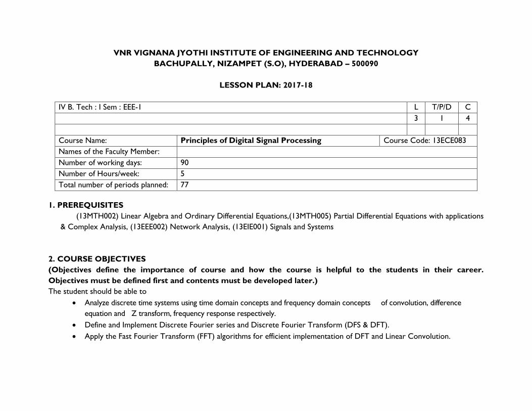
Course Name: Principles of Digital Signal Processing Co Course Code: 13ECE083
Names of the Faculty Member:
Number of working days: 90
Number of Hours/week: 5
Total number of periods planned: 77
1. PREREQUISITES
(13MTH002) Linear Algebra and Ordinary Differential Equations,(13MTH005) Partial Differential Equations with applications
& Complex Analysis, (13EEE002) Network Analysis, (13EIE001) Signals and Systems
2. COURSE OBJECTIVES
(Objectives define the importance of course and how the course is helpful to the students in their career.
Objectives must be defined first and contents must be developed later.)
The student should be able to
• Analyze discrete time systems using time domain concepts and frequency domain concepts of convolution, difference
equation and Z transform, frequency response respectively.
• Define and Implement Discrete Fourier series and Discrete Fourier Transform (DFS & DFT).
• Apply the Fast Fourier Transform (FFT) algorithms for efficient implementation of DFT and Linear Convolution.
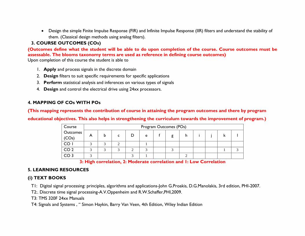
• Design the simple Finite Impulse Response (FIR) and Infinite Impulse Response (IIR) filters and understand the stability of
them. (Classical design methods using analog filters).
3. COURSE OUTCOMES (COs)
(Outcomes define what the student will be able to do upon completion of the course. Course outcomes must be
assessable. The blooms taxonomy terms are used as reference in defining course outcomes)
Upon completion of this course the student is able to
1. Apply and process signals in the discrete domain
2. Design filters to suit specific requirements for specific applications
3. Perform statistical analysis and inferences on various types of signals
4. Design and control the electrical drive using 24xx processors.
4. MAPPING OF COs WITH POs
(This mapping represents the contribution of course in attaining the program outcomes and there by program
educational objectives. This also helps in strengthening the curriculum towards the improvement of program.)
Course
Outcomes
(COs)
Program Outcomes (POs)
A b c D e f g h i j k l
CO 1 3 3 2
1
CO 2 3 3 3 2 3
3
1 3
CO 3 3
3 1
2
3: High correlation, 2: Moderate correlation and 1: Low Correlation
5. LEARNING RESOURCES
(i) TEXT BOOKS
T1: Digital signal processing: principles, algorithms and applications-John G.Proakis, D.G.Manolakis, 3rd edition, PHI-2007.
T2:. Discrete time signal processing-A.V.Oppenheim and R.W.Schaffer,PHI,2009.
T3: TMS 320F 24xx Manuals
T4: Signals and Systems , “ Simon Haykin, Barry Van Veen, 4th Edition, Wiley Indian Edition

T5: Ramesh Babu, “Digital Signal Processing”, SCITECH Publications, 4th Edition, 2009.
T6: Digital signal processing-S.Salivahanan, A.Vallavaraj, C.Gnanapriya, TMH, 2009.
(ii) REFERENCES (Publications/ Open Learning Resources)
(Course delivery including latest trends brings good insight of the course in students and also inculcates the habit of
self learning among the students.
Publications referred can be given unit wise or at course level.)
R1: Fundamentals of digital signal processing using MATLAB-Robert J.Schilling, Sandra L.Harris, Thomson, 2007.
R2: Discrete systems and digital signal processing with MATLAB-Taan S.ElAli,CRC Press,2009.
R3: P Venkata Ramani, M.Bhaskar, “Digital Signal Processor; Architecture, Programming & Application”, TataMcGrawHill-2001
R4: Digital Signal Processor using MATLAB, Vinay. K. Ingle, John.G.Proakis, International Student Editon
R5: Schaum’s Outlines “ Digital Signal Processing, Monson.H.Hayes, Tata Mc Graw Hill Edition, 2004
(a) Publications
P1. Digital signal processing-Fundamentals and applications-LiTan, Elsevier,2008.
(b) Open Learning Resources for self learning
L1. https://www.youtube.com/watch?v=6dFnpz_AEyA&list=PLF0B227275B5E6D3D
L2. https://www.youtube.com/watch?v=rkvEM5Y3N60&list=PL738F5EDE345AD26F
L3. https://www.youtube.com/watch?v=4ufeTZ6fSNY&list=PLbMVogVj5nJRY7X-tMNDHPGdmfZyfHC7J
(iii) JOURNALS
J1.

6. DELIVERY METHODOLOGIES
(Depending on the suitability to the delivery of concept, one or more among the following delivery methodologies
are adopted to engage the student in learning)
DM1: Chalk and Talk DM5: Open The Box
DM2: Learning by doing DM6: Case Study
DM3: Collaborative Learning (Think Pair Share, POGIL, etc.) DM7: Group Project
DM4: Demonstration (Physical / Laboratory / Audio Visuals) DM8: Any other
7. PROPOSED FIELD VISITS/ GUEST LECTURE BY INDUSTRY EXPERT
(To be added for the courses as directed by the department.)
Guest Lecture: "Applications of Digital Signal Processing in Image, radar and bio medical signal processing by Dr.P.Srihari,
Professor/ECE Depatment, VNRVJIET on 19-08-2017
8. ASSESSMENT
(As per Regulations, AM1 and AM2 are compulsory for assessment. Whereas, any two or more assessment
methodologies can be considered from AM3 to AM9 under assignment towards continuous assessment of the
performance of students.)
AM1: Semester End Examination . AM2: Mid Term Examination
AM3: Home Assignments AM4: Open Book Test
AM6: Objective Test AM6: Quizzes
AM7: Course Projects** AM8: Group Presentations
AM9: Any other (Specify)
** (To be added for the courses as directed by the department. The no. of course projects is left to the liberty of
faculty)
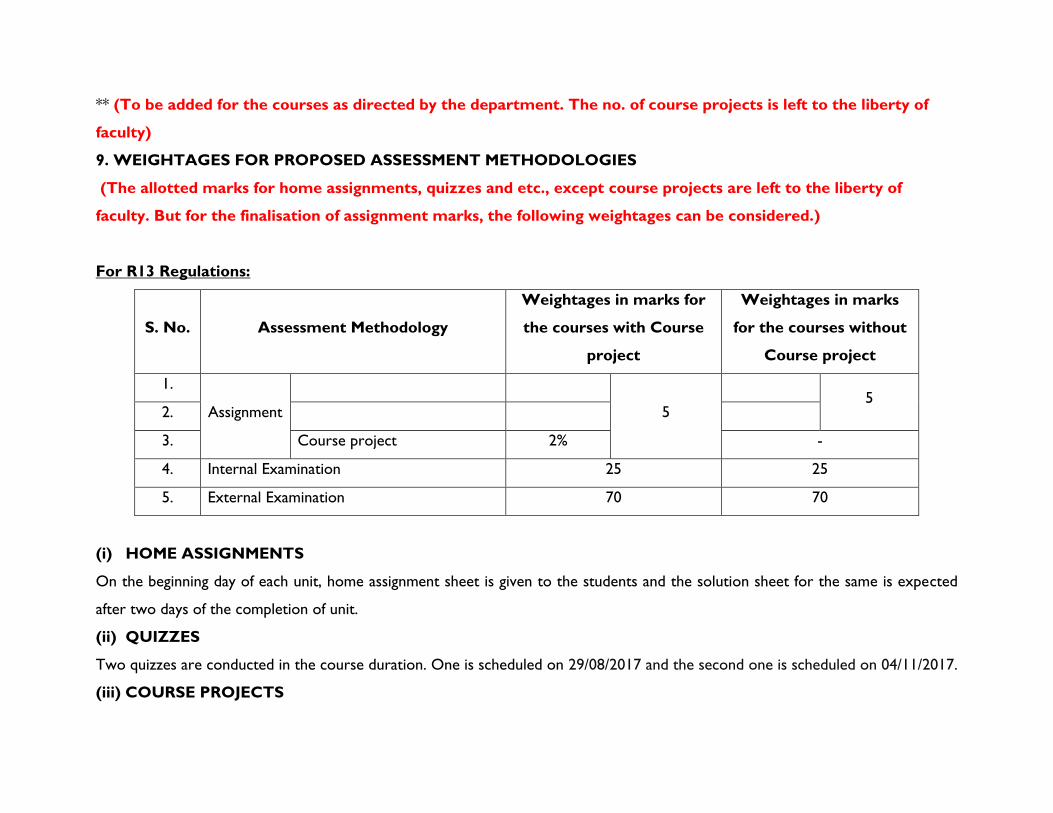
9. WEIGHTAGES FOR PROPOSED ASSESSMENT METHODOLOGIES
(The allotted marks for home assignments, quizzes and etc., except course projects are left to the liberty of
faculty. But for the finalisation of assignment marks, the following weightages can be considered.)
For R13 Regulations:
S. No. Assessment Methodology
Weightages in marks for
the courses with Course
project
Weightages in marks
for the courses without
Course project
1.
Assignment
5
5
2.
3. Course project 2% -
4. Internal Examination 25 25
5. External Examination 70 70
(i) HOME ASSIGNMENTS
On the beginning day of each unit, home assignment sheet is given to the students and the solution sheet for the same is expected
after two days of the completion of unit.
(ii) QUIZZES
Two quizzes are conducted in the course duration. One is scheduled on 29/08/2017 and the second one is scheduled on 04/11/2017.
(iii) COURSE PROJECTS
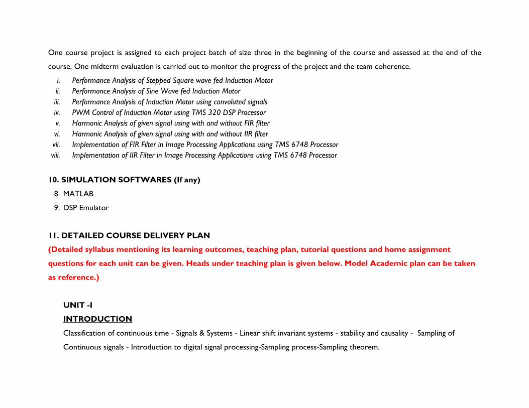
One course project is assigned to each project batch of size three in the beginning of the course and assessed at the end of the
course. One midterm evaluation is carried out to monitor the progress of the project and the team coherence.
i. Performance Analysis of Stepped Square wave fed Induction Motor
ii. Performance Analysis of Sine Wave fed Induction Motor
iii. Performance Analysis of Induction Motor using convoluted signals
iv. PWM Control of Induction Motor using TMS 320 DSP Processor
v. Harmonic Analysis of given signal using with and without FIR filter
vi. Harmonic Analysis of given signal using with and without IIR filter
vii. Implementation of FIR Filter in Image Processing Applications using TMS 6748 Processor
viii. Implementation of IIR Filter in Image Processing Applications using TMS 6748 Processor
10. SIMULATION SOFTWARES (If any)
8. MATLAB
9. DSP Emulator
11. DETAILED COURSE DELIVERY PLAN
(Detailed syllabus mentioning its learning outcomes, teaching plan, tutorial questions and home assignment
questions for each unit can be given. Heads under teaching plan is given below. Model Academic plan can be taken
as reference.)
UNIT -I
INTRODUCTION
Classification of continuous time - Signals & Systems - Linear shift invariant systems - stability and causality - Sampling of
Continuous signals - Introduction to digital signal processing-Sampling process-Sampling theorem.
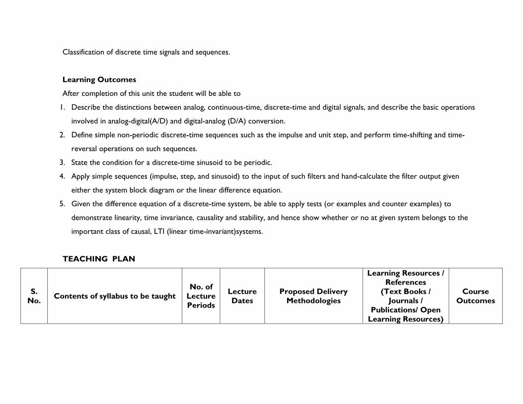
Classification of discrete time signals and sequences.
Learning Outcomes
After completion of this unit the student will be able to
1. Describe the distinctions between analog, continuous-time, discrete-time and digital signals, and describe the basic operations
involved in analog-digital(A/D) and digital-analog (D/A) conversion.
2. Define simple non-periodic discrete-time sequences such as the impulse and unit step, and perform time-shifting and time-
reversal operations on such sequences.
3. State the condition for a discrete-time sinusoid to be periodic.
4. Apply simple sequences (impulse, step, and sinusoid) to the input of such filters and hand-calculate the filter output given
either the system block diagram or the linear difference equation.
5. Given the difference equation of a discrete-time system, be able to apply tests (or examples and counter examples) to
demonstrate linearity, time invariance, causality and stability, and hence show whether or no at given system belongs to the
important class of causal, LTI (linear time-invariant)systems.
TEACHING PLAN
S.
No. Contents of syllabus to be taught
No. of
Lecture
Periods
Lecture
Dates
Proposed Delivery
Methodologies
Learning Resources /
References
(Text Books /
Journals /
Publications/ Open
Learning Resources)
Course
Outcomes
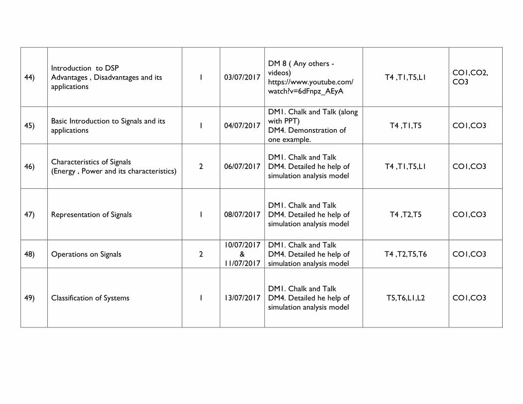
44) Introduction to DSP
Advantages , Disadvantages and its
applications
1 03/07/2017
DM 8 ( Any others -
videos)
https://www.youtube.com/
watch?v=6dFnpz_AEyA
T4 ,T1,T5,L1 CO1,CO2,
CO3
45) Basic Introduction to Signals and its
applications 1 04/07/2017
DM1. Chalk and Talk (along
with PPT)
DM4. Demonstration of
one example.
T4 ,T1,T5 CO1,CO3
46) Characteristics of Signals
(Energy , Power and its characteristics) 2 06/07/2017
DM1. Chalk and Talk
DM4. Detailed he help of
simulation analysis model
T4 ,T1,T5,L1 CO1,CO3
47) Representation of Signals 1 08/07/2017
DM1. Chalk and Talk
DM4. Detailed he help of
simulation analysis model
T4 ,T2,T5 CO1,CO3
48) Operations on Signals 2
10/07/2017
&
11/07/2017
DM1. Chalk and Talk
DM4. Detailed he help of
simulation analysis model
T4 ,T2,T5,T6 CO1,CO3
49) Classification of Systems 1 13/07/2017
DM1. Chalk and Talk
DM4. Detailed he help of
simulation analysis model
T5,T6,L1,L2 CO1,CO3
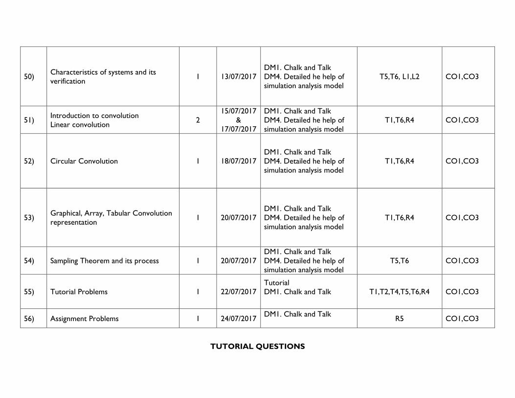
50) Characteristics of systems and its
verification 1 13/07/2017
DM1. Chalk and Talk
DM4. Detailed he help of
simulation analysis model
T5,T6, L1,L2 CO1,CO3
51) Introduction to convolution
Linear convolution 2
15/07/2017
&
17/07/2017
DM1. Chalk and Talk
DM4. Detailed he help of
simulation analysis model
T1,T6,R4 CO1,CO3
52) Circular Convolution 1 18/07/2017
DM1. Chalk and Talk
DM4. Detailed he help of
simulation analysis model
T1,T6,R4 CO1,CO3
53) Graphical, Array, Tabular Convolution
representation 1 20/07/2017
DM1. Chalk and Talk
DM4. Detailed he help of
simulation analysis model
T1,T6,R4 CO1,CO3
54) Sampling Theorem and its process 1 20/07/2017
DM1. Chalk and Talk
DM4. Detailed he help of
simulation analysis model
T5,T6 CO1,CO3
55) Tutorial Problems 1 22/07/2017
Tutorial
DM1. Chalk and Talk
T1,T2,T4,T5,T6,R4 CO1,CO3
56) Assignment Problems 1 24/07/2017 DM1. Chalk and Talk
R5 CO1,CO3
TUTORIAL QUESTIONS
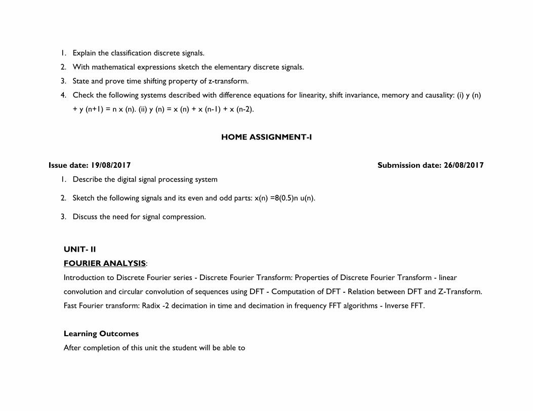
1. Explain the classification discrete signals.
2. With mathematical expressions sketch the elementary discrete signals.
3. State and prove time shifting property of z-transform.
4. Check the following systems described with difference equations for linearity, shift invariance, memory and causality: (i) y (n)
+ y (n+1) = n x (n). (ii) y (n) = x (n) + x (n-1) + x (n-2).
HOME ASSIGNMENT-I
Issue date: 19/08/2017 Submission date: 26/08/2017
1. Describe the digital signal processing system
2. Sketch the following signals and its even and odd parts: x(n) =8(0.5)n u(n).
3. Discuss the need for signal compression.
UNIT- II
FOURIER ANALYSIS:
Introduction to Discrete Fourier series - Discrete Fourier Transform: Properties of Discrete Fourier Transform - linear
convolution and circular convolution of sequences using DFT - Computation of DFT - Relation between DFT and Z-Transform.
Fast Fourier transform: Radix -2 decimation in time and decimation in frequency FFT algorithms - Inverse FFT.
Learning Outcomes
After completion of this unit the student will be able to
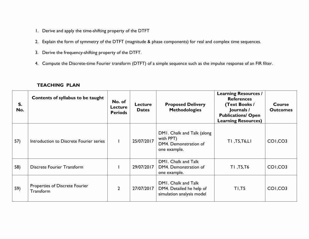
1. Derive and apply the time-shifting property of the DTFT
2. Explain the form of symmetry of the DTFT (magnitude & phase components) for real and complex time sequences.
3. Derive the frequency-shifting property of the DTFT.
4. Compute the Discrete-time Fourier transform (DTFT) of a simple sequence such as the impulse response of an FIR filter.
TEACHING PLAN
S.
No.
Contents of syllabus to be taught
No. of
Lecture
Periods
Lecture
Dates
Proposed Delivery
Methodologies
Learning Resources /
References
(Text Books /
Journals /
Publications/ Open
Learning Resources)
Course
Outcomes
57) Introduction to Discrete Fourier series 1 25/07/2017
DM1. Chalk and Talk (along
with PPT)
DM4. Demonstration of
one example.
T1 ,T5,T6,L1 CO1,CO3
58) Discrete Fourier Transform 1 29/07/2017
DM1. Chalk and Talk
DM4. Demonstration of
one example.
T1 ,T5,T6 CO1,CO3
59) Properties of Discrete Fourier
Transform 2 27/07/2017
DM1. Chalk and Talk
DM4. Detailed he help of
simulation analysis model
T1,T5 CO1,CO3

60) linear convolution with problems 2
31/07/2017
&
01/08/2017
DM1. Chalk and Talk
DM4. Detailed he help of
simulation analysis model
T1,T5,R4 CO1,CO3
61) circular convolution with problems 2 03/08/2017
DM1. Chalk and Talk
DM4. Detailed he help of
simulation analysis model
T1 ,T5,T6,R4 CO1,CO3
62) Computation of DFT 1 07/08/2017
DM1. Chalk and Talk
DM4. Detailed he help of
simulation analysis model
T1,T5 CO1,CO3
63) Relation between DFT and Z-Transform
1 08/08/2017 DM1. Chalk and Talk
T1,T5 CO1,CO3
64) DFT based problems 2 10/08/2017
DM1. Chalk and Talk
DM4. Detailed he help of
simulation analysis model
T1,T5,T6 CO1,CO3
65) Introduction to Fast Fourier Transform 1 11/08/2017 DM1. Chalk and Talk T1,T5 CO1,CO3
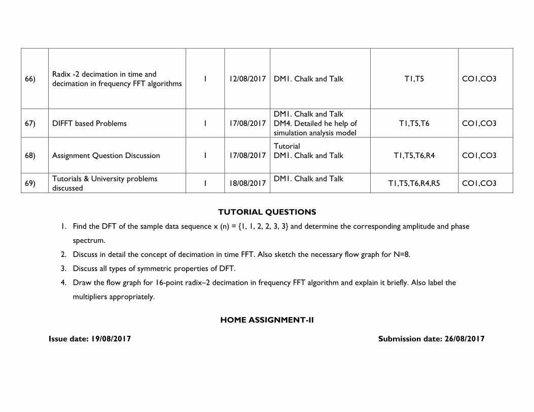
66) Radix -2 decimation in time and
decimation in frequency FFT algorithms 1 12/08/2017 DM1. Chalk and Talk T1,T5 CO1,CO3
67) DIFFT based Problems 1 17/08/2017
DM1. Chalk and Talk
DM4. Detailed he help of
simulation analysis model
T1,T5,T6 CO1,CO3
68) Assignment Question Discussion 1 17/08/2017
Tutorial
DM1. Chalk and Talk
T1,T5,T6,R4 CO1,CO3
69) Tutorials & University problems
discussed 1 18/08/2017
DM1. Chalk and Talk
T1,T5,T6,R4,R5 CO1,CO3
TUTORIAL QUESTIONS
1. Find the DFT of the sample data sequence x (n) = 1, 1, 2, 2, 3, 3 and determine the corresponding amplitude and phase
spectrum.
2. Discuss in detail the concept of decimation in time FFT. Also sketch the necessary flow graph for N=8.
3. Discuss all types of symmetric properties of DFT.
4. Draw the flow graph for 16-point radix–2 decimation in frequency FFT algorithm and explain it briefly. Also label the
multipliers appropriately.
HOME ASSIGNMENT-II
Issue date: 19/08/2017 Submission date: 26/08/2017

1. Given the two sequences of length ‘4’ as under x(n) = 1,2,3,1 h(n) = 4,3,2,2. Verify the answer using DFT method.
2. Compare DIT-FFT and DIF-FFT algorithms.
3. State and prove circular convolution property of DFT.
4. Find DFT of sequence using DIT – FFT, the sequence is x (n) = 1, 1, 1, 1, 1, 1, 1, 1.
5. Compute the 4-point DFT of the sequence x (n) = (1, 0, 1, 0) using DIF-FFT radix – 2 algorithm. Compare the answer with
conventional approach.
UNIT- III
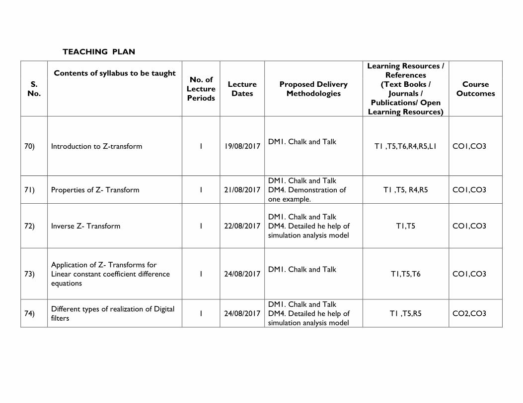
Z- TRANSFORM:
Introduction to Z-transform - Properties of Z- Transform - Inverse Z- Transform - Application of Z- Transforms for Linear
constant coefficient difference equations - Realization of Digital filters - system function – stability criterion.
Learning Outcomes
After completion of this unit the student will be able to
1. Calculate the z-transform X(z) of a simple sequence x(n) (such as exponentials and sinusoids): specify the region of
convergence (ROC) and the bounding poles of X(z).
2. Derive the time-shifting property of the z-transform
3. Given a z-transform X(z) and its ROC, state whether or not the DTFT of x(n) exists, and predict whether the sequence x(n)
is left-sided, right-sided, two-sided, and/or of finite duration.
4. Apply z-transform properties and theorems, notably convolution, time reversal, and multiplication by an exponential
sequence (plus time-shifting property listed earlier)
TEACHING PLAN
S.
No.
Contents of syllabus to be taught
No. of
Lecture
Periods
Lecture
Dates
Proposed Delivery
Methodologies
Learning Resources /
References
(Text Books /
Journals /
Publications/ Open
Learning Resources)
Course
Outcomes
70) Introduction to Z-transform 1 19/08/2017 DM1. Chalk and Talk
T1 ,T5,T6,R4,R5,L1 CO1,CO3
71) Properties of Z- Transform 1 21/08/2017
DM1. Chalk and Talk
DM4. Demonstration of
one example.
T1 ,T5, R4,R5 CO1,CO3
72) Inverse Z- Transform 1 22/08/2017
DM1. Chalk and Talk
DM4. Detailed he help of
simulation analysis model
T1,T5 CO1,CO3
73) Application of Z- Transforms for
Linear constant coefficient difference
equations
1 24/08/2017 DM1. Chalk and Talk
T1,T5,T6 CO1,CO3
74) Different types of realization of Digital
filters 1 24/08/2017
DM1. Chalk and Talk
DM4. Detailed he help of
simulation analysis model
T1 ,T5,R5 CO2,CO3
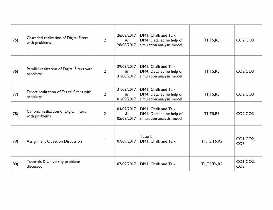
75) Cascaded realization of Digital filters
with problems 2
26/08/2017
&
28/08/2017
DM1. Chalk and Talk
DM4. Detailed he help of
simulation analysis model
T1,T5,R5 CO2,CO3
76) Parallel realization of Digital filters with
problems 2
29/08/2017
&
31/08/2017
DM1. Chalk and Talk
DM4. Detailed he help of
simulation analysis model
T1,T5,R5 CO2,CO3
77) Direct realization of Digital filters with
problems 2
31/08/2017
&
01/09/2017
DM1. Chalk and Talk
DM4. Detailed he help of
simulation analysis model
T1,T5,R5 CO2,CO3
78) Canonic realization of Digital filters
with problems 2
04/09/2017
&
05/09/2017
DM1. Chalk and Talk
DM4. Detailed he help of
simulation analysis model
T1,T5,R5 CO2,CO3
79) Assignment Question Discussion 1 07/09/2017
Tutorial
DM1. Chalk and Talk
T1,T5,T6,R5 CO1,CO2,
CO3
80) Tutorials & University problems
discussed 1 07/09/2017
DM1. Chalk and Talk
T1,T5,T6,R5 CO1,CO2,
CO3
TUTORIAL QUESTIONS
1. State and prove time shifting property of z-transform
2. Determine z-transform, ROC and pole-zero locations of x(n) = 𝛼𝛼n u(n) + βn u(-n-1).
3. Using backward difference method obtain H (z) for following H (s) = 1/(s + 3).
HOME ASSIGNMENT-III
Issue date: 23/09/2017 Submission date: 21/10/2017
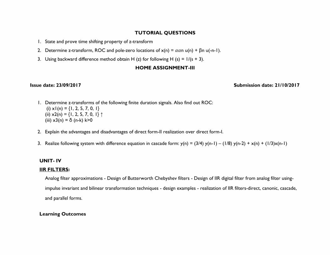
1. Determine z-transforms of the following finite duration signals. Also find out ROC:
(i) x1(n) = 1, 2, 5, 7, 0, 1
(ii) x2(n) = 1, 2, 5, 7, 0, 1 ↑
(iii) x3(n) = δ (n-k) k>0
2. Explain the advantages and disadvantages of direct form-II realization over direct form-I.
3. Realize following system with difference equation in cascade form: y(n) = (3/4) y(n-1) – (1/8) y(n-2) + x(n) + (1/3)x(n-1)
UNIT- IV
IIR FILTERS:
Analog filter approximations - Design of Butterworth Chebyshev filters - Design of IIR digital filter from analog filter using-
impulse invariant and bilinear transformation techniques - design examples - realization of IIR filters-direct, canonic, cascade,
and parallel forms.
Learning Outcomes
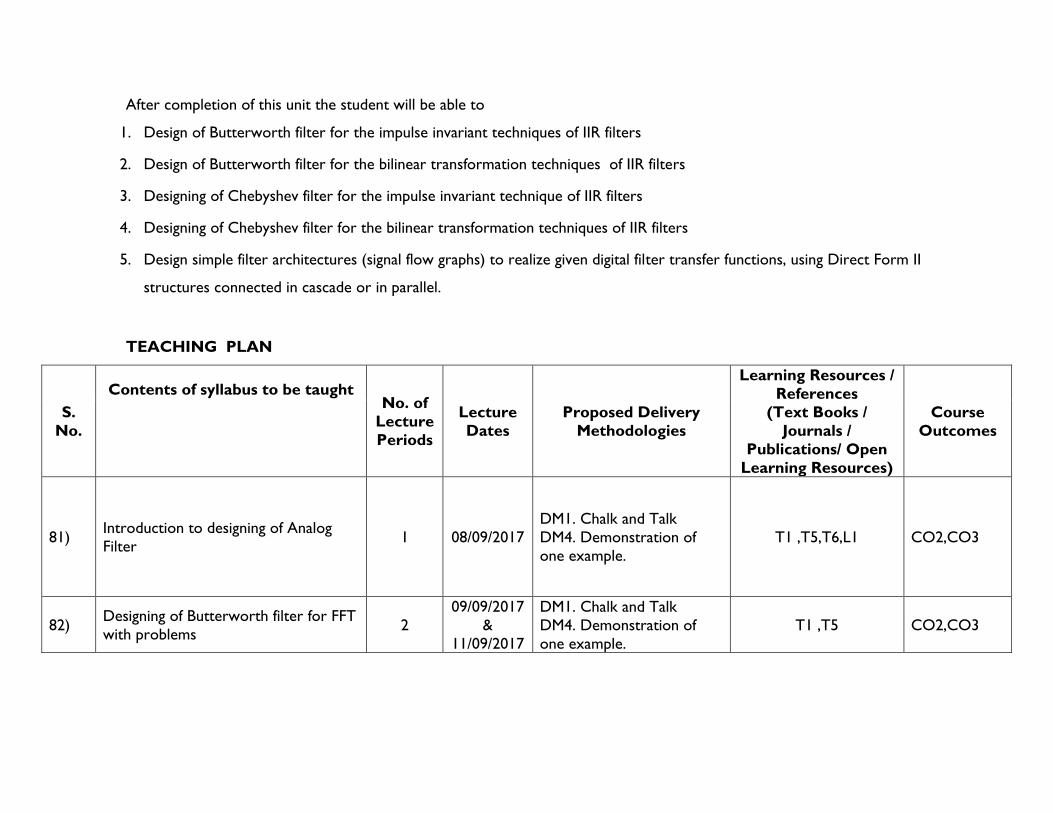
After completion of this unit the student will be able to
1. Design of Butterworth filter for the impulse invariant techniques of IIR filters
2. Design of Butterworth filter for the bilinear transformation techniques of IIR filters
3. Designing of Chebyshev filter for the impulse invariant technique of IIR filters
4. Designing of Chebyshev filter for the bilinear transformation techniques of IIR filters
5. Design simple filter architectures (signal flow graphs) to realize given digital filter transfer functions, using Direct Form II
structures connected in cascade or in parallel.
TEACHING PLAN
S.
No.
Contents of syllabus to be taught
No. of
Lecture
Periods
Lecture
Dates
Proposed Delivery
Methodologies
Learning Resources /
References
(Text Books /
Journals /
Publications/ Open
Learning Resources)
Course
Outcomes
81) Introduction to designing of Analog
Filter 1 08/09/2017
DM1. Chalk and Talk
DM4. Demonstration of
one example.
T1 ,T5,T6,L1 CO2,CO3
82) Designing of Butterworth filter for FFT
with problems 2
09/09/2017
&
11/09/2017
DM1. Chalk and Talk
DM4. Demonstration of
one example.
T1 ,T5 CO2,CO3
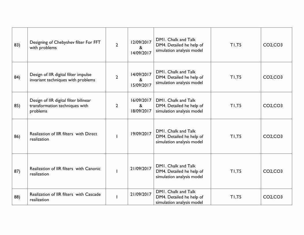
83) Designing of Chebyshev filter For FFT
with problems 2
12/09/2017
&
14/09/2017
DM1. Chalk and Talk
DM4. Detailed he help of
simulation analysis model
T1,T5 CO2,CO3
84) Design of IIR digital filter impulse
invariant techniques with problems 2
14/09/2017
&
15/09/2017
DM1. Chalk and Talk
DM4. Detailed he help of
simulation analysis model
T1,T5 CO2,CO3
85) Design of IIR digital filter bilinear
transformation techniques with
problems
2
16/09/2017
&
18/09/2017
DM1. Chalk and Talk
DM4. Detailed he help of
simulation analysis model
T1,T5 CO2,CO3
86) Realization of IIR filters with Direct
realization 1
19/09/2017
DM1. Chalk and Talk
DM4. Detailed he help of
simulation analysis model
T1,T5 CO2,CO3
87) Realization of IIR filters with Canonic
realization 1
21/09/2017
DM1. Chalk and Talk
DM4. Detailed he help of
simulation analysis model
T1,T5 CO2,CO3
88) Realization of IIR filters with Cascade
realization 1
21/09/2017
DM1. Chalk and Talk
DM4. Detailed he help of
simulation analysis model
T1,T5 CO2,CO3
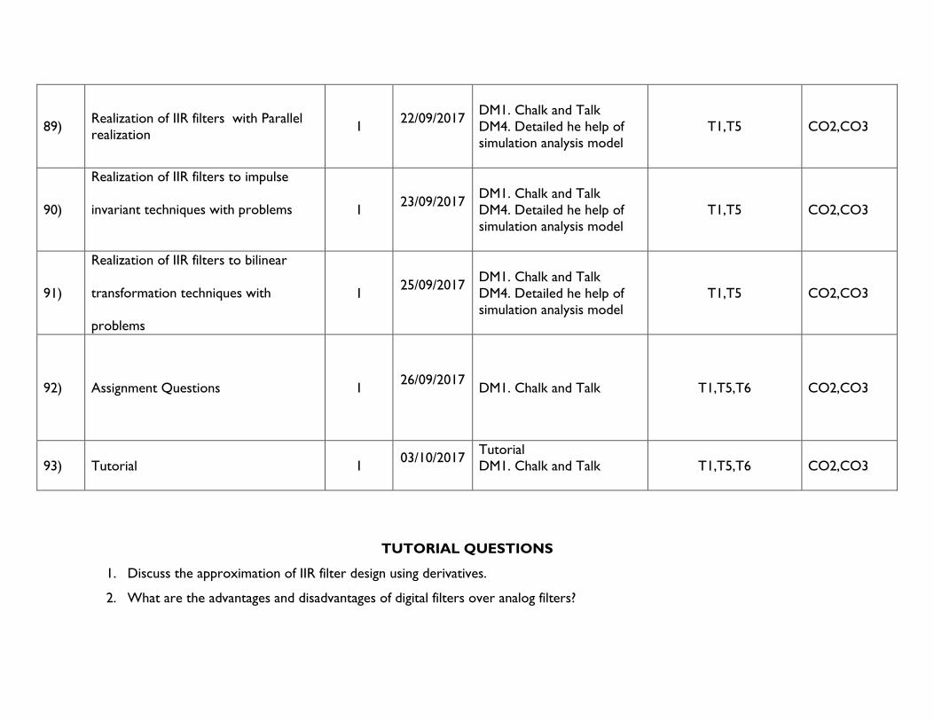
89) Realization of IIR filters with Parallel
realization 1
22/09/2017
DM1. Chalk and Talk
DM4. Detailed he help of
simulation analysis model
T1,T5 CO2,CO3
90)
Realization of IIR filters to impulse
invariant techniques with problems 1 23/09/2017
DM1. Chalk and Talk
DM4. Detailed he help of
simulation analysis model
T1,T5 CO2,CO3
91)
Realization of IIR filters to bilinear
transformation techniques with
problems
1 25/09/2017
DM1. Chalk and Talk
DM4. Detailed he help of
simulation analysis model
T1,T5 CO2,CO3
92) Assignment Questions 1 26/09/2017
DM1. Chalk and Talk
T1,T5,T6 CO2,CO3
93) Tutorial 1 03/10/2017
Tutorial
DM1. Chalk and Talk
T1,T5,T6 CO2,CO3
TUTORIAL QUESTIONS
1. Discuss the approximation of IIR filter design using derivatives.
2. What are the advantages and disadvantages of digital filters over analog filters?
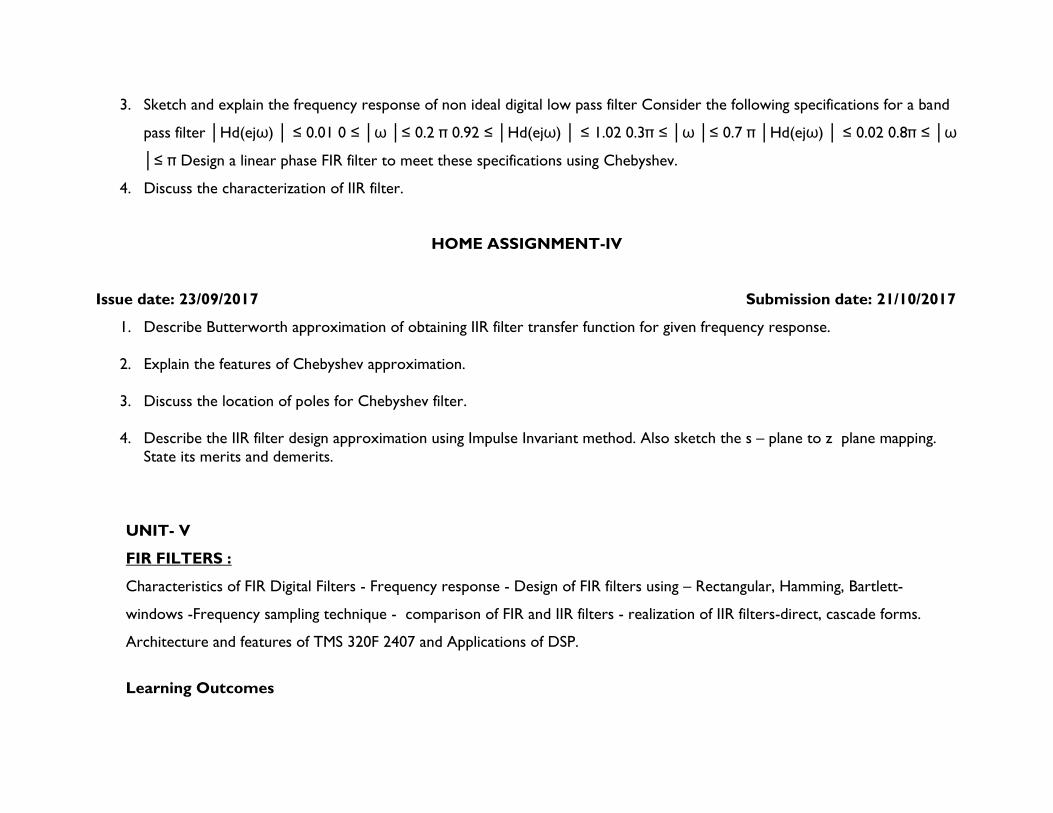
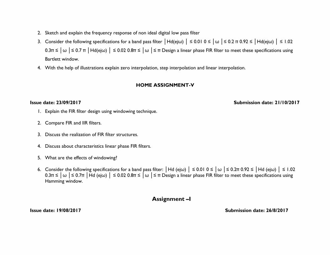
3. Sketch and explain the frequency response of non ideal digital low pass filter Consider the following specifications for a band
pass filter Hd(ejω) ≤ 0.01 0 ≤ ω ≤ 0.2 π 0.92 ≤ Hd(ejω) ≤ 1.02 0.3π ≤ ω ≤ 0.7 π Hd(ejω) ≤ 0.02 0.8π ≤ ω
≤ π Design a linear phase FIR filter to meet these specifications using Chebyshev.
4. Discuss the characterization of IIR filter.
HOME ASSIGNMENT-IV
Issue date: 23/09/2017 Submission date: 21/10/2017
1. Describe Butterworth approximation of obtaining IIR filter transfer function for given frequency response.
2. Explain the features of Chebyshev approximation.
3. Discuss the location of poles for Chebyshev filter.
4. Describe the IIR filter design approximation using Impulse Invariant method. Also sketch the s – plane to z plane mapping.
State its merits and demerits.
UNIT- V
FIR FILTERS :
Characteristics of FIR Digital Filters - Frequency response - Design of FIR filters using – Rectangular, Hamming, Bartlett-
windows -Frequency sampling technique - comparison of FIR and IIR filters - realization of IIR filters-direct, cascade forms.
Architecture and features of TMS 320F 2407 and Applications of DSP.
Learning Outcomes
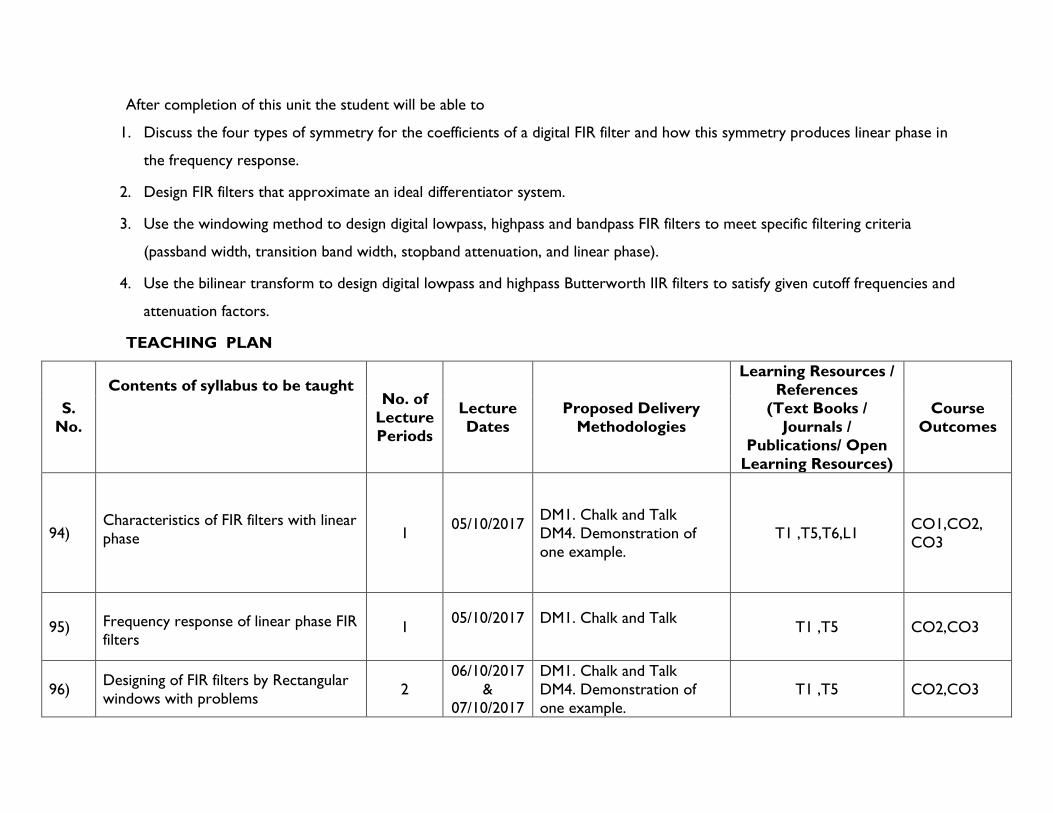
After completion of this unit the student will be able to
1. Discuss the four types of symmetry for the coefficients of a digital FIR filter and how this symmetry produces linear phase in
the frequency response.
2. Design FIR filters that approximate an ideal differentiator system.
3. Use the windowing method to design digital lowpass, highpass and bandpass FIR filters to meet specific filtering criteria
(passband width, transition band width, stopband attenuation, and linear phase).
4. Use the bilinear transform to design digital lowpass and highpass Butterworth IIR filters to satisfy given cutoff frequencies and
attenuation factors.
TEACHING PLAN
S.
No.
Contents of syllabus to be taught
No. of
Lecture
Periods
Lecture
Dates
Proposed Delivery
Methodologies
Learning Resources /
References
(Text Books /
Journals /
Publications/ Open
Learning Resources)
Course
Outcomes
94)
Characteristics of FIR filters with linear
phase 1 05/10/2017
DM1. Chalk and Talk
DM4. Demonstration of
one example.
T1 ,T5,T6,L1 CO1,CO2,
CO3
95)
Frequency response of linear phase FIR
filters 1
05/10/2017
DM1. Chalk and Talk
T1 ,T5 CO2,CO3
96) Designing of FIR filters by Rectangular
windows with problems 2
06/10/2017
&
07/10/2017
DM1. Chalk and Talk
DM4. Demonstration of
one example.
T1 ,T5 CO2,CO3
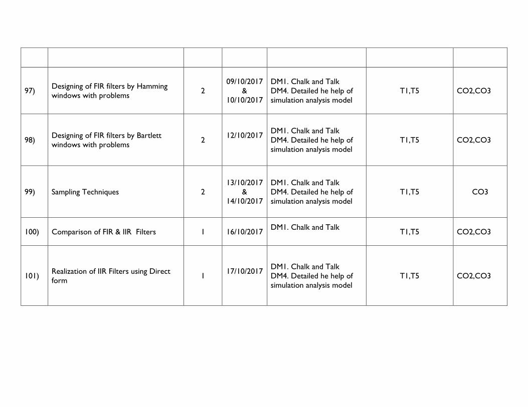
97) Designing of FIR filters by Hamming
windows with problems 2
09/10/2017
&
10/10/2017
DM1. Chalk and Talk
DM4. Detailed he help of
simulation analysis model
T1,T5 CO2,CO3
98) Designing of FIR filters by Bartlett
windows with problems 2
12/10/2017
DM1. Chalk and Talk
DM4. Detailed he help of
simulation analysis model
T1,T5 CO2,CO3
99) Sampling Techniques 2
13/10/2017
&
14/10/2017
DM1. Chalk and Talk
DM4. Detailed he help of
simulation analysis model
T1,T5 CO3
100) Comparison of FIR & IIR Filters 1
16/10/2017
DM1. Chalk and Talk
T1,T5 CO2,CO3
101) Realization of IIR Filters using Direct
form 1
17/10/2017
DM1. Chalk and Talk
DM4. Detailed he help of
simulation analysis model
T1,T5 CO2,CO3
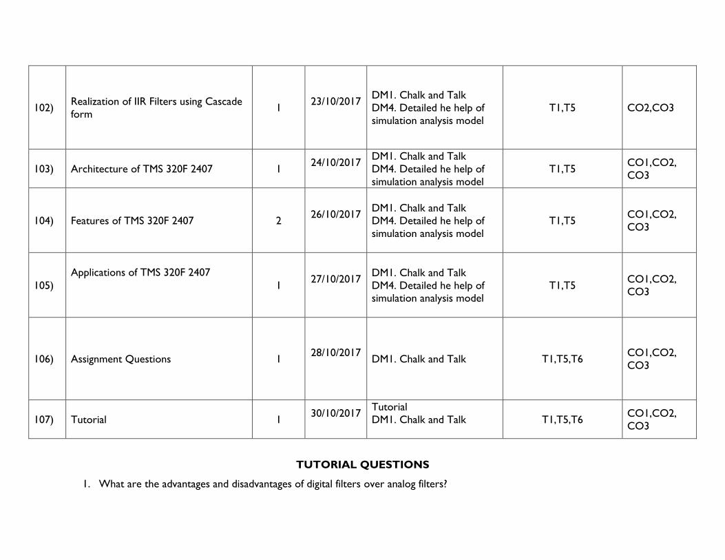
102) Realization of IIR Filters using Cascade
form 1
23/10/2017
DM1. Chalk and Talk
DM4. Detailed he help of
simulation analysis model
T1,T5 CO2,CO3
103) Architecture of TMS 320F 2407 1 24/10/2017
DM1. Chalk and Talk
DM4. Detailed he help of
simulation analysis model
T1,T5 CO1,CO2,
CO3
104) Features of TMS 320F 2407 2 26/10/2017
DM1. Chalk and Talk
DM4. Detailed he help of
simulation analysis model
T1,T5 CO1,CO2,
CO3
105)
Applications of TMS 320F 2407
1 27/10/2017
DM1. Chalk and Talk
DM4. Detailed he help of simulation analysis model
T1,T5 CO1,CO2, CO3
106) Assignment Questions 1 28/10/2017
DM1. Chalk and Talk
T1,T5,T6 CO1,CO2,
CO3
107) Tutorial 1 30/10/2017
Tutorial
DM1. Chalk and Talk
T1,T5,T6 CO1,CO2,
CO3
TUTORIAL QUESTIONS
1. What are the advantages and disadvantages of digital filters over analog filters?
2. Sketch and explain the frequency response of non ideal digital low pass filter
3. Consider the following specifications for a band pass filter Hd(ejω) ≤ 0.01 0 ≤ ω ≤ 0.2 π 0.92 ≤ Hd(ejω) ≤ 1.02
0.3π ≤ ω ≤ 0.7 π Hd(ejω) ≤ 0.02 0.8π ≤ ω ≤ π Design a linear phase FIR filter to meet these specifications using
Bartlett window.
4. With the help of illustrations explain zero interpolation, step interpolation and linear interpolation.
HOME ASSIGNMENT-V
Issue date: 23/09/2017 Submission date: 21/10/2017
1. Explain the FIR filter design using windowing technique.
2. Compare FIR and IIR filters.
3. Discuss the realization of FIR filter structures.
4. Discuss about characteristics linear phase FIR filters.
5. What are the effects of windowing?
6. Consider the following specifications for a band pass filter: Hd (ejω) ≤ 0.01 0 ≤ ω ≤ 0.2π 0.92 ≤ Hd (ejω) ≤ 1.02
0.3π ≤ ω ≤ 0.7π Hd (ejω) ≤ 0.02 0.8π ≤ ω ≤ π Design a linear phase FIR filter to meet these specifications using
Hamming window.
Assignment –I
Issue date: 19/08/2017 Submission date: 26/8/2017
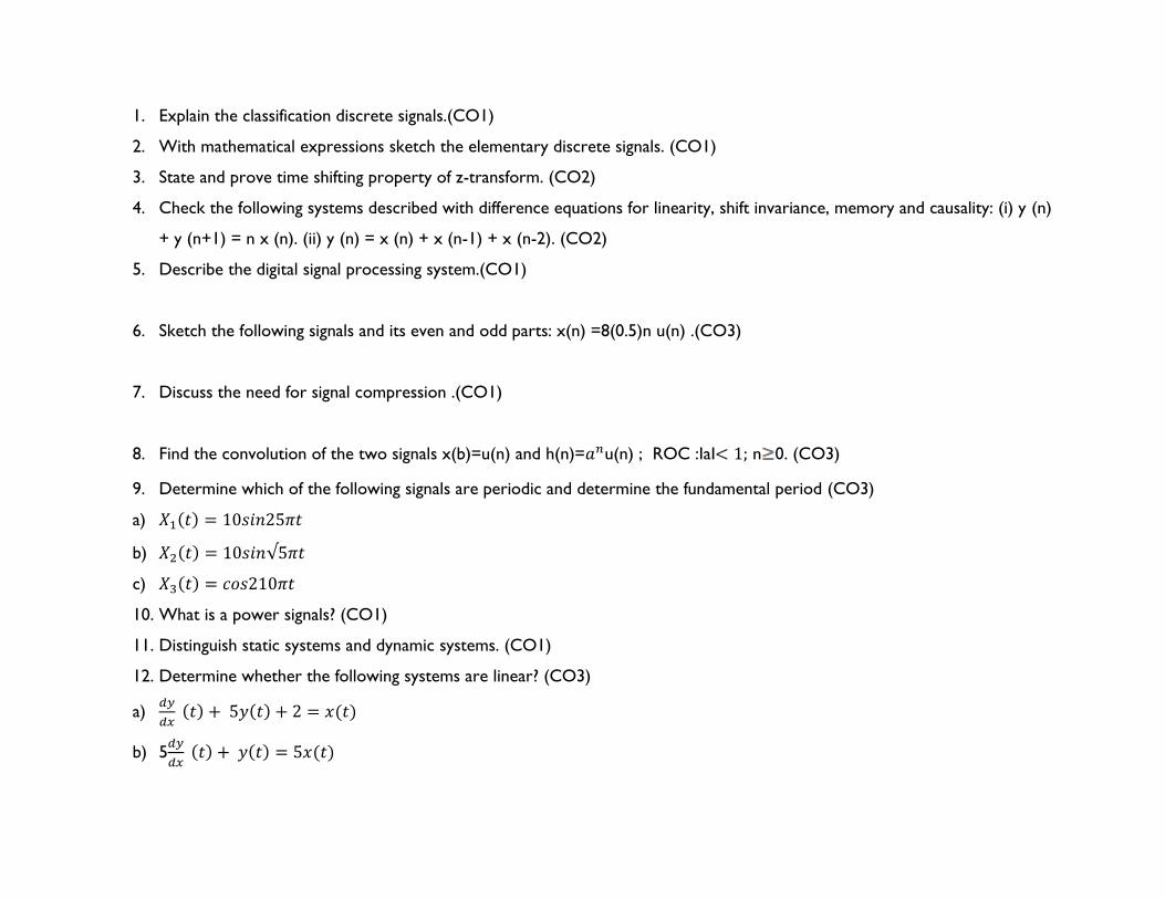
1. Explain the classification discrete signals.(CO1)
2. With mathematical expressions sketch the elementary discrete signals. (CO1)
3. State and prove time shifting property of z-transform. (CO2)
4. Check the following systems described with difference equations for linearity, shift invariance, memory and causality: (i) y (n)
+ y (n+1) = n x (n). (ii) y (n) = x (n) + x (n-1) + x (n-2). (CO2)
5. Describe the digital signal processing system.(CO1)
6. Sketch the following signals and its even and odd parts: x(n) =8(0.5)n u(n) .(CO3)
7. Discuss the need for signal compression .(CO1)
8. Find the convolution of the two signals x(b)=u(n) and h(n)=𝑎𝑛u(n) ; ROC :IaI< 1; n 0. (CO3)
9. Determine which of the following signals are periodic and determine the fundamental period (CO3)
a) 𝑋1(𝑡) = 10𝑠𝑖𝑛25𝜋𝑡
b) 𝑋2(𝑡) = 10𝑠𝑖𝑛√5𝜋𝑡
c) 𝑋3(𝑡) = 𝑐𝑜𝑠210𝜋𝑡
10. What is a power signals? (CO1)
11. Distinguish static systems and dynamic systems. (CO1)
12. Determine whether the following systems are linear? (CO3)
a) 𝑑𝑦
𝑑𝑥 (𝑡) + 5𝑦(𝑡) + 2 = 𝑥(𝑡)
b) 5𝑑𝑦
𝑑𝑥 (𝑡) + 𝑦(𝑡) = 5𝑥(𝑡)

13. What is BIBO Stability ? and what are the conditions for BIBO stability? (CO1)
14. What is meant by sampling? State the sampling theorem? (CO1)
15. Explain shift-invariant systems in detail? (CO1)
16. Distinguish between linear and circular convolutions method of two sequences. (CO1)
17. Define a DFT for a sequence x(n). (CO2)
18. State the properties of DFT? (CO1)
19. Obtain the DFT of the following sequence x(n)=72,-56,15,9.(CO2)
20. Develop a DITFFT algorithm for N=8 using a 4-point DFT and a 2 point DFT compare the number of multiplication with the
algorithm using only 2-point DFT’S. (CO2)
21. Find the DFT of the sample data sequence x (n) = 1, 1, 2, 2, 3, 3 and determine the corresponding amplitude and phase
spectrum. (CO2)
22. Discuss in detail the concept of decimation in time FFT. Also sketch the necessary flow graph for N=8. (CO3)
23. Discuss all types of symmetric properties of DFT. (CO1)
24. Draw the flow graph for 16-point radix–2 decimation in frequency FFT algorithm and explain it briefly. Also label the
multipliers appropriately. (CO2)
25. Given the two sequences of length ‘4’ as under x(n) = 1,2,3,1 h(n) = 4,3,2,2. Verify the answer using DFT method. (CO2)
26. Compare DIT-FFT and DIF-FFT algorithms. (CO1)
27. State and prove circular convolution property of DFT. (CO1)
28. Find DFT of sequence using DIT – FFT, the sequence is x (n) = 1, 1, 1, 1, 1, 1, 1, 1.(CO2)
29. Compute the 4-point DFT of the sequence x (n) = (1, 0, 1, 0) using DIF-FFT radix – 2 algorithm. Compare the answer with
conventional approach. (CO2)
30. Discuss the comparison between Fourier series and Fourier transform. (CO1)
12. MODEL QUESTION PAPER - I
VNR VIGNANA JYOTHI INSTITUTE OF ENGINEERING & TECHNOLOGY
(AN AUTONOMOUS INSTITUTE)
IV B.TECH. I SEMESTER REGULAR EXAMINATION-2017-18
SUBJECT: PRINCIPLES OF DIGITAL SIGNAL PROCESSING
(EEE)
Time: 3 Hours Max. Marks: 70
PART-A (compulsory) 30 marks
1. Answer in one sentence. [1 M]
a) Define symmetric and anti symmetric signals.
b) Define the Parseval’s Theorem
c) Explain the linearity property of z-transform.
d) Give any two properties of butter worth low pass filter.
e) What is Gibbs phenomenon?
Subject Code
13ECE083
R13
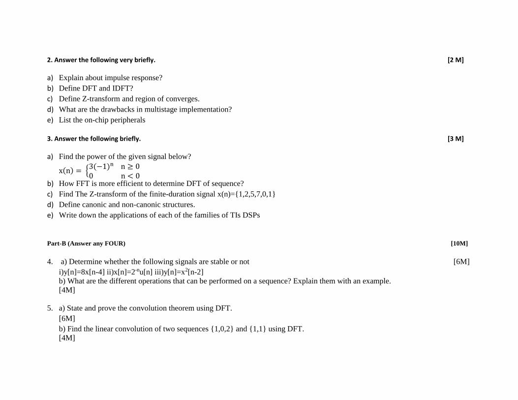
2. Answer the following very briefly. [2 M]
a) Explain about impulse response?
b) Define DFT and IDFT?
c) Define Z-transform and region of converges.
d) What are the drawbacks in multistage implementation?
e) List the on-chip peripherals
3. Answer the following briefly. [3 M]
a) Find the power of the given signal below?
x(n) = 3(−1)n n ≥ 00 n < 0
b) How FFT is more efficient to determine DFT of sequence?
c) Find The Z-transform of the finite-duration signal x(n)=1,2,5,7,0,1
d) Define canonic and non-canonic structures.
e) Write down the applications of each of the families of TIs DSPs
Part-B (Answer any FOUR) [10M]
4. a) Determine whether the following signals are stable or not [6M]
i)y[n]=8x[n-4] ii)x[n]=2-nu[n] iii)y[n]=x2[n-2]
b) What are the different operations that can be performed on a sequence? Explain them with an example.
[4M]
5. a) State and prove the convolution theorem using DFT.
[6M]
b) Find the linear convolution of two sequences 1,0,2 and 1,1 using DFT.
[4M]
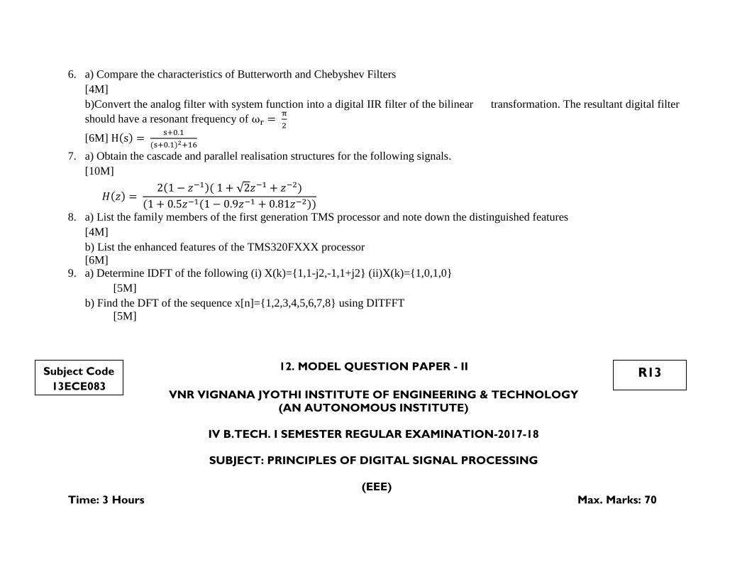
6. a) Compare the characteristics of Butterworth and Chebyshev Filters
[4M]
b)Convert the analog filter with system function into a digital IIR filter of the bilinear transformation. The resultant digital filter
should have a resonant frequency of ωr = π
2
[6M] H(s) = s+0.1
(s+0.1)2+16
7. a) Obtain the cascade and parallel realisation structures for the following signals.
[10M]
𝐻(𝑧) = 2(1 − 𝑧−1)( 1 + √2𝑧−1 + 𝑧−2)
(1 + 0.5𝑧−1(1 − 0.9𝑧−1 + 0.81𝑧−2))
8. a) List the family members of the first generation TMS processor and note down the distinguished features
[4M]
b) List the enhanced features of the TMS320FXXX processor
[6M]
9. a) Determine IDFT of the following (i) X(k)=1,1-j2,-1,1+j2 (ii)X(k)=1,0,1,0
[5M]
b) Find the DFT of the sequence x[n]=1,2,3,4,5,6,7,8 using DITFFT
[5M]
12. MODEL QUESTION PAPER - II
VNR VIGNANA JYOTHI INSTITUTE OF ENGINEERING & TECHNOLOGY
(AN AUTONOMOUS INSTITUTE)
IV B.TECH. I SEMESTER REGULAR EXAMINATION-2017-18
SUBJECT: PRINCIPLES OF DIGITAL SIGNAL PROCESSING
(EEE)
Time: 3 Hours Max. Marks: 70
Subject Code
13ECE083
R13
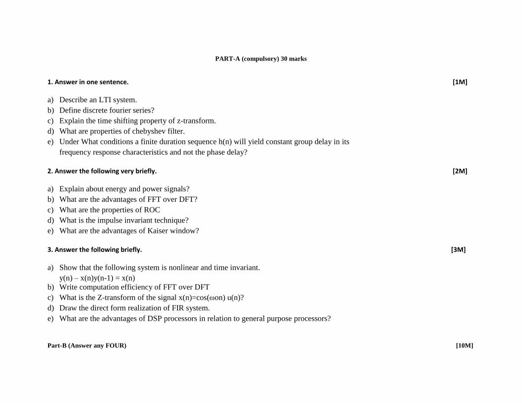
PART-A (compulsory) 30 marks
1. Answer in one sentence. [1M]
a) Describe an LTI system.
b) Define discrete fourier series?
c) Explain the time shifting property of z-transform.
d) What are properties of chebyshev filter.
e) Under What conditions a finite duration sequence h(n) will yield constant group delay in its
frequency response characteristics and not the phase delay?
2. Answer the following very briefly. [2M]
a) Explain about energy and power signals?
b) What are the advantages of FFT over DFT?
c) What are the properties of ROC
d) What is the impulse invariant technique?
e) What are the advantages of Kaiser window?
3. Answer the following briefly. [3M]
a) Show that the following system is nonlinear and time invariant.
y(n) – x(n)y(n-1) = x(n)
b) Write computation efficiency of FFT over DFT
c) What is the Z-transform of the signal x(n)=cos(ωon) u(n)?
d) Draw the direct form realization of FIR system.
e) What are the advantages of DSP processors in relation to general purpose processors?
Part-B (Answer any FOUR) [10M]
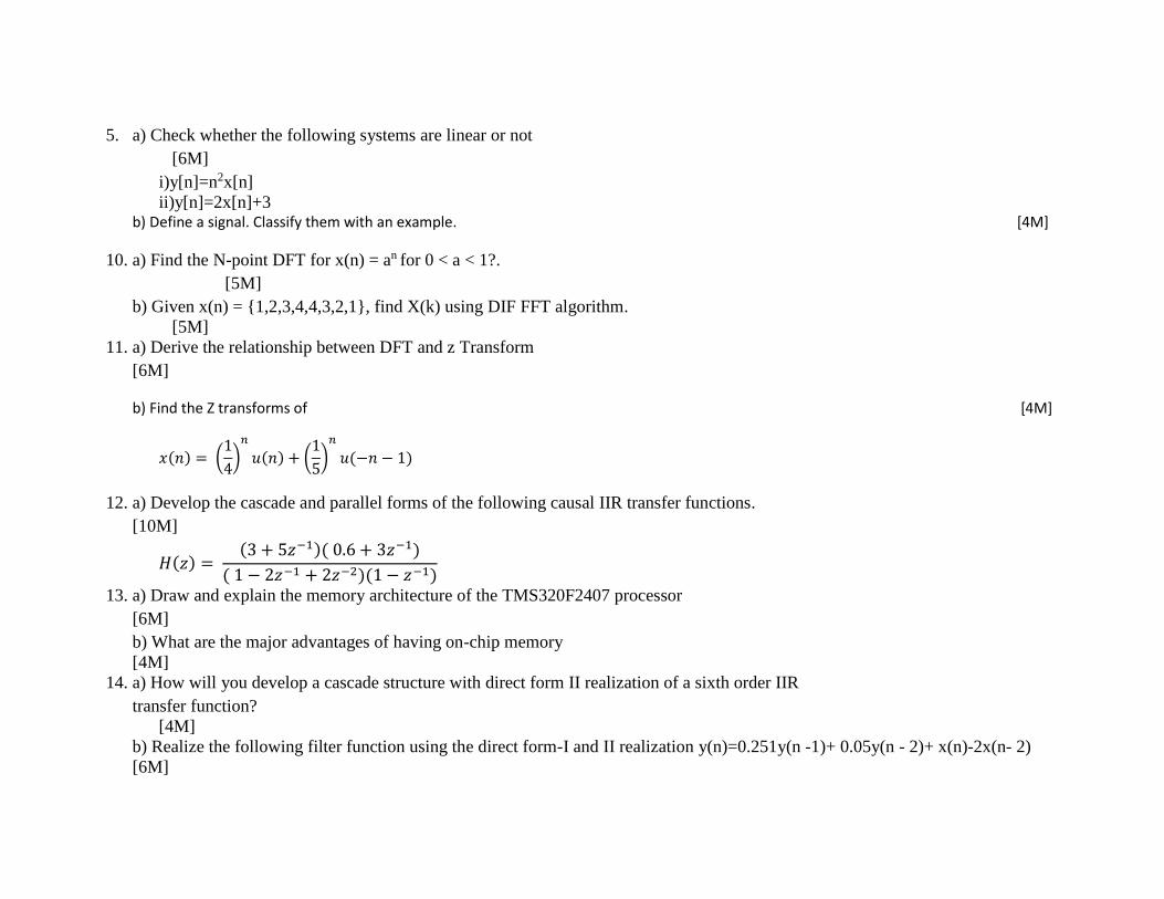
5. a) Check whether the following systems are linear or not
[6M]
i)y[n]=n2x[n]
ii)y[n]=2x[n]+3 b) Define a signal. Classify them with an example. [4M]
10. a) Find the N-point DFT for x(n) = an for 0 < a < 1?.
[5M]
b) Given x(n) = 1,2,3,4,4,3,2,1, find X(k) using DIF FFT algorithm.
[5M]
11. a) Derive the relationship between DFT and z Transform
[6M]
b) Find the Z transforms of [4M]
𝑥(𝑛) = (1
4)
𝑛
𝑢(𝑛) + (1
5)
𝑛
𝑢(−𝑛 − 1)
12. a) Develop the cascade and parallel forms of the following causal IIR transfer functions.
[10M]
𝐻(𝑧) = (3 + 5𝑧−1)( 0.6 + 3𝑧−1)
( 1 − 2𝑧−1 + 2𝑧−2)(1 − 𝑧−1)
13. a) Draw and explain the memory architecture of the TMS320F2407 processor
[6M]
b) What are the major advantages of having on-chip memory
[4M]
14. a) How will you develop a cascade structure with direct form II realization of a sixth order IIR
transfer function?
[4M]
b) Realize the following filter function using the direct form-I and II realization y(n)=0.251y(n -1)+ 0.05y(n - 2)+ x(n)-2x(n- 2)
[6M]
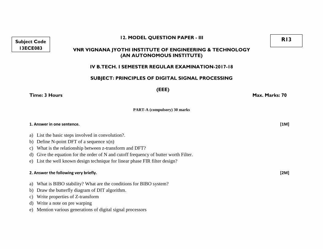
12. MODEL QUESTION PAPER - III
VNR VIGNANA JYOTHI INSTITUTE OF ENGINEERING & TECHNOLOGY
(AN AUTONOMOUS INSTITUTE)
IV B.TECH. I SEMESTER REGULAR EXAMINATION-2017-18
SUBJECT: PRINCIPLES OF DIGITAL SIGNAL PROCESSING
(EEE)
Time: 3 Hours Max. Marks: 70
PART-A (compulsory) 30 marks
1. Answer in one sentence. [1M]
a) List the basic steps involved in convolution?.
b) Define N-point DFT of a sequence x(n)
c) What is the relationship between z-transform and DFT?
d) Give the equation for the order of N and cutoff frequency of butter worth Filter.
e) List the well known design technique for linear phase FIR filter design?
2. Answer the following very briefly. [2M]
a) What is BIBO stability? What are the conditions for BIBO system?
b) Draw the butterfly diagram of DIT algorithm.
c) Write properties of Z-transform
d) Write a note on pre warping
e) Mention various generations of digital signal processors
Subject Code
13ECE083
R13
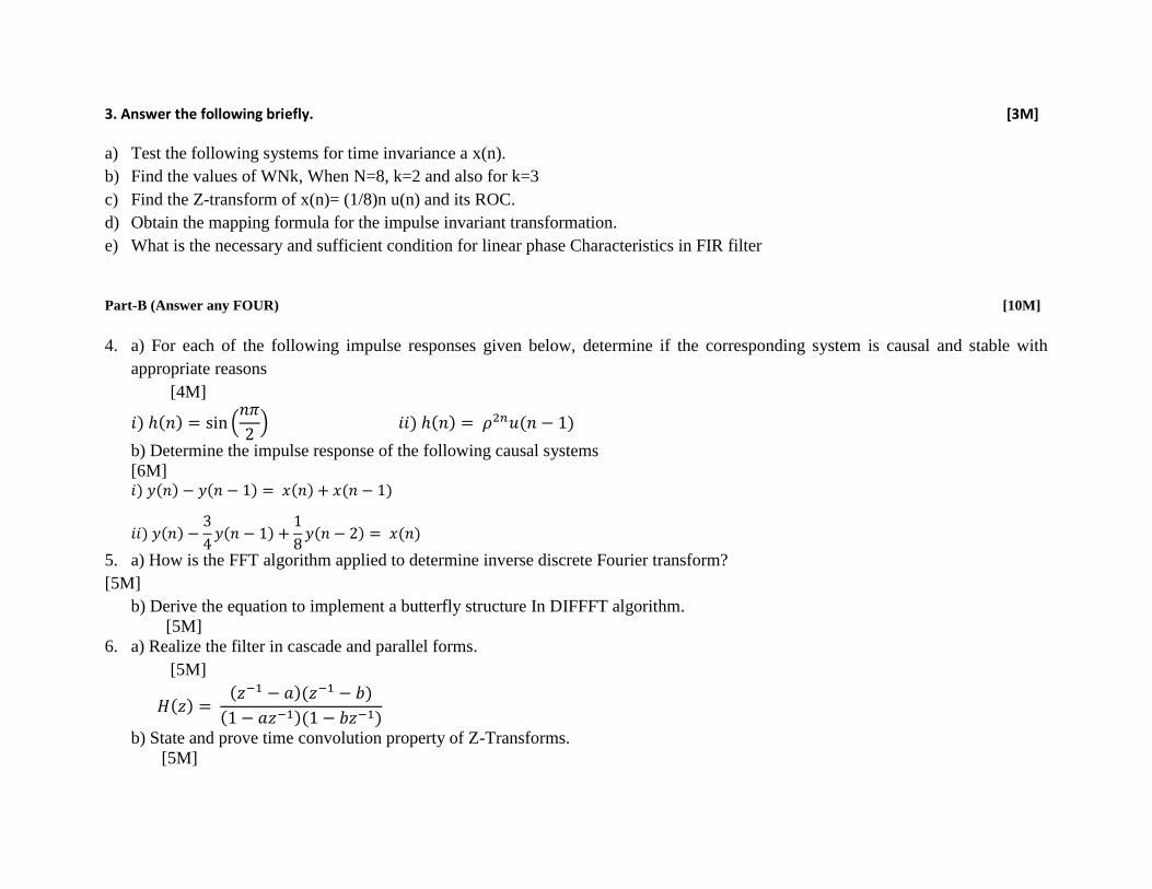
3. Answer the following briefly. [3M]
a) Test the following systems for time invariance a x(n).
b) Find the values of WNk, When N=8, k=2 and also for k=3
c) Find the Z-transform of x(n)= (1/8)n u(n) and its ROC.
d) Obtain the mapping formula for the impulse invariant transformation.
e) What is the necessary and sufficient condition for linear phase Characteristics in FIR filter
Part-B (Answer any FOUR) [10M]
4. a) For each of the following impulse responses given below, determine if the corresponding system is causal and stable with
appropriate reasons
[4M]
𝑖) ℎ(𝑛) = sin (𝑛𝜋
2) 𝑖𝑖) ℎ(𝑛) = 𝜌2𝑛𝑢(𝑛 − 1)
b) Determine the impulse response of the following causal systems
[6M] 𝑖) 𝑦(𝑛) − 𝑦(𝑛 − 1) = 𝑥(𝑛) + 𝑥(𝑛 − 1)
𝑖𝑖) 𝑦(𝑛) −3
4𝑦(𝑛 − 1) +
1
8𝑦(𝑛 − 2) = 𝑥(𝑛)
5. a) How is the FFT algorithm applied to determine inverse discrete Fourier transform?
[5M]
b) Derive the equation to implement a butterfly structure In DIFFFT algorithm.
[5M]
6. a) Realize the filter in cascade and parallel forms.
[5M]
𝐻(𝑧) = (𝑧−1 − 𝑎)(𝑧−1 − 𝑏)
(1 − 𝑎𝑧−1)(1 − 𝑏𝑧−1)
b) State and prove time convolution property of Z-Transforms.
[5M]
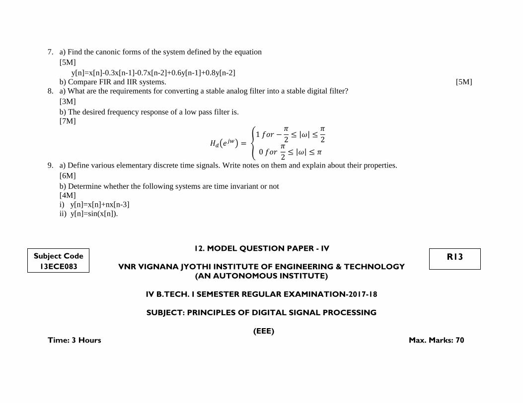
7. a) Find the canonic forms of the system defined by the equation
[5M]
y[n]=x[n]-0.3x[n-1]-0.7x[n-2]+0.6y[n-1]+0.8y[n-2]
b) Compare FIR and IIR systems. [5M]
8. a) What are the requirements for converting a stable analog filter into a stable digital filter?
[3M]
b) The desired frequency response of a low pass filter is.
[7M]
𝐻𝑑(𝑒𝑗𝑤) = 1 𝑓𝑜𝑟 −
𝜋
2≤ |𝜔| ≤
𝜋
2
0 𝑓𝑜𝑟 𝜋
2≤ |𝜔| ≤ 𝜋
9. a) Define various elementary discrete time signals. Write notes on them and explain about their properties.
[6M]
b) Determine whether the following systems are time invariant or not
[4M]
i) y[n]=x[n]+nx[n-3]
ii) y[n]=sin(x[n]).
12. MODEL QUESTION PAPER - IV
VNR VIGNANA JYOTHI INSTITUTE OF ENGINEERING & TECHNOLOGY
(AN AUTONOMOUS INSTITUTE)
IV B.TECH. I SEMESTER REGULAR EXAMINATION-2017-18
SUBJECT: PRINCIPLES OF DIGITAL SIGNAL PROCESSING
(EEE)
Time: 3 Hours Max. Marks: 70
Subject Code
13ECE083
R13
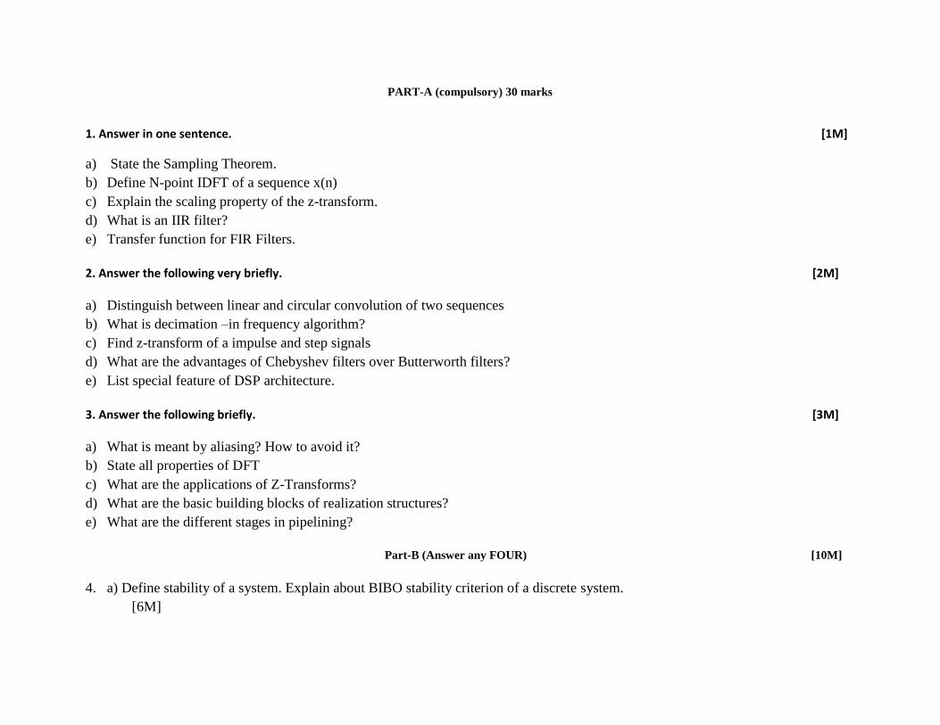
PART-A (compulsory) 30 marks
1. Answer in one sentence. [1M]
a) State the Sampling Theorem.
b) Define N-point IDFT of a sequence x(n)
c) Explain the scaling property of the z-transform.
d) What is an IIR filter?
e) Transfer function for FIR Filters.
2. Answer the following very briefly. [2M]
a) Distinguish between linear and circular convolution of two sequences
b) What is decimation –in frequency algorithm?
c) Find z-transform of a impulse and step signals
d) What are the advantages of Chebyshev filters over Butterworth filters?
e) List special feature of DSP architecture.
3. Answer the following briefly. [3M]
a) What is meant by aliasing? How to avoid it?
b) State all properties of DFT
c) What are the applications of Z-Transforms?
d) What are the basic building blocks of realization structures?
e) What are the different stages in pipelining?
Part-B (Answer any FOUR) [10M]
4. a) Define stability of a system. Explain about BIBO stability criterion of a discrete system.
[6M]

b) i)Draw the even and odd parts of the following signals x[n]=5,4,3,2,1 ii)Check u[n]-u[n-6] is a power signal or not
[4M]
5. a) Find the DFT of the sequence x[n]=1,2,3,4,5,6,7,8.
[5M]
b) Explain the use of FFT algorithms in linear filtering and correlation. [5M]
6. a) Find out the Z-transform for the following discrete time sequence x(n) = kn, n 0
[5M]
b) Explain how the analysis of discrete time invariant system can be obtained by using convolution properties of the Z-
Transform? [5M]
7. a) Realize the following IIR system functions in the direct form I and II and also parallel form
[10M]
𝐻(𝑧) = 1
(1 − 𝑎𝑧−1)2+
1
(1 − 𝑏𝑧−1)2
8. a) What is MAC? Explain its operation in detail [7M]
b) What are the various addressing modes used in the TMS320F2407 processor?
[3M]
9. a) Determine whether the following systems are stable, casual, linear and time-invariant
[6M]
𝑖) 𝑇(𝑥(𝑛)) = 𝑔(𝑛)𝑥(𝑛)
𝑖𝑖) 𝑇(𝑥(𝑛)) = ∑ 𝑥(𝑘)
𝑛
𝑘=𝑛0
b) Determine the impulse response of the following causal systems
[4M] 𝑖) 𝑦(𝑛) − 2 𝑐𝑜𝑠𝜃𝑦(𝑛 − 2) + 𝑦(𝑛 − 2) = 𝑥(𝑛)
𝑖𝑖) 𝑦(𝑛) − 3𝑦(𝑛 − 1) + 2𝑦(𝑛 − 2) = 𝑥(𝑛) + 3𝑥(𝑛 − 1) + 2𝑥(𝑛 − 2)
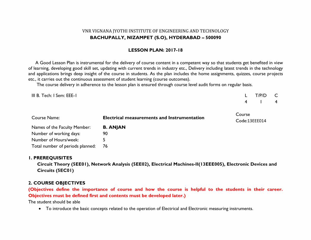
VNR VIGNANA JYOTHI INSTITUTE OF ENGINEERING AND TECHNOLOGY
BACHUPALLY, NIZAMPET (S.O), HYDERABAD – 500090
LESSON PLAN: 2017-18
A Good Lesson Plan is instrumental for the delivery of course content in a competent way so that students get benefited in view
of learning, developing good skill set, updating with current trends in industry etc., Delivery including latest trends in the technology
and applications brings deep insight of the course in students. As the plan includes the home assignments, quizzes, course projects
etc., it carries out the continuous assessment of student learning (course outcomes).
The course delivery in adherence to the lesson plan is ensured through course level audit forms on regular basis.
III B. Tech: I Sem: EEE-1 L T/P/D C
4 1 4
Course Name: Electrical measurements and Instrumentation Course
Code:13EEE014
Names of the Faculty Member: B. ANJAN
Number of working days: 90
Number of Hours/week: 5
Total number of periods planned: 76
1. PREREQUISITES
Circuit Theory (5EE01), Network Analysis (5EE02), Electrical Machines-II(13EEE005), Electronic Devices and
Circuits (5EC01)
2. COURSE OBJECTIVES
(Objectives define the importance of course and how the course is helpful to the students in their career.
Objectives must be defined first and contents must be developed later.)
The student should be able
• To introduce the basic concepts related to the operation of Electrical and Electronic measuring instruments.
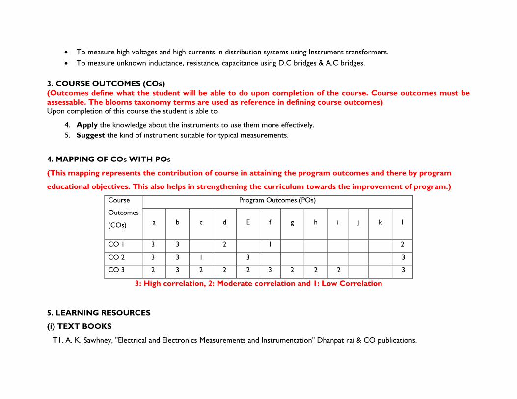
• To measure high voltages and high currents in distribution systems using Instrument transformers.
• To measure unknown inductance, resistance, capacitance using D.C bridges & A.C bridges.
3. COURSE OUTCOMES (COs)
(Outcomes define what the student will be able to do upon completion of the course. Course outcomes must be
assessable. The blooms taxonomy terms are used as reference in defining course outcomes)
Upon completion of this course the student is able to
4. Apply the knowledge about the instruments to use them more effectively.
5. Suggest the kind of instrument suitable for typical measurements.
4. MAPPING OF COs WITH POs
(This mapping represents the contribution of course in attaining the program outcomes and there by program
educational objectives. This also helps in strengthening the curriculum towards the improvement of program.)
Course
Outcomes
(COs)
Program Outcomes (POs)
a b c d E f g h i j k l
CO 1 3 3 2 1 2
CO 2 3 3 1 3 3
CO 3 2 3 2 2 2 3 2 2 2 3
3: High correlation, 2: Moderate correlation and 1: Low Correlation
5. LEARNING RESOURCES
(i) TEXT BOOKS
T1. A. K. Sawhney, "Electrical and Electronics Measurements and Instrumentation" Dhanpat rai & CO publications.

T2. Golding, E.W, Sir Issac Pitman and Sons, "Electrical Measurement and Measuring Instruments" , (IIIrd Edition), 1960.
T3. Helfrick, Albert D, Cooper William, “Modern Electronic Instrumentation and Measurement Techniques” DPrentice-Hall of
India, Reprint 1992.
(ii) REFERENCES (Publications/ Open Learning Resources)
(Course delivery including latest trends brings good insight of the course in students and also inculcates the habit of
self learning among the students.
Publications referred can be given unit wise or at course level.)
(b) Open Learning Resources for self learning
L1. http://nptel.ac.in/courses/108105053/43
L2. ieee-ims.org
(iii) JOURNALS
J1. IEEE Transactions on Instrumentation and Measurement
J2. IEEE Instrumentation & Measurement Magazine
6. DELIVERY METHODOLOGIES
(Depending on the suitability to the delivery of concept, one or more among the following delivery methodologies
are adopted to engage the student in learning)
DM1: Chalk and Talk DM5: Open The Box
DM3: Collaborative Learning (Think Pair Share, POGIL, etc.) DM7: Group Project
DM4: Demonstration (Physical / Laboratory / Audio Visuals)
7. PROPOSED FIELD VISITS/ GUEST LECTURE BY INDUSTRY EXPERT
(To be added for the courses as directed by the department.)
8. ASSESSMENT
(As per Regulations, AM1 and AM2 are compulsory for assessment. Whereas, any two or more assessment
methodologies can be considered from AM3 to AM9 under assignment towards continuous assessment of the
performance of students.)
AM1: Semester End Examination . AM2: Mid Term Examination
AM3: Home Assignments
AM6: Quizzes
AM7: Course Projects**
** (To be added for the courses as directed by the department. The no. of course projects is left to the liberty of
faculty)
9. WEIGHTAGES FOR PROPOSED ASSESSMENT METHODOLOGIES
(The allotted marks for home assignments, quizzes etc., except course projects are left to the liberty of faculty.
But for the finalisation of assignment marks, the following weightages can be considered.)
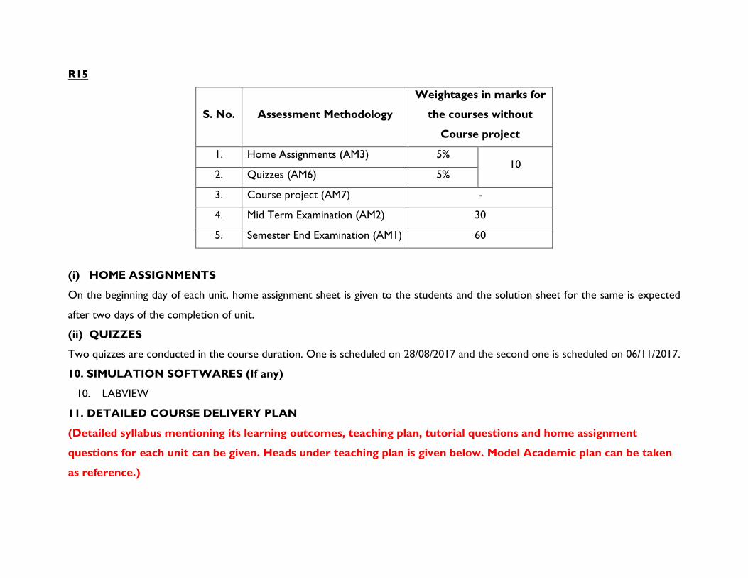
R15
S. No. Assessment Methodology
Weightages in marks for
the courses without
Course project
1. Home Assignments (AM3) 5% 10
2. Quizzes (AM6) 5%
3. Course project (AM7) -
4. Mid Term Examination (AM2) 30
5. Semester End Examination (AM1) 60
(i) HOME ASSIGNMENTS
On the beginning day of each unit, home assignment sheet is given to the students and the solution sheet for the same is expected
after two days of the completion of unit.
(ii) QUIZZES
Two quizzes are conducted in the course duration. One is scheduled on 28/08/2017 and the second one is scheduled on 06/11/2017.
10. SIMULATION SOFTWARES (If any)
10. LABVIEW
11. DETAILED COURSE DELIVERY PLAN
(Detailed syllabus mentioning its learning outcomes, teaching plan, tutorial questions and home assignment
questions for each unit can be given. Heads under teaching plan is given below. Model Academic plan can be taken
as reference.)
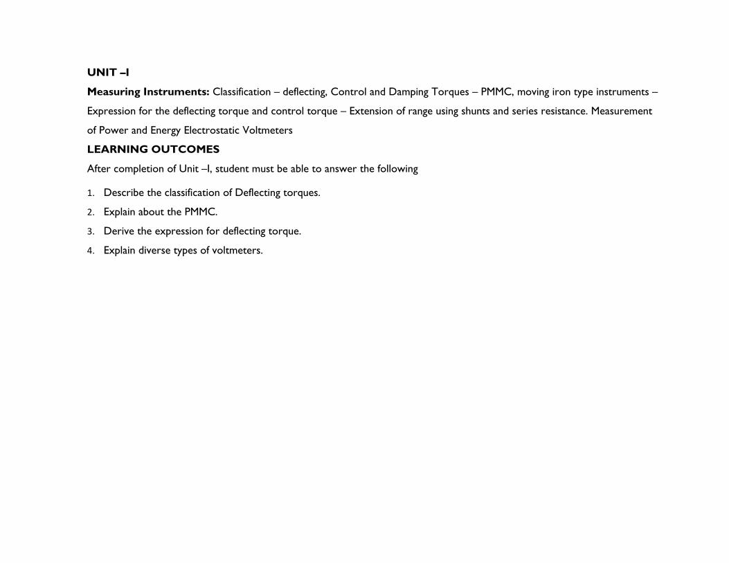
UNIT –I
Measuring Instruments: Classification – deflecting, Control and Damping Torques – PMMC, moving iron type instruments –
Expression for the deflecting torque and control torque – Extension of range using shunts and series resistance. Measurement
of Power and Energy Electrostatic Voltmeters
LEARNING OUTCOMES
After completion of Unit –I, student must be able to answer the following
1. Describe the classification of Deflecting torques.
2. Explain about the PMMC.
3. Derive the expression for deflecting torque.
4. Explain diverse types of voltmeters.

TEACHING PLAN
S.
No. Contents of syllabus to be taught
No. of
Lecture
Periods
Lecture
Dates
Proposed Delivery
Methodologies
Learning Resources /
References
(Text Books /
Journals /
Publications/ Open
Learning Resources)
Course
Outcomes
108)
Introduction to measurements:
1. Classification of methods of
measurement
2. Classification of measuring
instruments
3. Accuracy, precision, Reproducibility
1 04-07-17
DM1. Chalk and Talk (along
with PPT)
L.1.
T.1& T.2
CO 1 & CO2
109)
Mechanism to produce
Deflection Torque
Controlling Torque
Damping Torque
1 06-07-17 DM1. Chalk and Talk
T.1 & T.2 CO 1 & CO2
110)
PMMC Instrument
Equation for deflection torque
Errors and compensation
Swaping resistance
2 07-07-17
DM1. Chalk and Talk (along
with PPT)
T.1 & T.2 CO 1 & CO2
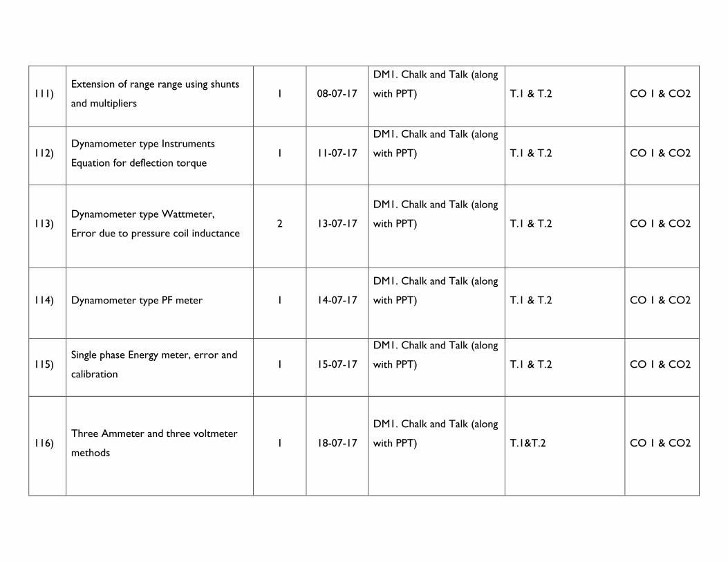
111) Extension of range range using shunts
and multipliers 1 08-07-17
DM1. Chalk and Talk (along
with PPT)
T.1 & T.2 CO 1 & CO2
112) Dynamometer type Instruments
Equation for deflection torque 1 11-07-17
DM1. Chalk and Talk (along
with PPT)
T.1 & T.2 CO 1 & CO2
113) Dynamometer type Wattmeter,
Error due to pressure coil inductance 2 13-07-17
DM1. Chalk and Talk (along
with PPT)
T.1 & T.2 CO 1 & CO2
114) Dynamometer type PF meter 1 14-07-17
DM1. Chalk and Talk (along
with PPT)
T.1 & T.2 CO 1 & CO2
115) Single phase Energy meter, error and
calibration 1 15-07-17
DM1. Chalk and Talk (along
with PPT)
T.1 & T.2 CO 1 & CO2
116) Three Ammeter and three voltmeter
methods 1 18-07-17
DM1. Chalk and Talk (along
with PPT)
T.1&T.2 CO 1 & CO2

117) Numerical Problems
1 20/07/17 Tutorial T.1&T.2 CO 1 & CO2
118) Electrostatic voltmeters 1 21/07/17
DM1. Chalk and Talk (along
with PPT)
T.1&T.2 CO 1 & CO2
UNIT- II
Measurement of resistance, Inductance and capacitance: Method of measuring low, medium and high resistance,
insulation resistance measurements, AC bridges for Inductance and capacitance Measurement, Merge
LEARNING OUTCOMES
After completion of this unit the student will be able to
4. Measure inductance, Capacitance, quality factor and dissipation factor by A.C. bridges.
5. To measure and differentiate low, medium, and high resistance measurements.
6. Measure insulation resistance

TEACHING PLAN
S.
No. Contents of syllabus to be taught
No. of
Lecture
Periods
Lecture
Dates
Proposed Delivery
Methodologies
Learning Resources /
References
(Text Books /
Journals /
Publications/ Open
Learning Resources)
Course
Outcomes
1)
Classification of resistance
Measurement of low resistance by
Kelvin’s double bridge
Medium and high resistance
measurements
03 22-07-17
25-07-17
DM1. Chalk and Talk (along
with PPT)
DM4. Demonstration of
one example.
L.1.
T.1& T.2
CO 1 & CO 2
2) Measurement of Inductance and quality
factor 04
27-07-17
28-07-17
29-07-17
DM1. Chalk and Talk
DM4. Detailed analysis with
the help of laboratory
experiment.
T.1& T.2 CO 1 & CO 2
3) Numerical problems 02
01-08-17
03-08-17
Tutorial T.1 & T.2 CO 1 & CO 2
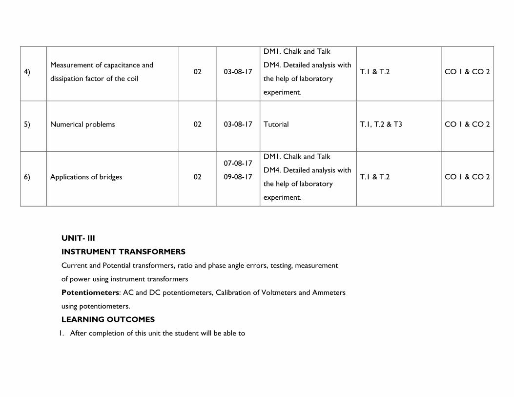
4) Measurement of capacitance and
dissipation factor of the coil 02 03-08-17
DM1. Chalk and Talk
DM4. Detailed analysis with
the help of laboratory
experiment.
T.1 & T.2 CO 1 & CO 2
5) Numerical problems 02 03-08-17 Tutorial T.1, T.2 & T3 CO 1 & CO 2
6) Applications of bridges 02
07-08-17
09-08-17
DM1. Chalk and Talk
DM4. Detailed analysis with
the help of laboratory
experiment.
T.1 & T.2 CO 1 & CO 2
UNIT- III
INSTRUMENT TRANSFORMERS
Current and Potential transformers, ratio and phase angle errors, testing, measurement
of power using instrument transformers
Potentiometers: AC and DC potentiometers, Calibration of Voltmeters and Ammeters
using potentiometers.
LEARNING OUTCOMES
1. After completion of this unit the student will be able to
2. Explain the principle and operation of D.C Crompton’s potentiometer.
3. Explain about the standardization process.
4. Explain about A.C Potentiometer.
5. Differentiate power transformers and instrumental transformers & their applications.
6. Measure power using instrumental transformers.

TEACHING PLAN
S.
No. Contents of syllabus to be taught
No. of
Lecture
Periods
Lecture
Dates
Proposed Delivery
Methodologies
Learning Resources /
References
(Text Books /
Journals /
Publications/ Open
Learning Resources)
Course
Outcomes
1) Introduction to Instrumental
transformers 2 10-08-17
DM1. Chalk and Talk (along
with PPT)
T.1& T.2 CO 1 & CO 2
2) CT’s 03
11-08-17
12-08-17
16-08-17
DM1. Chalk and Talk
DM4. Detailed analysis with
the help of laboratory
experiment.
T.1& T.2 CO 1 & CO 2
3) Numerical problems 3 17-08-17
18-08-17 Tutorial T.1 & T.2 CO 1 & CO 2
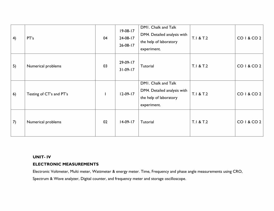
4) PT’s 04
19-08-17
24-08-17
26-08-17
DM1. Chalk and Talk
DM4. Detailed analysis with
the help of laboratory
experiment.
T.1 & T.2 CO 1 & CO 2
5) Numerical problems 03 29-09-17
31-09-17 Tutorial T.1 & T.2 CO 1 & CO 2
6) Testing of CT’s and PT’s 1 12-09-17
DM1. Chalk and Talk
DM4. Detailed analysis with
the help of laboratory
experiment.
T.1 & T.2 CO 1 & CO 2
7) Numerical problems 02 14-09-17 Tutorial T.1 & T.2 CO 1 & CO 2
UNIT- IV
ELECTRONIC MEASUREMENTS
Electronic Voltmeter, Multi meter, Wattmeter & energy meter. Time, Frequency and phase angle measurements using CRO,
Spectrum & Wave analyzer, Digital counter, and frequency meter and storage oscilloscope.
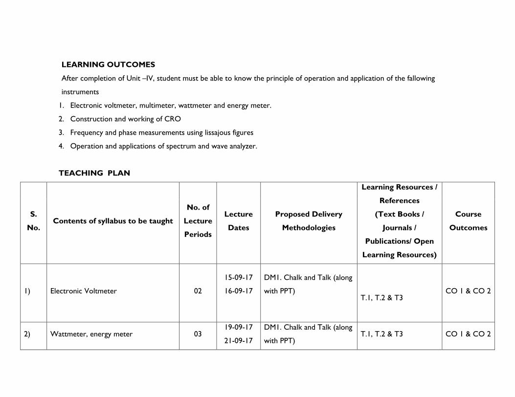
LEARNING OUTCOMES
After completion of Unit –IV, student must be able to know the principle of operation and application of the fallowing
instruments
1. Electronic voltmeter, multimeter, wattmeter and energy meter.
2. Construction and working of CRO
3. Frequency and phase measurements using lissajous figures
4. Operation and applications of spectrum and wave analyzer.
TEACHING PLAN
S.
No. Contents of syllabus to be taught
No. of
Lecture
Periods
Lecture
Dates
Proposed Delivery
Methodologies
Learning Resources /
References
(Text Books /
Journals /
Publications/ Open
Learning Resources)
Course
Outcomes
1) Electronic Voltmeter 02
15-09-17
16-09-17
DM1. Chalk and Talk (along
with PPT)
T.1, T.2 & T3 CO 1 & CO 2
2) Wattmeter, energy meter 03 19-09-17
21-09-17
DM1. Chalk and Talk (along
with PPT) T.1, T.2 & T3 CO 1 & CO 2
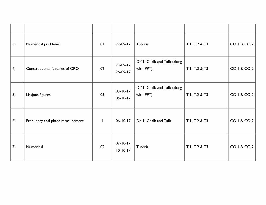
3) Numerical problems 01 22-09-17 Tutorial T.1, T.2 & T3 CO 1 & CO 2
4) Constructional features of CRO 02 23-09-17
26-09-17
DM1. Chalk and Talk (along
with PPT)
T.1, T.2 & T3 CO 1 & CO 2
5) Lissjous figures 03 03-10-17
05-10-17
DM1. Chalk and Talk (along
with PPT)
T.1, T.2 & T3 CO 1 & CO 2
6) Frequency and phase measurement I 06-10-17 DM1. Chalk and Talk T.1, T.2 & T3 CO 1 & CO 2
7) Numerical 02 07-10-17
10-10-17 Tutorial T.1, T.2 & T3 CO 1 & CO 2
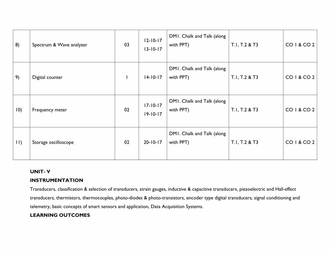
8) Spectrum & Wave analyzer 03 12-10-17
13-10-17
DM1. Chalk and Talk (along
with PPT)
T.1, T.2 & T3 CO 1 & CO 2
9) Digital counter 1 14-10-17
DM1. Chalk and Talk (along
with PPT)
T.1, T.2 & T3 CO 1 & CO 2
10) Frequency meter 02 17-10-17
19-10-17
DM1. Chalk and Talk (along
with PPT)
T.1, T.2 & T3 CO 1 & CO 2
11) Storage oscilloscope 02 20-10-17
DM1. Chalk and Talk (along
with PPT)
T.1, T.2 & T3 CO 1 & CO 2
UNIT- V
INSTRUMENTATION
Transducers, classification & selection of transducers, strain gauges, inductive & capacitive transducers, piezoelectric and Hall-effect
transducers, thermistors, thermocouples, photo-diodes & photo-transistors, encoder type digital transducers, signal conditioning and
telemetry, basic concepts of smart sensors and application, Data Acquisition Systems.
LEARNING OUTCOMES
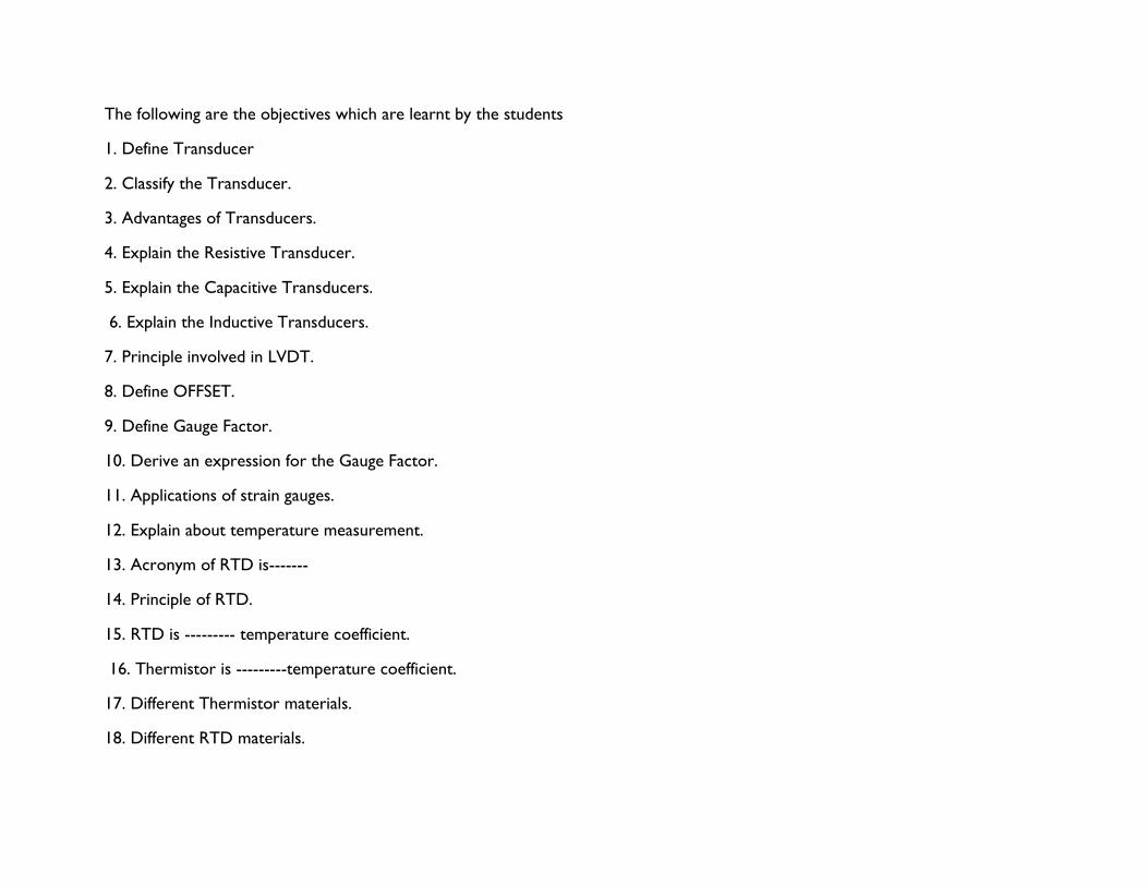
The following are the objectives which are learnt by the students
1. Define Transducer
2. Classify the Transducer.
3. Advantages of Transducers.
4. Explain the Resistive Transducer.
5. Explain the Capacitive Transducers.
6. Explain the Inductive Transducers.
7. Principle involved in LVDT.
8. Define OFFSET.
9. Define Gauge Factor.
10. Derive an expression for the Gauge Factor.
11. Applications of strain gauges.
12. Explain about temperature measurement.
13. Acronym of RTD is-------
14. Principle of RTD.
15. RTD is --------- temperature coefficient.
16. Thermistor is ---------temperature coefficient.
17. Different Thermistor materials.
18. Different RTD materials.
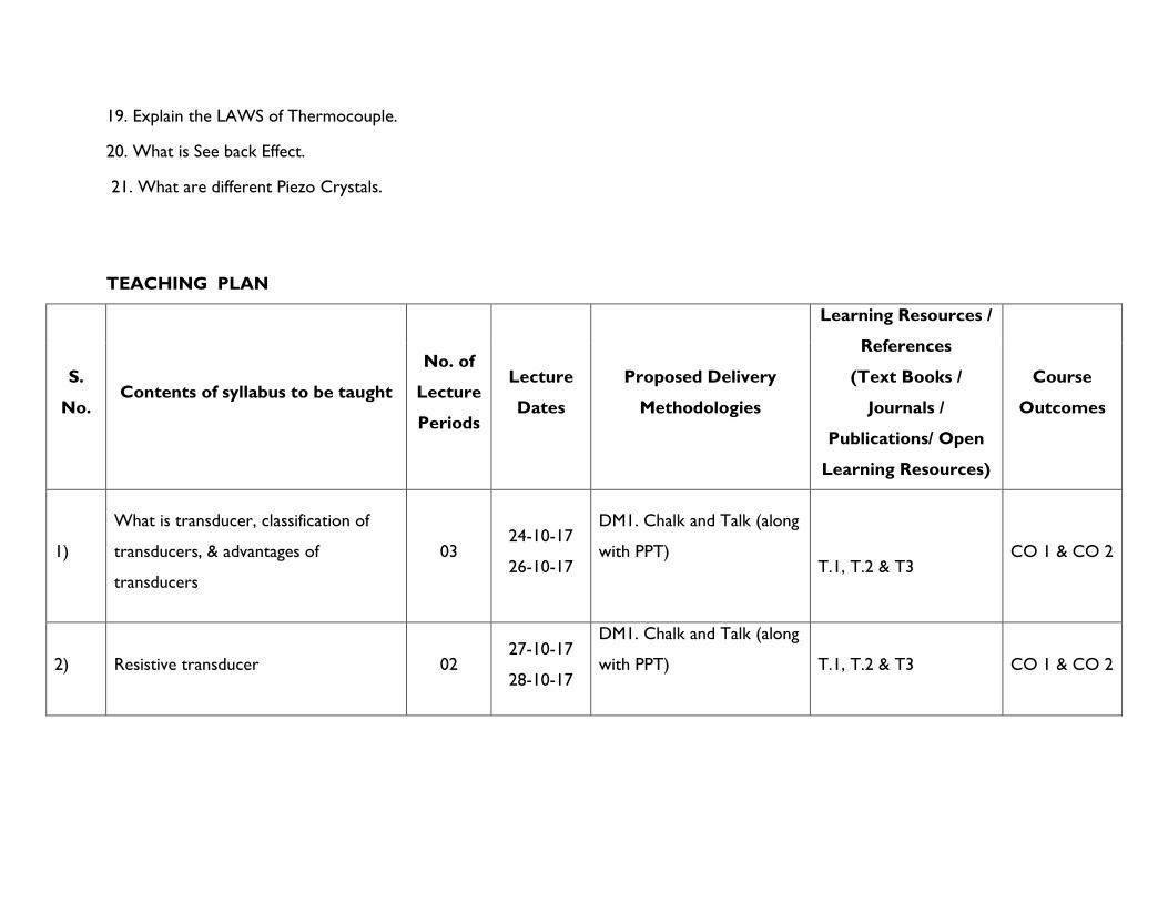
19. Explain the LAWS of Thermocouple.
20. What is See back Effect.
21. What are different Piezo Crystals.
TEACHING PLAN
S.
No. Contents of syllabus to be taught
No. of
Lecture
Periods
Lecture
Dates
Proposed Delivery
Methodologies
Learning Resources /
References
(Text Books /
Journals /
Publications/ Open
Learning Resources)
Course
Outcomes
1)
What is transducer, classification of
transducers, & advantages of
transducers
03 24-10-17
26-10-17
DM1. Chalk and Talk (along
with PPT)
T.1, T.2 & T3 CO 1 & CO 2
2) Resistive transducer 02 27-10-17
28-10-17
DM1. Chalk and Talk (along
with PPT)
T.1, T.2 & T3 CO 1 & CO 2
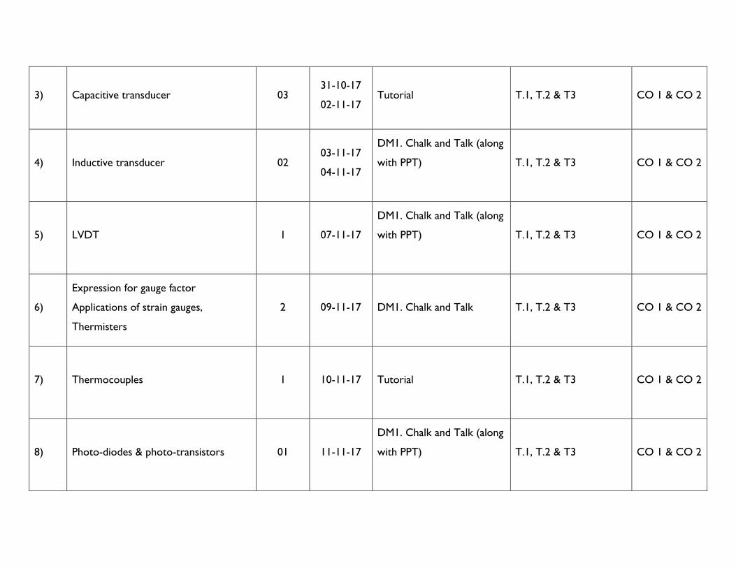
3) Capacitive transducer 03 31-10-17
02-11-17 Tutorial T.1, T.2 & T3 CO 1 & CO 2
4) Inductive transducer 02 03-11-17
04-11-17
DM1. Chalk and Talk (along
with PPT)
T.1, T.2 & T3 CO 1 & CO 2
5) LVDT 1 07-11-17
DM1. Chalk and Talk (along
with PPT)
T.1, T.2 & T3 CO 1 & CO 2
6)
Expression for gauge factor
Applications of strain gauges,
Thermisters
2 09-11-17 DM1. Chalk and Talk T.1, T.2 & T3 CO 1 & CO 2
7) Thermocouples 1 10-11-17 Tutorial T.1, T.2 & T3 CO 1 & CO 2
8) Photo-diodes & photo-transistors 01 11-11-17
DM1. Chalk and Talk (along
with PPT)
T.1, T.2 & T3 CO 1 & CO 2
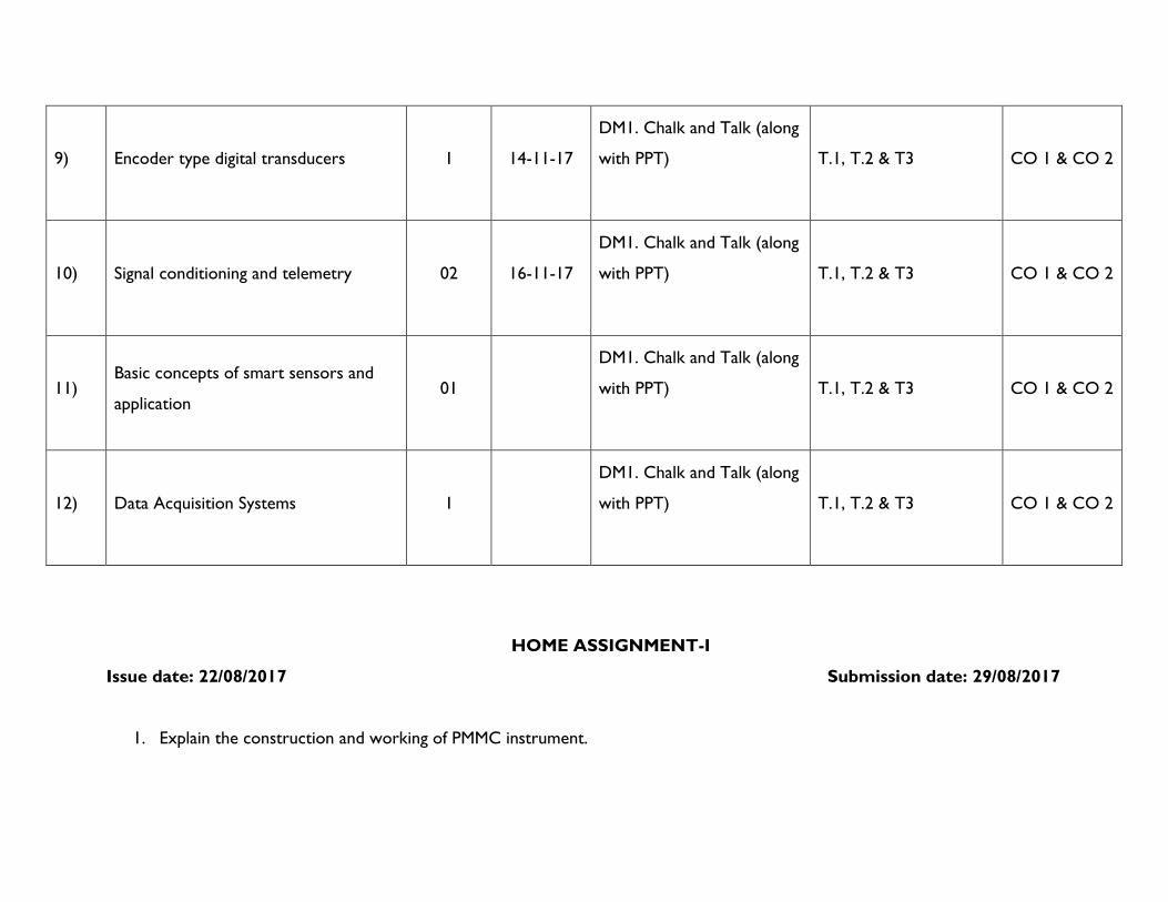
9) Encoder type digital transducers 1 14-11-17
DM1. Chalk and Talk (along
with PPT)
T.1, T.2 & T3 CO 1 & CO 2
10) Signal conditioning and telemetry 02 16-11-17
DM1. Chalk and Talk (along
with PPT)
T.1, T.2 & T3 CO 1 & CO 2
11) Basic concepts of smart sensors and
application 01
DM1. Chalk and Talk (along
with PPT)
T.1, T.2 & T3 CO 1 & CO 2
12) Data Acquisition Systems 1
DM1. Chalk and Talk (along
with PPT)
T.1, T.2 & T3 CO 1 & CO 2
HOME ASSIGNMENT-I
Issue date: 22/08/2017 Submission date: 29/08/2017
1. Explain the construction and working of PMMC instrument.
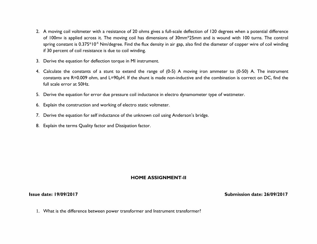
2. A moving coil voltmeter with a resistance of 20 ohms gives a full-scale deflection of 120 degrees when a potential difference
of 100mv is applied across it. The moving coil has dimensions of 30mm*25mm and is wound with 100 turns. The control
spring constant is 0.375*10-6 Nm/degree. Find the flux density in air gap, also find the diameter of copper wire of coil winding
if 30 percent of coil resistance is due to coil winding.
3. Derive the equation for deflection torque in MI instrument.
4. Calculate the constants of a stunt to extend the range of (0-5) A moving iron ammeter to (0-50) A. The instrument
constants are R=0.009 ohm, and L=90µH. If the shunt is made non-inductive and the combination is correct on DC, find the
full scale error at 50Hz.
5. Derive the equation for error due pressure coil inductance in electro dynamometer type of wattmeter.
6. Explain the construction and working of electro static voltmeter.
7. Derive the equation for self inductance of the unknown coil using Anderson’s bridge.
8. Explain the terms Quality factor and Dissipation factor.
HOME ASSIGNMENT-II
Issue date: 19/09/2017 Submission date: 26/09/2017
1. What is the difference between power transformer and Instrument transformer?
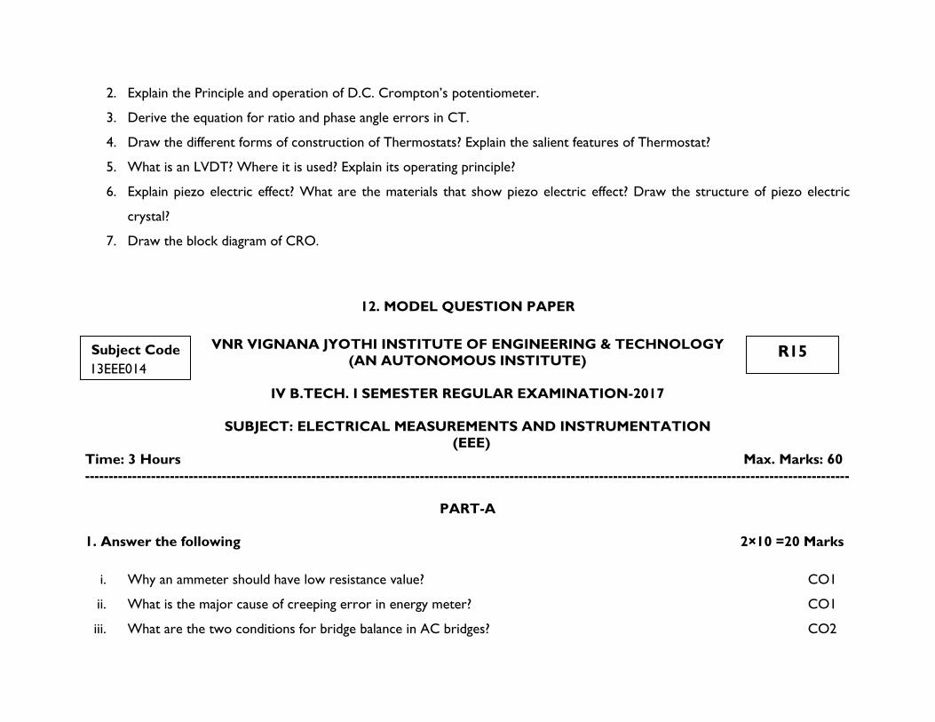
2. Explain the Principle and operation of D.C. Crompton’s potentiometer.
3. Derive the equation for ratio and phase angle errors in CT.
4. Draw the different forms of construction of Thermostats? Explain the salient features of Thermostat?
5. What is an LVDT? Where it is used? Explain its operating principle?
6. Explain piezo electric effect? What are the materials that show piezo electric effect? Draw the structure of piezo electric
crystal?
7. Draw the block diagram of CRO.
12. MODEL QUESTION PAPER
VNR VIGNANA JYOTHI INSTITUTE OF ENGINEERING & TECHNOLOGY
(AN AUTONOMOUS INSTITUTE)
IV B.TECH. I SEMESTER REGULAR EXAMINATION-2017
SUBJECT: ELECTRICAL MEASUREMENTS AND INSTRUMENTATION
(EEE)
Time: 3 Hours Max. Marks: 60
------------------------------------------------------------------------------------------------------------------------------------------------------------------
PART-A
1. Answer the following 2×10 =20 Marks
i. Why an ammeter should have low resistance value? CO1
ii. What is the major cause of creeping error in energy meter? CO1
iii. What are the two conditions for bridge balance in AC bridges? CO2
Subject Code
13EEE014
R15
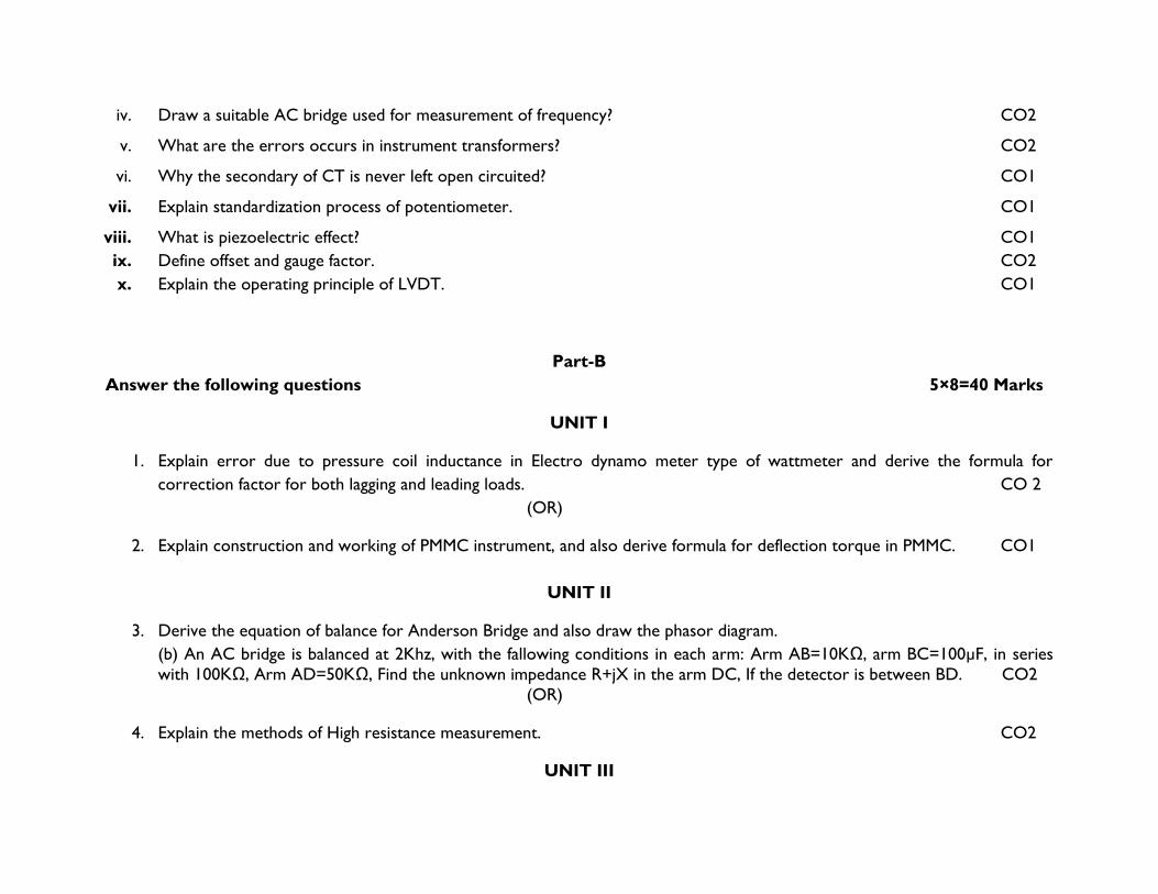
iv. Draw a suitable AC bridge used for measurement of frequency? CO2
v. What are the errors occurs in instrument transformers? CO2
vi. Why the secondary of CT is never left open circuited? CO1
vii. Explain standardization process of potentiometer. CO1
viii. What is piezoelectric effect? CO1
ix. Define offset and gauge factor. CO2
x. Explain the operating principle of LVDT. CO1
Part-B
Answer the following questions 5×8=40 Marks
UNIT I
1. Explain error due to pressure coil inductance in Electro dynamo meter type of wattmeter and derive the formula for
correction factor for both lagging and leading loads. CO 2
(OR)
2. Explain construction and working of PMMC instrument, and also derive formula for deflection torque in PMMC. CO1
UNIT II
3. Derive the equation of balance for Anderson Bridge and also draw the phasor diagram.
(b) An AC bridge is balanced at 2Khz, with the fallowing conditions in each arm: Arm AB=10KΩ, arm BC=100µF, in series
with 100KΩ, Arm AD=50KΩ, Find the unknown impedance R+jX in the arm DC, If the detector is between BD. CO2 (OR)
4. Explain the methods of High resistance measurement. CO2
UNIT III

5. Derive expression for actual transformation ratio, ratio error and phase angle error of a PT. CO1
(OR)
6. A current transformer with bar primary has 300 turns in its secondary winding. The resistance and reactance of the
secondary circuit are 1.5Ω and 1Ω respectively, including the transformer winding. With 5A in secondary winding, the
magnetizing mmf is 100AT and core loss is 1.2W. Determine the ratio and phase angle errors. CO2
UNIT IV
7. (a)Explain Time, Frequency and phase angle measurements using CRO. CO2
(b) Draw the block diagram of an Electronic voltmeter and explain its operation? CO2
(OR)
8. Explain the operation of Spectrum & Wave analyzer. CO1
UNIT V
9. (a)What is transducer? Briefly explain the procedure for selecting a transducer? CO1
(b) Derive an expression for gauge factor in terms of Poisson’s ratio? CO1
(OR)
10. Explain piezo electric effect? What are the materials that show piezo electric effect? Draw the structure of piezo electric
crystal. CO1

VNR VIGNANA JYOTHI INSTITUTE OF ENGINEERING AND TECHNOLOGY
BACHUPALLY, NIZAMPET (S.O), HYDERABAD – 500090
LESSON PLAN: 2017-18
A Good Lesson Plan is instrumental for the delivery of course content in a competent way so that students get benefited in view
of learning, developing good skill set, updating with current trends in industry etc., Delivery including latest trends in the technology
and applications brings deep insight of the course in students. As the plan includes the home assignments, quizzes, course projects
etc., it carries out the continuous assessment of student learning (course outcomes).
The course delivery in adherence to the lesson plan is ensured through course level audit forms on regular basis.
IV B. Tech : I Sem : EEE-1 L T/P/D C
3 1 4
Course Name: Power System Operation and control Course Code:
13EEE016
Names of the Faculty Member: D.S.G Krishna
Number of working days: 90
Number of Hours/week: 5
Total number of periods planned: 77
1. PREREQUISITES
Circuit Theory (13EE01), Network Analysis (13EE02), Control Systems(13EEE008), Power System
Analysis(13EEE012)
2. COURSE OBJECTIVES
(Objectives define the importance of course and how the course is helpful to the students in their career.
Objectives must be defined first and contents must be developed later.)
• To get awareness on economic load scheduling of thermal and hydro power plants
• Impact of frequency on load and generator.
• To get awareness on modeling of load frequency control of a power system
• To get awareness on reactive power control of a power system
VNR VJIET/ACADEMICS/2017/Formats/ I
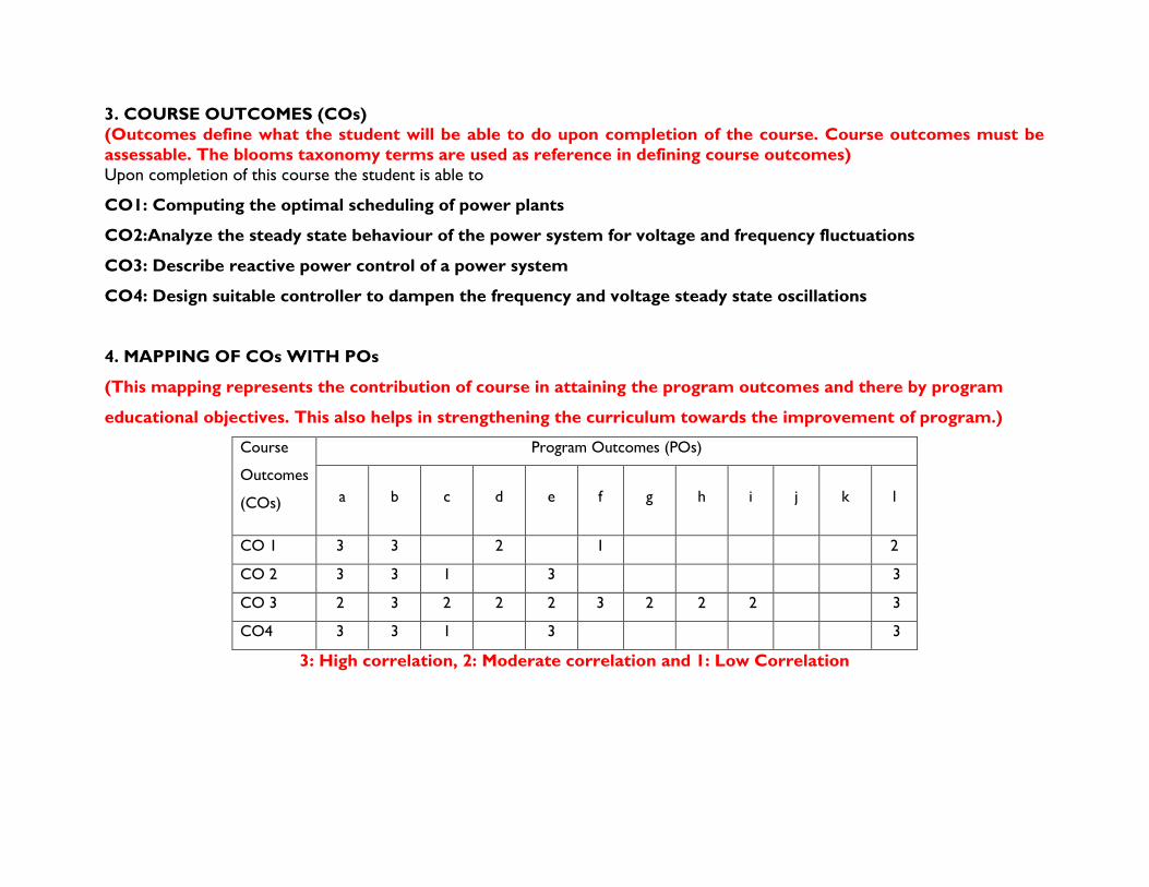
3. COURSE OUTCOMES (COs)
(Outcomes define what the student will be able to do upon completion of the course. Course outcomes must be
assessable. The blooms taxonomy terms are used as reference in defining course outcomes)
Upon completion of this course the student is able to
CO1: Computing the optimal scheduling of power plants
CO2:Analyze the steady state behaviour of the power system for voltage and frequency fluctuations
CO3: Describe reactive power control of a power system
CO4: Design suitable controller to dampen the frequency and voltage steady state oscillations
4. MAPPING OF COs WITH POs
(This mapping represents the contribution of course in attaining the program outcomes and there by program
educational objectives. This also helps in strengthening the curriculum towards the improvement of program.)
Course
Outcomes
(COs)
Program Outcomes (POs)
a b c d e f g h i j k l
CO 1 3 3 2 1 2
CO 2 3 3 1 3 3
CO 3 2 3 2 2 2 3 2 2 2 3
CO4 3 3 1 3 3
3: High correlation, 2: Moderate correlation and 1: Low Correlation

5. LEARNING RESOURCES
(i) TEXT BOOKS
T1. Electric Energy systems Theory – by O.I.Elgerd, Tata Mc Graw-hill Publishing Comapany Ltd., Second edition.
T2. Power system analyaia and Stability by S.S. Vadhera
T3. Power system Operation and control by P.S.R Murthy
T4. Modern Power System Analysis – by I.J.Nagrath & D.P.Kothari Tata M Graw – Hill Publishing Company Ltd, 2nd edition.
(ii) REFERENCES (Publications/ Open Learning Resources)
T1. Power System Analysis and Design by J.Duncan Glover and M.S.Sarma., THOMPSON, 3rd Edition.
T2. Electric Power systems – by B.M.Weedy, B.J.Cary 4th Edition , Wiley.
T3. Economic Operation of Power systems – by L.K.Kirchmayer, Wiley Eastern Ltd.
T4. Power System Analysis by N.V.Ramana and N.Yadaiah, Pearson Education.
(Course delivery including latest trends brings good insight of the course in students and also inculcates the habit of
self learning among the students.
Publications referred can be given unit wise or at course level.)
(a) Publications
Unit I
1. "Digital computer directs automatic dispatching control system," in Electrical Engineering, vol. 80, no. 10, pp. 795-796, Oct.
1961
2. H. Isoda and Y. Sato, "On-Line Load Dispatching Control with Security Constraints at the Tohoku Electric Power
Company," in IEEE Power Engineering Review, vol. PER-5, no. 6, pp. 34-35, June 1985.
3. R. Bhatnagar and S. Rahman, "Dispatch of Direct Load Control for Fuel Cost Minimization," in IEEE Power Engineering
Review, vol. PER-6, no. 11, pp. 34-34, Nov. 1986
4. R. H. Kerr and L. K. Kirchmayer, "Theory of Economic Operation of Interconnected Areas," in Transactions of the American
Institute of Electrical Engineers. Part III: Power Apparatus and Systems, vol. 78, no. 3, pp. 647-653, April 1959.
Unit-II
1. "Digital computer directs automatic dispatching control system," in Electrical Engineering, vol. 80, no. 10, pp. 795-796, Oct.
1961
2. H. Isoda and Y. Sato, "On-Line Load Dispatching Control with Security Constraints at the Tohoku Electric Power
Company," in IEEE Power Engineering Review, vol. PER-5, no. 6, pp. 34-35, June 1985.
3. R. Bhatnagar and S. Rahman, "Dispatch of Direct Load Control for Fuel Cost Minimization," in IEEE Power Engineering
Review, vol. PER-6, no. 11, pp. 34-34, Nov. 1986
4. R. H. Kerr and L. K. Kirchmayer, "Theory of Economic Operation of Interconnected Areas," in Transactions of the American
Institute of Electrical Engineers. Part III: Power Apparatus and Systems, vol. 78, no. 3, pp. 647-653, April 1959.
Unit-III
1. L. B. Wales, "Performance characteristics of speed governors," in Electrical Engineering, vol. 68, no. 3, pp. 198-198, March
1949
2. "Recommended Specifications for Speed-Governing of Steam Turbines Intended to Drive Electric Generators Rated 500
Kw and Larger Aiee-Asme Committee Report," in Transactions of the American Institute of Electrical Engineers. Part III: Power
Apparatus and Systems, vol. 76, no. 3, pp. 1404-1411, April 1957
3. Y. Y. Hsu, S. W. Shyue and C. C. Su, "Low Frequency Oscillations in Longitudinal Power Systems: Experience with Dynamic
Stability of Taiwan Power System," in IEEE Transactions on Power Systems, vol. 2, no. 1, pp. 92-98, Feb. 1987.
4. En Lu, Ning Wang, Zhijun Qin, Haoming Liu and Yunhe Hou, "Black-start strategy for power grids including fast cut thermal
power units," 2013 IEEE Power & Energy Society General Meeting, Vancouver, BC, 2013, pp. 1-5
Unit-IV
1. M. P. Musau, T. L. Chepkania, A. N. Odero and C. W. Wekesa, "Effects of renewable energy on frequency stability: A
proposed case study of the Kenyan grid," 2017 IEEE PES PowerAfrica, Accra, 2017, pp. 12-15.
2. C. A. Ruiz, N. J. Orrego and J. F. Gutierrez, "The Colombian 2007 black out," 2008 IEEE/PES Transmission and Distribution
Conference and Exposition: Latin America, Bogota, 2008, pp. 1-5.
3. M. A. Abdel-Halim, G. S. Christensen and D. H. Kelly, "Optimum load frequency control of multi-area interconnected
power systems," in Canadian Electrical Engineering Journal, vol. 10, no. 1, pp. 32-39, Jan. 1985.
4. H. M. Dimond and G. S. Lunge, "Interconnected system load-frequency control," in Electrical Engineering, vol. 68, no. 2, pp.
162-162, Feb. 1949.
Unit-V
1. J. Zaborszky, G. Huang and K. W. Lu, "A Textured Model for Computationally Efficient Reactive Power Control and
Management," in IEEE Power Engineering Review, vol. PER-5, no. 7, pp. 35-36, July 1985
2. M. M. A. Salama, A. Y. Chikhani and R. Hackam, "Control of Reactive Power in Distribution Systems with an End-Load and
Fixed Load Condition," in IEEE Power Engineering Review, vol. PER-5, no. 10, pp. 39-39, Oct. 1985
3. En Lu, Ning Wang, Zhijun Qin, Haoming Liu and Yunhe Hou, "Black-start strategy for power grids including fast cut thermal
power units," 2013 IEEE Power & Energy Society General Meeting, Vancouver, BC, 2013, pp. 1-5
(b) Open Learning Resources for self learning
L1. http://nptel.ac.in/courses/108101040/
L2. https://ocw.mit.edu/courses/engineering-systems-division/esd-934-engineering-economics-and-regulation-of-the-electric-power-
sector-spring-2010/
L3. https://www.coursera.org/learn/electricity
L4:http://www.cdeep.iitb.ac.in/webpage_data/nptel/Electrical%20Engineering/Power%20System%20Operation%20and%20Control/d
ownloads/POWER%20SYSTEM%20OPERATION.pdf
L5. www.srldc.org
(iii) JOURNALS
J1. IEEE Journal on Power Delivery.
J2. Electrical Power components and Systems.
J3.Electricsl Power systems research.
J4. IEEE journal on Power Sytems.
6. DELIVERY METHODOLOGIES
(Depending on the suitability to the delivery of concept, one or more among the following delivery methodologies
are adopted to engage the student in learning)
DM1: Chalk and Talk DM5: Open The Box
DM3: Collaborative Learning (Think Pair Share, POGIL, etc.) DM7: Group Project
DM4: Demonstration (Physical / Laboratory / Audio Visuals)
7. PROPOSED FIELD VISITS/ GUEST LECTURE BY INDUSTRY EXPERT
(To be added for the courses as directed by the department.)
Guest Lecture: "New challenges in maintaining Power systems stable" by Mr.SatyaPrasad , Divisional engineer, APTRansco on
14/10/17
(And / Or)
Field Visit: As a part of class, field visit is scheduled to Hydro electric Plant on 21/10/2017.
8. ASSESSMENT
(As per Regulations, AM1 and AM2 are compulsory for assessment. Whereas, any two or more assessment
methodologies can be considered from AM3 to AM9 under assignment towards continuous assessment of the
performance of students.)
AM1: Semester End Examination . AM2: Mid Term Examination
AM3: Home Assignments
AM6: Quizzes
AM7: Course Projects**
* (To be added for the courses as directed by the department. The no. of course projects is left to the liberty of
faculty)
9. WEIGHTAGES FOR PROPOSED ASSESSMENT METHODOLOGIES
(The allotted marks for home assignments, quizzes and etc., except course projects are left to the liberty of
faculty. But for the finalisation of assignment marks, the following weightages can be considered.)
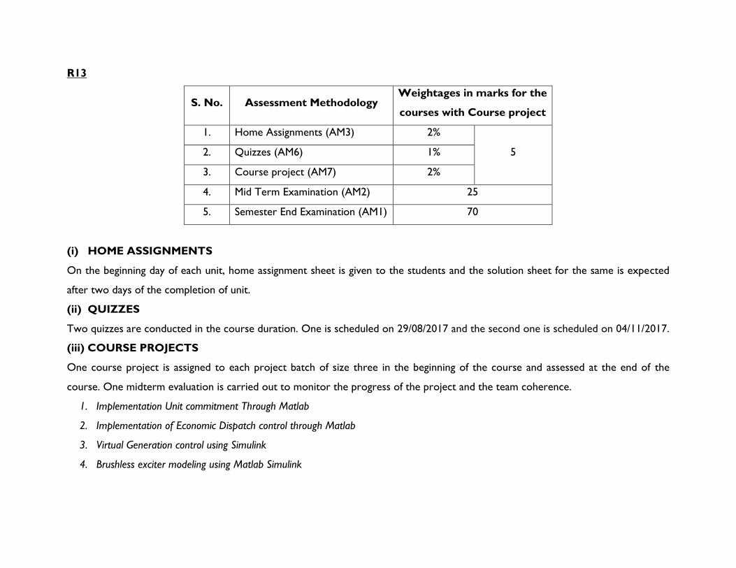
R13
S. No. Assessment Methodology Weightages in marks for the
courses with Course project
1. Home Assignments (AM3) 2%
5 2. Quizzes (AM6) 1%
3. Course project (AM7) 2%
4. Mid Term Examination (AM2) 25
5. Semester End Examination (AM1) 70
(i) HOME ASSIGNMENTS
On the beginning day of each unit, home assignment sheet is given to the students and the solution sheet for the same is expected
after two days of the completion of unit.
(ii) QUIZZES
Two quizzes are conducted in the course duration. One is scheduled on 29/08/2017 and the second one is scheduled on 04/11/2017.
(iii) COURSE PROJECTS
One course project is assigned to each project batch of size three in the beginning of the course and assessed at the end of the
course. One midterm evaluation is carried out to monitor the progress of the project and the team coherence.
1. Implementation Unit commitment Through Matlab
2. Implementation of Economic Dispatch control through Matlab
3. Virtual Generation control using Simulink
4. Brushless exciter modeling using Matlab Simulink

10. SIMULATION SOFTWARES (If any)
11. MATLAB
12. Mi Power
13. PS CAD
11. DETAILED COURSE DELIVERY PLAN
(Detailed syllabus mentioning its learning outcomes, teaching plan, tutorial questions and home assignment
questions for each unit can be given. Heads under teaching plan is given below. Model Academic plan can be taken
as reference.)
UNIT -I
Economic Operation of Power Systems : Optimal operation of Generators in Thermal Power Stations, - heat rate Curve – Cost
Curve – Incremental fuel and Production costs, input-output characteristics, Optimum generation allocation with line losses
neglected. Optimum generation allocation including the effect of transmission line losses – Loss Coefficients, General
transmission line loss formula.
LEARNING OUTCOMES
After completion of this unit the student will be able to
After Completion of this unit, student must be able to
1. Know the meaning of control and operation of Power System
2. Define what is Optimum operation of generators
3. Know the IFC
4. Draw input-output characteristics of thermal power station
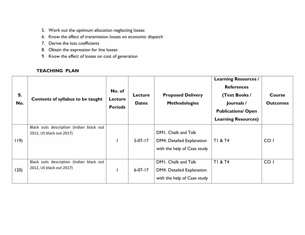
5. Work out the optimum allocation neglecting losses
6. Know the effect of transmission losses on economic dispatch
7. Derive the loss coefficients
8. Obtain the expression for line losses
9. Know the effect of losses on cost of generation
TEACHING PLAN
S.
No. Contents of syllabus to be taught
No. of
Lecture
Periods
Lecture
Dates
Proposed Delivery
Methodologies
Learning Resources /
References
(Text Books /
Journals /
Publications/ Open
Learning Resources)
Course
Outcomes
119)
Black outs description (Indian black out
2012, US black out 2017)
1 5-07-17
DM1. Chalk and Talk
DM4. Detailed Explanation
with the help of Case study
T1 & T4 CO 1
120)
Black outs description (Indian black out
2012, US black out 2017) 1 6-07-17
DM1. Chalk and Talk
DM4. Detailed Explanation
with the help of Case study
T1 & T4 CO 1
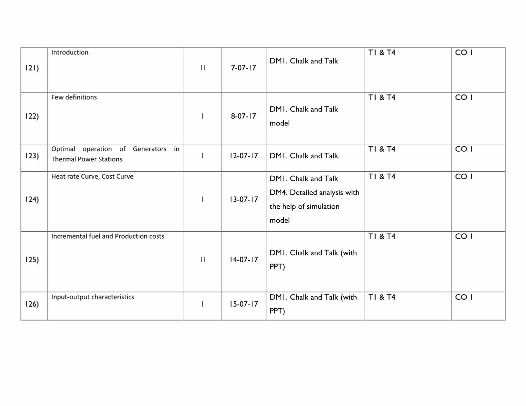
121)
Introduction
1I 7-07-17 DM1. Chalk and Talk
T1 & T4 CO 1
122)
Few definitions
1 8-07-17 DM1. Chalk and Talk
model
T1 & T4 CO 1
123) Optimal operation of Generators in
Thermal Power Stations 1 12-07-17 DM1. Chalk and Talk. T1 & T4 CO 1
124)
Heat rate Curve, Cost Curve
1 13-07-17
DM1. Chalk and Talk
DM4. Detailed analysis with
the help of simulation
model
T1 & T4 CO 1
125)
Incremental fuel and Production costs
1I 14-07-17 DM1. Chalk and Talk (with
PPT)
T1 & T4 CO 1
126) Input-output characteristics
1 15-07-17 DM1. Chalk and Talk (with
PPT)
T1 & T4 CO 1

127)
Optimum generation allocation with line
losses neglected
1 19-07-17
DM1. Chalk and Talk
DM4. Detailed analysis with
the help of case study
T1 & T4 CO 1
128)
Problems
1 20-07-17 DM1. Chalk and Talk
T1 & T4 CO 1
129)
Optimum generation allocation including
the effect of transmission line losses, Loss
Coefficients 1I 21/07/17
DM1. Chalk and Talk
DM4. Detailed analysis with
case tudy
T1 & T4 CO 1
130)
General transmission line loss formula
1 22/07/17 DM1. Chalk and Talk
T1 & T4 CO 1
131) Problems
1 26/07/17 DM1. Chalk and Talk
DM3. Collaborative learning
T1 & T4 CO 1
132) Recent Trends in Power system
control I 27/07/17
DM1. Chalk and Talk
DM3. Collaborative learning
T1 & T4
133) Assignment Questions Discussion
1I 28/07/17 DM1. Chalk and Talk
DM3. Collaborative learning
CO 1
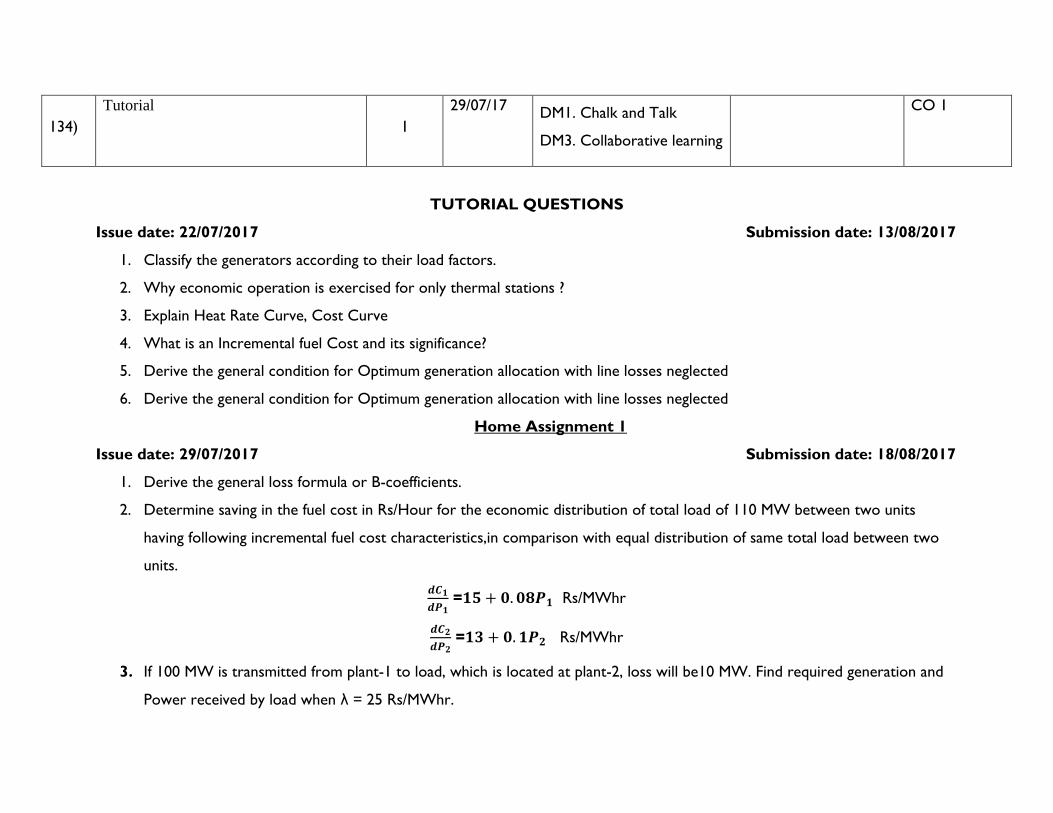
134)
Tutorial
1
29/07/17 DM1. Chalk and Talk
DM3. Collaborative learning
CO 1
TUTORIAL QUESTIONS
Issue date: 22/07/2017 Submission date: 13/08/2017
1. Classify the generators according to their load factors.
2. Why economic operation is exercised for only thermal stations ?
3. Explain Heat Rate Curve, Cost Curve
4. What is an Incremental fuel Cost and its significance?
5. Derive the general condition for Optimum generation allocation with line losses neglected
6. Derive the general condition for Optimum generation allocation with line losses neglected
Home Assignment 1
Issue date: 29/07/2017 Submission date: 18/08/2017
1. Derive the general loss formula or B-coefficients.
2. Determine saving in the fuel cost in Rs/Hour for the economic distribution of total load of 110 MW between two units
having following incremental fuel cost characteristics,in comparison with equal distribution of same total load between two
units.
𝒅𝑪𝟏
𝒅𝑷𝟏 =𝟏𝟓 + 𝟎. 𝟎𝟖𝑷𝟏 Rs/MWhr
𝒅𝑪𝟐
𝒅𝑷𝟐 =𝟏𝟑 + 𝟎. 𝟏𝑷𝟐 Rs/MWhr
3. If 100 MW is transmitted from plant-1 to load, which is located at plant-2, loss will be10 MW. Find required generation and
Power received by load when λ = 25 Rs/MWhr.
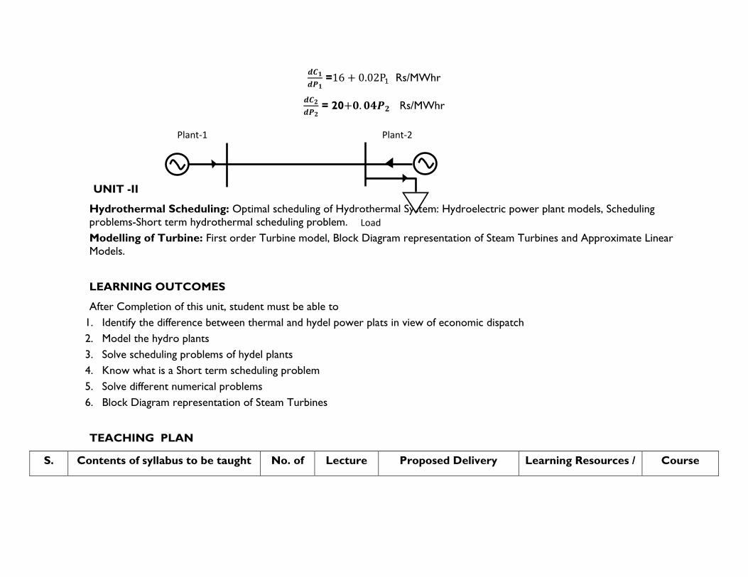
𝒅𝑪𝟏
𝒅𝑷𝟏 =16 + 0.02P1 Rs/MWhr
𝒅𝑪𝟐
𝒅𝑷𝟐 = 20+𝟎. 𝟎𝟒𝑷𝟐 Rs/MWhr
UNIT -II
Hydrothermal Scheduling: Optimal scheduling of Hydrothermal System: Hydroelectric power plant models, Scheduling
problems-Short term hydrothermal scheduling problem.
Modelling of Turbine: First order Turbine model, Block Diagram representation of Steam Turbines and Approximate Linear
Models.
LEARNING OUTCOMES
After Completion of this unit, student must be able to
1. Identify the difference between thermal and hydel power plats in view of economic dispatch
2. Model the hydro plants
3. Solve scheduling problems of hydel plants
4. Know what is a Short term scheduling problem
5. Solve different numerical problems
6. Block Diagram representation of Steam Turbines
TEACHING PLAN
S. Contents of syllabus to be taught No. of Lecture Proposed Delivery Learning Resources / Course
Plant-1 Plant-2
Load
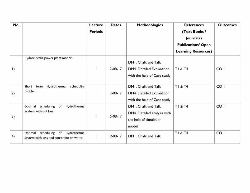
No. Lecture
Periods
Dates Methodologies References
(Text Books /
Journals /
Publications/ Open
Learning Resources)
Outcomes
1)
Hydroelectric power plant models
1 2-08-17
DM1. Chalk and Talk
DM4. Detailed Explanation
with the help of Case study
T1 & T4 CO 1
2)
Short term Hydrothermal scheduling
problem 1 3-08-17
DM1. Chalk and Talk
DM4. Detailed Explanation
with the help of Case study
T1 & T4 CO 1
3)
Optimal scheduling of Hydrothermal
System with out loss
1 5-08-17
DM1. Chalk and Talk
DM4. Detailed analysis with
the help of simulation
model
T1 & T4 CO 1
4) Optimal scheduling of Hydrothermal
System with loss and constraint on water 1 9-08-17 DM1. Chalk and Talk. T1 & T4 CO 1
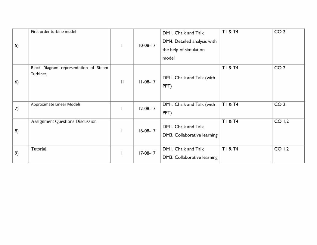
5)
First order turbine model
1 10-08-17
DM1. Chalk and Talk
DM4. Detailed analysis with
the help of simulation
model
T1 & T4 CO 2
6)
Block Diagram representation of Steam
Turbines
1I 11-08-17 DM1. Chalk and Talk (with
PPT)
T1 & T4 CO 2
7) Approximate Linear Models
1 12-08-17 DM1. Chalk and Talk (with
PPT)
T1 & T4 CO 2
8)
Assignment Questions Discussion
1 16-08-17 DM1. Chalk and Talk
DM3. Collaborative learning
T1 & T4 CO 1,2
9) Tutorial
1 17-08-17 DM1. Chalk and Talk
DM3. Collaborative learning
T1 & T4 CO 1,2
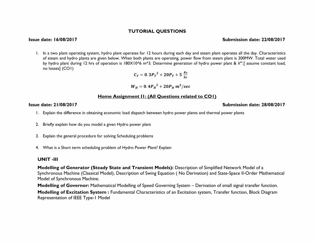
TUTORIAL QUESTIONS
Issue date: 16/08/2017 Submission date: 22/08/2017
1. In a two plant operating system, hydro plant operates for 12 hours during each day and steam plant operates all the day. Characteristics
of steam and hydro plants are given below. When both plants are operating, power flow from steam plant is 300MW. Total water used
by hydro plant during 12 hrs of operation is 180X10^6 m^3. Determine generation of hydro power plant & λ”.[ assume constant load,
no losses] (CO1)
𝑪𝑻 = 𝟎. 𝟑𝑷𝑻𝟐 + 𝟐𝟎𝑷𝑻 + 𝟓
𝑹𝒔
𝒉𝒓
𝑾𝑯 = 𝟎. 𝟒𝑷𝑯𝟐 + 𝟐𝟎𝑷𝑯 𝒎𝟑/𝒔𝒆𝒄
Home Assignment I1: (All Questions related to CO1)
Issue date: 21/08/2017 Submission date: 28/08/2017
1. Explain the difference in obtaining economic load dispatch between hydro power plants and thermal power plants
2. Briefly explain how do you model a given Hydro power plant
3. Explain the general procedure for solving Scheduling problems
4. What is a Short term scheduling problem of Hydro Power Plant? Explain
UNIT -III
Modelling of Generator (Steady State and Transient Models): Description of Simplified Network Model of a
Synchronous Machine (Classical Model), Description of Swing Equation ( No Derivation) and State-Space II-Order Mathematical
Model of Synchronous Machine.
Modelling of Governor: Mathematical Modelling of Speed Governing System – Derivation of small signal transfer function.
Modelling of Excitation System : Fundamental Characteristics of an Excitation system, Transfer function, Block Diagram
Representation of IEEE Type-1 Model
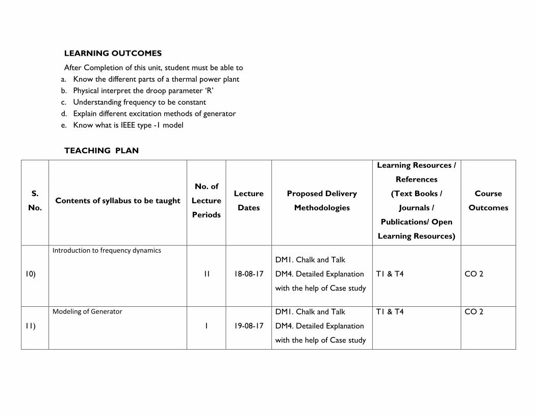
LEARNING OUTCOMES
After Completion of this unit, student must be able to
a. Know the different parts of a thermal power plant
b. Physical interpret the droop parameter ‘R’
c. Understanding frequency to be constant
d. Explain different excitation methods of generator
e. Know what is IEEE type -1 model
TEACHING PLAN
S.
No. Contents of syllabus to be taught
No. of
Lecture
Periods
Lecture
Dates
Proposed Delivery
Methodologies
Learning Resources /
References
(Text Books /
Journals /
Publications/ Open
Learning Resources)
Course
Outcomes
10)
Introduction to frequency dynamics
1I 18-08-17
DM1. Chalk and Talk
DM4. Detailed Explanation
with the help of Case study
T1 & T4 CO 2
11)
Modeling of Generator
1 19-08-17
DM1. Chalk and Talk
DM4. Detailed Explanation
with the help of Case study
T1 & T4 CO 2
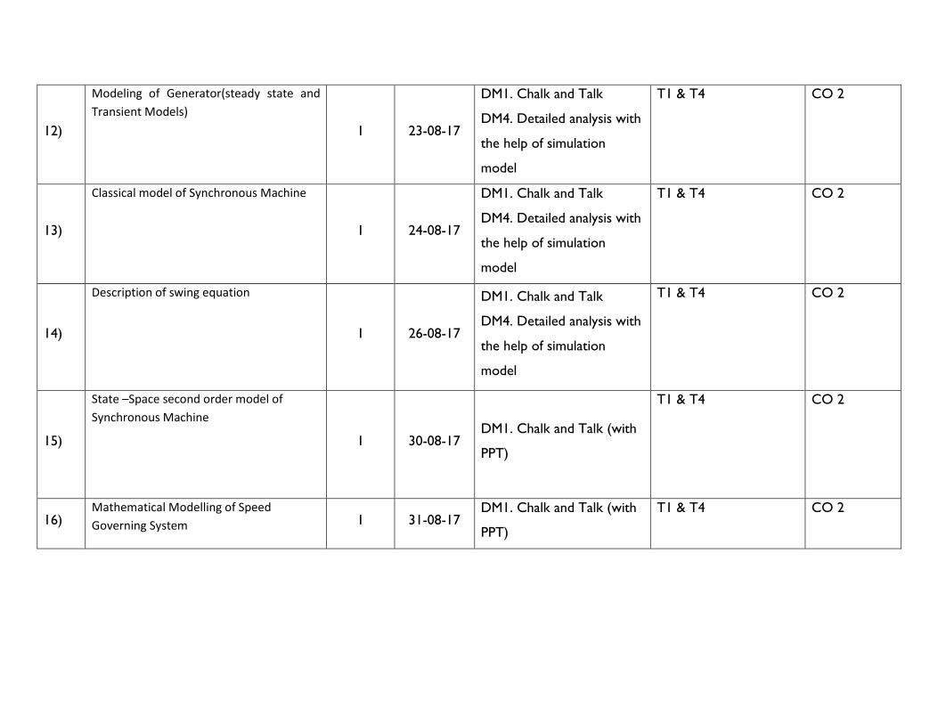
12)
Modeling of Generator(steady state and
Transient Models)
1 23-08-17
DM1. Chalk and Talk
DM4. Detailed analysis with
the help of simulation
model
T1 & T4 CO 2
13)
Classical model of Synchronous Machine
1 24-08-17
DM1. Chalk and Talk
DM4. Detailed analysis with
the help of simulation
model
T1 & T4 CO 2
14)
Description of swing equation
1 26-08-17
DM1. Chalk and Talk
DM4. Detailed analysis with
the help of simulation
model
T1 & T4 CO 2
15)
State –Space second order model of
Synchronous Machine
1 30-08-17 DM1. Chalk and Talk (with
PPT)
T1 & T4 CO 2
16) Mathematical Modelling of Speed
Governing System 1 31-08-17 DM1. Chalk and Talk (with
PPT)
T1 & T4 CO 2

17)
Deviation of small signal transfer function,
Modeling of Excitation System
1I 1-09-17
DM1. Chalk and Talk
DM4. Detailed analysis with
the help of case study
T1 & T4 CO 2
18)
Fundamental characteristics of an
Excitation Syastem,Transfer function
1 2-09-17 DM1. Chalk and Talk
T1 & T4 CO 2
19)
Block Diagram Represantation of IEEE
Type-1 Model
1 13-9-17 DM1. Chalk and Talk (with
PPT)
T1 & T4 CO 2
20)
Assignment Questions Discussion
1 14-9-17 DM1. Chalk and Talk
DM3: Collaborative learning
T1 & T4 CO 2
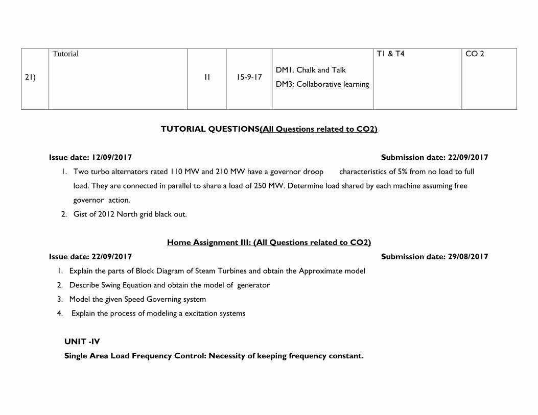
21)
Tutorial
1I 15-9-17 DM1. Chalk and Talk
DM3: Collaborative learning
T1 & T4 CO 2
TUTORIAL QUESTIONS(All Questions related to CO2)
Issue date: 12/09/2017 Submission date: 22/09/2017
1. Two turbo alternators rated 110 MW and 210 MW have a governor droop characteristics of 5% from no load to full
load. They are connected in parallel to share a load of 250 MW. Determine load shared by each machine assuming free
governor action.
2. Gist of 2012 North grid black out.
Home Assignment III: (All Questions related to CO2)
Issue date: 22/09/2017 Submission date: 29/08/2017
1. Explain the parts of Block Diagram of Steam Turbines and obtain the Approximate model
2. Describe Swing Equation and obtain the model of generator
3. Model the given Speed Governing system
4. Explain the process of modeling a excitation systems
UNIT -IV
Single Area Load Frequency Control: Necessity of keeping frequency constant.
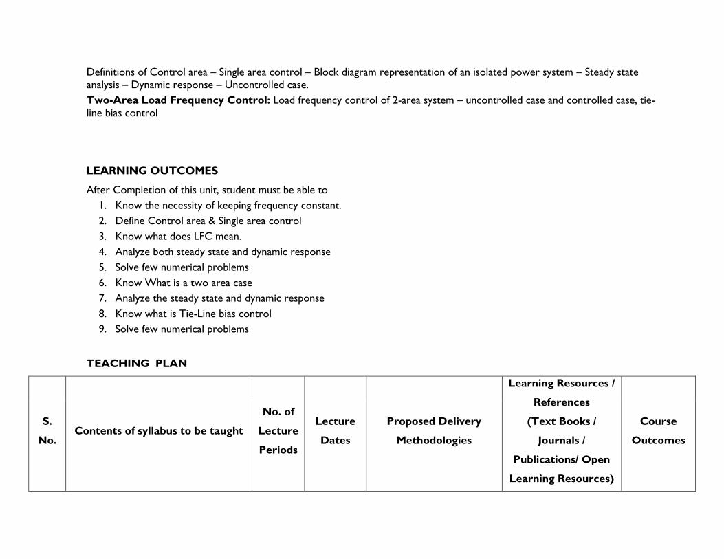
Definitions of Control area – Single area control – Block diagram representation of an isolated power system – Steady state
analysis – Dynamic response – Uncontrolled case.
Two-Area Load Frequency Control: Load frequency control of 2-area system – uncontrolled case and controlled case, tie-
line bias control
LEARNING OUTCOMES
After Completion of this unit, student must be able to
1. Know the necessity of keeping frequency constant.
2. Define Control area & Single area control
3. Know what does LFC mean.
4. Analyze both steady state and dynamic response
5. Solve few numerical problems
6. Know What is a two area case
7. Analyze the steady state and dynamic response
8. Know what is Tie-Line bias control
9. Solve few numerical problems
TEACHING PLAN
S.
No. Contents of syllabus to be taught
No. of
Lecture
Periods
Lecture
Dates
Proposed Delivery
Methodologies
Learning Resources /
References
(Text Books /
Journals /
Publications/ Open
Learning Resources)
Course
Outcomes
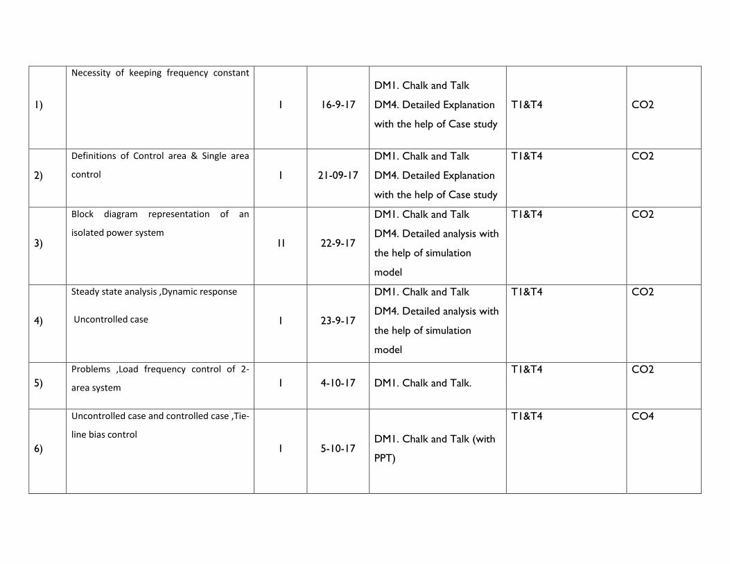
1)
Necessity of keeping frequency constant
1 16-9-17
DM1. Chalk and Talk
DM4. Detailed Explanation
with the help of Case study
T1&T4 CO2
2)
Definitions of Control area & Single area
control 1 21-09-17
DM1. Chalk and Talk
DM4. Detailed Explanation
with the help of Case study
T1&T4 CO2
3)
Block diagram representation of an
isolated power system 1I 22-9-17
DM1. Chalk and Talk
DM4. Detailed analysis with
the help of simulation
model
T1&T4 CO2
4)
Steady state analysis ,Dynamic response
Uncontrolled case 1 23-9-17
DM1. Chalk and Talk
DM4. Detailed analysis with
the help of simulation
model
T1&T4 CO2
5)
Problems ,Load frequency control of 2-
area system 1 4-10-17 DM1. Chalk and Talk.
T1&T4 CO2
6)
Uncontrolled case and controlled case ,Tie-
line bias control
I 5-10-17 DM1. Chalk and Talk (with
PPT)
T1&T4 CO4
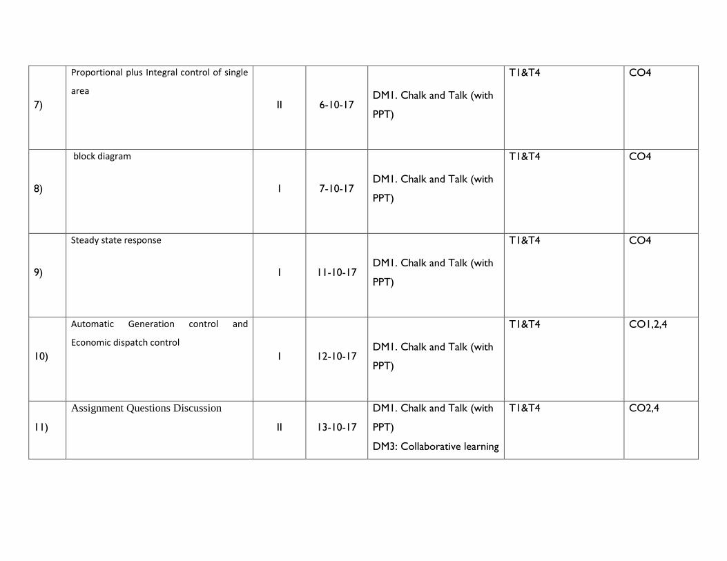
7)
Proportional plus Integral control of single
area
II 6-10-17 DM1. Chalk and Talk (with
PPT)
T1&T4 CO4
8)
block diagram
I 7-10-17 DM1. Chalk and Talk (with
PPT)
T1&T4 CO4
9)
Steady state response
I 11-10-17 DM1. Chalk and Talk (with
PPT)
T1&T4 CO4
10)
Automatic Generation control and
Economic dispatch control
I 12-10-17 DM1. Chalk and Talk (with
PPT)
T1&T4 CO1,2,4
11)
Assignment Questions Discussion
II 13-10-17
DM1. Chalk and Talk (with
PPT)
DM3: Collaborative learning
T1&T4 CO2,4
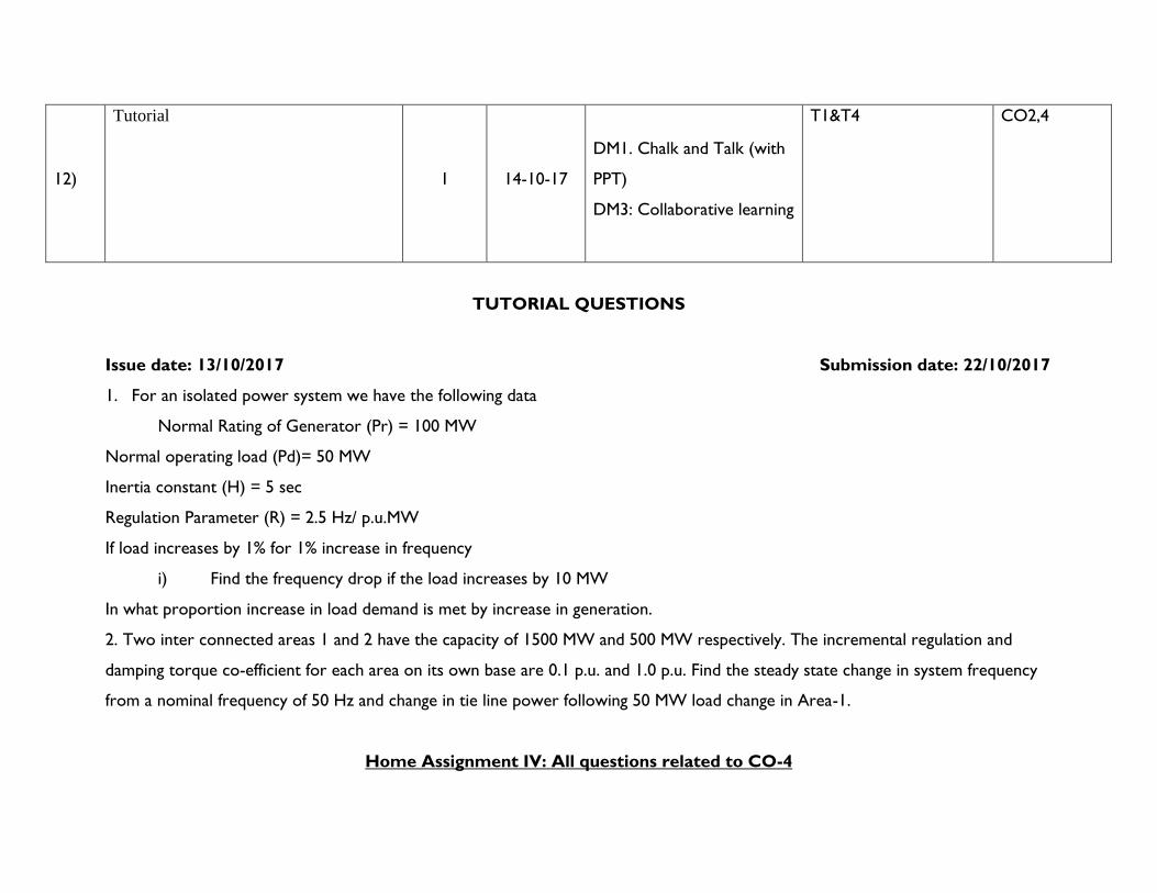
12)
Tutorial
I 14-10-17
DM1. Chalk and Talk (with
PPT)
DM3: Collaborative learning
T1&T4 CO2,4
TUTORIAL QUESTIONS
Issue date: 13/10/2017 Submission date: 22/10/2017
1. For an isolated power system we have the following data
Normal Rating of Generator (Pr) = 100 MW
Normal operating load (Pd)= 50 MW
Inertia constant (H) = 5 sec
Regulation Parameter (R) = 2.5 Hz/ p.u.MW
If load increases by 1% for 1% increase in frequency
i) Find the frequency drop if the load increases by 10 MW
In what proportion increase in load demand is met by increase in generation.
2. Two inter connected areas 1 and 2 have the capacity of 1500 MW and 500 MW respectively. The incremental regulation and
damping torque co-efficient for each area on its own base are 0.1 p.u. and 1.0 p.u. Find the steady state change in system frequency
from a nominal frequency of 50 Hz and change in tie line power following 50 MW load change in Area-1.
Home Assignment IV: All questions related to CO-4
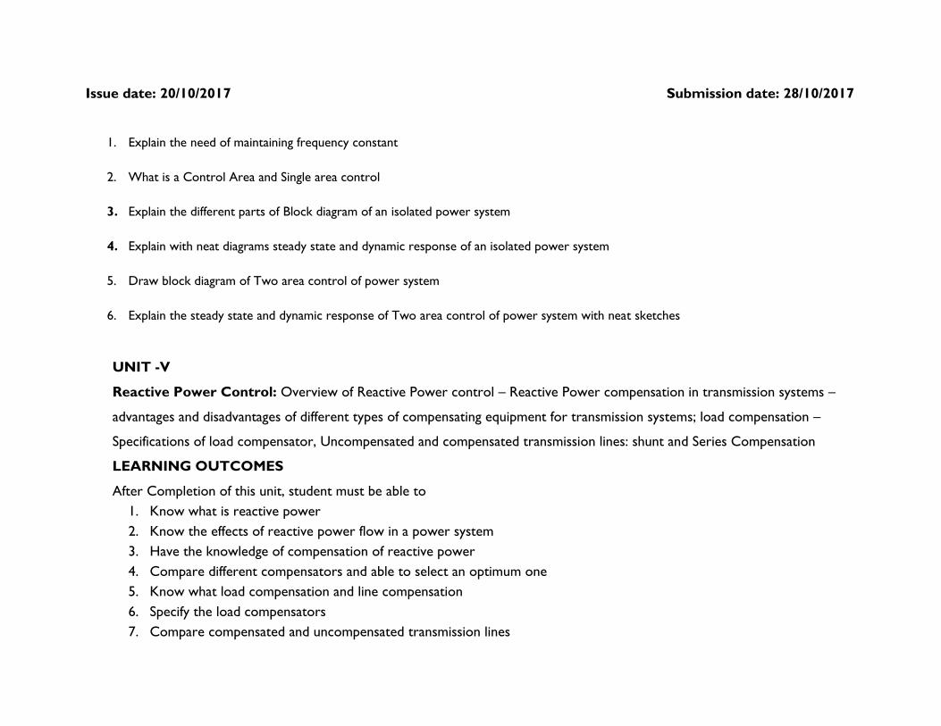
Issue date: 20/10/2017 Submission date: 28/10/2017
1. Explain the need of maintaining frequency constant
2. What is a Control Area and Single area control
3. Explain the different parts of Block diagram of an isolated power system
4. Explain with neat diagrams steady state and dynamic response of an isolated power system
5. Draw block diagram of Two area control of power system
6. Explain the steady state and dynamic response of Two area control of power system with neat sketches
UNIT -V
Reactive Power Control: Overview of Reactive Power control – Reactive Power compensation in transmission systems –
advantages and disadvantages of different types of compensating equipment for transmission systems; load compensation –
Specifications of load compensator, Uncompensated and compensated transmission lines: shunt and Series Compensation
LEARNING OUTCOMES
After Completion of this unit, student must be able to
1. Know what is reactive power
2. Know the effects of reactive power flow in a power system
3. Have the knowledge of compensation of reactive power
4. Compare different compensators and able to select an optimum one
5. Know what load compensation and line compensation
6. Specify the load compensators
7. Compare compensated and uncompensated transmission lines
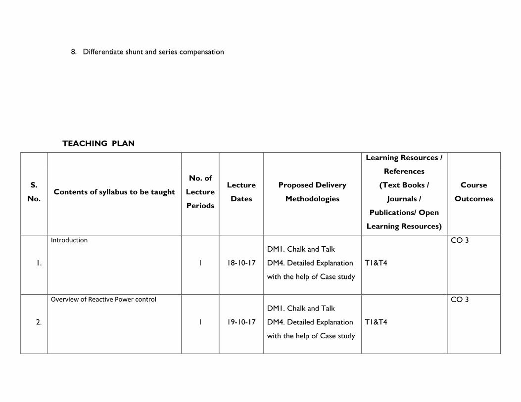
8. Differentiate shunt and series compensation
TEACHING PLAN
S.
No. Contents of syllabus to be taught
No. of
Lecture
Periods
Lecture
Dates
Proposed Delivery
Methodologies
Learning Resources /
References
(Text Books /
Journals /
Publications/ Open
Learning Resources)
Course
Outcomes
1.
Introduction
I 18-10-17
DM1. Chalk and Talk
DM4. Detailed Explanation
with the help of Case study
T1&T4
CO 3
2.
Overview of Reactive Power control
1 19-10-17
DM1. Chalk and Talk
DM4. Detailed Explanation
with the help of Case study
T1&T4
CO 3

3.
Reactive Power compensation in Tr. Lines
1I 20-10-17
DM1. Chalk and Talk
DM4. Detailed Explanation
with the help of Case study
T1&T4 CO 3
4.
Advantages of different types of
compensating equipment for transmission
systems
I 21-10-17
DM1. Chalk and Talk
DM4. Detailed Explanation
with the help of Case study
T1&T4 CO 3
5.
Disadvantages of different types of
compensating equipment for transmission
systems
1 25-10-17
DM1. Chalk and Talk
DM4. Detailed analysis with
the help of case study
T1&T4 CO 3
6.
Load Compensation
1 26-10-17
DM1. Chalk and Talk
DM4. Detailed analysis with
the help of case study
T1&T4 CO 3
7. Specifications of load compensator 1I 27-10-17 DM1. Chalk and Talk. T1&T4 CO 3
8.
Uncompensated Transmission lines
1 28-10-17
DM1. Chalk and Talk
DM4. Detailed analysis with
the help of case study
T1&T4 CO 3
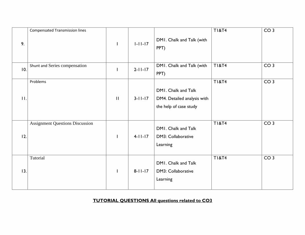
9.
Compensated Transmission lines
1 1-11-17 DM1. Chalk and Talk (with
PPT)
T1&T4 CO 3
10. Shunt and Series compensation
1 2-11-17 DM1. Chalk and Talk (with
PPT)
T1&T4 CO 3
11.
Problems
1I 3-11-17
DM1. Chalk and Talk
DM4. Detailed analysis with
the help of case study
T1&T4 CO 3
12.
Assignment Questions Discussion
1 4-11-17
DM1. Chalk and Talk
DM3: Collaborative
Learning
T1&T4 CO 3
13.
Tutorial
1 8-11-17
DM1. Chalk and Talk
DM3: Collaborative
Learning
T1&T4 CO 3
TUTORIAL QUESTIONS All questions related to CO3
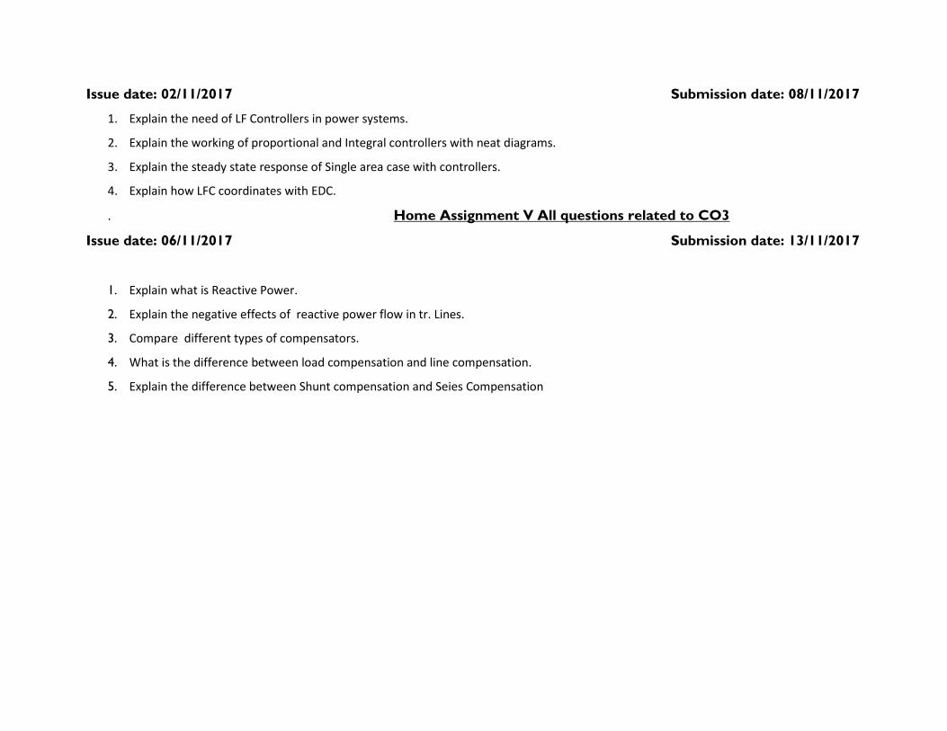
Issue date: 02/11/2017 Submission date: 08/11/2017
1. Explain the need of LF Controllers in power systems.
2. Explain the working of proportional and Integral controllers with neat diagrams.
3. Explain the steady state response of Single area case with controllers.
4. Explain how LFC coordinates with EDC.
. Home Assignment V All questions related to CO3
Issue date: 06/11/2017 Submission date: 13/11/2017
1. Explain what is Reactive Power.
2. Explain the negative effects of reactive power flow in tr. Lines.
3. Compare different types of compensators.
4. What is the difference between load compensation and line compensation.
5. Explain the difference between Shunt compensation and Seies Compensation

12. MODEL QUESTION PAPER
VNR VIGNANA JYOTHI INSTITUTE OF ENGINEERING & TECHNOLOGY
(AN AUTONOMOUS INSTITUTE)
IV B.TECH. I SEMESTER REGULAR EXAMINATION-2017
SUBJECT: POWER SYSTEM OPERATION AND CONTROL
(EEE)
Time: 3 Hours Max. Marks: 70
------------------------------------------------------------------------------------------------------------------------------------------------------------------
Answer all the questions. 5X1=5
1. What is Heat Rate Curve.
2. What is an Incremental fuel Cost.
3. What is the difference between load compensation.
4. What is the advantage of interconnection of areas.
5. Why economic operation is exercised for only thermal stations.
Answer all the questions. 5X2=10
Subject Code
13EEE016
R13
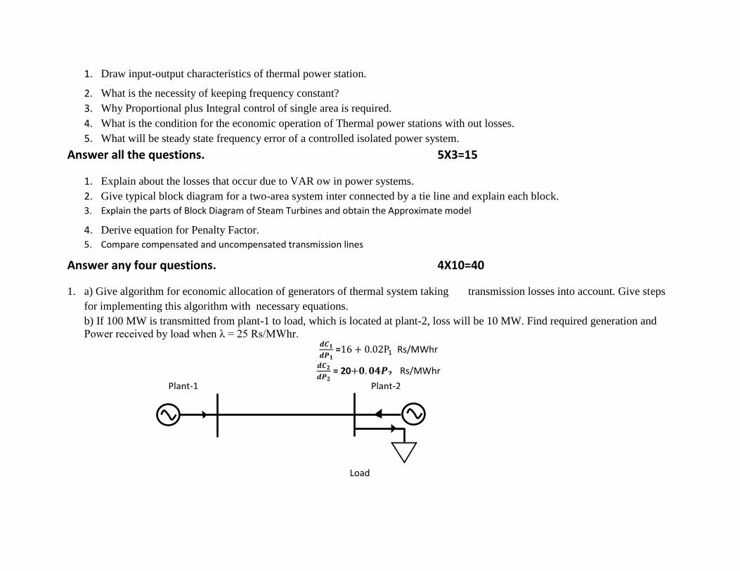
1. Draw input-output characteristics of thermal power station.
2. What is the necessity of keeping frequency constant?
3. Why Proportional plus Integral control of single area is required.
4. What is the condition for the economic operation of Thermal power stations with out losses.
5. What will be steady state frequency error of a controlled isolated power system.
Answer all the questions. 5X3=15
1. Explain about the losses that occur due to VAR ow in power systems.
2. Give typical block diagram for a two-area system inter connected by a tie line and explain each block.
3. Explain the parts of Block Diagram of Steam Turbines and obtain the Approximate model
4. Derive equation for Penalty Factor.
5. Compare compensated and uncompensated transmission lines
Answer any four questions. 4X10=40
1. a) Give algorithm for economic allocation of generators of thermal system taking transmission losses into account. Give steps
for implementing this algorithm with necessary equations.
b) If 100 MW is transmitted from plant-1 to load, which is located at plant-2, loss will be 10 MW. Find required generation and
Power received by load when λ = 25 Rs/MWhr. 𝒅𝑪𝟏
𝒅𝑷𝟏 =16 + 0.02P1 Rs/MWhr
𝒅𝑪𝟐
𝒅𝑷𝟐 = 20+𝟎. 𝟎𝟒𝑷𝟐 Rs/MWhr
Plant-1 Plant-2
Load
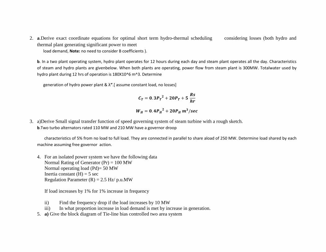
2. a.Derive exact coordinate equations for optimal short term hydro-thermal scheduling considering losses (both hydro and
thermal plant generating significant power to meet
load demand, Note: no need to consider B coefficients ).
b. In a two plant operating system, hydro plant operates for 12 hours during each day and steam plant operates all the day. Characteristics
of steam and hydro plants are givenbelow. When both plants are operating, power flow from steam plant is 300MW. Totalwater used by
hydro plant during 12 hrs of operation is 180X10^6 m^3. Determine
generation of hydro power plant & λ”.[ assume constant load, no losses]
𝑪𝑻 = 𝟎. 𝟑𝑷𝑻𝟐 + 𝟐𝟎𝑷𝑻 + 𝟓
𝑹𝒔
𝒉𝒓
𝑾𝑯 = 𝟎. 𝟒𝑷𝑯𝟐 + 𝟐𝟎𝑷𝑯 𝒎𝟑/𝒔𝒆𝒄
3. a)Derive Small signal transfer function of speed governing system of steam turbine with a rough sketch.
b.Two turbo alternators rated 110 MW and 210 MW have a governor droop
characteristics of 5% from no load to full load. They are connected in parallel to share aload of 250 MW. Determine load shared by each
machine assuming free governor action.
4. For an isolated power system we have the following data
Normal Rating of Generator (Pr) = 100 MW
Normal operating load (Pd)= 50 MW
Inertia constant (H) = 5 sec
Regulation Parameter (R) = 2.5 Hz/ p.u.MW
If load increases by 1% for 1% increase in frequency
ii) Find the frequency drop if the load increases by 10 MW
iii) In what proportion increase in load demand is met by increase in generation.
5. a) Give the block diagram of Tie-line bias controlled two area system
b) Derive expression for Tie line power for an uncontrolled two area system.
6. a)How the following devices generate/absorb reactive power.
i) Synchronous machine ii)Over head lines iii)Shunt reactor
b) Two inter connected areas 1 and 2 have the capacity of 1500 MW and 500 MW respectively. The incremental regulation and
damping torque co-efficient for each area on its own base are 0.1 p.u. and 1.0 p.u. Find the steady state change in system
frequency from a nominal frequency of 50 Hz and change in tie line power following 50 MW load change in Area-1.