Embed Size (px)
Citation preview
AC 2008-2725: DESIGN OF EXPERIMENTS APPROACH TO VERIFICATIONAND UNCERTAINTY ESTIMATION OF SIMULATIONS BASED ON FINITEELEMENT METHOD
Jeffrey Fong, National Institute of Standards and TechnologyJeffrey T. Fong was educated at the University of Hong Kong (B.Sc., Engineering, First ClassHonors, 1955), Columbia University (M.S., Engineering Mechanics, 1961), and StanfordUniversity (Ph.D., Applied Mechanics and Mathematics, 1966). From 1955 to 1963, he worked asan engineer in powerplant design and construction at Ebasco Services, Inc. in New York City,and earned a professional engineer's license to practice in the State of New York (P.E., 1962) andthe British Commonwealth (A.M.I.C.E., London, U.K., 1968).
Since 1966, Dr. Fong has been a research engineer with the title of Physicist at the Mathematicaland Computational Sciences Division of the National Institute of Standards and Technology(NIST) in Gaithersburg, Maryland. During his long association with NIST, he has published morethan 80 technical papers and reports, and edited numerous conference proceedings in the areas offatigue and fracture mechanics, nondestructive testing, mathematical and statistical modeling ofinelastic behavior of materials, and engineering safety and failure analysis. In Jan. 2006, Dr. Fongwas appointed Adjunct Visiting Research Professor of Structures and Statistics of the Departmentof Mechanical Engineering and Mechanics, Drexel University, Philadelphia, Pennsylvania, andwas invited to teach graduate-level courses entitled "Finite Element Method with UncertaintyAnalysis," and "Failure Analysis and Engineering Safety."
Elected Fellow of the American Society for Testing and Materials (ASTM) in 1982, Fellow of theAmerican Society of Mechanical Engineers (ASME) in 1984, and an ASME NationalDistinguished Lecturer from 1988 to 1992, Dr. Fong received in 1993 one of ASME's highestawards, the Pressure Vessel and Piping Medal.
James Filliben, National Institute of Standards and TechnologyJames J. Filliben is currently Leader of the Statistical Modeling and Analysis Group in theStatistical Engineering Division of the Information Technology Laboratory at the NationalInstitute of Standards and Technology (NIST), Gaithersburg, Maryland.
He earned his BA (1965) in Mathematics from LaSalle College, and PhD (1969) in Statisticsfrom Princeton University. He joined the technical staff of NIST in 1969, and has more than 50papers in refereed journals and 200 talks and short courses to his credit. In 2003, he became aFellow of the American Statistical Association.
Alan Heckert, National Institute of Standards and TechnologyAlan Heckert earned his B.S. degree in mathematics at the Frostburg State University in 1978,and his M.S. in mathematics/statistics at the Clemson University in 1980. He worked at theCensus Bureau from 1981 to 1985, and has been a Computer Specialist in the StatisticalEngineering Division of the National Institute of Standards and Technology, Gaithersburg,Maryland, since 1985.
Alan Heckert's technical areas of interest are statistical graphics and statistical computing. He is amember of the American Statistical Association and was honored by the U.S. Department ofCommerce (DoC) with the award of a DoC Silver Medal in 2003.
Roland deWit, National Institute of Standards and TechnologyRoland deWit was educated at the Ohio University, Athens, Ohio (B.S., Liberal Arts with majorin Mathematics, 1953), and University of Illinois, Urbana, Illinois (Ph.D., Physics, 1959). Hisprofessional experience has been with the Physics Department, University of Illinois (1959,
© American Society for Engineering Education, 2008

Research Associate), Department of Mineral Technology, University of California, Berkeley, CA(1959-60, Assistant Research Physicist), and the Metallurgy Division of the Materials Scienceand Engineering Laboratory, NIST, Gaithersburg, MD (1960-1998, Physicist (Solid State)). Since1998, he has been a Guest Researcher at NIST and a Consultant based in Potomac, Maryland.
Dr. deWit has published more than 50 technical papers in four major areas: Dislocation Theory(contributed to the development of a continuum theory of dislocations and disclinations); FractureMechanics (participated in the testing and analysis of the dynamic fracture of pressure vesselsteels and the tearing fracture of aluminum sheets with multi-state damage); MechanicalProperties (contributed to the theory of overall elastic properties of polycrystals); and FiniteElement Analysis (developed simulation models for large plastic deformations). He was co-editorof the conference proceedings "Fundamental Aspects of Dislocation Theory" and the "FourthInternational Congress for Stereology," and the English translation of the Russian book"Mechanics of Brittle Fracture" by A. Cherepanov. A number of Dr. deWit's papers have alsobeen translated into Russian and published under the title "Continuum Theory of Disclinations."
© American Society for Engineering Education, 2008
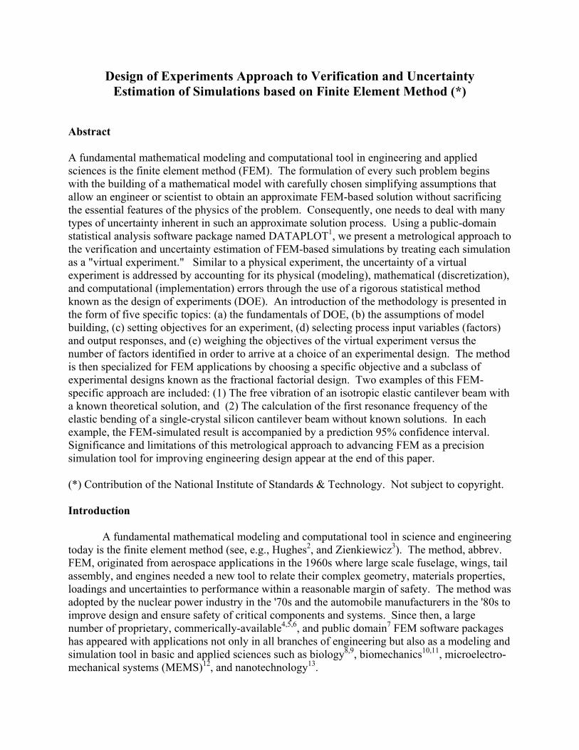
Design of Experiments Approach to Verification and Uncertainty
Estimation of Simulations based on Finite Element Method (*)
Abstract
A fundamental mathematical modeling and computational tool in engineering and applied
sciences is the finite element method (FEM). The formulation of every such problem begins
with the building of a mathematical model with carefully chosen simplifying assumptions that
allow an engineer or scientist to obtain an approximate FEM-based solution without sacrificing
the essential features of the physics of the problem. Consequently, one needs to deal with many
types of uncertainty inherent in such an approximate solution process. Using a public-domain
statistical analysis software package named DATAPLOT1, we present a metrological approach to
the verification and uncertainty estimation of FEM-based simulations by treating each simulation
as a "virtual experiment." Similar to a physical experiment, the uncertainty of a virtual
experiment is addressed by accounting for its physical (modeling), mathematical (discretization),
and computational (implementation) errors through the use of a rigorous statistical method
known as the design of experiments (DOE). An introduction of the methodology is presented in
the form of five specific topics: (a) the fundamentals of DOE, (b) the assumptions of model
building, (c) setting objectives for an experiment, (d) selecting process input variables (factors)
and output responses, and (e) weighing the objectives of the virtual experiment versus the
number of factors identified in order to arrive at a choice of an experimental design. The method
is then specialized for FEM applications by choosing a specific objective and a subclass of
experimental designs known as the fractional factorial design. Two examples of this FEM-
specific approach are included: (1) The free vibration of an isotropic elastic cantilever beam with
a known theoretical solution, and (2) The calculation of the first resonance frequency of the
elastic bending of a single-crystal silicon cantilever beam without known solutions. In each
example, the FEM-simulated result is accompanied by a prediction 95% confidence interval.
Significance and limitations of this metrological approach to advancing FEM as a precision
simulation tool for improving engineering design appear at the end of this paper.
(*) Contribution of the National Institute of Standards & Technology. Not subject to copyright.
Introduction
A fundamental mathematical modeling and computational tool in science and engineering
today is the finite element method (see, e.g., Hughes2, and Zienkiewicz
3). The method, abbrev.
FEM, originated from aerospace applications in the 1960s where large scale fuselage, wings, tail
assembly, and engines needed a new tool to relate their complex geometry, materials properties,
loadings and uncertainties to performance within a reasonable margin of safety. The method was
adopted by the nuclear power industry in the '70s and the automobile manufacturers in the '80s to
improve design and ensure safety of critical components and systems. Since then, a large
number of proprietary, commerically-available4,5,6
, and public domain7 FEM software packages
has appeared with applications not only in all branches of engineering but also as a modeling and
simulation tool in basic and applied sciences such as biology8,9
, biomechanics10,11
, microelectro-
mechanical systems (MEMS)12
, and nanotechnology13
.
The problem with any given FEM software package is that it seldom delivers simulations with an
estimate of uncertainty due to variability in geometry, material properties, loadings, and software
implementation. For engineering applications, the lack of uncertainty estimates is generally
accepted since decisions are made with judgment and code-prescribed safety factors. For
advanced engineering and scientific research, where input parameters are not well characterized
and the fundamental governing equations are not even known in some cases and thus the objects
of investigation, such lack in FEM simulations falls short for making them credible prior to a
process of verification for mathematical and computational correctness and validation against
physical reality.
During the last two decades, advances in model and simulation verification and validation
(abbrev. V&V) dealing with (a) uncertain input and uncertainty in modeling (see, e.g., Ayyub14
,
1998; Lord and Wright15
, 2003; and Hlavacek16
, 2004), (b) V&V (see, e.g., Oberkampf17
, 1994;
Roache18
, 1998; Oberkampf, Trucano, and Hirsch19
, 2002; Babuska and Oden20
, 2004; and Fong,
et al21
, 2005), and (c) validation in the context of metrology (see, e.g., Butler, et al22
, 1999; and
Fong, et al23
, 2006), have appeared in the literature. Government agencies and professional
societies have also added their concern and made major contributions in the form of directives24
,
guides25,26,27
, and reviews28
. Significant advances in V&V of FEM simulations have also been
reported (see, e.g., Haldar, Guran, and Ayyub29
, 1997; Haldar and Mahadevan30
, 2000; Yang, et
al31
, 2002; and Fong, et al32
).
Unfortunately, the problem is hard and progress has been slow for two reasons, one being
obvious and the other not so obvious from a technical standpoint. The lack of adequate funding
is the obvious one, but, surprisingly, the lack of a statistical perspective is the other as noted
below in a 2002 review of the state of the art of V&V by Oberkampf, Trucano, and Hirsch19
:
"... In the United States, the Defense Modeling and Simulation Office (DMSO) of
the Department of Defense (DOD) has been the leader in the development of
fundamental concepts and terminology for V&V.
"... Of the work conducted by DMSO24,25
, Cohen28
observed : 'Given the critical
importance of model validation ... , it is surprising that the constituent parts are
not provided in the DOD directive24
concerning validation. A statistical
perspective is almost entirely missing in these directives.' We believe this
observation properly reflects the state of the art in V&V, not just the directives
of DMSO. That is, the state of the art has not developed to the place where one
can clearly point out all of the actual methods, procedures, and process steps that
must be undertaken for V&V." [Italics added by the authors of this paper.]
The purpose of this paper is, therefore, two fold: (1) To introduce a statistical perspective to the
general problem of V&V with a metrological approach, and (2) to specialize this approach to a
subclass of the V&V problem, namely, the FEM-based simulations, with a goal of estimating a
prediction 95% confidence interval for any response variable of a finite element model. This
metrology-based approach consists of two old ideas and two new tools as shown below:
Idea No. 1. Each FEM-based simulation is treated as a "virtual experiment."
Since the expression of uncertainty in a physical experiment is well
known in the metrology literature33,34
, where the result of a
measurement is considered complete only when accompanied by a
quantitative statement of its uncertainty, we extend this idea and its
associated error definitions to all FEM-based simulations.
Idea No. 2 As a virtual experiment, every FEM-based simulation is required to have
an associated experimental design, with which a goal of estimating a
prediction 95% confidence interval for any response variable is attainable.
Again, the statistical theory of design of experiments, abbrev. DOE, has
been known for a long time (see, e.g., Natrella35
, 1963; John36
, 1971; Box,
Hunter and Hunter37
, 1978; and Montgomery38
, 2000).
Tool No. 1 A public-domain electronic handbook on statistical methods39
, that first
appeared in 2003 with a clear exposition on DOE, and numerous examples
and case studies for introductory and in-depth learning. Based on that
handbook, we present a brief summary of the basic ideas of DOE before
we use the second tool to estimate the confidence interval.
Tool No. 2 A public-domain statistical software package named DATAPLOT1.
To present this new approach, we divide the paper into four parts. Part I is a statement of the
problem and a rationale of our solution approach. In Part II, we introduce DOE through a brief
exposition based on Croarkin, et al39
by discussing each of the following five topics:
Topic A. Fundamentals of DOE.
Topic B. Assumptions of model building.
Topic C. Setting objectives for an experiment.
Topic D. Selecting process input variables (factors) and output responses.
Topic E. Weighing objectives of the experiment versus the number of factors in
order to arrive at a choice of an appropriate experimental design.
In Part III, we choose, for FEM applications, a specific objective and a subclass of experimental
designs known as the fractional factorial design for two-level experiments (see, e.g., Box,
Hunter, and Hunter37,
pp. 374-433). Finally, in Part IV, we give two examples to illustrate this
DOE approach: (1) The FEM simulation of the free vibration of an isotropic elastic cantilever
beam, of which a theoretical solution is known40,41
. (2) The calculation of the first resonance
frequency of the elastic bending of a single-crystal silicon cantilever beam using FEM, for which
no known solution exists32
. Significance and limitations of this approach to verification and
uncertainty estimation of FEM-based simulations are discussed at the end of this paper.
Part I. Nature of the Problem and the Solution Approach
To characterize the nature of the problem, we examine three major classes of errors, whenever a
user of a FEM software package attempts to formulate a model and obtain a computer-generated
numerical simulation. The three classes are: physical (modeling), mathematical (discretization),
and computational (implementation), as amplified below:
Class A. Physical (modeling) errors due to the inexactness of input
parameters, and, in some cases, unknown governing equations.
This class of errors reflects a fundamental difficulty in all branches of
continuum physics, where the number of response variables (or degrees of
freedom) exceeds the number of governing equations given by the laws of
conservation of linear and angular momenta and the first and second laws
of thermodynamics. To complete a well-posed mathematical model, the
missing equations are postulated by engineers or scientists with
coefficients based on experimental evidence, and can be broken down into
three categories: (a) constitutive laws, linear or nonlinear, of material
properties that relate one set of response variables (e.g., displacements) to
another set (e.g., stresses), (b) atomic and molecular interaction laws that
relate motion variables to forces, and (c) friction coefficients that relate
interfacial motion to tangential and normal forces. Any attempt to obtain
a numerical solution by FEM with a less-than-fully-understood set of
governing equations and boundary conditions is subject to errors only a
FEM user is intimately familiar with.
Class B. Mathematical (discretization) errors due to subdivisions in space, choice
of steps in time, order of approximations, and iterative schemes for
nonlinear problems.
All FEM simulations begin with a discretization scheme, or the so-called
mesh design, which is user-dependent. For a fixed mesh design, the
simulation delivers an approximate solution with a discretization error on
top of the Class A (Physical) error due to an assumed governing system of
equations, a set of input parameters such as the geometrical data, the
material property and physical constants, and the discretization of the
initial and boundary conditions. In theory, as the mesh design becomes
progressively more refined, the results should converge to a "correct"
solution. In practice, during a process (again user dependent) of grid
convergence through mesh refinement, the finite precision of a real
number in a computer sets a limit, beyond which the round-off error
overwhelms the discretization error. For different mesh designs and, in
case of nonlinear problems, different iterative schemes, the paths of grid
convergence for FEM simulations of a given problem generally do not
lead to identical results.
It is worth mentioning that, by definition, any measure of Class B error is
equal to or greater than Class A error, because no computation can
proceed without first formulating a discretized model from a continuum
one with a built-in Class A error. However, most FEM users ignore Class
A error or assume it to be zero for a fixed model, and proceed to make
Class B error estimates using numerical analysis techniques (see, e.g.,
Zienkiewicz and Taylor3 [Chap. 14, pp. 365-400]). For convenience, we
shall adopt this convention and make estimates of Class B error for a fixed
model assuming Class A error associated with that model to be zero.
Class B*. Mathematical (geometric nonlinearity) errors due to large deformation.
For the sake of completeness, it is important to include another class of
errors that is geometric in nature. In modeling physical experiments in
biotechnology, chemical physics, fluid-structural interactions, and
structural instability (buckling), where the motion is generally large and a
linearized model is no longer adequate, the problem becomes nonlinear,
and the traditional representation of a particle in either Lagrangian or
Euler formulation needs to be augmented by very costly iterative schemes.
FEM simulations using different iterative schemes for different Lagran-
gian/Euler formulation yield non-identical and sometimes non-convergent
results. However, for this expository paper on DOE with examples of
very small displacements, we will ignore this class for brevity.
Class C. Computational (implementation) errors due to the non-uniqueness
of FEM software system engineering.
As computing power increased, so did the complexity of the FEM
software systems, which today often involve millions of lines of
code. Those complex codes, developed over many years by large
teams, routinely deliver simulations without a global "guarantee"
of correctness, and the users must devote considerable resources to
plan and conduct ad-hoc numerical experiments before using the
software with confidence. The fact that lessons learned during
those ad-hoc experiments are seldom documented and calibrated
with benchmarks gives rise to a trustworthy issue, i.e., different
FEM software gives different results of simulations for the same
mesh design and mathematical model of a specific physical reality.
Generally speaking, when the material property constitutive equations of a mathematical model
are postulated for lack of sufficient experimental evidence such as the thermal-mechanical time-
dependent deformation of a nuclear reactor fuel rod, the Class A (physical) error estimates lead
to uncertainties of a much larger magnitude than either B or C. We will illustrate this with a
preview of our Example 1 in this section and later in Part IV a proof of that assertion.
As stated earlier, Example 1 is the FEM simulation of the free vibration of an isotropic elastic
cantilever beam, of which a theoretical solution exists in the literature40,41
. As shown in Fig. 1,
the formula for the first resonance frequency, Freq-1, of an isotropic elastic cantilever beam of
length L , when specialized to a rectangular beam cross-section of thickness t , is given by the
following simple formula:
(Freq-1)Isotropic = 1
2r (1.875)
2
12
E
t
2
t
L = 0.161522
E
t
2
t
L. (1)
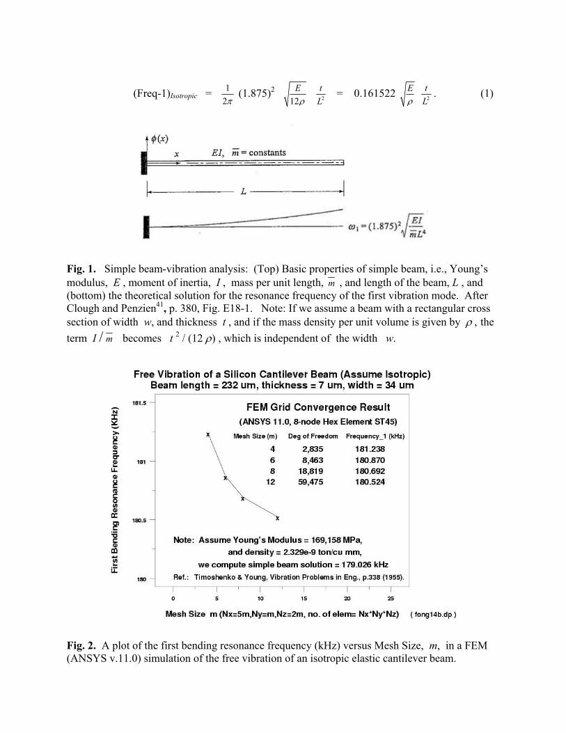
Fig. 1. Simple beam-vibration analysis: (Top) Basic properties of simple beam, i.e., Young’s
modulus, E , moment of inertia, I , mass per unit length, m , and length of the beam, L , and
(bottom) the theoretical solution for the resonance frequency of the first vibration mode. After
Clough and Penzien41
, p. 380, Fig. E18-1. Note: If we assume a beam with a rectangular cross
section of width w, and thickness t , and if the mass density per unit volume is given by t"."the
term I / m becomes t 2 / (12 t) , which is independent of the width w.
Fig. 2. A plot of the first bending resonance frequency (kHz) versus Mesh Size, m, in a FEM
(ANSYS v.11.0) simulation of the free vibration of an isotropic elastic cantilever beam.
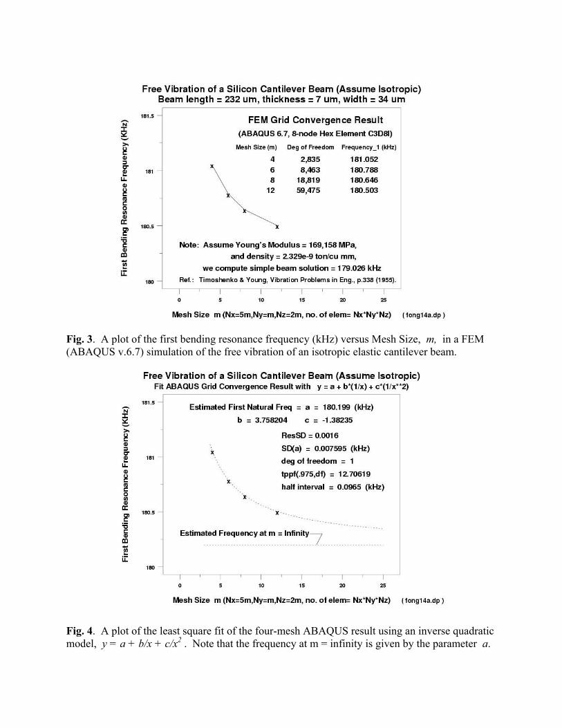
Fig. 3. A plot of the first bending resonance frequency (kHz) versus Mesh Size, m, in a FEM
(ABAQUS v.6.7) simulation of the free vibration of an isotropic elastic cantilever beam.
Fig. 4. A plot of the least square fit of the four-mesh ABAQUS result using an inverse quadratic
model, y = a + b/x + c/x2 . Note that the frequency at m = infinity is given by the parameter a.
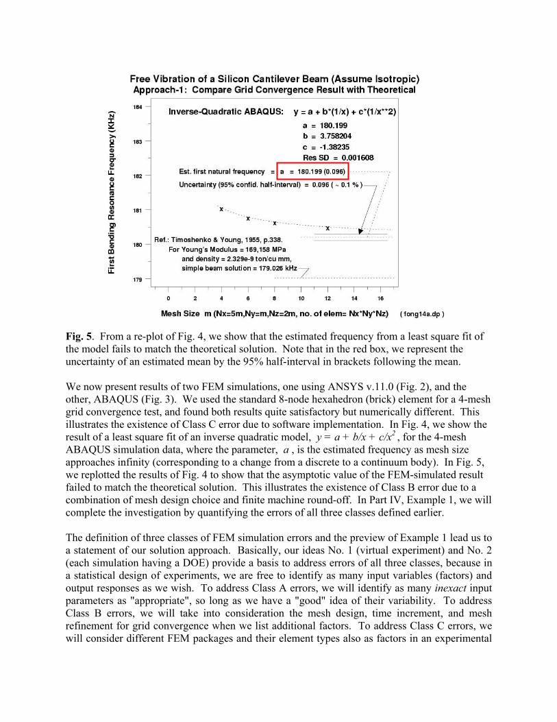
Fig. 5. From a re-plot of Fig. 4, we show that the estimated frequency from a least square fit of
the model fails to match the theoretical solution. Note that in the red box, we represent the
uncertainty of an estimated mean by the 95% half-interval in brackets following the mean.
We now present results of two FEM simulations, one using ANSYS v.11.0 (Fig. 2), and the
other, ABAQUS (Fig. 3). We used the standard 8-node hexahedron (brick) element for a 4-mesh
grid convergence test, and found both results quite satisfactory but numerically different. This
illustrates the existence of Class C error due to software implementation. In Fig. 4, we show the
result of a least square fit of an inverse quadratic model, y = a + b/x + c/x2 , for the 4-mesh
ABAQUS simulation data, where the parameter, a , is the estimated frequency as mesh size
approaches infinity (corresponding to a change from a discrete to a continuum body). In Fig. 5,
we replotted the results of Fig. 4 to show that the asymptotic value of the FEM-simulated result
failed to match the theoretical solution. This illustrates the existence of Class B error due to a
combination of mesh design choice and finite machine round-off. In Part IV, Example 1, we will
complete the investigation by quantifying the errors of all three classes defined earlier.
The definition of three classes of FEM simulation errors and the preview of Example 1 lead us to
a statement of our solution approach. Basically, our ideas No. 1 (virtual experiment) and No. 2
(each simulation having a DOE) provide a basis to address errors of all three classes, because in
a statistical design of experiments, we are free to identify as many input variables (factors) and
output responses as we wish. To address Class A errors, we will identify as many inexact input
parameters as "appropriate", so long as we have a "good" idea of their variability. To address
Class B errors, we will take into consideration the mesh design, time increment, and mesh
refinement for grid convergence when we list additional factors. To address Class C errors, we
will consider different FEM packages and their element types also as factors in an experimental
design. We will, of course, end up with a large number of factors, but by using fractional
factorial design of two-level experiments, we can reduce the number of computer runs to a
manageable size in order to estimate uncertainty as a prediction 95% confidence interval.
Part II. Topic A: Fundamentals of DOE (see Croarkin, et al39
, Chap. 5, Sect. 5.1, pp. 9-20)
In an experiment, we change one or more process variables (factors) in order to observe the
effect the changes have on one or more response variables. DOE is an efficient procedure for
planning experiments so that the data obtained can be analyzed to yield valid and objective
conclusions.
DOE begins with determining the objectives of an experiment and selecting the process factors
for the study. An Experimental Design is the laying out of a detailed experimental plan in
advance of doing the experiment. Well chosen experimental designs maximize the amount of
"information" that can be obtained for a given amount of experimental effort.
The statistical theory underlying DOE begins with the concept of process models. A process
model of the 'black box' type is formulated with several discrete or continuous input factors that
can be controlled, and one or more measured output responses. The output responses are
assumed continuous. Real or virtual experimental data are used to derive an empirical
(approximate) model linking the outputs and inputs. These empirical models generally contain
first-order (linear) and second-order (quadratic) terms.
The most common empirical models fit to the experimental data take either a first- or second-
order form. A first-order model with three factors, X1, X2 and X3, can be written as
Y = d2""-"d3X1 + d2X2 + d3X3 + d12X1X2 + d13X1X3 + d23X2X3 + errors (2)
Here, Y is the response for given levels of the main effects X1, X2 and X3, and the X1X2 ,
X1X3 , X2X3 terms are included to account for a possible interaction effect between X1 and X2 ,
X1 and X3 , X2 and X3 , respectively. The constant d0 is the response of Y when both main
effects are 0. In Example 1, we use a linear model with three factors and one response variable,
and a complete representation of that model contains just 8 terms on the right hand side of eq.
(2), i.e., a constant term, three main effects terms, three two-way interaction terms and one three-
way interaction term. In Example 2, we use a linear model with five factors and one response
variable, and total number of terms on the right hand side of eq. (2) is 25 , or 32.
A second-order (quadratic) model (typically used in response surface DOE's with suspected
curvature42
) does not include the three-way interaction term but adds three more terms to the
first-order model (2), namely
Note: Clearly, a full model could include many cross-product (or interaction) terms involving
squared X's. However, in general these terms are not needed and most DOE software defaults to
leaving them out of the model.
This concludes Section 5.1.1 of Croarkin, et al39
on "What is experimental design?" The reader
is invited to read Croarkin, et al39
for the two follow-up sections, namely, Section 5.1.2 on "What
are the uses of DOE?" and Section 5.1.3 on "What are the steps of DOE?"
Topic B: Assumptions of model building (see Croarkin, et al39
, Chap. 5, Sect. 5.2, pp. 21-34)
In all model building we make assumptions, and we also require certain conditions to be
approximately met for purposes of estimation. In Section 5.2 of Croarkin, et al39
, we look at
some of the engineering and mathematical assumptions we typically make. These are:
(a) Are the measurement systems capable for all of your responses?
(b) Is your process stable?
(c) Are your responses likely to be approximated well by simple polynomial models?
(d) Are the residuals (the difference between the model predictions and the actual
observations) well behaved?
Again, the reader is invited to read Croarkin, et al39
for more on this topic.
Topic C: Setting objectives for an experiment (see Croarkin, et al39
, Chap. 5, Sect. 5.3.1)
The objectives of an experiment are best determined by a team discussion. All of the objectives
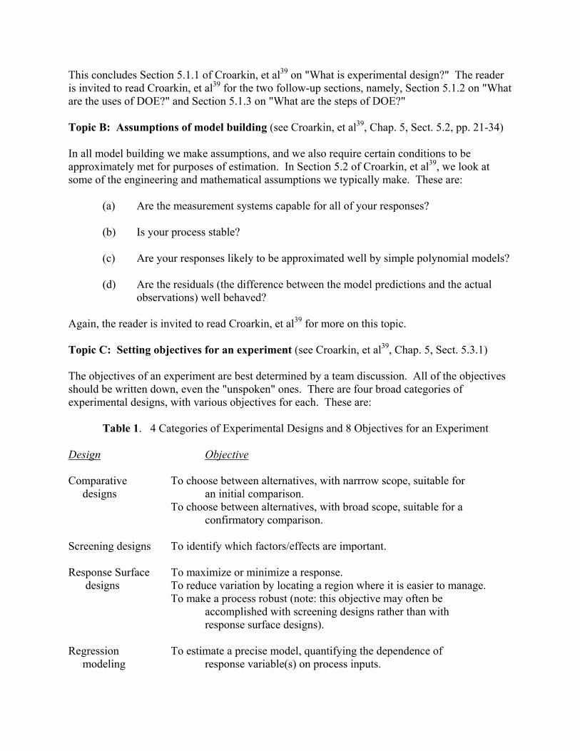
should be written down, even the "unspoken" ones. There are four broad categories of
experimental designs, with various objectives for each. These are:
Table 1. 4 Categories of Experimental Designs and 8 Objectives for an Experiment
Design Objective
Comparative To choose between alternatives, with narrrow scope, suitable for
designs an initial comparison.
To choose between alternatives, with broad scope, suitable for a
confirmatory comparison.
Screening designs To identify which factors/effects are important.
Response Surface To maximize or minimize a response.
designs To reduce variation by locating a region where it is easier to manage.
To make a process robust (note: this objective may often be
accomplished with screening designs rather than with
response surface designs).
Regression To estimate a precise model, quantifying the dependence of
modeling response variable(s) on process inputs.
Topic D: Selecting variables (factors and responses) (see Ref. 39, Sect. 5.3.2, pp. 39-41)
Process variables include both inputs (factors) and outputs (responses). The selection of these
variables is best done as a team effort. The team should
(a) Include all important factors (based on engineering judgment).
(b) Be bold, but not foolish, in choosing the low and high factor levels.
(c) Check the factor settings for impractical or impossible combinations, such as very
low pressure and very high gas flows.
(d) Include all relevant responses.
(e) Avoid using only responses that combine two or more measurements of the
process. For example, if interested in selectivity (the ratio of two etch rates),
measure both rates, not just the ratio.
We have to choose the range of the settings for input factors, and it is wise to give this some
thought beforehand rather than just try extreme values. In some cases, extreme values will give
runs that are not feasible; in other cases, extreme ranges might move one out of a smooth area of
the response surface into some jagged region, or close to an asymptote.
The most popular experimental designs are two-level designs. Why only two levels? There are a
number of good reasons why two is the most common choice amongst engineers; one reason is
that it is ideal for screening designs, simple and economical; it also gives most of the information
required to go to a multilevel response surface experiment if one is needed.
The standard layout for a 2-level design uses +1 and -1 notation to denote the "high level" and
the "low level" respectively, for each factor. For example, the matrix below
Factor 1 (X1) Factor 2 (X2)
Trial 1 -1 -1
Trial 2 +1 -1
Trial 3 -1 +1
Trial 4 +1 -1
describes an experiment in which 4 trials (or runs) were conducted with each factor set to high or
low during a run according to whether the matrix had a +1 or -1 set for the factor during that
trial. If the experiment had more than 2 factors, there would be an additional column in the
matrix for each additional factor. Note: An alternative convention is to shorten the matrix
notation for a two-level design by just recording the plus and minus signs, leaving out the "1's".
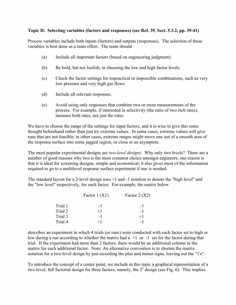
To introduce the concept of a center point, we include in this topic a graphical representation of a
two-level, full factorial design for three factors, namely, the 23 design (see Fig. 6). This implies
eight runs (not counting replications or center point runs). The arrows show the direction of
increase of the factors. The numbers '1' through '8' at the corners of the design box reference the
"Standard Order" of runs (also referred to as the "Yates Order").
Fig. 6. A 23 two-level, full factorial design; factors X1, X2, X3.
As mentioned earlier, we adopt the convention of +1 and -1 for the factor settings of a two-level
design. When we include a center point during the experiment, we mean a point located in the
middle of the design cube, and the convention is to denote a center point by the value "0". For a
more detailed exposition of the two-level design, the reader is invited to read the remaining
pages of Ref. 39, Chap. 5, Section 5.3.2, pp. 39-41.
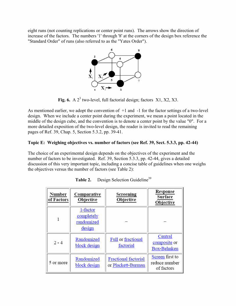
Topic E: Weighing objectives vs. number of factors (see Ref. 39, Sect. 5.3.3, pp. 42-44)
The choice of an experimental design depends on the objectives of the experiment and the
number of factors to be investigated. Ref. 39, Section 5.3.3, pp. 42-44, gives a detailed
discussion of this very important topic, including a concise table of guidelines when one weighs
the objectives versus the number of factors (see Table 2):
Table 2. Design Selection Guideline39

Table 2 refers to a number of designs that are well-known as a subset of a much larger set of
designs available in the literature as enumerated below:
Design Type 1. Completely randomized designs.
Design Type 2. Randomized block designs, which include Latin squares, Graeco-Latin
squares, and Hyper-Graeco-Latin squares.
Design Type 3. Full factorial designs, which include two-level full factorial designs,
three-level full factorial designs, and a discussion of the blocking of full
factorial designs.
Design Type 4. Fractional factorial designs.
Design Type 5. Plackett-Burman designs.
Design Type 6. Response surface (second-order) designs, which include central composite
designs, Box-Behnken designs, and blocking a response surface design.
Design Type 7. Adding center points.
Design Type 8. Three-level, mixed level and fractional factorial designs.
Design Type 9. D-Optimal designs.
Design Type 10. Taguchi designs.
Design Type 11. John's ¾ fractional factorial designs.
Design Type 12. Small composite designs.
Design Type 13. Mixture designs, which include simplex-lattice designs, simplex-centroid
designs, and constrained mixture designs.
We refer the reader to Ref. 39, Chapter 5, for a detailed study of those types. It is a good idea to
choose a design that requires somewhat fewer runs than the budget permits, so that center point
runs can be added to check for curvature in a 2-level screening design and backup resources are
available to redo runs that have processing mishaps.
Part III. Application of a DOE Approach to FEM Simulations.
For an application of the DOE approach to FEM simulations, we choose the screening objective
and a two-level fractional factorial design that is applicable to any number of factors larger than
1 (see Table 2). The availability of (a) a public-domain statistical analysis software package
named DATAPLOT1, and (b) the documentation of an exploratory data analysis (EDA) approach
of DATAPLOT for analyzing the data in 10 steps from a designed experiment (see Croarkin, et
al39
, Chap. 5, Section 5.5.9, pp. 313-412), made it possible for us to implement a specific
application of the proposed DOE approach to FEM-based simulations.
Let us introduce the so-called EDA approach of DATAPLOT to a screening problem in
experimental design and its 10-step algorithm. In general, there are two characteristics of a
screening problem: (a) There are many factors to consider. (b) Each of these factors may be
either continuous or discrete. The desired output from the analysis of a screening problem is:
1. A ranked list (by order of importance) of factors.
2. The best settings for each of the factors.
3. A good model.
4. Insight.
The essentials of the screen problem are:
1. There are k factors with n observations.
2. The generic model is
Y = f (X1, X2, ..., Xk) (3)
In particular, the EDA approach implemented in DATAPLOT is applied to 2k full factorial and
2k-p
fractional factorial designs. Let us introduce a 10-step EDA process for analyzing the data
from 2k full factorial and 2
k-p fractional factorial designs as follows: (Note: For consistency
with Ref. [39] in which DOE was replaced by DEX as an abbreviation for design of experiments,
we list below the titles of each step with a joint abbreviation, DOE/DEX .)
Step 1. Ordered data plot.
Step 2. DOE/DEX scatter plot.
Step 3. DOE/DEX mean plot.
Step 4. Interaction effects matrix plot.
Step 5. Block plot.
Step 6. DOE/DEX Youden plot.
Step 7. |Effects| plot.
Step 8. Half-normal probability plot.
Step 9. Cumulative residual standard deviation plot.
Step 10. DOE/DEX contour plot of two dominant factors.
Each of these plots will be presented with the following format:
1. Purpose of the plot.
2. Output of the plot.
3. Definition of the plot.
4. Motivation for the plot.
5. An example of the plot.
6. A discussion of how to interpret the plot.
7. Conclusions we can draw from the plot for the example data.
Part IV. Two Examples
Example 1. Free Vibration of an Isotropic Elastic Cantilever Beam
For a free vibration problem of an isotropic elastic cantilever beam, let us denote the length of
the beam by L. Assuming the beam has a rectangular cross-section of width w, and thickness t,
we denote the two material property constants of the beam by E, itsYoung's modulus, and p. Poisson's ratio. Let the density of the beam be deonted by t"0"As shown in Part I, eq. (1), it is
known40,41
that the first bending resonance frequency of such beam depends only on four of its
six parameters, namely, L, t, E, and t .
Motivated by an application in atomic force microscopy where a cantilever beam is made of
silicon, and adopting the SI units of mm, ton, s, N, and MPa, we assign the values of the four
parameters as follows: L = 0.232, t = 0.007, E = 169,158, and t"= 2.329e-09. Let Y be the
response variable of the problem, i.e., the resonance frequency of the first bending mode of the
free vibration of the cantilever beam, we apply eq. (1) to compute that Y = 179.026 kHz.
For this example of FEM simulations, we shall use two commercially-available packages,
namely, ABAQUS4, version 6.7, and ANSYS
5, version 11.0. For each package, we shall use an
8-node brick (hexahedron) as the basic element. Considering a Cartesian coordinate system
where the length, thickness, and width of the beam are oriented in the x, y, and z directions,
respectively, and assuming the beam is uniformly subdivided into brick elements, we define Nx,
Ny, Nz as the number of subdivisions in x, y, and z directions, respectively. Let m be a positive
integer that denotes the size of a mesh design, and for this example, we shall adopt a specific
design such that Nx = 5m, Ny = m, and Nz = 2m. Thus the total number of elements for this
class of design is 10 m3. As m increases, the mesh is progressively refined such that the
discretized finite element model approaches a continuum as m approaches infinity. As shown
in Table 3 showing the FEM results presented earlier in Part I, Figs. 2 through 5, the frequency
estimated from a 4-mesh grid convergence technique fails to match the theoretical solution.
Table 3. 4-Mesh Simulation Results and Grid Convergence Estimates of FEM Uncertainty
Mesh No. of No. of Degrees of Y (kHz) Y (kHz)
size elements nodes freedom (ABAQUS) (ANSYS)
---------------------------------------------------------------------------------------------------------
4 640 945 2,835 181.052 181.238
6 2,160 2,821 8,463 180.788 180.870
8 5,120 6,273 18,819 180.646 180.692
12 17,280 19,825 59,475 180.503 180.524
infinity (via a least square fit, Figs. 4 and 5) .. 180.199 (0.096) 180.201 (0.081)
In short, this example illustrates that, because of additional errors such as round-off and matrix
solver routines that have not been accounted for, there is always the difficulty of using a grid
convergence technique to progressively refine the mesh of a discretized model to the "correct"
limit of a continuum. At best, we use a least square approximation technique in this exercise to
estimate the so-called Class B errors due to spatial discretization. For ABAQUS simulation, that
Example 1 - Continued
error is 180.199 - 179.026 = 1.173 kHz, or about 0.66 %, and the same is true for the ANSYS
simulation, even though the two simulations do not seem to be identical. Without knowing a
theoretical solution, the only uncertainty we can calculate using the grid convergence method is
the prediction 95% confidence half-interval, which is 0.096 kHz or 0.081 kHz, for ABAQUS or
ANSYS simulations, respectively. This ends our investigation for Class B error (mathematical).
We now turn our attention to a method to address both Class A and Class C errors. For this, we
introduce our new approach by using the method of DOE. Our first step is to construct a table of
factors and their two-level variabilities. As shown in Fig. 6, a 3-factor 2-level DOE needs 8 runs
for a full-factorial, and only 4 runs for a half-factorial design. We plan to use both designs in
this example to gain some valuable insight into the difference between those two designs. The
center point around which we choose to conduct the 8-run and 4-run experiments is the FEM
simulation result at a single mesh size, namely, m = 4. Since mass density can be measured
quite precisely and has negligible variability, we choose to work with the other three factors,
namely, the length, L, thickness, t, and Young's modulus, E. Based on laboratory experience32
on the measurement variability of those three factors, we construct Table 4 for the first step of a
DOE exercise:
Table 4 Factors and Two-Level Variability in DOE
Factor Center Point Value Percent Change32
( +1 ) ( -1 )
------------------------------------------------------------------------------------------------
X1 = L 0.232 mm 1.6 % 0.23571 0.22829
X2 = t 0.007 mm 2.5 % 0.00718 0.00682
X3 = E 169,158 MPa 0.1 % 169,327 168,989
In Table 5, we show the 8-run FEM simulation results and the full-factorial DOE with which we
conducted simulations in both ABAQUS and ANSYS. Using a DATAPLOT subroutine for a
10-step analysis of DOE data presented in Part III, we first examine the output results for the 8-
run ABAQUS data as shown in 5 of its 10 plots given by Figs. 7 through 11.
Table 5. ABAQUS 8-run Results for a Full-Factorial Two-Level Design
Order of Run X1 X2 X3 ABAQUS (kHz) ANSYS (kHz)
--------------------------------------------------------------------------------------------------
1 -1 -1 -1 182.119 182.306
2 +1 -1 -1 170.807 170.981
3 -1 +1 -1 191.692 191.888
4 +1 +1 -1 179.786 179.970
5 -1 -1 +1 182.301 182.488
6 +1 -1 +1 170.977 171.152
7 -1 +1 +1 191.883 192.080
8 +1 +1 +1 179.966 180.150
Example 1 -
Continued
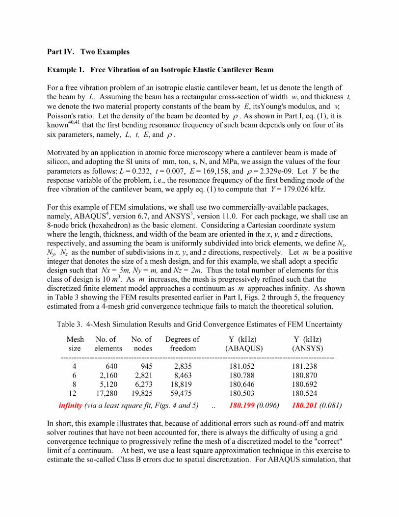
Fig. 7 First of ten plots by DATAPLOT showing the ABAQUS data as an ordered set. Note the
table at the bottom of the plot being the transposed DOE matrix with re-ordered columns.
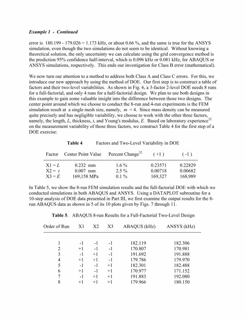
Fig. 8. Step 3 of a 10-step analysis of the ABAQUS data from 8 runs of experiments showing
the main effects of the full factorial 2-level design (k =3, n =8). Note X1 and X2 are dominant.
Example 1 -
Continued
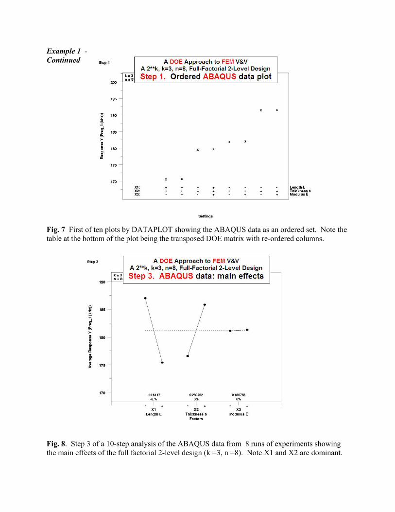
Fig. 9. Step 4 of a 10-step analysis of the ABAQUS data from 8 experimental runs showing the
interaction effects of the full factorial design (k =3, n =8). Note the lack of interaction effects.
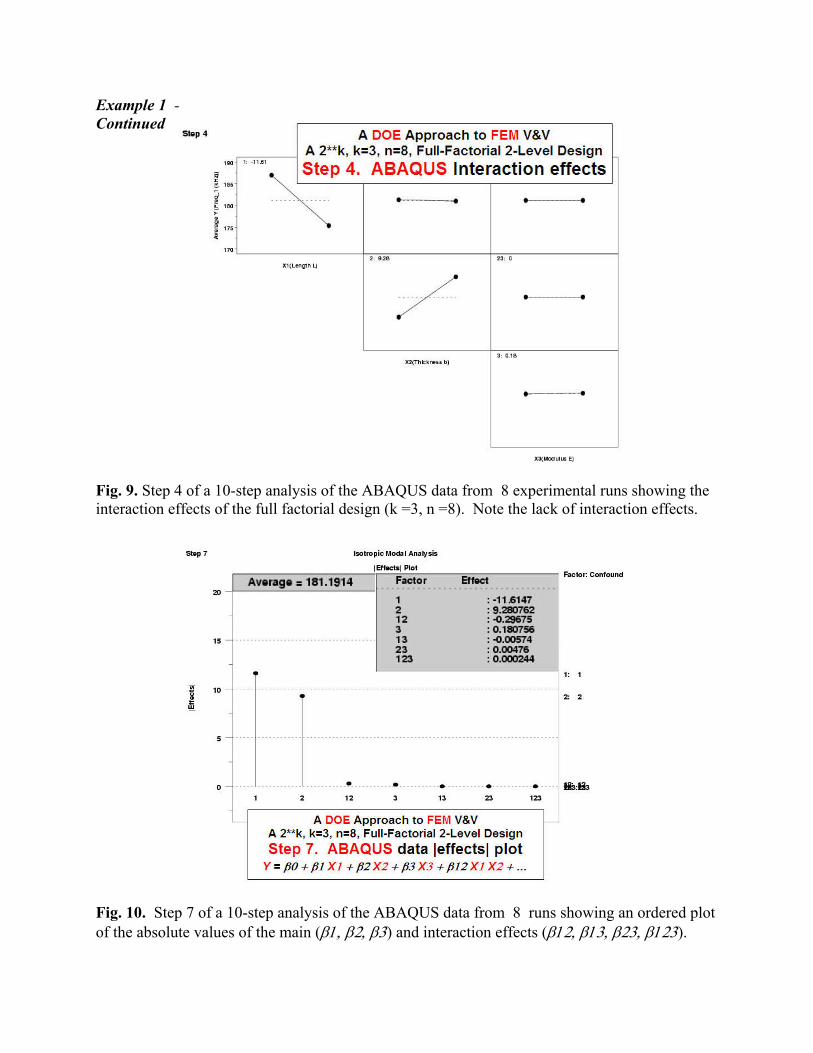
Fig. 10. Step 7 of a 10-step analysis of the ABAQUS data from 8 runs showing an ordered plot
of the absolute values of the main (d3."d4."d5) and interaction effects (d34."d35."d45."d345).
Example 1 -
Continued
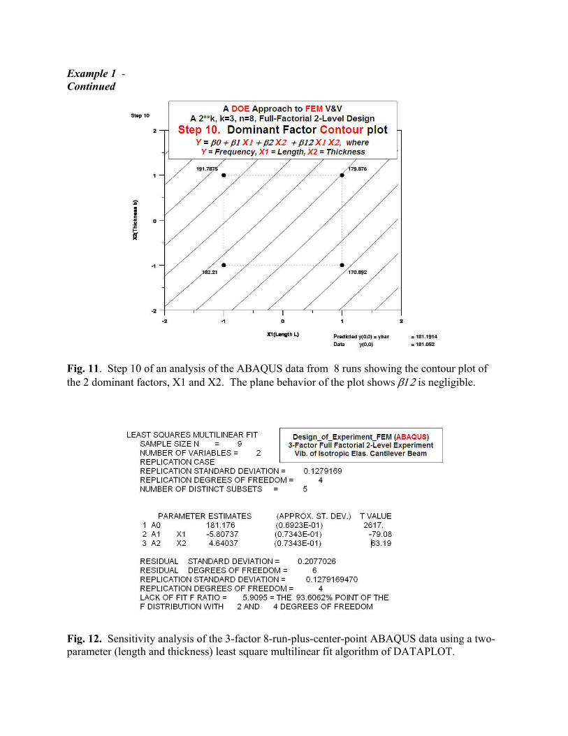
Fig. 11. Step 10 of an analysis of the ABAQUS data from 8 runs showing the contour plot of
the 2 dominant factors, X1 and X2. The plane behavior of the plot shows d34 is negligible.
Fig. 12. Sensitivity analysis of the 3-factor 8-run-plus-center-point ABAQUS data using a two-
parameter (length and thickness) least square multilinear fit algorithm of DATAPLOT.
Example 1 -
= 172.0788
= 190.273
= 171.587
= 190.765
Continued
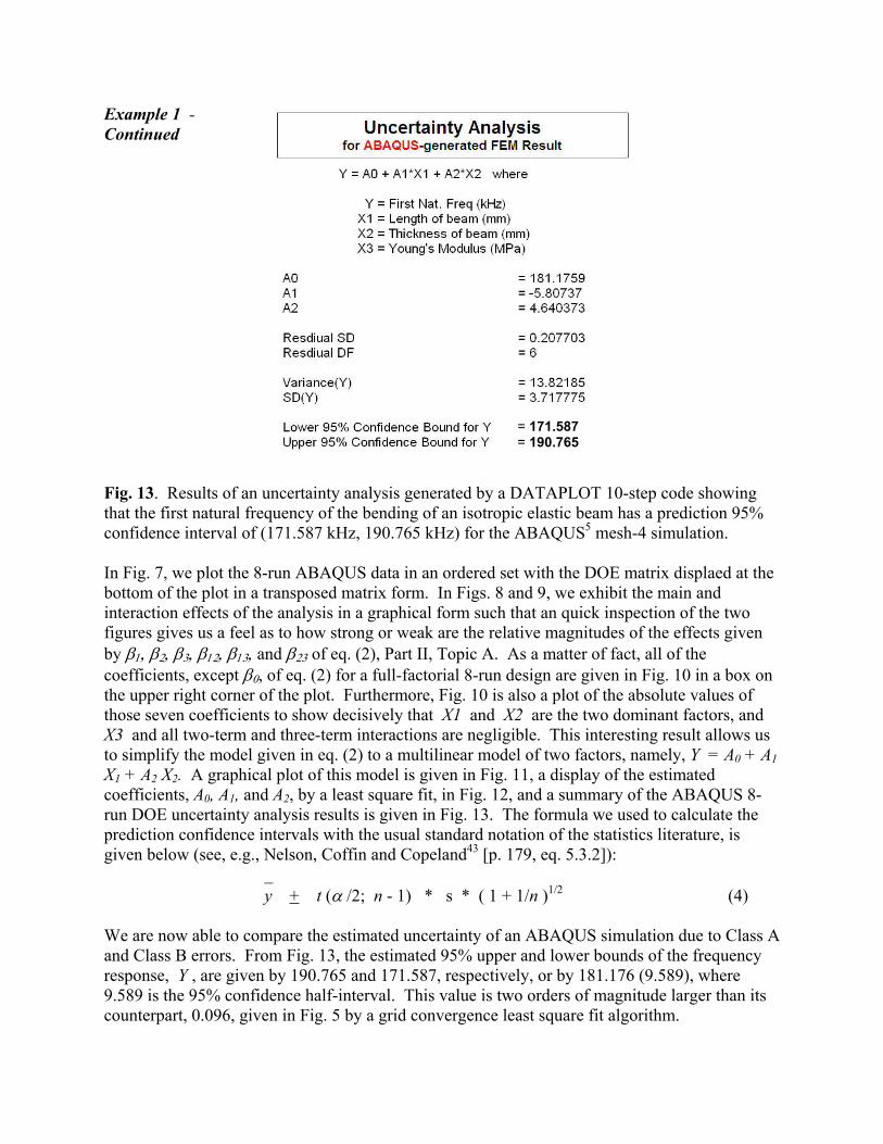
Fig. 13. Results of an uncertainty analysis generated by a DATAPLOT 10-step code showing
that the first natural frequency of the bending of an isotropic elastic beam has a prediction 95%
confidence interval of (171.587 kHz, 190.765 kHz) for the ABAQUS5 mesh-4 simulation.
In Fig. 7, we plot the 8-run ABAQUS data in an ordered set with the DOE matrix displaed at the
bottom of the plot in a transposed matrix form. In Figs. 8 and 9, we exhibit the main and
interaction effects of the analysis in a graphical form such that an quick inspection of the two
figures gives us a feel as to how strong or weak are the relative magnitudes of the effects given
by d3."d4."d5."d34."d35. and d45 of eq. (2), Part II, Topic A. As a matter of fact, all of the
coefficients, except d2, of eq. (2) for a full-factorial 8-run design are given in Fig. 10 in a box on
the upper right corner of the plot. Furthermore, Fig. 10 is also a plot of the absolute values of
those seven coefficients to show decisively that X1 and X2 are the two dominant factors, and
X3 and all two-term and three-term interactions are negligible. This interesting result allows us
to simplify the model given in eq. (2) to a multilinear model of two factors, namely, Y = A0 + A1
X1 + A2 X2. A graphical plot of this model is given in Fig. 11, a display of the estimated
coefficients, A0, A1, and A2, by a least square fit, in Fig. 12, and a summary of the ABAQUS 8-
run DOE uncertainty analysis results is given in Fig. 13. The formula we used to calculate the
prediction confidence intervals with the usual standard notation of the statistics literature, is
given below (see, e.g., Nelson, Coffin and Copeland43
[p. 179, eq. 5.3.2]):
_
y + t (c /2; n - 1) * s * ( 1 + 1/n )1/2
(4)
We are now able to compare the estimated uncertainty of an ABAQUS simulation due to Class A
and Class B errors. From Fig. 13, the estimated 95% upper and lower bounds of the frequency
response, Y , are given by 190.765 and 171.587, respectively, or by 181.176 (9.589), where
9.589 is the 95% confidence half-interval. This value is two orders of magnitude larger than its
counterpart, 0.096, given in Fig. 5 by a grid convergence least square fit algorithm.
Example 1 - Continued
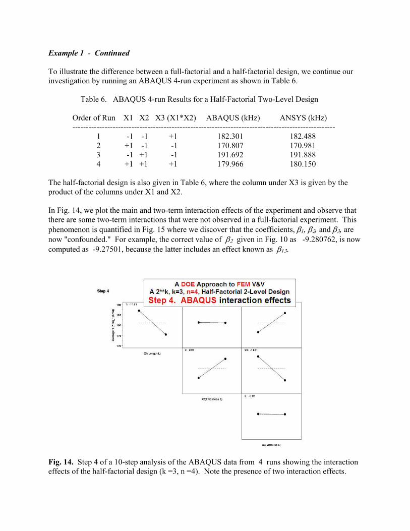
To illustrate the difference between a full-factorial and a half-factorial design, we continue our
investigation by running an ABAQUS 4-run experiment as shown in Table 6.
Table 6. ABAQUS 4-run Results for a Half-Factorial Two-Level Design
Order of Run X1 X2 X3 (X1*X2) ABAQUS (kHz) ANSYS (kHz)
--------------------------------------------------------------------------------------------------
1 -1 -1 +1 182.301 182.488
2 +1 -1 -1 170.807 170.981
3 -1 +1 -1 191.692 191.888
4 +1 +1 +1 179.966 180.150
The half-factorial design is also given in Table 6, where the column under X3 is given by the
product of the columns under X1 and X2.
In Fig. 14, we plot the main and two-term interaction effects of the experiment and observe that
there are some two-term interactions that were not observed in a full-factorial experiment. This
phenomenon is quantified in Fig. 15 where we discover that the coefficients, d3."d4."and d5. are
now "confounded." For example, the correct value of d4 given in Fig. 10 as -9.280762, is now
computed as -9.27501, because the latter includes an effect known as d35.
Fig. 14. Step 4 of a 10-step analysis of the ABAQUS data from 4 runs showing the interaction
effects of the half-factorial design (k =3, n =4). Note the presence of two interaction effects.
Example 1 -
Continued
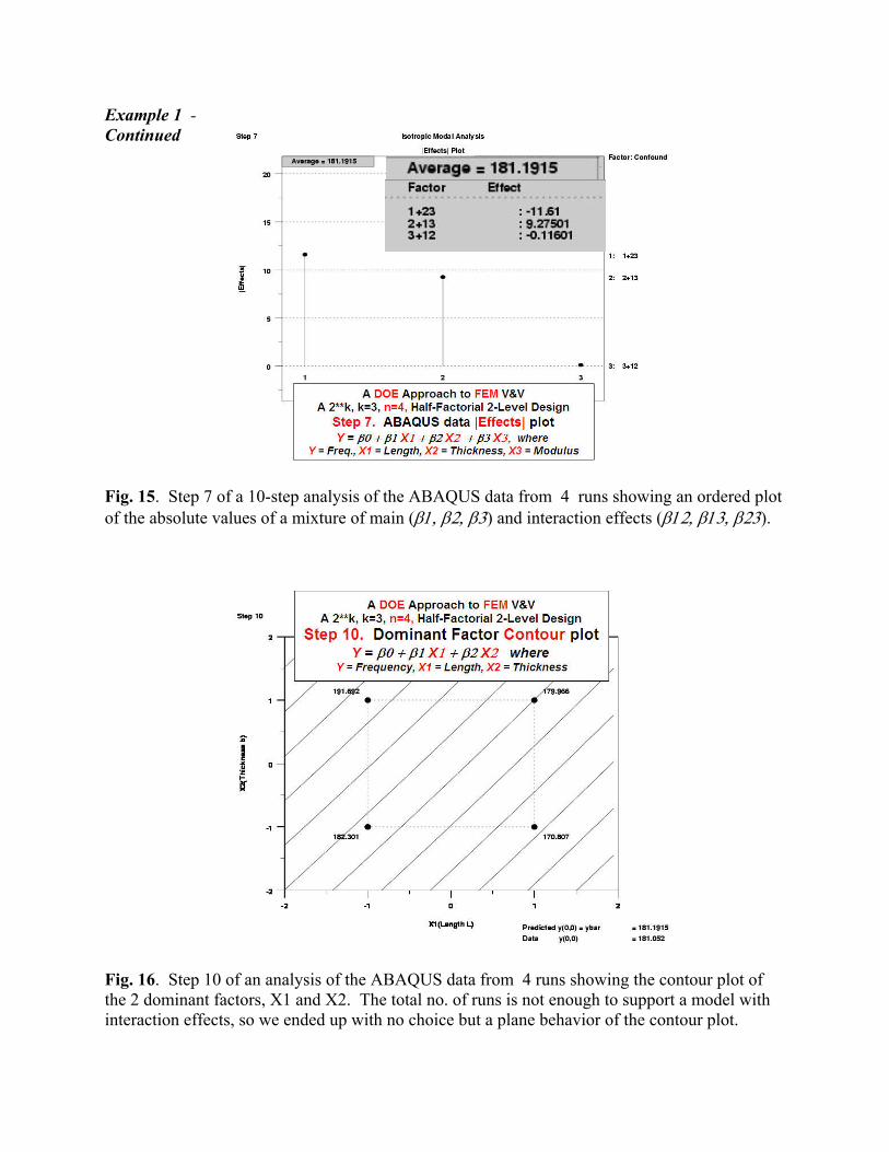
Fig. 15. Step 7 of a 10-step analysis of the ABAQUS data from 4 runs showing an ordered plot
of the absolute values of a mixture of main (d3."d4."d5) and interaction effects (d34."d35."d45).
Fig. 16. Step 10 of an analysis of the ABAQUS data from 4 runs showing the contour plot of
the 2 dominant factors, X1 and X2. The total no. of runs is not enough to support a model with
interaction effects, so we ended up with no choice but a plane behavior of the contour plot.
= 163.649
= 198.679
Example 1 -
Continued
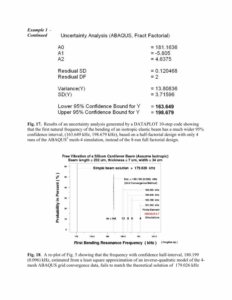
Fig. 17. Results of an uncertainty analysis generated by a DATAPLOT 10-step code showing
that the first natural frequency of the bending of an isotropic elastic beam has a much wider 95%
confidence interval, (163.649 kHz, 198.679 kHz), based on a half-factorial design with only 4
runs of the ABAQUS5 mesh-4 simulation, instead of the 8-run full factorial design.
Fig. 18. A re-plot of Fig. 5 showing that the frequency with confidence half-interval, 180.199
(0.096) kHz, estimated from a least square approximation of an inverse-quadratic model of the 4-
mesh ABAQUS grid convergence data, fails to match the theoretical solution of 179.026 kHz
Example 1 - Continued
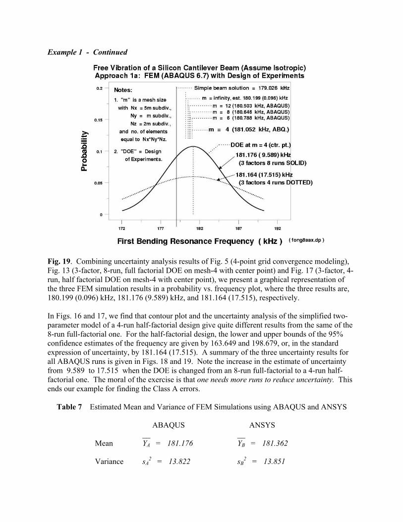
Fig. 19. Combining uncertainty analysis results of Fig. 5 (4-point grid convergence modeling),
Fig. 13 (3-factor, 8-run, full factorial DOE on mesh-4 with center point) and Fig. 17 (3-factor, 4-
run, half factorial DOE on mesh-4 with center point), we present a graphical representation of
the three FEM simulation results in a probability vs. frequency plot, where the three results are,
180.199 (0.096) kHz, 181.176 (9.589) kHz, and 181.164 (17.515), respectively.
In Figs. 16 and 17, we find that contour plot and the uncertainty analysis of the simplified two-
parameter model of a 4-run half-factorial design give quite different results from the same of the
8-run full-factorial one. For the half-factorial design, the lower and upper bounds of the 95%
confidence estimates of the frequency are given by 163.649 and 198.679, or, in the standard
expression of uncertainty, by 181.164 (17.515). A summary of the three uncertainty results for
all ABAQUS runs is given in Figs. 18 and 19. Note the increase in the estimate of uncertainty
from 9.589 to 17.515 when the DOE is changed from an 8-run full-factorial to a 4-run half-
factorial one. The moral of the exercise is that one needs more runs to reduce uncertainty. This
ends our example for finding the Class A errors.
Table 7 Estimated Mean and Variance of FEM Simulations using ABAQUS and ANSYS
ABAQUS ANSYS
__ __
Mean YA = 181.176 YB = 181.362 B
Variance sA2 = 13.822 sB
2 = 13.851
Example 1 -
Continued
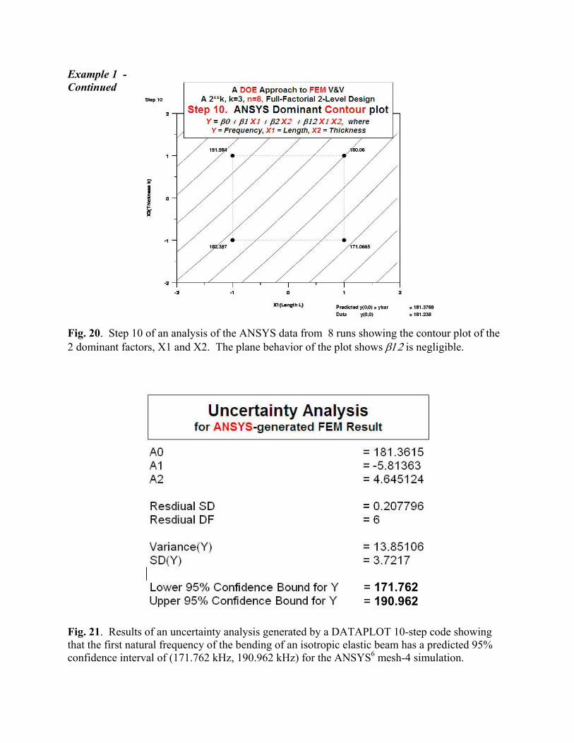
Fig. 20. Step 10 of an analysis of the ANSYS data from 8 runs showing the contour plot of the
2 dominant factors, X1 and X2. The plane behavior of the plot shows d34 is negligible.
= 171.762
= 190.962
Fig. 21. Results of an uncertainty analysis generated by a DATAPLOT 10-step code showing
that the first natural frequency of the bending of an isotropic elastic beam has a predicted 95%
confidence interval of (171.762 kHz, 190.962 kHz) for the ANSYS6 mesh-4 simulation.
Example 1 - Continued
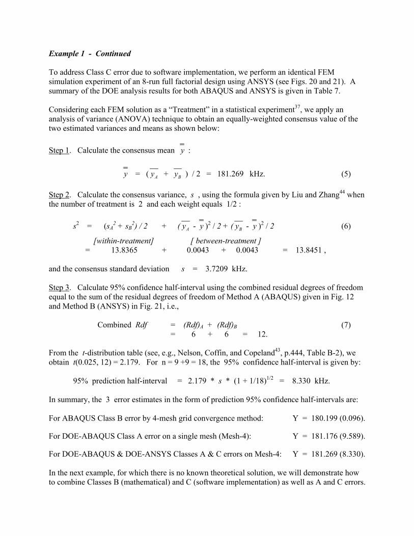
To address Class C error due to software implementation, we perform an identical FEM
simulation experiment of an 8-run full factorial design using ANSYS (see Figs. 20 and 21). A
summary of the DOE analysis results for both ABAQUS and ANSYS is given in Table 7.
Considering each FEM solution as a “Treatment” in a statistical experiment37
, we apply an
analysis of variance (ANOVA) technique to obtain an equally-weighted consensus value of the
two estimated variances and means as shown below:
Step 1. Calculate the consensus mean y :
y = ( Ay + By ) / 2 = 181.269 kHz. (5)
Step 2. Calculate the consensus variance, s , using the formula given by Liu and Zhang44
when
the number of treatment is 2 and each weight equals 1/2 :
s2 = (sA
2 + sB
2) / 2 + ( Ay - y )
2 / 2 + ( By - y )
2 / 2 (6)
[within-treatment] [ between-treatment ]
= 13.8365 + 0.0043 + 0.0043 = 13.8451 ,
and the consensus standard deviation s = 3.7209 kHz.
Step 3. Calculate 95% confidence half-interval using the combined residual degrees of freedom
equal to the sum of the residual degrees of freedom of Method A (ABAQUS) given in Fig. 12
and Method B (ANSYS) in Fig. 21, i.e.,
Combined Rdf = (Rdf)A + (Rdf)B (7)
= 6 + 6 = 12.
From the t-distribution table (see, e.g., Nelson, Coffin, and Copeland43
, p.444, Table B-2), we
obtain t(0.025, 12) = 2.179. For n = 9 +9 = 18, the 95% confidence half-interval is given by:
95% prediction half-interval = 2.179 * s * (1 + 1/18)1/2
= 8.330 kHz.
In summary, the 3 error estimates in the form of prediction 95% confidence half-intervals are:
For ABAQUS Class B error by 4-mesh grid convergence method: Y = 180.199 (0.096). For DOE-ABAQUS Class A error on a single mesh (Mesh-4): Y = 181.176 (9.589).
For DOE-ABAQUS & DOE-ANSYS Classes A & C errors on Mesh-4: Y = 181.269 (8.330).
In the next example, for which there is no known theoretical solution, we will demonstrate how
to combine Classes B (mathematical) and C (software implementation) as well as A and C errors.
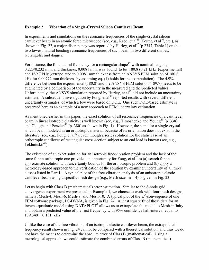
Example 2 Vibration of a Single-Crystal Silicon Cantilever Beam
In experiments and simulations on the resonance frequencies of the single-crystal silicon
cantilever beam in an atomic force microscope (see, e.g., Rabe, et al45
, Kester, et al46
, etc.), as
shown in Fig. 22, a major discrepancy was reported by Hurley, et al47
[p.2347, Table 1] on the
two lowest natural bending resonance frequencies of such beam in two different shapes,
rectangular and dagger.
For instance, the first natural frequency for a rectangular shape47
with nominal lengths,
0.223/0.232 mm, and thickness, 0.0081 mm, was found to be 180.8 (0.2) kHz (experimental)
and 189.7 kHz (extrapolated to 0.0081 mm thickness from an ANSYS FEM solution of 180.8
kHz for 0.00772 mm thickness by assuming eq. (1) holds for the extrapolation). The 4.9%
difference between the experimental (180.8) and the ANSYS FEM solution (189.7) needs to be
augmented by a comparison of the uncertainty in the measured and the predicted values.
Unfortunately, the ANSYS simulation reported by Hurley, et al47
did not include an uncertainty
estimate. A subsequent investigation by Fong, et al32
reported results with several different
uncertainty estimates, of which a few were based on DOE. One such DOE-based estimate is
presented here as an example of a new approach to FEM uncertainty estimation.
As mentioned earlier in this paper, the exact solution of all resonance frequencies of a cantilever
beam in linear isotropic elasticity is well known (see, e.g., Timoshenko and Young40
[p. 338],
and Clough and Penzien41
[p. 380] as shown in Fig. 1). However, the same for a single-crystal
silicon beam modeled as an orthotropic material because of its orientation does not exist in the
literature (see, e.g., Fong, et al32
), even though a series solution for the static case of an
orthotropic cantilever of rectangular cross-section subject to an end load is known (see, e.g.,
Lekhnitskii48
).
The existence of an exact solution for an isotropic free-vibration problem and the lack of the
same for an orthotropic one provided an opportunity for Fong, et al32
to (a) search for an
approximate solution with uncertainty bounds for the orthotropic problem and (b) apply a
metrology-based approach to the verification of the solution by examing uncertainty of all three
classes listed in Part I. A typical plot of the free vibration analysis of an anisotropic elastic
cantilever beam using a specific mesh design (e.g., Mesh size m = 4) is given in Fig. 23.
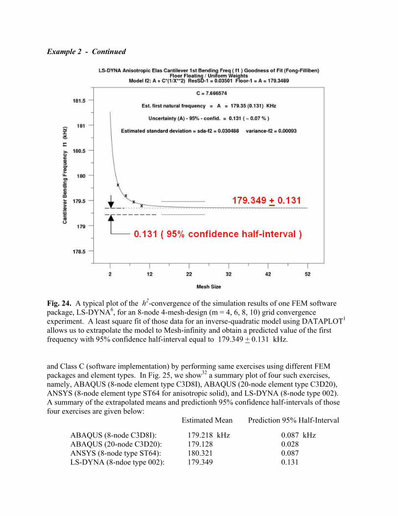
Let us begin with Class B (mathematical) error estimation. Similar to the 8-node grid
convergence experiment we presented in Example 1, we choose to work with four mesh designs,
namely, Mesh-4, Mesh-6, Mesh-8, and Mesh-10. A typical plot of the h2-convergence of one
FEM software package, LS-DYNA, is given in Fig. 24. A least square fit of those data for an
inverse-quadratic model using DATAPLOT1 allows us to extrapolate the model to Mesh-infinity
and obtain a predicted value of the first frequency with 95% confidence half-interval equal to
179.349 + 0.131 kHz.
Unlike the case of the free vibration of an isotropic elastic cantilever beam, the extrapolated
frequency result shown in Fig. 24 cannot be compared with a theoretical solution, and thus we do
not have the means to determine the absolute error of Class B (mathematical). Using a
metrological approach, we could estimate the combined errors of Class B (mathematical)
Example 2 - Continued
Fig. 22. Typical geometry of a single-crystal silicon cantilever beam with the location of a tip in
contact with the surface of a sample in an atomic force microscope (after Kester, Rabe,
Presmanes, Tailhades, and Arnold46
[p. 1277, Fig. 3] ).
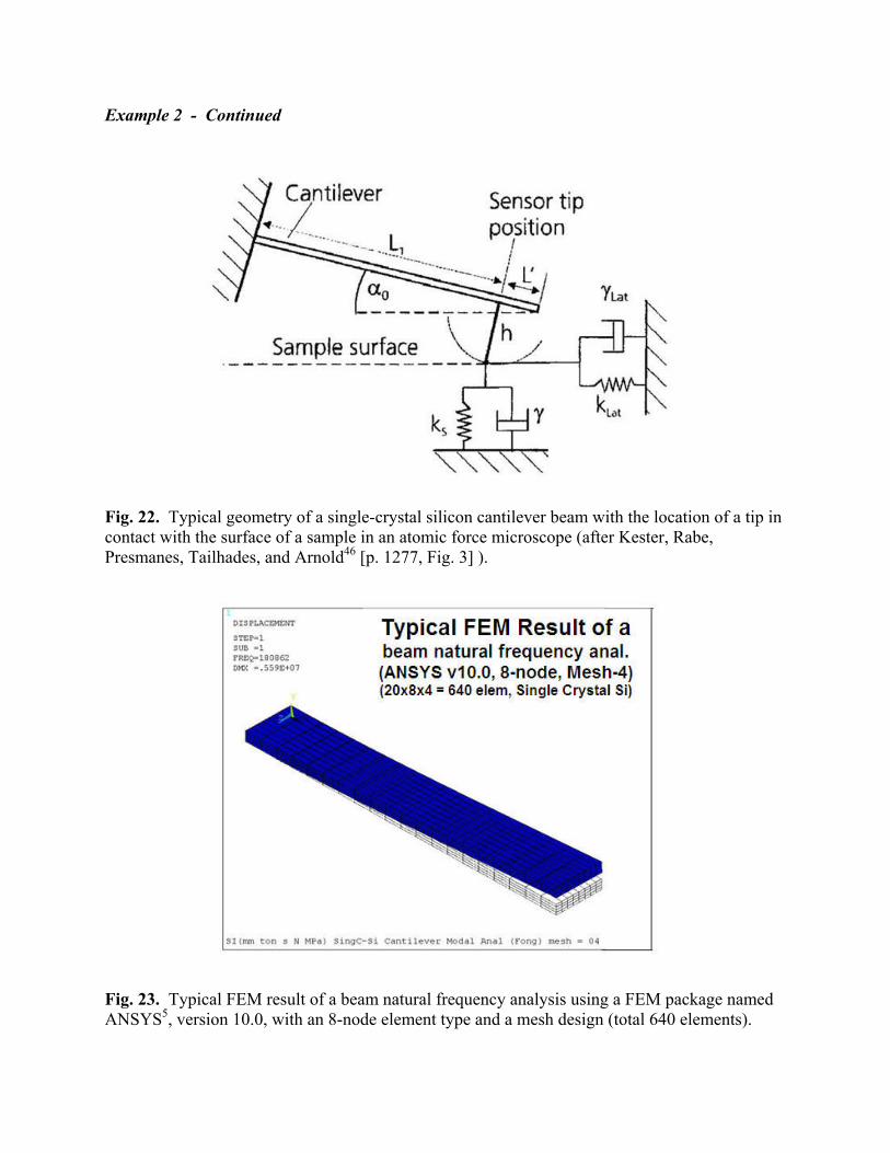
Fig. 23. Typical FEM result of a beam natural frequency analysis using a FEM package named
ANSYS5, version 10.0, with an 8-node element type and a mesh design (total 640 elements).
Example 2 - Continued
Fig. 24. A typical plot of the h2-convergence of the simulation results of one FEM software
package, LS-DYNA6, for an 8-node 4-mesh-design (m = 4, 6, 8, 10) grid convergence
experiment. A least square fit of those data for an inverse-quadratic model using DATAPLOT1
allows us to extrapolate the model to Mesh-infinity and obtain a predicted value of the first
frequency with 95% confidence half-interval equal to 179.349 + 0.131 kHz.
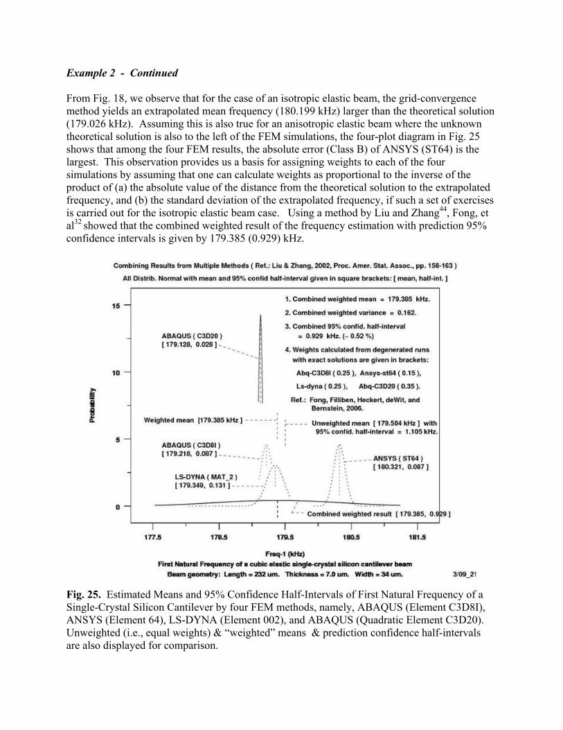
and Class C (software implementation) by performing same exercises using different FEM
packages and element types. In Fig. 25, we show32
a summary plot of four such exercises,
namely, ABAQUS (8-node element type C3D8I), ABAQUS (20-node element type C3D20),
ANSYS (8-node element type ST64 for anisotropic solid), and LS-DYNA (8-node type 002).
A summary of the extrapolated means and predictionh 95% confidence half-intervals of those
four exercises are given below:
Estimated Mean Prediction 95% Half-Interval
ABAQUS (8-node C3D8I): 179.218 kHz 0.087 kHz
ABAQUS (20-node C3D20): 179.128 0.028
ANSYS (8-node type ST64): 180.321 0.087
LS-DYNA (8-ndoe type 002): 179.349 0.131
Example 2 - Continued
From Fig. 18, we observe that for the case of an isotropic elastic beam, the grid-convergence
method yields an extrapolated mean frequency (180.199 kHz) larger than the theoretical solution
(179.026 kHz). Assuming this is also true for an anisotropic elastic beam where the unknown
theoretical solution is also to the left of the FEM simulations, the four-plot diagram in Fig. 25
shows that among the four FEM results, the absolute error (Class B) of ANSYS (ST64) is the
largest. This observation provides us a basis for assigning weights to each of the four
simulations by assuming that one can calculate weights as proportional to the inverse of the
product of (a) the absolute value of the distance from the theoretical solution to the extrapolated
frequency, and (b) the standard deviation of the extrapolated frequency, if such a set of exercises
is carried out for the isotropic elastic beam case. Using a method by Liu and Zhang44
, Fong, et
al32
showed that the combined weighted result of the frequency estimation with prediction 95%
confidence intervals is given by 179.385 (0.929) kHz.
Fig. 25. Estimated Means and 95% Confidence Half-Intervals of First Natural Frequency of a
Single-Crystal Silicon Cantilever by four FEM methods, namely, ABAQUS (Element C3D8I),
ANSYS (Element 64), LS-DYNA (Element 002), and ABAQUS (Quadratic Element C3D20).
Unweighted (i.e., equal weights) & “weighted” means & prediction confidence half-intervals
are also displayed for comparison.
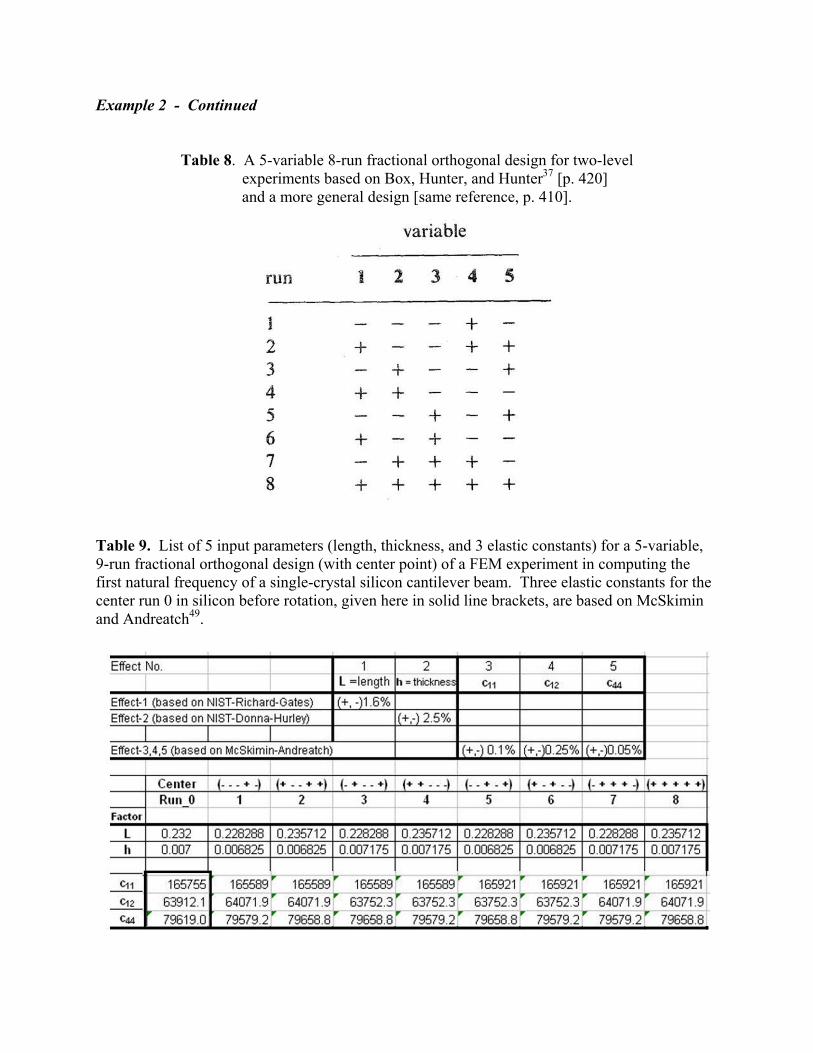
Example 2 - Continued
Table 8. A 5-variable 8-run fractional orthogonal design for two-level
experiments based on Box, Hunter, and Hunter37
[p. 420]
and a more general design [same reference, p. 410].
Table 9. List of 5 input parameters (length, thickness, and 3 elastic constants) for a 5-variable,
9-run fractional orthogonal design (with center point) of a FEM experiment in computing the
first natural frequency of a single-crystal silicon cantilever beam. Three elastic constants for the
center run 0 in silicon before rotation, given here in solid line brackets, are based on McSkimin
and Andreatch49
.
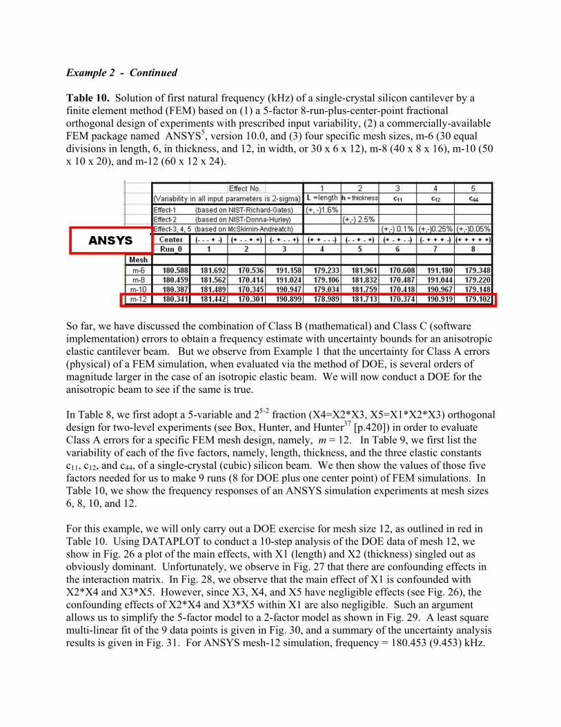
Example 2 - Continued
Table 10. Solution of first natural frequency (kHz) of a single-crystal silicon cantilever by a
finite element method (FEM) based on (1) a 5-factor 8-run-plus-center-point fractional
orthogonal design of experiments with prescribed input variability, (2) a commercially-available
FEM package named ANSYS5, version 10.0, and (3) four specific mesh sizes, m-6 (30 equal
divisions in length, 6, in thickness, and 12, in width, or 30 x 6 x 12), m-8 (40 x 8 x 16), m-10 (50
x 10 x 20), and m-12 (60 x 12 x 24).
So far, we have discussed the combination of Class B (mathematical) and Class C (software
implementation) errors to obtain a frequency estimate with uncertainty bounds for an anisotropic
elastic cantilever beam. But we observe from Example 1 that the uncertainty for Class A errors
(physical) of a FEM simulation, when evaluated via the method of DOE, is several orders of
magnitude larger in the case of an isotropic elastic beam. We will now conduct a DOE for the
anisotropic beam to see if the same is true.
In Table 8, we first adopt a 5-variable and 25-2
fraction (X4=X2*X3, X5=X1*X2*X3) orthogonal
design for two-level experiments (see Box, Hunter, and Hunter37
[p.420]) in order to evaluate
Class A errors for a specific FEM mesh design, namely, m = 12. In Table 9, we first list the
variability of each of the five factors, namely, length, thickness, and the three elastic constants
c11, c12, and c44, of a single-crystal (cubic) silicon beam. We then show the values of those five
factors needed for us to make 9 runs (8 for DOE plus one center point) of FEM simulations. In
Table 10, we show the frequency responses of an ANSYS simulation experiments at mesh sizes
6, 8, 10, and 12.
For this example, we will only carry out a DOE exercise for mesh size 12, as outlined in red in
Table 10. Using DATAPLOT to conduct a 10-step analysis of the DOE data of mesh 12, we
show in Fig. 26 a plot of the main effects, with X1 (length) and X2 (thickness) singled out as
obviously dominant. Unfortunately, we observe in Fig. 27 that there are confounding effects in
the interaction matrix. In Fig. 28, we observe that the main effect of X1 is confounded with
X2*X4 and X3*X5. However, since X3, X4, and X5 have negligible effects (see Fig. 26), the
confounding effects of X2*X4 and X3*X5 within X1 are also negligible. Such an argument
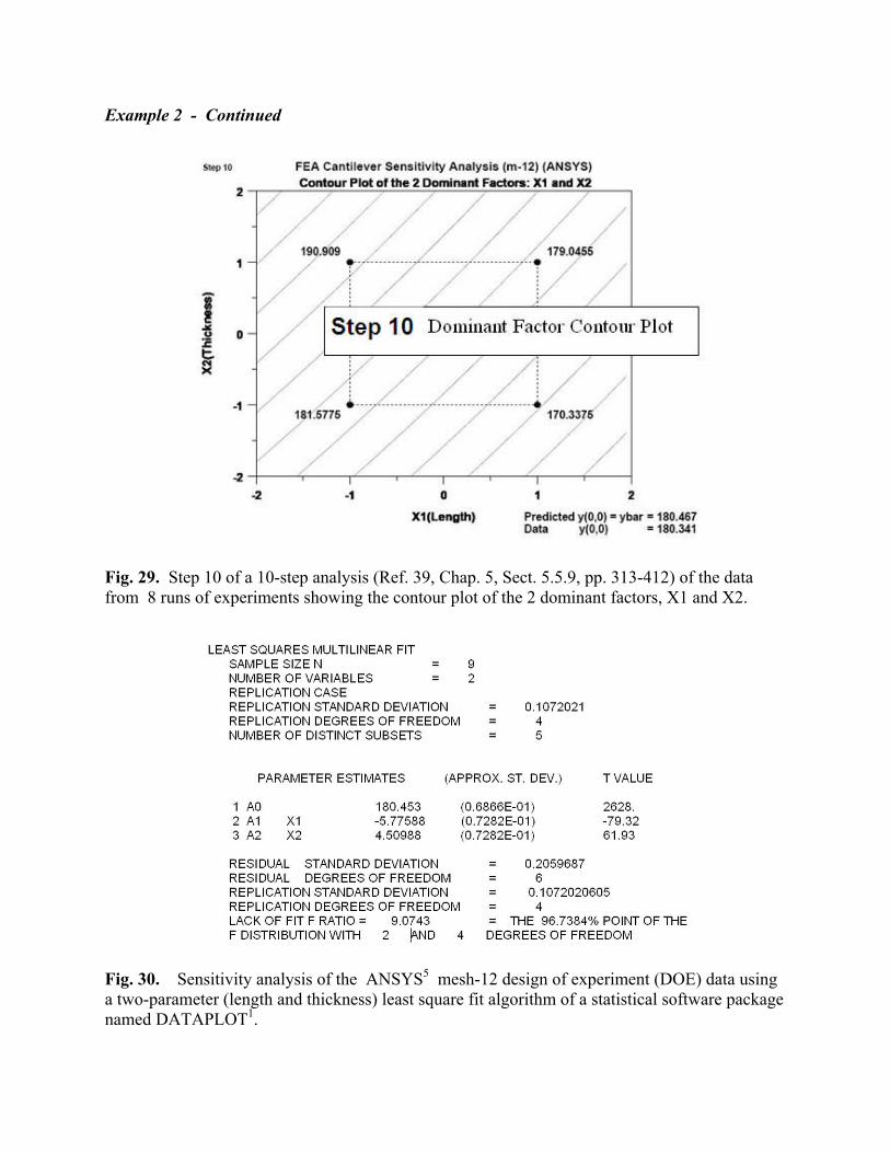
allows us to simplify the 5-factor model to a 2-factor model as shown in Fig. 29. A least square
multi-linear fit of the 9 data points is given in Fig. 30, and a summary of the uncertainty analysis
results is given in Fig. 31. For ANSYS mesh-12 simulation, frequency = 180.453 (9.453) kHz.
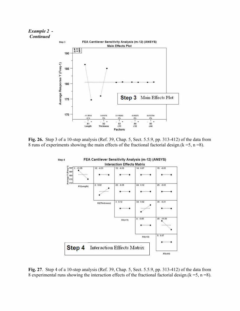
Example 2 -
Continued
Fig. 26. Step 3 of a 10-step analysis (Ref. 39, Chap. 5, Sect. 5.5.9, pp. 313-412) of the data from
8 runs of experiments showing the main effects of the fractional factorial design.(k =5, n =8).
Fig. 27. Step 4 of a 10-step analysis (Ref. 39, Chap. 5, Sect. 5.5.9, pp. 313-412) of the data from
8 experimental runs showing the interaction effects of the fractional factorial design.(k =5, n =8).
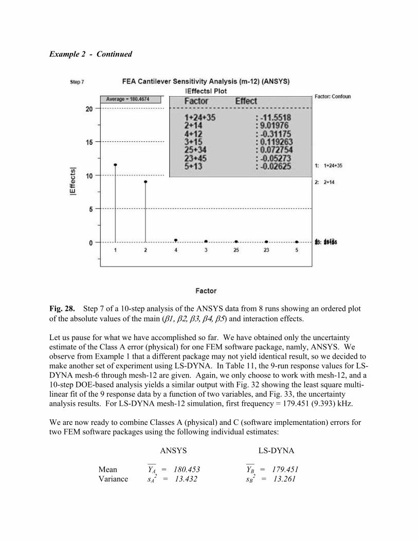
Example 2 - Continued
Fig. 28. Step 7 of a 10-step analysis of the ANSYS data from 8 runs showing an ordered plot
of the absolute values of the main (d3."d4."d5."d6."d7) and interaction effects.
Let us pause for what we have accomplished so far. We have obtained only the uncertainty
estimate of the Class A error (physical) for one FEM software package, namly, ANSYS. We
observe from Example 1 that a different package may not yield identical result, so we decided to
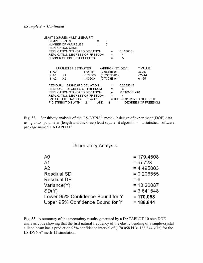
make another set of experiment using LS-DYNA. In Table 11, the 9-run response values for LS-
DYNA mesh-6 through mesh-12 are given. Again, we only choose to work with mesh-12, and a
10-step DOE-based analysis yields a similar output with Fig. 32 showing the least square multi-
linear fit of the 9 response data by a function of two variables, and Fig. 33, the uncertainty
analysis results. For LS-DYNA mesh-12 simulation, first frequency = 179.451 (9.393) kHz.
We are now ready to combine Classes A (physical) and C (software implementation) errors for
two FEM software packages using the following individual estimates:
ANSYS LS-DYNA
__ __
Mean YA = 180.453 YB = 179.451 B
Variance sA2 = 13.432 sB
2 = 13.261
Example 2 - Continued
Fig. 29. Step 10 of a 10-step analysis (Ref. 39, Chap. 5, Sect. 5.5.9, pp. 313-412) of the data
from 8 runs of experiments showing the contour plot of the 2 dominant factors, X1 and X2.
Fig. 30. Sensitivity analysis of the ANSYS5 mesh-12 design of experiment (DOE) data using
a two-parameter (length and thickness) least square fit algorithm of a statistical software package
named DATAPLOT1.
Example 2 - Continued
= 171.000
= 189.906
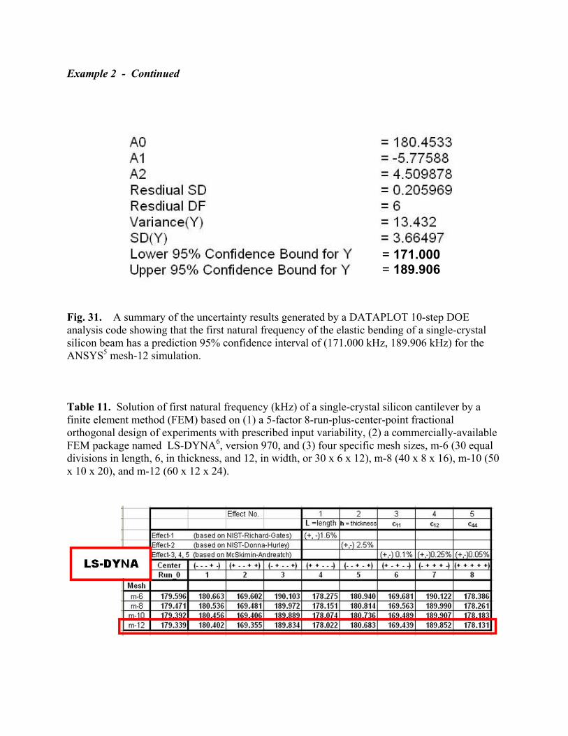
Fig. 31. A summary of the uncertainty results generated by a DATAPLOT 10-step DOE
analysis code showing that the first natural frequency of the elastic bending of a single-crystal
silicon beam has a prediction 95% confidence interval of (171.000 kHz, 189.906 kHz) for the
ANSYS5 mesh-12 simulation.
Table 11. Solution of first natural frequency (kHz) of a single-crystal silicon cantilever by a
finite element method (FEM) based on (1) a 5-factor 8-run-plus-center-point fractional
orthogonal design of experiments with prescribed input variability, (2) a commercially-available
FEM package named LS-DYNA6, version 970, and (3) four specific mesh sizes, m-6 (30 equal
divisions in length, 6, in thickness, and 12, in width, or 30 x 6 x 12), m-8 (40 x 8 x 16), m-10 (50
x 10 x 20), and m-12 (60 x 12 x 24).
Example 2 - Continued
Fig. 32. Sensitivity analysis of the LS-DYNA6 mesh-12 design of experiment (DOE) data
using a two-parameter (length and thickness) least square fit algorithm of a statistical software
package named DATAPLOT1.
= 170.058
= 188.844
Fig. 33. A summary of the uncertainty results generated by a DATAPLOT 10-step DOE
analysis code showing that the first natural frequency of the elastic bending of a single-crystal
silicon beam has a prediction 95% confidence interval of (170.058 kHz, 188.844 kHz) for the
LS-DYNA6 mesh-12 simulation.
Example 2 - Continued
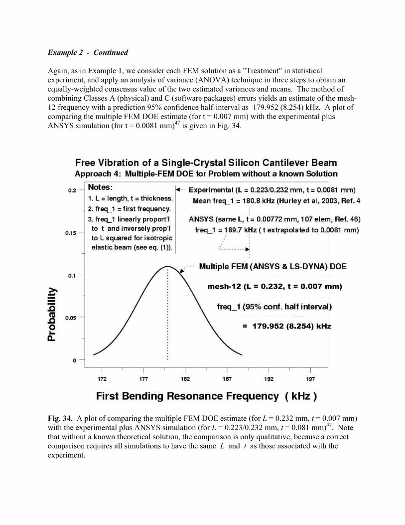
Again, as in Example 1, we consider each FEM solution as a "Treatment" in statistical
experiment, and apply an analysis of variance (ANOVA) technique in three steps to obtain an
equally-weighted consensus value of the two estimated variances and means. The method of
combining Classes A (physical) and C (software packages) errors yields an estimate of the mesh-
12 frequency with a prediction 95% confidence half-interval as 179.952 (8.254) kHz. A plot of
comparing the multiple FEM DOE estimate (for t = 0.007 mm) with the experimental plus
ANSYS simulation (for t = 0.0081 mm)47
is given in Fig. 34.
= 179.952 (8.254) kHz
mesh-12 (L = 0.232, t = 0.007 mm)
Fig. 34. A plot of comparing the multiple FEM DOE estimate (for L = 0.232 mm, t = 0.007 mm)
with the experimental plus ANSYS simulation (for L = 0.223/0.232 mm, t = 0.081 mm)47
. Note
that without a known theoretical solution, the comparison is only qualitative, because a correct
comparison requires all simulations to have the same L and t as those associated with the
experiment.
Significance and Limitations of the DOE Approach
The DOE approach to an uncertainty estimation of FEM simulations, as presented in this paper
with two examples, is significant for at least two reasons:
(1) It provides an alternative approach to uncertainty estimation of mathematical modeling
and simulation where the traditional approach of using Monte Carlo method becomes cost-
prohibitive as the degrees of freedom per simulation go as high as hundreds of thousands or more
in most FEM simulations.
(2) It provides a new approach for a FEM user to translate his or her understanding of the
variability of a problem to a quantitative expression of uncertainty in FEM results such that a
better insight on many of the unknown features, e.g., constitutive equation, boundary condition,
etc., may be gained before making decisions on new physical experiments.
In addition, the DOE approach provides a user with a method to rank the importance of various
factors and to simplify a complex model to a manageable size.
There are, clearly, many limitations to this approach. The first and foremost is the loss of
accuracy when many factors are confounded with interactions in a fractional factorial design.
There is also a need to elevate the two-level experiment to three- or higher-level ones, but that
will increase the computing cost significantly to render the approach not as useful.
Conclusion
As a deterministic computational method of simulation, finite element method (FEM) has been a
valuable tool in both engineering and science ever since computer was introduced in the 1950s.
Recent rapid advances in computer hardware and memory have made it possible to address the
practical but hard question of delivering FEM simulations with uncertainty estimation. In
particular, for researchers in micro- and nano-measurement sciences where the governing laws of
physics, chemistry, and biology are generally the objects of inquiry and thus not well-known for
FEM implementation, the lack of a FEM simulation with uncertainty estimation is a major
barrier. The development of a metrology-based mathematical modeling and simulation method
such as the one presented here removes one of the barriers for enhancing the practice of
fundamental science and engineering design through scientific computation and visualization.
The DOE approach outlined in this paper not only answers the call of the 2006 NSF Blue Ribbon
Panel Report on Simulation-Based Engineering Science50
as quoted below:
" . . . verification, validation, and uncertainty quantification are challenging
and necessary research areas that must be actively pursued,"
but also provides a tool for model verification as demanded by D. E. Post (Los Alamos National
Laboratory) and L. G. Votta (Sun Microsystems) in a Physics Today (2005) article51
:
" . . . New methods of verifying and validating complex codes are mandatory
if computational science is to fulfill its promise for science and society."
Acknowledgment
We wish to thank Howard Baum, Ronald F. Boisvert, Robert F. Cook, Andrew Dienstfrey,
Richard Fields, Richard Gates, Donna C. Hurley, Hung-kung Liu, Daniel Lozier, Geoffrey
McFadden, Kuldeep Prasad, Ronald Rehm, Emil Simiu, Douglas Smith, Barry Taylor, and Nien-
Fang Zhang, all of NIST, H. Norm Abramson of Southwest Research Institute, San Antonio, TX,
Barry Bernstein of Illinois Inst. of Technology, Chicago, IL, Hal F. Brinson of University of
Houston, Houston, TX, Michael Burger of LSTC Corp., Livermore, CA, Yuh J. (Bill) Chao of
University of S. Carolina, Columbia, SC, Mel F. Kanninen of San Antonio, TX, Poh-Sang Lam
of Savannah River National Laboratory, Aiken, SC, Bradley E. Layton of Drexel University,
Philadelphia, PA, Pedro Marcal of MPave Corp., Julian, CA, Paul C. Mitiguy and Charles R.
Steele of Stanford University, Stanford, CA, William Oberkampf and Jon Helton of Sandia
National Laboratories, Albuquerque, NM, Robert Rainsberger of XYZ Scientific Applications,
Inc., Livermore, CA, Glenn B. Sinclair of Louisiana State University, Baton Rouge, LA, Ala
Tabiei of University of Cincinnati, Cincinnati, OH, and Tomasz Wierzbicki of M.I.T.,
Cambridge, MA, for their valuable discussions/comments during the course of this investigation.
The work reported here has been supported, in part, by NIST through three intramural grants
over a span of four years, namely, (a) a 2003 contract award to the first author (Fong), P. O. No.
NA1341-03-W-0536, entitled "Modeling and Analysis of Structural Integrity of a Complex
Structure under Mechanical and Thermal Loading," (b) a 2004-05 competence award to the first
two authors (Fong & Filliben) on "Complex System Failure Analysis: A Computational Science
Approach," and (c) a 2005-06 exploratory competence award to three of the four authors (Fong,
Filliben & deWit) on "A Stochastic Approach to Modeling of Contact Dynamics in Atomic Force
Acoustic Microscopy," for which each of the individual awardees are grateful.
Disclaimer:
The views expressed in this paper are strictly those of the authors and do not necessarily reflect
those of their affiliated institutions. The mention of the names of all commercial vendors and
their products is intended to illustrate the capabilities of existing products, and should not be
construed as endorsement by the authors or their affiliated institutions.
References
[1] Filliben, J. J., and Heckert, N. A., 2002, DATAPLOT: A Statistical Data Analysis Software System, a
public domain software released by NIST, Gaithersburg, MD 20899,
http://www.itl.nist.gov/div898/software/dataplot.html (2002).
[2] Hughes, T. J. R., The Finite Element Method: Linear Static and Dynamic Finite Element Analysis, revised
edition of an original version published in 1987 by Prentice-Hall entitled "The Finite Element Method."
Dover (2000).
[3] Zienkiewicz, O. C., and Taylor, R. L., The Finite Element Method, 5th ed., Vol. 1, The Basis. Butterworth-
Heinemann (2000).
[4] ABAQUS, 2007, ABAQUS User’s Manual, Version 6.7.0. ABAQUS, Inc., 1080 Main St., Pawtucket,
Rhode Island 02860-4847 (2007).
[5] ANSYS, 2007, ANSYS User’s Manual, Release 10.0. ANSYS, Inc., 275 Technology Dr., Cannonsburg, PA
15317 (2006).
[6] LSTC, 2003, LS-DYNA Keyword User’s Manual, Version 970, April 2003, Livermore Software Technology
Corp., Livermore, CA (2003).
[7] Kwon, Y. W., and Bang, H. C., The Finite Element Method Using MATLAB, 2nd ed. CRC Press (2000).
[8] Baker, N., Holst, M., and Wang, F., "Adaptive multilevel finite element solution of the Poisson-Boltzmann
equation II: Refinement at solvent accessible surfaces in biomolecular systems," J. Comput. Chem., Vol.
21, No. 15, pp. 1343-1352 (2000).
[9] Gladilin, E., Micoulet, A., Hosseini, B., Rohr, K., Spatz, J., and Eils, R., "3D finite element analysis of
uniaxial cell stretching: from image to insight," Phys. Biol., Vol. 4, pp. 104-113 (2007).
[10] Borodkin, J., and Hollister, S., "A New Method for Correcting Boundary Condition Errors on
Microstructural FEA Models of Trabecular Bone and Implant Interfaces," in Computer Methods in
Biomechanics & Biomedical Engineering, J. Middleton, M. L. Jones, and G. N. Pande, eds., pp. 105-114.
Gordon and Breach (1996).
[11] Kormi, K., Webb, D. C., and Tan, L. -B., "A Finite Element Simulation of Arterial Orifice Dilation by
Angioplasty Balloon Insertion," in Computer Methods in Biomechanics & Biomedical Engineering, J.
Middleton, M. L. Jones, and G. N. Pande, eds., pp. 305-314. Gordon and Breach (1996).
[12] Bhattacharya, A. K., and Nix, W. D., "Analysis of Elastic and Plastic Deformation Associated with
Indentation Testing of Thin Films on Substrates," Int. J. Solids Struct., Vol. 24, No. 12, pp. 1287-1298
(1988).
[13] Baker, N., Holst, M., et al, "Toward Computational Cell Biology: Nanostructures," San Diego
Supercomputer Center (SDSC) EnVision, Vol. 16, No. 3, pp. 1-7 (2006).
http://www.sdsc.edu/pub/envision/v16.3/baker.html
[14] Ayyub, B. M., ed., Uncertainty Modeling and Analysis in Civil Engineering. CRC Press (1998).
[15] Lord, G. J., and Wright, L., "Uncertainty Evaluation in Continuous Modeling," Report to the National
Measurement System Policy Unit, Department of Trade and Industry, NPL Report CMSC 31/03.
Teddington, Middlesex, U.K.: National Physical Laboratory (2003).
[16] Hlavacek, I., Chleboun, J., and Babuska, I., Uncertain Input Data Problem and the Worst Scenario Method.
Elsevier (2004).
[17] Oberkampf, W. L., “A Proposed Framework for Computational Fluid Dynamics Code Calibration/
Validation,” Proc. 18th AIAA Aerospace Ground Testing Conference, Colorado Spring, CO, AIAA Paper
No. 94-2540 (1994).
[18] Roache, P. J.,, Verification and Validation in Computational Science and Engineering. Hermosa
Publishers, Albuquerque, NM (1998).
[19] Oberkampf, W. L., Trucano, T. G., and Hirsch, C., "Verification, Validation, and Predicative Capability in
Computational Engineering and Physics," Proc. Workshop on Foundations for V & V in the 21st Century,
22-23 Oct. 2002, John Hopkins Univ./Appl. Phys. Lab., Laurel, Maryland, D. Pace & S. Stevenson, eds.,
published by Society for Modeling & Simulation International (2002).
[20] Babuska, I., and Oden, J. T., "Verification and validation in computational engineering and science: basic
concepts," Comput. Methods Appl. Mech. Engrg., Vol. 193, pp. 4057-4066 (2004).
[21] Fong, J. T., "ABC of Statistics for Verification and Validation (V&V) of Simulations of High-Consequence
Engineering Systems," Proc. 2005 ASME Pressure Vessels and Piping Conference, July 17-21, 2005,
Denver, CO, Paper No. PVP2005-MF-13-1 (2005).
[22] Butler, B. P., Cox, M. G., Forbes, A. B., Harris, P. M., and Lord, G. J., "Model Validation in the Context of
Metrology: A Survey," UK NMS Software Support for Metrology Programme, Model Validation Survey
v1.0, NPL Report CISE 19/99. Teddington, Middlesex, U.K.: National Physical Laboratory (1999).
[23] Fong, J. T., Filliben, J. J., deWit, R., Fields, R. J., Bernstein, B., and Marcal, P. V., "Uncertainty in Finite
Element Modeling and Failure Analysis: A Metrology-Based Approach," ASME Trans., J. Press. Vess.
Tech., Vol. 128, pp. 140-147 (2006).
[24] Department of Defense (DOD), DOD Directive No. 5000.61: Modeling and Simulation (M&S)
Verification, Validation, and Accreditation (VV&A), Defense Modeling and Simulation Office, Office of the
Director of Defense Research and Engineering (1996).
[25] ANS, Guidelines for the Verification and Validation of Scientific and Engineering Computer Programs for
the Nuclear Industry, American Nuclear Society, ANSI/ANS-10.4-1987 (1987).
[26] AIAA, Guide for the Verification and Validation of Computational Fluid Dynamics Simulations, American
Institute of Aeronautics and Astronautics, AIAA-G-077-1998, Reston, VA (1998).
[27] ASME, Guide for Verification and Validation in Computational Solid Mechanics, American Society of
Mechanical Engineers, ASME-PTC-60-Guide, V&V 10-2006, Product Catalog - Codes and Standards -
Computational/Analysis., New York, NY (2006).
[28] Cohen, M. L., Ralph, J. E., and Steffey, D. L., eds., 1998, Statistics, Testing, and Defense Acquisition: New
Approaches and Methodological Improvements, National Academy Press, Washington, DC (1998).
[29] Haldar, A., Guran, A., and Ayuub, B. M., eds. Uncertainty Modeling in Finite Element, Fatigue and
Stability of Systems. World Scientific Publishing Co. Pte. Ltd., 1060 Main Street, River Edge, NJ 07661
(1997).
[30] Haldar, A., and Mahadevan, S., Reliability Assessment Using Stochastic Finite Element Analysis. Wiley
(2000).
[31] Yang, D., Oh, S. L., Huh, H., and Kim, Y. H., eds., "Numisheet 2002: Design Innovation Through Virtual
Manufacturing," Proc. 5th Int. Conf. and Workshop on Numerical Simulation of 3D Sheet Forming
Processes - Verification of Simulation and Experiment, 21-25 October 2002, Jeju Island, Korea, Vol. 2,
published by Korea Advanced Inst. of Science and Technology (KAIST), 373-1, Science Town, Taejon,
305-701, Korea (2002).
[32] Fong, J. T., Filliben, J. J., deWit, R., and Bernstein, B., "Stochastic Finite Element Method (FEM) and
Design of Experiments for Pressure Vessel and Piping (PVP) Decision Making," Proc. of 2006 ASME
Pressure Vessels and Piping Division Conference, July 23-27, 2006, Vancouver, B. C., Canada, paper no.
PVP2006-ICPVT11-93927. New York, NY: American Society of Mechanical Engineers (2006).
[33] ISO, 1993, Guide to the Expression of Uncertainty in Measurement, prepared by ISO Technical advisory
Group 4 (TAG 4), Working Group 3 (WG 3), Oct. 1993. ISO/TAG 4, sponsored by the BIPM (Bureau
International des Poids et Mesures), IEC (International Electrotechnical Commission), IFCC (International
Federation of Clinical Chemistry), ISO, IUPAC (Int. Union of Pure and Applied Chemistry), IUPAP
(International Union of Pure and Applied Physics), and OIML (Int. Organization of Legal Metrology)
(1993).
[34] Taylor, B. N., and Kuyatt, C. E., Guidelines for Evaluating and Expressing the Uncertainty of NIST
Measurement Results, NIST Tech. Note 1297, Sep. 1994 edition (supersedes Jan. 1993 edition), prepared
under the auspices of the NIST Ad Hoc Committee on Uncertainty Statements, U. S. Government Printing
Office, Washington, DC (1994).
[35] Natrella, M. G., Experimental Statistics, NBS Handbook 91, 1963 edition (reprinted October 1966 with
corrections). U. S. Government Printing Office, Washington, DC (1966).
[36] John, P. W. M., Statistical Design and Analysis of Experiments, SIAM Classics in Applied Mathematics,
Philadelphia, PA (1971).
[37] Box, G. E., Hunter, W. G., and Hunter, J. S., 1978, Statistics for Experimenters: An Introduction to Design,
Data Analysis, and Model Building. Wiley (1978).
[38] Montgomery, D. C., Design and Analysis of Experiments, 5th ed. Wiley (2000).
[39] Croarkin, C., Guthrie, W., Heckert, N. A., Filliben, J. J., Tobias, P., Prins, J., Zey, C., Hembree, B., and
Trutna, eds., 2003, NIST/SEMATECH e-Handbook of Statistical Methods, Chapter 5 on Process
Improvement (pp. 1-480), http://www.itl.nist.gov/div898/handbook/, first issued, June 1, 2003, and last
updated July 18, 2006. Produced jointly by the Statistical Engineering Division of the National Institute of
Standards & Technology, Gaithersburg, MD, and the Statistical Methods Group of SEMITECH, Austin,
TX. Also available as a NIST Interagency Report in a CD-ROM upon request to [email protected]
(2006).
[40] Timoshenko, S., and Young, D. H., 1955, Vibration Problems in Engineering, 3rd ed. D. Van Nostrand
(1955)
[41] Clough, R., and Penzien, J., 2003, Dynamics of Structures, 2nd ed. (Revised). Berkeley, CA 94704:
Computers and Structures, Inc. (2003).
[42] Myers, R. H., and Montgomery, D. C., Response Surface Methodology: Process and Product Optimization
Using Designed Experiments, 2nd ed. Wiley (2002).
[43] Nelson, P. R., Coffin, M., and Copeland, K. A. F., Introductory Statistics for Engineering Experimentation.
Elsevier (2003).
[44] Liu, H. K., and Zhang, N. F., “Bayesian Approach to Combining Results from Multiple Methods,” Proc.
Amer. Stat. Assoc., pp. 158-163 (2002).
[45] Rabe, U., Janser, K., and Arnold, W., “Vibrations of free and surface-coupled atomic force microscope
cantilevers: Theory and experiment,” Rev. Sci. Instrum., 67 (9), 3281-3293 (1996).
[46] Kester, E., Rabe, U., Presmanes, L., Tailhades, Ph., and Arnold, W., “Measurement of Young’s modulus of
nanocrystalline ferrites with spinel structures by atomic force acoustic microscopy,” J. Phys. Chem. Solids,
61, 1275-1284 (2000).
[47] Hurley, D. C., Shen, K., Jennett, N. M., and Turner, J. A., “Atomic force acoustic microscopy methods to
determine thin-film elastic properties,” J. Appl. Phys., 94(4), 2347-2354 (2003).
[48] Lekhnitskii, S. G., Theory of Elasticity of an Anisotropic Body, translated from the revised 1977 Russian
edition. Moscow: MIR Publishers (1981).
[49] McSkimin, H. J., and Andreatch, P., Jr., “Elastic Moduli of Silicon vs. Hydrostatic Pressure at 25.0 C and
- 195.8 C,” J. Appl. Phys., 35(7), 2161-2165 (1964).

[50] Oden, J. T. (Chair), et al, 2006, “Simulation-Based Engineering Science (SBES): Revolutionizing
Engineering Science through Simulation,” Report of the NSF Blue Ribbon Panel on SBES, Feb. 2006
http://www.ices.utexas.edu/events/SBES_Final_Report.pdf
[51] Post, D. E., and Votta, L. G., “Computational Science Demands a New Paradigm,” Physics Today, Jan.
2005, pp. 35-41 (2005).