Embed Size (px)
Citation preview

i | P a g e
Abstract
Ethanol blending with petrol is an alternative source of green energy but ethanol is so hydrophilic
that it can absorb water from its surroundings thus causing phase separations on the blend. In this
research, the effects of sonication on six heterogeneous blend ratios containing ethanol, petrol and
water were evaluated and their stabilities at different temperatures 15ºC, 25ºC, and 35ºC
respectively. The more ethanol content in the solution, the less the amount of energy obtained per
liter of the solution. A sonicator was set at different amplitudes in order to investigate the effects of
the amount of sound energy on the homogenizing the solutions. It was found that the greater the
amplitude, the less time needed to achieve a homogeneous solution and the greater the temperature
gradient. However, the time needed to achieve this was different depending on the solution
compositions. Before storage, all the samples were sonicated using amplitude of 40% and a cycle of
1. Another observation that was made is different solution temperatures upon forming a
homogeneous solution and the final temperature after 6 minutes of sonication at 40% amplitude.
The higher the temperature gradient generated by sonication, the faster it takes to reach a
homogeneous solution. The homogeneous solutions after sonication were stored under the
temperatures mentioned above. At 15ºC, it was found that all the samples formed two phases, thus
further investigation is needed for better conclusion of enhancement of the blending process at 15
0C using sonication. At 25ºC, the three components’ formed heterogeneous mixture; which means
that as one moves away from the phase boundary into the cloudy phase, it becomes more difficult
to sonicated a sample to form a stable homogeneous solution. Generally, the greater the storage
temperature, the more stable the solution will be. Ethanol composition was also measured on the
samples that had complete phase separations in order to compare ethanol distribution values
between the sonicated samples and the ones which were just stirred with the mixtures being of the
same composition. Sonicated samples show a change in the phase equilibrium values, that is,
different ethanol distribution values between the water and petrol phases. It was found that ethanol
retention in the petrol phase was greater for the sonicated samples as compared to the stirred ones
and this was true for up to 60days of storage. However, ethanol concentration in the petrol phase
seemed to be approaching the stirred solution equilibrium as the 30day ethanol concentration was
greater than the 60day one. The phase diagram can be altered using ultrasound and whenever a
phase change has occurred, a corresponding phase diagram results.

ii | P a g e
Acknowledgements
My very warm gratitude goes to Mr B.D. Nkazi and Prof S. Iyuke for their support in making all
this possible. I would also like to thank the Wits work shop for their support they gave when it was
needed. Tsholofelo Rankwane also helped a lot with the use of HPLC which enabled the
measurement of the ethanol concentrations and I would like to thank him for such a great support.

iii | P a g e
Table of Contents
Abstract .................................................................................................................................................... i
Acknowledgements .................................................................................................................................. ii
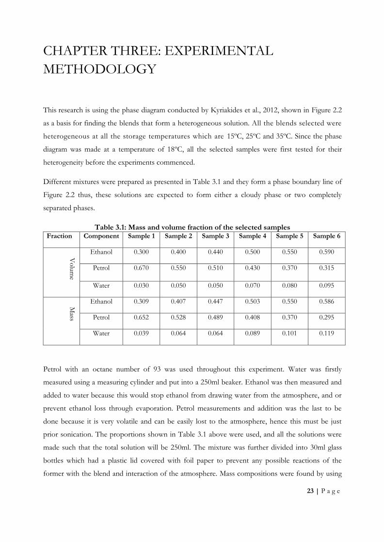
CHAPTER ONE: RESEARCH BACKGROUND ..................................................................................... 1
1.1 Introduction ................................................................................................................................. 1
1.2 Objectives .................................................................................................................................... 2
1.3 Motivation ................................................................................................................................... 2
1.4 Problem statement ....................................................................................................................... 3
CHAPTER TWO: LITERATURE REVIEW .............................................................................................. 4
2.1 Benefits of blending petrol with ethanol ....................................................................................... 4
2.2 Limitations to the use of ethanol .................................................................................................. 4
2.3 Ways in which water can enter into ethanol .................................................................................. 6
2.4 Ternary diagram ........................................................................................................................... 6
2.5 Ways of classifying gasoline .......................................................................................................... 7
2.6 Research done on ethanol blending .............................................................................................. 8
2.7 Sonication .................................................................................................................................. 14
2.8 Physical effects on liquid mixing ................................................................................................ 22
CHAPTER THREE: EXPERIMENTAL METHODOLOGY ................................................................. 23
3. 1 Experimental procedure ............................................................................................................. 24
3. 1.1 Mixing and preparation of samples ..................................................................................... 24
3. 1.2 Determination of chemical composition ............................................................................ 26
3. 1.3 Stability of fuel blends ........................................................................................................ 27
3. 1.4 Characterisation of fuel blends ........................................................................................... 28
3. 2 Data Gathering .......................................................................................................................... 29
CHAPTER FOUR: RESULTS AND DISCUSSION ................................................................................ 30
4. 1 Initial phase separation ............................................................................................................... 30
4. 2 Determination of energy content of the blends .......................................................................... 32

iv | P a g e
4. 3 Sonication process ..................................................................................................................... 33
4. 4 Operating conditions of the sonication process .......................................................................... 35
4.4.1 Temperature profile during blending ...................................................................................... 35
4.4.2 Time for obtaining a homogeneous blend .............................................................................. 38
4.4.3 Initial temperature of the homogeneous blend ....................................................................... 39
4. 5 Storage Analysis ......................................................................................................................... 40
4. 6 Phase diagram comparison ......................................................................................................... 43
CHAPTER FIVE: CONCLUSION AND RECOMMENDATIONS ....................................................... 46
5.1 Conclusion ................................................................................................................................. 46
5.2 Recommendations ..................................................................................................................... 46
References ................................................................................................................................................. 47
Appendix ................................................................................................................................................... 50

1 | P a g e
CHAPTER ONE: RESEARCH BACKGROUND
1.1 Introduction
Ethanol blends are alternative sources of energy in the transport sector in many countries. In the
U.S, most of the gasoline blend is sold as E10, meaning that 10% by volume of the gasoline is
ethanol and the balance being gasoline. However, some of the ethanol is used to make E85
which is mainly used for vehicles with a flexible fuel intake. Countries like Brazil produce ethanol
mainly from sugar cane and they export it to many countries. Currently, in countries like the
U.S.A., ethanol production from wheat and cellulose which includes woodchips and switchgrass
is expected to increase. Globally there is a general increase in the use of blended gasoline with
ethanol. This is mainly because of the environmental awareness of the benefits of bio-fuel and
hence policies have been established that favours their use (Babiuch 2008). A study by Babiuch at
NREL in 2005 shows that when one takes into account the lower mileage impact of ethanol,
ethanol blending reduces the consumption of gasoline by about $0.17 per gallon. They also
concluded that through this, ethanol can be used in the regulation of crude oil prices in the
future when gasoline shortage becomes worst. This is so because ethanol is a very good
substitute of gasoline when compared to diesel. Ethanol is cheaper than gasoline and is one of
the best oxygenates, i.e., it improves the combustion of gasoline, thus it makes it cheaper to sell
blended gasoline. Furthermore, it reduces the import of fossil gasoline but the total comparison
of the two relies more on the prices of the raw materials used for ethanol production and also
the price of crude oil (Babiuch 2008).
The temperature of the environment determines the extent of stability of the different fuel
blends and this will be discussed in detail in the methodology section. In this research, a
thorough investigation of the stability of ethanol blended gasoline will be done at average
temperatures of 15ºC, 25ºC and 35ºC. These petrol:ethanol mixtures were blended using a
sonicator. This will contribute more on the effectiveness of using different gasoline blends
with respect to the different seasons according to the geographical conditions.
Besides ethanol, other sustainable fuel blends have been investigated before, this includes TEL,
tetra ethyl lead, which helped with anti-knocking but had some health effects. Methyl tert-butyl
ether (MTBE) was also used as an oxygenate but it had some negative effects on underground
water (French et al., 2005).
2 | P a g e
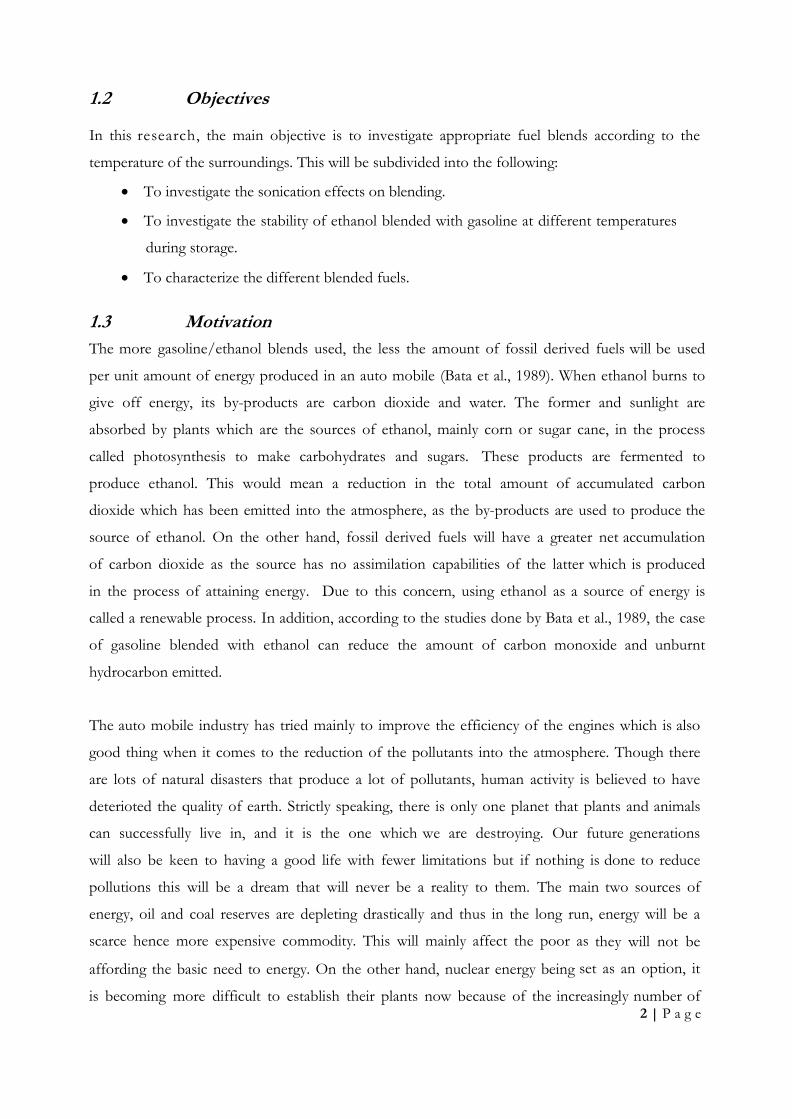
1.2 Objectives
In this research, the main objective is to investigate appropriate fuel blends according to the
temperature of the surroundings. This will be subdivided into the following:
To investigate the sonication effects on blending.
To investigate the stability of ethanol blended with gasoline at different temperatures
during storage.
To characterize the different blended fuels.
1.3 Motivation
The more gasoline/ethanol blends used, the less the amount of fossil derived fuels will be used
per unit amount of energy produced in an auto mobile (Bata et al., 1989). When ethanol burns to
give off energy, its by-products are carbon dioxide and water. The former and sunlight are
absorbed by plants which are the sources of ethanol, mainly corn or sugar cane, in the process
called photosynthesis to make carbohydrates and sugars. These products are fermented to
produce ethanol. This would mean a reduction in the total amount of accumulated carbon
dioxide which has been emitted into the atmosphere, as the by-products are used to produce the
source of ethanol. On the other hand, fossil derived fuels will have a greater net accumulation
of carbon dioxide as the source has no assimilation capabilities of the latter which is produced
in the process of attaining energy. Due to this concern, using ethanol as a source of energy is
called a renewable process. In addition, according to the studies done by Bata et al., 1989, the case
of gasoline blended with ethanol can reduce the amount of carbon monoxide and unburnt
hydrocarbon emitted.
The auto mobile industry has tried mainly to improve the efficiency of the engines which is also
good thing when it comes to the reduction of the pollutants into the atmosphere. Though there
are lots of natural disasters that produce a lot of pollutants, human activity is believed to have
deterioted the quality of earth. Strictly speaking, there is only one planet that plants and animals
can successfully live in, and it is the one which we are destroying. Our future generations
will also be keen to having a good life with fewer limitations but if nothing is done to reduce
pollutions this will be a dream that will never be a reality to them. The main two sources of
energy, oil and coal reserves are depleting drastically and thus in the long run, energy will be a
scarce hence more expensive commodity. This will mainly affect the poor as they will not be
affording the basic need to energy. On the other hand, nuclear energy being set as an option, it
is becoming more difficult to establish their plants now because of the increasingly number of

3 | P a g e
natural disasters some of which are due to the global climate change.
Ethanol blending with gasoline is a good consideration when it comes to finding an
alternative source of energy. It is an opportunity for other countries to develop their domestic
ethanol industries with a good example being Brazil which is a main ethanol producer and
exporter. Furthermore, this will also increase employment opportunities to the local people of the
ethanol producing country. The same can be practiced here in Southern Africa, as land and rain
is not a major concern in most of its parts. Southern Africa does not have a lot of water
reserves to support too much hydroelectricity. In Zimbabwe, they have already introduced
mandatory E10 blending and they are looking at having more volumes of ethanol in petrol.
1.4 Problem statement
The problem with ethanol blending is the instability of the blend when exposed to certain
amount of water as this might lead to phase separation. This results to the formation of two
phases in the blend which is not suitable for use as an energy source.
4 | P a g e
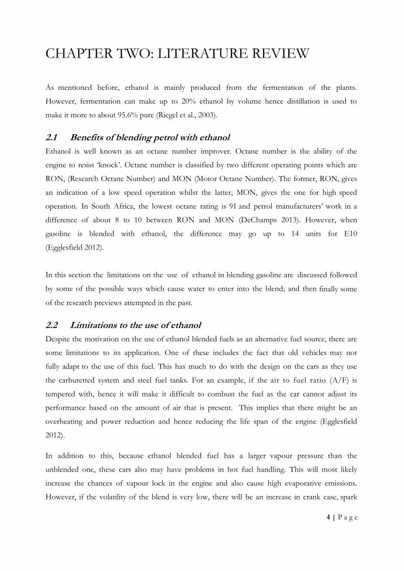
CHAPTER TWO: LITERATURE REVIEW
As mentioned before, ethanol is mainly produced from the fermentation of the plants.
However, fermentation can make up to 20% ethanol by volume hence distillation is used to
make it more to about 95.6% pure (Riegel et al., 2003).
2.1 Benefits of blending petrol with ethanol
Ethanol is well known as an octane number improver. Octane number is the ability of the
engine to resist ‘knock’. Octane number is classified by two different operating points which are
RON, (Research Octane Number) and MON (Motor Octane Number). The former, RON, gives
an indication of a low speed operation whilst the latter, MON, gives the one for high speed
operation. In South Africa, the lowest octane rating is 91 and petrol manufacturers’ work in a
difference of about 8 to 10 between RON and MON (DeChamps 2013). However, when
gasoline is blended with ethanol, the difference may go up to 14 units for E10
(Egglesfield 2012).
In this section the limitations on the use of ethanol in blending gasoline are discussed followed
by some of the possible ways which cause water to enter into the blend; and then finally some
of the research previews attempted in the past.
2.2 Limitations to the use of ethanol
Despite the motivation on the use of ethanol blended fuels as an alternative fuel source, there are
some limitations to its application. One of these includes the fact that old vehicles may not
fully adapt to the use of this fuel. This has much to do with the design on the cars as they use
the carburetted system and steel fuel tanks. For an example, if the air to fuel ratio (A/F) is
tempered with, hence it will make it difficult to combust the fuel as the car cannot adjust its
performance based on the amount of air that is present. This implies that there might be an
overheating and power reduction and hence reducing the life span of the engine (Egglesfield
2012).
In addition to this, because ethanol blended fuel has a larger vapour pressure than the
unblended one, these cars also may have problems in hot fuel handling. This will most likely
increase the chances of vapour lock in the engine and also cause high evaporative emissions.
However, if the volatility of the blend is very low, there will be an increase in crank case, spark

5 | P a g e
plug and combustion chamber deposits. The volatility problem can also be aligned with the high
heat of vaporisation of ethanol which is a problem in cold weather conditions and will result
in the car having some problems with start-up. The volatility problem is encountered by
making the gasoline more volatile in winter and vice versa for summer (Reynolds 2002).
Most fuel tanks are not designed to handle much water, but since ethanol has a high affinity to
water, corrosion of the tank may result. A corroded tank can either increase the chances of holes
being formed or to the blocking of the fuel supply. It is also debated that the use of ethanol
on old model cars may result in early deterioration of components like delivery pipes, injector
seals, regulator and fuel pipes (Egglesfield 2012).
Furthermore, in a two stroke engine, it has been illustrated by Korotney et al., 1995 that if
there is phase separation, ethanol and water phase will compete for running into the engine
with the other gasoline phase and this will result in less lubrication hence damaging the
engine. In the four stroke engines, the combustion of the water phase may result in a creation of a
leaner fuel combustion ratio, i.e., higher A/F greater than normal. Combustion of a leaner fuel will
result in a temperature rise, hence reducing the life span of the engine.
In a study by Kyriakides et al., 2012, the use of ethanol has got no significant deteriorating effects
on the engine except for the fuel pump. After a few hundred hours of continuous engine work, it
was observed that the fuel pump with the gasoline ethanol mixture had changed its colour although
there was no significant thin lining of deposits that was observed. They concluded that both
external aluminium and steel internal cases were highly affected by the presence of ethanol.
Akasaka et al., 2005, also confirmed the effects of ethanol on the changing of the colour in
aluminium fuel pump. On the other hand, commercial gasoline fuel did not show any significant
changes on the fuel pump material. Figure 2.1 shows the effects that were observed. They
suggested that the material of the fuel pump has to be changed in order to meet the safety
requirements required in the automobiles.

6 | P a g e
Figure 2.1: Effects of fuel type on the fuel pump materials after a few 100 hours of test
(Kyriakides et al., 2012).
2.3 Ways in which water can enter into ethanol
Water can enter into the tank as a mixed solution with the fuel or in its own phase. If water enters
the fuel through as a mixed solution, there will be a dilution factor of the fuel and this will
decrease the energy value of the fuel per unit volume. However, this has been proven to be of
less significance in pure gasoline. Depending on the humidity of the atmosphere, water which has
a high affinity to ethanol hence water may condense and enter into the blended fuel.
Furthermore, still depending on humidity, water can enter the gasoline phase through the
absorption of air moisture into the fuel. This would mean that blended gasoline must not be
stored for long periods of time in a high humidity area and or might need emptying of the fuel
tank regularly (Egglesfield 2012).
2.4 Ternary diagram
Since water is not soluble in petrol, but ethanol is soluble in these two, a ternary diagram is a great
interpretation of the mixture ratios that form a single phase. In this report, the ethanol gasoline
phase diagram to be used is the one in Figure 2.2 below. This ternary diagram was developed by
Kyriakides et al., 2012 at a temperature of 18ºC. It was developed in terms of the mixture volume
fraction.

7 | P a g e
Figure 2.2: Ternary diagram for commercial gasoline, water and ethanol blend
(Kyriakides et al., 2012).
2.5 Ways of classifying gasoline
Besides the octane number discussed before, there are also some numerous ways of
classifying the fuel according to South African standards. All the gasoline in the country must have
at least an octane number of 91 but products of 93 and 95 are also available in the market.
The Reid vapour pressure, which is the measure of the pressure of the fuel, has to be in a range
of45kPa to 75kPa (Dechamps 2013).
Furthermore, the fuel is also classified according to the distillation graph with Figure 2.3 being an
example of one that is used by South African gasoline manufacturers.

8 | P a g e
Figure 2.3: Distillation curve of gasoline suitable for the market (Reynolds 2002).
If the fuel is very volatile it will be way below the curve and the reverse is true.
2.6 Research done on ethanol blending
A study conducted by Rajan et al., 1982, included the investigation of the miscibility
characteristics of hydrated ethanol and gasoline. This was done in order to find out how much
water can be tolerated by a certain composition of ethanol in a blend. Ethanol is very much
miscible with water and also with the gasoline. It is very difficult to get pure ethanol as it
reaches a pinch point at around 99%, and most of this alcohol will be made from plants hence
their water content will be high. Separation of ethanol from water requires distillation which
requires a lot of energy hence there is a need to find the maximum tolerable water
concentration in order to optimise the blending of gasoline. Blended gasoline phase
separation was used to notify the maximum tolerable amount to the fuel. In order to find the
maximum water concentration tolerable before phase separation, they first made different
concentrations of water ethanol mixtures of a range from 0-30%. They then added unleaded
gasoline until the mixture becomes saturated which means that phase separation would occur by
any amount of gasoline into the hydrated mixture. However, this was difficult to determine
immediately, hence they left the blended gasoline for at least 6 months. The data was recorded
and they obtained from the miscibility studies is as shown in Figure 2.4.

9 | P a g e
Figure 2.4: Miscibility studies of hydrated ethanol and gasoline (Rajan et al., 1982).
Figure 2.4 shows that ethanol volume percentage in the blend increases with increase in water
composition in ethanol up to about 17% by volume. According to Rajan et al., 1982, this was
due to gasoline being in lower compositions which will make it more soluble. The decrease in the
ethanol content is due to the greater water composition in the non-gasoline phase. Since water
forms stronger hydrogen bonds with ethanol unlike in gasoline where it will only form the weak
Van der Waals forces, it will favour the water phase. His studies were then furthered up to the test
engine combustion with these samples and he concluded that a 6% by volume hydrated ethanol has
the same thermal and power efficiencies as the base gasoline.
French et al., 2005, also studied the blending of ethanol into fuels and pointed out that the
difficulties of the blended product was due to the fact that ethanol forms a non-ideal mixture
with gasoline and hence according to Roult’s law it forms a mixture that forms an azeotrope. He
measured the volatility properties by using the Reid vapour pressure (RVP) which is defined
by ASTM test procedures D-323 or D-5191 of the fuel blended. This was measured at a
temperature of 38ºC in a vessel with a vapour to liquid volume ratio of 4:1. As shown in Figure
2.5, he found out that there was a sharp increase in RVP as alcohol composition was increased
but only up to approximately 4-5% ethanol. Following this was a very gradual decrease at levels
of 4-5% ethanol and more. This means that mixing a non-blended gasoline and E10 will
result in a mixture of a higher RVP indicating the complications associated with blending.

10 | P a g e
Figure 2.5: Effects of ethanol concentration on gasoline RVP (French et al., 2005).
French et al., 2005 also discussed about the gasoline blend phase separation and to him, it was
the most serious problem that is conducted in the blending product storage. In his article,
emphasis was made on not transporting ethanol blended gasoline as this might form two phases. In
general, since ethanol forms stronger hydrogen bonds with water as compared to the Van Der
Waals forces formed with gasoline, when two phases are formed, a significant amount of ethanol
will be in the water phase. If more than one phase is produced, then one has to purge out the
water phase which also contains a lot of ethanol and this is not economical.
Furthermore, some non-negligible amount of hydrocarbons from gasoline will also be in the
water phase due to cosolvency but the amount is depended on the concentration of aqueous
ethanol. However, it is more desirable to add ethanol at the gasoline terminals. French et al.,
2005 also carried out a LLE (liquid-liquid equilibrium) on the blend. Water and ethanol are fully
miscible but the former is not miscible with hydrocarbon, hence the system is classified as a Type
1. Since gasoline is a mixture of different organic compounds, a representative molecule was
selected to be trimethylpentane. Temperature also plays an important role in ethanol
distribution. According to French et al., 2005, findings, as temperature decreases, the two phase
region increases hence the water tolerance also decreases. The ternary diagram below shows
how ethanol was distributed between the two phases.

11 | P a g e
Figure 2.6: Ternary diagram of the distribution of ethanol in water and gasoline at different
temperatures (French et al., 2005).
Figure 2 . 6 shows that water tolerance is not linear with ethanol content thus, phase
separation can be caused by dilution of a blend that is near saturation.
Some studies have also been done on finding some appropriate cosolvents. According to
Keller et al 1971, C3-C8 aliphatic alcohols were proved to be good cosolvents but 1-hexanol was
reported to be the best (Cox 1979). However, the problem with these alcohols is that they are
mainly derived from petroleum sources hence they are not renewable sources. The component
causing a suppressing effect on the phase separation in the eucalyptus oil was studied by
Barton A.F.M., 1988. They concluded that the amount of water that can be tolerated by
gasoline depends on the temperature, ethanol concentration, gasoline concentration and
the concentration of the cosolvent present. They discovered that in the oil components like α-
pinene, α-phellandrene and limonene, which are terpene hydrocarbons, mostly have negative
effects on the stability of blended gasoline. However, molecules in the eucalyptus oil which had
the aromatic ring, like p-cymene, had a slight positive effect on the blending of gasoline with
ethanol. Keller et al 1971, findings showed that the most effective compounds were piperitone,
citronellal and 1,8-cineole but their availability and high costs of production are the main
limitations to their large scale implementation. Though citronellal is slightly better than 1,8-
cineole, it is not preferable to use because it is an aldehyde thus it has the possibility of being
oxidised into an acid hence making it corrosive to the engine. Therefore, according to his
research, 1,8-cineole was found to be the most effective because it is readily available from many
eucalyptus species.

12 | P a g e
Karaosmanoglu et al., 1996, used fusel oil (FO) which was fractionally distilled to make a higher
boiling fraction which was above 120ºC and 75% v/v of FO. They abbreviated it as FOF and it
contained only 0.1% v/v water. FO which was obtained as a by-product in the ethanol
production, had a high amount of water, 8.6% v/v, and by distillation, water was reduced.
Besides this, the chemical composition of FO and FOF contains some fermentation amyl
alcohols. Karaosmanoglu et al., 1996 used different gasoline fuels which were unleaded and they
have got it from Turkish Petroleum Refineries. Karaosmanoglu et al., 1996 concluded that
increasing the amount of fusel oil fraction in gasoline blending with ethanol increases water
tolerance level and the phase separation temperature (PST) decreases. In addition to this, they
also discovered that the higher the aromatic content the lower the phase separation temperature,
hence the chemical composition of the gasoline is very important when blending with ethanol. In
the presence of FOF, environmental temperature was also concluded to be a very important
factor in blending gasoline. The higher the temperature, the more the water tolerance level is.
In other words, the lower the amount of blending agent needed for a stable blend to be
produced. Karaosmanoglu et al., 1996 found that with the use of FOF, gasoline blends with
gasoline rich in aromatics and containing 0.1% FOF can prevent phase separation even in climate
conditions of -10ºC. This shows that by product in ethanol production can be effectively used to
solve the phase separation problem which is the same function as other cosolvents. Figure 2.7
shows the different water tolerances of the various blends.
Figure 2.7: Water tolerance as a function of ethanol in a gasoline fuel with an RVP of
59.9kPa (Karaosmanoglu et al., 1996).
In the publication by Lange et al., 1994, they made a remark on the ability of how oxygenates and
aromatics can reduce the amount of hydrocarbons, CO and NOx emissions in an
automobile exhaust. However, ethanol has a lower potential heat energy content as compared to

13 | P a g e
gasoline, therefore the more the amount of the former in the blend, the lower the heat energy
content the blend will have (Hsieh et al., 2002). In addition to this, increasing ethanol content
also increases the Reid vapour pressure and it also changes both the distillation curve and
compositions, therefore the blended gasoline mixture will evaporate easily (Hsieh et al.,
2002). In order to counteract this, other methods are employed in order to reduce the
evaporative emissions from the gasoline blend. In addition to this ethanol blended gasoline
fuels emit a significant amount of unburned ethanol, acetaldehyde emissions and also acetic acid
emissions (Poulopoulos et al., 2001; Zervas et al., 2002).
He et al., 2002 shows that the addition of ethanol increases the gasoline octane rating. Three
samples were made, the one that had no blend, E10 and E30. The initial and end boiling point
temperatures of the three samples, 10%, 50% and 90% mixtures by volume, were measured.
However, the distillation temperature of the blends increases when compared to the non-
blended one except for the initial boiling point which increases. In addition to this, they used an
addition to find out the effects of blending of the emissions of the fuel. At the operating
conditions, CO and NOx emissions were slightly reduced in the blended fuels but total
hydrocarbon emissions, THC, out of the engine can be greatly reduced by blending.
However, at idling, E10 has little decreasing effects on the amount of CO, THC and NOx
emissions out of the engine, but some drastic emission reduction are observed with E30. One of
the other conclusions they made was that ethanol blended fuels decrease the brake specific energy
consumption, hence ethanol improves the engine combustion efficiency. One of the problems
with ethanol blending is that as ethanol composition increases, the amount of unburned
ethanol out of the engine also increases. Pt/Rh three way catalysts cannot effectively convert
unburned ethanol to carbon dioxide but it is excellent with acetaldehyde emissions (He et al.,
2002).
Rang et al., 1999, conducted a study whereby amongst various stabilities of the blending of
petroleum, they also investigated the effects of water content on the stability of the fuel.
Although they admitted that water was not favourable for it to be in the petrol, they also made a
remark on it being a helper in the combustion of gasoline in the engine. This is so because it helps
in the powering of the gasoline engines. They also demonstrated that very low water content
can improve or reduce the concentration of toxic compounds such as CO and NOx. Magnin et
al., 2000 also notified that water in gasoline helps in the powering of the spark ignition
engines. However, water reduces the calorific value of gasoline. In order to increase the water

14 | P a g e
stability in the gasoline, fatty acids or ethanolamines can be used which can make the blend to
have about 36 to 40% by volume (Wenzel D. 1999). In addition to this, Bertha A. 2000 also
made a claim that it is possible to use C5-C10 carboxylic amides as additives which will enable the
hydrocarbon fuel with a water content of 10-40% by volume. However, the stabilizer has to be
in high concentrations and in this article no specifications showing the effects of the acid on
the engine were shown. The probability is very high that the engine would corrode easily due to
the corrosiveness of the acid.
2.7 Sonication
The initial work of cavitation can include Lord Rayleigh theory on the collapse of a single spherical
bubble under a static pressure (Lord Rayleigh, et al, 1917). This was then followed by combining
this with the explosive growth phase of a small bubble which resulted in the characterization of a
certain cavitation due to small bubbles in a strong sound field. It was explained that the bubble
growth phase is approximately isothermal and the collapse phase being adiabatic. This makes the
bubble serving to concentrate the acoustic energy (Blake et al., 1949.). Flynn then distinguished
between transient and stable cavitation as the latter is less energetic. The work was mainly focussed
on oscillations of individual bubbles in acoustic fields with intense pressure field (Flynn 1964). In
this transient collapse, a range of potential local effects, which includes gas shocks (Vaughan et al.,
1986) and gaseous hot spot (Noltingk et al., 1950; Suslick et al., 1986) is generated from energy
focussed within the bubble.
These effects can amount to the formation of free radicals together with other reactive chemical
species within the bubble gas. Sonoluminescene, which is the production of light by passing sound
waves in a solution, is generated due to this subsequent reaction. These effects are mainly due to
inertial cavitation, which happens in high energies of collapse obtained when inertial forces
dominate the collapse rather than on the temporal characteristics (Walton et al., 1984).
T.G. Leighton then studied the indirect action of sonochemistry due to the populations of the
bubble, not a single one only. In low amplitude acoustic field, the resonance frequency is inversely
related to the bubble radius (Minnaert 1933). The bubbles with diameters close to the resonant
acoustic frequency dominate the effects of the field. In a case where there is a steady increase or
decrease in the equilibrium radius, Ro, there are two explanations to it, the area effect or a shell
effect. The former arises due to the relationship between the mass flux and the area of the bubble
wall. If the radius is less than Ro, the gas contained will be at a greater pressure than the normal

15 | P a g e
equilibrium value thus the gas diffuses from the bubble to the liquid and the reverse is true. On the
other hand, the shell effect results when the gas diffusion rate is proportional to the concentration
gradient of the dissolved gas (Leighton et al., 1994).
According to Hielscher 2005, when a sonicator is used in liquids, there is a continuous formation of
alternating high and low pressure cycles and this depends on the frequency of the sound waves.
Like in any other form of medium, sound travels in liquids by stretching the molecular spacing,
thus making other sections of the medium to be compressed. This will give rise to the variation of
the average distance between the molecules, and hence the difference in pressure distribution
across the liquid medium. The compressed parts with the minimum intermolecular distance are
high pressure ones, whilst the opposite is true (Santos et al., 2009). The high pressure cycle is due
to compression and the low pressure is due to rarefaction. Since the temperature at which a liquid
boils or evaporates is proportional to the surrounding pressure, the low pressure cycles makes it
easy for vapours to form. This leads to the formation of small vacuum bubbles in the liquid and the
gas will continue to absorb energy and thus increasing the volume of these small bubbles. A point
is reached whereby it will not be possible for more energy to absorb and this is where they collapse.
It mainly happens in the high pressure cycles, where by the pressure inside the bubble will be too
low to keep it in the gaseous phase. The collapse can produce high temperatures, up to 5000K,
high pressures of, up to 1000atm, very massive cooling or heating rates, greater than 109 K/sec, and
some jet streams are also formed in the liquid. The process of bubble destruction is very violent
and it is called cavitation (Suslick 1998).
However, a note must be put on the different types of cavitation bubbles that can be formed. The
cavitation bubbles formed can behave as stable cavitation, which is the bubbles formed at very low
intensities such as 1-3W/cm, and for many acoustic cycles will oscillate about some equilibrium
size or transient cavitation. The other form is called transient cavitation, whereby an intensity of
greater than 10 W/cm is used and these ones expand through limited acoustic cycles to about a
radius of at least twice their initial size before they collapse violently on compression. Transient
cavitation is the one that shall be of main use throughout this report. Figure 2.8 shows the
illustration of the difference between these two cavitation bubbles (Santos et al., 2009).

16 | P a g e
Figure 2.8: Creation of stable cavitation bubbles (Hielscher 2005).
Where a is the displacement (x) graph
b is the transient bubbles
c is stable cavitation
d is pressure (P) graph
Not all of the sound energy is absorbed by the liquid particles. Apart from cavitations, some of the
sound energy is transformed to friction, turbulences and waves. Amongst so many factors, the rate
at which the energy is absorbed by the molecules is depended on the magnitude of the pressure
difference created. The higher it is, the greater the probability of the creation of the vacuum
bubbles. In the sonicator, the higher the intensity, the more the energy transferred for the
cavitation formations. The intensity is directly proportional to the amplitude of the sonicator, thus
higher amplitudes results in a more effective formation of cavitations (Hielscher, 2005).
Emulsifications are formed when a liquid which forms two immiscible phases is sonicated resulting
in an evenly distributed phase. Furthermore, the cavitations formed will implode on the two phase
boundary resulting in shock waves being released. This will lead to the formation of very stable
emulsions which will result in a homogeneous solution being formed. This is a very effective way
of mixing since they require less surfactants if ever they are needed as compared to the solution
mixed mechanically by devices such as propellers. This is because the former generally produces
emulsions with less diameter as compared to the latter. They are mainly used in the textile,
cosmetic, pharmaceutical, food and petrochemical industries (Wu et al., 2007).
With time being made a constant factor, there is an increase in cavitation yield with increasing
sound intensity (Feng et al., 1996). However, this relationship will not be linear and it approaches a

17 | P a g e
maximum followed by a decrease in yield with increasing sound intensity. On the other hand, the
cavitation yield increases almost linearly with increasing time (Xu et al., 1992). In a low frequency
range, sonochemical yields decrease with increasing sound frequency. However, in the range of 20-
60 kHz, the yield increases with increasing frequency and this is explained by the influence of the
resonant frequency corresponding to the maximum probability distribution of the nuclear bubble
size. For this reason, the sonication frequency should be as near as possible to the resonant
frequency corresponding to the maximum probability of maximum probability distribution of the
nuclear bubble size (Huang et al., 1995).
Some of the things to focus on with the sonicator are the combination of two or more frequencies
applied to the solution. This has been reported to have significantly increased the cavitation yield.
The interpretation includes the idea that the combination of two or more frequencies would
significantly increase the solution disturbances and thus surface continuity can be easily broken
down by this combination of frequencies as compared to a single frequency. An increase in the
disturbance can also enhance the bubble sound interaction and also the bubble-bubble interaction
through forces which can lead to the fragmentation of the bubble. Mass transfer properties are also
increased by having a combination of different frequencies. Bubbles from a low frequency have the
possibility of providing new cavitation nuclei for its frequency and also others (Zhao et al., 2005).
Mixing with ultrasound does not only limit to phase separations, but also has been concluded to
have some great effects on the mass transfer effects in chemical reactions. Examples of these
include the formation of biodiesel from methanol and soya bean oil. It is explained that the
ultrasound helps in the formation of acoustic cavitation which results in the formation of small
droplets and hence a larger interfacial areas in the liquid-liquid interfaces. They concluded that on a
semi batch reactor, it is not the power per unit mass but dissipated power that affects the reaction
rates (Monnier et al., 1999).
In a study of droplets formed by an impeller, done by Wu et al., 2007, the correlation between the
impeller dimensions and the power it releases into the solution is as follows
⁄⁄ 1
Where

18 | P a g e
Where P is power consumption
N is the speed of the impeller d is the diameter of the impeller C is a constant
is the density
is viscosity g is gravitational acceleration
If there are two immiscible liquids, the critical agitator speed, is the speed at which the solution is
mixed to become a homogeneous solution. Above the impeller critical agitator speed, the mean
diameter decreases with increase in energy input to the solution. The droplet sizes then reaches a
steady state value because of the equilibrium reached between the breakage and coalescence
process. However, the mean droplet sizes changes with the impeller speed, as lower speeds yield
larger drop sizes. On the other hand, if ultrasonic agitation is used, the droplet sizes are much
smaller as compared to the ones produced by an impeller as shown in Figure 2.9 (Wu et al., 2007).
Figure 2.9: Comparison of differential droplet distributions for impeller and ultrasonic agitation with input energy equal to 10.8MJ/m3 (Wu et al., 2007).
At lower energies such as 10.8x10⁶ J/m3, there is a wide range of mean size droplets on the
ultrasonicator as compared to the impeller. If larger input energies are used, greater than 50x106
J/m3, droplets with lower mean diameters can be achieved which will be at least 3 times smaller
than the impeller speed of 1000rpm. Though the input power may vary, the shape of the droplet
size distribution is the same, but the greater the intensity, the lower the mean diameter (Wu et al.,
2007). However, as the intensity increases, the mean size density between the intensities drops as
shown in Table 2.1 below.

19 | P a g e
Table 2.1: Relationship between sonicator intensity and droplet size (Wu et al., 2007).
Energy intensity (W)
Average droplet size (nm)
30 156
50 148
70 146
This shows that increasing the intensity above 70W would result in a very small change in the
droplet mean size since there is a very small change from 50W to 70W. Ultrasound has got a lower
mean diameter as compared to the impeller because the former produces pressure waves which
alternately compress and stretch the molecular spacing of the liquid which results in the generation
and collapse of gas and vapour bubbles. This process enables the breakage of larger droplets into
small ones. When comparing to ultrasound, the impeller relies on the generation of turbulent shear
flows which then results in the making of slightly larger droplets. They concluded that the
ultrasonication mixing can produce up to as much as six times that of the conventional agitation
system (Wu et al., 2007).
Acoustic energy has been widely used for emulsification process which is the formation of tiny
droplets in a continuous phase, thus making the mixture a homogeneous solution. This only occurs
when the cavitation threshold, the least pressure to be applied in order to form cavitations, has
been exceeded. Sound is used as a source of energy which makes it possible for a new interface to
be formed (Wood et al., 1927). If the intensity is greater than the mixture’s cavitation threshold,
there is a limiting concentration of emulsion which increases as the intensity if the ultrasound
increases (Neduzhii, 1961). The limit is due to the equilibrium established between the
emulsification and coagulation process (Bondy et al., 1936). Furthermore, the lesser the viscosity of
the solution, the less difficult it becomes to emulsify, and the easier it is to form a homogeneous
solution (Lorimer et al., 1987). According to, Mujumdar et al., 1997, the emulsion quality can be
affected by the position and the phase at which the source of ultrasound in the solution is placed.
When sonicating oil and water mixtures in a period of less than 60 minutes, there is no change in
the chemical reactions in the solutions (Shashank et al., 2007). They showed that with a constant
power output of the ultrasound that was being introduced, the temperature increased and this made
it possible to decrease the interfacial tension and the viscosity, hence increasing the concentration
of the dispersed component. Furthermore, at constant irradiation time, the fraction of the
dispersed volume increases with increase in irradiation power and this was due to the increased

20 | P a g e
amplitude of the interfacial instability, hence increasing the liquid threads break up, thus improving
the hold-up of the dispersed phase. This in turn increases the number of droplets formed thus
increasing cavitation and collapse intensity. They also studied the effects that constitutes to the
droplet size. At constant power, the droplet size was observed to decrease gradually with increasing
time. It is the increase in temperature that enables the vapour pressure to be attained easily, and
thus increasing the number of nuclei for cavitation, which in turn increases the breakage of the
large droplets. The same relationship exists when power is increased with time being a constant
(Shashank et al., 2007).
In a study of the effects of emulsification for the removal of dyes, Djenouha et al., 2008, came up
with Figures 2.10 and 2.11. As explained earlier, the increase in power increases the emulsion
breakage. This is because at low power, the field created has inadequate quantum energy needed to
nucleate the large dispersed droplets. However, as the ultrasonicator power of the system under
consideration increases to a value above 25W, there is a drastic change in the breakage fraction.
This is due to the process of coagulation, coalescence, which will be more dominant as compared
to the emulsification process. Thus the equilibrium will shift at very large power inputs. On the
other hand, time also follows the same trend and the explanation is the same.
Figure 2.10: Variation of phase breakage with increasing ultrasonic power at constant time
(Djenouha et al., 2008).

21 | P a g e
Figure 2.11: Variation of phase breakage with increasing ultrasonic power at constant
power (Djenouha et al., 2008).
Drop size stability and distribution was also studied by Abismaı¨l et al., 1999, where oil water
emulsions were produced either by agitation or ultrasound in the presence of a surfactant,
polyethoxylated (20EO) sorbitan monostearate. An emulsion described as “a heterogeneous
system, consisting of at least one immiscible, liquid intimately dispersed in another in the form of
droplets, whose diameters, in general, exceed 0.1 mm” (Becher P., 1965). He also added that such
systems are unstable and they can be altered by the addition of finely divided solids which will act
as surface-active agents.
Generally, for emulsifications to occur, energy must be supplied to produce some partially stable
mixtures. When the surface tension decreases resulting in the formation of emulsified solution, the
surface free energy, ΔG, is also reduced, as shown by the following equation
2
Where γ is the interfacial tension A is the surface area
It is also assumed that the communition of larger droplets into the smaller ones involves additional
shear forces resulting in the viscous resistance absorbing energy during sonication or absorption.
The temperature will rise as the extra energy is dissipated as heat (Friberg et al., 1993). High
frequency vibrations allow the interfacial waves to be unstable, hence forming large droplets which
are then reduced to smaller components (Li et al., 1978). Furthermore, Abismaı¨l et al., 1999,
discussed about the two different types of emulsification that can occur. The first one is the
reversible one, which involves particle aggregation and migration, whilst the irreversible one with
particle size modification. The former’s flocculation of droplets is determined by densities which

22 | P a g e
results in sedimentation or creaming, and the latter forms larger drops through Ostwald ripening
and coalescence, thus forming less stable emulsifications and resulting in phase separation. It is also
suggested that the electrostatic or steric repulsion between droplets, for an example surfactants, has
the greatest effect on emulsions. In this study, at 20kHz, they also found out that using the
sonicator instead of a propeller results in less heat energy being lost, and also smaller average
droplets, d32, being as small as 0.3µm.
2.8 Physical effects on liquid mixing
According to Acree W. Jr. 1984, when two substances are mixed, the total volume of the resultant
mixture is not the same as the simple addition of the individual volumes. This is due to the fact that
the solution is real and not ideal. There is an interaction between the bonds which makes the
volumes not add up. Furthermore, when a real solution is formed, the true volume is given by the
following equation
3
Where X is the fractional sum of partial molar volume and given by the following equation
⁄ 4
Where is the number of moles of component .
23 | P a g e
CHAPTER THREE: EXPERIMENTAL
METHODOLOGY
This research is using the phase diagram conducted by Kyriakides et al., 2012, shown in Figure 2.2
as a basis for finding the blends that form a heterogeneous solution. All the blends selected were
heterogeneous at all the storage temperatures which are 15ºC, 25ºC and 35ºC. Since the phase
diagram was made at a temperature of 18ºC, all the selected samples were first tested for their
heterogeneity before the experiments commenced.
Different mixtures were prepared as presented in Table 3.1 and they form a phase boundary line of
Figure 2.2 thus, these solutions are expected to form either a cloudy phase or two completely
separated phases.
Table 3.1: Mass and volume fraction of the selected samples
Fraction Component Sample 1 Sample 2 Sample 3 Sample 4 Sample 5 Sample 6
Vo
lum
e
Ethanol 0.300 0.400 0.440 0.500 0.550 0.590
Petrol 0.670 0.550 0.510 0.430 0.370 0.315
Water 0.030 0.050 0.050 0.070 0.080 0.095
Mass
Ethanol 0.309 0.407 0.447 0.503 0.550 0.586
Petrol 0.652 0.528 0.489 0.408 0.370 0.295
Water 0.039 0.064 0.064 0.089 0.101 0.119
Petrol with an octane number of 93 was used throughout this experiment. Water was firstly
measured using a measuring cylinder and put into a 250ml beaker. Ethanol was then measured and
added to water because this would stop ethanol from drawing water from the atmosphere, and or
prevent ethanol loss through evaporation. Petrol measurements and addition was the last to be
done because it is very volatile and can be easily lost to the atmosphere, hence this must be just
prior sonication. The proportions shown in Table 3.1 above were used, and all the solutions were
made such that the total solution will be 250ml. The mixture was further divided into 30ml glass
bottles which had a plastic lid covered with foil paper to prevent any possible reactions of the
former with the blend and interaction of the atmosphere. Mass compositions were found by using

24 | P a g e
the densities of the individual components. Since petrol is not a single component and has got
various components, the one that was used is 744.7kg/L, ethanol density is 789.3kg/L and that for
water is 1000kg/L.
3. 1 Experimental procedure
The following is an experimental guideline on how the blends were investigated in order to meet
the objectives. Figure 3.1 is a flow chart which shows the overall experimental procedure.
Figure 3.1: Flow chart of the overall experimental procedure
The experiment commenced with the mixing of petrol, water and ethanol in the proportions
respective to the sample being made. The composition of the resultant solution was analyzed
followed by storage at different temperatures. In storage, the sample either maintained a
homogeneous phase, that is, maintain its stability, or formed a heterogeneous solution. If the latter
was formed, the separate phases were analyzed for their different compositions, hence the return loop
shown in figure 3.1.
In order to investigate various blends which are appropriate at different temperatures, this
project first determined the blending effects of the sonicator, chemical composition, and lastly
stability of the blends, that is, the ability to maintain a single phase during their storage.
3. 1.1 Mixing and preparation of samples
In order to mix the blends, a sonicator was used. This device produces sound waves which help in
the mixing of the blends. Figure 3.2 shows the simple illustration of how the equipment was used.

25 | P a g e
Figure 3.2: Sonicator mixing fuel blends
Various sonicator conditions were analyzed. For each of the set sample, concentration of ethanol
was measured before sonication so as to determine the relationship between the water content and
the distribution of ethanol. It was also necessary to determine the effects of the sonicator even in
those samples that will produce two phases after storage. This would give an idea on whether the
ultrasonicator had permanent effects on ethanol distribution even when there is phase separation.
This would help in determining whether it is possible to have a fuel composition with more ethanol
in the petrol phase than it is when normal stirring is done.
Furthermore, it was also of great importance to find the effects of the sonicator parameters on the
blending process. The parameter that was considered is the time for sonication and also the
amplitude of the sonicator. There are two values that were selected for this study, 20% and 40% of
the full sonicator amplitude. Other parameters that can be changed include the number of cycles
produced per unit time, but in the experiments, this was put to a constant value of 1.
The formation of a single phase is also dependent on the temperature of the mixture. Hence
temperature was also measured as the sonication process was performed. A mercury thermometer
was used whereby it was stationed at a selected position. The reason for this is fully explained in the
respective results and discussion section.
The samples that were prepared for storage were each sonicated for 10 minutes at a sonicator
amplitude value of 40%. This was to ensure that all the mixtures had the same bases for
comparison, which is energy and the disturbance sourced from the sonicator in this case. The
temperature was measured before and after sonication as well. This enabled the investigation of the
effects of the solution composition on the final temperature. In addition to this, the homogeneity
of the solution after sonication was noted.

26 | P a g e
3. 1.2 Determination of chemical composition
This marks the second stage of the experimental work. An HPLC was used to analyze ethanol and
water concentration of each of the blends. The necessary training was obtained from the
experienced HPLC operators. There are two types of detectors that are found on the machine.
These are refractive index detector (RID) and ultra violet detector (UV detector). RID was used as
a detector since the UV detector was not giving positive results.
In order to calibrate the machine, respective water and ethanol HPLC standard solutions were used
to develop a method which will be used for all the runs to be made. The solvent used was
acetonitrile, and the column with amino acid as the stationary phase was used. These standards
were purchased from ANATECH and SIGMA suppliers. An appropriate method was developed.
This included the setting up of the right parameters on the machine and this can only be
measured its success when the standards show some equally well developed and
distinguishable peaks. Three samples of ethanol standards were prepared and these had their
areas measured using the HPLC. The concentrations selected are supposed to be a good
representative of the range of ethanol concentration to be measured. The standard solutions
were made by first measuring a mass of ethanol using the electronic mass balance and this
has to be diluted by acetonitrile up to 20ml of the solution in order to get the desired
concentrations. This had to be done very quickly because ethanol is ultrapure hence it has a
tendency of drawing in water from the atmosphere since it has a great affinity for it. Table
3.2 shows the amount of measured mass and the diluted final concentrations.
Table 3.2: Mass and desired standard solutions for calibration
Mass (g)
Concentration (g/L)
0 . 8 4 0
1 . 6 8 0
2 . 4 1 2 0
The precautions taken on the HPLC machine included the attention to detail on the limits
that the column can take. Solid particles must never be allowed to enter the solution that
was analyzed as they can block the machine and the column. If the orientation of the
column is incorrect one is bound to have different results as well. The column used was
Eclipse XDB-C18, which has diameter of 4.6mm and a length of 150mm. The particle size
of the adsorbent in the column was 5µmm and had a void volume of 60%. Its working
conditions are shown in the Table 3.3.

27 | P a g e
Table 3.3: Maximum operating conditions of Eclipse XDB-C18
Parameter Maximum Value
Pressure 400 bar
Temperature 60ºC
pH 9
The conditions for the method developed for ethanol concentration measurement are also
shown in Table 3.4.
Table 3.4: Parameters set to measure the concentration of ethanol
Parameter Value
Pressure 29.4 bar
Temperature 35ºC
Flow rate 1ml/min
Injection volume 20µL
Each component has got its own unique retention time in a particular time. It was observed
that the retention time for the selected conditions on the method developed is 1.8 minutes.
A calibration curve was obtained which related the area under the curve to the
concentration of ethanol. Figure 3.3 is the calibration curve which was a straight line and its
equation is shown below.
Figure 3.3: Calibration curve and its equation
All the measured ethanol concentrations were deduced from this equation. Each run was made to
last for 2.3 minutes.
3. 1.3 Stability of fuel blends
Three water baths were used to store the samples and they were regulated at temperatures: 15ºC,
25ºC and 35ºC respectively. Each temperature was resulted by using a thermostat. The samples
were stored in 30ml sample glass bottles and they had plastic lids. Adequate precaution was taken

28 | P a g e
to ensure that each bottle was air and water tight otherwise the experiments will be ruined. After
sonicating, each sample was then put into the respective water bath. In each water bath, there were
5 samples containing the same composition. This was done because once there is a phase
separation and if one draws some sample from both phases, the equilibrium will be shifted hence a
totally different solution will result. The other reason was to make sure that the error is reduced by
making it possible to repeat the same experiment.
Stirring was avoided during storage since it was not one of the parameters to be looked at during
storage. In order to achieve this, a sample stand was designed which made sure that the samples
was very stable whilst they were in storage. This stand was made at the Wits Chemical Engineering
workshop is shown in Figure 3.4.
Figure 3.4: Water bath in use
3. 1.4 Characterisation of fuel blends
The characterization was conducted by determining the energy content of the samples. This
could not be done experimentally but a rough estimate of this was done using the summation of
the energy that can be contained from each component in a liter. Table 3.5 below shows the high
and low energy content of each of the mixture components. In the calculations made, the low
heating value was used. This is because it is very difficult for one to attain the high heating value of
any component, because some of the molecules will escape without being combusted whilst in
some cases it is very difficult to achieve a complete combustion of the mixture.

29 | P a g e
Table 3.5: Energy and density values of pure ethanol and petrol
Ethanol Petrol
Energy kJ/L (High) 29.85 46.54
Energy kJ/L (Low) 23.56 34.66
Density (kg/m3) 789.35 744.7
3. 2 Data Gathering
Ethanol concentration measurement was obtained before and after sonication and storage. During
the sonication process, the final temperature was noted and when amplitudes were being
compared, it was read every minute. After 30 days the phases that had separated were analyzed for
their respective ethanol concentration in both phases. This was done to determine if the sonicator
had made any changes from the previous solution. Furthermore, on day 60, the phase separated
samples had their ethanol concentrations being measured be done on a weekly basis. The results
found were reported and discussed. The ones that did not form two phases made it possible to
justify the use of the sonicator as a ternary diagram modifier.

30 | P a g e
CHAPTER FOUR: RESULTS AND DISCUSSION
The following results were found when comparing the energy content of the sonicated samples to
the ones which were not. In this section no chemical reactions are assumed to have taken place
during any sonication process since it was only done for a short time (Shashank et al., 2007). In
addition to this, no sonoluminescene was observed thus free radicals are also not formed in this
process (Walton et al., 1984).
4. 1 Initial phase separation
Before sonication, there were two phases formed. The top phase is petrol dominant phase whilst
the other phase is the water dominated phase. Figure 4.1 shows the phase separation that occurred
in the samples when they were settled.
Figure 4.1: Mixed sample with complete phase separations
The samples were made so that the separate mixture components adds up to 20ml. Tables A1 and
A2 in the Appendix shows the actual mixed volumes as shown in Figure 4.1. The total resultant
volume differs from one mixture to another. This is due to the fact that the solution is a real not an
ideal one. As described before in literature, section 2.6, the volumes will all not be equal to 20ml
and this is because the non-ideal forces acting on the molecules of the solution makes the resulting
mixture to be greater or lesser than the sum.
The phase separations are due to the intermolecular forces that occur between the molecules of
petrol, ethanol and water. Water can form hydrogen bonds with ethanol, and ethanol can also form
weaker Van der Waals forces with petrol. This leads to ethanol being distributed between the two

31 | P a g e
phases. In all the experiments, water was put first followed by ethanol and then water. Initially
there is a cloudy phase which as shown in Figure 4.2.
Figure 4. 2: Cloudy sample of mixed solution
The time needed for settling into two completely separated phases is different from one sample to
another. This is because a continuous net movement of the molecules will be taking place and time
to reach equilibrium depends on the amount of each component present. Furthermore, ethanol is
not equally distributed through the two phases hence equilibrium is formed in each of the
solutions. Figure 4.3 shows the ratio of ethanol to water concentration and its distribution between
the two phases at a room temperature of 19ºC.
Figure 4.3: Ethanol distribution compared with water composition
The ethanol distribution between the phases in petrol/water blend, decreases as the amount of
water increases implying that the petrol phase becomes leaner in ethanol. Although there is a little
amount of water present in all the samples, which is less than 12% by mass, the phase separations
are inevitable. This also is an indication of how the hydrogen bonds formed between ethanol and
0.000
0.100
0.200
0.300
0.400
0.500
0.02 0.04 0.06 0.08 0.10 0.12
eth
an
ol
in p
etr
ol
ph
ase
(g
/L
) eth
an
ol
in w
ate
r p
hase
(g
/L
)
Mass fraction of water in solution

32 | P a g e
water overshadows the weak Van der Waals forces between ethanol and hydrocarbon molecules.
The points are most likely to follow a linear relationship except for the one marked in a circle at
x=0.064. This point is taken from the inside the cloudy region of Figure 2.2, whilst the other points
represent the phase boundary. It can be deduced that the ethanol distribution has got a different
correlation when comparing the points on the phase diagram and the ones inside the phase
diagram. Furthermore, the more a point is inside the phase diagram, the more ethanol that is in the
petrol phase. This pose an advantage since more ethanol is associated with petrol, however, the
issue of phase separations has to be addressed as it is the major problem.
4. 2 Determination of energy content of the blends
It is also necessary for one to compare the energy content of the phases and the mixed solution.
Energy was calculated using sum of the low energy values of each of the three components, that is,
water, ethanol and petrol. Water has combustion energy of 0 whilst ethanol has a high heating value
of 23.6kJ/L. Petrol has got the highest energy content amongst the three of them and the value is
34.7kJ/L. The samples prepared in Table 3.1 had their energy analysed for the water phase, petrol
phase and the blended homogenous phase. Figure 4.4 shows the results obtained on sample
analysed and the raw data and calculations done are shown in Table A6.
Figure 4.4: Comparison of water and petrol phase energy content
As shown, the energy content of the petrol phase is always greater than that for water phase per
litre of each phase. In addition to this, if the whole solution has to be put into a single phase, it is
also shown that each of the samples will have a lesser energy content per litre of the solution
compared to the litre of the respective petrol phases only. The reason to this is that it has to be
0
5
10
15
20
25
30
35
1 2 3 4 5 6
Ene
rgy
(kJ/
L)
Sample
Petrol phaseWater phaseMixed solution

33 | P a g e
between the energy contents of the two phases since the petrol phase represents the highest energy
value and the water phase represents the lean values. This is because ethanol has a lower heating
value as compared to petrol and also water has no heat energy content in it. Since the goal is go
green, we cannot eliminate ethanol for this cause.
The greater the amounts of ethanol present in the solution the greater the energy of the petrol
phase. The more ethanol concentration is in the mixture, the more of it that will be distributed in
the petrol phase. Though there are higher chances of ethanol hydrogen bonding with water with
increasing ethanol concentration, water can only take a certain amount of ethanol, thus the rest will
be available for Van der Waal bonding with petrol molecules. This explanation is also supported by
the results shown in Figure 4.3. Though the energy contents of each of the mixed phase are lower
than commercial petrol, it is more desirable to use them as compared to using pure petrol because
it is cheaper and more environmentally friendly. The more the concentration of ethanol present in
the mixture, the less the energy it contains, but the more advantageous it becomes in terms of its
price and environment. However, once there is phase separation, it becomes unfriendly to use the
fuel mixture as water is likely to corrode the engine parts as it will be in high concentrations.
4. 3 Sonication process
In order to achieve the goal of forming a homogeneous solution, a sonicator was used to blend the
mixture. The amplitude used was 40%, and it was set to a cycle of 1. Moreover, the sonication time
was put at a constant time of 10 minutes. Figure 4.5 shows a snap shot of a solution which is being
sonicated.
Figure 4.5: Cavitations formed on sonication
Figure 4.5 shows how the homogeneous phase is formed. It is observed that bubbles are formed
which are always moving upwards. These are due to the effect of cavitations. Cavitations as
described before are high energy containing bubbles which release this energy when they burst, lost

34 | P a g e
as sound or heat, but some of the energy is retained in the molecule. The sound energy from the
sonicator is the source of energy for the molecules in the solution which they absorb in order to
complete their transition from liquid to bubbles. Usually, the two phases in the solution disappears
gradually with the of sonication time. For these experiments, the sonicator tip was always
maintained at a distance of 2cm from the bottom, which makes it to be dipped in the water phase.
According to Mujumdar et al., 1997, the phase in which the sonicator is inserted has got some
effects on the time of blending to achieve a single continuous phase.
The molecules which are near the tip receive the energy from the sonicator and this this increases
their kinetic and heat energy. This makes them to have a temperature and velocity which is greater
than that of the other molecules. The more energy containing molecules will then form a gas
bubble which is less dense than the solution thus these particles move upwards. As they do so, they
will bombard with the other molecules in the solution, transferring some to them as well. This way
of energy transfer is called convection. The molecules on the immediate interface will be
bombarded by the gaseous molecules, where the latter lose energy on impacting with the former.
The molecules on the interface gain enough energy to conquer the interfacial forces holding the
molecules at the phase boundary and they move into the water phase. These molecules will enter
into the solution and they will bombard with the other gas bubbles, breaking them and some of the
molecules will even circulate to the bottom. From this, it can be seen that a continuous cycle is
happening, and this carries on till the molecules are all blended into one phase.
In addition to this, on a micro level, the solution which appears to be a single phase, it is actually a
batch of petrol molecules coagulated together to produce emulsion that enter into the water phase
and hence form a single phase solution. This is explained by the formation of emulsifications,
which make it possible for some particles to be able to get into the other phase. As discussed
before in the literature, the sonicator creates high and low pressure cycles which result in the
formation of cavitations. The formation and destruction of cavitations will result in the phase
boundary to be diminished by the shock waves transferred from one point to another.
Furthermore, the particles are made to be in very small diameters due to cavitation. This will make
them to be more soluble in the bulk phase and thus making it look homogeneous. The hydrogen
bonds still exist and so do the Van der Waals forces, but however, they are no longer dominant if
the sonicator is used which may suggest that they are weakened. This means that the interfacial
forces that make hydrogen bonds to be highly dominant are still available. The explanation to this
is that the smaller molecules produced makes it possible for the particles to be bounded between

35 | P a g e
the bonds and they also maintain the necessary energy to overcome the intermolecular forces. The
smaller the particle size, the more homogeneous the solution will be, and this can be explained in
terms of the ability of the emulsified liquid to fit in the intermolecular spaces. It is also of
paramount importance that an emphasis is put on the fact that these emulsifications occur to
molecules in both phases as the dominant interfacial molecules are weakened in both cases.
4. 4 Operating conditions of the sonication process
The sonicator used had got amplitude and number of cycles as variables. The frequency is constant
at 24Hz and the amplitude can be changed in terms of the percentage from 0-100% whilst the cycle
is from 0-1. However, amplitude was the only parameter that was thoroughly investigated whilst
the cycle was maintained at 1.
4.4.1 Temperature profile during blending
It is also necessary to investigate the temperature trends when one is using the sonication. This is
because petrol is made up of very volatile components, hence the more the temperature rises, the
more the volatile components are lost to the surroundings. This temperature rise as explained
before, is due to the energy lost during the sonication process. The trend of temperature was
compared at two different amplitudes which are 20% and 40% to the full sonicator amplitude. The
temperature readings were each taken after every 1 minute and at a single point from 3cm away
from the bottom of the beaker. This was done so because it is believed that the different pressure
cycles can also cause some slight temperature fluctuations from one point to another (Hielscher,
2005). Figure 4.6 shows the change in temperature with time that was observed when sample 1 was
in the process of sonication. Other graphs, Figure A1-A5 in Appendix, show the remaining
comparisons of other samples and the raw data for these is shown in Table A7 and A8 in the
Appendix section.

36 | P a g e
Figure 4.6: Temperature varying with time at distance from the sonicator probe
As time progresses, there is an increase in temperature from one point to another in all the two
amplitudes. However, the gradient is steeper for the scenario where amplitude is 40% as compared
to the 20% one. This shows that as the amplitude increases, the steeper the temperature gradient.
According to Hielscher, 2005, amplitude determines the way the sonotrode surface travels. The
greater the amplitude, the higher the rate of at which pressure lowers and increases at each stroke,
hence it detects the rate at which the cavitations are formed. The more the cavitations formed, the
greater the amount of energy transferred into the solution thus emulsifying or blending the
substance at a quicker rate. In addition to this, the larger the amplitude, the greater the volume
displaced by each sonicator stroke. This solution will thus be producing more rigorous collision in
the solution and hence the heat transfer will increase with increasing amplitude.
In order to compare the temperature changes in the sonication process, Figure 4.7 was plotted for
up to 4 minutes time at a frequency of 20% and the raw data is shown in Appendix as Table A7.
0
5
10
15
20
25
30
35
0 1 2 3 4 5 6 7
Tem
pe
ratu
re
(ºC
)
time (min)
20%
40%

37 | P a g e
Figure 4.7: Comparison of temperature rise with time in different solutions at 20%
amplitude
The data shown above illustrates how each solution has its own unique trend of rate of temperature
increase with time. Sample 1 has the lowest temperature gradient and sample 2 has the highest
temperature gradient. It is also worthy to note that as the mixture is made, the initial temperature is
not the same. This is due to the heat lost by the breaking down and formation of new bonds in the
solution. Hydrogen bonds are formed by ethanol water mixtures, whist pure water and ethanol
hydrogen bonds are also broken. The same happens with the petrol ethanol Van der Vaal forces
formed, whilst the pure petrol ones are broken.
Figure 4.7 also shows that the temperature profile during sonication blending is depended on the
composition. This is because at low pressure cycles, the cavitations formed will be destructed
depending on the vapour and solution compositions. The two compositions affects the equilibrium
position of the vapour thus it determines if it will collapse or not. The more vapour that collapses,
the more the cavitations formed, hence the more the heat released. The difference in the
temperature gradients is due to the composition of the solution and the pressure cycles formed
therein. The amount of energy released to heat energy is depended on the amount of energy that is
put into the system and also lost. Each solution has got different heat capacities to transfer the lost
energy, thus it will also result in the difference in the temperature gradient.
14
16
18
20
22
24
26
28
30
32
34
0 1 2 3 4 5
Tem
pe
ratu
re
(ºC
)
time (min)
sample 1sample 2sample 3sample 4sample 5sample 6

38 | P a g e
4.4.2 Time for obtaining a homogeneous blend
The effect of the amplitude on the formation of a homogenous or blended solution was also
investigated. The phase homogeneity of the solution was checked after every minute. However, this
could not be recorded in a more discreet way since the homogeneous solution can only be
identified visually and by allowing it to settle and to notice if the mixture has still any cloudy
portions. The samples were made and named according to the compositions defined in Table 3.1
and only volume ratios are considered in the sample description. Figure 4.8 shows the time taken
by each solution to reach to a homogenous solution. Some of the solutions never formed a single
phase solution in a space of 6 minutes and these are the solutions with unshaded pattern.
Figure 4.8: Comparison of the time taken to reach a homogeneous solution
The bar chart above compared the minimum time needed to reach a homogenous solution between
the 20% and 40% frequency of the sonicator. Figure 4.8 shows that the higher the amplitude, the
earlier it will take for a homogeneous solution to be formed. It is observed that there are different
times needed for a given solution to reach a homogeneous solution even if the amplitudes are the
same. This is more explained by the difference in the energy needed to overcome the
intermolecular forces. Furthermore, each solution has different viscosity values, thus the energy
needed to form a single phase is different. Figure 4.8 shows that sample 1 (0.30E: 0.67P: 0.03W)
forms a homogenous solution in the 5th minute whilst sample 3 (0.44E: 0.51P: 0.05W) shows
homogeneity in the 3rd minute for both frequencies. According to this set of results, there is less
effects on the amplitude used in this solution. However, a greater possibility is that the fraction at
which the blend is formed differs with frequency, but in this experiment, time was measured after
every minute.
0
1
2
3
4
5
6
1 2 3 4 5 6
tim
e
(min
s)
Sample number
20% frequency40% frequency

39 | P a g e
In sample 2 (0.40E: 0.55P: 0.05W) sample 4 (0.50E: 0.43P: 0.07W) and sample 6 (0.59E: 0.32P:
0.10W), there is a significant decrease in the time to reach homogeneity when a higher frequency is
used. From Figure 4.8, Sample 2 cannot form a homogeneous solution within 6 minutes when
using a frequency of 20%. Sample 4 and 6 homogenise a minute earlier when using the 40%
amplitude as compared to 2 the 20% one of the respective solutions. As explained before, 40%
frequency will provide more rigorous and violent effects in the solution due to the enhanced rate in
the formation of the high and low pressure cycles. The lower the pressure, the easier it becomes for
cavitations to form, and once they are formed, the higher the pressure, the easier it is for them to
collapse. This will make more cavitations to be made at low pressures whilst more vapours
collapsed due to high pressure. According to Shashank et al., 2007, the greater the amplitude, the
more the power introduced into the solution. It also implies that the increased disturbance due to
higher amplitude on the liquid interface will also increase the liquid breakups which improve the
amount of petrol in the water phase. This enables the particles to acquire quickly the amount of
energy necessary to form the emulsifications and hence the homogeneous solution.
Furthermore, as shown in Figure 4.8, sample 5 (0.55E: 0.43P: 0.07W) does not show any
homogeneity for both of the frequencies in the 6 minute interval. This shows that the amplitude
and energy acquired by the solution could not break the interfacial bonds, hence affirming the fact
that the interfacial forces differ with solution composition.
According to Lorimer et al., 1987, the lesser the viscosity, the lesser the amount of time needed to
form a single phase. As shown in Table A9 in the Appendix, ethanol has the highest viscosity
followed by water. It means that the blends made will have different viscosities since they latter is
depended on the compositions available. This might be the cause of differing amounts of
homogeneity time because the compositions are different in all the samples, thus implying different
viscosities. Another explanation could be that as the amplitude increases, the droplet sizes also
decrease. The smaller the particles, the easier it is for the particles to be dispersed into the solution
(Shashank et al., 2007).
4.4.3 Initial temperature of the homogeneous blend
In order to understand more on the sonication effects, there was a comparison that was made
between the changes in ethanol concentrations in both phases at these two different amplitudes of
the sonicator. Figure 4.9 below shows the results that were found and the samples are named as
before according to Table 3.1.

40 | P a g e
Figure 4.9: The temperature achieved when a homogeneous solution is reached
As shown in Figure 4.9, there is less difference between the two temperatures, but it can be
concluded that at the time when the solution reaches homogeneity, the 20% amplitude will be
lesser than the 40%. This is due to the effects the amplitude has on the formation of cavitations
and this has been discussed in detail, (time for obtaining a homogeneous blend). All the
temperatures are below 40ºC, which is important as high temperatures will result in a great loss in
the amount of volatiles. One point to note from this is that the temperature on forming a
homogeneous blend is generally greater with 40% being than 20%. Higher temperatures will
enable the interfacial forces to be weakened and the viscosity is also reduced (Shashank et al.,
2007). Furthermore, the higher the temperature, the easier it is for the solution to form cavitations
at the low pressure cycle points. This shows that temperature is one of the main causes for the
greater rate of emulsification in the solution at 40% amplitude. However, higher temperatures
reached by the 40% amplitude will cause some problems of volatile components being lost.
Moreover, as shown in Figure 4.8, the higher the amplitude, the lesser the time needed to reach
homogeneity, hence a balance must be obtained between reducing the time for sonication and
sonicator amplitude.
4. 5 Storage Analysis
Each of the samples was sonicated for 10 minutes by 40% amplitude and on a full cycle of the
sonicator. The sonicated samples were stored in water baths of different temperatures, which were
15ºC, 25ºC, and 35ºC and left for 60 days. Each of the samples was made to be in five different
storage bottles in each water bath. This was done so in order to investigate the effect of ethanol
concentration distribution between the two phases, if phase separation occurs. Table 4.1 below
0
5
10
15
20
25
30
35
40
1 2 3 4 5 6
Tem
pe
ratu
re
(ºC
)
Sample
20% frequency
40% frequency
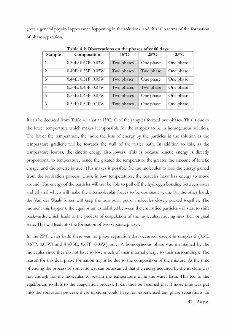
41 | P a g e
gives a general physical appearance happening in the solutions, and this is in terms of the formation
of phase separation.
Table 4.1: Observations on the phases after 60 days
Sample Composition 15ºC 25ºC 35ºC
1 0.30E: 0.67P: 0.03W Two phases One phase One phase
2 0.40E: 0.55P: 0.05W Two phases Two phase One phase
3 0.44E: 0.51P: 0.05W Two phases One phase One phase
4 0.50E: 0.43P: 0.07W Two phases Two phase One phase
5 0.55E: 0.43P: 0.07W Two phases One phase One phase
6 0.59E: 0.32P: 0.10W Two phases One phase One phase
It can be deduced from Table 4.1 that at 15ºC, all of the samples formed two phases. This is due to
the lower temperature which makes it impossible for the samples to be in homogenous solution.
The lower the temperature, the more the loss of energy by the particles in the solution as the
temperature gradient will be towards the wall of the water bath. In addition to this, as the
temperature lowers, the kinetic energy also lowers. This is because kinetic energy is directly
proportional to temperature, hence the greater the temperature the greater the amount of kinetic
energy, and the reverse is true. This makes it possible for the molecules to lose the energy gained
from the sonication process. Thus, in low temperatures, the particles have less energy to move
around. The energy of the particles will not be able to pull off the hydrogen bonding between water
and ethanol which will make the intermolecular forces to be dominant again. On the other hand,
the Van der Waals forces will keep the non polar petrol molecules closely packed together. The
moment this happens, the equilibrium established between the emulsified particles will start to shift
backwards, which leads to the process of coagulation of the molecules, moving into their original
state. This will lead into the formation of two separate phases.
In the 25ºC water bath, there was no phase separation that occurred, except in samples 2 (0.3E:
0.67P: 0.03W) and 4 (0.3E: 0.67P: 0.03W) only. A homogeneous phase was maintained by the
molecules since they do not have to lose much of their internal energy to their surroundings. The
reason for this dual phase formation might be due to the composition of the mixture. At the time
of ending the process of sonication, it can be assumed that the energy acquired by the mixture was
not enough for the molecules to sustain the temperature of in the water bath. This led to the
equilibrium to shift to the coagulation process. It can thus be assumed that if more time was put
into the sonication process, these mixtures could have not experienced any phase separations. In

42 | P a g e
addition to this, according to Figure 4.7, sample 2 has the highest temperature gradient per unit
time. It can be concluded that most of the energy was not absorbed but it was lost as heat energy.
The reason to this is not yet known but it has to do with the physical properties of the solution. A
greater amplitude and longer time can be used in order to have positive results.
A stable phase is established whereby homogeneity is maintained. Though the particles lose some
energy, from the last sonicated temperature to the surrounding one, 25ºC, they still maintain a
constant homogeneous phase. Samples 1 (0.3E: 0.67P: 0.03W), 3 (0.44E: 0.51P: 0.05W) 5 (0.5E:
0.43P: 0.07W) and 6 (0.3E: 0.67P: 0.095W) were observed to have maintained the homogeneity.
This means that the particles maintained a level of energy that could not be kept at 15ºC.
Consequently, this means that the particles in the 15ºC had less internal energy as compared to the
25ºC. This has partly to do with the issue of temperature that was explained before. In addition to
this, sample 2 has been taken inside the phase diagram unlike the other points considered. This
shows that the more one moves away from the ternary boundary, the more difficult it is to emulsify
a solution using a sonicator.
Since all the samples had maintained a homogeneous phase in 35ºC, it shows that less energy had
to be lost in order for the mixtures to maintain the single phase. Furthermore, the blend was also
gaining quite some substantial amount of energy since 35ºC is greater than the ambient
temperature.
On the separated solutions, a comparison was made between the sonicated samples and the stirred
ones. Figure 4.10 shows the comparison of the ethanol equilibrium concentration in the petrol
phase of the simply stirred solution settling in 1 hour and completely separated solution and the
sonicated solutions on days 30 and 60 at 15ºC.
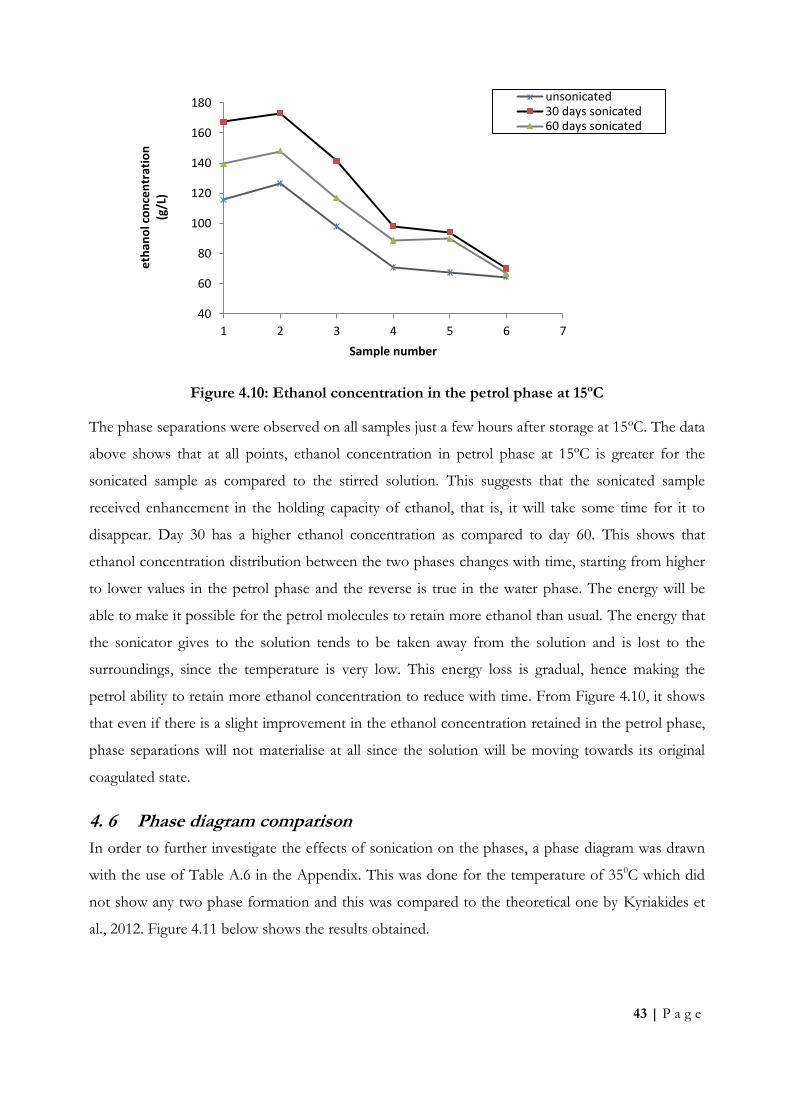
43 | P a g e
Figure 4.10: Ethanol concentration in the petrol phase at 15ºC
The phase separations were observed on all samples just a few hours after storage at 15ºC. The data
above shows that at all points, ethanol concentration in petrol phase at 15ºC is greater for the
sonicated sample as compared to the stirred solution. This suggests that the sonicated sample
received enhancement in the holding capacity of ethanol, that is, it will take some time for it to
disappear. Day 30 has a higher ethanol concentration as compared to day 60. This shows that
ethanol concentration distribution between the two phases changes with time, starting from higher
to lower values in the petrol phase and the reverse is true in the water phase. The energy will be
able to make it possible for the petrol molecules to retain more ethanol than usual. The energy that
the sonicator gives to the solution tends to be taken away from the solution and is lost to the
surroundings, since the temperature is very low. This energy loss is gradual, hence making the
petrol ability to retain more ethanol concentration to reduce with time. From Figure 4.10, it shows
that even if there is a slight improvement in the ethanol concentration retained in the petrol phase,
phase separations will not materialise at all since the solution will be moving towards its original
coagulated state.
4. 6 Phase diagram comparison
In order to further investigate the effects of sonication on the phases, a phase diagram was drawn
with the use of Table A.6 in the Appendix. This was done for the temperature of 350C which did
not show any two phase formation and this was compared to the theoretical one by Kyriakides et
al., 2012. Figure 4.11 below shows the results obtained.
40
60
80
100
120
140
160
180
1 2 3 4 5 6 7
eth
ano
l co
nce
ntr
atio
n
(g/L
)
Sample number
unsonicated30 days sonicated60 days sonicated

44 | P a g e
Figure 4.11: Comparison of the phase diagrams of the unsonicated and sonicated
solutions at 350C
There is a change in the shape of the phase diagram. The cloudy phase, that is the two phase
region, has been reduced, thus extending the homogeneity of the solution. In addition to this, if the
extrapolation of the phase diagram is done on the results obtained through the six solutions
prepared, it can be deduced that the peak of point of the ternary diagram will also move to the
right. This is due to the change in structure that has been imposed in the solution and thus keeping
it as a single phase. The hydrogen bonds have been partially broken whilst the petrol molecules
together with water and ethanol have been internally energized by the ultrasound resulting in a
solution with a different physical structure. The current solution is neither limited by the hydrogen
bonds nor the Van der Waals forces and this is explained by the cavitation formation as discussed
before. As long as these solutions are maintained in a homogenous state, the phase diagram would
have shifted so as to decrease the area of heterogeneous solution whist increasing the one for a
single phase. At low temperatures of storage, the phase diagram did not change because the
0
10
20
30
40
50
60
70
80
90
100
100
90
80
70
60
50
40
30
20
10
0 0.00 10.00 20.00 30.00 40.00 50.00 60.00 70.00 80.00 90.00 100.00
Water
Petrol
Ethanol
None sonicated blend
Sonicated blend

45 | P a g e
solutions formed heterogeneous phases. However, more research has to be done to investigate the
effects of sonication on more solution compositions, so as to find out if the whole ternary diagram
shifts to the left or not.

46 | P a g e
CHAPTER FIVE: CONCLUSION AND
RECOMMENDATIONS
5.1 Conclusion
It is very much possible to alter the ethanol distribution amongst the petrol: water phases using a
sonicator depending on the storage conditions. Cavitations formed by the sonicator will result in
the emulsification of the mixture. Phase separations can be eliminated by a sonicator and but upon
storage, the retention of the single phase formed depends on the temperature. The lower the
temperature, 15ºC, the more difficult it is to maintain a single phase whilst at high temperatures,
35ºC, the solutions are stable enough to maintain a single phase. In winter conditions, none of
these mixture ratios should be used if the sonication process is done under these conditions as
phase separations may be inevitable. However, in very high temperature climates, all the samples
may be used under the sonicator conditions. Thus, the higher the temperature, the easier it
becomes for a sonicated solution to maintain its homogeneity and the reverse is true. Samples need
different amplitudes and sonication time that is, various amounts of energy are needed to
homogenise a two phase blend depending on their compositions. The higher the frequency, the
greater the temperature of the resulting solution and it also aids in the breaking of the interfacial
bonds. In addition to this, generally, the higher the amplitude of the sonicator, the lesser the time
needed to put the solution into a single phase. If a sample forms two phases during storage, the
phase equilibrium will slowly shift to the unsonicated compositions, and this can take more than
60days, showing the sonication effects even on the resulting heterogeneous solution. The phase
ternary diagram can be altered by the use of ultrasonication.
5.2 Recommendations
For future work, it is very important that one should use greater amplitudes as they seem to impact
a greater effect on the alteration of the phase diagram. Furthermore, more work should be put on
the characterization of the blends. This includes the finding of the solution boiling points, the
vapour pressure variation with temperature and also the quality of volatiles that are lost during the
sonication process. A number of experiments should also be done in order to determine how far
the sonicator can alter the phase ternary diagram.

47 | P a g e
References
Abismaı¨l, B. Canselier, J.P. Wilhelm, A.M. Delmas, H. and Gourdon, C. 1999. Emulsification by ultrasound: drop size distribution and stability. pp. 75-83.
Acree, W. Jr. 1984. Thermodynamic Properties of Nonelectrolyte Solutions. pp. 1
Babiuch, B. 2008. The impact of ethanol blending on U.S. Gasoline prices (NREL-National Renewable Energy Laboratory). pp. 1-6.
Barton, A.F.M. and Tjandra, J. 1988. Eucalyptus oil as a cosolvent in water ethanol- gasoline mixtures.
pp. 1-15.
Bata, R.M. Elord, A.C. and Rice, R.W. 1989. Emissions from IC engines fueled with alcohol–gasoline blends a literature review Transactions of the ASME. Volume 111. pp. 424–431
Becher, P. 1965. Emulsions, Theory and Practice, second ed. Reinhold, New York,
Bertha, A. 2000. Additive for stabilizing water-containing fuels and a fuel stabilized with this additive , PCT WO 00/69999.
Blake, F.G. 1949. Technical Memo No. 12 Acoustics Research Laboratory, Harvard University, Cambridge,
MA, USA. Bondy, C. and Sollner, K. 1936. Trans. Far. Soc. 31. pp. 556. Cox, F.W. 1979. Proc. Third International Symposium on Alcohol Fuels Technology. Volume II. Dechamps. G. 2013. Total Professeurs Associes: Oil Products and Environment Crude Oils and Refining,
Lecture note.
Djenouha, M. Hamdaoui, O. Chiha, M. and Samar, M.H. 2008. Ultrasonication-assisted preparation of water-in-oil emulsions and application to the removal of cationic dyes from water by emulsion liquid membrane Part 1: Membrane stability, Separation and Purification Technology 62. pp. 636–640.
Egglesfield, R. 2012. Australian Historic Motoring Council Inc. (AHMF). [Accessed: 28
February, 2013].
Feng, R. Zhao, Y. and Bao, C. 1996. Sonochemistry in China. Flynn, H.G. 1964. Physics of acoustic cavitation in liquids, in: Physical Acoustics Vol. 1, Part B (Ed. Mason,
W.P.) Academic Press, New York, USA, , pp. 57-172. French, R. and Molone, P. Phase Equilibrium of ethanol fuel blends, 2005, pp. 27-38. Friberg, S.E. Jones, S. 1993. J.I. Kroschwitz (Ed.), Kirk–Othmer Encyclopedia of Chemical Technology, 4th ed.
vol. 9 , Wiley, New York, 1994, pp. 393–413, P. Walstra, Chem. Eng. Sci. 48 (2). pp. 333-349
He, B.Q. Wang, J.X. Hao, J.M. Yan, X.G. and Xiao, J.H. 2002. A study on emission characteristics of an EFI engine with ethanol blended gasoline fuels. pp.
Hielscher, G. 2005. Ultrasonic Production Of Nano-Size Dispersions And Emulsions. Hsieh, W.D. Chen, R.H. Wu, T.L. and Lin, T.H. 2002. Engine performance and pollutant emission of an
SI engine using ethanol–gasoline blended fuels. Atmospheric Environment 36. pp. 403-410.

48 | P a g e
Huang, J.L. Feng, R. Zhu C.P. 1995. Ultrasonics Sonochem. Volume 2, pp. 93. Karaosmanoglu, F. Isigigur, A. and Aksoy, H.A. 1996. Effects of a new Blending Agent on Ethanol-
Gasoline Fuels. pp. 816-820. Keller, J.G. Douthit, W.H. Long, W.C. and Taliaferro, H.R. 1971. API Committee for Air and Water
Conservation, Publication No. 4082. Korotney, D. and Krause, K. 1995. Water Phase Separation in Oxygenated Gasoline.
Kyriakides, A. Dimas. V. Lymperopoulou. E. Karonis, D. and Lois, E. 2012. Fuel 108: Evaluation of gasoline–ethanol–water ternary mixtures used as a fuel for an Otto engine. pp. 208-215,
Lange, W.W. Muller, A. McArragher, J.S. and Schafer, V. 1994. The effect of gasoline composition
on exhaust emissions from modern BMW vehicles. SAE Technical Paper Series 941867.
Leighton, T.G. 1994. Bubble population phenomena in acoustic cavitation: Ultrasonics Sonochemistry. 1995. Vol 2 No 2. pp. 123-129.
Li, M.K. and Fogler, H.S. Jr. 1978. Fluid Mech. 88 (3), pp. 499–528. Lord, R. 1917. On the pressure developed in a liquid during the collapse of a spherical cavity Philos Mag. pp. 34,
94 Lorimer, J.P. and Mason, T.J. 1987. Sonochemistry. Part – The physical aspects, Chem. Soc. Rev. 16 (2). pp.
237–274. Magnin, C. Prudhomme, J.B. and Schulz, P. 2000. Method and apparatus for preparing an
emulsified fuel, PCT WO 00/34419,
Minnaert, M. 1933. On musical air-bubbles and sounds of running water Philos Mag. pp. 16. 235.
Monnier, H. Wilhelm, A.M. and Delmas, H. 1999. The influence of ultrasound on micromixing in a semi-batch reactor. Chem Eng Sci 54 (13–14):2953–2961.
Mujumdar, S. Kumar, S.P. and Pandit, A.B. 1997. Emulsification by ultrasound: Relation between intensity and emulsion quality, Indian J. Chem. Technol. 4, pp. 277–284
Neduzhii, S.A. 1961. Sov. Phys. Acoust. 7. pp. 79
Noltingk, B.E. and Neppiras, E.A. 1950. Cavitation produced by ultrasonics Proc Phys Soc B. pp.63, 674
Poulopoulos, S.G. Samarasm, D.P. and Philippopoulos, C.J. 2001. Regulated and unregulated emissions from an internal combustion engine operating on ethanol-containing fuels. Atmospheric Environment 35. pp. 4399–4406.
Rajan, S. and Sainee, F.F. 1982. Department of Thermal and Engineering, Southern Illions University, U.S.A. pp. 117-121.
Rang, H. and Kann, J. 1999. Proceedings of the Estonian Academy of Sciences Chemistry: Advance in petrol additives research alcohols. PCT WO 99/35215. pp. 130-137.
Reynolds, R.E. 2002. Fuel specifications and fuel property issues and their potential impact on the use of ethanol as a transportation fuel. pp. 4.2-4.5.

49 | P a g e
Riegel, E.R. and Ken, J.A. 2003. Riegel's Handbook of Industrial Chemistr. pp. 996 Santos, H.M. Lodeiro, C. and Capelo.M, Jos, L. 2009. The Power of Ultrasound. pp. 1-7. Shashank, G. Gaikwad, A. and Pandit B. 2007. Ultrasound emulsification: Effect of ultrasonic and
physicochemical properties on dispersed phase volume and droplet size. pp. 554–563. Suslick, K.S. 1998. Kirk-Othmer Encyclopedia of Chemical Technology; 4th Ed. J. Wiley & Sons: New York.
vol. 26. pp. 517-541.
Suslick, K.S. Hammerton, D.A. and Cline, R.E. Jr. 1986. The sonochemical hot-spot J Am Chem Soc. pp.108, 5641
Vaughan, P.W. and Leeman, S. 1986. Some comments on mechanismsof sonoluminescence Acustica, pp. 59, 279
Walton, A.J. and Reynolds, G.T. 1984. Sonoluminescence Adv Phys. pp. 52-54
Wenzel, D. 1999. An additive composition also used as a fuel composition comprising water- soluble alcohols. PCT WO 99/35215.
Wood, R.W. and Loomis, A.L. 1927. The physical and biological effects of high frequency sound waves with
great intensity. Phil Mag. pp. 417–436. Wu, P. Yang, Y. Colucci, J.A. and Grulke, E.A. 2007. Effect of Ultrasonication on Droplet Size in
Biodiesel Mixtures, pp. 877-884. http://www.engineeringtoolbox.com/kinematic-viscosity-d_397.html, [Accessed on 26 November
2013, 1800hrs].
http://www.gta.gov.zw/index.php/forums/3937-ethanol-blend-pushes-fuel-prices-down-, [Accessed on 26 November 2013, 1800hrs]
Xu, Y. Feng, R. and Qian, Y. 1992. Proceedings of the 14th ICA. Beijing. pp. 13. Zhao, Y. Feng, R. Shi, Y. and Hu, M. 2005. Sonochemistry in China between 1997 and 2002,
Ultrasonics Sonochemistry 12, pp. 173–181.
Zervas, E. Montagne, X. and Lahaye, J. 2001. C1–C5 organic acid emissions from an SI engine: influence of fuel and air/fuel equivalence ratio. Environmental Science and Technology 35. pp. 2746-2751.
Zervas, E. Montagne, X. and Lahaye, J. 2002. Emission of alcohols and carbonyl compounds from a spark ignition engine. Influence of fuel and air/fuel equivalence ratio. Environmental Science and Technology 36. pp. 2414-2421.

50 | P a g e
Appendix
A1
Safety precautions
Safety always come first, hence one has to make sure that a fire extinguisher is always ready since
the fuel is extremely flammable. It is also important to note that in the sonication process, one
should always wear the safety head phones as the sonicator sound can destroy the ears. Eyes should
also be protected since the process is quite violent, hence there might be liquid splash. The lab coat
should always be worn when doing these experiments. The experiment and sample storage place
must be away from an open flame source.
A2
The mixture of the 20ml samples was mixed in volumes shown n table below.
Table A 1: Volume of the mixed solutions
Component Sample 1 Sample 2 Sample 3 Sample 4 Sample 5
Ethanol 6 8 8.8 10 11
Petrol 13.4 11 10.2 8.6 7.4
Water 0.6 1 1 1.4 1.6
However, for sonications, table A2 was used which is shown below. Each mixture was adding to a100ml and
this was used to make all the samples that were to be put in for sonication.
Table A 2: Volume of the mixed solutions for sonications
Component Sample 1 Sample 2 Sample 3 Sample 4 Sample 5 Sample 6
Ethanol 30 40 44 50 55 59
Petrol 67 55 51 43 37 31.5
Water 3 5 5 7 8 9.5
A3
The temperature of sample 2 when comparing the amplitude of sonication is shown below
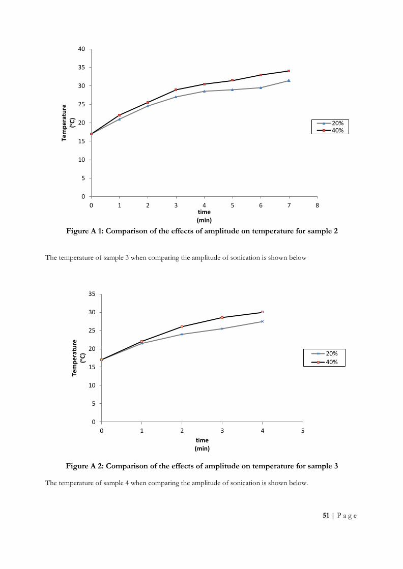
51 | P a g e
Figure A 1: Comparison of the effects of amplitude on temperature for sample 2
The temperature of sample 3 when comparing the amplitude of sonication is shown below
Figure A 2: Comparison of the effects of amplitude on temperature for sample 3
The temperature of sample 4 when comparing the amplitude of sonication is shown below.
0
5
10
15
20
25
30
35
40
0 1 2 3 4 5 6 7 8
Tem
pe
ratu
re
(ºC
)
time (min)
20%40%
0
5
10
15
20
25
30
35
0 1 2 3 4 5
Tem
pe
ratu
re
(ºC
)
time (min)
20%
40%

52 | P a g e
Figure A 3: Comparison of the effects of amplitude on temperature for sample 4
The temperature of sample 5 when comparing the amplitude of sonication is shown below.
Figure A 4: Comparison of the effects of amplitude on temperature for sample 5
The temperature of sample 6 when comparing the amplitude of sonication is shown below.
0
5
10
15
20
25
30
35
0 1 2 3 4 5 6
Tem
pe
ratu
re
ºᵒC)
time (min)
20%40%
0
5
10
15
20
25
30
35
40
0 1 2 3 4 5 6
Tem
pe
ratu
re
(ºC
)
time (min)
20%40%

53 | P a g e
Figure A 5: Comparison of the effects of amplitude on temperature for sample 6
Table A 3: Raw data for before sonication
Component Sample 1 Sample 2 Sample 3 Sample 4 Sample 5 Sample 6
Volume fraction
Ethanol 0.300 0.400 0.440 0.500 0.550 0.590
Petrol 0.670 0.550 0.510 0.430 0.370 0.315
Water 0.030 0.050 0.050 0.070 0.080 0.095
Mass fraction
Ethanol 0.309 0.407 0.447 0.503 0.550 0.586
Petrol 0.652 0.528 0.489 0.408 0.370 0.295
Water 0.039 0.064 0.064 0.089 0.101 0.119
Phase
Petrol (g/L) 115.640 126.368 98.033 70.732 67.510 64.450
Water(E+W) 248.994 263.311 286.620 285.802 306.524 327.089
Water (E) 218.994 213.311 236.620 215.802 226.524 232.089
E (Pet/Wat) 0.464 0.480 0.342 0.247 0.220 0.197
Energy P 33.02986 32.87906 33.277358 33.66113 33.70642 33.74944
Energy E 6.536313 6.366704 7.0623962 6.441048 6.761058 6.927175
0
5
10
15
20
25
30
35
0 1 2 3 4 5
Tem
pe
ratu
re
(ºC
)
time (min)
20%40%

54 | P a g e
Table A 4: Raw data for 15ºC water bath
Sample 1 Sample 5 Sample 3 Sample 4 Sample 5 Sample 6
Phase
Petrol (g/L) 167.3659 173.2411 141.6115 98.21301 94.09331 69.95009
Water(E+W) 209.7115 221.5798 237.8969 271.8504 289.7714 308.3381
Water (E) 179.7115 171.5798 187.8969 201.8504 209.7714 213.3381
Pet/Wat 0.798077 0.781845 0.595264 0.361276 0.324716 0.226862
Volume P 787.9689 780.5258 820.5965 875.5767 880.7959 911.3822
Volume E 212.0311 219.4742 179.4035 124.4233 119.2041 88.61777
Energy(kJ/L) P 32.30275 32.22017 32.66478 33.27483 33.33274 33.67212
Energy(kJ/L) W 5.363849 5.121142 5.608158 6.02463 6.261047 6.367502
Table A 5: Raw data for 25ºC water bath
Sample 1 Sample 2 Sample 3 Sample 4 Sample 5 Sample 6
Phase
Petrol (g/L) 167.3659 117.9307 141.6115 254.3134 94.09331 69.95009
Water(E+W) 209.7115 238.2959 237.8969 214.1295 289.7714 308.3381
Water (E) 179.7115 188.2959 187.8969 144.1295 209.7714 213.3381
Pet/Wat 0.798077 0.494892 0.595264 1.187662 0.324716 0.226862
Volume P 787.9689 850.5969 820.5965 677.8176 880.7959 911.3822
Volume E 212.0311 149.4031 179.4035 322.1824 119.2041 88.61777
Energy(kJ/L) P 32.30275 32.99766 32.66478 31.08054 33.33274 33.67212
Energy(kJ/L) W 5.363849 5.620069 5.608158 4.301833 6.261047 6.367502
Table A 6: Raw data for 35ºC water bath
Sample 1 Sample 2 Sample 3 Sample 4 Sample 5 Sample 6
Ethanol g/ml 0.236804 0.315738 0.347312 0.394673 0.43414 0.465714
Petrol g/ml 0.49895 0.409586 0.379798 0.320221 0.275539 0.234581
Water g/ml 0.03 0.05 0.05 0.07 0.08 0.095
Total mass 0.765754 0.775324 0.77711 0.784894 0.78968 0.795295
Energy W 7.067884 9.423845 10.36623 11.77981 12.95779 13.90017
Energy P 23.21912 19.06047 17.67426 14.90182 12.8225 10.91645
Total energy/ L 30.28701 28.48432 28.04049 26.68163 25.78029 24.81662
Table A 7: Raw data for temperatures collected at 20% amplitude
Time Sample 1 Sample 2 Sample 3 Sample 4 Sample 5 Sample 6
0 16.8 17 17 18 18 18.5
1 17.8 21 21.5 22 23 22.5
2 20 24.5 24 24 26 24
3 22 27 25.5 27 29 27
4 23 28.5 27.5 30 32.5 29.5

55 | P a g e
Table A 8: Raw data for temperatures collected at 40% amplitude
Time Sample 1 Sample 2 Sample 3 Sample 4 Sample 5 Sample 6
0 16.8 17 17 18 18 18.5
1 22 22 22 22 24 23
2 25.5 25.5 26 25.5 28 26.5
3 28 29 28.5 29 30.5 28.5
4 29 30.5 30 31 31.5 30
5 31.5 31.5 33 34
6 33 33 36
7 34
Table A 9: Viscosities of the pure components, www.engineeringtoolbox.com
Component Viscocity (cSt)
Water 1.13
Petrol 0.88
Ethanol 1.52