Embed Size (px)
Citation preview
Reliable Computation of Homogeneous Azeotropes
Robert W. Maier, Joan F. Brennecke and Mark A. Stadtherr1
Department of Chemical EngineeringUniversity of Notre DameNotre Dame, IN 46556
USA
January 1998(revised, May 1988)
Keywords: Azeotropes, Phase Equilibrium, Separations, Interval Analysis
1author to whom all correspondence should be addressed; Fax: (219) 631-8366; Phone: (219) 631-9318;E-mail: [email protected]
Abstract
The determination of the existence and composition of homogeneous azeotropes is important
both from both theoretical and practical standpoints in the analysis of phase behavior and in the
synthesis and design of separation systems. We present here a new method for reliably locating any
and all homogeneous azeotropes for multicomponent mixtures. The method also veri�es the nonex-
istence of homogeneous azeotropes if none are present. The method is based on interval analysis,
in particular an interval Newton/generalized bisection algorithm that provides a mathematical and
computational guarantee that all azeotropes are located. The technique is general purpose and
can be applied in connection with any thermodynamic models. We illustrate the technique here in
several example problems using the Wilson, NRTL, and UNIQUAC activity coeÆcient models.
1 Introduction
The determination of the existence and composition of homogeneous azeotropes is important
both from theoretical and practical standpoints. An important test of thermodynamic models is
whether or not known azeotropes are predicted, and whether or not they are predicted accurately.
Model parameters can be �ne tuned by comparing the model predictions with known azeotropic
data. The determination of azeotropes strictly from experiment alone can be expensive. Predicting
azeotropes computationally is one method of reducing this cost, as the computational results can
be used to narrow the experimental search space. Of course, knowledge of azeotropes is important
since they often present limitations in separation operations which must be known. Furthermore,
this knowledge can be used in the construction of residue curve maps for the synthesis and design
of separation operations.
The problem of computing homogeneous azeotropes frommodels of phase behavior has attracted
signi�cant attention (e.g., Aristovich and Stepanova, 1970; Teja and Rowlinson, 1973; Wang and
Whiting, 1986; Chapman and Goodwin, 1993), and has been reviewed recently by Widagdo and
Seider (1996). The highly nonlinear form of the thermodynamic equations for phase equilibrium
makes the computation of azeotropes a particularly diÆcult problem. In order to be most useful, a
computational method for locating azeotropes must be completely reliable, capable of �nding (or,
more precisely, enclosing within a very narrow interval) all azeotropes when one or more exists, and
capable of verifying (within limits of machine precision) when none exist. Because of the diÆculties
in providing such guarantees, there has been considerable recent interest in developing more reliable
techniques for the computation of homogeneous azeotropes. For example, Fidkowski et al. (1993)
and Westerberg and Wahnscha�t (1996) have presented continuation methods for this purpose,
1
and Okasinski and Doherty (1997) have used a similar approach for �nding reactive azeotropes.
While these methods are very reliable, a drawback is that they can not completely guarantee that
all azeotropes have been enclosed. More recently, Maranas et al. (1996) and Harding et al. (1997)
have used a powerful global optimization procedure; it is based on branch and bound with convex
underestimating functions that are continuously re�ned as the domain in which azeotropes may
occur is narrowed. This technique does provide a mathematical guarantee that all azeotropes
have been enclosed. Harding et al. (1997) have developed appropriate convex underestimating
functions for several speci�c thermodynamic models. While global optimization methods based
on branch and bound can provide mathematical guarantees, in principle this guarantee can be
lost computationally if the technique is implemented in oating point arithmetic, due to rounding
error. In practice, however, if variables are well scaled, as is the case here, this is unlikely to cause
problems.
We describe here a new approach for reliably enclosing all homogeneous azeotropes of mul-
ticomponent mixtures, and for verifying when none exist. The technique is based on interval
analysis, in particular the use of an interval Newton/generalized bisection algorithm. The method
is mathematically and computationally guaranteed to enclose any and all homogeneous azeotropes,
automatically dealing with rounding error, and requiring no initial starting point. It does not re-
quire the construction of model-speci�c convex underestimating functions, is general purpose, and
can be applied in connection with any thermodynamic model. In the work presented here, the
vapor phase is modeled as ideal, and the Wilson, NRTL, and UNIQUAC activity coeÆcient models
are used to describe the liquid phase.
In the next section, we present the mathematical formulation of the problem. In Section 3, we
describe the interval Newton/generalized bisection method used. Finally, in Section 4 we present
2
the results for several test problems, and in Section 5 give concluding remarks concerning this
study.
2 Mathematical Formulation
At a homogeneous azeotrope, vapor and liquid phases of the same composition are in equilib-
rium. For a mixture of N components, the equilibrium condition can be written in terms of the
equality of fugacities,
f̂Vi = f̂Li ; 8i 2 C
where f̂Vi refers to the fugacity of component i in the vapor phase, f̂Li refers to the fugacity of
component i in the liquid solution, and C is the set of components in question. These solution
fugacities can in turn be written as
yi�̂Vi P = xi
Li f
Li ; 8i 2 C
where P is the system pressure, �̂Vi is the mixture fugacity coeÆcient of component i in the vapor
phase, Li is the activity coeÆcient of component i in the liquid phase, fLi is the pure component
fugacity of component i in the liquid phase, yi is the mole fraction of component i in the vapor
phase, and xi is the mole fraction of component i in the liquid phase. Assuming ideal vapor behavior
and Poynting correction factors of one, this becomes
yiP = xi Li P
sati ; 8i 2 C
where P sati is the vapor pressure of component i. Using the homogeneous azeotropy condition
xi = yi, 8i 2 C, now yields
xi(P � Li Psati ) = 0; 8i 2 C : (1)
3
This has the solution xi = 0 or P = Li Psati . It is convenient to rewrite the latter as lnP � lnP sat
i �
ln Li = 0, since the vapor pressure and activity coeÆcient relationships are typically expressed in
terms of their logarithms. Equation (1) can now be expressed as
xi (lnP � lnP sati (T )� ln Li (T )) = 0; 8i 2 C (2)
where we have emphasized the temperature dependence of P sati and Li . This equation, and the
constraint that the mole fractions sum to one
NXi=1
xi � 1 = 0 (3)
constitute an (N + 1) � (N + 1) set of nonlinear equations that can be solved for the azeotropic
composition(s) and temperature(s). We refer to equations (2) and (3) as the simultaneous formu-
lation. This is the formulation used by Fidkowski et al. (1993), and is one of the formulations used
by Harding et al. (1997). Solving (2) and (3) we will simultaneously obtain all k-ary azeotropes
(k � N) in the system, as well as trivial roots representing the pure components. Clearly, this
equation system may have many roots, and a solution method guaranteed to enclose all the roots
is required.
If we assume that there is a set of k components Cnz for which xi 6= 0, then for this set of k
nonzero components, equation (2) can be rewritten
lnP � lnP sati (T )� ln Li (T ) = 0; 8i 2 Cnz: (4)
We refer to equations (3) and (4) as the sequential formulation. This is one of the formulations used
by Harding et al. (1997), and is similar to the approach used byWesterberg andWahnscha�t (1996).
Solving this (k+1)�(k+1) system, we will obtain all k-ary azeotropes for the chosen component set
Cnz. To �nd all the azeotropes in the original N component system, a sequence (unordered) of such
4
systems must be solved, one for each combination of k components, k = 2; : : : ; N . These equation
systems may have multiple roots or no roots at all. A solution method is required that is guaranteed
to enclose all roots and that is also capable of verifying when none exist. Both the simultaneous
and sequential formulations are considered here, and their relative eÆciency compared.
To model the temperature dependence of P sati (T ) we use the Antoine equation
log10 Psati = Ai �
Bi
T + Ci
:
This is a dimensional equation with P sati in mmHg and T in ÆC. Values used for the constants Ai,
Bi and Ci in the example problems below were taken from Gmehling et al. (1977-1990), and are
listed in Table A1 in the Appendix.
In many cases, the temperature dependence of P sati (T ) is signi�cantly stronger than the tem-
perature dependence of Li (T ), which arises only in the temperature dependence of the binary
interaction parameters in the activity coeÆcient model used. Thus, as done by Harding et al.
(1997), it is not unreasonable to evaluate Li (T ) at some reference temperature TREF and then
treat it as independent of temperature, instead of using a fully temperature dependent Li (T )
model. Assuming a good guess of TREF is made, this approach may provide good estimates for the
azeotropes in the fully temperature dependent model. However, there is no guarantee of this, and
it is possible that the number of azeotropes found in the TREF -based model will not be the same as
the number of azeotropes that exist in the fully temperature dependent model, even if a relatively
good guess of TREF has been made. This is demonstrated in Problem 5 below.
The method described here is model independent and can be applied in connection with any
models of phase behavior. For the �rst �ve example problems below, one of the activity coeÆcient
models used is the Wilson equation. In this model, the nonsymmetric binary interaction parameters
5
�ij = (Vj=Vi) exp(�Aij=RT ) are based on energy parameters Aij , values of which are reported as
constants or as linear functions of temperature. For the problems below, we use the constants
reported in Gmehling et al. (1977-1990), as listed in Table A2. For the saturated liquid molar
volumes Vi, Gmehling et al. (1977-1990) use temperature independent constants. However, to be
consistent with Harding et al. (1997), we use a modi�ed Rackett equation (Yamada and Gunn,
1973),
Vi = VscriZ(1�TRi)
2
7
cri ;
where TRiis the reduced temperature of component i. The other quantities are Vscri , the scaling
volume for component i, and Zcri , the critical compressibility of component i for the Rackett
equation, and are given by
Vscri = V 0
i Z�
�1�T 0
Ri
�2
7
cri ;
and
Zcri = 0:29056 � 0:08775!i;
where V 0
i is the molar volume for component i at T 0
Ri, a reference reduced temperature for which
the molar volume of component i is accurately known, and !i is the acentric factor for component
i. The values used for these three parameters are given in Table A3, and were taken from Reid et
al. (1987) and Lide (1995).
For the �rst �ve example problems below, a second activity coeÆcient model used is the NRTL
equation. In this model, the binary interaction parameters �ij = Aij=RT and Gij = exp(��ij�ij)
are based on constants �ij = �ji and energy parameters Aij , values of which are reported as
constants or functions of temperature. For the problems below, we use the constant Aij and �ij
values reported in Gmehling et al. (1977-1990), as listed in Table A4.
6
In the last three example problems, the activity coeÆcient model used is the UNIQUAC equation
as modi�ed by Anderson and Prausnitz (1978), with coordination number z = 10. The binary
interaction parameters �ij = exp(�Aij=RT ) are computed from energy parameters Aij, values of
which are reported as constants or as functions of temperature. For the problems below, we use
the Aij constants, as well as the pure component ri, qi and q0i constants, reported in Gmehling et
al. (1977-1990) and Prausnitz et al. (1986), as listed in Tables A5 and A6.
Finally, it should be noted that because solutions of the equifugacity equations may not be stable
phases (the liquid may split), any solutions enclosed using either of the formulations described
above should next be checked for phase stability. This can be reliably done using either an interval
approach (Stadtherr et al., 1995) or a branch and bound global optimization approach (McDonald
and Floudas, 1995).
3 Solution Method
We apply here interval mathematics, in particular an interval Newton/generalized bisection
(IN/GB) technique, to �nd enclosures for all homogeneous azeotropes. Recent monographs which
introduce interval computations include those of Neumaier (1990), Hansen (1992) and Kearfott
(1996). The IN/GB algorithm used here has been summarized by Hua et al. (1998) and given in
more detail by Schnepper and Stadtherr (1996). Properly implemented, this technique provides
the power to �nd, with mathematical and computational certainty, enclosures of all solutions of
a system of nonlinear equations (Neumaier, 1990; Kearfott and Novoa, 1990), provided only that
initial upper and lower bounds are available for all variables. This is made possible through the use
of the existence and uniqueness test provided by the interval Newton method. Our implementation
of the IN/GB method for the homogeneous azeotrope problem is based on appropriately modi-
7
�ed FORTRAN-77 routines from the packages INTBIS (Kearfott and Novoa, 1990) and INTLIB
(Kearfott et al., 1994).
In the past, interval techniques were not widely used. One reason for this was that the theoretical
guarantees on solution enclosures often came at a very large cost in additional time relative to faster,
but not guaranteed, local methods. However, with continuing improvements in methodology (e.g.,
Kearfott, 1996), and continuing advances in computation speed and parallel computing, both the
premium paid to obtain the guarantee, as well as the absolute execution time required, have shrunk
dramatically.
One method for improving the computational eÆciency of the interval approach is to develop
interval extensions that are computationally inexpensive and that more tightly enclose the range
of a function than the natural interval extension. For an arbitrary function f(x) over an interval
X = (X1;X2; :::;Xn)T , with n real interval components Xi, the interval extension F(X) encloses
all values of f(x) for x 2 X; that is, it encloses the range of f(x) over X. Often, the natural interval
extension, that is the enclosure F(X) computed using interval arithmetic, is wider than the actual
range of f(x) overX. Because of the complexity of the functions to be solved here, the use of interval
arithmetic may lead to signi�cant overestimation of the true range of the functions. One simple way
to alleviate this diÆculty in solving the azeotrope problem is to focus on tightening the enclosure
when computing interval extensions of mole fraction weighted averages, such as �s =Pn
i=1 xisi,
where the si are constants, since such expressions occur frequently in activity coeÆcient models.
The natural interval extension of �s will yield the true range of the expression in the space in
which all the mole fraction variables xi are independent. However, the range can be tightened by
considering the constraint that the mole fractions must sum to one. Thus we use a constrained
space interval extension of �s. One approach for doing this is simply to eliminate one of the mole
8
fraction variables, say xn. Then an enclosure for the range of �s in the constrained space can be
determined by computing the natural interval extension of sn+Pn�1
i=1 (si�sn)xi. However, as noted
by Hua et al. (1998) and Tessier (1997), this may not yield the sharpest possible bounds on �s in
the constrained space. For determining the exact (within roundout) bounds on �s in the constrained
space, Tessier (1997) and Hua et al. (1998) have presented a very simple method, and that method
was used in obtaining the results presented here. A comparison of computation times with and
without use of these constrained space interval extensions for mole fraction weighted averages is
given below using Problems 6{8.
4 Results
The computational results for several example problems are given below. In Problems 1{5,
both the Wilson and NRTL equations are used to model the liquid phase activity coeÆcients,
and in Problems 6{8 the UNIQUAC equation is used. For each problem solved we present the
azeotrope(s) found, as well as the CPU time required. The CPU times are given in seconds on a
Sun Ultra 1/140 workstation. Each problem was solved using a fully temperature dependent activity
coeÆcient model, and also solved using the approach in which the activity coeÆcients are evaluated
at some reference temperature TREF and then treated as temperature independent (e.g., Harding
et al., 1997). Unless otherwise noted, the reference temperatures used are those used by Harding
et al. (1997). Since these reference temperatures are very close approximations to the actual
azeotropic temperatures, the azeotropic compostions and temperatures found using the TREF -
based approach are not signi�cantly di�erent from the results of the fully temperature dependent
approach. Thus, in the tables of results, only the latter results are given, though computation times
for both approaches are provided. However, there are dangers in using the TREF -based approach,
9
even when the reference temperature is quite close to the azeotropic temperature, as emphasized
in Problem 5.
The values of the energy parameters Aij used in each model were taken from Gmehling et al.
(1977-1990) and are listed in Tables A2, A4 and A6. For many binaries, Gmehling et al. (1977-
1990) present multiple data sets and thus a choice of parameter values. In some cases, as noted
below, our computed results do not match those of Harding et al. (1997). This is presumably due
to their use of a di�erent set of parameter values.
It should be noted that, while point approximations of the azeotropic compositions and tem-
perature are reported in the tables here, we have actually determined veri�ed enclosures of each
root. Each such enclosure is a very narrow interval known to contain a unique root, based on the
interval-Newton uniqueness test. The initial interval used for all mole fraction variables was [0, 1].
The initial interval used for temperature was [10, 100] ÆC, except for Problem 4, in which it is [100,
200] ÆC. These are the same initial temperature ranges used by Harding et al. (1997). Note that no
initial starting points are required. Unless noted otherwise, the ranges of all mole fraction weighted
averages were determined using the constrained space interval extension discussed above. Detailed
results for each problem are given in Tables 2{11 for the Wilson and NRTL equation problems
and in Tables 14{16 for the UNIQUAC equation problems. Table 17 gives a summary of the total
computation time required for each problem.
In addition to presenting the azeotropes and computation times, we also will consider in this
section: 1. the relative computational expense of the sequential and simultaneous formulations; 2.
the diÆculties that may arise in using the TREF -based approach for the temperature dependence of
the activity coeÆcients; and 3. the e�ect on computation time of using constrained space interval
extensions to tighten the evaluation of function ranges involving mole fraction weighted averages.
10
4.1 Wilson and NRTL Equations
The �rst �ve example problems were solved using both the Wilson equation and the NRTL
equation as liquid phase activity coeÆcient models. These problems were previously solved by
Fidkowski et al. (1993) using the Wilson equation, and by Harding et al. (1997) using both the
Wilson and NRTL equations. Harding et al. (1997) used the reference temperature approach in
their calculations; Fidkowski et al. (1993) do not state whether or not they considered the binary
interaction parameters to be constants at a reference temperature or functions of temperature.
Before proceeding to the detailed results on individual problems, we �rst consider the relative
computational eÆciency of the sequential [equations (3) and (4)] and simultaneous [equations (2)
and (3)] problem formulations. For this comparison we used the Wilson equation with reference
temperature case for each of these �ve examples. Results of this comparison are summarized in
Table 1, which gives the total time required for each problem and formulation, as well as the
number of leaves that occur in the binary tree generated in the bisection process. The results
clearly indicate that use of the sequential formulation is much more eÆcient. This same conclusion
was also reached by Harding et al. (1997) when they performed a similar comparison using their
solution method. As suggested by Harding et al. (1997), one reason for this may be the increased
complexity introduced by the additional factor of xi in equation (2) in comparison to equation (4).
It is also likely that another reason for this is that, when the simultaneous formulation is used,
there are also trivial roots, corresponding to each pure component at its boiling temperature, that
are found using the interval approach, since it �nds enclosures of all roots of the equation system.
In obtaining all of the results presented below (Tables 2{17), the sequential approach was used.
However, in all cases, the same azeotropic compositions and temperatures were also found using
the simultaneous approach. In reporting the results for the sequential approach, the CPU time
11
required to solve each problem in the sequence is reported, along with the total time.
4.1.1 Problem 1
The �rst example problem is a four component system consisting of methanol, benzene, i-
propanol, and n-propanol at 1 atmosphere. Table 2 shows the computational results for this system
when the Wilson equation is used, and Table 3 when the NRTL equation is used. In all cases, three
binary azeotropes were found, corresponding to each of the binary pairs that include benzene, and
no higher order azeotropes were located. These results correspond closely to experimental data
(Gmehling et al., 1994). While comparisons to experimental results are interesting, it should be
emphasized that such comparisons serve only as a measure of the accuracy of the model solved,
and not of the e�ectiveness of the solution method used. The results also are in agreement with
both Fidkowski et al. (1993) and Harding et al. (1997) for the Wilson equation cases. For the
NRTL equation, the computed methanol/benzene binary azeotrope di�ers signi�cantly from the
result obtained by Harding et al. (1997), presumably due to the use of a di�erent set of model
parameters. As might be expected, the use of a fully temperature dependent activity coeÆcient
model increased computation times, most dramatically in the case of the Wilson equation. In
general, the use of the NRTL equation was more expensive than the Wilson equation, especially
in the reference temperature case. The computation times for �nding the binary azeotropes in the
reference temperature cases are signi�cantly less than those reported by Harding et al. (1997),
even after adjusting for di�erence in the machines used. However, no meaningful comparisons
along these lines can be made, since Harding et al. (1997) implemented their solution technique
using GAMS, which adds signi�cant computational overhead. Furthermore, Harding et al. (1997)
do not report the computation time required to con�rm that there are no ternary or quaternary
12
azeotropes, or binary azeotropes for three of the binary pairs. As can clearly be seen, the expense
of verifying the nonexistence of azeotropes comprises the bulk of computation time for solving this
problem.
4.1.2 Problem 2
The second problem is the binary system of benzene and hexa uorobenzene at 0.2 atmospheres.
Table 4 shows the computational results for this system when the Wilson equation is used, and
Table 5 when the NRTL equation is used. Although only a two component system, it contains two
distinct azeotropes. The results shown here for the Wilson equation are in good agreement with
those of Fidkowski et al. (1993) and Harding et al. (1997). Neither group reported results for
the NRTL equation. This example demonstrates the ability of the interval method to easily �nd
multiple azeotropes when they exist for a given set of nonzero components.
4.1.3 Problem 3
The third example problem is the ternary system consisting of ethanol, methyl ethyl ketone, and
water at 1 atmosphere. Table 6 shows the computational results for this system when the Wilson
equation is used, and Table 7 when the NRTL equation is used. Experimentally, this system
contains one binary azeotrope for each pair of components and one ternary azeotrope (Gmehling et
al., 1994). The results for the binary azeotropes are fairly consistent with experimental data, while
the results for the ternary azeotrope are less accurate in this regard, indicating some shortcomings in
the models solved. Our computed results are consistent in all respects with the results of Fidkowski
et al. (1993) and Harding et al. (1997).
13
4.1.4 Problem 4
The fourth problem is a ternary system of acetone, chloroform, and methanol at 15.8 atmo-
spheres. Tables 8 and 9 show the computational results for this system for the Wilson and NRTL
models, respectively. This ternary system was found to contain one azeotrope for each of the binary
pairs, and no ternary azeotropes. These results are consistent with those obtained by Harding et
al. (1997) using their branch and bound technique, and also to the results obtained by Fidkowski et
al. (1993) for the Wilson equation. In the temperature dependent case, this was the only example
problem in which use of the NRTL model was faster than use of the Wilson model.
4.1.5 Problem 5
The �fth problem is a quinary system consisting of acetone, chloroform, methanol, ethanol,
and benzene at 1 atmosphere. Tables 10 and 11 show the computational results for this example
for the Wilson and NRTL models, respectively. Experimentally, this quinary system is reported
to have 6 binary azeotropes, 3 ternary azeotropes, and 1 quaternary azeotrope (Gmehling et al.,
1994). In each set of computed results, all of these azeotropes were found except for a ternary
azeotrope involving chloroform, methanol, and benzene. Thus neither model appears to provide a
completely accurate picture of this system. The computed results given here again match closely
those of Fidkowski et al. (1993) and Harding et al. (1997). It is well worth noting again here that
the bulk of the computation time is spent in verifying the nonexistence of azeotropes.
In the results presented so far, there has been little signi�cant di�erence in azeotrope locations
obtained using the reference temperature approach and using the fully temperature dependent
approach, and thus only the latter were given in Tables 2{11. Essentially, the TREF values used
proved to be good approximations of the azeotropic temperatures. However, as noted above, even
14
with a relatively good guess of the TREF value to use, there is no guarantee that that the number
of azeotropes found in the TREF -based model will be the same as the number of azeotropes that
exist in the fully temperature dependent model. This can be seen in the case of the quaternary
azeotrope (acetone/chloroform/methanol/benzene) in this problem. Table 12 shows the e�ect of
using di�erent values of TREF on the location of this azeotrope when the NRTL equation is used.
For this problem, the azeotrope in the fully temperature dependent model is found to be at 57.05 ÆC.
As expected, setting TREF = 57:05 ÆC and using the reference temperature approach to compute
the azeotrope yields the same result, as shown in the �rst row of Table 12. However, as TREF
is increased beyond 57.05 ÆC, the mole fraction of benzene decreases to zero, at which point no
quaternary azeotrope is found. This shows that, although the use of a reference temperature is
faster, it is possible to miss azeotropes when this approach is used. In this case, just a 20 ÆC
change in the reference temperature results in loss of an azeotrope. In attempting to use the
reference temperature approach, one can imagine using an algorithm in which an initial value of
TREF is chosen to compute an azeotrope, after which the computed azeotropic temperature is then
used as TREF and the azeotrope computed again, etc. However, such an approach will fail if at the
initial reference temperature the azeotrope sought does not exist. One cannot tell how close TREF
must be to the azeotrope in order to ensure that it will be found. Therefore, there is no guarantee
using the reference temperature approach that the azeotropes existing in the fully temperature
dependent model will be found.
4.2 UNIQUAC Equation
The �nal three example problems were solved using the UNIQUAC equation as the activity
coeÆcient model, with both the reference temperature and temperature dependent approaches.
15
These problems were also considered by Harding et al. (1997), who use the reference temperature
approach.
Before proceeding to the detailed results on individual problems, we �rst consider the e�ect of
using constrained space interval extensions instead of natural interval extensions for determining the
range of the mole fraction weighted averages occurring the model. As noted above, this appears
to be a simple way to improve the computational eÆciency of the method used here. For this
comparison we used the reference temperature case for each of the three UNIQUAC examples.
Results of this comparison are summarized in Table 13, which gives the total time required for
each problem and interval extension, as well as the number of leaves that occur in the binary
tree generated in the bisection process. The results clearly indicate that use of the constrained
space interval extensions for mole fraction weighted averages results in a dramatic increase in
computational eÆciency. The results in all other tables are for the case in which the constrained
space interval extensions are used.
4.2.1 Problem 6
The �rst UNIQUAC problem is a ternary system consisting of benzene, ethanol, and water at
1 atmosphere. Table 14 shows the computational results for this example. Experimentally, this
ternary system is known to have one binary azeotrope for each binary pair, but no homogeneous
ternary azeotrope (Gmehling et al., 1994). The computed results for this system match the exper-
imental data well in all respects. However, our computed results di�er signi�cantly from those of
Harding et al. (1997), in that they compute a ternary azeotrope, while we do not. Presumably,
this is due to some di�erence in the model parameters used. As in the previous examples, use of
the temperature dependent approach is more expensive computationally than the reference tem-
16
perature approach. As in the case of the NRTL equation, the increased expense is less dramatic
(about a factor of two) than in the problems using the Wilson equation.
4.2.2 Problem 7
This problem is a quaternary system consisting of ethanol, methylcyclopentane, benzene, and
hexane at 1 atmosphere. Table 15 shows the computational results for this problem. Experimen-
tally, this quaternary system is reported to have 5 binary azeotropes, and none of higher order
(Gmehling et al., 1994). The computed results for this system match these experimental results
quite well. Again, however, there are signi�cant deviations between our computed results and those
of Harding et al. (1997), as they compute azeotropes for all of the six cases in which we �nd none,
presumably due to di�erences in model parameters used.
4.2.3 Problem 8
The �nal example is a ternary system containing acetone, methyl acetate, and ethyl formate
at 1 atmosphere. Table 16 shows the computational results for this problem. Experimentally, this
ternary system is known to have one binary azeotrope (acetone/methyl acetate) and one ternary
azeotrope (Gmehling et al., 1994). The computed results for this system match the experimental
data closely in all respects. As in the previous problems using the UNIQUAC model, our results
and those of Harding et al. (1997) di�er, as they compute an azeotrope for the acetone/ethyl
formate pair and we do not. Again, this is presumably due to di�erences in model parameters
used.
17
5 Concluding Remarks
We have described here a new method for reliably locating all homogeneous azeotropes in
multicomponent mixtures, and for verifying their nonexistence if none are present. The method
is based on interval analysis, in particular an interval Newton/generalized bisection algorithm,
which provides a mathematical and computational guarantee that all azeotropes are enclosed.
We applied the technique here to several problems in which the Wilson, NRTL, and UNIQUAC
activity coeÆcient models were used. However, the technique is general purpose and can be applied
in connection with any thermodynamic models.
Both a sequential and simultaneous formulation of the problem were considered, with the se-
quential proving to be the most eÆcient computationally (Table 1), as also noted by Harding et
al. (1997). The use of a constrained space interval extension for �nding exact (within roundout)
bounds on mole fraction weighted averages greatly improves the computational eÆciency of the
method, as shown is on Problems 6{8 (Table 13). We also considered two approaches for handling
the temperature dependence of the activity coeÆcients, one in which the activity coeÆcient is eval-
uated at a reference temperature and then treated as independent of temperature, and the other
in which a fully temperature dependent activity coeÆcient model is used. A summary of the total
computation times for each problem, given in Table 17, shows that use of the fully temperature
dependent model increases computation times moderately when the NRTL or UNIQUAC equations
are used, but dramatically when the Wilson equation is used. The strong e�ect on the Wilson equa-
tion problems is probably due to the increased complexity of the temperature dependence arising
from the use of the modi�ed Rackett equation. This additional layer of complexity does not occur
in the other models. The reason for use of the temperature dependent approach was demonstrated
18
in Problem 5, in which it was seen how, even using a reference temperature that is within 20 ÆC of
the azeotropic temperature, the use of the reference temperature approach could lead to the failure
to �nd an azeotrope predicted by the fully temperature dependent model. Thus, if a reference
temperature approach is used, one cannot guarantee that all azeotropes have been located. The
ability of the solution method described here to easily handle the fully temperature dependent case
shows the exibility and generality of the approach.
Acknowledgments | This work has been supported in part by the donors of The Petroleum
Research Fund, administered by the ACS, under Grant 30421-AC9, by the National Science Foun-
dation Grants CTS95-22835 and DMI 96-96110, by the Environmental Protection Agency Grant
R824731-01-0, by the Department of Energy Grant DE-FG07-96ER14691, and by a grant from Sun
Microsystems, Inc.
19
References
Anderson, T. F. and J. M. Prausnitz, \Application of the UNIQUAC Equation to Calculation
of Multicomponent Phase Equilibria. 1. Vapor-Liquid Equilibria," Ind. Eng. Chem. Proc.
Des. Dev., 17, 552{561, (1978).
Aristovich, V. Y. and E. I. Stepanova, \Determination of the Existence and Composition of Mul-
ticomponent of Multicomponent Azeotropes by Calculation from Data for Binary Systems,"
Zh. Prikl. Khim. (Leningrad), 43, 2192{2200 (1970).
Chapman, R. G. and S. P. Goodwin, \A General Algorithm for the Calculation of Azeotropes in
Fluid Mixtures," Fluid Phase Equilib., 85, 55{69 (1993).
Fidkowski, Z. T., M. F. Malone and M. F. Doherty, \Computing Azeotropes in Multicomponent
Mixtures," Comput. Chem. Eng., 17, 1141{1155 (1993).
Gmehling, J., U. Onken and W. Arlt, Vapor-Liquid Equilibrium Data Collection, Chemistry Data
Series, Vol. I, Parts 1-8, DECHEMA, Frankfurt/Main, Germany (1977-1990).
Gmehling, J., J. Menke, J. Krafczyk and K. Fischer, Azeotropic Data, VCH: Weinheim, Germany
(1994).
Hansen, E. R., Global Optimization Using Interval Analysis, Marcel Dekkar, Inc., New York, NY
(1992).
Harding, S. T., C. D. Maranas, C. M. McDonald and C. A. Floudas, \Locating All Homogeneous
Azeotropes in Multicomponent Mixtures," Ind. Eng. Chem. Res., 36, 160{178 (1997).
20
Hua, J. Z., J. F. Brennecke and M. A. Stadtherr, \Enhanced Interval Analysis for Phase Stability:
Cubic Equation of State Models," Ind. Eng. Chem. Res., 37, 1519{1527 (1998).
Kearfott, R. B. Rigorous Global Search: Continuous Problems, Kluwer Academic Publishers,
Dordrecht (1996).
Kearfott, R. B. and M. Novoa III, \Algorithm 681: INTBIS, a Portable Interval-Newton / Bisec-
tion Package," ACM Trans. Math. Soft., 16, 152{157 (1990).
Kearfott, R. B. and M. Dawande, K.-S. Du and C.-Y. Hu, \Algorithm 737: INTLIB, A Portable
FORTRAN 77 Interval Standard Function Library," ACM Trans. Math. Software, 20, 447{
459 (1994).
Lide, D. R., Editor, CRC Handbook of Chemistry and Physics, 76th ed., CRC Press, New York,
NY (1995).
Maranas, C. D., C. M. McDonald, S. T. Harding and C. A. Floudas, \Locating All Azeotropes in
Homogeneous Azeotropic Systems," Comput. Chem. Eng., 20, S413{S418 (1996).
McDonald, C. M. and C. A. Floudas, C. A., \Global Optimization for the Phase Stability Prob-
lem," AIChE J., 41, 1798{1814 (1995).
Moore, R. E., Interval Analysis, Prentice-Hall, Englewood Cli�s, NJ (1966).
Neumaier, A., Interval Methods for Systems of Equations, Cambridge University Press, Cam-
bridge, England (1990).
Okasinski, M. J. and M. F. Doherty, \Thermodynamic Behavior of Reactive Azeotropes," AIChE
J., 43, 2227{2238 (1997).
21
Prausnitz, J. M., R. N. Lichtenthaler and E. G. de Azevedo, Molecular Thermodynamics of Fluid-
Phase Equilibria, Prentice-Hall, Englewood Cli�s, NJ (1986).
Reid, R. C., J. M. Prausnitz and B. E. Poling, The Properties of Gases and Liquids, 4th ed.,
McGraw-Hill, Inc., New York, NY (1987).
Schnepper, C. A. and M. A. Stadtherr, \Robust Process Simulation Using Interval Methods,"
Comput. Chem. Eng., 20, 187{199 (1996).
Stadtherr, M. A., C. A. Schnepper and J. F. Brennecke, \Robust Phase Stability Analysis Using
Interval Methods," AIChE Symp. Ser., 91 (304), 356{359 (1995).
Teja, A. S. and J. S. Rowlinson, \The Prediction of the Thermodynamic Properties of Fluids and
Fluid Mixtures - IV. Critical and Azeotropic States," Chem. Eng. Sci., 28, 529{538 (1973).
Tessier, S. R., Enhanced Interval Analysis for Phase Stability: Excess Gibbs Energy Models, Mas-
ter's thesis, University of Notre Dame, Notre Dame, IN, (1997).
Wang, S. and W. B. Whiting, \New Algorithm for Calculation of Azeotropes from Equations of
State," Ind. Eng. Chem. Proc. Des. Dev., 25, 547{551 (1986).
Westerberg, A. W. and O. Wahnscha�t, \The Synthesis of Distillation- Based Separation Sys-
tems," Advances Chem. Eng., 23, 64{170 (1996).
Widagdo, S. and W. D. Seider, \Azeotropic Distillation," AIChE J., 42, 96{130 (1996).
Yamada, T. and R. D. Gunn, \Saturated Liquid Molar Volumes: The Rackett Equation," J.
Chem. Eng. Data, 18, 234{236 (1973).
22
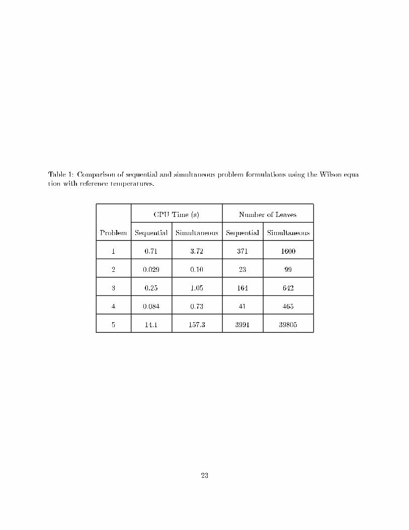
Table 1: Comparison of sequential and simultaneous problem formulations using the Wilson equa-tion with reference temperatures.
CPU Time (s) Number of Leaves
Problem Sequential Simultaneous Sequential Simultaneous
1 0.71 3.72 371 1600
2 0.029 0.10 23 99
3 0.25 1.05 164 642
4 0.084 0.73 41 465
5 14.1 157.3 3991 39805
23

Table 2: Problem 1: Methanol(M)/Benzene(B)/i-Propanol(I)/n-Propanol(N); 1 atm; Wilson Equa-tion.
T -dependent TREF = 71:05ÆC
Components Mole Fraction (M B I N) T (ÆC) CPU Time (s) CPU Time (s)
MB 0.615 0.385 0.000 0.000 58.16 0.067 0.011
MI no azeotrope 0.043 0.006
MN no azeotrope 0.028 0.004
BI 0.000 0.590 0.410 0.000 71.98 0.054 0.009
BN 0.000 0.773 0.000 0.227 76.75 0.056 0.009
IN no azeotrope 0.049 0.009
MBI no azeotrope 0.66 0.077
MBN no azeotrope 0.50 0.047
MIN no azeotrope 0.44 0.032
BIN no azeotrope 0.73 0.077
MBIN no azeotrope 4.67 0.43
total 7.30 0.71
24
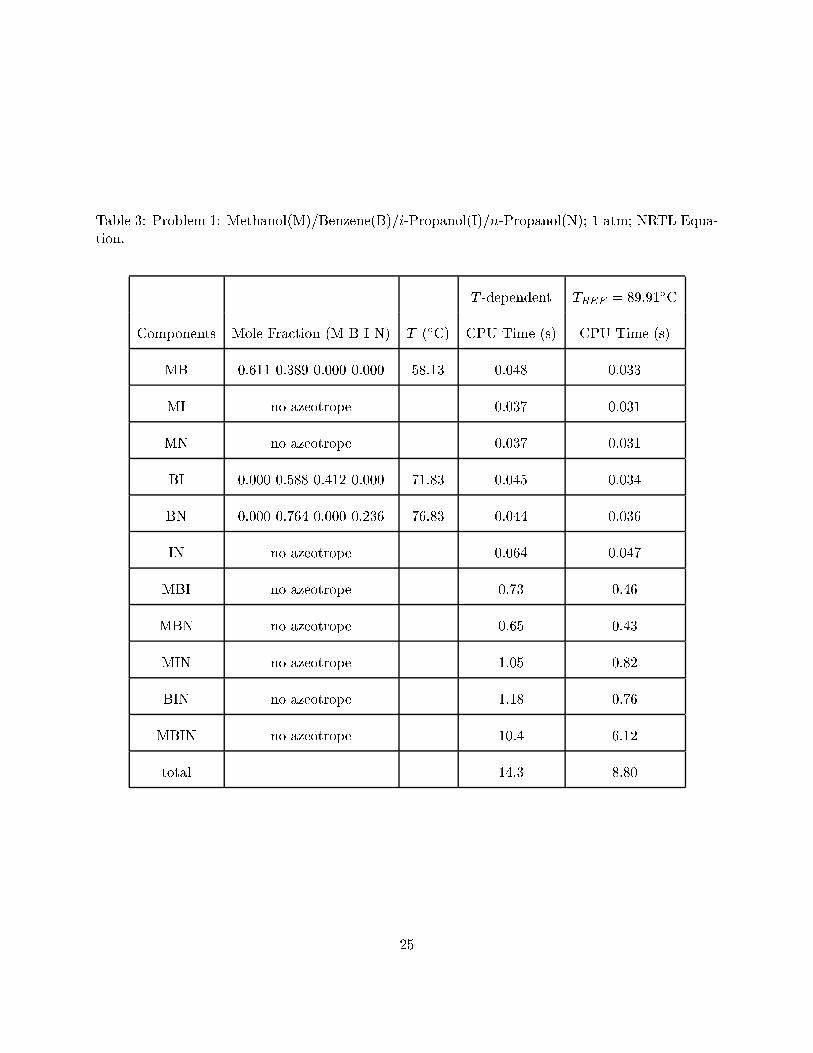
Table 3: Problem 1: Methanol(M)/Benzene(B)/i-Propanol(I)/n-Propanol(N); 1 atm; NRTL Equa-tion.
T -dependent TREF = 89:91ÆC
Components Mole Fraction (M B I N) T (ÆC) CPU Time (s) CPU Time (s)
MB 0.611 0.389 0.000 0.000 58.13 0.048 0.033
MI no azeotrope 0.037 0.031
MN no azeotrope 0.037 0.031
BI 0.000 0.588 0.412 0.000 71.83 0.045 0.034
BN 0.000 0.764 0.000 0.236 76.83 0.044 0.036
IN no azeotrope 0.064 0.047
MBI no azeotrope 0.73 0.46
MBN no azeotrope 0.65 0.43
MIN no azeotrope 1.05 0.82
BIN no azeotrope 1.18 0.76
MBIN no azeotrope 10.4 6.12
total 14.3 8.80
25
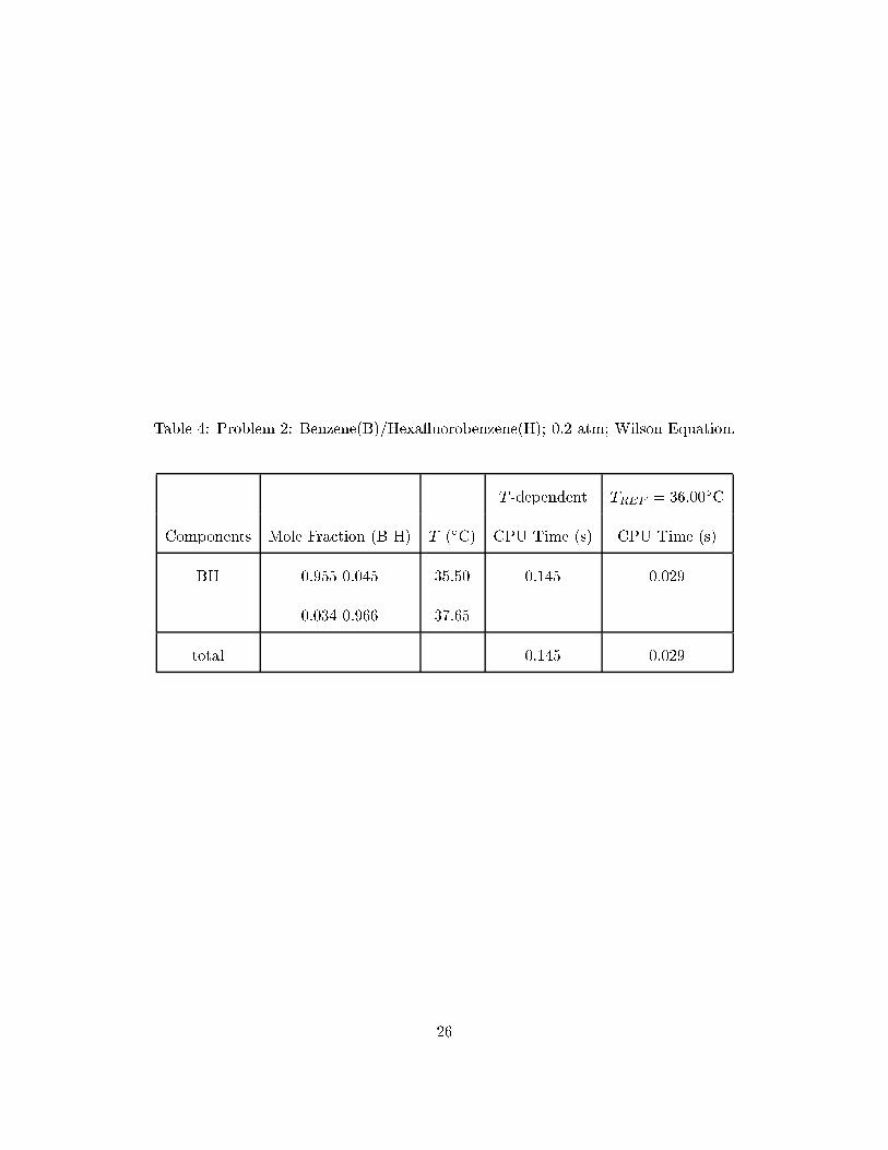
Table 4: Problem 2: Benzene(B)/Hexa uorobenzene(H); 0.2 atm; Wilson Equation.
T -dependent TREF = 36:00ÆC
Components Mole Fraction (B H) T (ÆC) CPU Time (s) CPU Time (s)
BH 0.955 0.045 35.50 0.145 0.029
0.034 0.966 37.65
total 0.145 0.029
26
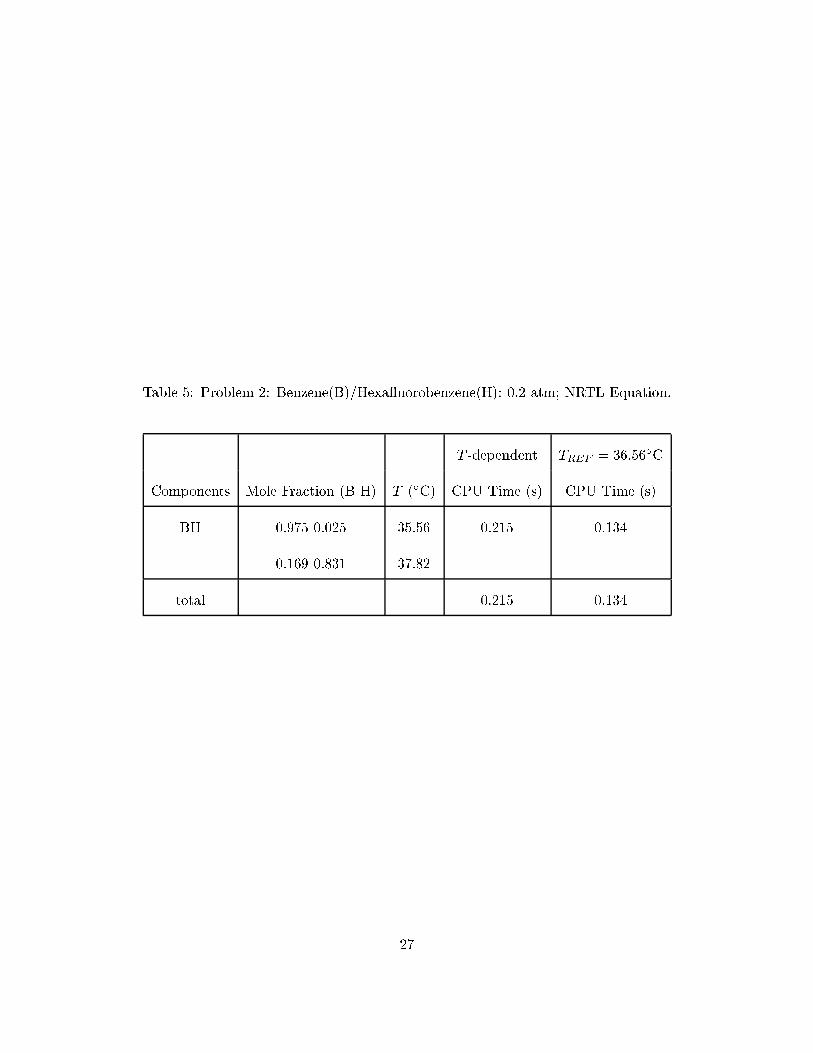
Table 5: Problem 2: Benzene(B)/Hexa uorobenzene(H): 0.2 atm; NRTL Equation.
T -dependent TREF = 36:56ÆC
Components Mole Fraction (B H) T (ÆC) CPU Time (s) CPU Time (s)
BH 0.975 0.025 35.56 0.215 0.134
0.169 0.831 37.82
total 0.215 0.134
27
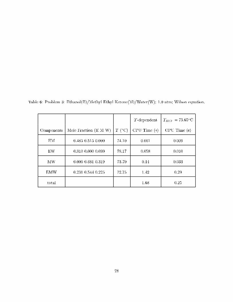
Table 6: Problem 3: Ethanol(E)/Methyl Ethyl Ketone(M)/Water(W); 1.0 atm; Wilson equation.
T -dependent TREF = 73:65ÆC
Components Mole Fraction (E M W) T (ÆC) CPU Time (s) CPU Time (s)
EM 0.485 0.515 0.000 74.10 0.061 0.009
EW 0.910 0.000 0.090 78.17 0.058 0.010
MW 0.000 0.681 0.319 73.70 0.14 0.033
EMW 0.231 0.544 0.225 72.75 1.42 0.20
total 1.68 0.25
28
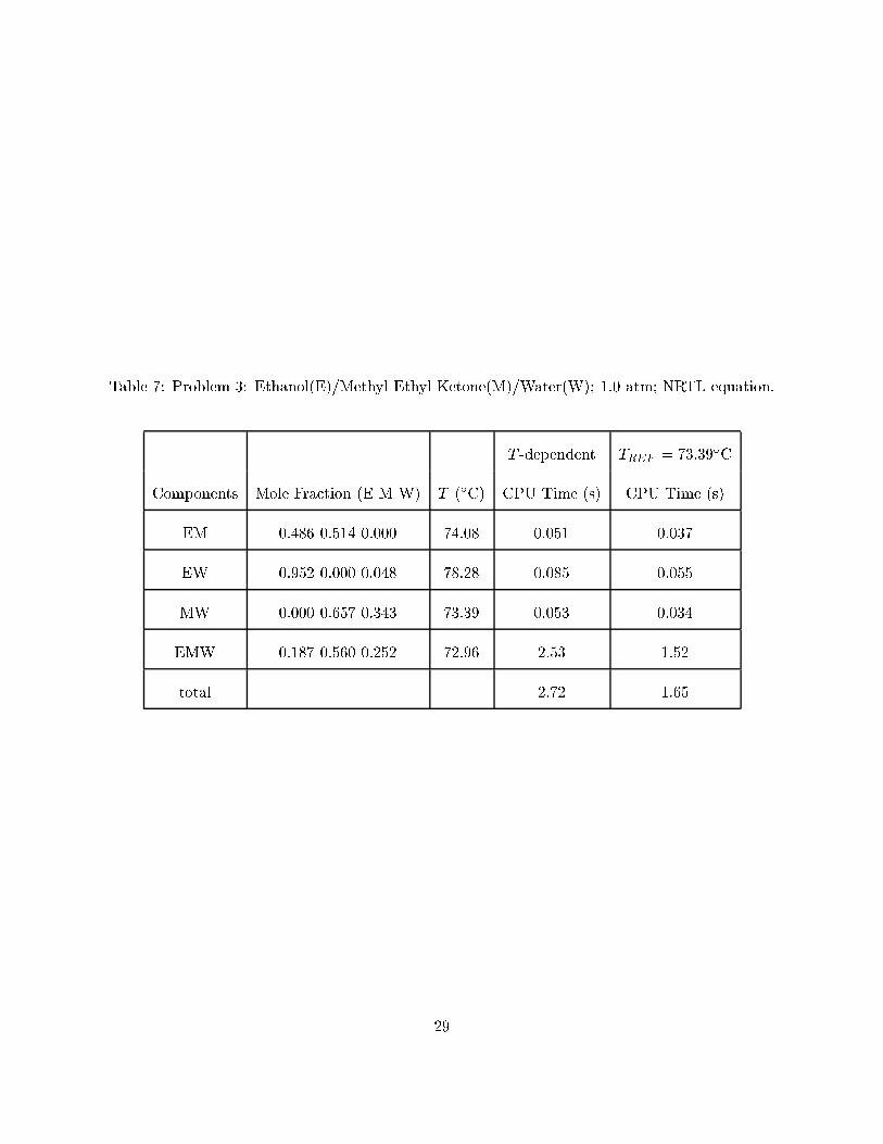
Table 7: Problem 3: Ethanol(E)/Methyl Ethyl Ketone(M)/Water(W); 1.0 atm; NRTL equation.
T -dependent TREF = 73:39ÆC
Components Mole Fraction (E M W) T (ÆC) CPU Time (s) CPU Time (s)
EM 0.486 0.514 0.000 74.08 0.051 0.037
EW 0.952 0.000 0.048 78.28 0.085 0.055
MW 0.000 0.657 0.343 73.39 0.053 0.034
EMW 0.187 0.560 0.252 72.96 2.53 1.52
total 2.72 1.65
29
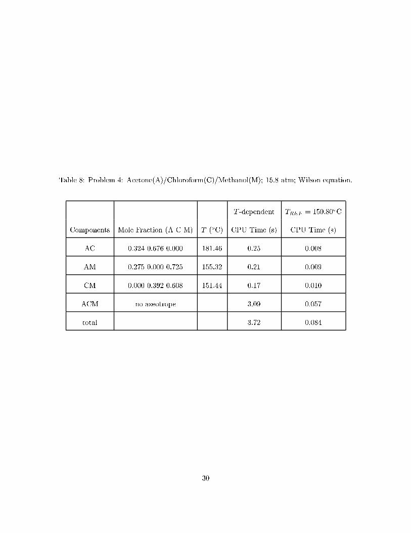
Table 8: Problem 4: Acetone(A)/Chloroform(C)/Methanol(M); 15.8 atm; Wilson equation.
T -dependent TREF = 150:80ÆC
Components Mole Fraction (A C M) T (ÆC) CPU Time (s) CPU Time (s)
AC 0.324 0.676 0.000 181.46 0.25 0.008
AM 0.275 0.000 0.725 155.32 0.21 0.009
CM 0.000 0.392 0.608 151.44 0.17 0.010
ACM no azeotrope 3.09 0.057
total 3.72 0.084
30
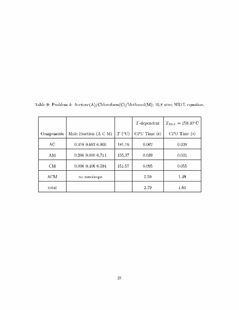
Table 9: Problem 4: Acetone(A)/Chloroform(C)/Methanol(M); 15.8 atm; NRTL equation.
T -dependent TREF = 150:40ÆC
Components Mole Fraction (A C M) T (ÆC) CPU Time (s) CPU Time (s)
AC 0.318 0.682 0.000 181.16 0.062 0.038
AM 0.286 0.000 0.714 155.37 0.039 0.031
CM 0.000 0.406 0.594 151.57 0.095 0.055
ACM no azeotrope 2.59 1.49
total 2.79 1.61
31
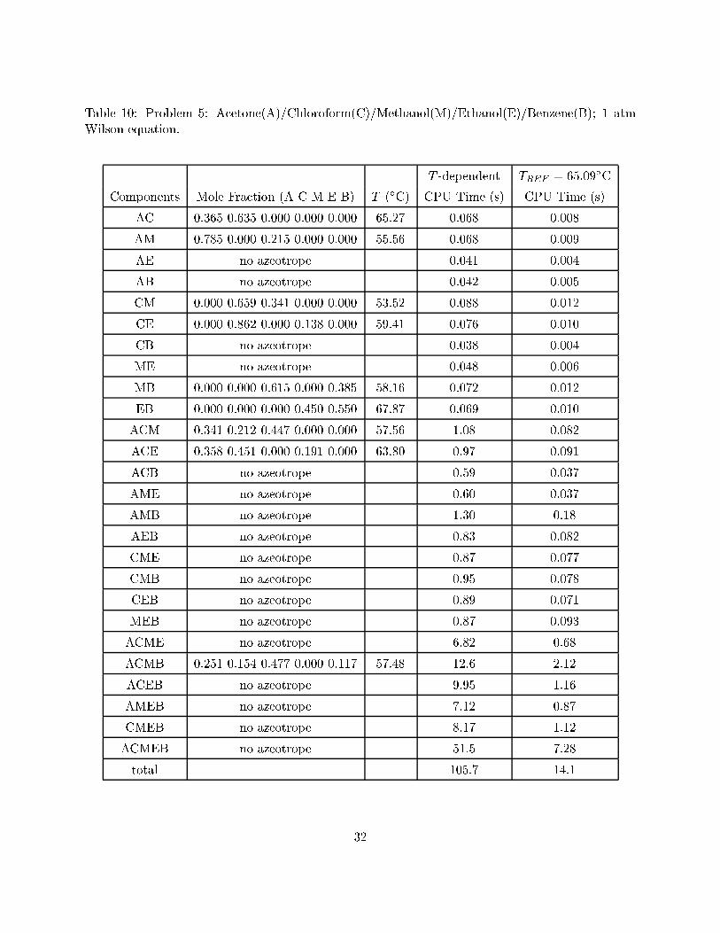
Table 10: Problem 5: Acetone(A)/Chloroform(C)/Methanol(M)/Ethanol(E)/Benzene(B); 1 atmWilson equation.
T -dependent TREF = 65:09ÆC
Components Mole Fraction (A C M E B) T (ÆC) CPU Time (s) CPU Time (s)
AC 0.365 0.635 0.000 0.000 0.000 65.27 0.068 0.008
AM 0.785 0.000 0.215 0.000 0.000 55.56 0.068 0.009
AE no azeotrope 0.041 0.004
AB no azeotrope 0.042 0.005
CM 0.000 0.659 0.341 0.000 0.000 53.52 0.088 0.012
CE 0.000 0.862 0.000 0.138 0.000 59.41 0.076 0.010
CB no azeotrope 0.038 0.004
ME no azeotrope 0.048 0.006
MB 0.000 0.000 0.615 0.000 0.385 58.16 0.072 0.012
EB 0.000 0.000 0.000 0.450 0.550 67.87 0.069 0.010
ACM 0.341 0.212 0.447 0.000 0.000 57.56 1.08 0.082
ACE 0.358 0.451 0.000 0.191 0.000 63.80 0.97 0.091
ACB no azeotrope 0.59 0.037
AME no azeotrope 0.60 0.037
AMB no azeotrope 1.30 0.18
AEB no azeotrope 0.83 0.082
CME no azeotrope 0.87 0.077
CMB no azeotrope 0.95 0.078
CEB no azeotrope 0.89 0.071
MEB no azeotrope 0.87 0.093
ACME no azeotrope 6.82 0.68
ACMB 0.251 0.154 0.477 0.000 0.117 57.48 12.6 2.12
ACEB no azeotrope 9.95 1.16
AMEB no azeotrope 7.12 0.87
CMEB no azeotrope 8.17 1.12
ACMEB no azeotrope 51.5 7.28
total 105.7 14.1
32
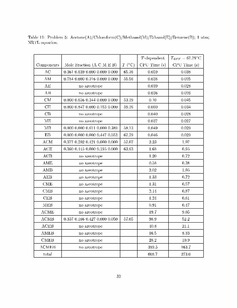
Table 11: Problem 5: Acetone(A)/Chloroform(C)/Methanol(M)/Ethanol(E)/Benzene(B); 1 atm;NRTL equation.
T -dependent TREF = 67:79ÆC
Components Mole Fraction (A C M E B) T (ÆC) CPU Time (s) CPU Time (s)
AC 0.361 0.639 0.000 0.000 0.000 65.26 0.059 0.038
AM 0.784 0.000 0.216 0.000 0.000 55.56 0.038 0.025
AE no azeotrope 0.039 0.028
AB no azeotrope 0.036 0.026
CM 0.000 0.656 0.344 0.000 0.000 53.29 0.10 0.045
CE 0.000 0.847 0.000 0.153 0.000 59.26 0.060 0.034
CB no azeotrope 0.040 0.028
ME no azeotrope 0.037 0.027
MB 0.000 0.000 0.611 0.000 0.389 58.13 0.049 0.029
EB 0.000 0.000 0.000 0.447 0.553 67.79 0.046 0.029
ACM 0.377 0.202 0.421 0.000 0.000 57.07 2.23 1.07
ACE 0.360 0.445 0.000 0.195 0.000 63.63 1.68 0.95
ACB no azeotrope 1.20 0.72
AME no azeotrope 0.58 0.38
AMB no azeotrope 2.02 1.05
AEB no azeotrope 1.33 0.72
CME no azeotrope 1.31 0.57
CMB no azeotrope 2.14 0.87
CEB no azeotrope 1.24 0.61
MEB no azeotrope 0.91 0.47
ACME no azeotrope 19.7 9.05
ACMB 0.357 0.166 0.427 0.000 0.050 57.05 98.9 52.2
ACEB no azeotrope 40.8 21.1
AMEB no azeotrope 16.5 8.33
CMEB no azeotrope 28.2 10.9
ACMEB no azeotrope 389.5 163.7
total 608.7 273.0
33
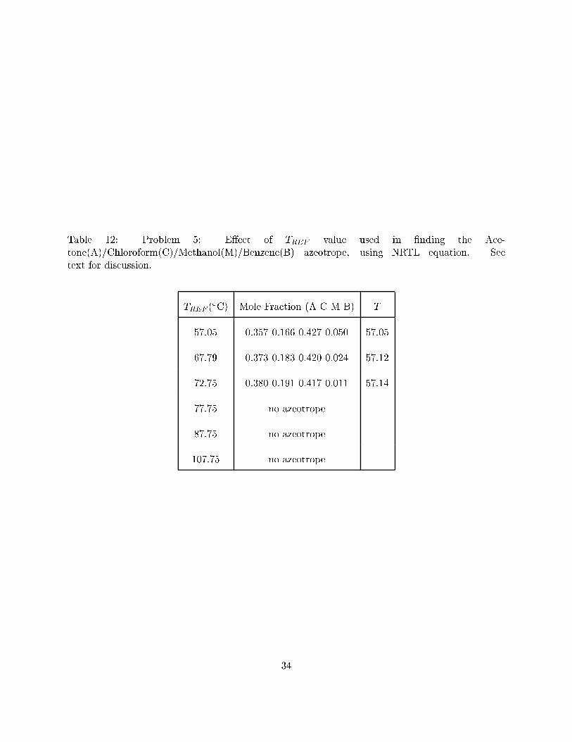
Table 12: Problem 5: E�ect of TREF value used in �nding the Ace-tone(A)/Chloroform(C)/Methanol(M)/Benzene(B) azeotrope, using NRTL equation. Seetext for discussion.
TREF (ÆC) Mole Fraction (A C M B) T
57.05 0.357 0.166 0.427 0.050 57.05
67.79 0.373 0.183 0.420 0.024 57.12
72.75 0.380 0.191 0.417 0.011 57.14
77.75 no azeotrope
87.75 no azeotrope
107.75 no azeotrope
34
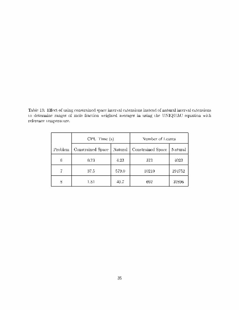
Table 13: E�ect of using constrained space interval extensions instead of natural interval extensionsto determine ranges of mole fraction weighted averages in using the UNIQUAC equation withreference temperature.
CPU Time (s) Number of Leaves
Problem Constrained Space Natural Constrained Space Natural
6 0.73 4.23 373 4023
7 37.5 579.0 10210 294752
8 1.81 40.7 692 32896
35
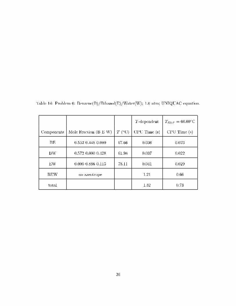
Table 14: Problem 6: Benzene(B)/Ethanol(E)/Water(W); 1.0 atm; UNIQUAC equation.
T -dependent TREF = 60:00ÆC
Components Mole Fraction (B E W) T (ÆC) CPU Time (s) CPU Time (s)
BE 0.552 0.448 0.000 67.66 0.036 0.023
BW 0.572 0.000 0.428 61.98 0.037 0.022
EW 0.000 0.886 0.115 78.11 0.041 0.029
BEW no azeotrope 1.21 0.66
total 1.32 0.73
36
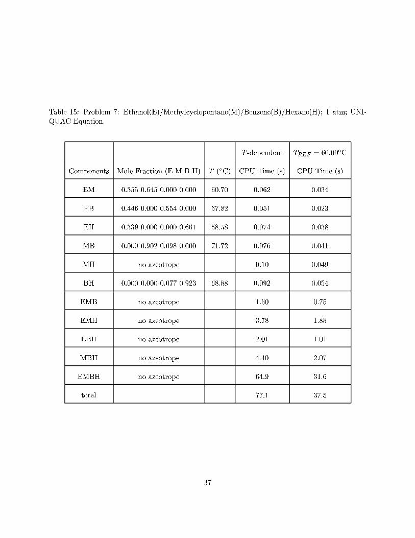
Table 15: Problem 7: Ethanol(E)/Methylcyclopentane(M)/Benzene(B)/Hexane(H); 1 atm; UNI-QUAC Equation.
T -dependent TREF = 60:00ÆC
Components Mole Fraction (E M B H) T (ÆC) CPU Time (s) CPU Time (s)
EM 0.355 0.645 0.000 0.000 60.70 0.062 0.034
EB 0.446 0.000 0.554 0.000 67.82 0.051 0.023
EH 0.339 0.000 0.000 0.661 58.58 0.074 0.038
MB 0.000 0.902 0.098 0.000 71.72 0.076 0.041
MH no azeotrope 0.10 0.049
BH 0.000 0.000 0.077 0.923 68.88 0.092 0.054
EMB no azeotrope 1.60 0.75
EMH no azeotrope 3.78 1.88
EBH no azeotrope 2.01 1.01
MBH no azeotrope 4.40 2.07
EMBH no azeotrope 64.9 31.6
total 77.1 37.5
37
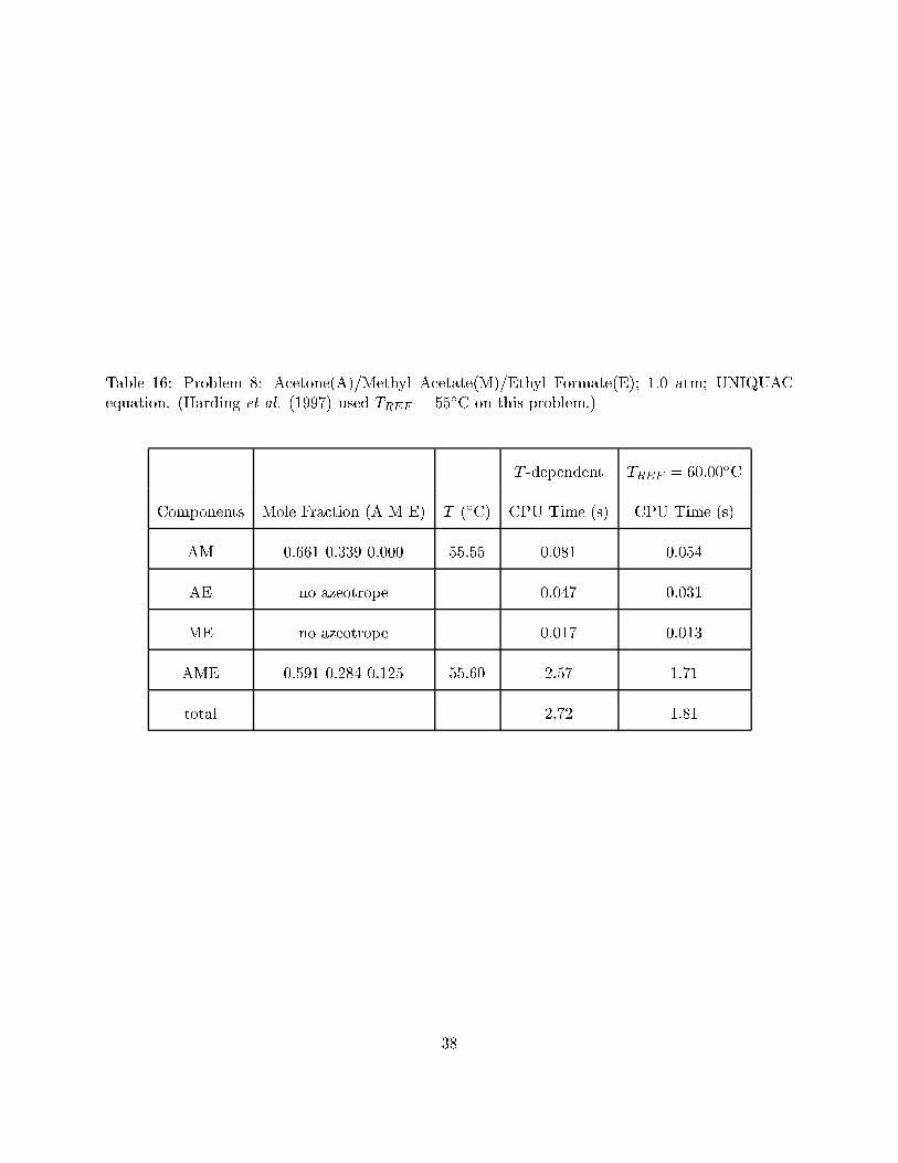
Table 16: Problem 8: Acetone(A)/Methyl Acetate(M)/Ethyl Formate(E); 1.0 atm; UNIQUACequation. (Harding et al. (1997) used TREF = 55ÆC on this problem.)
T -dependent TREF = 60:00ÆC
Components Mole Fraction (A M E) T (ÆC) CPU Time (s) CPU Time (s)
AM 0.661 0.339 0.000 55.55 0.081 0.054
AE no azeotrope 0.047 0.031
ME no azeotrope 0.017 0.013
AME 0.591 0.284 0.125 55.60 2.57 1.71
total 2.72 1.81
38
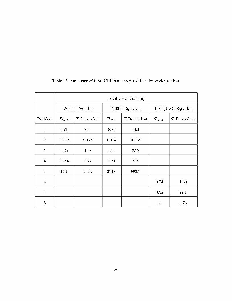
Table 17: Summary of total CPU time required to solve each problem.
Total CPU Time (s)
Wilson Equation NRTL Equation UNIQUAC Equation
Problem TREF T -Dependent TREF T -Dependent TREF T -Dependent
1 0.71 7.30 8.80 14.3
2 0.029 0.145 0.134 0.215
3 0.25 1.68 1.65 2.72
4 0.084 3.72 1.61 2.79
5 14.1 105.7 273.0 608.7
6 0.73 1.32
7 37.5 77.1
8 1.81 2.72
39
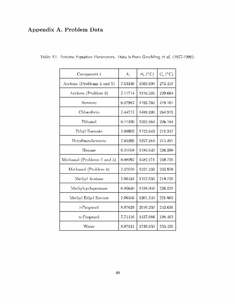
Appendix A. Problem Data
Table A1. Antoine Equation Parameters. Data is from Gmehling et al. (1977-1990).
Component i Ai Bi (ÆC) Ci (
ÆC)
Acetone (Problems 4 and 5) 7.63130 1566.690 273.419
Acetone (Problem 8) 7.11714 1210.595 229.664
Benzene 6.87987 1196.760 219.161
Chloroform 7.44777 1488.990 264.915
Ethanol 8.11220 1592.864 226.184
Ethyl Formate 7.00902 1123.943 218.247
Hexa uorobenzene 7.03295 1227.984 215.491
Hexane 6.91058 1189.640 226.280
Methanol (Problems 1 and 5) 8.08097 1582.271 239.726
Methanol (Problem 4) 7.97010 1521.230 233.970
Methyl Acetate 7.06524 1157.630 219.726
Methylcyclopentane 6.86640 1188.050 226.276
Methyl Ethyl Ketone 7.06356 1261.340 221.969
i-Propanol 8.87829 2010.330 252.636
n-Propanol 7.74416 1437.686 198.463
Water 8.07131 1730.630 233.426
40
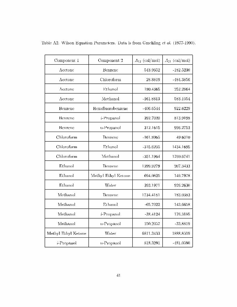
Table A2. Wilson Equation Parameters. Data is from Gmehling et al. (1977-1990).
Component 1 Component 2 A12 (cal/mol) A21 (cal/mol)
Acetone Benzene 543.9352 -182.5230
Acetone Chloroform 28.8819 -484.3856
Acetone Ethanol 180.4365 252.2864
Acetone Methanol -161.8813 583.1054
Benzene Hexa uorobenzene -406.6544 922.6229
Benzene i-Propanol 392.7020 813.9198
Benzene n-Propanol 312.1615 996.2753
Chloroform Benzene -161.8065 49.6010
Chloroform Ethanol -315.6205 1434.1695
Chloroform Methanol -351.1964 1760.6741
Ethanol Benzene 1399.9279 207.3433
Ethanol Methyl Ethyl Ketone 694.0825 -149.7978
Ethanol Water 393.1971 926.2630
Methanol Benzene 1734.4181 183.0383
Methanol Ethanol -65.7022 143.6658
Methanol i-Propanol -38.4124 176.3185
Methanol n-Propanol 150.2057 -33.8819
Methyl Ethyl Ketone Water 6811.3433 1888.8509
i-Propanol n-Propanol 818.3291 -481.0590
41
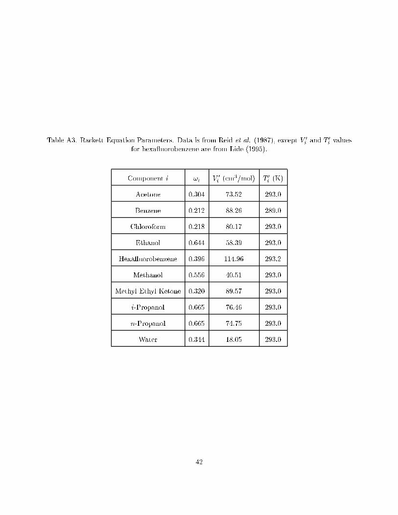
Table A3. Rackett Equation Parameters. Data is from Reid et al. (1987), except V 0
i and T 0
i valuesfor hexa uorobenzene are from Lide (1995).
Component i !i V 0
i (cm3/mol) T 0
i (K)
Acetone 0.304 73.52 293.0
Benzene 0.212 88.26 289.0
Chloroform 0.218 80.17 293.0
Ethanol 0.644 58.39 293.0
Hexa uorobenzene 0.396 114.96 293.2
Methanol 0.556 40.51 293.0
Methyl Ethyl Ketone 0.320 89.57 293.0
i-Propanol 0.665 76.46 293.0
n-Propanol 0.665 74.75 293.0
Water 0.344 18.05 293.0
42
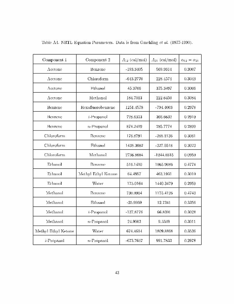
Table A4. NRTL Equation Parameters. Data is from Gmehling et al. (1977-1990).
Component 1 Component 2 A12 (cal/mol) A21 (cal/mol) �12 = �21
Acetone Benzene -193.3405 569.9314 0.3007
Acetone Chloroform -643.2770 228.4574 0.3043
Acetone Ethanol 45.3706 375.3497 0.3006
Acetone Methanol 184.7013 222.6450 0.3084
Benzene Hexa uorobenzene 1251.4578 -794.4003 0.2978
Benzene i-Propanol 728.6353 366.6632 0.2910
Benzene n-Propanol 874.2419 285.7774 0.2899
Chloroform Benzene 176.8791 -288.2136 0.3061
Chloroform Ethanol 1438.3602 -327.5518 0.3023
Chloroform Methanol 2736.8604 -1244.0315 0.0950
Ethanol Benzene 516.1410 1065.9086 0.4774
Ethanol Methyl Ethyl Ketone 64.4957 463.1931 0.3010
Ethanol Water -175.0164 1440.3479 0.2959
Methanol Benzene 730.0904 1175.4126 0.4743
Methanol Ethanol -25.9969 12.7341 0.3356
Methanol i-Propanol -137.8776 66.8301 0.3028
Methanol n-Propanol 24.9003 9.5349 0.3011
Methyl Ethyl Ketone Water 674.4614 1809.8868 0.3536
i-Propanol n-Propanol -673.7647 991.7833 0.2978
43
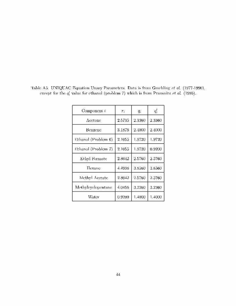
Table A5. UNIQUAC Equation Unary Parameters. Data is from Gmehling et al. (1977-1990),except for the q0i value for ethanol (problem 7) which is from Prausnitz et al. (1986).
Component i ri qi q0i
Acetone 2.5735 2.3360 2.3360
Benzene 3.1878 2.4000 2.4000
Ethanol (Problem 6) 2.1055 1.9720 1.9720
Ethanol (Problem 7) 2.1055 1.9720 0.9200
Ethyl Formate 2.8042 2.5760 2.5760
Hexane 4.4998 3.8560 3.8560
Methyl Acetate 2.8042 2.5760 2.5760
Methylcyclopentane 4.0456 3.2360 3.2360
Water 0.9200 1.4000 1.4000
44
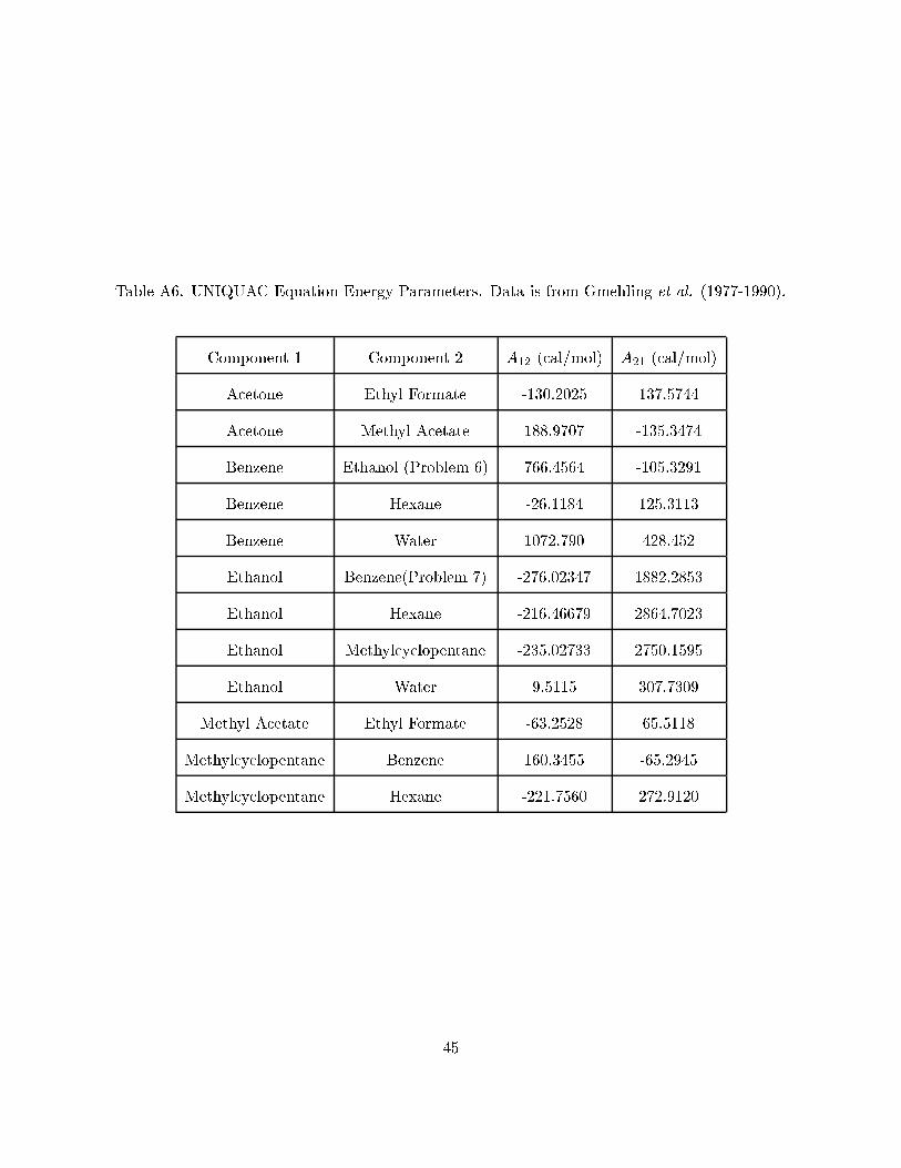
Table A6. UNIQUAC Equation Energy Parameters. Data is from Gmehling et al. (1977-1990).
Component 1 Component 2 A12 (cal/mol) A21 (cal/mol)
Acetone Ethyl Formate -130.2025 137.5744
Acetone Methyl Acetate 188.9707 -135.3474
Benzene Ethanol (Problem 6) 766.4564 -105.3291
Benzene Hexane -26.1184 125.3113
Benzene Water 1072.790 428.452
Ethanol Benzene(Problem 7) -276.02347 1882.2853
Ethanol Hexane -216.46679 2864.7023
Ethanol Methylcyclopentane -235.02733 2750.1595
Ethanol Water 9.5115 307.7309
Methyl Acetate Ethyl Formate -63.2528 65.5118
Methylcyclopentane Benzene 160.3455 -65.2945
Methylcyclopentane Hexane -221.7560 272.9120
45