Embed Size (px)
Citation preview

ABSTRACT
Title of dissertation: CHARGE FORM FACTOR OF
THE NEUTRON THROUGH ~d(~e, e′n)
AT Q2 = 1.0 (GeV/c)2
Nikolai Aleksandrovich Savvinov, Doctor of Philosophy, 2003
Dissertation directed by: Professor James J. Kelly
Department of Physics
Elastic electromagnetic form factors of the nucleon are of fundamental impor-
tance for our understanding of its internal structure. Experiment E93-026 at the
Thomas Jefferson National Accelerator Facility (JLab) determined the electric form
factor of the neutron, GnE, through quasielastic ~d(~e, e′n)p scattering using a longitu-
dinally polarized electron beam and a frozen polarized 15ND3 target. The knocked
out neutrons were detected in a segmented plastic scintillator detector in coinci-
dence with the scattered electrons. The form factor was extracted by comparing
the experimental beam–target asymmetry with full theoretical calculations based
on different values of GnE. The dissertation discusses the experimental setup, data
acquisition and analysis for the Q2 = 1.0 (GeV/c)2 point, and implications of the
experimental results for our understanding of the nucleon electromagnetic structure.
CHARGE FORM FACTOR OF THE NEUTRON
THROUGH ~d(~e, e′n) AT Q2 = 1.0 (GeV/c)2
by
Nikolai Aleksandrovich Savvinov
Dissertation submitted to the Faculty of the Graduate School of theUniversity of Maryland, College Park in partial fulfillment
of the requirements for the degree ofDoctor of Philosophy
2003
Advisory Commmittee:
Professor James J. Kelly, Chair/AdvisorProfessor Xiangdong JiProfessor Elizabeth J. BeiseProfessor Philip G. RoosProfessor Alice C. Mignerey

c© Copyright by
Nikolai Aleksandrovich Savvinov
2003
i

To the memory of my father.
ii
Contents
1 Introduction 1
2 Basic concepts and definitions 5
2.1 Nucleon form factors . . . . . . . . . . . . . . . . . . . . . . . . . . . 5
2.2 Charge and magnetization densities . . . . . . . . . . . . . . . . . . . 9
2.3 Charge radius of the neutron . . . . . . . . . . . . . . . . . . . . . . . 13
3 Previous GnE experiments 15
3.1 Rosenbluth separation . . . . . . . . . . . . . . . . . . . . . . . . . . 15
3.2 Unpolarized elastic e− d scattering . . . . . . . . . . . . . . . . . . . 18
3.3 Hybrid analysis of the elastic e− d data . . . . . . . . . . . . . . . . 22
3.4 Polarized measurements . . . . . . . . . . . . . . . . . . . . . . . . . 23
4 Experimental technique 27
4.1 Polarized scattering from a free nucleon . . . . . . . . . . . . . . . . . 27
4.2 Deuteron target . . . . . . . . . . . . . . . . . . . . . . . . . . . . . . 29
5 Experimental setup 34
iii

5.1 Polarized electron beam . . . . . . . . . . . . . . . . . . . . . . . . . 35
5.1.1 Accelerator . . . . . . . . . . . . . . . . . . . . . . . . . . . . 35
5.1.2 Hall C beamline . . . . . . . . . . . . . . . . . . . . . . . . . . 37
5.1.3 Raster magnets . . . . . . . . . . . . . . . . . . . . . . . . . . 40
5.1.4 Chicane magnets . . . . . . . . . . . . . . . . . . . . . . . . . 41
5.2 Hall C High Momentum Spectrometer . . . . . . . . . . . . . . . . . 41
5.3 Polarized target . . . . . . . . . . . . . . . . . . . . . . . . . . . . . . 44
5.3.1 Magnet . . . . . . . . . . . . . . . . . . . . . . . . . . . . . . 44
5.3.2 Refrigerator . . . . . . . . . . . . . . . . . . . . . . . . . . . . 45
5.3.3 Insert . . . . . . . . . . . . . . . . . . . . . . . . . . . . . . . 47
5.3.4 Microwaves . . . . . . . . . . . . . . . . . . . . . . . . . . . . 47
5.3.5 NMR and data acquisition . . . . . . . . . . . . . . . . . . . . 48
5.3.6 Target material . . . . . . . . . . . . . . . . . . . . . . . . . . 49
5.4 Neutron detector . . . . . . . . . . . . . . . . . . . . . . . . . . . . . 50
5.4.1 Configuration and position . . . . . . . . . . . . . . . . . . . . 51
5.4.2 Gain monitoring . . . . . . . . . . . . . . . . . . . . . . . . . 54
5.4.3 Gain matching . . . . . . . . . . . . . . . . . . . . . . . . . . 55
5.5 Electronics and data acquisition . . . . . . . . . . . . . . . . . . . . . 55
5.5.1 Electronics . . . . . . . . . . . . . . . . . . . . . . . . . . . . . 56
5.5.2 Triggers and events . . . . . . . . . . . . . . . . . . . . . . . . 60
6 Analysis software 65
iv
6.1 Overview . . . . . . . . . . . . . . . . . . . . . . . . . . . . . . . . . . 65
6.2 Syncfilter . . . . . . . . . . . . . . . . . . . . . . . . . . . . . . . . . 67
6.3 Hall C replay engine . . . . . . . . . . . . . . . . . . . . . . . . . . . 69
6.3.1 HMS event reconstruction . . . . . . . . . . . . . . . . . . . . 70
6.3.2 Neutron detector event reconstruction . . . . . . . . . . . . . 73
6.3.3 Kinematic calculations . . . . . . . . . . . . . . . . . . . . . . 78
6.4 Inclusive simulations . . . . . . . . . . . . . . . . . . . . . . . . . . . 81
6.4.1 Cross-section model . . . . . . . . . . . . . . . . . . . . . . . . 81
6.4.2 QFS parameters . . . . . . . . . . . . . . . . . . . . . . . . . . 85
6.4.3 Deuterium cross sections . . . . . . . . . . . . . . . . . . . . . 85
6.4.4 Radiative effects . . . . . . . . . . . . . . . . . . . . . . . . . 87
6.4.5 Acceptance effects . . . . . . . . . . . . . . . . . . . . . . . . 92
6.4.6 Composite target models . . . . . . . . . . . . . . . . . . . . . 94
6.4.7 Comparison of simulation results to experimental data . . . . 95
6.5 Coincidence Monte Carlo simulations . . . . . . . . . . . . . . . . . . 96
6.5.1 Basics of MCEEP . . . . . . . . . . . . . . . . . . . . . . . . . 97
6.5.2 Customization of MCEEP . . . . . . . . . . . . . . . . . . . . 101
6.5.3 Output and results . . . . . . . . . . . . . . . . . . . . . . . . 104
7 Data analysis 106
7.1 Data replay . . . . . . . . . . . . . . . . . . . . . . . . . . . . . . . . 106
7.1.1 Runs selection . . . . . . . . . . . . . . . . . . . . . . . . . . . 107
v
7.1.2 Detector calibrations . . . . . . . . . . . . . . . . . . . . . . . 108
7.1.3 Replay procedure . . . . . . . . . . . . . . . . . . . . . . . . . 109
7.2 Cut optimization . . . . . . . . . . . . . . . . . . . . . . . . . . . . . 110
7.3 Target polarization . . . . . . . . . . . . . . . . . . . . . . . . . . . . 113
7.3.1 Baseline subtraction . . . . . . . . . . . . . . . . . . . . . . . 113
7.3.2 TE constants . . . . . . . . . . . . . . . . . . . . . . . . . . . 115
7.4 Beam polarization . . . . . . . . . . . . . . . . . . . . . . . . . . . . . 116
7.4.1 Hall A current leakage . . . . . . . . . . . . . . . . . . . . . . 117
7.4.2 Results . . . . . . . . . . . . . . . . . . . . . . . . . . . . . . . 118
7.5 Packing fraction . . . . . . . . . . . . . . . . . . . . . . . . . . . . . . 120
7.5.1 Method of determination . . . . . . . . . . . . . . . . . . . . . 120
7.5.2 Event selection . . . . . . . . . . . . . . . . . . . . . . . . . . 121
7.5.3 Procedure and results . . . . . . . . . . . . . . . . . . . . . . . 122
7.6 Dilution factor . . . . . . . . . . . . . . . . . . . . . . . . . . . . . . 124
7.6.1 Pion contamination . . . . . . . . . . . . . . . . . . . . . . . . 126
7.6.2 Misorientation of the 4K shield . . . . . . . . . . . . . . . . . 126
7.6.3 Stick 3 rotation . . . . . . . . . . . . . . . . . . . . . . . . . . 127
7.6.4 Results . . . . . . . . . . . . . . . . . . . . . . . . . . . . . . . 131
7.7 Corrections . . . . . . . . . . . . . . . . . . . . . . . . . . . . . . . . 132
7.7.1 Radiative corrections . . . . . . . . . . . . . . . . . . . . . . . 132
7.7.2 Paddle inefficiency . . . . . . . . . . . . . . . . . . . . . . . . 133
vi

7.7.3 Electronics deadtime . . . . . . . . . . . . . . . . . . . . . . . 135
7.7.4 Accidental background subtraction . . . . . . . . . . . . . . . 136
7.7.5 Multi-step reactions contamination . . . . . . . . . . . . . . . 139
7.8 Results . . . . . . . . . . . . . . . . . . . . . . . . . . . . . . . . . . . 141
7.8.1 Extraction of GnE . . . . . . . . . . . . . . . . . . . . . . . . . 141
7.8.2 Kinematic uncertainties . . . . . . . . . . . . . . . . . . . . . 146
7.8.3 Other experimental uncertainties . . . . . . . . . . . . . . . . 146
7.8.4 Reaction mechanism dependence . . . . . . . . . . . . . . . . 148
7.8.5 Parametrization of GnE . . . . . . . . . . . . . . . . . . . . . . 149
8 Theoretical predictions of GnE 151
8.1 Asymptotic behavior . . . . . . . . . . . . . . . . . . . . . . . . . . . 151
8.1.1 Dimensional scaling laws . . . . . . . . . . . . . . . . . . . . . 151
8.1.2 Perturbative QCD calculations. . . . . . . . . . . . . . . . . . 153
8.1.3 Comparison with experiment . . . . . . . . . . . . . . . . . . . 157
8.2 Dispersion relations . . . . . . . . . . . . . . . . . . . . . . . . . . . . 162
8.3 Vector Meson Dominance . . . . . . . . . . . . . . . . . . . . . . . . 163
8.4 Quark models . . . . . . . . . . . . . . . . . . . . . . . . . . . . . . . 166
8.4.1 Nonrelativistic quark models . . . . . . . . . . . . . . . . . . . 166
8.4.2 Relativistic constituent quark models . . . . . . . . . . . . . . 168
8.5 Diquark model . . . . . . . . . . . . . . . . . . . . . . . . . . . . . . 172
8.6 Soliton model . . . . . . . . . . . . . . . . . . . . . . . . . . . . . . . 177
vii
8.7 Overview . . . . . . . . . . . . . . . . . . . . . . . . . . . . . . . . . . 179
9 Discussion 183
10 Summary and outlook 188
A Principles of operation of the E93026 polarized target 190
A.1 Dynamic nuclear polarization . . . . . . . . . . . . . . . . . . . . . . 190
A.2 NMR polarization measurement . . . . . . . . . . . . . . . . . . . . . 192
B Measuring beam polarization with the Hall C Møller polarimeter 196
Bibliography 198
viii
List of Figures
2.1 One-photon-exchange diagram for electron-nucleon scattering. . . . . 6
2.2 Nucleon charge and magnetization densities. . . . . . . . . . . . . . . . 11
3.1 Longitudinal-transverse separation. . . . . . . . . . . . . . . . . . . . . 16
3.2 Best Rosenbluth data for GnE. . . . . . . . . . . . . . . . . . . . . . . . 18
3.3 Elastic measurements of GnE . . . . . . . . . . . . . . . . . . . . . . . . 20
3.4 Sick and Schiavilla’s extraction of Gn. . . . . . . . . . . . . . . . . . . 23
3.5 Polarized measurements of GnE . . . . . . . . . . . . . . . . . . . . . . 26
4.1 Polarized electron-nucleon scattering. . . . . . . . . . . . . . . . . . . 29
4.2 Meson exchange currents . . . . . . . . . . . . . . . . . . . . . . . . . . 31
4.3 Isobar currents . . . . . . . . . . . . . . . . . . . . . . . . . . . . . . . 31
4.4 The vector beam-target asymmetry AVed . . . . . . . . . . . . . . . . . 33
5.1 Schematic view of the JLab accelerator . . . . . . . . . . . . . . . . . . 36
5.2 Hall C beamline elements . . . . . . . . . . . . . . . . . . . . . . . . . 38
5.3 Layout of the Hall C Møller polarimeter . . . . . . . . . . . . . . . . . 39
5.4 Rastered beam . . . . . . . . . . . . . . . . . . . . . . . . . . . . . . . 41
ix
5.5 Chicane magnets. . . . . . . . . . . . . . . . . . . . . . . . . . . . . . . 42
5.6 Hall C High Momentum Spectrometer . . . . . . . . . . . . . . . . . . 43
5.7 Main components of the UVa polarized target. . . . . . . . . . . . . . . 45
5.8 Target cryostat and magnet. . . . . . . . . . . . . . . . . . . . . . . . . 46
5.9 Target ladder carrying target cells. . . . . . . . . . . . . . . . . . . . . 48
5.10 The neutron detector. . . . . . . . . . . . . . . . . . . . . . . . . . . . 52
5.11 HMS trigger electronics. . . . . . . . . . . . . . . . . . . . . . . . . . . 57
5.12 Neutron detector electronics. . . . . . . . . . . . . . . . . . . . . . . . 58
5.13 Laser trigger . . . . . . . . . . . . . . . . . . . . . . . . . . . . . . . . 59
5.14 Helicity scaler electronics. . . . . . . . . . . . . . . . . . . . . . . . . . 60
5.15 Trigger setup. . . . . . . . . . . . . . . . . . . . . . . . . . . . . . . . . 63
6.1 Data analysis software. . . . . . . . . . . . . . . . . . . . . . . . . . . . 66
6.2 A proton event in the neutron detector . . . . . . . . . . . . . . . . . . 75
6.3 QFS versus NE4 data for transverse scattering . . . . . . . . . . . . . . 88
6.4 Comparison between SLAC NE3 data and simulations . . . . . . . . . 91
6.5 HMS momentum acceptance. . . . . . . . . . . . . . . . . . . . . . . . 93
6.6 HMS acceptance . . . . . . . . . . . . . . . . . . . . . . . . . . . . . . 93
6.7 Comparison between single-arm data and simulation results. . . . . . . 96
6.8 Coincidence Monte Carlo compared to data . . . . . . . . . . . . . . . 105
7.1 Figure of merit for different kinematic cuts . . . . . . . . . . . . . . . . 111
7.2 NMR signal on different stages of the offline analysis. . . . . . . . . . 114
x

7.3 TE calibration constants for various groups . . . . . . . . . . . . . . . 115
7.4 Results of Møller measurements and their parameterizations. . . . . . . 119
7.5 Packing fraction for stick 4 . . . . . . . . . . . . . . . . . . . . . . . . 123
7.6 The ZBEAM distribution . . . . . . . . . . . . . . . . . . . . . . . . . . 128
7.7 A top view of the cup inside the 4K shield . . . . . . . . . . . . . . . . 129
7.8 Target insert rotation . . . . . . . . . . . . . . . . . . . . . . . . . . . 130
7.9 The number of HMS events as a function of the gate width . . . . . . . 136
7.10 Hits meantime distribution . . . . . . . . . . . . . . . . . . . . . . . . 137
7.11 Relative track excess versus the background level . . . . . . . . . . . . 139
7.12 The GnE extraction plot. . . . . . . . . . . . . . . . . . . . . . . . . . . 143
7.13 Statistical properties of neutron asymmetries . . . . . . . . . . . . . . 144
7.14 Proton asymmetries . . . . . . . . . . . . . . . . . . . . . . . . . . . . 145
7.15 Results of JLab E93-026 compared with other experimental data. . . . 150
8.1 Elastic e−N scattering amplitude at high Q2. . . . . . . . . . . . . . 152
8.2 A two-gluon exchange hard scattering diagram for F p2 . . . . . . . . . . 156
8.3 Asymptotic behavior of the proton magnetic form factor . . . . . . . . 158
8.4 Recent data on the proton form factor ratio. . . . . . . . . . . . . . . . 159
8.5 Magnetic form factors of the nucleon . . . . . . . . . . . . . . . . . . . 181
8.6 The GE/GM ratio for the proton. . . . . . . . . . . . . . . . . . . . . 182
8.7 The electric form factor of the neutron . . . . . . . . . . . . . . . . . . 182
9.1 Charge and magnetization densities of the neutron . . . . . . . . . . . 187
xi

A.1 The effect of spin-spin interaction on levels and states of an electron-
nucleon system in an external magnetic field . . . . . . . . . . . . . . . 193
A.2 Positive and negative polarization enhancement . . . . . . . . . . . . . 194
xii
Chapter 1
Introduction
“What does matter consist of?” is one of the most ancient and fundamental ques-
tions. It is more than just a mere curiosity; one hopes that the myriad phenomena
around us and thousands of empirical laws governing them can be reduced to a
few basic constituents and the rules of their interaction. This was the basis of the
determinism of the XVII century – an attitude that claimed that everything was
calculable and predictable. The XX century, with establishing of probabilistic na-
ture of the microscopic world, with discovery of deterministic chaos, and with the
realization of the enormous computational difficulties that may arise in application
of simple theories to practice, has shattered this optimism. Still, there is no doubt
that understanding the primary constituents of matter will shed light on the most
exciting and challenging puzzles of the modern science.
During the last two centuries science has made a lot of progress in this di-
rection. It has been known for more than a century that ordinary matter is made
of atoms. It has also been known since Rutherford’s famous experiment in 1911
1

that an atom consists of a heavy nucleus surrounded by light electrons. Further
experiments that followed in 1920-s and 1930-s revealed that nuclei, in their turn,
are comprised of protons and neutrons, two particles similar in mass and strong
interaction properties, but differing in electric charge and magnetic moment. And
finally, vast experimental evidence starting with the hard scattering experiments of
1960-s has convinced the scientific community that nucleons (as well as all other
strongly interacting particles) consist of point-like quarks interacting by means of
gluon exchange, even though quarks have never been observed directly.
The answer to the next important question, how matter is made, i.e. how
the elementary constituents interact strongly with each other, is to be given by
quantum chromodynamics (QCD). Even though the QCD Lagrangian is known, it
is very hard to solve it because of the extreme nonlinearity of the problem1. The
only method which allows model-independent QCD calculations to be made from
first principles, so-called lattice QCD, has only recently produced promising results.
A more practical approach to the problems of physics of strong interactions is to
construct models that emphasize the most important aspects of QCD, and to test
them by confronting them with the data.
Much about the electromagnetic structure of the nucleons can be learned by
probing them with virtual photons in electron-nucleon scattering. In particular, it
1At high momentum transfers the asymptotic freedom of QCD (i.e. weakening of the stronginteraction due to screening of the color charge at Q2 → ∞) allows to solve it perturbatively.These results are often accurate only to logarithmic corrections and it is not always clear at whatQ2 the asymptotic behavior sets in.
2

gives access to electromagnetic form factors of the nucleon (EMFFN). These form
factors not only provide a testing ground for QCD-inspired models, but also are
important in many areas of particle and nuclear physics, including nuclear charge
radii, parity-violating experiments, and many others.
Of the four elastic form factors of the nucleon, the charge form factor of the
neutron GnE is perhaps the most intriguing one. If the SU(6) spin-flavor symmetry of
QCD were exact, this quantity would vanish at all momentum transfers. Therefore
the non-zero experimental values of GnE are a clear signature of dynamical SU(6)-
breaking effects2, and thus by studying GnE we can achieve a better understanding
of spin-dependent interactions between the quarks.
At the same time, GnE has proven to be the most elusive form factor to mea-
sure. The reason for that is fourfold: first, since there is no free neutron target,
experiments on neutron form factors inevitably involve model-dependent nuclear
corrections. Second, since neutrons do not carry electric charge, they are much
harder to detect than the protons. Third, time-of-flight momentum measurements
for the neutron are usually less accurate the magnetic spectrometer measurements
for the proton. Fourth, due to its small magnitude, the electric form factor is com-
pletely overshadowed by a much larger contribution from the magnetic form factor
in the cross section, at least at experimentally accessible Q2.
Therefore, the large theoretical demand for the accurate information on GnE
2Recently it has been shown [1] that kinematic SU(6) breaking via Melosh rotations can beimportant, too. However, the value of Gn
E cannot be explained by relativistic effects alone.
3

(especially at high Q2) is far from being satisfied. A number of new-generation
experiments on GnE employing spin degrees of freedom are currently underway, re-
cently completed, or expected to run in near future. These experiments, being less
susceptible to the model dependence and various systematic errors than traditional
cross-section measurements, are bringing our knowledge of GnE to a new level. The
experiment described here is a part of this experimental program.
The rest of the dissertation is organized as follows: in the next chapter (Chap-
ter 2) we will present the definition and interpretation of the elastic form factors. In
Chapter 3 we will discuss previous measurements of the neutron charge form factor.
As the last preparation for the discussion of the experiment, we introduce the basics
of polarized electron-deuteron scattering in Chapter 4. Chapters 5-10 deal with the
experimental details; Chapter 5 describes the experimental setup, Chapter 6 de-
scribes the software used in the data analysis, and Chapter 7 is devoted to the data
analysis itself and its results. In Chapter 8 we will review various theoretical models
and calculations on the subject. Chapter 9 discusses the implications of our and
other recent experimental results for the electromagnetic structure of the nucleon.
The summary and the outlook are given in the Chapter 10.
4

Chapter 2
Basic concepts and definitions
2.1 Nucleon form factors
Let us consider electron-nucleon scattering. Since the electromagnetic interaction
is relatively weak (the electromagnetic coupling constant α¿ 1), it can be treated
perturbatively. In terms of Feynman diagrams, rapid convergence of the perturba-
tion series means that the contribution of the one-virtual-photon-exchange diagram
(see Figure 2.1) dominates1. In this approximation, the invariant matrix element
becomes [2]
M =4πα
Q2〈~kfλf |jeµ|~kiλi〉〈~pfsf |jNµ |~pisi〉 (2.1)
where α = 1/137 is the fine structure constant, Q2 = −qµqµ is the four-momentum
transfer squared, ki,f and λi,f are the momentum and helicity of the initial and
the final state of the electron, pi,f and si,f denote the initial and final spin and
1The discrepancy between GpE/G
pM measurements via Rosenbluth separation and with recoil
polarimetry have caused some concern with about validity of this approximation. See also thefootnote on page 157.
5

Figure 2.1: One-photon-exchange diagram for electron-nucleon scattering.
momentum of the struck nucleon, and jAµ is the current operator for the particle
A = e,N. It is convenient to introduce lepton and nucleon response tensors as
ηAµν = NA〈jAµ jA†ν 〉 (2.2)
where NA is a constant normalization factor (2m2e for the electron and 1/(2m2
N) for
the nucleon) and angle brackets denote averaging over the initial states and summing
over the final states.
For the electron the unpolarized current is given by
〈~kfλf |jeµ|~kiλi〉 = ufγµui. (2.3)
Using (2.3), spinor normalization relations and trace theorems it is straightforward
6
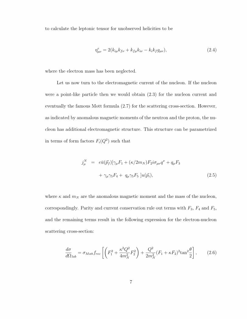
to calculate the leptonic tensor for unobserved helicities to be
ηeµν = 2(kiµkfν + kfµkiν − kikfgµν), (2.4)
where the electron mass has been neglected.
Let us now turn to the electromagnetic current of the nucleon. If the nucleon
were a point-like particle then we would obtain (2.3) for the nucleon current and
eventually the famous Mott formula (2.7) for the scattering cross-section. However,
as indicated by anomalous magnetic moments of the neutron and the proton, the nu-
cleon has additional electromagnetic structure. This structure can be parametrized
in terms of form factors Fi(Q2) such that
jNµ = eu(~pf )[γµF1 + (κ/2mN)F2iσµνqν + qµF3
+ γµγ5F4 + qµγ5F5 ]u(~pi), (2.5)
where κ and mN are the anomalous magnetic moment and the mass of the nucleon,
correspondingly. Parity and current conservation rule out terms with F3, F4 and F5,
and the remaining terms result in the following expression for the electron-nucleon
scattering cross-section:
dσ
dΩ lab= σMottfrec
[(
F 21 +κ2Q2
4m2N
F 22
)
+Q2
2m2N
(F1 + κF2)2tan2
θ
2
]
, (2.6)
7
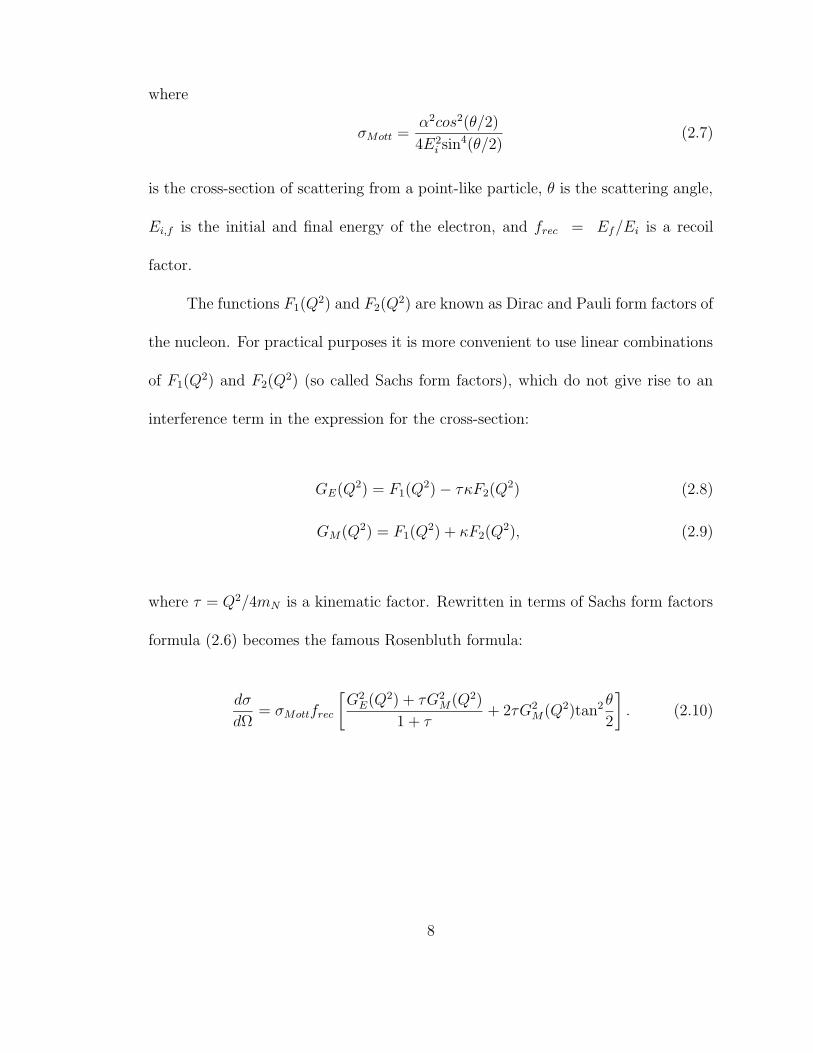
where
σMott =α2cos2(θ/2)
4E2i sin4(θ/2)
(2.7)
is the cross-section of scattering from a point-like particle, θ is the scattering angle,
Ei,f is the initial and final energy of the electron, and frec = Ef/Ei is a recoil
factor.
The functions F1(Q2) and F2(Q
2) are known as Dirac and Pauli form factors of
the nucleon. For practical purposes it is more convenient to use linear combinations
of F1(Q2) and F2(Q
2) (so called Sachs form factors), which do not give rise to an
interference term in the expression for the cross-section:
GE(Q2) = F1(Q
2)− τκF2(Q2) (2.8)
GM(Q2) = F1(Q2) + κF2(Q
2), (2.9)
where τ = Q2/4mN is a kinematic factor. Rewritten in terms of Sachs form factors
formula (2.6) becomes the famous Rosenbluth formula:
dσ
dΩ= σMottfrec
[
G2E(Q2) + τG2M(Q2)
1 + τ+ 2τG2M(Q2)tan2
θ
2
]
. (2.10)
8
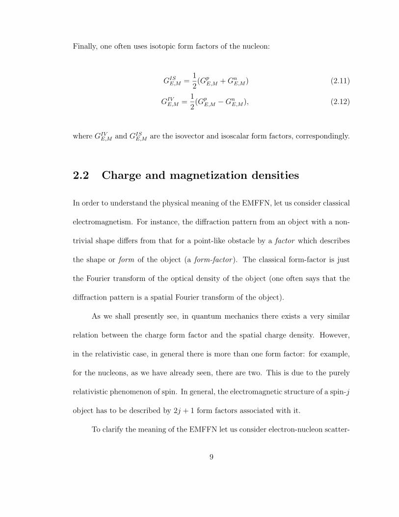
Finally, one often uses isotopic form factors of the nucleon:
GISE,M =
1
2(Gp
E,M +GnE,M) (2.11)
GIVE,M =
1
2(Gp
E,M −GnE,M), (2.12)
where GIVE,M and GIS
E,M are the isovector and isoscalar form factors, correspondingly.
2.2 Charge and magnetization densities
In order to understand the physical meaning of the EMFFN, let us consider classical
electromagnetism. For instance, the diffraction pattern from an object with a non-
trivial shape differs from that for a point-like obstacle by a factor which describes
the shape or form of the object (a form-factor). The classical form-factor is just
the Fourier transform of the optical density of the object (one often says that the
diffraction pattern is a spatial Fourier transform of the object).
As we shall presently see, in quantum mechanics there exists a very similar
relation between the charge form factor and the spatial charge density. However,
in the relativistic case, in general there is more than one form factor: for example,
for the nucleons, as we have already seen, there are two. This is due to the purely
relativistic phenomenon of spin. In general, the electromagnetic structure of a spin-j
object has to be described by 2j + 1 form factors associated with it.
To clarify the meaning of the EMFFN let us consider electron-nucleon scatter-
9
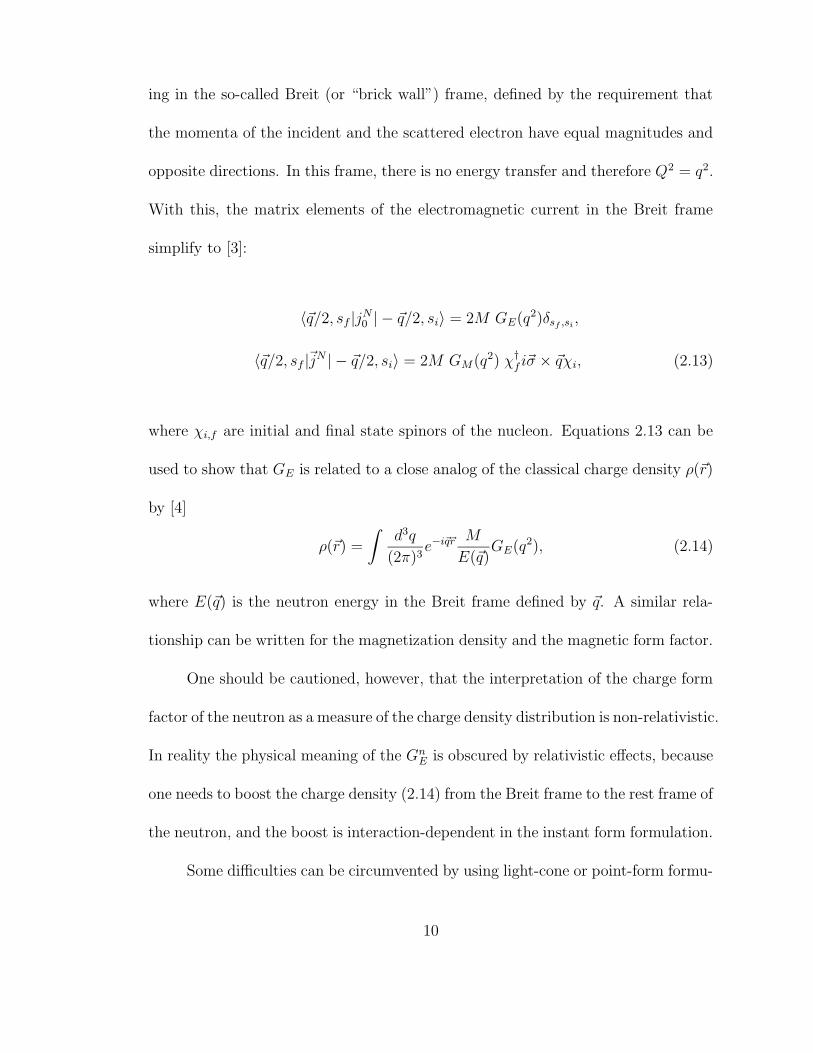
ing in the so-called Breit (or “brick wall”) frame, defined by the requirement that
the momenta of the incident and the scattered electron have equal magnitudes and
opposite directions. In this frame, there is no energy transfer and therefore Q2 = q2.
With this, the matrix elements of the electromagnetic current in the Breit frame
simplify to [3]:
〈~q/2, sf |jN0 | − ~q/2, si〉 = 2M GE(q2)δsf ,si ,
〈~q/2, sf |~jN | − ~q/2, si〉 = 2M GM(q2) χ†f i~σ × ~qχi, (2.13)
where χi,f are initial and final state spinors of the nucleon. Equations 2.13 can be
used to show that GE is related to a close analog of the classical charge density ρ(~r)
by [4]
ρ(~r) =
∫
d3q
(2π)3e−i~q~r M
E(~q)GE(q
2), (2.14)
where E(~q) is the neutron energy in the Breit frame defined by ~q. A similar rela-
tionship can be written for the magnetization density and the magnetic form factor.
One should be cautioned, however, that the interpretation of the charge form
factor of the neutron as a measure of the charge density distribution is non-relativistic.
In reality the physical meaning of the GnE is obscured by relativistic effects, because
one needs to boost the charge density (2.14) from the Breit frame to the rest frame of
the neutron, and the boost is interaction-dependent in the instant form formulation.
Some difficulties can be circumvented by using light-cone or point-form formu-
10

Figure 2.2: Nucleon charge and magnetization densities.
lations, where boost generators are kinematical. However, on the fundamental level,
the problem in the interpretation of form factors is due to the fact that EMFFN
are defined via transition matrix elements between states with different momenta,
and therefore are related to transition (rather than rest frame) charge and mag-
netization densities. Kelly [5] has studied various relativistic prescriptions for the
density extraction recently used in the literature. He found that all of them can be
represented in the form:
ρch(k) = GE(Q2)(1 + τ)λE (2.15)
µρm(k) = GM(Q2)(1 + τ)λM , (2.16)
where the intrinsic form factors ρ(k) are related to the densities by a usual Fourier
11
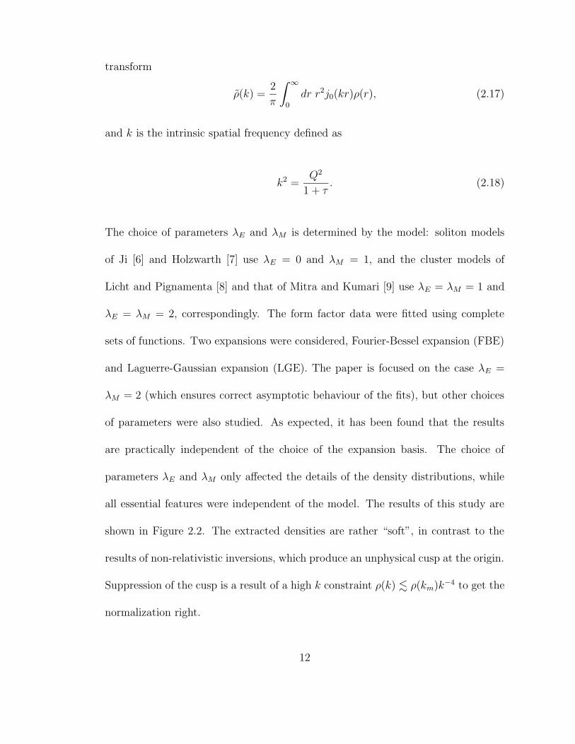
transform
ρ(k) =2
π
∫ ∞
0
dr r2j0(kr)ρ(r), (2.17)
and k is the intrinsic spatial frequency defined as
k2 =Q2
1 + τ. (2.18)
The choice of parameters λE and λM is determined by the model: soliton models
of Ji [6] and Holzwarth [7] use λE = 0 and λM = 1, and the cluster models of
Licht and Pignamenta [8] and that of Mitra and Kumari [9] use λE = λM = 1 and
λE = λM = 2, correspondingly. The form factor data were fitted using complete
sets of functions. Two expansions were considered, Fourier-Bessel expansion (FBE)
and Laguerre-Gaussian expansion (LGE). The paper is focused on the case λE =
λM = 2 (which ensures correct asymptotic behaviour of the fits), but other choices
of parameters were also studied. As expected, it has been found that the results
are practically independent of the choice of the expansion basis. The choice of
parameters λE and λM only affected the details of the density distributions, while
all essential features were independent of the model. The results of this study are
shown in Figure 2.2. The extracted densities are rather “soft”, in contrast to the
results of non-relativistic inversions, which produce an unphysical cusp at the origin.
Suppression of the cusp is a result of a high k constraint ρ(k) . ρ(km)k−4 to get the
normalization right.
12

2.3 Charge radius of the neutron
If one starts with the Fourier integral representation of the neutron charge form
factor
GE(Q2) =
∫
d3rρ(r)e−i~q~r,
and then expands both sides into a Taylor series around q → 0 (since we are working
in the Breit frame, Q2 = q2 → 0):
GE(Q2) = GE(0) + Q2
dGE(Q2)
dQ2
∣
∣
∣
∣
Q2=0
+ ... = Q2dGE(Q
2)
dQ2
∣
∣
∣
∣
Q2=0
+ ...
e−i~q·~r = 1− i~q · ~r + 1
2(i~q · ~r)2 + ...
and calculates resulting integrals, it is straightforward to see that the first two terms
on the right hand side vanish (first one due to zero net charge and the second one
due to parity considerations), whereas for the remaining terms one has:
Q2dGE
dQ2
∣
∣
∣
∣
Q2=0
=
∫
1
2(iqr)2 cos2 θ ρ(r)d3r = −2π
3Q2
∫
r4ρ(r)dr = −1
6Q2r2En,
(2.19)
where r2En is the neutron charge radius r2En =∫
r2ρ(r)d3r. Cancelling a factor of Q2
and rearranging the terms we have for the neutron charge radius
r2En = −6 dGE
dQ2
∣
∣
∣
∣
Q2=0
. (2.20)
13
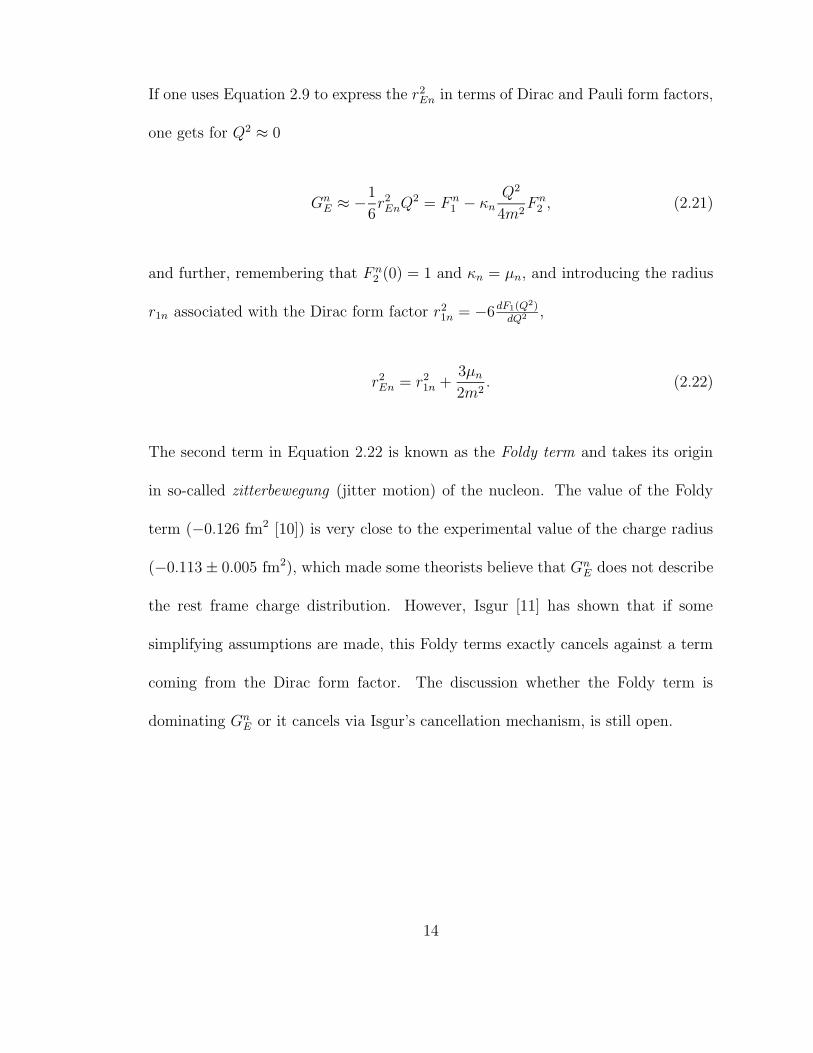
If one uses Equation 2.9 to express the r2En in terms of Dirac and Pauli form factors,
one gets for Q2 ≈ 0
GnE ≈ −
1
6r2EnQ
2 = F n1 − κn
Q2
4m2F n2 , (2.21)
and further, remembering that F n2 (0) = 1 and κn = µn, and introducing the radius
r1n associated with the Dirac form factor r21n = −6dF1(Q2)dQ2
,
r2En = r21n +3µn
2m2. (2.22)
The second term in Equation 2.22 is known as the Foldy term and takes its origin
in so-called zitterbewegung (jitter motion) of the nucleon. The value of the Foldy
term (−0.126 fm2 [10]) is very close to the experimental value of the charge radius
(−0.113± 0.005 fm2), which made some theorists believe that GnE does not describe
the rest frame charge distribution. However, Isgur [11] has shown that if some
simplifying assumptions are made, this Foldy terms exactly cancels against a term
coming from the Dirac form factor. The discussion whether the Foldy term is
dominating GnE or it cancels via Isgur’s cancellation mechanism, is still open.
14

Chapter 3
Previous GnE experiments
3.1 Rosenbluth separation
One simple way of measuring nucleon form factors is suggested by the Rosenbluth
formula (2.10): by measuring the electron-nucleon scattering cross-section for two
different kinematics with common Q2 one obtains two linear equations for squares
of the form factors. This approach has a simple graphical interpretation, with the
help of so-called reduced cross-section
σR =dσ
dΩ
ε(1 + τ)
σMott
= G2M(Q2) + (ε/τ)G2E(Q2),
where ε = [1 + 2(1 + τ) tan2 θe/2]−1 is the transverse polarization of the virtual
photon. If one plots σR versus ε for a fixed Q2 (and therefore τ), then the slope of
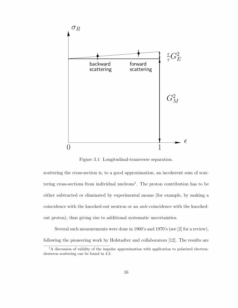
the line is proportional to G2E, while the intercept gives G2M (see Figure 3.1).
This technique can be applied directly to protons by using a hydrogen target.
For the neutron, the simplest target available is deuteron. In the case of quasifree
15
σR
ε
G2M
ετG
2E
scatteringforward
0 1
backwardscattering
Figure 3.1: Longitudinal-transverse separation.
scattering the cross-section is, to a good approximation, an incoherent sum of scat-
tering cross-sections from individual nucleons1. The proton contribution has to be
either subtracted or eliminated by experimental means (for example, by making a
coincidence with the knocked-out neutron or an anti -coincidence with the knocked-
out proton), thus giving rise to additional systematic uncertainties.
Several such measurements were done in 1960’s and 1970’s (see [2] for a review),
following the pioneering work by Hofstadter and collaborators [12]. The results are
1A discussion of validity of the impulse approximation with application to polarized electron-deuteron scattering can be found in 4.2.
16
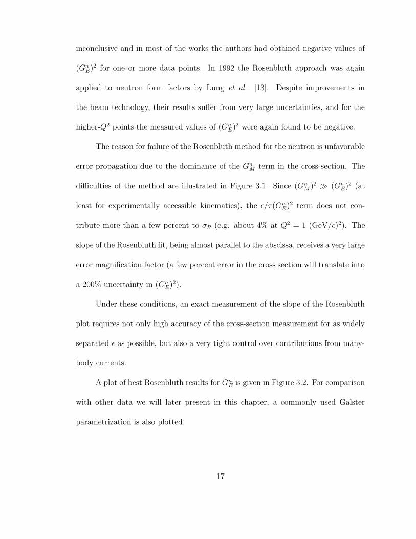
inconclusive and in most of the works the authors had obtained negative values of
(GnE)2 for one or more data points. In 1992 the Rosenbluth approach was again
applied to neutron form factors by Lung et al. [13]. Despite improvements in
the beam technology, their results suffer from very large uncertainties, and for the
higher-Q2 points the measured values of (GnE)2 were again found to be negative.
The reason for failure of the Rosenbluth method for the neutron is unfavorable
error propagation due to the dominance of the GnM term in the cross-section. The
difficulties of the method are illustrated in Figure 3.1. Since (GnM)2 À (Gn
E)2 (at
least for experimentally accessible kinematics), the ε/τ(GnE)2 term does not con-
tribute more than a few percent to σR (e.g. about 4% at Q2 = 1 (GeV/c)2). The
slope of the Rosenbluth fit, being almost parallel to the abscissa, receives a very large
error magnification factor (a few percent error in the cross section will translate into
a 200% uncertainty in (GnE)2).
Under these conditions, an exact measurement of the slope of the Rosenbluth
plot requires not only high accuracy of the cross-section measurement for as widely
separated ε as possible, but also a very tight control over contributions from many-
body currents.
A plot of best Rosenbluth results for GnE is given in Figure 3.2. For comparison
with other data we will later present in this chapter, a commonly used Galster
parametrization is also plotted.
17

0
0.1
0.2
0 0.2 0.4 0.6 0.8 1 1.2 1.4 1.6 1.8 2
Q2 (GeV/c)2
GE
n(Q
2 )
Figure 3.2: Best Rosenbluth data for GnE. Symbols are: filled squares [14], [15]. The
solid line is the standard Galster fit [16].
3.2 Unpolarized elastic e− d scattering
Since the deuteron is a spin-1 particle, the most general form of conserved current
without parity and time-reversal violating terms involves three form factors: GE
(electric), GQ (quadrupole) and GM (magnetic). By introducing structure functions
A(Q2) and B(Q2) one can bring the expression for the e− d scattering cross-section
into a form resembling the Rosenbluth formula:
dσ
dΩ= σMottfrec[A(Q
2) +B(Q2)tan2(θe/2)]. (3.1)
18
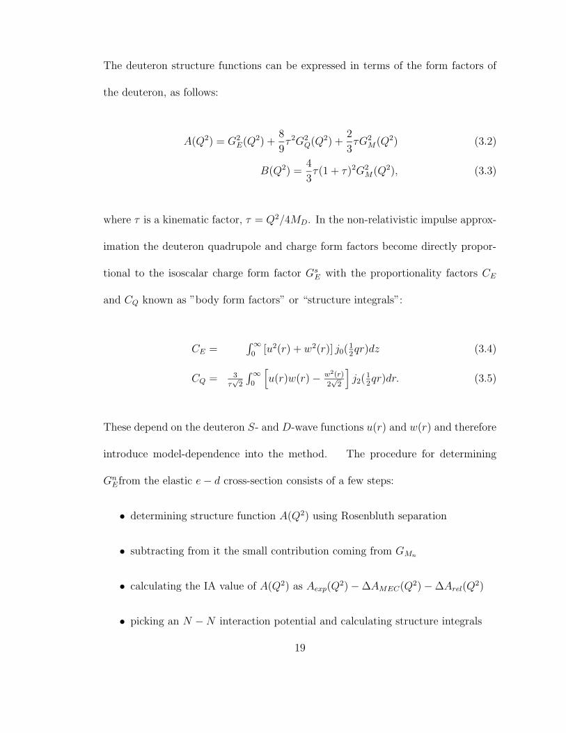
The deuteron structure functions can be expressed in terms of the form factors of
the deuteron, as follows:
A(Q2) = G2E(Q2) +
8
9τ 2G2Q(Q
2) +2
3τG2M(Q2) (3.2)
B(Q2) =4
3τ(1 + τ)2G2M(Q2), (3.3)
where τ is a kinematic factor, τ = Q2/4MD. In the non-relativistic impulse approx-
imation the deuteron quadrupole and charge form factors become directly propor-
tional to the isoscalar charge form factor GsE with the proportionality factors CE
and CQ known as ”body form factors” or “structure integrals”:
CE =∫∞0
[u2(r) + w2(r)] j0(12qr)dz (3.4)
CQ = 3τ√2
∫∞0
[
u(r)w(r)− w2(r)
2√2
]
j2(12qr)dr. (3.5)
These depend on the deuteron S- and D-wave functions u(r) and w(r) and therefore
introduce model-dependence into the method. The procedure for determining
GnEfrom the elastic e− d cross-section consists of a few steps:
• determining structure function A(Q2) using Rosenbluth separation
• subtracting from it the small contribution coming from GMn
• calculating the IA value of A(Q2) as Aexp(Q2)−∆AMEC(Q
2)−∆Arel(Q2)
• picking an N −N interaction potential and calculating structure integrals
19
0
0.05
0.1
0 0.1 0.2 0.3 0.4 0.5 0.6 0.7 0.8 0.9 1
Q2 (GeV/c)2
GE
n(Q
2 )
(a)
0
0.05
0.1
0 0.1 0.2 0.3 0.4 0.5 0.6 0.7 0.8 0.9 1
Q2 (GeV/c)2
GE
n(Q
2 )
(b)
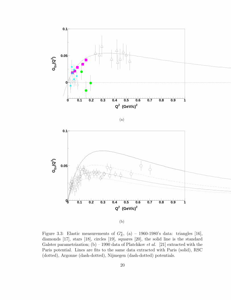
Figure 3.3: Elastic measurements of GnE, (a) – 1960-1980’s data: triangles [16],
diamonds [17], stars [18], circles [19], squares [20], the solid line is the standardGalster parametrization; (b) – 1990 data of Platchkov et al. [21] extracted with theParis potential. Lines are fits to the same data extracted with Paris (solid), RSC(dotted), Argonne (dash-dotted), Nijmegen (dash-dotted) potentials.
20

• calculating the nucleon isoscalar form factor:
G2IS(Q2) = A(Q2)/(C2E(Q
2) + C2Q(Q2))
• choosing a parametrization for GEp and subtracting it from the isoscalar nu-
cleon form factor to get GnE.
First elastic measurements ofGnE were performed in 1960’s atQ2 < 0.2 (GeV/c)2
at SLAC [17] and Orsay [18], [19]. In 1971 the elastic data on GnE has been extended
to higher Q2 by a measurement at DESY by Galster et al. [16]. In a later work
by Simon et al. [20] the data were analyzed with the inclusion of the effects from
meson exchange currents and isobar configurations.
The most recent measurement of GnE using the above approach was carried
out by Platchkov et al. for Q2 up to 0.7 (GeV/c)2 [21]. The relativistic and MEC
effects for the kinematics covered were estimated to be of order of 10%, and were
corrected for, with the systematic uncertainty due to this correction of about 5%.
These uncertainties resulted in an uncertainty of about 20% for the extracted value
of GnE. The results extracted with different N −N interaction potentials are shown
in Figure 3.3(b). The open circles correspond to the Paris potential. For clarity,
for the other potentials only the fits to the extracted data points (not data points
themselves) are shown. As one can see, the model-dependence of the results is of
order of 30− 40%.
21
3.3 Hybrid analysis of the elastic e− d data
The extraction of GnE as described in the previous section relies on the charge and
the quadrupole form factors of the deuteron (after removing a small contribution
from the magnetic form factor to the cross section). Recently it has been shown
that of the two form factors the quadrupole one has less sensitivity to two-body
currents and the choice of the N −N potential [22]. Schiavilla and Sick have used
this fact to extract GnE using the quadrupole form factor GQ and the polarized
observable t20 (we call their approach a hybrid one since it uses both polarized
and unpolarized data). In their analysis, they first fit the world data on the e − d
elastic cross-section with flexible parameterizations for the deuteron form factors,
and then extract GnE by comparing the theoretical predictions of the quadrupole
form factor with the experimental values. The theoretical prediction is the average
of five different theoretical calculations performed with different N −N interaction
potentials. For the proton form factors, the Hoehler parametrization [23] is used,
and GnE is taken in the Galster [16] form 2. A deviation of the theoretical prediction
from the experimental data is taken as an indication of deviation of the GnE from
the adopted parametrization, and the value of GnE is adjusted such that a perfect
agreement between the theoretical and the experimental values of GQ is reached.
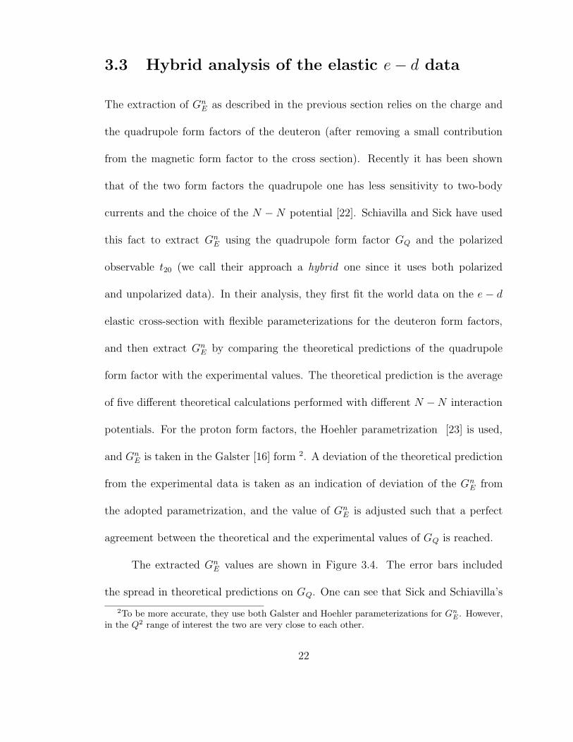
The extracted GnE values are shown in Figure 3.4. The error bars included
the spread in theoretical predictions on GQ. One can see that Sick and Schiavilla’s
2To be more accurate, they use both Galster and Hoehler parameterizations for GnE . However,
in the Q2 range of interest the two are very close to each other.
22

data roughly follow the Galster parameterization, although the error bars are fairly
large (since the points are correlated, they really represent an error band rather
than independent errors).
0
0.05
0.1
0 0.2 0.4 0.6 0.8 1 1.2 1.4 1.6 1.8 2
Q2 (GeV/c)2
GE
n(Q
2 )
Figure 3.4: Sick and Schiavilla’s extraction of Gn. The solid line is the standardGalster parametrization.
3.4 Polarized measurements
To use spin degrees of freedom for determination of GnE was first suggested by
Dombey [24] in late 1960’s. The idea is that various polarization observables (es-
pecially beam-target asymmetry and the recoil polarization) in e− d scattering are
sensitive to GnE. For instance, in plane wave impulse approximation (PWIA) the
23
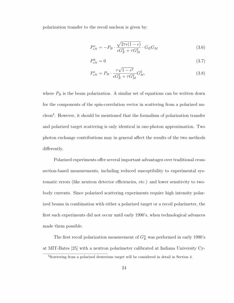
polarization transfer to the recoil nucleon is given by:
P xeN = −PB ·
√
2τε(1− ε)εG2E + τG2M
·GEGM (3.6)
P yeN = 0 (3.7)
P zeN = PB ·
τ√1− ε2
εG2E + τG2MG2M , (3.8)
where PB is the beam polarization. A similar set of equations can be written down
for the components of the spin-correlation vector in scattering from a polarized nu-
cleon3. However, it should be mentioned that the formalism of polarization transfer
and polarized target scattering is only identical in one-photon approximation. Two
photon exchange contributions may in general affect the results of the two methods
differently.
Polarized experiments offer several important advantages over traditional cross-
section-based measurements, including reduced susceptibility to experimental sys-
tematic errors (like neutron detector efficiencies, etc.) and lower sensitivity to two-
body currents. Since polarized scattering experiments require high intensity polar-
ized beams in combination with either a polarized target or a recoil polarimeter, the
first such experiments did not occur until early 1990’s, when technological advances
made them possible.
The first recoil polarization measurement of GnE was performed in early 1990’s
at MIT-Bates [25] with a neutron polarimeter calibrated at Indiana University Cy-
3Scattering from a polarized deuterium target will be considered in detail in Section 4.
24

clotron Facility. Despite low statistical accuracy (due to low 0.8% duty factor of
the accelerator) that experiment was an important demonstration of feasibilty of
the method. Another measurement with this technique was performed at MAMI at
Q2 = 0.15 and Q2 = 0.34 [26]. The most recent polarization transfer GnE experiment
was conducted at the Jefferson Lab at Q2 up to 1.45 [27]. These data provide the
most accurate high-Q2 data on GnE to date.
Early GnE experiments employing the beam-target asymmetry were performed
with the polarized 3He target. In a 3He nucleus, about 86% of the nuclear polar-
ization is carried by a neutron, and therefore it can be used as an effective neutron
target, as originally suggested by Blankleider and Woloshyn [28]. From the exper-
imental point of view, 3He is very convenient (high luminosity and small dilution
afford a very good figure-of-merit). On the other hand, since a 3He nucleus is more
complicated than a deuteron, unfolding nuclear effects becomes a more difficult task.
The analysis of the first measurements with the 3He polarized target neglected
final state interactions and thus resulted in GnE values significantly lower than other
polarized data [29],[30]. A later reanalysis of the data of [30] in [31] with inclusion
of the FSI has brought this data point into a better agreement with the results
obtained with other measurements. Another recent reanalysis of PWIA results from
[32] performed by Bermuth et al. [33] has also somewhat improved the agreement
with the phenomenological Galster parametrization which is roughly followed by
other experimental points at this region.
25

Since the polarized deuteron target is used in the experiment presented in this
dissertation, we shall devote the next chapter to explore this method in detail. Only
two measurements have been taken with this method in the past, one of them being
the 1998 run of the present experiment [34], which yielded an accurate measurement
of GnE at this kinematics (Q2 = 0.5) at that time. In an earlier experiment at
NIKHEF [35] the technique was successfully tested for the first time at Q2 = 0.21.
0
0.05
0.1
0 0.2 0.4 0.6 0.8 1 1.2 1.4 1.6 1.8 2
Q2 [ GeV2 ]
GE
n(Q
2 )
Figure 3.5: Polarized measurements of GnE. Recoil polarimetry data: open circles
[27], open square [25] and open stars [26]. Polarized 3He data: filled square [31],filled circle [33] and filled triangle [29]. Polarized d target: cross-hair [35] andasterisk [34]. The solid line is the standard Galster parametrization.
26
Chapter 4
Experimental technique
4.1 Polarized scattering from a free nucleon
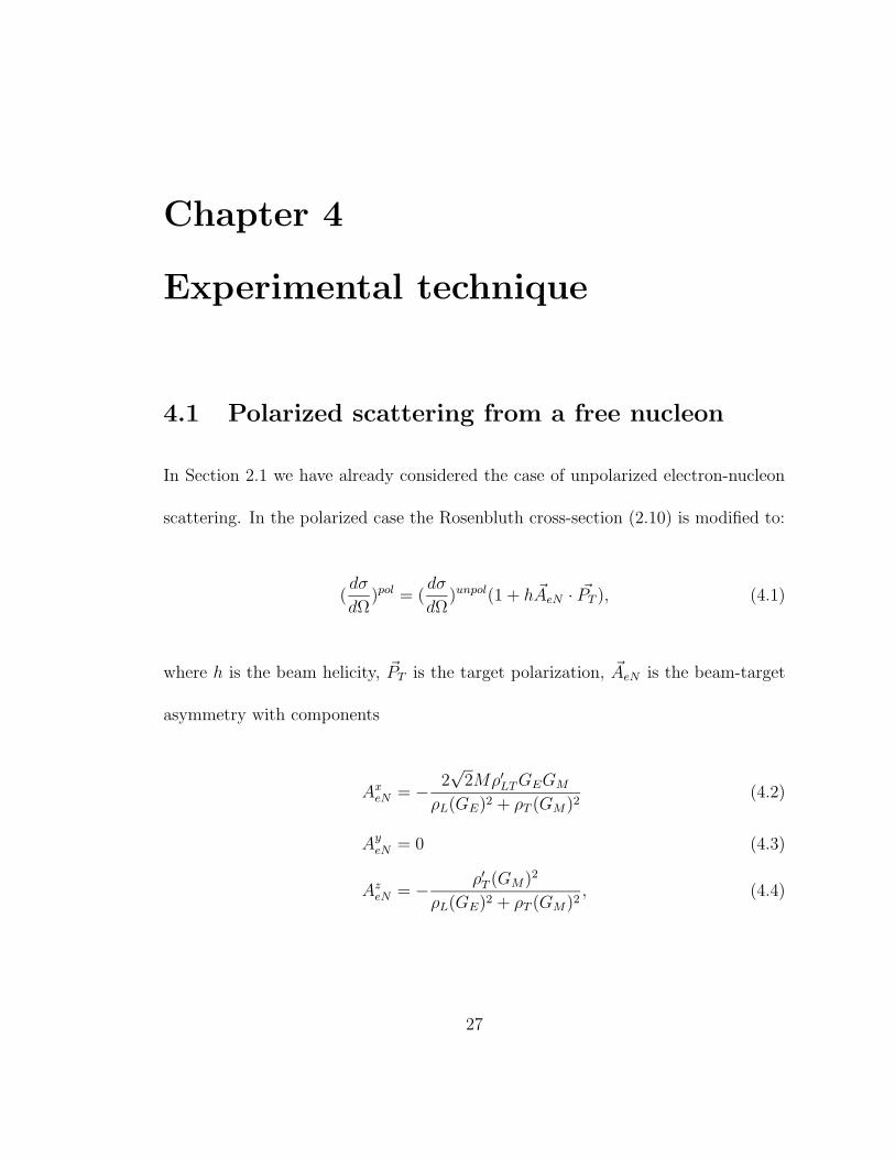
In Section 2.1 we have already considered the case of unpolarized electron-nucleon
scattering. In the polarized case the Rosenbluth cross-section (2.10) is modified to:
(dσ
dΩ)pol = (
dσ
dΩ)unpol(1 + h ~AeN · ~PT ), (4.1)
where h is the beam helicity, ~PT is the target polarization, ~AeN is the beam-target
asymmetry with components
AxeN = − 2
√2Mρ′LTGEGM
ρL(GE)2 + ρT (GM)2(4.2)
AyeN = 0 (4.3)
AzeN = − ρ′T (GM)2
ρL(GE)2 + ρT (GM)2, (4.4)
27

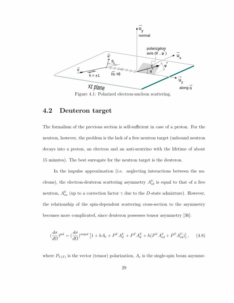
and ρα, ρ′α (α = L, T, LT ) are elements of the virtual photon density matrix
which only depend on the kinematics and the target polarization angles θ∗, φ∗
(see Figure 4.1). As first pointed by Dombey [24], the sensitivity of the asymmetry
(4.2)-(4.4) to the electric form factor can be used for experimental determination of
GnE. This sensitivity is maximizied for the case of in-plane target polarization per-
pendicular to the momentum transfer, i.e. φ∗ = 0 and θ∗ = π/2. The beam-target
asymmetry then simplifies to:
AVen =
−2√
τ(1 + τ) tan(θe/2) GEGM
(GE)2 + τ [1 + 2(1 + τ) tan2(θe/2)](GM)2. (4.5)
On the other hand, from the definition (4.1) the asymmetry can be expressed in
terms of cross-sections for different helicities, σ+ (for h = +1) and σ− (for h = −1):
AVen =
1
PBPT
σ+ − σ−σ+ + σ−
, (4.6)
where we added beam polarization PB to the denominator to account for possibility
of PB < 100%. In the experiment, the cross-sections σ+,− are proportional to
detector yields N+,−, with proportionality factors that carry little or no helicity
dependence, i.e.
AVen =
1
PBPT
N+ −N−N+ +N−
. (4.7)
Equations 4.5 and 4.7 contain all information necessary for experimental determina-
tion of GnE by scattering polarized electron beam off a free polarized nucleon target.
28
θe
e
e'
(q, ω)h = ±1
uy normal
ux
uz
polarization axis (θ∗, φ∗)
φ∗
θ∗
along qxz planeFigure 4.1: Polarized electron-nucleon scattering.
4.2 Deuteron target
The formalism of the previous section is self-sufficient in case of a proton. For the
neutron, however, the problem is the lack of a free neutron target (unbound neutron
decays into a proton, an electron and an anti-neutrino with the lifetime of about
15 minutes). The best surrogate for the neutron target is the deuteron.
In the impulse approximation (i.e. neglecting interactions between the nu-
cleons), the electron-deuteron scattering asymmetry AVed is equal to that of a free
neutron, AVen (up to a correction factor γ due to the D-state admixture). However,
the relationship of the spin-dependent scattering cross-section to the asymmetry
becomes more complicated, since deuteron possesses tensor asymmetry [36]:
(dσ
dΩ)pol = (
dσ
dΩ)unpol
[
1 + hAe + P VAVd + P TAT
d + h(P VAVed + P TAT
ed)]
, (4.8)
where PV (T ) is the vector (tensor) polarization, Ae is the single-spin beam asymme-
29

try, ATd is the single-spin tensor target asymmetry, and AT
ed is the tensor beam-target
asymmetry. Fortunately, in the experiment, the events are normally sampled sym-
metrically in the azimuthal angle, and for this case the contributions from Ae, AVd
and ATed vanish. The remaining AT
d term is suppressed by low tensor polarization of
the deuteron.
Since the deuteron is a weakly bound system, the impulse approximation is a
reasonable first guess. However, for a precise measurement of GnE one needs to take
into account reaction mechanisms listed below.
Meson exchange currents (MEC) are due to the fact that the nucleons in
the deuteron are interacting by meson exchange. Thus, apart from the quasifree
scattering amplitude, there will be contributions from direct coupling to the elec-
tromagnetic current of the exchanged meson. A few basic MEC diagrams are given
on the Fig.4.2.
Isobar currents (IC) arise from intermediate excitation of nucleon resonances
and from the resonance component of the deuteron wavefunction. Unlike the free
case, the scattering from a resonant state cannot be discriminated versus scattering
from the ground-state configuration since the pion, emitted in the resonance decay
may be reabsorbed by the other nucleon.
Final state interactions (FSI) may be important since the final state is a system
of two interacting nucleons rather than two plane waves. To the leading order FSI
30

a) b) c)
Figure 4.2: Meson exchange currents: a) contact diagram, b) pion-in-flight diagram,c) pair diagram.
b)a)
Figure 4.3: Isobar currents: a) coupling to the resonance component of the deuteronwavefunction, b) excitation of the struck nucleon to an intermediate resonance state.
31

can be considered as rescattering of the struck nucleon by the residual nucleus (or
nucleon, in case of the deuteron).
For this experiment relativistic calculations including all these contributions
were performed by H. Arenhovel [37] following formalism developed by him and other
collaborators in [36], [38], [39]. The calculations were carried out over a kinematic
grid representing our experimental acceptance (see Section 6.5.2) for six different
models: PWBA, N + MEC, N + MEC + IC, N + REL, PWBA + REL, N + MEC
+ IC + REL, where PWBA means plane wave Born (or impulse) approximation,
N = PWBA + FSI, and REL means “relativistic effects”.
In Figure 4.4 one can see the sensitivity of the AVed to the charge form fac-
tor of the neutron (a) and interaction effects and relativistic corrections (b). The
asymmetry is plotted versus the angle between the n − p relative momentum and
the momentum transfer ~q in the deuteron center-of-mass frame, θcmnp . The case of
θcmnp = 180 corresponds to the quasifree kinematics, i.e. the struck neutron emitted
along the direction of the momentum transfer. The vertical lines in the Figure 4.4(b)
roughly correspond to the experimental acceptance.
As one can see, at the quasifree kinematics the vector beam-target asymmetry
is both sensitive to GnE and insensitive to many-body currents and relativistic effects,
which makes it ideal for measuring GnE. In order to account for the variation of AV
ed
within the kinematical acceptance, it is necessary to perform acceptance averaging
of the theoretical calculations using Monte Carlo simulations (see Section 6.5).
32

-0.15
-0.1
-0.05
0
0.05
0.1
0 50 100 150 200 250 300 350
θnpcm (deg)
AedV
GEn=1.0×Galster
GEn=0.5×Galster
GEn=1.5×Galster
(a) Sensitivity to the value of the neutron form factor.
-0.15
-0.1
-0.05
0
0.05
0.1
100 120 140 160 180 200 220 240
θnpcm (deg)
AedV
BornNN+MECN+MEC+ICN+MEC+IC+REL
(b) Sensitivity to nuclear and relativistic effects .
Figure 4.4: The vector beam-target asymmetry AVed versus n − p breakup angle in
the deuteron center-of-mass system θcmnp . The case θcmnp = 180 corresponds to the
quasifree kinematics.
33

Chapter 5
Experimental setup
The experimental setup of the 2001 run of E93-026 was very similar to that of
the 1998 run, described in references [40] and [41]. The key elements of the setup
were the same: the High Momentum Spectrometer of Hall C, the UVa polarized
target, the custom built neutron detector and data acquisition (DAQ) electronics.
Important hardware changes since 1998 included:
• redesign of the neutron detector (added new scintillators, changed the layout,
added vertical sticks for position calibration)
• minor upgrades of the target
• removal of the chicane magnet BZ2 that was causing high background in 1998
• DAQ system was reconfigured to take data in an open-trigger mode.
In the remainder of this chapter we will briefly review the main ingredients of the
experimental apparatus.
34
5.1 Polarized electron beam
In this section we will describe the elements responsible for producing, accelerating
and steering the polarized electron beam as well as basic devices used for measuring
its properties.
5.1.1 Accelerator
The Jefferson Lab accelerator was designed to provide a highly polarized continuous
wave electron beam to three experimental halls simultaneously. Polarized electrons
are produced by photo-emission from a strained gallium arsenide cathode. To ensure
simultaneous delivery of the beam to the three physics halls, the photo-cathode is
illuminated by three separate laser systems. The electrons emitted by the three
lasers operating at 499 MHz pulse frequency are combined in a 1497 MHz beam,
from which beams to individual halls are extracted after acceleration.
The initial acceleration to 45 MeV takes places in the injector area. The
orientation of the electron spin in the injector (“injection angle”) determines the
degree of longitudinality of the electron polarization after spin precession in magnetic
elements of arcs and beamlines of the experimental halls. For each configuration of
polarization and energy in the three halls the injection angle needs to be calculated
separately [42].
From the injector the beam is delivered to the north linac, where it is acceler-
35

Figure 5.1: Schematic view of the JLab accelerator (Figure by J. Grames).
ated in radio frequency (RF) cavities by 400 MeV 1. Then the beam goes through
the east recirculation arc to the south linac to be further accelerated by 400 MeV.
Finally, the beam reaches the switchyard, where it can be either extracted to any
of the three experimental halls or steered through the west arc for another pass of
acceleration (up to five passes in total).
The helicity of the beam was pseudo-randomly flipped with the frequency of
30 Hz. The beam current asymmetry (BCA) was minimized with the use of an
asymmetry feedback system. The BCA was typically below 1000 ppm. Other basic
properties of the CEBAF beam delivered to the E93-026 are listed in Table 5.1.
1This is the nominal value. For E93-026 the linac gain was set to 569 MeV.
36
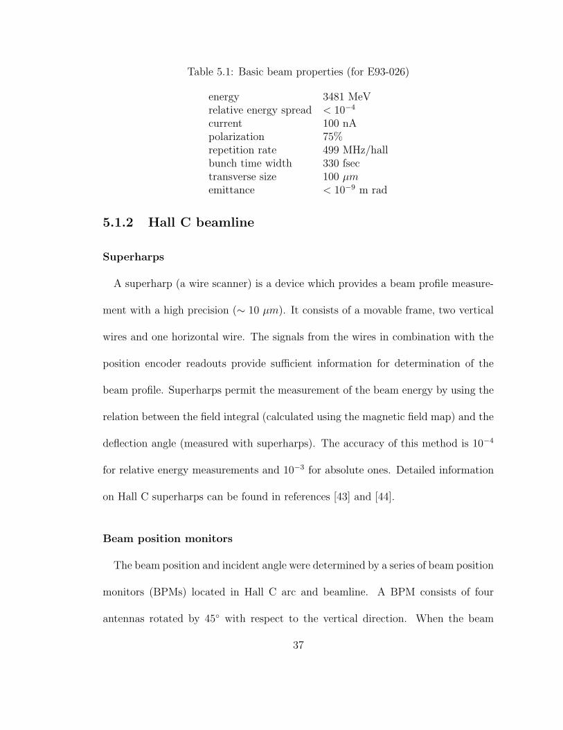
Table 5.1: Basic beam properties (for E93-026)
energy 3481 MeVrelative energy spread < 10−4
current 100 nApolarization 75%repetition rate 499 MHz/hallbunch time width 330 fsectransverse size 100 µmemittance < 10−9 m rad
5.1.2 Hall C beamline
Superharps
A superharp (a wire scanner) is a device which provides a beam profile measure-
ment with a high precision (∼ 10 µm). It consists of a movable frame, two vertical
wires and one horizontal wire. The signals from the wires in combination with the
position encoder readouts provide sufficient information for determination of the
beam profile. Superharps permit the measurement of the beam energy by using the
relation between the field integral (calculated using the magnetic field map) and the
deflection angle (measured with superharps). The accuracy of this method is 10−4
for relative energy measurements and 10−3 for absolute ones. Detailed information
on Hall C superharps can be found in references [43] and [44].
Beam position monitors
The beam position and incident angle were determined by a series of beam position
monitors (BPMs) located in Hall C arc and beamline. A BPM consists of four
antennas rotated by 45 with respect to the vertical direction. When the beam
37

MB
C3C
20H
MB
C3C
20V
IPM
3C20
A
MB
Z3H
05V
IPM
3CH
00
IPM
3CH
00B
IPM
3CH
00A
IHA
3H00
IHA
3H00
A
ITV
3H00
TargetMagnet
BPMs
Beam Correctors
Superharps
Viewer
ToBeamDump
BC
M3
Figure 5.2: Hall C beamline elements [40].
passes through the beamline, each of the antennas picks up the beam’s fundamental
frequency. The digitized signals from the antennas are then used to calculate the
center of gravity in the BPM coordinates, from which the relative beam position in
the beamline is calculated. The absolute position of BPMs was calibrated against
survey measurements. Details on BPM operation can be found in [45].
The beam position near the target was determined by a secondary emission
monitor (SEM) [41]. SEM readings were also used to calibrate the beam position
versus the slow raster current. The SEM and the BPMs provided an accuracy of
about 1 mm.
Beam current monitors
Beam current and total charge passing through the target were measured with
the use of beam current monitors (BCMs). Hall C is equipped with two BCMs.
The BCMs are RF cavities positioned coaxially with the beamline. The RF cavities
serve as cylindrical waveguides whose transverse magnetic mode TM10 is excited by
38
the beam’s fundamental frequency (1497 MHz). The signal is then downconverted
in frequency and sent to an rms-DC converter whose output is proportional to the
beam current.
During data taking, the performance of BCM1 was unstable, and thus all
calculations involving beam charge were based on readings from BCM2. Both BCMs
read 10−15 nA above zero in the absence of the beam. A software cut on the beam
current was used to prevent overestimation of the charge passing through the target
due to these zero readings (see Section 6.2 for details). The calibration of BCMs was
performed using the injector Faraday cup. The accuracy of the BCMs was estimated
to be 5% [46].
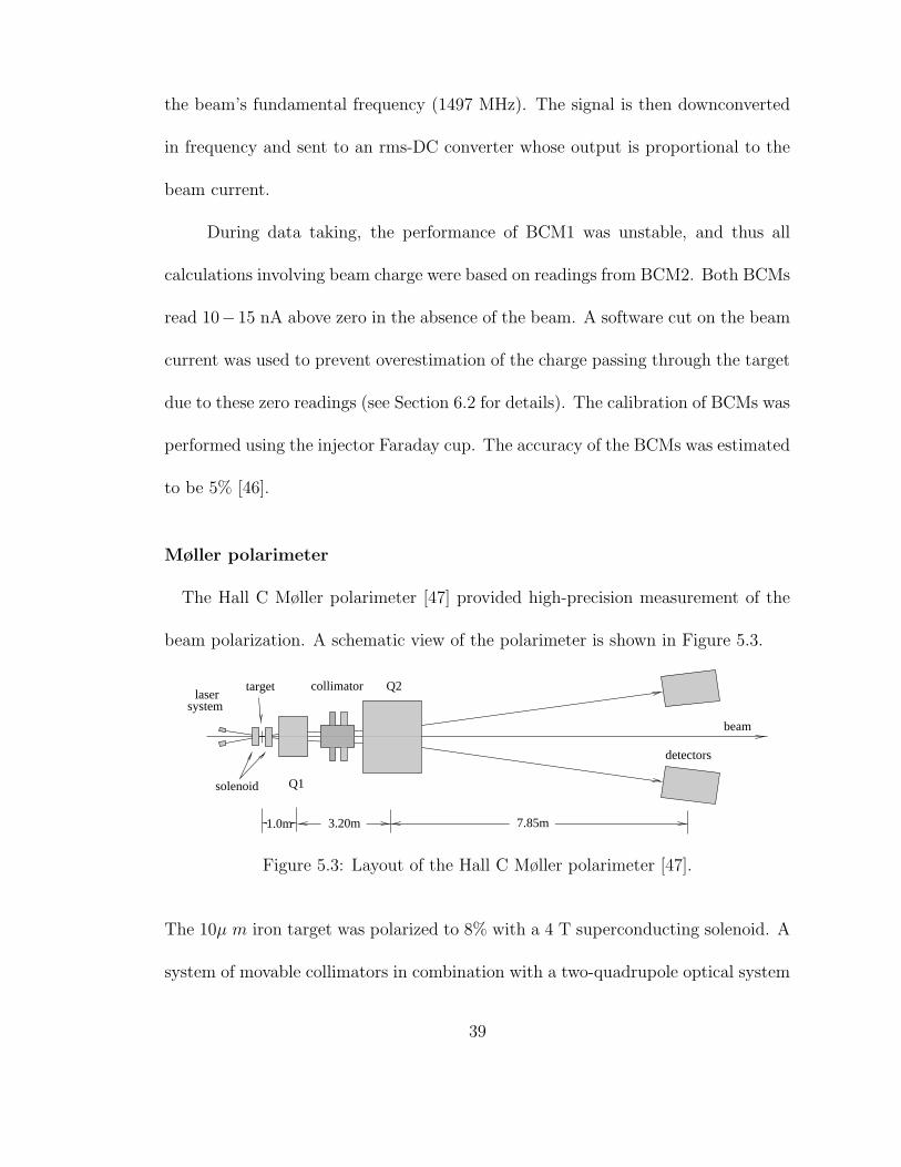
Møller polarimeter
The Hall C Møller polarimeter [47] provided high-precision measurement of the
beam polarization. A schematic view of the polarimeter is shown in Figure 5.3.
systemlaser
1.0m 7.85m
solenoid
collimator
Q1
beam
detectors
Q2
3.20m
target
Figure 5.3: Layout of the Hall C Møller polarimeter [47].
The 10µ m iron target was polarized to 8% with a 4 T superconducting solenoid. A
system of movable collimators in combination with a two-quadrupole optical system
39

was used to suppress Mott background, providing a signal-to-noise ratio of 1000:1.
Recoil and scattered electrons were detected in two lead-glass counters. A statistical
accuracy of about 1% could be obtained in about 20 minutes of measurement time.
5.1.3 Raster magnets
The electron beam was rastered over a 2.2 cm diameter with the Hall C raster
system. The purpose of beam rastering was to ensure uniform distribution of target
polarization over the target face to improve the accuracy of the NMR measurement.
The raster system consists of the slow raster and the fast raster. Each raster sub-
system consists of two magnets driving the beam in x and y directions, a power
resonance loop and a raster pattern generator. The fast raster smeared the beam
over a spot of dimensions of 1 mm×1 mm while the slow raster generated a pseudo-
spiral pattern with the radius of 1.1 cm (see Figure). The amplitude of slow raster
currents was modulated at 0.95 Hz. To minimize induced experimental asymmetries
the frequency of the modulation was synchronized with the beam helicity flip. The
shape of the amplitude modulation was chosen to approximate the A(t) =√
R20 − αt
dependence for which the beam charge deposited at raster radius r approximately
constant (see Figure 5.4). The details of the Hall C raster system can be found in
references [40] and [48].
40
(a) (b)
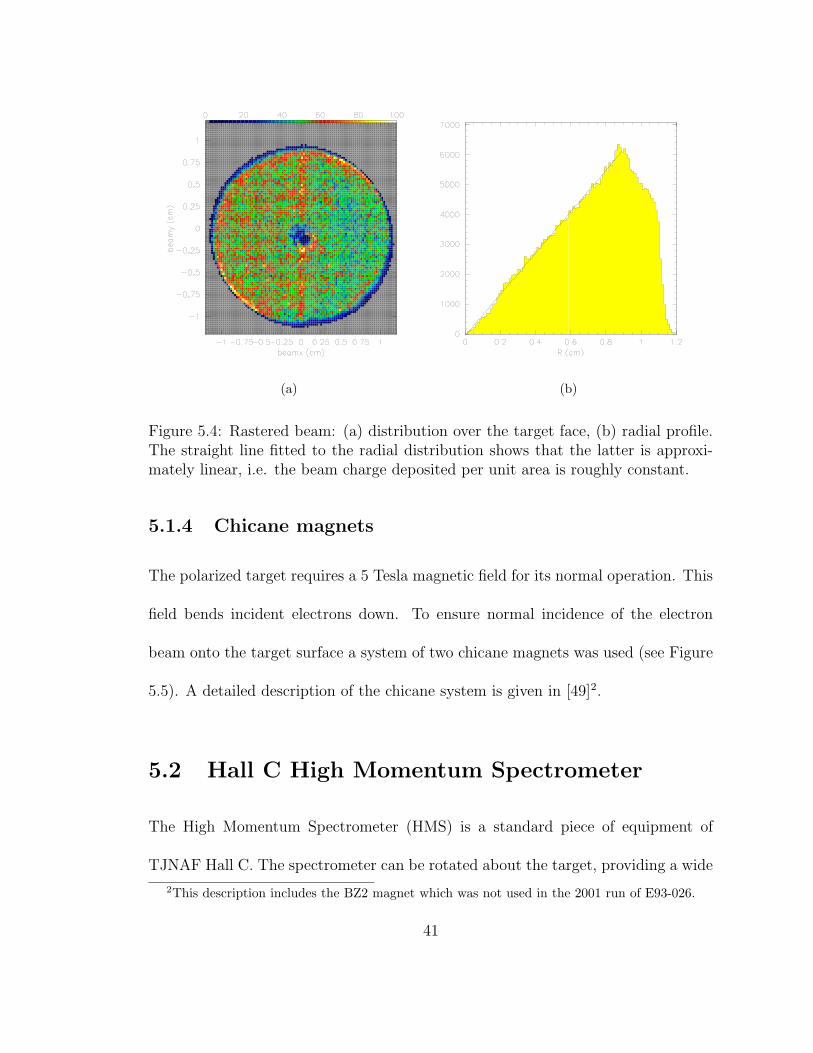
Figure 5.4: Rastered beam: (a) distribution over the target face, (b) radial profile.The straight line fitted to the radial distribution shows that the latter is approxi-mately linear, i.e. the beam charge deposited per unit area is roughly constant.
5.1.4 Chicane magnets
The polarized target requires a 5 Tesla magnetic field for its normal operation. This
field bends incident electrons down. To ensure normal incidence of the electron
beam onto the target surface a system of two chicane magnets was used (see Figure
5.5). A detailed description of the chicane system is given in [49]2.
5.2 Hall C High Momentum Spectrometer
The High Momentum Spectrometer (HMS) is a standard piece of equipment of
TJNAF Hall C. The spectrometer can be rotated about the target, providing a wide
2This description includes the BZ2 magnet which was not used in the 2001 run of E93-026.
41

BESolenoid
BZφ0
φ1
φ2
l1 l2
e−
Figure 5.5: Chicane magnets. The dimensions and angles shown on the picture are:l1 = 4.84 m, l2 = 13.87 m, φ0 = 2.3, φ1 = 0.8, φ2 = 3.1.
range of measurable scattering angles. The basic subsystems of the HMS include
the collimator system, the magneto-optical system and the detector package located
in a shielded hut.
Two different collimators can be installed in the HMS entrance: the octagonal
pion collimator was used for normal data taking, while the sieve slit was used for
spectrometer optics checkout. Three quadrupole magnets and one dipole magnet
comprised the magneto-optical system of the spectrometer. Quadrupole magnets Q1
and Q3 focused rays in the dispersive direction, Q2 focused transverse rays and the
dipole magnet provided a vertical bend of 25 into the detector hut. The detector
package consisted of two drift chambers for tracking, two sets of x-y hodoscopes for
timing and forming the primary trigger, a gas Cerenkov detector and a lead glass
42

27m
Q1 Q2 Q3Dipole
(a)
DC1 DC2S1X S1Y S2X S2Y
CerenkovCalorimeter
(b)
Figure 5.6: Hall C High Momentum Spectrometer: (a) – entire spectrometer, (b) –contents of the detector hut. Note that the calorimeter is tilted in order to preventloss of particles in gaps between the blocks.
shower counter for particle identification. The basic characteristics of the HMS are
listed in Table 5.2.
43

Table 5.2: HMS characteristics.
Maximum central momentum 7.4 GeV/cMomentum resolution 0.04%Solid angle acceptance 5.9 msrScattering angle resolution 0.8 mradOut-of-plane angle resolution 1.0 mradExtended target acceptance 15 cmVertex reconstruction accuracy 5 mm∗∗ Minimum value. In general momentum dependent.
5.3 Polarized target
The UVa cryogenic polarized target has been used in SLAC experiments E143, E155
and E155x prior to being used in E93-026 and is documented in references [40],
[41], [50], [51]. The target was polarized using the dynamic nuclear polarization
(DNP) mechanism (see Appendix A.1). This technique requires the target material
(15ND3) to be placed at a low temperature (about 1K) in a strong magnetic field
(5 Tesla). To transfer the electron polarization to the nuclei, the material must be
additionally radiated by the microwave power. Further, the target polarization must
be continuously monitored. The main components of the target system are shown
in Figure 5.7.
In the remainder of the section we will describe each of these components.
5.3.1 Magnet
The 5 Tesla superconducting magnet was provided by Oxford Instruments. It con-
sisted of two sets of coils, approximately 50 cm in outer diameter and approximately
44

Figure 5.7: Main components of the UVa polarized target.
8 cm apart at the core (Figure 5.8). The shape of magnet was such that its parts
did not interfere with the acceptance of the spectrometer and allowed taking data
in two orientations, perpendicular and parallel to the magnetic field. The magnet
produced a 5 T magnetic field uniform to 1× 10⁻⁴ over the target cell volume and
stable to 1× 10⁻⁶ per hour.
5.3.2 Refrigerator
The 4He evaporation refrigerator was installed vertically along the center of the
magnet. Liquid helium for refrigerator operation was supplied from the magnet
45
MicrowaveInput
NMRSignal Out
Refrigerator
LiquidHelium
Magnet
Target(inside coil)
1 K
NMR Coil
To Pumps
7656A14-94
LN2LN2
To Pumps
B5 T
e–Beam
LiquidHelium
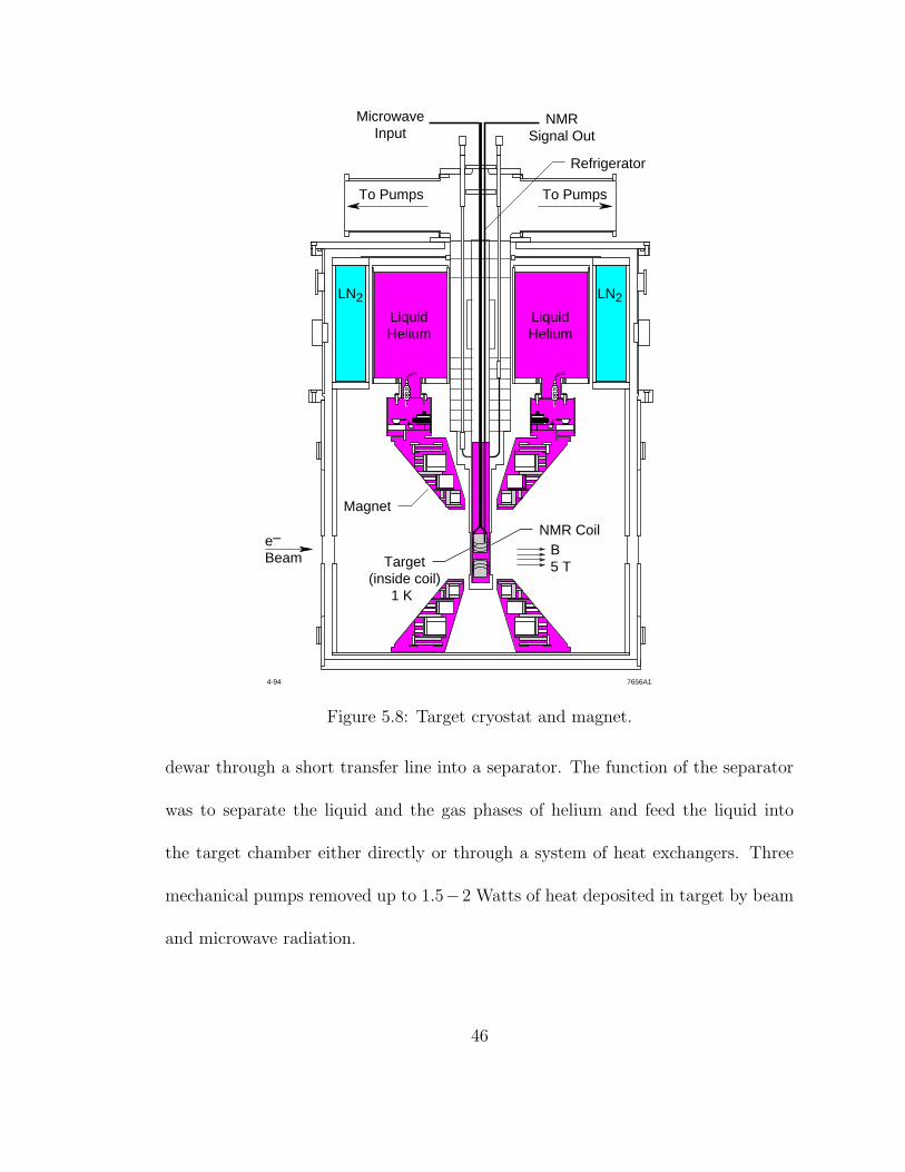
Figure 5.8: Target cryostat and magnet.
dewar through a short transfer line into a separator. The function of the separator
was to separate the liquid and the gas phases of helium and feed the liquid into
the target chamber either directly or through a system of heat exchangers. Three
mechanical pumps removed up to 1.5−2 Watts of heat deposited in target by beam
and microwave radiation.
46
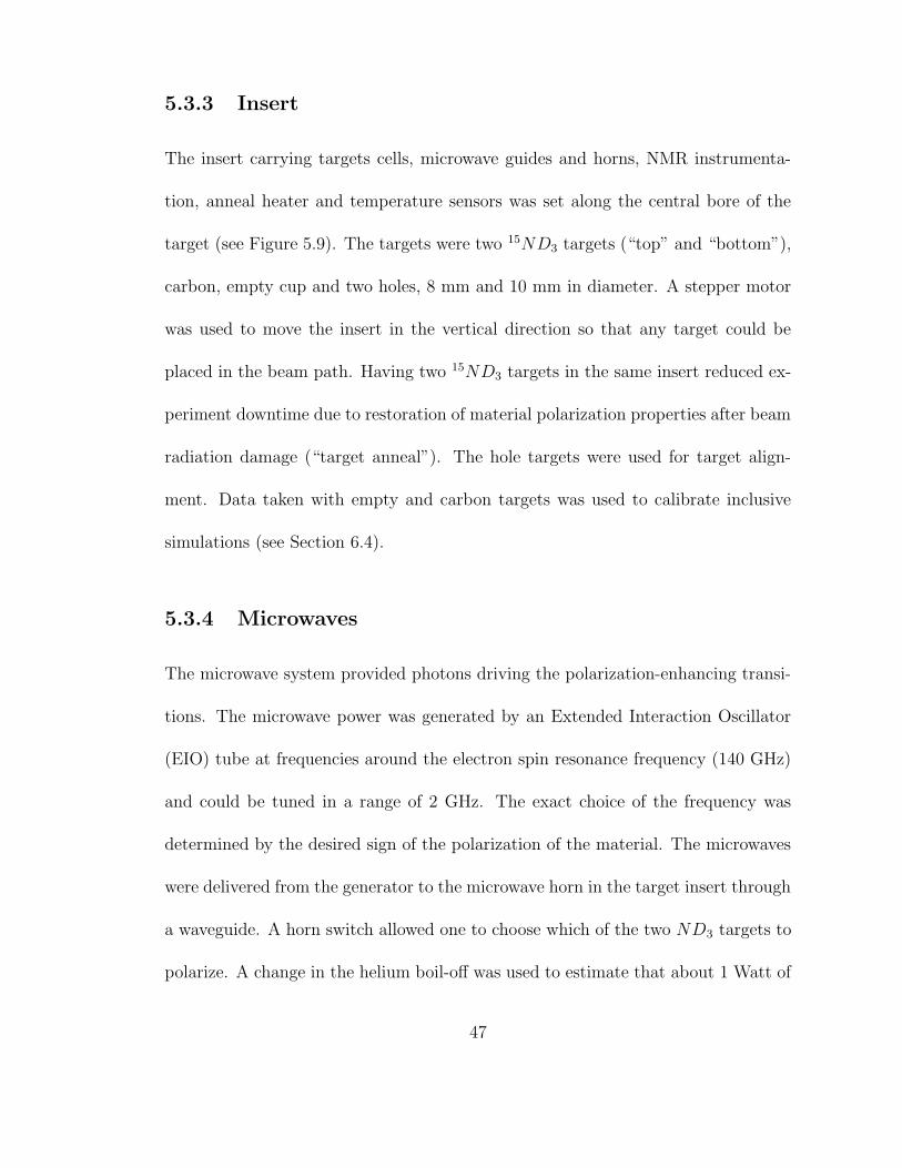
5.3.3 Insert
The insert carrying targets cells, microwave guides and horns, NMR instrumenta-
tion, anneal heater and temperature sensors was set along the central bore of the
target (see Figure 5.9). The targets were two 15ND3 targets (“top” and “bottom”),
carbon, empty cup and two holes, 8 mm and 10 mm in diameter. A stepper motor
was used to move the insert in the vertical direction so that any target could be
placed in the beam path. Having two 15ND3 targets in the same insert reduced ex-
periment downtime due to restoration of material polarization properties after beam
radiation damage (“target anneal”). The hole targets were used for target align-
ment. Data taken with empty and carbon targets was used to calibrate inclusive
simulations (see Section 6.4).
5.3.4 Microwaves
The microwave system provided photons driving the polarization-enhancing transi-
tions. The microwave power was generated by an Extended Interaction Oscillator
(EIO) tube at frequencies around the electron spin resonance frequency (140 GHz)
and could be tuned in a range of 2 GHz. The exact choice of the frequency was
determined by the desired sign of the polarization of the material. The microwaves
were delivered from the generator to the microwave horn in the target insert through
a waveguide. A horn switch allowed one to choose which of the two ND3 targets to
polarize. A change in the helium boil-off was used to estimate that about 1 Watt of
47

Figure 5.9: Target ladder carrying target cells. The targets are (from top to bottom):top 15ND3 (the purple spot is due to the radiation damage), 10 mm hole, 8 mmhole (partially obscured by the microwave horn of the bottom 15ND3 cell), bottom15ND3, carbon and empty.
microwave out of 20 Watts generated reached the target cell.
5.3.5 NMR and data acquisition
The target polarization was continuously measured by the NMR technique (see
Appendix A.2). The NMR system used two copper-nickel coils, one for the bottom
target and one for the top target. The signal from coils was sent through a λ/2 cable
to the Liverpool Q-meter. Calibration constants for the NMR signal were provided
48

by a series of thermal equilibrium (TE) measurements. A target data acquisition
computer used Labview interface to display online values of the target polarization as
well as other critical parameters of the target system (temperature, helium pressure,
microwave frequency and power etc.). The online target polarizations served mostly
for data taking guidance (the figure of merit of the experiment dictates a minimum
polarization below which targets should be switched or annealed) and for a quick
online analysis. The actual target polarization numbers used in calculation of the
AVed were obtained in a full offline analysis (see Section 7.3 for details).
5.3.6 Target material
As the source of polarized deuterons frozen deuterated ammonia was chosen. This
choice was determined by high maximum polarization (up to 40%) and high radia-
tion damage resistance of this material. Additionally, 15ND3, than the usual 14ND3
ammonia, was used, since in 14N both unpaired nucleon spins contribute to the
experimental asymmetries, whereas in 15N only the proton asymmetry is contami-
nated and needs a correction. The purities of the target material were 98% for the
nitrogen and 99% for the deuterium.
The target material was fabricated by shattering frozen ammonia and sifting
the crystals to obtain the fragments of the desired size (1-3 mm). Free paramag-
netic radicals needed by dynamic nuclear polarization were introduced by means
of irradiation in an electron beam. Of the seven batches of material used during
49
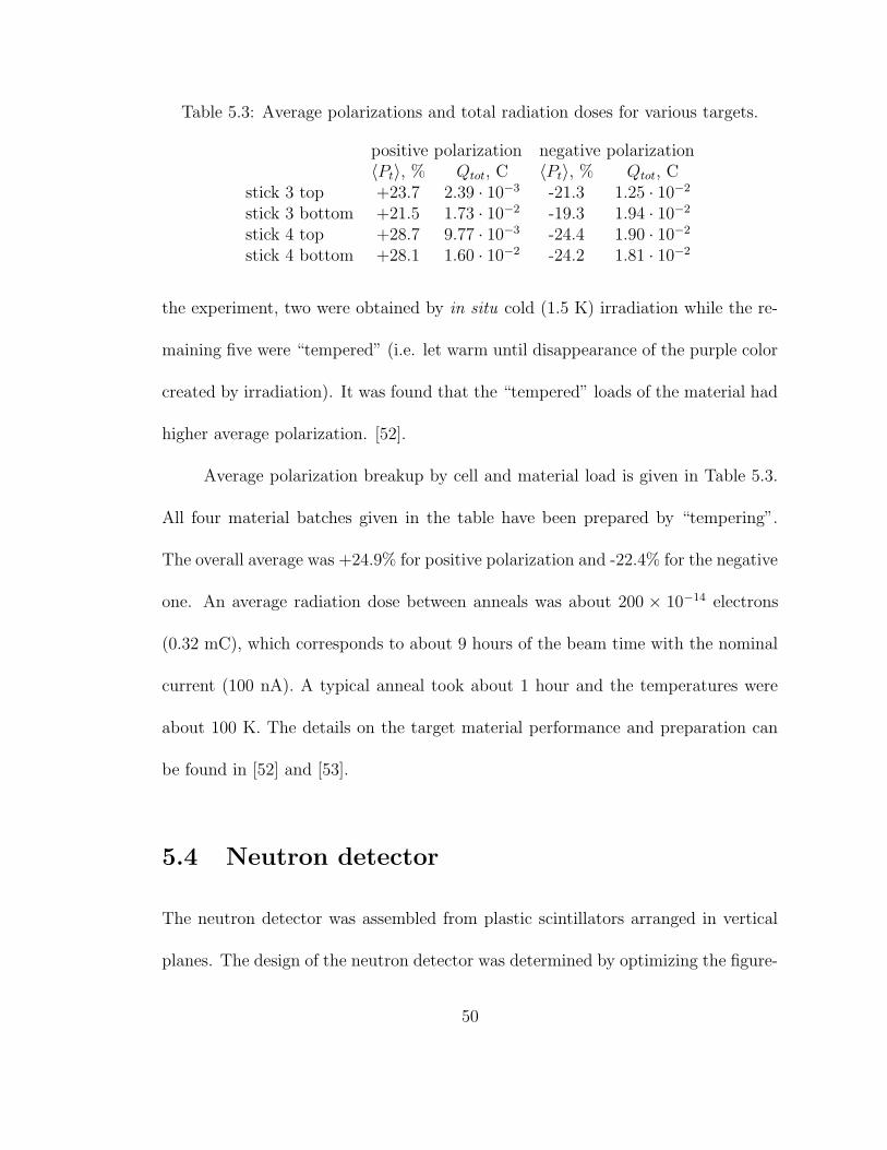
Table 5.3: Average polarizations and total radiation doses for various targets.
positive polarization negative polarization〈Pt〉, % Qtot, C 〈Pt〉, % Qtot, C
stick 3 top +23.7 2.39 · 10−3 -21.3 1.25 · 10−2stick 3 bottom +21.5 1.73 · 10−2 -19.3 1.94 · 10−2stick 4 top +28.7 9.77 · 10−3 -24.4 1.90 · 10−2stick 4 bottom +28.1 1.60 · 10−2 -24.2 1.81 · 10−2
the experiment, two were obtained by in situ cold (1.5 K) irradiation while the re-
maining five were “tempered” (i.e. let warm until disappearance of the purple color
created by irradiation). It was found that the “tempered” loads of the material had
higher average polarization. [52].
Average polarization breakup by cell and material load is given in Table 5.3.
All four material batches given in the table have been prepared by “tempering”.
The overall average was +24.9% for positive polarization and -22.4% for the negative
one. An average radiation dose between anneals was about 200 × 10−14 electrons
(0.32 mC), which corresponds to about 9 hours of the beam time with the nominal
current (100 nA). A typical anneal took about 1 hour and the temperatures were
about 100 K. The details on the target material performance and preparation can
be found in [52] and [53].
5.4 Neutron detector
The neutron detector was assembled from plastic scintillators arranged in vertical
planes. The design of the neutron detector was determined by optimizing the figure-
50

of-merit (FOM) within experimental constraints (number of available scintillators
and slots for neutron detector signals). The simulation for optimizing the neutron
detector FOM used detector efficiencies calculated by KSUVAX program and verti-
cal distributions generated by the customized version of MCEEP (see Section 6.5).
The detector layout as determined from these simulations is shown in Figure 5.10
and described below.
5.4.1 Configuration and position
The front two layers consisted of 1 cm thick scintillators (called paddles) for tagging
charged particles. The bulk of the neutron detector was made up by three kinds
of scintillators called bars (see Table 5.5(a)). The placement of bars was dictated
by considerations of rates. Front planes and top counters tend to have higher rate,
therefore they were filled with narrower bars. To improve the detection and iden-
tification of protons, the first paddle plane and the first bar plane were extended
vertically. In addition to paddles and bars, two plastic scintillators (called sticks)
were included in the detector between the third and fourth bar planes for calibrat-
ing the horizontal position. A detailed description of the neutron detector layout is
given in Table 5.5(b).
Each scintillator had a photomultiplier tube (PMT) attached to each end.
The scintillator and the PMTs were connected through BC-800 lightguides. The
mean of the left and right PMT TDC signals provided the time of the hit while
51
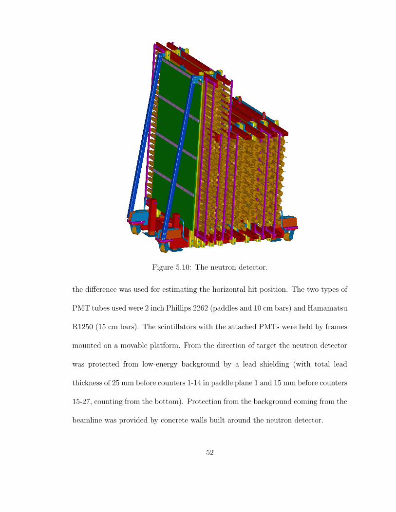
Figure 5.10: The neutron detector.
the difference was used for estimating the horizontal hit position. The two types of
PMT tubes used were 2 inch Phillips 2262 (paddles and 10 cm bars) and Hamamatsu
R1250 (15 cm bars). The scintillators with the attached PMTs were held by frames
mounted on a movable platform. From the direction of target the neutron detector
was protected from low-energy background by a lead shielding (with total lead
thickness of 25 mm before counters 1-14 in paddle plane 1 and 15 mm before counters
15-27, counting from the bottom). Protection from the background coming from the
beamline was provided by concrete walls built around the neutron detector.
52

Table 5.4: Neutron detector scintillators (a) and their layout (b).
type material cross section length phototube qtypaddles BC-408 11 cm× 1 cm 160 cm Phillips 2262 4410 cm bars BC-408 10 cm× 10 cm 160 cm Phillips 2262 4815 cm bars BC-408 trapezoid∗ 160 cm Hamamatsu R1250 2820 cm bars BC-408 trapezoid∗∗ 160 cm Hamamatsu R1250 28sticks BC-408 2 cm× 2 cm 200 cm Phillips 2262 2
∗Top width 12 cm, bottom width 15.4 cm, height 15 cm.∗∗Top width 7.2 cm, bottom width 11.4 cm, height 20 cm.
plane type of counters # of counters packing∗ height1 paddles 27 0.5 cm overlap 61.2 cm2 paddles 17 0.5 cm overlap 61.2 cm3 10 cm bars 26 0.6 cm 66.7 cm4 10 cm bars 16 0.6 cm 67.7 cm5 20 cm bars 18 0.6 cm 65.7 cm6 10 cm & 15 cm bars 10+4 0.6 cm∗∗ 73.8 cm7 15 cm bars 12 0.6 cm 66.6 cm8 15 cm bars 12 0.6 cm 66.6 cm
∗ Vertical distance between adjacent counters.∗∗ 1.6 cm between the 15 cm and 20 cm bars.
The neutron detector was positioned so that the momentum transfer vector
pointed approximately into its center. That allowed to emphasize quasielastic events
and improve the dilution factor. The front plane of the detector was placed at the
distance of 595 cm from the target to allow a comfortable time-of-flight separation
of 8 nanoseconds between gammas from delta electroproduction and nucleons.
53
5.4.2 Gain monitoring
It is possible for the gains of the PMTs to change during the experiment. They may
drift over a long period of time or they may sag due to high rates in the detector.
It is therefore desirable to monitor gains of PMTs. The experiment E93-026 used a
laser pulser for that purpose.
The nitrogen laser was located in a specially designated room in the counting
house. The 337 nm UV light generated by the laser was transformed by the scin-
tillator radiator into visible blue light (λ ∼ 400 nm). This light was transported
by an 80 m long 1 mm diameter silica fiber to the primary distribution box in the
experimental hall, where the signal was split 1:25. Outputs from this box were con-
nected to a 1:64 splitter via a 10 m long 1 mm diameter silica fiber. Outputs from
the splitter were then sent to both ends of the bars. The light output was monitored
by a PIN diode.
By comparing the ADC of the laser signal to its known intensity (300 µJ per
pulse) it is possible to monitor photomultiplier gains and perform energy calibrations
of the neutron detector.
The laser pulser logic for E93-026 is described in the next section. The details
on the design and implementation of the Hall C gain monitoring system can be
found in [54].
54

5.4.3 Gain matching
The gains of bar PMTs were matched using cosmics data. A cosmics trigger was
defined as (OR of top detectors) AND (OR of bottom detectors). Additionally, in
the offline analysis the vertical acceptance was restricted by requiring hits in four
consecutive bars. The gain matching procedure consisted of taking cosmics data at
three different high voltage (HV) settings for each PMT and then fitting the cosmics
peak versus HV. The new HV was chosen such that the cosmics peak was observed
in ADC channel 1100± 100.
The paddles were gain matched using the beam. The bottom part of the
detector was calibrated with the target field turned off because otherwise it does
not have enough statistics. The proton peak was placed in ADC channel 1200±100.
The details of the gain matching procedure can be found in [55].
The thresholds were set to 45 mV for bars and 60 mV for paddles. These
values were obtained by examination of ADC spectra (they were chosen so that the
low energy background did not exceed the height of the proton peak).
5.5 Electronics and data acquisition
In this section we will consider the data acquisition system of the experiment. We
will start by overviewing the electronics for various components of the experimental
setup. Then we will describe how the signals from these components are combined
55
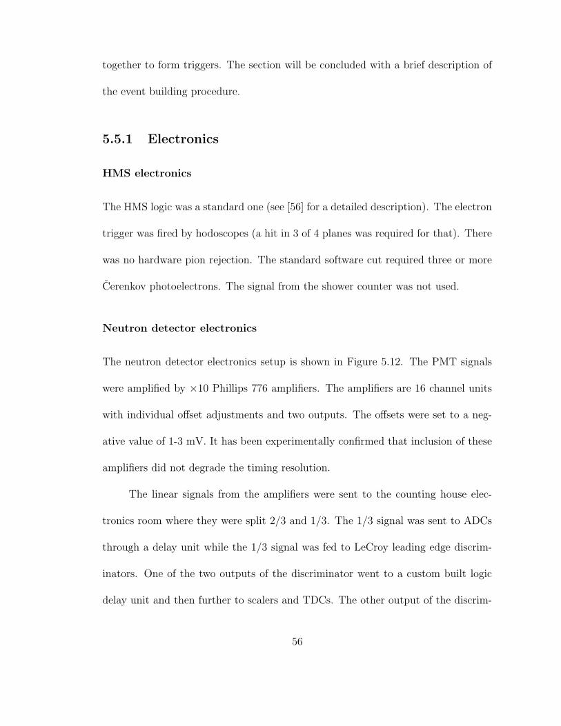
together to form triggers. The section will be concluded with a brief description of
the event building procedure.
5.5.1 Electronics
HMS electronics
The HMS logic was a standard one (see [56] for a detailed description). The electron
trigger was fired by hodoscopes (a hit in 3 of 4 planes was required for that). There
was no hardware pion rejection. The standard software cut required three or more
Cerenkov photoelectrons. The signal from the shower counter was not used.
Neutron detector electronics
The neutron detector electronics setup is shown in Figure 5.12. The PMT signals
were amplified by ×10 Phillips 776 amplifiers. The amplifiers are 16 channel units
with individual offset adjustments and two outputs. The offsets were set to a neg-
ative value of 1-3 mV. It has been experimentally confirmed that inclusion of these
amplifiers did not degrade the timing resolution.
The linear signals from the amplifiers were sent to the counting house elec-
tronics room where they were split 2/3 and 1/3. The 1/3 signal was sent to ADCs
through a delay unit while the 1/3 signal was fed to LeCroy leading edge discrim-
inators. One of the two outputs of the discriminator went to a custom built logic
delay unit and then further to scalers and TDCs. The other output of the discrim-
56

Figure 5.11: HMS trigger electronics. SCIN and STOF are elementary electrontriggers formed by hodoscope signals. ELLO, ELHI and ELREAL are advancedelectron triggers formed from SCIN, STOF, pion rejection and calorimeter signals.In E93-026 only SCIN electron trigger was used.
inator was sent to a LeCroy 4516 logic unit where coincidence between PMT pairs
was formed. The OR output of the LeCroy 4516 module was fired whenever there
was a coincidence in one (or more) out of 16 pairs of PMTs. The signal from the
OR output supplied as input to a JLab custom built coincidence module to form a
coincidence with the HMS PRETRIG (see the next section for data acquisition and
57
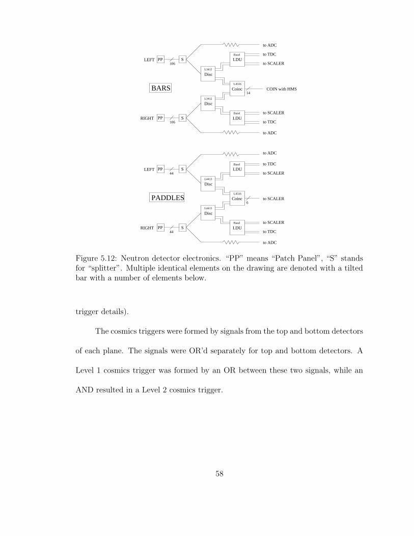
COIN with HMS
S
SPP
PP
S
SPP
PP
Disc
Disc
Coinc
to SCALER
to TDC
to ADC
PADDLES
LDU
LDU
RIGHT
LEFT
Disc
Disc
Coinc
to TDC
to ADC
BARS
LDU
LDU
RIGHT
LEFT
Basel
Basel
44
44
106
106
14
6
to SCALER
to ADC
to TDC
to SCALER
to SCALER
to ADC
to TDC
to SCALER
Basel
Basel
L3412
L3412
L4516
L4413
L4413
L4516
Figure 5.12: Neutron detector electronics. “PP” means “Patch Panel”, “S” standsfor “splitter”. Multiple identical elements on the drawing are denoted with a tiltedbar with a number of elements below.
trigger details).
The cosmics triggers were formed by signals from the top and bottom detectors
of each plane. The signals were OR’d separately for top and bottom detectors. A
Level 1 cosmics trigger was formed by an OR between these two signals, while an
AND resulted in a Level 2 cosmics trigger.
58

Laser electronics
The laser trigger was formed by a coincidence between a photo diode and a photo-
tube (see Figure 5.13).
LINFAN S
M11
N11
ADC
21,1,4(1) DISC TDC
DISC
21,1,11(3) 2/2
PIN diode
DISCLaser PM
S: Splitter21,1,6(4)
LASER(to 8LM)
Figure 5.13: Laser trigger
Scalers
There were three different scaler types used in this experiment: asynchronous scaler,
helicity scaler and event scaler.
Asynchronous scalers were mostly used for counting single rates of the de-
tectors. They were read out every two seconds and were not synchronized to the
helicity flip frequency (thus the name asynchronous). The singles rates from the
scalers were displayed online using the scaler server and a Tcl graphic user interface
(GUI), which allowed one to detect phototube problems in a timely manner.
There were three helicity gated scalers: h+ for positive helicity, h- for negative
helicity and hboth for both helicity states (for consistency check). These scalers
59
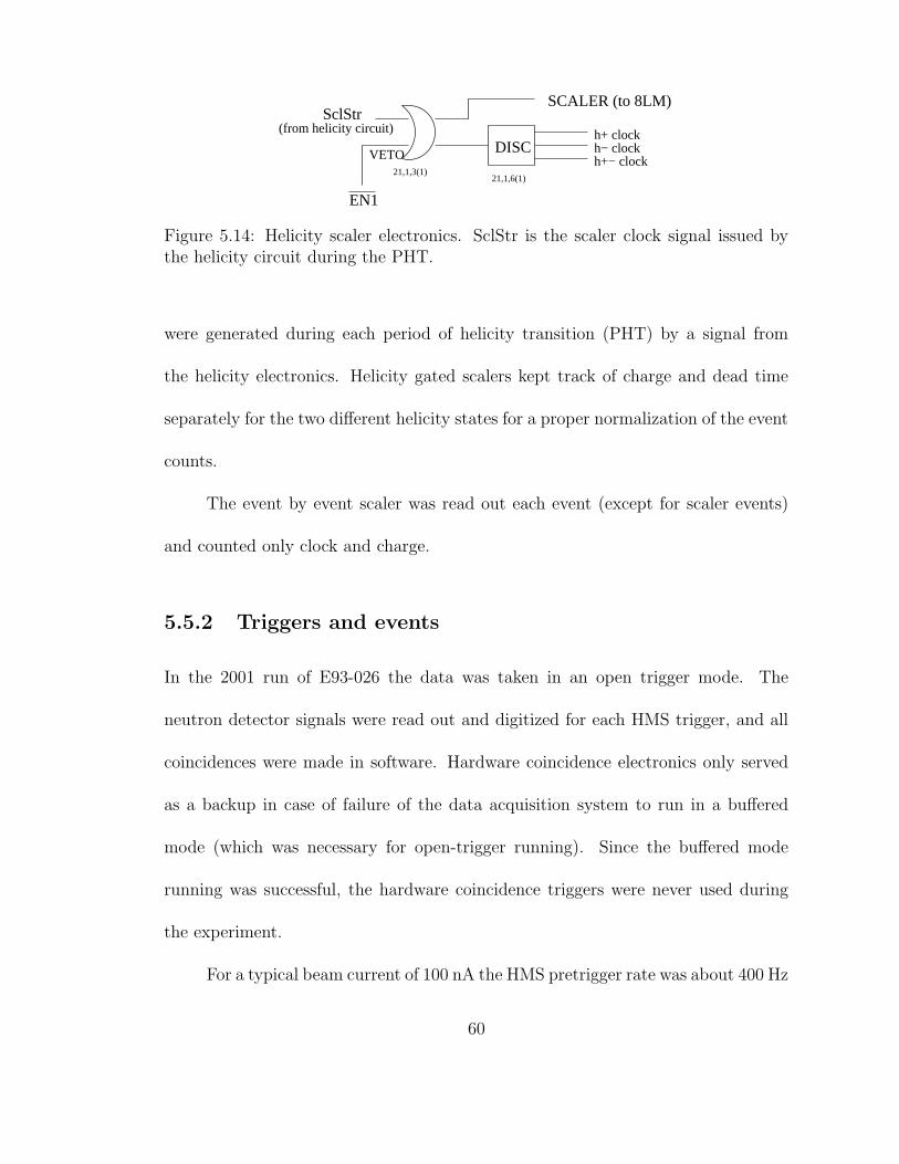
EN1
VETO
SclStrSCALER (to 8LM)
h+ clockh− clockh+− clock
DISC(from helicity circuit)
21,1,3(1)21,1,6(1)
Figure 5.14: Helicity scaler electronics. SclStr is the scaler clock signal issued bythe helicity circuit during the PHT.
were generated during each period of helicity transition (PHT) by a signal from
the helicity electronics. Helicity gated scalers kept track of charge and dead time
separately for the two different helicity states for a proper normalization of the event
counts.
The event by event scaler was read out each event (except for scaler events)
and counted only clock and charge.
5.5.2 Triggers and events
In the 2001 run of E93-026 the data was taken in an open trigger mode. The
neutron detector signals were read out and digitized for each HMS trigger, and all
coincidences were made in software. Hardware coincidence electronics only served
as a backup in case of failure of the data acquisition system to run in a buffered
mode (which was necessary for open-trigger running). Since the buffered mode
running was successful, the hardware coincidence triggers were never used during
the experiment.
For a typical beam current of 100 nA the HMS pretrigger rate was about 400 Hz
60

with a computer dead-time of 4.5 %. The electronics dead-time was negligible (see
Subsection 7.7.3).
Trigger logic
Pretriggers3 and triggers were formed by two Octal Logic Matrix elements (see
Figure 5.15) based on signals from experimental subsystems (HMS and neutron
detector electronics) and DAQ signals generated by the Trigger Supervisor (TS).
The DAQ signals are GO (indicates active DAQ system), EN1 (physics triggers
enabled after taking pedestals) and BUSY (DAQ is processing a trigger and is not
open to any other triggers).
In addition to the two physics triggers used in this experiment (hms and cos-
mics), there was a number of auxiliary triggers generated by DAQ, e.g. pedestal
triggers generated in the beginning of each runs to determine ADC pedestals. 4
A pretrigger was fired by a signal from electronics of the relevant subsystem
if the following conditions were fulfilled:
1. DAQ was active (GO signal high)
2. pedestals have already been taken (EN1 signal high)5
3. helicity transition is not occurring (PHT signal low).
3The difference between pretriggers and triggers is due to the busy status of DAQ only. Apretrigger makes a trigger if the BUSY signal is not present
4Other trigger types, such as laser, sos, coin (coincidence between SOS and HMS) or e*B(coincidence between HMS and the neutron detector) were not used in the experiment and willnot be discussed here.
5For a pedestal pretrigger the case must be exactly the opposite, i.e. EN1 has to be low.
61
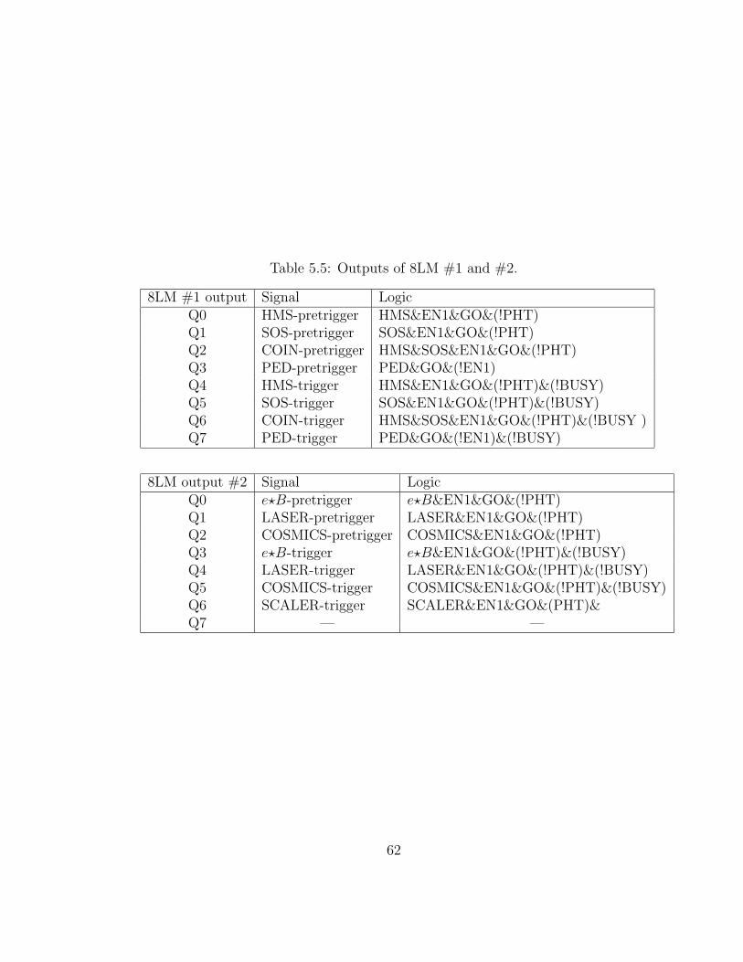
Table 5.5: Outputs of 8LM #1 and #2.
8LM #1 output Signal LogicQ0 HMS-pretrigger HMS&EN1&GO&(!PHT)Q1 SOS-pretrigger SOS&EN1&GO&(!PHT)Q2 COIN-pretrigger HMS&SOS&EN1&GO&(!PHT)Q3 PED-pretrigger PED&GO&(!EN1)Q4 HMS-trigger HMS&EN1&GO&(!PHT)&(!BUSY)Q5 SOS-trigger SOS&EN1&GO&(!PHT)&(!BUSY)Q6 COIN-trigger HMS&SOS&EN1&GO&(!PHT)&(!BUSY )Q7 PED-trigger PED&GO&(!EN1)&(!BUSY)
8LM output #2 Signal LogicQ0 e?B-pretrigger e?B&EN1&GO&(!PHT)Q1 LASER-pretrigger LASER&EN1&GO&(!PHT)Q2 COSMICS-pretrigger COSMICS&EN1&GO&(!PHT)Q3 e?B-trigger e?B&EN1&GO&(!PHT)&(!BUSY)Q4 LASER-trigger LASER&EN1&GO&(!PHT)&(!BUSY)Q5 COSMICS-trigger COSMICS&EN1&GO&(!PHT)&(!BUSY)Q6 SCALER-trigger SCALER&EN1&GO&(PHT)&Q7 — —
62

8LM #2
8LM #1
e*B−pretrig Q1
Q3
Q2
Q4
Q5
Q6
Q7
TS
6,5I1
I2
I3
I4
I5
I6
I7
I8
external
2/2
HMS
1/4
SOS
PED
TS GO
TS EN1
TS BUSY
e*B
COSMICS
LASER
SCALER
PHT
I0 Q0
Q1
Q3
Q2
Q4
Q5
Q6
Q7
I1
I2
I3
I4
I5
I6
I7
I8
I9
I10
SCALER−trig
COSMICS−trig
LASER−trig
e*B−trig
COSMICS−pretrig
LASER−pretrig
HMS−pretrig
SOS−pretrig
COIN−pretrig
PED−pretrig
HMS−trig
SOS−trig
PED−trig
I0 Q0
Q1
Q3
Q2
Q4
Q5
Q6
Q7
I1
I2
I3
I4
I5
I6
I7
I8
I9
I10
COIN−trig
2/2
HADC gates (HMS Hod)
HTDC gates (HMS Hod)
SADC gates (HMS Sh)
STDC gates (HMS Sh)
CADC
ADC gates (N−det)TDC gates (N−det)2/2
Figure 5.15: Trigger setup.
Forming a trigger required fulfilling the same conditions plus DAQ not being busy
processing the previous signal (BUSY signal low).
The outputs of the 8LM modules were fed to the TS. The TS was used to
determine the trigger configuration (enabled triggers and prescale factors) depending
on the run type (main, cosmics, hms only or scalers). Trigger configurations for this
experiment are shown in Table 5.6.
Table 5.6: TS input and configuration. Enabled triggers are indicated with checks.
TS input Trigger main cosmics hms scalers1 HMS
√ √ √2 SOS3 COIN4 e?B
√5 LASER
√ √6 COSMICS
√7 —8 PED
√ √ √9-12 —
63

EPICS
The important experimental quantities (magnet currents, target polarization etc.)
were monitored by the EPICS (for Experimental Physics and Industrial Control
Systems) system. The DAQ queried the EPICS database for these values, formed
an EPICS event and injected the event into the data stream. This occurred on two
time scales depending on expected stability of queried variables: each 2 seconds for
“fast” EPICS variables and each 30 seconds for “slow” EPICS variables.
Event formation
The DAQ system was controlled by CODA software [57]. When TS accepted a
trigger, it sent a signal to read-out controllers (ROCs) which caused readout of ADCs
and TDCs. The ADC and TDC data were collected by ROCs and stored in a buffer,
from where they later forwarded to the Event Builder (EB). The EB assembled the
event fragments together and synchronized them by checking their numbers. In case
of a mismatch an error flag was inserted into the data stream, which allowed the
analysis software to skip bad synchronization events (see Section 6.2). Finally, the
event was written to a hard drive. A background process copied completed runs to
a tape.
64
Chapter 6
Analysis software
This chapter describes software tools used in data analysis. It starts with an
overview of the software components and their interaction with each other. The next
section contains a description of the data-stream preprocessor (syncfilter). Then we
give an overview of the event analyzer1, focusing mainly on HMS and neutron de-
tector event reconstruction. The chapter is concluded with two sections devoted to
inclusive and coincidence simulation packages.
6.1 Overview
The interaction of the software analysis tools with each other is shown in Figure 6.1.
The CODA data files are analyzed with the event analyzer. In order to remove
synchronization errors from the data, the CODA file is piped through the syncfilter.
Additionally, syncfilter reports provide dead-time corrected charge for both helici-
ties. The event analyzer writes reconstructed events into a PAW-compatible ntuple
1Terms event analyzer (or simply analyzer) and analysis engine (or simply engine) refer to thesame code.
65

offlineoffline
filtered eventstream
CODA file
theoretical experimental
normalization
COINCIDENCESIMULATION
SYNCFILTER
EVENTANALYZER
CUTPROCESSOR
INCLUSIVE SIMULATION
packingfraction
HMSsingles rates
dilution factor
cut optimization
coincidencentuples
AVed GE
n
AVed
PT
PB
Figure 6.1: Data analysis software.
66
file. The experimental asymmetries are calculated by the cut processor, whose func-
tion is to count quasi-elastic neutron events for both helicities from the ntuples,
calculate run-by-run asymmetries and then asymmetry averages (by target mate-
rial, beam and target polarization sign etc.). Calculating asymmetries requires the
knowledge of the dilution factor, which is supplied by the coincidence Monte Carlo.
The packing fraction for the dilution factor calculation is obtained using inclusive
simulations.
6.2 Syncfilter
Historically, a need for a data stream preprocessor came about due to the FastBus
synchronization problem (hence the name syncfilter). Later, a number of other
issues, such as non-zero BCM readings, analysis crashes due to missing end-of-run
events, and computer dead-time correction, have come up, and syncfilter proved to
be the most convenient tool for solving them. Let us review different aspects of
syncfilter usage in more detail.
Synchronization errors During E-93026 the DAQ system used several autonomous
crates for data processing, each of them having an independent internal event
counter. Matching of different counters was checked every time a synchronization
event was generated (about every two seconds). In case of a mismatch an error
event was generated, which indicated that all data during the last synchronization
67
interval would have to be discarded. The error event followed the questionable piece
of data in the data stream. However, the analyzer does not have event memory, and
therefore cannot make use of an error warning issued post-factum. This problem
was solved using a data stream preprocessor, which accumulated input data in a
buffer, and inverted the relative order of the error event and the data to which it
referred. In practice, synchronization errors occurred only in a few runs, and even
there the fraction of bad sync events did not exceed one percent.
Missing end-of-run events In case of a ROC crash during a run, the end-of-
run event is normally not inserted into the raw data file, which in its turn made
replay engine crash without producing any meaningful results. To prevent the loss
of these data (which are in most cases perfectly usable), syncfilter was used to insert
fictitious end-of-run events when encountering an unexpected end of the input data.
Low beam current The beam current was not always stable. Low beam current
often correlated with low beam quality. Additionally, the beam current monitors
exhibit significant non-linearity for IBEAM < 50 nA. Therefore, it has been decided
to discard the low current (IBEAM < 50 nA) data with the use of the syncfilter.
Computer dead-time Once the DAQ receives an event, it becomes unable to
process another one for a short period of time (normally, a few nanoseconds). Since
scalers accumulate beam charge regardless to whether or not the DAQ was ready for
taking data, event rates (and therefore measured asymmetries) require a dead-time
68

correction. In E93-026 we used syncfilter to take care of this issue by ignoring the
beam charge accumulated during the busy status of the DAQ.
A detailed description of the syncfilter can be found in [58].
6.3 Hall C replay engine
The event analyzer for E93-026 was based on standard CSOFT package of Hall C.
This software package includes a number of C libraries for processing CODA files
and Fortran utilities for event reconstruction in Hall C spectrometers, HMS and
SOS. Hall C replay engine has a run-time programming mechanism called CEBAF
Test Package (CTP) [59] to dynamically (i.e. without making changes to the source
code) modify:
• parameters used by engine, such as detector configuration, particle masses etc.
• cuts on both raw and analyzed events
• output histograms (conditioned by cuts)
• format of output scaler files
The source code of the analysis engine can be broken down as follows:
Initialization section resets the counters, registers CTP variables, reads the
configuration file, reads in detector decoding map, parameters database and TBPM
69
thresholds from corresponding files and opens the input data stream from a raw
CODA file either directly or piped through the syncfilter.
Non-physics events processing section extracts information stored in control
events, including spectrometer settings, target number, detector high voltages, run
start time etc., and checks synchronization status for sync events.
Physics events analysis section does most of the actual analysis job. It begins
with calculating beam-related quantities (so called “beam reconstruction”) and then
depending on the event type does or skips HMS, neutron detector and coincidence
reconstructions.
Shut-down section saves epics, scaler, statistics and other output files, closes
ntuples, writes out pedestal values, calculates new TDC offset from laser pulser
events and writes the final summary.
6.3.1 HMS event reconstruction
HMS event reconstruction involved two steps: focal plane reconstruction and target
quantities reconstruction. Focal plane reconstruction determines the coordinates
and slopes of the particle track in the spectrometer focal plane and passes them
to the target reconstruction routine, which calculates target track quantities such
70
as vertex coordinates, track slopes at the target and the relative deviation of the
particle momentum from the central momentum of the spectrometer, δHMS.
Focal plane reconstruction
Focal plane reconstruction decodes detector hits and calculates focal plane track
coordinates and slopes. All procedures involved in this step are standard ones and
did not undergo any customization during E93-026 (an outline of standard HMS
reconstruction as well as further references can be found at [40]). If a valid focal
plane track was found, then the algorithm proceeds to the next step:
Target quantities reconstruction
Since HMS optics is very well known, a standard reconstruction (i.e. no target field,
no beam rastering) can be done by simply applying a non-linear matrix transforma-
tion to the four focal plane quantities (coordinates x, y and slopes x′, y′) [60]. For
our experiment, however, the situation is more complicated because of curvature of
charged particle tracks by the target field and a large vertical beam offset due to
beam rastering. To correctly account for these, a doubly nested iterative approach
was adopted.
Reconstruction with a beam offset but without the target field can be done
through the following steps:
1. Do the standard reconstruction assuming no vertical offset (X = 0) to get a
71

first guess of the target quantities.
2. Apply forward transport transformation to the target quantities assuming
X = 0. Repeat the forward transport transformation with the actual vertical
beam offset X = XBEAM and calculate the change in focal planes quantities
due to the beam offset.
3. Apply the focal plane corrections calculated in the previous step and repeat
the backward reconstruction to get the next iteration values of the target
coordinates.
4. Repeat steps 2-4 until difference between two consecutive iterations in δHMS
is less than a pre-defined value.
With the use of this procedure it is now possible to correct for the effect of
the magnetic field as follows:
1. Apply the reconstruction procedure described above to the measured focal
plane quantities to obtain a first guess estimate of the virtual target coordi-
nates2.
2. Drift the electron to a field-free region, then track it back3 into the magnetic
field to the intersection point with the incident beam. That gives the first
guess of the real target coordinates.
2Virtual target coordinates are defined as a set of target coordinate that would result in thesame focal plane quantities as the measured ones if there were no magnetic field present.
3Tracking through the target field was done by solving the differential equations of motion in amagnetic field using Runge-Kutta method.
72
3. Calculate the correction for the virtual beam offset and apply it.
4. Apply the beam-offset reconstruction procedure to the corrected focal plane
quantities to get a better estimate for the virtual target coordinates
5. Drift the electron to the field-free region, then track it back to the intersection
point with the incident beam to get a better estimate for the real target
coordinates.
6. Repeat steps 3-5 until the reconstructed vertical position in the beam plane is
equal to the actual one within a predetermined error.
Normally, the algorithm converged within 5 iterations. The events where conver-
gence is not achieved (which happened in less than 0.1% of cases) were discarded.
6.3.2 Neutron detector event reconstruction
The neutron detector reconstruction can be structured as follows:
1. Single hit analysis
2. Tracking
3. Particle identification.
All code pertaining to the neutron detector side analysis was combined into one
subroutine named n reconstruction. The subroutine begins with clearing all old
event data by calling n reset event. Then it finds all hits with acceptable TDC
73

values and calculates raw TDC differences. After that, the event type is checked
and in case of a laser pulser event the control is passed to special subroutines
(n analyze pindiode and n analyze laser event). If the event is a physics one,
the algorithm proceeds to procedure n time correct. This procedures applies tim-
ing corrections, including event-to event path length, velocity difference and pulse
height (walk) corrections. Having thus concluded analyzing single hits, the subrou-
tine then calculates quantities needed by coincidence reconstruction (layer averages,
coincidence time, and electron momentum transfer in neutron detector coordinates)
and finally does the tracking (ndet tracking) and particle identification (ndet pid)
as described below.
Tracking
The neutron detector tracking routine ndet tracking combines single hits into
one or several tracks. In order to be assigned to the same track single hits need to
have similar meantimes (within ±10 ns) and match the kinematic acceptance.
The main part of the routine consists of two nested loops: the outer one loops
over all bars in all planes, looking for an unused hit to start a track with. The
inner loop checks unused hits in subsequent layers; if a hit falls within the meantime
window and the line connecting the tested hit with the last one on the track falls
within the kinematic acceptance, the hit is added to the track and labeled as used.
After hits have been sorted into tracks, line regression routines are called to fit the
tracks to straight line. Finally, the routine calculates track slopes and checks for a
74

Figure 6.2: A proton event in the neutron detector
fired paddle on the track with energy deposited above minimum. Paddle hits play
a key role in the particle identification process outlined in the next paragraph.
Individual track PID
The neutron detector tracking subroutine ndet tracking starts by testing minimum
track energy and track coincidence time requirements. If both tests are passed, the
routine determines the individual track PID by looking at paddle hits and at the
75

Table 6.1: Event PID
PID code description frequency(%)No track or bad track(s)
0 no track 7.9-1 single bad track 0.2-2 one proton and one neutron track, neither used 5.4-3 multiple tracks, all bad/non-proton 0.0
Good proton1 one proton track – also used for individual tracks 11.92 only reasonable track is proton 0.023 better of 2 proton tracks – based on θnq probability 1.94 better of 2 proton tracks – other has bad χ2 0.025 better of 2 proton tracks – other has bad time 08 best track of several is proton – θnq probability 0
Paddle track9 paddle track 57.7
Good neutron11 one neutron 12.812 only reasonable track is neutron 0.113 better of 2 neutron tracks – based on θnq probability 1.514 better of 2 neutron tracks – other has bad χ2 0.115 better of 2 neutron tracks – other has bad time 0
initial hit of the track (the one in the plane closest to the target). The scheme
of the PID algorithm is given in in Table 6.2. Most events are identified by ab-
sence (neutron) or presence (proton) of a paddle hit, but there are two important
exceptions:
• tracks started at the 1st bar plane4 at counter 17 or above are always labeled
as protons;
• tracks started at bar planes 3-6 are always labeled as neutrons.
4i.e. 3rd detector plane (first two planes are paddles)
76

Table 6.2: Individual track PID
Track started at PID ifplane counter paddle hit no paddle hit
1 17-27 proton proton1 1-16 proton neutron2 any proton neutron3-7 any neutron neutron
Track selection and PID flags
For two-track events, the better track is found according to the algorithm described
below:
• check track PIDs; if same nucleons, proceed, otherwise, discard both tracks;
• check track χ2 (if exactly one track fails the χ2 check, pick the remaining track;
otherwise, proceed with other checks)
• check track time (in the same fashion as above)
• if still have two contenders, pick the track with greater θpq probability.
Multiple (3 or more) track events with heterogeneous nucleons or multi-neutron
tracks were discarded. For multi-proton events, the track with the best θpq proba-
bility was chosen.
A case when a track consisted of paddle hits only (so-called paddle track) was
labeled with a special PID code. Although a significant part of paddle tracks are
77
protons, their contamination by electronics noise makes paddle events essentially
unusable.
The PID codes are summarized in the table 6.1.
6.3.3 Kinematic calculations
Once the tracking has been done, the engine calculates kinematic quantities. There
are two subroutines responsible for this task, h physics (electron arm kinematics)
and c physics (coincidence kinematics).
These calculations use two coordinate systems: the spectrometer (or transport)
one and the beam one. The x axis in both coordinate systems is pointing vertically
down, z is given by the beam momentum for the beam system and the spectrometer
for the spectrometer system, and ~y = ~z × ~x.
Electron arm
The momentum of the incident electron in the beam coordinate system is simply
given by
~k = (0, 0, Evx), (6.1)
where Evx = E −Eloss is the vertex electron energy which differs from the nominal
beam energy E by pre-scattering energy loss Eloss. In the spectrometer coordinate
78

system the scattered electron momentum is given by
Pvx√
1 + (x′)2 + (y′)2(x′, y′, 1), Pvx =
√
E2vx −me2 (6.2)
where x′ and y′ are the electron track slopes, P is the measured electron momentum,
me is the electron mass, Evx = E−∆Eloss and Pvx are vertex energy and momentum
correspondingly, and ∆Eloss is the post-scattering energy loss. The momentum
components in the beam coordinate system are easily obtained by a rotation to the
spectrometer angle θsp:
~k′ =E ′
√
1 + (x′)2 + (y′)2(x′, y′ cos θsp − sin θsp, y
′ sin θsp + cos θsp). (6.3)
The analysis code uses the components of this vector to calculate the scattering
angle θe and the out-of-plane angle φe:
θe = arccosk′z
|~k′|(6.4)
φe = arctank′yk′x. (6.5)
The four-momentum transfer squared Q2 and the invariant mass W are readily
obtained from the four-momenta kµ and k′µ:
Q2 = −qµqµ (6.6)
79
W =√
(qµ + T µ)(qµ + Tµ), (6.7)
where qµ = kµ− k′µ is the four-momentum transfer and Tµ is the four-momentum of
the struck nucleon in the lab frame, Tµ = (M, 0, 0, 0).
Nucleon arm
The subroutine c physics calculates θnq, the angle between the momentum trans-
fer ~q and the track of the nucleon, and θcmnp , the angle between the relative n-p
momentum with respect to the momentum transfer in the n-p center of mass sys-
tem.
The first step in the calculation is forming the unit vector in the direction of
the momentum transfer, q = ~q/|~q|, and then transforming it to the neutron detector
frame, q → q′
~q′ = (qx, qy cos θnDet − qz sin θnDet, qy sin θnDet + qz cos θnDet). (6.8)
The direction of the nucleon track is characterized by vector ∆~n = (∆ x, ∆ y, 1),
where ∆ x and ∆ y are slopes of the nucleon track determined by the tracking
subroutine. Then θnq is simply the angle between ∆~n and ~q′. For convenient can-
cellations, ~q′ is replaced with a collinear vector ∆ q = ~q′/q′z:
cos θnq =∆~n ·∆~q|∆~n| · |∆~q| =
(∆~n)2 + (∆~q)2 − (∆~n−∆~q)2
2|∆~n| · |∆~q| . (6.9)
80

A Lorentz boost to the center of mass system gives then θcmnp [40]:
θcmnp = π − arctan
[
sin θnq
(
ν +MD
Ecmtot
cos θnq −qEn
EcmtotPn
)−1]
, (6.10)
where ν and q are energy and momentum transfer, MD is the mass of the deuteron,
En and Pn are the energy and the nucleon momentum of the knocked out nucleon as
determined from the time of flight, and Ecmtot =
√
(ν +MD)2 − q2 is the total energy
in the center of mass system.
6.4 Inclusive simulations
Inclusive simulation software was designed for calculating packing fraction of the
polarized target (see Section 7.5). The basic components of the software package
include the quasi-free scattering cross-section model, radiative corrections and ac-
ceptance simulation. The simulation was run separately for each target materials.
Contributions from each target material were added with proper weights to represent
kinematic spectra of actual composite targets.
6.4.1 Cross-section model
Inclusive electron scattering cross-sections were simulated using the QFS code by
J. W. Lightbody and J. S. O’Connel [61]. The model assumed incoherent scattering
through following reaction mechanisms:
81
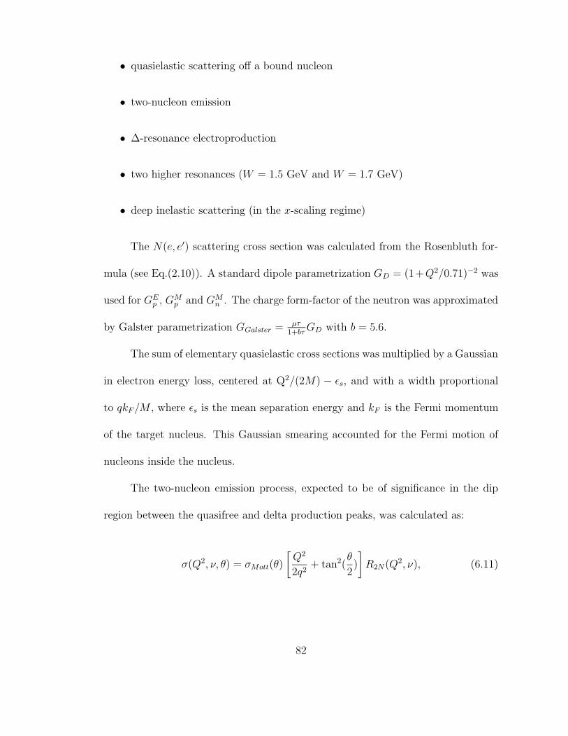
• quasielastic scattering off a bound nucleon
• two-nucleon emission
• ∆-resonance electroproduction
• two higher resonances (W = 1.5 GeV and W = 1.7 GeV)
• deep inelastic scattering (in the x-scaling regime)
The N(e, e′) scattering cross section was calculated from the Rosenbluth for-
mula (see Eq.(2.10)). A standard dipole parametrization GD = (1+Q2/0.71)−2 was
used for GEp , G
Mp and GM
n . The charge form-factor of the neutron was approximated
by Galster parametrization GGalster =µτ1+bτ
GD with b = 5.6.
The sum of elementary quasielastic cross sections was multiplied by a Gaussian
in electron energy loss, centered at Q2/(2M) − εs, and with a width proportional
to qkF/M , where εs is the mean separation energy and kF is the Fermi momentum
of the target nucleus. This Gaussian smearing accounted for the Fermi motion of
nucleons inside the nucleus.
The two-nucleon emission process, expected to be of significance in the dip
region between the quasifree and delta production peaks, was calculated as:
σ(Q2, ν, θ) = σMott(θ)
[
Q2
2q2+ tan2(
θ
2)
]
R2N(Q2, ν), (6.11)
82
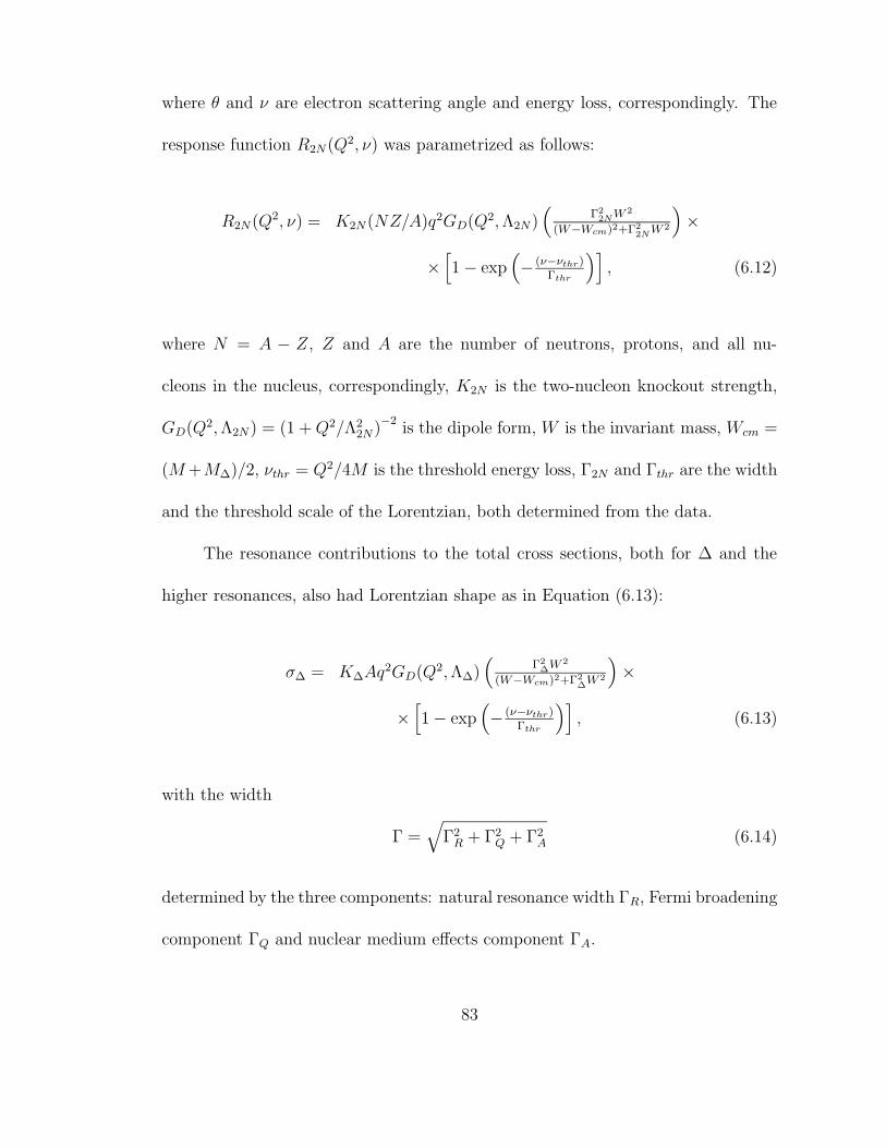
where θ and ν are electron scattering angle and energy loss, correspondingly. The
response function R2N(Q2, ν) was parametrized as follows:
R2N(Q2, ν) = K2N(NZ/A)q
2GD(Q2,Λ2N)
(
Γ22NW 2
(W−Wcm)2+Γ22NW 2
)
×
×[
1− exp(
− (ν−νthr)Γthr
)]
, (6.12)
where N = A − Z, Z and A are the number of neutrons, protons, and all nu-
cleons in the nucleus, correspondingly, K2N is the two-nucleon knockout strength,
GD(Q2,Λ2N ) = (1 +Q2/Λ22N)
−2is the dipole form, W is the invariant mass, Wcm =
(M+M∆)/2, νthr = Q2/4M is the threshold energy loss, Γ2N and Γthr are the width
and the threshold scale of the Lorentzian, both determined from the data.
The resonance contributions to the total cross sections, both for ∆ and the
higher resonances, also had Lorentzian shape as in Equation (6.13):
σ∆ = K∆Aq2GD(Q
2,Λ∆)(
Γ2∆W 2
(W−Wcm)2+Γ2∆W 2
)
×
×[
1− exp(
− (ν−νthr)Γthr
)]
, (6.13)
with the width
Γ =√
Γ2R + Γ2Q + Γ2A (6.14)
determined by the three components: natural resonance width ΓR, Fermi broadening
component ΓQ and nuclear medium effects component ΓA.
83
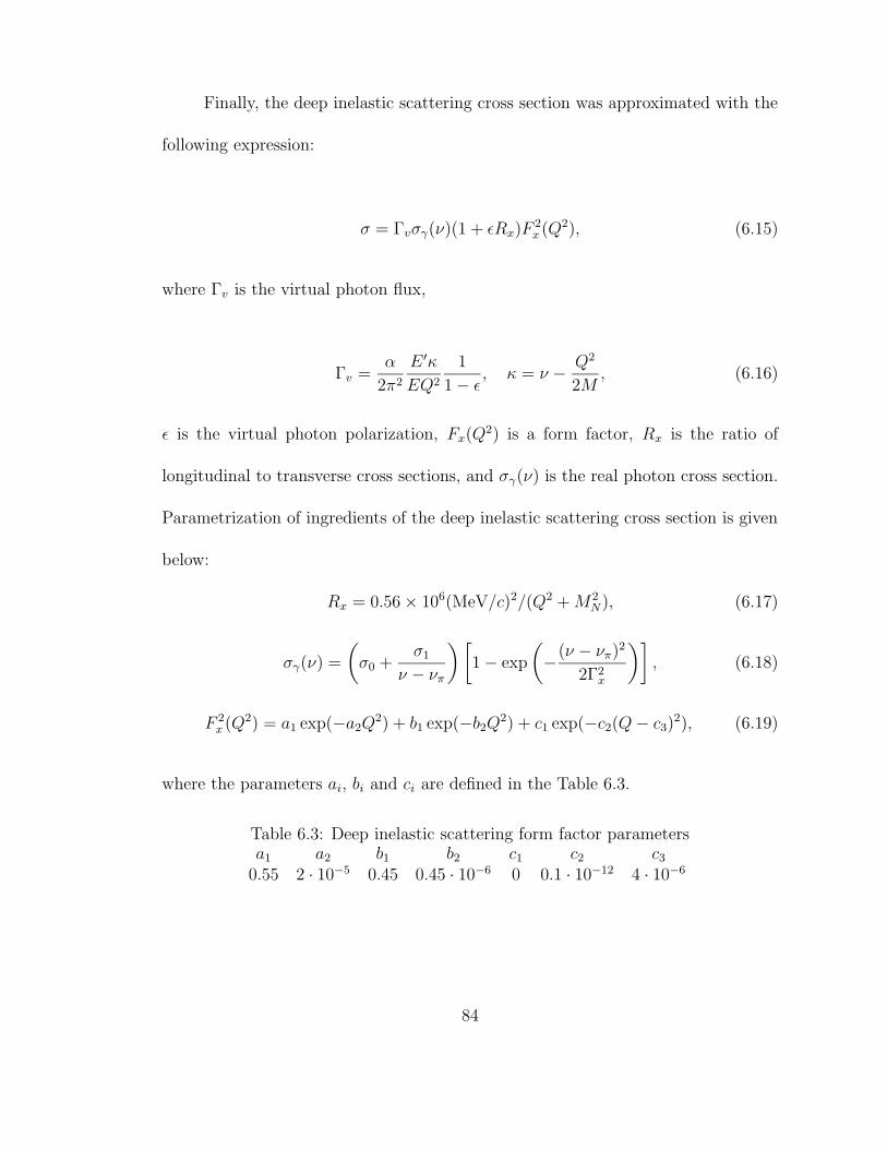
Finally, the deep inelastic scattering cross section was approximated with the
following expression:
σ = Γvσγ(ν)(1 + εRx)F2x (Q
2), (6.15)
where Γv is the virtual photon flux,
Γv =α
2π2E ′κ
EQ21
1− ε , κ = ν − Q2
2M, (6.16)
ε is the virtual photon polarization, Fx(Q2) is a form factor, Rx is the ratio of
longitudinal to transverse cross sections, and σγ(ν) is the real photon cross section.
Parametrization of ingredients of the deep inelastic scattering cross section is given
below:
Rx = 0.56× 10⁶(MeV/c)2/(Q2 +M2N), (6.17)
σγ(ν) =
(
σ0 +σ1
ν − νπ
)[
1− exp
(
−(ν − νπ)22Γ2x
)]
, (6.18)
F 2x (Q2) = a1 exp(−a2Q2) + b1 exp(−b2Q2) + c1 exp(−c2(Q− c3)2), (6.19)
where the parameters ai, bi and ci are defined in the Table 6.3.
Table 6.3: Deep inelastic scattering form factor parametersa1 a2 b1 b2 c1 c2 c30.55 2 · 10−5 0.45 0.45 · 10−6 0 0.1 · 10−12 4 · 10−6
84
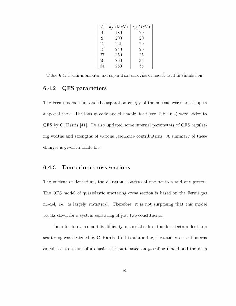
A kf (MeV) εs(MeV )4 180 209 200 2012 221 2015 240 2027 250 2559 260 3564 260 35
Table 6.4: Fermi momenta and separation energies of nuclei used in simulation.
6.4.2 QFS parameters
The Fermi momentum and the separation energy of the nucleus were looked up in
a special table. The lookup code and the table itself (see Table 6.4) were added to
QFS by C. Harris [41]. He also updated some internal parameters of QFS regulat-
ing widths and strengths of various resonance contributions. A summary of these
changes is given in Table 6.5.
6.4.3 Deuterium cross sections
The nucleus of deuterium, the deuteron, consists of one neutron and one proton.
The QFS model of quasielastic scattering cross section is based on the Fermi gas
model, i.e. is largely statistical. Therefore, it is not surprising that this model
breaks down for a system consisting of just two constituents.
In order to overcome this difficulty, a special subroutine for electron-deuteron
scattering was designed by C. Harris. In this subroutine, the total cross-section was
calculated as a sum of a quasielastic part based on y-scaling model and the deep
85
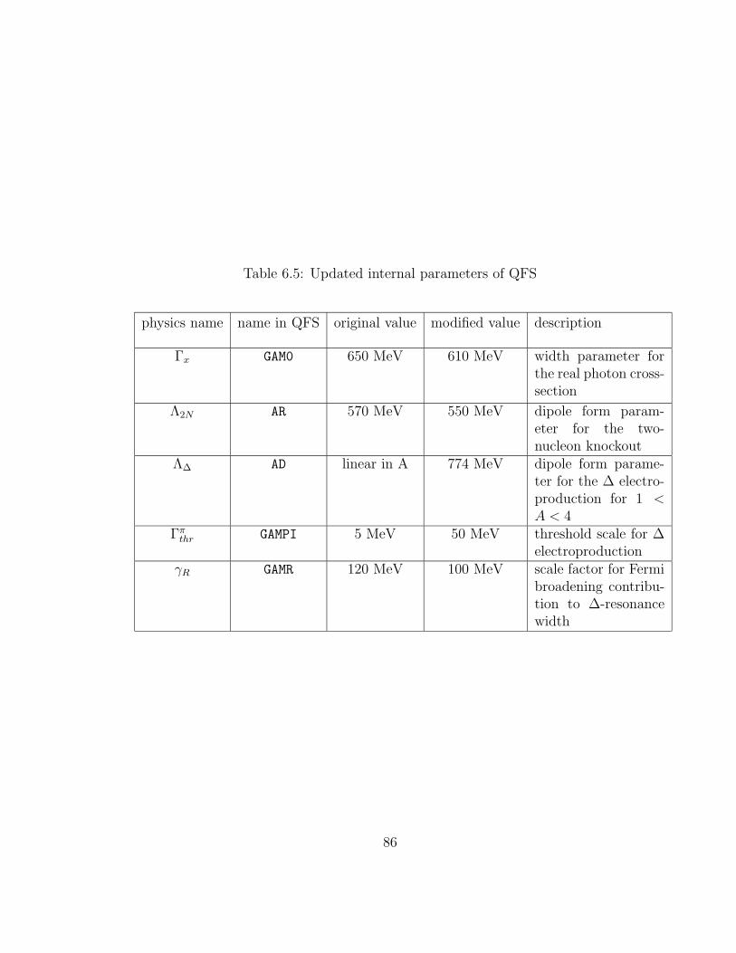
Table 6.5: Updated internal parameters of QFS
physics name name in QFS original value modified value description
Γx GAM0 650 MeV 610 MeV width parameter forthe real photon cross-section
Λ2N AR 570 MeV 550 MeV dipole form param-eter for the two-nucleon knockout
Λ∆ AD linear in A 774 MeV dipole form parame-ter for the ∆ electro-production for 1 <A < 4
Γπthr GAMPI 5 MeV 50 MeV threshold scale for ∆
electroproductionγR GAMR 120 MeV 100 MeV scale factor for Fermi
broadening contribu-tion to ∆-resonancewidth
86

inelastic part. The latter was obtained from a fit to the resonance region data.
The quasielastic contribution to the cross section was calculated using the
Krautschneider momentum distribution [62]:
n(k) = A
[
C +
(
1
k2 + κ1− 1
k2 + κ2
)2]
, (6.20)
where A, κ1 and κ2 are empirical constants and C is the term responsible for rescat-
tering. In our simulation the rescattered term was assumed to be zero.
The results of the simulations for deuterium compared to experimental data
can be found in Fig. 6.3. The agreement is better than 10% except far from the
quasielastic peak, which is adequate for the needs of the experiment.
6.4.4 Radiative effects
The code for calculating both internal and external radiative corrections was pro-
vided by J. Arrington [56]. Unradiated cross-sections were taken as input from QFS.
The calculations were based on a peaking approximation formula derived by Stein
[64] for the particular case of quasi-elastic scattering from a more general formula
by Mo and Tsai [65]:
σ = σsoft + σpre + σpost,
87

Figure 6.3: QFS versus NE4 data for transverse scattering [63].
0
2
4
6
8
10
12
14
0.26 0.28 0.3 0.32 0.34
cros
s-se
ctio
n (n
b/G
eV-s
rad)
E’
NE4QFS
(a) Beam energy E = 841 MeV
0
0.2
0.4
0.6
0.8
1
1.2
1.4
1.6
1.8
0.34 0.36 0.38 0.4 0.42
cros
s-se
ctio
n (n
b/G
eV-s
rad)
E’
NE4QFS
(b) Beam energy E = 1281 MeV
88

σsoft =
(
R∆E
E ′
)b(tb+ta)(∆E
E ′
)b(tb+ta) [
1− ξ/∆E
1− b(ta + tb + 2tr)
]
σ(E,E ′)
σpre =
∫ E−R∆E
Emin(E′)
σ(ε, E ′)
(
E − εE ′R
)b(ta+tr)(E − εE
)b(tb+tr)
[
b(tb + ta)
E − ε φ
(
E − εE
)
+ξ
2(E − ε)2]
dε
σpost =
∫ E′
max
E′+∆E
σ(E, ε′)
(
ε′ − E ′
ε′
)b(ta+tr) [(ε′ − E ′)R
E
]b(tb+tr)
[
b(tb + ta)
ε′ − E ′ φ
(
ε′ − E ′
ε′
)
+ξ
2(ε′ − E ′)2
]
dε′. (6.21)
Here σsoft, σpre and σpost are soft photon, hard photon pre- and post-radiation
contributions to the total radiated cross section correspondingly,
R =MT + 2E sin2 θ
2
MT − 2E ′ sin2 θ2
is a kinematic factor, MT is the target nucleus mass, tb and ta are the target thick-
nesses before and after the interaction point,
tr =α
π
[
log
(
Q2
m2e
)
− 1
]
is the equivalent radiator thickness accounting for internal bremsstrahlung. Other
ingredients of Eq. 6.21 are:
89
b =4
3
[
1 +1
9
Z + 1
Z + ηlog−1(183Z−1/3)
]
,
η = log(1440Z−2/3)/ log(183Z−1/3),
σ(E,E ′) = F (Q2)σ(E,E ′),
F (Q2) = 1 + 0.5772× b(ta + tb) +2α
π(−14
9+
13
12log
Q2
m2)−
− α
2πlog2
E
E ′ +α
π
[
1
6π2 − Φ(cos2 θ/2)
]
,
ξ =πm
2α
ta + tb(Z + η) log(183/Z1/3)
,
and finally, ∆E is the energy cutoff (determined by detector resolution or other
experimental considerations) and
Φ(x) =
∫ x
0
− log |1− y|y
dy
is the Spence function.
The numerical integration was performed using the Romberg technique. The
results were checked by comparing to the cross-section data from the SLAC experi-
ment NE3 (see Fig. 6.4). The agreement is excellent for both radiatively corrected
and uncorrected data.
90
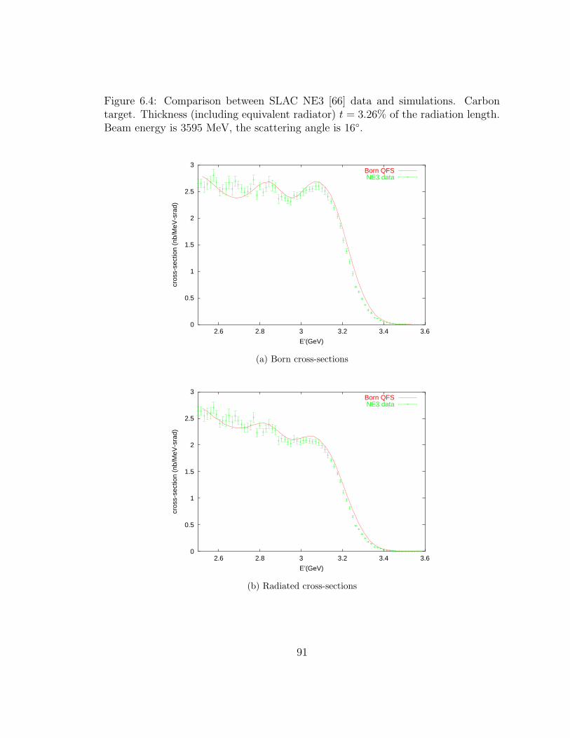
Figure 6.4: Comparison between SLAC NE3 [66] data and simulations. Carbontarget. Thickness (including equivalent radiator) t = 3.26% of the radiation length.Beam energy is 3595 MeV, the scattering angle is 16.
0
0.5
1
1.5
2
2.5
3
2.6 2.8 3 3.2 3.4 3.6
cros
s-se
ctio
n (n
b/M
eV-s
rad)
E’(GeV)
Born QFSNE3 data
(a) Born cross-sections
0
0.5
1
1.5
2
2.5
3
2.6 2.8 3 3.2 3.4 3.6
cros
s-se
ctio
n (n
b/M
eV-s
rad)
E’(GeV)
Born QFSNE3 data
(b) Radiated cross-sections
91
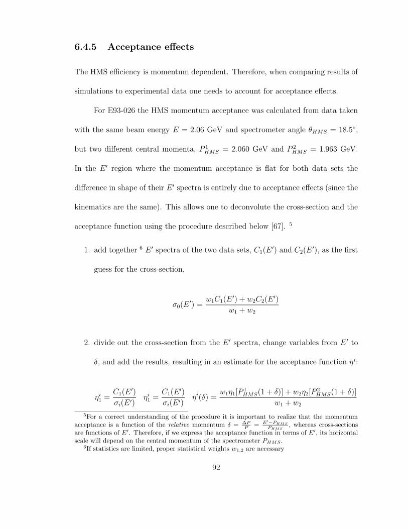
6.4.5 Acceptance effects
The HMS efficiency is momentum dependent. Therefore, when comparing results of
simulations to experimental data one needs to account for acceptance effects.
For E93-026 the HMS momentum acceptance was calculated from data taken
with the same beam energy E = 2.06 GeV and spectrometer angle θHMS = 18.5,
but two different central momenta, P 1HMS = 2.060 GeV and P 2HMS = 1.963 GeV.
In the E ′ region where the momentum acceptance is flat for both data sets the
difference in shape of their E ′ spectra is entirely due to acceptance effects (since the
kinematics are the same). This allows one to deconvolute the cross-section and the
acceptance function using the procedure described below [67]. 5
1. add together 6 E ′ spectra of the two data sets, C1(E′) and C2(E
′), as the first
guess for the cross-section,
σ0(E′) =
w1C1(E′) + w2C2(E
′)
w1 + w2
2. divide out the cross-section from the E ′ spectra, change variables from E ′ to
δ, and add the results, resulting in an estimate for the acceptance function ηi:
ηi1 =C1(E
′)
σi(E ′)ηi1 =
C1(E′)
σi(E ′)ηi(δ) =
w1η1[P1HMS(1 + δ)] + w2η2[P
2HMS(1 + δ)]
w1 + w2
5For a correct understanding of the procedure it is important to realize that the momentumacceptance is a function of the relative momentum δ = ∆P
P= E′
−PHMS
PHMS, whereas cross-sections
are functions of E′. Therefore, if we express the acceptance function in terms of E ′, its horizontalscale will depend on the central momentum of the spectrometer PHMS .
6If statistics are limited, proper statistical weights w1,2 are necessary
92

Figure 6.5: HMS momentum acceptance.
(a) Raw spectra (b) Acceptance-unfolded spectra
Figure 6.6: HMS acceptance effects: E ′ spectra for carbon runs 40466 and 40655(PHMS = 2.06 GeV and PHMS = 1.9627 GeV) before (a) and after (b) unfoldingacceptance effects.
93
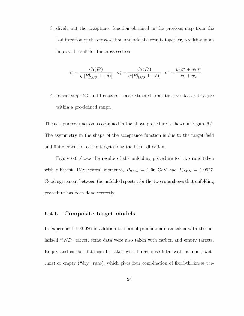
3. divide out the acceptance function obtained in the previous step from the
last iteration of the cross-section and add the results together, resulting in an
improved result for the cross-section:
σi1 =
C1(E′)
ηi[P 1HMS(1 + δ)]σi1 =
C1(E′)
ηi[P 1HMS(1 + δ)]σi =
w1σi1 + w1σ
i1
w1 + w2
4. repeat steps 2-3 until cross-sections extracted from the two data sets agree
within a pre-defined range.
The acceptance function as obtained in the above procedure is shown in Figure 6.5.
The asymmetry in the shape of the acceptance function is due to the target field
and finite extension of the target along the beam direction.
Figure 6.6 shows the results of the unfolding procedure for two runs taken
with different HMS central momenta, PHMS = 2.06 GeV and PHMS = 1.9627.
Good agreement between the unfolded spectra for the two runs shows that unfolding
procedure has been done correctly.
6.4.6 Composite target models
In experiment E93-026 in addition to normal production data taken with the po-
larized 15ND3 target, some data were also taken with carbon and empty targets.
Empty and carbon data can be taken with target nose filled with helium (“wet”
runs) or empty (“dry” runs), which gives four combination of fixed-thickness tar-
94
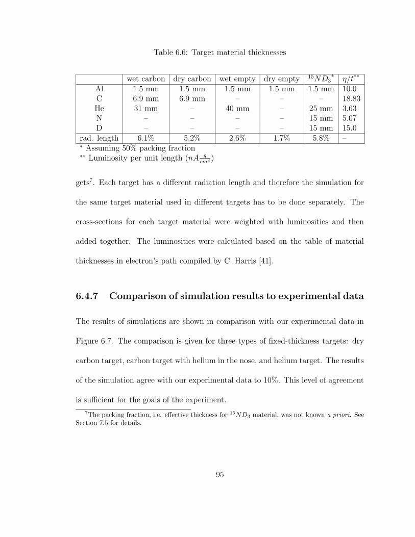
Table 6.6: Target material thicknesses
wet carbon dry carbon wet empty dry empty 15ND3∗
η/t∗∗
Al 1.5 mm 1.5 mm 1.5 mm 1.5 mm 1.5 mm 10.0C 6.9 mm 6.9 mm – – – 18.83He 31 mm – 40 mm – 25 mm 3.63N – – – – 15 mm 5.07D – – – – 15 mm 15.0
rad. length 6.1% 5.2% 2.6% 1.7% 5.8% –∗ Assuming 50% packing fraction∗∗ Luminosity per unit length (nA g
cm3)
gets7. Each target has a different radiation length and therefore the simulation for
the same target material used in different targets has to be done separately. The
cross-sections for each target material were weighted with luminosities and then
added together. The luminosities were calculated based on the table of material
thicknesses in electron’s path compiled by C. Harris [41].
6.4.7 Comparison of simulation results to experimental data
The results of simulations are shown in comparison with our experimental data in
Figure 6.7. The comparison is given for three types of fixed-thickness targets: dry
carbon target, carbon target with helium in the nose, and helium target. The results
of the simulation agree with our experimental data to 10%. This level of agreement
is sufficient for the goals of the experiment.
7The packing fraction, i.e. effective thickness for 15ND3 material, was not known a priori. SeeSection 7.5 for details.
95
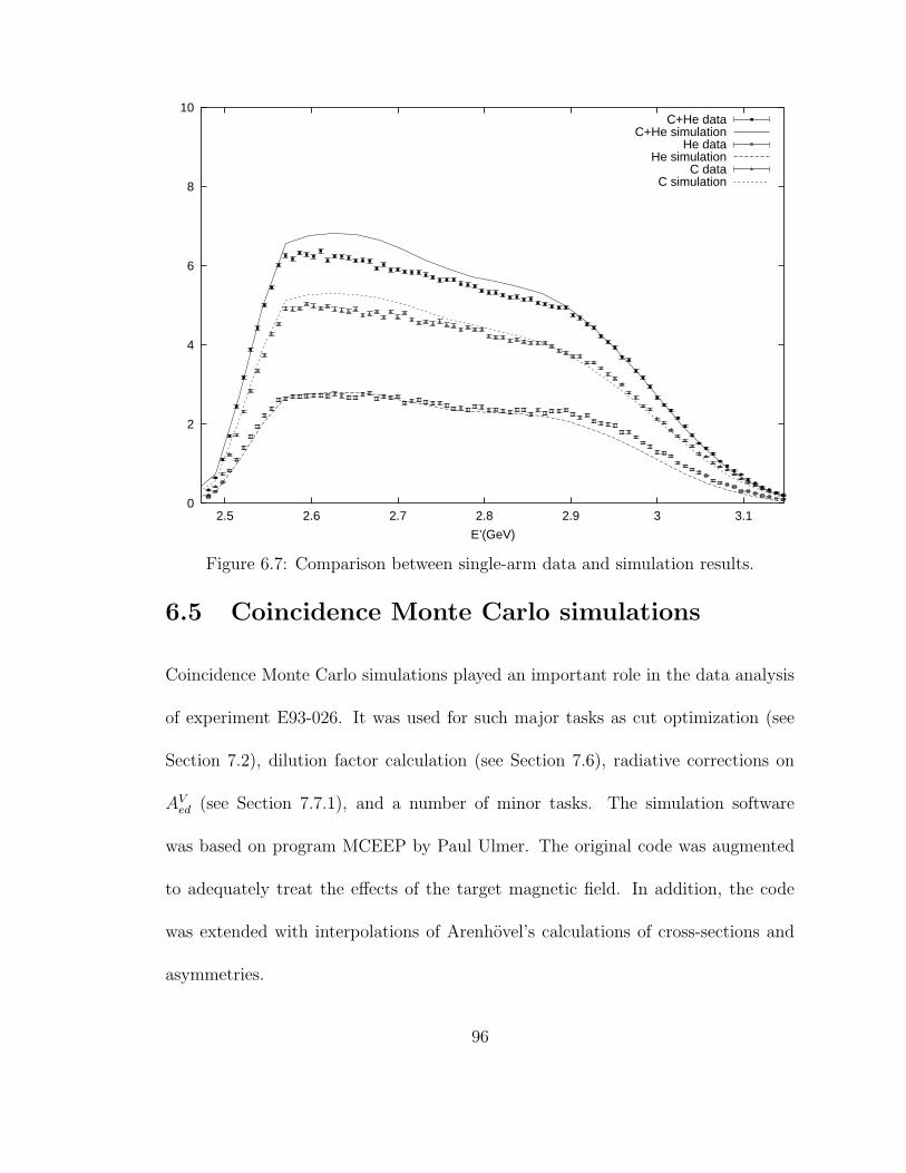
0
2
4
6
8
10
2.5 2.6 2.7 2.8 2.9 3 3.1
E’(GeV)
C+He dataC+He simulation
He dataHe simulation
C dataC simulation
Figure 6.7: Comparison between single-arm data and simulation results.
6.5 Coincidence Monte Carlo simulations
Coincidence Monte Carlo simulations played an important role in the data analysis
of experiment E93-026. It was used for such major tasks as cut optimization (see
Section 7.2), dilution factor calculation (see Section 7.6), radiative corrections on
AVed (see Section 7.7.1), and a number of minor tasks. The simulation software
was based on program MCEEP by Paul Ulmer. The original code was augmented
to adequately treat the effects of the target magnetic field. In addition, the code
was extended with interpolations of Arenhovel’s calculations of cross-sections and
asymmetries.
96

6.5.1 Basics of MCEEP
The program allows a user to choose one of the three options: elastic scattering,
bound final state or unrestricted continuum. For the bound state case the ejectile
momentum is calculated from the bound state missing mass specified in the input
file, whereas for the continuum case it is randomly sampled and the missing mass is
calculated on an event-by-event basis.
Sampled quantities
The program samples the experimental acceptance uniformly, using calculated cross-
sections as weighting factors when simulating realistic physical spectra. In a most
general case (continuum scattering) an event is generated by “throwing” seven ran-
dom quantities: the in-plane and out-of plane angles and momenta for the electron
and the hadron, and the energy of the bremsstrahlung photon, radiated either before
or after the main interaction depending on the “coin toss”.
For the bound final state, the hadron momentum is calculated from other
quantities. For elastic scattering, only electron angles are sampled, and all other
quantities are calculated.
HMS spectrometer model
Simulation of event detection in the HMS consisted of two major parts: forward
tracking of the incident particle through the target magnetic field and HMS magnets
97
and reconstruction of the successful event. To account for the effect of the beam
rastering, the vertex coordinates were randomly sampled within the raster spot.
The standard (i.e. without the target field and beam raster corrections) part
of the algorithm consisted of the following basic steps:
1) projecting a particle to the magnet aperture, assuming motion along a
straight line;
2) checking the coordinates of the particle versus the aperture of the magnet;
if they fall outside the actual dimensions of the magnet aperture then the particle
is labeled as stopped, and the algorithm proceeds to the next iteration;
3) tracking the particle forward in the magnetic field of the spectrometer mag-
net using COSY Infinity coefficients.
These steps are repeated for each of the 4 HMS magnets. Finally, if the
particle does not stop in one of the magnets, the same approach is used to find
which detectors (assumed to be 100% efficient) are fired in the HMS detector hut,
and the 4 focal plane quantities are determined.
The reconstruction algorithm essentially repeats that of the data analysis code
(see Subsection 6.3.1).
Cross sections
The cross sections are calculated assuming plane wave impulse approximation (PWIA),
i.e. the virtual photon is absorbed by one off-shell nucleon which (as well as the
98

incident electron) can be described by a plane wave. Under these conditions the
(e, e′N) cross section can be factorized as follows [2]:
dσ
dεfdΩedεNdΩN
= KσeNS(Em, ~pm), (6.22)
where K is a kinematic factor, σeN is the elementary off-shell electron-nucleon scat-
tering cross-section and S(Em, ~pm) is the spectral function which represents the
probability of finding a nucleon with initial momentum ~pm and binding energy Em
within the nucleus. The elementary cross-section σeN is calculated using the “cc1”
prescription of de Forest [68]:
σeN = σMott
[
Q4
q4WC + (tan2 θ/2− Q2
q2)WT−
−Q2
q2
(
tan2 θ/2− Q2
q2
)1/2
WI cosφ+
(
tan2 θ/2− Q2
q2 cos2 φ
)
WS
]
(6.23)
WC =1
4EE ′
[
(E + E ′)2(
F 21 +q2µ
4M2κ2F 22
)
− q2(F1 + κF 2)2]
(6.24)
WT =qµ2
2EE ′ (F1 + κF2)2 (6.25)
WS =p′2 sin2 γ
EE ′
(
F 21 +q2µ
4M2κ2F 22
)
(6.26)
WI = −p′2 sin2 γ
EE ′ (E − E ′)
(
F 21 +q2µ
4M2κ2F 22
)
, (6.27)
99
where E and E ′ are the initial (off-shell) and final energies of the struck nucleon, p′
is the momentum of the struck nucleon, γ is the angle between ~p′ and ~q, qµ is the
four-momentum transfer corrected for off-shell effects, and F1 and F2 are Dirac and
Pauli form factors.
Spectral functions
The MCEEP has many built-in spectral functions. Additionally, the modular struc-
ture of MCEEP allows various spectral functions representing different models of
the nuclei to be easily incorporated into the program through external files.
The simulations for 4He used a parametrization for t+p breakup channel using
Urbana potential [69] (MCEEP option 32). The nitrogen spectral function was
approximated by that of 16O for 1p1/2, 1p3/2 and 1s1/2 shells (MCEEP options 40,
41 and 42). The spectral function for aluminum was a custom parametrization based
on quasielastic data. Finally, copper and nickel were approximated by the carbon
spectral function provided by I. Sick.
Radiative effects
The MCEEP has options for simulating internal and external radiation and ioniza-
tion energy loss. Radiative effects are only taken into account for electrons 8 by
sampling bremsstrahlung photon energy. The peaking approximation is used, i.e.
the photon is emitted either along the incident electron momentum or along the
8Those of hadrons are negligible due to their high mass.
100
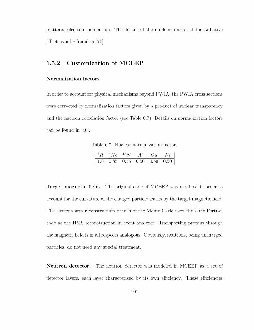
scattered electron momentum. The details of the implementation of the radiative
effects can be found in [70].
6.5.2 Customization of MCEEP
Normalization factors
In order to account for physical mechanisms beyond PWIA, the PWIA cross sections
were corrected by normalization factors given by a product of nuclear transparency
and the nucleon correlation factor (see Table 6.7). Details on normalization factors
can be found in [40].
Table 6.7: Nuclear normalization factors
2H 4He 15N Al Cu Ni1.0 0.85 0.55 0.50 0.50 0.50
Target magnetic field. The original code of MCEEP was modified in order to
account for the curvature of the charged particle tracks by the target magnetic field.
The electron arm reconstruction branch of the Monte Carlo used the same Fortran
code as the HMS reconstruction in event analyzer. Transporting protons through
the magnetic field is in all respects analogous. Obviously, neutrons, being uncharged
particles, do not need any special treatment.
Neutron detector. The neutron detector was modeled in MCEEP as a set of
detector layers, each layer characterized by its own efficiency. These efficiencies
101

were calculated following the procedure by Madey et al. [71]. The probability of
firing the n-th plane of the neutron detector was calculated based on individual
plane efficiencies (see Table 6.8).
Table 6.8: Modeled neutron detection efficiencies by detector plane
1 2 3 4 5 60.095 0.095 0.154 0.143 0.116 0.116
The finite timing resolution for the neutron detector was simulated by Gaus-
sian smearing of the hit position.
Arenhovel’s calculations. Even though MCEEP is capable of calculating po-
larization observables, for a precision measurement of GnE one needs to use full cal-
culations including the effects of the meson exchange currents, isobar configurations
and other relevant physical processes. Additionally, it is desirable to have accurate
calculations for the deuteron scattering cross section as well to minimize the uncer-
tainty in the dilution factors. Such calculations were provided by H. Arenhovel on a
kinematical grid 9 shown in Table 6.9. The values of cross sections and asymmetries
between the grid points were obtained by spline interpolation.
The D(e, e′N) scattering cross-section was radiated by multiplying by a radia-
tive correction factor calculated from other materials. The AVed was calculated for
each event and written out to the output ntuple, thus simplifying the procedure of
experimental acceptance averaging.
9Note that the grid in θcmnp has two step sizes. The step size is 2.5 in the quasi-elastic region
(0 − 30 and 150 − 180) and 5 elsewhere.
102
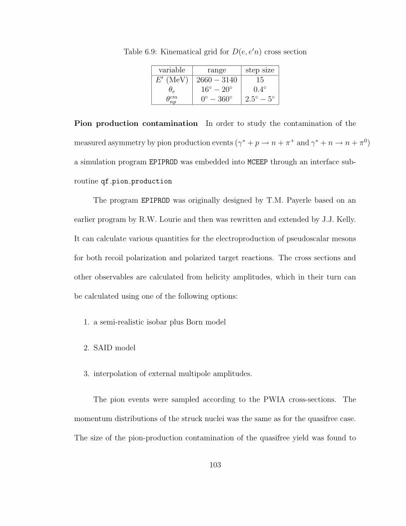
Table 6.9: Kinematical grid for D(e, e′n) cross section
variable range step sizeE ′ (MeV) 2660− 3140 15
θe 16 − 20 0.4
θcmnp 0 − 360 2.5 − 5
Pion production contamination In order to study the contamination of the
measured asymmetry by pion production events (γ∗ + p→ n+ π+ and γ∗ + n→ n+ π0)
a simulation program EPIPROD was embedded into MCEEP through an interface sub-
routine qf pion production
The program EPIPROD was originally designed by T.M. Payerle based on an
earlier program by R.W. Lourie and then was rewritten and extended by J.J. Kelly.
It can calculate various quantities for the electroproduction of pseudoscalar mesons
for both recoil polarization and polarized target reactions. The cross sections and
other observables are calculated from helicity amplitudes, which in their turn can
be calculated using one of the following options:
1. a semi-realistic isobar plus Born model
2. SAID model
3. interpolation of external multipole amplitudes.
The pion events were sampled according to the PWIA cross-sections. The
momentum distributions of the struck nuclei was the same as for the quasifree case.
The size of the pion-production contamination of the quasifree yield was found to
103
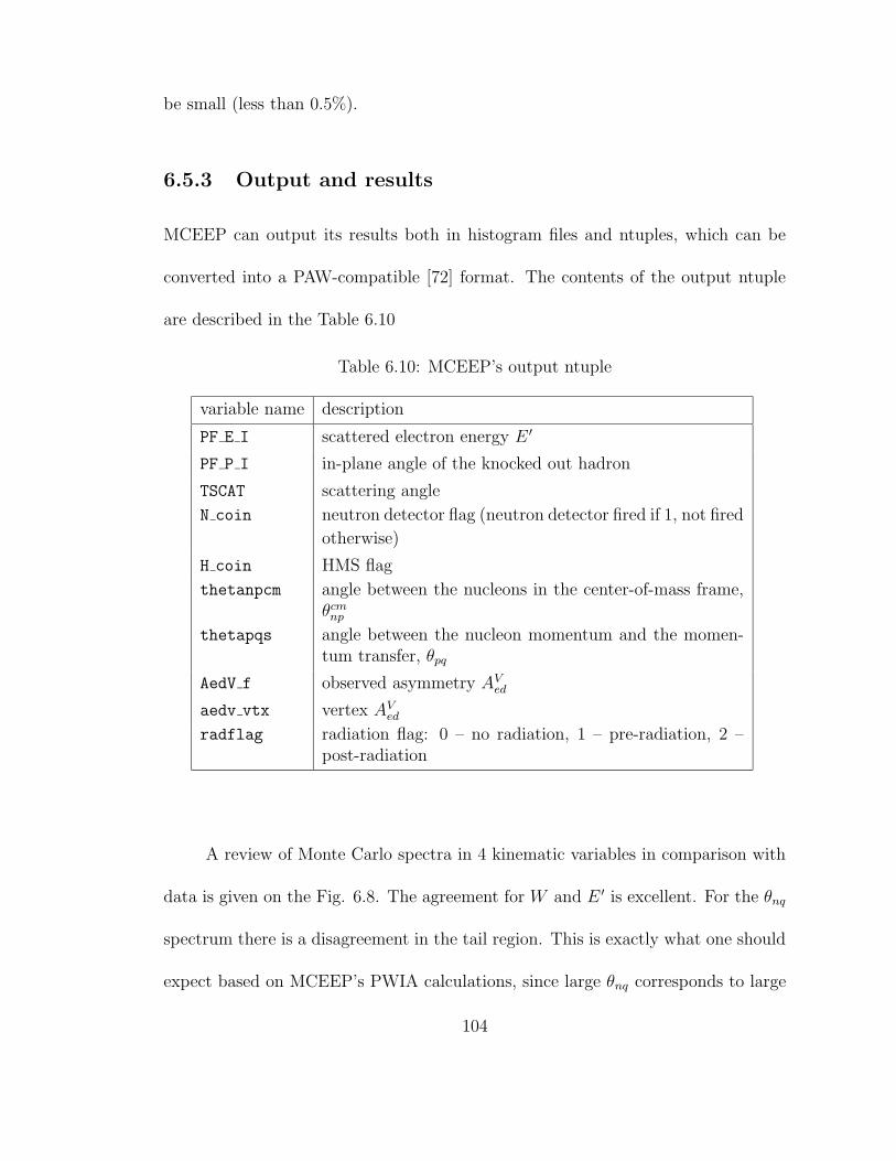
be small (less than 0.5%).
6.5.3 Output and results
MCEEP can output its results both in histogram files and ntuples, which can be
converted into a PAW-compatible [72] format. The contents of the output ntuple
are described in the Table 6.10
Table 6.10: MCEEP’s output ntuple
variable name description
PF E I scattered electron energy E ′
PF P I in-plane angle of the knocked out hadron
TSCAT scattering angle
N coin neutron detector flag (neutron detector fired if 1, not fired
otherwise)
H coin HMS flag
thetanpcm angle between the nucleons in the center-of-mass frame,θcmnp
thetapqs angle between the nucleon momentum and the momen-tum transfer, θpq
AedV f observed asymmetry AVed
aedv vtx vertex AVed
radflag radiation flag: 0 – no radiation, 1 – pre-radiation, 2 –post-radiation
A review of Monte Carlo spectra in 4 kinematic variables in comparison with
data is given on the Fig. 6.8. The agreement for W and E ′ is excellent. For the θnq
spectrum there is a disagreement in the tail region. This is exactly what one should
expect based on MCEEP’s PWIA calculations, since large θnq corresponds to large
104
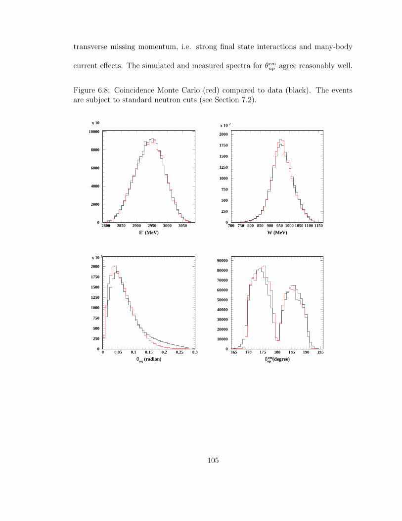
transverse missing momentum, i.e. strong final state interactions and many-body
current effects. The simulated and measured spectra for θcmnp agree reasonably well.
Figure 6.8: Coincidence Monte Carlo (red) compared to data (black). The eventsare subject to standard neutron cuts (see Section 7.2).
E′ (MeV)
0
2000
4000
6000
8000
10000
x 10
2800 2850 2900 2950 3000 3050
W (MeV)
0
250
500
750
1000
1250
1500
1750
2000
x 10 2
700 750 800 850 900 950 1000 1050 1100 1150
θnq (radian)
0
250
500
750
1000
1250
1500
1750
2000
x 10 2
0 0.05 0.1 0.15 0.2 0.25 0.3
θnpcm (degree)
0
10000
20000
30000
40000
50000
60000
70000
80000
90000
165 170 175 180 185 190 195
105
Chapter 7
Data analysis
This chapter deals with the details of the experimental data analysis. The chapter
starts with a description of the data replay process. Then we discuss cuts and inputs
(target and beam polarizations) used in asymmetry calculation. Then we proceed
to packing fraction and dilution factor calculations. The last two sections of the
chapter discuss various corrections applied to the calculated asymmetry and the
GnE extraction procedure.
7.1 Data replay
Data replay reconstructs particle tracks and event kinematics from TDC and ADC
signals stored in the CODA format. This task is handled by the event analyzer
described in the previous chapter. Since the entire experimental data set consists of
hundreds of runs, the replay was done in parallel on an autonomous computer system
called Batch Farm. The submission and control of analysis jobs was conducted by
a Tcl/Tk script package “BatchMan” (for “Batch Manager”).
106

The initial stage of data replay involves two steps: selection of runs to be
analyzed and preparation of input for the event analyzer (detector calibrations).
7.1.1 Runs selection
Along with data taken under normal running conditions with the polarized target,
other data were taken in the experiment for different purposes (tests of experimental
hardware, calibration data, beam polarization measurements etc.). Also, some of
the production data were damaged because of various problems experienced during
the data taking. These runs must be excluded from the analysis process. A more
detailed list of excluded runs is given below:
• non-15ND3 targets (carbon, empty, hole)
• Møller runs
• checkup runs
• DAQ crash during the run
• serious hardware problems (magnet quenches, persistent HV trips etc.)
• unstable helium level in the target nose
• sudden loss of target polarization
• wrong position of the HMS collimator.
107
7.1.2 Detector calibrations
Raw data files contain information about particle tracks in the form of ADC and
TDC signals of detector hits. In order to reconstruct the tracks and calculate phys-
ical quantities of interest, one needs to match the timing of individual detectors,
supply conversion constants between ADCs and energy deposited in a detector etc.,
i.e. to perform detector calibrations.
HMS calibrations
HMS calibrations consist of timing calibrations of hodoscopes, generating time-to-
distance maps for the drift chambers, and determining gains of each block of the
lead glass calorimeter. Since the HMS is a standard piece of equipment of TJNAF
Hall C, these calibrations are a well-established procedure, the details of which can
be found elsewhere [56].
Neutron detector timing calibrations
Signals from PMT of detector scintillators arrive at the counting room with a
delay of a few tens or even hundreds of nanoseconds. Due to unequal cable lengths,
intrinsic transit times and high voltages, these delays generally differ between right
and left PMTs. For a precise calculation of hit positions and meantime associated
with a track it is necessary to apply time offset corrections to the meantime and
TDC difference of a hit. These offsets are calculated by fitting the corresponding
spectra of individual detectors. The offset is then given by the peak position. After
108

the calibration is completed, offset parameters are written to text files which are
later read in by the analyzer. The quality of the calibration can be checked by
plotting TDC difference and meantime spectra for individual detectors and making
sure that they are centered around zero.
Neutron detector energy calibration
Energy calibrations of the neutron detector were performed using cosmic data.
Cosmic rays are dominated by high energy muons, for which the energy deposited
in a given amount of material is well known [40] (e.g 22 MeV for 10 cm scintilla-
tors). Thus the position of the cosmic peak provides the desired conversion constant
between the ADC channels and energy.
7.1.3 Replay procedure
The replay of large amounts of data was performed using the Jefferson Lab comput-
ing facility (Batch Farm). The Batch Farm consists of 175 Linux CPUs. A user can
submit a job to the Batch Farm by means of a command file which contains basic
information about the command to be executed, input files and relevant parameters.
An interface between the Batch Farm and a user was provided by a Tcl/Tk
package “BatchMan” , custom designed for experiment E93-026. It allows a user
to observe the status of submitted jobs, kill undesired jobs, restart failed jobs and
submit new jobs.
When a list of runs is submitted for analysis, BatchMan creates a command
109
file for each run and submits it to the Batch Farm. The command file contains a
reference to the batch job script which copies analysis setup and the first segment
of the raw data 1 to the local Batch Farm computer and launches the analysis job.
While a data segment is being analyzed, the next one is copied to the local disk
drive in a background process. Upon completion of the analysis job the batch job
script copies the results to BatchMan output directories.
7.2 Cut optimization
For the purpose of GnE extraction we only need quasielastic ~d(~e, e′n) events. Co-
incidence ntuples produced by the event analyzer contain all events that fired an
HMS trigger and were successfully processed by DAQ (including inelastic, acciden-
tal background and proton events). Therefore, one needs to select desired events
by applying cuts. One cut is obvious: if we are interested in neutron events, we
need to look at events with the neutron PID (PID codes 11, 12, 13, 14 and 15).
The other cuts are determined by figure-of-merit considerations and the quality of
Monte-Carlo model in a given kinematic region.
The figure-of-merit is affected by kinematic cuts through the dilution factor:
cuts emphasizing the quasielastic region improve the dilution factor and thus reduce
the error magnification factor. At the same time, these cuts inevitably reduce the
number of good events, too, and thus increase the statistical error itself. The op-
1Due to size limitations on the tape servers raw data files are split into 2 Gb segments. Thenumber of segment files per run varied from 1 to 4 for E93-026.
110

timum can be determined with the use of Monte Carlo simulations. The results of
simulations are shown in Figure 7.1. The figure shows figure of merit as a function
of kinematic variables for several distinct sets of cuts. The figure of merit can be
defined as the experimental time required for achieving given accuracy, and for fixed
PB and PT it is proportional to f√R, where f is the dilution factor and R is the
event rate.
W
f*sq
rt(R
)
ypos=30
θnq=0.06θnq=0.07θnq=0.08θnq=0.09θnq=0.10θnq=0.11
W
f*sq
rt(R
)
ypos=40
W
f*sq
rt(R
)
ypos=50
W
f*sq
rt(R
)
W
f*sq
rt(R
)
ypos=60
W
f*sq
rt(R
)0.6
0.62
0.64
0.66
0.68
0.7
60 80 100 120
0.66
0.68
0.7
0.72
0.74
0.76
60 80 100 120
0.7
0.72
0.74
0.76
0.78
0.8
60 80 100 1200.7
0.72
0.74
0.76
0.78
0.8
0.82
60 80 100 120
Figure 7.1: Figure of merit for different kinematic cuts. Note that W (MeV) here isnot the invariant mass, but rather W0, the width of the cut on the invariant mass:|W − 939| < W0.
111

Table 7.1: ~d(~e, e′n) cuts. Here ypos is the horizontal position of the neutron track atthe reference plane (plane 3 of the neutron detector), Etrack is the energy depositedin the neutron detector, ∆t is coincidence time, ZBEAM is the coordinate of thevertex along the beam direction (zero corresponds to the center of the target cell)and MN = 939 MeV is the nucleon mass.
cut suppressed eventsNphotoelectrons > 2 pions in the HMS|W −MN | < 70 MeV inelastics (∆ electroproduction)
E ′ > 2829 MeV same as above|ypos| < 40 cm heavy nuclei (broad Fermi distribution)θpq < 0.08 rad high missing momentum−3 < ∆t < 5 ns accidentalsEtrack > 12 MeV low-energy noise in the neutron detector|ZBEAM | < 3.2 cm events reconstructed outside the target cellθe > 0.26 rad events reconstructed outside spectrometer acceptance
As one can see, the figure-of-merit (FOM) generally favors wide-open cuts
rather than tight ones: it increases monotonically with the width of the W cut, the
widest ypos cuts also give highest FOM, and finally, the three wide θnq cuts all lie
higher than the tight θnq cuts. However, in all cases the dependence is fairly flat
which allows us a certain freedom of choice. This freedom was used to pick cuts
emphasizing the kinematic region where Monte Carlo works best. Some events do
not have an adequate model in Monte Carlo (e.g. pions in HMS, background etc.).
The cuts for reduction of these events were developed using qualitative reasoning
and a trial-and-error approach. A complete set of cuts used in the analysis is given
in Table 7.1.
112

7.3 Target polarization
The target DAQ permits online monitoring of the target polarization. The prompt
availability of the results comes at the expense of the accuracy of the measurement.
The quality of online target polarizations is sufficient for data-taking purposes, but
the actual physical calculations are more demanding.
Therefore, upon the completion of the experiment a full offline analysis of
NMR signals was performed, including reevaluation of baselines, refitting the NMR
signals and reanalysis of TE measurements.
7.3.1 Baseline subtraction
A baseline is the response of the NMR circuit in the absence of target polariza-
tion. Baseline measurements (normally taken after each anneal) were performed by
changing the target magnetic field such that the NMR signal of the deuteron was
pushed outside the frequency sweep range. Baselines and NMR signals were stored
separately in Labview binary files so that in case of a noisy or corrupt baseline a
different one could be associated with a given set of NMR signals.
The presence of the polarization signal introduces a slight distortion of the
NMR circuit response. Additionally, temperature fluctuations and beam distur-
bance can also affect the shape of the NMR signal. Therefore, baseline subtraction
is followed by a fit of the quadratic polynomial to the “wings” of the subtracted
113

signal with subsequent subtraction2. The analyzed NMR signal on different stages
of the offline analysis is shown in Figure 7.2. Note that the second and the third
plots are almost identical, which is due to the fact that the wings are normally very
small and the constant pedestal subtraction suffices in most cases.
Figure 7.2: NMR signal on different stages of the offline analysis.
114

Figure 7.3: TE calibration constants for various groups. The ±σ for the groupsare shown with horizontal solid lines. The symbols are: plus – stick 1 top, asterisk– stick 1 bottom, circle – stick 2 top, x – stick 2 bottom, triangle – stick 3 top,diamond – stick 3 bottom, puff – stick 4 top, cross-hair – stick 4 bottom.
7.3.2 TE constants
If a material is allowed to thermalize, the spin temperature becomes equal to the
actual (“lattice”) temperature. Under these conditions the target polarization is
completely determined by the magnetic field, temperature and the magnetic moment
of the deuteron and can be calculated analytically (See Eq. A.2). The area under
2In practice, this is done in two steps: first a constant pedestal is subtracted from the signal andthen one fits the residual wings with a quadratic polynomial. This approach permits to improvethe quality of the fit.
115

Table 7.2: Target polarization uncertainties.stick 3 top 3.30%stick 3 bottom 4.61%stick 4 top 4.90%stick 4 bottom 5.24%
the NMR signal measured in thermal equilibrium (a TE constant) thus provides the
calibration constant for the NMR measurement.
Since the target polarization in thermal equilibrium is hundreds of times
smaller than the typical polarization during production running, performing TE
calibrations is a challenging task. All 110 TE measurements taken during E-93026
were carefully examined. Excluding unacceptable measurements (noisy signals, non-
thermalized material, etc.) resulted in the total of 2095 good signals with from 12
to 36 signals in one TE measurement. Good signals were averaged for each material.
These group averages were used in the actual target polarization calculations.
The uncertainty on target polarization was estimated by scatter of TE con-
stants (see Table 7.2). The TE constants normalized to group averages are shown
in Figure 7.3.
7.4 Beam polarization
The beam polarization was measured in a series of Møller runs. Individual measure-
ments were combined into groups defined by changes in the half-wave plate positions.
It has been assumed that the variation of the beam polarization values with time
116
was linear, and thus the values of beam polarization for runs between Møller mea-
surements were obtained by linear fits. The details of individual measurements are
given in Appendix A.2
7.4.1 Hall A current leakage
The Jefferson Lab accelerator provides the electron beam with (generally) different
energies and/or polarizations to three experimental Halls. This is achieved either
by using one laser for all three Halls or using one laser per each Hall. For the
Q2 = 1.0 (GeV/c)2 data, the latter was the case.
When running on three different lasers, it is possible for the current of other
halls to leak into Hall C slits. Since Hall B was run in a high-polarization, low-
current mode, the leakage from that Hall was of no concern. The case was the
opposite with the Hall A (high current, low polarization), resulting in a sizable
admixture of low-polarized Hall A beam in the Hall C beam.
The leakage was measured in a procedure that involved measuring the beam
current with:
A. C slit open, C laser off, A laser on
B. C slit closed
C. C slit open, both A and C lasers on.
117

The HMS scaler was used as a luminosity monitor. The leakage is given by
Ileakage =A−BC −B ,
where A, B, C is the HMS scaler rate for each of the three steps.
The Hall A current leakage was normally measured every shift (i.e. every 8
hours). After a short bad period (with leakages up to 9%) the leakage was kept
within 2%. Since the Hall A polarization is of the same sign and about half size of
that of the Hall C, the resulting correction is less then 1%. Taking into consideration
other dominant errors and the statistical accuracy of the experiment, it has been
decided to neglect this correction. Instead, a 1% uncertainty was added to the beam
polarization error.
7.4.2 Results
The results of the Møller measurements and their parameterizations using straight
line fits is given in Figure 7.4. The global average of the beam polarization was
found to be 71.8± 2.4%
A breakdown of the total beam polarization error by source is given in Ta-
ble 7.3. The error is dominated by scatter in beam polarization values.
118
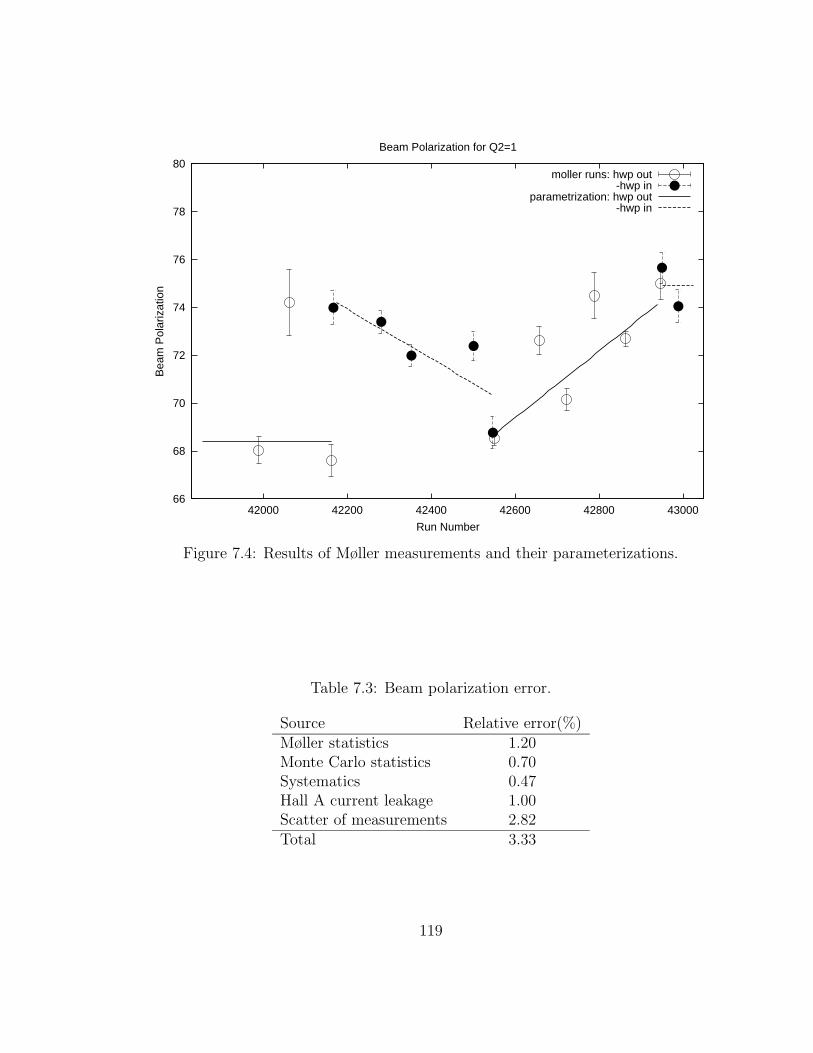
66
68
70
72
74
76
78
80
42000 42200 42400 42600 42800 43000
Bea
m P
olar
izat
ion
Run Number
Beam Polarization for Q2=1
moller runs: hwp out-hwp in
parametrization: hwp out-hwp in
Figure 7.4: Results of Møller measurements and their parameterizations.
Table 7.3: Beam polarization error.
Source Relative error(%)Møller statistics 1.20Monte Carlo statistics 0.70Systematics 0.47Hall A current leakage 1.00Scatter of measurements 2.82Total 3.33
119
7.5 Packing fraction
The packing fraction of the polarized target is the ratio of the volumes (or thick-
nesses, if the distribution of materials over the target face is uniform) of polarized
material and cryogenic helium inside the target cup as seen by the beam. This quan-
tity determines dilution of the measured asymmetry by unpolarized helium inside
the target, which together with contributions from other material determines the
overall dilution factor f .
7.5.1 Method of determination
Unlike other target materials, the thickness of internal helium cannot be measured
directly, since the frozen ammonia has the form of small beads and does not fill up
the volume of the target cell uniformly. Further, the packing fraction of a target
changes during the data acquisition due to material leakage, target anneals, changes
in the beam-target alignment etc. Therefore, one obtains the packing fraction using
the observed event rates. One can simulate inclusive event rates for targets with
different packing fractions with the inclusive simulation program described in the
previous chapter, and then extract the actual packing fraction by comparing the
results of the simulations with the measured rates.
The inclusive event rate from a target material is essentially the product of
the cross section and luminosity integrated over the experimental acceptance. The
total rate is the sum of rates from all target layers. Since for each layer the rate is
120

approximately proportional to the thickness of the layer 3, the relation between the
total inclusive rate and the packing fraction is approximately linear:
p.f. = offset + rate× slope. (7.1)
Hence, one needs to perform simulations for two values of packing fraction in
order to determine the offset and slope of Equation 7.1. It is convenient to choose
the two reference values of the packing fraction to be 40% and 60%. Additionally,
to avoid a systematic uncertainty related to absolute normalization we normalize
ND3 rate by carbon rate. The packing fraction is obtained by linear interpolation:
p.f. =(r − r40)40 + (r60 − r)60
r60 − r40%, (7.2)
where r is the ratio of the 15ND3 rate to carbon rate as measured in data, and r40
and r60 are model ratios assuming packing fraction of 40% and 60%, correspondingly.
7.5.2 Event selection
The data were cut on the number of Cerenkov photoelectrons (hcer npe > 2) for
pion rejection. Both Monte Carlo and data were also cut on the scattered electron
energy (2880 < E ′ < 3100 MeV) to emphasize the quasielastic kinematics. The
stick 3 data were additionally cut on the horizontal raster position (beamx > 0) to
3There are nonlinear effects due to thickness-dependent radiative energy losses. However, theyare of the order of 1% and can be neglected here.
121

eliminate the contribution from the side wall (see Section 7.6.3 for details).
7.5.3 Procedure and results
The calculation of the packing fraction was performed separately for two different
target inserts with different material loads (“stick 3” and “stick 4”). For each insert,
the entire set of 15ND3 and carbon data was replayed in the single-arm mode
of the analyzer (with the neutron detector side ignored). Then a cut processor
counted events that survived the imposed cuts 4. The inclusive event rate was
normalized by dead-time corrected charge (provided by syncfilter output), HMS
trigger efficiency, and the tracking efficiency. Finally, the 15ND3/carbon rate ratio
was formed.
The data ratio was compared to simulated 5 ratios with packing fraction of
40% and 60%. The ratios are shown in Figure 7.5(a). As one can see, the shapes
of the E ′-dependences for different packing fractions are practically identical, which
confirms that nonlinear effects due to radiation are small.
The packing fraction was extracted from these ratios using Equation 7.2. The
scatter of the packing fraction values over E ′ characterizes systematic and statistical
accuracy of the measurement. The statistically weighted average over all E ′ bins
was taken as the final result for the packing fraction. The systematic error contained
two contributions (added in quadrature): scatter in E ′ bins (3.2% for both sticks)
4The events were counted in 32 uniform E ′ bins, covering range from 2660 MeV to 3140 MeV,to study the systematic errors.
5see Section 6.4 for a description of the simulation package
122
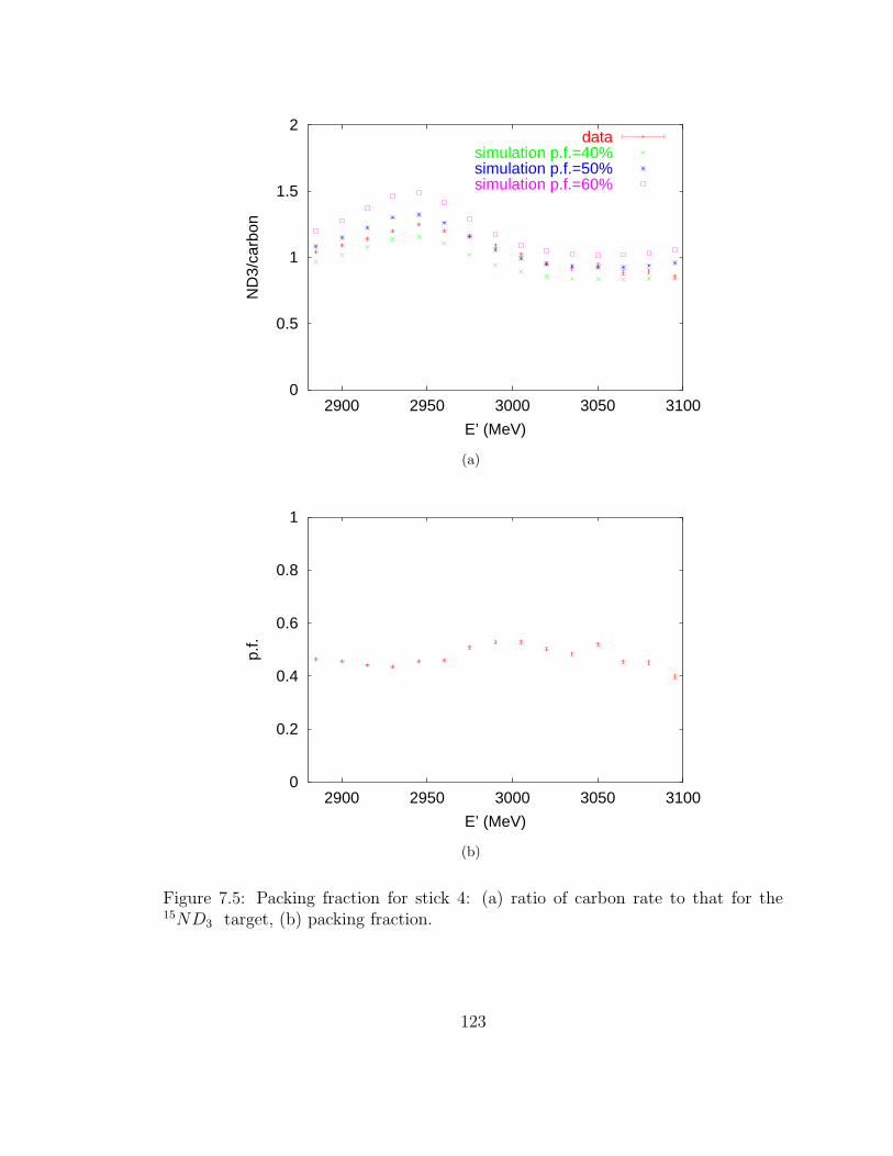
0
0.5
1
1.5
2
2900 2950 3000 3050 3100
ND
3/ca
rbon
E’ (MeV)
datasimulation p.f.=40%simulation p.f.=50%simulation p.f.=60%
(a)
0
0.2
0.4
0.6
0.8
1
2900 2950 3000 3050 3100
p.f.
E’ (MeV)
(b)
Figure 7.5: Packing fraction for stick 4: (a) ratio of carbon rate to that for the15ND3 target, (b) packing fraction.
123
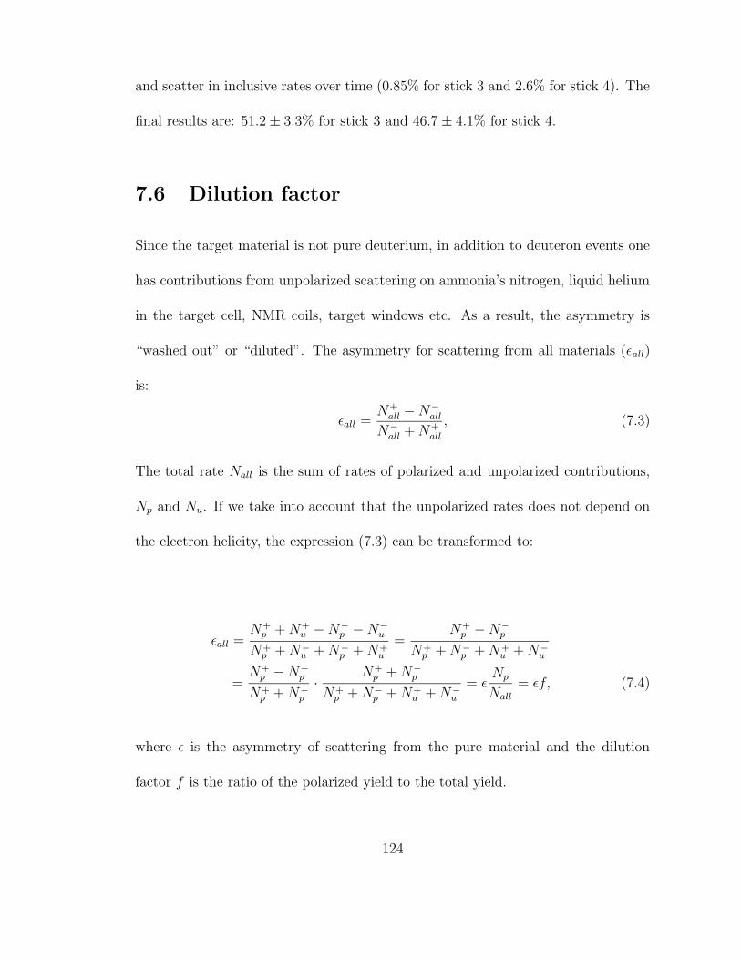
and scatter in inclusive rates over time (0.85% for stick 3 and 2.6% for stick 4). The
final results are: 51.2± 3.3% for stick 3 and 46.7± 4.1% for stick 4.
7.6 Dilution factor
Since the target material is not pure deuterium, in addition to deuteron events one
has contributions from unpolarized scattering on ammonia’s nitrogen, liquid helium
in the target cell, NMR coils, target windows etc. As a result, the asymmetry is
“washed out” or “diluted”. The asymmetry for scattering from all materials (εall)
is:
εall =N+
all −N−all
N−all +N+
all
, (7.3)
The total rate Nall is the sum of rates of polarized and unpolarized contributions,
Np and Nu. If we take into account that the unpolarized rates does not depend on
the electron helicity, the expression (7.3) can be transformed to:
εall =N+
p +N+u −N−
p −N−u
N+p +N−
u +N−p +N+
u
=N+
p −N−p
N+p +N−
p +N+u +N−
u
=N+
p −N−p
N+p +N−
p
·N+
p +N−p
N+p +N−
p +N+u +N−
u
= εNp
Nall
= εf, (7.4)
where ε is the asymmetry of scattering from the pure material and the dilution
factor f is the ratio of the polarized yield to the total yield.
124

For the purposes of our experiment it is convenient to express polarized and
unpolarized yields of the Equation 7.4 via rates of specific target materials. The
only polarized material in the target is the deuterium6 and thus Np = Nd. The
unpolarized yield can be broken into contributions from the ammonia nitrogen NN ,
helium inside the target cell N intHe , helium outside the target cell N ext
He and target walls
NW . Since the relative ratio of ammonia and internal helium yields is determined
by the packing fraction, we can rewrite (7.4) as:
f =Nd p.f.
N extHe +Nd p.f.+NNp.f.+N int
He(1− p.f.), (7.5)
where the yields for materials inside the target cell are calculated assuming that
they fill up its entire volume.
Since yields are determined by kinematic-dependent scattering cross sections,
the dilution factor is also a function of kinematic variables. The coincidence event
rate measured in the experiment cannot be separated into contributions from specific
materials. Therefore, for a proper determination of the experimental dilution factor
one needs to run Monte Carlo simulations.
The simulations were performed using the customized version of MCEEP (see
Section 6.5). The simulation was run separately for sticks 3 and 4 because of their
different material thicknesses (due to different packing fractions and different orien-
tation with respect to the beam).
6In reality, the nitrogen also carries some polarization, but it does not contribute to the neutronasymmetry. See page 49.
125

7.6.1 Pion contamination
In electron-nucleon scattering the virtual photon may excite the nucleon to a res-
onant state which then decays into a nucleon with an emission of a pion. Such
reaction mechanism is known as pion electroproduction. For a coincidence electron-
neutron measurement only two such reactions are of interest: γ∗ + p→ n+ π+ and
γ∗ + n→ n+ π0.
Most of events coming from these reaction are suppressed by kinematic cuts,
in particular by the cut on the invariant mass, |W − MN | < 70 MeV, where
MN = 939 MeV is the nucleon mass. However, some of pion events because of Fermi
broadening may have kinematics similar to that of the quasielastic scattering and
thus contaminate the measured asymmetry. It has been experimentally verified that
these events do not carry any statistically significant asymmetry. Therefore, their
contribution (found to be 0.44%) can be included into the dilution factor calculation.
7.6.2 Misorientation of the 4K shield
In the beginning of the data analysis it has been found that the distribution of the
events along the beam direction has strange shoulders outside the target cup (see
Figure 7.6) at |ZBEAM | > 3 cm . It has been established that these shoulders were
due to a misorientation of the 4K shield (which surrounds the tailpiece with the
target insert) such that for some raster positions the beam was coming not through
the thin window in the shield, but rather through the shield itself, thus transversing
126

an order of magnitude larger amount of material than expected (see Figure 7.7).
A Geant 4 simulation (see below for details) showed that the effective thickness of
the 4K shield was 1.822 mm for stick 3 and 1.874 mm for stick 4. The majority of
these events were eliminated by the standard analysis cut |ZBEAM < 3.2 cm|. The
residual contribution from the 4K shield events was estimated by fitting a sum of
three asymmetric Gaussians to the ZBEAM spectrum (see Figure 7.6) and was found
to be 0.23%± 0.05%. This correction was applied to the dilution factor.
7.6.3 Stick 3 rotation
When stick 3 was extracted, we found that the radiation damage pattern on the
material was consistent with an anomalous counter-clockwise rotation of the insert
about the vertical axis. Obviously, such a rotation affects the thicknesses of the
material transversed by the beam and therefore the dilution factor. In order to
account for this effect, a C++ program was written based on Geant 4 libraries [52].
The program calculates average thickness of each target material in the beam’s
path and incorporates horizontal and vertical displacement and a rotation about
the vertical axis of the target insert.
The angle of the stick rotation was determined by the 4 mm horizontal dis-
placement of the hole target to be 15.8. However, since the raster calibrations are
only accurate to about 1 mm, there is a 3.8 uncertainty in the rotation angle.
The mutual arrangement of the beam and the rotated stick is shown in Fig-
127
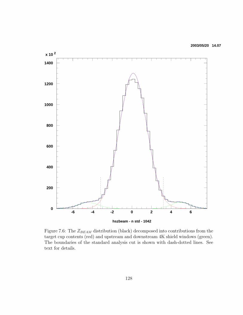
hszbeam - n std - 1042
0
200
400
600
800
1000
1200
1400
x 10 2
-6 -4 -2 0 2 4 6
2003/05/20 14.07
Figure 7.6: The ZBEAM distribution (black) decomposed into contributions from thetarget cup contents (red) and upstream and downstream 4K shield windows (green).The boundaries of the standard analysis cut is shown with dash-dotted lines. Seetext for details.
128
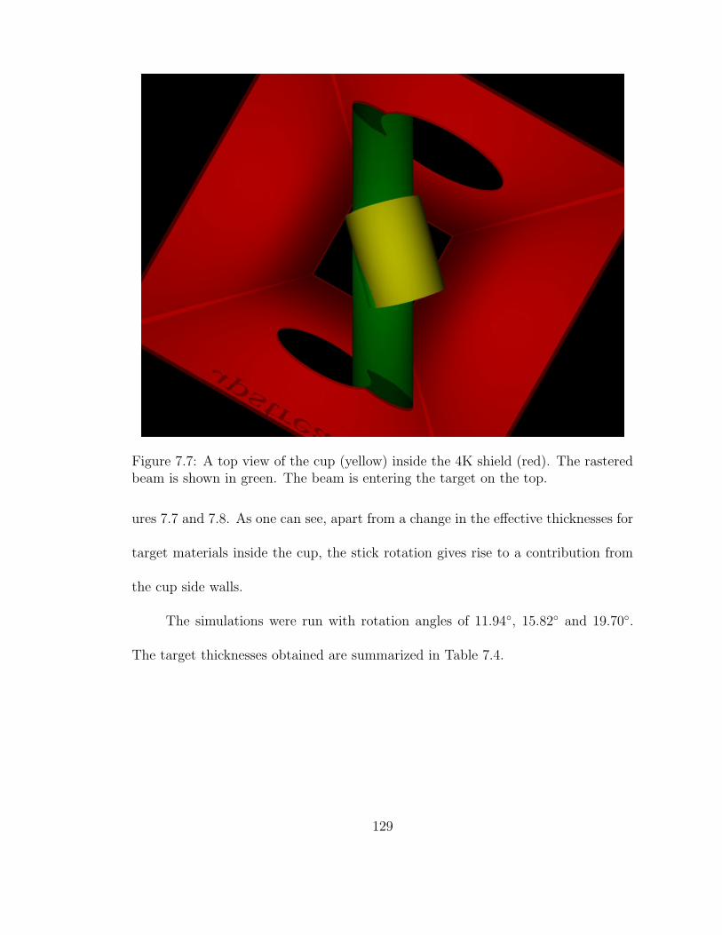
Figure 7.7: A top view of the cup (yellow) inside the 4K shield (red). The rasteredbeam is shown in green. The beam is entering the target on the top.
ures 7.7 and 7.8. As one can see, apart from a change in the effective thicknesses for
target materials inside the cup, the stick rotation gives rise to a contribution from
the cup side walls.
The simulations were run with rotation angles of 11.94, 15.82 and 19.70.
The target thicknesses obtained are summarized in Table 7.4.
129

Figure 7.8: Target insert rotation.
130
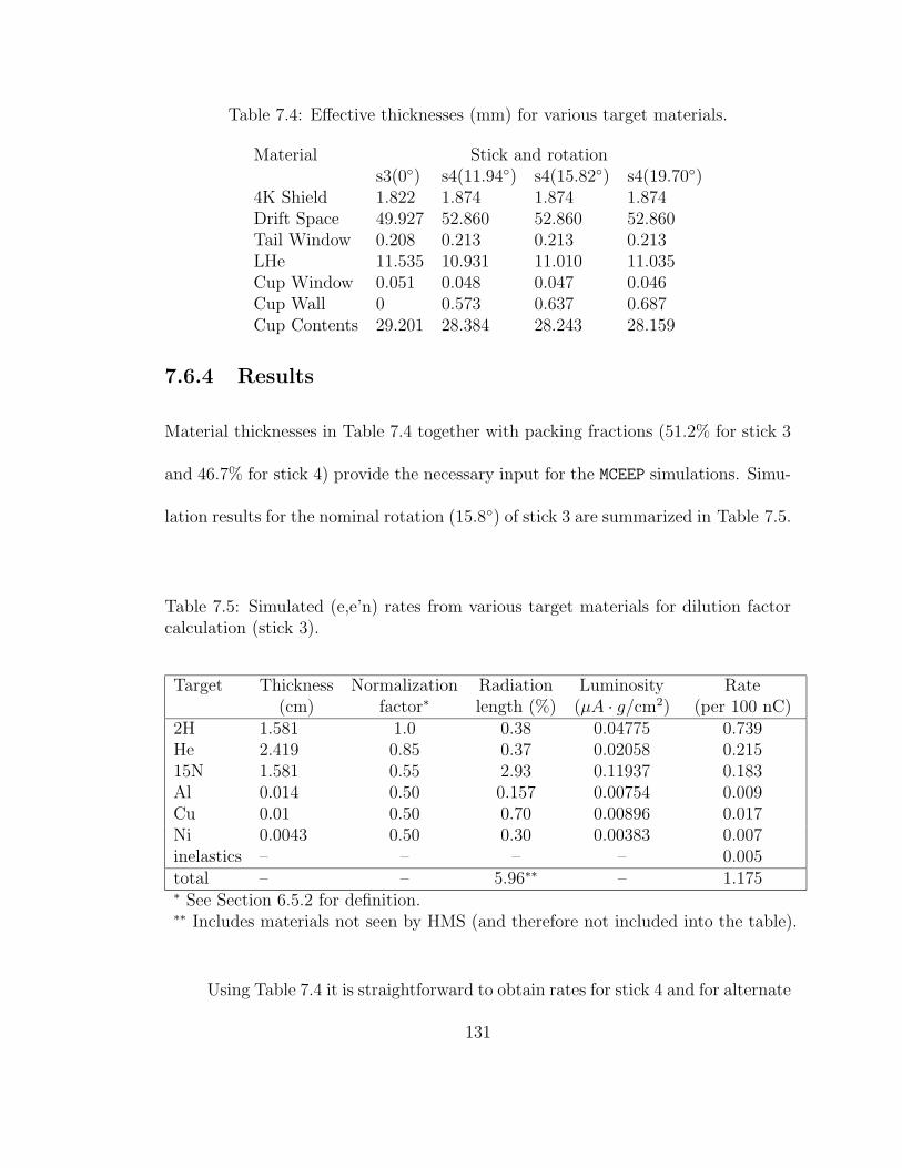
Table 7.4: Effective thicknesses (mm) for various target materials.
Material Stick and rotations3(0) s4(11.94) s4(15.82) s4(19.70)
4K Shield 1.822 1.874 1.874 1.874Drift Space 49.927 52.860 52.860 52.860Tail Window 0.208 0.213 0.213 0.213LHe 11.535 10.931 11.010 11.035Cup Window 0.051 0.048 0.047 0.046Cup Wall 0 0.573 0.637 0.687Cup Contents 29.201 28.384 28.243 28.159
7.6.4 Results
Material thicknesses in Table 7.4 together with packing fractions (51.2% for stick 3
and 46.7% for stick 4) provide the necessary input for the MCEEP simulations. Simu-
lation results for the nominal rotation (15.8) of stick 3 are summarized in Table 7.5.
Table 7.5: Simulated (e,e’n) rates from various target materials for dilution factorcalculation (stick 3).
Target Thickness Normalization Radiation Luminosity Rate(cm) factor∗ length (%) (µA · g/cm2) (per 100 nC)
2H 1.581 1.0 0.38 0.04775 0.739He 2.419 0.85 0.37 0.02058 0.21515N 1.581 0.55 2.93 0.11937 0.183Al 0.014 0.50 0.157 0.00754 0.009Cu 0.01 0.50 0.70 0.00896 0.017Ni 0.0043 0.50 0.30 0.00383 0.007inelastics – – – – 0.005total – – 5.96∗∗ – 1.175∗ See Section 6.5.2 for definition.∗∗ Includes materials not seen by HMS (and therefore not included into the table).
Using Table 7.4 it is straightforward to obtain rates for stick 4 and for alternate
131
rotations of stick 3. The dilution factor of the stick 3 is 62.7% for the nominal angle
and 62.8% for 11.94, i.e. the uncertainty in the rotation angle is about 0.1% relative.
For stick 4 the result is 62.6%. The uncertainty in the dilution factor was estimated
by comparing the measured rates with Monte Carlo predictions and was found to be
2.6% relative. With this, for the statistically weighted dilution factor for the entire
data set one has 62.6± 1.6%.
7.7 Corrections
Before the experimental asymmetry can be used for extraction of the GnE, it needs
to be corrected for dilution and/or contamination from unwanted background (ac-
cidental coincidences, multi-step reactions, misidentified protons), loss of events in
electronics (electronics deadtime) and bias of reaction kinematics due to electron
energy loss by radiation.
7.7.1 Radiative corrections
In the analysis of the experimental data we deal with measured values of the reaction
kinematics. These, however, in general may differ from the actual, or vertex kine-
matic quantities. The main mechanism responsible for this difference is radiative
energy loss by both incident and scattered electron.
Since the bremsstrahlung photons are not observed, one needs again to re-
sort to simulations to estimate the effect of these energy losses and correct for
132
it. The MCEEP imitates the effects of internal and external radiation by sampling
bremsstrahlung photons according to the bremsstrahlung spectrum. The photons
are emitted along the direction of either the incident or the outgoing electron (peak-
ing approximation). Radiative effects can be turned off by disabling the corre-
sponding option in the input file. The value of the acceptance averaged Monte
Carlo asymmetry with the radiation off is then compared with the nominal value
(radiation on) and the ratio between these two gives the desired radiative correction.
This procedure was done separately for internal and external radiative effects
and yielded a 0.55 ± 0.50% correction for the internal radiation. The correction
due to the external radiation was found small due to the statistical Monte Carlo
uncertainty of 0.50%
7.7.2 Paddle inefficiency
The particle identification algorithm was based on the hit in one of the paddle
planes. The probability for a proton to produce a hit in a paddle plane (i.e. paddle
efficiency) is very high, but still below 100%. A proton that did not fire a paddle
was likely to be identified as a neutron. As the protons have the asymmetry of
the opposite sign (compared to that of the neutrons) and have a larger quasielastic
scattering cross section, even a small paddle inefficiency can result in a sizeable
contamination of the neutron asymmetry.
The contribution of misidentified protons to the total measured neutron asym-
133

metry A can be found as:
A =N+
n −N−n +N+
p −N−p
Nn +Np
=
=NnAn +NpAp
Nn +Np
≈ An +Np
Nn
Ap, (7.6)
where N+(−)n(p) is neutron (proton) yield for positive (negative) beam helicity, An(p) is
the “clean” (uncontaminated) asymmetry of neutrons (protons), and we used the
fact that Np ¿ Nn.
Expressing the combined inefficiency of paddle planes ε through individual
plane efficiencies ε1,2 we obtain the following formula for the asymmetry contami-
nation ∆A:
∆A = (1− ε1)(1− ε2)Np
Nn
Ap. (7.7)
The paddle plane efficiencies were calculated using 2-out-of-3 (one paddle +
one bar) events in the first three detector planes and were found to be 96.0% and
98.3% for planes 1 and 2, correspondingly. The Np/Nn ratio was extracted from
our experimental data. It was found that initial proton-to-neutron ratio of 6:1 was
reduced by the θnq < 0.08 cut to 1:2. Finally, the proton asymmetry Ap was also
taken from our experimental data to be −15.2%. Plugging these numbers into the
Equation 7.7 we obtained the proton contamination correction of order 50 ppm,
i.e. about 1% of the size of the statistical error of the measured asymmetry, and
134
therefore negligible.
7.7.3 Electronics deadtime
When the counting rates in detectors are high, the data acquisition system may
start losing events. This is known as deadtime. The experimental deadtime can
be divided into computer deadtime (loss of events due to the BUSY status of the
DAQ) and electronics deadtime. The computer deadtime is taken care of by the
data stream preprocessor (see Section 6.2) and thus we only need to correct for the
electronics deadtime.
The loss of events in electronics occurs due to overlap of signals that have a
finite time width. Since the principal trigger in the experiment was the HMS trigger,
the neutron detector electronics did not contribute to the deadtime.
The HMS electronics generated HMS gates of 4 different widths: 30 ns, 60 ns,
90 ns and 120 ns. By observing the dependence of the event rate on the gate width
and extrapolating it to 0 ns one can find the “ideal” HMS rate. The deadtime is
then the difference between the 30 ns gate rate and this 0 ns extrapolated value.
Three randomly chosen runs were studied. Typical results are shown in Fig-
ure 7.9. The values of the correction is of the order of 15-30 ppm and thus is
negligible given the statistical accuracy of the experiment.
135
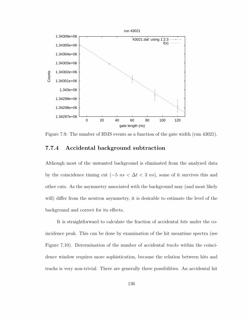
1.34297e+06
1.34298e+06
1.34299e+06
1.343e+06
1.34301e+06
1.34302e+06
1.34303e+06
1.34304e+06
1.34305e+06
1.34306e+06
0 20 40 60 80 100 120
Cou
nts
gate length (ns)
run 43021
’43021.dat’ using 1:2:3f(x)
Figure 7.9: The number of HMS events as a function of the gate width (run 43021).
7.7.4 Accidental background subtraction
Although most of the unwanted background is eliminated from the analyzed data
by the coincidence timing cut (−5 ns < ∆t < 3 ns), some of it survives this and
other cuts. As the asymmetry associated with the background may (and most likely
will) differ from the neutron asymmetry, it is desirable to estimate the level of the
background and correct for its effects.
It is straightforward to calculate the fraction of accidental hits under the co-
incidence peak. This can be done by examination of the hit meantime spectra (see
Figure 7.10). Determination of the number of accidental tracks within the coinci-
dence window requires more sophistication, because the relation between hits and
tracks is very non-trivial. There are generally three possibilities. An accidental hit
136
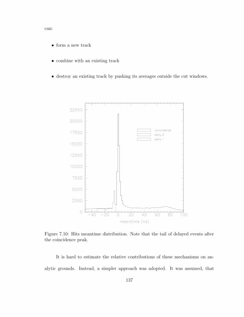
can:
• form a new track
• combine with an existing track
• destroy an existing track by pushing its averages outside the cut windows.
Figure 7.10: Hits meantime distribution. Note that the tail of delayed events afterthe coincidence peak.
It is hard to estimate the relative contributions of these mechanisms on an-
alytic grounds. Instead, a simpler approach was adopted. It was assumed, that
137

the relationship between the total number of tracks and the number of accidental
hits is approximately linear (for reasonably low background). Then the number of
“pure” tracks (no accidentals) can be obtained by extrapolating the dependence of
the track number on the level of background hits to zero background. The number
of background hits was controlled by adding extra coincidence windows.
Two such windows were used, “early 1” (−21.5 ns < ∆t < −11.0 ns) and
“early 2” (−32.0 ns < ∆t < −21.5 ns), both having the same width as the nominal
coincidence window (−3 ns < ∆t < 7.5 ns). The results are shown in Figure 7.11. A
straight line fit to the data points shows that our assumption of a linear relationship
between the number of background hits and the number of resulting tracks is valid.
The relative background (defined as the ratio of background to “clean” coinci-
dence tracks) is slightly different from the relative excess (ratio of background tracks
to all tracks) plotted in Figure 7.11. The relative background averages over the entire
sample of analyzed data (16 runs) are given in the Table 7.6. The global average was
calculated from background in windows early1, early2 and early12 using weighting
factors of 30%, 30% and 40% respectively, and was found to be 0.51± 0.23%.
Table 7.6: Background study results. ”Early12” refers to tracks with both early1and early2 windows open. The numbers are relative backgrounds (%), as defined inthe text.
counts early 1 early 2 early12 average error44583 0.62 0.43 0.49 0.51 0.23
138

-1
-0.5
0
0.5
1
1.5
2
2.5
0 1 2 3 4
rela
tive
trac
k ex
cess
(%
)
hit background level
datafit
Figure 7.11: Relative track excess (i.e. relative change in the number of tracks due toadditional background) versus the background level. The three points correspond tonormal data (coincidence window only), one extra “early” window, and both “early”windows.
7.7.5 Multi-step reactions contamination
The vast majority of neutrons detected in the neutron detector come from quasielas-
tic ~d(~e, e′n) scattering in the target material. However, a small fraction of neutron
events are brought up by charge exchange reactions in the lead curtain and the
target material. Additionally, decay of pions generated in the lead produces pho-
tons that cannot be distinguished from neutrons. Contributions from these reaction
mechanisms carry proton asymmetry, which has the opposite sign compared to the
neutron one, and therefore it is important to correct for these effects.
In the analysis of E93-026 the following multi-step reactions were investigated:
139

• in the lead shielding
– d(e, e′p) followed by 208Pb(p, n)
– d(e, e′p) followed by 208Pb(p, π0) and π0 → γγ
• in the target material
– d(e, e′p) followed by 15N(p, n)
Charge exchange in the deuteron itself is included in the theoretical calcula-
tions as a part of final state interactions and does not require a correction. Charge
exchange in other target materials does contribute to the scattering asymmetry, but
is negligible compared to the nitrogen.
Charge exchange in the lead
The size of the contribution of the charge exchange in the lead was estimated using
Monte Carlo simulations. For proton kinematics, actual distributions from experi-
mental data were used. The proton energy was corrected for the energy loss suffered
in the lead. The emitted neutron was generated using 208Pb(p, n) cross section from
the charge exchange studies of the Basel GnM experiment [73]. Since the angular
dependence of the 208Pb(p, n) cross section is not known, two extreme cases were
considered:
• same angular dependence as free p− n scattering
• no angular dependence
140
The straight average of the results for the two cases was used in the simulation.
The difference between the two answers (26.7%) was included in the systematic
uncertainty.
For simplicity, the neutron detector in the simulations was replaced with a
cube of dimensions given by the enclosure of all bar planes except the extended
top of plane 3. Neutron detection efficiency ε was calculated as a function of the
pathlength x, ε = exp(−αx). The constant α was calculated using the KSUVAX
program [71] and was found to be independent of neutron energy (within 10%) above
the threshold energy of 55 MeV.
As we noted earlier, the neutrons generated by charge exchange carry the pro-
ton asymmetry, therefore the simulation used actual proton asymmetries measured
in E93-026 as functions of various kinematic variables.
The resulting correction is −3.15% ± 3.01%. The error is dominated by the
uncertainty in the charge exchange cross-section [74].
7.8 Results
7.8.1 Extraction of GnE
The GnE extraction procedure is very straightforward. First, one calculates run by
run asymmetries (see Figure 7.13) and their statistically weighted average. Then
all relevant corrections are applied (accidental background, radiative effects, charge
141
exchange etc.). In parallel, one averages the theoretical asymmetry over the detector
acceptance for different values of GnE Finally, the Gn
E is found as the solution of
the equation Aexp = Atheor(GnE) (see Figure 7.12).
The time evolution of neutron asymmetries is shown in Figure 7.13(a). In
order to improve the statistical resolution, group averages (rather than run-by-run
asymmetries) are plotted there, where the groups are defined by changes in beam
and target polarizations. The scatter of individual points is purely statistical, as
confirmed by Figure 7.13(b) where a χ2 distribution for run-by-run asymmetries is
plotted in comparison with the theoretical curve.
The asymmetry was also calculated for proton events. Since proton form
factors are better known at our kinematics, proton asymmetries can be compared
to the theoretical predictions, thus providing a check of experimental systematics.
Also, we have much (roughly by a factor of six) more proton events thatn neutron
ones, and they carry a larger asymmetry, so the statistical resolution is much better
for protons. The results of the proton asymmetry study are shown in Figure 7.14.
The agreement between the theoretical calculations and experimentally measured
proton asymmetries is excellent.
The global average for the neutron asymmetry (corrected for beam and target
polarizations only) was found to be 4.031±0.471%. After applying the dilution factor
and other corrections it becomes 6.641±0.776%. The linear interpolation 7 between
the AVed values for Gn
E = 1.1 GGalster and GnE = 1.3 GGalster gives 0.0423 ± 0.00506
7Higher order effects are smaller than 0.05% (relative) and thus need not be considered.
142
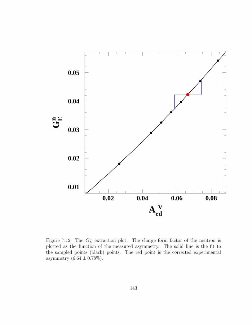
AedV
GEn
0.01
0.02
0.03
0.04
0.05
0.02 0.04 0.06 0.08
Figure 7.12: The GnE extraction plot. The charge form factor of the neutron is
plotted as the function of the measured asymmetry. The solid line is the fit tothe sampled points (black) points. The red point is the corrected experimentalasymmetry (6.64± 0.78%).
143
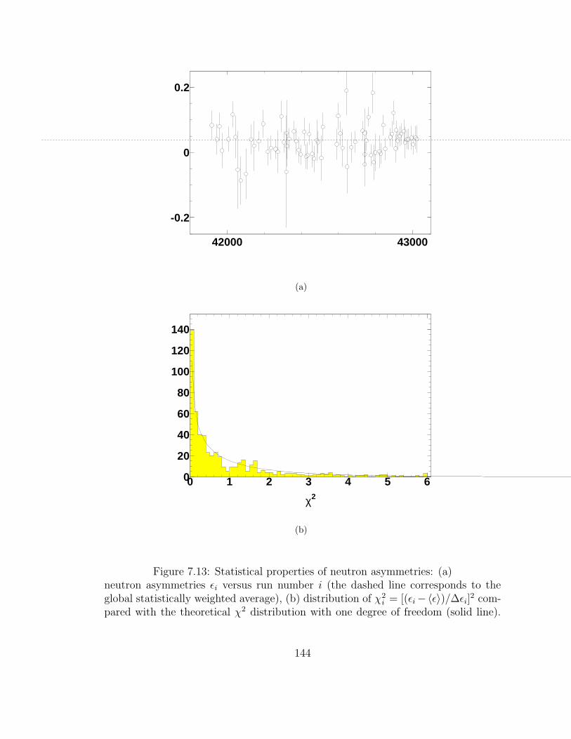
-0.2
0
0.2
42000 43000
(a)
0
20
40
60
80
100
120
140
0 1 2 3 4 5 6
χ2
(b)
Figure 7.13: Statistical properties of neutron asymmetries: (a)neutron asymmetries εi versus run number i (the dashed line corresponds to theglobal statistically weighted average), (b) distribution of χ2i = [(εi−〈ε〉)/∆εi]2 com-pared with the theoretical χ2 distribution with one degree of freedom (solid line).
144

-0.1
-0.05
0
850 900 950 1000
W (MeV)
-0.1
-0.05
0
2.8 2.9 3 3.1
E, (GeV)
-0.1
-0.05
0
-200 -100 0 100
Xpos (cm)
-0.1
-0.05
0
-40 -20 0 20 40
Ypos (cm)
Figure 7.14: Proton asymmetries: Monte Carlo (solid line) compared to data (opencircles).
for the GnE (1.172 GGalster ). When calculating the theoretical asymmetries, the
dipole parametrization for the magnetic form factor of the neutron was assumed.
However, recent measurement indicate that the true value of GnM deviates from the
dipole parametrization: GnM/GD = 1.072±0.014 [75]. Monte Carlo simulations with
different values of GnM showed that its effect on the Gn
E is linear. With this, the
final value for the GnE becomes:
GnE = 0.0454± 0.0054, (7.8)
where the uncertainty is statistical. Systematic uncertainties will be considered in
the remainder of the section.
145
7.8.2 Kinematic uncertainties
The leading kinematic uncertainty is due to the horizontal position of the neutron
detector. The initial comparison between ypos (i.e. horizontal position of the nucleon
track at the 3rd plane) spectra of the data and the Monte Carlo revealed a 4 cm
discrepancy which was attributed to a bias in the survey measurement of the neutron
detector angle. In order to determine the impact of this uncertainty, the data
analysis was repeated with a shifted neutron detector position.
This showed that a 5 mrad shift in the neutron detector angle changes the AVed
(and therefore, GnE ) by 2.4%. Since a 4 cm shift in ypos corresponds to a 6.4 mrad
shift in the angle, the uncertainty due to the neutron detector position is 3.22%.
The next largest kinematic uncertainty is the one due to the field angle. This
quantity was measured by surveyors to the accuracy of 0.1, which propagates to
0.99% uncertainty in AVed, as found by Monte Carlo simulation with a shifted target
field orientation. Other kinematic uncertainties were also studied using Monte Carlo
simulations and were found to have a small impact (see Table 7.7).
7.8.3 Other experimental uncertainties
The combined kinematic uncertainty together with other sources of the systematic
error are given the Table 7.8. The largest uncertainty is the one related to the target
polarization (4.6%). Other important contributions include the combined kinematic
uncertainty, beam polarization error and the charge exchange uncertainty.
146
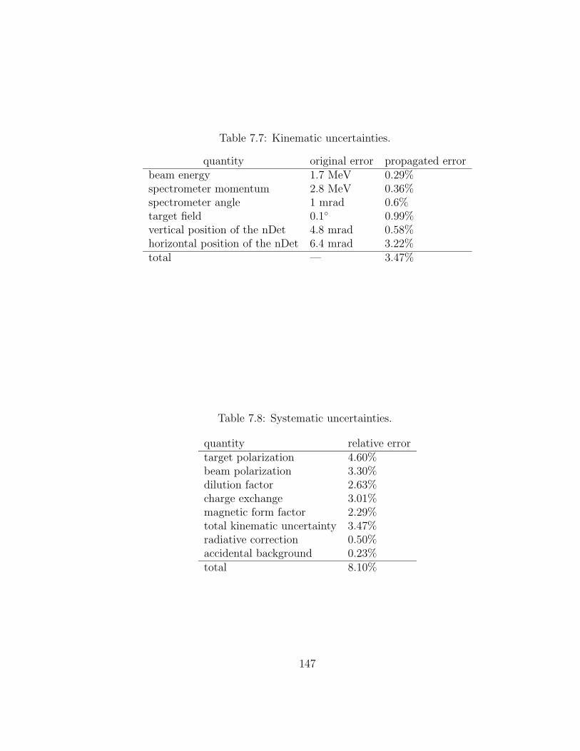
Table 7.7: Kinematic uncertainties.
quantity original error propagated errorbeam energy 1.7 MeV 0.29%spectrometer momentum 2.8 MeV 0.36%spectrometer angle 1 mrad 0.6%target field 0.1 0.99%vertical position of the nDet 4.8 mrad 0.58%horizontal position of the nDet 6.4 mrad 3.22%total — 3.47%
Table 7.8: Systematic uncertainties.
quantity relative errortarget polarization 4.60%beam polarization 3.30%dilution factor 2.63%charge exchange 3.01%magnetic form factor 2.29%total kinematic uncertainty 3.47%radiative correction 0.50%accidental background 0.23%total 8.10%
147

Since the asymmetry depends not only on the charge form factor of the neu-
tron, but also on the magnetic one, which is known with a limited accuracy, the
GnM uncertainty of 2.29% must also be included. The overall error is obtained by
combining all partial errors in quadrature and is found to be 8.10%. With this, the
final result of the experiment becomes:
GnE(Q
2 = 1.0) = 0.0454± 0.0054(stat)± 0.0037(sys). (7.9)
7.8.4 Reaction mechanism dependence
In order to investigate the effects of various aspects of the reaction mechanism on the
extracted value of GnE the extraction procedure was repeated with the values of the
theoretical asymmetries calculated in two simplified models: PWIA+RC (relativis-
tic impulse approximation) and FSI+RC (the former plus final state interactions).
Since we are only interested in the relative size of various nuclear corrections and
since the relation between the extracted GnE and the model value of Gn
M is linear,
the dipole parametrization was used for GnM for all three models.
The results of this study are presented in Table 7.9. The effects of the meson
exchange currents and isobar configurations are thus small (of order of 2%), whereas
the effect of the final state interactions is somewhat bigger (∼ 5%).
These numbers compare very favorably to analogous estimates for the un-
polarized measurements, where the effects of nuclear corrections of 10 − 30% are
148

typical. Also, comparison with calculations for Q2 = 0.5 (10.5% difference from the
full calculation for PWBA+RC and 2.4% for FSI+RC) show that these corrections
become relatively less important at higher Q2.
The impact of the choice of the N − N potential on the AVed is negligible for
quasifree kinematics [36].
Table 7.9: Reaction mechanism dependence of GnE All calculations assume dipole
parametrization for GnM .model Gn
E impact(%)Full 0.0423 –PWBA + RC 0.0397 6.1FSI + RC 0.0415 1.9
7.8.5 Parametrization of GnE
Traditionally, GnE is parametrized using the so-called Galster parametrization
GGalster = −aµnτ
1 + bτGD, (7.10)
with a = 1, b = 5.6, GD = (1+Q2/Λ2)−2 and Λ = 0.71 (GeV/c)2. This parametriza-
tion, based on low-Q2 data from early 1970’s [16], continues to work well even for
higher Q2 data. However, the improved precision data from this experiment and the
results of a recent recoil polarimetry measurement in JLab Hall C [27] now reveal a
sizeable deviation from the conventional Galster fit.
We performed a fit to the world GnE database using the traditional Galster
form (7.10). The fitting procedure yielded a = 0.86 ± 0.04 and b = 3.06 ± 0.46
149

with the χ2 per degree of freedom of 0.71. The charge radius measurement [10]
was included into the fitted database to constrain the slope of GnE at low Q2. The
comparison of the fit with the experimental data can be seen in Figure 7.15.
0
0.05
0.1
0 0.2 0.4 0.6 0.8 1 1.2 1.4 1.6 1.8 2
Q2 [ GeV2 ]
GE
n
Figure 7.15: Results of the 2001 run of E93-026 (2001 run – red stars, 1998 run –cyan triangle) compared with other experimental data (see Figure 8.7 for descriptionof the markers). The solid line is the improved Galster fit of Section 7.8.5.
150
Chapter 8
Theoretical predictions of GnE
8.1 Asymptotic behavior
Modern physics sees the nucleon as three valence quarks dressed with a sea of quark-
antiquark pairs, interacting by means of gluon exchange. The ultimate description
of the nucleon is to be given by quantum chromodynamics (QCD). At the low and
intermediate momentum transfers the QCD calculations are not feasible (due to ex-
treme nonlinearity of the interaction). At the high momentum transfers, however,
the quarks behave as free particles (this feature of QCD is known as asymptotic
freedom). Therefore, for large Q2 the running coupling constant of the strong inter-
action αs(Q2) becomes small and perturbative techniques can be applied.
8.1.1 Dimensional scaling laws
Certain conclusions about the asymptotic behavior of the form factors can be made
without performing the actual perturbative QCD (pQCD) calculations. Consider
151
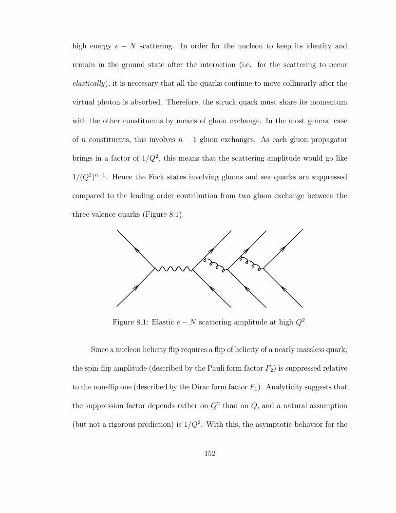
high energy e − N scattering. In order for the nucleon to keep its identity and
remain in the ground state after the interaction (i.e. for the scattering to occur
elastically), it is necessary that all the quarks continue to move collinearly after the
virtual photon is absorbed. Therefore, the struck quark must share its momentum
with the other constituents by means of gluon exchange. In the most general case
of n constituents, this involves n − 1 gluon exchanges. As each gluon propagator
brings in a factor of 1/Q2, this means that the scattering amplitude would go like
1/(Q2)n−1. Hence the Fock states involving gluons and sea quarks are suppressed
compared to the leading order contribution from two gluon exchange between the
three valence quarks (Figure 8.1).
Figure 8.1: Elastic e−N scattering amplitude at high Q2.
Since a nucleon helicity flip requires a flip of helicity of a nearly massless quark,
the spin-flip amplitude (described by the Pauli form factor F2) is suppressed relative
to the non-flip one (described by the Dirac form factor F1). Analyticity suggests that
the suppression factor depends rather on Q2 than on Q, and a natural assumption
(but not a rigorous prediction) is 1/Q2. With this, the asymptotic behavior for the
152
Dirac and Pauli form factors becomes [76]
F1 ∼ 1/Q4, (8.1)
F2 ∼ F1/Q2. (8.2)
The equations 8.1 and 8.2 are known as dimensional scaling laws.
If one expresses F1 and F2 in terms of Sachs form factors, one arrives at the
1/Q4 asymptotic dependence for both GE and GM .
8.1.2 Perturbative QCD calculations.
Magnetic form factors
The dimensional scaling laws only give the leading power asymptotic behavior for
Q2 → ∞. More information (normalizations, logarithmic corrections, etc.) can be
obtained by performing the actual pQCD calculations.
The perturbative approach is based on QCD factorization theorems, which
allow scale separation between the short-distance and long-distance motion of the
partons. The short-distance (high momentum) motion corresponds to hard (per-
turbative) physics, while long-distance (low momentum) motion corresponds to soft
(non-perturbative) physics.
153

For the helicity conserving form factor of the nucleon1 one has in pQCD :
F1(Q2) =
∫ 1
0
[dxi]
∫ 1
0
[dyi]φ†(xi, Q)TH(xi, yi, Q)φ(yi, Q), (8.3)
where TH(xi, yi, Q) is the hard scattering amplitude, φ(xi, Q) is the minimum Fock-
state wave function integrated over transverse momenta, xi is the longitudinal mo-
mentum fraction carried by the i-th valence quark, and [dxi] = dx1dx2dx3δ(1−∑
i xi).
It is straightforward to express TH in terms of momentum fractions xi. The situa-
tion is more complicated with the soft wavefunction φ(yi, Q). By using QCD sum
rules, one can extract the moments of this wavefunction from the experimental data.
Since only a finite number of moments is known, such parameterizations are model-
dependent. If one is only interested in the logarithmic corrections, one can use an
expansion of φ(xi, Q) in a series of eigensolutions of the evolution equation [77].
φ(xi, Q) = x1x2x3
∞∑
n=0
anφn(xi)
(
lnQ2
Λ2
)−γn
, (8.4)
where Λ is the QCD scale parameter, and an and γn are some constants. Calculations
performed with the soft wavefunction (8.4) give for the form factor F1:
F1(Q2) =
32π2
9
α2s(Q2)
Q4
∑
n,m
bn,m
(
lnQ2
Λ2
)−γn−γm
[1 +O(αs(Q2),m/Q)]. (8.5)
Since the helicity-flip amplitude (associated with the Pauli form factor F2) is sup-
1Or more generally, any baryon.
154

pressed for high Q2, for the leading term of the left-hand side of the Equation 8.5
can be replaced with GM :
GM(Q2)→ 32π2
9C2
α2s(Q2)
Q4
(
lnQ2
Λ2
)−4/3β(e|| − e−||), (8.6)
where e|| (e−||) is the mean charge of quarks with helicity parallel (antiparallel)
to the baryon’s helicity (for nucleons ep|| = 1, ep−|| = 0, en|| = −13and en−|| =
13),
β = 11− (2/3)nflavor.
Electric form factors
The contribution of the Pauli form factor F2 to the electric form factor GE is am-
plified by a factor of Q2 and therefore cannot be neglected in the limit of Q2 →∞.
As we have already mentioned earlier, F2 is related to the helicity-flip amplitude.
There are two mechanisms of a hadron helicity flip: quark masses and quark orbital
angular momentum. Since the quark masses are small, it is generally believed that
the latter mechanism is dominant.
Therefore, calculating the Pauli form factor F2 requires augmentation of the
standard formalism with the parton orbital momentum. This technology has been
recently developed by Burkardt, Ji and Yuan [78]. Based on it, Belitsky, Ji and
Yuan have performed the calculations [79]. By using so called collinear expansion
(expansion of the hard part of the diagram in k2i /Q2, where ki are quark transverse
155

Figure 8.2: A two-gluon exchange hard scattering diagram for F p2 . Permutations
and mirror images need to be added.
momenta), they express F p2 in terms of twist-3 and 4 amplitudes Φ3, Φ4 and Ψ4 as
F p2 (Q
2) =
∫
[dx][dy] x3Φ4(x1, x2, x3)TΦ(x, y)
+x1Ψ4(x2, x1, x3)TΨ(x, y)Φ3(y1, y2, y3) , (8.7)
where x = (x1, x2, x3), the square brackets have the same meaning as in (8.3), and
TΨ,Φ are hard scattering diagrams (Figure 8.2 and its permutations and reflections).
The exact solutions for the wavefunctions Φ3, Φ4 and Ψ4 can only be obtained by
solving QCD non-perturbatively. However, their asymptotic form for large Q2 is
known [80]:
Φ3 ∼ x1x2x3,Φ4 ∼ x1x2,Ψ4 ∼ x1x3. (8.8)
When trying to calculate (8.7) with wavefunctions (8.8) one ends up with diver-
156

gent (due to end-point singularities) integrals. The authors argue that higher-order
pQCD resummation (the Sudakov form factor) provides an effective cut-off for the
integrals at small x ∼ Λ2/Q2, where Λ is a soft scale parameter related to the size
of the nucleon. As a result, the Pauli form factor receives an additional logarith-
mic correction compared to the Dirac form factor, and the high-Q2 prediction (8.2)
modifies to:
Q2F2(Q2)/F1(Q
2) ∼ ln2+8/(9β)Q2/Λ2. (8.9)
where for practical purposes the 8/(9β) term can be neglected.
8.1.3 Comparison with experiment
At the moment, accurate high-Q2 data is available only for GpM . Gn
M and GpE have
only been measured at moderate Q2 (up to 4 and 6 (GeV/c)2 correspondingly),
while GnE is yet to be explored at Q2 > 1.5 (GeV/c)2.
The Figure 8.3 shows the magnetic form factor of the proton (for convenience
plotted as Q4GpM). The asymptotic behavior appears to set in at approximately
5 (GeV/c)2 (the slow variations observable at high Q2 can be ascribed to log cor-
rections).
Whether or not this means that pQCD is valid at the Q2 of a few (GeV/c)2,
is still an open question. Skeptics believe that the agreement between the GpM
behavior and the pQCD predictions is mere luck. It has even been claimed that no
reasonable wavefunction can reproduce the correct normalization of the form factors
157
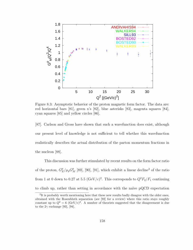
0
0.2
0.4
0.6
0.8
1
1.2
1.4
1.6
1.8
5 10 15 20 25 30
Gp M
(Q2 )Q
4
Q2 [(GeV/c)2]
ANDIVAHIS94WALKER94
SILL93BOSTED92BOSTED90WALKER89
Figure 8.3: Asymptotic behavior of the proton magnetic form factor. The data are:red horizontal bars [81], green x’s [82], blue asterisks [83], magenta squares [84],cyan squares [85] and yellow circles [86].
[87]. Carlson and Gross have shown that such a wavefunction does exist, although
our present level of knowledge is not sufficient to tell whether this wavefunction
realistically describes the actual distribution of the parton momentum fractions in
the nucleon [88].
This discussion was further stimulated by recent results on the form factor ratio
of the proton, GpE/µpG
pM [89], [90], [91], which exhibit a linear decline2 of the ratio
from 1 at 0 down to 0.27 at 5.5 (GeV/c)2. This corresponds to Q2F2/F1 continuing
to climb up, rather than setting in accordance with the naıve pQCD expectation
2It is probably worth mentioning here that these new results badly disagree with the older ones,obtained with the Rosenbluth separation (see [92] for a review) where this ratio stays roughlyconstant up to Q2 = 6 (GeV/c)2. A number of theorists suggested that the disagreement is dueto the 2γ exchange [93], [94].
158
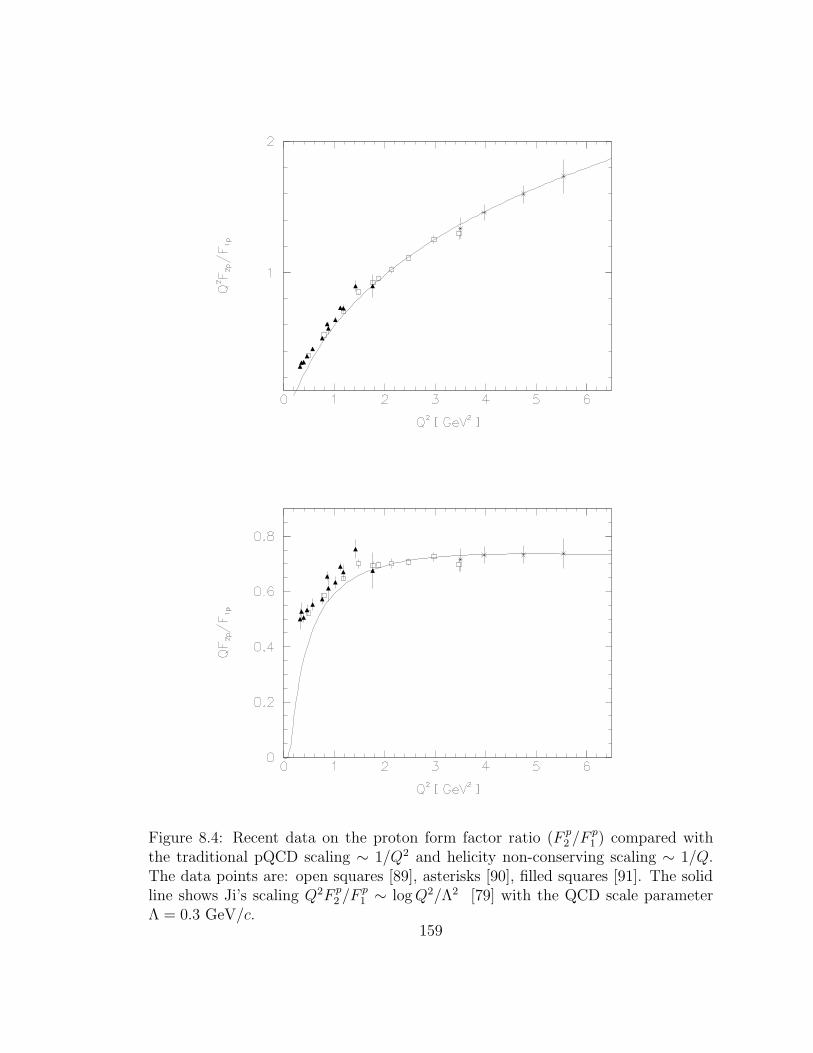
Figure 8.4: Recent data on the proton form factor ratio (F p2 /F
p1 ) compared with
the traditional pQCD scaling ∼ 1/Q2 and helicity non-conserving scaling ∼ 1/Q.The data points are: open squares [89], asterisks [90], filled squares [91]. The solidline shows Ji’s scaling Q2F p
2 /Fp1 ∼ logQ2/Λ2 [79] with the QCD scale parameter
Λ = 0.3 GeV/c.159
Q2F2/F1 ∼ 1 (see Figure 8.4). One possible explanation is that the truly asymptotic
regime does not occur until much higher Q2 (of at least 10 (GeV/c)2), and the early
scaling of GpM is accidental.
As an alternative explanation, some theorists have pointed to the violation
of hadron helicity conservation (HHC) rule [95]. The HHC rule is a natural conse-
quence of the pQCD factorization scheme. The hard scattering kernel is azimuthally
symmetric to the leading order. The dependence on the azimuthal angle comes from
the quark transverse momenta, k± = (kx ± iky) = |~k⊥| exp(±iφ), which are small
compared to the large momentum transfer, |~k⊥| ∼ ΛQCD ¿ Q [96]. If the quark
orbital angular momentum in the initial and the final states differs by ∆m units, the
integrand in the pQCD factorization integral will receive a factor of exp(i∆mφ). In
order to survive the integration by dφ this factor needs to be cancelled by a corre-
sponding term from the expansion of the hard kernel in the transverse momentum.
As a result, the contribution from the quark orbital angular momentum (OAM)
becomes suppressed by (k±⊥/Q)∆m ∼ (ΛQCD/Q)∆m. Since quark current masses are
small and cannot flip the hadron helicity, suppression of the contribution from the
quark OAM leads to the conservation of the helicity of the hadron, i.e. the HHC
rule.
Critics of the HHC stress that despite the theoretical attraction of the HHC
rule, there are many experimental situations in which helicity conservation is not
observed [97]. Further, it is argued that by making some simple assumptions (which
160
are not in conflict with the pQCD itself, but rather with the specific “asymptotic
short distance” approach used in HHC derivation) one arrives at the scaling law of
QF2/F1 ∼ const, (8.10)
which fits the observed data quite well [95], [98].
However, the result of the direct pQCD calculation by Belitsky, Ji and Yuan
described in the previous section, is also in an excellent agreement with the JLab
data. Thus, the behavior of the F2/F1 ratio for the proton can be interpreted as
a consequence of the QCD logarithmic corrections (as earlier suggested by Brod-
sky [77]) rather than an evidence in favor of the HHC violation. It should be noted
though, that the authors do not insist that the observed scaling of the JLab data
with (8.9) is a truly asymptotic behavior. They remark that their calculation of
Q6F p2 (Q
2) with asymptotic wavefunctions of [99] recovers only 1/3 of the JLab ex-
perimental value at Q2 = 5 (GeV/c)2. From that they conclude that higher-order
corrections and higher-twist effects are still important at this kinematics, and sug-
gest that the scaling may be a precocious one which owes its existence to some subtle
cancellations in the ratio.
161
8.2 Dispersion relations
In the theory of functions of a complex variable, the analyticity of a function re-
quires its real and imaginary parts to be related to each other by means of so called
dispersion relations (DR). If one defines the four momentum transfer on the complex
plane and imposes some constraints due to the properties of the scattering matrix
and the analytic behavior of the scattering amplitudes (so called unitarity and su-
perconvergence requirements), then one arrives to a set of integral equations relating
elastic form factors F1,2 to the absorptive ones F1,2 [4]:
F1,2(Q2) = F1,2(0)−
Q2
π
∫ ∞
4m2π
dzF1,2(z)
z(z +Q2 − iε) . (8.11)
The relations (8.11) are also known as spectral mass representations, and the
absorptive form factors are called spectral functions. The spectral functions charac-
terize the nucleon structure as probed by a timelike (i.e. Q2 < 0) virtual photon and
contain contributions from all states coupled to the NN state that can be produced
electromagnetically. Thus it is difficult to calculate the right-hand side (8.11) on
purely analytical grounds. Therefore, in order to use the dispersion relations formal-
ism for calculation of the elastic form factors, one needs to make further assumptions
about the form of the spectral functions.
The simplest way to address the dispersion relations (8.11) is by assuming
complete dominance of its right-hand side by low-lying resonances. This approach
162
(known as vector meson dominance) will be discussed in the next subsection.
A recent DR analysis of the elastic form factors of the nucleon by Mergell et
al. [100] employs a more sophisticated model, which uses the extended unitarity
relation of Frazer and Fulco [101] to express the absorptive isovector form factors in
terms of the πN P-wave partial wave amplitude and the pion form factor corrected
for ρ−ω mixing. In addition to the two-pion contribution, three heavier excitations
ρ′, ρ′′ and ρ′′′ were added to the model and were found to have a significant impact.
The low-Q2 behavior of the form factor was fixed by the experimental data on
nucleon charge radii, whereas the asymptotic behavior at high-Q2 was determined
by built-in constraints from the perturbative QCD.
8.3 Vector Meson Dominance
The concept of the vector meson dominance (VMD) was introduced by Sakurai [102].
The basic idea is that the interaction of a (virtual) photon with a nucleon is dom-
inated by quark-antiquark pairs which overlap with vector meson states. In the
language of dispersion relations this means that the mass spectral functions can
be well approximated by a set of delta functions corresponding to sharp meson
resonances:
FV,S1 (Q2) =
∑
i
Aiδ(Q2 +m2
i ), (8.12)
163
where the superscripts V, S refer to isovector (V) and isoscalar (S) form factors,
i = ρ, ω, φ... is the mesonic index, mi is the mass of the meson, and Ai are constants
depending on photon-meson and meson-nucleon coupling strengths. It is straight-
forward to see from Equation 8.11 that each delta function will result in a pole-like
term
Ai/(1 +Q2/m2). (8.13)
The pole-like form factors of VMD were very successful in describing the early (low
Q2) form factor data. In fact, the prediction of existence of the ρ meson by Nambu
in 1957 was inspired by the experimental results on the proton and neutron form
factors [103]. However, the asymptotic behavior of the monopole form factors (8.13)
is at odds with the dimensional scaling laws (8.1) and (8.2). Therefore, modern VMD
models are forced to have a correct asymptotic behavior by either using “intrinsic”
form factors or adding phenomenological terms.
The first work to include the pQCD asymptotics into a VMD model was that
of Gari and Krumpelmann [104]. They used the extended version of VMD (EVMD)
where the photon-nucleon interaction has a purely photonic part in additional to
the traditional meson poles. A complete decoupling of the φ meson from the nu-
cleon with accordance to the OZI rule3 [105] was assumed. Thus, the isovector and
3The OZI (Okubo-Zweig Iizuka) rule states that the disconnected (“hairpin”) diagrams are sup-pressed with respect to the continuous quark line graphs. According to this rule, non-strangenessof the nucleon means that coupling with the strange mesons (φ, K) is small [105], [106], [107],[108].
164

isoscalar form factors were determined by the ρ and ω mesons correspondingly:
F IV1 (Q2) =
[
m2ρ
m2ρ +Q2
gρfρ
+
(
1− gρfρ
)]
F1(Q2) (8.14)
κV FIV2 (Q2) =
[
m2ρ
m2ρ +Q2
κρgρfρ
+
(
κV −κρgρfρ
)]
F2(Q2) (8.15)
F IS1 (Q2) =
[
m2ω
m2ω +Q2
gωfω
+
(
1− gωfω
)]
F1(Q2) (8.16)
κV FIS2 (Q2) =
[
m2ω
m2ω +Q2
κωgωfω
+
(
κS −κωgωfω
)]
F2(Q2). (8.17)
The intrinsic Dirac and Pauli form factors were taken in a form providing the pQCD
high-Q2 behavior:
F1(Q2) =
Λ21
Λ21 + Q2Λ22
Λ22 + Q2(8.18)
F2(Q2) =
Λ21
Λ21 + Q2
[
Λ22
Λ22 + Q2
]2
, (8.19)
where Q2 = Q2 log(
Λ22+Q2
Λ2QCD
)
/ log(
Λ22Λ2QCD
)
. A simultaneous fit to available at that
moment cross-section data yielded an excellent χ2 per degree of freedom of 0.43 and
the values of free fit parameters were found to be close to the SU(3) expectations
(or experimental values).
In a later work [109] Gari and Krumpelmann upgraded their model to include
the effects of the strangeness content of the nucleon and introduced a helicity-flip
scale. By that time (1992), more experimental data on the nucleon form factors
have become available, including SLAC measurements of the GpE/G
pM ratio with
the Rosenbluth method. It was demonstrated that the increase of the GpE over the
165
dipole value GD could be achieved by setting the helicity-flip scale to the meson
scale, whereas the traditional model with the helicity-flip scale equal to the QCD
scale ΛQCD results in a decline of GpE with respect to the GD. Another interesting
result of this work is that the GnE is sensitive to the contribution from the φ meson
at moderate Q2, and therefore can serve as a probe of the strange content of the
neutron.
The work in this direction was continued by Lomon [110]. He studied two
families of models: three models based on the original Gari-Krumpelmann approach
(“GK models”) and four models with the ρ-meson pole replaced by a ρ′(1450)-meson
pole plus an approximation for the ρ-meson term in the dispersion-relations integral
from [100] (“DR-GK” models). The members of a model family differ between
themselves only by details of cut-off and normalization parameters. It was found
that the GK-DR model generally give a better agreement with the data than the
GK fits. The relatively high χ2 of the fits (about twice the number of degrees of
freedom) was explained by inconsistencies between different experimental data sets.
8.4 Quark models
8.4.1 Nonrelativistic quark models
The picture of a nucleon4 as consisting of three quarks in a confining potential
started to emerge in early 1960-s in pioneering works of Zweig [106], Gell-Mann [111]
4More generally, any baryon.
166
and many others. Despite its simplicity, the model had remarkable successes in
explaining hadronic mass spectra and radiative transition amplitudes, and is still
widely used nowadays.
The key element of the model is the SU(6) spin-flavor symmetry5 which allows
to make two important predictions about the form factors without even making
any specific assumptions about the quark-quark interaction potential. Namely, the
ratios of the form factors for finite Q2 remain same as for the static case (Q2 = 0),
i.e. GnM/G
pM = −2/3, Gn
E/GpE = 0 [112].
One example of a non-relativistic quark model is the model of Isgur, Karl and
Sprung [113] built on the analogy between QCD and QED. The confining poten-
tial is just the harmonic oscillator potential. The potential responsible for lifting
the degeneracy of the mass multiplets of hadrons is analogous to magnetic-dipole-
magnetic-dipole interactions of electromagnetism. Their results for the proton and
neutron charge form factors
GnE(Q
2) =1
6〈r2〉nQ2e−Q2/6α2 , (8.20)
GpE(Q
2) = e−Q2/6α2 . (8.21)
are in a qualitative agreement with the experiment for low Q2. However, the model
is only valid for Q up to the constituent quark mass (i.e. a few hundred MeV/c2).
5This symmetry is only approximate (unlike e.g. exact SU(3) color symmetry).
167
8.4.2 Relativistic constituent quark models
The naıve picture of the nucleon sketched in the previous section is obviously an
oversimplification. In reality the u and d quarks are about two orders of magnitude
lighter than the hadrons they make up, and in addition to the three valence quarks
there are gluons and quark-antiquark pairs (sea quarks). The success of the simple
quark model suggests that sea and glue degrees of freedom are frozen, while their
effects are hidden in the constituent (as opposed to physical, or current quarks)
quark masses. However, one problem still remains: quark momenta are much higher
than their masses, i.e. the quarks are highly relativistic. There have been a number
of attempts to add relativity to the constituent quark model.
In the relativistic case there exists three distinct forms of the Hamiltonian
dynamics, differing by what generators of the Poincare group6 are kinematical (i.e.
interaction-free): instant form, point form and light-cone form [114]. In the point
form (PF) and light-cone (LC) representations boosts are kinematic, and therefore
they are particularly suitable for studying the form factors (it is easy to transform
results obtained in one frame into any other frame).
Light-cone
The light-cone dynamics is formulated in so-called light front variables, x1, x2, x−
and x+, rather than ordinary world-point coordinates x1, x2, x3 and x4. As was first
6Poincare group is also known as the inhomogeneous Lorentz group. It is an extension of thetraditional Lorentz group of Lorentz boosts and spatial rotations by space-time translations.
168

demonstrated by Berestetskiy and Terentiev [115], this substitution leads to signif-
icant simplifications in form factor calculations. Consider the relativistic energy-
momentum relation:
pµpµ +m2 = 0. (8.22)
In terms of the light-cone variables p+, p− and ~p⊥ = (p1, p2) this becomes:
2p+p− − (p⊥)2 +m2 = 0. (8.23)
On the LC, the plus component of the momentum has the meaning of the Hamil-
tonian, H = −p+. If we introduce notation µ = p− we put Equation 8.23 into a
familiar form:
H = (p2⊥ +m2)/2µ, (8.24)
which is nothing else than the nonrelativistic Schrodinger equation for a particle
of mass µ on a two-dimensional plane. This analogy with the non-relativistic case
is very helpful, since it implies impossibility of creating virtual pairs with finite
energies due to conservation of µ = p− [115].
Chung and Coester [116], inspired by these advantages, performed an ex-
ploratory computation of nucleonic form factors using exactly Poincare-covariant
wavefunction, Gaussian in the quark momenta, from [117]:
φ(M0) =N(mq/ΛQCD)
Λ2QCD
exp(−M 20 /2Λ
2QCD), (8.25)
169

where M 20 =
(
∑
i
√
m2i + ~q2i
)2
,mi = mq are quark masses (assumed to be equal),
qi are the quark relative momenta, N is the normalization factor and ΛQCD is the
familiar confinement scale. They found that the data can be satisfactorily described
by the model if one uses small quark masses (0.24 GeV as opposed to the traditional
value of 0.33 GeV) and a somewhat large QCD scale parameter (0.635 GeV). The
quark form factors did not have any Q2 dependence.
The most recent studies within the framework of the light-cone dynamics were
carried out by Cardarelli and Simula [1], [118], [119]. In [118] the authors consider
Isgur’s cancellation mechanism and confirm the result of [11] to show that GnE can
indeed be interpreted as a measure of the charge distribution in the neutron. They
establish that retaining the leading order in the relativistic expansion of [11] corre-
sponds to neglecting the transverse motion of quarks in the Melosh rotations of the
initial state, and show that in this approximation (which they call the zitterbewe-
gung approximation) the non-relativistic SU(6) result GnE = 0 still holds. Further,
they use an example of a harmonic oscillator wavefunction of [113] to show that
full Melosh rotations break SU(6) symmetry and generate non-zero GnE on a level
that qualitatively explains the existing experimental data (although only 40% of the
neutron charge radius could be reproduced).
In [1] Cardarelli and Simula further improved their model by including dynam-
ical SU(6) symmetry breaking via spin-dependent quark-quark interactions and by
using the y-component of the electromagnetic current (rather than the plus compo-
170
nent)7 for the magnetic form factors. They show that although both non-relativistic
and zitterbewegung approximations fail to describe the experimental data even with
the dynamic SU(6)-breaking effects included, full light-cone calculations with the
wavefunction of the one-gluon exchange model [120] agree with the experimen-
tal data on the EMFFN (including the JLab results on GpE/G
pM [91]) fairly well.
However, the neutron charge form factor is still underestimated (only 65% of the
experimental value was reproduced).
A better agreement with the experiment can be achieved by using constituent
quark form factors, as done by Simula in [119]. There he uses the low-Q2 experimen-
tal data (up to 1 GeV/c) to fix the parameters of the constituent quark form factors,
so the higher Q2 predictions can be considered to be in a sense parameter-free.
Point-form
In the point-form representation all interaction is contained in the four-momentum
operators, which commute among themselves and thus can be simultaneously diag-
onalized. As with the light-cone dynamics, boost operators are interaction-free.
The point-form dynamics formalism was recently applied to the studies of the
nucleon form factors by Wagenbrunn et al. [121]. The nucleon is considered through
the prism of spontaneous breaking of chiral symmetry SU(3)L × SU(3)R down to
SU(3)V vector symmetry associated with Goldstone bosons. The quark-quark in-
7For the full current the situation is rotationally covariant, i.e. it does not matter whichcomponent is used in the calculation. However, that is not necessarily the case when only one-body currents are included (i.e. an impulse approximation is made) as in [1].
171

teraction potential consists of two parts: phenomenological linear confinement po-
tential and instantaneous one-boson-exchange potential. The model has been very
successful in describing the excitation spectra of light and strange baryons.
The Hamiltonian is diagonalized using the stochastic variational method [122],
yielding eigenstates in the center-of-momentum frame. The form factors are then
expressed in terms of the standard single-particle current operator for the quarks
evaluated between the eigenstates, and several Wigner rotations. The authors em-
phasize that their model allows to obtain a satisfactory agreement with the exper-
imental data without any adjustments (like constituent quark form factors, pionic
cloud, etc.).
8.5 Diquark model
The diquark model was originally put forward in order to explain the experimental
results on deep inelastic lepton-nucleon scattering, which suggested that only the
struck parton participates in the interaction, while the rest of the nucleon behaves
as a spectator quasiparticle (see [123] and references therein). It also provided an
explanation for missing resonances in the baryonic mass spectrum by reducing the
number of available degrees of freedom via coupling of two quarks into a bound state
(a diquark).
With respect to exclusive reactions (including nucleon form factors), the di-
quark approach is tempting because it allows to extend the applicability of pQCD
172

factorization scheme8 to lower Q2 by introducing an additional subasymptotic scale
associated with the diquark. In the diquark picture, the nucleon is viewed as a
bound state of a diquark and a quark at intermediate Q2, whereas at high Q2 (when
the individual quarks within the diquark are resolved by the virtual photon) the di-
quark models turns into the traditional pQCD, thus guaranteeing correct asymptotic
behavior of the form factors.
This approach was adopted by Anselmino et al. [123]. They constructed the
photon-diquark Feynman rules in a complete analogy with the standard Bjorken-
Drell prescription [124], which was then generalized for the case of the gluon-diquark
vertex:
−iGSλα/2(q1 + q2)
µ
for the scalar (S = 0) diquark and
−iλα/2[G1(q1 + q2)µgκν −G2(qκ2gµν + qµ1 g
µκ) +G3(q1 + q2)µqν1q
κ2 ]
for the vector (S = 1) diquark. The form factorsG1, G2, G3 andGS are parametrized
in the form: G3 = 0, GS = gSFS(Q2) and G1 = G2 = gSFV (Q
2), where gS is related
to the strong coupling constant αS by gS =√4παS. Finally, the form factors FV
and FS are parametrized by pQCD considerations in the following form:FS(Q2) =
αS(Q2)Q20
Q20+Q2, and FV (Q
2) =αS(Q
2)Q21Q21+Q2
for zero helicity vertices with FV (Q2) =
Q22Q22+Q2
FV (Q2)
8Also known as Brodsky-Farrar-Lepage factorization scheme.
173
otherwise.
With this, the pQCD factorization procedure (with appropriate modifications)
for the form factors yields
GpM =
8πCF
3Q2
∫
dxdy φ∗S(y)αS(Q
2)FS(Q2)
(1− x)(1− y)φS(x)
− Q2
8m2FV (Q
2)
∫
dxdy φ∗V (y)αS(Q
2)(1− x)(1− y)FV (Q2)
xyφV (x)
, (8.26)
F p2 (Q
2) = −2πCF
Q2κFV (Q
2)
∫
dxdy φ∗V (y)αS(Q
2)FV (Q2)
xyφV (x), (8.27)
GnM =
4πCF
3Q2
∫
dxdy φ∗S(y)αS(Q
2)FS(Q2)
(1− x)(1− y)φS(x)
− Q2
12m2FV (Q
2)
∫
dxdy φ∗V (y)αS(Q
2)(1− x)(1− y)FV (Q2)
xyφV (x)
. (8.28)
A study along these lines was conducted by Kroll, Schurmann and Schweiger
[125]. They used distribution amplitudes of the form
φS(x1) = φV (x1) = Ax1x32 exp
[
−b2(
m2q
x1+m2
D
x2
)]
(8.29)
where quark and diquark masses are taken to bemq = 330 MeV andmD = 580 MeV,
and x1,2 are usual light-cone momentum fractions. The dependence of the full wave-
function on the transverse momentum kT is assumed to be of the form
∼ exp
[
−b2 k2Tx1x2
]
, (8.30)
174

where b is a harmonic oscillator scale parameter, fixed in such a manner that
√
〈k2T 〉 = 600 MeV. The results for the GpM compare quite favorably with the
experimental database available at that moment (1991) which has not changed sig-
nificantly since then. The authors did not make a direct comparison with the low-Q2
data available for the other three nucleonic form factors because of the perturbative
nature of their calculations.
In a recent work by Ma, Qing and Schmidt [126] the diquark model is formu-
lated on the light cone. The authors use a general form of the proton wavefunction
Ψ↑↓p (qD) = sin θφV |qV 〉↑↓ + cos θφS|qS〉↑↓, (8.31)
|qV 〉↑↓ = ±1
3[V 0(ud)u↑↓ −
√2V ±1(ud)u↓↑ (8.32)
−√2V 0(uu)d↑↓ + 2V ±1(uu)d↓↑] (8.33)
|qS〉↑↓ = S(ud)u↑↓, (8.34)
where θ is the mixing angle that breaks the SU(6) symmetry (if θ 6= π/4), and
V SZ and SSZ are vector and scalar diquark instant form Fock states. However, in
the actual calculations only the SU(6)-symmetric case φ = π/4 is studied. The
momentum wavefunction used in the model is of the harmonic oscillator type
φD(x,~k⊥) = AD exp
− 1
8b2
[
m2q +
~k2⊥x
+m2
D + ~k2⊥1− x
]
, (8.35)
while the spin part of the wavefunction is obtained by transforming instant states
175

into light-cone states via standard spin-1/2 Melosh rotations for the quark and via
prescription of Ahluvalia and Sawicki for Melosh rotation of the vector diquark
[127] (for the scalar diquark there is obviously no Melosh transform, since there is
no spin).
As usual in the light-cone formalism, the form factors are expressed in terms
of the helicity-flip and helicity-nonflip matrix elements of the plus component of the
electromagnetic current:
〈↑ |J+(0)
2P+| ↑〉 = FN
1 (Q2), (8.36)
〈↑ |J+(0)
2P+| ↓〉 = −(q1 − iq2)
FN2 (Q2)
2M. (8.37)
With the choice of the proton wavefunction given by Equation 8.35 the results for
the proton form factors9
F p1 (Q
2) = 3
∫
d2k⊥dx
16π32
3cos2 θw′
qwq[(k′+ +mq)(k
+ +mq) + k′L⊥ kR⊥]
φS(x, ~k′⊥)φS(x,~k⊥). (8.38)
F p2 =
6M
−qL∫
d2k⊥dx
16π32
3cos2 θw′
qwq[(k′+ +mq)k
L⊥ − (k+q +mq)k
′L⊥ ]
φS(x, ~k′⊥)φS(x,~k⊥), (8.39)
where kR,L = k1± k2 (and similarly for q), and ~k′⊥i =~k⊥i +(1−xi)~q⊥ for the struck
9The results for the neutron form factors are more cumbersome. The interested reader shouldrefer to the appendix of the discussed article.
176
quark and ~k′⊥i =~k⊥i − xi~q⊥ for each spectator.
8.6 Soliton model
Solitons (solitary nonlinear waves) were first observed in XIX century in hydrody-
namics. With the rapid development of the numerical methods (due to advent of
computers) in the second half of the XX century, studies of solitons in application
to various branches of physics and other sciences have gained a wide popularity.
Two distinctive features, localization in space and preservation of identity through
collisions, made solitons interesting for particle physicists.
Long before QCD, in 1960 Skyrme has suggested a field theory with classical
soliton solutions and an SU(2)⊗ SU(2) symmetry spontaneously broken to SU(2)
as the theory of strong interactions [128]. The traveling waves in this model were
interpreted as pions, and the solitons were identified with baryons. The interest
to this model was reignited when it was shown that a theory of this kind arises
in the 1/Nc expansion for QCD. The theory was relatively successful in describing
static nucleon properties [129], however, first studies with the nucleon form factors
[130] have shown that the bare Skyrme model is not sufficient for explaining the
experimental data and inclusion of vector meson effects is necessary.
Recently, Holzwarth conducted a study of the chiral soliton model [131], where
he has investigated two models representing two distinct ways of including vector
177

meson effects into the form factors into the standard pionic Skyrme Lagrangian:
L(π) = L(2) + L(4) (8.40)
L(2) =f 2π4
∫
(
−TrLµLµ +m2
πTr(U + U † − 2))
d3x, (8.41)
L(4) =1
32e2
∫
Tr[Lµ, Lν ]2d3x, (8.42)
where Lµ denotes the chiral gradient Lµ = U †∂µU , mπ = 138 MeV is the pion mass,
is the pion decay constant fπ = 93 MeV and e = 4.25 is the Skyrme parameter.
In Model A the vector meson effects were accounted for by multiplying the
form factors by
ΛI(Q2) = λI
(
m2I
m2I +Q2
)
, (8.43)
where the label I refers to the isospin (and m0 and m1 are masses of the isoscalar ρ
and isovector ω mesons, correspondingly).
In Model B vectors mesons terms are explicitly included into the Lagrangian:
L = L(π) + L(ρ) + L(ω), (8.44)
L(ρ) =∫
(
−1
8Trρµνρ
µν +m2
ρ
4Tr(ρµ −
i
2gρ(lµ − rµ))2
)
d3x, (8.45)
L(ω) =∫
(
−1
4ωµνω
µν +m2
ω
2ωµω
µ + 3gωωµBµ
)
d3x, (8.46)
with the topological baryon current Bµ = 124π2
εµνρσTrLνLρLσ, and lµ = ξ†∂µξ,
178
rµ = ∂µξξ†, where ξ2 = U .
Both models give a satisfactory description of charge and magnetization radii
and magnetic moments of the neutron and proton.
8.7 Overview
In this section we shall compare the predictions of various nucleon models to existing
experimental data on nucleon form factors. For each model described in the previous
sections of the chapter we chose the most successful fit10.
Not surprisingly, the best agreement with the experimental data is obtained
by Lomon’s fits [110]. This is due to the semi-phenomenological nature of the
model (i.e. built-in pQCD behavior) and the large number of free parameters of
the model. Other models may provide better physical insight, but none of them
provides an adequate description of all nucleon form factors for the entire range of
the momentum transfer.
Let us consider the magnetic form factors first (as the experimental data is
less ambiguous here). Figure 8.5 shows the results for the magnetic form factors
presented in the traditional form (with the dipole form factor GD = (1+Q2/ΛD)−2
divided out). Only Simula’s light-cone calculation based on one-gluon exchange
wavefunction [119] describes both magnetic form factors well (although the results
of the calculation are only available up to 10 (GeV/c)2). The soliton model [131]
10The results of the dispersion relations analysis of Mergell et al. [100] are not included into thisoverview since they are essentially contained in the later study of Lomon [110].
179

does a very good job for the GpM , but the prediction for Gn
M starts deviating from the
data at about 1 (GeV/c)2. The case is the opposite for the point-form Goldstone-
boson-exchange model of [121]. Finally, the predictions of the light-cone diquark
model [126] fall short of the data for the both form factors.
The experimental data on the GE/GM ratio of the proton is not helpful in eval-
uating performance of different models before the controversy between Rosenbluth
[81], [133], [134], [139] and polarized [90], [140] measurements is resolved.
Finally, let us consider the charge form factor of the neutron (the discussion
of results of the present experiment is postponed until later). None of the models
provides an accurate description of the data within the entire measured Q2 range.
Recent recoil polarized measurements at the JLab [27] (which provide the most
accurate high Q2 data at the moment) seem to favor the Simula’s prediction; the
prediction of the diquark model also is not far off. The soliton model, although
successful for describing GnE data at low-Q2, tends to underpredict the data starting
at 1 (GeV/c)2.
180
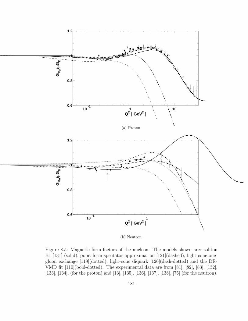
0.6
0.8
1
1.2
10-1
1 10Q2 [ GeV2 ]
GM
p/µ
GD
(a) Proton.
0.6
0.8
1
1.2
10-1
1Q2 [ GeV2 ]
GM
n/µ
GD
(b) Neutron.
Figure 8.5: Magnetic form factors of the nucleon. The models shown are: solitonB1 [131] (solid), point-form spectator approximation [121](dashed), light-cone one-gluon exchange [119](dotted), light-cone diquark [126](dash-dotted) and the DR-VMD fit [110](bold-dotted). The experimental data are from [81], [82], [83], [132],[133], [134], (for the proton) and [13], [135], [136], [137], [138], [75] (for the neutron).
181

0
1
1 2 3 4 5 6 7 8
Q2 [ GeV2 ]
µGE
p/G
Mp
Figure 8.6: The GE/GM ratio for the proton. Open symbols are Rosenbluth data[81], [133], [134], [139], filled symbols are polarized data [90], [140] . Models are thesame as in Figure 8.5.
0
0.05
0.1
0 0.2 0.4 0.6 0.8 1 1.2 1.4 1.6 1.8 2
Q2 [ GeV2 ]
GE
n
Figure 8.7: The electric form factor of the neutron. The E93-026 2001 run resultsare shown with red stars. Other data are: open squares – analysis of the deuteronquadrupole form factor [22], filled circles – recoil polarization [25], [141], [27], filled
squares – ~He3target [31], [33], filled triangles – ~d target [35], [34]. Models are the
same as in Figure 8.5.
182

Chapter 9
Discussion
As we have seen in the previous two sections, the results of the present experi-
ment, as well as those of other recent experiments, can be described by a simple
parametrization (7.10). This gives us confidence that the formalism employed by
the experimental methods is adequate (at least in this kinematic regime) and the
measurements are free of major problems.
This consistency is especially important in light of the recent controversy for
the charge form factor of the proton, where the disagreement between the Rosen-
bluth and polarization measurements is interpreted by many theorists as an evidence
of the two-photon exchange. If the importance of the two-photon exchange contri-
bution is confirmed, the entire formalism of the electron-nucleon scattering will be
challenged (for example, it will be longer possible to represent the electromagnetic
structure of the nucleon in terms of just two form factors [94]).
Unfortunately, the accurate GnE data is only available up to the region where
the Rosenbluth and polarized results for the proton begin to diverge. More accurate
183

data taken with several approaches is needed at Q2 ≥ 2GeV/c2.
The Galster parametrization (7.10) has been traditionally considered as having
no fundamental physical significance. Recently, Kaskulov [142] has shown that
under some approximations GnE can be obtained as:
GnE(Q
2) =〈r2〉n6
Q2Fπ(Q2)GD(Q
2), (9.1)
where Fπ(Q2) is the form factor of the pion, which has monopole Q2-dependence.
The parametrization (9.1) is of the same form as the Galster fit (7.10). Therefore,
the success of the Galster form at low Q2 can be considered as a manifestation of
the chiral content of the nucleon. For higher Q2, exchange currents are expected to
become important.
A careful examination of Figure 7.15 shows that the Galster parameterization
is less successful at Q2 < 0.4 GeV/c2 than elsewhere. The fact that it is hard to keep
the nuclear corrections under control for lower Q2, and the large error bars at this
kinematics, preclude any definitive conclusions. However, if one believes that the
grouping of these data above the Galster line is neither coincidental nor due to some
common flaw in the data analysis, then one can see that the GnE database can be
better fitted with a superposition of a broad Galster-like fit and a low-Q2 “bump”.
Such an ansatz was made by Friedrich and Walcher [143]. They convincingly argue
that the “bump” can be identified with the pion cloud, which reaches as far out as
2 fm, whereas the broader part corresponds to the constituent quark dynamics. The
184
authors stress the need for accurate data at moderate Q2 to test their hypothesis.
Even though none of the QCD-inspired models considered in the previous
chapter provides a complete description for all four electromagnetic form factors
within the entire experimental range, it should be noted that all of them successfully
reproduce the most essential features of the data: the dipole behavior of the magnetic
form factors at modest Q2 and positive non-zero GnE. Non-relativistic SU(6) models
could not recover these features, and thus one can conclude that both relativistic
effects and dynamical SU(6) breaking via spin-dependent quark-quark interaction
are important for understanding the electromagnetic structure of the nucleon.
The results of the presented experiment and another recent JLab experiment
[27] had an appreciable impact on the extracted charge density of the neutron [5]
(see Figure 9.1). One distinctive new feature of the updated densities is a positive
bump at about 1-1.5 fm, which is not consistent with the traditional interpretation
of the charge distribution neutron in terms of a positive core and a negative pion
cloud. The author states that this is a stable and model-independent feature of the
analysis which cannot be eliminated without damaging the quality of the form factor
fits at Q2 ∼ 1 GeV/c2. As suggested by the author, such oscillatory behavior of
the charge density may be a signature of the d-state component of the wavefunction
which is probably broader spatially than that of the s-state.
Recent accurate measurements of GnE with the polarized target had a pro-
nounced positive impact on our understanding of the electromagnetic structure of
185

the nucleon. It could be of interest to apply this experimental method to the proton
form factors. Measuring GpE/G
pM with a polarized target could not only help to
resolve the controversy between Rosenbluth and polarized data, but also provide
useful information for quantitative studies of the effects two gamma exchange if the
latter are found to be of significance. In that case, extraction of the three form
factors (traditional GE,M and the one associated with the two photon exchange)
will require measurements with two or more independent experimental methods.
186

Figure 9.1: Charge and magnetization densities of the neutron. Top panel: GEn data
used in the extraction. Recent JLab data points (the present experiment and [27])are shown in red. Bottom panel: extracted charge densities before (blue hatches)and after (grey hatches) the recent JLab measurements.
187

Chapter 10
Summary and outlook
In the experiment described here (JLab E93-026) the charge form factor of the
neutron was measured at Q2 = 0.5 and 1.0 (GeV/c)2. The data analysis for Q2 = 1.0
was discussed. The result is:
GnE(Q
2 = 1.0) = 0.0454± 0.0054(stat)± 0.0037(sys). (10.1)
This data point is the highest Q2 datum measured with a polarized target. To-
gether with another recently published JLab experiment (E93-038), this experiment
provides the only accurate direct measurements of GnE at Q2 > 1.0 (GeV/c)2.
The theoretical calculations used in the extraction of GnE included the rela-
tivistic effects as well as contributions from meson exchange currents, isobar config-
urations and final state interactions. Studies of the reaction mechanism dependence
confirm the prediction of the Arenhovel’s model [36] that the sensitivity of this
method of measurement to meson exchange currents and the final state interactions
is small (2% and 5% respectively) and decreases with the increase of Q2.
188

Based on our and other experimental results, an improved Galster parametriza-
tion was suggested:
GnE =
0.86µnτ
1 + 3.06τ(1 +Q2/0.71)−2, (10.2)
where as usual τ = Q2/4m2 and the units of Q2 are assumed to be (GeV/c)2.
Our experimental results are consistent with the recoil polarimetry measure-
ment by Madey et al. and the deuteron quadrupole form factor analysis by Sick and
Schiavilla.
The experiment E93-026 has been a part of massive experimental program at
the JLab and other nuclear facilities (NIKHEF, MAMI, MIT-Bates) aiming at im-
provement of our knowledge of the electromagnetic structure of the neutron. Thanks
to this ongoing effort by many experimentalists, the typical uncertainties in GnE have
been reduced from 30 − 40% ten years ago to 10%. The situation will be further
improved upon completion of two other experiments. The JLab experiment E02-013
will extend our knowledge of GnE to higher Q2, whereas the BLAST experiment at
MIT-Bates will improve the accuracy of the world GnE database at low and interme-
diate Q2.
189

Appendix A
Principles of operation of theE93026 polarized target
A.1 Dynamic nuclear polarization
Unpaired nuclear spins align with the direction of the external magnetic field. There-
fore, the simplest method of polarizing a material is by placing it into a strong mag-
netic field. Statistical physics gives the relation between the polarization and spin
J of the nucleus as follows [50]:
P =2J + 1
2Jcoth
(
2J + 1
2J
µB
kT−)
− 1
2Jcoth
(
1
2J
µB
kT
)
, (A.1)
where µ is the magnetic moment of the nucleus, B is the magnetic field, T is the
spin temperature 1 and k is the Boltzmann’s constant.
For the particular case of a spin-1 system this expression simplifies to:
1In thermal equilibrium the spin temperature is equivalent to the temperature of the system.
190

P =4 tanh(µB/2kT )
3 + tanh2(µB/3kT ).(A.2)
For realistic experimental values of B and T the nuclear polarization is low.
For example, for the values of this experiment, B = 5 Tesla and T = 1 K, the
deuteron thermal polarization is only 0.14%. However, the electron polarization
is very high (99.8%), and this high polarization can be transferred to nuclei using
mechanism which bears name of dynamic nuclear polarization (DNP).
Let us consider how DNP works in NH3 targets2. When the material is placed
in a magnetic field, degeneration in m, the quantum number for projection of spin
onto the field direction, is lifted due to Zeeman terms of the Hamiltonian. The
energy eigenstates are pure spin states.
If then the material is doped with paramagnetic radicals, providing free elec-
trons, the spin-spin interaction with unpaired electron spins makes nucleon energy
eigenstates mixed spin states (Figure A.1):
|e ↓ N ↑〉 → |1〉 = |e ↓ N ↑〉+ ε1|e ↓ N ↓〉 (A.3)
|e ↓ N ↓〉 → |2〉 = |e ↓ N ↓〉+ ε?1|e ↓ N ↑〉 (A.4)
|e ↑ N ↑〉 → |3〉 = |e ↑ N ↑〉+ ε2|e ↑ N ↓〉 (A.5)
2ND3 is more complicated due to quadrupole moment and higher spin of deuteron, but allessential features are the same.
191

|e ↑ N ↓〉 → |4〉 = |e ↑ N ↓〉+ ε?2|e ↑ N ↑〉, (A.6)
where mixing coefficients ε1,2 are small (|ε1,2| ¿ 1).
The double-flip transitions, forbidden in the absence of the spin-spin inter-
action due to dipole selection rules, are now allowed. By bombarding the material
with photons of frequency (µe+µN)B/h it is possible to cause transitions from state
|2〉 (nucleon spin anti-aligned) to state |3〉. Since electron relaxation time is small
(a few orders of magnitudes larger than that of nucleons), this transition is almost
immediately followed by a decay of the |3〉 to a |1〉. As a result, the positive polar-
ization of the material is increased. In exactly the same way a negative polarization
of material can be achieved by using photons of frequency (µe + µNB)/h.
The polarization is further enhanced by a mechanism, known as spin diffu-
sion. In this process the nuclear polarization is transferred to neighboring nuclei via
dipole-dipole coupling.
A.2 NMR polarization measurement
NMR system
The target polarization was measured using NMR technique [144]. The idea of the
method is based on the fact that the polarization of a material placed in a varying
magnetic field of frequency ω is related to the absorptive part of the magnetic
susceptibility of the material [144]:
192

|e ↓ N ↑〉
|4〉 ≈ |e ↑ N ↑〉
|e ↑ N ↑〉
|e ↓ N ↓〉
|1 >≈ |e ↓ N ↑〉
|3〉 ≈ |e ↑ N ↓〉
s-s interaction OFF s-s interaction ON
|e ↑ N ↓〉
|2 >≈ |e ↓ N ↓〉
Figure A.1: The effect of spin-spin interaction on levels and states of an electron-nucleon system in an external magnetic field. On the left: pure spin levels inabsence of spin-spin interaction. On the right: spin-spin interaction shifts the energylevels and mixes pure spin states, making previously forbidden double-flip transitionsallowed.
P =2
µ0π~γ2NJ
∫ ∞
0
χ′′(ω)dω, (A.7)
193
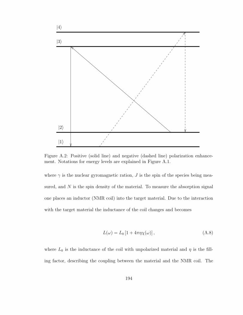
|1〉
|2〉
|3〉
|4〉
Figure A.2: Positive (solid line) and negative (dashed line) polarization enhance-ment. Notations for energy levels are explained in Figure A.1.
where γ is the nuclear gyromagnetic ration, J is the spin of the species being mea-
sured, and N is the spin density of the material. To measure the absorption signal
one places an inductor (NMR coil) into the target material. Due to the interaction
with the target material the inductance of the coil changes and becomes
L(ω) = L0 [1 + 4πηχ(ω)] , (A.8)
where L0 is the inductance of the coil with unpolarized material and η is the fill-
ing factor, describing the coupling between the material and the NMR coil. The
194
impedance of the coil is in its turn measured by including the coil into a resonant
LCR circuit tuned to the Larmor frequency of the deuteron.
195

Appendix B
Measuring beam polarization withthe Hall C Møller polarimeter
Møller measurements employ polarized electron-electron scattering for determina-
tion of the beam polarization. Since Møller scattering is a pure QED process, the
analyzing power can be calculated to a very high accuracy, thus makes possible very
accurate polarization measurements.
For the longitudinal polarization of both beam (Pb) and target (Pt) spins the
scattering cross-section in the center-of-mass quantities is [47]:
dσ
dΩ=
(
dσ
dΩ
)
0
]1 + PtPbAzz(θ)], (B.1)
where ( dσdΩ)0 = (α(3+cos2 θ)/(2E sin2 θ))2 is the unpolarized scattering cross section,
α is the fine structure constant, E and θ are the incident electron energy and the
scattering angle in the center-of-mass frame, and Azz(θ) = − sin2 θ(8− sin2 θ)/(4−
sin2 θ)2 is the analyzing power. The analyzing power reaches a maximum of − 79at
90. Therefore, the detectors are arranged such that to emphasize this kinematic
196

region. The Azz needs to be corrected for the Levchuk effect [145] which takes into
account the initial motion of the atomic electrons.
The Equation B.2 gives the expression for the beam-target asymmetry:
ε =N+ −N−N+ +N−
= AzzPbPt, (B.2)
which can be rewritten for the beam polarization as follows:
Pb =ε
AzzPt
. (B.3)
Here Azz is the acceptance averaged analyzing power. From the Equation B.3 one
can see that the error on the beam polarization has statistical contributions from
the Møller counts and Monte Carlo statistics, and a systematic contribution (Monte
Carlo systematics and the target polarization).
The systematic error is dominated by the Levchuk effect, which is 10% rela-
tive with the size of the effect about 3%, i.e. the contribution is 0.3%. The spin
polarization in iron is known to 0.25%. Other systematic uncertainties (multiple
scattering, beam position and direction, target field value and orientation etc.) are
small (≤ 0.15%). The overall systematic error was found to be 0.47% [47].
197

Bibliography
[1] F. Cardarelli and S. Simula, Phys. Rev. C62, 065201 (2000).
[2] J. Kelly, Advances in Nuclear Physics 23, 75 (1996).
[3] R. Sachs, Phys. Rev. 126, 2256 (1962).
[4] A. W. Thomas and W. Weise, The Structure of the Nucleon (Wiley-VCH,
Berlin, 2001).
[5] J. J. Kelly, Phys. Rev. C66, 065203 (2002).
[6] X. Ji, Phys. Lett. B254, 456 (1991).
[7] G. Holzwarth, Z. Phys. A356, 339 (1996).
[8] A. Licht and A. Pagnamenta, Phys. Rev. D2, 1156 (1970).
[9] A. Mitra and I. Kumari, Phys. Rev. D15, 261 (1977).
[10] S. Kopecky et al., Phys. Rev. Lett. 74, 2427 (1995).
[11] N. Isgur, Phys. Rev. Lett. 83, 272 (1999).
[12] R. Hofstadter and C. de Vries, Phys. Rev. Lett. 6, 290 (1961).
198

[13] A. Lung et al., Phys. Rev. Lett. 70, 718 (1993).
[14] W. Bartel et al., Phys. Lett. 39B, 407 (1972).
[15] K. Hanson et al., Phys. Rev. D8, 753 (1973).
[16] S. Galster et al., Nucl. Phys. B32, 221 (1971).
[17] D. Drickey and L. Hand, Phys. Rev. Lett. 9, 521 (1962).
[18] B. Grossetete, Phys. Rev. 141, (1966).
[19] D. Benaksas, Phys. Rev. 148, 1327 (1966).
[20] G. Simon et al., Nucl. Phys. A364, 285 (1981).
[21] S. Platchkov et al., Nucl. Phys. A508, 343 (1990).
[22] R. Schiavilla and I. Sick, Phys. Rev. C64, 041002 .
[23] G. Hoehler et al., Phys. Rev. Lett. B114, 505 (1976).
[24] N. Dombey, Rev. Mod. Phys. (1969).
[25] T. Eden et al., Phys. Rev. C50, R1749 (1994).
[26] C. Herberg et al., Eur. Phys. J. A5, 131 (1999).
[27] R. Madey et al., Phys. Rev. Lett. 91, 122002 (2003).
[28] B. Blankleider and R. Woloshyn, Phys. Rev. C29, 538 .
199
[29] M. Meyerhoff et al., Phys. Lett. B327, 201 (1994).
[30] J. Becker et al., Eur. Phys. J. A6, 329 (1999).
[31] J. Golak et al., Phys. Rev. 63, 034006 (2001).
[32] D. Rohe, Phys. Rev. Lett. 83, 4257 (1999).
[33] J. Bermuth et al., Phys. Lett. B564, 199 (2003).
[34] H. Zhu et al., Phys. Rev. Lett. 87, 1 (2001).
[35] Passchier et al., Phys. Rev. Lett. 82, 4988 (1999).
[36] H. Arenhovel, W. Leidemann, and E. Tomusiak, Phys. Rev. C46, 455 (1992).
[37] H. Arenhovel, private communication.
[38] W. Fabian and H. Arenhovel, Nucl. Phys. A314, 253 (1979).
[39] H. Arenhovel et al., Phys. Rev. C61, 034002 (2000).
[40] H. Zhu, Ph.D. thesis, University of Virginia, 2000.
[41] C. M. Harris, Ph.D. thesis, University of Virginia, 2001.
[42] C. Sinclair, Technical Report No. TN-97-021, TJNAF (unpublished).
[43] C. Yan, P. Adderley, et al., Nucl. Inst. Meth. A365, 261 (1995).
[44] D. Neuffer, C. Yan, and R. Carlini, Technical Report No. TN-92-054, TJNAF
(unpublished).
200

[45] P. Gueye, E. Joe, and R. Wallace, Status of the actual beam position monitors
in the Hall C beamline, TJNAF Technical Report, 1995, unpublished.
[46] D. Mack, private communication.
[47] M. Hauger et al., nucl-ex/9910013, 1999.
[48] C. Yan, Technical Report No. TN-97-004, TJNAF (unpublished).
[49] C. Yan, Technical Report No. TN-97-036, TJNAF (unpublished).
[50] P. McKee, Ph.D. thesis, University of Virginia, 2000.
[51] D. Crabb and D. Day, Nucl. Instr. Meth. A356, 9 (1995).
[52] P. McKee, Offline target polarization analysis, TJNAF Technical Report, un-
published.
[53] P. Mckee, in Proceedings of the 15th International Spin Physics Symposium
(World Scientific, Singapore, 2002), to be published.
[54] H. Mkrtchyan, Laser Pulser Gain Monitoring System in Hall C, TJNAF Tech-
nical Report, unpublished.
[55] G. Warren, Neutron detector gain matching with cosmics, TJNAF Technical
Report, 1998, unpublished.
[56] J. R. Arrington, Ph.D. thesis, California Institute of Technology, 1998.
[57] CEBAF On-line Data Acquisition, CEBAF, 1993.
201
[58] F. Wesselmann, Gen01 syncfilter preprocessor, TJNAF Technical Report, un-
published.
[59] S. Wood, The CEBAF Test Package: A Symbolic and Dynamic Test, His-
togram, and Parameter Package for On- and Off-line Particle Physics Data
Analysis, TJNAF Technical Report, unpublished.
[60] D. Dutta, Ph.D. thesis, Northwestern Univeristy, 1999.
[61] J. Lightbody and J. O’Connel, Computers in Physics 57 (1988).
[62] F. Krautschneider, Ph.D. thesis, Bonne University, 1976.
[63] M. Frodyma et al., Phys. Rev. C 47, 1599 .
[64] S. Stein, E. Bloom, et al., Phys. Rev. D 12, 1884 (1975).
[65] L. Mo and Y. Tsai, Rev. Mod. Phys. 41, (1969).
[66] D. Day et al., Phys. Rev. Lett. 59, 427 (1987).
[67] L. B. Weinstein, Ph.D. thesis, Massachusets Institute of Technology, 1988.
[68] T. De Forest, Nucl. Phys. A392, 232 (1983).
[69] V. P. R. Schiavilla and R. Wiringa, Nucl. Phys. A449, 219 (1986).
[70] P. Ulmer, MCEEP: Monte Carlo for Electro-Nuclear Coincidence Experi-
ments, version 3.5 ed., Old Dominion University, 2000.
202
[71] R. Madey et al., Nucl. Inst. Meth. 161, 439 (1979).
[72] R. Brun, O. Couet, C. Vandoni, and P. Zanarini, PAW Users Guide, Program
Library Y250 (CERN, Geneva, 1991).
[73] G. Kubon, Ph.D. thesis, University Basel, 1999.
[74] M. Zeier, Contamination by multi step reactions in GEn01, TJNAF Technical
Report, 2003, unpublished.
[75] G. Kubon, Phys. Lett. B524, 26 (2002).
[76] S. Brodksy and G. Farrar, Phys. Rev. D11, 1309 (1975).
[77] P. G. Lepage and S. J. Brodsky, Phys. Rev. D22, 2157 (1980).
[78] M. Burkardt, X. Ji, and F. Yuan, Nucl. Phys. B652, 383 .
[79] A. Belitsky, X. Ji, and F. Yuan, Phys. Rev. Lett. 91, 092003 (2003).
[80] G. Lepage and S. Brodsky, Phys. Rev. Lett. 43, 545 (1979).
[81] L. Andivahis, Phys. Rev. D50, 5491 (1994).
[82] R. Walker et al., Phys. Rev. D49, 5671 (1994).
[83] A. Sill et al., Phys. Rev. D48, 29 (1993).
[84] P. Bosted et al., Phys. Rev. Lett. 68, 3841 (1992).
[85] P. Bosted et al., Phys. Rev. C42, 38 (1990).
203
[86] R. Walker et al., Phys. Lett. B224, 353 (1989).
[87] N. Isgur and C. Llewelyn Smith, Phys. Rev. Lett. 52, 1080 (1984).
[88] C. E. Carlson and F. Gross, Physical Review D36, 2060 .
[89] V. Punjabi et al., nucl-ex/0307001.
[90] O. Gayou et al., Phys. Rev. Lett. 88, 092301 (2002).
[91] O. Gayou et al., Phys. Rev. C64, 038202 (2001).
[92] J. Arrington, Phys. Rev. C68, 034325 (2003).
[93] P. Blunden, W. Melnitchouk, and J. Tjon, Phys. Rev. Lett. 91, 142304 (2003).
[94] P. Guichon and M. Vanderhaeghen, Phys. Rev. Lett. 91, 142303 (2003).
[95] J. Ralston and P. Jain, hep-ph/0302043.
[96] V. Chernyak, hep-ph/9906387v2.
[97] J. Ralston and P. Jain, hep-ph/9212243.
[98] G. Miller, Phys. Rev C66, 065205 (2002).
[99] V. Braun et al., Nucl. Phys. B589, 381 (2000).
[100] P. Mergell, U.-G. Meißner, and D. Drechsel, Nucl. Phys. A596, 367 .
[101] W. R. Frazer and J. R. Fulco, Phys. Rev. 117, 1603 .
204

[102] J. Sakurai, Currents and mesons (University of Chicago Press, Chicago, 1969).
[103] Y. Nambu, Phys. Rev. 106, 1366 (1957).
[104] M. Gari and W. Krumpelmann, Z. Phys. A 322, 689 (1985).
[105] S. Okubo, Phys. Lett. 5, 165 (1963).
[106] G. Zweig, CERN Report Nos. TH-401 and TH-412, 1964.
[107] J. Iizuka, Prog. Theor. Phys. Suppl. 37-38, 21 (1966).
[108] J. Iizuka et al., Prog. Theor. Phys. 35, 1061 (1966).
[109] M. Gari and W. Krumpelmann, Phys. Lett. B 274, 159 (1992).
[110] E. L. Lomon, Phys. Rev. C64, 035204 .
[111] M. Gell-Mann, Phys. Lett. 8, 214 (1964).
[112] K. Barnes, P. Carruthers, and F. von Hippel, Phys. Rev. Lett. 14, 82 (1965).
[113] N. Isgur, G. Karl, and D. Sprung, Phys. Rev. D23, 163 (1981).
[114] P. Dirac, Rev. Mod. Phys. 21, 392 (1949).
[115] V. Berestetskiy and M. Terentiev, Sov. J. Nucl. Phys. 25, 347 (1977).
[116] P. Chung and F. Coester, Phys. Rev. D44, 229 (1991).
[117] S. Brodsky et al., in Particles and fields 2, edited by A. Capri and A. Kamal
(Plenum, New York, 1983), p. 143.
205
[118] F. Cardarelli and S. Simula, Phys. Lett. B467, 1 (1999).
[119] S. Simula, nucl-th/0105024.
[120] S. Capstick and N. Isgur, Phys. Rev. 34, 2808 (1986).
[121] R. Wagenbrunn, B. S., K. W., et al., Phys. Lett. B511, 33 (2001).
[122] Y. Suzuki and K. Varga, Stochastic Variational Approach to Quantum-
Mechanical Few-Body Problems (Springer-Verlag, Berlin, 1998).
[123] M. Anselmino, P. Kroll, and B. Pire, Z. Phys. C36, 89 (1987).
[124] J. Bjorken and S. Drell, Relativistic Quantum Mechanics (McGraw-Hill, New
York, 1964).
[125] P. Kroll, M. Schurmann, and W. Schweiger, Z. Phys. A 338, 339 (1991).
[126] B.-Q. Ma, D. Qing, and I. Schmidt, Phys. Rev. C65, 035205 (2002).
[127] D. Ahluwalia and M. Sawicki, Phys. Rev. D47, 299 (1993).
[128] T. H. R. Skyrme, Nucl. Phys. 31, 556 (1962).
[129] G. Adkins, C. Nappi, and E. Witten, Nucl. Phys. B228, 552 (1983).
[130] E. Braaten, S.-M. Tse, and C. Willcox, Phys. Rev. Lett. 56, 2008 (1986).
[131] G. Holzwarth, hep-ph/0201138.
[132] T. Janssens et al., Phys. Rev. 142, (1966).
206
[133] C. Berger et al., Phys. Lett. B35, 87 (1971).
[134] W. Bartel et al., Nucl. Phys. B58, 429 (1973).
[135] P. Markowitz et al., Phys. Rev. 48, R5 (1993).
[136] H. Anklin et al., Phys. Lett. B336, 313 (1994).
[137] H. Anklin et al., Phys. Lett. B428, 248 (1998).
[138] W. Xu et al., Phys. Rev. Lett. 85, 2900 (2000).
[139] J. Litt et al., Phys. Lett. 31, 40 (1970).
[140] M. Jones et al., Phys. Rev. Lett. 84, 1398 (2000).
[141] M. Ostrick et al., Phys. Rev. Lett. 83, 276 (1999).
[142] M. M. Kaskulov and P. Grabmayr, nucl-th/0308015v1.
[143] J. Friedrich and T. Walker, hep-ph/0303054v2.
[144] B. Adeva et al., Nucl. Instr. and Meth. A349, 334 (1994).
[145] L. Levchuk, Nucl. Instr. and Meth. A394, 496 (1994).
207