Embed Size (px)
Citation preview
ABSTRACT
Title of Thesis: PREDICTING SMOKE DETECTOR RESPONSE USING A
QUANTITATIVE SALT-WATER MODELING TECHNIQUE
Sean Phillip Jankiewicz, Master of Sciences, 2004
Thesis Directed By: Professor André W. Marshall
Department of Fire Protection Engineering
This investigation provides a detailed analysis of the hydraulic analogue technique used
as a predictive tool for understanding smoke detector response within a complex
enclosure. There currently exists no collectively accepted method for predicting the
response of smoke detectors; one of the most important elements in life safety. A
quantitative technique has been developed using salt-water modeling and planar laser
induced fluorescence (PLIF) diagnostics. The non-intrusive diagnostic technique is used
to temporally and spatially characterize the dispersion of a buoyant plume within a 1/7th

scale room-corridor-room enclosure. This configuration is geometrically similar to a full-
scale fire test facility, where local conditions were characterized near five ionization type
smoke detectors placed throughout the enclosure. The full-scale fire and salt-water model
results were scaled using the fundamental equations that govern dispersion. An
evaluation of the local conditions and dispersive event times for both systems was used to
formulate a preliminary predictive detector response model for use with the hydraulic
analogue.
PREDICTING SMOKE DETECTOR RESPONSE USING A QUANTITATIVE
SALT-WATER MODELING TECHNIQUE
by
Sean Phillip Jankiewicz
Thesis submitted to the Faculty of the Graduate School of the University of Maryland, College Park in partial fulfillment
of the requirements for the degree Master of Science
2004 Advisory Committee: Professor André W. Marshall, Chair Professor Richard J. Roby Professor James G. Quintiere Professor Arnaud Trouvé


Acknowledgements
The work presented in this Master’s Thesis was fully funded by Combustion Science and
Engineering, Inc. in Columbia Maryland. I wanted to thank Richard Roby, Mike Klassen,
and the rest of the Combustion Science team for this great opportunity to expand my
knowledge; you all will never be forgotten. I would like to thank Professor André
Marshall, my advisor, mentor, and friend. Not only did Dr. Marshal spend countless
hours with me in the lab but also his guidance, knowledge and support allowed me to
overcome several obstacles and acquire a vast array of knowledge throughout the
completion of this work.
I would also like to extend a note of gratitude to the rest of my thesis committee,
Professor Richard Roby, Professor James Quintiere, and Professor Arnaud Trouvé. The
support from each member of my committee has truly been appreciated. A special thanks
is in order for Xiaobo Yao for his aid in this research, without his help I don’t know
how this project could have been completed. In addition I would like to thank my family
for providing a strong foundation for learning and assisting me in more ways then can be
expressed throughout my colligate experience. Last but not least, I would like to thank
my loving girlfriend Heather Martin, for her immeasurable emotional support throughout
this research. Thank you all for helping me get through this.
ii

Table of Contents List of Tables................................................................................................................... v List of Figures ................................................................................................................ vi Chapter 1. Introduction................................................................................................. 1
1.1 Overview................................................................................................................... 1 1.2 Literature Review...................................................................................................... 6 1.3 Research Objectives................................................................................................ 13
Chapter 2. Scaling ........................................................................................................ 15
2.1 Appropriate Scales for Fire / Salt-Water Analogy.................................................. 16 2.1.1 Determination of the Velocity Scale................................................................ 16 2.1.2 Source Based Scaling for Fires ........................................................................ 17 2.1.3 Source Based Scaling for Salt-Water Analog.................................................. 20
2.2 Dimensionless Equations for Fire / Salt-Water Analogy........................................ 23 2.2.1 Governing Equations for the Fire Flow ........................................................... 23 2.2.2 Governing Equations for the Salt-Water Flow ................................................ 28
Chapter 3. Experimental Approach ......................................................................... 32
3.1 Experimental Test Facility...................................................................................... 32 3.1.1 Gravity Feed System........................................................................................ 33 3.1.2 Model Description ........................................................................................... 35 3.1.3 Injection System............................................................................................... 36 3.1.4 Recirculation System ....................................................................................... 37 3.1.5 Positioning System........................................................................................... 38 3.1.6 Optics ............................................................................................................... 38 3.1.7 Image Acquisition............................................................................................ 41
3.2 Quantitative Methodology ...................................................................................... 41 3.2.1 Injection Consideration.................................................................................... 41 3.2.2 PLIF Requirements .......................................................................................... 44 3.2.3 Optimizing Image Quality ............................................................................... 47 3.2.4 Light Sheet Distribution................................................................................... 50 3.2.5 Converting Light Intensity Measurements to Salt Mass Fraction, Ysalt ........... 51
3.3 Experimental Procedure.......................................................................................... 54 Chapter 4. Analysis...................................................................................................... 55
4.1 Calculating Dimensionless Parameters for Fire Test Data ..................................... 55 4.1.1 Dimensionless Energy Release Rate, Q* ........................................................ 58 4.1.2 Dimensionless Fire Time, t *
fire ......................................................................... 59
4.1.3 Dimensionless Thermal Dispersion Signature, *Tθ .......................................... 59
4.1.4 Converting Optical Measurements to Smoke Mass Fraction, Ysmoke ............... 60
iii
4.1.5 Dimensionless Smoke Dispersion Signature, *smokeθ ........................................ 61
4.2 Calculating Dimensionless Parameters for Salt-Water Model ............................... 62 4.2.1 Dimensionless Salt Mass Flux, *
saltm& ............................................................... 63 4.2.2 Dimensionless Salt-Water Model Time, t *
sw .................................................... 64 4.2.3 Dimensionless Salt Dispersion Signature, *
swθ ................................................ 64 4.3 Converting from Salt-Water to Fire Quantities ...................................................... 65
Chapter 5. Results and Discussion........................................................................... 67
5.1 Salt-Water Dispersion Analysis.............................................................................. 67 5.1.1 Initial Plume and Ceiling Jet............................................................................ 67 5.1.2 Initial Doorway Flow Dynamics...................................................................... 70 5.1.3 Corridor Frontal Flow Dynamics..................................................................... 72 5.1.4 Secondary Doorway Flow Dynamics .............................................................. 74
5.2 Fire Response Time Analysis ................................................................................. 76 5.2.1 Local Conditions at the Time of Alarm ........................................................... 77 5.2.2 Dispersion and Detector Response Times ....................................................... 80
5.3 Predicting Detector Response Time........................................................................ 82 5.3.1 Front Arrival Comparison................................................................................ 83 5.3.2 Activation Lag Time ........................................................................................ 84 5.3.3 Detector Response Time Predictions ............................................................... 85
5.4 Salt-Water and Fire Dispersive Parameter Comparison ......................................... 87 5.4.1 Dispersion Comparison at Activation Time .................................................... 87 5.4.2 Evolving Dispersion Signature Comparison.................................................... 89
Chapter 6. Conclusions............................................................................................... 98 Appendix A: Experimental Results ....................................................................... 100 Appendix B: Check List ........................................................................................... 101 Appendix C: Experimental Procedure .................................................................. 102 Bibliography................................................................................................................ 111
iv

List of Tables
TABLE 1: MORTON LENGTH SCALE FOR SALT-WATER INLET CONDITIONS.......................... 43
TABLE 2: DIMENSIONLESS TURBULENCE CRITERION.......................................................... 44
TABLE 3: PREDICTED DETECTOR RESPONSE TIMES............................................................. 87
TABLE 4: FULL-SCALE FIRE EXPERIMENTAL RESULTS.................................................... 100
TABLE 5: NON-DIMENSIONAL FIRE EXPERIMENTAL RESULTS......................................... 100
TABLE 6: NON-DIMENSIONAL SALT-WATER MODEL EXPERIMENTAL RESULTS.............. 100
v

List of Figures FIGURE 1: ENCLOSURE MODEL AND SMOKE DETECTOR LOCATIONS .................................... 5
FIGURE 2: SCHEMATIC OF THE EXPERIMENTAL TEST FACILITY........................................... 32
FIGURE 3: GRAVITY FEED DELIVERY SYSTEM AND CONTROL VALVE SETUP....................... 34
FIGURE 4: FLOW CONTROL SYSTEM AND METERING DEVICE. ............................................. 34
FIGURE 5: PHOTOGRAPH OF ROOM-CORRIDOR-ROOM MODEL ............................................ 36
FIGURE 6: SALINE SOLUTION INJECTION SYSTEM ............................................................... 37
FIGURE 7: MODEL STAND AND POSITIONING SYSTEM......................................................... 39
FIGURE 8: OPTICAL SET UP ................................................................................................ 39
FIGURE 9: OPTICAL DESCRIPTION OF SPATIAL FILTER ........................................................ 40
FIGURE 10: MAXIMUM INCIDENT PATH LENGTH W/O ABSORBSION .................................... 46
FIGURE 11: LIGHT INTENSITY PROFILE (+/-) CAMERA GAIN ............................................... 48
FIGURE 12: NORMALIZED LIGHT INTENSITY PROFILE (+/-) CAMERA GAIN.......................... 48
FIGURE 13: LIGHT INTENSITY VS. SALT MASS FRACTION................................................... 53
FIGURE 14: LOCAL TFIRE IN FULL-SCALE FIRE EXPERIMENT ................................................ 56
FIGURE 15: LOCAL *Tθ IN FULL-SCALE FIRE EXPERIMENT .................................................. 56
FIGURE 16: LOCAL YSMOKE IN FULL-SCALE FIRE EXPERIMENT.............................................. 57
FIGURE 17: LOCAL *smokeθ IN FULL-SCALE FIRE EXPERIMENT.............................................. 57
FIGURE 18: LOCAL YSALT IN SALT-WATER MODEL............................................................... 62
FIGURE 19: LOCAL *swθ IN SALT-WATER MODEL ................................................................ 63
FIGURE 20: PLANAR SHEET LOCATION #1. ......................................................................... 68
FIGURE 21: PLUMES INTERACTION WITH CEILING (SERIES) ................................................ 69
vi

FIGURE 22: SOURCE ROOM CEILING LAYER / DOORWAY SPILL (SERIES) ............................. 71
FIGURE 23: PLANAR SHEET LOCATION #3. ......................................................................... 72
FIGURE 24: CORRIDOR FLOW DYNAMICS (SERIES) ............................................................. 73
FIGURE 25: PLANAR SHEET LOCATION #4. ......................................................................... 74
FIGURE 26: CORRIDOR TO ADJACENT ROOM DOORWAY SPILL (SERIES).............................. 75
FIGURE 27: ENCLOSURE AND SMOKE DETECTOR LOCATIONS ............................................. 76
FIGURE 28: LOCALIZED GAS TEMPERATURE RISE............................................................... 78
FIGURE 29: LOCALIZED SMOKE MASS FRACTION................................................................ 79
FIGURE 30: CEILING-MOUNTED SMOKE DETECTOR RESPONSE (FIRE) ................................. 81
FIGURE 31: SIDEWALL-MOUNTED SMOKE DETECTOR RESPONSE (FIRE).............................. 81
FIGURE 32: DIMENSIONLESS FRONT ARRIVAL TIME ........................................................... 84
FIGURE 33: DIMENSIONLESS ACTIVATION LAG TIME.......................................................... 85
FIGURE 34: PREDICTED SMOKE DETECTOR RESPONSE TIME ............................................... 86
FIGURE 35: DIMENSIONLESS DISPERSION PARAMETER AT DETECTION ............................... 89
FIGURE 36: EVOLUTION OF DISPERSION (RM1 – C)........................................................... 92
FIGURE 37: EVOLUTION OF DISPERSION (RM1 – S) ........................................................... 93
FIGURE 38: EVOLUTION OF DISPERSION (COR – C)........................................................... 94
FIGURE 39: EVOLUTION OF DISPERSION (COR – S) ........................................................... 97
FIGURE 40: EVOLUTION OF DISPERSION (RM2 - C) ........................................................... 97
vii

Chapter 1. Introduction
1.1 Overview
The prediction of detector response times is an extremely important issue and has been
one of great debate in the field of fire science. From a life safety aspect, it is important to
understand that the majority of fatalities from fire are due to smoke inhalation in areas
that are far from the fire source. Proper detection devices that notify occupants early on
reduce evacuation times and subsequent exposure to hazardous conditions. Smoke
detection devices have slowly evolved with advances in technology. With this evolution
much work has been done to optimize their functionality with the majority of focus being
placed on reducing nuisance alarms. There is ongoing research in determining important
flow properties that govern detection; however accurately predicting detection based on
flow properties is still a challenge. Previous studies have attempted to develop empirical
correlations linking localized gas properties with ionization smoke detector response.
The accuracy of these studies is extremely limited. Furthermore, these studies did little to
advance the current understanding of the physics behind the detection device and it’s
interaction with the surrounding environment. The variables associated with the fuel
type, the specific detection device and its radial distance from the source plume must not
be neglected. Thus, finding a general rule of thumb for determining detector response
times is unlikely.
The response of smoke detectors is strongly governed by the dispersive behavior of the
fire gasses. Characterizing detection behavior is useful for fire analysis and investigation
and improving the performance of detectors. Photoelectric and ionization smoke
1

detectors are the most common detection devices used today and the current study is
limited to the examination of ionization type smoke detectors, due to the limited test data
available. However, the general finding of this work can be extended to include other
types of detectors. The current study uses modeling to assess the practicality of
predicting ionization type detector response times.
For many years, engineers and designers have implemented model studies to predict the
behavior of a physical system of interest.1 The physical system of interest is often called
the prototype. It is understood that there are two objectives in developing a prototype: (i)
to test that we fully understand the fundamentals of the physical process; and (ii) to
provide an alternative to carrying out a large number of expensive, full scale tests to
discover the effect of varying different parameters. For both, it is necessary to check the
results against experimental data.2 There are both analytical (computer) and physical
(laboratory) models that allow such predictions to be made.
Because of the hazardous conditions and inherently destructive nature of fire, models are
used extensively to study fire behavior. Analytical fire modeling includes examples
ranging from complex computational fluid dynamic simulators to simple zone models.
These tools are used to predict the evolution of temperature and smoke conditions within
an enclosure at a fraction of the cost and time associated with full scale fire testing.
Physical modeling is also performed extensively in fire research. Scaled down reacting
experiments of small fires or certain aspects of fires are often studied. Salt-water
modeling is an excellent example of a physical model to study fire induced flows.
2

Previous work has been performed using salt-water introduced into a fresh-water
environment as a means to recreate the buoyant characteristics associated with the flows
of a hot fire plume. Salt-water modeling physically reproduces the dispersion dynamics
related to an adiabatic enclosure fire while allowing experiments to be conducted with
little cost and at a laboratory scale. The current investigation evaluates the strengths and
weaknesses of this technique and the practicality of using this model to characterize the
response of ionization type smoke detectors in a particular fire scenario.
While the development of a valid physical model could prove to be an invaluable tool in
the prediction of smoke dispersion within complex compartments, it is imperative that the
design criteria and limitations be well documented and understood. For the salt-water
model to be considered true, a series of similarity requirements must be met, which
necessitates the matching of non-dimensional groups. Models for which all of the
similarity requirements are not met are called distorted models. Salt-water modeling is
considered a distorted model because many but not all dimensionless groups can be
matched.
For successful use of salt-water modeling as a predictive tool, it is imperative that the
results be interpreted in a manner consistent with the initial design intentions. As with
most models, simplifying assumptions are made with regard to the variables of interest.
Thus, some uncertainty is expected when interpreting results from the model. In the
3

current investigation predictive results are compared to the prototype data, in order to
validate the salt-water model, in an analogous reproduction of the actual experiment.
In this study, a 1/7th scale model is constructed using clear polycarbonate. The model
used in the salt-water experiments is shown in Figure 1. It is geometrically similar to a
full-scale room-corridor-room test facility located at Combustion Science and
Engineering, Inc. in Columbia, MD. The full-scale test facility consisted of two 7.5 ft. by
8.5 ft. rooms connected by a 3.5 ft. by 15 ft. corridor with an enclosure height of 8 ft. The
full-scale tests conducted at this facility included three ceiling and two side wall
ionization type smoke detectors in which the local gas temperature and light obscuration
are measured just outside of each detector.3 The mass loss rate of the fuel is monitored
during testing, along with the smoke detector activation times at each location. In the
current study, the environmental conditions in the full-scale and model enclosures are
evaluated at the detector locations with special attention near the time of alarm. The time
for the initial ceiling jet front to arrive at a given detector and the delay time associated
with the detectors activation is evaluated. This study also examines the trends relating
the detector activation times with the fire dispersion dynamics. Salt-water scale model
experiments are conducted to test the feasibility of using this modeling technique as a
method for predicting smoke detector activation times.
The model is also used in this study to examine the flow characteristics and quantitative
conditions observed in a complex geometry. The salt-water model provides detailed
4

Adjacent Room (RM2)
Source Room (RM1)
COR - S
Corridor (COR)
Figure 1: Arial view of the enclosure model and relocations; dashed lines represent vertical planar lasthe fire or salt-water source location, ● representsdetectors and ■ represents sidewall mounted smok
dispersion data for doorway flows, corridor flows, plume/
general compartment filling. A planar laser induced fluor
technique was used in these salt-water model experiments
The dispersion of salt can be related to the dispersion of h
experiments conducted within this study involve introduci
mixture of salt-water solution and a small quantity of dye.
the fluorescent dye, and the water is homogeneous and oc
the turbulent salt-water flows differential diffusion can be
fluids dilute in the same manner. Thus, the concentration
5
RM1 - C
spective smer slice, ? r ceiling moue detectors
ceiling jet in
escence (PL
to measure
ot gasses an
ng a source
The mixin
curs at the m
neglected s
of dye is dir
RM1 - S
COR - CRM2 - C
oke detepresennted sm
teractio
IF) dia
the dis
d smok
consist
g betwe
olecul
o that th
ectly pr
Slice 2
Slice 3
Slice 4
Slice 5
Slice 1
ector ts oke
n, and
gnostic
persion of salt.
e. The
ing of a
en the salt,
ar level. In
e source
oportional to

the salt-mass fraction within the salt-water, throughout the flow. This source solution is
gently introduced into a fresh water environment within the scale model.
The fluorescent dye becomes chemically excited by passing a laser sheet through the
flow. The excited dye emits light with an intensity that is a direct function of the dye
concentration and the incident laser light. The recorded light intensity, emitted by the
dye, is converted into quantitative salt mass fraction data with the use of digital still
photography and several post processing tools. The technique provides quantitative
spatially and temporally resolved dispersion data within the enclosure.
Digital photography is used to evaluate the PLIF images at various locations of interest
and stages of dispersion. The current study uses the PLIF technique in conjunction with
salt-water modeling to obtain non-intrusive quantitative measurements of the dispersion
dynamics within a complex enclosure. Several planar slices are examined within the
enclosure. Data is recorded for various flow conditions and the results are spatially and
temporally resolved. The experimental data is used to visualize and characterize plume
dispersion throughout the enclosure. Ultimately, a comparison of the salt-water and full-
scale fire experiments is made to evaluate salt-water modeling as a predictive tool for
determining smoke detector activation times.
1.2 Literature Review
The relationship between salt-water movement in fresh water and hot smoke movement
in cool (ambient) air has been a topic of interest for many years in fire science. Several
6

authors have conducted experiments using salt-water modeling as a qualitative technique
in which the flow dynamics of fire induced gasses can be estimated. Thomas et al. used
salt-water to model the effect of vents in the removal of smoke from large
compartments.4 Tangren et al. used salt-water to model the smoke layer migration and
density changes within a small-ventilated compartment.5 Zukoski used salt-water
modeling to aid in the prediction of smoke movement within high-rise buildings.6
Steckler, Baum and Quintiere also used this technique to evaluate smoke movement
within a Navy combat ship.7 The experiments conducted within these studies involved
mixing saline solution with a dark blue dye for better flow visualization. As the dyed
salt-water becomes diluted, which is analogous to air entrainment, the color lightens. The
tracer dye allows visualization of the dispersion dynamics and front movement within an
enclosure. Sequential imaging of the traced dye, allowed the front arrival times and
ceiling layer descent to be examined. This application of salt-water modeling is purely
qualitative and does not allow for concentration measurements within the flow to be
examined in detail.
More precise measurements have been taken by placing a conductivity probe within the
tank at a location of interest. Thus, allowing the salinity of the water to be monitored at a
specified point within the test enclosure. It is important to note that the use of
conductivity probes disturbs the flow field, allows only point measurements to be taken.
There is also a lag time associated with these measurements. Kelly has used this
technique in evaluating the movement of smoke within a two-story compartment, in
which the salt-water front movement is compared to predictions from FDS.8 The study
7

demonstrated that under different flow conditions the analogue results scaled well
internally, as did the FDS results for various fire source strengths. The dispersion
dynamics for both systems suggest that the salt-water analogue is a useful tool for
predicting the front arrival times of the hot gasses produced from a fire. However,
dissimilarity is encountered between the magnitudes of the dimensionless dispersion
parameters for the FDS and salt-water results. Quantitatively, the differences are difficult
to ascertain as a physical analogue model is being compared to an analytical model.
Currently, a quantitative visualization technique called planar laser-induced florescence
(PLIF) is available that allows non-intrusive measurements to be taken within the entire
spatial domain of a planar slice. PLIF is far superior to point measurements because it
reveals the instantaneous spatial relationships that are important for understanding
complex turbulent flows.9 Planar laser induced fluorescence is a diagnostic tool that has
proven to be effective in measuring concentration fields within mixing reactions, to
describe the onset of turbulence in a free air flow and to capture the particular flow
phenomena in wave induced motion, just to state a few examples.10,11, 12 PLIF
diagnostics have recently been used in conjunction with salt-water modeling to better
visualize the dynamics of dispersion. Law & Wang use PLIF and salt-water modeling to
examine of the mixing process associated with turbulent jets and provide insight on the
experimental and calibration techniques.13 Peters et al. describe the bounds associated
with PLIF image processing and temporal averaging while assessing the flow dynamics
of gravity current heads.14 A recent validation study has found good agreement between
results using PLIF in conjunction with salt-water modeling and the hydrodynamic
8

simulator of FDS.15 For the current study this diagnostics technique will be used to
quantitatively measure the dispersive dynamics associated within a complex enclosure.
The validity of the salt-water modeling technique is based on the analogy found between
the equations that represent dispersion of heat and mass for the fire and salt-water cases,
respectively. Baum and Rehim conducted a study on three-dimensional buoyant
plumes in enclosures, in which large-scale transport was calculated directly from
equations of motion.16 Within this study, a previous set of “thermally expandable fluid”
equations developed by the authors was introduced and the Bousinesq transport equations
were derived.17 The derivation of the non-dimensional governing equations for the flow
of in-viscid gas within the enclosure is presented in terms of a fire plume and an injected
salt-water plume. The turbulent dispersion dynamics for the fire and salt-water model are
analogous and are described by the momentum, mass species and energy equations.
Although the mass transport of the salt and dye occurs by molecular diffusion and
turbulent mixing, previous studies have concluded that molecular diffusion is
insignificant compared to turbulent mixing for a flow not-close to boundaries.7 The time
scales associated with the convection-dominated flows are far too small to concern the
effects of the slow diffusion process.14
The salt-water modeling test facility used in this study is concurrently being used to
examine the dynamics associated with turbulent plume dispersion and plume ceiling jet
interactions. Original findings from this work aided in the current study. A detailed
evaluation of the governing equations for the analog also revealed more appropriate
9

scaling parameters for the salt-water equations. The new scaling parameters provide an
improved formulation of the salt-water analogy.18 A detailed dimensional analysis is
provided in the Chapter 3, and the dimensional parameters are computed and presented in
the analysis section of this study.
An extensive examination of the current literature encompassing the use of salt-water
modeling has been conducted for this study, in order to assess the physical and
experimental requirements necessary for the model. Morton et al. describe in detail the
physical parallel that can be ascertained between the injection of salt water and a buoyant
fire plume.19 The gravitational convective or buoyant characteristics maintain the same
general form, provided certain criteria are met. The local changes in density within the
plume must be small when compared to the ambient density. Dai et al. reveal that in
order to maintain the self-preserving behavior of a turbulent plume, the density within the
flow must not be very different from the ambient density, such that
1max <<
−
o
o
ρρρ
where maxρ is the maximum density within cross-section of the flow and oρ is the
surrounding fresh water density.20 This condition is incorporated into the salt-water
model to maintain consistency with classical plume theory. Within the salt-water
analogue, it is also required that the source does not produce an appreciable amount of
momentum at its origin. Morton suggests that the initial momentum of the origin is
unimportant at a distance far from the source in which buoyancy dominates the flow
dynamics.21 This distance is characterized by the Morton length scale
10

( )2/1
24/1
4
−
=
oinj
injoM
gd
udl
ρρ
ρπ
where d is the diameter of the source, g is acceleration due to gravity and is the
injection velocity. For the current study, the Morton length scale is used to determine the
flow conditions necessary to produce a buoyancy dominated plume. The momentum
effects are considered insignificant and the plume becomes buoyancy dominated at a
distance above the source equal to
inju
Ml×5 .21
Past authors have chosen the source strength of the salt-water model to satisfy a critical
Reynolds number criterion. A Re > 104 based on a buoyant velocity scale and enclosure
height has been specified in previous studies to ensure a turbulent flow.7,8,15 The current
study also recognizes the importance of a turbulent flow; however, criterion is specified
based on a critical Grasholf number. A detailed explanation of this criterion and its effect
on the selection of flow conditions is presented in § 3.2.1.
Existing literature demonstrates that salt-water modeling can be a useful tool in
describing the flow conditions brought forth by smoke. With this in mind, it may be
possible to predict detector response times using the salt-water analog. The little work
that has been done in regards to the predictability of smoke detector activation has
attempted to describe a threshold for activation with empirical data.22,23 Until recently the
most commonly accepted engineering approach for predicting the activation times of
smoke detectors used a temperature-based correlation, in which a temperature rise of
13°C in the vicinity of the detector was used to describe smoke detector activation. This
11

approach, initially proposed by Heskestad and Delichatsios, used the temperature
criterion selected from the experimental results of a wide range of fuels and detector
styles in which the values ranged from 2°C to over 20°C.22 Extensions of this work
include investigations of localized temperature and/or light obscuration measurements
outside of a detector at the time of activation.25,26,27,28,29,30 However, neither ionization
nor photoelectric smoke detectors operate based on light obscuration or changes in
temperature.31 Furthermore, the details of these empirical predictions are vague and have
often been found to lack repeatability.27,28,29,32
More advanced studies have been conducted that are more realistic to the operating
principles of ionization smoke detectors. These models have been created to describe a
threshold based on the fuel specific smoke properties, such as particle size and
concentration, and the devices specific entrance dynamics and operational parameters.
The details associated with these predictions are beyond the realm of a practical
engineering model and include inherent errors associated with the measurements
needed.32 Even when considering a fuel with well-documented properties there still exists
a large range in smoke particle sizes (0.005 – 5 µm), smoke concentrations (104 – 1010
particles / cm3) and the effect of smoke aging resulting from particle coagulation and
agglomeration, that makes the above prediction in virtually unobtainable outside a
laboratory environment.33 A recent study conducted by Cleary, et al. focuses on
quantifying the significance of smoke entry lag as a function of the incident ceiling jet
velocity.34 The entry lag is defined as a combination of the delay associated with the
velocity reduction as the smoke enters the sensing chamber (dwell time) and the delay
12

associated with the mixing that occurs in the sensing chamber (mixing time). The entry
lag was determined to be inversely proportional to the velocity for the detectors included
in the study. Though, this work provides a detailed means for better understanding
detector response, it is still a relatively new concept and the general applicability has not
been fully tested.32
The findings and recommendations of previous authors provide a strong foundation for
this study. Salt-water modeling has been successfully used for the past decade as an
analog for the dispersion of hot gasses produced in a fire. While at the same time, one of
the most debatable and significant aspects of fire science are found in evaluating detector
response times, which are strongly governed by the dispersive behavior of the fire gasses.
Yet, no research has been done to evaluate the ability of the salt-water analog to be used
as a predictive tool for determining detector activation times. The current study
incorporates the use of state of the art laser diagnostics with a well-established physical
model to determine the predictive capabilities of salt-water modeling.
1.3 Research Objectives
The primary objective of this study is to examine the use of salt-water modeling as a
predictive tool for determining the response time of ionization type smoke detectors. A
series of reduced-scale salt-water model experiments was used to recreate full-scale fire
tests, which examined the local conditions of five smoke detectors positioned throughout
a complex room-corridor-room enclosure. A planar laser induced fluorescence (PLIF)
diagnostic technique was used in conjunction with salt-water modeling for quantitative
13

non-intrusive planar measurements describing the spatial and temporal dispersion
behavior.
PLIF visualization provides insight into the dispersive details of the fluid in the regions of
interest, i.e. in the vicinity of each detector. The PLIF technique provides opportunity to
visualize the various stages of dispersion including; the initial plume regime, the
impinging plume ceiling interaction, the ceiling layer descent, as well as the doorway and
corridor flow characteristics. A secondary objective of this investigation is to gain
insight into dispersive phenomenon within the enclosure.
In order to achieve the primary objective of this investigation, multiple considerations
must be made regarding the possible conditions governing detector response. The
quantitative capabilities of the PLIF technique are exploited to evaluate the dispersion
signature at select locations. These signatures are taken at locations corresponding to
detector positions in the full-scale fire test. The time evolution of dispersion parameters
from the salt-water model and the full-scale fire are compared with a special focus on the
detector activation event. The dispersion parameters include temperature and smoke
parameters for the fire and a salt parameter for the salt-water model. In addition, a
detailed analysis of the front arrival times for both the full and reduced scale experiments
is conducted based on the dispersion parameters signatures. The trends and relative
values are used to demonstrate the strengths and weaknesses of using salt-water modeling
as a predictive tool for smoke detector response.
14

Chapter 2. Scaling
It has been found, through the use of dimensional analysis that a direct link can be made
between the thermal strength of the source fire and the salt mass strength of the salt-water
source. Assumptions must be made regarding the factors that govern smoke movement
for this analogy to be drawn. The salt-water modeling, or the hydraulic analogue
technique, represents adiabatic fire conditions where buoyancy is the dominating factor in
the migration of smoke within an enclosure. Smoke is dispersed throughout the enclosure
and is driven by the hot gasses that accelerate toward the ceiling in the initial plume
regime. The buoyant force is a result of the density difference between the hot gasses
produced from a fire and the cool ambient environment. Thus, the source strength and the
height of the enclosure dictate the manner in which the dispersion occurs. Similarly, salt-
water is introduced into a freshwater environment where the density difference creates a
buoyant driving force. The plume regime drives the flow with the ceiling height and
source strength controlling the dispersion dynamics within the entire enclosure.
Understanding the equations that govern these dynamics allows the similarities and
differences to be compared for both the fire and salt-water experiments. By scaling the
governing equations, non-dimensional parameters that represent the dispersion dynamics
can be obtained. The following section provides a detailed explanation of the appropriate
dimensionless terms for both the fire and salt-water analogy and incorporates the appropriate
scales intothe governing equations that describe the dispersion dynamics of both systems.
This chapter demonstrates the similarities between the governing equations for these
flows. A detailed explanation of the methods used to compute and visualize dimensionless
variables and parameters for fire analysis is presented in Chapter 4.
15
2.1 Appropriate Scales for Fire / Salt-Water Analogy
2.1.1 Determination of the Velocity Scale
The momentum equation with a Boussinesq treatment of the density is provided as
( ) ( ) jo
ii
j
j
a
i
ji
jo f
xxu
xpp
xu
utu
ρρµρ −+∂∂
∂+
∂−∂
−=
∂
∂+
∂
∂ 2
, (1)
where oρ is the ambient density, u is the velocity vector, is the time, j t p is the pressure,
is the atmospheric pressure, ap µ dynamic viscosity, ρ is the fluid density, and is
the body force.
jf
Let us consider scales of terms in a convective buoyancy dominated flow “not close” to a
boundary described by Eqn. (1). The scales for these terms are
o
ooUτρ
;LU oo
2ρ : Lpo ; 2L
Uoµ; gosource ρρ − ,
where L is the length scale, Uo is the velocity scale, τo is the time scale, is the pressure
scale, g is the gravitational acceleration constant, and is the source pressure scale.
op
sourcep
Assuming transients are governed by a convective time scale, o
o UL
=τ , the terms reduce
to
LU oo
2ρ : Lpo ; 2L
Uoµ; gosource ρρ − .
Because the flow is convective and buoyancy dominated, the convective and buoyancy
terms balance and
16

gLU
osourceoo ρρ
ρ−~
2
.
An appropriate velocity scale for a convective buoyancy dominated flow “not close” to
the boundary is thus
( ) 2/12/1
~ gLUo
osourceo
−
ρρρ
. (2)
It is important to note that if the flow is “close” to the wall, the viscous terms would
become important, the appropriate length scales would chance, and the corresponding
velocity scales would change.
2.1.2 Source Based Scaling for Fires
The scale for Uo is provided in terms of the density deficit, oosource ρρρ − . For fires the
density deficit is not well established and a scale for Uo and other quantities of interest
based on the source strength is more useful. For a fire
( )osourcepfire TTcmQ −&~ (3)
where is a characteristic mass flux from the fire plume source and Tfirem& source is a
characteristic temperature of the fire plume source. Furthermore,
( )
o
osourcepfire
o TTTc
mTQ −
&~ . (4)
A scale for the source can be determined by recognizing
2~ fosourcefire LUm ρ&
or alternatively,
17

2~ fooo
sourcefire LUm ρ
ρρ
& (5)
Where ρsource is the density of the source flow. Substituting Eqn. (5) into Eqn. (4) and
rearranging results in a new expression for the velocity scale:
( ) 11
2~−−
−
o
source
o
osource
fopoo T
TTLTc
QUρ
ρρ
(6)
This velocity expression has the source strength but also a temperature difference term.
More analysis is required to simplify the expression.
For a Boussinesq flow, the density changes are small and a Taylor series expansion can
accurately describe the density. For fires, only the effect of temperature on density is
considered. Composition changes within the fire-induced flow are assumed to have a
negligibly small impact on the density. The density can be expressed as
( ),
Higher order termsTTT o
opo +−
∂∂
+=ρρρ (7)
or
( )[ ] Higher order terms,TT oToo +−−= βρρρ
where Tβ is the volumetric thermal expansion coefficient defined as
TT ∂∂
−=ρ
ρβ 1 .
Furthermore, the fire-induced flow is assumed to behave like an ideal gas so that
RTp
=ρ (8)
and
18

o
o
o
o
op TRTp
Tρρ −
=−
=∂∂
2,
(9)
Combining Eqns. (7) and (9) results in
( )
o
ooo T
TT −−≈ ρρρ (10)
and βT is the volumetric thermal expansion coefficient given by
o
T T1
=β .
The linear expression in Eqn. (10) resulting from the Buossinesq approximation helps to
simplify the scales.
Substitution of Eqn. (10) into Eqn. (6) and only retaining leading order terms results in
( ) 1
2~−
−
o
osource
fopoo T
TTLTc
QUρ
. (11)
Furthermore, a relationship between the density deficit and the dimensionless
temperature difference is provided by Eqn. (10). Substitution results in
( )
o
oo
TTT −
−=−ρρρ
or ( oTo TT −−= )−
βρρρ
. (12)
Applying Eqn. (12) and substituting into Eqn. (11) results in
( ) 1
2~−
−−
o
osource
fopoo LTc
QUρ
ρρρ
. (13)
Combining Eqn. (13) and Eqn. (2) results in an expression relating the density deficit to
the source strength given by
19

( ) ( ) 1
22/1
2/1
~−
−−
−−
o
osource
fopof
o
osource
LTcQgL
ρρρ
ρρρρ
.
Recognizing that ( )osourceosource ρρρρ −−=− for a fire and simplifying results in
( ) ( ) 3/2*~ Q
o
osource
ρρρ −
, (14)
where
= 2/52/1
*
fopo LgTcQQ
ρ.
Substitution of Eqn. (10) into Eqn. (2) results in a scale for Uo in terms of the source
given by
( ) ( ) 2/13/1*~ fo gLQU . (15)
2.1.3 Source Based Scaling for Salt-Water Analog
The scale for Uo is provided in terms of the density deficit, oosource ρρρ − . Although
this quantity can be calculated for salt-water sources, for a completely parallel analogy, a
source-based scale for Uo and other quantities of interest are developed for the salt-water
flow just as for the fire flow. For salt-water flows
( )VYm saltsourcesalt&& ρ= , (16)
where V is the volumetric flow rate of salt-water, Y& salt is the mass fraction of salt in the
injected source flow and is the mass flow rate of salt introduced into the system. saltm&
Alternatively,
20

( )VYm saltoo
sourcesalt
&& ρρ
ρ
= .
An expression for the mass flux of salt can also be given in terms of a characteristic flow
velocity as
( )( saltswooo
sourcesalt YLUm 2~ ρ
ρρ
& ) . (17)
Rearranging results in
( ) 11
2~ −−
salt
o
source
swo
salto Y
LmU
ρρ
ρ&
. (18)
This velocity expression has the source strength, m , but also a salt mass fraction term,
Y
salt&
salt. More analysis is required to simplify the expressions.
For the salt-water flow, an empirical expression for the density of salt-water as a function
of the salt mass fraction has been established as
saltoo Yρρρ 76.0+= .
The expression was determined from existing data. The empirical expression
shows that the salt-water density is a linear function of the salt mass fraction. A first-
order Taylor series expansion of the density about changes in mass fraction will also
provide a linear relationship for density. This expansion provides some physical insight
into the empirical expression. The expansion is given by
( salto
o YY∂∂
+=ρρρ ) , (19)
and similar to the fire case a density modification coefficient, βsw is defined as
21
Ysw ∂∂
=ρ
ρβ 1 . (20)
Substitution of Eqn. (20) into Eqn. (19) and equating results in
saltoswo Yρβρρ += , (21)
where βsw = 0.76. Note the similarity between Eqn. (21) and the expression for
temperature based density in Eqn. (10) recognizing that βT = 1 / To.
Rearranging Eqn. (21) results in
sourceswo
osource Yβρ
ρρ=
− (22)
Comparison of Eqns. (22) and (12) demonstrates the quantities that result in buoyancy for
the fire and the salt-water model. in simulating the buoyant force which drives fire
induced flows. Substitution of Eqn. (21) into Eqn. (18) and retaining only leading order gives
11
2
1~−−
−
o
osource
swswo
sourceo L
mUρ
ρρβρ
& (23)
Combining Eqns. (23) and (2) results in
( )11
22/1
2/11~
−−
−
−
o
osource
swswo
sourcesw
o
osource
LmgL
ρρρ
βρρρρ &
( ) 3/2*~ mo
osource &ρ
ρρ − (24)
where
2/52/1*
swo
sourceswsw Lg
mm
ρβ &
& = (25)
22
( ) 3/2*~ mo
osource &ρ
ρρ − (24)
where
2/52/1*
swo
sourceswsw Lg
mm
ρβ &
& = (25)
Substitution of (24) into (2) results in a velocity scale in terms of the source strength
given by
( ) ( ) 2/13/1*~ swswo gLmU & (26)
2.2 Dimensionless Equations for Fire / Salt-Water Analogy
2.2.1 Governing Equations for the Fire Flow
Momentum Equation:
The momentum equation is given by
( ) ( ) jo
ii
j
j
o
i
ji
jo f
xxu
xpp
xu
ut
uρρµρ −+
∂∂
∂+
∂−∂
−=
∂
∂+
∂
∂ 2
(27)
where
, , 0 03 =f 1 =f gf −=2
Define dimensionless variables as follows
o
firett
τ=ˆ ,
f
jj L
xx =* ,
o
jj U
uu =ˆ ,
o
a
ppp
p−
=ˆ
( )
( ) oosource
oo
ρρρρρρ
θ/
/ˆ−
−= ,
gf
f jj =*
so that
, , 0 0*3 =f *
1 =f 1*2 −=f
23

( ) *
2**
2
*2*ˆˆˆˆ
ˆˆˆ
jo
fosource
ii
j
foioo
o
i
ji
j
oo
f fU
gLxx
uLUx
pUp
xu
ut
uU
L⋅
−+
∂∂
∂+
∂∂
−=∂
∂+
∂
∂θ
ρρρµ
ρτ
We will set
1=oo
f
UL
τ
so that the characteristic development time or transient is based on the flow time. We will
also get
12 =oo
o
Up
ρ
so that the characteristic pressure is based on the flow pressure. Rewriting results in
( ) *
2**
2
**ˆˆˆˆ
ˆˆˆ
jo
fosource
ii
j
foii
ji
j fU
gLxx
uLUx
pxu
ut
u⋅
−+
∂∂
∂+
∂∂
−=∂
∂+
∂
∂θ
ρρρν (28)
The fire induced flow expressions are available in terms of the source strength for U
and (
o
) oosource ρρρ − . These expressions are given by Eqns. (14) and (15). Substitution
of these scale results into expressions for the dimensionless variables in Eqn. (28) gives
( ) ( )
****
*2
2/13/1**
*
*
**
*
*
jTii
j
ffii
ji
j fxx
u
LgLQxp
xu
utu
⋅+∂∂
∂+
∂∂
−=∂
∂+
∂
∂θν
or
( )
****
*2
3/1*
*
*
**
*
* 1jT
ii
j
firesourceii
ji
j fxx
u
Grxp
xu
utu
⋅+∂∂
∂+
∂∂
−=∂
∂+
∂
∂θ (29)
where
firesourcef
po
ff
fopo
GrQgLcT
LLQgLgTc 1
2
2
32/32/3
2/52/13
==νµνρ
or alternatively for an ideal gas
24

3
2
3
2
νρνρβ
opo
f
po
fTfiresource Tc
gQLc
gQLGr == (30)
And the scaled variables in terms of the source terms are
( ) ( ) 3/1*2/1* QLgtt ffirefire ⋅= , ( ) ( ) 2/13/1*
*
f
jj
gLQ
u=u ,
( )( ) 3/2*
*
Q
TT oTT
−=β
θ , ( ) fo gLQ
ppρ
3/2*
* =
where oTT
1=β (31)
Energy Equation:
A dimensionless energy equation is also derived beginning with the energy equation
given by
qxx
TkxTu
tTc
iiiipo ′′′+
∂∂∂
=
∂∂
+∂∂ 2
ρ . (32)
Scale parameters are defined as follows:
o
firett
τ=ˆ ,
f
ii L
xx =* ,
o
ii U
uu =ˆ ,
QLq
q f3
*′′′
=&
& (33)
( )( ) 3/2*
*
Q
TT oTT
−=β
θ .
Substitution of scales results in
( ) ( ) ( ) *
3**
*2
2
3/2*
*
*3/2*0
*3/2*0 ˆ
ˆ qLQ
xxLQk
xu
LUQc
tQc
fii
T
fTi
Ti
fT
opT
oT
p +∂∂
∂=
∂∂
+∂∂ θ
βθ
βρθ
τβρ
.
Rearranging results in
25

( )
*23/2*
0**
*2
*
**
ˆˆ q
LUQc
QLxxLUx
utU
L
fop
fT
ii
T
foi
Ti
T
oo
f
ρβ
θνανθθ
τ+
∂∂∂
=∂∂
+∂∂ . (34)
Just as before
1=oo
f
UL
τ
And the scale for U in Eqn. (15) is set equal to U , the scale for o o ( )oT TT −β is
determined from Eqns. (12) and (14) and set equal to ( )oT TT −β yielding
( )
***
*2
2/12/13/1**
**
*
*
qxxLLgQx
ut ii
T
ffi
Ti
fire
T &+∂∂
∂
=
∂∂
+∂∂ θ
νανθθ
,
or
( )
***
*2
3/1*
**
*
*
Pr11 q
xxGrxu
t ii
Tfire
sourcei
Ti
fire
T &+∂∂
∂
=
∂∂
+∂∂ θθθ
, (35)
where Gr is given in Eqn. (30) and firesource
αν
=Pr .
The scaled variables in terms of the source terms are defined in Eqn. (31).
Smoke Mass Species Equation:
The smoke mass species equation involves generation of smoke due to reaction and
dispersion of smoke due to density differences. The dispersion is primarily associated
with differences in temperature. Consider the mass species equation describing the
dispersion of smoke:
26

smokeii
smokeo
i
smokei
fire
smokeo w
xxY
Dx
Yu
tY
&+∂∂
∂=
∂∂
+∂∂ 2
ρρ , (36)
where Ysmoke is the smoke mass fraction, D is the mass diffusion coefficient, and is
the smoke generation term. Scaling parameters are defined to create a non-dimensional
equation. The non-dimensional equation reveals important dimensionless parameters that
govern the smoke dispersion. Scale parameters are defined as
smokew&
o
firett
τ=ˆ ,
f
ii L
xx =* ,
o
ii U
u=u ,
smoke
fsmokesmoke m
Lww
&
& 3* = ,
Substitution results in
2
*
**
2
*ˆ
ˆfoo
smokesmoke
ii
smoke
foi
smokei
smoke
oo
f
LUmw
xxY
LUD
xYu
tY
UL
ρτ&
+∂∂
∂=
∂∂
+∂
∂ , (37)
In the fire, the velocity scale is given by Eqn. (15).
It should also be recognized that
( )( ) ( )c
smokesmokefuelsmoke H
yQymm∆
== && (38)
Using the characteristic flow time ofo UL /=τ and substituting Eqns. (38) and the fire
velocity scale into Eqn. (37) yields
( )
( ) 2/52/13/1*
*
**
2
**
*fco
smokesmoke
ii
smoke
foi
smokei
smoke
LgQH
yQwxx
YLU
Dx
Yu
tY
∆+
∂∂∂
=∂
∂+
∂∂
ρ.
The source term can be reduced yielding
( ) ( )
( )c
opsmokesmoke
ii
smoke
ffi
smokei
smoke
HTcyQw
xxY
LgLQD
xYu
tY
∆+
∂∂∂
=∂
∂+
∂∂
3/1**
**
2
2/13/1***
* . (39)
A dimensionless smoke dispersion parameter can be defined as
27

( ) 3/2*
*
QTcyHY
opsmoke
csmokesmoke
∆=θ . (40)
Substituting Eqn. (40) into Eqn. (39) results in
( ) ( )
***
*2
2/13/1**
**
*
*
smokeii
smoke
ffi
smokei
smoke wxxLgLQ
Dx
ut
+∂∂
∂=
∂∂
+∂
∂ θθθ .
Recall the definitionGr provided in Eqn. (30). Substitution results in firesource
( )
***
*2
3/1*
**
*
* 1smoke
ii
smokefire
sourcei
smokei
smoke wxxScGrx
ut
+∂∂
∂=
∂∂
+∂
∂ θθθ
The dimensionless variables are
( ) ( ) 2/13/1*
*
/ −−=f
firefire
LgQ
tt ,
( ) ( ) 3/1*2/1*
QgL
uu
f
jj = ,
( ) 3/2*
*
Qcy
YH
psmoke
smokecTsmoke
∆=
βθ
where oTT
1=β .
2.2.2 Governing Equations for the Salt-Water Flow
Momentum Equation:
The momentum equation is given by
( ) ( ) jo
ii
j
j
o
i
ji
jo f
xxu
xpp
xu
ut
uρρµρ −+
∂∂
∂+
∂−∂
−=
∂
∂+
∂
∂ 2
, (41)
where
f1 = 0, f2 = -g, f3 = 0
Define parameters as follows
o
ttτ
=ˆ , sw
jj L
xx =* ,
o
jj U
uu =ˆ ,
o
o
ppp
p−
=* (42)
28

( )
( ) oosource
o
ρρρρρ
θ/
ˆ−−
= , gf
f jj =* so that f1 = 0, f2 = 1, f3 = 0
Substitution of these scales results in
( ) ***
2
2*
*
*
2ˆˆˆ
ˆˆˆ
jo
osource
ii
j
sw
o
jsw
o
i
ji
sw
ooj
o
oo fgxx
uLU
xp
Lxu
uLU
tuU
⋅−
+∂∂
∂+
∂∂
−=∂
∂+
∂
∂θ
ρρρµρρ
τρ
Rearranging results in
( ) *2**
2
2*
*
2*ˆˆˆ
ˆˆˆ
jo
swosource
ii
j
swojoo
o
i
ji
j
oo
sw fU
gLxx
uLUx
pUp
xu
ut
uUL
⋅−
+∂∂
∂+
∂∂
−=∂
∂+
∂
∂θ
ρρρν
ρτ
Just as before
1=oo
sw
ULτ
so that the characteristic development time or transient is based on the flow time. Also,
12 =oo
o
Up
ρ
so that the characteristic pressure is based on the flow pressure. Rewriting results in
( ) *2**
2
*
*
*ˆˆˆ
ˆˆˆ
jo
swosource
ii
j
swoji
ji
j fU
gLxx
uLUx
pxu
ut
u⋅
−+
∂∂
∂+
∂∂
−=∂
∂+
∂
∂θ
ρρρν (43)
For the salt-water flow scales are available in terms of the source strength for U and o
( ) oosource ρρρ − . These expressions are given by Eqn. (24) and Eqn. (26). Substitution
results in
( ) ( )
****
*2
2/13/1**
*
*
*
*
*
ˆ jswii
j
swswswii
ji
j fxx
u
LgLmxp
xu
utu
⋅+∂∂
∂+
∂∂
−=∂
∂+
∂
∂θν
&,
or
29

( )
****
*2
3/1*
*
*
**
*
* 1jsw
ii
j
swsourceii
ji
j fxx
u
Grxp
xu
utu
⋅+∂∂
∂+
∂∂
−=∂
∂+
∂
∂θ , (44)
where
3
2
νρβ
o
swsaltswswsource
gLmGr
&= . (45)
And the scaled variables in terms of the source terms are
( ) ( ) 2/13/1*
*
/ −−=swsw
swsw
Lgm
tt
&,
( ) ( ) 3/1*2/1*
swsw
jj
mgL
u
&=u ,
( ) 3/2*
*
sw
saltswsw
m
Y&
βθ = ,
where 0 76.=swβ . (46)
Salt Mass Species Equation:
The mass species equation for the salt-water flow is
Bii
Bo
i
Bi
Bo w
xxYD
xYu
tY
&+∂∂
∂=
∂∂
+∂∂ 2
ρρ (47)
Dimensionless variables defined for the mass species equation are given by
o
swttτ
=ˆ , sw
ii L
xx =* , o
ii U
u=u ,
B
swBB m
Lww&
& 3* =
and ( ) 3/2*
*
sw
saltswsw
m
Y&
βθ = from Eqn. (46)
Substitution results in
( ) ( ) ( ) *
3**
23/2*
20
*
3/2**3/2* ˆˆ
ˆ Bsw
B
ii
B
sw
sw
swi
swi
sw
oo
sw
swsw
o
o
sw
sw wLm
xxYm
LD
xu
LUm
tm
&&&&&
+∂∂
∂
=
∂∂
+
∂∂
βρθρ
βθ
τρ
β .
Rearranging terms results in
30

( )
*3/2*2**
2
**
ˆˆˆˆ
B
sw
sw
swoo
B
ii
sw
swoi
swi
sw
oo
sw wmLU
mxx
DLUx
utU
L&
&
&
+
∂∂∂
=
∂∂
+∂∂ β
ρθ
ννθθ
τ (48)
Just as before the characteristic flow time is represented by setting o
swo U
L=τ thus making
1=oo
sw
ULτ
.
And the scale for U in Eqn. (26) is substituted into Eqn. (48) yielding o
( )
***
*2
2/12/13/1**
**
*
ˆ Bii
sw
swswswi
swi
sw wxx
DLLgmx
ut
&&
+∂∂
∂
=
∂∂
+∂∂ θ
ννθθ
,
or
***
*2
2/12/32/52/1
3
*
**
*
ˆ Bii
sw
swswo
saltswi
swi
sw wxx
D
LgLg
mxu
t&
&+
∂∂∂
=∂∂
+∂∂ θ
νρβ
νθθ ,
or
( )
***
*2
3/1*
**
* 1ˆ B
ii
sw
swsourcei
swi
sw wxxScGrx
ut
&+∂∂
∂
=
∂∂
+∂∂ θθθ
; (49)
is defined in Eqn. (45) and swsourceGr
D
Sc ν= . (50)
The scaled variables are defined as stated previously in Eqn. (46).
31

Chapter 3. Experimental Approach
3.1 Experimental Test Facility
The salt-water modeling study was conducted in the Fire Engineering and Thermal
Science Laboratory (FETS) at the University of Maryland in College Park, MD. The
experimental facility presented in Figure 2 consists of a large capacity fresh-water tank, a
scaled room-corridor-room model, a gravity feed delivery system, a 500 mW Argon/Ion
laser, focusing optics, a CCD camera fitted with a high pass filter, and an image
acquisition computer. The scale model is attached to an aluminum frame for stability and
placed in the large fresh-water tank.
500 mW Argon / Ion Laser
Laser Sheet Optics
Large Capacity Fresh Water Tank
Gravity Feed Delivery System 1/7th Scale
Room-Corridor-Room Enclosure Model
Figure 2: General schematic of the expe
32
CCD Camera w/High Pass Filter
Image AcquisitionComputer
Recirculation System
rimental test facility.
Model Stand and Positioning System
Flow ControlSystem
The gravity feed delivery system is used to supply salt-water to a tube fixed to the at the
source location. A laser sheet is used to illuminate a plane with in the model. The CCD
camera records the light distribution from the fluoresced dye within the illuminated
plane. The images are stored on an image acquisition computer and compiled for further
processing. The following sections describe and illustrate each component of the
experimental facility in detail.
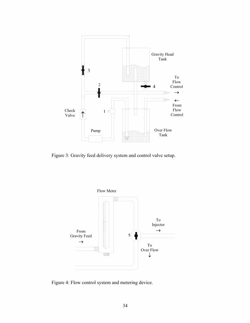
3.1.1 Gravity Feed System
The salt-water delivery system used for the current study is detailed in Figures 3 and 4.
The delivery system consists of an upper chamber, in which the gravity head is
maintained constant, and a lower chamber that serves as an overflow compartment. The
chambers are made from plastic cylindrical containers, black painted to reduce photo
aging of the Rhodamine dye associated with ambient light exposure. A single in-line
pump and a series of PVC pipes connecting the two containers allows the solution to be
circulated within the delivery system. The inline pump maintains a constant water level in
the upper container thus maintaining the proper gravity head and assures that the salt,
water, and Rhodamine dye are in a well-mixed state.
Several PVC valves are used to regulate the direction of the flow for the gravity feed
delivery system. For the pump to function properly, the excess air upstream of the pump
is removed by attaching a siphoning devise to the release valve (1). Prior to testing the
pump is used to increase the circulation through the delivery lines by opening valve (2).
Valve (3) is used to regulate the pumps flow from the overflow tank to the gravity head
33
Gravity Head Tank
Check Valve ↑
Figure 3: Gravity
FromGravity F
→
Figure 4: Flow co
3
ToFlow Control
Pum
feed
eed
ntrol
2
→ ←
From Flow
p
de
sy
1
livery system and control
r
ToOver
↓
stem and metering device
34
4
Control
Over Flow Tank
valve setup.
To Injector
→5Flow Mete
Flow
.

tank and is set in the open position during testing. Valve (4) is used to direct the mixed
saline solution from the gravity feed tank to the flow control system. The flow control
system is presented in Figure 4. Within the flow control system, an inline flow meter is
used to adjust and monitor the volumetric delivery rate. Beyond the flow meter a three-
way flow valve (5) is used to direct the saline solution to the injector or to the overflow
tank for recirculation.
3.1.2 Model Description
A 1/7th scale clear polycarbonate model of a room-corridor-room enclosure was
constructed for this study. A photograph of the room-corridor-room model is included as
Figure 5. The models dimensions are geometrically scaled to match those of the fire test
facility located at Combustion Science and Engineering, Inc. in Columbia, Maryland. The
design goals required the model to have walls that are optically transparent, an index of
refraction close to that of water, and strong / rigid construction, while also minimizing the
wall thickness and associated weight.
A variety of different plastics were analyzed and tested leading to the choice of 1/8th inch
clear polycarbonate. The particular scale was chosen so that the model could easily be
rotated within the large freshwater tank and lifted by a single person. The walls of the
model are joined with acrylic cement and the joints are sealed with clear silicone calk.
The walls are reinforced with 1-inch plastic braces in order to prevent separation and
increase rigidity. A series of cross members beneath the floor of the model were
implemented in the design for added structural stability.
35

Source Room (Note: injector not
shown)
Reinforcing Braces
Figure 5: Photograph of 1/7th scDashed lines are added to bette
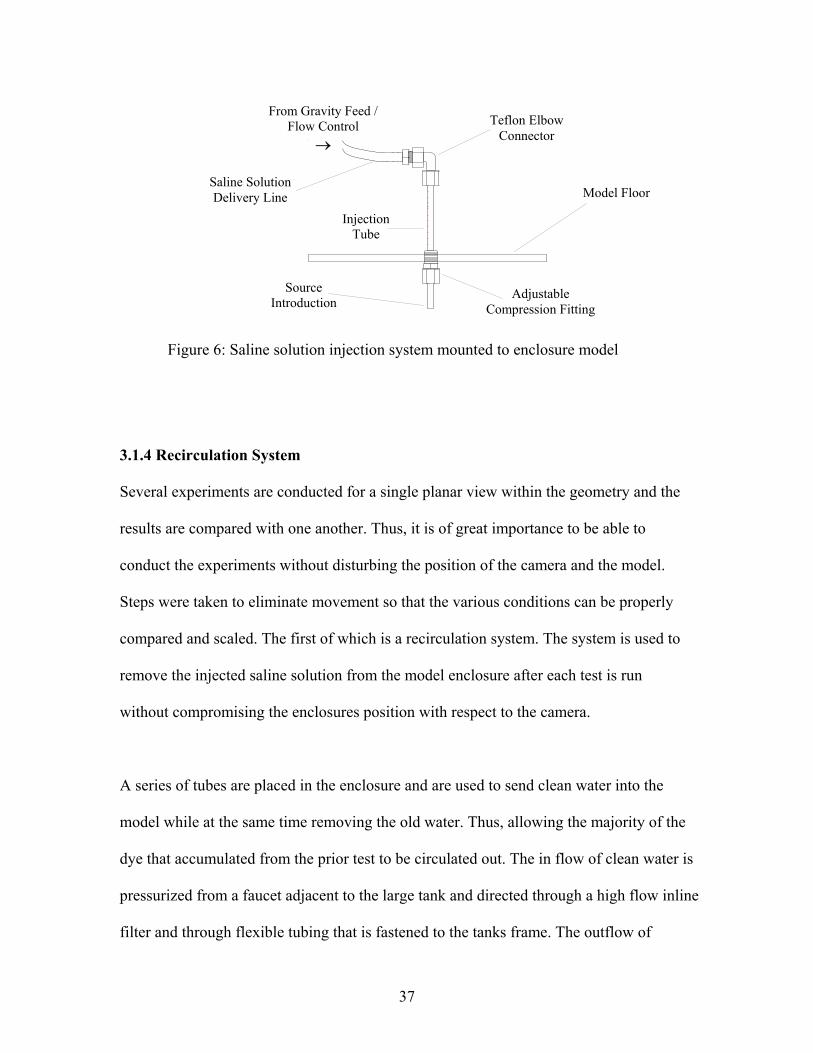
3.1.3 Injection System
The saline solution is introduced into t
system, which is depicted in Figure 6.
5.6 mm internal diameter, fitted with a
delivery line from the flow control. Th
adjustable Teflon compression fitting a
The compression fitting is mounted to
the model in the source room.
Corridor
Doorways
ale room-corridor-room enclosure mr illustrate boundary walls.
he model by means of an adjustable i
The system consists of a stainless ste
Teflon elbow connector attaching th
e stainless steel tube is set in place w
llowing easy vertical positioning of t
a 1/8th inch sheet of clear acrylic that
36
Adjacent Room
Model Ceiling
odel.
njection
el tube with a
e injector to a
ith an
he injector.
is attached to
From Gravity Feed / Flow Control
→ Teflon Elbow
Connector
Figure 6: Saline solution injection system mounted to enclosure
3.1.4 Recirculation System
Several experiments are conducted for a single planar view within the g
results are compared with one another. Thus, it is of great importance to
conduct the experiments without disturbing the position of the camera a
Steps were taken to eliminate movement so that the various conditions c
compared and scaled. The first of which is a recirculation system. The s
remove the injected saline solution from the model enclosure after each
without compromising the enclosures position with respect to the camer
A series of tubes are placed in the enclosure and are used to send clean
model while at the same time removing the old water. Thus, allowing th
dye that accumulated from the prior test to be circulated out. The in flow
pressurized from a faucet adjacent to the large tank and directed through
filter and through flexible tubing that is fastened to the tanks frame. The
Adjustable Compression FittIn n
Saline Solution Delivery Line r
37
Model Floo
ing
Source troductioInjection Tube
model
eometry and the
be able to
nd the model.
an be properly
ystem is used to
test is run
a.
water into the
e majority of the
of clean water is
a high flow inline
outflow of

“dirty” water is gravity driven; the flow rate is controlled by an adjustable PVC valve and
directed into a sink adjacent to the large tank. It is important to note that the water level
within the enclosure must remain slightly above that of the surrounding water in the large
tank to prevent the model from floating. Thus, the outflow valve must be monitored and
adjusted accordingly to maintain a constant water level. The water within the enclosure is
circulated until the presence of fluorescent dye is no longer visible.
3.1.5 Positioning System A positioning system illustrated in Figure 7 has been implemented in the experimental
setup in order to further restrict the movement of the model enclosure between
experiments. The entire system is constructed of Bosh aluminum framing. The model
rests on a stand fixed with two triangular aluminum plates that serve to stabilize the
enclosure and prevent any shifting with respect to the stand. The stand is connected to a
cross member that is mounted to the top of the large tank. The cross member is used for
positioning and to stabilize the frame itself. Additional support and weight is added to the
frame by means of cinder block stands located beneath the model. Cinder blocks are
placed on the cinder block stands after the positioning of the frame is set.
3.1.6 Optics
A 500-mW Argon Ion CW laser and a series of laser optics, illustrated in Figure 8, is
used to create the planar light sheet for the PLIF diagnostics. The laser is mounted to a
stand built with Bosh aluminum framing and the entire system is bolted to an optics table.
The initial beam is passed through a spatial filter and collimated with a dual convex lens.
38
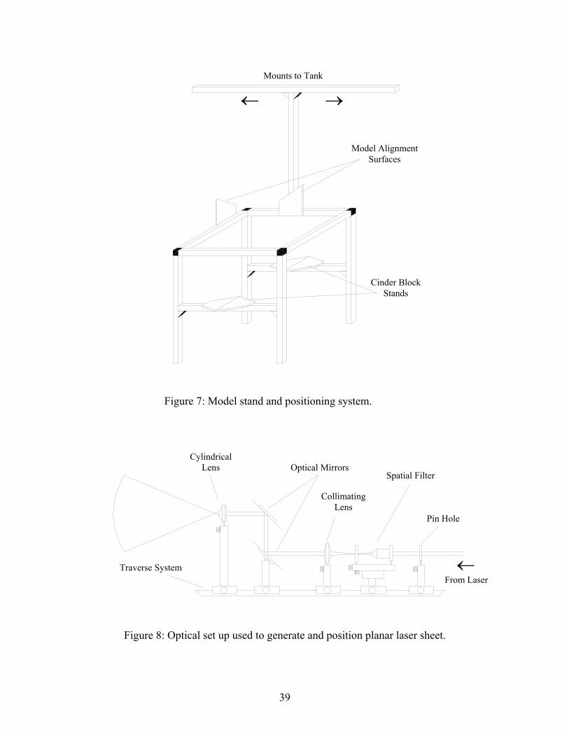
Figure 7: Model stand and position
Cylindrical
Lens Optical
Traverse System
Figure 8: Optical set up used to generate and
39
→
← Mounts to TankModel Alignment Surfaces
Cinder Block Stands
ing system.
Mirrors Spatial Filter
Collimating Lens
e
position planar laser s
Pin Hol
Fr
heet.
← om Laser

The spatial filter is used to produce a “clean” light sheet. The PLIF technique requires a
light sheet with a well-defined intensity profile. The argon-ion laser produces a Gaussian
light intensity profile. However, imperfections in optics result in spatial deviations from
this profile as shown in Figure 9. A spatial filter is used to remove imperfections in the
beam intensity profile. The spatial filter is composed of a microscopic objective and a
high intensity pinhole, both of which are aligned using a micro-traverse system. The
microscopic objective focuses the beam down to a point, in which it is passed through the
pinhole to remove spatial noise.
After the spatial filter and collimating lens, the beam is then redirected by a series of
optical mirrors. Finally, the collimated beam is passed through a cylindrical lens that
refocuses the light into a vertical planar sheet. The position of the cylindrical lens is
adjusted based on the spatial requirements of the light sheet.
Figure 9: Optical description of spatial filter and beam profile
40
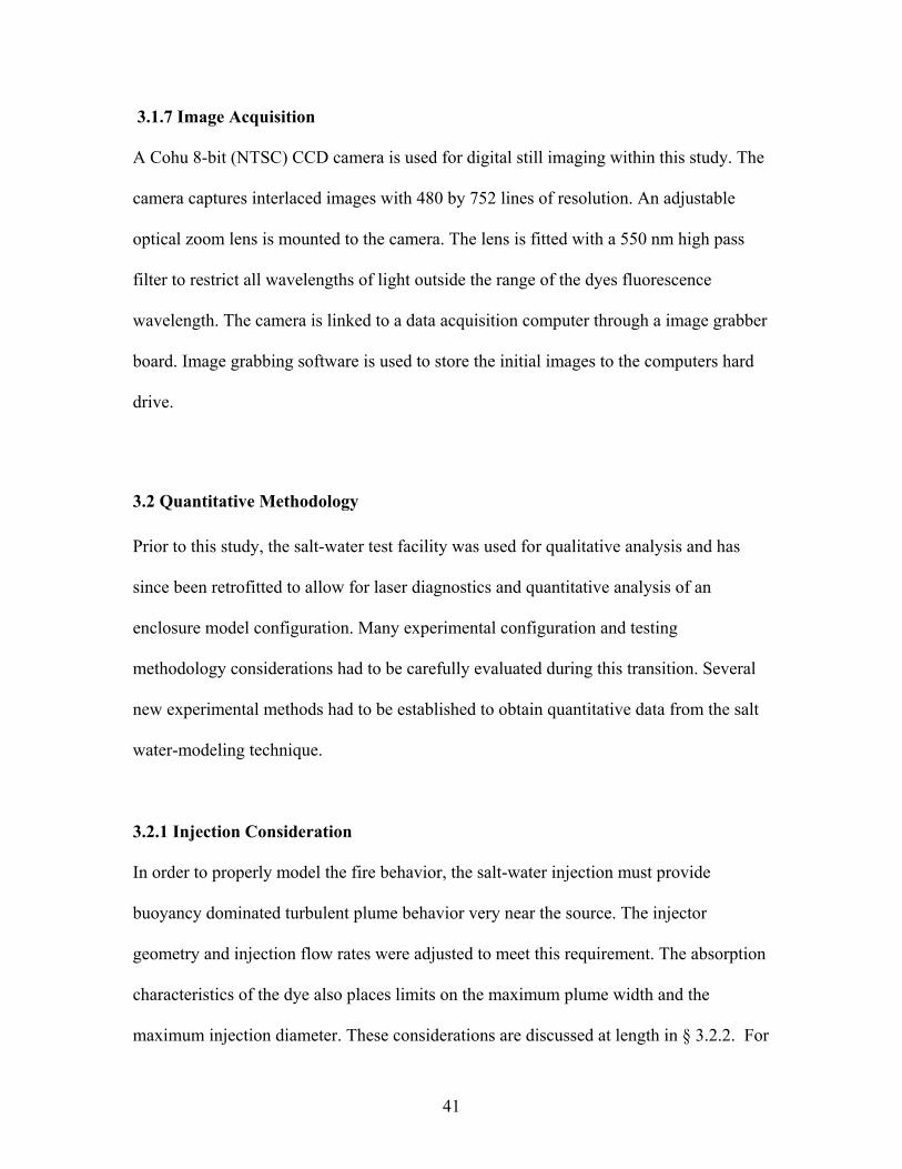
3.1.7 Image Acquisition A Cohu 8-bit (NTSC) CCD camera is used for digital still imaging within this study. The
camera captures interlaced images with 480 by 752 lines of resolution. An adjustable
optical zoom lens is mounted to the camera. The lens is fitted with a 550 nm high pass
filter to restrict all wavelengths of light outside the range of the dyes fluorescence
wavelength. The camera is linked to a data acquisition computer through a image grabber
board. Image grabbing software is used to store the initial images to the computers hard
drive.
3.2 Quantitative Methodology
Prior to this study, the salt-water test facility was used for qualitative analysis and has
since been retrofitted to allow for laser diagnostics and quantitative analysis of an
enclosure model configuration. Many experimental configuration and testing
methodology considerations had to be carefully evaluated during this transition. Several
new experimental methods had to be established to obtain quantitative data from the salt
water-modeling technique.
3.2.1 Injection Consideration
In order to properly model the fire behavior, the salt-water injection must provide
buoyancy dominated turbulent plume behavior very near the source. The injector
geometry and injection flow rates were adjusted to meet this requirement. The absorption
characteristics of the dye also places limits on the maximum plume width and the
maximum injection diameter. These considerations are discussed at length in § 3.2.2. For
41

the current study flow rates of 50, 100, 150 and 200 ml/min. were delivered to a 5.6 mm
diameter injector. These injector conditions provide analogous behavior and were within
the limits of our experimental constants.
The salt-water source is initially momentum dominated because the saline solution is
introduced as a jet. The initial jet-like behavior of the salt-water source differs from the
immediate buoyancy dominated behavior near the source in an accidental fire. The initial
momentum of the salt-water jet must be minimized to maintain analogous behavior
between the salt-water and fire flows. The initial velocity disturbs the validity of the salt-
water analogue close to the source. The initial momentum of the salt-water plume is
unimportant at a distance far from the source in which buoyancy dominates the flow
dynamics.19 This distance is characterized by the Morton length scale
( )2/1
24/1
4
−
=
oinj
injoM
gd
udl
ρρ
ρπ
where d is the diameter of the source, g is acceleration due to gravity, lM is the Morton
length scale and u is the injection velocity. For the current study, the Morton length
scale is used to determine the flow conditions necessary to produce a buoyancy
dominated plume. The momentum effects are considered insignificant and the plume
becomes buoyancy dominated at a distance above the source equal to L
inj
plume or .
Morton length scales and buoyancy dominated flow criterion are presented in Table 1 for
the experimental flow conditions. It should be noted that plume like behavior is achieved
within 20% of the enclosure height for all flow conditions.
Ml×5
42

, which should be very near the source. Previous
investigators determined that turbulent transition occurs when .
Table 1: Morton length scale results for salt-water model inlet conditions; (Ysalt = 0.10)
Flow Rate (ml/min)
l m
(mm)L plume
(mm)% of Model
Height
50.0 2.8 13.8 4.5
100.0 5.5 27.5 9.0
150.0 8.3 41.3 13.5
200.0 11.0 55.0 18.1
The salt-water flow is only analogous to the fire flow in the turbulent regime. It is
therefore essential for turbulent conditions to be established early in the flow field, i.e.
near the source. A critical Reynolds number criterion for turbulence dominated flow
based on the compartment height and the buoyancy induced convective velocity scale has
been specified by other investigators.8,16 The current investigation requires that turbulent
transition occurs close to the source.
A source based Grasholf number, provided in Eqn. (45), is calculated using the plume
dominated length scale, Lplume
35 In
this investigation, the flow is assumed to be turbulence dominated when
based on the plume dominated length scale L7105.1 ×>swsourceGr plume. Criteria for
turbulence-dominated flow based on critical Reynolds and Grasholf numbers are
provided in Table 2.
43
7105.1 ×>swsourceGr

Table 2: Important dimensionless turbulence criterion; (Ysalt = 0.10)
Flow Rate (ml/min) Re
50.0
100.0
150.0
200.0
swsourceGr
For the flows examined in this study, the
exception of 50 ml/min. Preliminary resul
scaling for this flow (50 ml/min.). Theref
presented in this investigation. However,
critical Reynolds number requirement spe
turbulent transition arguments, which are
this investigation, the critical Reynolds nu
may be overly conservative.35
3.2.2 PLIF Requirements
In order to obtain quantitative data within
that the requirements of the technique be
important characteristic of all fluorescent
and the path length of the incident light. A
begins to self absorb the incident light alo
in this study are only representative of qu
1.3E+08 3.4E+03
1.0E+09 3.9E+03
3.4E+09 4.6E+03
8.1E+09 4.7E+03
critical Grasholf number is achieved with the
ts demonstrated a significant discrepancy in the
ore, this flow was not used in the final analysis
all of the flows examined fall short of the
cified by other investigators. Based on the
the basis of the critical Grasholf number used in
mber recommended by previous investigators
the spatial domain of interest it is necessary
strictly followed. Light absorption is an
dyes. It is a function of the dye concentration
t high dye concentrations the excited dye
ng the beam path length. The images recorded
antitative data within the spatial domain where
44

light absorption does not affect the linear response of the dye. A critical path length has
been established for each planar sheet based on the light absorption properties inherent
with Rhodamine 6G dye.
Chandrasekar and Walker demonstrate that for a fluorescent dye at any arbitrary
concentration, the absorption of light for a beam path z can be computed by
( ) ( ) ( )dzzIzCzdI ee ⋅⋅−= ε (51)
where is the excitation intensity, ε is the extinction coefficient, and C is the dye
concentration.
eI
35,37 Guilbault and Arcoumanis suggest that the linear response of the
fluorescent dye is only valid when less then 5% of the excited light is absorbed.38,39
Assuming the concentration is constant along the path length, neglecting the attenuation
along the receiving path and assuming that is known at a critical value for z. Then Eqn.
(51) can be solved for a critical path length
eI
∫∫ −=
bI
Ie
e
dzCdII 0
2
1
1 ε (52)
( ) ( ) ( )CC
IICb⋅−
=⋅−
=εε
95.0lnln 12 (53)
where is the maximum excitation intensity, is the excitation intensity with
absorption, and b is the critical beam path length occurring at 95% excited light
fluorescence. The critical path length in which the dye excitation maintains a linear
relationship with concentration is presented in Figure 10 as a function of the
concentration of dye. The linearity of the dye’s fluorescence allows quantitative
1I 2I
45

0
0.01
0.02
0.03
0.04
0.05
0 5 10 15 20 25 30
Dye
Con
cent
ratio
n (m
g/L)
Figure 10: Maximum incidefluorescent dye maintains li
measurements to be obtained; Eqn.
measurements are valid.
The concentration of Rhodamine 6G
absorption properties of the dye. An
planar view, to produce the highest
linearity regime for the fluorescent
It has also been observed by previo
fluorescent dye used in this study (R
decay in the dye concentration. Add
solution based on the Davidson’s re
Critical Length, b (cm)
nt path length for which Rhodamine 6G near emission characteristics.(53) is used to control the spatial domain in which the
dye used in this study was chosen based on the light
optimum dye concentration was computed for each
light emission signal possible while staying within the
dye.
us researchers that residual chlorine reacts with the
hodamine 6G). The reaction causes a significant
itives and filtration are used to treat the dyed saline
commendations.40
46

3.2.3 Optimizing Image Quality
The limitations of the fluorescent dye restrict the use of high dye concentrations, so it is
necessary to adjust the camera settings to improve the image depth. The depth of the
captured image is descriptive of the amplitude between the minimum and maximum gray
level captured by the camera. A comparison of the minimum and maximum gain settings
on the camera is presented in Figure 11, which illustrates the light distribution within a
uniformly mixed volume; refer to § 3.2.4. As the image depth of the camera is increased
the magnitude of the fluctuations in the gray level increase as well. However, the
fluctuations are relatively the same with respect to the maximum gray level value.
Furthermore, when both intensity profiles are normalized by the maximum gray level
value, they are virtually identical as seen in Figure 12. Therefore, increasing the gain
increases the depth of the image without affecting the shape of the normalized signal.
By increasing the gain on the CCD camera, the amount of digital noise (salt & pepper)
within the image is also increased; however the signal to noise ratio remains nearly the
same. The signal to noise ratio is of great importance when performing any type of data
imaging. To reduce the amount of digital noise, multiple images are taken over a given
short time interval for transient experiments. Existing literature on PLIF techniques
supports the use of time-averaging images to reduce noise levels without reducing the
overall mean intensity level of the image. An optimization of the time-averaging period
(~1 second, 30 images) has been previously examined for similar flow conditions found
in gravity currents. For the current study this technique was employed and an optimal
47
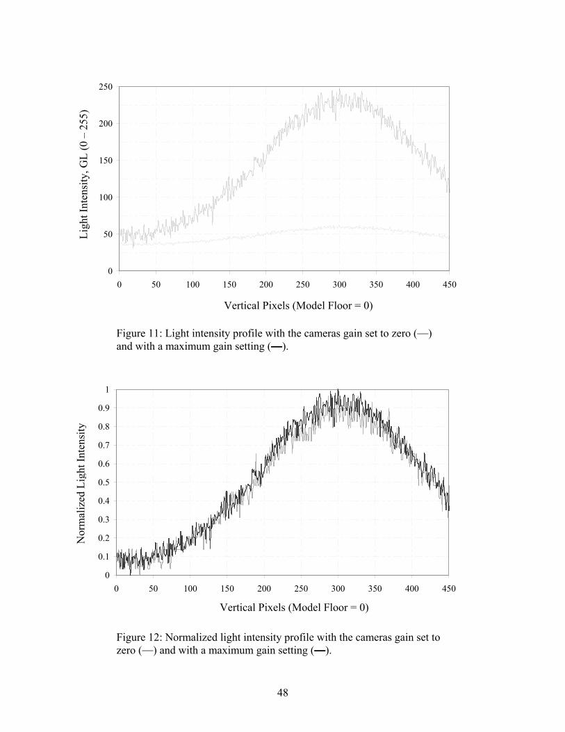
0
50
100
150
200
250
0 50 100 150 200 250 300 350 400 450
Ligh
t Int
ensi
ty, G
L (0
– 2
55)
Vertical Pixels (Model Floor = 0)
Figure 11: Light intensity profile with the cameras gain set to zero (˙) and with a maximum gain setting (˙).
0
0.1
0.2
0.3
0.4
0.5
0.6
0.7
0.8
0.9
1
0 50 100 150 200 250 300 350 400 450
Nor
mal
ized
Lig
ht In
tens
ity
Vertical Pixels (Model Floor = 0)
Figure 12: Normalized light intensity profile with the cameras gain set to zero (˙) and with a maximum gain setting (˙).
48
time-averaging period was obtained and applied to all images (~1/15 second, 4 images).
It is important to note that the flows evaluated in this work are slow moving relative to
the speed of the data acquisition systems buffer memory and that the digital noise
associated with the gain of the CCD camera is random. With this in mind the consecutive
images are viewed as a single time step. Averaging the consecutive images reduces the
random digital noise while the intensity of the signal remains unchanged. Preliminary
testing has been conducted to demonstrate that the flows are “frozen” within the sampling
period used in this study. A macro was written within the image acquisition software to
take two consecutive interlaced images that are 1/15th of a second apart and store them in
the buffer memory of the computer. The images are saved to the hard disk and the
procedure is repeated for each time step.
The images captured by the CCD camera are interlaced images with a resolution of 480
by 752 pixels. NTSC and PAL video images (US and European standards) are made up
of two (2) interlaced fields. The horizontal lines of the image are broken into odd and
even fields. Each field is captured over a period of 1/60th of a second resulting in a total
image exposure time of 1/30th of a second. As described previously, the slow moving
flows examined with in this study are considered frozen within this exposure time. An
international data language (IDL) program is written to separate the odd and even fields
of the interlaced image. The 240 odd and 240 even fields are stretched to represent two
images each with 480 horizontal lines. Finally, an average is taken of the odd and even
images. Incorporating this procedure with the time-averaging technique allows a single
49

time step to be represented by an average of four digital images. Thus, greatly increasing
the images signal to noise ratio.
Sources of error are presented by the digital noise linked with the cameras gain as well as
the background noise associated with the laser sheet interacting with the enclosure walls.
The background noise can be greatly reduced by taking a series of background images
prior to each experiment. After the experimental setup is complete, a series of 300
instantaneous images are taken with the laser sheet illuminating the selected slice within
the room. The laser sheet reflects off of surfaces to create background noise. The CCD
cameras high pass filter removes most of the noise, however the silicone caulk and the
enclosures walls have trace amounts of dye present and the sheet illuminates the
boundaries at the same wavelength as the fluoresced dye. The subtle noise associated
with the boundaries is quantitatively measured by averaging these images. This average
background image is subtracted from the instantaneous experimental images in post-
processing.
3.2.4 Light Sheet Distribution
Because of the Gaussian light intensity distribution, the vertical location of the light sheet
is of great significance. It is important that the sheet is introduced in such a manner that
the area of most interest is adequately illuminated, while at the same time providing
adequate illumination through out the entire domain of interest. Preliminary tests have
been conducted to locate the optimal light sheet dimensions and position, for each plane
of interest with in the room-corridor-room model.
50

While using PLIF diagnostics it is important to understand that the light emitted by the
excited dye is a function of the concentration of the dye and the intensity of the incident
laser light, refer to Eqn. (51). Since the light sheet produced from the Argon/Ion laser has
a Gaussian intensity profile, the experimental images not only describe the concentration
distribution of the dye but also the incident light intensity distribution. Only the dye / salt
dispersion is of interest so the effect of the light sheet distribution must be removed.
Previous studies provide details regarding calibration techniques for a non-uniform light
distribution.13 Calibration images are taken as a quantitative measurement of the light
intensity distribution within the enclosure and are used in post-processing to correct the
experimental images. For each test setup an average calibration image is needed due to
the geometric differences within the enclosure and the variances associated with
adjusting the corresponding light sheet. Calibration images are taken following a series of
experiments, with the model location unchanged. The model is filled with a known dye
concentration (0.01 mg/L), the laser sheet is activated, and a series of 300 instantaneous
images are taken and used to create a single average calibration image. The averaged
image represents the light sheet distribution within the spatial domain of the enclosure
and is used in converting the captured light intensity to a salt mass fraction.
3.2.5 Converting Light Intensity Measurements to Salt Mass Fraction, Y salt
Testing in this study and elsewhere has demonstrated that the relationship between the
fluoresced light intensity is purely a function of the dye concentration.37,38,40 This
relationship can be described by
51

[ ]DYECI 1= (54)
where I is the normalized light intensity (gray level) recorded by the camera, C1 is a
factor that includes the salt mass fraction, and [DYE] is the dye mass concentration. The
constant C1 is determined by a series of calibration images with known concentrations of
dye. The normalized intensity is measured for these images and the constant C1 is
determined from a linear curve fit of normalized intensity as a function of dye
concentration. Assuming that the concentration of dye and salt dilute similarly (as
discussed in § 1.1), the dye concentration [DYE] is related to the slat concentration
[SALT] by
[ ] [ ]SALTCDYE 2= (55)
C2 is determined by the initial salt and dye concentrations at injection. The salt mass
concentration can be expressed in terms of the salt mass fraction as follows:
[ ] swsaltsw
sw
sw
salt YVm
SALT ρρρ
== . (56)
Furthermore, an expression for the salt-water density in terms of the salt mass fraction
can be determined empirically. The density is given by
saltsw YCC 43 +=ρ , (57)
where C3 is the density of fresh water ( = 1000 kg/m3) and C4 is the constant relating the
salt mass fraction within a salt-water solution to the solutions density ( = 760 kg/m3).
Combining Eqns. (54) and (55)
[ ]SALTCCI 21= . (58)
Combining equations (56) and (58)
52
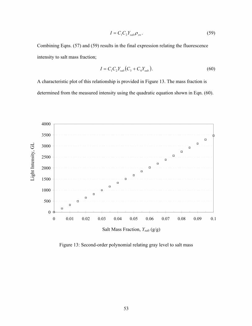
swsaltYCCI ρ21= . (59)
Combining Eqns. (57) and (59) results in the final expression relating the fluorescence
intensity to salt mass fraction;
( )saltsalt YCCYCCI 4321 += . (60)
A characteristic plot of this relationship is provided in Figure 13. The mass fraction is
determined from the measured intensity using the quadratic equation shown in Eqn. (60).
0
500
1000
1500
2000
2500
3000
3500
4000
0 0.01 0.02 0.03 0.04 0.05 0.06 0.07 0.08 0.09 0.1
Ligh
t Int
ensi
ty, G
L
Figure 13: Second-or
Salt Mass Fraction, Ysalt (g/g)
der polynomial relating gray level to salt mass
53

3.3 Experimental Procedure
The experimental procedure within this study follows a detailed methodology in order to
produce dependable and precise measurements. A checklist has been created to ensure
consistency, adequate documentation of the experiments and recording necessary
measurements. The checklist is provided in Appendix A. For each planar view the
positioning system, optics and the relative locations of the frame and injector are tested
and recorded. Along with the spatial considerations of the experimental setup, several
other important parameters are recorded using the checklist with regard to the diagnostics
and other experimental variables. Detailed descriptions of the experimental procedure
used for this study are included in Appendix B.
54

Chapter 4. Analysis
4.1 Calculating Dimensionless Parameters for Fire Test Data
The salt-water analogue requires the fire experimental results to be presented in terms of
dimensionless variables describing the dispersion within the enclosure. These variables
are computed from experimental data obtained from the full-scale fire experiment. The
following section provides an overview of the important variables and parameters for the
fire experiment and the basic computations of each dimensionless quantity. For a detailed
description of the derivation and scaling of governing equations for the full-scale fire
refer to Chapter 2. The scaled parameters from the fire experiment are used to convert the
local measurements at each of the five detectors in the room-corridor-room experiment
into dimensionless quantities that describe the dispersion dynamics. The local gas
temperatures shown in Figure 14 were converted into a dimensionless thermal dispersion
signature as shown in Figure 15 for comparison with the salt-water results. The local
smoke mass fraction measurements for the five detectors shown in Figure 16 were
converted to the dimensionless smoke dispersion signatures as shown in Figure 17 for an
analogous comparison with the salt-water results. The smoke and the thermal dispersion
signatures are plotted against the dimensionless time for the same conditions in the
previous smoke mass fraction and temperature time trace. A detailed examination of the
dispersion signatures for the fire and salt-water experiments is presented in Chapter 5.
Through this comparison the salt-water experiments are used to model the conditions of
interest within the full-scale fire experiment. The computations necessary for this
evaluation are described within this chapter for both the full-scale fire and salt-water
model experimental results.
55

0 25 50 75 100 12520
30
40
50
60
70
80
90
100
110
Gas
Tem
pera
ture
, Tfir
e (°C
)
Figure 14: Local Tfire at d RM1 – C, RM1 - S,
0 50
5
10
15
20
25
30
35
Ther
mal
Dis
pers
ion
Sign
atur
e, θ
T*
Dime
Figure 15: Local at de RM1 – C, RM1 - S,
*Tθ
Time (sec.)
etector for full-scale fire experiment: COR – C, COR - S, RM2 - C
10 15 20 t* nsionless Time, t*
tector for full-scale fire experiment: COR – C, COR - S, RM2 – C
56
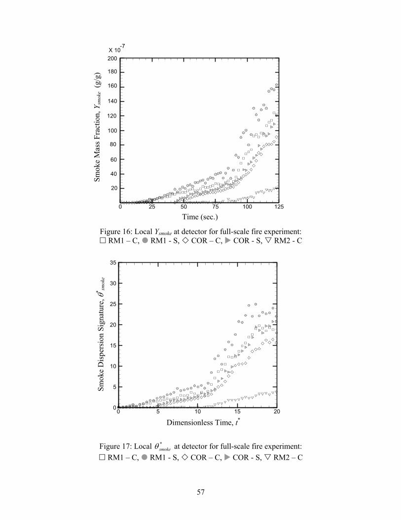
0 25 50 75 100 125
Smok
e M
ass F
ract
ion,
Ysm
oke
(g/g
)
Figure 16: Local Ysmoke at RM1 – C, RM1 - S,
0 50
5
10
15
20
25
30
35
Smok
e D
ispe
rsio
n Si
gnat
ure,
θ* sm
oke
Dim
Figure 17: Local at RM1 – C, RM1 - S,
*smokeθ
20
120
100
80
60
40
200
180
160
140
X 10-7
Time (sec.)
detector for full-scale fire experiment: COR – C, COR - S, RM2 - C
10 15 20
ensionless Time, t*
detector for full-scale fire experiment: COR – C, COR - S, RM2 – C
57

4.1.1 Dimensionless Energy Release Rate, *Q
The scaling performed in § 2.1.2 presents the density deficit of the thermal plume in
terms of a non-dimensional heat source strength term . This dimensionless parameter
describing the source strength takes the form
*Q
= 2/52/1
*
fopo LgTcQQ
ρ,
where ρo is the density of air, cp is the specific heat capacity of air, To is the ambient air
temperature, Lf is the enclosure height and Q is the energy release rate of the fire.
The energy release rate, , for the full-scale fire test data is calculated based on the fuel
type, geometry, and measured mass loss rate in which
Q
cf HAmQ ∆⋅⋅′′⋅= &χ
where χ is the combustion efficiency factor (< 1.0), m ′′& is the mass loss rate of the fuel
per unit area, Af is the fuel surface area, and cH∆ is the heat of combustion.2 Literature
values were chosen for the χ factor and the cH∆ for the respective fuel mixture, (75%
heptane and 25% toluene). A load cell was used to monitor the mass of fuel within the
full-scale experiment. A constant mass loss rate,
ffuel Amm ⋅′′= &&
was computed based on a linear fit of the load cell data for the burning duration of the
fuel.
58

4.1.2 Dimensionless Fire Time, *firet
The non-dimensional time for the full-scale fire experiment is derived in § 2.2.1 and
presented in terms of the source strength in which
( ) ( ) 2/13/1*
*
/ gLQ
tt
f
firefire −=
where t is the experimental (real) time and t is the dimensionless time for the full-
scale fire. The dimensionless time can be computed for any experimental time given a
dimensionless fire source strength, , and an enclosure height, L
fire*fire
*Q f .
4.1.3 Dimensionless Thermal Dispersion Signature, *Tθ
The buoyancy force that moves smoke in a fire is due to a density deficit resulting from a
temperature difference between the hot gasses and the cool ambient surroundings. A non-
dimensional thermal dispersion term, , can be used to describe this important
parameter as previously defined in Eqn (31):
*Tθ
( )( ) 3/2*
*
Q
TT oTT
−=β
θ
where oTT
1=β ,
where T is the buoyant gas temperature and To is the ambient air temperature. The local
gas temperatures at each detector are thus converted into thermal dispersion signatures
based on the dimensionless source strength.
59

4.1.4 Converting Optical Measurements to Smoke Mass Fraction, Y smoke
The full-scale fire experiment monitored the light obscuration at the local position of
each of the five detectors. A laser beam and photodiode assembly were mounted 5 cm in
front of each detector, to monitor the obscuration prior to entrance. The optical density of
smoke is calculated based on the measured attenuation of the beam of light passing
through the smoke. If the initial light intensity of the beam is Io when there is no smoke
present, then the reduced intensity (I) is given by the Lambert-Beer Law:2
( )CLII o κ−= exp (61)
where C is the mass concentration of smoke particles, L is the optical path length of the
beam and κ is the extinction coefficient. The optical density, D, is then defined in terms
of natural logarithms given by:41
CLIIDo
κ=
−= log
This expression can be rearranged to represent the mass concentration of smoke in terms
of the extinction coefficient, the optical path length and light attenuation yielding
⋅
−=
oII
LC log1
κ
A baseline light intensity is measured and averaged over a two-minute interval prior to
each test and is used within the calculations as the respective Io for each detector location.
The path length of 18 inches (0.4572 m) is maintained for the optical set up at each
location. Literature supports the assumption that κ is nearly universal and remains
constant for post-flame smoke produced in over-ventilated fires. The constant value used
for the mass specific extinction coefficient for post-flame generated smoke is 8.7 m2/g
60

with a 95% confidence interval of 1.1 m2/g. The calculated value of the mass
concentration of smoke particles, C, can also be viewed as a smoke density, ρsmoke. The
smoke density is used to calculate the mass fraction of smoke given by
mix
smokesmokeY
ρρ
=
Where ρmix is the density of the smoke and air mixture. It is assumed that the amount of
air is much larger then the amount of smoke particles. Thus, ρmix is found using the
properties of air and the ideal gas law for the local gas temperature. The mass fraction of
smoke is also used to define a dispersion variable similar to and . *Tθ
*swθ
4.1.5 Dimensionless Smoke Dispersion Signature, *smokeθ
Dimensional analysis of the fundamental equations allows the mass fraction of smoke to
be presented in terms of a non-dimensional value (refer to Eqn. 40)
( ) ( )
∆
=
c
smokeop
smokesmoke
HyTc
Q
Y3/2*
*θ
where is a smoke dispersion parameter, Y*smokeθ smoke is the mass fraction of the smoke at a
specific location, and ysmoke is the smoke yield defined as the mass of smoke generated at
the source per unit mass of fuel consumed. The variable incorporates the driving
force of the fire in terms of a non-dimensional energy release rate, , as well as the fuel
specific smoke yield. Thus, the smoke dispersion parameter is sensitive to the source
strength and the fuel type.
*smokeθ
*Q
61

4.2 Calculating Dimensionless Parameters for Salt-Water Model
In an analogous representation of the dispersion dynamics, the salt-water mass fraction
measurements shown in Figure 18 are converted into a dimensionless salt dispersion
signature shown in Figure 19 for each respective detector location. Thus, allowing a
direct comparison to be made between the dispersion terms for both systems. A detailed
assessment of these terms is presented in Chapter 5. The scaled terms used in the
conversion are based on experimental variables. An overview of the calculations is
presented in this chapter.
0 50 100 150 200 250 300 350
Salt
Mas
s Fra
ctio
n, (g
/g)
)
Figure 18: Local Ysalt at detflow rate of 100 ml/min and
RM1 – C, RM1 - S,
325
275
225
175
125
75
25
X 10-5
Time, (sec.
ector for salt-water model run with a initial salt mass fraction of 0.10 g/g. COR – C, COR - S, RM2 – C
62

0 5 10 15 200
5
10
15
20
25
30
35
Salt
Dis
pers
ion
Sign
atur
e, θ
* sw
*
Figure 19: Local flow rate of 100 ml/m
RM1 – C, RM
*sθ
4.2.1 Dimensionless Salt Mass F
For a proper analysis of dispersiv
source based form as the fire data
model is previously defined in C
Similar to the fire equations the s
mass flux of salt at the injector g
Dimensionless Time, t
at detector for salt-water model run with a in and initial salt mass fraction of 0.10 g/g.
1 - S, COR – C, COR - S, RM2 – C
w
lux, *saltm&
e terms, the salt-water results are scaled in the same
. The non-dimensional source strength for the salt-water
hapter 2 as
2/52/1*
swo
sourceswsalt Lg
mm
ρβ &
& = .
alt-water source strength can be presented in terms of a
iven by
( ) VYm injsaltswsource&& ρ= ,
63

where V is the volumetric flow rate, (Y& salt)inj is the mass fraction of salt generated at the
source, and ρsw is the density of the saline solution given by
( )injsaltoosw Yρρρ 76.0+= ,
where ρo is the density of fresh water.
4.2.2 Dimensionless Salt-Water Model Time, *swt
The non-dimensional time for the salt-water model derived in § 2.2.2 is similar to that of
the full-scale fire experiment and is also presented in terms of the source strength in
which
( ) ( ) 2/13/1*
*
/ gLm
tt
swsw
swsw −=
&
where t is the experimental time and t is the dimensionless time for the salt-water
model. The dimensionless time can be computed for any experimental time given a
dimensionless injection source strength, m , and an enclosure height, L
sw*sw
& *sw sw .
4.2.3 Dimensionless Salt Dispersion Signature, *swθ
Just as the buoyancy force moves smoke in a fire due to a thermal density deficit, the
hydraulic analogue has a buoyant force due to the density deficit between the salt-water
solution and the ambient fresh water surroundings. A non-dimensional salt-water
dispersion term, , can be used to describe this important parameter as previously
defined in Eqn. (46):
*swθ
64
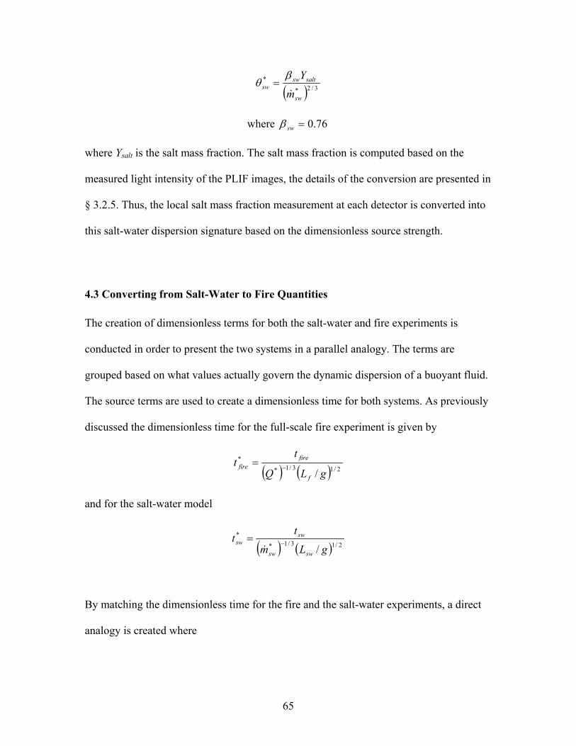
( ) 3/2*
*
sw
saltswsw
m
Y&
βθ =
where 0 76.=swβ
where Ysalt is the salt mass fraction. The salt mass fraction is computed based on the
measured light intensity of the PLIF images, the details of the conversion are presented in
§ 3.2.5. Thus, the local salt mass fraction measurement at each detector is converted into
this salt-water dispersion signature based on the dimensionless source strength.
4.3 Converting from Salt-Water to Fire Quantities
The creation of dimensionless terms for both the salt-water and fire experiments is
conducted in order to present the two systems in a parallel analogy. The terms are
grouped based on what values actually govern the dynamic dispersion of a buoyant fluid.
The source terms are used to create a dimensionless time for both systems. As previously
discussed the dimensionless time for the full-scale fire experiment is given by
( ) ( ) 2/13/1*
*
/ gLQ
tt
f
firefire −=
and for the salt-water model
( ) ( ) 2/13/1*
*
/ gLm
tt
swsw
swsw −=
&
By matching the dimensionless time for the fire and the salt-water experiments, a direct
analogy is created where
65

( ) ( ) ( ) ( ) 2/13/1*2/13/1* // gLm
t
gLQ
t
swsw
sw
f
fire−− =
&. (62)
The dimensionless time for the salt-water and fire systems is a direct function of the
dimensionless “source strength” and the length scale of the enclosure. Therefore,
simultaneously equating the dimensionless time provides a relationship in which the two
systems are in proper analogous form. Eqn. (61) is used to provide a salt-water model
time that corresponds to the full-scale fire time of interest. The salt-water model results
can be used to equate the fire conditions when the equality in Eqn. (61) is maintained.
Thus, the dispersion parameters are directly analogous,
, ***smokeTsw θθθ ≈≈
and the values of interest can be computed based on the experimental conditions of both
systems.
66

Chapter 5. Results and Discussion
5.1 Salt-Water Dispersion Analysis
The following section includes an assortment of sequential still images representing
several important stages of dispersion throughout the complex enclosure examined in the
current study. The dynamic flows are better understood through visualization;
nevertheless all images presented within this section are representative of quantitative
spatial and temporal measurements of the flow structure. The salt-water model images
are inverted vertically to provide a better comparison with the dispersion dynamics of hot
gasses within an enclosure. A scale consistent with the spatial domain is provided for all
images. The large tick marks correspond to a spacing of approximately 55 millimeters
and the small tick marks represent approximately 11 millimeters, in scale model space. In
the full-scale model, these dimensions correspond to 0.39 meters and 0.07 meters
respectively. The time scales for the Figures illustrated in this section, range from 2
seconds to 10 seconds in model space and 0.7 seconds to 3.8 seconds in full-scale space.
5.1.1 Initial Plume and Ceiling Jet
A vertical planar slice is taken within the source room of the enclosure model. As shown
in Figure 20, the planar sheet bisects the centerline of the injector and passes through the
doorway leading into the corridor. The primary stages of dispersion within the source
room of the salt-water model are captured in Figure 21. The large eddies seen in the
initial region of the plume demonstrate strong turbulent dispersion characteristics. The
turbulence is observed early on and is persistent throughout the height of the plume. The
dynamics of the plumes early interaction with the ceiling depicts the generation of large
67

tornoidal vortex structures. This initial vortex flow is bounded by the adjacent enclosure
wall and is forced to travel downward, quickly becoming engulfed by the plume. The
unobstructed vortex flow slowly travels away from the plumes centerline and is
dissipated by the underlying ceiling jet flow. The ceiling layer is inhomogeneous and has
a total thickness of approximately H/10 initially and grows to a height corresponding to
the doorsill (illustrated by a gray line in Figure 21).
(Enclosure Model)
Corridor
Inj
(Captured View)
Figure 20: Arial and side view of the planar sheet locSlice #1 bisects the injector and doorway of the sourc
68
SourceRoom
e
a
AdjacentRoom
Planar Slice
Doorway Sill
ctor
tion for slice #1. e room.

θ*
Figure 21: Series of primary images illustrating the plumes interaction with the ceiling. Images represent 2-second intervals in salt-water and 0.7-second intervals in fire experimental time, t* = 0.10.
69

5.1.2 Initial Doorway Flow Dynamics
The same planar view described by Figure 20 is examined as the time progresses and
filling occurs. The secondary stages of dispersion within the source room are shown in
Figure 22, where the ceiling layer descends below the doorsill and fluid spills into the
adjacent corridor. The initial ceiling jet impinges on the doorsill creating a reflected wave
directed toward the centerline of the plume. The wave creates a ceiling layer that is
approximately 60% thicker then the ceiling layer on the wall side. The transient stages in
the source room illustrate a non-homogeneous ceiling layer that descends to
approximately twice the height of the doorsill. As the ceiling layer spills into the adjacent
corridor the dynamics in the source room resemble steady state conditions. The
uniformity of the ceiling layer increases significantly and the interface between the
ceiling layer and the ambient environment becomes well established. Though the plume
penetrates the ceiling layer, the inhomogeneities near penetration mix out with increasing
radial distance from the plume centerline.
70

θ*
Figure 22: Series of images illustrating the source room ceiling layer doorway spill. Images represent 5-second intervals in salt-water and 1.9-second intervals in fire experimental time, t* = 0.27.
71

5.1.3 Corridor Frontal Flow Dynamics
A cross-section through the length of the corridor connecting the two compartments is
observed within this section as illustrated in Figure 23. The initial doorway flow seen in
Figure 24, spills from the source room into the corridor in a non-uniform and unsteady
manner. Once the spilling impinges the ceiling the flow experiences radial dispersion.
The walls adjacent to the doorway restrict the horizontal movement of the ceiling layer to
one direction. Small-scale wave reflection occurs throughout the corridor when the flow
impinges upon the enclosure walls. The magnitude of the reflected waves varies due to
the directional change of the original flow. Thus, creating cross currents and the
instabilities that are seen in the ceiling layer. The localized layer thickness and strength
increases temporally as the ceiling jet propagates along the length of the corridor. With
the leading ceiling jet thickness being approximately H/6 and the layer thickness above
the doorway being approximately H/3. When the ceiling jet reaches the far end of the
corridor a drastic reflected wave occurs that increases the total ceiling layer height to
roughly half the enclosure height, H/2.
(Enclosure Model) Injector
Corrido
(Captured V
Figure 23: Arial and side view of the
72
SourceRoom
AdjacentRoom
r
Planar Sliceiew)
planar sheet lo
Source RoomDoorway
Adjacent Room Doorway
cation for slice #3.

θ*
Figure 24: Series of images illustrating the corridor flow dynamics. Images represent 10-second intervals in salt-water and 3.8-second intervals in fire experimental time, t* = 0.54.
73

5.1.4 Secondary Doorway Flow Dynamics
The planar view examined in this section depicted by Figure 25. The final stage of
dispersion examined within this study, in which the corridor flow begins to spill into the
adjacent compartment is illustrated in Figure 26. The initial doorway flow from the
corridor into the adjacent room is much more stable then the doorway flow examined in §
5.1.2 and maintains very ordered characteristics. As the doorway flow impinges upon the
ceiling a very thin ceiling layer is created, with an initial thickness of less then H/15. The
ceiling layer is relatively homogeneous throughout the adjacent enclosure and does not
undergo any large scale mixing. The wave refection that occurs once the ceiling jet
reaches the far end of the enclosure does not create any significant mixing within the
ceiling layer. Beyond the final image of the series below no substantial dynamics are
observed as the adjacent room slowly fills with dispersed fluid. Only the initial spilling
and ceiling jet propagation is provided, as future images are redundant and unrelated
to the focus of this study.
(Enclosure Model)
Injector
(C
Figure 25: Arial and side view of
SourceRoom
r
AdjacentRoom
PlanarSliceaptured View
slice of pl
74
Corrido
)
anar she
DoorwaySill
AdjacentRoom
et location 4.
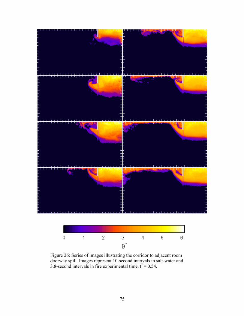
θ*
Figure 26: Series of images illustrating the corridor to adjacent room doorway spill. Images represent 10-second intervals in salt-water and 3.8-second intervals in fire experimental time, t* = 0.54.
75

5.2 Fire Response Time Analysis
The following section provides an evaluation of the experimental data obtained from the
full-scale fire test facility. The local conditions and dispersion dynamics are examined
within the enclosure at the relative position of each of the five ionization smoke
detectors. A schematic of the detector locations within the enclosure is provided by
Figure 27. The data is presented in a manner that tests the functionality of the detectors
response to various principles of dispersion. Please note, that any references made toward
a smoke detector is suggestive of only the ionization type units examined in this study.
Further examination is necessary to test this method for all smoke detection devices.
Corridor (COR)
COR - S
Figure 27: Arial view of the enclosure and s? represents the fire or salt-water source, ●smoke detectors and ■ represents sidewall m
76
Source Room(RM1)
Adjacent Room(RM2)
Source
RM1 - S
m r
RM1 - C
COR - C
RM2 - C
oke detector locations; epresents ceiling mounted ounted smoke detectors.
5.2.1 Local Conditions at the Time of Alarm
The local conditions including temperature and light obscuration, measured in the full-
scale test facility at the detector location, are examined to determine a possible threshold
for detector response. The threshold represents a dimensionless dispersion value that is
observed at any detector in the enclosure at the time of activation and allows the
activation time to be predicted using the model dispersion measurements. For each
detector the respective temperature rise and smoke mass fraction is computed from the
experimental data at the time of alarm. The localized values are presented in Figure 28
and Figure 29, for each respective location. The values were obtained in the full-scale fire
experiments by measuring the local gas temperatures with type-k thermocouples and the
local light obscuration with a laser and photodiode relative to each detectors position
within the enclosure. The computations composed in § 4.1.4 illustrate the conversion
from light obscuration to smoke mass fraction.
The temperature data suggests that the heat loss associated with the enclosure walls is
significant at the time of alarm. In comparing the localized gas temperatures for the
ceiling mounted detectors (RM1 - C, COR - C, RM2 - C), a trend is observed in which
the gas temperatures at alarm reduce considerably as the dispersion distance from the
source increases. While the initial front propagates from the source plume along the
ceiling, it experiences heat loss due to the temperature difference associated with the flow
and the enclosure walls. The transient exposure and subsequent losses are significant if
the front must travel great distances. The local gas temperatures for the sidewall-mounted
detectors (RM1 - S, COR - S) are subjected to even greater losses as gasses are
77
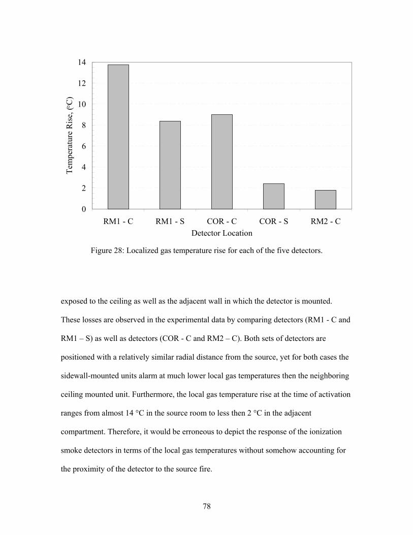
10
12
14, (
C)
e
T
R
p
s
c
r
c
s
t
°
0
2
4
6
8
RM1 - C RM1 - S COR - C COR - S RM2 - CDetector Location
Tem
pera
ture
Ris
e
Figure 28: Localized gas temperature rise for each of the five detectors.
xposed to the ceiling as well as the adjacent wall in which the detector is mounted.
hese losses are observed in the experimental data by comparing detectors (RM1 - C and
M1 – S) as well as detectors (COR - C and RM2 – C). Both sets of detectors are
ositioned with a relatively similar radial distance from the source, yet for both cases the
idewall-mounted units alarm at much lower local gas temperatures then the neighboring
eiling mounted unit. Furthermore, the local gas temperature rise at the time of activation
anges from almost 14 °C in the source room to less then 2 °C in the adjacent
ompartment. Therefore, it would be erroneous to depict the response of the ionization
moke detectors in terms of the local gas temperatures without somehow accounting for
he proximity of the detector to the source fire.
78
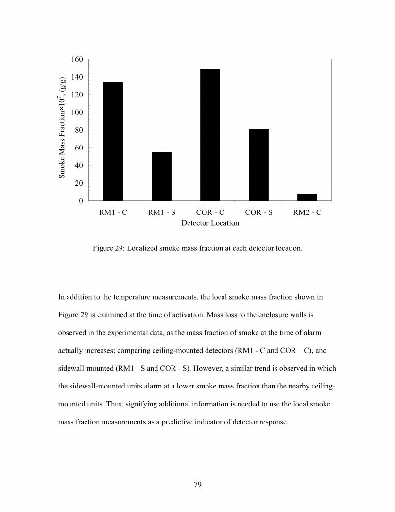
0
20
40
60
80
100
120
140
160
RM1 - C RM1 - S COR - C COR - S RM2 - CDetector Location
Smok
e M
ass F
ract
ion×
107 , (
g/g)
Figure 29: Localized smoke mass fraction at each detector location.
In addition to the temperature measurements, the local smoke mass fraction shown in
Figure 29 is examined at the time of activation. Mass loss to the enclosure walls is
observed in the experimental data, as the mass fraction of smoke at the time of alarm
actually increases; comparing ceiling-mounted detectors (RM1 - C and COR – C), and
sidewall-mounted (RM1 - S and COR - S). However, a similar trend is observed in which
the sidewall-mounted units alarm at a lower smoke mass fraction than the nearby ceiling-
mounted units. Thus, signifying additional information is needed to use the local smoke
mass fraction measurements as a predictive indicator of detector response.
79

5.2.2 Dispersion and Detector Response Times
The initial presence of dispersed gasses, presented in this discussion as the front arrival,
is an important element in characterizing the response of a smoke detector. As no visual
data was recorded for the full-scale fire tests, the time associated with the front arrival
was estimated from local measurements. The thermal front (based on the temperature
data) arrives at the same time if not earlier then any observed change in light obscuration
as shown in comparing Figure 14 with Figure 16 from § 4.1. As a result, the initial
occurrence of an increasing local gas temperature is used as an approximation for the
presence of the front for each respective location. The front arrival time represents the
time from which the fuel is first ignited to the estimated arrival of the smoke. In addition,
the time lag between the front arrival and the activation time of the detector is identified
as the activation delay time for this discussion. The front arrival times and delay response
times associated with each respective detector location are presented in Figure 30 and
Figure 31. It should be noted that the sum of the front arrival time and delay time
represents the detector activation time. A previous discussion in § 5.2.1 suggested that the
orientation of the smoke detector is a significant factor in determining its response.
Therefore, the following results are separated by orientation to better evaluate the
response properties. The front arrival and lag time of the ceiling-mounted units is shown
in Figure 30 and Figure 31 is representative of sidewall-mounted units.
The detector lag times maintain a relatively constant value and seem to be independent of
the detector location and relative position with respect to the source, as shown in Figure
30 and Figure 31. The sidewall-mounted detectors have a mean delay time of 13.5
80

0
10
20
30
40
50
60
70
80
RM1 - C COR - C RM2 - CDetector Location
Tim
e, (s
)
Figure 30: Ceiling-mounted ionization smoke detector response data from full-scale fire experiments; front arrival time, detector activation lag.
Note: detector activation time is the sum of the arrival and lag times.
0
10
20
30
40
50
60
70
80
RM1 - S COR - SDetector Location
Tim
e, (s
)
Figure 31 Sidewall-mounted ionization smoke detector response data from full-scale fire experiments; front arrival time, detector activation lag.
Note: detector activation time is the sum of the arrival and lag times.
81
seconds and a standard deviation of 5% and the ceiling-mounted detectors have a mean
delay time of 27.5 seconds and a standard deviation of 22%. The data suggests that the
orientation of the detector effects the lag time associated with its response. The difference
in response times may be due to the unit’s sensing chamber orientation with respect to the
flow or due to the increased flow velocities, which are not examined or discussed within
this study. However, existing literature does suggest the detector response lag is directly
related to the external flow velocity.34 Additionally, the front arrival time provides a first
order approximation for the detector response assuming the lag time remains relatively
constant. A discussion and comparison of the lag times for the full-scale and salt-water
model results is presented in § 5.3.2.
5.3 Predicting Detector Response Time
The following section provides a detailed comparison of the quantitative results obtained
from the salt-water experiments conducted within this study with the data acquired from
the full-scale test facility. The relevance of the experimental results with regards to
detector response is established in this discussion. A comparative analysis between fire
and salt-water model data is conducted with a focus on dimensionless front arrival times,
detector activation lag times and dimensionless dispersion parameters. A collection of
tables summarizing the important parameters and times described in this section is
included in Appendix A, for the fire and salt-water experiments.
82
5.3.1 Front Arrival Comparison
To facilitate the comparative analysis, the temporal results of the salt-water model and
full-scale fire experiments are dimensionless as discussed in Chapter 4. The arrival of the
front in the salt-water experiments was determined based on the initial fluorescence of
the dyed salt-water mixture for each location of interest. Both visual and quantitative data
were used to establish the front arrival times. The front arrival times for the geometrically
scaled detector locations are presented in terms of detector location and non-dimensional
time, t*. As illustrated in Figure 32, the front arrival times for dispersive flows in
the salt-water model are in excellent agreement with the full-scale fire test data. The
minor discrepancies in which the salt-water model “over predicts” the front arrival may
be due to experimental error in the full-scale experiment. There is a delay time associated
with the thermocouple measurements that would create a lag in the estimation of the front
arrival from the measured the local gas temperatures. This discrepancy may also be due
to the fact that the salt-water model cannot account for the reduction in buoyant forces
due to heat loss. 6,7,8,15 The results discussed in § 5.2.2 demonstrate that the front arrival
time provides a first order approximation of the detector response times. However, to
completely describe the detector response time, the lag time for the detector to alarm,
after the front has arrived, must also be considered. In fact, the lag time associated with
the detection devices examined in this study is often of the same order as the front arrival
time. This lag time is largely dependent on the interaction with the detector. Therefore, a
model for the lag time and appropriate measurements for the model inputs would be
required to accurately use salt-water modeling to predict smoke detector activation.
83
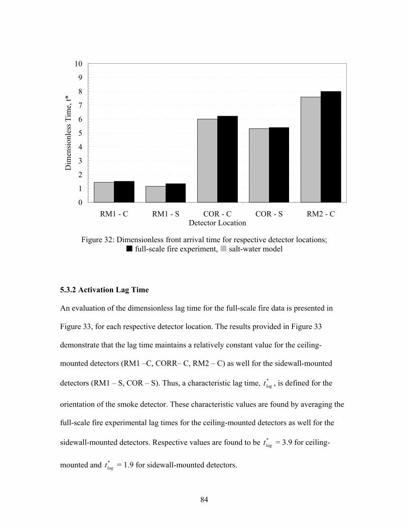
0
1
2
3
4
5
6
7
8
9
10
RM1 - C RM1 - S COR - C COR - S RM2 - CDetector Location
Dim
ensi
onle
ss T
ime,
t*
Figure 32: Dimensionless front arrival time for respective detector locations;
full-scale fire experiment, salt-water model
5.3.2 Activation Lag Time
An evaluation of the dimensionless lag time for the full-scale fire data is presented in
Figure 33, for each respective detector location. The results provided in Figure 33
demonstrate that the lag time maintains a relatively constant value for the ceiling-
mounted detectors (RM1 –C, CORR– C, RM2 – C) as well for the sidewall-mounted
detectors (RM1 – S, COR – S). Thus, a characteristic lag time, t , is defined for the
orientation of the smoke detector. These characteristic values are found by averaging the
full-scale fire experimental lag times for the ceiling-mounted detectors as well for the
sidewall-mounted detectors. Respective values are found to be t = 3.9 for ceiling-
mounted and t = 1.9 for sidewall-mounted detectors.
*lag
*lag
*lag
84

0
1
2
3
4
5
RM1 - C RM1 - S COR - C COR - S RM2 - CDetector Location
Dim
ensi
onle
ss T
ime,
t*
.
Figure 33: Dimensionless activation lag times for respective detector locations;
full-scale fire experiment
5.3.3 Detector Response Time Predictions By combining the salt-water model front arrival time described in § 5.3.1 with the
described in § 5.3.2, a simple model is created for predicting the activation times of each
smoke detector. The predicted activation times are compared to the actual response time
from the full-scale experiment in Figure 34. The model predicts the activation times at
every location within the enclosure with very good accuracy. The dimensionless
predictions are converted into actual time using the methodology described in § 4.3. The
model results are presented alongside the “real” experimental activation times from the
full-scale fire experiment within Table 3 including a calculation of the percent error
associated with the prediction. The average error in the response time prediction is less
*lagt
85

0
2
4
6
8
10
12
14
RM1 - C RM1 - S COR - C COR - S RM2 - CDetector Location
Dim
ensi
onle
ss T
ime,
t*
Figure 34: Salt-water models predicted smoke detector response times; salt-water model prediction, actual activation time
then 5% for four of the five detector locations examined within this study (RM1 –C, RM1
– S, CORR – C, COR – S). The response time prediction for the furthest detector from
the source (RM2 – C), located in the adjacent room, was still accurately modeled with an
error of around 13%. The increased error associated with detector RM2 – C, is most
likely due to the poor resolution seen in salt-water model results. At this location the
arrival of the dispersive front was difficult to ascertain and a detailed analysis of these
results is presented in § 5.4. The simple method used to model the smoke detector
activation times shows promise as a predictive tool and provides an excellent foundation
for future research pertaining to the objectives of this study. More advanced models may
include such things as velocity measurements and detector entrance lag correlations.
86

Table 3: Dimensionless and actual predicted detector response times
Detector Location Predicted Real Percent
Error Predicted Real Percent Error
RM1 - C 5.5 5.7 4 38 40.0 4
RM1 - S 3.4 3.2 6 23 22.0 6
COR - C 10.2 10.6 4 71 74.0 4
COR - S 7.4 7.2 3 52 50.0 3
RM2 - C 12.0 10.5 13 84 73.5 13
Actual Activation Times, (sec.)Dimensionless Activation Times, t*
5.4 Salt-Water and Fire Dispersive Parameter Comparison 5.4.1 Dispersion Comparison at Activation Time
Dimensionless signatures that characterize the dispersion for both the salt-water and full-
scale fire experiments are presented within this section at the time in which each detector
alarms. The dimensional analysis of the governing equations, presented in Chapter 2,
describes the importance of these dispersion parameters and the manner in which they are
computed is presented in Chapter 4. It should be noted that the salt-water analogue is
representative of the dispersive characteristics of an adiabatic fire with a constant source
strength. Thus, small discrepancies in terms of dispersion characteristics are expected due
to the non-ideal boundary conditions associated with a real fire. The thermal dispersion
parameter, , the smoke dispersion parameter, , and the salt-water dispersion
parameter, , are all computed at the time of activation for each respective detector
location and the results are illustrated in Figure 35. At the time of alarm, the relative
value of with respect to detector location is comparable to the for the full-scale
*Tθ
*swθ
*sw
*smokeθ
θ *Tθ
87
fire. However, the magnitude of at detector locations (RM1 –C, RM1 – S, CORR – C,
COR – S) is around three times greater then the . This may be due to the fact that the
salt-water model does not account for the reduction in gas temperatures associated with
heat loss to the enclosure walls. If the losses are significant the model will over predict
the temperature dependent . The comparison presented in Figure 35 suggests that the
heat losses are significant throughout the enclosure geometry. The discrepancy may also
be due to the response lag time associated with the type-k thermocouples used to measure
the local gas temperatures in the full-scale fire experiment. The amplified dispersion
values seen at locations RM1 –C, RM1 – S, CORR – C, COR – S is not observed at
location RM2 – C. The difference may be due to the fact that the resolution of the
experimental data at this location was poor due to the low levels of dyed saline solution
and erratic nature of the flow. A detailed evaluation of these results is presented in §
5.4.2.
*swθ
<
*Tθ
*Tθ
*θ
No significant trends are observed in comparing the salt-water models and the smoke
dispersion parameter, , for the full-scale fire experiment. However, a constant
value of is observed for the ceiling mounted units (RM1 – C, COR – C) and a
constant value of is observed for the sidewall mounted units (RM1 – S, COR –
S) at the time of detector activation. Once again, the ceiling mounted detector located in
the adjacent room (RM2 – C) does not follow the trends observed at the other locations
within the enclosure, with a . The lack of consistency at this location suggests
*swθ
*smokeθ
1≈
2* ≈smokeθ
θ *smoke
1.0smoke
88

0
2
4
6
8
10
12
14
16
18
20
RM1 - C RM1 - S COR - C COR - S RM2 - CDetector Location
Dim
ensi
onle
ss D
ispe
rsio
n Pa
ram
eter
,
θ*
Figure 35: Local dimensionless dispersion signature at detector activation; , , *
smokeθ *Tθ
*swθ
that the poor resolution and erratic nature of the flow presents a significant source of
error. Further examination of the temporal evolution of the scaled salt-water and fire data
at each detector location is essential for determining the reasons for this discrepancy.
5.4.2 Evolving Dispersion Signature Comparison
The temporal evolution of the salt-water and fire dimensionless dispersion signature is
presented in Figure 36 through Figure 40, for each detector location. A general
description of the trends observed throughout the enclosure is presented within this
section. Followed by an evaluation of the local salt-water and fire dispersion parameters
and the variations observed at each location within the enclosure.
89

This study has demonstrated that the scaled front arrival times for the fire and the salt-
water systems compare favorably. However, the experimental data suggests that the heat
losses down stream of the source significantly reduce the dispersion signature magnitudes
from the predicted values measured in the ‘adiabatic’ salt-water analogue. The heat loss
to the surroundings is a function of the temperature difference between the gasses and the
adjacent surfaces as well as the flow velocity, thus it is difficult to correct for. The losses
are very strong as the initial front arrives and become less significant as the boundaries
heat up as shown in Figure 36 through Figure 40.
A comparative analysis demonstrates that for all five of the detector locations the salt-
water dispersion signature, , increases at the same dimensionless time, t*, as the
smoke and thermal dispersion signatures, and , for the full-scale fire. Yet, the
fire dimensionless dispersion signature illustrates a slow increase in magnitude when
presented with the salt-water results that are nearly discontinuous at the front arrival. The
salt-water results throughout the enclosure suggest a strong initial front. At all locations
examined within this study is consistently smaller and tends to lag behind . This
trend may be due to experimental error in the full-scale obscuration measurements or
may be due to an assumption made in defining . The measurements taken in the full-
scale experiment demonstrate the erratic nature of a fire with an unsteady source in which
multiple variations in the temperature rise are observed for a single location and neither
the temperature nor the light obscuration measurements converge toward any steady state
value. The details associated with each location of interest within the enclosure are
presented in a manner that allows the reader to understand and visualize the comparison
*swθ
*smokeθ
*smokeθ
θ
*Tθ
*Tθ
*smoke
90

made between the full-scale and model results. The detector locations described in this
section are illustrated early on in § 5.2 in Figure 27.
Detector RM1-C is ceiling mounted in the source room and is located near the initial
plume impingement on the ceiling. The important dimensionless signatures that describe
dispersion for the salt-water and fire experiments are presented for this detector location
as a function of the subsequent dimensionless time in Figure 36. The salt-water
dispersion parameter, , at this location increases rapidly upon front arrival and begins
to plateau to a value ranging between 27 and 34. The fluctuations in may be due to
the observed turbulent conditions at this particular location. The small separation
(approximately ) observed with varying flow conditions suggests that the scaling
parameters are not entirely descriptive of the flow behavior. When the flow rates change
the virtual origin changes. Modifying the length scale by the virtual origin effect
improves the scaling. However, for consistency the length scale used in this study is
based on the enclosure height.
*swθ
*swθ
%10±
The thermal dispersion signature, , for RM1-C initially increases at the same
dimensionless time, t
*Tθ
*, as for the salt-water model, but at a much lower rate. A sharp
increase of is observed at t* ~ 10, where the slope of closely resembles the initial
portion of the salt-water model. The temporal evolution of reveals the unsteady nature
of the fire, a level of complexity that is not accounted for in the hydraulic analogue. This
secondary slope may be due to the ceiling layer in the source room contributing to the
*swθ
*Tθ
*Tθ
θ *T
91

0 5 10 15 200
5
10
15
20
25
30
35
40
45
Dim
ensi
onle
ss D
ispe
rsio
n Pa
ram
eter
, θ *
Dimensionless Time, t*
Figure 36: Dispersion parameters at detector location RM1 – C , , ( 200 ml/min, 150 ml/min, 100 ml/min) *
Tθ*smokeθ *
swθ
vaporization of the fuel or restricting the amount of air being entrained into the
combustion region. At this location, follows the same trends as described for
except with a reduction in slope and magnitude. It is important to note that and
maintain the same order of magnitude as , for the duration of the experiment.
*smokeθ
θ
*Tθ
*smokeθ*
Tθ
*sw
Similar observations are made when examining the dimensionless dispersion parameters
at RM1–S, mounted on the sidewall of the source room, as shown in Figure 37. However,
the scaling separation of is greatly improved between flow rates (approximately
) in comparison to the neighboring detector RM1–C. In addition, the fluctuations in
*swθ
%6±
92

0 5 10 15 200
5
10
15
20
25
30
35
40
45
Dim
ensi
onle
ss D
ispe
rsio
n Pa
ram
eter
, θ*
Dimensionless Time, t*
Figure 37: Evolution of dispersion parameters for detector RM1 – S , , ( 200 ml/min, 150 ml/min, 100 ml/min) *
Tθ*smokeθ *
swθ
*swθ
θ
are less significant than what is observed at RM1–C. The improvement in scaling
and stability is likely due to the detectors positioning being outside of the turbulent plume
/ ceiling jet interface. Again demonstrates a sharp initial increase, which begins to
level off as if it were going to converge to a constant value. The for this location has a
sharper initial and secondary slope compared to RM1 - C and achieves a maximum value
at . The value is almost identical to that of RM1-C, in which it lags behind
the and experiences the same secondary increase but at a lower magnitude.
Additionally, , and increase initially at approximately the same t*.
*swθ
*swθ
*Tθ
43* ≈T
*Tθ
*smokeθ
* *smokeθTθ
93

Detector COR-C is mounted on the ceiling of the corridor outside of the doorway leading
into the adjacent room, as pictured in Figure 27. A comparison of the dimensionless
dispersion parameters for COR–C is provided in Figure 38. At this location the salt-
water and fire dispersion parameters are significantly closer in magnitude for the duration
of the experiment. Again, the initial increases at the same t* as and with
the initial slope of being larger. Separation is observed in for the different flow
rates at t . For the salt-water model a more gradual mixing process is observed at
this location demonstrated by the slower increase in . This may be due to the subtle
*swθ *
Tθ*smokeθ
*swθ *
swθ
15* >
*swθ
0 5 10 15 200
5
10
15
20
25
Dim
ensi
onle
ss D
ispe
rsio
n Pa
ram
eter
, θ*
Dimensionless Time, t*
Figure 38: Evolution of dispersion parameters for detector COR – C , , ( 150 ml/min, 100 ml/min) *
Tθ*smokeθ *
swθ
94

spill process from the source room into the corridor such that the front is initially weak
and increases as it grows. The value is still lagging behind though the
magnitudes are closer than what is observed at RM1–C and RM1–S.
*smokeθ *
Tθ
Detector COR - S is sidewall mounted in the corridor outside of the doorway leading into
the adjacent room as illustrated in Figure 27. It should be noted that the manner and
duration of the salt-water experiments at this location differ from the other four detector
locations. The results shown in Figure 39 are representative of three tests, run at the same
flow conditions with an injection rate of 100 ml/min. This location was the first examined
in the current study in which the reproducibility of the technique was tested. Though, the
95

*0 5 10 15 200
1
2
3
4
5
6
7
Dim
ensi
onle
ss D
ispe
rsio
n Pa
ram
eter
, θ*
Dimensionless Time, t*
Figure 39: Evolution of dispersion parameters for detector COR – S , , @ 100 ml/min ( Test 1, Test 2) *
Tθ*smokeθ *
swθ
experiments were run for a shorter duration, the results encompass the conditions beyond
the time of detector activation and illustrate the initial flow dynamics, which satisfies the
intent of this study. The observations for COR - S are relatively the same as for COR – C,
however the slopes of the dispersive parameters are less similar.
Detector RM2 - C is ceiling mounted in the room adjacent to the source room. The exact
location of RM2 – C is provided in Figure 27. The initial arrival of the front for the salt-
water model is more difficult to distinguish at this location. The flow visualization
images in Figure 26, help describe what is seen in the dispersion data for the adjacent
room as illustrated in Figure 40. The subtle spilling from the corridor initially releases
96

0 5 10 15 200
2
4
6
8
10
12
14
Dim
ensi
onle
ss D
ispe
rsio
n Pa
ram
eter
, θ*
Dimensionless Time, t*
Figure 40: Evolution of dispersion parameters for detector RM2 – C , , ( 150 ml/min, 100 ml/min) *
Tθ*smokeθ *
swθ
small quantities of dispersed fluid into the adjacent room, which arrive at the detector
location at a variety of times. Therefore, once the doorway spill from the corridor
becomes steady, increases similar to . Although more scatter is observed in ,
the value of increases at the same rate and demonstrates similar erratic characteristics
early on as seen in the . Once again, the lags behind in magnitude and
maintains a relatively weak rate of rise.
*swθ *
Tθ*swθ
*Tθ
*swθ *
smokeθ *Tθ
97

Chapter 6. Conclusions
This study successfully used planar laser induced fluorescent (PLIF) diagnostics in
conjunction with the salt-water analogue to obtain quantitative non-intrusive
measurements of dispersion dynamics within a complex enclosure. The spatial and
temporal resolved images provide a detailed look into the flow structures and dispersive
dynamics for an ideal environment. The quantitative results of the PLIF technique
allowed for the time evolution of dispersion parameters from the salt-water model and the
full-scale fire to be compared with a detailed examination of the detector activation event.
The source based scaling used in this study proved effective in the comparative analysis
of the salt-water and fire experiments. The front arrival times measured for both the salt-
water and full-scale fire tests were made dimensionless and an excellent agreement was
observed between the two systems. The scaled salt-water data for various flow conditions
and salt mass fractions collapsed together internally with very good agreement. However,
the heat losses and unsteady nature of the full-scale fire present non-ideal boundary
conditions making comparisons of fire and salt-water analogue signatures challenging.
Nevertheless, these dispersion signatures stay within the same order of magnitude
throughout the duration of the tests and at every location examined within the enclosure
even without correcting for heat loss effects. Furthermore, the heat loss effects
demonstrate little significance with respect to convective dispersion dynamics within the
enclosure. In addition, the scaled smoke detector activation times were shown to be a
dynamic effect demonstrating little correlation with local obscuration or temperature.
98

This study reveals that although the magnitude of the local gas temperatures and smoke
concentrations impact the detector response, a simple model based on these values alone
cannot be used as a predictive indicator of detector response time. A more rational
modeling alterative has been introduced where the detector response time is modeled
based on the combination of a front arrival time and a detector lag time. The results show
that the salt-water model accurately predicts the front arrival time at all detector
locations. The activation lag time following the arrival of the front is of the same order
and its significance must be appreciated. This lag reduces substantially with an increased
flow velocity and is a strong function of the geometric configuration of the detectors
housing as well as the relative positioning within the enclosure, i.e. ceiling or sidewall
mounted. The results of the full-scale fire experiment demonstrate that the lag time
maintains a relatively constant value throughout the enclosure for the ionization type
smoke detectors examined in this study. However, the constant value for the lag time
does change based on whether the detector is ceiling mounted or sidewall mounted.
Based on these findings a constant value is used for the lag time and incorporated in the
simple predictive model. Using this methodology the salt-water model accurately predicts
the response time of the smoke detectors with very little error. A more sophisticated time
lag model may prove necessary as more fire data becomes available. Overall, the salt-
water modeling technique shows promise as a predictive tool in establishing the response
of ionization smoke detectors within a complex environment.
99
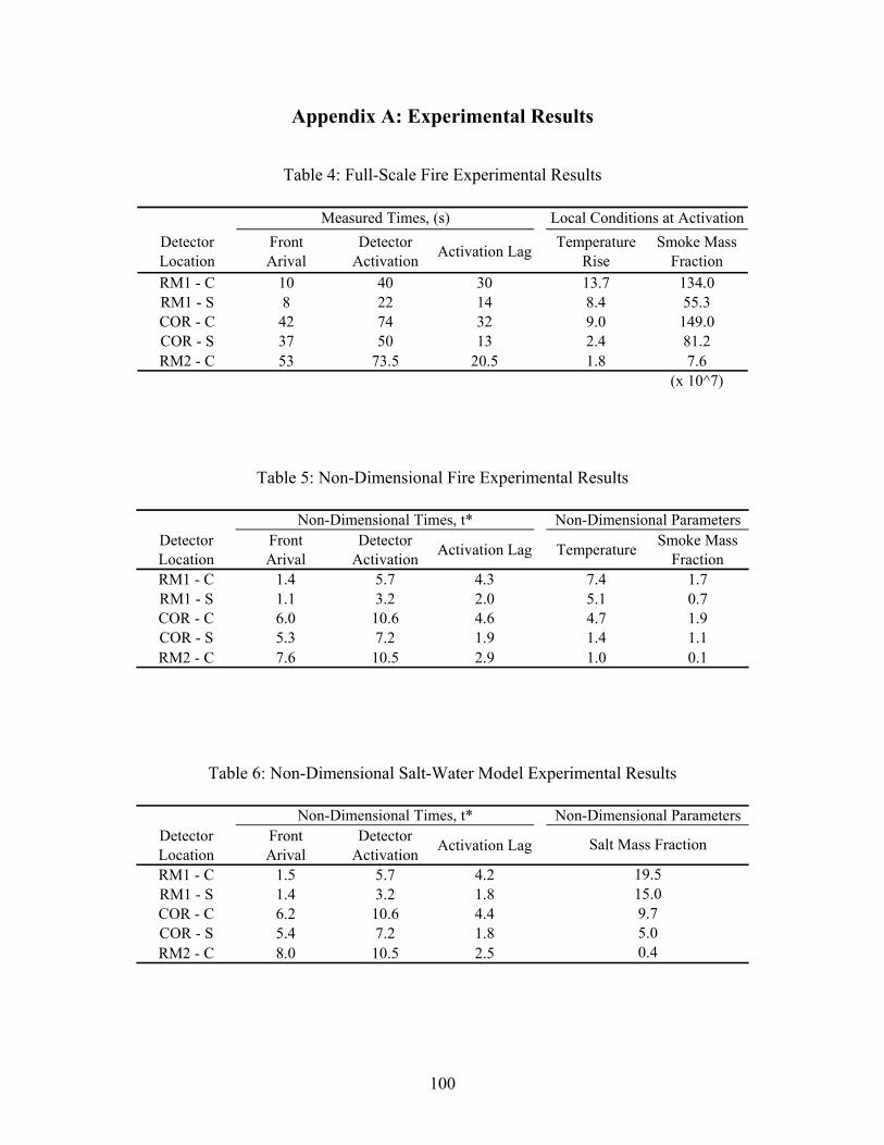
Appendix A: Experimental Results
Table 4: Full-Scale Fire Experimental Results
Detector Location
Front Arival
Detector Activation Activation Lag Temperature
Rise Smoke Mass
Fraction RM1 - C 10 40 30 13.7 134.0RM1 - S 8 22 14 8.4 55.3COR - C 42 74 32 9.0 149.0COR - S 37 50 13 2.4 81.2RM2 - C 53 73.5 20.5 1.8 7.6
(x 10^7)
Measured Times, (s) Local Conditions at Activation
Table 5: Non-Dimensional Fire Experimental Results
Detector Location
Front Arival
Detector Activation Activation Lag Temperature Smoke Mass
Fraction RM1 - C 1.4 5.7 4.3 7.4 1.7RM1 - S 1.1 3.2 2.0 5.1 0.7COR - C 6.0 10.6 4.6 4.7 1.9COR - S 5.3 7.2 1.9 1.4 1.1RM2 - C 7.6 10.5 2.9 1.0 0.1
Non-Dimensional Times, t* Non-Dimensional Parameters
Table 6: Non-Dimensional Salt-Water Model Experimental Results
Detector Location
Front Arival
Detector Activation Activation Lag
RM1 - C 1.5 5.7 4.2RM1 - S 1.4 3.2 1.8COR - C 6.2 10.6 4.4COR - S 5.4 7.2 1.8RM2 - C 8.0 10.5 2.5
Salt Mass Fraction
19.515.09.75.00.4
Non-Dimensional Times, t* Non-Dimensional Parameters
100

Appendix B: Check List
DATE: TEST#
------- EXPERIMENTAL ------------------------------------------ EXPERIMENTALTurn salt water pump on Dye Concentration (mg/l)Record salinity and temperature of the SW Salt Concentration (%)Circulate SW solution through tubes SW Temperature (C)Turn Laser On / record laser power Tank Water Temperature (C)Check spatial filter for proper alignment Laser powerCheck the vertical planar alignment Location of Max light from bottomCheck proper location of light distribution Injector Location -top (mm)Measure the frame and injector locations Gain value (o'clock)Place model on frame and adjust Brightness modAlign camera and ruler for scale (IMAGE) Noise (+/- GL)Adjust and Record brightness mod CJ Peak signal (GL)Hook up injector and run preliminary Flow settingAdjust flow to 40 and stop test Tube peak signal (GL)Adjust gain and record +/- noise and peak signal Background Noise (+/- GL)Recirculate water in tank tank Calibration Peak Signal (GL)Measure light profile of tube Calibration /max Gain Peak Signal (GL)Take background image record +/- noiseSplit background images!!Begin macro for data acq.Start flow and make sure it is ~ 40Mix calibration tank and record peak signal
------- POSTPROCESSING ----------------------------------------POSTPROCESSINGCreate and Save Background image Total number of imagesCreate and Save Calibration image Number of images prior to injectionSave final tiff's (gray scale) Threshold valueSave raw tiff's Cut valueSave .dat file Prenoise value
Scale (pixel/cm)X-initial
101

Appendix C: Experimental Procedure
Water Treatment The fresh water used to fill the large tank is filtered through a high capacity sediment and
rust filter. The filter is rated to 50-microns and allows a flow rate of 25 gallons per
minute. The purpose of this filtration is to remove any foreign particulate from the water
contained within the scale model and the large tank that would interfere with the light
sheet intensity. Water treatment is necessary for the salt-water solution as well, in order
to remove unwanted sediment and to reduce the hydrophobic reaction between the
Rhodamine dye and the water.
In preparing the saline solution, a large 40-gallon container is filled with warm tap water
in which a nylon bag filled with water softening rock salt (NaCl) is suspended in the
water. The salt is suspended and not just placed in the water to accelerate the mixing
process. The heavy salt water moves to the bottom of the container allowing the rock salt
to be exposed to fresh water, this natural convection allows the salt to completely
dissolve in the water without any forced mixing. The initial salt mixture is made at a
relatively high concentration, around 20 percent NaCl by mass. The high concentration
saline solution is then filtered from the large mixing tank to a secondary container where
the salt mass fraction is measured and adjusted accordingly by mixing in additional fresh
water. From the secondary container the saline solution is filtered once again into a 5-
gallon food grade plastic carboy. It has been observed by previous researchers that
residual chlorine reacts with Rhodamine 6G. The reaction causes a significant decay in
the dye concentration. The chlorine level of the solution is tested using a chlorine test kit
and the chlorine is removed by adding a small amount of de-chlorinating agent to the
102

solution. The mixture is agitated for several minutes, poured into the top section of the
gravity feed system, and mixed with the prescribed amount of Rhodamine 6G dye. The
inline filter used for the treatment of the salt-water solution is a carbon based sediment
and rust filter with a 5-micron rating and a maximum filtration rate of 5-gallons per
minute. The water is driven through the filter using a submersible salt-water fish tank
pump.
Dye Treatment Rhodamine 6G is used as the fluorescent dye for the PLIF diagnostics within this study.
The lab grade Rhodamine dye is 99.9% pure and is purchased in solid form from Lycros
Chemicals Inc. In pure form, the dye must be stored in a dry environment and kept away
from any ambient light. It is important to note, that prepared laser dye solutions usually
contain very minute amounts of dye. Thus, the type of solvent used as well as its purity is
of great importance. Impurities and additives may strongly effect the lifetime of the dye
and may catalyze photochemical reactions. For this reason distilled water is used as the
preliminary solvent. The pure dye is weighed using a precision digital scale with an
accuracy of ± .001 grams. An initial solution is made with a concentration of 0.1 grams
of dye per liter of solute, which is added, in liquid form, to the saline solution prior to
experimentation.
Gravity Feed System Prior to each experiment a 5 gallon volume of salt-water solution is prepared and the
salinity is measured using a hydrometer. The large fresh water tank is filled with filtered
tap water and the temperature is monitored, adjusted and recorded. The treated saline
103

solution is transferred to the top container of the gravity feed system and the temperature
is measured and recorded using a mercury/glass thermometer. The temperature of the
saline solution and the water within the enclosure is measure to assure that the density.
The necessary amount of concentrated dye solution is added to the treated salt-water and
agitated by hand with a glass-stirring rod to ensure proper mixing; the dye concentration
used is tabulated.
Optical Setup It should be noted that much care has been taken to maintain a stable optical set up for
creation of the light sheet, however, it is still necessary to ensure the optics are correct
prior to each experiment. The Argon-Ion laser is activated and the power is reduced to 40
mW for the duration of the optical alignment. The proper alignment of the spatial filter is
confirmed by placing a white piece of paper between the collimating lens and the spatial
filter. If the expanded beam is not perfectly round then adjustments must be made. Any
adjustment made to the spatial filter necessitates a realignment of the collimating lens.
This is done by; 1) changing the location of the collimating lens with respect to the
spatial filter, manually on the optical traverse system, and 2) placing two adjustable
apertures in the optical path beyond the lens to ensure the beam diameter remains
constant. After adjusting both the spatial filter and the collimating lens, the focus is
placed on the optical mirrors. Both mirrors are cleaned of excess dust and debris using an
optical cleaning cloth. The alignment of the optical mirrors is established by passing the
collimated beam through a series of adjustable apertures in the beam path beyond the
mirrors. Once this is complete the next step is to establish the proper position of the laser
sheet.
104

Laser Sheet Alignment Preliminary tests have been conducted to locate the optimal light sheet dimensions and
position, for each plane of interest with in the room-corridor-room model. Because of the
Gaussian light intensity distribution, the vertical location of the light sheet is of great
significance. It is important that the sheet is introduced in such a manner that the area of
most significance is adequately illuminated, while at the same time providing adequate
illumination through out the entire spatial domain. Several steps are required prior to
experimentation in order to assure the laser sheet is oriented properly. First, the
cylindrical lens is removed from the beam path and the vertical location of the beam is
measured, at two locations, from the top of the model frame within the large freshwater
tank; the values are compared to prior tests, adjusted, and recorded. The height and angle
of the horizontal beam is varied by carefully adjusting the optical mirrors. Next, the
cylindrical lens is replaced and the vertical planar alignment is conducted by passing the
laser sheet through a plum line. For the final step the laser power is set to 500 mW and
the light intensity distribution is tested. The laser sheet is passed through an acrylic
cylindrical tube filled with 0.02 mg/L of dye and vertically suspended from the large tank
at two specific locations. Instantaneous images are recorded and the light sheet
distribution is plotted. The profile is evaluated in two ways: 1) by the pixel location of the
maximum light intensity and 2) the distance from the max to 50% of the max. If
necessary the sheet is adjusted to match prior tests. If further adjustments are necessary
the power of the laser must be reduced.
Image Acquisition The polycarbonate scale model is placed on the positioning system within the large
freshwater tank. The CCD camera is positioned and adjusted based on the geometric view
105

factor of the planar sheet. Then, a standard stainless steel ruler is placed vertically in the
model within the path of the laser sheet. The camera is focused on the ruler and an image
is recorded to represent the physical scale of the test images. Next, the room lights are
turned off and the aperture of the camera is fully opened. Within the image acquisition
software the brightness modification is adjusted to ensure that the background noise is
greater then zero and the percent modification is tabulated.
Prior to the first experiment it is necessary to complete several steps that are not required
until the setup is changed. Firstly, the position of the injector is measured with calipers,
adjusted, and recorded. Secondly, the tube from the delivery system is connected to the
injector and a high flow rate of saline solution is sent through the lines to remove any air
bubbles present in the injector or in the lines. The flow rate is then adjusted to that
required for testing and the cameras gain is adjusted to prevent saturation.
Preceding each experimental run, a series of background images are recorded and the +/-
background noise values are tabulated. The image acquisition program is triggered prior
to the injection of the saline solution; the relative time is recorded and tabulated.
Following each experiment the new flow rate is adjusted and the water in the model is
recirculated until no dye is visible. After the experiments are conducted a series of
calibration images are recorded in which model is filled with a known dye concentration.
Only one average calibration image is needed for each series of tests representing a
geometric planar slice. Finally, the model enclosure is removed from the large tank and
replaced by a stainless steel injector. The injector is positioned slightly above the
106

maximum light intensity region of the laser sheet. Dyed salt-water is injected into the
tank at various dye and salt concentrations and an average of 300 images is taken. The
initial region of these forced plumes have a known salt and dye concentration and can be
used to determine the effect of salt on the fluorescence intensity. This effect is included in
calibration. The respective values for the dye concentrations and salt mass fractions are
reported.
Converting Raw Tiff Images The captured images are saved in binary format, in which the two consecutive images for
each time step are contained in a single binary file. A macro written within the data
acquisition program is used to separate the files, convert them into tiff images, and assign
a proper file name accordingly. The calibration and background binary files are separated
into a series of tiff images as well. The raw tiff images are then transferred to an ftp file
server in which they are backed up and are now accessible to the university’s Unix based
servers. The program X-Win32 is used to gain access to the Unix servers from a
Windows based PC. Within the Unix server a temporary directory is created from which
the raw tiff images are transferred.
Processing Data Several procedures have been written in the international data language program (IDL)
for post processing and analysis. The foundation of these programs is based on
converting an 8-bit tiff image into quantitative data. The images are read in and then each
row and column is scanned allowing the grayscale for each pixel within the image to be
converted into a numerical array. For the first stage of post processing a program reads in
the raw background images and combines them into a single average background image
107

that is saved for further data analysis. Taking the average of several hundred images
allows the digital noise to be removed, leaving only the noise associated with the
enclosure itself. A similar program is used to create an average calibration image. The
program subtracts out the average background image prior to saving the average
calibration image. The calibration image allows the laser sheet profile to be quantified
spatially thus providing a means to normalize the experimental images.
The instant image code is somewhat complex and is used as one of the final steps in
processing the data. Prior to normalization there are several steps that must be preformed
in order to create a clean image with sufficient depth. The following parameters are input
variable defined by the user:
CUT – defines the maximum multiplication factor from the light sheet
THRESH – defines the minimum value that the normalized image can have
PRENOISE – defines a minimum value for the image prior to normalization
CJPOINTVALUE – defines the grayscale value of a specified point of interest which
creates an image multiplication factor
SCALE – defines length scale in terms of the amount of pixels in one centimeter
ORIGINX – defines the initial x-location of the image
ORIGINY – defines the initial y-location of the image
TIMESHIFT – defines the time lapse prior to the flow of saline solution
Using the scale image taken prior to the experiment, the pixel location of the enclosures
origin and the actual ratio of the image in pixels to the model in centimeters can be
108

obtained. These are the first values to be defined by the user in the instant image post
processing code. The program is written to map out the boundaries of the enclosure for
all specific configurations as well as the location of the probes representative of the
smoke detectors in the full-scale experiment. There are several input parameters that
define the experimental configuration and the manor in which the raw images will be
processed.
To input the proper values for post processing it is necessary to first load up a set of
images that is representative of a steady state flow. The program can be run and the
processed image can be evaluated. Adjusting the CUT, THRESH, and PRENOISE values
before running the entire set of test data allows the bounds of the normalized image to be
set by the user and removes the digital noise from the raw images prior to the
normalization. Once these inputs are optimized, the CJPOINTVALUE is set to prescribe
an acceptable gray level at a specific point of interest. For a ceiling jet flow that is
downstream of the impinging plume, a gray scale value of 100 out of 255 is acceptable
for the research at hand. The program will then process the steady state image and output
a multiplication factor for the entire spatial domain based on the prescribed gray level.
This assures that finalized images will have good resolution within the area of interest.
Due to the fact that the testing requires the image acquisition to begin prior to the
introduction of the saline solution, it is necessary for the time lapse to be an input
parameter within the code. This allows the program to save the images with a time stamp
resembling the time from the initial introduction of the source.
109

The “instant images” program uses several steps in order to process the raw images. The
program first reads in both consecutive images for each time step and converts the images
into two numerical arrays. Since the images taken are interlaced the program is written to
read every other row of the array and stretch the values to fill the original spatial
coordinates. Now there are four arrays/images representative of a single time step. These
images are then added together and the average background image is subtracted. A
multiplication factor is applied to the clean images to correct for the Gaussian light
intensity distribution. The program creates the multiplication factor for the entire spatial
domain by loading the average calibration image in as a numerical array and dividing the
maximum gray level by this entire array. Finally, the corrected gray level values are
converted into values representative of the salt mass fraction by applying a third order
polynomial interpolation. The computation repeated for each time step of the experiment.
Output Parameters The program is written to output the processed data in several formats. The final and
clean images, in terms of gray level, are saved as tiff images for each respective time
step. A data file is also created to allow the quantitative images to be open in TecPlot.
The data file consists of the spatial coordinates of each pixel, the gray level value, the salt
mass fraction, the non-dimensional salt mass fraction, and the non-dimensional time (for
probe locations). The point measurements made at the relative locations of each smoke
detector are presented in terms of non-dimensional mass fraction vs. non-dimensional
time, which are used in comparison with the full-scale test results.
110

Bibliography 1. Munson, B. R., Young D. F. and Okiishi T.H., (1998) “Fundamentals of Fluid
Mechanics,” 3rd Ed., John Wiley and Sons, New York. 2. Drydale, D.D., (1998) “ An Introduction to Fire Dynamics,” 2nd Ed., John Wiley
and Sons, New York.
3. Worrell, C.L., Lynch, J.A., Jomass, G., Roby, R.J. (2003) “Effect of Smoke Source and Horn Configuration on Enhanced Deposition, Acoustic Agglomeration, and Chladni Figures in Smoke Detectors,” Fire Technology, 39, pp. 309-346.
4. Thomas, P.H., Hinkley, P.L., Theobald, C.R. and Simms, D.L., (1963)
“Investigations into the Flow of Hot Gases in Roof Venting,” Fire Research Technical Paper No. 7, HMSO, London.
5. Tangren, E. N., Sargent, W. S. and Zukoski, E. E., (1978) “Hydraulic and
Numerical Modeling of Room Fires,” California Institute of Technology, Pasadena, California.
6. Zukoski, E.E, (1978) “Prediction of Smoke Movement in Buildings,” California Institute of Technology, Pasadena, Ca.
7. Steckler, K.D, Baum, H.R., and Quintiere, J.G (1986) “ Salt Water Modeling of
Fire Induced Flows in Multi-Compartment Enclosures,” NBSIR 86-3327, Gaithersburg, MD: National Bureau of Standards.
8. Kelly, A. A. (2001) “Examination of Smoke Movement in a Two-Story
Compartment Using Salt Water and Computational Fluid Dynamics Modeling,” M.S. Thesis, Dept. Fire Protection Engineering, University of Maryland, College Park, MD.
9. Webster, D.R. and Liu, Y. (2001) "Velocity Measurements of Turbulence
Collapse in a Linearly Stratified Jet," Experiments in Fluids, vol. 31(4), pp. 394-400.
10. Houssine, I., Vivier, H., Plasari, R. and Villermaux, J. (1996) “Planar laser
induced fluorescence technique for measurements of concentration fields in continuous stirred reactor tanks,” Exp. Fluids, Vol. 22, pp. 95 – 102.
11. Fukushima, C., Aanen, L., Westerweel, J. (2000) “Investigation of the Mixing
Process in an Axisymmetric Turbulent Jet Using PIV and LIF,” Laboratory for Aero and Hydrodynamics, Delft University of Technology, The Netherlands.
112

12. Lengricht, J. and Graw, K-U. (1995) “Flow Field Analysis Beneath Gravity Waves. In: Flow Visualization and Image Processing of Multiphase Systems,” ASME, FED 209, pp. 57 – 64. New York.
13. Law, A.W. K. and Wang, H. (2000) “Measurement of mixing processes with
combined digital particle image velocimetry and planar laser induced fluorescence”, Exp. thermal and Fluid Science, 22, 213-229.
14. Peters, W.D., Codswell, S.R., and Venart, J.E.S (1997) “Mixing in Gravity
Current Heads Flowing Over Rough Surfaces,” Developments in Laser Techniques and Fluid Mechanics, Eds. R.J. Adrian et al., Springer Berlin, Ch. III, pp. 325 – 339.
15. Clement, M.J. (2000) “Experimental Verification of the Fire Dynamics Simulator
(FDS) Hydrodynamic Model,” PhD Thesis Draft, University of Canterbury, New Zealand.
16. Baum, H.R., Rehm, R.G. (1984) “Calculations of Three Dimensional Bouyant
Plumes in Enclosures,” National Bureau of Standards, Washington, DC.
17. Rehm, R.G, Baum, H.R (1978) “The Equations of Motion for Thermally Driven Buoyant Flows,” N.B.S J. Res. 83, 297.
18. Turner, J.S. (1973) “Buoyancy Effects in Fluids,” Cambridge University Press,
Cambridge. 19. Morton, B.R., Taylor, G.I., and Turner, J.S. (1956) “Turbulent Gravitational
Convection from Maintained and Instantaneous Sources,” Proc. of the Royal Society of London, Vol. 234, Issue 1196, pp. 1 – 23.
20. Dai, Z., Tseng, L.K., and Faeth, G.M. (1994) “Structure of Round, Fully-
Developed, Buoyant Turbulent Plumes,” Journal of Heat Transfer, Vol. 116, pp. 409-417.
21. Morton, B.R. (1959) “Forced Plumes,” Journal of Fluid Mechanics, Vol. 5, pp.
151 - 163.
22. Heskestad, G. and Delichatsios, M.A., (1977) “Enviornments of Fire Detectors – Phase I: Effect of Fire Size, Ceiling Height and Material,” Volume I and II, National Bureau of Standards, Gaithersburg, MD.
23. Schifiliti, R. P. and Pucci, W. E. (1996) “Fire Detection Modeling: State of the
Art,” Fire Detection Inst., Bloomfield, CT, p. 57.
113

24. Bukowski, R. W. and Averill, J. D. (1998) “Methods for Predicting Smoke Detector Activation,” Building and Fire Research Laboratory, National Institute of Standards and Technology, Gaithersburg, MD 20899, USA.
25. Evans, D. and Stroup, D., (1985) “Methods to Calculate the Response Time of
Heat and Smoke Detectors Installed Below Large Unobstructed Ceilings,” NBSIR 85-3167, National Bureau of Standards, Gaithersburg, MD.
26. Milke, J. A., (1990) “Smoke Management for Covered Malls and Atria,” Fire
Technology, Vol. 26, No. 3, pp. 223 - 243.
27. Beyler, C. and DiNenno, P., (1991) “Letters to the Editor,” Fire Technology, Vol. 27, No. 2, pp. 160 – 169.
28. Davis, W.D. and Notarianni, K.A., (1996) “NASA Fire Detector Study,” NISTIR
5798, National Institute of Standards and Technology.
29. Mowrer, F.W. and Friedman, J., (1998) “Experimental Investigation of Heat and Smoke Detector Response,” Proceedings of Fire Suppression and Detection Research Application Symposium, pp. 256 – 264.
30. Geiman, J. A. and Gottuk, D. T., (2003) “Alarm Thresholds for Smoke Detector
Modeling,” Fire Safety Science – Proceedings of the 7th International Symposium, International Association for Fire Safety Science, pp. 197 – 208.
31. Schifiliti, R.P., Meacham, B.J. and Custer, R.L.P., (2002) “Design of Detection
Systems,” SFPE Handbook of Fire Protection Engineering, 3rd edition, National Fire Protection Association, Quincy, MA.
32. Geiman, J.A., (2003) “ Evaluation of Smoke Detector Response Estimation
Methods,” Masters Thesis, University of Maryland Department of Fire Protection Engineering.
33. Bukowski, R.W. and Mulholland, G.W., (1978) “Smoke Detector Design and
Smoke Properties: Final Report,” NBS Technical Note 973, National Bureau of Standards, Gaithersburg, MD.
34. Cleary, T., Chernovsky, A., Grosshandler, W. and Anderson, M., (2000)
“Particulate Lag Entry in Spot-Type Smoke Detectors,” Fire Safety Science – Proceedings of the 6th International Symposium, International Association for Fire Safety Science, pp. 779 –780.
35. Bejan, A. (1984), “Convection Heat Transfer,” Wiley Publications, New York.
36. Chandrasekhar, S. (1957), “An Introduction to the Study of Stellar Structure,”
New York: Dover
114

37. Walker, D.A. (1987), “A Fluorescence Technique for Measurements of
Concentration in Mixing Liquids,” Journal of Physics E: Scientific Instruments, Vol. 20, pp. 217 – 224.
38. Guilbault, G.C. (1973) “Practical Fluorescence,” New York: Marcel Dekker.
39. Arcoumanis, C., McGuirk, J.J., and Palma, L.M. (1990) “On the Use of
Fluorescent Dyes for Concentration Measurements in Water Flows,” Experiments in Fluids, Vol. 10, pp. 177 – 180.
40. Davidson, M.J., Pun, K.L., Wang, H.J. (1997) “Applications of laser induced
fluorescence and image processing in observing plume behavior.” Proc. 3rd Int. Conf. On Fluid Dynamic Measurements and its Applications, International Academic, Beijing, China.
41. Barbrauskas, V. (1995) “The cone calorimeter,” SFPE Handbook of Fire
Protection Engineering, 2nd Edition, pp. 3.37 – 3.52, Society of Fire Protection Engineering, Boston.
115