Embed Size (px)
Citation preview
ABSTRACT
Title of thesis: NEGATIVE CONSTRUCTION SECTORS THAT
INFLATE GROSS DOMESTIC PRODUCT: AN ECONOMIC CASE STUDY OF SEATTLE COMMERCIAL CONSTRUCTION
Jeffrey James Christianson, Master of Science, 2014 Thesis directed by: Professor Qingbin Cui Department of Civil and Environmental Engineering
Gross Domestic Product (GDP) was created as a way to measure US production
of products and services. GDP was not intended to guide policy making or as an indicator
of the country’s welfare. The commercial construction sectors of asbestos abatement, soil
remediation, and building demolition are tangential to the actual cost of constructing a
building and the country would be better off if these construction sectors were not
necessary, even at the jeopardy of a reduced GDP.
This thesis examines the specific costs of these construction sectors in Seattle
commercial construction industry and determines that 1.66 percent of a Seattle
commercial construction project’s cost is spent on asbestos abatement, soil remediation,
and building demolition. This research challenges the use of GDP and emphasizes the
need for a different means to measure economic progress in consideration of the incurred
environmental and social costs in the production of products and services.

NEGATIVE CONSTRUCTION SECTORS THAT INFLATE GROSS DOMESTIC PRODUCT: AN ECONOMIC CASE STUDY OF SEATTLE COMMERCIAL
CONSTRUCTION
by
Jeffrey James Christianson
Thesis submitted to the Faculty of the Graduate School of the University of Maryland, College Park in partial fulfillment
of the requirements for the degree of Master of Science
2014
Advisory Committee: Professor Qingbin Cui, Chair Professor Gregory Baecher
Professor Miroslaw Skibniewski

© Copyright by
Jeffrey James Christianson
2014

ii
TABLE OF CONTENTS
List of Figures ................................................................................................................................. iv
List of Tables ................................................................................................................................... v
Chapter 1: Introduction ................................................................................................................... 1
Introduction .................................................................................................................................. 1
Problem Statement ....................................................................................................................... 2
Research Objectives ..................................................................................................................... 3
Hypothesis ................................................................................................................................... 3
Implications ................................................................................................................................. 4
Thesis Format .............................................................................................................................. 4
Chapter 2: Background .................................................................................................................... 7
Introduction .................................................................................................................................. 7
Progress Measurements ............................................................................................................... 8
GDP History ............................................................................................................................ 8
GDP Methodology ................................................................................................................. 10
Construction Value Added ..................................................................................................... 11
GDP Facts and Figures .......................................................................................................... 12
Alternative Economic Measurements .................................................................................... 16
Other Indicators ..................................................................................................................... 17
Economics .................................................................................................................................. 19
United States Economic Growth ............................................................................................ 19
United States Economic Recessions ...................................................................................... 21
Construction Recessions ........................................................................................................ 23
Construction Sector Assessment ................................................................................................ 24
Introduction ............................................................................................................................ 24
Asbestos Abatement ............................................................................................................... 25

iii
Building Demolition .............................................................................................................. 28
Contaminated Soil Remediation ............................................................................................ 30
Chapter 3: Research Methodology ................................................................................................ 35
Questionnaire Design ................................................................................................................. 35
Sampling .................................................................................................................................... 37
Processing Survey Responses .................................................................................................... 41
Additional Information .............................................................................................................. 41
Chapter 4: Research Results ......................................................................................................... 43
Results ........................................................................................................................................ 43
Contaminated Soil .................................................................................................................. 46
Building Demolition .............................................................................................................. 47
Asbestos Abatement ............................................................................................................... 48
Analysis ..................................................................................................................................... 49
Contaminated Soil .................................................................................................................. 49
Building Demolition .............................................................................................................. 50
Asbestos Abatement ............................................................................................................... 51
Chapter 5: Discussion ................................................................................................................... 53
Conclusion ................................................................................................................................. 53
Research Limitations ................................................................................................................. 55
Recommendations ...................................................................................................................... 57
APPENDICES ............................................................................................................................... 59
Appendix A: Yearly GDP Figures ............................................................................................ 59
Appendix B: 2008-2009 NAICS Sector Earnings Variance ..................................................... 65
Appendix C: Survey Form ........................................................................................................ 66
Appendix D: Additional Survey Project Information ............................................................... 69
Appendix E: Survey Data Calculations .................................................................................... 70
REFERENCES .............................................................................................................................. 75

iv
List of Figures
FIGURE 2-1. United States Gross Domestic Product (GDP) in dollars since 1929. ....... 13 FIGURE 2-2. United States construction sector’s yearly value added to Gross Domestic Product (GDP) in dollars since 1947 ................................................................................ 14 FIGURE 2-3. United States construction sector’s yearly value added to Gross Domestic Product (GDP) as a percent from 1947-2012 ................................................................... 14 FIGURE 2-4. Percentage variance between current year and previous year from 1947- 2012 of Gross Domestic Product and the construction sector’s value added to Gross Domestic Product. ............................................................................................................. 15 FIGURE 2-5. United States Gross Domestic Product (GDP) versus Genuine Progress Indicator (GPI) per capita from 1950-2004 using 2000 chain dollars .............................. 17 FIGURE 3-1. Project start year distribution of projects surveyed. .................................. 38 FIGURE 3-2. Project type distribution of projects surveyed. .......................................... 40 FIGURE 3-3. Project survey respondent type distribution. ............................................. 40 FIGURE 4-1. Standard deviation of contaminated soil remediation costs as a percentage of construction value for Seattle commercial construction projects surveyed. ................ 47 FIGURE 4-2. Standard deviation of building demolition costs as a percentage of construction value for Seattle commercial construction projects surveyed. ..................... 48 FIGURE 4-3. Standard deviation of asbestos abatement costs as a percentage of construction value for Seattle commercial construction projects surveyed. ..................... 49 FIGURE 4-4. Location of Seattle commercial construction projects surveyed ............... 52

v
List of Tables
TABLE 2-1. North American Industry Classification System (NAICS) sectors ............ 11 TABLE 4-1. Costs in dollars and as a percentage of project construction value for asbestos abatement, soil remediation, and building demolition for Seattle commercial construction projects surveyed. ......................................................................................... 44 TABLE A-1. Yearly United States Gross Domestic Product from 1929-2013 in dollars and the construction sector’s yearly value added to Gross Domestic Product from 1947-2012 in dollars and as a percent. ....................................................................................... 59 TABLE A-2. Delta between current year and previous year Gross Domestic Product and the delta between current year and previous year of construction sector’s value added to Gross Domestic Product. .................................................................................................. 62 TABLE B-1. Delta between 2008 and 2009 value added to Gross Domestic Product organized by North American Industry Classification System (NAICS) sector code. ..... 65 TABLE D-1. Project start date and building type for projects surveyed ......................... 69
1
Chapter 1: Introduction
Introduction
During The Great Recession of 2008-2009, the United States government shelled
out billions of stimulus dollars to the construction industry in an effort to impede further
recession and spur recovery. But, should the government be creating polices in an effort
to maximize Gross Domestic Product (GDP)? Construction activities that do not enhance
the wellbeing of people should not be striven to maximization because they do not
represent what is best for a country.
Not all construction spending signifies a good thing. There are several
construction activities that do not denote progress as a country or contribute to personal
enrichment as individuals. It should not be our goal as a country to maximize spending on
construction defect repair, natural disaster rebuilding, vandalism or smoke damage
restoration, brownfield cleanup, asbestos abatement, or building demolition. The more
money that is spent on these items represents the frequency of their occurrence. The
welfare of the country would be better off if these situations did not occur, thus not
necessitating their repair/cleanup.

2
Problem Statement
While Gross Domestic Product is a good statistic to track the dollar amount of
goods and services produced, it should not be used as a beacon in establishing
governmental policies. In a 1968 speech given by Robert Kennedy at the University of
Kansas, he was quoted as saying Gross Domestic Product ‘measures everything in short,
except that which makes life worthwhile.’ There are many other enriching life
experiences that GDP cannot measure such as an individual’s happiness, spending time
with one’s family and friends, personal health, education, and community connection.
One of the leading advocates for an alternative progress measuring system is Dr.
Robert Costanza. Dr. Costanza is a Chair in Public Policy at the Crawford School of
Public Policy at Australian National University. Dr. Costanza’s research has focused on
sustainable development and alternative progress measurement indicators. His work has
been instrumental in getting the world to think about the cost of economic activity on
human welfare, the environment, and earth’s natural resources.
While Dr. Costanza’s work addresses the global implications of society’s general
disregard for the auxiliary costs of economic advancement and consumerism, there is
little data or research on the construction industry’s culpability to this problem. Three of
the most common construction sectors that have emerged in order to correct past policy
failures and industry deficiencies are asbestos abatement, building demolition, and
contaminated soil remediation.
Currently, there is not an economic reporting system in place to track the amount
of money spent on asbestos abatement, soil remediation, and building demolition as it
specifically relates to construction. Without these specific figures, the United States GDP

3
continues to misrepresent the progress that the country is making and the quality of life
available to its citizens.
Research Objectives
This thesis will examine asbestos abatement, building demolition and
contaminated soil remediation and what they ‘contribute’ to commercial construction
costs in the Seattle market. Data will be collected through project surveys of recently
completed jobs. Through this data, the author will be able to identify what percentages of
construction costs in Seattle are as a result of these three non-welfare enhancing
activities.
This research will representative of how certain industries should not be
proliferated nor encouraged. It will indicate how certain sectors of business are necessary,
however their maximization shouldn’t be considered when making policies and laws
about what is best for the citizens of the United States.
Hypothesis
The United States economy is bolstered by economic activities that are
necessitated by the need to rectify the repercussions of past policy failures. When these
economic activities are removed from the GDP, the country’s output looks less
prosperous. However, prosperity is contextual when other personnel values are
considered. The Seattle real estate development and commercial construction industry is
laden with imposed costs for soil remediation, asbestos abatement, and building
demotion. These costs inflate the Seattle economic figures and consequently, the United
States GDP as well.

4
Implications
It is important to discern a countries economic activity that enhances the
wellbeing of its citizens and those activities that create or sustain a mediocre existence.
Just like a business’s profits are calculated based on revenue minus expenses, a countries
growth should also consider the social and environmental costs of the output.
This information is significant because society is changing. One of the visions
that came out of the United Nations Conference on Sustainable Development in 2012 was
the ‘need for broader measures of progress to complement GDP in order to better inform
policy decisions’ (United Nations 2012). In the near future, the cost of industry and
production on the environment and society will no longer be an unheeded byproduct.
The quantification of Seattle commercial construction dollars spent on asbestos
abatement, building demolition, and soil remediation will show what percentage these
three sectors make-up of the dollars spent on commercial construction in Seattle. These
figures will demonstrate how these three sectors inflate the Seattle commercial
construction economy and will hint perhaps at how they also influence national GDP
figures. This data will support the global movement for an alternative measurement of
progress and development, including the construction industry.
Thesis Format
After this introduction section, the thesis is broken out into four subsequent
chapters. The Background chapter will provide the history of GDP and why it became
such a prominent indicator in the United States’ economy. The GDP calculation methods
will be discussed as well as what contributions the construction industry makes to GDP.

5
Historical GDP figures will be evaluated and the world events that influenced the cyclical
highs and lows of GDP. Alternative economic measurements and other progress
indicators are presented. A historic examination of asbestos abatement, building
demolition, and contaminated soil remediation will take place and why these sectors are
in existence today. Past costs of these industries will be discussed and what the future
costs are expected to be.
The next chapter is Research Methodology. This chapter will discuss how data
was collected for this thesis and the sources of the data. The evaluation methods of the
data are explained as well as some of the difficulties encountered during the research.
The Research Results chapter presents the data from the research and highlights
the dispersion of projects evaluated. The mean and standard deviation of the asbestos
abatement, building demolition, and soil remediation figures are presented and evaluated.
Data outliers are examined and how they influenced the mean and standard deviation
calculations.
The final chapter is the Discussion section. This chapter presents a conclusion
based on the research data. Limitations of the research and the ability of the Seattle data
collected to be generalized throughout the United States are examined. The Research
Limitations subsection also discusses factors that could influence the research data and
criteria that is included or excluded from the evaluation of the data. The chapter will
close with recommendations on what context GDP should be held in and suggestions on
how the data presented in this thesis can be used to spur discussion on measuring what is
important to the United States citizens in the 21st century.

6
The Appendices section contains GDP historical data as well as data for the
construction industry value added to GDP. A copy of the project survey form is included
as well as supplemental information to Chapter 4 project information. The final appendix
section covers the different calculations for the mean and standard deviation figures
presented in Chapter 4.

7
Chapter 2: Background
Introduction
Gross Domestic Product is the value of products and services produced within the
United States. GDP is typically seen by the government and economists as an economic
health indicator of the country. Since the GDP was created, it has been the goal of the
United States to continuously increase the GDP annually.
This chapter discusses the history of GDP and why it was created. It explores the
means and methods for calculating GDP and how the different business sectors bring
together the GDP figure. Past GDP figures are assessed and the construction sector is
specifically delved into and what its contribution historically has been to GDP. Economic
growth and recession years are examined and the different events that influenced these
economic activities are reviewed.
In addition to GDP, there are several other progress measurements that are
sparingly in use throughout the world for various purposes. Some of the indicators aim to
take the place of GDP by adjusting economic measurements to account for social and
environmental factors. Other measurements are composite measurements that consider
economic prosperity while also considering well-being indicators. There are also
subjective survey measurements (Costanza et al. 2014). These three alternatives to GDP
are evaluated. The chapter is concluded by examining the history and defining the three
negative construction sectors that are the focus of this thesis research: asbestos
abatement, soil remediation, and building demolition.
8
Progress Measurements
GDP History
Gross Domestic Product (GDP) was originally referred to as Gross National
Product (GNP). GNP was the dollar value of products and services produced by residents
of a country (regardless of what country the work was conducted in). GNP was replaced
by GDP in 1991 and is the dollar value of products and services produced within a
country’s boarders (regardless if it is by a foreign company).
GNP was created by Simon Kuznets. Kuznets was born in Russia in 1901 to
Jewish parents. His family fled the civil war in his home country in 1922 and immigrated
to the United States where he attended Columbia University. Kuznets studied economics
at Columbia University where he graduated with a PhD in 1926. After graduating, he
went to work for the National Bureau of Economic Research (NBER).
In the 1930’s, the world experienced the Great Depression. The United States
government knew of little action that could be taken to combat the rapid decline of
employment, international trade, and taxable income. Because no system of national
accounts existed prior to the Great Depression, the steps that were taken by the Herbert
Hoover administration to deal with the crises reaped no quantifiable improvements
(because there was no way to compare the before and after economic conditions). The
NBER was implored by the subsequent Roosevelt administration to create an economic
measuring system that the government could use to monitor the economic state of the
country. With the creation of the GNP, the government was able to measure the
effectiveness of their policy changes in order to pull the country out of an economic
tailspin. When Kuznets created a single GNP number, the government was able to track

9
what was collected, what was needed, what was spent, and what was earned, thus
enabling the proactive management of the cyclical business cycles that had plagued the
nation into the Great Depression (Fioramonti 2013).
Near the end of the Great Depression, World War II was in full swing. While
other countries were immediately forced into battle to protect their domestic and foreign
interests, the United States’ engagement was a little more calculated. Kuznets went to
work for the Planning Committee of the War Production Board in 1942. Through his
earlier work at the NBER and the creation of GNP, Kuznets was able to estimate the
country’s capacity to produce the necessary materials and equipment that would be
needed for the long war, and when those items would be available (Fioramonti 2013).
After World War II, the United Nations adopted the GNP as the primary
measurement of economic performance in the world. With this, all countries were able to
measure their economies and production against other countries. GNP soon became the
dominant weapon during the Cold War era.
The Cold War was a 40 year political battle between the two post-war
superpowers; the United States and USSR. This battle primarily comprised of the
escalation of industrialization and production. Just like GNP was utilized during World
War II, the United States went to great effort to discredit USSR economic figures as well
as predict their potential weaponry manufacturing capacity.
Under increased scrutiny of their economic calculation system, the USSR reached
out the United States Bureau of Economic Analysis in 1988 for help in revising their
measuring system. Once their calculation methods aligned with the United States, the true

10
picture of economics under communist rule was painted. Shortly thereafter, USSR’s
socialist economy collapsed making way for the market economy they have today.
GDP Methodology
Gross Domestic Product statistics and data is collected and managed in the United
States by United States Census Bureau (USCB). This data is provided in reports
generated quarterly, yearly, and every five years. The most comprehensive report is
referred to as the Economic Census which is conducted every five years; the latest being
held in 2012, though the data for this survey is not yet available.
The census data collected includes: kind of business, location, type of ownership,
total revenue, payroll, and number of employees (Economic Census n.d.). The data is
collected via mail surveys to every business with paid employees. The data collected is
used to generate both a comprehensive GDP figure for that given year, but also to
generate a benchmark that can be used to index estimates for subsequent years (as well as
quarters) until the next census.
Quarterly and yearly GDP figures are generated through surveys (a small portion
of the overall businesses) as well as through extrapolation of past information while
considering current known information (trends). As real data from monthly and quarterly
surveys is generated, revisions of the GDP are issued (Landefeld et al 2008).
The USCB seperates expenditures into four broad categries: consumption,
investment, government, and net exports (Landefeld et al. 2008). Addtionally, the USCB
classifies business types through the North American Industry Classifcation System
(NAICS). There are currently 20 sectors recognized by the USCB as shown in Table 2-1.

11
TABLE 2-1. North American Industry Classification System (NAICS) sectors
Sector Industry Title
11 Agriculture, forestry, fishing, and hunting 21 Mining 22 Utilities 23 Construction
31-33 Manufacturing 42 Wholesale trade
44-45 Retail trade 48-49 Transportation and warehousing
51 Information 52 Finance and insurance 53 Real estate and rental and leasing 54 Professional, scientific, and technical services 55 Management of companies and enterprises 56 Administrative and waste management services 61 Educational services 62 Health care and social assistance 71 Arts, entertainment, and recreation 72 Accommodation and food services 81 Other services, except government 92 Public Administration
Data adapted from: United States Department of Commerce: Bureau of Economic Analysis, GDP by Industry: 1997-2012 (2014)
Construction Value Added
The construction sector (which is part of the investment expenditure category)
consists of over 70 subsectors and industry groups. Additionally, there are several other
sectors that relate to construction including sector 22 (utilities), 53 (real estate), and 56
(remediation services). Industry data for the construction sector is collected through a
number of different surveys including the Economic Census, Building Permit Survey,
Value of Construction Put in Place, and Annual Capital Expenditures Data.
The Building Permit Survey is used to provide monthly and annual statistics on
privately-owned residential construction. Monthly surveys of 9,000 selected permit-

12
issuing places and yearly surveys of an additional 11,000 selected permit-issuing places
are used to compile the Building Permit Survey. The data collected from the Building
Permit Survey includes: number of buildings, number of housing units, and permit
valuation (Economic Census n.d.).
The Value of Construction Put in Place survey is used to provide monthly
estimates of the total dollar value of construction work (Economic Census n.d.).
Information for the survey is collected via monthly mail surveys and interviews with
project owners; consisting of 8,500 private non-residential projects, 8,500 state/local
projects, 2,500 apartment projects, and 700 federal projects. The data collected from this
survey includes: cost of labor and materials, cost of architecture and engineering, interest
on loans, as well as contractors overhead, profit, and taxes.
The Annual Capital Expenditures Survey provides yearly spending statistics on
new and used structures/equipment. Data is collected via mail surveys to 46,000
companies with one or more employees as well as 15,000 companies without any
employees. Additionally, all companies that have more than 500 employees participate in
the survey (Economic Census n.d.).
GDP Facts and Figures
Gross Domestic Product has seen its ups and downs since it was created,
although, the economic swings are not as severe as they would be if GDP did not exist.
GDP provides the government indicators they need to make informed economic policies
(Fioramonti 2013). Table A-1 shows what the national GDP has been over the past 85
years and what the construction sector has contributed to the GDP over the past 67 years.
Industry specific data is not available before 1947. Since the construction industry has

13
been tracked, its yearly value added to GDP has averaged 4.30 percent with a low of 3.52
percent in 2011 and a high of 5.04 percent in 2006.
Figure 2-1 compares the total GDP in current dollars (at that measured year) to
2009 chained dollars. Chained dollars are adjusted figures based on inflators and
deflators (Seasonal Adjustment of Chained Dollars n.d.). By using chained dollars, it
creates a baseline that is comparable against historical figures. Figure 2-2 compares
construction value added to GDP in current dollars to 2009 chained dollars and Figure 2-
3 shows what percentage construction contributed to the total GDP.
FIGURE 2-1. United States Gross Domestic Product (GDP) in dollars since 1929. Note: Data adapted from United States Department of Commerce: Bureau of Economic Analysis, Current-Dollar and "Real" Gross Domestic Product (2014).
$0
$2,000
$4,000
$6,000
$8,000
$10,000
$12,000
$14,000
$16,000
$18,000
1929
1934
1939
1944
1949
1954
1959
1964
1969
1974
1979
1984
1989
1994
1999
2004
2009
DO
LL
AR
S (
in b
illi
on)
YEAR
Current dollars
2009 Chaineddollars

14
FIGURE 2-2. United States construction sector’s yearly value added to Gross Domestic Product (GDP) in dollars since 1947. Note: Data adapted from United States Department of Commerce: Bureau of Economic Analysis, GDP by Industry: 1947-1997 (2014) and United States Department of Commerce: Bureau of Economic Analysis, GDP by Industry: 1997-2012 (2014).
FIGURE 2-3. United States construction sector’s yearly value added to Gross Domestic Product (GDP) as a percent from 1947-2012. Note: Data adapted from United States Department of Commerce: Bureau of Economic Analysis, GDP by Industry: 1947-1997 (2014) and United States Department of Commerce: Bureau of Economic Analysis, GDP by Industry: 1997-2012 (2014).
$0
$100
$200
$300
$400
$500
$600
$700
$800
1947
1952
1957
1962
1967
1972
1977
1982
1987
1992
1997
2002
2007
2012
DO
LL
AR
S (
in b
illi
on)
YEAR
Currentdollars
2009 Chaineddollars
0%
1%
2%
3%
4%
5%
6%
1947
1952
1957
1962
1967
1972
1977
1982
1987
1992
1997
2002
2007
2012
PE
RC
EN
TA
GE
YEAR

15
The construction sector’s contributions to GDP have been variable and with a few
exceptions, have followed the trend of the overall GDP peaks and valleys. Table A-2
reflects the dollar variances in total GDP and construction’s value added to GDP from
year to year as well as the percentage variances. The table shows a substantial growth
correlation in the early 1950’s, late 1960’s, early 1970’s, and 1984, as well as
considerable recession correlation in 1949, 1958, early 1980’s, early 1990’s, and 2008-
2010. This is also reflected graphically in Figure 2-4.
FIGURE 2-4. Percentage variance between current year and previous year from 1947-2012 of Gross Domestic Product and the construction sector’s value added to Gross Domestic Product. Note: Data adapted from United States Department of Commerce: Bureau of Economic Analysis, GDP by Industry: 1947-1997 (2014),United States Department of Commerce: Bureau of Economic Analysis, GDP by Industry: 1997-2012 (2014), and United States Department of Commerce: Bureau of Economic Analysis, Current-Dollar and "Real" Gross Domestic Product (2014).
-15%
-10%
-5%
0%
5%
10%
15%
20%
1947
1952
1957
1962
1967
1972
1977
1982
1987
1992
1997
2002
2007
2012
VA
RIA
NC
E
YEAR
Construction
GDP
16
Alternative Economic Measurements
The indicator that is the closest rival to GDP is the Genuine Progress Indicator
(GPI). This indicator measures products and services that are bought and sold, but it also
weights these measurements with the social costs such as income inequality and
environmental costs such as pollution and depletion of natural resources. Also considered
in the GPI are non-monetary contributions to society such as volunteerism, domestic
housework, and stay-at-home parenting (Talberth et al. 2007).
The GPI is calculated by adding the following: personal consumption weighted by
income distribution index, value of household work and parenting, value of higher
education, value of volunteer work, services of consumer durables and services of
highways and streets. Items subtracted include costs of: crime, loss of leisure time,
unemployment, consumer durables, commuting, household pollution abatement,
automobile accidents, water pollution, air pollution, noise pollution, loss of wetlands, loss
of farmland, depletion of nonrenewable energy resources, carbon dioxide emissions
damage, and ozone depletion. Items that can swing the GPI up or down are: loss of forest
area and damage from logging roads, net capital investment, and net foreign borrowing
(Talberth et al. 2007).
Figure 5-1 below shows the per capita disparity between GDP and GPI when the
social and environmental costs of production are considered. Currently the GPI is utilized
by 17 countries and the states of Vermont and Maryland have started tracking GPI and
creating policies aimed at increasing GPI (Costanza et al. 2014). Other adjusted economic
measurements include the Index of Sustainable Economic Welfare (ISEW) and the
Inclusive Wealth Index (IWI).

17
FIGURE 2-5. United States Gross Domestic Product (GDP) versus Genuine Progress Indicator (GPI) per capita from 1950-2004 using 2000 chain dollars. Note: Data adapted from Talberth et al (2007).
Other Indicators
There are several composite indexes that exist which measure a range of different
things through subjective and objective indicators. These indexes use weighted criteria to
create a composite number. One thing of consideration with some indexes is that different
countries regard certain variables at varying priority so it is difficult to compare one
country to another given the cultural differences.
The oldest composite index is the Human Development Index (HDI). It was
created in 1980 and is governed by the United Nationals Development Program (UNDP).
The HDI measures human well-being in 177 countries. The goal of the HDI is to measure
human well-being in consideration of life expectancy, education, and GDP (Stanton
2007). This index is different from some other measurements because it does not take
into account sustainability.
$5,000
$10,000
$15,000
$20,000
$25,000
$30,000
$35,000
$40,000
1950
1955
1960
1965
1970
1975
1980
1985
1990
1995
2000
DO
LL
AR
S
YEAR
GPI
GDP

18
Another popular index is the Happy Planet Index (HPI). This index was created
by The New Economics Foundation and it has been published three times with the most
recent being in 2012. The HPI assesses 151 countries and considers life expectancy,
experienced well-being, and carbon footprint (The Happy Planet Index 2014). The life
expectancy and carbon footprint are objective measurements, but the experienced well-
being is calculated based off of a survey that individuals answer. This data is then
plugged into a formula and an index is generated.
Some other composite indexes include: National Well-Being Index, Better Life
Index, Well-Being of Nations, and Sustainable Society Index. All of these composite
indexes look at varying hard data as well as survey data with certain assigned weightings
and a formula to generate an index number that can then be tracked across time and
between different countries if appropriate.
Subjective progress indicators are compiled through surveys of a country’s
citizens. The most inclusive progress survey is the World Values Survey (WVS). This
survey is administered by the World Values Association in 73 countries. It has been
intermittingly conducted since 1981 with the latest results being published in 2008. There
is currently another planned publication in 2014 (World Values Association 2012).
The WVS survey’s primary focus is how satisfied people are with their life. The
survey gives respondents an opportunity to rank priorities in their life; it also assesses
people’s value and beliefs. This survey can be used to analyze how cultures vary between
countries and over time; while specifically considering gender values, religion,
globalization, liberty, democracy, happiness, and life satisfaction (World Values
Association 2012).

19
Probably the most widely known subjective indicator is the Gross National
Happiness (GNH) index. The Gross National Happiness survey was conducted in 2010 in
the country of Bhutan. The basis of GNH is on four pillars: good governance, sustainable
socio-economic development, cultural preservation, and environmental conservation. The
survey looks at 33 indicators in seven metrics of wellness including economic,
environment, physical, mental workplace, social and political. Through statistical
weighted computations, an index number is provided (Gross National Happiness 2014).
The GNH indicates what areas of governance and individual lives are most
satisfying and what are in need of improvement. Through this knowledge, the Bhutan
government can best allocate resources and review policy decisions. Two other subjective
survey-based indicators are the Healthways Well-Being Index and the Australian Unity
Well-Being Index.
Economics
United States Economic Growth
The early 1950’s saw dramatic growth as part of the post WWII business cycle
(United States Department of Labor 2006). Additionally, these growth years coincided
with the Korean War (Institute for Economics and Peace 2011). Total GDP primarily
jumped during this period because of government spending on the war. Construction’s
contribution to GDP was a result of dramatic increases in wages in all sectors, but
especially in construction jobs which had increased 300 percent since the beginning of
The Great Depression (United States Department of Labor 2006). These wage increases

20
meant more spending on homes, retail goods, groceries, and automobiles. All these items
meant more of a need for manufacturing, processing, and sales facilities.
GDP rose in late 1960’s as the general living standard in the country increased.
Hourly wages had increased 155 percent since 1955 (Infoplease 2005) and poverty was
on the decline. Also, the deployment of US troops to fight the Vietnam War in 1965
triggered increased government spending (Institute for Economics and Peace 2011). Just
like the effects of the Korean War, the war in Vietnam required additional manufacturing
facilities which bolstered the construction GDP figures.
The early 1970’s growth was reflective of the population growth that the country
was experiencing. Baby boomers were having children, causing a 13.3 percent population
increase from the decade before. This meant there were more people in the work force
(making money); particularly women. Women in the work force had steadily been
increasing since WWII and had increased five percent from the decade before.
Additionally, average household income rose nearly 200 percent from the decade before.
This meant more available funds resulting in a rise of 7 percent in discretionally spending
from the decade before. This also helped the construction sector through home
ownership, which had risen to 60 percent of families owning houses; a seven percent
increase from the decade before (United States Department of Labor 2006).
By 1984, the population had grown yet another 11 percent from the decade
before. Inflation had stabilized and money continued to be invested into homes (United
States Department of Labor 2006). Also contributing to the increase in the 1984 GDP
was the previous year’s recession; primarily caused by the 1979 energy crisis. The end of
this recession made way for more economic growth opportunity in the subsequent years.
21
United States Economic Recessions
When the Gross Domestic Product figures decline for two consecutive quarters it
is called a recession. There have been several recessions since the measurement of GDP
was started, but the yearly GDP figure has only been negative in nine calendar year
periods as indicated in Table A-2. Recessions are usually triggered by some event that
causes consumers to economically react by becoming more cautious in their spending and
investing (Koba 2011). A recession indicates a drop in consumer spending which
correlates to less business profits and fewer jobs (Koba 2011). With less income and
profits, there is less money available to be spent on construction.
The most recent recession year was in 2009 during what is referred to as The
Great Recession. There are many theories on what caused of The Great Recession. To
simplify it, the Federal Reserve began cutting interest rates in 2001 in an effort to
stimulate the economy. The cutting continued after the September 11 attacks. This rate
cutting eventually led to overinvestment and the devaluation of the dollar. In an effort to
diversify risk, investors turned to hard assets such as housing, energy, and commodities.
New financial products were created to service the growing demand for these hard assets
(Domitrovic 2012).
The hard asset bubble, particularly with housing eventually burst in 2008 causing
the default on many of the above mentioned financial products (loans). These defaults
created a trickledown effect which financially hurt the borrower, loaner, and the larger
financial institutions who bought a lot of the loans. Of the 20 NAICS sectors (see Table
B-1); only six avoided the recession for the 2009 year (22-Utilities, 52-Finance and
Insurance, 53-Real Estate and Rental and Leasing, 61-Educational Services, 62-Health
22
Care and Social Assistance, and 92-Public Administration). Of these six sectors, only
Utilities and Educational Services actually experienced growth from 2008-2009 (United
States Department of Commerce 2014).
The other calendar years that experience recession periods include 1930-1933,
1938, 1946, and 1949. The recession period referred to as the Great Depression spanned
from 1929-1933. It started in early September 1929 when the stock market steadily
started decreasing and culminated in late October 1929 when it crashed. Though
individual sector tracking was not done during this time period, the entire US economy
was severely impacted.
The recession year 1938 resulted when industries ramped up production and raw
material procurement based on the demand in the prior years. As production and
consumption started to wean in 1937, businesses were still stuck paying increased
material costs and wages well into 1938. Additionally, businesses were burdened with
paying increased taxes as a result of the newly enacted Social Security Act (Roose 1948).
All these items meant available income for expenditures decreased resulting in weak
business activity and spending.
During1946, the recession can be attributed to the end of WWII as the country
shifted into a peacetime economy. Major industries that had been in existence to support
the war effort saw a major reduction or elimination in demand for their products. In 1949,
the recession was caused by a reduction of available funds for loans by the Federal
Reserve. This resulted in a decrease in fixed investments.

23
Construction Recessions
The construction industry is one of the hardest hit sectors when the country
experiences a recession. When construction is down, it affects all the ancillary industries
that support it including suppliers of building materials (Bukszpan 2012). Table A-2
shows what the drop in industry earnings from the year 1947 and the recession year of
1948 as well as the drop in earnings from the year 2008 and the recession year of 2009.
In additional to The Great Recession which spanned 2008-2010, the US
construction sector has experienced recession in three other calendar years since GDP
started being tracked by industry. In 1958, the construction industry was plagued by a
short recession that started in 1957. Domestically, this recession was caused by a rapid
increase in business, resulting in the government producing more money, and
consequential there was a sharp rise in inflation (The Possible Course of the 1958
Recession 1958). Compounding the US recession was the worldwide economic downturn
which lessened demand for raw materials and manufacturing in the US. Like the effects
of the 2009 recession, people and businesses got overextended and eventually, loan
money was no longer available for such things as construction.
Between the years 1980 to 1982, the US experienced a recession and the
construction value added to GDP decreased by 1.58 percent (see Table A-2) in 1982 from
the year before. To decrease the inflation rate, the government raised interest rates in an
effort to reduce the supply of money. This caused businesses to stall and resulted in an
increase in unemployment (Slaying the Dragon of Debt 2011). The construction industry
was hit hard by these government policies.

24
Just like the recession in construction spending in 1982, the construction industry
felt the repercussions in 1991 of the previous year’s recession. The construction sector’s
earnings decreased by 6.07 percent in 1991. The recession was mainly a result of
weakening consumer confidence as the country dealt with the Gulf War (Slaying the
Dragon of Debt 2011). This war also caused oil prices to increase which essentially
caused all aspects of business and personal expenses to increase.
Construction Sector Assessment
Introduction
The term welfare is used interchangeably with the word wellbeing throughout this
thesis. These terms refer to a human status that emphasizes happiness and contentment
(Library of Economics and Liberty 2012). Some factors that contribute to ones wellbeing
include standard of living, equality, financial health, physical health, community
connection, spirituality, and personal relationships. When something does not increase or
maintain welfare, then for all intents and purposes, it is negative.
There are several construction sectors that are necessitated by negative events as
deemed by society. Some of these sectors include construction defect repair, natural
disaster rebuilding, vandalism and smoke damage restoration. The welfare of the country
would not necessarily be higher without these sectors but it would at least be the same if
these sectors were not compelled by the events that caused them.
Just like the four construction sectors listed above, the commercial construction
market consists of three sectors that do not enhance the countries welfare, but do bolster

25
the GDP. These sectors are asbestos abatement, soil remediation, and building
demolition.
In the author’s experience, these three sectors are the most common nuisances
faced by development and construction teams in Seattle. They do not add to the
culmination of a finished building like for example concrete, drywall, lumber, or flooring
do. These sectors are an unavoidable burden that all project stakeholders would prefer not
to deal with. For these reasons, the author has chosen to focus on asbestos abatement, soil
remediation, and building demolition as the primary negative construction sectors.
Unlike cities such as Las Vegas, Nashville, or Houston which are surrounded by
expanses of buildable lots, Seattle‘s development is contained by natural barriers and
limited to previously developed property. Nearly all new commercial construction
projects in Seattle will continue to have some form of soil remediation, asbestos
abatement, or building demolition for these reasons.
Asbestos Abatement
Asbestos is a natural silica based material and it is extracted from the earth
through mining. Asbestos can come from six minerals: chrysotile, actinolite, amosite,
anthophyllite, crocidolite, and tremolite (United States Department of Health and Human
Services 2011). There is evidence that it was used centuries ago in ancient Greece
(History of Asbestos Use 2014), however, in modern history it was widely used during
the early 20th century.
Asbestos was a desirable material in construction products because of its heat
stability, insulation qualities, tensile strength, and resistance to certain chemicals (United
States Department of Health and Human Services 2011). Asbestos consumption peaked

26
in the early 1970’s and at that time, the products that consumed the most asbestos were
cement piping (24 percent), flooring (22 percent), and roofing (9 percent) (United States
Department of Health and Human Services 2011). Non-construction industries also
benefited from asbestos characteristics including insulation in train locomotives,
tank/oven liners in refineries, and ship engine room insulation to name a few (History of
Asbestos Use 2014).
Asbestos is dangerous when it becomes airborne and potentially ingested or
inhaled. Once inhaled, the asbestos fibers attach themselves to the walls of the lungs
(History of Asbestos Use 2014). There are four main diseases that can result in the
chronic inhalation of asbestos fibers including pleural effusion which results in fluid
buildup between the lungs and chest wall, asbestosis which results in the scarring of lung
tissue, lung cancer, and mesothelioma which is cancer of the space between the lungs and
chest wall (What are Asbestos Related Lung Diseases? 2011). Between 1970 and 2000, an
estimated 171,500 workers had died of asbestos related cancers (Couchon 1999).
The Occupational Safety and Health Administration (OSHA) is a federal program
that was created by the US Congress in 1971 in response to the Occupational Safety and
Health Act which was signed into law by President Nixon in 1970 (United States
Department of Labor 2009). OSHA is part of the US Department of Labor and was
formed to create and enforce workplace safety rules.
The initial regulations for OSHA were a combination of “existing federal
standards, national consensus standards for general industry, construction, maritime, and
other industries (United States Department of Labor 2009).” Upon its creation, OSHA
leadership decided to focus on the highest risk work place health issues first. Along with
27
asbestos, they also focused on lead, silica, carbon monoxide and cotton (United States
Department of Labor 2009).
The government first started regulating asbestos in 1973 when it was discovered
to be harmful to human health. The first regulation in 1973 banned the use of asbestos in
insulation and fireproofing. In 1975 asbestos was banned from use in pipe insulation and
in 1977 it was banned in wall patch and fireplace embers. In 1978 it was banned in spray
applied products and all other uses were eventually banned in 1989 (US Federal Bans on
Asbestos 2011). However, in 1991, the 1989 ban was overturned.
When the regulation of asbestos started, there were nearly 3000 products on the
market that contained asbestos (United States Department of Health and Human Services
2011). Today, the list of allowable asbestos containing products is limited and includes:
clothing, roofing felt, vinyl floor tile, cement shingles, cement pipe, transmission
components, vehicular brake components, gaskets, and roof coatings (US Federal Bans
on Asbestos 2011).
There is much debate about the actual risk of asbestos containing materials in a
building. When these materials remain undisturbed, there is negligible chance that
asbestos fibers will become airborne. However, when buildings are remodeled or
demolished, the opportunity for the asbestos fibers in the building materials to become
airborne and (thus ingestible and inhalable) becomes much greater. Because of this,
OSHA requires that anyone working with (>1 percent) asbestos containing materials
must be trained (United States Department of Labor n.d.).
The amount of asbestos worker training is dependent on what the asbestos
concentrations are in the product and what the method of removal will be. The most basic
28
training is a two hour awareness training which is referred to as Class IV. This training is
intended for maintenance or building custodial staff. There are other levels of training
which range from eight hour to 40 hour. The training topics include: work practices,
engineered controls, asbestos health effects, asbestos material identification and
recognition, protection clothing and equipment, and hands-on training (United States
Department of Labor n.d.).
These training and handling regulations have created a $3 Billion per year
industry (Cauchon 1999). In 2012, the waste remediation industry employed over
380,000 workers in the US (United States Department of Commerce 2014) and there are
111 certified asbestos abatement contractors in Washington State (Asbestos Abatement
Contractors Receiving Certification from L&I n.d.). Since asbestos abatement regulations
were enacted, it is estimated that $50 Billion has been spent in abatement. Additionally, it
is expected that the industry will continue at its current pace for the next 10-20 years
which equates to another $50 Billion spent on asbestos remediation (Cauchon 1999).
Building Demolition
There are three main types of demolition methods. Implosion is the use of
explosives strategically placed and ignited in the structure to cause it to fall inwards
resulting in a heap of debris. High-reach arm is another method that involves the use of
an excavator sitting at ground level and pulling down the building piece by piece. The
third method is selective demolition. This method uses small tools in order to salvage
material for reuse. The demolition method depends on the density of other buildings the
area, salvage goals, schedule, height or size of the building, and structural stability of the
structure.

29
The service life of a building is what is referred to as the functional period of use.
There are many things that influence the service life of a building including: material
type, quality of construction assembly, weather degradation, regularity of maintenance,
and abuse (Block et al. n.d.). The service life can also be cut short by fire damage and
changes in codes where required improvements may be too expensive (O’Conner 2004).
The working life of the building is the period of time that the building can meet
the needs of the user(s). If the user’s needs cannot be met by the building, then they will
either move to a building that can meet their needs, or the building will be demolished to
make way for a functional facility. In a paper published in 2004, Jennifer O’Conner
surveyed 227 demolition projects to understand why buildings were demolished, what the
construction type was, and what the age of the structure was at time of demolition. What
O’Conner discovered was that most buildings (56.8 percent) are removed because the
area is being ‘revitalized’ or the building no longer suites the need of the market
(O’Conner 2004). This economic reason for the building removal often times meant the
structure was removed prior to the culmination of its service life.
It is difficult to predict the service life of a building without considering all the
individual components that go into assembling a building. All these components have
individual service lives that affect the entire building’s service life. In O’Conner’s survey,
7 percent of the building demolished were 0-25 years old, 23 percent were 26-50 years
old, 19 percent were 51-75 years old, 38 percent were 76-100 years old, and 13 percent
were 100+ years old. When designers generate their building plans, they expect that a
masonry building will last about 77 years; a wood framed building 52 years, a concrete
building 87 years, and a structural steel building will last 77 years (O’Conner 2004).

30
The primary environmental effects of demolishing a building premature of its
service life are an excessive burden on landfills and raw material consumption for
replacement buildings. In a 2003 report issued by the Environmental Protection Agency
(EPA), building demolition (non-residential) resulted in 65 million tons per year of debris
that enters the waste stream and building construction debris adds another five million
tons per year (United States Environmental Protection Agency 2009). Keeping debris out
of the waste stream will not only reduce the burden on landfills, but also save natural
resources and reduce greenhouse gas emissions (United States Environmental Protection
Agency 2009).
With the increased awareness of the need for construction debris recycling and
diversion as well as the correlating requirements by building certification bodies like the
US Green Building Council (USGBC), the figures above should be reducing. However,
the need exists for developers to adopt a more flexible design that does not necessitate a
complete building demolition if the user preferences change.
Contaminated Soil Remediation
Contaminated soil cleanup is an endemic that is overwhelming in cost and scale.
The need for soil cleanup is the result of past methods of handling and disposal of
chemicals and industrial byproducts. In response to this issue, Congress enacted the
Comprehensive Environmental Response, Compensation, and Liability Act of 1980
(CERCLA). This law provided the Environmental Protection Agency (EPA) authority to
respond to releases of hazardous substances and hold contaminators liable, usually at
facilities that are no longer in operation (United States Department of Energy 1994). This
law also provides the framework for the National Contingency Plan (NCP) which

31
provides guidelines in response procedures of contaminates (United States Environmental
Protection Agency 2004). The CERCLA is also referred to as Superfund.
Once a site is identified as a potential hazardous waste site, it goes through a
series of assessments. If the contamination is severe enough, then it is listed on the
National Priorities List (NPL). By way of this list, planning begins for the response and
remediation (United States Environmental Protection Agency 2004). As of January 2014,
there are 1,319 active NPL sites, 53 proposed sites, and 375 sites that have cleaned up
and removed from NPL (United States Environmental Protection Agency 2013).
The Resource Conservation and Recovery Act (RCRA) was signed into law prior
to CECLA, in 1976. RCRA is used as a framework to manage solid and hazardous waste
facilities that are currently in operation (United States Department of Energy 1994). The
main goal of RCRA is to reduce future releases of contaminates and thus, the need for
continued cleanup. This is accomplished through implementation of new technologies,
oversight, and reducing the quantity of hazardous waste generated.
Solid waste is referred by RCRA as Subtitle D material. Subtitle D material is
disposed of just like household waste. When soil is classified as Subtitle D, it cannot be
transferred as clean soil, however it does not need to be treated either. Subtitle C material
is more hazardous and must be handled according to RCRA standards which require a
cradle-to-grave management system (United States Environmental Protection Agency
2012).
RCRA site management falls under the responsibly of authorized states (39 total).
If a state is not authorized, then the EPA will implement RCRA (United States

32
Environmental Protection Agency 2004). In the state of Washington, the Department of
Ecology (DOE) is the state agency that enforces RCRA.
In 1989, Washington State enacted the Model Toxics Control Act (MTCA). This
law is the guideline within the state of Washington for the investigation and cleanup of
hazardous waste sites (Washington State Department of Ecology 2007).
The DOE has authority to order liable parties to clean up their contamination;
however, the most popular approach within the state is for voluntary cleanup by the liable
party through the Voluntary Cleanup Program (VCP). In most situations, the DOE and
the liable party collaborate to ensure the cleanup methods and levels meet RCRA
standards (Washington State Department of Ecology 2007). The cost of the cleanup
through the VCP is borne by the liable party or property owner. Once the site has been
cleaned up, the DOE issues a letter of ‘No Further Action.’ The VCP is a quick efficient
option for development projects.
There are many sources of contamination. The large Superfund sites are usually a
result of the past facility operations of a federal agency including Department of Defense
and Department of Energy. Some examples of Department of Defense sites include:
military bases, landfills, storage tanks, munitions facilities, and training grounds. Typical
contaminants include petroleum products, solvents, heavy metals, explosives and
munitions residue, polychlorinated biphenyls (PCBs), and pesticides (United States
Environmental Protection Agency 2004). The Department of Energy sites include nuclear
reactors, nuclear weapon production facilities, and laboratories. Contaminants include
hazardous metals such as chromium, mercury, and lead; radioactive laboratory and

33
processing waste; explosive and pyrophoric materials; solvents; and numerous
radionuclides (United States Environmental Protection Agency 2004).
Additionally, industrial business and civilian federal agencies also contributed
greatly to the contamination of the environment. Some examples of these include:
abandoned mining operations, landfills, agricultural runoff, wood preservation sites,
research laboratories, airfields, gas stations and fuel storage facilities, and drycleaners.
Typical fuel related contaminates include: methyl tertiary-butyl ether (MTBE),
Halogenated Volatile Organic Compounds (VOCs), Polychlorinated Biphenyls (PCBs),
Total Petroleum Hydrocarbons (TPH), and Volatile Petroleum Compounds (Benzene,
Toluene, Ethyl benzene, Xylenes) (Washington State Department of Ecology 2007).
Mining specific contaminates include solid waste, wastewater, heavy metals, and
elevated pH in the surrounding waterways and dry-cleaning specific contaminates include
tetrachloroethylene (PCE), trichloroethylene (TCE), trichloroethane (TCA) (Washington
State Department of Ecology 2007).
The method used for dealing with contaminated soil varies depending on the type
and the severity of contamination. Some of the popular treatment options are
containment, thermal desorption, vapor extraction, bioremediation, and incineration.
Containment is the use of some type of physical barrier such as tanks, walls, membranes,
and liners to prevent the contaminated media from migrating to the adjacent area.
Thermal treatment uses heat to desorb, vaporize, or separate contaminates from soil. The
vapor extraction method uses vacuums or pumps to force VOC vapors from the soil and
exhausts them into the atmosphere (United States Environmental Protection Agency
1997). Bioremediation treatment introduces microorganisms to the contaminated media

34
which breaks down contaminates. Incineration treatment is similar to thermal treatment
however incineration reduces material mass, eliminating contaminates and some of the
soil (United States Environmental Protection Agency 1997).
Most construction sites in Seattle deal with contaminated soil by having it
excavated and then it is trucked to a facility that either treats it through thermal
desorption or ships it to a landfill where it is buried. As of January 2014, the current rate
for contaminated soil disposal in Seattle is approximately $40/ton for non-hazardous
contaminated soil (falling within the Subtitle D criteria of RCRA) and $160/ton for
hazardous contaminated soil (falling within the Subtitle C criteria of RCRA).
A 2003 EPA report estimated that it would take until about 2035 for most of the
294,000 contaminated sites to be remediated. This includes 125,000 underground storage
tanks (UST) at an average cost of $128,000 as well as more major sites like the NPL,
DOE and DOD sites discussed above at an expected combined cost of $119 billion. The
expected cost for all the cleanup is $209 billion, averaging $6-$8 billion/year. Most of the
cleanup costs will be borne by the liable private party or landowner (United States
Environmental Protection Agency 2004).

35
Chapter 3: Research Methodology
Questionnaire Design
The purpose of this study is to determine what percentage of commercial
construction costs in Seattle are a result of non-welfare enhancing sectors. The sectors
investigated include asbestos abatement, building demolition, and contaminated soil
remediation. For this research, commercial construction is defined as multi-family,
institutional, retail, medical, and office construction. The other construction sectors not
considered for this research are single family residential including townhomes,
infrastructure/heavy civil, or industrial.
Data collection for this thesis was conducted through a project survey
questionnaire form. Participation in the survey was done via email solicitation to
developers and contractors that the author had either worked with in the past or was
familiar with through a mutual acquaintance. The survey forms were emailed out
between October 2013 and February 2014. A copy of the questionnaire is included as
Appendix C. Survey participants were asked to complete the form and send it back to the
author.
The form was created by the author and contained four sections. The first section
requested general information about the respondent and the project. The requested
information in this section included name and contact information of person completing

36
the questionnaire, project name and address, construction start date, and construction
value. This information was useful in identifying the location of the project in Seattle, as
well as giving the author the ability to contact the respondent with follow up questions
regarding their responses. The start date was needed to classify the timeframe of the
project and the construction value was necessary in order to calculate the average and
standard deviation of monies spent on soil remediation, asbestos abatement, and building
demolition for each respective project.
The second series of questions was to collect information on the contaminated soil
remediation that was necessary for the project. The requested information included
whether or not the site contained contaminated soil and if so, what contaminates were
present, the value of soil remediation, and whether or not the soil remediation value was
included in the construction value listed in the first section.
The third series of questions was to collect information any required building
demolition that was necessary for the project. The requested information included
whether or not the site required demolition and if so, what the previous structure was, the
value of demolition, and whether or not the demolition value was included in the
construction value listed in the first section.
The final series of questions was to collect information on any required asbestos
abatement that was necessary for the project. The requested information included whether
or not the site required abatement, the value of abatement, and whether or not the
abatement value was included in the construction value listed in the first section.
It was important to clarify where the costs were allocated on the form so the
values were not double counted. If not already included by the survey respondents, the
37
value of asbestos abatement, demolition, and remediation were included in the total
construction value.
The survey response was mixed. Some developers were very willing to help in
providing information, while others were non-responsive. Some developers were cautious
about providing ‘classified’ information in which they strategically use in the selection of
property acquisitions and project development type.
Sampling
The author’s goal was to get as many respondents as possible. In total, 23 people
were contacted about the survey and responses were received from 15 of those solicited,
constituting 32 started or completed projects and two projects that are slated to start in
mid-2014. Since this survey was not an opinion based survey but rather a data collection
survey, the error rate is negligible. The issue at hand is the strength of the data
considering the quantity of projects surveyed versus the quantity of projects build in
Seattle over a given time period.
Figure 3-1 shows the distribution of the construction start year for the projects
surveyed. The amount of commercial construction permits issued in 2013 was
approximately 164, in 2012 was approximately 39, and in 2011 was approximately 36
(City of Seattle 2014). Accurate data was not available for Seattle permits issued prior to
2011.

38
FIGURE 3-1. Project start year distribution of projects surveyed.
In order to rely on the data responses from the survey, it was important to
determine a suitable quantity of project responses. Consider that 239 commercial
construction projects were started in Seattle between 2011 and 2013, where N is the
population size and n is the sample size. Additionally, let V be the margin of error which
the author assigned at 1 percent and let P be the desired confidence interval which the
author assigned at 0.5. Since this is a finite data pool, then the sample size should be at
least (Cui et al. 2008):
n = N + 1 1 + (N-1) V
P (1 - P)
n = 239 + 1 1 + (238) 0.01
0.5 (0.5)
n = 24 (3.1)
0
2
4
6
8
10
12
2007 2008 2009 2010 2011 2012 2013 2014
QU
AN
TIT
Y
YEAR

39
Since there were 32 project responses for the survey, the sample size minimum
was achieved. Of issue is the fact that not all of the projects surveyed were started in
between 2011 and 2013. Based on the GDP for the Seattle Metropolitan Area, the 2009
and 2010 dollars spent on construction was consistent with 2011 and 2012 which
indicates that the quantity of building permits issued in the years 2009 and 2010 was also
in the range of 35-40 (United States Department of Commerce n.d.). Assuming that 40
permits were issued in the years 2009 and 2010, the total permits issued from 2009-2013
totals 319. Using these assumptions, the sample size required for the survey is:
n = N + 1 1 + (N-1) V
P (1 - P)
n = 319 + 1 1 + (318) 0.01
0.5 (0.5)
n = 24 (3.2)
The fact that the sample size requirement for the 2011-2013 projects is 24 and this
number is maintained in consideration of the 2009-2013 projects, allows the author to be
confident with the sample size of 32 projects.
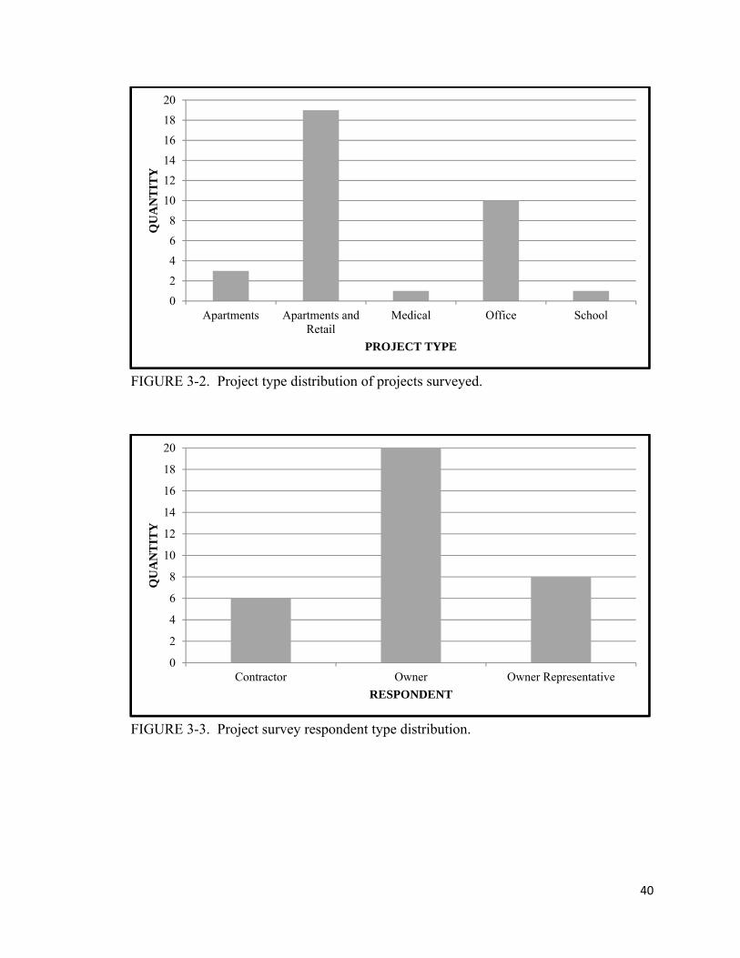
Of the 34 surveyed projects (including the two yet to be built), 19 of them were
apartments/retail, three of them were strictly apartments, one was a medical building, 10
of them were office buildings, and one was a school. This is outlined in Figure 3-2. The
respondents included six contractors, 20 owners, and eight owner representatives. This
information is shown in Figure 3-3.
40
FIGURE 3-2. Project type distribution of projects surveyed.
FIGURE 3-3. Project survey respondent type distribution.
0
2
4
6
8
10
12
14
16
18
20
Apartments Apartments andRetail
Medical Office School
QU
AN
TIT
Y
PROJECT TYPE
0
2
4
6
8
10
12
14
16
18
20
Contractor Owner Owner Representative
QU
AN
TIT
Y
RESPONDENT

41
Processing Survey Responses
Once the surveys were completed and collected, the data was entered into a
spreadsheet. This spreadsheet allowed for the tally of data to determine the percentage of
each project’s cost that was spent on the three construction sectors of interest. The
projects surveyed were also plotted on a map to show the distribution of work in the city
and what areas of the city have higher percentages of required demolition, abatement, and
remediation.
The following formulas were used to determine the three sector’s costs as a
percentage of construction value:
o Demolition cost as a percentage of construction value = Demolition Value/ Total
Construction Value (including the value of remediation, demolition, and
abatement)
o Abatement cost as a percentage of construction value = Abatement Value/ Total
Construction Value (including the value of remediation, demolition, and
abatement)
o Remediation cost as a percentage of construction value = Remediation Value/
Total Construction Value (including the value of remediation, demolition, and
abatement)
Additional Information
Data was also obtained from the Seattle Department of Planning and
Development (DPD). Seattle maintains a website database with issued permit data from

42
the past five years. This data was filtered to identify the quantity and value of
commercial construction projects in Seattle between 2011 and 2013.
43
Chapter 4: Research Results
Results
Table 4-1 below outlines the survey results. Appendix E contains the calculations for the
numbers discussed below. Figure 4-4 shows the locations of the projects surveyed in the city of
Seattle.

44
TABLE 4-1. Costs in dollars and as a percentage of project construction value for asbestos abatement, soil remediation, and building demolition for Seattle commercial construction projects surveyed.
Contaminated Soil Building Demolition Asbestos Abatement
Project Construction
value Remediation
value
Remediation cost as a
percent of total
construction value
Demolition value
Demolition cost as a
percent of total
construction value
Abatement value
Abatement cost as a
percent of total
construction value
A $ 47,176,370 Data not available $195,775 0.41% $9,826 0.02% B $ 13,263,258 $52,700 0.40% $222,800 1.67% $25,632 0.19% C $ 37,000,000 $75,000 0.20% $150,000 0.41% $50,000 0.14% D $ 14,250,000 $6,268 0.04% $69,300 0.49% $8,024 0.06% E $ 60,000,000 $215,000 0.36% $68,000 0.11% $0 0.00% F $ 11,212,528 $63,058 0.56% $52,000 0.46% $17,898 0.16% G $ 15,620,000 $87,958 0.56% $52,000 0.33% $34,230 0.22% H $ 9,322,441 $0 0.00% $68,480 0.73% $10,400 0.11% I $ 40,650,000 $85,000 0.21% $75,000 0.18% $2,000 0.00% J $ 61,325,000 $900,246 1.45% $18,000 0.03% $0 0.00%
K* $ 57,750,005 $1,246,478 2.10% $696,262 1.17% $259,000 0.44% L $ 46,000,000 $1,100,000 2.39% $600,000 1.30% $28,000 0.06% M $ 26,400,000 $175,000 0.66% $76,000 0.29% $15,000 0.06% N $ 6,750,000 $35,000 0.52% $45,000 0.66% $11,000 0.16% O $ 21,000,000 $0 0.00% $0 0.00% $0 0.00%
P** $ 58,300,000 $291,000 0.50% $240,000 0.41% $0 0.00% Q $ 11,516,841 $77,520 0.67% $0 0.00% $0 0.00% R $ 40,000,000 $30,000 0.08% $25,000 0.06% $8,000 0.02% S $ 16,000,000 $30,000 0.19% $45,000 0.28% $5,000 0.03% T $ 22,300,000 $2,500,000 10.81% $200,000 0.87% $70,000 0.30% U $ 49,000,000 $1,000,000 2.04% $247,000 0.50% $30,000 0.06% V $ 11,062,348 $0 0.00% $51,000 0.46% $28,000 0.25% W $ 50,000,000 $270,000 0.54% $0 0.00% $0 0.00% X $ 36,024,150 $326,704 0.91% $66,500 0.18% $26,100 0.07%

45
Contaminated Soil Building Demolition Asbestos Abatement
Project Construction
value Remediation
value
Remediation cost as a
percent of total
construction value
Demolition value
Demolition cost as a
percent of total
construction value
Abatement value
Abatement cost as a
percent of total
construction value
Y $ 34,536,234 $13,149 0.04% $140,808 0.41% $28,864 0.08% Z $ 56,834,218 $2,678,639 4.50% $120,893 0.20% $63,335 0.11% 1 $124,580,772 $95,339 0.08% $127,604 0.10% $107,784 0.09% 2 $ 73,946,435 $350,185 0.47% $0 0.00% $62,229 0.08% 3 $ 93,622,607 $3,265 0.00% $101,639 0.11% $83,528 0.09% 4 $ 75,871,094 $0 0.00% $56,742 0.07% $90,124 0.12% 5 $ 75,463,743 $0 0.00% $149,330 0.20% $79,665 0.11% 6 $ 78,333,692 $5,162,544 6.18% $0 0.00% $49,205 0.06%
7*** $ 76,000,000 $1,300,000 1.71% $185,000 0.24% $35,000 0.05% 8*** $ 41,000,000 $250,000 0.61% $0 0.00% $0 0.00%
*This project required a permanent soil contaminate extraction system at a cost to the project of $520,289. These dollars were not figured in the percentage calculations. **This project required a permanent soil contaminate extraction system at a cost to the project of $250,000. These dollars were not figured in the percentage calculations. ***These projects have not been started yet. The data is not used in calculating percentages, however the information is provided to show how developers budget for these costs and how they are planned for in actual projects slated to start.
TABLE 4-1 (Cont.)

46
Contaminated Soil
In consideration of the 31 projects surveyed, the average contaminated soil cost
per project was $544,195 which on average made up 1.18 percent of the projects cost.
Project A was not completed at the time of the survey so its soil remediation costs were
not considered in the average figures. Project T contaminated soil remediation costs far
exceeded the average proportional percentage of overall project cost.
Project T was an apartment building that was built on a property of a former dry
cleaning business. This business also stored fuel and lubricants for its delivery vehicle
fleet. The soil and ground water was contaminated with petroleum hydrocarbons as well
PCE’s. Additionally, the site also contained three heating oil UST’s and one UST that
contained dry-cleaning solvent (Liu 2012). There were five projects that had no
contaminated soil.
The standard deviation of contaminated soil costs in the projects surveyed was
$1,095,141 and 2.26 percent. Figure 4-1 graphically shows the standard deviation of
contaminated soil remediation costs as a percentage of construction value in the projects
surveyed.

47
FIGURE 4-1. Standard deviation of contaminated soil remediation costs as a percentage of construction value for Seattle commercial construction projects surveyed.
Building Demolition
In consideration of the 32 projects surveyed, the average building demolition cost
per project was $123,754 which on average made up 0.38 percent of the projects cost.
There were five projects that had no building demolition costs. The standard deviation of
building demolition costs for the projects surveyed was $155,884 and 0.40 percent.
Figure 4-2 graphically shows the standard deviation of building demotion costs as a
percentage of construction value in the projects surveyed that required demolition.
0
2
4
6
8
10
12
14
16
18
20
22
24
‐8% ‐6% ‐4% ‐2% 0% 2% 4% 6% 8% 10%
NUMBER
OF PROJECTS
REMEDIATION COST (PERCENT)

48
FIGURE 4-2. Standard deviation of building demolition costs as a percentage of construction value for Seattle commercial construction projects surveyed.
Asbestos Abatement
In consideration of the 32 projects surveyed, the average asbestos abatement cost
per project was $37,589 which on average made up 0.10 percent of a project’s cost.
Project K asbestos abatement costs far exceeded both the average cost and the average
proportional percentage of overall project cost.
Project K was a mixed use apartment/retail/commercial project that was built at
the site of a former dry cleaning business. The site also contained office buildings and
warehouses. The reason this project had such high abatement costs was a result of a
former industrial laundry facility. This building had asbestos containing material in the
pipe insulation and gaskets, exterior siding, drywall, floor tile, mastic, and window putty.
Additionally, there were six projects that did not require asbestos abatement.
0
2
4
6
8
10
12
14
16
18
20
‐1.00% ‐0.50% 0.00% 0.50% 1.00% 1.50% 2.00%
NUMBER
OF PROJECTS
DEMOLITION COST (PERCENT)

49
The standard deviation of asbestos abatement costs in the projects surveyed was
$50,633 and 0.10 percent. Figure 4-3 graphically shows the standard deviation of
asbestos abatement in the buildings surveyed as a percentage of construction value.
FIGURE 4-3. Standard deviation of asbestos abatement costs as a percentage of construction value for Seattle commercial construction projects surveyed.
Analysis
Contaminated Soil
The projects located in the neighborhood of South Lake Union had the greatest
proportion of project costs spent on soil remediation. The South Lake Union
neighborhood is also referred to as the Cascade area in Figure 4-4. South Lake Union has
historically been the industrial area of the city of Seattle. The projects that required no
contaminated soil abatement were dispersed throughout the city including three in the
0
2
4
6
8
10
12
14
16
18
20
22
‐0.3% ‐0.2% ‐0.1% 0.0% 0.1% 0.2% 0.3% 0.4% 0.5%
NUMBER
OF PROJECTS
ABATEMENT COST (PERCENT)

50
South Lake Union neighborhood. This shows that the amount of contaminates depends
on the prior property use, and not necessarily the general location of the project.
The average percentage of 1.18 percent suggests that commercial construction
projects in Seattle can expect to spend this proportion of their construction value in soil
remediation. The standard deviation indicates that there is not a lot of variation from the
average. This means that the projects surveyed all had costs relatively close to the
average. The standard deviation of 2.26 percent suggests that these projects should carry
an additional contingency fund of 3.44 percent of the project’s construction contract
value to account for unexpected contaminate costs or the outlier scenarios where a
specific project exceeds the average proportional costs.
Figure 4-1 indicates that the costs are normally distributed which means that 68
percent of projects will have contaminated soil costs within one standard deviation of the
average; between 0.00 percent and 3.44 percent. Also, 95 percent of projects will have
costs within two standard deviations of the average; between 0.00 percent and 5.70
percent of a project’s construction contract value.
Building Demolition
The average percentage of 0.38 percent suggests that commercial construction
projects in Seattle can expect to spend this proportion of their construction value in
building demolition if their site has existing structures present. Projects K and L both had
the highest demolition cost and the highest proportion of construction value resulting
from building demolition. These projects were both on sites that exceeded an acre in size
and consisted of warehouses.

51
The standard deviation graph shown in Figure 4-2 indicates that the demolition
costs are normally distributed and that projects above and below the average were still
close to that average. This means that expected demolition costs of future commercial
construction jobs in the city of Seattle should be predictable based off of these figures.
Asbestos Abatement
The average asbestos abatement percentage of 0.10 percent suggests that
commercial construction projects in Seattle can expect to spend this proportion of their
construction value in abatement. There were six projects or 19 percent of the projects
surveyed that had no asbestos containing material present. Half of these six projects also
correlate to projects that had no prior structure on the building site. Like the standard
deviation of building demolition, the standard deviation of asbestos abatement was low at
0.12 percent. This means that using these figures to extrapolate future abatement costs is
a reliable indicator the expected value of a project’s abatement requirements.

52
FIGURE 4-4. Location of Seattle commercial construction projects surveyed. Note: Map adapted from Seattle City Clerk's Geographic Indexing Atlas (n.d.).

53
Chapter 5: Discussion
Conclusion
The Seattle construction project survey results indicate that there is a substantial
proportion of a project’s cost that is dedicated to dealing with contaminated soil,
asbestos, and building demolition. There were approximately 164 commercial building
permits issued in Seattle in 2013 at a value of approximately $2.6 Billion (City of Seattle
2014). As shown in Appendix E, if the average cost percentages from the survey are
extrapolated using the value of permits issued in Seattle in 2013, that would mean these
projects spent a combined $30,680,000 on soil remediation, $9,880,000 on building
demolition, and $2,600,000 on asbestos abatement.
It is hard to say what national GDP figures would look like if asbestos abatement,
soil remediation, and building demolition were removed. But based on spending trends
discussed in Chapter 2 and 2012 GDP figures from Table A-1, the US GDP in 2012 was
$16,245 Billion and the construction industry’s value added was $581.07 Billion. With
asbestos abatement spending at $3 Billion/year and soil abatement spending at $8
Billion/year, the national GDP would be reduced to $16,234 Billion and the construction
industry’s value added would reduce by 1.89 percent. These are not significant figures
when considered independently.
54
However, there are also many other sectors and work outside of the three
construction areas that were discussed in this thesis that also inflate GPD in a negative
connotation. Some examples are: oil spill cleanup, fighting crime, natural disaster
response, commuting, vehicular accidents, and war. All of these items are great for the
economy and sometimes necessary for civilization and business, but they do not enhance
the welfare of the country or the happiness of its citizens.
Upon its creation, GDP was intended to only measure products and services that
are bought or sold. It was not intended as a guiding light for a country and its policy
decisions. Society has changed since its inception and the standards of progress need to
change as well. The environmental and social implications of policy decisions are
significantly greater now, more than ever.
An Environmental Assessment or Environmental Impact Statement is required on
nearly every construction project in the United States. These reviews outline the
environmental impacts and repercussions of the planned project. So why would the
government not discern between positive dollars and negative dollars? There is a
difference between a dollar spent on cutting down old growth timber that leads to the
extinction of an animal, and a dollar spent cutting down rapidly renewable timber that
impacts no animals. The government should not count them as the same dollar spent.
This same logic holds true for the three construction sectors discussed in this
thesis. The dollars spent to correct or cleanup after past damages or extemporaneous
materials should not be held in the same regard as dollars spent on new items that benefit
society and the environment such as solar panels, wind farms, and the construction of a
new school.

55
This research challenges the use of GDP and it demonstrates the contribution that
negative sectors make to the United States GDP. It exemplifies the need for mainstream
economic indicator that considers the social and environmental costs of earning a dollar;
especially if the United States is going to lead the world towards a sustainable future.
Research Limitations
When analyzing the results of the study, certain methods and limitations need to
be considered in context. The data in this thesis would unlikely be transferable across US
cities. Seattle was a major industrial town during the 1800’s and early 1900’s. Because it
is a port town as well as its proximity to the Klondike gold rush, Seattle had many
industries that abused the environment, which now necessitates the soil remediation that
is common today. Some of these industries include saw mills, ship building, drycleaners,
and railroads.
There are many other ancillary soft costs associated with dealing with soil
remediation, asbestos abatement, and building demolition that are not considered in this
study. Some of these items include: consultant fees, treatment of construction dewatering,
legal costs, jurisdiction fees, permanent treatment systems and insurance. In concept,
these items should be included when assessing data for the impact of the three discussed
construction sectors on GDP. However, the author elected to not include them for several
reasons; rather only hard disposal costs were included in this study.
It would be very difficult to get accurate data since a lot of times; these soft costs
are comingled with other necessary functions pertaining to the construction project. Also,
soft costs associated with these sectors can be very difficult to comprehensively define.
Finally, the soft costs can vary greatly depending on the building use as well as the

56
cleanup level desired by the developer. Often times, the baseline cleanup levels governed
by the federal or state jurisdiction are exceeded based on the developers desire to have a
‘clean bill of health’ for their site.
There are demolition costs on a jobsite that should not be considered in this study
including utility infrastructure, pavements or slabs, foundations, vegetation or trees, and
landscape features such as fences or retaining walls. Sometimes these items get wrapped
up into a demolition contract, and sometimes they are separated and performed by
another type of contractor. When possible to identify, the author removed these types of
demolition from the data figures. The reason it was removed was because these items are
not relevant to the buildings service life and should not influence the proportion that the
demolition of buildings prior to their useful service life has on GDP.
Finally, the NAICS discussed in Chapter 2 is set up by the United States Census
Bureau; however, the classification of businesses is left up to the business itself. This
makes it very difficult to compare local data collected to national figures. For example,
Sector 56 is Waste Management and Remediation/Remediation and Other Waste
Management Services/Remediation Services. Asbestos abatement contractors most likely
would classify their business in this sector; however, if they do other work such as
demolition then they may classify their work in Sector 23 which is
Construction/Specialty Trade Contractors/Site Preparation Contractors.
Also, it is nearly impossible to determine which sector all the contaminated soil
costs are being allocated to. Some of the costs are likely carried by general contractors
and subcontractors in their contracts. Some examples of this would be their time for
dealing with contaminates, trucking costs, and employee personal protective equipment.

57
However, the disposal costs are usually paid for by the developer. Developers may be
classified under different sectors as well. They may use Sector 23 if they are a
developer/builder, or Sector 53 which is Real Estate and Rental and Leasing. Another
sector that developers may classify under is Sector 52 which is Finance and Insurance.
Recommendations
The regulations and policies of the past have put a large environmental and
financial burden on the construction industry today. What will be the burden that the
current industry puts on future generations? It is difficult to anticipate but let’s hope that
the lessons learned from asbestos abatement and soil remediation era allow industry and
regulatory leaders to garner a more comprehensive understanding before moving ahead
with new technologies. The easiest way of doing something is not always the most
sustainable solution. Building designs and materials must be holistically assessed to
anticipate the needs of future occupants. Modern society cannot continue with a
disposability mindset.
The author does not suggest that GDP should be eliminated nor should these three
construction areas be removed from GDP. It is a good measurement tool when viewed in
context. However, the policy makers should consider both GDP and other indictors when
faced with creating polices and making economic decisions.
Further research is necessary to gauge the impacts of these three sectors in other
major metropolitan areas. Negative sectors were defined by the author for the purpose of
this thesis, however, the United States and the world need to create a recognized
definition of negative economics along with welfare enhancing economics. Through this
definition, sustainable development goals can be defined and pursued. Along with

58
defining negative sectors, a national and world method for reporting and tracking these
sectors needs to be developed.
It should not be the country’s goal to maximize GDP because it does not consider
the social costs or environmental impacts (Costanza et al. 2014). The United States and
the world needs to shift mindsets and agree upon a measurement system that considers
other important factors in life such as: physical/mental health, standard of living,
education, life expectancy, civic engagement, and life satisfaction as well as factors that
are important to our planet including sustainability, pollution, and depletion of natural
resources.

59
APPENDICES
Appendix A: Yearly GDP Figures
TABLE A-1. Yearly United States Gross Domestic Product from 1929-2013 in dollars and the construction sector’s yearly value added to Gross Domestic Product from 1947-2012 in dollars and as a percent.
United States Total
United States Construction
Year
GDP (billion) in
current dollars
GDP (billion) in
chained 2009
dollars
Value added in billions of current dollars
Value added in billions of chained
2009 dollars
Construction GDP as a
percentage of Total
GDP 1929 $105 $1,056 D a t a n o t a v a i l a b l e 1930 $92 $966 D a t a n o t a v a i l a b l e 1931 $77 $904 D a t a n o t a v a i l a b l e 1932 $60 $788 D a t a n o t a v a i l a b l e 1933 $57 $778 D a t a n o t a v a i l a b l e 1934 $67 $861 D a t a n o t a v a i l a b l e 1935 $74 $938 D a t a n o t a v a i l a b l e 1936 $85 $1,060 D a t a n o t a v a i l a b l e 1937 $93 $1,114 D a t a n o t a v a i l a b l e 1938 $87 $1,077 D a t a n o t a v a i l a b l e 1939 $94 $1,163 D a t a n o t a v a i l a b l e 1940 $103 $1,265 D a t a n o t a v a i l a b l e 1941 $129 $1,489 D a t a n o t a v a i l a b l e 1942 $166 $1,770 D a t a n o t a v a i l a b l e 1943 $203 $2,072 D a t a n o t a v a i l a b l e 1944 $225 $2,238 D a t a n o t a v a i l a b l e 1945 $228 $2,216 D a t a n o t a v a i l a b l e 1946 $228 $1,959 D a t a n o t a v a i l a b l e 1947 $250 $1,938 $8.90 $68.98 3.56% 1948 $275 $2,018 $11.10 $81.53 4.04% 1949 $273 $2,007 $11.22 $82.56 4.11% 1950 $300 $2,182 $12.79 $92.92 4.26% 1951 $347 $2,358 $15.26 $103.56 4.39% 1952 $368 $2,454 $16.44 $109.72 4.47%

60
United States Total
United States Construction
Year
GDP (billion) in
current dollars
GDP (billion) in
chained 2009
dollars
Value added in billions of current dollars
Value added in billions of chained
2009 dollars
Construction GDP as a
percentage of Total
GDP 1953 $390 $2,569 $17.06 $112.45 4.38% 1954 $391 $2,554 $17.18 $112.19 4.39% 1955 $426 $2,736 $18.44 $118.38 4.33% 1956 $450 $2,795 $20.28 $125.93 4.51% 1957 $475 $2,854 $21.30 $127.98 4.49% 1958 $482 $2,833 $20.98 $123.31 4.35% 1959 $523 $3,028 $22.74 $131.76 4.35% 1960 $543 $3,106 $23.15 $132.32 4.26% 1961 $563 $3,185 $24.11 $136.31 4.28% 1962 $605 $3,380 $25.93 $144.86 4.29% 1963 $639 $3,527 $27.66 $152.78 4.33% 1964 $686 $3,731 $30.32 $164.93 4.42% 1965 $744 $3,973 $33.28 $177.79 4.48% 1966 $815 $4,235 $36.62 $190.28 4.49% 1967 $862 $4,351 $38.20 $192.91 4.43% 1968 $943 $4,565 $41.82 $202.53 4.44% 1969 $1,020 $4,708 $46.71 $215.60 4.58% 1970 $1,076 $4,718 $49.49 $217.02 4.60% 1971 $1,168 $4,873 $54.47 $227.31 4.66% 1972 $1,282 $5,129 $60.18 $240.66 4.69% 1973 $1,429 $5,418 $68.17 $258.56 4.77% 1974 $1,549 $5,390 $72.98 $253.99 4.71% 1975 $1,689 $5,380 $73.69 $234.71 4.36% 1976 $1,878 $5,669 $84.20 $254.23 4.48% 1977 $2,086 $5,931 $92.82 $263.88 4.45% 1978 $2,357 $6,260 $109.72 $291.47 4.66% 1979 $2,632 $6,459 $124.84 $306.37 4.74% 1980 $2,863 $6,443 $131.51 $296.03 4.59% 1981 $3,211 $6,611 $133.13 $274.09 4.15% 1982 $3,345 $6,484 $131.03 $254.00 3.92% 1983 $3,638 $6,785 $139.56 $260.27 3.84% 1984 $4,041 $7,277 $160.73 $289.48 3.98% 1985 $4,347 $7,586 $176.96 $308.82 4.07%
TABLE A-1 (Cont.)

61
United States Total
United States Construction
Year
GDP (billion) in
current dollars
GDP (billion) in
chained 2009
dollars
Value added in billions of current dollars
Value added in billions of chained
2009 dollars
Construction GDP as a
percentage of Total
GDP 1986 $4,590 $7,852 $197.18 $337.31 4.30% 1987 $4,870 $8,124 $210.09 $350.44 4.31% 1988 $5,253 $8,465 $226.46 $364.97 4.31% 1989 $5,658 $8,777 $238.58 $370.12 4.22% 1990 $5,980 $8,945 $243.56 $364.36 4.07% 1991 $6,174 $8,939 $228.76 $331.21 3.71% 1992 $6,539 $9,257 $233.17 $330.07 3.57% 1993 $6,879 $9,511 $250.37 $346.18 3.64% 1994 $7,309 $9,895 $277.24 $375.34 3.79% 1995 $7,664 $10,164 $294.22 $390.19 3.84% 1996 $8,100 $10,550 $320.88 $417.90 3.96% 1997 $8,609 $11,023 $340.70 $436.26 3.96% 1998 $9,089 $11,513 $380.46 $481.94 4.19% 1999 $9,666 $12,071 $418.60 $522.79 4.33% 2000 $10,290 $12,565 $462.55 $564.84 4.50% 2001 $10,625 $12,684 $488.16 $582.77 4.59% 2002 $10,980 $12,910 $494.98 $581.95 4.51% 2003 $11,512 $13,270 $527.21 $607.71 4.58% 2004 $12,277 $13,774 $587.64 $659.29 4.79% 2005 $13,095 $14,236 $654.20 $711.16 5.00% 2006 $13,858 $14,615 $698.34 $736.50 5.04% 2007 $14,480 $14,877 $715.12 $734.70 4.94% 2008 $14,720 $14,834 $653.44 $658.47 4.44% 2009 $14,418 $14,418 $577.64 $577.64 4.01% 2010 $14,958 $14,779 $539.06 $532.61 3.60% 2011 $15,534 $15,052 $546.08 $529.16 3.52% 2012 $16,245 $15,471 $581.07 $553.39 3.58% 2013 $16,803 $15,767 D a t a n o t a v a i l a b l e
Note: Data adapted from United States Department of Commerce: Bureau of Economic Analysis, GDP by Industry: 1947-1997 (2014),United States Department of Commerce: Bureau of Economic Analysis, GDP by Industry: 1997-2012 (2014), and United States Department of Commerce: Bureau of Economic Analysis, Current-Dollar and "Real" Gross Domestic Product (2014).
TABLE A-1 (Cont.)

62
TABLE A-2. Delta between current year and previous year Gross Domestic Product and the delta between current year and previous year of construction sector’s value added to Gross Domestic Product.
United States Total United States Construction
Year Dollars
(billions) Percent Dollars
(billions) Percent 1929 Not applicable Data not available 1930 -$12.40 -11.85% Data not available 1931 -$14.80 -16.05% Data not available 1932 -$17.90 -23.13% Data not available 1933 -$2.30 -3.87% Data not available 1934 $9.60 16.78% Data not available 1935 $7.50 11.23% Data not available 1936 $10.60 14.27% Data not available 1937 $8.10 9.54% Data not available 1938 -$5.60 -6.02% Data not available 1939 $6.10 6.98% Data not available 1940 $9.40 10.05% Data not available 1941 $26.50 25.75% Data not available 1942 $36.60 28.28% Data not available 1943 $37.10 22.35% Data not available 1944 $21.50 10.59% Data not available 1945 $3.60 1.60% Data not available 1946 -$0.40 -0.18% Data not available 1947 $22.10 9.70% Not applicable 1948 $24.90 9.96% $2.21 24.80% 1949 -$2.00 -0.73% $0.12 1.08% 1950 $27.40 10.04% $1.56 13.93% 1951 $47.10 15.69% $2.47 19.32% 1952 $20.40 5.87% $1.19 7.78% 1953 $22.00 5.98% $0.62 3.75% 1954 $1.40 0.36% $0.12 0.69% 1955 $35.10 8.97% $1.26 7.34% 1956 $23.90 5.61% $1.84 10.00% 1957 $24.80 5.51% $1.02 5.02% 1958 $7.10 1.50% -$0.32 -1.49% 1959 $40.50 8.40% $1.75 8.35% 1960 $20.80 3.98% $0.41 1.81% 1961 $20.00 3.68% $0.96 4.15% 1962 $41.80 7.42% $1.83 7.58%

63
United States Total United States Construction
Year Dollars
(billions) Percent Dollars
(billions) Percent 1963 $33.50 5.54% $1.73 6.66% 1964 $47.20 7.39% $2.66 9.61% 1965 $57.90 8.44% $2.96 9.77% 1966 $71.30 9.59% $3.34 10.03% 1967 $46. 70 5.73% $1.59 4.33% 1968 $80.80 9.38% $3.61 9.46% 1969 $77.40 8.21% $4.89 11.69% 1970 $56.00 5.49% $2.79 5.97% 1971 $91.90 8.54% $4.98 10.06% 1972 $114.60 9.81% $5.70 10.47% 1973 $146.10 11.39% $7.99 13.28% 1974 $120.30 8.42% $4.81 7.06% 1975 $140.10 9.05% $0.71 0.97% 1976 $188.70 11.17% $10.51 14.26% 1977 $208.40 11.10% $8.62 10.24% 1978 $270.60 12.97% $16.90 18.21% 1979 $275.50 11.69% $15.13 13.79% 1980 $230.40 8.75% $6.67 5.34% 1981 $348.40 12.17% $1.62 1.23% 1982 $134.10 4.18% -$2.10 -1.58% 1983 $293.10 8.76% $8.53 6.51% 1984 $402.60 11.07% $21.17 15.17% 1985 $306.00 7.57% $16.23 10.10% 1986 $243.40 5.60% $20.22 11.43% 1987 $280.10 6.10% $12.90 6.54% 1988 $382.40 7.85% $16.37 7.79% 1989 $405.10 7.71% $12.12 5.35% 1990 $321.90 5.69% $4.98 2.09% 1991 $194.40 3.25% -$14.79 -6.07% 1992 $365.30 5.92% $4.41 1.93% 1993 $339.40 5.19% $17.20 7.38% 1994 $430.00 6.25% $26.87 10.73% 1995 $355.30 4.86% $16.98 6.12% 1996 $436.20 5.69% $26.65 9.06% 1997 $508.30 6.28% $19.83 6.18% 1998 $480.60 5.58% $39.76 11.67%
TABLE A-2 (Cont.)

64
United States Total United States Construction
Year Dollars
(billions) Percent Dollars
(billions) Percent 1999 $576.60 6.34% $38.15 10.03% 2000 $624.00 6.46% $43.95 10.50% 2001 $335.60 3.26% $25.61 5.54% 2002 $354.90 3.34% $6.81 1.40% 2003 $532.00 4.85% $32.23 6.51% 2004 $764.80 6.64% $60.43 11.46% 2005 $818.40 6.67% $66.56 11.33% 2006 $762.50 5.82% $44.14 6.75% 2007 $622.40 4.49% $16.78 2.40% 2008 $240.00 1.66% -$61.68 -8.63% 2009 -$302.40 -2.05% -$75.80 -11.60% 2010 $540.40 3.75% -$38.58 -6.68% 2011 $575.50 3.85% $7.02 1.30% 2012 $710.80 4.58% $34.99 6.41% 2013 $558.40 3.44% Data not available
Note: Data adapted from United States Department of Commerce: Bureau of Economic Analysis, GDP by Industry: 1947-1997 (2014),United States Department of Commerce: Bureau of Economic Analysis, GDP by Industry: 1997-2012 (2014), and United States Department of Commerce: Bureau of Economic Analysis, Current-Dollar and "Real" Gross Domestic Product (2014).
TABLE A-2 (Cont)

65
Appendix B: 2008-2009 NAICS Sector Earnings Variance
TABLE B-1. Delta between 2008 and 2009 value added to Gross Domestic Product organized by North American Industry Classification System (NAICS) sector code.
Sector Industry Title 2008 2009 Dollar
Variance Percent
Variance 11 Agriculture, forestry, fishing,
and hunting $154.6 $137.7 -$16.9 -10.9%
21 Mining $401.8 $291.0 -$110.8 -27.6% 22 Utilities $240.1 $253.7 $13.7 5.7% 23 Construction $653.4 $577.6 -$75.8 -11.6%
31-33 Manufacturing $1,807.7 $1,718.6 -$89.1 -4.9% 42 Wholesale trade $878.5 $823.5 -$55.1 -6.3%
44-45 Retail trade $857.8 $843.8 -$14.0 -1.6% 48-49 Transportation and
warehousing $423.5 $400.0 -$23.4 -5.5%
51 Information $727.1 $701.5 -$25.7 -3.5% 52 Finance and insurance $909.0 $970.8 $61.8 6.8% 53 Real estate and rental and
leasing $1,897.0 $1,904.5 $7.5 0.4%
54 Professional, scientific, and technical services
$1,052.5 $999.2 -$53.3 -5.1%
55 Management of companies and enterprises
$262.0 $247.7 -$14.4 -5.5%
56 Administrative and waste management services
$438.6 $414.0 -$24.6 -5.6%
61 Educational services $149.8 $163.5 $13.7 9.2% 62 Health care and social
assistance $997.4 $1,052.3 $54.9 5.5%
71 Arts, entertainment, and recreation
$139.9 $138.5 -$1.4 -1.0%
72 Accommodation and food services
$395.7 $384.2 -$11.5 -2.9%
81 Other services, except government
$331.4 $330.0 -$1.4 -0.4%
92 Public Administration $2,002.4 $2,065.8 $63.3 3.2% Note: Data adapted from United States Department of Commerce: Bureau of Economic Analysis, GDP by Industry: 1997-2012 (2014).

66
Appendix C: Survey Form

67
Project Survey of Asbestos Abatement, Soil Remediation, and Building Demolition Costs
Background: Gross Domestic Product (GDP) was first introduced during World War II by Simon Kuznets,
as a way to measure the United States’ wartime production of products and services. United States
construction contributed $520.3 billion (or 3.4% of the nation’s GDP) to the total 2011 GDP of $15,094
billion. This figure is skewed by commercial construction sectors (asbestos abatement, soil remediation,
and building demolition) that do not necessarily enhance the progress of the country, but rather correct
past policy and industry deficiencies. While these deficiencies have spurred the creation of construction
sectors to service the cleanup, they are tangential to the actual construction of commercial buildings.
Purpose: The purpose of this survey is to generate real industry data about the actual costs of asbestos
abatement, soil remediation, and building demolition relative to a project’s construction value in the city
of Seattle. This data will be used to compile my thesis report on Construction Sectors that Skew GDP.
About Me: My name is Jeff Christianson and I am a Superintendent at Exxel Pacific, Inc. I earned my BS
in Construction Management from Washington State University and am currently pursuing my MS in
Civil Engineering through the University of Maryland.
Notes:
1) It is preferable that projects also be included that entailed less (or even none) of the 3 items addressed
above. This will provide a truer barometer of the actual impacts these sectors may or may not have on
total project cost.
2) Please note if any of this information is confidential and I will not provide specifics in the paper with
regards to project location/name.
3) I am only looking for actual hard costs of the work performed. Please do not include soft costs such as
taxes, reports, 3rd party consultants, management time, permits, etc.
4) I can be reached [email protected] or 360‐815‐0724
Survey:
General Information
Name and Email :_______________________________________________________________________
Company:_____________________________________________________________________________
Project Name:_________________________________________________________________________
Project Address:________________________________________________________________________
Construction Start Date (mo/yr):__________________________________________________________
Construction Contract Value:_____________________________________________________________
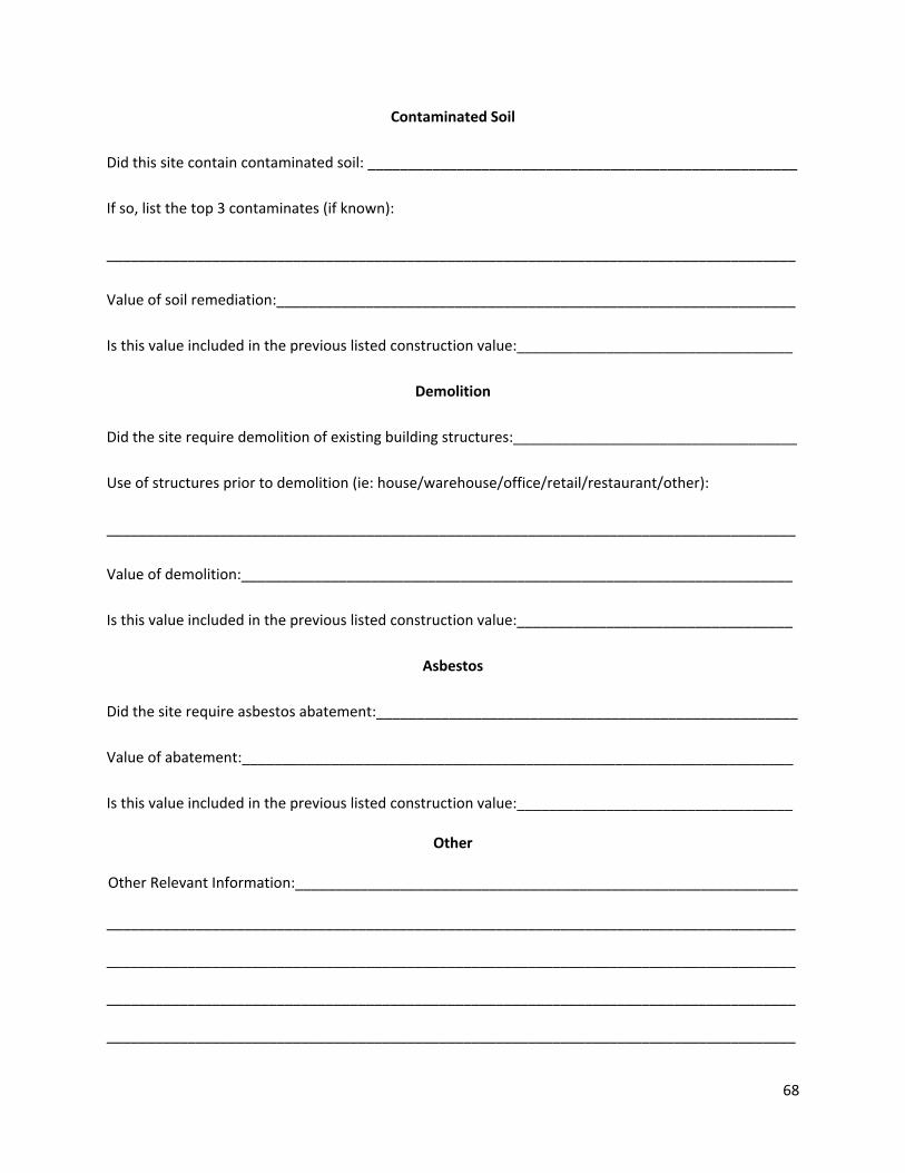
68
Contaminated Soil
Did this site contain contaminated soil: _____________________________________________________
If so, list the top 3 contaminates (if known):
_____________________________________________________________________________________
Value of soil remediation:________________________________________________________________
Is this value included in the previous listed construction value:__________________________________
Demolition
Did the site require demolition of existing building structures:___________________________________
Use of structures prior to demolition (ie: house/warehouse/office/retail/restaurant/other):
_____________________________________________________________________________________
Value of demolition:____________________________________________________________________
Is this value included in the previous listed construction value:__________________________________
Asbestos
Did the site require asbestos abatement:____________________________________________________
Value of abatement:____________________________________________________________________
Is this value included in the previous listed construction value:__________________________________
Other
Other Relevant Information:______________________________________________________________
_____________________________________________________________________________________
_____________________________________________________________________________________
_____________________________________________________________________________________
_____________________________________________________________________________________

69
Appendix D: Additional Survey Project Information
TABLE D-1. Project start date and building type for projects surveyed.
Project Project Start Date Building Product Type A Jan-14 Apartments and Retail B Sep-12 Apartments and Retail C May-10 Apartments and Retail D May-13 Apartments and Retail E Sep-12 Apartments and Retail F Feb-13 Apartments and Retail G Feb-13 Apartments and Retail H Jun-11 Office I Aug-09 Apartments and Retail J Feb-13 Office K Mar-12 Apartments and Retail L Jul-13 Apartments and Retail M Nov-10 Apartments and Retail N Dec-11 Apartments and Retail O Nov-07 Apartments and Retail P Nov-12 Apartments and Retail Q Oct-13 School R May-11 Apartments and Retail S Nov-11 Apartments and Retail T Jul-07 Apartments and Retail U Jun-08 Apartments and Retail V Jun-11 Apartments W Feb-12 Apartments X Aug-08 Office Y 2009 Office Z 2009 Office 1 2010 Office 2 2011 Office 3 2013 Office 4 2013 Office 5 2013 Office 6 2013 Medical 7 May-14 Apartments and Retail 8 Nov-14 Apartments

70
Appendix E: Survey Data Calculations
Contaminated Soil Remediation
Average cost (dollars):
x̅ = $52,700+$75,000+$6,268+$215,000+$63,058+$87,958+$0+$85,000+$900,246+
$1,246,478+$1,100,000+$175,000+$35,000+$0+$291,000+$77,520+$30,000+$30,000
$2,500,000+$1,000,000+$0+$270,000+$326,704+$13,149+$2,678,639+$95,339+
$350,185+$3,265+$0+$0+$5,162,544) / 31
x̅ = $544,195
Average (percent) of project construction value:
x̅ = (0.40%+0.20%+0.04%+0.36%+0.56%+0.56%+0.00%+0.21%+1.45%+2.10%+
2.39%+0.66%+0.52%+0.00%+0.50%+0.67%+0.08%+0.19%+10.81%+2.04%+0.00%+
0.54%+0.91%+0.04%+4.50%+0.08%+0.47%+0.00%+0.00%+0.00%+6.18%) / 31
x̅ = 1.18%
Standard Deviation of Cost (dollars):
σ = √ ((($52,700-$544,195)2+($75,000-$544,195)2+($6,268-$544,195)2+($215,000-
$544,195)2+($63,058-$544,195)2+($87,958-$544,195)2+($0-$544,195)2+($85,000-
$544,195)2+($900,246-$544,195)2+($1,246,478-$544,195)2+($1,100,000-$544,195)2
+($175,2000-$544,195)2+($35,000-$544,195)2+($0-$544,195)2+($291,000-$544,195)2
+($77,520-$544,195)2+($30,000-$544,195)2+($30,000-$544,195)2+($2,500,000-
$544,195)2+($1,000,000-$544,195)2+($0-$544,195)2+($270,000-$544,195)2+($326,704-
$544,195) 2+($13,149-$544,195)2 +($2,678,639-$544,195)2+($95,339-$544,195)2
+($350,185-$544,195)2+($3,265-$544,195)2+($0-$544,195)2+($0-$544,195)2+
($5,162,544-$544,195)2) / 31)
σ = $1,095,141

71
Standard Deviation (percent) of construction value:
σ = √ (((0.40%-1.18%)2+(0.20%-1.18%)2+(0.04%-1.18%)2+(0.36%-1.18%)2+(0.56%-
1.18%)2++(0.56%-1.18%)2+(0.00%-1.18%)2+(0.21%-1.18%)2+(1.45%-1.18%)2+(2.10%-
1.18%)2+(2.39%-1.18%)2+(0.66%-1.18%)2+(0.52%-1.18%)2+(0.00%-1.18%)2+(0.50%-
1.18%)2+(0.67%-1.18%)2+(0.08%-1.18%)2+(0.19%-1.18%)2+(10.81%-1.18%)2+(2.04%-
1.18%)2+(0.00%-1.18%)2+(0.54%-1.18%)2+(0.91%-1.18%)2+(0.04%-1.18%)2+(4.50%-
1.18%)2+(0.08%-1.18%)2+(0.47%-1.18%)2+(0.00%-1.18%)2+(0.00%-1.18%)2+(0.00%-
1.18%)2+(6.18%-1.18%)2) / 31)
σ = 2.26%
Building Demolition
Average Cost (dollars):
x̅ = ($195,775+$222,800+$150,000+$69,300+$68,000+$52,000+$52,000+$68,480+
$75,000+$18,000+$696,262+$600,000+$76,000+$45,000+$0+$240,000+$0+$25,000+
$45,000+$200,000+$247,000+$51,000+$0+$66,500+$140,808+$120,893+$127,604+$0
+$101,639+$56,742+$149,330+$0) / 32
x̅ = $123,754
Average (percent) of project construction value:
x̅ = (0.41%+1.67%+0.41%+0.49%+0.11%+0.46%+0.33%+0.73%+0.18%+0.03%+1.17%
+1.30%+0.29%+0.66%+0.00%+0.41%+0.00%+0.06%+0.28%+0.87%+0.50%+0.46%+
0.00%+0.18%+0.41%+0.20%+0.10%+0.00%+0.11%+0.07%+0.20%+0.00%) / 32
x̅ = 0.38%
Standard Deviation of Cost (dollars):
σ = √ ((($195,775-$123,754)2+($222,800-$123,754)2+($150,000-$123,754)2+($69,300-
$123,754)2+($68,000-$123,754)2+($52,000-$123,754)2+($52,000-$123,754)2+($68,480-

72
$123,754)2+($75,000-$123,754)2+($18,000-$123,754)2+($696,262-$123,754)2+
($600,000-$123,754)2+($76,000-$123,754)2+($45,000-$123,754)2+($0-$123,754)2+
($240,000-$123,754)2+($0-$123,754)2+($25,000-$123,754)2+($45,000-$123,754)2+
($200,000-$123,754)2+($247,000-$123,754)2+($51,000-$123,754)2+($0-$123,754)2+
($66,500-$123,754)2 +($140,808-$123,754)2+($120,893-$123,754)2+($127,604-
$123,754)2+($0-$123,754)2+($101,639-$123,754)2+($56,742-$123,754)2+($149,330-
$123,754)2+($0-$123,754)2) / 32)
σ = $155,884
Standard Deviation (percent) of construction value:
σ = √ (((0.41%-0.38%)2+(1.67%-0.38%)2+(0.41%-0.38%)2+(0.49%-0.38%)2+(0.11%-
0.38%)2+(0.46%-0.38%)2+(0.33%-0.38%)2+(0.73%-0.38%)2+(0.18%-0.38%)2+(0.03%-
0.38%)2+(1.17%-0.38%)2+(1.30%-0.38%)2+(0.29%-0.38%)2+(0.66%-0.38%)2+(0.00%-
0.38%)2+(0.41%-0.38%)2+(0.00%-0.38%)2+(0.06%-0.38%)2+(0.28%-0.38%)2+(0.87%-
0.38%)2+(0.50%-0.38%)2+(0.46%-0.38%)2+(0.00%-0.38%)2+(0.18%-0.38%)2+(0.41%-
0.38%)2+(0.20%-0.38%)2+(0.10%-0.38%)2+(0.00%-0.38%)2+(0.11%-0.38%)2+(0.07%-
0.38%)2+(0.20%-0.38%)2+(0.00%-0.38%)2) / 32)
σ = 0.40%
Asbestos Abatement
Average Cost (dollars):
x̅ = ($9,826+$25,632+$50,000+$8,024+$0+$17,898+$34,230+$10,400+$2,000+ $0+
$259,000+$28,000+$15,000+$11,000+$0+$0+$0+$8,000+$5,000+$70,000+$30,000+
$28,000+$0+$26,100+$28,864+$63,335+$107,784+$62,229+$83,528+$90,124+$79,665
+$49,205) / 32
x̅ = $37,589

73
Average (percent) of project construction value:
x̅ = (0.02%+0.19%+0.14%+0.06%+0.00%+0.16%+0.22%+0.11%+0.00%+0.00%+0.44%
+0.06%+0.06%+0.16%+0.00%+0.00%+0.00%+0.02%+0.03%+0.30%+0.06%+0.25%+
0.00%+0.07%+0.08%+0.11%+0.09%+0.08%+0.09%+0.12%+0.11%+0.06%) / 32
x̅ = 0.10%
Standard Deviation of Cost (dollars):
σ = √ ((($9,826-$40,433)2+($25,632-$40,433)2+($50,000-$40,433)2+($8,024-$40,433)2+
($0-$40,433)2+($17,898-$40,433)2+($34,230-$40,433)2+($10,400-$40,433)2+($2,000-
$40,433)2+($0-$40,433)2+($259,000-$40,433)2 +($28,000-$40,433)2+($15,000-$40,433)2
+($11,000-$40,433)2+($0-$40,433)2 +($0-$40,433)2+($0-$40,433)2+($8,000-$40,433)2+
($5,000-$40,433)2+ ($70,000-$40,433)2+($30,000-$40,433)2+($28,000-$40,433)2+($0-
$40,433)2 +($26,100-$40,433)2 +($28,864-$40,433)2+($63,335-$40,433)2+($107,784-
$40,433)2+ ($62,229-$40,433)2+($83,528-$40,433)2+($90,124-$40,433)2+($79,665-
$40,433)2+($49,205-$40,433)2) / 32)
σ = $50,633
Standard Deviation (percent) of construction value:
σ = √ (((0.02%-0.10%)2+(0.19%-0.10%)2+(0.14%-0.10%)2+(0.06%-0.10%)2+(0.00%-
0.10%)2+(0.16%-0.10%)2+(0.22%-0.10%)2+(0.11%-0.10%)2+(0.00%-0.10%)2+(0.00%-
0.10%)2+(0.44%-0.10%)2+(0.06%-0.10%)2+(0.06%-0.10%)2+(0.16%-0.10%)2+(0.00%-
0.10%)2+(0.00%-0.10%)2+(0.00%-0.10%)2+(0.02%-0.10%)2+(0.03%-0.10%)2+(0.30%-
0.10%)2+(0.06%-0.10%)2+(0.25%-0.10%)2+(0.00%-0.10%)2+(0.07%-0.10%)2+(0.08%-
0.10%)2+(0.11%-0.10%)2+(0.09%-0.10%)2+(0.08%-0.10%)2+(0.09%-0.10%)2+(0.12%-
0.10%)2+(0.11%-0.10%)2+(0.06%-0.10%)2) / 32)
σ = 0.10%
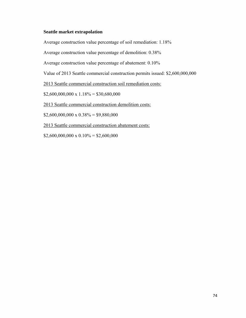
74
Seattle market extrapolation
Average construction value percentage of soil remediation: 1.18%
Average construction value percentage of demolition: 0.38%
Average construction value percentage of abatement: 0.10%
Value of 2013 Seattle commercial construction permits issued: $2,600,000,000
2013 Seattle commercial construction soil remediation costs:
$2,600,000,000 x 1.18% = $30,680,000
2013 Seattle commercial construction demolition costs:
$2,600,000,000 x 0.38% = $9,880,000
2013 Seattle commercial construction abatement costs:
$2,600,000,000 x 0.10% = $2,600,000

75
REFERENCES
About OSHA, WISHA, and DOSH. (n.d.). Washington State Department of Labor and
Industries. Retrieved February 15, 2014 from
http://www.lni.wa.gov/Safety/Basics/About/Default.asp
APA Formatting and Style Guide. (2014). Purdue University Online Writing Lab.
Retrieved February 25, 2014 from
https://owl.english.purdue.edu/owl/section/2/10/
Asbestos Abatement Contractors Receiving Certification from L&I. (n.d.). Washington
State Department of Labor and Industries. Retrieved February 21, 2014 from
http://www.lni.wa.gov/Safety/Topics/AtoZ/Asbestos/contractorlist.asp
Asbestos in the Home (n.d.). United States Consumer Product Safety Commission.
Retrieved from http://www.cpsc.gov/en/Safety-Education/Safety-
Guides/Home/Asbestos-In-The-Home/
Block, R., Herwijnen, F.V., Kozlowski, A., & Wolinski, S. (n.d.). Service Life and Life
Cycle of Building Structures. Retrieved from
http://www.dec.uc.pt/~luisss/cost/seminar/artics/service.pdf
Bukszpan, Daniel. (2012, June 01). Industries Hit Hardest by the Recession. Retrieved
from http://www.cnbc.com/id/47634901
76
Cauchon, Dennis. (1999, February 11). When Removing Asbestos Makes No Sense.
USA Today. Retrieved from http://www.nofluoride.com/asbestos.cfm
City of Seattle. (2014). Building permits issued in the past five years or currently in
progress. Retrieved February 06, 2014 from
https://data.seattle.gov/Permitting/Building-Permits-Current/mags-97de.
Cold War. (n.d.). Wikipedia. Retrieved February 01, 2014 from
http://en.wikipedia.org/wiki/Cold_War
Costanza, R., Kubiszewski, I., Giovannini, E., Lovins, H., McGlade, J., Pickett, K.,
Ragnarsdottir, K., Roberts, D., DeVogli, R., and Wilkinson, R. (2014). Time to
Leave GDP Behind. Nature, 505, 283-285.
Cui, Q., Johnson, P.W., and Sees, E. (2008). Long-Term Warranties on Highway
Projects. Tuscaloosa, Alabama: University Transportation Center of Alabama:
The University of Alabama.
Domitrovic, Brian. (2012, March 06). The Weak Dollar Caused the Great Recession.
Forbes. Retrieved from http://www.forbes.com/sites/briandomitrovic/
2012/03/13/the-weak-dollar-caused- the-great-recession/
Economic Census. (n.d.). United States Census Bureau. Retrieved February 02, 2014
from http://www.census.gov/econ/overview/index.html#construction
Fioramonti, Lorenzo. (2013). Gross Domestic Problem: The Politics Behind the World’s
Most Powerful Number. New York, NY: Zed Books.
Grebler, L., & Burns, L. S. (1982). Construction Cycles in the United States Since
World War II*. Real Estate Economics, 10(2), 123-151. doi: 10.1111/1540-
6229.00260

77
Gross National Happiness. (2014). Retrieved March 1, 2014 from
http://www.grossnationalhappiness.com/articles/
History of Asbestos Use. (2014). Mesothelioma Cancer Alliance. Retrieved February
15, 2014 from http://www.mesothelioma.com/asbestos-cancer/asbestos-
history.htm
Infoplease. (2005). Federal Minimum Wage Rates, 1955–2013. Retrieved February 14,
2014 from http://www.infoplease.com/ipa/A0774473.html
Institute for Economics and Peace. (2011). Economic Consequences of War on the U.S.
Economy. Retrieved from http://www.thereformedbroker.com/wp-
content/uploads/2012/02/Economic-Consequences-of-War.pdf
Koba, Mark. (2011, July 21). Recession: CNBC Explains. Retrieved from
http://www.cnbc.com/id/43563081
Landefeld, S., Seskin, E., and Fraumeni, B. (2008). Taking the Pulse of the Economy:
Measuring GDP. Journal of Economic Perspectives, 22 (2), 193-216. Retrieved
from http://www.bea.gov/about/pdf/jep_spring2008.pdf
Library of Economics and Liberty (2012). Wellbeing and Welfare. Retrieved from
http://www.econlib.org/library/Topics/College/wellbeingandwelfare.html
Liu, Jing. (2012, January 23). [No Further Action Letter]. Retrieved March 10, 2014
from https://fortress.wa.gov/ecy/gsp/CleanupSiteDocuments.aspx?csid=11514

78
O’Conner, Jennifer. (2004, October). Survey on Actual Service Lives for North
American Buildings. Paper presented at Woodframe Housing Durability and
Disaster Issues C, Las Vegas, United States. Paper retrieved from
http://www.woodworks.org/wp-content/uploads/2012/02/fpi-survey-actual-
service-lives.pdf
Robert Costanza Profile. (2013). In Australian National University: Crawford School of
Public Policy [Academic People page]. Retrieved February 07, 2014 from
https://crawford.anu.edu.au/people/academic/robert-costanza
Roose, Kenneth. (1948). The Recession of 1937-38. Journal of Political Economy,
56(3), 239-248. Retrieved from http://www.jstor.org/stable/1825772
Seasonal Adjustment of Chained Dollars. (n.d.). Retrieved February 07, 2014 from
https://www.census.gov/foreign-trade/aip/seasonalchain.html
Seattle City Clerk's Geographic Indexing Atlas. (n.d.). Retrieved February 08, 2013
from http://clerk.ci.seattle.wa.us/~public/nmaps/fullcit2.htm
Simon Kuznets: Facts. (2014). Nobel Prize. Retrieved January 31, 2014 from
http://www.nobelprize.org/nobel_prizes/economic-sciences/laureates/1971/
kuznets-facts.html
Slaying the Dragon of Debt: Fiscal Politics & Policy from the 1970s to the Present.
(2011). University of California, Berkley. Retrieved February 14, 2014 from
http://bancroft.berkeley.edu/ROHO/projects/debt/timeline.html
Stanton, Elizabeth A. (2007, February). The Human Development Index: A History.
Retrieved from http://scholarworks.umass.edu/peri_workingpapers/85/

79
Talberth, J., Cobb, C., Slattery, N. (2007, February). The Genuine Progress Indicator
2006: A Tool for Sustainable Development. Redefining Progress. Retrieved
from http://rprogress.org/publications/2007/GPI%202006.pdf
The Happy Planet Index. (2014). Retrieved March 1, 2014 from
http://www.happyplanetindex.org/about/ on
The Possible Course of the 1958 Recession. (1958). Progressive Calvinism, 4(5), 129-
134. Retrieved from http://www.contra-mundum.org/pc/PC4-05.pdf
United Nations: The Future We Want. (2012). The Future We Want. Retrieved from
http://www.uncsd2012.org/content/documents/727The%20Future%20We%20Wa
nt%2019%20June%201230pm.pdf
United States Department of Commerce: Bureau of Economic Analysis. (2014).
Current-Dollar and "Real" Gross Domestic Product. [Data file]. Retrieved from
www.bea.gov/national/xls/gdplev.xls
United States Department of Commerce: Bureau of Economic Analysis. (2014). GDP
by Industry: 1947-1997. [Data file]. Retrieved from
http://www.bea.gov/industry/xls/GDPbyInd_VA_NAICS_1947-1997.xls
United States Department of Commerce: Bureau of Economic Analysis. (2014). GDP
by Industry: 1997-2012. [Data file]. Retrieved from
http://www.bea.gov/industry/xls/GDPbyInd_VA_NAICS_1997-2012.xlsx
United States Department of Commerce: Bureau of Economic Analysis. (n.d.). Regional
Data. Retrieved from http://www.bea.gov/iTable/iTable.cfm?reqid=70&step=
1&isuri=1&acrdn=2#reqid=70&step=1&isuri=1

80
United States Department of Energy. (1994, February). A Comparison of the RCRA
Corrective Action and CERCLA Remedial Action Processes. Retrieved from
http://www.qe3c.com/dqo/project/level5/rcracomp.pdf
United States Department of Health and Human Services: National Toxicology Program.
(2011). Report on Carcinogens (12th ed.). Retrieved from
http://ntp.niehs.nih.gov/ntp/roc/twelfth/profiles/Asbestos.pdf
United States Department of Labor. (2009). Reflections on OSHA’s History. Retrieved
from https://www.osha.gov/history/OSHA_HISTORY_3360s.pdf
United States Department of Labor: Bureau of Labor Statistics. (2006, August 03). 100
Years of U.S. Consumer Spending: Data for the Nation, New York City, and
Boston. Retrieved from http://www.bls.gov/opub/uscs/
United States Department of Labor: Occupational Safety & Health Administration
[OSHA]. (n.d.). Regulations (Standard 1926.1101). Retrieved from
https://www.osha.gov/pls/oshaweb/owadisp.show_document?p_id=10862&p_tabl
e=STANDARDS
United States Environmental Protection Agency. (1997, May). Best Management
Practices for Soils Treatment Technology: Suggested Operational Guidelines to
Prevent Cross-Media Transfer of Contaminants During Cleanup Activities.
Retrieved from http://www.epa.gov/osw/hazard/correctiveaction/resources/
guidance/rem_eval/bmpfin.pdf
United States Environmental Protection Agency. (2004). Cleaning up the national waste
sites: Markets and Technology Trends (2004 Edition). Retrieved from www.clu-
in.org/download/market/2004market.pdf

81
United States Environmental Protection Agency. (2009). Estimating 2003 Building-
Related Construction and Demolition Material Amounts. Retrieved from
http://www.epa.gov/osw/conserve/imr/cdm/pubs/cd-meas.pdf
United States Environmental Protection Agency. (2012). RCRA Orientation Manual
2011: Resource Conservation and Recovery Act. Retrieved from
http://www.epa.gov/osw/inforesources/pubs/orientat/
United States Environmental Protection Agency. (2013). National Priorities List.
Retrieved February 22, 2014 from
http://www.epa.gov/superfund/sites/npl/index.htm
US Federal Bans on Asbestos (2013). United States Environmental Protection Agency.
Retrieved from http://www2.epa.gov/asbestos/us-federal-bans-asbestos
Washington State Department of Ecology. (2007, November). Model Toxics Control Act
Statute and Regulation. Retrieved from
https://fortress.wa.gov/ecy/publications/publications/9406.pdf
What are Asbestos Related Lung Diseases? (2011). National Heart, Lung and Blood
Institute. Retrieved February 15, 2014 from
http://www.nhlbi.nih.gov/health/health-topics/topics/asb/
World Values Association. (2012). 2010-2012 World Values Survey [Survey form].
Retrieved from http://www.worldvaluessurvey.org/wvs/articles/folder_
published/article_base_136/files/WVS_2010-2014_Questionnaire_v2012-06.pdf