ABSTRACT Title of Document: A SYSTEMS ENGINEERING ...austin/RecentGraduates/MSSE-Johnnie2011.pdf · A SYSTEMS ENGINEERING FRAMEWORK FOR METABOLIC ENGINEERING EXPERIMENTS By Joseph

ABSTRACT

Title of Document: A SYSTEMS ENGINEERING

FRAMEWORK FOR METABOLIC

ENGINEERING EXPERIMENTS

Joseph Johnnie, Master of Science in Systems

Engineering, 2011

Directed By: Dr. Mark Austin, Department of Civil and

Environmental Engineering, and the Institute

for Systems Research, University of Maryland

at College Park

Cells of living organisms simultaneously operate hundreds or thousands of

interconnected chemical reactions. Metabolic networks include these chemical reactions

and compounds participating in them. Metabolic engineering is a science centered on the

analysis and purposeful modification of an organism's metabolic network toward a

beneficial purpose, such as production of fuel or medicinal compounds in

microorganisms. Unfortunately, there are problems with the design and visualization of

modified metabolic networks due to lack of standardized and fully developed visual

modeling languages. The purposes of this paper are to propose a multilevel framework

for the synthesis, analysis and design of metabolic systems, and then explore the extent to

which abstractions from systems engineering (e.g., SysML) can complement and add

value to the abstractions currently under development within the greater biological

community (e.g., SBGN). The computational test-bed that accompanies this work is

production of the anti-malarial drug artemisinin in genetically engineered

Saccaharomyces cerevisiae (yeast).

A SYSTEMS ENGINEERING FRAMEWORK FOR METABOLIC ENGINEERING

EXPERIMENTS

By

Joseph Johnnie

Thesis submitted to the Faculty of the Graduate School of the

University of Maryland, College Park, in partial fulfillment

of the requirements for the degree of

Master of Science in Systems Engineering

2011

Advisory Committee:

Dr. Mark Austin, Chair

Dr. Ganesh Sriram, Committee Member

Dr. Ray Adomaitis, Committee Member

© Copyright by

Joseph Johnnie

2011

i

Dedication

This paper is dedicated to my parents, Elizabeth Johnnie and Johnnie Nedungattu.

Without their steadfast support, I would not be where I am today.

ii

Acknowledgements

I would like to acknowledge the following people, all of whom have contributed

to this work. Dr. Mark Austin (Department of Civil and Environmental Engineering and

Institute of Systems Research), in his role as thesis advisor, helped me to define the

overall scope and direction of my research. He has provided me technical advice with

respect to understanding metabolic engineering from a systems perspective, and editorial

input on my research papers as well. Assistant Professor Ganesh Sriram (Department of

Biomolecular and Chemical Engineering) has helped guide me through the metabolic

research for this paper. He has been instrumental in introducing and bringing me up to

speed in the metabolic engineering space to the point where I could successfully integrate

metabolic engineering with systems engineering. Professor Raymond Adomaitis brought

a unique perspective as a professor with dual faculty appointments in the departments of

Biomolecular and Chemical Engineering and the Institute for Systems Research. Since

this research aims to integrate research from these two fields, his input was invaluable.

Dr. Austin, Dr. Sriram, and Dr. Adomaitis all served as members of the thesis

committee with Dr. Austin functioning as chair.

Dr. Ashish Misra and Mr. Matt Conway, members of Dr. Sriram’s lab, were also

implementing Flux Balance Analysis for their own individual projects during the summer

of 2011. Rather than pursue these efforts separately, we decided to unite our efforts as a

group. This resulted in a lot of positive momentum which we each carried forward into

our own individual research. I am grateful to them for their help and assistance with the

metabolic engineering component of my research.

iii

Mrs. Susan Frazier, the Institute of Systems Research Director of Human

Resources and Education, was instrumental in encouraging me to pursue the research

based master’s degree in systems engineering and guiding me through the application

process. Without her help, I would have never had the opportunity to complete this

project.

I would also like to thank the Institute of Systems Research community as a

whole, along with the members of the Sriram Metabolic Engineering Laboratory. Both

groups fostered a tremendously supportive environment in which to pursue research.

iv

Table of Contents Dedication ................................................................................................................................... i

Acknowledgements ..................................................................................................................... ii

Table of Contents ....................................................................................................................... iv

List of Tables ............................................................................................................................. vi

List of Figures........................................................................................................................... vii

Chapter 1 Introduction ................................................................................................................ 1

1.1 - Problem Statement .......................................................................................................... 1

1.2 – Scope and Objectives...................................................................................................... 5

Chapter 2 – Multi-Level Framework for Orchestration of Good Design Solutions ....................... 7

2.1 – Approach........................................................................................................................ 7

2.1.1 - Strategies for Dealing with Increases in System Complexity ..................................... 7

2.1.2 - Solution Mechanisms ............................................................................................. 10

2.1.3 - Multi-Level Framework for Metabolic Process Design ........................................... 13

2.1.4 - Systems Integration ................................................................................................ 15

2.2 – Semi-Formal Models for Metabolic Engineering ........................................................... 16

2.2.1- Goals and Scenarios ................................................................................................ 16

2.2.2 – Abstraction: Ad Hoc Metabolic Engineering Diagrams .......................................... 17

2.2.3 - Abstractions: SBGN ............................................................................................... 18

2.2.4 - Abstractions: SysML .............................................................................................. 23

2.3 - Formal Models for Metabolic Engineering .................................................................... 27

2.3.1 - Flux Balance Analysis ............................................................................................ 27

2.3.2 - OPTKNOCK Algorithm ......................................................................................... 32

2.4 - Formal Model Interface Design for Systems Integration ................................................ 36

Chapter 3 – Metabolic Engineering Experiment ........................................................................ 38

3.1 – Background .................................................................................................................. 38

3.1.1 – Semi-formal Model Design - Goals ........................................................................ 38

3.1.2- Motivation and History ............................................................................................ 38

3.1.3 – Advance 1: CYP71AV1/CPR Pathway .................................................................. 39

3.1.4 – Advance 2: DBR2 Pathway .................................................................................... 41

3.2 - Formal Models for Metabolic Engineering .................................................................... 43

3.2.1 - Tools ...................................................................................................................... 43

v

3.2.2 - Methodology .......................................................................................................... 44

3.2.3 - Preparing the Model ............................................................................................... 46

3.2.4 - Setting Parameters and Constraints ......................................................................... 51

3.2.5 - OPTKNOCK Results and FBA Verification ................................................................. 53

3.3 – Semi-Formal Models for Metabolic Engineering ........................................................... 57

3.3.1 - Ad Hoc Abstraction ................................................................................................ 58

3.3.2 - SBGN Abstraction .................................................................................................. 61

3.3.3 - SysML Abstraction................................................................................................. 63

3.4 - Systems Integration for Metabolic Engineering ............................................................. 65

Chapter 4 – Conclusion ............................................................................................................. 69

4.1 - Summary ...................................................................................................................... 69

4.2 - Future Work .................................................................................................................. 70

References ................................................................................................................................ 72

Appendices ............................................................................................................................... 77

Appendix A – MATLAB code .............................................................................................. 77

vi

List of Tables

Table 1 - Features and problems of ad hoc graphical notations (Novere et al, 2009) ....... 19

Table 2 - Comparison between the three languages of SBGN (Novere et al, 2009)......... 21

Table 3 - Preparing the Yeast model – Strain 1 .............................................................. 49

Table 4 - Preparing the Yeast model - Strain 2 ............................................................... 51

Table 5 - Preparing the Yeast Model - Strain 3 .............................................................. 51

Table 6 - List of Target Reactions .................................................................................. 53

Table 7 - OPTKNOCK Results and Verification (Units: mol•gDW-1

• h-1

).................... 53

vii

List of Figures

Figure 1 - Complete Yeast Metabolism (Schellenberger et al, 2010); Highlighted areas

represent pathways of high metabolic traffic ....................................................................2

Figure 2 – Sources of complexity from a biological systems viewpoint ............................9

Figure 3 - Sources of complexity from a metabolic systems design viewpoint..................9

Figure 4 - Increases in programmer productivity over time (Austin 2011) ........................9

Figure 5 - A Multi-level framework for synthesis, analysis, design and integration of

models in metabolic system design. ............................................................................... 14

Figure 6 - Framework for integration of semi-formal models with formal models .......... 16

Figure 7 - Metabolic Engineering Diagrams (Yang et al, 2011; Boyle et al, 2011) ......... 17

Figure 8 - SBGN examples: (a) process diagram, (b) entity relationship diagram, (c)

SBGN activity flow diagram (Novere et al, 2009). ......................................................... 20

Figure 9 - SBGN Process diagram for Glycolysis .......................................................... 22

Figure 10 - Glyphs for SBGN Process Diagrams ........................................................... 22

Figure 11 - SysML Taxonomy (OMG: SysML v 1.2, 2010) ........................................... 24

Figure 12 - Internal Block Diagram of a Distiller (Friedenthal et al, 2009) .................... 25

Figure 13 - Parametric Diagram of a Distiller (Friedenthal et al, 2009) ......................... 26

Figure 14- How to translate a reaction network into a linear algebra expression with

stoichiometric matrix and flux vector. (Athanasiou et al, 2003) ...................................... 28

Figure 15 - Applying Steady State and solving for fluxes using linear algebra (Athanasiou

et al, 2003)..................................................................................................................... 29

Figure 16 - Flux balance analysis (Orth et al, 2010). ...................................................... 30

Figure 17 - If a linear program has a non-empty, bounded feasible region, the optimal

solution will always be one of the corner points (Arsham 2011). .................................... 31

Figure 18 - Flux Balance Analysis - Overall Approach (Orth et al, 2010) ...................... 32

Figure 19 - OPTKNOCK algorithm framework (Burgard et al, 2003) ........................... 33

Figure 20 - Bilevel programming framework - maximizing cellular and bioengineering

objectives (Burgard et al, 2003) .................................................................................... 34

Figure 21 – Venn Diagram showing common and distinct features of SysML and SBGN,

together with a framework for wrapping formal models with SysML interface constructs

(e.g., ports). ................................................................................................................... 36

Figure 22 - Schematic Representation of engineered artemisinic acid biosynthetic

pathway in S. cerevisiae (Ro et al, 2006) ....................................................................... 40

Figure 23 - Covello Group Pathway (Source: Zhang et al, 2008).................................... 42

Figure 24 - Schematic of a Computational Metabolic Engineering Experiment .............. 45

Figure 25 - A Bar Graph Comparing Pre and Post Knockout fluxes for each strain ........ 54

Figure 26 - Lysine Metabolic Pathway ........................................................................... 56

Figure 27 –A Non standard de facto Visual Abstraction generated using BIGG and the

COBRA Toolbox (Hyduke et al, 2011)) ......................................................................... 59

viii

Figure 28 – SBGN compliant notation, generated using VANTED and SBGN-ED

software (Junker et al, 2006; Czauderna et al, 2010).. ................................................... 60

Figure 29 - SysML Visual Model for Pathways of Interest The target pathway for flux is

highlighted and the suggested knockouts are crossed out. .............................................. 62

Figure 30 - Parametric Diagram defining parameters and constraints between MICITD

and HACNH reactions ................................................................................................... 63

Figure 31 - Systems Integration - Plugging the in silico metabolic engineering experiment

into the Systems Engineering framework ....................................................................... 67

1

Chapter 1 Introduction

1.1 - Problem Statement

Throughout the systems engineering community, a well-known tenet is that good

designs balance the need for functionality and performance against limitations on cost.

During the pre-implementation stages of system development (i.e., where a detailed

system description may not exist), systems engineers are concerned primarily with

system functionality and the identification of key environmental conditions within which

this functionality must occur. Models of functionality need to describe what the system

will do, and the order in which these functions will be executed, under both normal and

abnormal operating conditions. The answers to these basic concerns are commonly

expressed as functional requirements. Performance requirements describe how well a

system should perform these functions. Interface requirements describe conditions that

will allow for communication between subsystems, and, between subsystems and the

external environment. Then, as the system development proceeds, engineers assume that

it will be possible to control the complexity of developments through separation of design

concerns (e.g., function before implementation; logic and physical representations) and

decomposition of design solutions into hierarchies. Together these strategies of

development lead to loosely coupled system architectures and well-defined hierarchies of

behavior which, in turn, can facilitate the definition of simulation models (or

corresponding experimental test-beds) and procedures for efficient search of the design

space for solutions that are feasible (i.e., satisfy all constraints) and provide a desirable

tradeoff in design criteria.

2

Figure 1 - Complete Yeast Metabolism (Schellenberger et al, 2010); Highlighted areas represent pathways of high metabolic traffic

3

These principles apply to a wide range of established and emerging application

areas. As a case in point, metabolic networks are immensely complex systems

characterized by large numbers of nodes (chemical compounds, hereafter referred to as

metabolites), and interconnections (reactions). The metabolism of a single

microorganism such as Escherica coli or S. cerevisiae (yeast) is massive, composed of

thousands of metabolites and reactions regulated by hundreds of genes, which interact

with each other in a combinatorial fashion to maintain the cell’s living state (Figure 1).

Recent advances in computer technology and bioinformatics have allowed for

detailed analyses of these metabolic systems. Examples include the creation of

metabolic models for organisms such as E. coli and S. cerevisiae in languages such as

SBML (systems biology markup language), and the development of algorithms to

identify nontrivial bottleneck reactions in these models. However, due to a lack of

visual abstraction capabilities, procedures for the systematic and precise design (i.e.,

modification and construction) of metabolic networks are not as straightforward and

predictable as they should be. For example, while engineers have algorithms to process

a metabolic network and identify reactions of interest, the results are not automatically

carried through to visual diagrams showing where the reactions are located within the

overall metabolic system.

State-of-the-art metabolic engineering procedures apply an understanding of

reaction kinetics from chemical engineering to the chemical networks and compounds

of cells from the biological domain. Value in metabolic systems is generated by

maximizing production rate of a metabolite of interest or maximizing carbon flux

through its synthesis pathway, while minimizing energy cost associated with

4

compounds such as ATP (adenosine triphosphate) and NAD(P)H (Nicotinamide

adenine dinucleotide (phosphate)). Metabolic engineers identify and investigate how

specific modifications to the metabolic network (e.g., reaction knockouts or gene

overexpression) result in redirection of carbon traffic in the system as a whole.

Computational analysis and linear programming methods are used to simulate and

predict experimental results while genetic engineering is used to implement the design.

Unfortunately, this process requires extensive human input and is time consuming. One

source of inefficiency stems from less-than-perfect algorithms sometimes suggesting

reactions whose modifications result in cell death, or whose modifications are

impossible to implement through genetic engineering. This puts researchers in a

position where code may need to be rewritten multiple times before it outputs reaction

modifications that are experimentally feasible.

Overcoming these limitations will require new approaches to identifying and

handling design modifications such as reaction knockouts. Reaction knockouts are a

type of modification to a metabolic network in which a reaction is eliminated and a

pathway becomes a dead end. Since carbon cannot flow through an interrupted

pathway, the flux is often rerouted through other pathways in the metabolic network.

When applied strategically, reaction knockouts can reroute flux towards a targeted

pathway. However, reaction knockouts vary in impact, ranging from no effect on

reaction flux (e.g., if the knockout reaction is on a pathway in parallel with other paths)

to total reduction of all cellular flux to zero, also known as cell death (e.g., if a reaction

is in a main branch of the network). A second source of difficulty stems from the non-

additive nature of reaction knockouts. This occurs due to flux interactions. As a result,

5

design procedures based upon sequences of individual knockouts are sometimes less

than optimal. To overcome this barrier, design procedures need to handle combinations

of knockouts. When this fact is coupled with large network size, the complexity of the

design space explodes in combinatorial fashion. This results in an algorithm’s

application becoming much more computationally intensive and time consuming.

To see how the high degree of interconnectivity between biological nodes

creates combinatorial explosion, consider a 3 knockout experiment of 500 reactions.

This corresponds to nCr = 500C3 = 20,708,500 knockout combinations. If the designer

wanted to complete 3 knockouts on a higher-level organism with 900 reactions,

knockout combinations increase to nCr = 500C3 = 121,095,300. Increasing the number of

knockouts further to 6, gives nCr = 500C6 = 21,057,686,727,000 possibilities. This rapid

growth in possible combinations creates a gap between what is required from a system

perspective, and what is possible from a design and validation perspective. Smarter

approaches to computational metabolic engineering would incorporate knowledge of

dependencies among metabolites, and employ combinations of “system decomposition

and abstraction” to keep the complexities of metabolic computations in check.

1.2 – Scope and Objectives

When working with complex biological systems, metabolic engineers

continually seek new approaches to the synthesis, design, and assessment of system-

level architectures. For example, scientists have suggested that the biological

community needs to lay broad foundations with respect to the concepts of

standardization, decoupling and abstraction (Endy 2005). Still, many questions remain.

How, for example, can one design metabolic processes with less human intervention

6

and greater efficiency through automation? What kinds of design tools will work for

extremely large biological systems? We hypothesize that various forms of assistance

will be useful to the metabolic engineering and greater biological community.

Assistance can be provided in the form of design principles (e.g., rules of development)

and building blocks upon which good design solutions can be built. Designers also need

mechanisms to: (1)Dynamically control the levels of detail that will be presented to an

engineer, and (2)Dynamically reconfigure statements of system functionality in

response to the identification of designer mistakes and/or changes in required

functionality.

This thesis has two purposes. In Chapter 2, we propose a multi-level framework

for the synthesis, analysis and design of metabolic systems. This framework will

employ a variety of modeling abstractions, approaches to design specification, and

strategies for systems integration. In Chapter 3, we apply this framework to a metabolic

engineering experiment in which the objective is to optimize a yeast strain genetically

engineered to produce artemisninin via reaction knockouts. We will pay special

attention to semiformal models of visual abstraction and interfacing them with more

formal models of simulation. This is an area with strong precedents in systems

engineering, but limited development in the metabolic engineering space. In Chapter 4,

we will present a summary of the work and suggestions for future research. Scripts of

the MATLAB code for the in silico experiment can be found in Appendix A.

7

Chapter 2 – Multi-Level Framework for Orchestration of Good

Design Solutions

2.1 – Approach

Metabolic systems are complex heterogeneous systems developed by teams of

researchers, many of whom will have expertise in only one or two aspects of biology

(e.g., cell biology; functional genomics; genetics, microbiology, bioinformatics etc.).

To this end, and in support of the synthesis, design, integration, and evaluation of

metabolic systems, this chapter formulates a multi-level framework for the

orchestration of good design solutions. We expect that high levels of productivity will

be achieved through the use of high-level visual abstractions coupled with lower-level

(mathematical) abstractions suitable for formal systems analysis.

2.1.1 - Strategies for Dealing with Increases in System Complexity

From both a scientific and engineering perspective, metabolic networks are

immensely complex systems characterized by large numbers of nodes (chemical

compounds, hereafter referred to as metabolites), and interconnections (reactions).

History tells us that as technologies improve over time, scientists are provided with

better tools to conduct experimental observations and collect experimental data. This, in

turn, allows for the formulation of new hypotheses aimed at explaining the mechanisms

and dynamics behind experimental observations. After more than five decades of

modern biological research, we are now entering an era where mathematical modeling

of biological and biochemical systems can provide insight into the system structure

(e.g., organs, tissues, cells and molecules, connections among components) and system

behavior (e.g., detailed dynamics of biochemical interactions; built in control/defense

8

mechanisms to provide protection against environmental attack) (Tomlin 2005, Tomlin

2007).

From a systems engineering perspective, biologists are not designing and

creating more complicated systems per se - instead, they observe systems in the hope of

creating a better understanding of the architecture, behavior, and control mechanisms in

the biological system. The associated increase in observational complexity over time is

shown in Figure 2. We assume that in the beginning, scientific studies will lead to large

improvements in knowledge and understanding of the biological system, but that longer

term, further studies will produce diminishing returns.

One consequence of these advances is an ongoing desire to apply metabolic

engineering in higher level organisms, with each iteration of design and development

being more complex than its predecessors. Figure 3 summarizes the key challenges

designers of metabolic processes will face over time. First, using state-of-the-art

approaches to design, there is an upper limit to system complexity that can be designed

and validated in an acceptable amount of time. New approaches to design are needed to

improve designer productivity and minimize the gap between our capability and what is

actually feasible from a design and validation point of view.

9

Figure 2 – Sources of complexity from a biological systems viewpoint

Figure 3 - Sources of complexity from a metabolic systems design viewpoint

Figure 4 - Increases in programmer productivity over time (Austin 2011)

10

Fortunately, we can learn a lot about the pathway forward by looking to

successes from the past. History tells us that major increases in productivity are almost

always accompanied by problem-solving at higher levels of abstraction. As illustrated

in Figure 4, within the software world, remarkable increases in programmer

productivity have been achieved through the use of high-level languages (e.g., Java,

Python, UML) coupled with compiler technologies for the automated transformation of

high-level abstractions into equivalent lower level abstractions (e.g., automated code

generation, byte codes and machine codes), and machine infrastructures for software

execution (e.g., Java Virtual Machine). Naturally, professionals in both the systems

engineering and metabolic engineering communities would like a pathway forward for

achieving similar increases in attainable productivity.

2.1.2 - Solution Mechanisms

Experience tells us that good solutions are likely to employ a combination of the

following mechanisms:

Semi-Formal Models. To allow for the efficient description of ideas (e.g., goals

and scenarios, tentative design concepts), textual and visual representations

need to be based on semi-formal models (e.g, Unified Modeling Languages

(UML) and Systems Modeling Languages (SysML)) having well defined syntax

and semantics.

Formal Models. To help prevent serious flaws in detailed design and operation,

design representations and validation/verification procedures need to be based

on formal languages having precise semantics.

11

Abstraction. Abstraction mechanisms eliminate details that are of no importance

when evaluating system functionality, system performance, and/or checking that

a design satisfies a particular property. When we discuss the effectiveness of an

abstraction, we are focusing on two particular concepts: (1) information hiding,

and (2) encapsulation. By information hiding, we are referring to the omission

of all irrelevant details. By encapsulation, we are referring to the grouping of

processes or concepts together in a logical way. It often goes hand in hand with

information hiding, as by grouping a set of items together, we can often

condense them under the group heading and free up space in the diagram for

other uses.

Decomposition. Decomposition is the process of breaking a design at a given

level of hierarchy into subsystems and components that can be designed and

verified almost independently.

Composition. Composition is the process of systematically assembling a system

from subsystems and components. We seek, in particular, methods that allow

for the systematic assembly of behavior models for complex systems from

behavior models for simpler systems and components.

(coupled with strategies of systems engineering development (e.g., separation of logical

and physical concerns; breadth before depth) refined over many years).

Semi-formal models are appropriate for the early stages of development,

especially when a complete system description does not exist. At first, the central

concern is making sure the right product or process will be designed. For projects that

are new and innovative, the system engineer will need to work with the stakeholders

12

simply to figure out what the system will do, the scenarios corresponding to goals, and

strategies for handling unexpected events. This activity is called goals and scenario

analysis. The use of visual modeling abstractions, such as UML and SysML helps to

reduce the risk of failure by forcing engineers to state all of their assumptions and think

systematically about how the fragments of system behavior will be translated into flows

of control and sequences of functionality. Development of the system structure

description will include identification of the major subsystems, their connectivity to

other subsystems, and connectivity to the surrounding environment. A second purpose

for visual modeling abstractions is to act as an enabling formalism for the integration of

models developed for different purposes.

Formal models of analysis are appropriate for the simulation, evaluation, and

optimization-based design of detailed design descriptions, where decisions on high-

level behavior and structure need to be refined to include data/information relevant to a

specific discipline (e.g., the chemistry and physics of metabolic processes). Formal

models for engineering design should consist of the following components

(Sangiovanni-Vincentelli, 1996):

A set of explicit or implicit equations which involve input, output and possible

internal (state) variables;

A set of properties that the design must satisfy given as a set of equations over

design variables (inputs, outputs, states);

A set of performance indices which evaluate the quality of the design in terms

of cost, reliability, speed, etc. given as a set of equations involving design

variables.

13

A set of constraints on design variables and on performance indices specified as

a set of inequalities.

Appropriate formalisms will depend on the domain of interest. For our purposes, we

will incorporate the chemistry and physics of metabolic engineering processes, thereby

allowing for: (1) The quantitative evaluation of metabolic system performance and cost,

and (2) A framework for defining and searching the design space of potentially good

solutions.

Semi-formal and formal modeling abstractions are developed to support design

processes that are part top-down and part bottom-up. Top-down approaches to

development assume that a complicated design problem can be simplified through its

decomposition into a network of simpler design problems. A key advantage for top-

down approaches to design is built-in support for customization. The key disadvantage

of top-down approaches to design is that processes always start from scratch – since

there is no attempt to reuse previous work, schedules of development may be

unnecessarily long. Bottom-up approaches to development assume that good design

solutions can be created through the assembly or composition of previously defined

components or building blocks. The key advantages of bottom-up development are

reduced time to market and improved quality (because building blocks will have been

tested in previous iterations of development).

2.1.3 - Multi-Level Framework for Metabolic Process Design

We propose that the mechanisms of semi-formal and formal modeling, and top-

down and bottom-up approaches to design be combined in a single multi-level

framework as shown in Figure 5.

14

The design of metabolic processes will be part top-down decomposition (e.g.,

customized specification metabolic pathways) and part bottom-up composition of

previously designed biochemical blocks. As a designer moves from the semi-formal to

formal layers, levels of design detail will increase and reliance on abstractions will

decrease. Conversely, moving from the detailed design layer to the higher-level layer

relying on visual abstractions will correspond to an increasing reliance on abstractions

and an increased focus on integration of models.

Recent research has demonstrated the use of SysML as a successful centerpiece

abstraction for team-based system development, with a variety of interfaces and

relationship types (e.g., parametric, logical and dependency) providing linkages to

detailed discipline-specific analyses and orchestration of system engineering activities.

(Bajaj et al, 2011). In the long term, however, we believe that multiple models of

visualization will be required (e.g, combinations of SysML and SBGN), with graphical

formalisms displaying concepts in a notation familiar to the end user.

Figure 5 - A Multi-level framework for synthesis, analysis, design and integration of models in metabolic system design.

15

To support the broader exploration of design spaces, for example, a long-term

goal is to find ways of connecting algorithms for design space exploration with those

for performance assessment of metabolic processes. We also need tools for the

automated transformation of high-level representations into lower-level schematics for

detailed implementation, and for automated transformation between visual

representations (e.g., SySML to SBGN where similarities exist). Finally, we envision

the use of optimization-based design tools that will assist a designer in the efficient

exploration of a design space. Subsystems will be integrated together by connecting

interface representations for each of the participating subsystems.

2.1.4 - Systems Integration

System integration is the process of bringing together the component

subsystems into one system and ensuring that the subsystems function together as a

single system. To simplify the design and management of the system operation, these

subsystems will have interfaces that expose to the outside world the mechanisms for

communication and hide internally, the mechanisms of subsystem functionality. Thus,

integration can be viewed as joining the subsystems together by gluing their interfaces

together. If the interfaces do not interlock directly, then adapters can be designed to

provide the required mappings (or glue).

Figure 6 (an extension of Figure 5) shows the details for how high-level visual

modeling languages, such as SysML, can act as the glue for the integration of formal

models for guided design space exploration and detailed simulation. By itself, SysML

16

Figure 6 - Framework for integration of semi-formal models with formal models

enables systems integration through its use of requirements diagrams, structural

constructs, and parametric, logical, and dependency relationships. The hope is that

SysML will also be a suitable abstract visual representation for metabolic systems, with

the potential to interface with algorithms such as OPTKNOCK, and FBA simulations as

they are implemented in MATLAB (details to follow in Chapter 3).

2.2 – Semi-Formal Models for Metabolic Engineering

Standardized graphical representations, such as the Systems Modeling

Language (SysML) or Systems Biology Graphical Notation (SBGN) provide a means

to describe products of conceptual design such as models of system functionality and

high-level requirements.

2.2.1- Goals and Scenarios

The primary design goal for this work is efficient production of a metabolite of

interest within a metabolic system subject to rigid constraints for homeostasis (life-

maintaining processes). Restated, in order for a metabolic system to be considered

functional, the cell cannot die! Modifying metabolic systems for the purpose of

17

increasing or decreasing formation of certain metabolites falls under performance

requirements. Metabolic engineering experiments tend to be oriented towards

optimization of target metabolites while still maintaining a cell’s living state.

2.2.2 – Abstraction: Ad Hoc Metabolic Engineering Diagrams

Within the biochemical community, SBGN (Systems Biology Graphical

Notation) provides a family of language for shown process flow, entity relationships

and flows of information. For example, the SBGN Process Description Language

provides a standardized graphical notation for showing the temporal courses of

biochemical/molecular interactions taking place in a network of biochemical entities.

Figure 7 - Metabolic Engineering Diagrams (Yang et al, 2011; Boyle et al, 2011)

18

While most metabolic engineering diagrams do not adhere to a particular

standard, there are some common design principles that researchers do tend to follow

when presenting their data in the field. One of the most important metrics for metabolic

engineers is metabolic flux. Metabolic flux can also be thought of as the flow rates at

which reactions proceed, or also the flow of carbon atoms through a series of reactions.

For this reason, metabolic engineers place primary emphasis on showing the metabolic

flux through a system, and secondary emphasis on showing the system itself. A

common way to show differences in flow is through size, color, and shape (Agrawala et

al, 2011). The examples from Figure 7 demonstrate this. On the left side, grey

represents zero flow, green represents low flow, and yellow represents high flow. On

the right side, the size of the arrows represents flow rate, with thicker arrows indicating

higher activity. While this method works well on an ad hoc basis, it is not device

independent (i.e., it is easily affected by rescaling and/or photocopying). Lack of a

standard has resulted in a plethora of different diagram types and formats with

individual syntax and semantics.

2.2.3 - Abstractions: SBGN

SBGN is the result of efforts from the biological community to develop a

standardized visual language for the greater biological community, one that overcomes the

shortcomings of ad hoc visual languages used in previous generations of work. A summary of

these shortcomings can be found in Table 1. In order to address these problems, the SBGN

development community created three types of visual languages: (1) Process diagrams, (2)

Entity relationship diagrams, and (3) Activity flow diagrams. Examples of all three are seen in

19

Figure 8, along with a summary of the relative advantages and disadvantages of each

one (Table 2).

Table 1 - Features and problems of ad hoc graphical notations (Novere et al, 2009)

Feature Problem(s)

Different line thicknesses distinguish

different types of processes or elements

1. Rescaling a diagram can make line

thicknesses and styles impossible to discern

Dotted or dashed line styles distinguish

different types of processes or elements

2. Photocopying or faxing a diagram can cause

differences in line thicknesses and styles to

disappear

3. Differences in line thickness and style are

difficult to make consistent in diagrams drawn

by hand

Different colors distinguish different

types of processes or elements

1. Photocopying or faxing a diagram will cause

color differences to be indistinguishable

2. color characteristics are difficult to achieve

and keep consistent when drawing diagrams by

hand

Identical line terminators (e.g., a single

arrow) indicate different effects or

processes depending on context

1. Greater ambiguity is introduced into a

diagram

2. Interpreting a diagram requires more thought

on the part of the reader

3. Automated verification of diagrams is more

difficult due to lack of distinction between

different processes or elements

Ad hoc symbols introduced at will by

author

Interpreting a diagram requires the reader to

search for additional information explaining the

meaning of the symbols.

20

Figure 8 - SBGN examples: (a) process diagram, (b) entity relationship diagram, (c) SBGN activity flow diagram (Novere et al, 2009).

21

Table 2 - Comparison between the three languages of SBGN (Novere et al, 2009)

Process diagram Entity relationship diagram Activity Flow diagram

Purpose

Represent processes that

convert physical entities

into other entities, change their states, or change

their location

Represent the interactions between entities and the rules

that control them

Represent the

influence of

biological activities on

each other

Building Block

Different states of

physical entities are represented separately

Physical entities are represented only once

Different

activities of physical

entities are

represented separately

Ambiguity

Unambiguous

transcription into biochemical events

Unambiguous transcription into biochemical events

Ambiguous

interpretation

in biochemical terms

Level of

Description

Mechanistic descriptions

of processes

Mechanistic description of

relationships

Conceptual

description of

influences

Temporality

Representation of

sequential events

Absence of sequentiality

between events

Representation

of sequential

influences

Pitfalls

Sensitive to combinatorial explosion of states and

processes

Creation, destruction, and translocation are not easily

represented

Not suitable to represent

association,

dissociation, multistate

entities

Advantages

the best for representing

temporal/mechanistic

aspects of processes such as metabolism

The best for representing

signaling involving multistate entities

The best for

functional genomics and

signaling with

simple activities

22

Figure 10 - Glyphs for SBGN Process Diagrams

Figure 9 - SBGN Process diagram for Glycolysis

23

Summary of SBGN Process Diagram Notation. Figure 10 is a reference card which

describes the various types of glyphs specific to the process diagram language of

SBGN, and Figure 9 is a depiction of glycolysis using the process diagram language.

These are included to give the reader some familiarity with how to read SBGN

diagrams, which will be used in Chapter 3 to represent the experimental results.

The process diagram shows the transformation of glucose to glucose-6-

phosphate, to fructose-6-phosphate, etc. all the way through to pyruvate in the

metabolic process of glycolysis. These are all simple chemicals represented by circles.

Each reaction is a process represented by a square, and each step is catalyzed by a more

complex macromolecule enzyme. Catalysis is represented by small circles near squares

and macromolecules are represented by rounded rectangles. Repeated molecules, such

as ATP, are partially filled in.

The notation is designed so that a user can see with a quick glance what the

main enzymes are, what the commonly repeated molecules are, what the main reactants

are and how they fit together in the process of glycolysis.

2.2.4 - Abstractions: SysML

The Systems Engineering Markup Language, SysML, is a standard visual

language for communication of system development product and process concepts,

such as requirements, models of system behavior and structure, and support for

parametric studies.

24

The concepts of SysML build upon those of UML (the Unified Modeling

Language), a similar visual language for communication of software products and

processes. UML was developed by the Object Management Group during the 1990s.

SysML was also developed by the Object Management Group, but during the 2002-

2005 time frame. During the past two decades, UML has evolved to meet the

expanding demands of the software community. For example, UML 2 added features to

support the development of software for real-time systems. To our knowledge,

however, SysML has not been used to model biological systems.

The primary uses for UML and SysML are to provide engineers with a

collection of visual formalisms (i.e., types of diagrams) to express system behavior and

architecture in the form of entities, processes, activities, components, and relationships

between components. SysML can be subdivided into three groups of support (as shown

in Figure 11): (1)Structural constructs, which tend to take the form of block diagrams

Figure 11 - SysML Taxonomy (OMG: SysML v 1.2, 2010)

25

and depict the components of a system, (2)Behavioral constructs, which depict the

interactions between components of a system, and (3)Requirement diagrams. Note that

it is possible to create diagrams which combine both structural and behavioral

constructs, e.g., nesting a state machine inside a block.

Focus on internal block and parametric diagrams. It is generally accepted that

metabolic flux is a key parameter in metabolic engineering. The process flows and

transformation reactions can be represented as a hierarchical graph of blocks, ports, and

connections. In order to successfully integrate the constraints as defined by metabolic

flux into a SysML diagram, it makes sense that we use internal block diagrams and at a

more detailed level, parametric diagrams.

To see how this might work in practice, Figure 12 and Figure 13 are SysML

compliant internal block diagram and parametric diagram depictions of a distiller

example, as developed in the text of Friedenthal 2009.

Figure 12 - Internal Block Diagram of a Distiller (Friedenthal et al, 2009)

26

One can see from Figure 12 how the distiller works. There are three types of

flows: H2O, Heat, and Residue, and three major components: a heat exchanger, a

boiler, and a drain. Heat flows into the system and to the boiler. Water flows through

two loops. The first loop flows into the system, through the heat exchanger, and then

out of the system. The second loop is a closed loop flowing between the heat exchanger

and the boiler. Residue flows from the boiler out of the system through a drain valve.

Figure 13 - Parametric Diagram of a Distiller (Friedenthal et al, 2009)

Figure 13 also represents the distiller. However, its emphasis is on describing

the parameters which describe the material flows in Figure 12. For each item flow,

there is a list of value properties and value bindings, e.g., temperature and flow rate

properties. Additionally, each of these listed item flows is linked to multiple constraints

which can be called out with defining equations and proportionalities.

Thus, while a biology-specific layer of SysML does not exist, our experience

with metabolic engineering suggests that Internal Block Diagrams with potential

27

parametric specifications and constraints would be the best SysML notation for

representing metabolic systems.

2.3 - Formal Models for Metabolic Engineering

For metabolic engineering, formal models are needed for the accurate and

quantitative evaluation of system behavior (e.g., metabolic process production) and

efficient design space exploration. The best formal model system analysis tool that

allows for detailed simulations of metabolic systems is flux balance analysis (FBA). By

optimizing for biomass, and setting the parameters so that they reflect the reactions

which have been modified, one can get a good idea for how a metabolic system will

perform.

Design space exploration takes the form of various algorithms which can

winnow the metabolic landscape down and identify key bottleneck reactions which can

be modified to redirect cellular traffic towards pathways of interest. Examples of such

algorithms include GDLS (Lun et al, 2009), EMILiO (Yang et al, 2011), OptORF (Kim

et al, 2010) and OPTKNOCK (Burgard et al, 2003). The general purpose of these

algorithms is to apply a linear programming based framework which will identify key

reactions or genes whose modification (in the form of knockouts or overexpression)

will result in optimization of a target metabolite. As the oldest of the algorithms

mentioned, OPTKNOCK has become the standard benchmark algorithm within

metabolic engineering.

2.3.1 - Flux Balance Analysis

Expressing a biological system in mathematical terms enables the researcher to

use linear algebra to find mathematical solutions for experimental problems at a high

28

level of abstraction. Consider Figure 14. Visually, a researcher can see from the

diagram that the flux r0 breaks into two flux branches, r1 and r2. The r1 flux continues

to the r3 flux, and the r2 flux continues to the r4 flux. Thus, r1=r3, r2=r4, r1+r2=ro, and

r3+r4=0. Figure 15 verifies this mathematically. While the flux through the network in

Figure 14 is easy to visualize, as networks become more complex, convoluted, and

interconnected, we have to rely increasingly on mathematical abstraction for analysis.

The standard method of mathematically representing a genome scale system and

predicting biomass formation is the process known as flux balance analysis.

Figure 14- How to translate a reaction network into a linear algebra expression with stoichiometric matrix and flux vector. (Athanasiou et al, 2003)

29

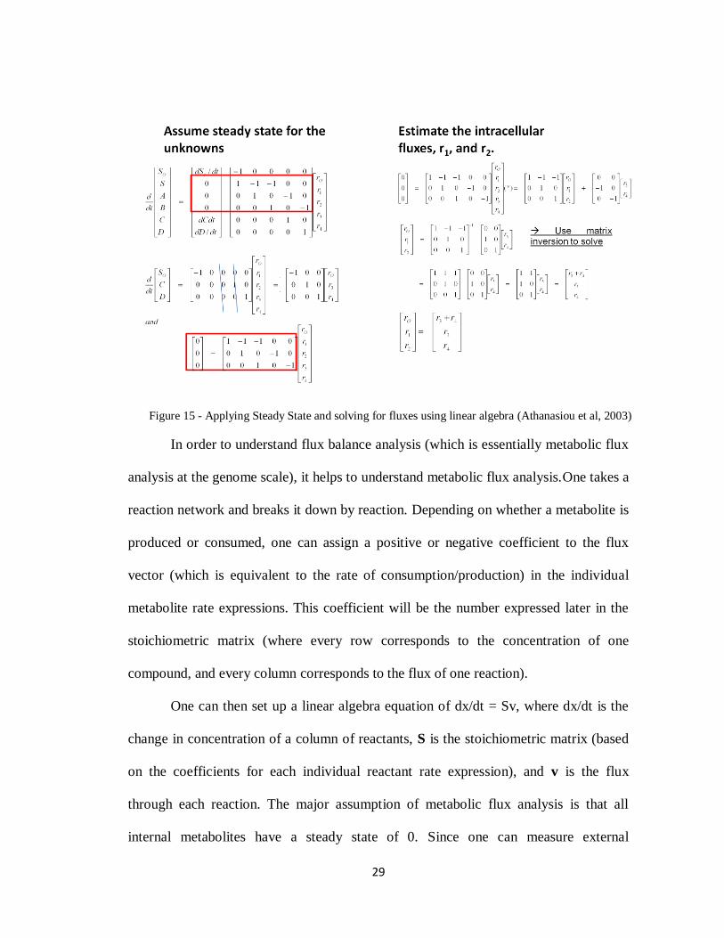
In order to understand flux balance analysis (which is essentially metabolic flux

analysis at the genome scale), it helps to understand metabolic flux analysis.One takes a

reaction network and breaks it down by reaction. Depending on whether a metabolite is

produced or consumed, one can assign a positive or negative coefficient to the flux

vector (which is equivalent to the rate of consumption/production) in the individual

metabolite rate expressions. This coefficient will be the number expressed later in the

stoichiometric matrix (where every row corresponds to the concentration of one

compound, and every column corresponds to the flux of one reaction).

One can then set up a linear algebra equation of dx/dt = Sv, where dx/dt is the

change in concentration of a column of reactants, S is the stoichiometric matrix (based

on the coefficients for each individual reactant rate expression), and v is the flux

through each reaction. The major assumption of metabolic flux analysis is that all

internal metabolites have a steady state of 0. Since one can measure external

Figure 15 - Applying Steady State and solving for fluxes using linear algebra (Athanasiou et al, 2003)

30

metabolites to obtain values, one can then set dx/dt=0 for the internal metabolites and

solve for the unknown fluxes using linear algebra (Figure 14 and Figure 15).

Flux balance analysis is metabolic flux analysis at the genome scale (Orth et al,

2010; Palsson, 2006). The major concepts from metabolic flux analysis are still the

same. S is still the stoichiometric matrix, and v is still the flux vector. Internal

metabolites still have an assumed steady state of 0. However, there are now a much

greater number of unknowns due to the larger system scale. With a larger system scale,

the number of unknowns exceeds number of knowns, resulting in a solution space, and

not a specific solution (Figure 16).

Figure 16 - Flux balance analysis – The allowable solution space is the set of all points satisfying all constraints. These constraints are represented by mass balance equations (which assure that any compound produced must equal the amount consumed at steady state) and capacity constraints (in the form of upper and lower bounds, which are usually based on experimental values). If a linear program has a non-empty bounded feasible region, then the optimal solution is always one of the corner points. (Orth et al, 2010).

In order to find an optimal solution within the solution space, one needs to apply

constraints, set an objective function ctv=Z, where c is a vector of weights indicating

how much each reaction contributes to the objective function, and maximize the

objective function. Ultimately, the objective function quantifies how much each

reaction contributes to overall phenotype. The mathematical representations of the

stoichiometric function and objective function set up a system of linear equations which

31

can be optimized using linear programming based algorithms to find the solution. Since

the constraints define a non empty and bounded solution space, the optimal solution

will always be at one of the corners (Figure 17 and Figure 18).

Figure 17 - (1) The feasible region of any linear program is always a convex set and (2) The iso-value line of a linear program objective function is always a linear function. Combining these two concepts, it follows that if a linear program has a non-empty, bounded feasible region, the optimal solution will always be one of the corner points (Arsham 2011).

32

Figure 18 - Flux Balance Analysis - Overall Approach (Orth et al, 2010)

2.3.2 - OPTKNOCK Algorithm

The OPTKNOCK algorithm is a bilevel programming algorithm (Figure 19),

meaning it takes the cellular objective function (as described in the previous flux

balance analysis section) and then runs it while also maximizing a surrounding

bioengineering objective (through the reaction knockouts) (Burgard et al, 2003).

33

Figure 19 - OPTKNOCK algorithm framework (Burgard et al, 2003)

Below is the Sv=0 function (the stoichiometric matrix multiplied by the flux

vector at steady state, as discussed in the section regarding FBA) rewritten within

context of maximizing flux towards the cellular objective (that is, the target pathway).

N

Mirrev

Msecr_only

Mrev

Next one accounts for gene deletion/reaction elimination; this constraint ensures

reaction flux is zero only if the yj is zero, i.e., reaction is knocked out .

34

M

The next step is combination of the reaction knockout and objective function

into the bilevel programming framework as illustrated in Figure 19. In other words, for

every reaction knockout the algorithm is also maximizing the cellular objective

function. Figure 20 shows the bilevel programming framework with the relevant

equations plugged in.

Figure 20 - Bilevel programming framework - maximizing cellular and bioengineering objectives (Burgard et al, 2003)

This is where we apply linear programming to find the solution (i.e., the

knockout which results in the highest flux redirected towards our target reactions).

There is a rule in linear programming where for every linear programming problem

(primal), there exists a unique optimization problem (dual) whose optimal objective

value is equal to that of the primal problem.

The dual problem associated with the OPTKNOCK inner problem is as follows.

35

Note that both the primal and dual problems are bounded by constraints in the form of

reaction knockouts, stoichiometric coefficients, and glucose uptake inputs. When

bounded by these constraints the primal and dual problems are equal to each other at

the optimal point. They can then be rewritten in order to solve for that optimum, which

corresponds to our solution (i.e., the knockout which results in the highest flux

redirected towards our target reactions).

36

2.4 - Formal Model Interface Design for Systems Integration

Now that the details for the semi-formal and formal modeling are in place, the

next issue to consider is interface design for the systems integration of models from

metabolic simulation and design space exploration.

The upper-half of Figure 19 is a Venn diagram of the relationship between SysML and

SBGN. Although the formalisms for both visualizations have been designed to serve

the needs of distinct communities, most of the distinctions are at the syntax level. There

is, in fact, a surprising overlap in features common to both representations. The notable

differences crop up in the visual representation of biology-specific glyphs and flow-

based modeling. The three SBGN diagrams (process diagrams, entity relationships

diagrams, and activity flow diagrams) are oriented respectively towards representing

temporal/mechanistic aspects of biochemical processes (e.g., metabolism), signaling

interactions between multistate entities (e.g., hormonal cascades), and biological

Figure 21 – Venn Diagram showing common and distinct features of SysML and SBGN, together with a framework for wrapping formal models with SysML interface constructs (e.g., ports).

37

influences (e.g., gene regulation). Process diagrams correspond in SysML notation to

structural constructs such as block diagrams, internal block diagrams, constrained block

diagrams and to some extent behavioral constructs such as state machine diagrams.

Entity relationship and activity flow diagrams correspond in the SysML notations to

behavioral constructs such as activity diagrams.

The defining characteristic of SBGN is its customization and use of visual

constructs for communication of ideas in biology. This is a good thing. Our supposition

is that SBGN can be combined with SysML, resulting in a system representation that

communicates ideas and acts as an interface to models for flow-based modeling (e.g.,

metabolic flux analysis and design explorations enabled through the use of

OPTKNOCK).

38

Chapter 3 – Metabolic Engineering Experiment

3.1 – Background

3.1.1 – Semi-formal Model Design - Goals

The second purpose of this paper is to demonstrate the effectiveness of the

framework discussed in Chapter 2, through application to a metabolic engineering

experiment.

This process begins with the semi-formal model design portion of our

framework (see the upper half of Figure 5) and the formulation of experimental

goals/scenarios, followed by the generation of requirements. Accordingly, the objective

of this experiment is to determine which reaction knockouts will maximize production

of the metabolite artemisinin in our genetically engineered strain of yeast. The

performance requirement is to maximize production of artemisinin. The functional

requirement is to maximize production subject to the constraint of maintaining

homeostasis.

The experimental procedure will determine the reaction knockouts using the

OPTKNOCK algorithm, and verify the predicted results using flux balance analysis

(FBA) simulations. Finally, we will present the results in visual form using a

combination of ad hoc metabolic engineering diagrams, SBGN, and SysML.

3.1.2- Motivation and History

Malaria is an infectious disease which affects nearly 200-250 million people and

kills nearly 700,000-1,000,000 people annually (World malaria report 2010). The

majority of those who die from infection live in poverty and cannot afford access to the

current anti-malarial drug standard, artemisinin. Consequently, any scientific advances

39

which can help lower the cost of artemisinin will translate into greater accessibility to

the drug worldwide. There have been two such major scientific advances in the past

five years. The first involves the reengineering of yeast to manufacture artemisinic acid,

a precursor to artemisinin (Ro et al, 2006), and the second, the creation of an alternative

“dihydro” pathway within yeast which enables synthesis of artemisinin in situ in the

presence of activated oxygen (Zhang et al, 2008).

3.1.3 – Advance 1: CYP71AV1/CPR Pathway

The high cost of Artemisinin stems from the extraction process of the drug from

the herb Artemisia annua (A. annua). Researchers at UC-Berkeley (hereafter referred to

as the Keasling group) have developed a procedure to cut the costs of drug

development by genetically engineering S. cerevisiae to produce artemisinic acid, a

precursor to artemisinin (Ro et al, 2006). By sourcing the drug from microbes instead

of plants, overall production time is decreased from months to days, and biomass

fraction increases from 1.9% to 4.5%, resulting in nearly two orders of magnitude of

productivity improvement.

The Keasling group’s strategy for producing artemisinin in S. cerevisiae

consists of three major steps:

1. Increase farnesyl pyrophosphate (FPP) production. As illustrated in Figure

22, this was done by upregulating the expression of tHMGR and ERG20,

and downregulating the expression of ERG 1-8, 11-13, 24-25.

40

Figure 22 - Schematic Representation of engineered artemisinic acid biosynthetic pathway in S. cerevisiae (Ro et al, 2006)

2. Introduce the amorphadiene synthase (ADS) gene into the genetic sequence

of S. cerevisiae in order to convert FPP to amorphadiene. To drive carbon

towards the inserted ADS pathway, the Keasling group uses a methionine-

repressible promoter to downregulate ERG9, the gene which expresses the

41

enzyme squalene synthase (red), and catalyzes the next step in the

mevalonate pathway in wild type yeast.

3. Insert genes CYP71AV1 and CPR from A. Annua to express enzymes from

the family cytochrome P450. These enzymes catalyze the oxidation of

amorphadiene to artemisinic acid.

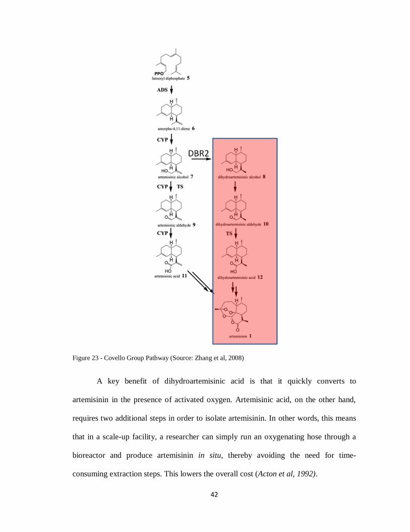
3.1.4 – Advance 2: DBR2 Pathway

A second group of researchers from the Canadian Plant Biotechnology Institute

(hereafter referred to as the Covello group), have determined that the gene DBR2, a

complementary DNA clone isolated from the flower buds of A. annua, corresponds to

artemisinic aldehyde double bond reductase activity in A. annua. As illustrated in the

highlighted portion of Figure 23, when S. cerevisiae uptakes the DBR2 gene, it creates

a new metabolic pathway from artemisinic alcohol to dihydroartemisinic acid (Zhang et

al, 2008).

In this pathway, artemisinic alcohol is converted to dihydroartemisinic alcohol

through the action of the double bond reductase enzyme, as regulated by the DBR2

gene. The double bond reductase eliminates the nonring double bond in artemisinic

alcohol by adding two atoms, resulting in the nickname “dihydro” pathway. While the

researchers were unable to identify what specific enzymes controlled for the continued

oxidization of dihydroartemisinic alcohol to dihydroartemisinic acid, oxidation did take

place, just as artemisinic alcohol oxidized to artemisinic acid in three steps.

42

Figure 23 - Covello Group Pathway (Source: Zhang et al, 2008)

A key benefit of dihydroartemisinic acid is that it quickly converts to

artemisinin in the presence of activated oxygen. Artemisinic acid, on the other hand,

requires two additional steps in order to isolate artemisinin. In other words, this means

that in a scale-up facility, a researcher can simply run an oxygenating hose through a

bioreactor and produce artemisinin in situ, thereby avoiding the need for time-

consuming extraction steps. This lowers the overall cost (Acton et al, 1992).

43

It is important to note that the new strains of yeast developed by the Covello

group contain both the “dihydro” pathway and Keasling Group pathways. While the

“dihydro” pathway presents productivity and economic advantages, the enzymes that

catalyze the formation of artemisinic acid from artemisinic alcohol play important roles

upstream within the overall yeast metabolic network. The creation of a new “dihydro”

only strain of yeast requires validation and verification to ensure that knockouts forcing

carbon to the “dihydro” route do not affect the performance of the overall metabolic

network.

3.2 - Formal Models for Metabolic Engineering

For the formal model sections of our multi-level framework, design space

exploration takes the form of determining which reaction knockouts will maximize

production of artemisinin. To do this, we run a mathematical abstraction of a yeast

model (as described earlier in Chapter 2) through the OPTKNOCK Algorithm. Then,

with the OPTKNOCK results in hand, the next step is to verify those results using flux

balance analysis (FBA) simulation. The latter coincides with the formal model analysis

portion of our framework.

3.2.1 - Tools

The simulation and design space exploration elements of the in silico

experiment employ MATLAB 7.11.0, a Tomlab/Cplex or Gurobi Linear Programming

solver, the COBRA Toolbox for MATLAB, and a suitable yeast model.

MATLAB 7.11.0 is a software package, which after more than two decades of

development, has become one of the standards for numerical analysis in the greater

scientific community. CPLEX is a linear programming solver designed by IBM. The

44

Tomlab plugin allows a MATLAB user to run CPLEX from within MATLAB. Gurobi

is an alternative linear programming solver free for academic users that runs within

MATLAB. The COBRA (Constraint Based Reconstruction and Analysis) Toolbox is a

package for MATLAB designed for in silico analysis of biological models. (Becker et

al,2007; Hyduke et al 2011). I will discuss yeast models further on in Section 3.2.4.

3.2.2 - Methodology

Figure 24 provides a high level view of the procedure for design space

exploration and simulation processes in the in silico experiment. The experimental

procedure consists of the following steps:

1. Prepare a SBML and COBRA compatible model of S. cerevisiae so that it

accurately reflects the genotypes of the strains in possession and load the

model into the COBRA Toolbox.

2. Set parameters and constraints of the simulated environment. This involves:

a. Define the media and nutrients available to the microbial culture;

b. Remove reactions from consideration that would be difficult or unreasonable

to knockout;

c. Establish the target reaction to maximize flux towards (for our purposes, the

artemisinin production biosynthetic pathway);

d. Declare biomass formation to be the constraint reaction;

3. With the aforementioned parameters and constraints in place, run the

OPTKNOCK algorithm. OPTKNOCK will output a list of suggested reactions

to knockout.

45

Figure 24 - Schematic of a Computational Metabolic Engineering Experiment

46

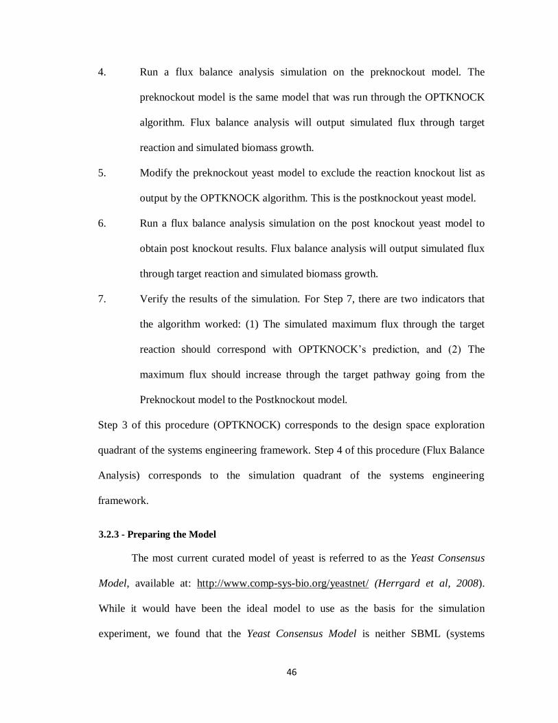
4. Run a flux balance analysis simulation on the preknockout model. The

preknockout model is the same model that was run through the OPTKNOCK

algorithm. Flux balance analysis will output simulated flux through target

reaction and simulated biomass growth.

5. Modify the preknockout yeast model to exclude the reaction knockout list as

output by the OPTKNOCK algorithm. This is the postknockout yeast model.

6. Run a flux balance analysis simulation on the post knockout yeast model to

obtain post knockout results. Flux balance analysis will output simulated flux

through target reaction and simulated biomass growth.

7. Verify the results of the simulation. For Step 7, there are two indicators that

the algorithm worked: (1) The simulated maximum flux through the target

reaction should correspond with OPTKNOCK’s prediction, and (2) The

maximum flux should increase through the target pathway going from the

Preknockout model to the Postknockout model.

Step 3 of this procedure (OPTKNOCK) corresponds to the design space exploration

quadrant of the systems engineering framework. Step 4 of this procedure (Flux Balance

Analysis) corresponds to the simulation quadrant of the systems engineering

framework.

3.2.3 - Preparing the Model

The most current curated model of yeast is referred to as the Yeast Consensus

Model, available at: http://www.comp-sys-bio.org/yeastnet/ (Herrgard et al, 2008).

While it would have been the ideal model to use as the basis for the simulation

experiment, we found that the Yeast Consensus Model is neither SBML (systems

http://www.comp-sys-bio.org/yeastnet/

47

biology markup language) nor COBRA compliant. Furthermore, although the protocol

behind SBML compliance can be extensive in its own right, a general overview of what

compatibility entails will suffice here (Hucka et al, 2003).

Within the model, there are two categories of classes: (1) reaction classes and

(2) metabolite classes. To be SBML compatible, each reaction class must have

attributes that include the abbreviation for the reaction, the name(s) of the compounds

in the reaction, the equation of the reaction, the cellular compartment in which the

reaction takes place (e.g., cytosol, mitochondria, ribosomes, etc), and the direction of

the reaction (i.e., irreversible, reversible). In order for the model to be COBRA

compatible, each reaction must also have a lower and upper bound with respect to flux

for each direction of the reaction, along with an objective function status (either 0 or 1).

For metabolite classes, SBML compatibility entails including attributes for a

compound’s abbreviation, name, and formula. COBRA compatibility requires the

attribute of compound charge. It is important to note that while additional attributes

could be included within classes, such as EC (enzyme class) numbers, KEGG (Kyoto

Encyclopedia of Genes and Genomes) abbreviations, and molecular weights, they are

not necessary for SBML/COBRA compatibility. Of all the attributes listed above, the

most important for the purposes of the simulation experiment is the equation, as the

mathematical abstraction of the S. cerevisiae model will be based on this attribute. A

practical caveat - because the equation is dependent on the compound abbreviations and

direction of reaction, it is important to verify that both of these attributes also

correspond correctly with the equations.

Since the consensus yeast model was neither SBML nor COBRA compatible,

48

the next best choice was the iMM904 model (note that i stands for in silico, MM are

the initials of Monica Mo, who developed the model, and 904 is the number of genes in

the model) (Mo et al, 2009). The iMM904 model corresponds to the genetic makeup of

the wild type yeast strain S288C.

The yeast strains used in the Sriram lab are derivatives of yeast strain W303

from the Covello group, which has some differences from S288C with respect to

genetic makeup that have to be accounted for in the model:

S288C has the genotype: MATα SUC2 gal2 mal mel flo1 flo8-1 hap1 ho bio1 bio6

(Mortimer et al, 1986)

W303 has the genotype: MATa/MATα {leu2-3,112 trp1-1 can1-100 ura3-1 ade2-1 his3-

11,15} (Thomas et al, 1989)

When observing genotypes, it is important to note that capitalized letters are

working versions of the gene, and lower case letters are nonfunctional. Nonfunctional

genes can be restored to functional status when the cell uptakes a plasmid with the

gene.

The following plasmids were taken up by the W303 genotype to generate the

Sriram lab’s strains: (Zhang et al, 2008)

Strain 1: pESC-HIS, pESC-LEU, pYES-DEST52-GUS2

Strain 2: pESC-HIS-FPS-ADS, pESC-LEU-CYP-CPR, pYES-DEST52-GUS.

Strain 3: pESC-HIS-FPS-ADS, pESC-LEU-CYP-CPR, pYES-DEST52-DBR2

49

Each plasmid contained its own strain-dependent combination of pathways.

Being a control, Strain 1 received a control plasmid which reactivated histidine,

reactivated leucine, and contained a placeholder gene DEST52-GUS. Strain 2 contained

the artemisinic acid production pathway which consists of the ADS genes and the CYP-

CPR genes (refer Figure 22) along with the DEST52-GUS gene. Strain 3 contained the

genes coding for the artemisinic acid pathway and the dihydroartemisinic pathway

(attached with the DEST-52 gene).

For the purposes of modifying the model, this means that between S288C and

W303, only the SUC2 gene and corresponding reaction need to be removed, as the rest

of the genes are nonfunctional. An additional point to note is that the active versions of

his, leu and ura3-52 in the model represent the yeast strain taking up the plasmids

containing HIS, LEU, and DEST52. By taking up the plasmids, the yeast cell restores

the ability to synthesize histidine, leucine, and uracil. After accounting for all of the

aforementioned factors in the W303 strain, this leaves the genes trp1, ade2, and can1-

100. Any reactions controlled by active versions of these genes would have to be

removed from the model in order to reflect the experimental strain. Table 3 contains a

summary of all reactions removed from the iMM904 model. It coincides with Strain 1.

Table 3 - Preparing the Yeast model – Strain 1

REMOVALS

(STRAIN 1)

Gene RXN RXN Description

SUC2 DGGH alpha-D-glucoside glucohydrase

trp1 PRAIi phosphoribosylanthranilate isomerase (irreversible)

ade2 AIRCr phosphoribosylaminoimidazole carboxylase

can1-

100 ARGt2r L-arganine reversible transport via proton symport

50

When adding reactions to the model, it helps to reexamine the plasmids taken

up by the strains. Every one of the capitalized genes, except for the promoters (pESC

and pYES) will have to be accounted for in the strain reactions.

As a case in point, Strain 1 took up the pESC-HIS, pESC-LEU, pYES-DEST52-

GUS2 plasmids. HIS, LEU, and DEST52 are already present in the model and GUS2

regulates the expression of the enzyme beta-glucuronidase. However, none of the

reactants for the reactions that beta-glucuronidase controls were present in the model as

metabolites, meaning that this enzyme would be essentially inactive, and therefore not

required in the model. This is why DEST52-GUS 52 is referred to as a placeholder

earlier (as it is simply there as a control until it functions as a delivery vehicle for

DBR2 in strain 3).

Strain 2 took up the plasmids pESC-HIS-FPS-ADS, pESC-LEU-CYP-CPR,

pYES-DEST52-GUS2. HIS, LEU, and DEST52 are already present in the model.

Referring back to Figure 22 , one will remember that the FPS-ADS gene controls the

conversion of FPP to amorphadiene, and that CYP/CPR controls the 3 step oxidation of

artemisinic alcohol to artemisinic acid. While Strain 2 represents the Keasling group’s

pathway in the simulation experiment, it is important to remember that the W303 strain

is still genetically different overall from the Keasling group’s strain, BY4742. Thus, a

true direct comparison between the Keasling group’s results and this experiment may

not be possible. In order to represent the genotype of strain 2, the reactions in Table 4

were added to the model for strain 1 (Table 3).

51

Table 4 - Preparing the Yeast model - Strain 2

ADDITIONS

(STRAIN 2) (in addition to strain 1 removals)


FPS-ADS ADS Amorpha-4,11-diene synthase

CYP-CPR ARTALC_CYP7 amorph-4,11-diene to artemisinic alcohol

CYP-CPR ARTALD_CYP7 artemisinic alcohol to artemisinic aldehyde

CYP-CPR ARTACID artemisinic aldehyde to artemisinic acid

Strain 3 took up the plasmids pESC-HIS-FPS-ADS, pESC-LEU-CYP-CPR, and

pYES-DEST52-DBR2 plasmids. Referring to Figure 23, one will remember that the

DBR2 gene controls for the conversion of artemisinic alcohol to dihydroartemisinic

alcohol, i.e., the “dihydro” pathway. Strain 3 essentially represents the Covello group’s

strain in the simulation experiment, which included both the Keasling group’s pathway

and the “dihydro” pathway. The reactions listed in Table 5 were added to the strain 2

model (seeTable 3 and Table 4 ) to accurately represent the strain 3 genotype.

Table 5 - Preparing the Yeast Model - Strain 3

ADDITIONS

(STRAIN 3)


DBR2 DBR2 artemisinic aldehyde to dihydroartemisinic aldehyde

DBR2 DARTACID dihydroartemisinic aldehyde to dihydroartemisinate

3.2.4 - Setting Parameters and Constraints

Preparation of the simulation environment begins with the setting of parameters

and constraints for the availability of amino acids and nutrients from the media (Becker

et al, 2007; Hyduke et al, 2011). Since the laboratory media is galactose based, the

simulation set galactose uptake to 11.1 mol•gDW-1

• h-1. And since the W303 derived

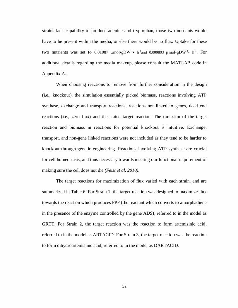
52

strains lack capability to produce adenine and tryptophan, those two nutrients would

have to be present within the media, or else there would be no flux. Uptake for these

two nutrients was set to 0.01087 mol•gDW-1• h

-1and 0.009803 mol•gDW

-1• h

-1. For

additional details regarding the media makeup, please consult the MATLAB code in

Appendix A.

When choosing reactions to remove from further consideration in the design

(i.e., knockout), the simulation essentially picked biomass, reactions involving ATP

synthase, exchange and transport reactions, reactions not linked to genes, dead end

reactions (i.e., zero flux) and the stated target reaction. The omission of the target

reaction and biomass in reactions for potential knockout is intuitive. Exchange,

transport, and non-gene linked reactions were not included as they tend to be harder to

knockout through genetic engineering. Reactions involving ATP synthase are crucial

for cell homeostasis, and thus necessary towards meeting our functional requirement of

making sure the cell does not die (Feist et al, 2010).

The target reactions for maximization of flux varied with each strain, and are

summarized in Table 6. For Strain 1, the target reaction was designed to maximize flux

towards the reaction which produces FPP (the reactant which converts to amorphadiene

in the presence of the enzyme controlled by the gene ADS), referred to in the model as

GRTT. For Strain 2, the target reaction was the reaction to form artemisinic acid,

referred to in the model as ARTACID. For Strain 3, the target reaction was the reaction

to form dihydroartemisinic acid, referred to in the model as DARTACID.

53

Table 6 - List of Target Reactions

Strain RXN RXN Description RXN Equation

RXN

Compartment

1 GRTT

Geranyl-

transtransferase

grdp[c] + ipdp[c] ->

frdp[c] + ppi[c]

Sterol

Metabolism

2 ARTACID artemisinic aldehyde to artemisinic acid

artCHO[c] + nadph[c] <=>

artCOOH[c]

Artemisinin

Pathway

3 DARTACID

dihydroartemisinic

aldehyde to

dihydroartemisinate

dhartCHO[c] + nadp[c] +

h2o[c] <=> dhartCOO[c]

+ nadph[c] + 2 h[c]

Dihydro

Artemisinin Pathway

3.2.5 - OPTKNOCK Results and FBA Verification

Table 7 is a summary of the results of the metabolic engineering experiment.

Table 7 - OPTKNOCK Results and Verification (Units: mol•gDW-1• h-1)

STRAIN 1

Growth Rate of

Yeast Cells Targeted RXN = GRTT

Trial

# Suggested KO

Optknock

Prediction

PreKO

Biomass

PostKO

Biomass

PreKO Max

Flux

PostKO

Max Flux

1 HICITDm 2.5098 0.1098 0.057 2.4393 2.5209

2 HACNHm / UGLT 2.5098 0.1098 0.057 2.4393 2.5209

3 ADK1 / SACCD1 / G6PDH2 2.5098 0.1098 0.057 2.4393 2.5209

STRAIN 2

Growth Rate of

Yeast Cells

Targeted RXN =

ARTACID

Trial # Suggested KO

Optknock Prediction

PreKO Biomass

PostKO Biomass

PreKO Max Flux

PostKO Max Flux

1 HACNHm 2.593 0.1098 0.057 2.5199 2.6045

2

ACONT /

HICITDm 2.593 0.1098 0.057 2.5199 2.6045

3 SACCD2 2.593 0.1098 0.057 2.5199 2.6045

STRAIN 3

Growth Rate of

Yeast Cells

Targeted RXN =

DARTACID

Trial # Suggested KO

Optknock Prediction

PreKO Biomass

PostKO Biomass

PreKO Max Flux

PostKO Max Flux

1 SACCD2 2.558 0.1098 0.057 2.4859 2.5694

2 ADK1 / SACCD2 2.558 0.1098 0.057 2.4859 2.5694

3 HICITDm / ILETA 2.558 0.1098 0.057 2.4859 2.5692

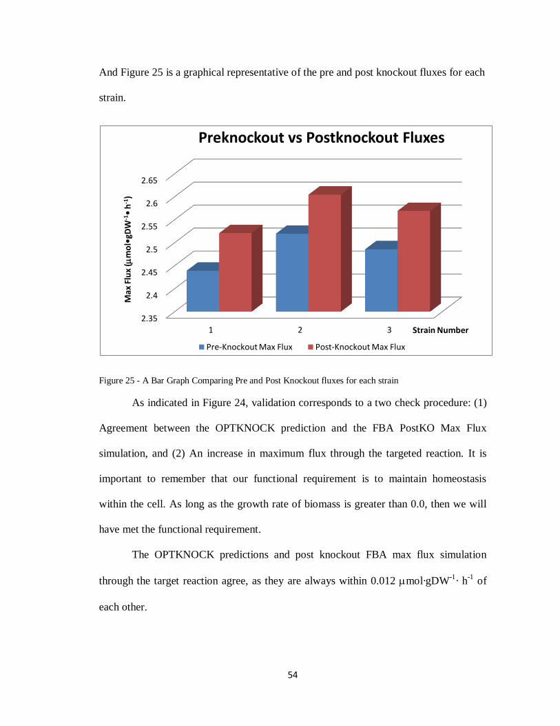
54

And Figure 25 is a graphical representative of the pre and post knockout fluxes for each

strain.

Figure 25 - A Bar Graph Comparing Pre and Post Knockout fluxes for each strain

As indicated in Figure 24, validation corresponds to a two check procedure: (1)

Agreement between the OPTKNOCK prediction and the FBA PostKO Max Flux

simulation, and (2) An increase in maximum flux through the targeted reaction. It is

important to remember that our functional requirement is to maintain homeostasis

within the cell. As long as the growth rate of biomass is greater than 0.0, then we will

have met the functional requirement.

The OPTKNOCK predictions and post knockout FBA max flux simulation

through the target reaction agree, as they are always within 0.012 mol·gDW-1

· h-1

of

each other.

2.35

2.4

2.45

2.5

2.55

2.6

2.65

1 2 3

Max

Flu

x (

mo

l•gD

W-1

• h

-1)

Strain Number

Preknockout vs Postknockout Fluxes

Pre-Knockout Max Flux Post-Knockout Max Flux

55

A comparison of the preKO and postKO max fluxes through the target pathway

always showed an increase of 0.080-0.085 mol·gDW-1

· h-1. When comparing pre and

post knockout flux, it did not seem like this increase was particularly significant (with

the change in flux between pre and post knockout models being less than 0.1). We

would not anticipate results this small would show up experimentally.

There is, however, a trend within these results, which will become more

apparent with visualization. SACCD1, SACCD2, HACNHm, and HICITDm are all

suggested knockouts that lie in the same pathway of lysine formation, the latter

stemming from the combination of alpha keto glutarate and acetyl CoA (refer Figure

26). One can logically hypothesize that knocking out reactions in this pathway would

cause a buildup of acetyl CoA. This strategy is supported by Figure 22 and Figure 23,

where one can see that acetyl CoA is the primary metabolite feeding into the

mevalonate pathway, the site of our inserted genetically engineered pathways. Thus, an

increase in acetyl CoA could feasibly translate into an increase in flux through our

target pathways. From this perspective, the suggested knockouts make sense. Rather

than having to produce its own lysine, the cell could obtain the amino acid lysine from

the medium. In fact, it is possible that experimenting with the makeup of the media may

result in higher and more significant changes in flux when comparing the pre and post

knock out models.

56

Figure 26 - Lysine Metabolic Pathway

57

3.3 – Semi-Formal Models for Metabolic Engineering

The purpose of this section is to compare and contrast the strengths and

weaknesses of the three types of abstraction (ad-hoc, SBGN, and SysML) for

visualization of experimental results.

Two key concepts associated with visualization are information hiding and

encapsulation. With respect to the experiment, information hiding refers to the omission

of all irrelevant pathways of interest, and encapsulation refers to the grouping of sets of

reactions by their pathways. From the perspective of designing an efficient metabolic

process, the most relevant pathways are: (1) The mevalonate pathway (on which our

target reactions were inserted), (2) Glycolysis / the TCA cycle (on which a key

metabolite, acetyl CoA, is produced), and (3) The pathway of lysine formation, which

stems from the combination of alpha keto glutarate and acetyl CoA. These pathways are

highlighted in Figure 27. Visualization techniques that draw attention towards these

pathways, and eliminate information not needed for decision-making, will be helpful.

The first type of visualization, (see for example, Figure 27) employs an ad hoc

notation for the visual display of yeast metabolism: use of this notation is state-of-the-art

practice in the metabolic engineering field. This notation is ad hoc because it comes from

a commercial toolbox and is not an industry standard. The ad hoc notation places an

emphasis on showing flux and giving a bird’s eye view of the metabolic system. The

second type of visualization (see Figure 28) involves an SBGN compliant diagram based

on a single knockout run of strain 2. Its emphasis is on showing the topological

connections between the metabolites. The third type of visualization (see Figure 29 and

Figure 30) is a set of two SysML compliant diagrams that show a single knockout run of

58

strain 2. Figure 29 is an internal block diagram that emphasizes the connectivity of the

reactions through which the carbon atoms flow. Figure 30 is a parametric diagram that

shows how flow can be modeled using constraints.

3.3.1 - Ad Hoc Abstraction

This section briefly discusses the key visual abstractions, and advantages and

disadvantages of the ad hoc visualization (associated with the COBRA Toolbox).

Key Abstractions. The labeled segments act as abstractions, hiding information specific

to nodes and encapsulating nodes on the same pathway together. Experienced Metabolic

Engineers will have an intuitive understanding of the labeled pathways. Hence, they may

not need to see individual nodes within a labeled segment in order to understand what is

going on within the networks. Engineers without a metabolic engineering background

may have difficulty understanding how the suggested knockout drives metabolic traffic

towards Acetyl CoA and the artemisinic acid pathway.

Advantages. The primary purpose of this ad hoc diagram notation is to provide a bird’s

eye view of yeast metabolism. In Figure 27, each black node represents a compound,

with each line between nodes representing a reaction. There are well over a thousand

reactions represented here, so this type of diagram does a great job of showing how

complex yeast metabolism is (with the pathways highlighted in yellow being our

pathways of interest). The metabolic flux is represented via color and line thickness (in

this case pink and blue show corresponding areas of high metabolic traffic). This type of

representation can be useful in virtual space, since it allows for zooming in, zooming out,

and creating external links to websites with information on each reaction / compound.

59

Figure 27 –A Non standard de facto Visual Abstraction generated using BIGG and the COBRA Toolbox (Hyduke et al, 2011))

60

Disadvantages. First, it is impossible to see what is going on at a more detailed level

without zooming in. A second disadvantage is the lack of clarity in how the different

pathways represented as segments connect to each other. This problem can be mitigated

by representing flux with color and line thickness is an intuitive way to show metabolic

traffic; however, this potential solution is not device independent. To summarize,

generally speaking, the COBRA Toolbox is relatively limited in terms of its visualization

capabilities. The text-based layout means that the visual layout is rigid, with only the

colors and line thickness of metabolic traffic being capable of modification (Hyduke et al,

2011; Schellenberger et al, 2010).

Figure 28 – SBGN compliant notation, generated using VANTED and SBGN-ED software (Junker et al, 2006;

Czauderna et al, 2010). The target pathway for flux is highlighted and the suggested knockouts are

crossed out.

61

3.3.2 - SBGN Abstraction

This section briefly discusses the key abstractions, and advantages and

disadvantages of SBGN as a visual formalism.

Key Abstractions. The abstractions specific to SBGN and biology are as follows: simple

molecules are represented by circles, with more complex compounds represented by

rectangles with rounded corners. Repeated compounds are partially filled in. Reactions

are represented by squares. Enzymes are marked by compounds linked to circles which

modify the squares (See Figure 10 in Section 2.2.2 for the complete list of glyphs). The

next important abstraction in SBGN is the subgraph. As illustrated in Figure 28, the

subgraph is the functional equivalent of a black box in systems engineering and enables

the user to condense a series of relevant reactions into a subgraph with links connecting

the subgraph to other metabolites. Subgraphs are crucial abstractions as they enable

encapsulation of a group of reactions in a pathway while hiding the details of each

individual reaction, thereby freeing up space in the layout for the reactions of interest.

Advantages. SBGN diagrams provide a visual representation for how the suggested

knockout reaction (conversion of but-1-ene-1,2,4-tricarboxylate to homoisocitrate as

catalyzed by the enzyme homoacontinate hydratase) drives traffic back towards Acetyl

CoA, the key bottleneck. A second benefit stems from their use of biology-specific

glyphs – that is, glyphs that allow for a quick understanding of the types of compounds

present in a pathway.

Disadvantages. The main disadvantage of SBGN, at least with respect to the needs of the

metabolic experiment, is lack of a formal methodology for modeling flow. Metabolic flux

is the key parameter for determining activity in metabolic networks. As a quick

62

workaround and for the time being, we were able to annotate some flow values, but there

will need to be a formal abstraction for flux in order to actually model parameters and

constraints.

Figure 29 - SysML Visual Model for Pathways of Interest The target pathway for flux is highlighted and the suggested knockouts are crossed out.

63

Figure 30 - Parametric Diagram defining parameters and constraints between MICITD and HACNH reactions

3.3.3 - SysML Abstraction

In this section, we briefly describe the key visual abstractions, and advantages and

disadvantages of SysML as a visual formalism for supporting metabolic experiments.

Key Abstractions. SysML provides a wide range of diagram types for describing system

structure, system behavior, requirements, and parametric relationships within a system.

SysML is deliberately designed to be application neutral. For metabolic engineering, the

64

most useful types of diagram are black boxes and block diagrams. See, for example,

Figure 29 and Figure 30. The key abstractions for the SysML visualization are the black

boxes and the block diagram. Black boxes have a one to one relationship with the

subgraphs of SBGN, thereby encapsulating a series of reactions together, and hiding the

details of each individual reaction. The block diagram represents a reaction, with the

reactants, products, catalyst listed as attributes, with :mf at each port representing

metabolic flux. It should be noted that the decision to use reactants, products, and

enzymes as attributes was not mandated by the SysML specification, but a decision on

our end to show how SysML could add an additional layer of abstraction over the SBGN

models, resulting in a fewer number of total entities.

In order to show how SysML can model constraints and flows, we have also

included a parametric diagram. For example, Figure 30 provides a detailed view of the

constraints governing the MCITD and HACNH reactions. Using parametric diagrams we

can set constraints based on the reaction stoichiometry (in this case 1:1), and

experimental design (knockout indicates flux = 0). We were able to combine both

constraints into one constraint using an if then statement and a block representing the

external user. Since our purpose in creating the visualization prototype was only to make

a point, we focused only on these two reactions. A more comprehensive example would

attach constraints and parameters to every reaction in the network. The key point to note

is that one can proceed through an entire pathway applying the rules and commands as

set by the constraints, while outputting the associated parameters for tracking purposes.

This capability would be an essential part of SysML becoming a central interface in a

metabolic engineering design framework.

65

Advantages. As an established standard visual notation, SysML offers a lot of flexibility

for the representation of metabolic networks. It has a formal methodology for

representing flow, and it can show the topological connectivity of separate pathways.

Looking ahead, BIOMEMS devices and systems are almost certain to become

commonplace. Having a notation specific to machines also applied to biology may be

useful for creating visual abstractions of machines interacting with living objects.

Disadvantages. The main disadvantage of SysML is its lack of support for biology-

specific glyphs. To most straightforward compensation for this shortcoming is to write

additional text (e.g., this is an enzyme) on the diagram. However, for all but the simplest

systems, diagrams would quickly become cluttered, thereby obscuring a designer’s ability

to understand the network structure and behavior. We suggest that this limitation can be

overcome by integrating SysML with SBGN or whatever graphical user interface (GUI)

the researcher prefers.

3.4 - Systems Integration for Metabolic Engineering

In Section 2.4, we discussed the possibility of using SysML as a centerpiece

integrator, designed to link the four quadrants of the multilevel framework shown in

Figure 5 and Figure 6. This section will discuss how the metabolic engineering

experiment fits into the systems engineering framework (see Figure 31) and offer

perspective on how a metabolic engineering experiment could fit into the framework

through the use of SysML wrappers.

Goals / Scenarios (Semi-Formal models)

The pathway from goals and scenarios to requirements can be documented with Use Case

and Requirements Diagrams. Requirements leads to the generation of experimental

66

objectives and constraints. For example, our metabolic experiment has the standard

functional requirement to maintain a living state in the yeast cell, and the performance

requirement of maximizing artemisinin production in the yeast metabolism. We

hypothesize that once the standard functional requirements have been correctly expressed

in SysML, theoretically, a researcher could automate the validation and verification of the

requirement for every result generated in the formal models. By automating the back-

and-forth flow of data between the semi-formal and formal models, the time needed in

order to determine the experimental feasibility of computational predictions will be

reduced.

Visual Abstraction (Semi-Formal models)

As highlighted in Figure 21, there is a 1:1 relationship between many of the SBGN

process diagram components and the components of a SysML internal block diagram.

Recent research has shown that with XML representations for SysML and SBGN in

place, it is certainly feasible to simultaneously display both types of diagrams, and

synchronize user interface actions across the visualizations (Delgoshaei and Austin,

2011). While there are no standards for displaying color/size based flows, constraints and

parameters can certainly propagate through the SysML wrapper in the internal code and

give output values for metabolic flux. Metabolic flux values can also be included as

annotations in SBGN, or whatever visual format is preferred by the end user. With

respect to the in silico experiment, no single diagram type provides superior visual

support for understanding how choking the lysine pathway redirected flux to the

artemisinin producing pathways. Therefore, for the time being, this means that multiple

forms of visualization are essential.

67

Figure 31 - Systems Integration - Plugging the in silico metabolic engineering experiment into the Systems Engineering framework

68

Design Space Exploration and Simulation (Formal models)

In the metabolic experiment both the design space exploration (OPTKNOCK) and

simulation (FBA) were run using MATLAB and the COBRA Toolbox. Looking forward,

we are not locked into this computational framework. There are, in fact, already

interfaces on the market designed to wrap MATLAB code and scripts in a SysML

interface (Bajaj et all, 2011). We note that because SysML provides support for flow-

based modeling, flows of data to and from the wrapper will be possible. Together, these

features can work together to give researchers options. A technically experienced

researcher may prefer to run the experiment at the MATLAB layer. Less technically

experienced researchers will be provided with a way to access the same experiment by

interacting with the graphical SBGN layer.

69

Chapter 4 – Conclusion

4.1 - Summary

This paper has served two purposes: (1) We have proposed a multi-level

framework for the synthesis, analysis and design of metabolic systems, and (2) We have

applied this framework to a metabolic engineering experiment.

Design activities in the proposed framework are divided into four quadrants, and

are based on formal models and semi-formal models for a network of linked system

design and system analysis components. Goals and scenario analysis links semi-formal

modeling to formal approaches to system design. Visual abstractions (e.g., SysML) are

linked to formal approaches to system analysis. Design space exploration employs formal

approaches to system design. Computer simulation employs formal approaches to system

analysis.

Various aspects of this framework have been exercised by working step by step

through an in silico metabolic engineering experiment. The results indicate that

interruption of the pathway driving carbon from alpha-keto glutarate and acetyl CoA

towards lysine would maximize flux through our target pathways, increasing artemisinin

production. This makes sense because interruption of the lysine production pathway

causes a buildup of acetyl CoA, which feeds into the mevalonate pathway, the insertion

site of the genetically engineered pathways for artemisinin production. Our framework

corresponds to the following aspects of the in silico experiment:

(1) Goals/scenarios involved maintaining a living state and maximizing

production of the metabolite artemisinin;

70

(2) Visual abstraction involved ad hoc, SBGN, and SysML diagrams, which

placed special emphasis on showing how reaction knockouts in the lysine pathway could

redirect flux towards the artemisinin producing pathway;

(3) Design space exploration took the form of running a yeast model through the

OPTKNOCK algorithm; and

(4) Computer simulation took the form of flux balance analysis.

4.2 - Future Work

Biological systems are now considered to be the Holy Grail of systems

complexity. This study has been a first step. Although the scope of this study has been

restricted to single-celled organisms in the form of yeast, these systems are still complex

systems, with massive numbers of components which interact in a combinatorial fashion.

As we work with higher-level organisms, increase our technological capabilities, and

learn more about biology, both observational complexity and system design complexity

will increase. It is evident that without new approaches to design space exploration and

metabolic systems simulation, this will result in a large gap between design and

validation capabilities and what is required from a productivity standpoint.

The software and systems engineering community has handled increasingly

complex systems by developing the ability to solve problems at higher levels of

abstraction. This strategy offers a pathway forward for the biological world to emulate.

As of 2011, SysML is the benchmark visual modeling language for the field of systems

engineering, and has been used as both a visual abstraction and interface for various

portions of complex systems engineering projects.

71

Looking ahead, our proposed multilevel framework needs to take advantage of

SysML, as a visual abstraction, as a construct for module wrapping, and as a mechanism

for creating heterogeneous design environments composed from mixtures of formal and

semi-formal models.

72

References

1. Acton, N., & Roth, R. J. (1992). On the conversion of dihydroartemisinic acid into

artemisinin. The Journal of Organic Chemistry, 57(13), 3610-3614.

2. Agrawala, M., Li, W., & Berthouzoz, F. (2011). Design principles for visual

communication. Communications of the ACM, 54(4), 60.

3. Aregawi, M., & World Health Organization. (2010). World malaria report 2010.

Geneva: World Health Organization.

4. Arsham, Hossein. (2011). Deterministic Modeling: Linear Optimization with

Applications. Retrieved November 16, 2011, from

http://home.ubalt.edu/ntsbarsh/opre640a/partVIII.htm#rplp

5. Athanasiou, Kyriacos & Ka-Yiu San. (2003). Metabolic Flux Analaysis. Retrieved

February 22,2011, from http://www.ruf.rice.edu/~bioewhit/courses/bioe321

6. Austin, M. (2011). Information-Centric Systems Engineering, Class Notes for

ENSE 621 System Concepts, Processes and Issues, Institute for Systems

Research, University of Maryland, College Park, MD 20742, September 2011.

7. Bajaj, M., Zwemer,, D., Peak, R., Phung, A., Scott, A., & Wilson, M. (2011).

Satellites to Supply chains, Energy to Finance - SLIM for Model-Based Systems

Engineering. INCOSE International Symposium.

8. Becker, S. A., Feist, A. M., Mo, M. L., Hannum, G., Palsson, B. Ø., & Herrgard,

M. J. (2007). Quantitative prediction of cellular metabolism with constraint-based

models: the COBRA Toolbox. Nature Protocols, 2(3), 727-738.

9. Bernhard O. Palsson. (2006). Systems Biology: Properties of Reconstructed

Networks (1st ed.). New York: Cambridge University Press.

73

10. Boyle, N. R., & Morgan, J. A. (2011). Computation of metabolic fluxes and

efficiencies for biological carbon dioxide fixation. Metabolic Engineering, 13(2),

150-158.

11. Burgard, A. P., Pharkya, P., & Maranas, C. D. (2003). OPTKNOCK: a bilevel

programming framework for identifying gene knockout strategies for microbial

strain optimization. Biotechnology and Bioengineering, 84(6), 647-657.

12. Covello, P. S., Teoh, K. H., Polichuk, D. R., Reed, D. W., & Nowak, G. (2007).

Functional genomics and the biosynthesis of artemisinin. Phytochemistry, 68(14),

1864-1871.

13. Czauderna, T., Klukas, C., & Schreiber, F. (2010). Editing, validating and

translating of SBGN maps. Bioinformatics, 26, 2340-2341.

14. Delgoshaei P. and Austin M.A., Software Design Patterns for Ontology-Enabled

Traceability. Ninth Annual Conference on Systems Engineering Research (CSER

2011), Redondo Beach, CA, April 14-16, 2011.

15. Endy, D. (2005). Foundations for engineering biology. Nature, 438(7067), 449-

453.

16. Feist, A. M., Zielinski, D. C., Orth, J. D., Schellenberger, J., Herrgard, M. J., &

Palsson, B. Ø. (2010). Model-driven evaluation of the production potential for

growth-coupled products of Escherichia coli. Metabolic Engineering, 12, 173-186.

17. Friedenthal, S. (2009). A practical guide to SysML : the systems modeling

language ([Neuaufl.].). Amsterdam [u.a.]: Elsevier Morgan Kaufmann OMG.

74

18. Gregory N. Stephanopoulos, Nielsen, Jens, & Aristidou, Aristos. (1998).

Metabolic Engineering: Principles and Methodologies (1st ed.). San Diego:

Academic Press.

19. Herrgård, M. J., Swainston, N., Dobson, P., Dunn, W. B., Arga, K. Y., Arvas, M.,

Büthgen, N., et al. (2008). A consensus yeast metabolic network reconstruction

obtained from a community approach to systems biology. Nature Biotechnology,

26(10), 1155-1160.

20. Hucka, M., Finney, A., Sauro, H. M., Bolouri, H., Doyle, J. C., Kitano, H., and the

rest of the SBML Forum:, et al. (2003). The systems biology markup language

(SBML): a medium for representation and exchange of biochemical network

models. Bioinformatics, 19(4), 524-531.

21. Hyduke, D., Hyduke, D., Schellenberger, J., Que, R., Fleming, R., Thiele, I., Orth,

J., et al. (2011). COBRA Toolbox 2.0. Protocol Exchange.

22. Junker, B. H., Klukas, C., & Schreiber, F. (2006). VANTED: a system for

advanced data analysis and visualization in the context of biological networks.

BMC Bioinformatics, 7, 109.

23. Kim, J., & Reed, J. L. (2010). OptORF: Optimal metabolic and regulatory

perturbations for metabolic engineering of microbial strains. BMC Systems

Biology, 4, 53.

24. Lun, D. S., Rockwell, G., Guido, N. J., Baym, M., Kelner, J. A., Berger, B.,

Galagan, J. E., et al. (2009). Large-scale identification of genetic design strategies

using local search. Molecular Systems Biology, 5.

75

25. Mo, M. L., Palsson, B. Ø., & Herrgård, M. J. (2009). Connecting extracellular

metabolomic measurements to intracellular flux states in yeast. BMC Systems

Biology, 3(1), 37.

26. Moodie, S., Moodie, S., Le Novere, N., Demir, E., Mi, H., & Villeger, A. (2011).

Systems Biology Graphical Notation: Process Description language Level 1.

Nature Precedings.

27. Mortimer, R. K., & Johnston, J. R. (1986). Genealogy of principal strains of the

yeast genetic stock center. Genetics, 113(1), 35-43.

28. Le Novère N, Hucka M, Mi H, Moodie S, Schreiber F, Sorokin A, Demir E,

Wegner K, Aladjem MI, Wimalaratne SM, Bergman FT, Gauges R, Ghazal P,

Kawaji H, Li L, Matsuoka Y, Villéger A, Boyd SE, Calzone L, Courtot M,

Dogrusoz U, Freeman TC, Funahashi A, Ghosh S, Jouraku A, Kim S, Kolpakov F,

Luna A, Sahle S, Schmidt E, Watterson S, Wu G, Goryanin I, Kell DB, Sander C,

Sauro H, Snoep JL, Kohn K, Kitano H. The Systems Biology Graphical Notation.

Nat Biotechnol. 2009.

29. OMG: Systems Modeling Language v 1.2 (2010)

http://www.omgsysml.org/#Specification

30. Orth, J. D., Thiele, I., & Palsson, B. Ø. (2010). What is flux balance analysis?

Nature Biotechnology, 28(3), 245-248.

31. Ro, D.-K., Paradise, E. M., Ouellet, M., Fisher, K. J., Newman, K. L., Ndungu, J.

M., Ho, K. A., et al. (2006). Production of the antimalarial drug precursor

artemisinic acid in engineered yeast. Nature, 440(7086), 940-943.

http://www.omgsysml.org/#Specification

76

32. Sangiovanni-Vincentelli A., McGeer P.C., Saldanha A., Verification of Electronic

Systems : A Tutorial, Proceedings of the 33rd Design Automation Conference,

Las Vegas, 1996.

33. Schellenberger, J., Park, J. O., Conrad, T. M., & Palsson, B. Ø. (2010). BiGG: a

Biochemical Genetic and Genomic knowledgebase of large scale metabolic

reconstructions. BMC Bioinformatics, 11(1), 213.

34. Thomas, B. J., & Rothstein, R. (1989). The genetic control of direct-repeat

recombination in Saccharomyces: the effect of rad52 and rad1 on mitotic

recombination at GAL10, a transcriptionally regulated gene. Genetics, 123(4),

725-738.

35. Tomlin, C. J. (2005). Understanding biology by reverse engineering the control.

Proceedings of the National Academy of Sciences, 102, 4219-4220.

doi:10.1073/pnas.0500276102

36. Tomlin, Claire J., & Axelrod, J. D. (2007). Biology by numbers: mathematical

modelling in developmental biology. Nature Reviews Genetics, 8, 331-340.

doi:10.1038/nrg2098

37. Yang, L., Cluett, W. R., & Mahadevan, R. (2011). EMILiO: a fast algorithm for

genome-scale strain design. Metabolic Engineering, 13(3), 272-281.

38. Zhang, Y., Teoh, K. H., Reed, D. W., Maes, L., Goossens, A., Olson, D. J. H.,

Ross, A. R. S., et al. (2008). The molecular cloning of artemisinic aldehyde

Delta11(13) reductase and its role in glandular trichome-dependent biosynthesis

of artemisinin in Artemisia annua. The Journal of Biological Chemistry, 283(31),

21501-21508.

77

Appendices

Appendix A – MATLAB code

This is the MATLAB Code corresponding to the Schematic found in Figure 24 It loads

an Excel Model of a Yeast Strain, modifies the model to represent the parameters and

constraints of a simulated lab experiment, and outputs OPTKNOCK’s Suggested

Reaction Knockouts, OPTKNOCK’s Flux Predictions with respect to biomass and the

target reaction, PreKO FBA Simulation Results with respect to biomass and the target

reaction, and PostKO FBA Simulation Results with respect to biomass and the target

reaction.

%% OPTKNOCK / FBA Scripts for the Production of Artemisinin %% clear all clc %% Initiate Cobra Toolbox initCobraToolbox;

%% Load Model (>>USe Modified Strain Model in Excel Format Here<<) model = xls2model('imm904v51_120.xls','metimm904v51_120.xls');

%% change media to Synthetic Defined Dropout Media % refer to excel file

% Carbon Source model = changeRxnBounds(model,'EX_glc(e)',0,'b'); %glucose model = changeRxnBounds(model,'EX_gal(e)',-11.1,'l'); %galactose % Aerobic Growth model = changeRxnBounds(model,'EX_o2(e)',-66.6,'l'); % oxygen uptake % 6*carbon flux (i.e. maximum feasible flux as opposed to arbitrarily

large % flux...see Feist et al 2010.

% Amino Acids/Bases

model = changeRxnBounds(model,'EX_ade(e)',-0.01087,'l'); %adenine model = changeRxnBounds(model,'EX_ura(e)',0,'l'); %uracil (*DO)

model = changeRxnBounds(model,'EX_trp-L(e)',-0.009803,'l'); %Tryptophan model = changeRxnBounds(model,'EX_his-L(e)',0,'l'); % histidine (*DO) model = changeRxnBounds(model,'EX_nh4(e)',0,'l'); %Arginine (Gene KO

can1-100) (strain CY4) model = changeRxnBounds(model,'EX_met-L(e)',-0.0134,'l'); %Methionine model = changeRxnBounds(model,'EX_tyr-L(e)',-0.0165,'l'); % Tyrosine model = changeRxnBounds(model,'EX_leu-L(e)',0,'l'); % leucine (*DO) model = changeRxnBounds(model,'EX_ile-L(e)',-0.0229,'l'); %isoleucine model = changeRxnBounds(model,'EX_lys-L(e)',-0.0163,'l'); %lysine model = changeRxnBounds(model,'EX_phe-L(e)',-0.0303,'l');

%phenylalanine model = changeRxnBounds(model,'EX_glu-L(e)',-0.0676,'l'); %glutamate model = changeRxnBounds(model,'EX_asp-L(e)',-0.0746,'l'); %aspartic

acid

78

model = changeRxnBounds(model,'EX_val-L(e)',-0.128,'l'); %valine model = changeRxnBounds(model,'EX_thr-L(e)',-0.168,'l'); %threonine model = changeRxnBounds(model,'EX_ser-L(e)',-0.381,'l'); %serine

% Compounds model = changeRxnBounds(model,'EX_nh4(e)',-7.58,'l'); %ammonium model = changeRxnBounds(model,'EX_so4(e)',-4.22,'l'); %sulfate model = changeRxnBounds(model,'EX_k(e)',-0.797,'l'); %potassium model = changeRxnBounds(model,'EX_pi(e)',-0.711,'l'); %phosphate model = changeRxnBounds(model,'EX_btn(e)',-8.2*10^-6,'l'); %biotin model = changeRxnBounds(model,'EX_inost(e)',-0.00556,'l'); %inositol model = changeRxnBounds(model,'EX_4abz(e)',-0.000146,'l'); %4-

aminobenzoic acid model = changeRxnBounds(model,'EX_thm(e)',-0.000133,'l'); %thiamin model = changeRxnBounds(model,'EX_fe2(e)',-0.000123,'l'); % Iron

(assuming fe3=fe2) model = changeRxnBounds(model,'EX_na1(e)',-0.1711,'l'); % Sodium Ions model = changeRxnBounds(model,'ATPM',1,'b'); % ATP Maintenance

%% Remove some reactions from consideration

ind = 1:length(model.rxns); last = find(ind,1,'last');

SpecRxnsRemove = {'biomass_SC5_notrace','ATPM', 'GRTT'}; %add ARTACID

for strain 2 and DARTACID for strain 3

clear TargRxnId TargInInd for i=1:length(SpecRxnsRemove) rxn = SpecRxnsRemove{i}; TargRxnId = find(strcmp(rxn,model.rxns)); TargInInd = find(ind==TargRxnId); ind(TargInInd) = 0; end

%% find reactions with no genes (Feist optknock step c)

clear TargRxnId TargInInd for i=1:length(model.grRules) k(i) = strcmp(model.grRules(i),''); if k(i) == 1 k2(i) = 1; else k2(i) = 0; end end

Nogenes_ind = find(k2); clear k for i = 1:length(Nogenes_ind) TargRxnId = Nogenes_ind(i); TargInInd = find(ind==TargRxnId); ind(TargInInd) = 0;

79

end

%% find Exchange rxns %% Redundant (no genes associated with EX rxns) % reactions) % k = strfind(model.rxns,'EX_'); % clear TargRxnId TargInInd % for i=1:length(k) % if k{i} == 1 % k2(i) = 1; % else % k2(i) = 0; % end % end % % Ex_ind = find(k2); % clear k % for i = 1:length(Ex_ind) % TargRxnId = Ex_ind(i); % TargInInd = find(ind==TargRxnId); % ind(TargInInd) = 0; % end

%% find Transport Rxns clear TargRxnId TargInInd Trans = strfind(model.subSystems,'Transport');

for i=1:length(Trans) if Trans{i} == 1 k2(i) = 1; else k2(i) = 0; end end

Trans_ind = find(k2); clear k for i = 1:length(Trans_ind) TargRxnId = Trans_ind(i); TargInInd = find(ind==TargRxnId); ind(TargInInd) = 0; end %% Find other subsystems that are difficult to modify (Feist Optknock

step d2)

% Use Find transport rxn script

%% Find high carbon molecules, with 7 or more carbons (Feist optknock

step E)

% no code yet, here's an idea % Search metabolite formulas with strcmp for c7 c8 c9 c10 c11 c12 % store met name % searche rxns for rxns involving met name (maybe use model.S) % store index of rxns

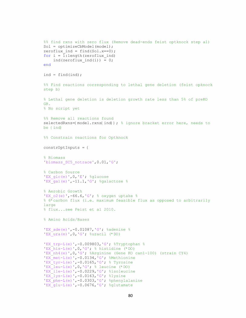
80

%% find rxns with zero flux (Remove dead-ends feist optknock step a1) Sol = optimizeCbModel(model); zeroflux_ind = find(Sol.x==0); for i = 1:length(zeroflux_ind) ind(zeroflux_ind(i)) = 0; end

ind = find(ind);

%% Find reactions corresponding to lethal gene deletion (feist opknock

step b)

% Lethal gene deletion is deletion growth rate less than 5% of preKO

GR. % No script yet

%% Remove all reactions found selectedRxns={model.rxns{ind}}; % ignore bracket error here, needs to

be {ind}

%% Constrain reactions for Optknock

constrOptInputs = {

% Biomass 'biomass_SC5_notrace',0.01,'G';

% Carbon Source 'EX_glc(e)',0,'E'; %glucose 'EX_gal(e)',-11.1,'G'; %galactose %

% Aerobic Growth 'EX_o2(e)',-66.6,'G'; % oxygen uptake % % 6*carbon flux (i.e. maximum feasible flux as opposed to arbitrarily

large % flux...see Feist et al 2010.

% Amino Acids/Bases

'EX_ade(e)',-0.01087,'G'; %adenine % 'EX_ura(e)',0,'G'; %uracil (*DO)

'EX_trp-L(e)',-0.009803,'G'; %Tryptophan % 'EX_his-L(e)',0,'G'; % histidine (*DO) 'EX_nh4(e)',0,'G'; %Arginine (Gene KO can1-100) (strain CY4) 'EX_met-L(e)',-0.0134,'G'; %Methionine 'EX_tyr-L(e)',-0.0165,'G'; % Tyrosine 'EX_leu-L(e)',0,'G'; % leucine (*DO) 'EX_ile-L(e)',-0.0229,'G'; %isoleucine 'EX_lys-L(e)',-0.0163,'G'; %lysine 'EX_phe-L(e)',-0.0303,'G'; %phenylalanine 'EX_glu-L(e)',-0.0676,'G'; %glutamate

81

'EX_asp-L(e)',-0.0746,'G'; %aspartic acid 'EX_val-L(e)',-0.128,'G'; %valine 'EX_thr-L(e)',-0.168,'G'; %threonine 'EX_ser-L(e)',-0.381,'G'; %serine % Compounds 'EX_nh4(e)',-7.58,'G'; %ammonium 'EX_so4(e)',-4.22,'G'; %sulfate 'EX_k(e)',-0.797,'G'; %potassium 'EX_pi(e)',-0.711,'G'; %phosphate 'EX_btn(e)',-8.2*10^-6,'G'; %biotin 'EX_inost(e)',-0.00556,'G'; %inositol 'EX_4abz(e)',-0.000146,'G'; %4-aminobenzoic acid 'EX_thm(e)',-0.000133,'G'; %thiamin 'EX_fe2(e)',-0.000123,'G'; % Iron (assuming fe3fe2) 'EX_na1(e)',-0.1711,'G'; % Sodium Ions 'ATPM',1,'E'; % ATP Maintenance

% please note that GRTT is NOT part of the media but a rxn constraint 'GRTT',.1,'G'; % GRTT min (added 7-23) };

% Must set at least two rxns here because optKnock is poorly written for i = 1:length(constrOptInputs) constrOpt.rxnList{i}=constrOptInputs{i,1}; constrOpt.values(i)=constrOptInputs{i,2}; constrOpt.sense(i)= constrOptInputs{i,3}; %G = greater %E is equal to;

L is for less than end

%% Options for optKnock (>>SET TARGET RXN and Number of KOs here<<<) options.targetRxn = 'GRTT'; options.vMax=120; %Set bound to feasible value instead of 'arbitrarily

large' i.e. 1000, 80 is 6*the carbon-6 source flux in case all flux

goes through 1 carbon compounds (feist optknock step a2) options.numDel =2; options.numDelSense = 'L';

%% Solve OptKnock disp('OptKnock Starts') optKnockSol = OptKnock(model, selectedRxns, options, constrOpt, [],

'true'); disp(['Optknock objective = ' num2str(optKnockSol.obj)]) disp(['OptKnock Growth rate =' num2str(optKnockSol.fluxes(1))])

%% Pre KO FBA tol = 1e-7; premodelKO = model; targetRxn=options.targetRxn; preKOsol = optimizeCbModel(model); pregrowthRate = preKOsol.f; disp(['preKO growth rate = ' num2str(preKOsol.f)]) targrxnind = find(strcmp(model.rxns,options.targetRxn)); disp(['preKO target rxn flux = ' num2str(preKOsol.x(targrxnind))]);

if (preKOsol.stat == 1) % Max & min production of the metabolite at the optimal growth rate

82

grRounded = floor(preKOsol.f/tol)*tol; premodelKO =

changeRxnBounds(premodelKO,premodelKO.rxns(premodelKO.c==1),grRounded,'

l'); premodelKO = changeObjective(premodelKO,targetRxn); presolMax = optimizeCbModel(premodelKO,'max'); presolMin = optimizeCbModel(premodelKO,'min'); premaxProd = presolMax.f; preminProd = presolMin.f; else premaxProd = 0; preminProd = 0; end

%% Test optKnock Solution %b stands for both lower and upper bound

tol = 1e-7; deletions = optKnockSol.rxnList; nDel = length(deletions); modelKO = model; targetRxn=options.targetRxn; for i = 1:nDel modelKO = changeRxnBounds(modelKO,deletions{i},0,'b'); end % Calculate optimal growth rate postKOsol = optimizeCbModel(modelKO); growthRate = postKOsol.f;

if (postKOsol.stat == 1) % Max & min production of the metabolite at the optimal growth rate grRounded = floor(postKOsol.f/tol)*tol; modelKO =

changeRxnBounds(modelKO,modelKO.rxns(modelKO.c==1),grRounded,'l'); modelKO = changeObjective(modelKO,targetRxn); solMax = optimizeCbModel(modelKO,'max'); solMin = optimizeCbModel(modelKO,'min'); maxProd = solMax.f; minProd = solMin.f; else maxProd = 0; minProd = 0; end

disp(['postKO growth rate = ' num2str(postKOsol.f)]) targrxnind = find(strcmp(model.rxns,options.targetRxn)); disp(['postKO target rxn flux FBA = '

num2str(postKOsol.x(targrxnind))]); disp(['preKO solmax target rxn flux = ' num2str(premaxProd)]); disp(['preKO solmin target rxn flux = ' num2str(preminProd)]); disp(['postKO solmax target rxn flux = ' num2str(maxProd)]); disp(['postKO solmin target rxn flux = ' num2str(minProd)]);

%% Script Written by Joseph Johnnie, Matt Conway, and Ashish Misra

Documents

ABSTRACT Title of Document: A SYSTEMS ENGINEERING ...austin/RecentGraduates/MSSE-Johnnie2011.pdf · A SYSTEMS ENGINEERING FRAMEWORK FOR METABOLIC ENGINEERING EXPERIMENTS By Joseph