Embed Size (px)
Citation preview
ABSTRACT
Title of dissertation: EXPRESSING PREFERENCES WITHPRICE-VECTOR AGENTS INCOMBINATORIAL AUCTIONS
Robert W. Day, Doctor of Philosophy, 2004
Dissertation directed by: Professor Subramanian RaghavanDecision and Information Technologies Department,The Robert H. Smith School of Business
In this work, we investigate two combinatorial auction formats in which
each bidding bidder may be represented by a collection of unit-demand or price-
vector agents. In the first model, bidder preferences are aggregated in a Bid Table,
through which a bidder in a combinatorial auction may express several forms of
subadditive preferences. We show that the gross substitutes property holds for this
model, and design a large-scale combinatorial auction using bid tables as a demand
revelation stage, determining linear price signals for later stages. The constraints of
this model coincide naturally with the restrictions of recently proposed FAA landing-
slot auctions, and we provide a slot auction design based on this model.
In a second model, we explore the more complex behavior possible when
each bidder’s collection of price-vector agents coordinate based on a bidder-specified
ordering of the auction items. With this coordination each bidder is able to convey
a rich set of preferences, including the ability to express both superadditive and
subadditive bundle synergies (i.e., substitutes and complements). The instructions
for this collection of agents are tabulated in a lower-triangular Matrix Bid, and we
compare the use of matrix bids to other compact techniques for writing down a wide
variety of bidding information. We show that the winner determination problem for
this Matrix Bid Auction is NP-hard, provide results from a series of computational
experiments, and develop IP techniques for improving run time.
In addition to the results on price-vector agents, bid tables, and matrix bid-
ding, we present a new technique for achieving bidder-Pareto-optimal core outcomes
in a sealed-bid combinatorial auction. The key idea of this iterative procedure is the
formulation of the separation problem for core constraints at an arbitrary point in
winner payment space.
EXPRESSING PREFERENCES WITH PRICE-VECTOR AGENTS INCOMBINATORIAL AUCTIONS
by
Robert W. Day
Dissertation submitted to the Faculty of the Graduate School of theUniversity of Maryland, College Park in partial fulfillment
of the requirements for the degree ofDoctor of Philosophy
2004
Advisory Committee:
Professor Subramanian Raghavan, ChairProfessor Michael BallProfessor Peter CramtonProfessor Bruce GoldenProfessor Dianne O’Leary

c©Copyright by
Robert W. Day
2004

ACKNOWLEDGMENTS
For my training in the mathematics of optimization, I thank Steven Gabriel,
Saul Gass, Bruce Golden, and Raghu Raghavan. Their treatment of the subject was
so exciting and well presented that I couldn’t help but become a student of the field.
For their courses on game theory, auctions and matching, I thank Larry
Ausubel and Peter Cramton. I feel greatly privileged to have learned from such
renowned and knowledgeable members of the field.
For his thorough review of an early draft, his ongoing interest in our research,
and for suggesting the example presented in §4.5, I thank Anand Anandalingam.
For his helpful comments and guidance, particularly in relation to the airport
application, I thank Michael Ball.
For her generous participation on the dissertation committee and careful
review of the dissertation, I thank Dianne O’Leary.
For its ongoing support of our research on “Rapid Response Electronic Mar-
kets for Time-Sensitive Goods” through NSF grant DMI-0205489, I thank the Na-
tional Science Foundation.
ii
For helpful comments and the sharing of ideas, through correspondence and
otherwise, I thank Wedad Elmaghraby, Karla Hoffman, David Parkes, and Michael
Rothkopf.
And most of all, for his guidance, support, enthusiasm and insight, I thank
my advisor Raghu Raghavan. He could not be more encouraging, respectful, or
enjoyable to work with. It has been a true pleasure.
iii
Contents
List of Figures vi
List of Abbreviations viii
Chapter 1. Introduction 1
Chapter 2. Auction Literature 13
2.1. Auction Applications 15
2.2. Auction Theory 26
Chapter 3. Bid Table Auctions 51
3.1. Assignment Preferences and the Gross Substitutes Property 54
3.2. VCG Bid Table Auction Implementations 66
3.3. Dynamic Bid Table Auctions 70
Chapter 4. A Three-Stage Auction for Airport Landing Slots 84
4.1. Auctioning Landing Slots 85
4.2. Schedule Auction Framework 89
4.3. Package Bidding and Probing 101
4.4. The Threshold Problem, the Free-Rider Problem and Efficiency 107
iv
4.5. Example of a Schedule Auction for Airport Landing Slots 112
Chapter 5. Generation and Selection of Core Outcomes 133
5.1. Core Constraint Generation 136
5.2. Examples and Comparison to the MiniMax Rule 147
5.3. Remarks on Core Constraint Generation 154
Chapter 6. Matrix Bidding 157
6.1. Interpreting a Matrix Bid 158
6.2. Integer Programming Formulation of Winner Determination 164
6.3. Preference Expression using Matrix Bids 171
Chapter 7. Computational Experiments for Matrix Bidding 199
7.1. Computational Procedure 201
7.2. Experiments with Simulated Data 216
Chapter 8. Conclusions 228
References 236
v

LIST OF FIGURES
Figure 1.1 A Bid Table 7
Figure 1.2 A Matrix Bid 10
Figure 2.1 Market settings for auctions 28
Figure 2.2 Auction design components 34
Figure 3.1 Assignment Preferences in a Bid Table 57
Figure 3.2 Preferences that do not fit in a Bid Table 64
Figure 3.3 A Bid Table Auction for which VCG payments are lower
than in any Walrasian equilibrium 66
Figure 4.1 Outline of the Schedule Auction 90
Figure 4.2 A Bid Table for landing slots 91
Figure 4.3 An auction for airport time slots: Stage I 116
Figure 4.4 Bundle probing in Stage II, assuming myopic best response 123
Figure 4.5 Results for all Stages, assuming myopic best response
in Stage II 126
Figure 4.6 Bundle probing in Stage II, assuming forthcoming bidders 130
vi
Figure 4.7 Results for all Stages, assuming forthcoming bidders
in Stage II 131
Figure 5.1 The Core Constraint Generation Algorithm 147
Figure 5.2 An auction for which threshold payments do not
minimize total payments 148
Figure 5.3 Comparison of Core Constraint Generation
to proxy methods 153
Figure 6.1 Assignment network for a Matrix Bid Auction 158
Figure 6.2 A grocery-list Matrix Bid 192
Figure 6.3 Matrix Bids for spectrum licenses 193
Figure 7.1 A nested k-of Matrix Bid 219
Figure 7.2 Average run time for winner determination 222
Figure 7.3 Percentage of LPs solving to integral optimality
vs. number of items 224
Figure 7.4 Worst case run time vs. number of matrix bids 225
Figure 7.5 Worst case run time vs. number of items 226
vii
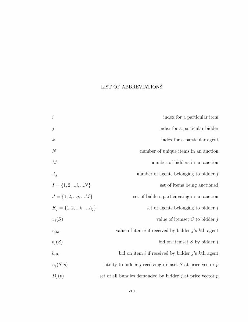
LIST OF ABBREVIATIONS
i index for a particular item
j index for a particular bidder
k index for a particular agent
N number of unique items in an auction
M number of bidders in an auction
Aj number of agents belonging to bidder j
I = {1, 2, ...i, ...N} set of items being auctioned
J = {1, 2, ...j, ...M} set of bidders participating in an auction
Kj = {1, 2, ...k, ...Aj} set of agents belonging to bidder j
vj(S) value of itemset S to bidder j
vijk value of item i if received by bidder j’s kth agent
bj(S) bid on itemset S by bidder j
bijk bid on item i if received by bidder j’s kth agent
uj(S, p) utility to bidder j receiving itemset S at price vector p
Dj(p) set of all bundles demanded by bidder j at price vector p
viii

i → j, k item i is awarded to bidder j’s kthagent in the selected efficient allocation
πj payment made by bidder j
W the set of winning bidders
πt a vector of payments for j ∈ W at iteration t
zC(πt) the coalitional value for C relative to payments πt
MBA a Matrix Bid Auction
∗ a significantly large negative number
ix

CHAPTER 1
Introduction
Auctions have long been used as a mechanism to allocate and determine a
price or competitive value for scarce resources. In the familiar English auction, an
auctioneer calls out prices on a single item or lot while bidders signal their willingness
to pay the current price until a single bidder remains, the winner of the item. This
mechanism arrives at an outcome that is efficient (the item for sale is given to the
bidder who values it the most) and the payment made is just enough to beat the
closest competitor. In addition, this simple auction has the desirable properties of
demand-revelation (the bidders get to learn about the preferences of other bidders
over the course of the auction), privacy-preservation (the winner never tells the
highest amount she is willing to pay) and incentive-compatibility (the best strategy
for each bidder is honest revelation; she stays in the auction until her true valuation
is met.) Krishna [34], for example, outlines these and other basic properties of
single-item auctions.
The situation becomes more difficult when the seller wishes to sell several
items at once. A bidder may perceive some items to be complements and others to be
substitutes and will face difficulties participating in several English auctions (or other
1

single-item auctions). For example, if a bidder perceives some collection of items to
be substitutes then it is difficult to know which single-item auction to compete in
to win just one item. On the other hand, when the items are complements a series
of single-item auctions forces the bidder to face an exposure problem; a bidder must
win an auction for the first item without knowing whether or not she will be able to
win the auction for the second item, and so forth. The presence of substitutabilities
and complementarities (which we will collectively call synergies) make it impossible
to guarantee an efficient auction outcome from a series of single-item auctions. This
difficulty has motivated the development of combinatorial auctions in which items
are awarded and bidder preferences are expressed over combinations or sets of items.
Given a set I = {1, 2, ...i, ...N} of N unique indivisible items, each bidder
j ∈ J = {1, 2, ...j, ...M} in a general combinatorial auction can be modeled by a
value function vj : 2I → R and a bidding function bj : 2I → R. To make precise the
notion of synergy, the primary motivation for the use of combinatorial auctions, we
adopt the following definition of the synergy perceived by bidder j on set S ⊆ I:
σj(S) = vj(S) −∑
i∈S
vj({i})
If synergy is positive, the bundle contains complements, if negative, mostly sub-
stitutes (as perceived by bidder j). As an adjectival alternative, we may refer to
2

preferences as subadditive, additive, or superadditive when bundle preferences expe-
rience negative, zero, or positive synergy, respectively.
This definition of synergy emphasizes the importance of both positive and
negative synergy which should both be considered in the design of a combinatorial
auction. If negative synergy is ignored (because, perhaps, the immediate benefits
to the auctioneer are not as obvious), bidders will feel the need to reduce their bids
because of exposure to the possibility of receiving substitute items at too high a
price, potentially leading to lost auction revenue. The presence of nonzero synergy
motivates an auction format in which each bidder discloses some bidding function
bj over bundles, and the auctioneer solves a combinatorial optimization problem to
find an allocation maximizing total bid revenue. This general winner-determination
problem can be formulated as an Integer Program (IP), with binary variables xj(S)
that equal 1 if and only if bidder j is awarded bundle S ⊆ I:
max∑
j∈J
∑
S⊆I
bj(S) · xj(S)(GWD)
subject to∑
S⊇{i}
∑
j∈J
xj(S) ≤ 1, ∀i ∈ I(1.1)
∑
S⊆I
xj(S) ≤ 1, ∀j ∈ J(1.2)
xj(S) ∈ {0, 1}, ∀S ⊆ I, ∀j ∈ J(1.3)
3
Constraints (1.1) ensure that each item is assigned to at most one bidder, while
constraint set (1.2) prevents the auctioneer from accepting multiple bids from the
same bidder.
It is well known in auction theory that a set of Vickrey-Clark-Groves (VCG)
prices may be computed that ensure each bidder will find it in her best interest
to bid truthfully, a property known as incentive compatibility [68][13][25]. This is
accomplished by computing a discount for each winning bidder by re-solving GWD
with that bidder removed. The VCG discount for bidder j is equal to the difference
between the objective value of GWD with all bidders and the objective value of
GWD with bidder j removed. If payments are assigned to winning bundles so as to
ensure truthful-revelation (i.e., if the VCG prices are used) then bidders will submit
bids bj = vj ∀j ∈ J and the optimal outcome to GWD is efficient.
Despite its beauty and simplicity, this approach has not been widely im-
plemented for several reasons. VCG mechanisms are susceptible to collusion and
false-name (or shill) bidding and do not necessarily generate enough revenue for the
outcome to be considered stable (in the sense of a core equilibrium). The general
winner determination problem (as formulated in GWD or otherwise) is NP-hard;
thus we cannot guarantee speedy (i.e., polynomial-time) convergence of an algo-
rithm for its solution except for very small problems. Further, the mechanism for
preference-revelation is direct: each bidder directly specifies a bid on every bundle.
4
This approach does not allow for demand-revelation; a bidder must write down prices
for all bundles without knowing what prices her competitor’s will name, despite the
fact the true value a bidder is willing to pay may be dependent on such information.
Privacy preservation is also compromised; the auctioneer knows the true valuations
of the winning bidders even though they pay less than the full amount. Finally, the
direct revelation of preferences may be exhausting for the bidder; evaluating each of
the 2N − 1 nonempty bundles of items will be impractical for more than just a few
items.
Several approaches have been suggested in the literature for conducting a
combinatorial auction that regains some of the desirable properties of the English
auction that are lost in a sealed-bid VCG implementation of GWD. We discuss a
number of these approaches and their relationship to our own work in Chapter 2.
Given the exponential data requirement to express preferences on every bundle and
the arbitrary nature of the restricted subset approach (discussed in §2.2.4) there is no
consensus in the literature on a single best combinatorial auction structure. Instead,
we pursue specialized algorithms and mechanisms tailored to specific markets or
bidder profiles.
In this dissertation, we concentrate on the exponential bundles problem of
combinatorial auctions and investigate new compact methods for a bidder to write
5
down bid information as an alternative to assigning a price to every bundle explic-
itly. Both of the approaches for preference elicitation explored here make use of the
concept of a price-vector agent. Each agent can be described as a fictional entity
representing some portion of the preferences of a particular bidder. A price-vector
agent is assigned a vector of prices (a monetary amount for each of the items in the
auction) and “participates” in the auction based on these prices. An agent receiving
a particular item pays at most the price vector component associated with that item.
Throughout we assume that each price-vector agent is a unit-demand agent; each
agent may receive at most one item. This clarifies the role of the price-vector agent
in economic terms: Each agent treats all items as perfect substitutes. Expression of
preferences using price-vector agents encourages each bidder to decompose his pref-
erences into collections of substitutable items and to dedicate one or several agents
to this collection depending on the level of substitutability (pure versus partial).
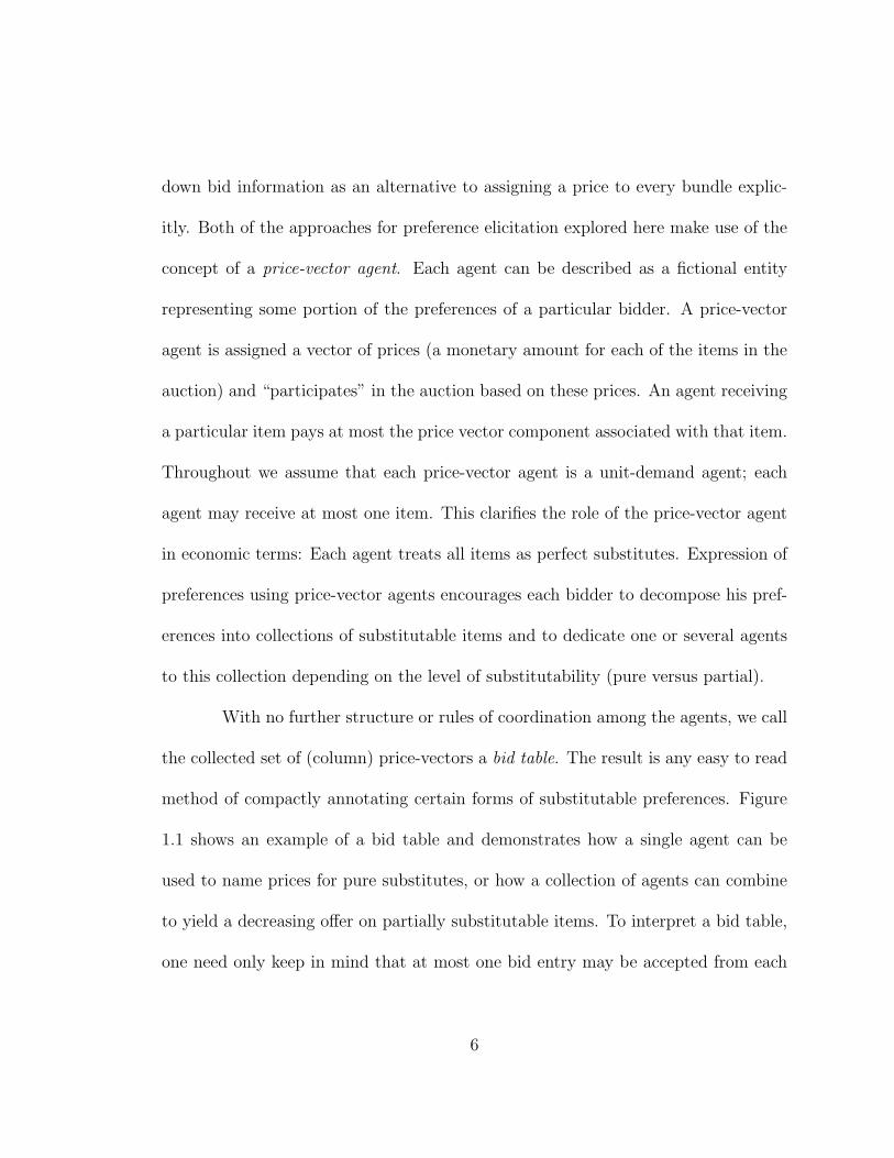
With no further structure or rules of coordination among the agents, we call
the collected set of (column) price-vectors a bid table. The result is any easy to read
method of compactly annotating certain forms of substitutable preferences. Figure
1.1 shows an example of a bid table and demonstrates how a single agent can be
used to name prices for pure substitutes, or how a collection of agents can combine
to yield a decreasing offer on partially substitutable items. To interpret a bid table,
one need only keep in mind that at most one bid entry may be accepted from each
6

Figure 1.1. A Bid Table
pure substitute A1
pure substitute A2
pure substitute A3
partial substitute B1
partial substitute B2
partial substitute B3
∣
∣
∣
∣
∣
∣
∣
∣
∣
∣
∣
∣
∣
agent 1 agent 2 agent 3 agent 415 0 0 016 0 0 017 0 0 00 23 18 120 20 16 100 19 15 9
∣
∣
∣
∣
∣
∣
∣
∣
∣
∣
∣
∣
∣
row, and at most one from each column. We see therefore that in the example of
Figure 1.1 that items A1, A2, and A3 are indeed pure substitutes, because at most
one can be purchased at a positive price. Similarly, if the bidder of this example
receives item B1 priced at 23, she cannot also receive (for example) item B2 at a
price of 20. If item B2 is assigned to the bidder, the revenue maximizing auctioneer
would be forced to accept a lower price from another agent of that bidder. In this
case the auctioneer would charge 16 for B2 rather than 20, verifying the partial
substitutability; B2 is worth less if taken with B1.
In Chapter 3, we show that the set of preferences expressible in bid tables are
properly contained in the set of preferences satisfying the gross substitutes property,
connecting this theory to the economic literature on restricted preferences. We may
then apply a theoretical result of Ausubel and Milgrom to elucidate a strength of
the Bid Table Auction: a VCG mechanism may be used with no possibility of dis-
ruption from false-name bidding or joint deviation by losing bidders, properties not
satisfied for a VCG mechanism in general. Despite this strength and the connection
7
to applications in which bidders determine bundle value via optimization over an
assignment network, the limitations presented by the gross substitutes property are
indeed great. In particular, no superadditive or complementary preferences may be
expressed.
The dissertation next divides in two directions, each concerning a different
method for the expression of preferences for complementary bundles in the price-
vector agent context. In Chapter 4, we show how a Bid Table Auction may be
incorporated as a demand revelation phase in a three-stage hybrid auction. We
demonstrate how supporting linear prices are extracted from the linear program-
ming (LP) dual of the winner determination optimization, and how they may be
used as signals of competitive activity and as eligibility requirements. The use of
bid tables for initial demand revelation allows for both ease of submission and for
reduced bid exposure relative to a Simultaneous Ascending Auction (SAA) filling
the same role in a hybrid auction. The reduction of exposure allows a new en-
trant to simultaneously compete in several markets without the danger of exceeding
her capacity for items. We develop our hybrid auction incorporating bid tables in
the context of recently proposed Federal Aviation Administration (FAA) landing-
slot auctions. The comprehensive design is summarized as follows: a linear price
demand-revelation stage using bid tables, a demand-revelation stage with bundle
8
prices, and a sealed-bid final stage achieving efficiency (relative to the submissions)
and bidder-Pareto-optimal core prices.
The computation of bidder-Pareto-optimal core prices via the separation
and generation of core constraints is treated independently in Chapter 5, due to its
applicability in other sealed-bid auction contexts. Among this material we consider
the selection of a bidder-Pareto-optimal core outcome among all Pareto efficient core
points, a matter that is currently unsettled in the literature. In particular, we argue
in favor of a core outcome that minimizes the total payments made by all bidders and
show that the minimax techniques explored by Parkes [54] do not necessarily achieve
this outcome. In addition, we show how a simple perturbation technique allows us
to choose the most equitable outcome when there are several that minimize total
payments.
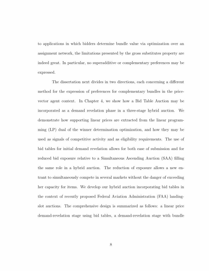
In Chapter 6 and Chapter 7, we explore the use of price-vector agents with
additional constraints applied to enforce a simple form of cooperation among the
agents belonging to an individual bidder. The bidder in this context submits a
ranking or strict ordering of the items in the auction, while the previously permutable
price-vector agents are each given a defined rank. Each price loaded into an agent
then represents what that agent is willing to pay for a particular item, given that
the superior agent (the one coming just before this agent in the ranking) receives
a superior item (any coming earlier in the ranking). We show that this “pecking
9
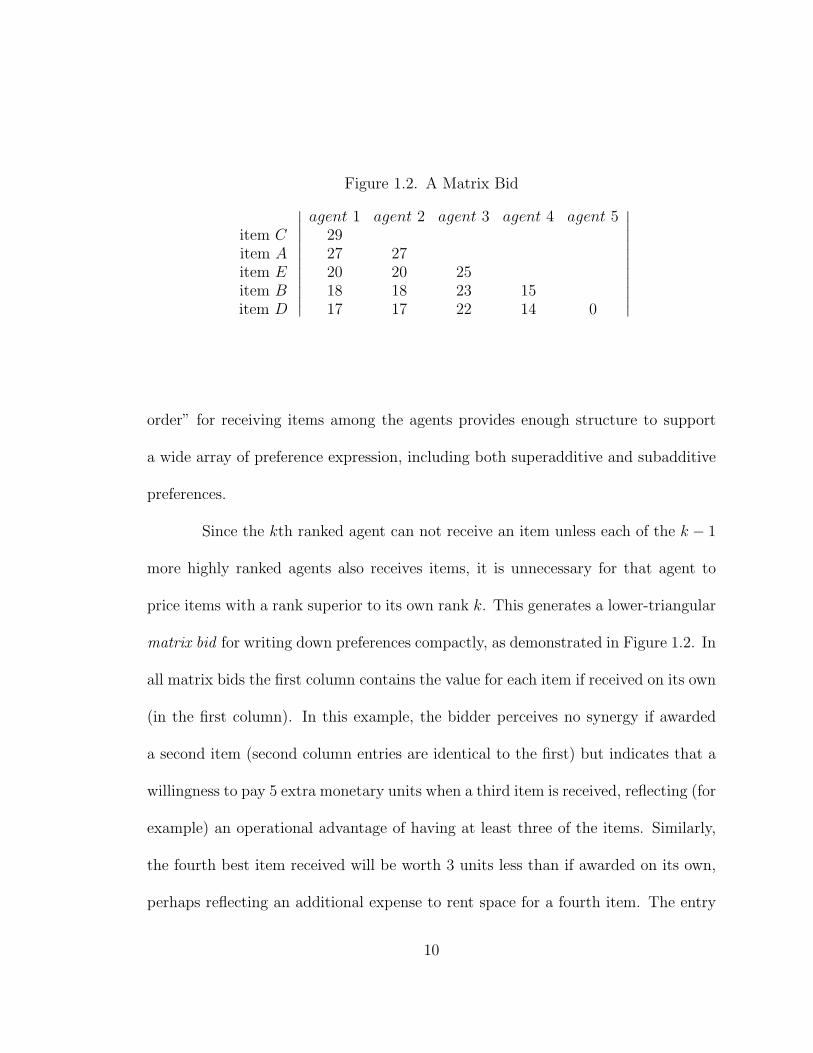
Figure 1.2. A Matrix Bid
item Citem Aitem Eitem Bitem D
∣
∣
∣
∣
∣
∣
∣
∣
∣
∣
∣
agent 1 agent 2 agent 3 agent 4 agent 52927 2720 20 2518 18 23 1517 17 22 14 0
∣
∣
∣
∣
∣
∣
∣
∣
∣
∣
∣
order” for receiving items among the agents provides enough structure to support
a wide array of preference expression, including both superadditive and subadditive
preferences.
Since the kth ranked agent can not receive an item unless each of the k − 1
more highly ranked agents also receives items, it is unnecessary for that agent to
price items with a rank superior to its own rank k. This generates a lower-triangular
matrix bid for writing down preferences compactly, as demonstrated in Figure 1.2. In
all matrix bids the first column contains the value for each item if received on its own
(in the first column). In this example, the bidder perceives no synergy if awarded
a second item (second column entries are identical to the first) but indicates that a
willingness to pay 5 extra monetary units when a third item is received, reflecting (for
example) an operational advantage of having at least three of the items. Similarly,
the fourth best item received will be worth 3 units less than if awarded on its own,
perhaps reflecting an additional expense to rent space for a fourth item. The entry
10
of zero in the fifth column indicates that five items is beyond this bidder’s capacity
to consume; no additional payment will be given for a fifth item.
This example gives just a glimpse of the expressability possible with a single
matrix bid. In Chapter 6 we explore the basic properties of matrix bidding and pro-
vide examples of several types of possible expressions. Motivated by other logically
structured “bid languages” presented in the literature, we show that an individual
matrix bid has the ability to contain any of the proposed “atomic” statements of
preference used to build compound sentences of preference. Further, several of these
bid atoms may be contained in a single matrix bid, which may also be supplemented
with “salvage value” bids on any or all items. This allows the bidder to make a
positive incremental offer on any item as an add-on to a specified package bid (of
any type) whenever the additional items will bring positive value, and provides the
ability to do so within the same atomic statement of preference. We show that a
logical bid language with matrix bids as atoms is as expressive as the most robust
logical language presented in the literature [9], and relative to that language may
often require less atoms and less symbols to represent a given set of preferences.
We show that the winner-determination problem for a matrix bid auction is
NP-hard. In Chapter 7 we present computational findings on our ability to solve
instances of this problem, including instances with as many as 50 items and 100
11
matrix bids. In this development we uncover some interesting properties and de-
velop heuristics based on our experience dealing with fractional solutions to the LP
relaxation of the IP winner determination problem. Among these techniques are the
recognition of a class of cover-like inequalities with a heuristic for the correspond-
ing separation problem, and an objective perturbation technique designed to favor
integral extreme points over fractional solutions with the same objective value (an
occurrence which was not rare in our initial computations).
Before describing our own results in greater depth, we first present a review
of recent auction literature in Chapter 2, paying particular attention to research with
an Operations Research (OR) flavor.
12

CHAPTER 2
Auction Literature
Research on auctions has been developed in the Economics literature through
the study of strategic games [68] and in the OR literature as constrained optimiza-
tion since the mid 20th century [24]. More recently, there has been a great deal of
intellectual cross-pollination from Management Science, Information Systems, and
Computer Science in an attempt to develop new electronic markets providing better
economic outcomes through centralized computational decision making. The com-
putational difficulties presented by these markets are not readily untied from their
economic context, making it difficult to apply a purely algorithmic approach which
ignores strategic considerations. Conversely, the most general economic allocation
problems exhibit a level of computational complexity (NP-hardness) that requires
algorithmic expertise, making it difficult to attack these market design problems
from a purely economic standpoint. This is especially true if we consider a very
general definition of an auction:
Definition: An auction is a mechanism of information submission, together with
rules for assigning items and payments to participants based on this submitted in-
formation.
13

Since the OR discipline emphasizes the successful implementation of deci-
sion making technology in real-world situations, we begin with a quick survey of the
successful and growing applications of auction theory, keeping this general definition
in mind. The most widely recognized electronic auction is undoubtedly eBay and
similar electronic venues for commerce that may be described as mostly consumer-to-
consumer. The success of these markets demonstrates that the “electronic” services
(a web-based platform) provide added-value even when the “auction” structure is
simple (one-seller, one-item, simple bidding rules). Though several interesting av-
enues of research receive attention from these consumer-to-consumer settings, the
success and future of the OR approach to auctions seems to stem from the use of
auctions in business-to-business (B2B) commerce and government allocations, where
the value-added is derived from the ability of the auction mechanism itself to elicit
and process information, determining a more favorable outcome in a centralized mar-
ket. These auctions typically have a “combinatorial” component, in which bidders
may express how their preferences vary over combinations or bundles of items. This
quality at once promises to extract value from the auction decision mechanism, and
places the computational challenge for the mechanism at the very frontier of what
is possible through computational technique.
14
2.1. Auction Applications
2.1.1. Auctions and Governmental Allocation
From the perspective of applications, auction mechanisms first entered the OR
literature in the context of government controlled allocation problems. Throughout
this literature, auctions are proposed as a tool of deregulation. Rather than allowing
governmentally controlled resources to be distributed via political decision-making
criteria and regulatory control (typically an inefficient procedure), auctions provide
a market-based mechanism to allocate government property fairly. Before any such
paradigm shift can take place, researchers must first provide scientific evidence that
the auction mechanism will produce favorable outcomes, and that the auction can be
implemented smoothly and at a comfortable pace for all participants. The pursuit of
such evidence for governmental problems inaugurated the field as it is known today,
with the healthy mix of theory and implementation indicative of Management Science
and OR.
Rassenti, Smith, and Bulfin [59] pioneered this line of work in 1982 with
one of the first efforts to confront multi-item auction winner-determination prob-
lems with the computational techniques of Integer Programming (IP). In this work
they propose an auction mechanism for the allocation of airport time-slots and give
some of the first experimental verification (using test subjects) that the combinato-
rial auction paradigm can achieve more efficient outcomes than a non-combinatorial
15
mechanism. The auctions and corresponding winner-determination IPs are modest
in size, reflecting the difficulty and lack of scalability in solving these hard allocation
problems.
Ironically, though the airport time-slot application was one of the first pro-
posed for the use of combinatorial auctions, the FAA is only now beginning to con-
sider the use of auctions to control demand for landing/take-off slots. Ball, Donohue,
and Hoffman [6] provide a description of the necessary and desirable features in air-
port slot auction and provide the motivation for the airport landing-slot auction that
we develop in Chapter 4. A parallel and quite thorough investigation of the pros-and-
cons of airport-slot auctions in the European market is given by the consulting firm
dotEcon [21]. Both emphasize the economic benefits of an auction mechanism for
the allocation of landing-slots at congested airports, and advocate a combinatorial
auction implementation to achieve the desired results. Most recently, NEXTOR (the
National Center of Excellence for Aviation Operations Research) and the FAA have
sponsored two workshops ([48], [49]) exploring the use of auctions for congestion
control.
Another early influential work rooted in governmental applications is given
by the Adaptive User Selection Mechanism (AUSM) of Banks, Ledyard, and Porter
[7], proposed to allocate resources such as jobs on a super-computer or mission time
aboard a space station. Like Rassenti, Smith, and Bulfin [59], this paper began
16

to stir interest in auction research outside of Economics. Though published in an
economics journal, the work of Banks, Ledyard and Porter suggests that scheduling
and logistical problems (typically the bread and butter of the OR community) could
be handled by adapted auction mechanisms. Further, their approach was progres-
sive in the use of decentralized computation, shifting computational burden away
from the central decision making entity and to the bidding agents themselves. This
“agent-based” decision making has been a hot topic in several fields of research and
has strongly influenced the more recent auction literature of Kelly and Steinberg
[32], who connect this line of research to another government application: universal
telephone service obligations. These two works provide a great deal of motivation
for our three-stage hybrid auction described in Chapter 4. In particular, we borrow
their ideas for demand revelation through user-selected bundle offers, but attempt to
improve their methods by diminishing unnecessary computational searching and the
ability of bidders to “free-ride” on the revealed demand of others. A more thorough
comparison of our hybrid auction to the adaptive user selection technique is provided
in Chapter 4.
We note that Ausubel, Cramton, and Milgrom [4] also describe a hybrid
auction, the Clock-Proxy Auction, developed concurrently with this dissertation.
This auction consists of a demand revelation (clock) stage and a sealed-bid (proxy)
stage. In the clock stage bidders report their demand for items at the given prices,
17
and prices are adjusted upward until there is no excess demand. At the conclusion
of this stage, bidders submit bids for bundles of items to a computer proxy, and an
Ausubel-Milgrom [5] proxy auction follows, determining an allocation of packages
and the corresponding bidder payments.
Potential governmental applications for auctions abound, though the one
discussed most prominently in the literature seems to be auctions for the allocation
of personal communication spectrum licenses. The sellers of these licenses (such as
the Federal Communication Commission (FCC) in the United States) have no sig-
nificant costs to recover for each license granted, so that the value for such items
are determined almost exclusively through competition on the demand-side. More
importantly, because several licenses in the same frequency range must be acquired
to form a functioning communications network, the value that a particular telecom-
munications firm places on a given set of licenses is very heavily influenced by which
other licenses it has received. This property suggests that a series of single-item
auctions would not lead to an efficient outcome in this market and that a more com-
plex auction mechanism should be considered. In the FCC auction-design debate
of the early 1990’s, it was determined that a combinatorial or package bid auction
should not be considered since the general combinatorial auction winner determina-
tion problem was computationally intractable (i.e., NP-hard) (see [45]). The FCC
instead adopted the Simultaneous Ascending Auction (SAA) auction, which allows
18

for simultaneous price discovery without package bidding, foregoing the potential
benefits of package bidding due to its computational difficulty. The FCC reported
$32 billion in revenue using this approach in 32 auctions between 1994 and 2001 (see
[37]).
This underlying all-or-nothing assumption that a hard computational prob-
lem should either be handled completely or not all is antithetical to the OR approach
and has been challenged in this context. As the seminal work of Rothkopf, Pekec, and
Harstad [62] points out, many special cases of an NP-hard problem like the combi-
natorial auction winner determination problem can be solved efficiently, suggesting
several applications in which a combinatorial auction can be quickly implemented,
including special cases in which the size or type of bundles which may receive bids are
restricted without objection from the bidders. The debate surrounding the FCC’s
design problem helped introduce auction theory to the OR community as a set of
complex decision problems, open to heuristic techniques and algorithms tailored to
specific classes of instances. The flurry of research that followed paved the way for
the current landscape of auction implementation, in which B2B auctions take place
using market-specific structure and IP techniques, as discussed below. The FCC
seems to have accepted the possible benefits of such a paradigm shift, that a “par-
tial” or “restricted” combinatorial auction may be successfully implemented using
limited package bidding and IP solvers, as evidenced by the proposed (and serially
19
postponed) Spectrum Auction #31, discussed, for example, by Gunluk, Ladanyi,
and de Vries [28].
Many auctions are complicated by the complex way in which the items com-
bine to form valuable bundles, including auctions for spectrum licenses. A set of
spectrum licenses may have a combined value more than the sum of its parts if the
licenses geographically cover a particular large region such as the Eastern Seaboard
or if they cover a continuous frequency range in a particular region. Furthermore, it
may be difficult or unreasonable for the auctioneer to determine in advance which
bundles should be considered as valuable since this may vary from bidder to bidder.
It is precisely in this situation, where the items at auction have multiple attributes or
may be combined differently by different bidders, that the decision problem becomes
difficult and advanced combinatorial auction mechanisms become advantageous.
Though spectrum auctions and similarly complex markets dominate the
decision-science-type auction literature, auctions are commonly employed for several
other governmental allocation problems which receive less attention for their compu-
tational difficulty. The most important examples in this group include treasury-bill
and electricity auctions, where the auctioned items have fewer distinguishing char-
acteristics and demand can be expressed simply as quantities demanded of a few
simple types. Treasury-bills in particular are “commodity-like” and do not combine
in complicated ways to form valuable bundles, making advanced auction/decision
20
techniques unnecessary in terms of implementation, though the game-theoretic anal-
ysis of these markets may not be trivial (see the work of Ausubel and Cramton [3]).
It is, however, important that we include treasury auctions among the success stories
of government allocation auctions; these markets provide an excellent model for auc-
tioning several “commodity-like” items, especially in situations where diminishing
marginal returns dominate.
With spectrum auctions as an example of a market in which items com-
bine to form bundles in a complicated way, potentially benefitting from the use of
a combinatorial auction mechanism, and treasury auctions as an example where no
such complications arise, making combinatorial machinery unnecessary, deregulated
wholesale electricity markets seem to provide a middle ground. On one hand, the
items at auction (kilowatt-hours of electrical power supply) are very commodity like,
i.e., divisible (simplifying analysis and implementation) and deriving the majority
of their value intrinsically, rather than through synergy with other auction items.
On the other hand, some synergies do arise in the form of power generator start-
up and no-load costs, so that a “pure-commodity” approach may distort a bidding
power supplier’s ability to communicate true costs of production. This leaves a
bidder to either misrepresent her preferences on the side of caution, or to risk dis-
satisfaction with the results of the auction. The electricity market may therefore
be treated with a “tatonnement” procedure, familiar from the economics literature,
21
modified to handle the non-convexity imposed by the start-up and no-load costs.
Market Design, Inc. (www.market-design.com), an auctions consulting firm, has
successfully implemented such specialized “clock auctions” for the wholesale elec-
tricity markets in France and Alberta, Canada, and have consulted in regional U. S.
markets. (Cramton [14] provides details.) These regional U.S. markets, such as the
Pennsylvania-New-Jersey-Maryland (PJM) system, take a markedly OR approach
to electricity allocation, solving Mixed Integer Programs (MIPs) for daily electricity
dispatch. The possibility of a centralized restructuring of the U. S. energy market to
allocate and price electricity using sophisticated IP-type auction techniques is cur-
rently under investigation by the Federal Energy Regulatory Commission. O’Neill
et al. [51] describe this research.
2.1.2. Auctions and B2B Commerce
While the authorities on the government applications that motivated much of
the early combinatorial auction research were reluctant to implement the change to
a “package bidding” auction, pioneers of B2B e-commerce quickly recognized the
potential benefits of advanced auction techniques and began conducting “combina-
torial” auctions as a market intermediary in the mid-1990s. Today, several firms offer
auction consulting services, helping a firm conduct an auction for the procurement of
transportation lanes, raw materials and other services. Procurement auctions (with
22
a single buyer and several suppliers or sellers, also called reverse auctions) with at
least some combinatorial machinery have been conducted by CombineNet [40], IBM
[31], Logistics.com [43], Net Exchange [39], and Emptoris [67]. These B2B auctions
assure savings to the procurer through increased price competition and the ability to
constrain product quality, delivery-time, and other non-price attributes of the items
provided. Conversely, strategic, logistical, and scaling problems facing suppliers
are often alleviated with bundle bidding, which may allow expression of volume-
discounts, incompatible products/services, and complementary products/services.
In a typical procurement auction, the buyer initiates the auction by inviting
quotes from several competing suppliers for a particular set of services (or items).
In a combinatorial procurement auction the buyer often has the ability to place
other restrictions on the final allocation, such as a lower bound on the number of
sellers to ensure diversity and lack of dependence on a particular seller. Other ser-
vices may be unnecessary unless complementary services are also performed and a
buyer may express a need to have a certain subset of services all provided by the
same bidding supplier where necessary. On the other end, a supplier may express
interest in supplying services only when complementary services are also performed,
or may conversely express a desire to only provide a particular service if substitute
services are not performed. With this wide range of expressability over both sub-
stitutes and complements desirable for both buyers and sellers in the proposed set
23
of B2B applications, the optimization approach to winner determination seems to
dominate tatonnement models modified to accept combinatorial information in this
context. Indeed, much of the available literature on procurement auctions utilize
an IP approach, which is generally flexible enough to accept a wide range of logical
statements of preference.
This need for a fully flexible “bid language” is evident in the market for
transportation or shipping lanes, in which a buyer requests offers to ship various
loads across origin/destination pairs (shipping lanes). In traditional shipping lane
markets bidding shippers face uncertainty in the final bundles they receive, making
it difficult to forecast their own global shipping schedule, or to express how internal
constraints may effect their contractual decision making (e.g. “I can move shipment
A or shipment B but not both. Which one should I bid on?). Though the problem
becomes too large for IP techniques (and for bidders) when prices are submitted for
every possible bundle, it is well known that optimization problems like the winner-
determination problem are often more easily solved with the addition of constraints,
in this case corresponding to a priori restrictions of the types of bids which may be
submitted. Unfortunately, it is difficult to make a prior restrictions on the types of
bundles that may be bid on in a shipping lane auction, partly because some of the
factors determining the value of a bundle of shipping lanes for a particular shipper
may be exogenous to the auction at hand. For example, certain shipping lanes may
24
be complementary to pre-existing contractual obligations of the shipper; a shipper
would be especially eager to fill trucks that would otherwise be empty return-trips
under existing contracts. Because so many exogenous factors exist and vary from
shipper to shipper, a very general bid language seems necessary for this scenario.
IP approaches that add restrictions (cuts) only as bid information is received from
bidders seem particularly advantageous here.
Sears Logistics held the first large scale auction for shipping lanes using
“combined value” or package bids in the mid 1990s with the software support of Net
Exchange [39]. Their encouraging results suggest that satisfaction with the market
mechanism and efficiency may be increased on both sides of the market. Sears
Logistics (the procurer of shipping lanes in this case) reported savings of $25 million
(13%) in their first combined value auction, while shippers were able to eliminate
uncertainty and exposure to winning incompatible or incomplete sets of lanes. With
this success documented, it is not surprising that several other large corporations
decided to introduce the combinatorial auction paradigm for shipping; Logistics.com
reports the implementation of procurement auctions on behalf of Walmart Stores,
Compaq Computer Co., Staples Inc., The Limited Inc., and Kmart Corporation [43].
In addition, Elmaghraby and Keskinocak [22] provide a case study of a successful
shipping lane auction for Home Depot.
25
The acceptance of a combinatorial auction format using IP decision-making
techniques for transportation procurement should not be surprising. Internal supply-
chain and logistics decisions are often approached from the IP perspective, mak-
ing the use of IP software for community or market decisions a natural transition.
Though less apparent, procurement auctions are finding their way into more general
settings, though more reports of success stories may be necessary before they are
accepted on a large scale. Some notable success stories include those of CombineNet
who report 15% surplus gained by participants in procurement auctions for raw ma-
terials (such as coal and steel) and shipping lanes since 2001 [40]. In addition, IBM
has implemented several combinatorial procurement auctions for Mars, Inc., empha-
sizing that benefits accrue on both sides of the market (implying overall efficiency
gains) and that payback on Mars’ investment was less than a year [31]. In general,
experts advocate that a successful procurement auction may be conducted in mar-
kets with a relatively small static group of suppliers, and that mechanism design
should emphasize efficiency rather than procurer profits, so as to establish favorable
long term relationships. Parkes [55] supports this position.
2.2. Auction Theory
Several auctions have been studied and implemented for many years, the
English auction and its variants being the most familiar. In an English auction, an
item is to be sold (one at a time), but an accurate market price is unknown. In order
26
to determine a price that is satisfactory to both buyer and seller, an auctioneer names
successively higher prices, and bidders respond with their willingness to accept these
prices, or by dropping out of the auction. The auction concludes when only one
bidder is willing to pay the current price. This last bidder receives the item at the
price that is a single increment higher than the amount that the next highest bidder
is willing to pay. This simple auction is both incentive compatible (truth-telling is
the best strategy) and efficient (the item goes to the bidder who values it the most).
Other long-standing auction formats for a single item include the Dutch
auction, in which the price descends until the first bidder bids and wins the item,
and the sealed-bid auction, in which bidders each submit a price for the item in
question, with the highest bid winning. Auction theorists show that under mild
assumptions, the same strategic behavior should be expected for the Dutch and
“first-price” sealed-bid auctions, in which the highest bidder pays the amount of
her bid. The “second-price” sealed-bid auction (a sealed-bid auction together with
the condition that the highest bidder wins the item at the price specified by the
second-highest bidder) displays incentive-compatibility. Under an assumption that
a bidder’s valuation does not depend on the valuation information revealed by her
opponents, the second-price sealed-bid auction produces the same outcome as the
English auction (see [34]).
27

Figure 2.1. Market Settings For Auctions
Number of Participants Types of Items Number of Items Differentiation
one Seller, many Buyers
one Buyer, many Sellers
many Buyers and Sellers
Divisible
Discrete
Single-Item
Multiple-Items
Identical Items
Distinct Items
These observations on the equivalence of various auction outcomes, together
with the strategic analysis showing that a bidder has no ability to benefit from an
untruthful strategy in certain simple auctions, provide the “classical” basis of auction
theory. There are two major avenues of contemporary auction theory building on
these classical foundations. With a behavioral approach, many pursue more accurate
models of bidders to explain the differences between empirical data and theoretical
predictions. Others auction theorists design new auction formats for simultaneously
auctioning several items, like those proposed in the current work. The challenge of
this pursuit is to combine computational feasibility, economic efficiency, and strategic
lucidity in a multi-item auction format. Before introducing these research avenues in
greater depth, we must first make clear some underlying scenarios and terminology.
2.2.1. Market settings for auctions
Figure 2.1 illustrates the full array of market types for which auctions have been
studied. Almost any combination of selections from each column yields a different
type of market (the only exception being that the question of differentiation among
items has no meaning when only a single item is to be auctioned.) Together this
28

enumerates 18 different market settings to which auctions may potentially be applied.
Auctions with a single seller are often referred to as forward auctions, as this is the
most familiar format. An auction with single buyer and several sellers is usually
called a reverse auction, but is also known in the literature as a procurement auction.
Markets with many buyers and sellers have been called both exchanges and
double auctions. Since there is a large amount of literature concerning exchanges
(due to their importance in finance), it may be useful to make a distinction between
exchanges and double auctions. Based on current business practices, we propose
that an exchange should refer to an open market in which transactions have the
opportunity to occur at any time and require only the agreement of the transactors, as
in the stock market. A double auction, on the other hand, should refer to markets in
which all transactions are decided by a central information collecting entity, adhering
to our earlier definition of an auction.
In this dissertation. we maintain a forward auction setting as is common in
the literature. As we are interested in areas on the cutting edge of computational
difficulty, we focus on auctions for multiple, discrete items. In general we will assume
that each item is distinct or distinguishable from any other item.
29
2.2.2. Single-Item Auctions
Single-item auctions have been studied in economics as games of incomplete
information for over forty years [68], and may be considered well-understood. Spe-
cific topics of interest include several models for the auction of a discrete item with
varying assumptions on the behavior of bidders. These models vary according to the
amount of information available to each bidder, whether each bidder knows his own
valuation for certain or bases this value somewhat on what others think, and the
amount of affiliation or correlation among the values of bidders.
For example, the seeming equivalence in outcome between the English and
second-price auctions breaks down when bidders’ utility is governed by affiliated
signals (see [46]). In this circumstance the English auction has higher expected rev-
enue, because bidders in the English auction learn over the course of the auction and
can bid more competitively with better information. In the second-price auction, on
the other hand, lack of information about the value of the item induces conservative
bidding. The complete result for single-item auctions is that in terms of maximizing
auctioneer revenue, the English auction outperforms the second-price auction which
in turn outperforms the first-price auction. Again, Krishna [34] provides a good
overview of this fundamental material.
As noted above, similar results hold that the Dutch auction may be consid-
ered strategically equivalent to the first-price sealed-bid auction. This equivalence
30

is challenged, however, in new work by Carare and Rothkopf [11] who show that
slow Dutch auctions (in which the price drops slowly over the course of a few days
in an internet auction) may produce more revenue than the first-price auction (see
also [44]). As in several of recent papers which challenge long-standing principles
of auction theory, we see that the simplifying assumptions used in theoretical work
may lead to conclusions which no longer hold when the model is extended to describe
the real world more accurately. In the case of Carare and Rothkopf, we see that the
value of time must be included as a transaction cost in models of Dutch auctions,
and that failure to capture all costs in an auction model may skew a seller’s decision
making criteria when selecting a particular auction.
Other interesting new topics in the world of single-item auctions include
explaining the difference in equilibrium behavior between theoretical work and em-
pirical study. Indeed, real-life bidders do not behave as game theory suggests they
should, often not understanding the incentive implications of VCG pricing or the
need for proper conditional probabilities to mitigate the “winner’s curse”. Deltas
and Engelbrecht-Wiggans [18], and Ding et al. [20] provide a glimpse into the field
of behavioral economics and its intersection with auction theory. The former pro-
vides justification for the persistence of strategically naive behavior, while the latter
examines the effect of emotional factors (excitement and frustration) on bidder be-
havior and auction participation. In both cases the auction format is held to the
31
simple case of a single item in order to study bidders’ behavior, which may be very
complex despite the simple setting.
2.2.3. Multiple-Item Auctions
The study of multiple-item auctions (or multi-unit auctions) has received greater
attention than single-item auctions in recent years, and consequently represents a
greater portion of the auction literature reviewed here. Situations proposed for these
auctions include forward, reverse, and double auction settings for identical or distinct
items that are either discrete or divisible (i.e., all possibilities). Theorists usually
assume that results for forward auctions hold for reverse settings and use whichever
terminology is convenient for their proposed area of application. Even though many
results do apply generally, whether specific auction designs work better for different
numbers and types of market participants is territory that has been explored only
on an ad hoc basis.
Combinatorial auctions are multiple-item auctions for which bids may be
placed on packages of items, and are often referred to as auctions with package-
bidding. Neither term should be used to refer to multiple-item auctions in general,
since many important types of multiple-item auctions need not accept such bids.
The Simultaneous Ascending Auction long used by the FCC provides an example of
a format that is multi-unit but not combinatorial.
32
Combinatorial auctions may provide more beneficial outcomes when the
value of an item received by a bidder is determined heavily by the other items
received. Many applications have been proposed including electricity markets, equi-
ties trading, bandwidth auctions, transportation exchanges, pollution right auctions,
auctions for airport landing slots, supply chains, and auctions for carrier-of-last-resort
responsibilities for universal services [65]. As mentioned above, innovative vendors
already host a significant amount of B2B commerce using combinatorial auctions,
making the study and development of more specialized combinatorial auctions a
lucrative pursuit, despite the computational difficulties to bidders and auctioneers
alike.
Certain developments in the study of multi-unit auctions in general can
be attributed to economic reasoning similar to the results surrounding single-item
auctions. The behavior of models which extend these ideas to the case of distinct
items is less well understood. Much of the analysis attending multi-item multi-round
auctions rely heavily on assumptions of substitutability among the items being auc-
tioned. Complementarity of items is a widespread phenomenon in markets for which
multi-unit auctions are proposed, and the existence of superadditive prices (among
complements) is a strong reason for expecting that multi-unit auctions might produce
higher revenues than separate single-unit auctions. These strong substitutability as-
sumptions should therefore be treated with some suspicion.
33
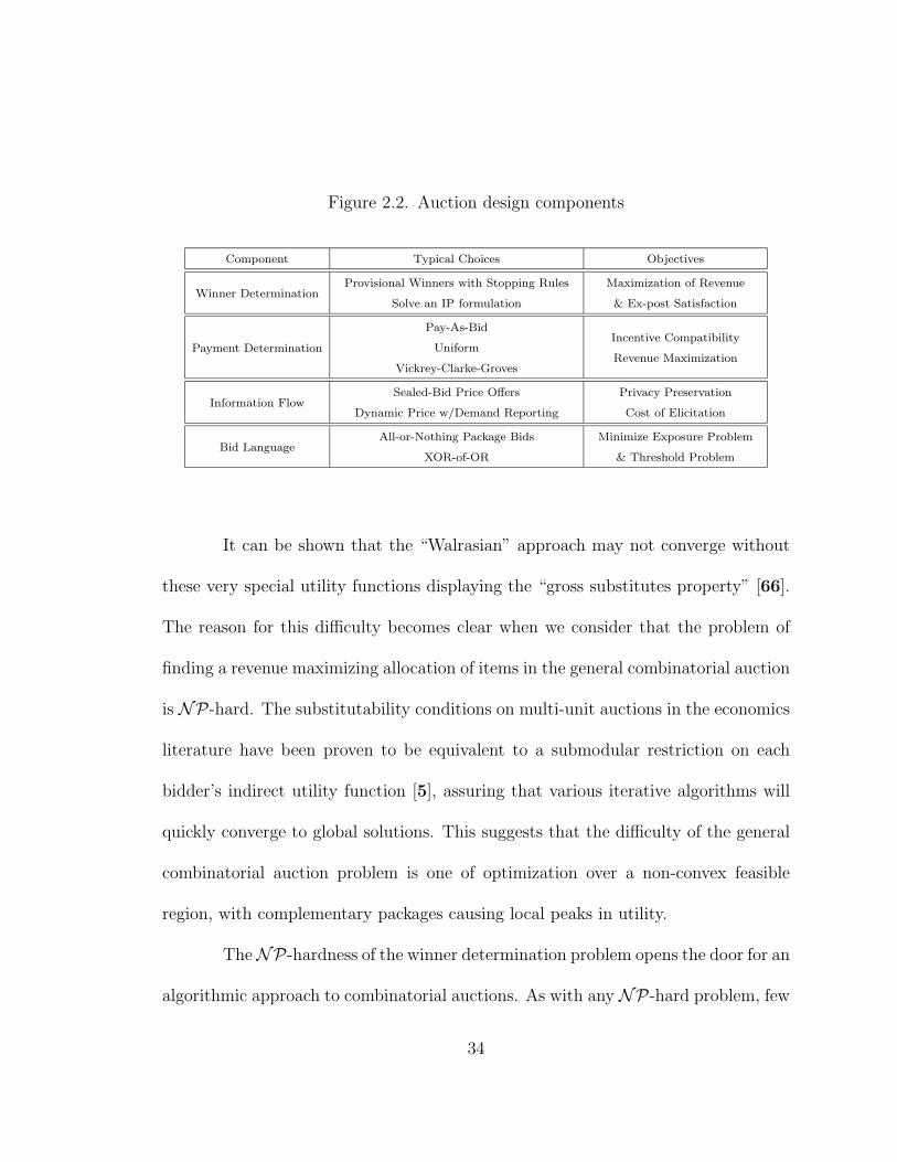
Figure 2.2. Auction design components
Component Typical Choices Objectives
Winner DeterminationProvisional Winners with Stopping Rules
Solve an IP formulation
Maximization of Revenue
& Ex-post Satisfaction
Payment Determination
Pay-As-Bid
Uniform
Vickrey-Clarke-Groves
Incentive Compatibility
Revenue Maximization
Information FlowSealed-Bid Price Offers
Dynamic Price w/Demand Reporting
Privacy Preservation
Cost of Elicitation
Bid LanguageAll-or-Nothing Package Bids
XOR-of-OR
Minimize Exposure Problem
& Threshold Problem
It can be shown that the “Walrasian” approach may not converge without
these very special utility functions displaying the “gross substitutes property” [66].
The reason for this difficulty becomes clear when we consider that the problem of
finding a revenue maximizing allocation of items in the general combinatorial auction
is NP-hard. The substitutability conditions on multi-unit auctions in the economics
literature have been proven to be equivalent to a submodular restriction on each
bidder’s indirect utility function [5], assuring that various iterative algorithms will
quickly converge to global solutions. This suggests that the difficulty of the general
combinatorial auction problem is one of optimization over a non-convex feasible
region, with complementary packages causing local peaks in utility.
The NP-hardness of the winner determination problem opens the door for an
algorithmic approach to combinatorial auctions. As with any NP-hard problem, few
34
hope of finding a general procedure which can be guaranteed to work for all situations.
Instead, computer science and OR researchers focus on identifying situations for
which winner determination is easy (as in [62]), specializing solution techniques to
various market structures (as in [28]), or developing approximation algorithms for the
general case (as in [16]). The computationally-minded literature often seeks to take
advantage of special structure and special techniques to design a multi-unit auction
tailored to a specific market. To better understand the developments that are being
made, we introduce the categories of auction design components, tabulated in Figure
2.2. Though every auction design must define rules for each design component, in
many auctions the choices may not be unusual. For example, determining the winner
and payment in a first-price, sealed-bid, single-item auction is a trivial matter, and
the information flow and bid language are as simple as possible. Still, it is precisely
the variations on these four auction attributes that fuel the growing literature on
the design of multi-unit distinct-item auctions, including the contributions of this
dissertation.
2.2.4. Winner Determination
Variations on the winner determination problem are the most common inno-
vations in the algorithmic approach, using different IP formulations and different
35
algorithms for solving these various formulations. This is both because the compu-
tational complexity lies in winner determination, and because most innovations in
the other components dictate at least some adjustment of the winner determination
process. Gunluk, Ladanyi, and de Vries [28], and Sandholm et al. [65] demonstrate
that some advances in the field may simply be new computational methods tailored
to solving the winner determination problem of a specific auction. Xia, Stallaert,
and Whinston [69] show, however, that general IP techniques (CPLEX) may domi-
nate these specialized search methods. De Vries, Schummer, and Vohra [17] provide
a deep exploration of the connections between auction winner determination and
the general theory of optimization, recognizing several auction winner determination
techniques as either primal-dual or subgradient optimization.
Winner determination is impeded not only by the NP-hardness of the gen-
eral problem, but also by exponential growth of input relative to the number of items
N . We will refer to this as the exponential bundles problem: there are 2N −1 nontriv-
ial packages in an auction of N items, too many for a human to consider explicitly
for an auction of more than a few items. As in deVries and Vohra [16], our review
of the literature leads us to distinguish two general methods of restricting the size of
input in order to alleviate the exponential bundles problem of winner determination,
restricted-subset methods and restricted-preference methods.
36

Since GWD allows too many subsets to be specified for even a modestly
large number of items, some methods suggested in the literature employ an auction
in which bids are only accepted on a certain set of permissible packages of items,
necessarily much smaller than the set of all of subsets of I. Rothkopf, Pekec, and
Harstad [62] provide several such restricted-subset combinatorial auctions for which
polynomial-time algorithms exist. Though these methods work well for very specific
market structures, there are two problems limiting their applicability.
First, the auctioneer decides in advance which packages may be bid on; this
may be unrestrictive if the items being bid on have very specific uses and synergies
may only be derived in very particular ways. But when the bidders are firms com-
peting for raw materials or governmental licenses which can be utilized in different
combinations according to varying technologies and market strategies, a mechanism
in which the bidders themselves choose the packages may be more desirable.
Secondly, if a bidder does not submit a bid on a particular package, how
much should she for that package if it is awarded to her? If the auction dictates that
this package may not be awarded to her, the mechanism may sacrifice efficiency;
it considers a package of non-zero value to have zero value and may thus miss an
optimal allocation. If instead the mechanism relaxes the single-bundle constraints
it negates expression of substitutability among packages. This is the case in [62]; a
bidder may receive a bundle together with other bundles at an additive cost. A third
37
suggested resolution may be to set bj(S) = maxS′⊆S bj(S′), but this only effectively
increases bids on items that auctioneer would otherwise be giving away. It seems
fair to assume that an auctioneer is not inclined to give items away for free, and sets
reserve prices that are effectively positive bids on each singleton set (i.e., each set
containing only one item).
Remark: There is a general trade-off inherent in any model for which a price is
not specified for each bundle: either a bidder may not receive a bundle for which
he has not specified a price, sacrificing efficiency; or he may receive the union of
subsets he has bid on at the sum of the corresponding prices, sacrificing expression
of substitutability.
An alternative to the restricted-subset methods is given by the restricted-
preference methods. The full generality of expression afforded in unrestricted winner
determination is surely more than is necessary for almost all practical applications.
A restricted-preference method places limitations on what kind of bidding functions
may be used, based on assumption or inference on the behavior and preferences of
bidders. Rather than reducing the number of bundles that can be bid on in any
arbitrary fashion, these methods place limitations on the relationship among the
values assigned to various bundles.
For example, under most reasonable circumstances it is safe to assume a
non-decreasing preference restriction: bj(S ∪ {i}) ≥ bj(S). If bidder j is given one
38

more item i she is not strictly worse off, and may be forced to bid accordingly. This
particular objective function restriction is not strong enough to alleviate much of
the computational burden, and the few restrictions explored in the literature that
are strong enough to positively effect computations typically do not allow for the
expression of complementary bundles [16].
In this dissertation we explore two new restricted-preference methods and
their effects on winner determination, particularly on our ability to avoid the expo-
nential bundles problem. In Chapter 3, we see that bid tables are quite restrictive
in terms of expressability, but greatly simplify winner determination. In Chapter 6,
we see that matrix bids provide a less restrictive format, increasing compactness of
preference expression, but not greatly diminishing the computational difficulty from
the general winner determination problem.
2.2.5. Payment Determination
Unlike winner determination, methods for payment determination vary little
over the current frontier of multi-item auction design. This may be because of the
widespread acceptance of the class of Vickrey-Clarke-Groves (VCG) mechanisms
for honesty-inducing payment determination (for primary sources see [13],[25],[68]).
Chen et al. [12], for example, do question the subtleties of applying this paradigm,
and show that some IP formulations of winner determination can lead to inflated
39

payments when using a VCG mechanism naively. Indeed, despite its theoretical
beauty, several authors expose drastic problems with VCG payment mechanisms,
explaining their scarcity of implementation (see [5],[61],[63], and [64]). Among
these problems for VCG mechanisms are the vulnerability to false-name bidding,
collusive interference, bid-taker cheating, and failure of the payments to support a
core outcome, further questioning the widespread acceptance of the VCG prices.
Despite these apparent drawbacks, VCG mechanisms maintain several inter-
esting properties as a means of payment determination and greatly simplify the anal-
ysis of computational methods. Noteworthy among these properties is the connection
between linear programming dual prices and the calculation of VCG payments (see
[8] or [55]).
Another central question is how to select a core outcome when VCG pay-
ments do not belong to the core. In general, the core refers to outcomes in a central-
ized decision-making scenario for which no coalition of participants would prefer to
break away from the central mechanism to achieve a different outcome among them-
selves. (The core is discussed in depth for the case of one-sided auctions in Chapter
5.) iBundle [53] and the ascending proxy auction [5], for example, both give an alter-
native to VCG pricing with methods that achieve bidder-Pareto-optimal payments
within the core under certain convexity conditions. Parkes, Kalagnanam, and Eso
[56] explore how prices may be achieved that approximate VCG payments as closely
40
as possible, preserving some portion of the incentive compatibility while maintaining
budget-balance constraints in a combinatorial double auction. The analogous proce-
dure for one-sided auctions is a bit trickier, however; approximating VCG payments
subject to core constraints is more difficult than subject to budget-balance, because
the former requires an exponential number of constraints. In Chapter 5 we discuss
this in greater depth and explore a new method for finding bidder-Pareto-optimal
payments in the core via constraint generation, without the need for restrictive con-
vexity assumptions. In addition, we discuss the qualitative selection of a core pricing
scheme from the set of Pareto-efficient core outcomes where no Pareto dominance
can be established.
2.2.6. Information Flow
In addition to their potential role in payment determination, supporting dual
prices may also play a part in the information flow structure of some iterative (i.e.,
multi-round) multi-unit auctions, serving as feedback to inform bidders how to pro-
ceed in the next round (see [28]). Similar feedback prices are determined each round
by solving optimization problems in the new formats of both Kwasnica et al. [35]
and Kwon and Anandalingam [38]. Both of these works represent innovative new
designs in the information flow of auctions, though they have conflicting ideas of how
41
updated price information should be captured and presented (i.e., the nature of the
information flow).
In Chapter 3, we see that a primary strength of the Bid Table approach is
that linear prices are easily computed for each round of a Dynamic Bid Table Auction
and fed back to the bidders to inform their bid strategies for the upcoming rounds.
We show that the computed linear prices support a Walrasian equilibrium and are
thus informative of the competitive value of the auctioned items in the absence of
positive synergy.
As a general note regarding information flow, there is a central dichotomy
among the different approaches to information flow, dividing the set of all auctions
into two types. In one type bidders are asked to submit demand functions (or de-
mand correspondences, more generally), either in response to some current price
vector or for a larger set of prices. Single-item English auctions are the simplest
auctions of this type, where each demand function reported at the current price is
simply willingness to buy or not. The second general information flow type contains
auctions in which the submitted information consists of price offers for various bun-
dles. Though the sealed-bid auctions do fall into this category, use of this type of
information transmission is also common in dynamic multi-unit auction design.
42
Though the relationship between these two types of submission are readily
seen to be inverse (bundles assigned to prices as opposed to prices assigned to bun-
dles), the contexts can be quite different and may not exhibit the same dynamic
behavior. A similar interpretation in the language of optimization is that the two
approaches are dual. If in a primal model’s decision variables tell whether a given
item is chosen, then certain dual variables may be interpreted as prices for items.
2.2.7. Bid Languages
This duality of auction formats draws the first major distinction in the classifi-
cation of bid languages. In single-item auctions it seems to be the only distinction:
do bidders submit demand at a given price (the language of indirect mechanisms) or
a reservation price above which demand is zero (the language of direct mechanisms)?
Models of multi-unit auctions usually assume a straightforward generalization of one
of these two languages, but there are reasons for studying alternative bid languages.
Because of the difficulty of expression imposed by the exponential bundles prob-
lem, various indirect and direct mechanisms for preference revelation are studied in
the multi-item auction literature. Many of these approaches build bid expressions
through the use of flat bids.
Definition: A flat bid (S, p) ∈ I ×R≥0 is a bid of price p on itemset S, with no bid
on any other bundles.
43
The direct language considered in the most general combinatorial auction
settings (including the multi-unit VCG auction) involves bidders submitting a reser-
vation price for every single bundle. The auctioneer is not allowed to combine bids
at the sum of the values in this context; the acceptance of any one bid excludes the
acceptance of all others from that particular bidder. This language leaves no room
for an exposure problem, but the exponential bundles will be experienced in full
force for bidders using this XOR (of flat bids) language, even with only a modest
number of items. We are interested therefore in a language by which bidders may
express their preferences compactly in large multi-unit auctions.
One approach to this problem is a language which receives flat bids and
relaxes the constraints in GWD reflecting that only a single bundle may be awarded
to a bidder. In this setting a bidder may receive a bundle she did not bid on, made
up of smaller bundles which she did bid on, at the sum of the corresponding prices.
Though this OR language (of flat bids) does receive some attention in the literature,
this approach on its own does not allow bidders to express any amount of subadditive
preferences (e.g. two items are substitutes) and may result in demand reduction
where substitution effects are significant. This elucidates one of the strongest reasons
for exploring the bid languages of this dissertation: price-vector agents are designed
specifically to counter the exposure problem among substitute items, a problem that
is ignored by other bid languages.
44
In general, the problem of bid language design for combinatorial auctions is
to mitigate the exponential bundles problem by devising a system for bid submission
in which a single bid “sentence” may simultaneously place bids on multiple bundles.
Many approaches use flat bids joined by logical connectives, usually OR and XOR.
In any logical language, the basic building blocks which cannot be decomposed into
a smaller meaningful expressions of preferences are called atomic bids or bid atoms.
For example, in a language using flat bids as bid atoms, one could bid ($300 on
{A,B}) XOR ($400 on {C,D}), using the exclusive XOR to keep from getting
both bundles.
Nisan [50] describes the strengths and weaknesses of such languages in detail.
He develops OR∗, a language using ORs of flat bids and the possible addition of
“phantom items” to the auction by a bidder to cause an exclusion between two or
more bids that would otherwise not share any items. Though arbitrary sentences
in OR and XOR cannot be converted polynomially among one another, a sentence
from any of the languages he considers (including OR-of-XOR and XOR-of-OR of
flat bids) can be neatly expressed in the OR∗ of flat bids language.
A weakness of the languages studied by Nisan [50] is their inability to express
the “k-of preference”, i.e., “I will pay $p for any k items from the set S.” Describing
this bid in any of the languages studied by Nisan requires a the use of an exponentially
long sentence. Boutillier and Hoos [10] extend the languages of Nisan to include k-of
45
statements and logical statements on items as atomic bids. These authors explore
various algorithms for solving the winner determination problem in the context of the
resulting languages using stochastic local search in [30], but unfortunately expand
the k-of statements into flat bids in order to run their algorithm. Only in the later
work of Boutillier [9] is an IP approach for winner determination explored that
handles k-of statements in the same “concise” form in which they are easily written
(without expansion into an exponentially larger format prior to optimization.)
In Chapter 6, we propose a bid language using matrix bids as bid atoms. We
show that any of the bid atoms described for other languages can be expressed within
a single matrix bid, and that often several atomic bids from the existing languages
can be packed into a single matrix bid. Given that the k-of operator can be used
compactly within the matrix bid language, only Boutillier [9] can claim to have a
language that is as expressive as matrix bidding while maintaining polynomial size
in the number of items. With the added ability to express hard capacity constraints,
capacity costs, price differentiation and conditional add-on values within the same
atomic bid, we argue that matrix bidding may offer a superior alternative to lan-
guages such as that of Boutillier [9], requiring fewer bid atoms because more can be
said in a single atom. Further, the associated winner determination problem can be
solved as an assignment problem with side-constraints, allowing for rapid solution of
large-scale instances.
46

2.2.8. Equilibrium Behavior in Multiple Item Auctions
Much of the multiple-item auction literature focuses on the computational is-
sues of winner/payment determination, bid submission language, and information
updates, as outlined above. This is due to the influx of computer science and OR
scholars since the interesting computational problems became widely known in the
1990s. Still, the roots of auction theory are well entrenched in the economic field of
game theory. Auctions are games of incomplete information, and theoretical studies
explain what competitive behavior may be expected in equilibrium.
As noted above, there is not yet a general consensus on how to tackle the var-
ious computational difficulties of multiple-item auctions, and it seems that perhaps
several multi-unit formats will survive academic scrutiny and be selected for actual
implementation. It should come as no surprise that game theory has had only a
limited ability to accurately describe the behavior of the multitude of formats, since
each auction presents a unique game for analysis. It does of course seem reasonable
from a research standpoint to wait and see which formats are still standing when the
dust settles, so that time is not wasted studying approaches which may turn out to
be inferior.
47
One auction that has received special attention is the simultaneous ascend-
ing auction (SAA), due in part to its use in FCC spectrum auctions. Engelbrecht-
Wiggans and Kahn [23] investigate the equilibrium properties of this auction, pro-
viding a model which explains the observed existence of low-revenue outcomes. Their
results concern the need for eligibility rules and careful reserve pricing in order to
reduce bidders’ ability and incentive to collude. They describe equilibrium behavior
in which the small number of bidders are able to anticipate the auction outcome and
decide not to compete. In this way they are able to “divide up the pie” without
driving up the prices on one another. A similar (and more general) model of this
behavior is given by Ausubel and Cramton [3].
Another set of detailed data illustrating collusive bidding in the SAA is given
by Cramton and Schwartz [15]. Their analysis focuses on signaling among competi-
tors as a form of tactical collusion to achieve lower payments at the termination of
the auction. While competing in simultaneous auctions, bidders are seen to play
punishments strategies: bidder 1 submits a high bid on item A (which she is not
interested in) in order to drive up the price for bidder 2, the likely winner of A, as
punishment for submitting a competitive bid on item B, which bidder 1 will likely
win. To be sure that bidder 2 gets the message, bidder 1 abuses the precision of
expression afforded to the bidders, encoding her initials or an indication of the mar-
ket for item B in the smaller digits of the punishment bid. A bidder employing this
48
strategy may find it advantageous to “name-tag” all her bids with a code in the
smallest digits, so that other bidders can identify her and “stay off her turf.”
Though a convincing argument is made for the use of anti-collusive measures
in multiple-item auctions in general, these principles have scarcely been applied to
the combinatorial auctions setting. It seems reasonable to expect that much of the
intuition from the simultaneous ascending auction does carry over into the realm of
package bidding: using information revealed over the course of the auction, bidders
may anticipate the final allocation and curtail competition to achieve the outcome
at low prices.
The three-stage design outlined in Chapter 4 is designed to make it difficult
for this type of equilibrium to be achieved. We will show how an initial Bid Table
auction may proceed with only linear price information returned to the bidders.
Since these price signals we compute for each item are not set at the bid amount of
the winner, it is impossible to send signals in the added significant digits as described
above. Similarly, we will show how to conduct a second stage allowing bidders to
express demand on complementary packages without exposure, and with no strict
need for the winners of various bundles to be announced publicly. We feel that this
greatly diminishes a bidder’s ability to forecast the auction outcome and “tactically”
or “passively” collude to achieve a low-revenue equilibrium. The auction terminates
in a third sealed-bid stage, which is designed to find the efficient solution without
49

making as much information available for deceptive strategies in earlier stages. In
addition, we describe how “honesty constraints” can be made on bidding in Stage
III to encourage demand revelation for bundles in Stage II.
50
CHAPTER 3
Bid Table Auctions
Demand revelation is desirable in many auction environments, and in multi-
item auction environments bidders would often like to see linear prices for each item
as information about the current state of the auction. Such prices allow a bidder to
determine the price for a bundle by simply adding the values for the items in that
bundle, making it quite simple for bidders to evaluate a number of potential packages.
In order for these prices to be an accurate indicator of demand in the auction, we
would like to have prices that are accurate and separate winning bundles from losing
bundles. If the auction were to close immediately, we want the current prices to
reflect the actual payments made by winners (accuracy) and for the current prices
to be higher than the losers are willing to pay (separation). Unfortunately, linear
prices which are accurate and separate are not always possible in a combinatorial
auction when items are complements, as demonstrated by the following example.
51
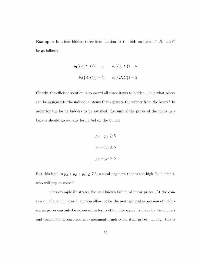
Example: In a four-bidder, three-item auction let the bids on items A, B, and C
be as follows:
b1({A,B,C}) = 6, b2({A,B}) = 5
b3({A,C}) = 5, b4({B,C}) = 5
Clearly, the efficient solution is to award all three items to bidder 1, but what prices
can be assigned to the individual items that separate the winner from the losers? In
order for the losing bidders to be satisfied, the sum of the prices of the items in a
bundle should exceed any losing bid on the bundle:
pA + pB ≥ 5
pA + pC ≥ 5
pB + pC ≥ 5
But this implies pA + pB + pC ≥ 7.5, a total payment that is too high for bidder 1,
who will pay at most 6.
This example illustrates the well known failure of linear prices. At the con-
clusion of a combinatorial auction allowing for the most general expression of prefer-
ences, prices can only be expressed in terms of bundle-payments made by the winners
and cannot be decomposed into meaningful individual item prices. Though this is
52
true at the termination of a combinatorial auction, we argue that linear prices may
still play a role in the early stages of a combinatorial auction, where they may be
used as signals of the value of items if taken individually, before positive synergy is
taken into consideration.
In this chapter, we present a new auction format based on the familiar
assignment problem and show that this is a natural environment for the use of linear
item prices. On one hand, if the bidders do not find the preference restrictions of
the format to be restrictive, we find that this is a compact format which can be used
to find either VCG outcomes (discussed in §3.2) or minimal Walrasian equilibrium
individual item prices (discussed in §3.3). The latter can be implemented in either
a one shot submission of bid tables or through iteratively updated bid tables in a
Dynamic Bid Table Auction, guided at each stage by linear item prices.
If, on the other hand, we are in environment requiring a more robust ex-
pression of preferences (e.g. complements are present), we argue that bid tables
provide a restricted format for which linear prices make sense. In Chapter 4, we
introduce a multi-stage combinatorial auction using a Dynamic Bid Table Auction
as an initial demand revelation phase. Bid tables allow us to utilize the attractive
linear prices as long as it makes sense to do so, until any further bidding requires a
combinatorial element to mitigate positive-synergy exposure. Relative to the SAA,
53

this can be accomplished without negative-synergy exposure, and without the ability
for competitors to signal among themselves.
We begin this chapter with a discussion of the basic properties of bid table
expression.
3.1. Assignment Preferences and the Gross Substitutes Property
Our multi-item auction will have N unique items for sale, with the set of
items denoted I = {1, 2, ...i, ...N}, and the set of M bidders will be referred to as
J = {1, 2, ...j, ...M}. For any bundle or package of items S ⊆ I, each bidder j
perceives some value vj(S) ≥ 0 equal to her utility of receiving this bundle at zero
cost. Further, in this treatment we assume non-negativity (vj(S ∪ {i}) − vj(S) ≥ 0,
∀i, S) and define a bidder’s net utility as uj(S, p) = vj(S) −∑
i∈S pi, where each
component pi of price vector p denotes a price for item i (we assume quasilinear net
utility).
Next, we say a bundle of items S is demanded by j at a price p if S maximizes
net utility for bidder j at p. By denoting the set of all bundles demanded by j at
price p as Dj(p), we may write this mathematically as:
Dj(p) = arg maxS⊆I
uj(S, p)
54

A bidder may demand several bundles at p if each maximizes net utility, and demands
∅ when prices are too high. Additionally, we assume vj(∅) = 0, ∀j.
In a Bid Table Auction, each bidder j has a set of Aj agents he potentially
wishes to satisfy, denoted by the set Kj = {1, 2, ...k, ...Aj}. We assume that each item
in the auction may be consumed by only one agent and that each agent can consume
at most one item. To motivate the proposed use of the Bid Table Auction as the first
stage of a landing slot application, it is useful to think of each agent as representing a
potential flight, and each item as a slot made available to an airline in an airport for
landing a single plane. Often in Chapter 4, the items in the auction will be referred
to as slots, but for the remainder of Chapter 3 we maintain a general attitude with
respect to auction items, believing that there are likely other applications for Bid
Table Auctions.
55

Let vijk denote the utility perceived by bidder j when agent k receives item
i. The preference assumption of the Bid Table Auction can be specified as follows:
vj(S) = max∑
i∈S
∑
k∈Kj
vijk · xijk(AP)
subject to∑
i∈S
xijk ≤ 1, ∀k ∈ Kj
∑
k∈Kj
xijk ≤ 1, ∀i ∈ S
where xijk =
1 if item i is assigned to bidder j’s kth agent
0 otherwise
In short, a bidder’s value for a bundle of items is a maximal value assignment of those
items to her agents. Bidders modeled in this fashion may be said to have assignment
preferences, as their preferences are governed by an assignment network. As is well
known, the constraint matrix of this integer program is total unimodular, indicating
that the problem is solved to integral optimality by its LP relaxation. This implies
that a bidder could rapidly determine her value for any set of items with an LP solver
or faster combinatorial algorithm designed specifically to solve assignment problems,
even for a large value of N.
A bidder with assignment preferences can express his value for every bundle
of items in a bid table containing the values of vijk with a row for each item i and
56
Figure 3.1. Assignment Preferences in a Bid Table
Item aItem bItem cItem d
∣
∣
∣
∣
∣
∣
∣
∣
∣
∣
agent 1 agent 2 agent 30 0 22 5 34 6 40 3 0
∣
∣
∣
∣
∣
∣
∣
∣
∣
∣
column for each agent k. For example, with the bid table of Figure 3.1 we may
determine a bidder’s value for any bundle of items a, b, c, or d if assigned to any
of three possible agents. Considering the values in this bid table, we notice that a
bidder’s value for any single item is simply the maximum value for that row in the
bid table; if a bidder is awarded only one item, the agent that experiences the most
utility from this item will be accommodated. Thus item a by itself is worth 2 units
to the bidder, item b by itself is worth 5 units, item c by itself is worth 6 units,
and item d by itself is worth 3 units. The value for some collection of items is not,
however, necessarily equal to the sum of his values for individual items, as there may
be conflicts when the row maximums occur in the same column. For example, for
bidder j with this bid table vj({b}) = 5, vj({c}) = 6 but vj({b, c}) = 9 6= 5 + 6. We
find vj({a, b, c, d}) = 11 with an optimal assignment of a to the third agent, b to the
second agent and c to the first agent. We notice that to achieve this amount we do
not assign item c to the second agent, despite this being the overall highest value in
the bid table, and also that we choose to assign item a and not item d, despite the
fact that vj({a}) < vj({d}).
57
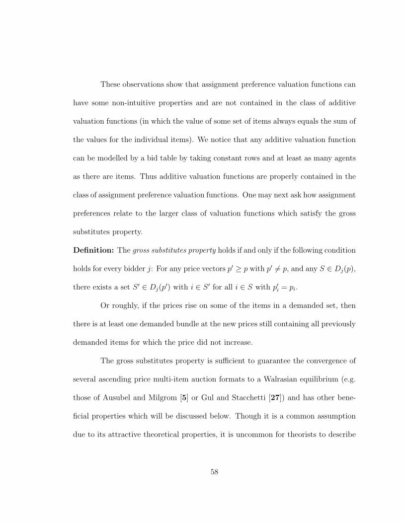
These observations show that assignment preference valuation functions can
have some non-intuitive properties and are not contained in the class of additive
valuation functions (in which the value of some set of items always equals the sum of
the values for the individual items). We notice that any additive valuation function
can be modelled by a bid table by taking constant rows and at least as many agents
as there are items. Thus additive valuation functions are properly contained in the
class of assignment preference valuation functions. One may next ask how assignment
preferences relate to the larger class of valuation functions which satisfy the gross
substitutes property.
Definition: The gross substitutes property holds if and only if the following condition
holds for every bidder j: For any price vectors p′ ≥ p with p′ 6= p, and any S ∈ Dj(p),
there exists a set S ′ ∈ Dj(p′) with i ∈ S ′ for all i ∈ S with p′i = pi.
Or roughly, if the prices rise on some of the items in a demanded set, then
there is at least one demanded bundle at the new prices still containing all previously
demanded items for which the price did not increase.
The gross substitutes property is sufficient to guarantee the convergence of
several ascending price multi-item auction formats to a Walrasian equilibrium (e.g.
those of Ausubel and Milgrom [5] or Gul and Stacchetti [27]) and has other bene-
ficial properties which will be discussed below. Though it is a common assumption
due to its attractive theoretical properties, it is uncommon for theorists to describe
58
applications which give rise to this property, to explain under what conditions it
is a safe assumption to make, or to suggest how to enforce this restriction among
bidders if it is necessary for the convergence of an auction to a desirable outcome.
In this dissertation, we start instead from the assumption of assignment preferences
and show that the gross substitutes property follows as a result.
The following proof of gross substitutes under assignment preferences is con-
structive. Using an LP solver to determine demanded bundles under assignment
preferences may give any demanded bundle after a price increase and will often not
provide the bundle that verifies the validity of the theorem. For any demanded
bundle S∗ before a price increase and a given demanded bundle S ′ after the price
increase, the algorithm described in the proof constructs a new demanded bundle
S∗∗ after the increase, containing all previously demanded items in S∗ for which the
price has not risen.
Theorem 3.1. A valuation function determined by assignment preferences displays
the gross substitutes property.
Proof. Suppose we begin at price vector p1 with a particular demanded bundle
S∗ ∈ Dj(p1) and consider price vector p2 ≥ p1, with p2 6= p1 and a particular de-
manded bundle S ′ ∈ Dj(p2). Under assignment preferences a demanded set is always
supported by an assignment of items to agents which maximizes total value net of
59
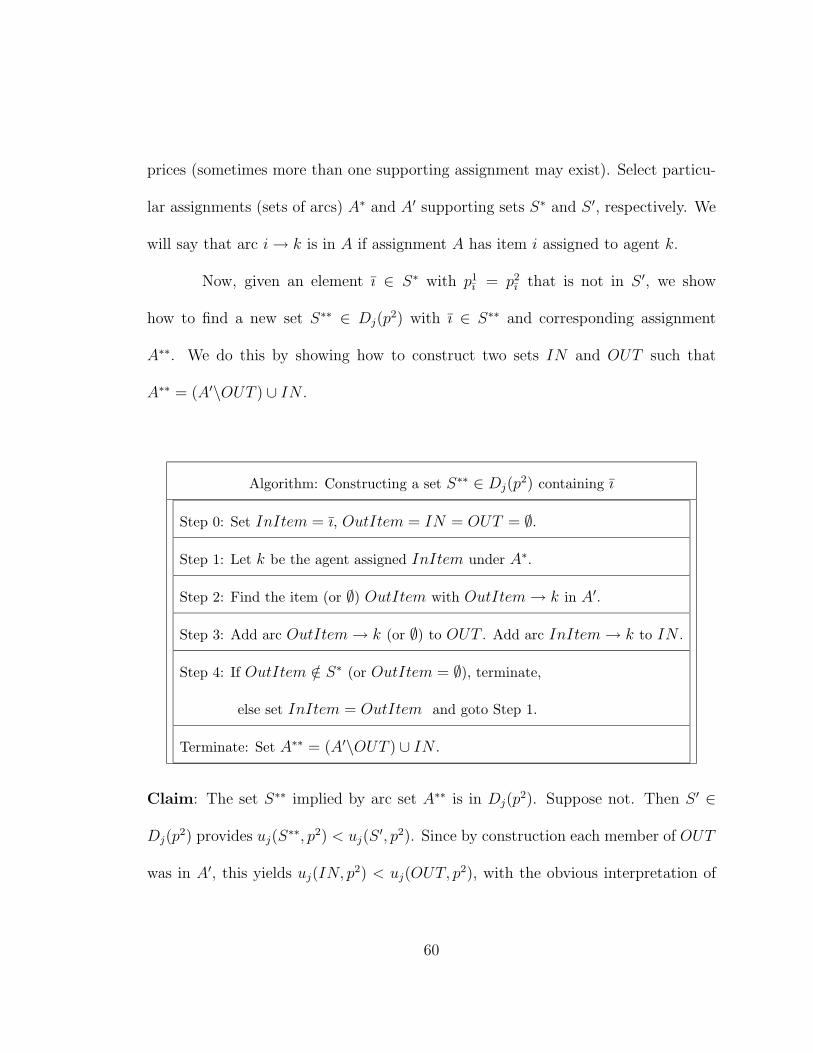
prices (sometimes more than one supporting assignment may exist). Select particu-
lar assignments (sets of arcs) A∗ and A′ supporting sets S∗ and S ′, respectively. We
will say that arc i → k is in A if assignment A has item i assigned to agent k.
Now, given an element ı ∈ S∗ with p1ı = p2
ı that is not in S ′, we show
how to find a new set S∗∗ ∈ Dj(p2) with ı ∈ S∗∗ and corresponding assignment
A∗∗. We do this by showing how to construct two sets IN and OUT such that
A∗∗ = (A′\OUT ) ∪ IN .
Algorithm: Constructing a set S∗∗ ∈ Dj(p2) containing ı
Step 0: Set InItem = ı, OutItem = IN = OUT = ∅.
Step 1: Let k be the agent assigned InItem under A∗.
Step 2: Find the item (or ∅) OutItem with OutItem → k in A′.
Step 3: Add arc OutItem → k (or ∅) to OUT . Add arc InItem → k to IN .
Step 4: If OutItem /∈ S∗ (or OutItem = ∅), terminate,
else set InItem = OutItem and goto Step 1.
Terminate: Set A∗∗ = (A′\OUT ) ∪ IN .
Claim: The set S∗∗ implied by arc set A∗∗ is in Dj(p2). Suppose not. Then S ′ ∈
Dj(p2) provides uj(S
∗∗, p2) < uj(S′, p2). Since by construction each member of OUT
was in A′, this yields uj(IN, p2) < uj(OUT, p2), with the obvious interpretation of
60
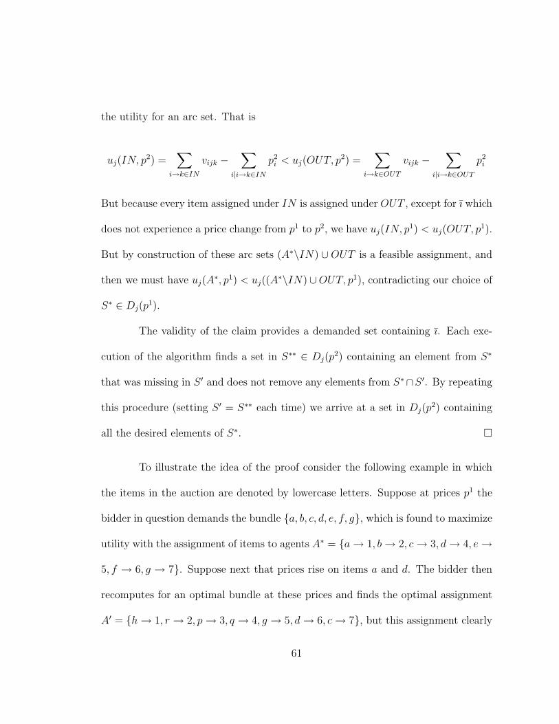
the utility for an arc set. That is
uj(IN, p2) =∑
i→k∈IN
vijk −∑
i|i→k∈IN
p2i < uj(OUT, p2) =
∑
i→k∈OUT
vijk −∑
i|i→k∈OUT
p2i
But because every item assigned under IN is assigned under OUT , except for ı which
does not experience a price change from p1 to p2, we have uj(IN, p1) < uj(OUT, p1).
But by construction of these arc sets (A∗\IN) ∪ OUT is a feasible assignment, and
then we must have uj(A∗, p1) < uj((A
∗\IN)∪OUT, p1), contradicting our choice of
S∗ ∈ Dj(p1).
The validity of the claim provides a demanded set containing ı. Each exe-
cution of the algorithm finds a set in S∗∗ ∈ Dj(p2) containing an element from S∗
that was missing in S ′ and does not remove any elements from S∗∩S ′. By repeating
this procedure (setting S ′ = S∗∗ each time) we arrive at a set in Dj(p2) containing
all the desired elements of S∗. �
To illustrate the idea of the proof consider the following example in which
the items in the auction are denoted by lowercase letters. Suppose at prices p1 the
bidder in question demands the bundle {a, b, c, d, e, f, g}, which is found to maximize
utility with the assignment of items to agents A∗ = {a → 1, b → 2, c → 3, d → 4, e →
5, f → 6, g → 7}. Suppose next that prices rise on items a and d. The bidder then
recomputes for an optimal bundle at these prices and finds the optimal assignment
A′ = {h → 1, r → 2, p → 3, q → 4, g → 5, d → 6, c → 7}, but this assignment clearly
61

does not validate the gross substitutes property; items b, e, and f did not experience
a price increase but they do not appear in the newly demanded bundle.
To apply the algorithm described in the proof, first consider finding a de-
manded set including b. Putting A∗ above A′ and designating destination agents by
column, we see below that agent 2 who was assigned b in A∗ is assigned r in A′:
A∗ : a b c d e f g
↓
A′ : h r p q g d c
− − − − − − − − −
A∗∗ : h b p q g d c
The manipulation performed by the algorithm is in its simplest form here. The value
of A∗∗ at p2 must be at least as much as the value of A′ at p2, or else it would be
possible to switch r in for b in A∗ and receive a higher value at p1, contradicting the
optimality of A∗ as a demanded bundle. This reasoning only holds because the price
of b does not change in the movement from p1 to p2, and because r can be switched
in freely as it is not in A∗.
When we try to find a demanded bundle at p2 containing e, it is not quite
so easy; the agent assigned e under A∗ is assigned g under A′, and since g is already
assigned under A∗ a one-for-one switching argument fails. The algorithm rectifies
62

this by tracing back a path until an item is found that was not allocated under A∗.
For example, the following diagram helps us see that in moving from A∗ to A′ (which
has now been replaced by A∗∗ from the previous step) item e’s agent is reassigned
item g, whose agent in A∗ is reassigned item c, whose agent in A∗ is reassigned by
item p which was unallocated in A∗. The same optimality argument can be used
to show a demanded bundle at p2 including item e; {p → 3, g → 5, c → 7} can be
replaced by {c → 3, e → 5, g → 7} or else the optimality of A∗ is contradicted.
A∗ : a b c d e f g
↓ ↓ ↓
A′ : h b p q g d c
− − − − − − − − −
A∗∗ : h b c q e d g
Similar arguments allow us to settle on a final set A∗∗, containing all items which were
demanded at price p1 for which prices did not increase. The final step is displayed
63
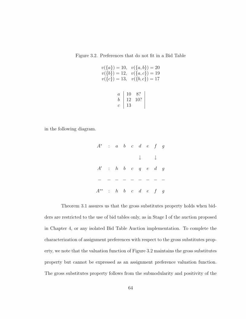
Figure 3.2. Preferences that do not fit in a Bid Table
v({a}) = 10, v({a, b}) = 20v({b}) = 12, v({a, c}) = 19v({c}) = 13, v({b, c}) = 17
abc
∣
∣
∣
∣
∣
∣
10 8?12 10?13
∣
∣
∣
∣
∣
∣
in the following diagram.
A∗ : a b c d e f g
↓ ↓
A′ : h b c q e d g
− − − − − − − − −
A∗∗ : h b c d e f g
Theorem 3.1 assures us that the gross substitutes property holds when bid-
ders are restricted to the use of bid tables only, as in Stage I of the auction proposed
in Chapter 4, or any isolated Bid Table Auction implementation. To complete the
characterization of assignment preferences with respect to the gross substitutes prop-
erty, we note that the valuation function of Figure 3.2 maintains the gross substitutes
property but cannot be expressed as an assignment preference valuation function.
The gross substitutes property follows from the submodularity and positivity of the
64
valuation function. To see that these preferences cannot be expressed as an assign-
ment preference valuation function (or equivalently, as a bid table) notice that the
value of any two items is less than the sum of the values for the individual items,
thus the values for the individual items must all occur in the same column of a bid
table. But now if we attempt to put in a value of 8 into column 2, row a, or a value
of 10 into column 2 row b to express v({a, b}) = 20, we either overvalue the bundle
{a, c} at 21 or the bundle {b, c} at 23. There is therefore no way to express these
gross substitute preferences as assignment preferences.
With Theorem 3.1 and earlier observations we have the following corollary,
where Vadd, VAP , and Vsub denote the classes of valuation functions that have additive
preferences, assignment preferences, and gross substitute preferences, respectively.
Corollary 3.2. Vadd ⊂ VAP ⊂ Vsub
Though all containments in Corollary 3.2 are proper, we note that assignment prefer-
ences do retain some of the interesting properties lost between Vsub and Vadd. Notably,
we can embed in a Bid Table Auction an example from Gul and Stacchetti [27] that
demonstrates the VCG outcome may have lower payments than the lowest Walrasian
Equilibrium. This embedding is shown in Figure 3.3, providing an example of a Bid
Table Auction for which the VCG payments are strictly less than any Walrasian
Equilibrium. In one efficient allocation, bidder X gets {A,D}, bidder Y gets {B}
and bidder Z gets {C}, with VCG payments of 12, 2, and 2, respectively. The lowest
65
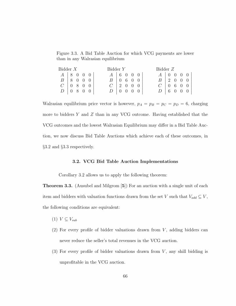
Figure 3.3. A Bid Table Auction for which VCG payments are lowerthan in any Walrasian equilibrium
Bidder XABCD
∣
∣
∣
∣
∣
∣
∣
∣
8 0 0 08 0 0 00 8 0 00 8 0 0
∣
∣
∣
∣
∣
∣
∣
∣
Bidder YABCD
∣
∣
∣
∣
∣
∣
∣
∣
6 0 0 00 6 0 02 0 0 00 0 0 0
∣
∣
∣
∣
∣
∣
∣
∣
Bidder ZABCD
∣
∣
∣
∣
∣
∣
∣
∣
0 0 0 02 0 0 00 6 0 06 0 0 0
∣
∣
∣
∣
∣
∣
∣
∣
Walrasian equilibrium price vector is however, pA = pB = pC = pD = 6, charging
more to bidders Y and Z than in any VCG outcome. Having established that the
VCG outcomes and the lowest Walrasian Equilibrium may differ in a Bid Table Auc-
tion, we now discuss Bid Table Auctions which achieve each of these outcomes, in
§3.2 and §3.3 respectively.
3.2. VCG Bid Table Auction Implementations
Corollary 3.2 allows us to apply the following theorem:
Theorem 3.3. (Ausubel and Milgrom [5]) For an auction with a single unit of each
item and bidders with valuation functions drawn from the set V such that Vadd ⊆ V ,
the following conditions are equivalent:
(1) V ⊆ Vsub
(2) For every profile of bidder valuations drawn from V , adding bidders can
never reduce the seller’s total revenues in the VCG auction.
(3) For every profile of bidder valuations drawn from V , any shill bidding is
unprofitable in the VCG auction.
66

(4) For every profile of bidder valuations drawn from V , any joint deviation by
losing bidders is unprofitable in the VCG auction.
In the sealed-bid Vickrey-Clarke-Groves (VCG) auction ([13], [25], [68])
each bidder submits her true valuation for every possible bundle of items. A winning
allocation is then determined which distributes bundles to bidders so as to maximize
total value. To assure that each bidder has the incentive to reveal her total value
honestly, she pays not her reported value for the bundle she receives, but this value
less an appropriate discount. This VCG discount assures that a bidder does not pay
any more than would be necessary to receive this bundle given her opponents honest
reports, and is equal to the value of the final allocation minus the maximum value
attainable without this bidder. A bidder only decreases her chances of receiving her
efficient allocation of items by misreporting, with no possible gain.
The assurance of honest valuation reporting is well known to be the strength
of the VCG auction, but as Ausubel and Milgrom [5] point out, there are several
drawbacks. Shill bidding occurs when a bidder enters a false identity into the auc-
tion in a way that results in an inefficient allocation or alternative set of payments
which is preferred by the deceitful bidder. Similarly, Ausubel and Milgrom demon-
strate how two or more losing bidders in a VCG auction may increase their bids to
become winning without having to pay for this increase. These problems with the
VCG auction are explored in further depth elsewhere [63], but we note that these
67

difficulties rely on the existence of complementary items, an impossibility when the
gross substitutes condition holds. Theorem 3.3 ensures that these problems of collu-
sive behavior and revenue reduction sometimes recognized as drawbacks to the VCG
auction have no effect when the gross substitutes property holds.
Since the hypotheses for Theorem 3.3 and condition (1) of Theorem 3.3 are
satisfied according to Corollary 3.2, we may conclude that the Bid Table Auction
scenario is one for which the VCG auction attains its full strength. The advantages of
the Bid Table Auction scenario over the general VCG auction context are that each
bidder may simply submit a bid table to express her preferences (a method that is
far more compact than issuing a price for every one of the 2N − 1 possible nonempty
bundles) and the winner determination problem can be solved polynomially using
LP techniques. Both of these features are important for an auction of many items.
Notice that at LaGuardia airport, for example, over 800 slots may be available in a
single day; an auction for these slots which enumerates all possible bundles would
be quite impossible.
In order to run a VCG Bid Table Auction, one must compute both an efficient
allocation and the set of VCG payments for all bidders. To determine an efficient
allocation, the auctioneer, having received bid tables containing the submitted bids
68

of bijk, needs to solve the LP:
zJ = max∑
(i,j,k)∈I×J×Kj
bijk · xijk(P)
subject to∑
i∈I
xijk ≤ 1, ∀(j, k) with j ∈ J and k ∈ Kj
∑
j∈J
∑
k∈Kj
xijk ≤ 1, ∀i ∈ I
xijk ≥ 0, ∀i, j, k
To determine VCG payments, the auctioneer can solve this problem again without
bidder j to find the appropriate discount for bidder j, zJ − zJ\j, where zJ\j denotes
the value of the objective value of P with bidder j removed. The assignment corre-
sponding to zJ determines a bundle Sj with bid value bj(Sj) for each bidder. Each
bidder in the VCG auction receives Sj and pays bj(Sj) − (zJ − zJ\j). For the entire
auction at most M + 1 LPs must be solved. Since there are O(MN2) variables and
O(MN) constraints in each LP, and because it is well known that LPs can be solved
in polynomial time (as a function of the number of constraints and variables), we
conclude that the VCG Bid Table Auction can be solved in polynomial time. There
are in fact combinatorial algorithms for solving assignment problems (of which this
is an instance); see Ahuja, Magnanti and Orlin [1] for a O(M2N3 + MN log MN)
time algorithm.
69

Though Theorem 3.1 allows the application of Theorem 3.3, implying that
because of the gross substitutes property the Bid Table Auction is a good preference
format for a VCG implementation, it also limits the types of possible applications of
the Bid Table Auction to those in which there is no complementarity among items.
In Chapter 4 we discuss an auction for airport landing slots, where bidders (airlines)
perceive the constraints of the Bid Table Auction (inability to use a slot for more
than one flight and inability to land a flight without a slot), but may also perceive
some complementarity among slots (e.g. being able to offer several flights to the
same destination in one day may offer extra profit potential, as discussed above). As
described in Chapter 4, we develop an iterative multi-phase auction, beginning with
a Dynamic Bid Table Auction used to reveal preferences for slots as substitutes, with
complementarity expressed only later in the auction.
3.3. Dynamic Bid Table Auctions
Ignoring for now the issue of complements (i.e. maintaining the assumption
that bidders have assignment preferences), it seems that the primary drawbacks to
the VCG Bid Table Auction are the lack of price discovery and privacy preserva-
tion. Though privacy preservation may in principle be legally enforced, lack of price
discovery may be an inherent concern and discourages the use of a sealed-bid VCG
Bid Table Auction. A bidder may not know how to fill out a bid table with honest
70
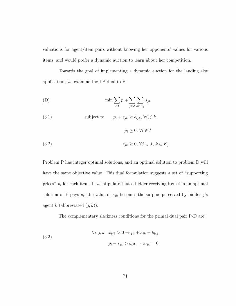
valuations for agent/item pairs without knowing her opponents’ values for various
items, and would prefer a dynamic auction to learn about her competition.
Towards the goal of implementing a dynamic auction for the landing slot
application, we examine the LP dual to P:
min∑
i∈I
pi+∑
j∈J
∑
k∈Kj
sjk(D)
subject to pi + sjk ≥ bijk, ∀i, j, k(3.1)
pi ≥ 0, ∀i ∈ I
sjk ≥ 0, ∀j ∈ J , k ∈ Kj(3.2)
Problem P has integer optimal solutions, and an optimal solution to problem D will
have the same objective value. This dual formulation suggests a set of “supporting
prices” pi for each item. If we stipulate that a bidder receiving item i in an optimal
solution of P pays pi, the value of sjk becomes the surplus perceived by bidder j’s
agent k (abbreviated (j, k)).
The complementary slackness conditions for the primal dual pair P-D are:
(3.3)∀i, j, k xijk > 0 ⇒ pi + sjk = bijk
pi + sjk > bijk ⇒ xijk = 0
71

(3.4)∀j, k
∑
i∈I xijk < 1 ⇒ sjk = 0
sjk > 0 ⇒ ∃i such that xijk = 1
(3.5)∀i ∈ I
∑
j∈J
∑
k∈Kjxijk < 1 ⇒ pi = 0
pi > 0 ⇒∑
j∈J
∑
k∈Kjxijk = 1
Each of these conditions (presented in equivalent pairs) carries an economic inter-
pretation reinforcing the validity of the model. If agent (j, k) is awarded item i,
condition (3.3) implies pi + sjk = bijk, validating our reference to sjk as surplus. If
an agent is not awarded an item in an optimal solution, by condition (3.4) we have
sjk = 0, and then the constraints (3.1) become pi ≥ bijk, ∀i ∈ I; if an agent is
empty-handed at optimality, the optimal dual prices make any item too expensive
for this agent to buy. Similarly, the second statement of (3.4) says that if agent
(j, k) perceives any surplus, then it must be the case that (j, k) received an item.
Further, if we evaluate the potential surplus that item i would bring to agent (j, k)
who receives a different item at optimality, we find sjk ≥ bijk − pi; the price of i is
great enough that a change from the item awarded at optimality to i for agent (j, k)
does not increase surplus. The last pair of conditions, (3.5), state simply that an
item will have a nonzero price only if it is received by some agent.
72
Definition: An allocation of bundles to bidders (S1, S2, ...Sj...SM) and price vector
p constitute a Walrasian equilibrium if and only if for every bidder j, Sj ∈ Dj(p).
Theorem 3.4. Assuming truthful demand reporting and assignment preferences,
the allocation (S1, S2, ...Sj...SM) given by an optimal solution to P together with
prices for items p = (p1, p2, ...pi...pN) given by the corresponding dual solution to D
constitutes a Walrasian equilibrium.
Proof. Suppose not: there is some bidder j and some bundle Sj with j strictly
preferring Sj to Sj. Equivalently,
bj(Sj) −∑
i∈Sj
pi > bj(Sj) −∑
i∈Sj
pi
where bj(Sj) and bj(Sj) are supported by agent sets K and K, respectively. Com-
plementary slackness conditions (3.3) provide bijk − pi = sjk for each item i assigned
to j in Sj, yielding bj(Sj) −∑
i∈Sjpi =
∑
k∈K sjk. Similarly, constraints (3.1) yield
∑
k∈K sjk ≥ bj(Sj) −∑
i∈Sjpi. Together this implies
∑
k∈K
sjk >∑
k∈K
sjk
but with sjk = 0 in the optimal solution of D for any agent k /∈ K, and sjk ≥ 0 for
all tasks, we have
∑
k∈K∩K
sjk >∑
k∈K
sjk
73

a contradiction. �
Among all dual solutions there exists one solution that is bidder-optimal, the
lowest Walrasian equilibrium. The existence of a Walrasian equilibrium under the
gross substitutes property is established by Kelso and Crawford [33]. The uniqueness
of this bidder-optimal Walrasian equilibrium when the gross substitutes property
holds follows naturally from the work of Gul and Stacchetti [26], who demonstrate
the lattice structure of Walrasian Equilibria under gross substitutes. In our case,
this existence and uniqueness is guaranteed because the gross substitutes property
holds by Theorem 3.1. It is known from the work of Demange, Gale, and Sotomayor
[19] that versions of the “Hungarian algorithm” (a primal/dual method for solving
assignment problems) yield this lowest Walrasian equilibrium in the special case that
Aj = 1, ∀j.
As in Demange, Gale, and Sotomayor [19], the Hungarian algorithm finds an
efficient allocation in a Bid Table Auction and the prices used in its solution provide
an optimal solution to the dual problem D, together forming a Walrasian equilibrium,
from Theorem 3.4. In general, however, this method produces Walrasian prices that
are greater than or equal to the actual lowest Walrasian equilibrium prices for a
Bid Table Auction. This is because according to formulation D alone, the price a
bidder pays may be determined by one of her own agents, as if own agents must
price-compete among themselves.
74
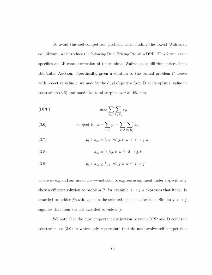
To avoid this self-competition problem when finding the lowest Walrasian
equilibrium, we introduce the following Dual Pricing Problem DPP. This formulation
specifies an LP-characterization of the minimal Walrasian equilibrium prices for a
Bid Table Auction. Specifically, given a solution to the primal problem P above
with objective value z, we may fix the dual objective from D at its optimal value in
constraints (3.6) and maximize total surplus over all bidders.
max∑
j∈J
∑
k∈Kj
sjk(DPP)
subject to z =∑
i∈I
pi +∑
j∈J
∑
k∈Kj
sjk(3.6)
pi + sjk = bijk, ∀i, j, k with i → j, k(3.7)
sjk = 0, ∀j, k with ∅ → j, k(3.8)
pi + sjk ≥ bijk, ∀i, j, k with i 9 j(3.9)
where we expand our use of the →-notation to express assignment under a specifically
chosen efficient solution to problem P; for example, i → j, k expresses that item i is
awarded to bidder j’s kth agent in the selected efficient allocation. Similarly, i 9 j
signifies that item i is not awarded to bidder j.
We note that the most important distinction between DPP and D comes in
constraint set (3.9) in which only constraints that do not involve self-competition
75

are enforced. That is, form the set of constraints (3.9) from constraint set (3.1) of
formulation D by removing all constraints pi + sjk ≥ bijk involving both an item i
and its winner, bidder j. This approach is equivalent to re-solving the primal allo-
cation problem P and the dual problem D with a Hungarian primal/dual method
after lowering all non-winning entries in a winning row of a bid table to zero. We
use the formulation DPP in the following proof as it provides an interesting interpre-
tation as a price adjustment procedure; starting with an efficient allocation and the
optimal solution of D, lower the prices on winning bidders as long as no one com-
plains, any violated constraint from (3.9) interpreted as a possible complaint from
another bidder. Knowing that prices may be easily and transparently adjusted to
a unique minimal Walrasian equilibrium is a primary benefit of Theorem 3.1 (gross
substitutes). We will use this unique price vector in a multi-round setting, using Bid
Table Auctions as a mechanism of demand revelation with distinct meaningful price
signals at each round of submission. We now prove that we achieve these desirable
price signals formally.
Theorem 3.5. Given an optimal solution to the primal problem P with objective
z, solving DPP to maximize bidder surplus yields the lowest Walrasian equilibrium
price vector p∗.
Proof. Begin with price vector p1 which is an optimal solution to D and therefore
a Walrasian equilibrium price by Theorem 3.4. Note that this optimal solution to
76
D gives a feasible solution to DPP with constraints (3.7) and (3.8) holding by the
strong duality of P and D. Lowering any component p1i and raising the corresponding
component s1jk by the same amount (where i is assigned to j, k in the solution to P)
will have no effect on constraints (3.6), (3.7) or (3.8).
Claim: If such a shift from price to surplus does not violate constraints (3.9) the
resulting price vector continues to support a Walrasian equilibrium. If not, some
other bidder j’s agent j, k not assigned item i would prefer item i to whatever item
that has been assigned to j, k (if any). This implies that bijk − pi > sjk which would
violate the corresponding constraint from (3.9).
We therefore proceed to shift price to surplus until any possible shift causes
a violation of some constraint from (3.9), achieving a price vector p2.
Claim: p2 is the lowest Walrasian equilibrium price vector. Suppose not: let p3 6= p2
be the lowest Walrasian price vector. From the lattice theory of Walrasian equilibria
when the gross substitutes condition holds (as established by Gul and Stacchetti
[26]) this Walrasian Equilibrium price is unique, and for every component p3i ≤ p2
i .
Since p3 6= p2 there must be some i for which p3i < p2
i . Since our price-to-surplus
shifting procedure has terminated, a shift from p2i to p3
i must violate some constraint
from (3.9), thus we have the following inequality holding for some j, k with i not
assigned to bidder j:
p3i + sjk < bijk
77

But now at price vector p3, bidder j who is allocated bundle Sj + {i} prefers
bundle Sj ∪ {i} to Sj, implying that p3 does not support a Walrasian equilibrium, a
contradiction. �
Now that we have shown how the lowest Walrasian price vector will be
computed at each round, we propose the Dynamic Bid Table Auction proceeding
in multiple rounds as follows. Accept bid tables from all bidders and determine a
winning allocation (solution to P) using any technique (e.g. the Hungarian algo-
rithm). Adjust the prices as suggested in Theorem 3.5 to find an optimal solution to
DPP, and therefore the set of unique lowest Walrasian equilibrium prices. Announce
winning prices and allow bidders to adjust their bid tables subject to the following
rules:
• Any bid in a non-winning row of a bid table must be raised at least to the
current price for that item (row) plus one price increment, or else it may
not be altered for the remainder of the auction.
• A bidder who does not wish to increase an entry to the required amount
may increase it to a price below the current price plus one increment. This
is the bidder’s “last-and-best” offer.
The auction then continues by computing a new set of winning bids and prices, and
the process repeats until no one wishes to raise any bid table entries any further.
78
To show that this procedure progresses to a desirable equilibrium, assume
that each bidder perceives a set of maximum bid table values, vijk. We would expect
to see these entries from honest bidders in the direct revelation VCG as in §3.2,
and now show that the dynamic game converges to the same outcome as the direct
revelation game, given some assumption of straightforward bidding. In this Dynamic
Bid Table Auction scenario, we will say that a bidder bids straightforwardly if she
increases a bid table bijk in a non-winning row by the minimal increment whenever
the potential surplus vijk−pi for agent (j, k) is greater than the actual current surplus
for agent (j, k), sjk = vıjk − pı, where ı is the item currently awarded to agent (j, k).
Here the modifier actual and ‘bar’ over the s emphasize that this is the actual surplus
as perceived by the bidder, not the apparent surplus which may be computed using
her revealed information: sjk = bıjk − pı. In either case, this surplus will be zero if
no item is awarded to agent k. We also assume that if a straightforward bidder is
asked to raise a bid table value above vijk, then she will raise it to vijk, reporting her
true valuation as she loses eligibility to alter the entry further.
Theorem 3.6. A Dynamic Bid Table Auction with straightforward bidders termi-
nates at an efficient equilibrium of the direct revelation Bid Table Auction, with the
unique lowest Walrasian equilibrium prices.
Proof. Part A: First, we show that the allocation at termination is an efficient
outcome of the direct revelation game. Suppose not. Let A be the allocation at
79
termination of the dynamic auction with current bid table values bijk. By supposition
there is an allocation A such that
(3.10)∑
A
xijk · vijk >∑
A
xijk · vijk
where the summation over an allocation signifies summation over all i, j, k with
values of xijk given by that allocation. Because we have assumed that bidders bid
straightforwardly and that the dynamic auction has terminated, for any bid table
column j, k which is allocated item i under allocation A and ı under A, it must be
the case that vıjk − pı ≤ vijk − pi (if not the straightforward bidder would want to
continue bidding on ı). This inequality also holds (reflexively) for any agent j, k that
is awarded the same item under both allocation A and A. For any j, k allocated
item ı under A which is not allocated an item under A, this condition becomes
vıjk − pı ≤ 0. Finally, by individual rationality we also have that 0 ≤ vijk − pi for
any i allocated to j, k under A (particularly we take this inequality for any columns
j, k which are for agents receiving items in both allocations, allocated items under
A but not under A). We then sum these three sets of inequalities, selecting (and
multiplying by xijk) the appropriate one for each agent j, k who receives items in
80
either allocation A or A, or both, yielding:
∑
A
xijk · (vijk − pi) ≤∑
A
xijk · (vijk − pi)
∑
A
xijk · vijk ≤∑
A
xijk · vijk(3.11)
with the second inequality following since each item is allocated exactly once in
each allocation, allowing us to cancel the sum of all pis from each side. But (3.11)
contradicts (3.10), with the desired result following.
Part B: Next we show that the prices at termination of the dynamic schedule
auction are the lowest Walrasian equilibrium prices for the direct revelation schedule
auction. Using Theorem 3.5, this is equivalent to showing that the solution to the
pricing problem DPP using the value z (computed using values from vijk) has equal
values for all pi to the solution of DPP using value z (computed using bijk).
Given that the optimal allocation is unchanged by increasing all bijk values
to their reservation point vijk from Part A, increase all bijk values to vijk and si-
multaneously increase every surplus sjk by the same amount wherever i is allocated
to j, k. We claim that this provides a solution to DPP using value z with identi-
cal values of all pi, as desired. Clearly, the simultaneous shift of sjk values with
bijk values upholds DPP constraints (3.6) and (3.7). Constraints (3.8) are upheld
since sjk only changes for columns which win items, while a violation of a constraint
81

from (3.9) would imply a violation of a termination condition. Since none of the
constraints of DPP are violated, our new solution must be feasible to DPP. Since
any increase of the DPP objective function must be accompanied by an equivalent
increase to the primal objective z, and because we have achieved all such increase as
surplus, we may be assured that our new objective function is optimal. Since no pi
values have changed we have the same lowest Walrasian equilibrium price vector at
the termination of the Dynamic Bid Table Auction and in the direct revelation Bid
Table Auction, as desired. �
Part B of this proof demonstrates the desirable privacy-preservation property
of the Dynamic Bid Table Auction relative to the static revelation version: the actual
surplus each bidder perceives need not be revealed in the dynamic case, only that
surplus is at least one increment. By making the bid increment smaller we may in
this way approach maximal privacy-preservation.
The results of this section hold under the assumption that each bidder’s
preferences are modeled accurately in bid tables, an assumption which we have shown
to be more restrictive than the gross substitutes property. Recent trends in auction
design suggest that the use of auctions which work well under the gross substitutes
property (e.g. those of Gul and Stacchetti [27] or Ausubel [2]) may be used to reveal
information necessary for bidders to make decisions in an auction allowing for more
general expression of preferences, those for which gross substitutes does not hold. At
82
the end of a Dynamic Bid Table Auction, each bidder should be comfortable that he
has bid enough on individual items (time-slots in the airport scenario) without being
exposed to the risk of paying too much for substitute items. When this Dynamic
Bid Table Auction is used as the first stage in the multi-stage auction described in
Chapter 4, the bidders should not have exposed themselves to the risk of paying too
much for an item or set of items in an attempt to secure a package of complements,
being assured of participation in later stages which allow for expression of positive
synergy.
83

CHAPTER 4
A Three-Stage Auction for Airport Landing Slots
It has been suggested recently that a multi-item auction may more efficiently
allocate airport landing slots at certain high-density airports, some of which are
already slot-controlled (LaGuardia, Washington National, Kennedy International,
and O’Hare International). Currently, administrative practices and “grandfathering”
procedures are used to determine which airlines have the right to land at these
airports, though these measures have led to apparent inefficiencies, such as the “baby-
sitting” of slots with small inefficient flights in order to maintain landing rights under
the FAA’s “use-it-or-lose-it” policy [6]. Since a similar rejection of the inefficiency
and potential inequity of an administrative allocation caused the FCC’s adoption of
the SAA, it seems natural to consider a similar change for the FAA’s allocation of
controlled landing slots.
In this chapter we lay the groundwork for a new three-stage auction design
suited to the landing slot application. We demonstrate several of its features and
explore how it may be tailored to fit this application specifically. Though the general
version of this auction may be of interest for use in other applications, we first explore
the features of the landing slot scenario to motivate the structure of the model in
84
§4.1. §4.2 gives an overview of the entire three-stage auction process, with §4.3 and
§4.4 providing details for Stages II and III, respectively.
4.1. Auctioning Landing Slots
An extensive examination of the problem of allocating scarce landing slot
rights is given by the consulting firm DotEcon [21] who argue strongly in favor
of a market based allocation mechanism over an administrative procedure. Ball,
Donohue, and Hoffman [6] provide a similar investigation of the situation in the U.S.,
with a focus on safety considerations and suggestions for auction design. Rather than
reiterate these arguments to motivate the potential benefits of a landing slot auction,
we refer the interested reader to these sources for motivation of the problem, and
only briefly explore the auction design problem based on several features advocated
in that literature.
We first note that there is reason to believe that the demand for the rights
to take-off or land an aircraft at a given airport may be adequately controlled by
the regulation of only one of these movements. Since an aircraft cannot depart
from an airport without first arriving, the volume of departures will be regulated
implicitly when the right to land is properly regulated. Further, in-air delays are
more expensive than ground delays; thus it makes sense that landing rights should
be the more clearly defined and tightly controlled of the two movements.
85
For safety reasons the exact departure and landing times must be left in the
hands of air-traffic control, though the volume of possible air movements in a given
interval or block of time may be controlled without specifying an exact time. The
items for sale in the auction will therefore be rights to land in a particular short
interval (say 15 minutes) at a particular slot-controlled airport. Owners of such
rights will be held responsible for landing within this period and may be penalized
for gross or regular non-adherence to this schedule. In case of poor weather this time
period may be altered by means of ground delay under the authority of air-traffic
control.
As suggested by Ball, Donohue, and Hoffman [6], it will be beneficial to have
at least two, and potentially three markets for landing slot rights: a long-term market
where airlines purchase rights to land at a particular airport, held well in advance
of actualization; a secondary market held when demand and scheduling becomes
known, a month or so in advance of actualization, allowing airlines to buy or sell
slots from one another as needed; and a third market for day-of-operations exchanges
when weather and cancellation information is known. In this chapter we focus on
the first market, in which airlines buy long term leases to land during a particular
time of day, on a particular day of the week, in a particular season, repeatedly for
5 to 10 years. In this market, airlines establish their long term operational strategy
86

and stake their claim to provide a particular service or control a certain share of the
consumer market.
In this chapter we suggest a new combinatorial auction design for this long-
term market. Few, if any, available auction designs are capable of handling the
very large number of slots that would be up for sale at a single airport. At least
eight hundred time slots are utilized in a day at LaGuardia according to the Official
Airline Guide (OAG), while the FCC has been skittish about auctioning more than
a dozen spectrum licenses in a combinatorial format. The seminal work of Rassenti,
Smith and Bulfin [59] suggests a network wide auction of links between airports, but
their simulations endorsing the use of a combinatorial format make use of only six
items at auction. Because there are only a handful of airports currently under slot
restrictions, we feel justified in restricting ourselves to an auction at a single airport
where the number of items at auction may be several hundred, rather than deal with
the possibility of around a hundred thousand in a full network auction. Also, at
the recent NEXTOR workshop [49] devoted to the use of market mechanisms for
congestion management in aviation, there seemed to be a general consensus that
market mechanisms should be introduced one congested airport at a time.
As noted above, the desire for combinatorial auctions results from “synergy”
in the preference structure of a bidder, which may be positive when the bundle
contains mostly complements, or negative if the bundle contains mostly substitutes.
87
What kind of synergy would we expect to find in a long-term airport landing-slot
auction? We argue that there are natural reasons for expecting airlines to find
landing slots as both substitutes and complements, adding a level of complexity that
must be reflected in the auction design.
Examination of airport scheduling information in the OAG reveals two po-
tential forms of complementarity among bundles of slots which stem from the basic
operational strategies of the airlines. The first is that of “banking” in which airlines
schedule several planes to land around the same time (usually at a hub location)
in order to collect the passengers together and regroup them on connecting flights.
This will add value to certain bundles of closely grouped slots (positive synergy in
the eyes of bidders with this strategy).
We also recognize a second apparent complementarity among bundles of slots
which may be referred to as “shuttling”. Airlines gain efficiency and market power
by providing a shuttle service between major airports. Airlines with this operational
strategy in mind will value bundles with regularly spaced time slots more than the
sum of the individual slots, another source of positive synergy.
Negative synergy in the proposed market for landing slots comes from the
logistical constraint that a flight may only use one time slot. If an airline is only
interested in a single flight at the airport in question, for example, then the value of
a bundle of more than one time slot is the value of the most valued individual slot.
88

This negative synergy due to conflict may persist when a larger number of flights is
considered. Suppose airline j has two potential flights to be considered, high profit
flight-1 which is valued at 10 regardless of which of slots A or B it lands in, and
a lower profit flight-2 which is valued at 7 in either slot A or B. We then have
vj({A}) = vj({B}) = 10 (since either one on its own can accommodate flight-1),
but vj({A,B}) = 17 < vj({A}) + vj({B}), confirming the negative synergy. This
example elucidates a general phenomenon of negative synergy due to the underlying
assignment constraints that each airline must face. In order to protect a bidder from
negative-synergy exposure, our multi-stage auction begins with a price-vector agent
format (i.e. bid tables) and continues to respect that structure for the duration of
the auction.
The interplay between the Dynamic Bid Table Auction, itself a price-vector
agent implementation, and the other stages of the auction are outlined in the fol-
lowing section that introduces the basic framework of the auction mechanism we
propose for airport landing-slot auctions, called a Schedule Auction.
4.2. Schedule Auction Framework
The mechanism we propose proceeds in three stages, as shown in Figure
4.1. The first two stages are designed to reveal price information while mitigating
the exposure problem, a phenomenon recognized as a primary reason for the use of
combinatorial auctions. If items are awarded singly an honest bidder revealing price
89
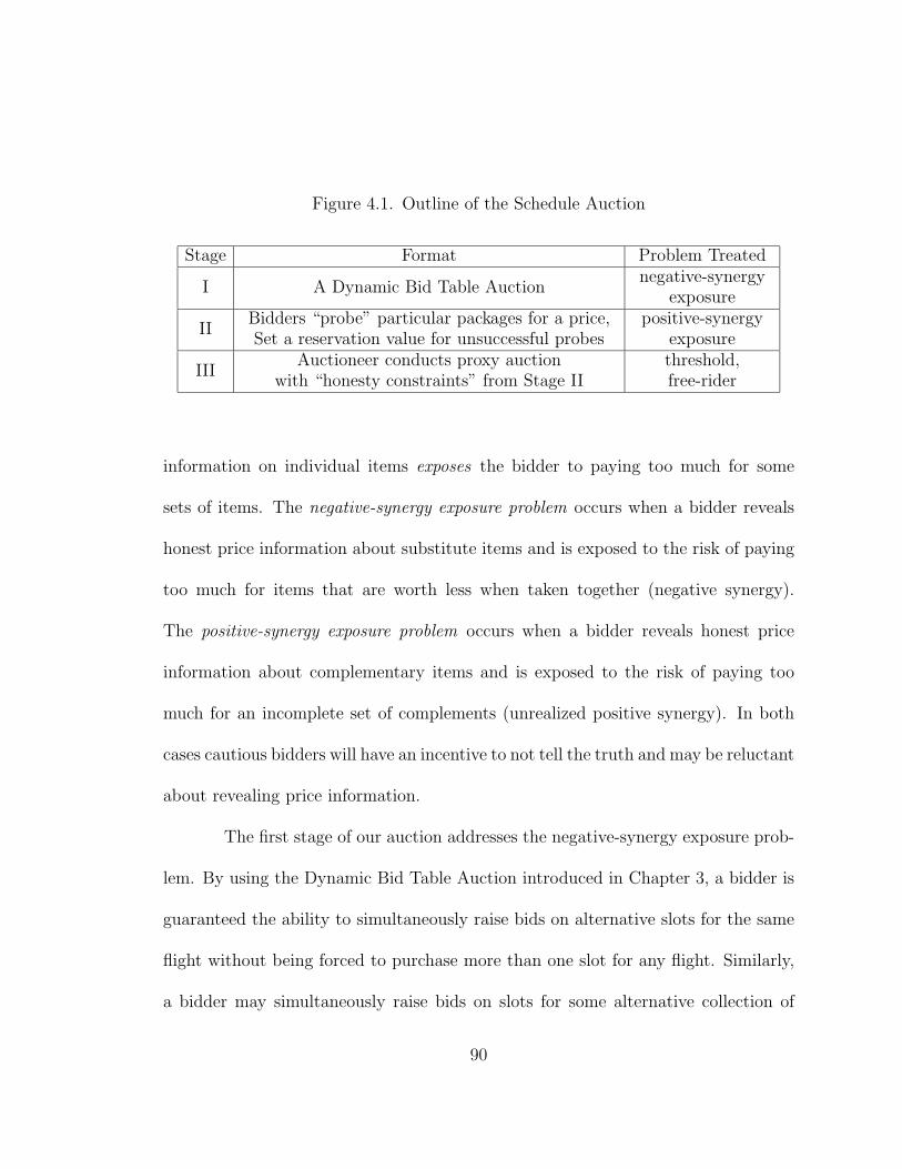
Figure 4.1. Outline of the Schedule Auction
Stage Format Problem Treated
I A Dynamic Bid Table Auctionnegative-synergy
exposure
IIBidders “probe” particular packages for a price,Set a reservation value for unsuccessful probes
positive-synergyexposure
IIIAuctioneer conducts proxy auction
with “honesty constraints” from Stage IIthreshold,free-rider
information on individual items exposes the bidder to paying too much for some
sets of items. The negative-synergy exposure problem occurs when a bidder reveals
honest price information about substitute items and is exposed to the risk of paying
too much for items that are worth less when taken together (negative synergy).
The positive-synergy exposure problem occurs when a bidder reveals honest price
information about complementary items and is exposed to the risk of paying too
much for an incomplete set of complements (unrealized positive synergy). In both
cases cautious bidders will have an incentive to not tell the truth and may be reluctant
about revealing price information.
The first stage of our auction addresses the negative-synergy exposure prob-
lem. By using the Dynamic Bid Table Auction introduced in Chapter 3, a bidder is
guaranteed the ability to simultaneously raise bids on alternative slots for the same
flight without being forced to purchase more than one slot for any flight. Similarly,
a bidder may simultaneously raise bids on slots for some alternative collection of
90
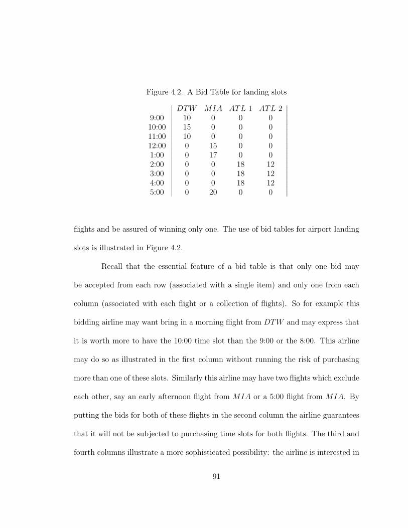
Figure 4.2. A Bid Table for landing slots
9:0010:0011:0012:001:002:003:004:005:00
∣
∣
∣
∣
∣
∣
∣
∣
∣
∣
∣
∣
∣
∣
∣
∣
∣
∣
∣
DTW MIA ATL 1 ATL 210 0 0 015 0 0 010 0 0 00 15 0 00 17 0 00 0 18 120 0 18 120 0 18 120 20 0 0
∣
∣
∣
∣
∣
∣
∣
∣
∣
∣
∣
∣
∣
∣
∣
∣
∣
∣
∣
flights and be assured of winning only one. The use of bid tables for airport landing
slots is illustrated in Figure 4.2.
Recall that the essential feature of a bid table is that only one bid may
be accepted from each row (associated with a single item) and only one from each
column (associated with each flight or a collection of flights). So for example this
bidding airline may want bring in a morning flight from DTW and may express that
it is worth more to have the 10:00 time slot than the 9:00 or the 8:00. This airline
may do so as illustrated in the first column without running the risk of purchasing
more than one of these slots. Similarly this airline may have two flights which exclude
each other, say an early afternoon flight from MIA or a 5:00 flight from MIA. By
putting the bids for both of these flights in the second column the airline guarantees
that it will not be subjected to purchasing time slots for both flights. The third and
fourth columns illustrate a more sophisticated possibility: the airline is interested in
91

running two mid-afternoon flights from ATL, but wants to pay less for the second
one. By bidding as indicated in Figure 4.2, the airline will pay at most 18 for the
first of the mid-afternoon slots and 12 for the second afternoon slot it receives.
Stage I of the auction proceeds by bidders submitting and adjusting bid
tables like the one in Figure 4.2. Following the submission of bid tables by all
bidders the auctioneer announces a current winning allocation and a price for each
item. These prices will be dual prices from the primal allocation problem which are
equal to the lowest Walrasian equilibrium prices (as shown in §3.3). Bidders then
adjust and resubmit their bid table entries according to the following eligibility rules:
• an entry may not decrease
• an entry in a non-winning bid table row must be raised to at least the current
price for that row plus one increment, or else a “last and best” entry may
be made that cannot be adjusted again for the remainder of the auction
• entries in a winning row of a bid table need not be adjusted.
Such rules are necessary for this stage to ensure that the auction proceeds at a
healthy pace and so that bidders may not lay in waiting without revealing their
intentions.
When a round occurs in which no bidder chooses to increase any bid table
entry, the auction enters Stage II, designed to mitigate the positive-synergy exposure
problem by accepting all-or-nothing package bids. In this stage each bidder is asked
92
in turn to submit a package of items and a price which guarantees to increase auction
efficiency if accepted. If this bid survives the remainder of the auction, the bidder
receives the items in the package, paying no more than the specified price, as well as
any items she may still be winning individually from Stage I at the prices determined
there. Because a particular package may be intended for a specific collection of flights,
a bidder is allowed to specify the bid-table columns (agents) associated with these
flights so that the auctioneer may remove them from her bid table. This will ensure
that multiple slots are not won for the same flight, one from the bid-table and one
from the package bid.
Using the techniques described in §4.3, each bidder in Stage II can “probe”
the market to determine what price must be offered for a particular bundle of items.
Once he has found a subset for which he is willing to pay the necessary amount,
he may submit this package/price pair which is guaranteed to be winning, until
(possibly) it is “knocked out” by another bidder’s package bid. We suggest that
probing may proceed in a round-robin fashion, where the order of bidding is generated
randomly for each round. Further, if the results of Stage I (i.e. the final bid tables)
and each of the provisionally winning Stage II bids are released to the bidders, they
may continue to probe while waiting their turn. This will allow bidders to explore
more scenarios and potential business plans, so that many package bids may be
evaluated in preparation for a turn to bid. If instead bidder privacy is deemed more
93
valuable in a particular application, the provisionally winning Stage II bids and final
Stage I bids maybe known only to the auctioneer, but then more time should be
given to each bidder for probing, since this would be the bidders’ only way to learn
about the competition.
An important feature of our model is the order in which different types of
preference information is revealed over the course of the auction, postponing the
solution of difficult computational problems until they are assured to be necessary.
For example, the all-or-nothing package bids of Stage II introduce a high level of
computational difficulty (we discuss the NP-completeness of the feasibility problem
with such bids in §4.3). By first executing a Dynamic Bid Table Auction in Stage
I, we eliminate from consideration any package bid which doesn’t at least beat the
“individual prices” for the items in the package. We place Stage I before Stage
II in order to drive up these prices on individual items as much as possible before
considering any package bids, eliminating as many as possible from consideration
since they are more difficult to handle. We then shift the computational burden to
the bidder who must decide which bundle to bid on in Stage II.
This idea of first driving up individual prices and then shifting computational
burden to the bidders is present in the PAUSE auction of Kelly and Steinberg [32].
However, the use of SAA in their own Stage 1 does not address the negative-synergy
exposure problem, unlike the Bid Table Auction. Indeed, we expect that if a Dynamic
94

Bid Table Auction were simply used to replace the SAA in Stage 1 of Kelly and
Steinberg’s model, bidders would experience less negative-synergy exposure and be
able to bid more aggressively on individual items. The resulting higher prices on
individual items will in turn ease more of the computational burden of package
bidding.
We note that the recent hybrid auction design of Ausubel, Cramton, and Mil-
grom [4] provides similar advantages over the adaptive user selection mechanisms,
through separation of the auction into demand revelation and sealed-bid phases. We
note, however, that our design provides an alternative to their method, with a de-
mand revelation stage for complementary packages (Stage II), and explicit reduction
of negative-synergy exposure through a price-vector agent format.
In Stage I of the Schedule Auction, we believe that new market entrants will
have a greater opportunity to make simultaneous aggressive bids relative to the SAA,
forcing incumbents to either let them into the market or share the burden of keeping
them out. Fair entry into the market place has been an expressed consideration in
the airport landing slot context, and we feel that the use of the Dynamic Bid Ta-
ble Auction will also enhance the ability of new entrants to compete in the market
by decreasing the opportunity for the “bullying” punishment strategies described
by Cramton and Schwartz [15] for the SAA. In this behavior observed in actual
SAA implementations, an aggressive bidder drives up the price on a competitor as
95
punishment for placing a competing bid. In the Dynamic Bid Table Auction this
aggressive behavior is not possible; only price signals are revealed to the bidder at
each iteration, making it hard to tell who to bully. Further, each bidder simultane-
ously competes on several substitutable items without exposure to receiving more
than needed; a bullying bidder would have to drive up the price on all items for the
punishment strategy to be effective, increasing his chances of winning an item that
was bid only to punish a competitor.
Another potential improvement on the approach of available combinatorial
auction methods involves the threshold problem. The threshold problem is the po-
tential inability of an individual bidder to displace an inefficient package bid without
the coordinated efforts of other bidders. Take for example a three bidder auction
with four items A, B, C, and D. Suppose that v1({A,B}) = v2({C,D}) = 6,
v3({A,B,C,D}) = 9, and for all other bundles and bidders vj(S) = 2 |S|. The
threshold problem occurs if a bid of 9 on all four items is made by bidder 3 and
accepted: neither of the other two bidders is able to submit a package bid on their
own that will knock out this bid, but if they were to bid 5 each on {A,B} and
{C,D}, respectively, they can clearly overcome the bid of 9 and achieve a more
efficient solution.
There is, however, a disincentive to honest revelation in these circumstances
known as the free-rider problem. If bidder 1 suspects or knows that v2({C,D}) = 6,
96
he may try to only bid 4 on {A,B} hoping that bidder 2 will shoulder more of the
burden necessary to overcome bidder 3. If bidder 2 takes the same approach, bidding
only 4 hoping that bidder 1 will bid 6, the two may fail to overcome the bid of 9 by
only bidding a combined 8.
To combat the threshold problem Banks, Ledyard and Porter [7] and Kelly
and Steinberg [32] suggest the use of a publicly available stand-by queue containing
voluntarily submitted package/price bids that a bidders may select to combine with
their own bids to make winning package bids. Though this technique does address
the threshold problem, it is fully open to the difficulties of the free-rider problem. We
instead suggest the use of a third auction stage to combat both of these problems.
Rather than consider collections of non-winning package bids in our own Stage II, our
auction format does not address the threshold problem until Stage III. The reasoning
for doing this is similar to the reasoning for the separation of Stage I and Stage II:
We do not begin to admit package bids in Stage II until after we know such bids
will beat the individual item prices derived in Stage I; similarly, we do not want to
consider a collection of individual package bids displacing some other collection of
package bids until no more improving individual package bids are possible.
In order to combat the threshold problem and the free-rider problem simul-
taneously, we conduct a sealed-bid auction in Stage III which takes bid information
from Stage I and II and attempts to improve upon the allocation found at the end of
97
Stage II. When a bidder probes a particular set in Stage II, she is told a price that
she must pay in order to become the winner of this bundle, at least provisionally. If
she chooses to accept the reported price at the time of probing, she becomes the pro-
visional winner of this package. If she decides instead that her value for this bundle
is lower than the minimum necessary to become winning unilaterally, she must wait
until Stage III to submit her bid on this bundle, hoping that it may then become
part of the winning collection of bids.
In order to assure participation in Stage II, a bid on a particular bundle
in Stage III must be less than would become winning in Stage II. If a bidder (dis-
honestly) passes on the price of a bundle in Stage II, he forfeits his right to bid
this amount in Stage III. Further, every Stage III bundle bid is screened to ensure
that it would not have been winning in Stage II; thus an unprobed bid is treated
just as a rejected probed bid. For an honest bidder, this rule will not be restrictive
when the current (probe) price for a bundle is higher than his true valuation for that
bundle. We therefore refer to these restrictions as honesty constraints. If a bundle
bid is winning at the termination of Stage II, however, the auction has not neces-
sarily discovered the value of the bundle to the bidder. It therefore puts no honesty
constraint on a Stage III bundle bid for a bidder that is winning that bundle at the
end of Stage II. This provides an additional incentive for participation in Stage II;
a bundle won in Stage II may be protected by an arbitrarily large bid in Stage III,
98

despite limitations on the bids of competitors. Within Stage III, the auctioneer will
determine an allocation that is more efficient than the one achieved in Stage II (if
possible), and compute competitive prices as described in §4.4 and in Chapter 5.
Strategically, this design should make free-riding as difficult as possible.
When a bidder decides not to place any further bids on any bundles in Stage II
(i.e., when a bidder passes on the opportunity to bid when it is her turn), she relin-
quishes the ability to bid any amount above the probe price in the final sealed-bid
round for any bundle she is not winning at the end of Stage II. This makes it unwise
not to accept the probe price except when it is truly too high. Next, faced with the
decision of what to report for her valuation of this bundle in Stage III, she cannot
test the waters to see how much of a free-ride is possible. Though she may decide to
report a valuation that is less than truthful for this bundle, the lower the price she
reports the greater the probability that she will regrettably miss an allocation that
assigns her this bundle at positive surplus. Honest bidders, on the other hand, have
the opportunity to achieve an efficient displacement if one exists, and will pay fair
prices determined by the sealed-bid core pricing algorithm described in §4.4 and in
Chapter 5.
The three stage auction design we have described has several attractive prop-
erties. For the remainder of the chapter we will elaborate upon the theoretical land-
scape on which this design functions, as well as providing more details into how each
99
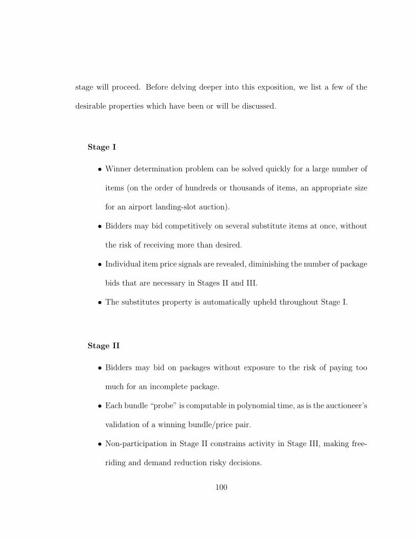
stage will proceed. Before delving deeper into this exposition, we list a few of the
desirable properties which have been or will be discussed.
Stage I
• Winner determination problem can be solved quickly for a large number of
items (on the order of hundreds or thousands of items, an appropriate size
for an airport landing-slot auction).
• Bidders may bid competitively on several substitute items at once, without
the risk of receiving more than desired.
• Individual item price signals are revealed, diminishing the number of package
bids that are necessary in Stages II and III.
• The substitutes property is automatically upheld throughout Stage I.
Stage II
• Bidders may bid on packages without exposure to the risk of paying too
much for an incomplete package.
• Each bundle “probe” is computable in polynomial time, as is the auctioneer’s
validation of a winning bundle/price pair.
• Non-participation in Stage II constrains activity in Stage III, making free-
riding and demand reduction risky decisions.
100
• A bidder may guarantee final possession of the package she is awarded at the
end of Stage II, but may be charged to beat out her Stage III competition.
Stage III
• If non-winning bids from Stage II can be combined to overcome a winning
package bid, this will be corrected in the final sealed-bid round.
• Competitive prices are determined which share the cost of displacement
among those who benefit, alleviating the free-rider problem.
4.3. Package Bidding and Probing
Preferences for complementary bundles introduce a potential for computa-
tional difficulty in the auction process. The problems of determining the winning
bids and prices for a given round of Stage I can be achieved in polynomial time, as
illustrated in Chapter 3. In order to develop Stage II, in which we wish to include
package bidding (for complementary packages), we must consider the computational
difficulties inherent when complements are introduced.
Consider scenarios in which bidders report demand correspondences (e.g. as
in Gul and Stacchetti [27] or Ausubel [2]). In these auctions each bidder reports
which bundles he would be willing to take at current prices (his demand correspon-
dence), after which the prices are changed, and the process repeated until a feasible
101
allocation exists. Both assume the gross substitutes property, but one might wonder
if their demand correspondence reporting technique might apply to a more general
model of bidders. The following theorem recognizes a difficulty in this scenario: with
a slightly general set of bidders not only is the overall problem of finding an efficient
allocation NP-hard, finding a feasible allocation for the subproblem at each round
is NP-complete.
Theorem 4.1. If the demand correspondence {∅, S} is admissible for any S ⊆ I,
then the problem of determining whether there exists a feasible allocation of items
among the bidders according to these reports is NP-complete.
Proof. The problem of allocating items according to demand correspondences is as
follows: given a set of demand correspondences D1, D2, ...DM , each a set of subsets
of the set of all items I, select one subset Sj from each Dj such that Sj ∩ Sj = ∅
whenever j 6= j and⋃
j∈J Sj = I.
It is easy to verify that this problem is in NP . Given a set of Sjs we need
only verify that Sj ∩ Sj = ∅ for all M(M−1)2
pairings of distinct bidders and that
⋃
j∈J Sj = I. Clearly these verifications can occur in polynomial time.
To show that the problem is NP-complete, we transform a generic set par-
titioning feasibility problem into an instance of the allocation feasibility problem.
Given a set of objects X and a family of subsets of X, F = {X1, X2, ...Xp}, the set
partitioning feasibility problem is to find a subset F ′ of F such that Xj ∩Xj = ∅ for
102
any distinct Xj and Xj in F ′and⋃
Xj∈F ′ Xj = X. To transform this into an instance
of the demand correspondence allocation feasibility problem simply let I = X and
create a bidder j for each Xj where j’s demand correspondence = {∅, Xj}. �
Though several theoretical treatments assume the gross substitutes condi-
tion, any extension of bidder preferences which allows for all-or-nothing bids may
expect computational difficulties. The following lemma implies that this compu-
tational difficulty does not occur when the gross substitutes condition holds, since
according to the lemma demand reports of the form {∅, S} cannot occur.
Lemma 4.2. If the gross substitutes condition holds, and a particular bidder de-
mands bundle S and the empty set at the current price, then the bidder demands
every subset S ′ ⊆ S at that price.
Proof. We make use of the assumptions that vj(∅) = 0 and vj(S) ≥ 0 ∀S ⊆ I, and
the property that a bidder’s net utility function is submodular given that the gross
substitutes condition holds [5]. Since Dj(p) ⊇ {∅, S} at the current price p, we have
uj(S, p) = uj(∅, p) = 0 ≥ uj(X, p) for any X ⊆ I. Submodularity is expressed by
uj(A, p) + uj(B, p) ≥ uj(A ∪ B, p) + uj(A ∩ B, p). Taking A = S ′ and B = S\S ′ we
have
uj(S′, p) + uj(S\S
′, p) ≥ uj(S, p) = 0
103
but since 0 ≥ uj(S′, p) and 0 ≥ uj(S\S
′, p), we must have uj(S′, p) = 0 and thus
S ′ ∈ Dj(p). �
Demand correspondence reporting can present a computational difficulty at
every round when the gross substitutes condition does not hold. Our overall approach
to an auction with complements is therefore as follows: use the bid-table format in
Stage I to enforce gross substitutes and reveal price information, and then accept
package bids on a basis which avoids the computational burden. The method for
avoiding this computational burden (until Stage III) is to only consider “strong”
bundle bids in Stage II, those which can immediately become winning without being
combined with the bundle bids of others.
Bidders in Stage II will “probe” various sets to determine whether they are
willing to place a “strong” bundle bid to compete for this set, or instead to indicate
that they have reached an upper bound on what they are willing to pay for this
set. For the first bidder in Stage II, this will proceed as described in the following
paragraph.
The bidder picks a set of items S which seems most attractive, using the
current prices as a first approximation of what bundle is most attractive. When the
bidder reports this set, the auctioneer (or an appropriately designed software pack-
age) probes it to determine a price. Since no other package bids have been accepted,
this task is equivalent to finding a price such that auction efficiency increases if the
104
package bid is accepted and the other items are awarded according to the reports
from Stage I. Let z∗ be the objective value from P at the end of Stage I, and let z−S
be a solution to the primal allocation problem P with the set of restrictions:
xijk = 0 ∀i, j, k with i ∈ S
The auctioneer may then report to the bidder a price of pS = z∗ − z−S + 1.
If the bidder is willing to pay this price, then auction efficiency is increased one
increment to z∗ + 1 by awarding S to this bidder at pS and awarding all other items
according to the assignment solution yielding z−S. Finding this assignment and
corresponding value of z−S is not computationally burdensome: we merely solve a
smaller assignment problem than was solved at each round of Stage I.
In order to continue this procedure past the first bidder in Stage II, we
must first define the set of packages for which package bids have been provisionally
accepted, S. Now, when a bidder probes set S, the auctioneer takes the current
auction value z∗, and computes z−S a solution to the primal allocation problem P
(from §3.2) with the set of restrictions:
xijk = 0 ∀i, j, k with i ∈ S or i ∈ T where T ∈ S with S ∩ T = ∅
105
The auctioneer reports a value pS = z∗ − z−S + 1 as before. If this price is
accepted, the new bid will push any overlapping bids out of the current allocation, so
that any items in a pushed out package bid but not in S must be allocated according
to the assignment information from Stage I. The bidder will pay the amount necessary
to compensate the auction for the drop in efficiency from displacing any currently
accepted package bids and reverting to bid table values for leftover items. Again the
computations are easily handled as restricted versions of the assignment problem
P. Since all such restrictions are simply bounds on the variables of P, the total
unimodularity of problem P, and hence polynomial solvability is not sacrificed.
In the Stage II package auction (as described until this point) there is a
potential exposure to inefficiency. A bidder may win a particularly desirable package
in Stage II but then also receive several other individual items from the collection
of items that were not awarded as part of a package. This will occur, for example,
if the bidder intends a slot in his package bid for a particular flight and then wins a
slot in the column corresponding to same flight in his bid table. This problem easily
disappears if we allow (or force) bidders to specify which of their agents (bid table
columns, flights) they plan to use the package of slots to satisfy, and simply removing
these columns from consideration in the calculation of z−S. This Package/Agent
Designation suggests a reasonable user-interface for Stage II probing; the bundle to
be probed may be specified by simply clicking on the bid table entry corresponding
106

to the row of the desired slot and the column of corresponding agent (flight) for each
slot in the bundle. The auctioneer removes the corresponding columns from the
bidder’s bid table until (perhaps) the bundle bid is no longer winning. This assures
that a bidder does not receive multiple slots for the same flight, even when package
bids are considered.
This removal of bid table columns suggests a further incentive to participa-
tion in the Dynamic Bid Table Auction of Stage I. As more packages are accepted
into the final allocation, more and more bid table columns are removed. Further,
certain slots may remain “loose,” not being incorporated in any package bid. As
fewer bid table columns remain active in the auction, competition on these loose
slots diminishes, resulting in lower final prices for slots that are won from bid table
entries. Intuitively, a bid table entry is very flexible and may be applied at any time;
by making this flexible offer to pay for an item in the early rounds a bidder may be
rewarded with a discounted price in the final allocation.
4.4. The Threshold Problem, the Free-Rider Problem and Efficiency
The auction format described in the present work differs from earlier com-
binatorial auction literature in its treatment of the threshold problem (as described
in §4.2). As mentioned above, some advocate a publicly available stand-by queue
of non-winning bids which an interested bidder may combine with her own to form
a winning bid (see [7][32]). We argue that this revelation of information is beyond
107
what is necessary to achieve efficiency and allows for tactical manipulation with little
if any benefit. As previously mentioned, this tactical manipulation comes in the form
of free-riding. A bidder with the ability to view the valuations of others will find it in
her best interests to reveal as little valuation as is necessary to form a winning bid,
placing as much burden as possible on those who have revealed their valuations to the
stand-by queue. Intelligent bidders may therefore cautiously shade down their own
revelation to the queue, possibly not revealing enough information for an efficient
allocation to be reached. Although we do not analyze this situation with rigorous
game-theory, it should be clear that the presence of the stand-by queue introduces
two potential problems associated with a disincentive to truthful revelation: bidders
taking advantage of the revealed information of others (free-riding) and the inability
to achieve efficiency due to cautious shading/free-riding defense strategies.
Even if for some altruistic reason we were to assume truthful revelation
(thereby nullifying the free-rider problem) another problem remains with the stand-
by queue approach. Maintaining the availability of this bid information throughout
the auction seems to diagnose the threshold problem as a barrier to bidding through-
out the auction, when in fact the threshold problem should be recognized as a barrier
to efficiency only in the final allocation. A bidder in an auction with a stand-by queue
may spend valuable computation time attempting to find a collection of available
108
queue bids to combine with his own, only to have the successfully combined coali-
tional bid knocked out in subsequent rounds. To clarify the situation, we advocate
a new definition of the threshold problem:
Definition: The Threshold Problem occurs when a collection of bids, each of which
cannot become winning unilaterally, can be combined to reach an efficient final allo-
cation.
There are two changes here from the definition given loosely in §4.2 (and in
the literature at large.) One distinction is the word “final” which makes it unneces-
sary in particular to consider a set of bids which may be combined to displace a bid
that eventually is not winning (as is the case in the intermediate phases of AUSM [7]
or PAUSE [32].) A second change is “each of which cannot become winning unilat-
erally.” If a bidder is willing to submit a bid which can become winning unilaterally,
we would want her to do so, rather than hiding this high valuation only to submit
this into the final sealed-bid phase when it is too late for her opponents to react.
To encourage revelation during Stage II we assume that a bidder has bid truthfully
and hold her to it in Stage III via bounds on her Stage III bids. These “honesty
constraints” make it risky to hide preferences in Stage II, as doing so will limit your
ability to bid aggressively in Stage III.
These observations suggest that the threshold problem should not be ad-
dressed until a final sealed-bid auction, regardless of what type of sealed-bid auction
109
is used. For the remainder of this section we describe the specific winner determina-
tion problem for a sealed-bid auction tailored to the multi-stage auction as developed
to this point. In particular, we want to maintain the bid table entries as bid informa-
tion, allow for package bidding, and uphold the flight designations for each package
bid as described in §4.3. We now describe an integer programming formulation for
determining winners, treating all revealed bid information as binding.
In addition to each (final) bid table entry bijk, we will have (from Stage
III) some indexed list of L package bids {(B1, S1), ...(Bl, Sl), ...(BL, SL)}, where each
(Bl, Sl) represents a bid of Bl for set Sl. This set of package bids will contain any
bid that is winning at the end of Stage II, and any other bids submitted for Stage
III after having been screened to ensure that each Bl could not become winning at
the end of Stage II. There is a natural OR relationship among the package bids of
the same bidder. It may be helpful to allow bidder the ability to express an XOR
relationship among a particular collection of bids, but since this may be handled
theoretically by the introduction of dummy items without changing the formulation
of P3 below, we currently ignore this consideration for the sake of simplicity.
We introduce the notation Al to denote the set of agents that a bidder has
associated with her particular package bid (Bl, Sl), and 0-1 decision variable yl which
equals one if and only if package bid (Bl, Sl) is accepted. In the following formulation
we will wish to express that if (Bl, Sl) is a winning package bid then the bid table
110
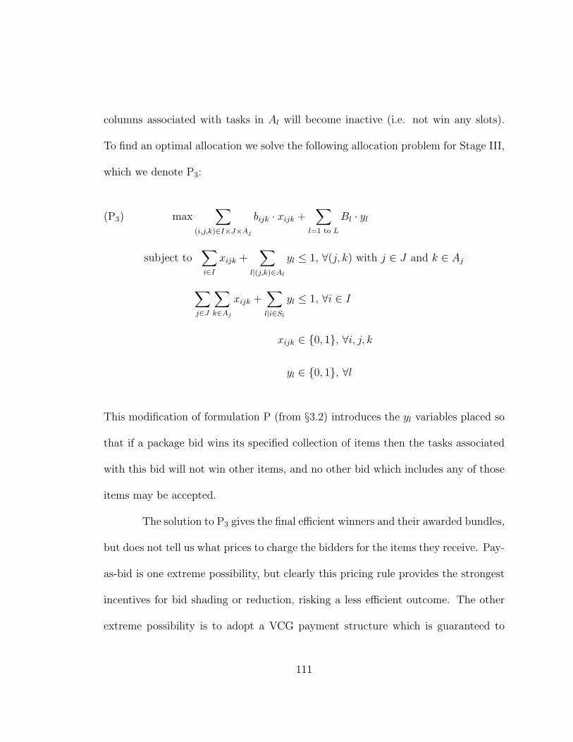
columns associated with tasks in Al will become inactive (i.e. not win any slots).
To find an optimal allocation we solve the following allocation problem for Stage III,
which we denote P3:
max∑
(i,j,k)∈I×J×Aj
bijk · xijk +∑
l=1 to L
Bl · yl(P3)
subject to∑
i∈I
xijk +∑
l|(j,k)∈Al
yl ≤ 1, ∀(j, k) with j ∈ J and k ∈ Aj
∑
j∈J
∑
k∈Aj
xijk +∑
l|i∈Sl
yl ≤ 1, ∀i ∈ I
xijk ∈ {0, 1}, ∀i, j, k
yl ∈ {0, 1}, ∀l
This modification of formulation P (from §3.2) introduces the yl variables placed so
that if a package bid wins its specified collection of items then the tasks associated
with this bid will not win other items, and no other bid which includes any of those
items may be accepted.
The solution to P3 gives the final efficient winners and their awarded bundles,
but does not tell us what prices to charge the bidders for the items they receive. Pay-
as-bid is one extreme possibility, but clearly this pricing rule provides the strongest
incentives for bid shading or reduction, risking a less efficient outcome. The other
extreme possibility is to adopt a VCG payment structure which is guaranteed to
111

be incentive compatible. There are, however, several problems with VCG payments
when superadditive valuations are present, as noted earlier. We instead terminate
our auction with a core outcome as advocated (for example) in the recent work
of Ausubel and Milgrom [5] and Hoffman et al [29]. The process we develop for
achieving these favorable outcomes is treated separately in Chapter 5, but before
doing so we explore the ideas of this chapter in greater depth by working through a
sample auction.
4.5. Example of a Schedule Auction for Airport Landing Slots
In this section we demonstrate the three-stage Schedule Auction with an
illustrative example. We assume a small auction environment for the sake of exposi-
tion, but one that is large enough to show some of the intricacies of the three-stage
format. We describe an auction with 5 airlines bidding for 10 airport landing slots.
For each of these bidding airlines, we introduce a sample strategy based on our
general assessments of the landing-slot application literature ([6],[21]) and a recent
workshop [49] on auctioning landing-slot rights. We work through the stages of the
auction, simulating participation with bidders behaving in a straightforward manner,
as described below. Before introducing the simulated bidding strategies in detail, we
discuss a few simple procedural measures to encourage participation in Stage I and
to avoid a monopoly situation.
112
To encourage participation in the Dynamic Bid Table Auction of Stage I, we
allow the auctioneer to make Package/Agent Designation (described in §4.3) manda-
tory in Stages II and III, and further stipulate that each Package/Agent Designation
must be composed of an assignment of the items in the package to agents using only
positive bid table entries. Thus, in Stages II and III a bidder can specify his package
of interest by highlighting positive bid entries in his bid table, with only one entry
per row and only one entry per column selected. This mandatory Package/Agent
Designation requires a bidder to keep at least one positive bid table entry in the row
of any item he may be interested in for the remainder of the auction. Further, if
he is interested in maintaining eligibility to win a package of size n, he must keep
at least one positive bid in at least n columns (i.e., for at least n agents). We note
that if a bidder decides to simply keep a single positive entry for each item, each
with its own dedicated agent, that he is essentially participating in a Simultaneous
Ascending Auction. The strength, however, of the bid table format is that the bidder
does not necessarily need to dedicate a single agent (column) to each item (row),
but may instead reduce his negative-synergy exposure by placing some bids in the
same column.
We note finally that this mandatory Package/Agent may be made even more
stringent (thus encouraging more revelation in Stage I) by replacing the requirement
of a positive bid entry with a requirement that each designated entry be above a
113
reservation value, perhaps one that is determined dynamically over the course of the
auction. This may take the form of a constraint saying that bid table entries less than
half of the final Stage I price for that row are ineligible for package designation, for
example. The auctioneer should be careful however that efficiency is not sacrificed
with too stringent a restriction, which could limit the behavior of a bidder with
very low individual item values but high positive synergy. In practice, this may be
avoided with an estimated upper bound on positive synergy, but for the example of
this section, we simply assume the weakest form of this restriction, that a bid table
entry must be positive to remain eligible for Package/Agent designation.
With mandatory Package/Agent Designation in place, any easy way to en-
force bundle-size limitations quickly presents itself. Since a bidder may not receive
any more items than he has bid table columns containing positive entries, the maxi-
mum bundle size is effectively constrained by the total number of bid table columns
allowed by the auctioneer. In the example of this section, the auctioneer stipulates
that no bidder may win more than 5 of the 10 available landing slots, and hence each
bid table can have only 5 columns.
We now describe the strategies of five simulated airlines, V , W , X, Y , and
Z. The items for auction are 10 landing slots at a particular airport between the
times of 1:00 PM and 3:15 PM on Fridays throughout an entire season. Because no
such auction has yet taken place (leaving us with no historical estimates of value),
114
the monetary units in our example are arbitrary. The final Stage I bid tables for
these airlines are collected in Figure 4.3 on page 116. We now describe the strategies
of each of our five fictional airlines.
Airline V: This airline represents a small carrier with simple preferences, that is
most interested in just buying its way into this market with one or two slots. As a
new entrant, this airline is unconcerned with which slots it receives, but would be
willing to pay at most 124 for one and most 224 for two slots. With these simple
preferences Airline V has no need for package bidding; its participation is complete
with the submission of its final bid table in Stage I (see Figure 4.3). Since this airline
is only interested in packages of two or fewer items, we see that only two of its bid
table columns contain positive entries.
Airline W: Similar to Airline V , Airline W is a small new entrant interested in two
or fewer time slots, and does not perceive any positive synergy among the items it
wins. This airline is, however, specifically interested in 1:00 or 1:15 landing slots and
experiences slowly accumulating costs of delay for later slots. These accumulating
costs of delay are evidenced by the decreasing columns of Airline W ’s bid table.
Airline X: This medium-sized airline is interested in purchasing at most four slots
to maintain the four flights it has historically landed in the 1:00-3:15 time frame.
It sets a maximum price for each slot in the historical landing time of each of the
115

Figure 4.3. An auction for airport time slots: Stage I. Winning entriesappear in bold, and prices are given by the displayed vector p
Airline V1 2 3 4 5
1:00 124 100
1:15 124 100
1:30 124 100
1:45 124 100
2:00 124 100
2:15 124 100
2:30 124 100
2:45 124 100
3:00 124 100
3:15 124 100
Airline W1 2 3 4 5
1:00 128 108
1:15 128 108
1:30 128 107
1:45 128 107
2:00 128 107
2:15 125 105
2:30 124 104
2:45 113 93
3:00 113 93
3:15 110 91
Airline X1 2 3 4 5
1:00
1:15
1:30 115
1:45 103 110
2:00 90 110 110
2:15 90 100 107
2:30 95 90
2:45 85 112
3:00 111
3:15 90
Airline Y1 2 3 4 5
1:00 107 107 107 87 87
1:15 114 114 114 94 94
1:30 120 120 120 100 100
1:45 114 114 114 94 94
2:00 107 107 107 87 87
2:15
2:30
2:45
3:00
3:15
Airline Z1 2 3 4 5
1:00 114 114 114
1:15 113 113 113
1:30
1:45
2:00 114 114 114
2:15 113 113 113
2:30
2:45
3:00 114 114 114
3:15 113 113 113
p =
1:00 108
1:15 108
1:30 115
1:45 108
2:00 108
2:15 107
2:30 104
2:45 104
3:00 104
3:15 104
116
corresponding flights, with decreasing bid table entries below, again reflecting accu-
mulating costs of delay. Unlike Airline W , Airline X will not settle for a slot that
is an hour or more after the targeted time slot for each flight, perhaps because this
would be too disruptive to its existing schedule or operational strategy. These pref-
erences are expressed with decreasing columns of at most four consecutive positive
entries in Airline X’s bid table. Further, based on previous experience, Airline X
calculates that it can save 21 monetary units in operational costs if three consecutive
slots are purchased. This may reflect, for example, an advantage in the scheduling of
ground crew, who would not sit idle if servicing consecutive slots. This expression of
positive synergy (21 units) cannot be conveyed in a bid table, but will help determine
Airline X’s package bids in Stages II and III.
Airline Y: This large incumbent airline has an established “banking” strategy in
which it lands several airplanes as close to 1:30 as possible, so that it may reorganize
its passengers for a round of outgoing flights taking off around 3:30 (after the slots of
this auction). It decides that slots after 2:00 arrive too late for outgoing passengers
on 3:30 flights, and so does not place any positive bids on the later slots. Airline Y
forecasts diminished revenue on the fourth and fifth flights landed in this time block,
but experiences economies-of-scale: 35 monetary units in operational savings for any
four flights landed in the 1:00 to 2:00 range, with an additional 1 unit of value if
the four slots are consecutive. Again, the diminished returns can be expressed with
117
reductions of the entries in the fourth and fifth columns of Airline Y ’s bid table,
while the positive-synergy bonus (from the economies-of-scale) must wait until Stages
II and III to be expressed.
Airline Z: Airline Z is medium-sized (demanding at most three slots) and has a
“shuttling” strategy. It would like to land one airplane every hour during this time
period, on the hour or just after. They calculate 34 additional monetary units of
benefit from any bundle giving them the ability to offer a reliable shuttle service
with three hourly landings during this time period. Further, it predicts greater ease
in advertising this service with landings specifically at 1:00 and 2:00, and perceive
3 additional units of synergy for any bundle allowing for the shuttle service and
containing both of these slots. This suggests several complementary bundles for this
bidder, with positive synergy that cannot be expressed in a bid table. Still, accord-
ing to the mandatory Package/Agent Designation, Airline Z must keep positive
bid table entries for all time slots of possible interest, while simultaneously keeping
positive bid entries in at three least columns to remain eligible for bundles of size
three.
Given the preferences described here, we now begin to run through the steps
of the three-stage Schedule Auction for this illustrative example. Each round of
Stage I proceeds with bidding airlines each submitting newly adjusted bid tables
based on the lowest Walrasian equilibrium prices announced by the auctioneer. It is
118
feasible that an airline knows what it wants its final entries to be and simply submits
its final bid table at the outset, but in general learning about the market prices will
guide the bidders through the process of writing their final bid table. We therefore
present only the final bid tables in Figure 4.3.
Although we do not present every step of Stage I for the sake of brevity, we
note that important learning may take place over the course of Stage I, providing
valuable information to the bidders and affecting their final bid tables. For example,
Airline V may have begun the auction with preferences for more than two landing
slots, but settled on two or fewer after the prices reached a certain level. At that
point they would stop bidding in their third, fourth, or fifth columns and allow those
entries to become inactive. For simplicity, however, we present these final bid tables
as if each airline had complete knowledge of its preferences and filled out its final bid
table accordingly. Thus, in order to focus on the flow of the entire Schedule Auction,
let us assume that Stage I has terminated with the final bid tables as given in Figure
4.3.
Comparing the bold winning entries in Figure 4.3 to the prices for the corre-
sponding items given by the vector p, we see that every item is awarded with positive
surplus (i.e., the price is always lower than the value of the winning entry). Each
bidding airline may compute its total current surplus (payments minus bids) to use
119
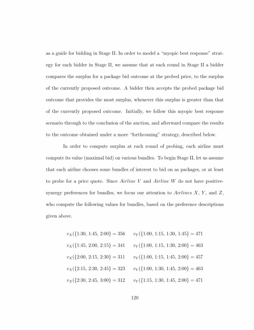
as a guide for bidding in Stage II. In order to model a “myopic best response” strat-
egy for each bidder in Stage II, we assume that at each round in Stage II a bidder
compares the surplus for a package bid outcome at the probed price, to the surplus
of the currently proposed outcome. A bidder then accepts the probed package bid
outcome that provides the most surplus, whenever this surplus is greater than that
of the currently proposed outcome. Initially, we follow this myopic best response
scenario through to the conclusion of the auction, and afterward compare the results
to the outcome obtained under a more “forthcoming” strategy, described below.
In order to compute surplus at each round of probing, each airline must
compute its value (maximal bid) on various bundles. To begin Stage II, let us assume
that each airline chooses some bundles of interest to bid on as packages, or at least
to probe for a price quote. Since Airline V and Airline W do not have positive-
synergy preferences for bundles, we focus our attention to Airlines X, Y , and Z,
who compute the following values for bundles, based on the preference descriptions
given above.
vX({1:30, 1:45, 2:00} = 356
vX({1:45, 2:00, 2:15} = 341
vX({2:00, 2:15, 2:30} = 311
vX({2:15, 2:30, 2:45} = 323
vX({2:30, 2:45, 3:00} = 312
vY ({1:00, 1:15, 1:30, 1:45} = 471
vY ({1:00, 1:15, 1:30, 2:00} = 463
vY ({1:00, 1:15, 1:45, 2:00} = 457
vY ({1:00, 1:30, 1:45, 2:00} = 463
vY ({1:15, 1:30, 1:45, 2:00} = 471
120

vZ({1:00, 2:00, 3:00} = 379
vZ({1:00, 2:00, 3:15} = 378
vZ({1:00, 2:15, 3:00} = 375
vZ({1:00, 2:15, 3:15} = 374
vZ({1:15, 2:00, 3:00} = 375
vZ({1:15, 2:00, 3:15} = 374
vZ({1:15, 2:15, 3:00} = 374
vZ({1:15, 2:15, 3:15} = 373
Under the assumption of myopic best response, we begin Stage II with
Airline X probing its bundles of interest to determine the current price for each. To
do so, the airline must designate a set of agents (flights) to be used with each package
so that the corresponding columns may be removed from its bid table. Throughout
all treatments in this section, we assume that each bidder designates agents to pack-
ages according to a maximum value assignment of the package to their bid table.
The results of Airline X’s probes in the first round are as follows.
Package Value Price Other items awarded Value Price Surplus
{1:30, 1:45, 2:00} 356 346 {2:45} 112 104 18
{1:45, 2:00, 2:15} 341 339 {2:45} 112 110 4
{2:00, 2:15, 2:30} 311 337 ∅ -26
{2:15, 2:30, 2:45} 323 330 ∅ -7
{2:30, 2:45, 3:00} 312 337 ∅ -25
121

We see that since some of Airline X’s bid table columns remain active he may receive
more items than just those in the package of interest, even when some columns are
removed to accommodate the package bid. We see that according to the probes only
two of these bundles would yield positive surplus for Airline X, and only one would
yield more surplus than the outcome at the termination of Stage I, which provided
Airline X with 10 units of surplus. Airline X therefore accepts the probed price
for the bundle {1:30, 1:45, 2:00}, which offers a better outcome than the Stage I
outcome in terms of surplus. Once a probed price/package is accepted, Airline X’s
turn is done, and the auction moves to the next randomly selected bidder’s turn to
probe. We assume that this random selection never gives the same bidder two turns
in a row, and includes all bidders in each round.
The collected results for Stage II of this auction (under the myopic best
response assumption) are tabulated in Figure 4.4. We assume that at each random-
ized round-robin turn each airline probes each bundle of interest, and accepts the
outcome with the highest surplus (for that airline) as long as that outcome pro-
vides more surplus than the current outcome (i.e., the one determined by the last
accepted probe). We show only the accepted package bid (if any) at each turn and
give the new surplus computed for Airlines X, Y , and Z after the acceptance and
reallocation, denoted sX , sY , and sZ , respectively.
122

Figure 4.4. Bundle probing in Stage II, assuming myopic best response
Bidder Accepted Bundle Price sX sY sZ
10 17 25Round 1 Z {1:00, 2:00, 3:00} 348 14 15 31
X {1:30, 1:45, 2:00} 346 18 6 27Y {1:00, 1:15, 1:30, 1:45} 461 6 10 21
Round 2 Z {1:00, 2:00, 3:00} 351 14 15 28X {1:30, 1:45, 2:00} 349 15 6 27Y {1:00, 1:15, 1:30, 1:45} 464 6 7 21
Round 3 X {1:30, 1:45, 2:00} 351 13 6 27Z {1:00, 2:15, 3:00} 345 17 6 30Y None accepted
Round 4 X None acceptedZ None accepted
Along the way, we observe some of the beneficial demand revelation proper-
ties of Stage II with a randomized round-robin bidding pattern. Particularly, since
we assume in this treatment that the only information bidders receive at each turn is
the price for probed bundles (i.e., they do not see what others win in their turns), it
is difficult for bidders to coordinate their bids to not interfere with one another. For
example, Airline X is only ever interested in its favorite package, {1:30, 1:45, 2:00},
for the entirety of the auction, because no other package ever maximizes surplus at
the probed prices. In Rounds 1 and 2, the randomized ordering places Airline Z
before Airline X, making it impossible for Airline Z to choose a non-interfering
bundle through probe prices alone. In Round 3, however, the randomization puts
Airline Z after Airline X, so that his Round 3 probes show a lower price for bun-
dles which do not conflict with Airline X. Airline Z is therefore able to achieve
123
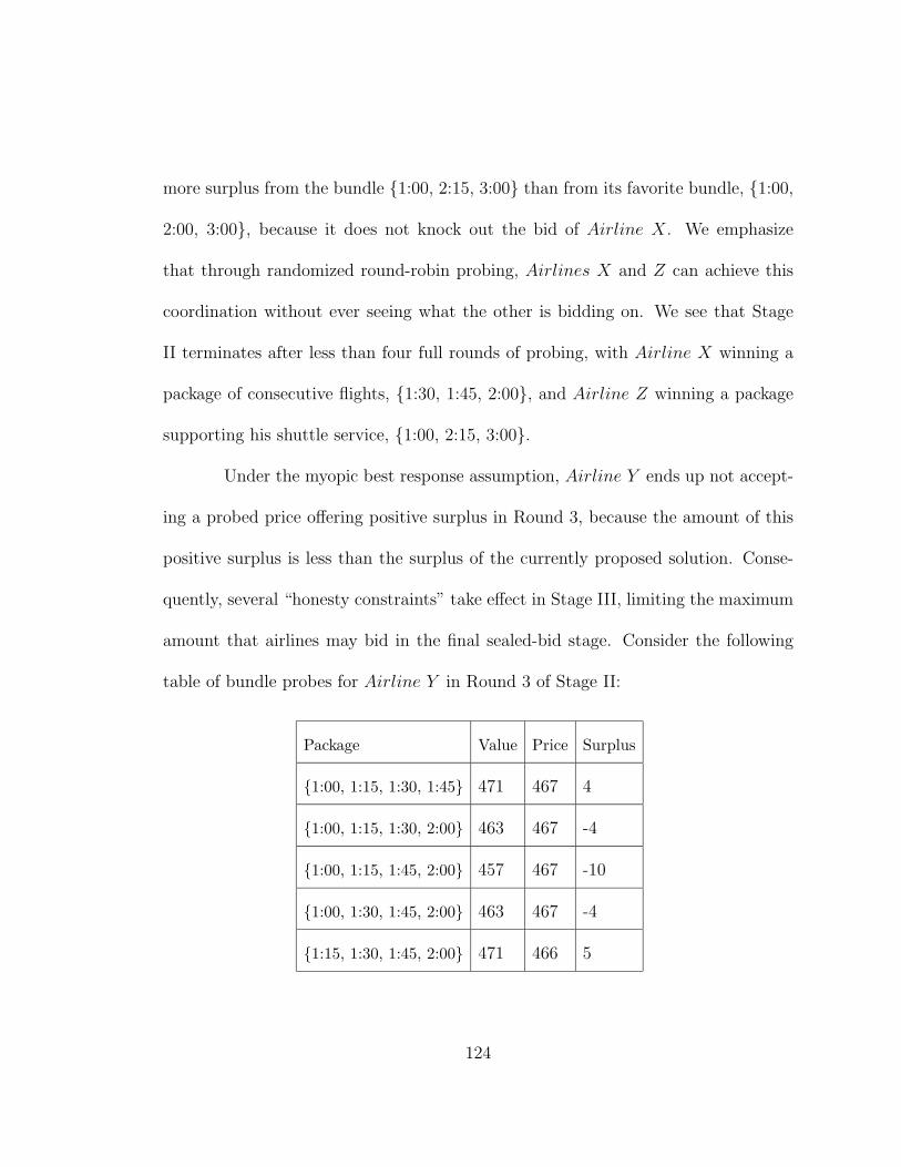
more surplus from the bundle {1:00, 2:15, 3:00} than from its favorite bundle, {1:00,
2:00, 3:00}, because it does not knock out the bid of Airline X. We emphasize
that through randomized round-robin probing, Airlines X and Z can achieve this
coordination without ever seeing what the other is bidding on. We see that Stage
II terminates after less than four full rounds of probing, with Airline X winning a
package of consecutive flights, {1:30, 1:45, 2:00}, and Airline Z winning a package
supporting his shuttle service, {1:00, 2:15, 3:00}.
Under the myopic best response assumption, Airline Y ends up not accept-
ing a probed price offering positive surplus in Round 3, because the amount of this
positive surplus is less than the surplus of the currently proposed solution. Conse-
quently, several “honesty constraints” take effect in Stage III, limiting the maximum
amount that airlines may bid in the final sealed-bid stage. Consider the following
table of bundle probes for Airline Y in Round 3 of Stage II:
Package Value Price Surplus
{1:00, 1:15, 1:30, 1:45} 471 467 4
{1:00, 1:15, 1:30, 2:00} 463 467 -4
{1:00, 1:15, 1:45, 2:00} 457 467 -10
{1:00, 1:30, 1:45, 2:00} 463 467 -4
{1:15, 1:30, 1:45, 2:00} 471 466 5
124
We see that two packages offer positive surplus, but neither offers more surplus
than the currently proposed outcome (following Z’s bid in Round 3) with surplus
of 6. Airline Y therefore does not accept any probed package bids in Round 3, in
accordance with our assumption of myopic best response.
Because of this non-acceptance, the honesty constraints dictate that no bun-
dle bid in Stage III may exceed the probed price for that bundle. Airline Y may
therefore not submit a bid higher than 467 on the bundle {1:00, 1:15, 1:30, 1:45}, nor
a bid higher than 466 on the bundle {1:15, 1:30, 1:45, 2:00}. Indeed, according to
the honesty constraints Airline Y may not bid higher than 467 on the bundle {1:00,
1:15, 1:45, 2:00}, for example, but since this bound exceeds Airline Y ’s valuation
for this bundle, the constraint will not be restrictive.
Figure 4.5 shows the results of the entire auction at each stage, assuming
myopic best response in Stage II. We assume that each bidder bids honestly on
bundles in Stage III, except where this would violate the honesty constraints. The
general method used to compute the final (bidder-Pareto-optimal core) payments is
given in Chapter 5. This method assures that the payment mechanism corresponds
to the VCG outcome whenever that outcome is in the core, and takes the minimal-
payment core outcome closest to the VCG outcome otherwise. This approximation of
the VCG outcome reinforces our assumption of honest submission of package values
in Stage III. For the results of this section, the algorithm does terminate at the VCG
125

Figure 4.5. Results for all Stages, assuming myopic best response inStage II
Stage I Bidder Bundle Value Payment Surplus
V {2:30} 124 104 20
W {1:00} 128 108 20
X {2:00, 2:45} 222 212 10
Y {1:15, 1:30, 1:45} 348 331 17
Z {2:15, 3:00, 3:15} 340 315 25
totals 1162 1070 92
Stage II Bidder Bundle Value Payment Surplus
V {3:15} 124 91 33
W {2:30} 124 100 24
X {1:30, 1:45, 2:00, 2:45} 468 451 17
Y {1:15} 114 108 6
Z {1:00, 2:15, 3:00} 375 345 30
totals 1205 1095 110
Stage III Bidder Bundle Value Payment Surplus
V {3:00} 124 102 22
W {2:30} 124 102 22
X {2:45} 112 100 12
Y {1:00, 1:30, 1:45, 2:00} 463 460 3
Z {1:15, 2:15, 3:15} 373 321 52
totals 1196 1085 111
outcome, since it does happen to be in the core, allowing the avid reader to verify the
results of this section on her own, with no need to skip ahead to the more advanced
technique described in Chapter 5.
Observing Figure 4.5, we see that total value (for all bidders) increases from
the end of Stage I to the end of Stage II, but drops from the end of Stage II to the
Stage III final outcome. This forces to ask, why would the auction pick an outcome
with lower total value given more bid information in Stage III? The answer is that
126
due to the nature of probe pricing in Stage II and honesty constraints in Stage
III, some of the values for various bundles remain hidden from the auctioneer. For
example, in Stage II the auctioneer cannot be sure that any bidder values a particular
bundle more than the price they have accepted for that bundle. The auctioneer could
therefore only know that Airline X’s value for its awarded bundle at the end of Stage
III is at least 463 (the price of the bundle bid, 351, plus the known value from the
bid table entry of 112), but cannot tell that Airline X actually values the bundle
at 468. Similarly, because of honesty constraints Airline Z can bid at most 364 for
its awarded bundle in Stage III, so some of Airline Z’s value for this bundle (373)
remains hidden from the auctioneer. We therefore compute the total perceived value
to be 1162, 1170, and 1187, for Stages I, II and III, respectively. Thus as far as the
auctioneer can tell, perceived value (as opposed to actual value as shown in Figure
4.5) is increasing from each stage to the next.
We see also (in the instance of Figure 4.5) that total payments and surplus
are increasing from the end of Stage I to the end of Stage II. Indeed, payments must
increase from the Stage I outcome to the Stage II outcome; they increase by one
increment for every package bid accepted. (We do not discuss increment size for
Stage II here, though it may be fined tuned in practice to speed up or slow down the
pace of the auction.) It should be remembered, however, that payments in Stages I
and II are merely price signals, and that final payments may be higher or lower than
127

as signaled in earlier stages. Payments may seem to rise from Stage II to III since
more demand and hence more price competition has been revealed. This is the case
for small entrant Airlines V and W , who saw good prices on a single item rise in
Stage III. Airline Z provides an example of the opposite possibility; the price signals
from Stage II (which measure a minimum unilateral payment) can overestimate the
payment that is needed by the end of the auction, especially if the package bid can be
coordinated with those of others. Overall, in this instance total payments dropped
from Stage II to Stage III, though our experience with other examples (not discussed
in this text) show that this may not always be the case.
The Schedule Auction is designed with honesty constraints to encourage
demand revelation in Stage II, and a bidder-Pareto-optimal pricing rule in Stage III
to minimize the costs of this demand revelation (in terms of increased payments) as
much as possible. Do the honesty constraints work? Would it have been a better
idea for the bidders to play a more forthcoming strategy (revealing more demand)
in Stage II? We now demonstrate the possibility that no bidder is made worse off if
the myopic best response strategy is replaced by a more truthful strategy.
To demonstrate this interesting possibility, let us return to the end of Stage
I (i.e., the bids of Figure 4.3) and re-run the auction with the assumption of a more
forthcoming set of bidders in Stage II. In particular, we say that a “forthcoming”
bidder accepts the probed package bid outcome that provides him the most surplus,
128
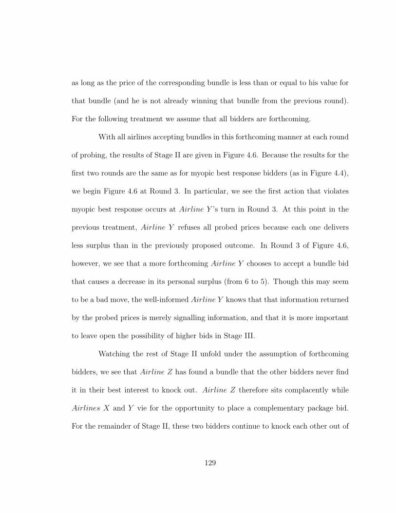
as long as the price of the corresponding bundle is less than or equal to his value for
that bundle (and he is not already winning that bundle from the previous round).
For the following treatment we assume that all bidders are forthcoming.
With all airlines accepting bundles in this forthcoming manner at each round
of probing, the results of Stage II are given in Figure 4.6. Because the results for the
first two rounds are the same as for myopic best response bidders (as in Figure 4.4),
we begin Figure 4.6 at Round 3. In particular, we see the first action that violates
myopic best response occurs at Airline Y ’s turn in Round 3. At this point in the
previous treatment, Airline Y refuses all probed prices because each one delivers
less surplus than in the previously proposed outcome. In Round 3 of Figure 4.6,
however, we see that a more forthcoming Airline Y chooses to accept a bundle bid
that causes a decrease in its personal surplus (from 6 to 5). Though this may seem
to be a bad move, the well-informed Airline Y knows that that information returned
by the probed prices is merely signalling information, and that it is more important
to leave open the possibility of higher bids in Stage III.
Watching the rest of Stage II unfold under the assumption of forthcoming
bidders, we see that Airline Z has found a bundle that the other bidders never find
it in their best interest to knock out. Airline Z therefore sits complacently while
Airlines X and Y vie for the opportunity to place a complementary package bid.
For the remainder of Stage II, these two bidders continue to knock each other out of
129
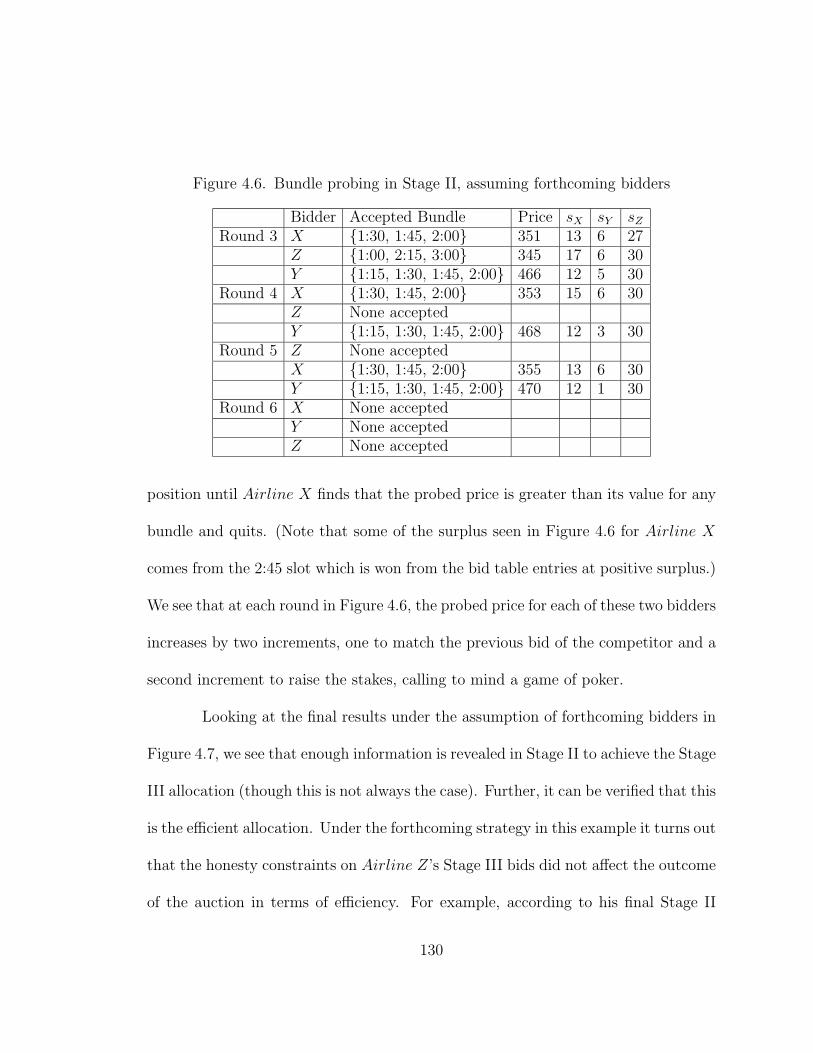
Figure 4.6. Bundle probing in Stage II, assuming forthcoming bidders
Bidder Accepted Bundle Price sX sY sZ
Round 3 X {1:30, 1:45, 2:00} 351 13 6 27Z {1:00, 2:15, 3:00} 345 17 6 30Y {1:15, 1:30, 1:45, 2:00} 466 12 5 30
Round 4 X {1:30, 1:45, 2:00} 353 15 6 30Z None acceptedY {1:15, 1:30, 1:45, 2:00} 468 12 3 30
Round 5 Z None acceptedX {1:30, 1:45, 2:00} 355 13 6 30Y {1:15, 1:30, 1:45, 2:00} 470 12 1 30
Round 6 X None acceptedY None acceptedZ None accepted
position until Airline X finds that the probed price is greater than its value for any
bundle and quits. (Note that some of the surplus seen in Figure 4.6 for Airline X
comes from the 2:45 slot which is won from the bid table entries at positive surplus.)
We see that at each round in Figure 4.6, the probed price for each of these two bidders
increases by two increments, one to match the previous bid of the competitor and a
second increment to raise the stakes, calling to mind a game of poker.
Looking at the final results under the assumption of forthcoming bidders in
Figure 4.7, we see that enough information is revealed in Stage II to achieve the Stage
III allocation (though this is not always the case). Further, it can be verified that this
is the efficient allocation. Under the forthcoming strategy in this example it turns out
that the honesty constraints on Airline Z’s Stage III bids did not affect the outcome
of the auction in terms of efficiency. For example, according to his final Stage II
130
Figure 4.7. Results for all Stages, assuming forthcoming bidders inStage II
Stage I Bidder Bundle Value Payment Surplus
V {2:30} 124 104 20
W {1:00} 128 108 20
X {2:00, 2:45} 222 212 10
Y {1:15, 1:30, 1:45} 348 331 17
Z {2:15, 3:00, 3:15} 340 315 25
totals 1162 1070 92
Stage II Bidder Bundle Value Payment Surplus
V {3:15} 124 91 33
W {2:30} 124 100 24
X {2:45} 112 100 12
Y {1:15, 1:30, 1:45, 2:00} 471 470 1
Z {1:00, 2:15, 3:00} 375 345 30
totals 1206 1106 100
Stage III Bidder Bundle Value Payment Surplus
V {3:15} 124 91 33
W {2:30} 124 100 24
X {2:45} 112 100 12
Y {1:15, 1:30, 1:45, 2:00} 471 464 7
Z {1:00, 2:15, 3:00} 375 317 58
totals 1206 1072 134
probes, Airline Z may not bid more than 361 for the bundle {1:00, 2:00, 3:00}, even
though its true value for this bundle is 379. Airline Z was therefore able to hide some
of his value for bundles (even from the auctioneer) without consequence, a beneficial
privacy-preservation property. More importantly, comparing Figure 4.7 with Figure
4.5, we see that no bidder strictly prefers the myopic best response outcome to the
forthcoming outcome, with only Airline X being indifferent between the two. This
131
comparison illustrates the strength of honesty constraints for encouraging demand
revelation for complementary bundles.
With this example we conclude our discussion of Schedule Auctions, and
move on to discuss the calculation of bidder-Pareto-optimal core prices performed in
Stage III. We treat this new computational technique separately in Chapter 5, since
it may be applied in a more general combinatorial auction setting.
132
CHAPTER 5
Generation and Selection of Core Outcomes
Definition: Let an outcome, Γ, refer to an allocation and set of payments for bidders
in a combinatorial auction. Let the coalition, CΓ, refer to the set of bidders receiving
items under outcome Γ.
Perhaps the most obvious problem with VCG payments in terms of ex-
post satisfaction is that the VCG outcome may not be a “core outcome”. The
core conditions for a one-sided (forward) auction may be stated by the following
definitions, where bidder j weakly prefers outcome Γ1 to Γ2 if Γ1 provides bidder j
with utility greater than or equal to the utility of outcome Γ2.
Definition: An outcome Γ is blocked if there is an alternative outcome ΓB which
generates strictly greater revenue for the seller and for which every bidder in CΓB
weakly prefers ΓB to Γ. CΓBmay be referred to as a blocking coalition.
Definition: An outcome Γ that is not blocked is called a core outcome.
It is well known that a VCG outcome may not be a core outcome. Consider
the following three-bidder, two-item example from Ausubel [2]. Let b1({A,B}) =
b2({A}) = b3({B}) = 2. In the efficient allocation, bidder 2 wins item A while bidder
3 wins item B. VCG payments for each winning bidder are easily computed to be
133

zero. This is not a core outcome because bidder 1 would prefer to pay any amount
up to 2 units to receive both items, an outcome which is clearly more desirable to
the seller. If instead bidders 2 and 3 each pay 1, the coalition containing just bidder
1 no longer blocks, and the outcome is in the core.
As an alternative to VCG pricing, Ausubel and Milgrom [5] suggest an as-
cending proxy auction which arrives at a more desirable core outcome. DeVries,
Schummer and Vohra [17] interpret this algorithm for winner/payment determi-
nation as a subgradient algorithm: at each moment in the process the algorithm
determines a revenue maximizing allocation given some current set of prices, and a
net utility maximizing bundle for each bidder. Each non-anonymous bundle price
is then adjusted up by one increment for each bundle that is not contained in the
“seller’s choice” allocation. This process corresponds to incremental stepping in the
direction of a subgradient. As is commonly the case with the subgradient algorithm,
convergence may be slow and depends critically on the choices of step size.
Experimental evidence supporting this characterization of the ascending
proxy auction as slow to converge is given by Hoffman et al [29], who also suggest
methods for accelerating the convergence of the procedure. Given that the proxy
information is available to the auctioneer for use in an integer programming formu-
lation, they suggest that several instances of the winner determination problem be
solved to determine an efficient allocation and VCG prices. The VCG prices are then
134
used as starting prices for winning bundles in the ascending proxy auction. The bids
of losing bidders can be priced at the submitted value, while non-winning bundles of
winning bidders can start at an initial price equal to their value (as entered into the
proxy) minus the current surplus (i.e. bid minus payment) on that bidder’s winning
bundle. The ascending proxy auction then proceeds as described by Ausubel and
Milgrom [5], but now from a better starting point determined by solving at most
min(N,M) + 1 winner determination problems.
We suggest an alternative to this accelerated proxy auction using a constraint
generation technique. Starting at the VCG payments as in [29], we wish to achieve
a “bidder-Pareto-optimal core outcome.” Noting that the core region in payment
space can be defined by an exponential number of linear constraints (one for each
coalition C ⊆ J = {1, ...M}), we are motivated to generate the constraints only when
they are violated for a given payment vector, rather than applying all constraints
to define the core region as in Parkes [54]. To do this, we formulate the separation
problem for core constraints (problem SEPt in §5.1), an IP which can be solved to
find the most violated constraint. Payments are then adjusted by solving an LP
with constraints added from each solution of SEPt. When no new constraints can
be generated, the procedure terminates at a core outcome.
The desirable bidder-Pareto-optimal core outcome obtained by the accel-
erated proxy method [29] is indeed the payment structure we achieve using the
135
technique of this chapter. Though this method is proposed to determine the final
payments in the three-stage auction of Chapter 4, we advocate this outcome for any
sealed-bid combinatorial auction. Any payment/allocation that is not in the core is
susceptible to the complaints of dissatisfied bidders, while a core outcome is bidder-
Pareto-optimal if there is no other core outcome weakly preferred by every winning
bidder. Whenever the VCG outcome is not in the core, the bidder-Pareto-optimal
core outcome discourages bid reduction by minimizing total payments, and corre-
sponds exactly to the VCG outcome whenever it is in the core. As our technique
is proposed for a general combinatorial auction scenario, we maintain an XOR of
flat bids language (with an exclusive bid for any bundle) throughout this chapter,
allowing for a direct comparison to the work of Hoffman et al [29] and others.
5.1. Core Constraint Generation
As in Hoffman et al [29], our general approach is to first solve several winner
determination problems for a sealed-bid combinatorial auction, settling on a partic-
ular set of winning bidders and VCG payments. Given this fixed outcome ΓV CG we
denote the associated coalition of winners as W = CΓV CGand the associated pay-
ments πV CGj for each bidder j ∈ W . Starting from this VCG outcome, we wish to
arrive at a bidder-Pareto-optimal core outcome with the same efficient allocation;
only payments will differ between the VCG outcome and the final core outcome
proposed here.
136

From a constrained optimization point of view it is difficult to categorize the
bidder-Pareto-optimal core payments for two reasons. First, an exponential number
of possible coalitions must be considered to define the core region in payment space.
Secondly, it is difficult to gauge how much a winning bidder will contribute to a
“coalitional value function” without knowledge of her final payment.
Given our definition of the core, it seems convenient to define a core con-
straint for any blocking outcome Γ as∑
j∈W πj ≥ zCΓ, where πj is a payment made
by each bidder j ∈ W , and zC is the coalitional value of C. We define this coalitional
value zC as the maximum total payments that a coalition C would be willing to offer
the seller in any outcome Γ with CΓ = C. This formulation of a core constraint
emphasizes that any offer that could be made by a coalition must be matched by
the set of winning bidders. With every coalition defining a constraint of this form,
we suggest our first characterization of the core:
∑
j∈W
πj ≥ zC , ∀C ⊆ J(CORE1)
πV CGj ≤ πj ≤ bj(Sj), ∀j ∈ W
Defining the core points in payment space with linear constraints gets us closer to
computing the bidder-Pareto-optimal core payments using an LP, and allows us to
restate our two difficulties from above:
137
• Noting the exponential number of constraints in CORE1, how do we sep-
arate which constraints must be applied from those that can be ignored
without consequence?
• How do we compute the value of zC for a particular coalition C?
To appreciate the subtlety of the second question, observe that given a can-
didate payment vector πt, any bidder j ∈ W would not want to join a coalition
and receive less surplus than she would at her current payment πtj. Trying to solve
the winner determination problem restricted to the bidders in the coalition C there-
fore overstates the amount that any winning bidder in C would contribute to the
coalitional value zC , because she will not be compensated her opportunity cost (the
amount of surplus she stands to gain at the current vector of payments). The re-
sult would be the application of a too restrictive constraint, therefore charging the
winning bidders too much. We must instead consider that each winning bidder’s
opportunity cost limits her contribution to a blocking coalition. We therefore amend
our notation to capture the fact that a coalitional value function depends on a pay-
ment vector π, and thus change to zC(π).
We may now describe our general iterative approach as follows: at a current
vector in payment space, πt at each discrete iteration t, find the coalition Ct with the
highest coalitional value relative to current payments, zC(πt). If this coalition blocks
the currently proposed allocation (the efficient solution with payments πt), apply the
138

corresponding core constraint and find a new bidder-Pareto-optimal payment πt+1. If
this coalition does not block then terminate at the currently proposed outcome (since
it satisfies all core constraints). Before demonstrating this technique in full detail,
we observe a few basic properties of each winning bidder’s “coalitional contribution”
relative to current payments, leading us to a more useful LP characterization than
that of CORE1.
Let Sj be the bundle awarded to winning bidder j in the efficient solution.
Relative to the current payment vector, bidder j would not voluntarily join a coalition
that offers him less surplus than bj(Sj) − πtj, his opportunity cost. If a coalition
provides bidder j with bundle Sj (possibly the same as Sj, but in general not) then
bidder j would contribute at most bj(Sj) − (bj(Sj) − πtj) into the coalition value
function; if he contributed more, then he would perceive less benefit (surplus) from
the hypothetical outcome of the coalition then the one proposed by the auctioneer
at iteration t. If bidder j is not in the set W , there is no opportunity cost to recover,
and he would offer his entire value for a bundle in an effort to block the set of winning
payments. In this case bj(Sj = ∅) = πtj = 0 and his coalitional contribution would
be bj(Sj). In general we have the following definition:
Definition: Facing payment of πtj for bundle Sj in the efficient allocation, bidder j
would be willing to make a coalitional contribution of qj(C, πtj) = bj(Sj)− bj(Sj)+πt
j
to receive Sj as part of the coalition C.
139
Lemma 5.1. We note the following basic properties of the coalitional contribution
qj(C, πtj):
(1) If bidder j were to pay an amount πCj that is greater than qj(C, πt
j) to join
coalition C and win Sj, then bidder j would experience less surplus from
the coalition than from the auctioneer’s proposed outcome Sj with payment
πtj
(2) qj(C, πtj) increases linearly in πt
j, ∀j ∈ W
(3) ∀j ∈ J , Sj = Sj implies that qj(C, πtj) = πt
j
(4) qj(C, πtj) = bj(Sj) and j ∈ W ∩ C imply that πt
j = bj(Sj)
(5) qj(C, πtj) = bj(Sj), ∀j /∈ W
Proof. Property (1) verifies that our definition of the quantity qj(C, πtj) truly reflects
what we mean by coalitional contribution, and follows from the definition: πCj >
qj(C, πtj) = bj(Sj) − bj(Sj) + πt
j implies that surplus from the coalitional outcome is
bj(Sj)−πCj < bj(Sj)−πt
j, where the right-hand-side of the last inequality is exactly the
surplus from the auctioneer’s outcome. Properties (2), (3), and (4) follow directly
from the definition while Property (5) follows from the standard assumption that
bj(∅) = 0 ∀ j, and thus πtj = 0 ∀j /∈ W . �
Now that we have established the importance of opportunity cost and shown
that bidder j’s coalitional contribution will normally be less than her value for the
bundle given to her by the coalition, we now formulate the core-constraint separation
140

problem at payment vector πt. At any point in payment space, πt, the integer
program SEPt finds the most violated core constraint, or tells us that no blocking
coalition can be found.
z(πt) = max∑
j∈J
∑
S⊆I
bj(S) · xj(S) −∑
j∈W
(bj(Sj) − πtj) · γj(SEPt)
subject to∑
S⊇{i}
∑
j∈J
xj(S) ≤ 1, ∀i ∈ I
∑
S⊆I
xj(S) ≤ 1, ∀j ∈ J\W
∑
S⊆I
xj(S) ≤ γj, ∀j ∈ W
xj(S) ∈ {0, 1}, ∀S ⊆ I, ∀j ∈ J
γj ∈ {0, 1}, ∀j
The added terms in the objective of this IP formulation (starting from a general XOR
winner determination problem) ensure that any winning bidder will be compensated
his opportunity cost if selected. It is easy to verify that any bidder j ∈ J contributes
exactly qj(C, πtj), his coalitional contribution.
If the objective z(πt) >∑
j∈W πtj then the bidders for which xj(S) = 1 form
a coalition Ct which blocks the efficient allocation with the current set of payments;
i.e. Ct is a set of bidders such that z(πt) = zCt(πt). If z(πt) =∑
j∈W πtj then we
141
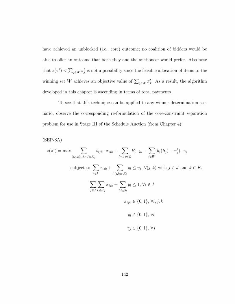
have achieved an unblocked (i.e., core) outcome; no coalition of bidders would be
able to offer an outcome that both they and the auctioneer would prefer. Also note
that z(πt) <∑
j∈W πtj is not a possibility since the feasible allocation of items to the
winning set W achieves an objective value of∑
j∈W πtj. As a result, the algorithm
developed in this chapter is ascending in terms of total payments.
To see that this technique can be applied to any winner determination sce-
nario, observe the corresponding re-formulation of the core-constraint separation
problem for use in Stage III of the Schedule Auction (from Chapter 4):
z(πt) = max∑
(i,j,k)∈I×J×Kj
bijk · xijk +∑
l=1 to L
Bl · yl −∑
j∈W
(bj(Sj) − πtj) · γj
(SEP-SA)
subject to∑
i∈I
xijk +∑
l|(j,k)∈Kl
yl ≤ γj, ∀(j, k) with j ∈ J and k ∈ Kj
∑
j∈J
∑
k∈Kj
xijk +∑
l|i∈Sl
yl ≤ 1, ∀i ∈ I
xijk ∈ {0, 1}, ∀i, j, k
yl ∈ {0, 1}, ∀l
γj ∈ {0, 1}, ∀j
142

Comparing with the Stage III winner determination problem P3 from Chapter 4, we
see again that the core-constraint separation problem is simply the winner determi-
nation problem augmented with opportunity costs for each bidder j that must be
deducted from the objective function whenever j belongs to the coalition implied by
a feasible solution. In general, this can be implemented for any combinatorial auc-
tion with an IP winner determination problem by at worst including constraints of
the form xj ≤ γj for every decision variable xj signifying the allocation of an item to
bidder j. In both SEPt and SEP-SA, however, our formulations make more efficient
use of the γj variables by placing them within existing constraints. In any case, one
can employ some version of the core-constraint separation problem to determine a
maximally violated blocking coalition Ct.
Having found a coalition Ct that blocks the proposed outcome with payment
vector πt, we know that the constraint∑
j∈W πj ≥ zCt(π) is violated for the current
payment vector. One way to characterize the set of core payments is therefore as
the set of points in payment space that satisfy the constraints formulated above as
CORE1. The region defined by CORE1, however, is difficult to generate or optimize
over because there are an exponential number of constraints in the first set and each
has a right-hand-side requiring optimization of an NP-hard winner determination
problem to compute. In addition, Property (2) from Lemma 5.1 indicates that price
increases on any bidder j ∈ W ∩C completely cancel with the corresponding increase
143

in coalitional contribution qj(C, πtj) on the right-hand-side of the constraint for C in
CORE1.
Consequently, our method is to find bidder-Pareto-optimal core payments
by generating core constraints of the form∑
j∈W\Ct πj ≥ z(πt) −∑
j∈W∩Ct πtj. The
right-hand-side of these constraints are computed once and remain constant for the
remainder of the algorithm, unlike the right-hand-side of the constraints in CORE1.
In economic terms, we choose these constraints because they do not hold winning
bidders in a blocking coalition Ct responsible for overcoming coalition Ct, the futility
of which is clear by our formulation of coalitional contribution. We also note that
these constraints are equivalent to those defined as core constraints in Parkes [54]
and Hoffman et al [29] through a linear change of variables.
After finding each of these constraints using SEPt, we may solve the following
linear program BPOt to find a set of bidder-Pareto-optimal core payments, in the
core relative to all coalitions found through iteration t:
θt = min∑
j∈W
πj(BPOt)
subject to∑
j∈W\Cτ
πj ≥ z(πτ ) −∑
j∈W∩Cτ
πτj , ∀τ ≤ t(CORE2)
πV CGj ≤ πj ≤ bj(Sj), ∀j ∈ W
144
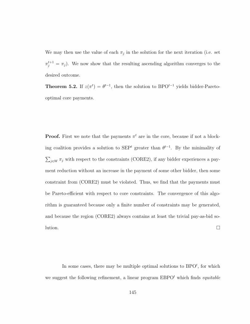
We may then use the value of each πj in the solution for the next iteration (i.e. set
πt+1j = πj). We now show that the resulting ascending algorithm converges to the
desired outcome.
Theorem 5.2. If z(πt) = θt−1, then the solution to BPOt−1 yields bidder-Pareto-
optimal core payments.
Proof. First we note that the payments πt are in the core, because if not a block-
ing coalition provides a solution to SEPt greater than θt−1. By the minimality of
∑
j∈W πj with respect to the constraints (CORE2), if any bidder experiences a pay-
ment reduction without an increase in the payment of some other bidder, then some
constraint from (CORE2) must be violated. Thus, we find that the payments must
be Pareto-efficient with respect to core constraints. The convergence of this algo-
rithm is guaranteed because only a finite number of constraints may be generated,
and because the region (CORE2) always contains at least the trivial pay-as-bid so-
lution. �
In some cases, there may be multiple optimal solutions to BPOt, for which
we suggest the following refinement, a linear program EBPOt which finds equitable
145
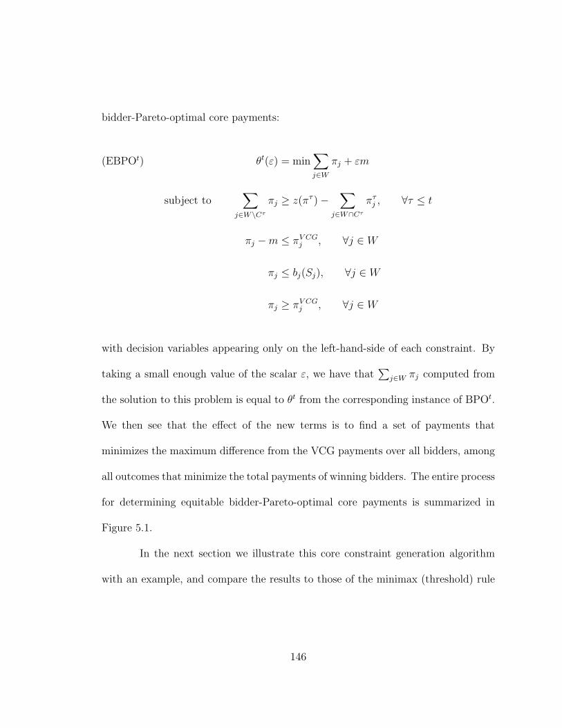
bidder-Pareto-optimal core payments:
θt(ε) = min∑
j∈W
πj + εm(EBPOt)
subject to∑
j∈W\Cτ
πj ≥ z(πτ ) −∑
j∈W∩Cτ
πτj , ∀τ ≤ t
πj − m ≤ πV CGj , ∀j ∈ W
πj ≤ bj(Sj), ∀j ∈ W
πj ≥ πV CGj , ∀j ∈ W
with decision variables appearing only on the left-hand-side of each constraint. By
taking a small enough value of the scalar ε, we have that∑
j∈W πj computed from
the solution to this problem is equal to θt from the corresponding instance of BPOt.
We then see that the effect of the new terms is to find a set of payments that
minimizes the maximum difference from the VCG payments over all bidders, among
all outcomes that minimize the total payments of winning bidders. The entire process
for determining equitable bidder-Pareto-optimal core payments is summarized in
Figure 5.1.
In the next section we illustrate this core constraint generation algorithm
with an example, and compare the results to those of the minimax (threshold) rule
146

Figure 5.1. The Core Constraint Generation Algorithm
Initialize: Iteratively solve the Winner Determination Problem, findingwinners W and VCG payments; Set t = 1, π1 = πV CG,and θ0(ε) =
∑
j∈W πV CGj
Iteration t: Solve SEPt
If z(πt) > θt−1(ε)Add constraint
∑
j∈W\Ct πj ≥ z(πt) −∑
j∈W∩Ct πtj
to EBPOt and solve, updating θt(ε).Set πt+1
j = πj, the values found from EBPOt.Iterate: t = t + 1
ElseTerminate
for one-sided auctions as discussed by Parkes [54] and to the examples presented in
Hoffman et al [29].
5.2. Examples and Comparison to the MiniMax Rule
To illustrate our technique for determining bidder-Pareto-optimal core out-
comes using core constraint generation, consider the three-item, eight-bidder example
of Figure 5.2. Here we depict the three items as pieces of a pie to indicate visually
which bids are on which items. Inspection shows that bidders 1, 2, and 3 constitute
the set of winners in the efficient allocation, as indicated. In accord with our earlier
notation we will say that W = {1, 2, 3}.
147

Figure 5.2. An auction for which threshold payments do not minimizetotal payments
With the set of winners determined, we next compute πV CG1 = πV CG
2 =
πV CG3 = 10, and so set π1
1 = π12 = π1
3 = 10. Solving SEP1 the separation problem at
iteration 1, we find the most violated blocking coalition C1 = {3, 4} with z(π1) =
38 > 30 =∑
j∈W π1j . We then add the constraint π1 + π2 ≥ 28 to the formulation
EBPO1 and solve to find the new set of payments π21 = π2
2 = 14, π23 = 10. Next
we solve SEP2 and find that the coalition C2 = {2, 5} blocks the current set of
payments with z(π2) = 40 > 38 =∑
j∈W π2j . We form EBPO2 by adding the
constraint π1 + π3 ≥ 26 and solve, yielding π31 = 16, π3
2 = 12, and π33 = 10. Finally,
solving SEP3 we find that no blocking coalitions exist; the process has terminated
at a bidder-Pareto-optimal core outcome.
The algorithm we have just demonstrated selects a specific Pareto-efficient
core outcome. Elsewhere in the recent literature, different methods of selecting core
148

outcomes are suggested [54], at times resulting in different outcomes than the ones
generated by our technique. We compare our method now to the “minimax” rules
for finding Pareto-efficient core outcomes that are analogous to the rules developed
for finding balanced-budget solutions in combinatorial exchanges [56]. For example,
reformulated in our own notation, the threshold rule selects payments which solve
the following optimization problem:
min maxj∈W
(πj − πV CGj )(THRESH)
subject to∑
j∈W\C
πj ≥ nC , ∀C ⊆ J
where nC denotes the portion of the coalitional value for C that is attributable to
non-winners. This rule for payment selection can computed as an LP:
min m(THRESH-LP)
subject to∑
j∈W\C
πj ≥ nC , ∀C ⊆ J
πj − m ≤ πV CGj , ∀j ∈ W
Solving this LP for the above example, we find the solution π1 = π2 = π3 = 14, which
is unfortunately Pareto-inefficient. There is however a Pareto-efficient point among
the optimal solutions to THRESH-LP, and we may next consider the strength of the
149
threshold rule as a selection criteria among the multitude of points on the Pareto-
frontier of the core. As in our own formulation for selecting equitable payments, this
may be accomplished with the insertion of a secondary objective weighted by a tiny
value ε:
min m + ε·∑
j∈W
πj(Pareto-THRESH)
subject to∑
j∈W\C
πj ≥ nC , ∀C ⊆ J
πj − m ≤ πV CGj , ∀j ∈ W
Solving this new LP for the example of this section, we arrive at the solution π1 =
π2 = 14, and π3 = 12 which is indeed Pareto efficient and minimizes the maximum
deviation from the VCG payments.
The selection of a Pareto-efficient outcome is by its very nature a matter of
taste. Pareto-efficient points are by definition unable to be compared with a strict
dominance relationship; movement from one Pareto optimal point to another results
in an increase in utility to one bidder if and only if another bidder experiences a
decrease in utility. We note, however, the following observation:
Proposition 5.3. A core outcome that minimizes the total payments by bidders
will be strictly preferred by the bidders to any other Pareto-efficient core outcome
in the presence of side payments.
150

Compare, for example, the outcome arrived at by the solution of EBPOt,
π1 = 16, π2 = 12, π3 = 10, and the outcome arrived at by the solution of Pareto-
THRESH, π1 = π2 = 14, π3 = 12. In the former case the sum of the payments
equals 38 while in the latter case the payments sum to 40. If asked which outcome is
preferred, in the presence of side payments the winners will select the former. This
is because the bidders that stand to benefit from the change (bidders 2 and 3, in
this case) can pay off the bidders who would experience a payment increase (just
bidder 1) to make them indifferent to the change. In this case, bidders 2 and 3 could
compensate bidder 1 a payment of 1 unit each in an effort to coax her into a move
from the latter to the former. Bidder 1 would then be indifferent while bidders 2
and 3 will each still gain 1 unit of surplus from the change. We note that the same
comparison holds for the “equal-pay rule” discussed by Parkes [54] (in which the
maximum difference between the bundle values and payments is minimized), since
by the construction of our example all winning bidders have the same valuations and
VCG payments.
Having established with the previous example that the outcome of our pro-
cedure may deviate from the threshold outcome as formulated in Parkes [54] and
Hoffman et al [29], we now demonstrate that our technique may provide computa-
tional advantages over existing iterative methods. Consider the following example
151
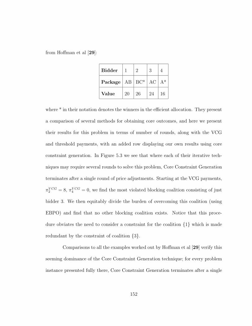
from Hoffman et al [29]:
Bidder 1 2 3 4
Package AB BC* AC A*
Value 20 26 24 16
where * in their notation denotes the winners in the efficient allocation. They present
a comparison of several methods for obtaining core outcomes, and here we present
their results for this problem in terms of number of rounds, along with the VCG
and threshold payments, with an added row displaying our own results using core
constraint generation. In Figure 5.3 we see that where each of their iterative tech-
niques may require several rounds to solve this problem, Core Constraint Generation
terminates after a single round of price adjustments. Starting at the VCG payments,
πV CG2 = 8, πV CG
4 = 0, we find the most violated blocking coalition consisting of just
bidder 3. We then equitably divide the burden of overcoming this coalition (using
EBPO) and find that no other blocking coalition exists. Notice that this proce-
dure obviates the need to consider a constraint for the coalition {1} which is made
redundant by the constraint of coalition {3}.
Comparisons to all the examples worked out by Hoffman et al [29] verify this
seeming dominance of the Core Constraint Generation technique; for every problem
instance presented fully there, Core Constraint Generation terminates after a single
152
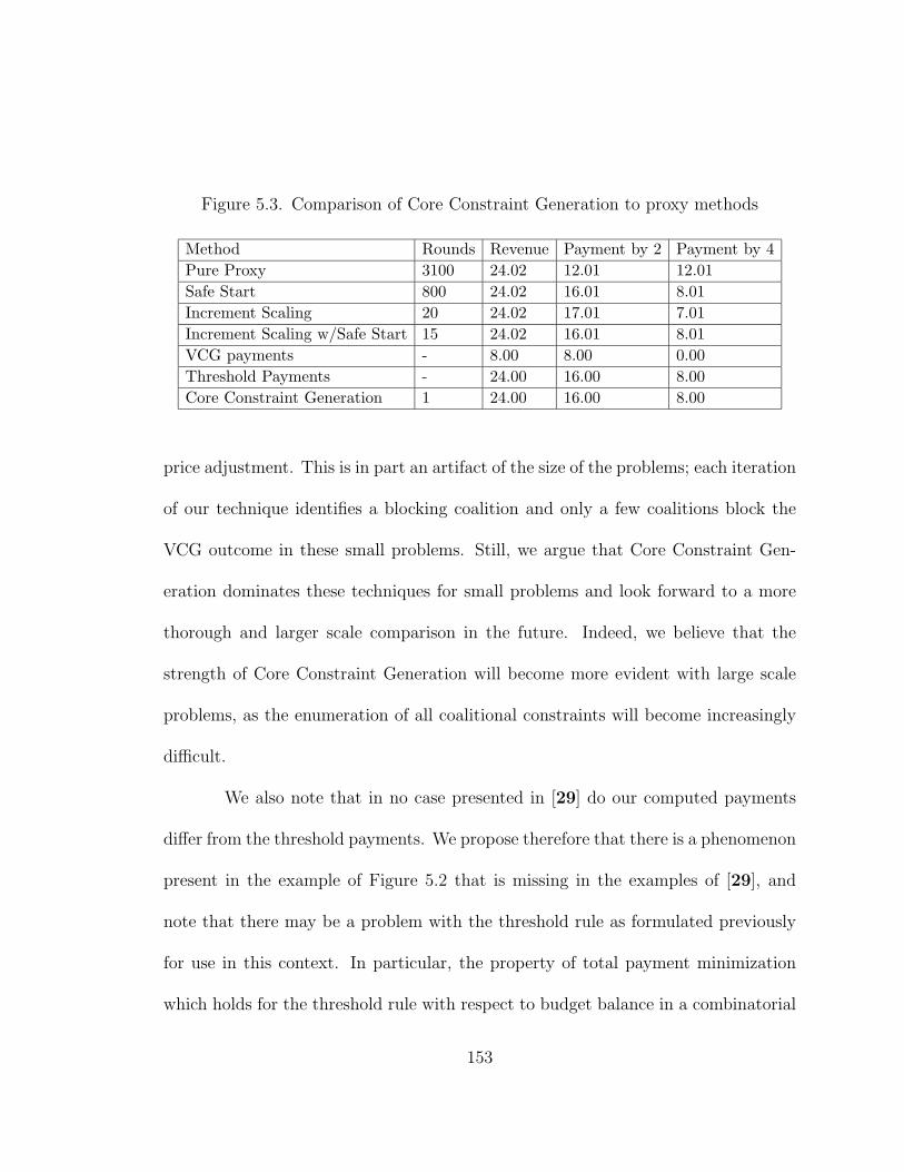
Figure 5.3. Comparison of Core Constraint Generation to proxy methods
Method Rounds Revenue Payment by 2 Payment by 4
Pure Proxy 3100 24.02 12.01 12.01
Safe Start 800 24.02 16.01 8.01
Increment Scaling 20 24.02 17.01 7.01
Increment Scaling w/Safe Start 15 24.02 16.01 8.01
VCG payments - 8.00 8.00 0.00
Threshold Payments - 24.00 16.00 8.00
Core Constraint Generation 1 24.00 16.00 8.00
price adjustment. This is in part an artifact of the size of the problems; each iteration
of our technique identifies a blocking coalition and only a few coalitions block the
VCG outcome in these small problems. Still, we argue that Core Constraint Gen-
eration dominates these techniques for small problems and look forward to a more
thorough and larger scale comparison in the future. Indeed, we believe that the
strength of Core Constraint Generation will become more evident with large scale
problems, as the enumeration of all coalitional constraints will become increasingly
difficult.
We also note that in no case presented in [29] do our computed payments
differ from the threshold payments. We propose therefore that there is a phenomenon
present in the example of Figure 5.2 that is missing in the examples of [29], and
note that there may be a problem with the threshold rule as formulated previously
for use in this context. In particular, the property of total payment minimization
which holds for the threshold rule with respect to budget balance in a combinatorial
153
exchange (as in Parkes, Kalagnanam, and Eso [56]) does not hold for the threshold
rule with respect to core constraints in a one-sided auction (as formulated in Parkes
[54] and Hoffman et al [29]). Since our EBPO payment rule and the threshold rule
share the same intention, it appears that the example of Figure 5.2 illustrates a
previously unnoticed property of the threshold rule, and suggest that a refinement
of its formulation in which total payments are minimized explicitly is needed in the
context of one-sided auctions and core constraints.
5.3. Remarks on Core Constraint Generation
The example of Figure 5.2 helps to justify our proposal that total payment
minimization within the core should be the “primary” objective of payment deter-
mination with payment equity following as a “secondary” objective, used only to
distinguish between multiple optima. Perceived fairness may be an even stronger
motivation to adopt such a payment rule. For governmental auctions in particular,
many will take comfort that the auctioneer is not selecting an outcome according
to self interest, but in the combined best interests of the bidders. In private sector
B2B auctions, on the other hand, assurance of an auction that reaps benefits in a
minimal fashion may be the best method to maintain long-term trade relationships
and encourage repeated participation. Only the core constraints, representing com-
petition, should drive up the payments, not the artificial device used to determine
payments.
154
Additionally, we feel that our method offers computational benefits over
other techniques described in the recent literature. By solving the separation prob-
lem at each point in payment space we only consider coalitions that actually threaten
to block a potential outcome, obviating the need to apply the entire exponential set
of constraints. We feel that the formulation of the separation problem for violated
core constraints and the development of a price adjustment procedure utilizing this
approach are novel contributions to the literature. This separation paradigm has
proven useful elsewhere for the solution of optimization problems with an exponen-
tial number of constraints (e.g. traveling salesman problems), and we hope that
forthcoming experiments will verify this for Core Constraint Generation.
Further, our price adjustment procedure takes place without the need for
a price increment as in the ascending proxy technique, accelerated or otherwise.
EBPOt upholds every generated core constraint for the remainder of the procedure.
This ensures that the same coalition will not appear repeatedly as blocking in our
procedure. Experience with the ascending proxy method, on the other hand, shows
that after an increment and re-solution of the winner determination problem, the
same coalition may appear for several iterations. Instead, our method finds the
interesting “change points” implicitly and prescribes adequate payment adjustments
at each iteration, rather than requiring the guess of an appropriate increment as a
parameter.
155

As a final note on our comparison to ascending proxy techniques, we do rec-
ognize that our method has inferior privacy-preservation properties to the ascending
proxy auction as presented by Ausubel and Milgrom [5]. Their method can be im-
plemented such that demand is only revealed incrementally to the auctioneer, while
our method requires the auctioneer to “open up the proxy” and use all information
submitted by the bidders to determine the outcome. We are motivated, however,
by Hoffman et al [29], who show that the ascending proxy auction can be acceler-
ated by opening up the proxy for use in winner determination. As their research
suggests, if it is possible to trust a third party to securely determine the auction
outcome without unnecessary public knowledge of the bid submission, then access
to all bid information can lead to a more rapid conclusion of a sealed-bid combina-
torial auction. We hope that future computational studies will confirm that Core
Constraint Generation can accelerate the determination of a bidder-Pareto-optimal
core outcome in a sealed-bid auction.
156

CHAPTER 6
Matrix Bidding
In Chapter 3, we revealed that because of the gross substitutes property bid
tables cannot express preferences for complementary bundles, a potential weakness.
In Chapter 4, we showed how a more complete set of preferences could be supported
in an auction with multiple stages used to reveal the different types of preferences
which could not be achieved in a bid table. In this chapter, we explore an alternative
method for expressing mixed (both positive and negative) synergy, while still utilizing
the compactness provided by a price-vector agent format. We accomplish this by
imposing a form of ranked cooperation among the price-vector agents and find that
we are rewarded with a wide array of possible preference expression in a compact
format that we call Matrix Bidding.
We begin this chapter with the basics of matrix bids and motivate how they
can be used with a few examples. In §6.2, we provide an IP formulation of the winner
determination problem for a Matrix Bid Auction (MBA) and show that in general
this problem is NP-hard. In §6.3 we provide a deeper exploration of the preference
expression afforded by the matrix bid format and compare the logical language of
matrix bids to other logical languages from the literature.
157
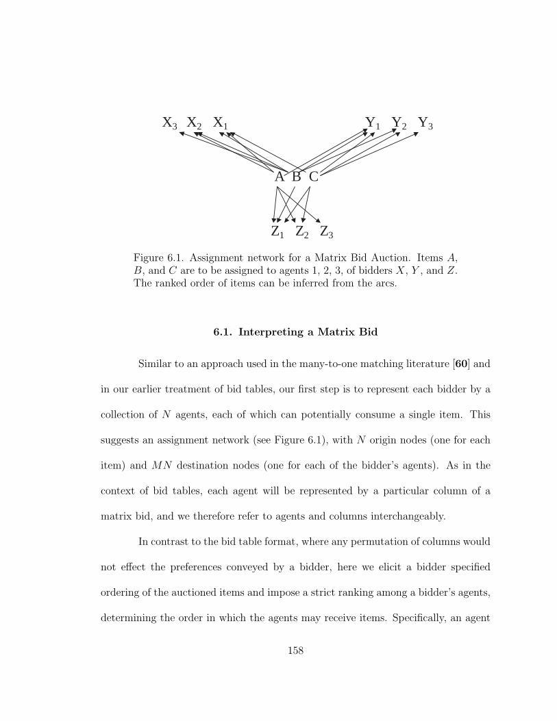
A B C
X3 X2 X1 Y1 Y2 Y3
Z1 Z2 Z3
Figure 6.1. Assignment network for a Matrix Bid Auction. Items A,B, and C are to be assigned to agents 1, 2, 3, of bidders X, Y , and Z.The ranked order of items can be inferred from the arcs.
6.1. Interpreting a Matrix Bid
Similar to an approach used in the many-to-one matching literature [60] and
in our earlier treatment of bid tables, our first step is to represent each bidder by a
collection of N agents, each of which can potentially consume a single item. This
suggests an assignment network (see Figure 6.1), with N origin nodes (one for each
item) and MN destination nodes (one for each of the bidder’s agents). As in the
context of bid tables, each agent will be represented by a particular column of a
matrix bid, and we therefore refer to agents and columns interchangeably.
In contrast to the bid table format, where any permutation of columns would
not effect the preferences conveyed by a bidder, here we elicit a bidder specified
ordering of the auctioned items and impose a strict ranking among a bidder’s agents,
determining the order in which the agents may receive items. Specifically, an agent
158
may not receive an item unless the next higher ranked agent receives a higher ranked
item.
To define the relationship between items and agents more precisely, we say
that each bidder j in this format must submit a numerical ranking rij for each of the
N items at auction. We say that rij = 1 if item i is the first (highest ranked) item
in bidder j’s ordering of the items, rij = 2 if item i is the second item in bidder j’s
ordering, etc. We require that this ranking be strict and total for each bidder j: if
i1 6= i2, then ri1j 6= ri2j, and ∀n ≤ N , ∃i ∈ I with rij = n. It is important to note that
the rankings specified by the values of rij are intended only to guide the coordination
of the ranked agents and do not necessarily reflect any preference ordering among
the items for that bidder. Stated differently ri1j < ri2j ; vj({i1}) ≥ vj({i2}).
For each of bidder j’s agents (j, k), define the binary acceptance variable
xijk = 1 if agent (j, k) receives item i, and xijk = 0 otherwise. With this terminology
defined, we may now state the cooperation restriction among a particular bidder’s
agents:
∀k > 1, xijk = 1 ⇒ xıjk−1 = 1 for some ı with rıj < rij
This says that any agent (other than agent 1) may not receive an item unless the
next more highly ranked agent receives a more highly ranked item. The preference
restriction imposed in the matrix bid auction is that the value an item brings to a
bidder is determined only by its ranking relative to the other items in the bundle
159

(i.e. which agent it is assigned to). Although this may at first seem restrictive, we
will show that when used effectively a great deal can be said by each bidder.
A bidder in this model specifies her preferences with a value for each item in
each of its possible rankings in the final bundle. The bid offered for item i by bidder
j given that it is the kth best item she receives will be denoted bijk. Bidder j’s bid
on a bundle S may then be computed as:
bj(S) =∑
i∈S
bijk(i,S)
where k(i, S) gives the ordinal ranking of item i among the items in S. For example,
k(ı, S) = 1 if no item in S has a higher rank (smaller value of rij) than item ı.
Similarly, k(ı, S) = 2 if exactly one item has a higher rank than item ı, etc.
Each bidder submits an ordered list of the items to establish the values of
rij and a matrix containing non-negative values of bijk (without loss of generality
we assume integer values throughout). The matrix of bijk entries together with the
precedence ordering rij is referred to as a matrix bid. In each matrix bid a row will
be associated with a particular item, and each column will be associated with an
agent. The item associated with a given row is written to the left of that row, with
the row of the highest ranked item on top, the second highest item beneath it etc.
Since the kth item in the ordering can be at most the kth item in any bundle, the
matrix of bijk values will be lower triangular.
160
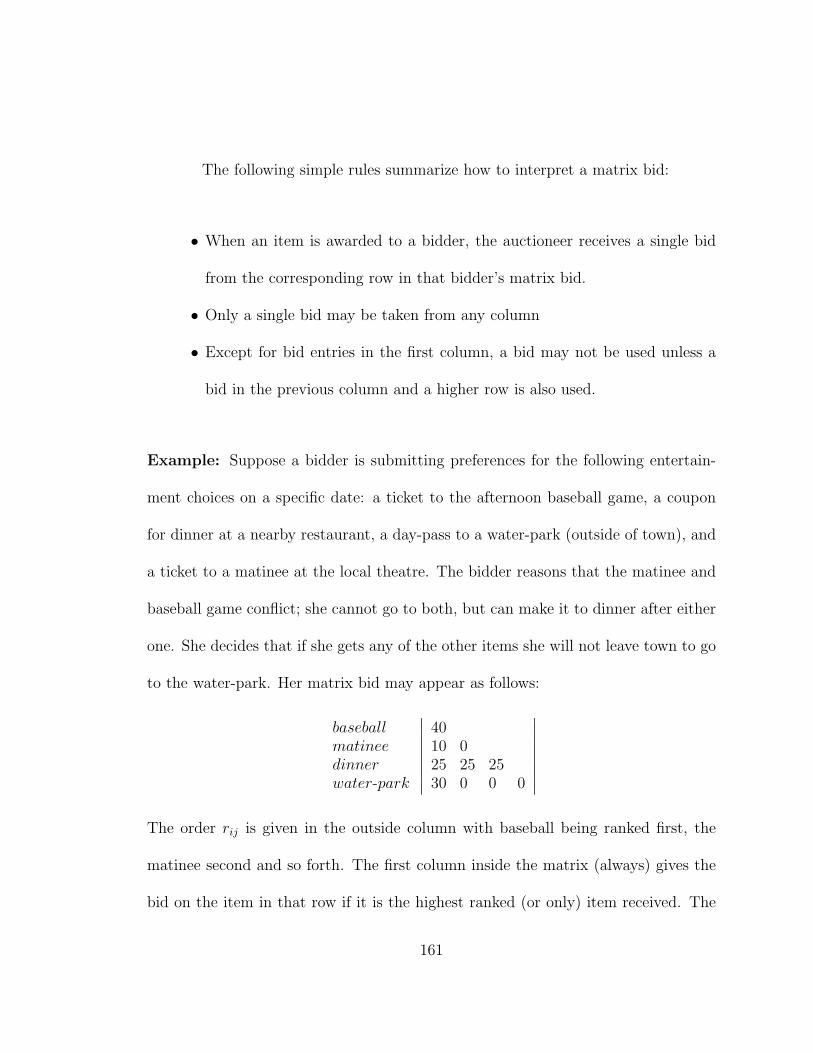
The following simple rules summarize how to interpret a matrix bid:
• When an item is awarded to a bidder, the auctioneer receives a single bid
from the corresponding row in that bidder’s matrix bid.
• Only a single bid may be taken from any column
• Except for bid entries in the first column, a bid may not be used unless a
bid in the previous column and a higher row is also used.
Example: Suppose a bidder is submitting preferences for the following entertain-
ment choices on a specific date: a ticket to the afternoon baseball game, a coupon
for dinner at a nearby restaurant, a day-pass to a water-park (outside of town), and
a ticket to a matinee at the local theatre. The bidder reasons that the matinee and
baseball game conflict; she cannot go to both, but can make it to dinner after either
one. She decides that if she gets any of the other items she will not leave town to go
to the water-park. Her matrix bid may appear as follows:
baseballmatineedinnerwater-park
∣
∣
∣
∣
∣
∣
∣
∣
4010 025 25 2530 0 0 0
∣
∣
∣
∣
∣
∣
∣
∣
The order rij is given in the outside column with baseball being ranked first, the
matinee second and so forth. The first column inside the matrix (always) gives the
bid on the item in that row if it is the highest ranked (or only) item received. The
161
second column gives the price for each item in the row given that it is the second
highest item received etc.
If she receives a baseball ticket she is willing to pay 0 for the matinee which
she cannot attend due to conflict. If she receives either baseball or matinee in the
first column she would being willing to pay 25 for the meal (in the second column).
Although the seller is unlikely to give away the matinee ticket, the mathematical
formulation does not necessarily rule this out. If the auctioneer gives her the baseball
ticket at 40 and the matinee ticket at 0, she is still willing to pay 25 for the dinner,
and expresses this with a 25 in the third column; a free matinee ticket does not
change her preferences for the dinner. The fourth row shows that she would pay 30
for the water-park pass by itself, but would pay 0 for it if any other items are won.
The bid of 30 cannot be accepted with any other bid by the rules outlined above.
Example: A major television network is hosting a worldwide television event with
a limited number of available advertising time-slots; for simplicity we assume there
are four time-slots, A, B, C, and D, chronologically. They attract companies X, Y ,
and Z who have very different marketing strategies determining their preferences for
these time-slots.
BidderX has developed a two-part “gag” commercial which they will only
use if they can secure exactly two time-slots. They are indifferent to which two.
162
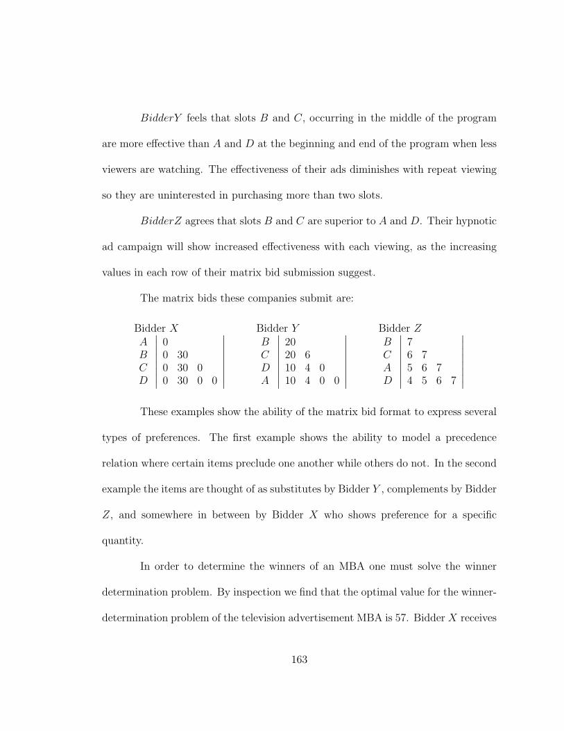
BidderY feels that slots B and C, occurring in the middle of the program
are more effective than A and D at the beginning and end of the program when less
viewers are watching. The effectiveness of their ads diminishes with repeat viewing
so they are uninterested in purchasing more than two slots.
BidderZ agrees that slots B and C are superior to A and D. Their hypnotic
ad campaign will show increased effectiveness with each viewing, as the increasing
values in each row of their matrix bid submission suggest.
The matrix bids these companies submit are:
Bidder XABCD
∣
∣
∣
∣
∣
∣
∣
∣
00 300 30 00 30 0 0
∣
∣
∣
∣
∣
∣
∣
∣
Bidder YBCDA
∣
∣
∣
∣
∣
∣
∣
∣
2020 610 4 010 4 0 0
∣
∣
∣
∣
∣
∣
∣
∣
Bidder ZBCAD
∣
∣
∣
∣
∣
∣
∣
∣
76 75 6 74 5 6 7
∣
∣
∣
∣
∣
∣
∣
∣
These examples show the ability of the matrix bid format to express several
types of preferences. The first example shows the ability to model a precedence
relation where certain items preclude one another while others do not. In the second
example the items are thought of as substitutes by Bidder Y , complements by Bidder
Z, and somewhere in between by Bidder X who shows preference for a specific
quantity.
In order to determine the winners of an MBA one must solve the winner
determination problem. By inspection we find that the optimal value for the winner-
determination problem of the television advertisement MBA is 57. Bidder X receives
163
items A and D, contributing 30 to the objective function; Bidder Y receives item C
for 20 units, while Bidder Z pays 7 units for B. In the next section we present an
integer programming formulation for finding the winners in an MBA.
6.2. Integer Programming Formulation of Winner Determination
The winner-determination problem, in this context, is to find the maximum
revenue assignment of items to agents, satisfying supply of one for each item and
demand of at most one for each agent, as well as upholding the ordering or ranking of
items. According to the ranking, a feasible assignment may assign an item to a given
agent only if the agents for a particular bidder with a lower value of k are assigned
items with a lower value of rij. These constraints are formalized in the following IP
which we will refer to as MBA:
164
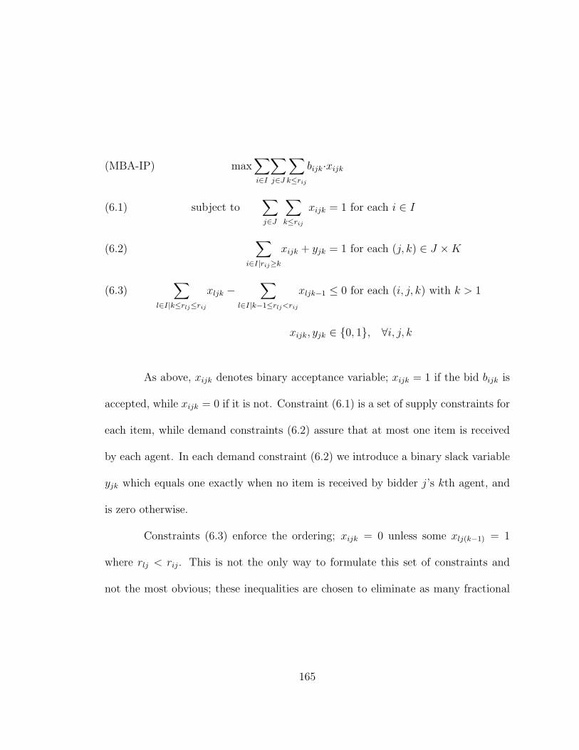
max∑
i∈I
∑
j∈J
∑
k≤rij
bijk·xijk(MBA-IP)
subject to∑
j∈J
∑
k≤rij
xijk = 1 for each i ∈ I(6.1)
∑
i∈I|rij≥k
xijk + yjk = 1 for each (j, k) ∈ J × K(6.2)
∑
l∈I|k≤rlj≤rij
xljk −∑
l∈I|k−1≤rlj<rij
xljk−1 ≤ 0 for each (i, j, k) with k > 1(6.3)
xijk, yjk ∈ {0, 1}, ∀i, j, k
As above, xijk denotes binary acceptance variable; xijk = 1 if the bid bijk is
accepted, while xijk = 0 if it is not. Constraint (6.1) is a set of supply constraints for
each item, while demand constraints (6.2) assure that at most one item is received
by each agent. In each demand constraint (6.2) we introduce a binary slack variable
yjk which equals one exactly when no item is received by bidder j’s kth agent, and
is zero otherwise.
Constraints (6.3) enforce the ordering; xijk = 0 unless some xlj(k−1) = 1
where rlj < rij. This is not the only way to formulate this set of constraints and
not the most obvious; these inequalities are chosen to eliminate as many fractional
165
solutions as possible while enforcing the ordering by including more than is nec-
essary in the first summation. Padberg and Alevras [52] study the “order pre-
serving assignment problem” which corresponds exactly to an instance of MBA-IP
with only a single bidder, and potentially less than N agents. They show for their
own formulation that the ordering may be enforced with constraints like those of
(6.3), and in particular that constraints in this form are facet defining. To see that
this formulation of the ordering constraints is superior to the “natural” version (i.e.
xijk −∑
l∈I|k−1≤rlj<rij
xljk−1 ≤ 0 for each (i, j, k) with k > 1) observe that in a three
item auction for items A, B, and C with rA1 = 1, rB1 = 2, and rC1 = 3 it is possi-
ble to have a fractional solution with xA11 = xB12 = xC12 = 12
using the “natural”
constraints while the constraints (6.3) do not admit such a solution.
Although the assignment problem is polynomially solvable, adding con-
straints (6.3) greatly complicates the matter. In particular, it is not hard to find
examples in which the LP-relaxation of MBA-IP will produce a fractional optimal
solution. Interestingly, Padberg and Alevras [52] show that the order preserving
assignment problem is polynomially solvable (Lemma 6.2 below generalizes their re-
sult), while Theorem 6.1 shows that the winner determination problem for an MBA
is NP-hard. In other words evaluating one’s own matrix bid can be done in polyno-
mial time, while finding an assignment that simultaneously satisfies several orderings
(one for each matrix bid) represents a hard decision problem for the auctioneer.
166
We now verify one strength of the formulation MBA-IP: it is polynomially-
sized in the number of items and bidders, unlike the general winner determination
problem (GWD) which requires an exponential number of variables, one for every
bidder/bundle pair. This suggests that for some values of N a GWD auction cannot
be performed due to memory restrictions, while an MBA may still be held for the
same set of N items. To verify this, we note that each bidder must submit each
matrix bid entry or 1+2+3+ ...N different bids due to the triangular shape of each
bid matrix. Each bidder thus submits∑N
l=1 l = N(N+1)2
bid entries and an ordered
list of N items, 12N2 + 3
2N pieces of information. The total number of x variables is
equal to the total number of matrix bid entries M · N(N+1)2
, while the total number
of y variables is simply MN . Counting the constraints similarly according to their
indices we find that there are N of type (6.1), MN of type (6.2), and M · N(N−1)2
of
type (6.3). Thus, MBA-IP has 12N2M + 3
2NM variables and 1
2N2M + 1
2NM + N
constraints. Our computational results (Chapter 7) suggest that for reasonable N
and M , MBA-IP instances of this size can be solved quickly enough for auction
implementation purposes, despite the following theorem.
Theorem 6.1. The winner determination problem for a matrix bid auction is NP-
hard.
Proof. We employ the NP-hard Weighted Set-Packing Problem (WSP): Given a set
S, and a list of subsets of S: S1, S2, ... Sp, each with a corresponding weight w1, w2,
167

... wp, problem WSP asks for the maximum weight collection of mutually-disjoint
Sis.
The transformation of this general instance of WSP into a matrix bid auction
proceeds in a straightforward manner. Identify S from the WSP with I and create
p bidders, one for each Si. Each (single-minded) bidder will submit a matrix bid
with the elements of this particular Si shuffled to the top of the matrix ordering,
and a bid of wp placed in the |Si|th diagonal entry. An optimal solution to the
winner-determination problem for this auction MBA-IP provides a maximum weight
set-packing of S1, S2, ... Sp. �
Despite this classification of the decision problem as NP-hard, our experi-
ence tells us that the formulation MBA-IP is fairly well-behaved. It is well known
that the assignment constraints (6.1) and (6.2) on their own define a feasible region
with integer extreme points. With the addition of constraints (6.3) many of these
extreme points are removed and several fractional extreme points are introduced to
the polyhedron. Exactly how many of each type are generated or eliminated by (6.3)
varies among instances (even of the same size) depending on the orderings chosen by
bidders. Every integer solution to MBA-IP, however, is also a feasible assignment
and thus an extreme point of the region defined without (6.3), partially explaining
the proliferation of LP-relaxation solutions that are integer optimal as seen in our
experiments. Another partial explanation is suggested by the following lemma.
168
Lemma 6.2. For any bidder j, if∑
k xijk ∈ {0, 1} for all items i ∈ I, then xijk ∈
{0, 1} for all i and k.
Proof. The implication is trivial for all i such that∑
k xijk = 0, so we consider the
case in which∑
k xijk = 1.
Let i1 = arg minIj
rij, where Ij = {i|∑
k xijk = 1} (i.e. Ij is the set of all
items awarded to j). Similarly, let i2 = arg minIj\{i1}
rij, i3 = arg minIj\{i1,i2}
and so forth,
yielding in general that in is the nth ranked item in Ij.
First note that since there is no item l with rlj < ri1j and xljk 6= 0, constraints
(6.3) for i1 imply that xi1jk ≤ 0 for all k > 1, and therefore xi1jk = 0 for all k > 1.
Since∑
k xi1jk = 1, it must be the case that xi1j1 = 1. By (6.2) it also follows that
xij1 = 0 for all i 6= i1.
Next, we claim that if xinjn = 1 for all n < k, then xikjk = 1. This is easily
shown since xinjn = 1 for all n < k implies that:
xijk = 0 for all k ≥ k and i with rij < rikj(6.4)
xikjk = 0 for all k < k(6.5)
The first of these two facts (6.4), together with (6.3), implies that xikjk = 0 for all
k > k. Using this with (6.5) and∑
k xikjk = 1 we obtain the desired result, xi
kjk = 1.
The lemma now follows by induction. �
169

Lemma 6.2 states roughly that if a bidder j receives integer amounts of all
items (among all her agents), the constraints of MBA-IP dictate that the assignment
of items to bidder j’s collection of agents must be integral. Alternatively, items may
not be split fractionally among the agents of a single bidder j, unless there is some
item which j shares fractionally with a different bidder.
The polynomial-solvability of the order-preserving assignment, first proved
by Padberg and Alevras [52], follows as a special case of Lemma 6.2, which implies
that the polyhedron defined by constraints (6.1), (6.2), and (6.3) with just a single
bidder has integer extreme points. Further, Lemma 6.2 offers an alternate and more
succinct proof than Padberg and Alevras [52].
As stated here, Lemma 6.2 suggests the possibility of an advantageous
branching strategy when using a branch-and-bound technique to solve MBA-IP.
Rather than branching on a single variable at each node in the branch-and-bound
tree, it seems possible to benefit by branching on a bidder/item pair, dictating that
the specific item definitely be awarded to bidder j on one branch, and that the item
definitely not be awarded to bidder j on the other branch. It is advantageous to
focus on bidder/item pairs corresponding to items split fractionally among several
bidders, since by Lemma 6.2, if these bidder/item pairs don’t exist, then items will
not be split fractionally among the agents of the same bidder, and the resulting
solution must therefore be integer.
170

How to choose such a bidder/item pair to branch on when many candidates
are available is itself a difficult question. Indeed, so far in our computational exper-
iments, a robust heuristic for this MBA subproblem has remained elusive. Several
versions of a specialized branching strategy have been investigated as part of our
research, though none is able to challenge CPLEX 8.0’s default branching algorithm
(which itself applies several heuristics for faster branching). We believe that the
pursuit of a branching strategy based on this observation remains worthy of future
study.
6.3. Preference Expression using Matrix Bids
In this section we explore how matrix bids may be used to convey preferences.
We suggest the use of matrix bids as “atomic bids” to be combined with the logical
connectives, offering a new notational system for writing down preferences that are
difficult to express with flat bids alone. We show that a language with matrix bids
as atoms is more expressive in a polynomial amount of input than a language with
just flat bids as atoms, and equally as expressive as a flat-bid language augmented
with “k-of” or “exactly-k-of” bids.
Relative to other logical bidding languages we show that more can be said
with a single atom, and that some things can be said easily in matrix bids that
are cumbersome in other languages. On the whole we hope to convey that with
some experience matrix bids may be an easier to read format than the equivalent
171
collection of bids needed express the same preferences in a language with “k-of” and
“exactly-k-of” operators applied to flat bids only. Matrix bids provide a structured
way to string together several “k-of”, “exactly-k-of”, and flat bid sentence fragments
to be read in a meaningful way after deleting many of the logical connectives. In
§7.2, we will see that this allows us to quickly generate simulated auction data (with
no logical connectives) which would have required exponentially long bid sentences
in any of the flat-bid auction simulations commonly found in recent literature (e.g.
[28], [41] ,[65]).
As first discussed in Chapter 2, let a flat bid be denoted (S, p), for an all-
or-nothing bid of p monetary units on the set of items S. As noted by Nisan [50],
certain natural expressions of preference can require exponentially long bid sentences
in a logical language with only flat bids as atoms. The work of Boutillier and Hoos
([9], [10], [30]) explore the possibility of expanding the bid language to include a
“k-of” operator, handling one of the most natural expressions that are tiresome to
convey in flat bids by simply adding it in explicitly. At first, this does not seem
that rewarding in terms of the impact on winner determination, because the authors
simply expand a k-of expression back into flat bids prior to winner determination.
But Boutillier [9] later shows how to explicitly model the k-of operator in an IP
formulation of winner determination with a new class of constraints to handle the
new operator.
172
In this same spirit we ask: are their other natural preference types that are
difficult to handle in a logical language of flat bids? Should the list of connectives be
augmented to accept other forms of preferences like the k-of operator? One example
of another natural connective is the “exactly k-of” operator, where the k-of opera-
tor discussed elsewhere could be called more precisely the “at least k-of” operator
(though we will continue to refer to this one as the k-of operator). It is not difficult
to show that the exactly k-of operator can be handled in an IP winner determination
formulation with specialized constraints as the k-of operator is handled in [9].
Adding more and more basic connectives and new classes of constraints seem
to complicate the matter. Reading and writing bids in such a language becomes diffi-
cult (for a human user) with many connectives and complicated nestings to consider
when putting together an entire bid sentence or a complete profile of preferences. Is
there instead an atomic format which can accept a wide variety of preferences includ-
ing in particular those that are difficult to express in flat-bids alone? We propose
that matrix bids offer such a format and that a logical language of matrix bids can
be made at least as expressive in a polynomial amount of input space as any of the
other languages in the literature. This latter statement is justified by comparison
to the language LGB of [9], which in turn is at least as expressive as any language
that precedes it. In particular, if we let Lflat be the language LGB of [9] without the
k-of operator, and LMB be the language formed with matrix bids as atoms and the
173

same logical connectives as in LGB, we will show that the preferences which can be
expressed compactly in Lflat are properly contained in LMB, while the preferences
which can be expressed compactly in LMB are exactly equal to the preferences which
can be expressed compactly in LGB.
6.3.1. Capacity Constraints and Capacity Costs
We begin with an illustrative demonstration of one of the strengths of matrix
bids relative to the language Lflat, which is composed of flat bids joined by the
logical connectives AND, OR, and XOR. We show how simple capacity-constraints
are naturally expressed in a matrix bid, and compare with the equivalent formulation
in Lflat.
Suppose we have an auction with N = 6 and a bidder wants to express an
additive valuation over the items with a constraint that he cannot consume more
than 3 items. A matrix bid expressing this (with arbitrary values given for each
item) is as follows:ABCDEF
∣
∣
∣
∣
∣
∣
∣
∣
∣
∣
∣
2218 1817 17 1716 16 16 014 14 14 0 012 12 12 0 0 0
∣
∣
∣
∣
∣
∣
∣
∣
∣
∣
∣
With this bid, he pays the same cost for each item regardless of what other items he
gets, but will never pay a positive amount for a fourth, fifth, or sixth item, reflected
by the zeros in the fourth, fifth, and sixth columns. For a comparison of size and
174
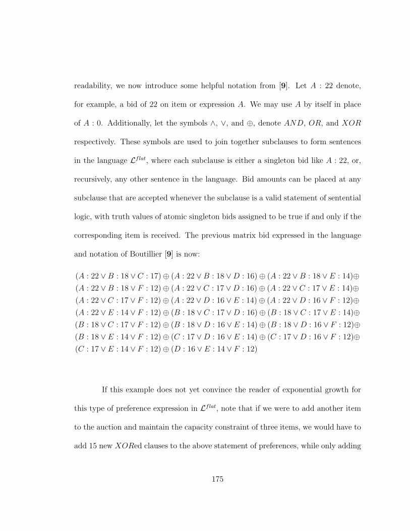
readability, we now introduce some helpful notation from [9]. Let A : 22 denote,
for example, a bid of 22 on item or expression A. We may use A by itself in place
of A : 0. Additionally, let the symbols ∧, ∨, and ⊕, denote AND, OR, and XOR
respectively. These symbols are used to join together subclauses to form sentences
in the language Lflat, where each subclause is either a singleton bid like A : 22, or,
recursively, any other sentence in the language. Bid amounts can be placed at any
subclause that are accepted whenever the subclause is a valid statement of sentential
logic, with truth values of atomic singleton bids assigned to be true if and only if the
corresponding item is received. The previous matrix bid expressed in the language
and notation of Boutillier [9] is now:
(A : 22 ∨ B : 18 ∨ C : 17) ⊕ (A : 22 ∨ B : 18 ∨ D : 16) ⊕ (A : 22 ∨ B : 18 ∨ E : 14)⊕
(A : 22 ∨ B : 18 ∨ F : 12) ⊕ (A : 22 ∨ C : 17 ∨ D : 16) ⊕ (A : 22 ∨ C : 17 ∨ E : 14)⊕
(A : 22 ∨ C : 17 ∨ F : 12) ⊕ (A : 22 ∨ D : 16 ∨ E : 14) ⊕ (A : 22 ∨ D : 16 ∨ F : 12)⊕
(A : 22 ∨ E : 14 ∨ F : 12) ⊕ (B : 18 ∨ C : 17 ∨ D : 16) ⊕ (B : 18 ∨ C : 17 ∨ E : 14)⊕
(B : 18 ∨ C : 17 ∨ F : 12) ⊕ (B : 18 ∨ D : 16 ∨ E : 14) ⊕ (B : 18 ∨ D : 16 ∨ F : 12)⊕
(B : 18 ∨ E : 14 ∨ F : 12) ⊕ (C : 17 ∨ D : 16 ∨ E : 14) ⊕ (C : 17 ∨ D : 16 ∨ F : 12)⊕
(C : 17 ∨ E : 14 ∨ F : 12) ⊕ (D : 16 ∨ E : 14 ∨ F : 12)
If this example does not yet convince the reader of exponential growth for
this type of preference expression in Lflat, note that if we were to add another item
to the auction and maintain the capacity constraint of three items, we would have to
add 15 new XORed clauses to the above statement of preferences, while only adding
175

7 new numbers (one new row) to the matrix bid. In general, additive preferences for
n items with a capacity constraint of k takes (nk) clauses, each containing k atomic
bids in the language of Lflat, or a single matrix bid of size (n2 ) = n(n−1)
2, verifying
that LMB can contain preferences in a single matrix bid that require a sentence of
exponential length in Lflat.
This example demonstrates how to apply a capacity constraint using a ma-
trix bid and is not limited to a situation where the underlying preferences are ad-
ditive. Though we used an additive structure in this example for simplicity, one
could start within any matrix bid expression and “zero out” columns that exceed
capacity. Further, matrix bids easily handle a capacity cost structure in place of a
hard capacity constraint. Imagine a firm that experiences an underlying additive
structure (again for simplicity) for items received (for example, in terms of potential
revenue generated), but then wishes to capture storage and maintenance costs based
on the number of items in their possession.
Suppose, for example, that in a 6 item auction they experience storage and
maintenance costs of 0 for the first two items, but have to employ a new worker (at
a cost of 3 units) to maintain every two items they purchase after that, and further
must rent a storage area at 1 unit each for the fifth and sixth items. If their additive
176

revenue structure is captured in the following matrix bid:
ABCDEF
∣
∣
∣
∣
∣
∣
∣
∣
∣
∣
∣
2218 1817 17 1716 16 16 1614 14 14 14 1412 12 12 12 12 12
∣
∣
∣
∣
∣
∣
∣
∣
∣
∣
∣
then they can subtract the entries of the following row vector from each entry in the
corresponding column to capture the storage and maintenance costs:
0 0 3 0 4 1
Thus if revenue accrues additively with the values from the above matrix bid, and
costs are as described above, the preferences of this firm are captured in the following
matrix bid:ABCDEF
∣
∣
∣
∣
∣
∣
∣
∣
∣
∣
∣
2218 1817 17 1416 16 13 1614 14 11 14 1012 12 9 12 8 11
∣
∣
∣
∣
∣
∣
∣
∣
∣
∣
∣
Now, they have compactly submitted a bid with positive value for each of the 2N −1
possible non-empty bundles, while Lflat cannot express the generalized version of
these preferences compactly. To be certain, note that the information conveyed in
the first three columns requires as much space in a Lflat sentence as in the previous
example, and that both examples easily generalize due to the underlying additive
preference structure.
177
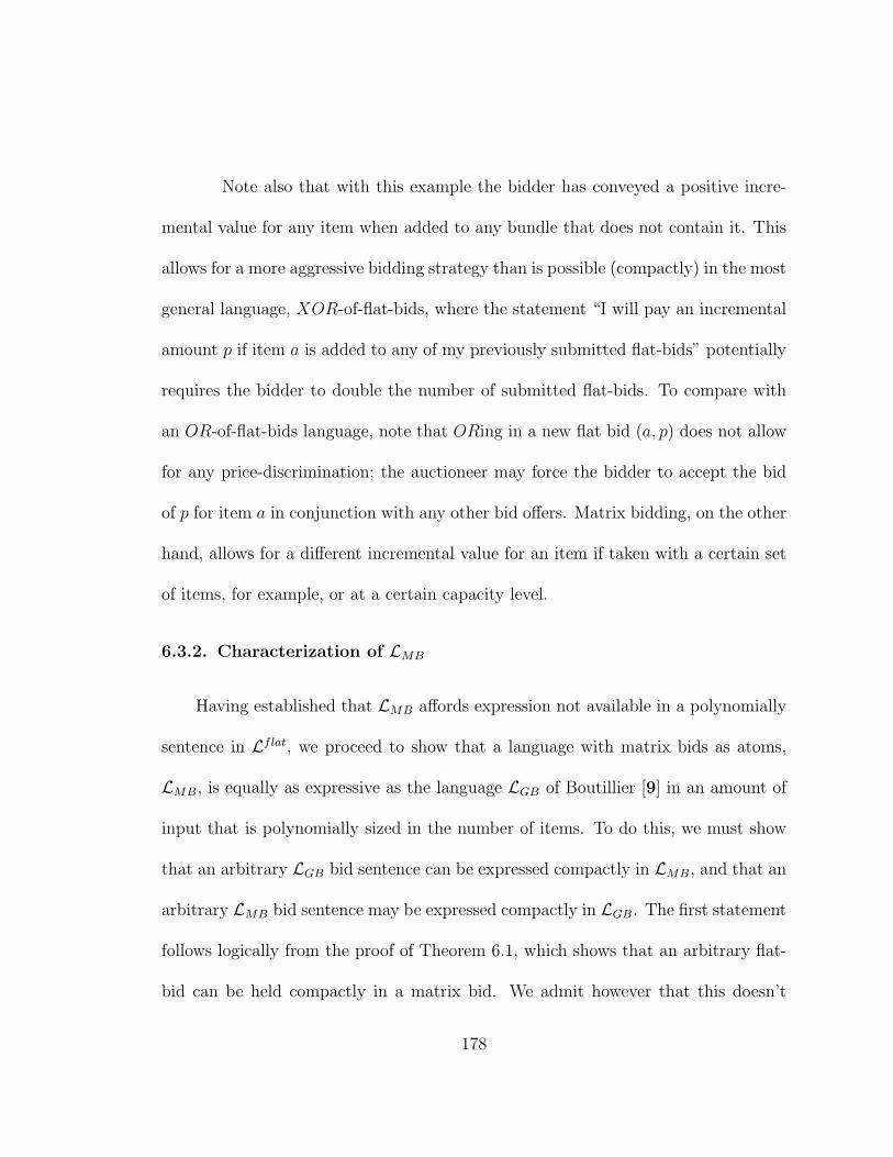
Note also that with this example the bidder has conveyed a positive incre-
mental value for any item when added to any bundle that does not contain it. This
allows for a more aggressive bidding strategy than is possible (compactly) in the most
general language, XOR-of-flat-bids, where the statement “I will pay an incremental
amount p if item a is added to any of my previously submitted flat-bids” potentially
requires the bidder to double the number of submitted flat-bids. To compare with
an OR-of-flat-bids language, note that ORing in a new flat bid (a, p) does not allow
for any price-discrimination; the auctioneer may force the bidder to accept the bid
of p for item a in conjunction with any other bid offers. Matrix bidding, on the other
hand, allows for a different incremental value for an item if taken with a certain set
of items, for example, or at a certain capacity level.
6.3.2. Characterization of LMB
Having established that LMB affords expression not available in a polynomially
sentence in Lflat, we proceed to show that a language with matrix bids as atoms,
LMB, is equally as expressive as the language LGB of Boutillier [9] in an amount of
input that is polynomially sized in the number of items. To do this, we must show
that an arbitrary LGB bid sentence can be expressed compactly in LMB, and that an
arbitrary LMB bid sentence may be expressed compactly in LGB. The first statement
follows logically from the proof of Theorem 6.1, which shows that an arbitrary flat-
bid can be held compactly in a matrix bid. We admit however that this doesn’t
178
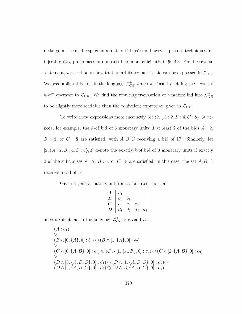
make good use of the space in a matrix bid. We do, however, present techniques for
injecting LGB preferences into matrix bids more efficiently in §6.3.3. For the reverse
statement, we need only show that an arbitrary matrix bid can be expressed in LGB.
We accomplish this first in the language L+GB which we form by adding the “exactly
k-of” operator to LGB. We find the resulting translation of a matrix bid into L+GB
to be slightly more readable than the equivalent expression given in LGB.
To write these expressions more succinctly, let 〈2, {A : 2, B : 4, C : 8}, 3〉 de-
note, for example, the k-of bid of 3 monetary units if at least 2 of the bids A : 2,
B : 4, or C : 8 are satisfied, with A,B,C receiving a bid of 17. Similarly, let
[2, {A : 2, B : 4, C : 8}, 3] denote the exactly-k-of bid of 3 monetary units if exactly
2 of the subclauses A : 2, B : 4, or C : 8 are satisfied; in this case, the set A,B,C
receives a bid of 14.
Given a general matrix bid from a four-item auction:
ABCD
∣
∣
∣
∣
∣
∣
∣
∣
a1
b1 b2
c1 c2 c3
d1 d2 d3 d4
∣
∣
∣
∣
∣
∣
∣
∣
an equivalent bid in the language L+GB is given by:
(A : a1)∨(B ∧ [0, {A}, 0] : b1) ⊕ (B ∧ [1, {A}, 0] : b2)∨(C ∧ [0, {A,B}, 0] : c1) ⊕ (C ∧ [1, {A,B}, 0] : c2) ⊕ (C ∧ [2, {A,B}, 0] : c3)∨(D ∧ [0, {A,B,C}, 0] : d1) ⊕ (D ∧ [1, {A,B,C}, 0] : d2)⊕(D ∧ [2, {A,B,C}, 0] : d3) ⊕ (D ∧ [3, {A,B,C}, 0] : d4)
179
where we remind the reader that, for example, B on its own is equivalent to B : 0. We
note that a few minor truncations are possible in this expression (for example, (D ∧
[3, {A,B,C}, 0]) : d4 is equivalent to A∧B∧C∧D : d1) but that no major truncations
are possible (since each entry is used exactly once). We therefore leave it in this form
which accentuates the one-to-one correspondence between a general matrix bid entry
bijk and clauses of the form (i ∧ [k − 1, Si, 0] : bijk), where Si = {ı ∈ I|rıj < rij},
allowing us to claim inductively that any matrix bid can be expressed polynomially
within L+GB. To show the equivalence in polynomially expressability between LGB
and LMB, we simply note that [k, S, p] is equivalent to 〈k, S, p〉 ∧ 〈k + 1, S, ∗〉, where
we use ∗ to signify a sufficiently large negative value, making L+GB and LGB equivalent
up to a polynomial transformation. (The use of ∗ will be discussed below; it may be
interpreted as a negative number whose absolute value is larger than the sum of all
positive bids in the auction.)
We note finally that both LGB and LMB make use of the k-of operator
applied to arbitrary subclauses. If we compare instead to the language studied
earlier by Hoos and Boutillier [30] which makes use of the k-of operator applied only
to singleton bids (not arbitrary subclauses), we see that this language is equivalent in
terms of polynomial expressability to the logical language of matrix bids connected
by only ANDs, ORs, and XORs (since the k-of operator applied only to singleton
bids can be expressed in a single matrix bid).
180
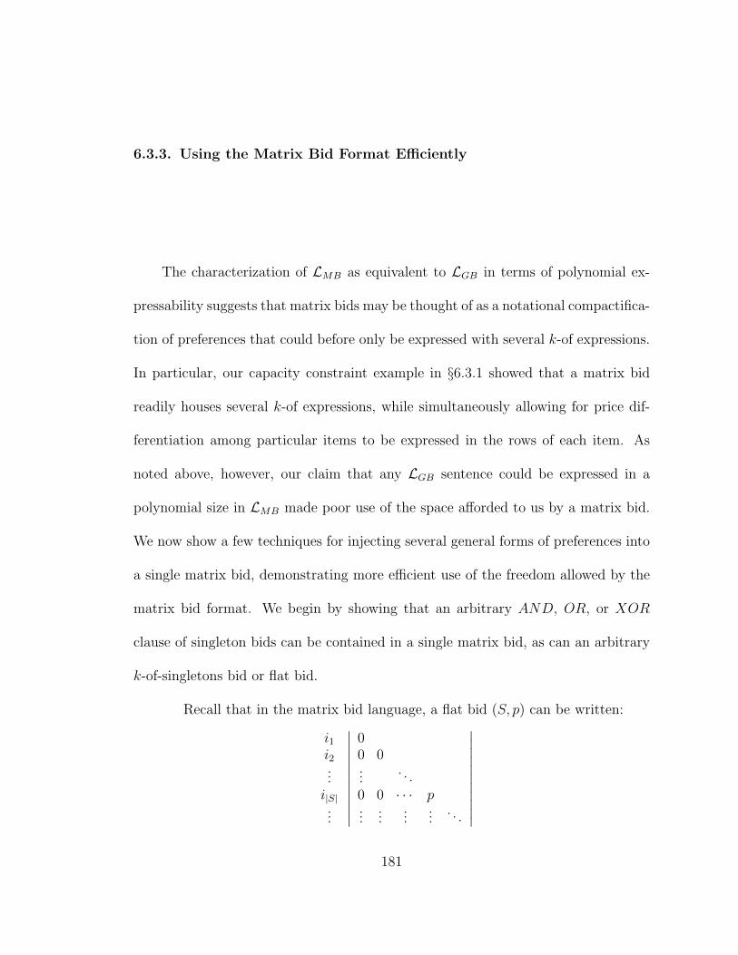
6.3.3. Using the Matrix Bid Format Efficiently
The characterization of LMB as equivalent to LGB in terms of polynomial ex-
pressability suggests that matrix bids may be thought of as a notational compactifica-
tion of preferences that could before only be expressed with several k-of expressions.
In particular, our capacity constraint example in §6.3.1 showed that a matrix bid
readily houses several k-of expressions, while simultaneously allowing for price dif-
ferentiation among particular items to be expressed in the rows of each item. As
noted above, however, our claim that any LGB sentence could be expressed in a
polynomial size in LMB made poor use of the space afforded to us by a matrix bid.
We now show a few techniques for injecting several general forms of preferences into
a single matrix bid, demonstrating more efficient use of the freedom allowed by the
matrix bid format. We begin by showing that an arbitrary AND, OR, or XOR
clause of singleton bids can be contained in a single matrix bid, as can an arbitrary
k-of-singletons bid or flat bid.
Recall that in the matrix bid language, a flat bid (S, p) can be written:
i1i2...
i|S|...
∣
∣
∣
∣
∣
∣
∣
∣
∣
∣
∣
00 0...
. . .0 0 · · · p...
......
.... . .
∣
∣
∣
∣
∣
∣
∣
∣
∣
∣
∣
181

where i1, i2, ...i|S| are the items in S written in any order, and the ellipses in this
example represent regions containing only zeros. This expression represents a very
inflexible offer, paid only if the exact package S is received.
A more flexible offer is demonstrated by the arbitrary OR bid, (i1 : p1 ∨ i2 :
p2 ∨ ...∨ in : pn) : b. Maintaining consistency with Boutillier [9], this bid offers pl for
item il taken in any combination with other items, and offers a bonus b if any one
of the items is awarded (i.e. if any of the singleton subclauses is satisfied). This OR
bid is captured in the matrix bid:
i1i2...in...
∣
∣
∣
∣
∣
∣
∣
∣
∣
∣
∣
p1 + bp2 + b p2
.... . .
pn + b pn · · · pn
......
......
. . .
∣
∣
∣
∣
∣
∣
∣
∣
∣
∣
∣
Here the items i1, i2, ...in in the OR statement are placed above (in higher ranked
rows) than items not in the statement, while again the ordering among the items
in the statement is inconsequential. We form this matrix bid by starting with an
additive valuation (a pl placed in every entry of the row for each il), and add the
bonus amount b to the first entry in each of these rows. This ensures that the bonus
must be awarded if at least one item in i1, i2, ...in is received, and is only awarded
once. The rows below in contain the items I\{i1, i2, ...in} and are filled with zeros.
Modeling the arbitrary AND of singleton bids combines the previous two
approaches. The LGB sentence (i1 : p1 ∧ i2 : p2 ∧ ... ∧ in : pn) : b offers an additive
182
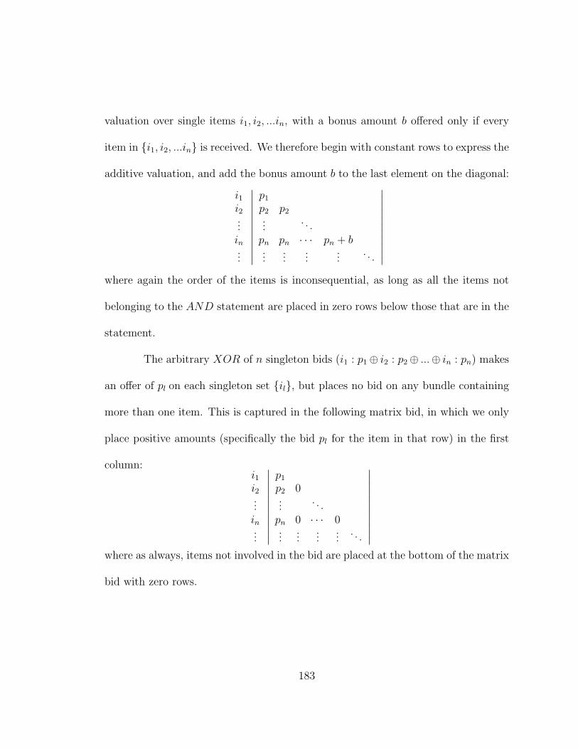
valuation over single items i1, i2, ...in, with a bonus amount b offered only if every
item in {i1, i2, ...in} is received. We therefore begin with constant rows to express the
additive valuation, and add the bonus amount b to the last element on the diagonal:
i1i2...in...
∣
∣
∣
∣
∣
∣
∣
∣
∣
∣
∣
p1
p2 p2...
. . .pn pn · · · pn + b...
......
.... . .
∣
∣
∣
∣
∣
∣
∣
∣
∣
∣
∣
where again the order of the items is inconsequential, as long as all the items not
belonging to the AND statement are placed in zero rows below those that are in the
statement.
The arbitrary XOR of n singleton bids (i1 : p1 ⊕ i2 : p2 ⊕ ...⊕ in : pn) makes
an offer of pl on each singleton set {il}, but places no bid on any bundle containing
more than one item. This is captured in the following matrix bid, in which we only
place positive amounts (specifically the bid pl for the item in that row) in the first
column:i1i2...in...
∣
∣
∣
∣
∣
∣
∣
∣
∣
∣
∣
p1
p2 0...
. . .pn 0 · · · 0...
......
.... . .
∣
∣
∣
∣
∣
∣
∣
∣
∣
∣
∣
where as always, items not involved in the bid are placed at the bottom of the matrix
bid with zero rows.
183

To model the k-of preference 〈k, S, p〉, a bid of p on at least k items from the
set S, consider the matrix bid:
i1i2.........
i|S|...
∣
∣
∣
∣
∣
∣
∣
∣
∣
∣
∣
∣
∣
∣
∣
∣
∣
∣
0 kth col
0. . . ↓
... p
... p. . .
......
.... . .
0 · · · p · · · · · ·. . .
......
......
.... . .
∣
∣
∣
∣
∣
∣
∣
∣
∣
∣
∣
∣
∣
∣
∣
∣
∣
∣
where the only non-zero entries are the values of p in the kth column in rows that
contain elements of S.
We note here that several k-of bids for the same set S can be contained in the
same matrix bid with “constant column” bids as illustrated in the previous example.
For example, if we have the bids 〈2, {a, b, c, d, e, f}, p2〉, 〈4, {a, b, c, d, e, f}, p4〉, and
〈5, {a, b, c, d, e, f}, p5〉, we would form the matrix bid:
abcdef
∣
∣
∣
∣
∣
∣
∣
∣
∣
∣
∣
00 p2
0 p2 00 p2 0 p4
0 p2 0 p4 p5
0 p2 0 p4 p5 0
∣
∣
∣
∣
∣
∣
∣
∣
∣
∣
∣
If at least two items are received the amount p2 is promised to the auctioneer, if at
least four items are received an additional amount p4 is promised, etc. If instead the
bidder wished to nest the exactly k-of bids [2, {a, b, c, d, e, f}, p2], [4, {a, b, c, d, e, f}, p4],
and [5, {a, b, c, d, e, f}, p5], she may use a similar technique, making sure that the sum
184

of the column values to the left of and including column k sum to the appropriate
amount:abcdef
∣
∣
∣
∣
∣
∣
∣
∣
∣
∣
∣
00 p2
0 p2 00 p2 0 p4 − p2
0 p2 0 p4 − p2 p5 − p4
0 p2 0 p4 − p2 p5 − p4 0
∣
∣
∣
∣
∣
∣
∣
∣
∣
∣
∣
In this case, if exactly four items are received then the second ranked item must have
been priced at p2 while the fourth ranked item must be priced at p4 − p2, summing
to the amount p4 as desired.
Just as several k-of bids can be nested in a single matrix bid, we now show
that a chain of flat bids (S1, p1), (S2, p2), ... (Sn, pn) with S1 ⊂ S2... ⊂ Sn can be
nested along the diagonal as in the following matrix bid:
S1
↓S2
↓...
Sn
↓...
∣
∣
∣
∣
∣
∣
∣
∣
∣
∣
∣
∣
∣
∣
∣
∣
∣
∣
0... p1
0p2 − p1
. . .0
pn − pn−1...
. . .
∣
∣
∣
∣
∣
∣
∣
∣
∣
∣
∣
∣
∣
∣
∣
∣
∣
∣
Here we have ordered the items so that all the items in S1 are ranked higher than all
the items in S2, which are all ranked higher than the items in S3, etc. We place the
bid of p1 for the set S1 on the diagonal in the row of the last (lowest ranked) element
in S1, and a bid of p2 − p1 in the row of the last element in set S2, so that receiving
all elements in S2 requires the acceptance of both bids p1 and p2 − p1, summing to
185

p2. Similarly, we put a bid of pl − pl−1 on the diagonal entry of the row with the
last element of Sl. It is easily verified that this matrix bid yields the appropriate
expression of preference, as assigning the last item in Sl causes the total accepted
bid to reach pl. We also notice that this bidder could assign bids for singleton sets in
the first column without damaging the preferences already expressed there, making
sure to reduce the diagonal entry containing p1by the amount of the singleton bid
on the item in the first row.
Because of its widespread use in simulations and general treatments of com-
binatorial auctions, it is interesting to consider the relationship of matrix bidding
to an XOR-of-flat-bids language. In particular, we are interested in the following
question: if a bidder can compute an optimal bid for any bundle and is given only
a limited number of matrix bids to convey her preferences, is there a way to fill in
matrix bid entries that makes safe (i.e. does not expose the bidder to paying too
much for a bundle) but effective (i.e. is not dominated by another safe value) use of
the space afforded by the matrix bid format?
Suppose, for example, that bidder j can quickly compute her desired bid on
any bundle, bj(S), and is filling out a matrix bid to convey her preferences. She may
first arrange the ranking of the auction items so that her most desired bundle is bid
on exactly on the diagonal, and then proceed to consider how to fill in the other
entries that are initially zero. Realizing that every bid on the diagonal and every
186
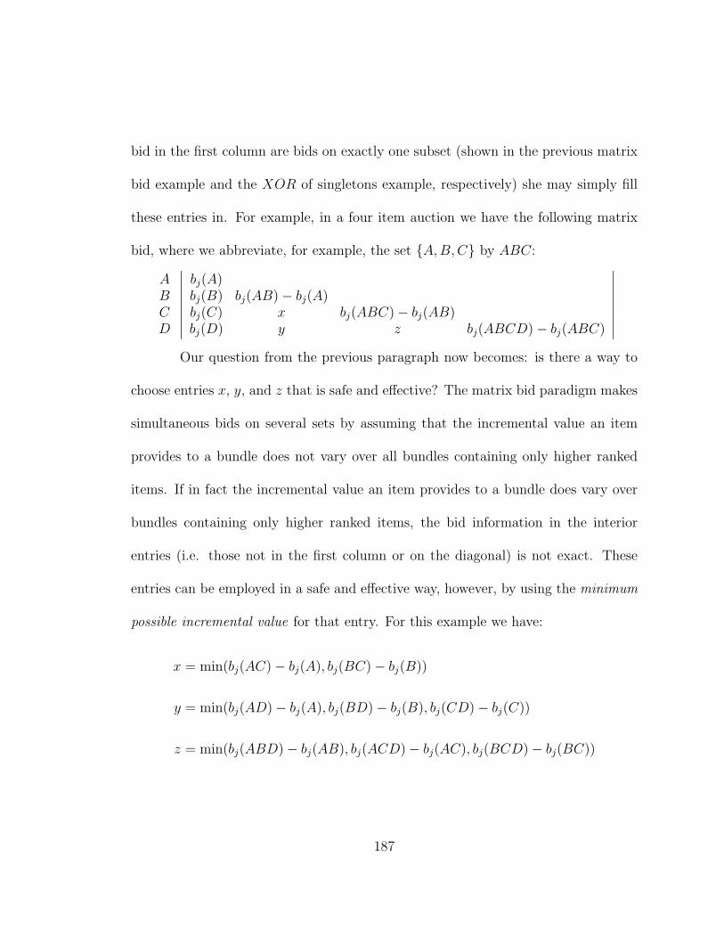
bid in the first column are bids on exactly one subset (shown in the previous matrix
bid example and the XOR of singletons example, respectively) she may simply fill
these entries in. For example, in a four item auction we have the following matrix
bid, where we abbreviate, for example, the set {A,B,C} by ABC:
ABCD
∣
∣
∣
∣
∣
∣
∣
∣
bj(A)bj(B) bj(AB) − bj(A)bj(C) x bj(ABC) − bj(AB)bj(D) y z bj(ABCD) − bj(ABC)
∣
∣
∣
∣
∣
∣
∣
∣
Our question from the previous paragraph now becomes: is there a way to
choose entries x, y, and z that is safe and effective? The matrix bid paradigm makes
simultaneous bids on several sets by assuming that the incremental value an item
provides to a bundle does not vary over all bundles containing only higher ranked
items. If in fact the incremental value an item provides to a bundle does vary over
bundles containing only higher ranked items, the bid information in the interior
entries (i.e. those not in the first column or on the diagonal) is not exact. These
entries can be employed in a safe and effective way, however, by using the minimum
possible incremental value for that entry. For this example we have:
x = min(bj(AC) − bj(A), bj(BC) − bj(B))
y = min(bj(AD) − bj(A), bj(BD) − bj(B), bj(CD) − bj(C))
z = min(bj(ABD) − bj(AB), bj(ACD) − bj(AC), bj(BCD) − bj(BC))
187

Filling in the corresponding matrix bid entries with these values assures that the
bidder has bid a safe amount, but could not have bid a higher safe amount. We note
the interesting property that the number of terms in each minimization corresponds
exactly to Pascal’s triangle [57]:
11 11 2 11 3 3 11 4 6 4 1...
. . .
This provides a characterization of the accuracy of each entry: bijk is an incremental
value for item i if added to any of the(
rij−1k−1
)
possible bundles containing k−1 more
highly ranked items. This emphasizes that bid accuracy is exact in the left column
and diagonal, and is least accurate in the middle of the bottom row. In general, this
technique of finding a safe value for an arbitrary entry is given by:
bsafeijk = min
S∈SB(i,j,k)bj(S ∪ i) − bj(S)
where SB(i, j, k) = {S ⊂ I|rıj < rij, ∀ı ∈ S, and |S| = k − 1}
This “safe bid” technique allows a bidder to safely “pack in” more bid in-
formation into a matrix bid with a particular ranking or ordering of items already
chosen. The method begins to answer the larger question of how to best use matrix
bids to convey a general bid function, but to solve this larger problem the bidder
must maximize bid accuracy over the N ! possible orderings, a problem that in general
188
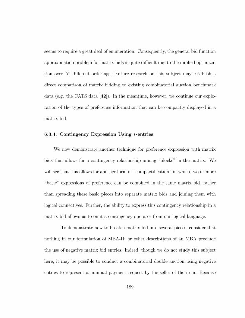
seems to require a great deal of enumeration. Consequently, the general bid function
approximation problem for matrix bids is quite difficult due to the implied optimiza-
tion over N ! different orderings. Future research on this subject may establish a
direct comparison of matrix bidding to existing combinatorial auction benchmark
data (e.g. the CATS data [42]). In the meantime, however, we continue our explo-
ration of the types of preference information that can be compactly displayed in a
matrix bid.
6.3.4. Contingency Expression Using ∗-entries
We now demonstrate another technique for preference expression with matrix
bids that allows for a contingency relationship among “blocks” in the matrix. We
will see that this allows for another form of “compactification” in which two or more
“basic” expressions of preference can be combined in the same matrix bid, rather
than spreading these basic pieces into separate matrix bids and joining them with
logical connectives. Further, the ability to express this contingency relationship in a
matrix bid allows us to omit a contingency operator from our logical language.
To demonstrate how to break a matrix bid into several pieces, consider that
nothing in our formulation of MBA-IP or other descriptions of an MBA preclude
the use of negative matrix bid entries. Indeed, though we do not study this subject
here, it may be possible to conduct a combinatorial double auction using negative
entries to represent a minimal payment request by the seller of the item. Because
189

this requires added structure in the IP formulation, we maintain our original focus
on a one-sided MBA, and save the study of a matrix bid double auction for future
research.
Within the context of a one-sided auction, however, we do consider negative
entries in one capacity: if a particular entry in a matrix bid is assigned a signifi-
cantly negative number, then the revenue maximization will never assign the item in
that row to the agent represented by that column. Representing this large negative
number as ∗, we can block off regions of a matrix bid forcing entries to only be
accepted in a certain way. We note that in practice we obtain the same results for
∗-entries by simply removing the decision variable associated with that entry from
the IP formulation. Also, we notice that the use of ∗ as a prohibitive bid disallowing
the acceptance of a certain bid is similar to the use of ∗ in our characterization of
exactly-k-of bids in terms of k-of bids above.
To demonstrate the use of ∗, consider a bidder who wishes to express a
contingency relationship between two “basic” valuations which can each be written in
its own matrix bid. Suppose, for example, that the bidder is interested in purchasing
a set of three items {A,B,C} as a package at a price of 40, and would like to express
an additive valuation over items {D,E, F} contingent upon winning the essential
set {A,B,C}. Using one block for the flat bid portion of these preferences and an
190
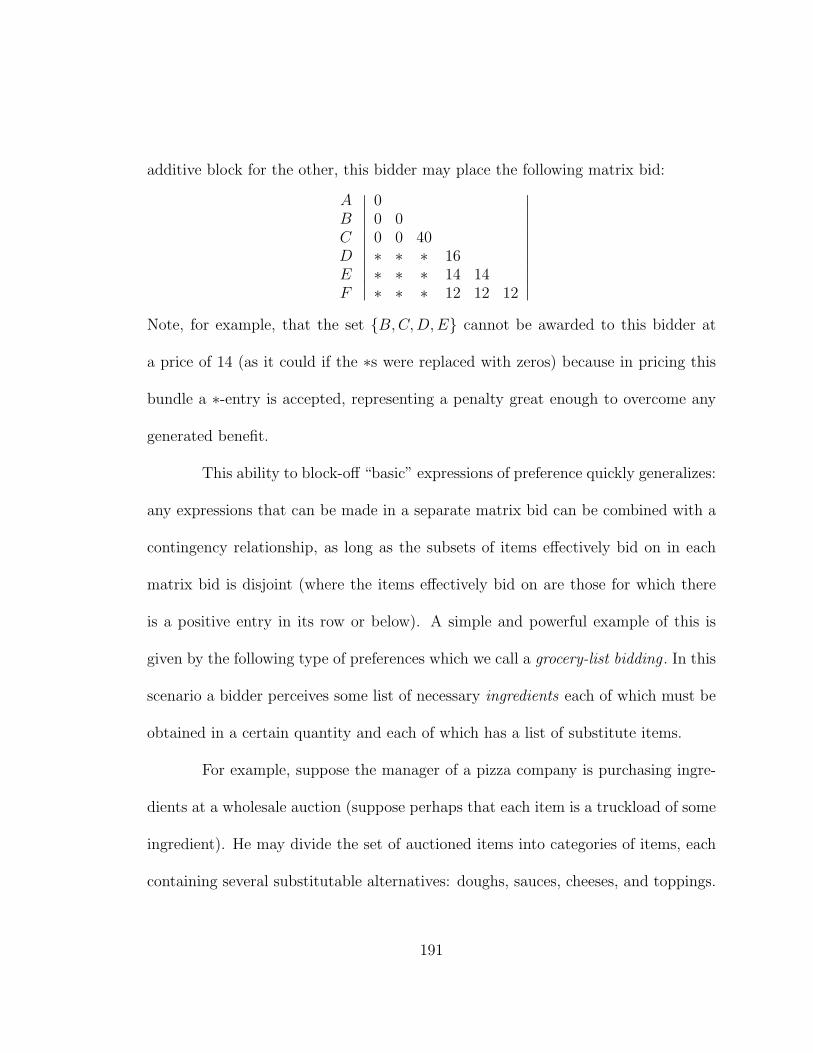
additive block for the other, this bidder may place the following matrix bid:
ABCDEF
∣
∣
∣
∣
∣
∣
∣
∣
∣
∣
∣
00 00 0 40∗ ∗ ∗ 16∗ ∗ ∗ 14 14∗ ∗ ∗ 12 12 12
∣
∣
∣
∣
∣
∣
∣
∣
∣
∣
∣
Note, for example, that the set {B,C,D,E} cannot be awarded to this bidder at
a price of 14 (as it could if the ∗s were replaced with zeros) because in pricing this
bundle a ∗-entry is accepted, representing a penalty great enough to overcome any
generated benefit.
This ability to block-off “basic” expressions of preference quickly generalizes:
any expressions that can be made in a separate matrix bid can be combined with a
contingency relationship, as long as the subsets of items effectively bid on in each
matrix bid is disjoint (where the items effectively bid on are those for which there
is a positive entry in its row or below). A simple and powerful example of this is
given by the following type of preferences which we call a grocery-list bidding . In this
scenario a bidder perceives some list of necessary ingredients each of which must be
obtained in a certain quantity and each of which has a list of substitute items.
For example, suppose the manager of a pizza company is purchasing ingre-
dients at a wholesale auction (suppose perhaps that each item is a truckload of some
ingredient). He may divide the set of auctioned items into categories of items, each
containing several substitutable alternatives: doughs, sauces, cheeses, and toppings.
191

Figure 6.2. A grocery-list Matrix Bid
dough Adough Bdough Cdough Dcheese Acheese Bcheese Ccheese Dsauce Asauce Bsauce C
topping Atopping Btopping C
∣
∣
∣
∣
∣
∣
∣
∣
∣
∣
∣
∣
∣
∣
∣
∣
∣
∣
∣
∣
∣
∣
∣
∣
∣
∣
∣
00 00 0 00 0 0 ∗∗ ∗ ∗ 0 ∗∗ ∗ ∗ 0 0 ∗∗ ∗ ∗ 0 0 ∗ ∗∗ ∗ ∗ 0 0 ∗ ∗ ∗∗ ∗ ∗ ∗ ∗ 40 ∗ ∗ ∗∗ ∗ ∗ ∗ ∗ 48 ∗ ∗ ∗∗ ∗ ∗ ∗ ∗ 52 ∗ ∗ ∗∗ ∗ ∗ ∗ ∗ ∗ 7 ∗ ∗∗ ∗ ∗ ∗ ∗ ∗ 6 6 ∗∗ ∗ ∗ ∗ ∗ ∗ 5 5 5
∣
∣
∣
∣
∣
∣
∣
∣
∣
∣
∣
∣
∣
∣
∣
∣
∣
∣
∣
∣
∣
∣
∣
∣
∣
∣
∣
Suppose further that his preferences are as follows. (i) He needs to obtain exactly
three of the four types of dough, two of the four types of cheese, and one of the
three types of sauce, or else he is not willing to purchase anything. (ii) Further, he
perceives different quality levels for the various sauces, making him willing to pay 8
additional monetary units if his bundle contains sauce B, and 12 units if his bundle
contains sauce C. (iii) Finally, he has additive preferences over three toppings, given
that he has a bundle that satisfies his dough, cheese and sauce requirements. His
preferences may be compactly expressed in the matrix bid Figure 6.2.
Applying the basic assumption for matrix bids that matrix bid entries may
only be accepted in a down and to the right fashion, it is easy to see that the
bid of Figure 6.2 expresses no positive bid except on bundles that contain exactly
192
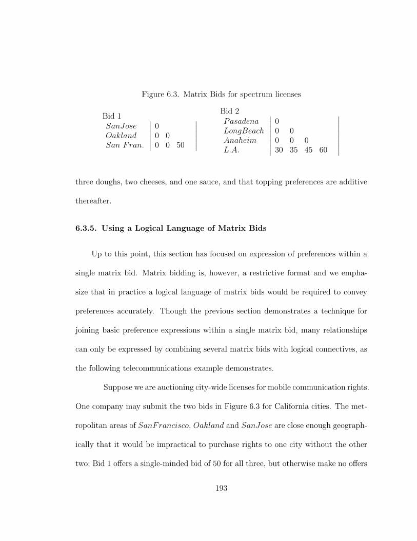
Figure 6.3. Matrix Bids for spectrum licenses
Bid 1SanJoseOaklandSan Fran.
∣
∣
∣
∣
∣
∣
00 00 0 50
∣
∣
∣
∣
∣
∣
Bid 2PasadenaLongBeachAnaheimL.A.
∣
∣
∣
∣
∣
∣
∣
∣
00 00 0 030 35 45 60
∣
∣
∣
∣
∣
∣
∣
∣
three doughs, two cheeses, and one sauce, and that topping preferences are additive
thereafter.
6.3.5. Using a Logical Language of Matrix Bids
Up to this point, this section has focused on expression of preferences within a
single matrix bid. Matrix bidding is, however, a restrictive format and we empha-
size that in practice a logical language of matrix bids would be required to convey
preferences accurately. Though the previous section demonstrates a technique for
joining basic preference expressions within a single matrix bid, many relationships
can only be expressed by combining several matrix bids with logical connectives, as
the following telecommunications example demonstrates.
Suppose we are auctioning city-wide licenses for mobile communication rights.
One company may submit the two bids in Figure 6.3 for California cities. The met-
ropolitan areas of SanFrancisco, Oakland and SanJose are close enough geograph-
ically that it would be impractical to purchase rights to one city without the other
two; Bid 1 offers a single-minded bid of 50 for all three, but otherwise make no offers
193
on any cities. Bid 2 introduces a different type of behavior. The bidding company is
most concerned with purchasing the rights to L.A., but feels that they will experience
increased returns for each of the neighboring cities they obtain. Furthermore, they
cannot support a communications network in the smaller neighboring cities without
at least controlling the hub, L.A. They bid 30 on L.A. by itself, 35 on L.A. with any
one of its neighbors, 45 on L.A. with any two of its neighbors, and 60 on L.A. with
all three of its neighbors. In general, if a bidder considers one item to be essential,
with a set of n other items as substitutable accessories or add-ons, she may make
bids on the distinguished item with 0 accessories, 1 accessory, . . . n accessories by
bidding with an increasing row (we call such a bidder an add-on bidder).
If the two bids in this example are treated as if the single bidder had two
bidders acting on his behalf, the submission is interpreted as “Bid 1 OR Bid 2”. The
OR is inclusive; the company submitting these bids may receive a subset which is the
union of subsets obtained by each of its matrix bids. They may receive, for example,
{SanJose,Oakland, SanFran.} ∪ {L.A., LongBeach} and pay 50 + 35 = 85 units
for the bundle. It may be the case, however, that the company is only interested in
purchasing the rights for one of the two regions; they wish to bid “Bid 1 XOR Bid
2”.
One way to quickly accomplish a XOR bid is to add a constraint on the
slack variables into the integer program MBA-IP. Observe that if slack variable
194
yj1 = 1, bidder j’s first agent is completely without an item. According to the
ordering constraints if there is no item at bidder j’s first agent there can be no item
in bidder j’s second agent, and so forth; yj1 = 1 therefore implies that bidder j
receives no items. Since each bidder represents a single matrix bid we may achieve
“Bid 1 XOR Bid 2” by adding the constraint:
y11 + y21 ≥ 1
where j = 1, 2 refer to Bid 1 and Bid 2 respectively. For the remainder of this
subsection we use the convention that each j ∈ J refers to a single matrix bid,
rather than a bidder in the auction.
In general the XOR of matrix bids 1, 2...m may be expressed by:
m∑
j=1
yj1 ≥ m − 1
If a bidder submits a request to XOR matrix bids 1, 2...m, and a separate request
to XOR matrix bids (m+1), (m+2)...n, these submissions do not mutually exclude
one another. This allows each bidder’s submission to easily take the general form:
(MatrixBid1 XOR MatrixBid2... XOR MatrixBid M1) OR
(MatrixBid M1 + 1 XOR ...MatrixBid M2) OR...
(MatrixBid MQ−1 + 1 XOR ...MatrixBid MQ)
195

specifying an OR-of-XOR of matrix bids language, where Mq =∑q
l=1 ml, and each
ml equals the number of XORed matrix bids in the lth of the Q different ORed
clauses.
Also studied in the auction literature are XOR-of-OR bidding languages,
which include the format initially proposed for the FCC’s Auction #31 [28]. This
can be modeled in the matrix bid language as follows. Add a binary variable for
each OR string, and define Q = {1, 2, ...Q} as the XORed set of clauses, each an
ORed string of matrix bids. A bidder’s complete preference submission will be of
the form:
(MatrixBid1 OR MatrixBid2... OR MatrixBid M1) XOR
(MatrixBid M1 + 1 OR ...MatrixBid M2) XOR...
(MatrixBid MQ−1 + 1 OR ...MatrixBid MQ)
where Mq =∑q
l=1 ml, and each ml is now equal to the number of ORed matrix
bids in the lth of the Q different XORed clauses. For each q ∈ Q define gq = 0 if
any matrix bid in the ORed string q receives items, gq = 1 otherwise. Then add
definitional constraints to MBA-IP for each string q:
gq ≤ yj1, ∀ j ∈ q
196
and the XOR constraint:Q
∑
q=1
gq ≥ Q − 1
The first constraint ensures that if gq = 1, then none of the matrix bids j in string q
receives items, while the second constraint ensures that among all Q strings at most
one has one or more matrix bids receiving items.
If instead we are interested in expressing a premium p that will be paid
only if some collection of statements each expressed in a matrix bid is satisfied, we
can form constraints based on the slack variables for the last agent in each matrix
bid that must be satisfied for the statement to be valid. For example, consider the
communication license example and suppose we want to express that a premium
p will be paid if the single-minded Bid1 is satisfied and at least two of the L.A.
neighbors in Bid2 are awarded. We can model this by introducing a new binary
decision variable hp which equals 1 whenever the AND of the two statements is
satisfied, and is zero otherwise. We now add the constraints:
y13 + hp ≤ 1
y23 + hp ≤ 1
197

and an objective term p · hp. The value of the premium p is therefore only allowed
to enter the objective function value when both agents receives items. The general-
ization of this technique to model a premium for the AND of more than two matrix
bids follows similarly.
Though we provide here several examples of potentially useful logical lan-
guages of matrix bids, many other are possible. Indeed, any of the logical bidding
structures put forth by Boutillier [9] may be adapted to create a more or less com-
plex logical language of matrix bids. Our examples show that in certain cases a
formulation may be expressed in terms of the slack variables for a single agent from
each matrix bid, rather than on a large collection of xijk assignment variables. We
note that the particular choice of an appropriate logical language may vary from
application to application, and that one direction for future research is to empiri-
cally measure the trade-off between expressability and computational burden in the
selection of a logical language.
198
CHAPTER 7
Computational Experiments for Matrix Bidding
After exploring the expressability of the matrix bids format as a compact
language for conveying a wide variety of preference information and categorizing
the winner determination problem for an MBA as NP-hard, we are interested to
see how efficiently we can solve instances of our formulation MBA-IP. In the early
phases of our investigation, we began with some small examples generated on an
ad-hoc basis, using our own imagination and economic intuition. Next we generated
problems randomly, selecting each entry in each matrix bid from the same set of
possible values with equal probability. Many of these instances were easily solved by
their LP relaxation, while a few trends appeared in the more difficult cases which
motivated the heuristics and data generation presented in this chapter.
In our examination of fractional LP-relaxation solutions, we investigated how
to generate valid inequalities (cuts) that eliminate such solutions. We noticed that
cover inequalities (commonly used for 0-1 Knapsack problems [47]) can be adapted
and applied to our formulation MBA-IP. In the context of matrix bids the concept
of a cover inequality can be described as follows. In an MBA each bidder has N
ranked agents. If agent (j, k) receives an item then bidder j receives at least k items.
199
Naturally then, for two or more agents from different bidders, if the sum of the k
indices of these agents is more than the number of items N , then one of these two
agents must not receive an item. For example in an MBA with N = 6, bidder 1’s 4th
agent and bidder 2’s 4th agent cannot both receive items. These conditions can be
expressed as linear inequalities which are satisfied by all integer solutions to MBA-
IP, but may be violated by fractional extreme points in its LP-relaxation. In §7.1.1
we develop a heuristic for the separation and application of these cover inequalities
which can be used to eliminate fractional solutions when identified.
The second trend we noticed in out initial attempts at winner determination
was that many LP-relaxations yielding a fractional solution often had the same
objective function value as the optimal integer solution. Coupling this with the
observation that the yjk variables are always non-decreasing in the value of k for a
given bidder j, we were motivated to develop an objective perturbation on the slack
variables yjk that favors integer solutions over fractional solutions in the presence of
multiple optima. This objective perturbation technique is described in §7.1.2.
In our initial experiments it was uncommon to find instances in which the
LP-relaxations yielded fractional solutions, and we decided that it would be benefi-
cial to generate simulated auction data in a more sophisticated way. The reasoning
for this was that the very “lumpy” preferences, those with significant positive syner-
gies, were not very likely under a scheme in which each matrix bid entry was drawn
200
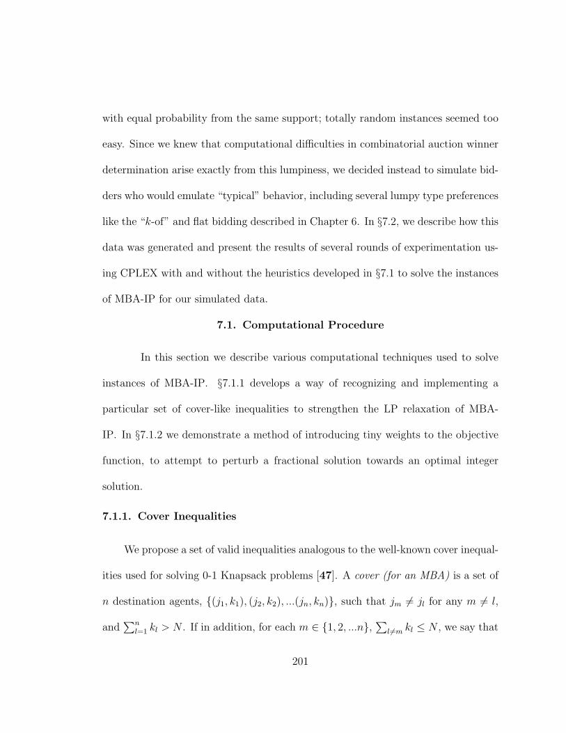
with equal probability from the same support; totally random instances seemed too
easy. Since we knew that computational difficulties in combinatorial auction winner
determination arise exactly from this lumpiness, we decided instead to simulate bid-
ders who would emulate “typical” behavior, including several lumpy type preferences
like the “k-of” and flat bidding described in Chapter 6. In §7.2, we describe how this
data was generated and present the results of several rounds of experimentation us-
ing CPLEX with and without the heuristics developed in §7.1 to solve the instances
of MBA-IP for our simulated data.
7.1. Computational Procedure
In this section we describe various computational techniques used to solve
instances of MBA-IP. §7.1.1 develops a way of recognizing and implementing a
particular set of cover-like inequalities to strengthen the LP relaxation of MBA-
IP. In §7.1.2 we demonstrate a method of introducing tiny weights to the objective
function, to attempt to perturb a fractional solution towards an optimal integer
solution.
7.1.1. Cover Inequalities
We propose a set of valid inequalities analogous to the well-known cover inequal-
ities used for solving 0-1 Knapsack problems [47]. A cover (for an MBA) is a set of
n destination agents, {(j1, k1), (j2, k2), ...(jn, kn)}, such that jm 6= jl for any m 6= l,
and∑n
l=1 kl > N . If in addition, for each m ∈ {1, 2, ...n},∑
l 6=m kl ≤ N , we say that
201
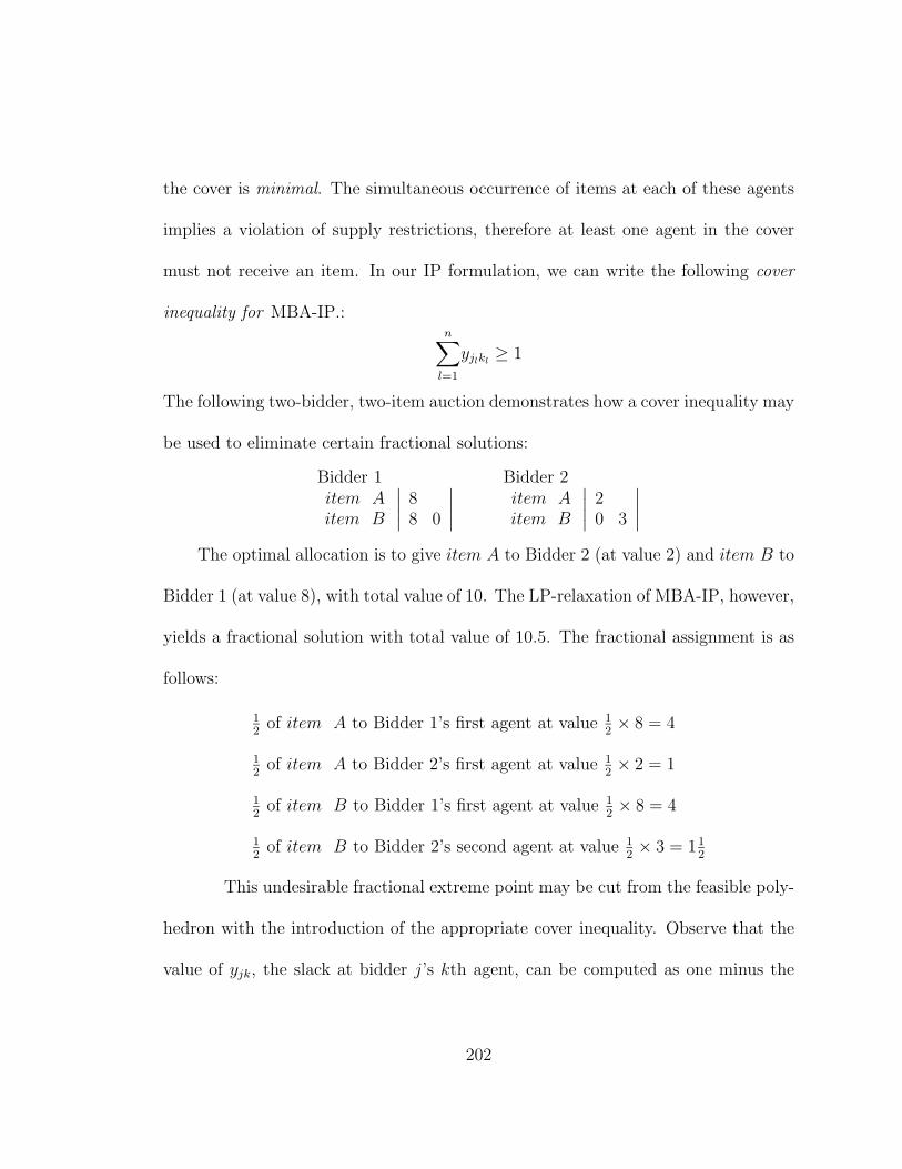
the cover is minimal. The simultaneous occurrence of items at each of these agents
implies a violation of supply restrictions, therefore at least one agent in the cover
must not receive an item. In our IP formulation, we can write the following cover
inequality for MBA-IP.:n
∑
l=1
yjlkl≥ 1
The following two-bidder, two-item auction demonstrates how a cover inequality may
be used to eliminate certain fractional solutions:
Bidder 1item Aitem B
∣
∣
∣
∣
88 0
∣
∣
∣
∣
Bidder 2item Aitem B
∣
∣
∣
∣
20 3
∣
∣
∣
∣
The optimal allocation is to give item A to Bidder 2 (at value 2) and item B to
Bidder 1 (at value 8), with total value of 10. The LP-relaxation of MBA-IP, however,
yields a fractional solution with total value of 10.5. The fractional assignment is as
follows:
12
of item A to Bidder 1’s first agent at value 12× 8 = 4
12
of item A to Bidder 2’s first agent at value 12× 2 = 1
12
of item B to Bidder 1’s first agent at value 12× 8 = 4
12
of item B to Bidder 2’s second agent at value 12× 3 = 11
2
This undesirable fractional extreme point may be cut from the feasible poly-
hedron with the introduction of the appropriate cover inequality. Observe that the
value of yjk, the slack at bidder j’s kth agent, can be computed as one minus the
202
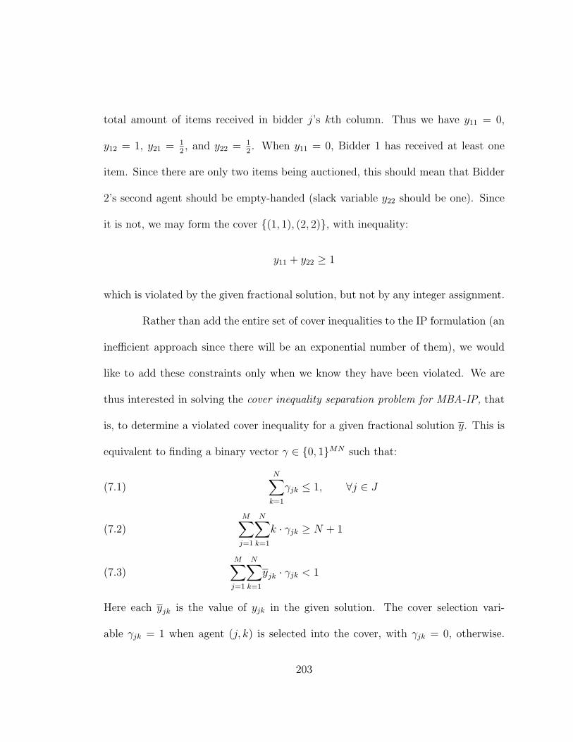
total amount of items received in bidder j’s kth column. Thus we have y11 = 0,
y12 = 1, y21 = 12, and y22 = 1
2. When y11 = 0, Bidder 1 has received at least one
item. Since there are only two items being auctioned, this should mean that Bidder
2’s second agent should be empty-handed (slack variable y22 should be one). Since
it is not, we may form the cover {(1, 1), (2, 2)}, with inequality:
y11 + y22 ≥ 1
which is violated by the given fractional solution, but not by any integer assignment.
Rather than add the entire set of cover inequalities to the IP formulation (an
inefficient approach since there will be an exponential number of them), we would
like to add these constraints only when we know they have been violated. We are
thus interested in solving the cover inequality separation problem for MBA-IP, that
is, to determine a violated cover inequality for a given fractional solution y. This is
equivalent to finding a binary vector γ ∈ {0, 1}MN such that:
N∑
k=1
γjk ≤ 1, ∀j ∈ J(7.1)
M∑
j=1
N∑
k=1
k · γjk ≥ N + 1(7.2)
M∑
j=1
N∑
k=1
yjk · γjk < 1(7.3)
Here each yjk is the value of yjk in the given solution. The cover selection vari-
able γjk = 1 when agent (j, k) is selected into the cover, with γjk = 0, otherwise.
203

Constraints (7.1) dictate that at most one agent is selected from each bidder, while
constraints (7.2) ensure that the selected agents indeed have k indices that sum to
strictly more than the number of auctioned items N (i.e. we have selected a cover).
Constraint (7.3) guarantees that the selected cover is in fact violated by the current
solution y.
In this section, we demonstrate a necessary condition for the existence of
a solution to this problem and introduce a heuristic technique for finding cover
inequalities (in lieu of solving this cover separation IP exactly). We also note that
because the cover inequalities defined here differ from the standard cover inequalities,
we may not apply typical separation heuristics.
We begin with the following observations:
Lemma 7.1. For any solution to the LP relaxation of MBA-IP,
M∑
j=1
N∑
k=1
yjk = N(M − 1)
Proof. Summing each of the N constraints from (6.1) (introduced in §6.2) yields
M∑
j=1
N∑
k=1
∑
i∈I|rij≥k
xijk = N
while summing each of the MN constraints in (6.2) yields
M∑
j=1
N∑
k=1
∑
i∈I|rij≥k
xijk +M
∑
j=1
N∑
k=1
yjk = MN
with the desired result following by subtraction. �
204
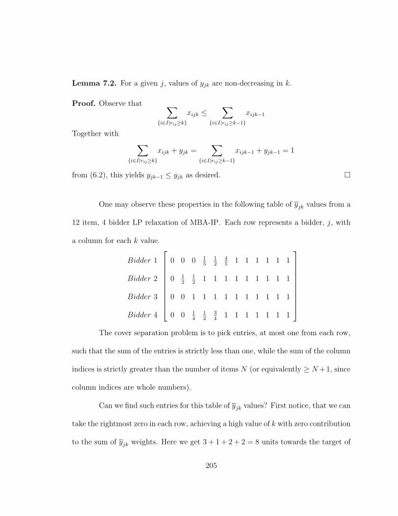
Lemma 7.2. For a given j, values of yjk are non-decreasing in k.
Proof. Observe that∑
{i∈I|rij≥k}
xijk ≤∑
{i∈I|rij≥k−1}
xijk−1
Together with∑
{i∈I|rij≥k}
xijk + yjk =∑
{i∈I|rij≥k−1}
xijk−1 + yjk−1 = 1
from (6.2), this yields yjk−1 ≤ yjk as desired. �
One may observe these properties in the following table of yjk values from a
12 item, 4 bidder LP relaxation of MBA-IP. Each row represents a bidder, j, with
a column for each k value.
Bidder 1
Bidder 2
Bidder 3
Bidder 4
0 0 0 15
12
45
1 1 1 1 1 1
0 12
12
1 1 1 1 1 1 1 1 1
0 0 1 1 1 1 1 1 1 1 1 1
0 0 14
12
34
1 1 1 1 1 1 1
The cover separation problem is to pick entries, at most one from each row,
such that the sum of the entries is strictly less than one, while the sum of the column
indices is strictly greater than the number of items N (or equivalently ≥ N +1, since
column indices are whole numbers).
Can we find such entries for this table of yjk values? First notice, that we can
take the rightmost zero in each row, achieving a high value of k with zero contribution
to the sum of yjk weights. Here we get 3 + 1 + 2 + 2 = 8 units towards the target of
205
13 (one more than N). As long there are some fractional values present, using these
rightmost zeros will never be enough to create a cover (since the sum of all (1− yjk)
values equals N and part of this sum lies in the fractional columns). Still, we have
simplified our problem now to finding fractional values whose improvements to the
cover total (i.e. the number of columns to the right of a rightmost zero) sum to at
least 13 − 8 = 5, while the sum of the selected entries sums to less than one. It is
now easy to verify by inspection that there is no way of selecting fractional values
from the table above, at most one per row, such that the values sum to less than
one, while the sum of the column distance each fractional value is away from the last
zero in its row is five or more.
The previous example provides some clues on how to find a violated cover in-
equality. To develop a general procedure, we compute a rating ρjk for each fractional
yjk, indicating how strong a candidate it is for entry into the cover:
ρjk =k − k∗
j
N + 1 − Z− yjk
where k∗j is the highest value of k for which yjk = 0, and Z is
∑M
j=1 k∗j , or equivalently,
the total number of yjk values equal to zero. When a row contains no zeros, we define
k∗j = 0.
By dividing k−k∗j , the number of columns away from a zero, by the amount
of contribution needed from the fractional values, N +1−Z, we have normalized the
problem so that a value’s simultaneous impact on both constraints can be measured.
206

Thus if ρjk > 0, yjk contributes proportionally more towards achieving the column
sum (of N + 1 − Z) than it adds to the total fractional weight, which must remain
below one. If ρjk < 0, then yjk contributes proportionally more to the fractional
weight than it does to achieving the desired column sum and is less likely to be an
appropriate choice.
We now show that if ρjk ≤ 0 for all (j, k) pairs, then no cover inequality is
violated.
Lemma 7.3. If a violated cover inequality exists then there exists a (j, k) pair in
the cover with ρjk > 0.
Proof. Suppose there is a violated cover inequality with ρjk ≤ 0 for all (j, k) in the
cover. Define γjk = 1 if (j, k) is in the cover, 0 otherwise. Starting from the
supposition that ρjk ≤ 0, we have:
ρjk ≤ 0 =⇒M
∑
j=1
N∑
k=1
γjk · ρjk =M
∑
j=1
N∑
k=1
γjk
k − k∗j
N + 1 − Z−
M∑
j=1
N∑
k=1
γjkyjk ≤ 0 =⇒
1
N + 1 − Z
M∑
j=1
N∑
k=1
γjk(k − k∗j ) ≤
M∑
j=1
N∑
k=1
γjkyjk < 1
with the last inequality holding because the specified cover is assumed to be violated.
Then
1
N + 1 − Z
M∑
j=1
N∑
k=1
γjk(k − k∗j ) < 1 =⇒
M∑
j=1
N∑
k=1
γjk(k − k∗j ) < N + 1 − Z
207
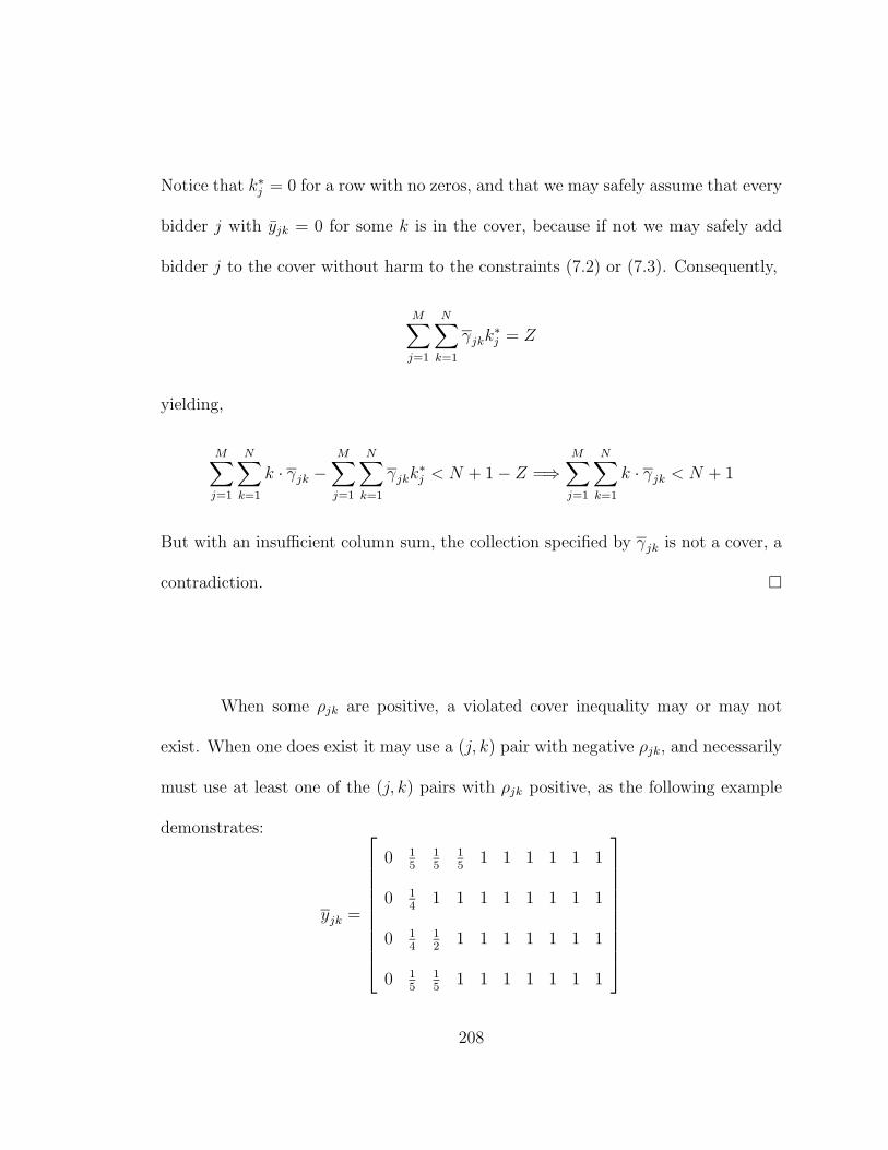
Notice that k∗j = 0 for a row with no zeros, and that we may safely assume that every
bidder j with yjk = 0 for some k is in the cover, because if not we may safely add
bidder j to the cover without harm to the constraints (7.2) or (7.3). Consequently,
M∑
j=1
N∑
k=1
γjkk∗j = Z
yielding,
M∑
j=1
N∑
k=1
k · γjk −M
∑
j=1
N∑
k=1
γjkk∗j < N + 1 − Z =⇒
M∑
j=1
N∑
k=1
k · γjk < N + 1
But with an insufficient column sum, the collection specified by γjk is not a cover, a
contradiction. �
When some ρjk are positive, a violated cover inequality may or may not
exist. When one does exist it may use a (j, k) pair with negative ρjk, and necessarily
must use at least one of the (j, k) pairs with ρjk positive, as the following example
demonstrates:
yjk =
0 15
15
15
1 1 1 1 1 1
0 14
1 1 1 1 1 1 1 1
0 14
12
1 1 1 1 1 1 1
0 15
15
1 1 1 1 1 1 1
208
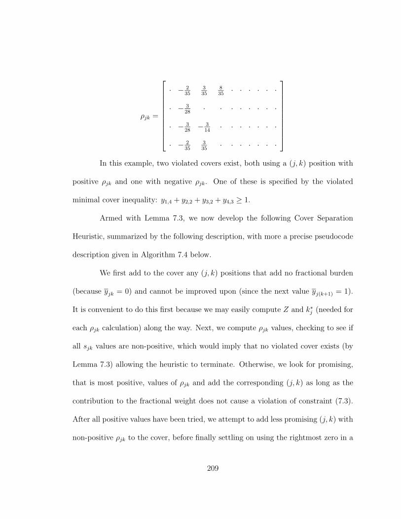
ρjk =
· − 235
335
835
· · · · · ·
· − 328
· · · · · · · ·
· − 328
− 314
· · · · · · ·
· − 235
335
· · · · · · ·
In this example, two violated covers exist, both using a (j, k) position with
positive ρjk and one with negative ρjk. One of these is specified by the violated
minimal cover inequality: y1,4 + y2,2 + y3,2 + y4,3 ≥ 1.
Armed with Lemma 7.3, we now develop the following Cover Separation
Heuristic, summarized by the following description, with more a precise pseudocode
description given in Algorithm 7.4 below.
We first add to the cover any (j, k) positions that add no fractional burden
(because yjk = 0) and cannot be improved upon (since the next value yj(k+1) = 1).
It is convenient to do this first because we may easily compute Z and k∗j (needed for
each ρjk calculation) along the way. Next, we compute ρjk values, checking to see if
all sjk values are non-positive, which would imply that no violated cover exists (by
Lemma 7.3) allowing the heuristic to terminate. Otherwise, we look for promising,
that is most positive, values of ρjk and add the corresponding (j, k) as long as the
contribution to the fractional weight does not cause a violation of constraint (7.3).
After all positive values have been tried, we attempt to add less promising (j, k) with
non-positive ρjk to the cover, before finally settling on using the rightmost zero in a
209
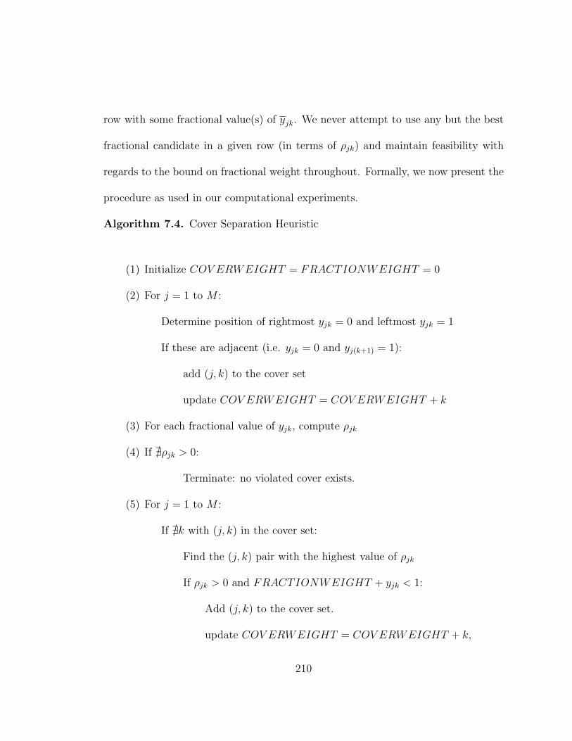
row with some fractional value(s) of yjk. We never attempt to use any but the best
fractional candidate in a given row (in terms of ρjk) and maintain feasibility with
regards to the bound on fractional weight throughout. Formally, we now present the
procedure as used in our computational experiments.
Algorithm 7.4. Cover Separation Heuristic
(1) Initialize COV ERWEIGHT = FRACTIONWEIGHT = 0
(2) For j = 1 to M :
Determine position of rightmost yjk = 0 and leftmost yjk = 1
If these are adjacent (i.e. yjk = 0 and yj(k+1) = 1):
add (j, k) to the cover set
update COV ERWEIGHT = COV ERWEIGHT + k
(3) For each fractional value of yjk, compute ρjk
(4) If ∄ρjk > 0:
Terminate: no violated cover exists.
(5) For j = 1 to M :
If ∄k with (j, k) in the cover set:
Find the (j, k) pair with the highest value of ρjk
If ρjk > 0 and FRACTIONWEIGHT + yjk < 1:
Add (j, k) to the cover set.
update COV ERWEIGHT = COV ERWEIGHT + k,
210
FRACTIONWEIGHT = FRACTIONWEIGHT + yjk
If COV ERWEIGHT ≥ N + 1:
Terminate: a violated cover has been found.
(6) For j = 1 to M :
If ∄k with (j, k) in the cover set:
Find the (j, k) pair with the highest value of ρjk
If FRACTIONWEIGHT + yjk < 1:
Add (j, k) to the cover set
update COV ERWEIGHT = COV ERWEIGHT + k,
FRACTIONWEIGHT = FRACTIONWEIGHT + yjk
If COV ERWEIGHT ≥ N + 1:
Terminate: a violated cover has been found.
(7) For j = 1 to M :
If ∄k with (j, k) in the cover set:
Add (j, k∗j ) to the cover set
update COV ERWEIGHT = COV ERWEIGHT + k∗j
If COV ERWEIGHT ≥ N + 1:
Terminate: a violated cover has been found.
(8) COV ERWEIGHT < N + 1
Terminate: the heuristic has failed to find a violated cover.
211
7.1.2. Objective Perturbation
After finding a solution to the LP-relaxation of MBA-IP and re-optimizing after
the addition of violated cover inequalities, the solution may still not correspond to
an integer allocation. In early experiments, we often found that the LP-relaxation
objective value was equal to the optimal integer objective function value; in many
cases there may be several solutions, both integer and fractional, on the optimal facet
of the feasible polyhedron. When branch-and-bound is used to iteratively solve LPs,
finding an integer extreme point among the numerous fractional extreme points on
the optimal facet can be very time consuming. In this section we suggest a technique
for making tiny shifts (or perturbations) to the objective function in order to favor
the integer extreme points among all optimal solutions to an LP-relaxation (possibly
after the addition of cover inequalities).
Recall from the discussion of cover inequalities that many fractional solutions
have fractional slack variables yjk, while every integer solution must have integer ys.
Recall also that for a given j, values of yjk are non-decreasing in k. Suppose we
place a tiny negative weight on each slack variable that is increasingly negative for
lower values of k. If we re-solve the LP relaxation, an integer solution with slack on
the lower values of k is favored over a fractional solution which has some slack on
yjks with higher values of k. This tiny penalty on higher values of k allows us to
favor integer solutions over fractional solutions that have the same objective value
212

without the penalty. At times this objective perturbation is enough to achieve the
optimal integer solution; in some instances it merely provides a better starting basis
for branch-and-bound (sometimes a drastically better basis).
Given a particular LP-relaxation solution with associated yjk values, we add
objective function coefficient δjk for each yjk, where:
δjk =(yjk − 1)
2N
If yjk = 0, yjk receives the most negative weight and is thus discouraged
from being set to anything other than zero. When yjk = 1 the weight is zero, and
there is no pressure to set yjk to zero. In between, larger fractional values of yjk
incur less negative weight than small values, achieving the desired effect.
This procedure may be performed iteratively; after each LP-solution is ob-
tained recompute the δjks and re-optimize. What happens if an integer solution
is found? The next calculation of perturbations will produce δjk = − 12N
wherever
yjk = 0, and δjk = 0 wherever yjk = 1. Since this will not change the objective
value of the previous integer solution, the ensuing LP optimization will return the
same solution. It is therefore safe to take a repeated solution as a stopping criterion
for iterative perturbation; you cannot perturb to an integer solution and then away
from it.
213
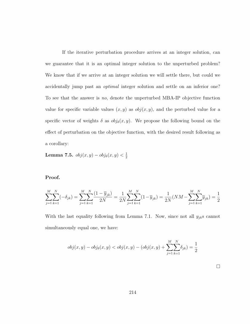
If the iterative perturbation procedure arrives at an integer solution, can
we guarantee that it is an optimal integer solution to the unperturbed problem?
We know that if we arrive at an integer solution we will settle there, but could we
accidentally jump past an optimal integer solution and settle on an inferior one?
To see that the answer is no, denote the unperturbed MBA-IP objective function
value for specific variable values (x, y) as obj(x, y), and the perturbed value for a
specific vector of weights δ as objδ(x, y). We propose the following bound on the
effect of perturbation on the objective function, with the desired result following as
a corollary:
Lemma 7.5. obj(x, y) − objδ(x, y) < 12
Proof.
M∑
j=1
N∑
k=1
(−δjk) =M
∑
j=1
N∑
k=1
(1 − yjk)
2N=
1
2N
M∑
j=1
N∑
k=1
(1−yjk) =1
2N(NM−
M∑
j=1
N∑
k=1
yjk) =1
2
With the last equality following from Lemma 7.1. Now, since not all yjks cannot
simultaneously equal one, we have:
obj(x, y) − objδ(x, y) < obj(x, y) − (obj(x, y) +M
∑
j=1
N∑
k=1
δjk) =1
2
�
214

Corollary 7.6. If the perturbation procedure terminates with integer variable values
(x, y), then (x, y) is an optimal integer solution of MBA-IP.
Proof. Suppose not. Let (x0, y0) be an optimal integer solution to MBA-IP. Since
(x, y) is not an optimal integer solution to MBA-IP by assumption, obj(x0, y0) >
obj(x, y), or equivalently obj(x0, y0)−1 ≥ obj(x, y) by integrality of the variables and
objective function coefficients. Lemma 7.5 provides objδ(x0, y0) > obj(x0, y0) −12
>
obj(x0, y0) − 1, which transitively tells us that objδ(x0, y0) > obj(x, y) ≥ objδ(x, y),
the last inequality following because all perturbation weights are non-positive. But
now this says objδ(x0, y0) > objδ(x, y), regardless of the choice of δ, thus the pertur-
bation procedure cannot terminate with variable values (x, y), since (x0, y0) yields a
better objective value for any δ. Thus we have reached a contradiction. �
Our approach is to iteratively perturb the objective function until a basis
is repeated (with a reasonable bound on the number of iterations). If the solution
obtained is integer Corollary 3.2 tells us that we are satisfied with this solution,
and the perturbation has assuredly served us well. When the solution obtained
from perturbation still has fractional variable values, we simply return the perturbed
objective coefficients to zero and initiate branch-and-bound, maintaining the current
solution. Though this would seem to imply that the objective perturbation was
unsuccessful, our experimental results indicate that the new solution can significantly
reduce the amount of time spent in the final branch-and-bound phase of optimization.
215
7.2. Experiments with Simulated Data
We report on our computational experiments and briefly describe our method
of data simulation. The purpose of these experiments is to explore the efficacy of our
computational techniques, to demonstrate the strength of the MBA-IP formulation,
and verify that we can indeed rapidly solve MBA instances. To achieve these goals,
data must be generated randomly, as little empirical data is publicly available for
actual combinatorial auctions. The type of data simulation used here is common in
the combinatorial auction literature. Sandholm et al.[65] is a prominent example,
while Boutillier [9] notes that the available benchmark data (e.g. the CATS test suite
discussed in [41]) is not beneficial for the testing of new language paradigms. There-
fore as in [9], we use random generation of “typical sentences” in our own language
as a test-bed for an initial evaluation of our ability to solve winner determination
problems stated in this language.
Since many available combinatorial auction techniques focus on flat atomic
bids and preferences built as an aggregation of flat bids, the data generated to
test these techniques is naturally comprised of randomly drawn bids attached to
randomly drawn subsets or bundles of items. Since matrix bidding is an auction
format in which bidders assign values to bundles in a more orderly fashion, it should
seem natural that our method is to randomly simulate expected behavior patterns.
Our simulations proceed under the assumption that each bidder is of a type randomly
216
drawn from each of the following seven types, which we use in an ad-hoc fashion to
simulate the presence of a variety of different bidders in the market.
• Additive Preference Bidder
• Single-Minded Bidder
• Nested Flat-Bid Bidder
• Nested k-of Bidder
• Partition Bidder
• Add-on Bidder
• Diminishing Returns Bidder
To maintain simplicity in our experiments, we restrict to the situation in
which each bidder is allowed only a single matrix bid (e.g. there is no XORing
of matrix bids.) The input for each set of experimental runs is N (the number of
items), M (the number of matrix bids), H (a parameter bounding the highest bid
per item), and A (the number of auctions to simulate with these parameters).
Using these parameters, the simulation first randomly selects a bid profile for
each matrix bid from one of the seven types described below with equal probability.
For each bid type a subroutine randomly selects a nonnegative integer for each of
the appropriate matrix bid entries based on the value H. We now describe how this
is achieved for each of the seven bidder types used in our experiments. In each case
217
(except for the partition bidder), before the entries in a matrix bid are filled in, a
ranking rij is chosen at random from among the N ! possibilities.
Additive Preference Bidder: For each item in the auction, an integer is chosen
from the set {0, 1, 2, ..., H} with equal probability. Every row is then filled in with
the same number equal to value chosen for the item in that row.
Single-minded Bidder: Included to simulate very inflexible or lumpy preferences,
this bidder places a single positive entry on the diagonal. A column is chosen at
random with equal probability, and a seed for the entry is chosen from the set
{1, 2, ..., H} with equal probability. The seed is then multiplied by the column num-
ber to reflect the number of items it is effectively bidding on.
Nested Flat-Bid Bidder: For each entry on the diagonal, an integer is chosen
from the set {−H, ..., H} with equal probability. Next, every negative selection is
set to equal zero; there is thus a H2H+1
probability of a positive entry, and probability
of 1H
for each positive value conditional upon the entry being positive. Finally each
positive entry is multiplied by the number of zero entries preceding it along the
diagonal, weighting each entry by the number of items it has effectively bid on.
Nested k-of Bidder: Begin with a nested flat-bid bidder and simply fill in each
column with the entry chosen for the diagonal entry in that column. An example is
given by Figure 7.1. If the numbers 6, 4, and 7 are drawn for the columns 3, 5, and
6, respectively, each column generated by multiplying the random number by the
218
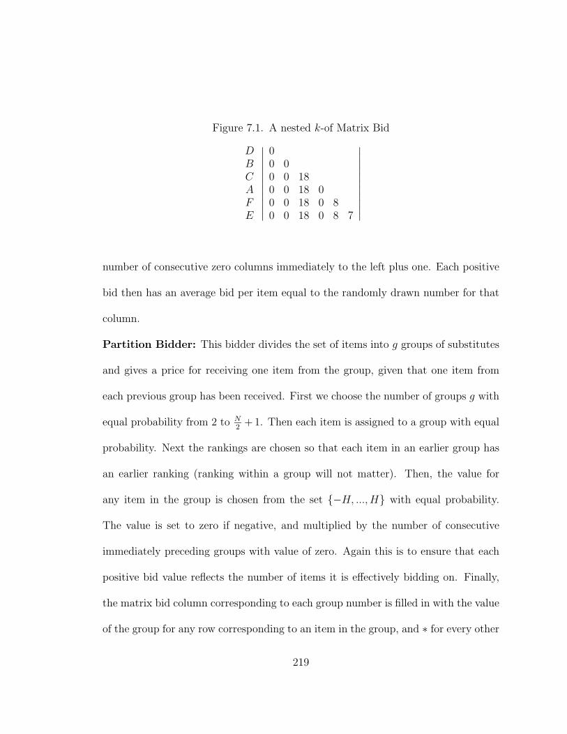
Figure 7.1. A nested k-of Matrix Bid
DBCAFE
∣
∣
∣
∣
∣
∣
∣
∣
∣
∣
∣
00 00 0 180 0 18 00 0 18 0 80 0 18 0 8 7
∣
∣
∣
∣
∣
∣
∣
∣
∣
∣
∣
number of consecutive zero columns immediately to the left plus one. Each positive
bid then has an average bid per item equal to the randomly drawn number for that
column.
Partition Bidder: This bidder divides the set of items into g groups of substitutes
and gives a price for receiving one item from the group, given that one item from
each previous group has been received. First we choose the number of groups g with
equal probability from 2 to N2
+ 1. Then each item is assigned to a group with equal
probability. Next the rankings are chosen so that each item in an earlier group has
an earlier ranking (ranking within a group will not matter). Then, the value for
any item in the group is chosen from the set {−H, ..., H} with equal probability.
The value is set to zero if negative, and multiplied by the number of consecutive
immediately preceding groups with value of zero. Again this is to ensure that each
positive bid value reflects the number of items it is effectively bidding on. Finally,
the matrix bid column corresponding to each group number is filled in with the value
of the group for any row corresponding to an item in the group, and ∗ for every other
219
row. The result is a special case of the grocery-list bidding from §6.3.4, in which
only one item is demanded from each group of substitutes.
Add-on Bidder: This bidder bids on an essential item and some nonnegative
amount for any number of add-on items. First the row of the item to be considered
essential is chosen at random with equal probability. Next an initial value is chosen
for the essential item which is placed in the first column of the row. For each following
entry in the row an integer between zero and the initial value is chosen, and added
to the previous value in the row until the row is filled.
Diminishing Returns Bidder: This bidder simulates weakly diminishing marginal
returns for every item received, and thus is generated to have weakly decreasing rows
and columns. The entry in the first row and first column (i.e., the value for the highest
ranked item) is chosen from {0, 1, 2, ..., H} with equal probability. Each entry in the
first column is given a value between the value above it and half of that value, with
a 50% probability of being equal to the entry above it and an equal probability of
taking any integer value between if not equal. To start the next column once a
column is filled, the diagonal entry from that column is generated in the same way,
but adjusting down to the entry on its left if that number is smaller. The other
entries in the new column are generated in the same way as the first column, based
on the entry above, but now adjusted down to the value of the entry on its left if
necessary to ensure weakly decreasing rows.
220
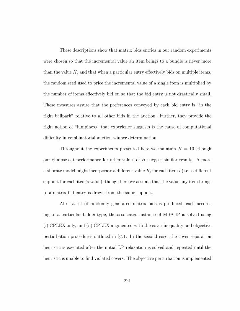
These descriptions show that matrix bids entries in our random experiments
were chosen so that the incremental value an item brings to a bundle is never more
than the value H, and that when a particular entry effectively bids on multiple items,
the random seed used to price the incremental value of a single item is multiplied by
the number of items effectively bid on so that the bid entry is not drastically small.
These measures assure that the preferences conveyed by each bid entry is “in the
right ballpark” relative to all other bids in the auction. Further, they provide the
right notion of “lumpiness” that experience suggests is the cause of computational
difficulty in combinatorial auction winner determination.
Throughout the experiments presented here we maintain H = 10, though
our glimpses at performance for other values of H suggest similar results. A more
elaborate model might incorporate a different value Hi for each item i (i.e. a different
support for each item’s value), though here we assume that the value any item brings
to a matrix bid entry is drawn from the same support.
After a set of randomly generated matrix bids is produced, each accord-
ing to a particular bidder-type, the associated instance of MBA-IP is solved using
(i) CPLEX only, and (ii) CPLEX augmented with the cover inequality and objective
perturbation procedures outlined in §7.1. In the second case, the cover separation
heuristic is executed after the initial LP relaxation is solved and repeated until the
heuristic is unable to find violated covers. The objective perturbation is implemented
221

Figure 7.2. Average run time for winner determination
M = 5 10 25 50 75 100N = 5 0.024 0.038 0.065 0.137 0.213 0.272
10 0.071 0.140 0.339 0.579 0.866 1.22225 2.812 1.967 3.890 11.035 14.098 22.73950 34.022 29.208 134.24 587.43 1192.9 2451.66
following the cover inequalities procedure, since it is clearly rewarding to tightly char-
acterize the feasible region (i.e. reduce it as much as possible) before perturbing. If
these methods do not produce an integer solution, we commence branch-and-bound
to determine an integer optimal solution, using CPLEX’s default branch-and-bound
settings.
This procedure of solving the same winner determination problem two dif-
ferent ways is then repeated for A different simulated auctions. In the first round of
experiments we set A = 10 for each value of (N,M) and examined the average, min-
imum, and maximum amount of computational time over the ten simulated auctions
for each method. Only ten auctions were used at each point to quickly ascertain
some global trends over a large number of points in (N,M) space. We repeated the
procedure of ten auctions for every combination of N taken from {5, 10, 15, ...50},
and M taken from {5, 10, 15, ...100} (since the size of the IP-formulation grows lin-
early in M and quadratically in N it seemed natural to be a bit more restrictive in
our choices of N .)
222
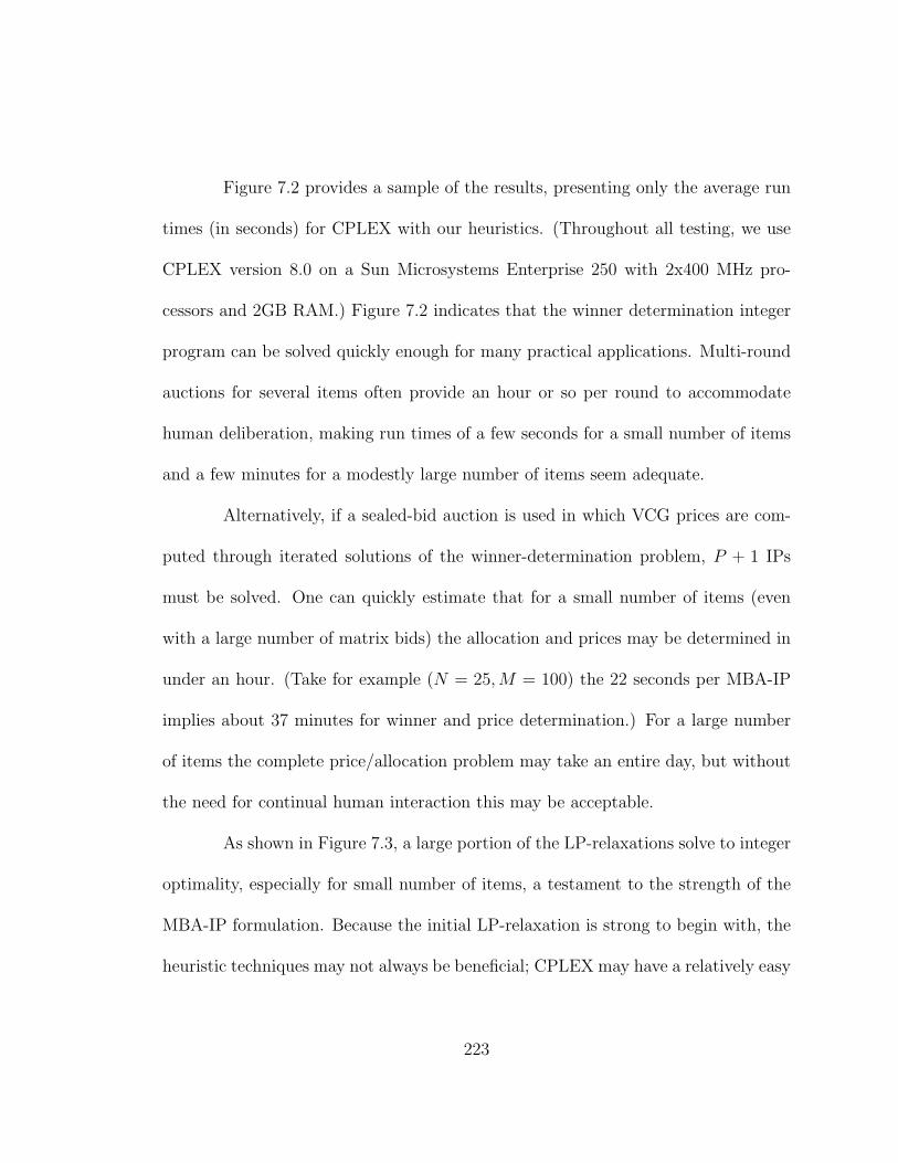
Figure 7.2 provides a sample of the results, presenting only the average run
times (in seconds) for CPLEX with our heuristics. (Throughout all testing, we use
CPLEX version 8.0 on a Sun Microsystems Enterprise 250 with 2x400 MHz pro-
cessors and 2GB RAM.) Figure 7.2 indicates that the winner determination integer
program can be solved quickly enough for many practical applications. Multi-round
auctions for several items often provide an hour or so per round to accommodate
human deliberation, making run times of a few seconds for a small number of items
and a few minutes for a modestly large number of items seem adequate.
Alternatively, if a sealed-bid auction is used in which VCG prices are com-
puted through iterated solutions of the winner-determination problem, P + 1 IPs
must be solved. One can quickly estimate that for a small number of items (even
with a large number of matrix bids) the allocation and prices may be determined in
under an hour. (Take for example (N = 25,M = 100) the 22 seconds per MBA-IP
implies about 37 minutes for winner and price determination.) For a large number
of items the complete price/allocation problem may take an entire day, but without
the need for continual human interaction this may be acceptable.
As shown in Figure 7.3, a large portion of the LP-relaxations solve to integer
optimality, especially for small number of items, a testament to the strength of the
MBA-IP formulation. Because the initial LP-relaxation is strong to begin with, the
heuristic techniques may not always be beneficial; CPLEX may have a relatively easy
223
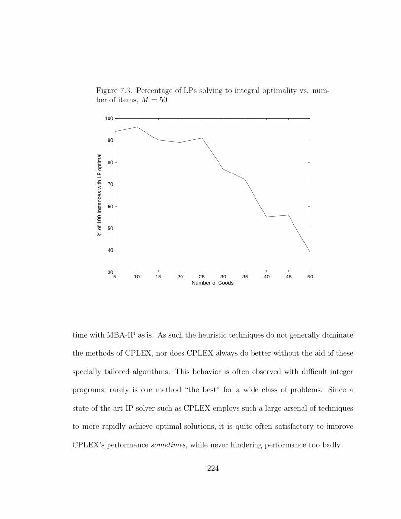
Figure 7.3. Percentage of LPs solving to integral optimality vs. num-ber of items, M = 50
5 10 15 20 25 30 35 40 45 5030
40
50
60
70
80
90
100
Number of Goods
% o
f 100
Inst
ance
s w
ith L
P o
ptim
al
time with MBA-IP as is. As such the heuristic techniques do not generally dominate
the methods of CPLEX, nor does CPLEX always do better without the aid of these
specially tailored algorithms. This behavior is often observed with difficult integer
programs; rarely is one method “the best” for a wide class of problems. Since a
state-of-the-art IP solver such as CPLEX employs such a large arsenal of techniques
to more rapidly achieve optimal solutions, it is quite often satisfactory to improve
CPLEX’s performance sometimes, while never hindering performance too badly.
224

Figure 7.4. Worst case run time vs. number of matrix bids, N = 50
0 10 20 30 40 50 60 70 800
10
20
30
40
50
60
Number of Matrix Bids
Tim
e (s
ec)
CPLEXCovers & Perturb
Figure 7.4 illustrates this sometimes improvement with a cross-section of
worst-case run times holding the number of items constant at 25 (taken from the
same data as above). The higher dotted peaks in this cross-section of data show that
the addition of specialized cover inequalities and objective perturbation potentially
diminish run time, while a solid peak above a dotted peak indicate that time spent
on the heuristics may not always be advantageous. Typically, however, run times
with and without the heuristics are similar.
225
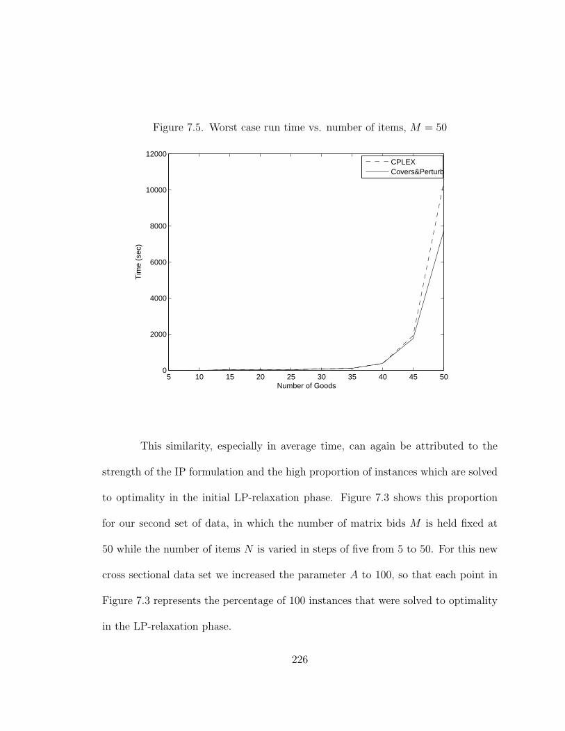
Figure 7.5. Worst case run time vs. number of items, M = 50
5 10 15 20 25 30 35 40 45 500
2000
4000
6000
8000
10000
12000
Number of Goods
Tim
e (s
ec)
CPLEXCovers&Perturb
This similarity, especially in average time, can again be attributed to the
strength of the IP formulation and the high proportion of instances which are solved
to optimality in the initial LP-relaxation phase. Figure 7.3 shows this proportion
for our second set of data, in which the number of matrix bids M is held fixed at
50 while the number of items N is varied in steps of five from 5 to 50. For this new
cross sectional data set we increased the parameter A to 100, so that each point in
Figure 7.3 represents the percentage of 100 instances that were solved to optimality
in the LP-relaxation phase.
226
This second set of data provides a more accurate comparison of worst-case
run times while holding the number of bidders constant. We see in Figure 7.5 that
the occasional differences between the two methods are smoothed out, and that in
the worst case the two methods perform about the same. We do see the heuristics
beginning to show more significant improvement for the largest instances, with a
difference of about 45 minutes in the worst instance overall. Still, the apparent
exponential growth in Figure 7.5 (typical of NP-hard problems) suggests that in a
multi-round setting MBA-IP would seem to be limited to auctions of 40 items or
less, with the heuristics helping to shave at best 30% off the computational time of
a run.
227
CHAPTER 8
Conclusions
Combinatorial auctions promise to increase efficiency and reduce exposure
risk in an economic environment where “synergy” is significant. Applications for
which combinatorial auctions achieve more desirable outcomes than traditional mar-
ket mechanisms abound in both governmental allocation problems and B2B com-
merce, as discussed in §2.1. This increased satisfaction in market outcomes comes
at the cost of computational difficulty, and the design of markets which quickly and
easily achieve beneficial outcomes is certain to provide interesting new avenues of
applied mathematics research for years to come.
With several potentially rewarding approaches to choose from (outlined in
Chapter 2), this dissertation focuses primarily on the bidder’s exponential bun-
dles problem, asking: how can simple compact representations of preference (price-
vectors) be combined to form more elaborate statements of preference? This ques-
tion follows somewhat naturally from the economic literature of Kelso and Crawford
[33], who introduce unit-demand bidders, each with preferences described by a price-
vector, in a model of the job-market, in which an employee can accept at most one
job. Kelso and Crawford [33] also introduce the gross substitutes property, which
228

has become fundamental in the study of auctions. The strength of this concept in
categorizing preferences and guaranteeing the existence of a unique Walrasian linear-
price equilibria has influenced several authors, including Ausubel and Milgrom [5],
and Gul and Stacchetti [26][27], all of whom provide foundational work for the re-
search presented here. Other results on unit-demand bidders are given by Demange,
Gale and Sotomayor [19], leading naturally into our own investigation of bid tables
in Chapter 3. Indeed, the case of unit-demand bidders is well studied, and we note
that our own Theorems 3.1 and 3.5 generalize the results of Demange, Gale and
Sotomayor (as presented, for example, in §8.3 of Roth and Sotomayor [60]), from
the case of unit-demand bidders to the case in which each bidder is represented by
multiple unit-demand agents.
Representing bidders by multiple unit-demand agents results in the fairly
natural and easy-to-read bid table format, causing us to wonder, why hasn’t this
been investigated before? We note that among the incentive properties of their
unit-demand bidder auction model, Roth and Sotomayor [60] show that a bidder
cannot benefit from shill bidding (having someone else join the auction to distort
its outcome). This may seem to imply that representing a bidder by multiple unit-
demand agents would be unrewarding, but the model under which this property
was proven maintains the assumption of a unit-demand valuation function for each
229

bidder. We, on the other hand, find use for the bid table format within the more
general context of multi-unit demand.
How general is the preference expression afforded by the bid table format
in the multi-unit demand context? Theorem 3.1 and Corollary 3.2 provide an exact
characterization: assignment preferences (those which can be written in bid tables)
are properly contained in the class of gross substitutes valuation functions. Ap-
plying a result of Gul and Stacchetti [26] based on this characterization, the gross
substitutes property elucidates the greatest strength of a bid table auction: unique
lowest Walrasian equilibrium price signals can be computed at each round of sub-
mission. The computation of these attractive linear price signals is facilitated by
our constrained optimization approach, which allows us to recognize and neutralize
“self-competition” constraints, overcoming the failure of the Hungarian algorithm to
provide the truly lowest Walrasian equilibrium prices in this context, as it does in
the unit-demand bidder context. With Theorems 3.4 and 3.5 we demonstrate the
computation of these price signals in each round or static instance using the tools
of constrained optimization, while Theorem 3.6 shows us that a Dynamic Bid Table
Auction indeed converges to the desired outcome using lowest Walrasian prices as
signals and a notion of straightforward bidding. Applying a result of Ausubel and
230
Milgrom [5], Theorem 3.3 establishes another strength of the static Bid Table Auc-
tion: it is a format for which the VCG mechanism is immune to the damaging effects
of collusion, shill-bidding, and revenue reduction.
While the gross substitutes property does indeed provide several strengths
of the bid table environment, it also clearly exposes its weaknesses. Most notably,
preferences for complementary bundles can not be expressed in bid tables alone. We
therefore introduced the Schedule Auction in Chapter 4 which implements a Dynamic
Bid Table Auction as the first stage of a three-stage auction procedure. To design
a second stage with demand revelation for complementary bundles, we examined
the recent PAUSE auction of Kelly and Steinberg [32], making improvements based
upon the use of bid tables in Stage I (to reduce negative synergy exposure) and a
more precise understanding of the threshold and free-rider problems. Along the way,
Theorem 4.1 demonstrated the NP-completeness of the feasible allocation problem
in a general demand correspondence reporting mechanism, justifying our decision to
reject such formats (though used by Ausubel and Milgrom [5] and Gul and Stacchetti
[27]) in favor of the adaptive user-selection approach of Kelly and Steinberg [32].
Lemma 4.2 verifies that this difficulty with demand correspondences does not appear
when the gross substitutes property holds.
231
Motivated to develop a complete auction design for the airport landing slot
application, for Stage III of our design we incorporated the state-of-the-art, bidder-
Pareto-optimal payment mechanisms studied recently by Ausubel and Milgrom [5],
Hoffman et al [29], and Parkes [54]. Our resulting algorithm allows us to compute
these payments in any combinatorial auction that uses IP winner determination,
with Theorem 5.2 establishing the validity of the approach. With Lemma 5.1, we
refine the notion of a coalitional contribution function by computing each bidder’s
maximal coalitional contribution relative to the currently proposed payment vector.
This recognition of each bidder’s coalitional contribution and opportunity cost at
the currently proposed payment vector allows us to iteratively generate violated core
constraints at any payment vector. Our initial computations show that the resulting
Core Constraint Generation technique compares favorably to other methods in the
literature, and we look forward to further testing of this method.
With a complete auction format proposed in Chapters 1-5, Chapters 6 and
7 offer a new compact representation of preferences using price-vector agents in a
more general environment. Bid tables are expressed as a standard two-dimensional
array, giving them the valuable property of being able to be written in a spread-
sheet or standard text editor, with only numbers and no need for special symbols or
commands. A survey of the literature on bid languages shows that few if any have
232
this property. Indeed, many use logical symbols that are not present on standard
keyboards.
Given that expressability using bid tables is limited by the gross substi-
tutes property, is there any other way to express a variety of preferences in a two-
dimensional array, containing just numbers, that allows for expression of both substi-
tutes and complements? In this dissertation we introduce matrix bidding and assert
that it is such a format. Indeed, Theorem 6.1 shows that matrix bid expression
is general enough for the winner determination problem to be NP-hard, and thus
fundamentally difficult. Despite this difficulty, the research of Padberg and Alevras
[52] assures us that the problem of evaluating the bid on an arbitrary bundle can be
performed in polynomial-time for any single matrix bid, with our own Lemma 6.2
providing a slight generalization of their result.
In §6.3 we investigated some of the strengths and weaknesses of matrix bid-
ding in terms of preference expression. We emphasized that a logical language of
matrix bids would be necessary for a reasonable generality of preference expression,
and propose that an XOR-of-OR of matrix bid language admits a great variety of
preference expression that can be written in a spreadsheet environment without the
explicit use of connectives. The development and empirical testing of user-friendly
interfaces (such as a spreadsheet implementation of an XOR-of-OR of matrix bid
233

language) remain goals for future research, for which we have only taken a few initial
steps.
In Chapter 7 we presented the first of these steps towards a matrix bid im-
plementation. Faced with a new NP-hard problem (the MBA winner determination
problem), we showed how some of the general methods from the Operations Re-
search tool kit (cover inequalities and objective perturbation) could be adapted for
use in this new environment. The results of our simulated computational experi-
ments showed that these techniques could sometimes be helpful, were never very
harmful, and that reasonably sized problems could be handled relatively quickly by
CPLEX with and without the aid of these heuristics.
Our method for data simulation discussed in §7.2 elucidates another poten-
tial strength of the price-vector agent formats. Matrix bidding and bid tables both
provide quick ways to generate complex examples and simulated data using only
numerical information. In the case of bid tables, Figure 3.3 provided a Bid Table
Auction for which VCG payments were lower than the lowest Walrasian equilibrium
payments, showing that bid tables are general enough to produce interesting exam-
ples, despite the limitations of the gross substitutes property. We propose that bid
tables provide a way to generate gross substitute preferences that is much easier than
the alternative, careful assignment of flat bids. Matrix bidding, on the other hand,
provides a quick way to generate examples from a more general class of preferences.
234
As displayed in §7.2, however, some care must be taken that data is generated in an
orderly fashion for the resulting matrix bids to represent economically meaningful
behaviors.
In this dissertation, we have opened a new area of research for combinatorial
auctions, focused primarily on the representation of preferences in two-dimensional
arrays, interpreted as collections of price-vector agents. We hope to have convinced
the reader that many of our techniques follow naturally from earlier literature, and
that we have in some cases extended, applied, or generalized the work of others. As
a work of applied mathematics, we hope to have convinced the reader that many of
our techniques may be applicable to real world problems, providing more desirable
market outcomes through scientific guidance, rather than remaining a mere mathe-
matical curiosity. We hope that others will be influenced to join our pursuit of better
economic solutions through the use of combinatorial auctions and other sophisticated
market mechanisms.
235
References
[1] Ahuja, R., T. Magnanti and J. Orlin. 1993 Network Flows: Theory, Algorithms,and Applications. Prentice Hall.
[2] Ausubel, L. 2002. An Efficient Dynamic Auction for Heterogeneous Commodi-ties. Working paper. Revision, July 2002. University of Maryland.
[3] Ausubel, L. and P. Cramton. 2002. Demand Reduction and Inefficiency in Multi-Unit Auctions. Working paper. Revision, July 2002. University of Maryland.
[4] Ausubel, L., P. Cramton and P. Milgrom. 2004. The Clock-Proxy Auction: APractical Combinatorial Auction Design. Combinatorial Auctions, Chapter 5,P. Cramton, Y. Shoham, and R. Steinberg (editors), forthcoming, MIT Press,2005.
[5] Ausubel, L. and P. Milgrom. 2002. Ascending Auctions with Package Bidding.Frontiers of Theoretical Economics. 1(1).
[6] Ball, M., G. Donohue and K. Hoffman. 2003. Auctions for the Safe, Efficient andEquitable Allocation of National Airspace Systems Resources. CombinatorialAuctions, Chapter 22, P. Cramton, Y. Shoham, and R. Steinberg (editors),forthcoming, MIT Press, 2005.
[7] Banks, J. S., J. O. Ledyard, and D. Porter. 1989. Allocating Uncertain andUnresponsive Resources: An Experimental Approach. RAND J. of Economics20 (1) 1-25.
[8] Bikhchandani, S., S. de Vries, J. Schummer, R. Vohra. 2001. Linear Program-ming and Vickrey Auctions. Mathematics of the Internet: E-Auction and Mar-kets, 75-116, B. Dietrich, R. Vohra, and P. Brick (editors), Springer.
[9] Boutilier, C. 2002. Solving Concisely Expressed Combinatorial Auction Prob-lems. AAAI/IAAI 2002: 359-366.
236
[10] Boutilier, C. H. Hoos. 2001. Bidding Languages for Combinatorial Auctions.IJCAI 2001: 1211-1217
[11] Carare, O. and M. Rothkopf. 2004. Slow Dutch Auctions. Management Science,to appear.
[12] Chen, R., G. Janakiraman, R. Roundy, and R. Q. Zhang. 2004. Efficient AuctionMechanisms for Supply Chain Procurement. Management Science, to appear.
[13] Clarke, E. 1971. Multipart Pricing of Public Goods. Public Choice 8 19-33.
[14] Cramton, P. 2003. Electricity Market Design: The Good, the Bad, and theUgly. Proceedings of the Hawaii International Conference on System Sciences,January 2003.
[15] Cramton, P. and J. Schwartz. 2000. Collusive Bidding: Lessons from the FCCSpectrum Auctions. J. of Regulatory Economics 17 229-252.
[16] de Vries, S. and R. Vohra. 2003. Combinatorial Auctions: A Survey. INFORMSJ. of Computing 15(3) 284-309.
[17] de Vries, S., J. Schummer, and R. Vohra. 2003. On Ascending Vickrey Auctionsfor Heterogeneous Objects. Working paper. Draft, November, 2003. Northwest-ern University.
[18] Deltas, G. and R. Engelbrecht-Wiggans. 2004. Naive Bidding. Management Sci-ence, to appear.
[19] Demange, G., D. Gale, M. Sotomayor. 1986. Multi-Item Auctions. J. of PoliticalEconomy 94 (4) 863-872.
[20] Ding, M., J. Eliashberg, J. Huber, and R. Saini. 2004. Emotional Bidders – AnAnalytical and Experimental Examination of Consumers’ Behavior in Priceline-Like Reverse Auctions. Management Science, to appear.
[21] DotEcon Ltd. 2001. Auctioning Airport Slots: A Report for HM Trea-sury, and the Department of the Environment, Transport and the Regions.www.dotecon.com.
[22] Elmaghraby, W. and P. Keskinocak. 2003. Combinatorial Auctions in Procure-ment. The Practice of Supply Chain Management, C. Billington, T. Harrison,H. Lee, J. Neale (editors), Kluwer Academic Publishers.
237
[23] Engelbrecht-Wiggans R. and C. M. Kahn. 2004. Low Revenue Equilibria inSimultaneous Ascending-Bid Auctions. Management Science, to appear.
[24] Friedman, L. 1956. A Competitive Bidding Strategy. Operations Research 4
104-112.
[25] Groves, T. 1973. Incentives in Teams. Econometrica 41 617-631.
[26] Gul, F. and E. Stachetti. 1999. Walrasian Equilibrium with Gross Substitutes.J. of Economic Theory 87 95-124.
[27] Gul, F. and E. Stachetti. 1999. The English Auction with Differentiated Com-modities. J. of Economic Theory 92 66-95.
[28] Gunluk, O., L. Ladanyi, and S. de Vries. 2004. A Branch-And-Price Algorithmand New Test Problems For Spectrum Auctions. Management Science, to ap-pear.
[29] Hoffman, K., D. Menon, S. van den Heever, and T. Wilson. 2004. Observationsand Near-Direct Implementations of the Ascending Proxy Auction. Combinato-rial Auctions, Chapter 17, P. Cramton, Y. Shoham, and R. Steinberg (editors),forthcoming, MIT Press, 2005.
[30] Hoos, H., C. Boutilier. 2000. Solving Combinatorial Auctions Using StochasticLocal Search. AAAI/IAAI 2000. 22-29.
[31] Hohner, G., J. Rich, E. Ng, G. Reid, A. Davenport, J. Kalagnanam, H. S.Lee, C. An. 2003. Combinatorial and Quantity-Discount Procurement AuctionsBenefit Mars, Incorporated and Its Suppliers. Interfaces 33(1) 23-35.
[32] Kelly, F., R. Steinberg. 2000. A Combinatorial Auction with Multiple Winnersfor Universal Service. Management Science 46(4) 586-596.
[33] Kelso, A. S., V. P. Crawford. 1982. Job matching, coalition formation and grosssubstitutes. Econometrica 50 1483-1504.
[34] Krishna, V. 2002. Auction Theory, Academic Press, 2002.
[35] Kwasnica, A. M., J. O. Ledyard, D. Porter, and C. DeMartini. 2004. A New andImproved Design For Multi-Object Iterative Auctions. Management Science, toappear.
238

[36] Kwerel, E. and A. D. Felker. 1985. Using Auctions to Select FCC Licenses. Officeof Plans and Policy Working Paper No. 16, Federal Communications Division,Washington, DC.
[37] Kwerel, E. and W. Strack. 2001. Auctioning Spectrum Rights. U. S. FederalCommunications Commission Report.
[38] Kwon, R. H., G. Anandalingam, and L. H. Ungar. 2004. Iterative Combinato-rial Auctions with Bidder-Determined Combinations. Management Science, toappear.
[39] Ledyard, J., M. Olson, D. Porter, and J. Swanson. 2002. The First Useof a Combined Value Auction for Transportation Services. http://www.ices-gmu.net/pdf/materials/377.pdf.
[40] Levine, D. 2003. Industrial Procurement Auctions with Expressive Competition.Oral Presentation. CombineNet, Inc., INFORMS Atlanta 2003.
[41] Leyton-Brown, K., E. Nudelman, and Y. Shoham. 2002. Learning and The Em-pirical Hardness of Optimization Problems: The case of combinatorial auctions.8th International Conference, CP 2002, Ithaca, NY, USA, September 9-13, 2002,Proceedings. 556-572.
[42] Leyton-Brown, K., M. Pearson, and Y. Shoham. 2000. Towards a UniversalTest Suite for Combinatorial Auction Algorithms. The Proceedings of ACMConference on Electronic Commerce (EC-00).
[43] Logistics.com. 2001. Logistics.com Named to Forbes Magazine’s“Best of The Web: B2B” List For Second Straight Year.http://www.logistics.com/news/pressreleases/pressrelease45.asp.
[44] Lucking-Reiley, D. 1999. Using Field Experiments to Test Equivalence BetweenAuction Formats: Magic on the Internet. American Economic Review 89(5)1063-1080.
[45] McAfee, R. 1993. Auction Design for Personal Communications Services. PacTelExhibit in PP Docket No. 93-253.
[46] Milgrom, P. and R. Weber. 1982. A Theory of Auctions and Competitive Bid-ding. Econometrica 50 1089-1122.
239

[47] Nemhauser, G., and L. Wolsey. 1999. Integer and Combinatorial Optimization.New York, NY: John Wiley & Sons.
[48] NEXTOR Workshop, 2002. National Airspace System Resource Allocation:Economics and Equity, March 19-20, 2002, Wye Woods Conference Cen-ter, The Aspen Institute, Queenstown, MD. Organizers: M.Ball, G.Donohue,K.Hoffman. http://www.nextor.org/workshop2.html
[49] NEXTOR Workshop, 2004. The Airline Industry and the Flying Public: aNew Way of Doing Business, June 21-23, 2004, Wye Woods Conference Cen-ter, The Aspen Institute, Queenstown, MD. Organizers: M.Ball, G.Donohue,K.Hoffman. http://www.isr.umd.edu/NEXTOR/
[50] Nisan, N. 2000. Bidding and Allocation in Combinatorial Auctions. Proc. ACMConference on Electronic Commerce (ACM-EC), Minneapolis, MN, 2000, 1–12.
[51] ONeill, R., P. Sotkiewicz, B. Hobbs, M. Rothkopf, and W. Stewart, Jr. 2003.Efficient Market-Clearing Prices in Markets with Nonconvexities. Euro. J. Op-erational Research, to appear.
[52] Padberg, M. and D. Alevras. 1994. Order-Preserving Assignments. Naval Re-search Logistics 41 395-421.
[53] Parkes, D. 2001. Iterative Combinatorial Auctions: Achieving Economic andComputational Efficiency. Doctoral Dissertation, Computer and InformationScience, University of Pennsylvania, May 2001.
[54] Parkes, D. 2002. Notes on Indirect and Direct Implementations of Core Out-comes in Combinatorial Auctions. Technical report, Harvard University.
[55] Parkes, D. and J. Kalagnanam. 2004. Models for Iterative Multiattribute Pro-curement Auctions. Management Science, to appear.
[56] Parkes, D., J. Kalagnanam and M. Eso. 2001. Achieving Budget-Balance withVickrey-Based Payment Schemes in Exchanges. In Proc. 17th Int. Joint Conf.on Art. Intell. (IJCAI’01) 1161-1168.
[57] Pascal, B. 1654. Traite du triangle arithmetique, avec quelques autres petitstraites sur la meme maniere. English Translation in Great Books of the WesternWorld: Pascal. Encyclopedia Brittanica, London, 1952. 447-473.
240
[58] Pekec, A., and M. Rothkopf. 2003. Combinatorial Auction Design. ManagementScience 49 1485-1503.
[59] Rassenti, S. J., V. L. Smith, and R. L. Bulfin. 1982. A Combinatorial AuctionMechanism for Airport Time Slot Allocation. The Bell Journal of Economics13 (2) 402-417.
[60] Roth, A. and M. Sotomayor. 1992. Two-Sided Matching: A Study in Game-Theoretic Modeling and Analysis. Cambridge Univ. Press, 1992 (paperback).
[61] Rothkopf, M. and R. Harstad. 1995. Two Models of Bid-Taker Cheating inVickrey Auctions. Journal of Business 68 257-267.
[62] Rothkopf, M., A. Pekec, and R. Harstad. 1998. Computationally ManageableCombinatorial Auctions. Management Science 44: 1131–1147.
[63] Rothkopf, M., T. Teisberg, and E. Kahn. 1990. Why are Vickrey Auctions Rare?Journal of Political Economy 98 94-109.
[64] Sakurai, Y. M. Yokoo, and S. Matsubara. 1999. An Efficient Approximate Al-gorithm for Winner Determination in Combinatorial Auctions. Proceedings ofthe Second ACM Conference on Electronic Markets (EC-00). ACM Press 30-37.
[65] Sandholm, T., S. Suri, A. Gilpin and D. Levine. 2004. CABOB: A Fast OptimalAlgorithm for Winner Determination in Combinatorial Auctions. ManagementScience, to appear.
[66] Scarf, H. 1960. Some Examples of Global Instability of the Competitive Equi-librium. International Economic Review 1 157-180.
[67] Schneur, A. 2004. Oral presentation on Emptoris Inc. NEXTOR Workshop:Government, the Airline Industry and the Flying Public: a New Way of DoingBusiness, June 21-23, 2004. http://www.isr.umd.edu/NEXTOR/
[68] Vickrey, W. 1961. Counterspeculation, auctions, and competitive sealed tenders.J. of Finance 16 8-37.
[69] Xia, M., J. Stalleart, and A. Whinston. 2003. Solving the Combinatorial DoubleAuction Problem. Euro. J. Operational Research, to appear.
241