Embed Size (px)
Citation preview
ABSTRACT
Title of Thesis: GAS TURBINE / SOLID OXIDE FUEL CELL
HYBRIDS: INVESTIGATION OF
AERODYNAMIC CHALLENGES AND
PROGRESS TOWARDS A BENCH-SCALE
DEMONSTRATOR
Lucas Merritt Pratt, Master of
Science, 2019
Thesis Directed By: Professor Christopher Cadou, Department of
Aerospace Engineering
Modern aircraft are becoming more electric making the efficiency of on-board
electric power generation more important than ever before. Previous work has shown
that integrated gas turbine and solid oxide fuel cell systems (GT-SOFCs) can be more
efficient alternatives to shaft-driven mechanical generators. This work advances the
GT-SOFC concept in three areas: 1) It develops an improved model of additional
aerodynamic losses in nacelle-based installations and shows that external
aerodynamic drag is an important factor that must be accounted for in those scenarios.
Additionally, this work furthers the development of a lab-scale prototype GT-SOFC
demonstrator system by 2) characterizing the performance of a commercial off-the-
shelf (COTS) SOFC auxiliary power unit that will become part of the prototype; and
3) combining a scaled-down SOFC subsystem model with an existing thermodynamic
model of a small COTS gas turbine to create an initial design for the prototype.
GAS TURBINE / SOLID OXIDE FUEL CELL HYBRIDS: INVESTIGATION OF
AERODYNAMIC CHALLENGES AND PROGRESS TOWARDS A BENCH-
SCALE DEMONSTRATOR
by
Lucas Merritt Pratt
Thesis submitted to the Faculty of the Graduate School of the
University of Maryland, College Park, in partial fulfillment
of the requirements for the degree of
Master of Science
2019
Advisory Committee:
Professor Christopher Cadou, Chair
Professor Kenneth Yu
Professor Chunsheng Wang

© Copyright by
Lucas Merritt Pratt
2019

ii
1 Dedication
In loving memory of Bubba.

iii
2 Acknowledgements
First and foremost, this thesis would not have been completed without the help of
my loving wife Thanh; thank you so much for keeping me sane, and the real goals
always in mind.
Additionally, I would like to thank Professor Christopher Cadou for his
continuous guidance and faith over the course of this project. Furthermore, I greatly
appreciate the financial support of the Air Force Office of Scientific Research
(AFOSR) through the National Defense Science and Engineering Graduate (NDSEG)
Fellowship Program, which allowed me to continue to pursue the line of inquiry
detailed in this work.
Separately, I would like to acknowledge my fellow graduate students and their
bottomless well of camaraderie and friendship; specifically Wiam Attar, Andrew
Ceruzzi, Brandon Chiclana, Daanish Maqbool, Thomas Pitzel, Stephen Vannoy,
Steven Cale, and Colin Adamson. Thank you all for making the laboratory experience
downright enjoyable.
Finally, on the technical side, I’d like to recognize the patient and gracious aid
provided by both Tom Lavelle for NPSS programming help, and Tom Westrich for
support in handling the SOFC APU safely and effectively.

iv
v
3 Table of Contents
1 Dedication ............................................................................................................. ii 2 Acknowledgements .............................................................................................. iii 3 Table of Contents .................................................................................................. v
4 List of Tables ..................................................................................................... viii 5 List of Figures ....................................................................................................... x Nomenclature ............................................................................................................. xiv 6 Introduction ........................................................................................................... 1
6.1 Motivation ..................................................................................................... 1
6.1.1 Increasing Electrification of Aircraft ........................................................ 1 6.1.2 Existing Electricity Sources and Alternatives........................................... 4
6.1.3 Potential Solution: Fuel Cells ................................................................. 12
6.1.4 GT-SOFC Hybridization ......................................................................... 14 6.2 Prior Work .................................................................................................. 17
6.2.1 GT/SOFC Literature Review .................................................................. 17
6.2.2 Prior Work at Maryland .......................................................................... 21 6.3 Objective and Approach ............................................................................. 24
6.3.1 Objectives ............................................................................................... 24
6.3.2 Approach ................................................................................................. 24 6.3.3 COTS Components ................................................................................. 25
7 Modeling Environment ....................................................................................... 27 7.1 Overview ..................................................................................................... 27
7.1.1 Background ............................................................................................. 27 7.1.2 Solver Process ......................................................................................... 28
7.1.3 Thermodynamic Model ........................................................................... 29 7.2 Modes of Operation .................................................................................... 29 7.3 Performance Measures ................................................................................ 33
7.4 Viewers and Analysis Tools ....................................................................... 34
8 GT-SOFC System Model .................................................................................... 36 8.1 Gas Turbine NPSS Model ........................................................................... 36
8.1.1 Inlet ......................................................................................................... 36 8.1.2 Compressor ............................................................................................. 37 8.1.3 Combustor ............................................................................................... 41
8.1.4 Turbine .................................................................................................... 42
8.1.5 Nozzle ..................................................................................................... 43
8.1.6 Shaft ........................................................................................................ 44 8.1.7 Overall GT Model ................................................................................... 44
8.2 Reformer Model .......................................................................................... 46 8.3 Fuel Cell Inlet Model .................................................................................. 48 8.4 Solid Oxide Fuel Cell Model ...................................................................... 49
8.4.1 Overall Configuration ............................................................................. 49 8.4.2 Electrochemistry ..................................................................................... 53
vi
8.4.3 Heat Transfer and Pressure Loss............................................................. 55
8.5 Fuel Cell Assembly Model ......................................................................... 56
8.6 Overall GT-SOFC Model ........................................................................... 58 8.7 Mass Estimation .......................................................................................... 60
8.7.1 Gas Turbine ............................................................................................. 60 8.7.2 Fuel Cell .................................................................................................. 61 8.7.3 Additional Hardware ............................................................................... 61
9 Role of Aerodynamic Drag ................................................................................. 64 9.1 Vehicle Drag Polar ...................................................................................... 64 9.2 NPSS models for HALE and RTJ aircraft .................................................. 66 9.3 Engine Pylon Drag Model .......................................................................... 67 9.4 Fuel Cell Configurations ............................................................................. 71
9.5 Mechanical Generator Model ..................................................................... 72
9.6 GT-SOFC Results ....................................................................................... 75 9.7 Model Uncertainty ...................................................................................... 82
10 APU Model ......................................................................................................... 92
10.1 Approach ..................................................................................................... 92 10.2 Instrumentation and Data Acquisition ........................................................ 95 10.3 Experimental Setup and Procedure ............................................................. 96
10.4 Typical Data and Challenges .................................................................... 101 10.5 Measurement Processing .......................................................................... 106
10.5.1 Fuel Cell Stack Performance Degradation ........................................ 109 10.5.2 Last Minute Analysis ........................................................................ 111
10.6 Improvements for Future Data Collection ................................................ 114
10.6.1 Establishing Convergence ................................................................. 114 10.6.2 Predicting Convergence via Exponential Decay Fitting ................... 119
11 Preliminary Design of a Bench-Scale GT/SOFC Hybrid ................................. 127 11.1 GT Model .................................................................................................. 127
11.2 SOFC Model Modifications ...................................................................... 132 11.3 NPSS GT-SOFC Integrated System Model .............................................. 132
11.4 Results ....................................................................................................... 135 11.4.1 Model Validation .............................................................................. 135 11.4.2 Preliminary Design ........................................................................... 138
12 Conclusions and Future Work .......................................................................... 140 12.1 Conclusions ............................................................................................... 140
12.1.1 Summary ........................................................................................... 140
12.1.2 Author Contributions ........................................................................ 141 12.2 Future Work .............................................................................................. 143
13 Appendices ........................................................................................................ 145 13.1 Gas Turbine Fundamentals ....................................................................... 145 13.2 Fuel Cell Fundamentals ............................................................................ 148
13.2.1 Standard Modeling for Fuel Cells ..................................................... 151 13.2.2 Performance Characterization: Polarization Curve .......................... 153
13.2.3 Efficiency Paradigm.......................................................................... 154 13.2.4 Balance of Plant Concerns ................................................................ 157 13.2.5 Prior Fuel Cell Applications in Aerospace ....................................... 157

vii
13.3 SOFC Standard Operating Procedures...................................................... 158
13.4 SOFC APU Experiment Data ................................................................... 160
14 Bibliography ..................................................................................................... 169
viii
4 List of Tables
Table 1. Previous Investigations of integrated GT-SOFC power/propulsion systems.
Based on review by Waters, with updates in italic type. ............................................ 20 Table 2: Summary List of Dependents and Independents for Turbofan GT-SOFC On-
Design Cases ............................................................................................................... 30
Table 3: Summary List of Dependents and Independents for Turbofan GT-SOFC On-
Design Cases ............................................................................................................... 31 Table 4: Specifications of Reference Aircraft. Reproduced from [17] ....................... 64 Table 5: Explanations of Fuel Flow Rate Sensitivity to System Parameters .............. 87 Table 6: Partial State Table for Power Resistor Bank ................................................ 99
Table 7: Baseline conditions for NPSS model of AMT Olympus HP, adapted from
[61] ............................................................................................................................ 127 Table 8: SOFC APU Summary of Characterization Experiments ............................ 161

ix
x
5 List of Figures
Figure 1: Electric Power Fraction at time of First Flight for various aircraft ............... 2 Figure 2: Estimated electric power fractions in various commercial, military, and
unmanned aircraft. ........................................................................................................ 3
Figure 3: (Top) Schematic of turbofan with Accessory Gearbox and connections
highlighted; (Bottom) Accessories gearbox. including IDG for electricity generation.
Reproduced from [8, pp. 156–157] ............................................................................... 5 Figure 4: Thermal Efficiency Trend with Time (Cruise). Reproduced from Head [11]
....................................................................................................................................... 6
Figure 5: Percentage Range improvement from expending fuel vs. a retained power
source (e.g. a battery) for a range of fuel/power-source mass fractions ....................... 8
Figure 6: A single fuel cycle that produces electricity in addition to thrust (top) vs. a
separated cycle with electricity produced with its own fuel supply ............................. 9 Figure 7: Relative Fuel Flow Rate for Mechanical Generator and Fuel Cell separated
cycles at varying electric power fraction .................................................................... 11
Figure 8: Efficiency Trend with Operating Temperature of Fuel Cells and Brayton
Cycle ........................................................................................................................... 13 Figure 9: Simplified layout of turbojet GT-SOFC ...................................................... 14
Figure 10: Ideal fuel cell efficiency at varying operating temperature for different
operating pressures. Anode: 100% H2 gas, Cathode: Air .......................................... 15
Figure 11: Power density vs. pressure for different fuel utilizations at constant
temperature and voltage. Reproduced from [18] ........................................................ 16
Figure 12: AMT Olympus HP at left, with Ultra/AMI D300 SOFC APU at right..... 26 Figure 13: NPSS Calculation Procedure for GT-SOFC ............................................. 33
Figure 14: Inlet component diagram, reproduced from [1, p. 58] .............................. 37 Figure 15: Compressor component diagram, reproduced from [1, p. 64] .................. 38 Figure 16: Example compressor performance map, reproduced from [1, p. 54] ........ 39
Figure 17: Compressor performance map scaling, reproduced from [1, p. 55] .......... 40
Figure 18: Combustor component diagram, adapted from [1, p. 52] ......................... 41 Figure 19: Turbine component diagram, adapted from [1, p. 56]............................... 42 Figure 20: Nozzle component diagram, reproduced from [1, p. 60] .......................... 43 Figure 21: Shaft component diagram, reproduced from [1, p. 62] ............................. 44 Figure 22: NPSS Schematic for AMT Olympus High Power. Reproduced from [62, p.
38] ............................................................................................................................... 45
Figure 23: Catalytic Partial Oxidation Reactor component diagram, reproduced from
[1, p. 68] ...................................................................................................................... 47 Figure 24: Fuel Cell Inlet component model, modified from [1, p. 90] ..................... 48 Figure 25. Assumed layout of CPOx/SOFC Components. ......................................... 50 Figure 26: Iterative process for the SOFC model. Reproduced from [1, p. 78] ......... 51 Figure 27: Illustration of down-the-channel iteration in the SOFC model, reproduced
from [1, p. 77] ............................................................................................................. 53
xi
Figure 28: Discretization scheme for heat transfer calculations. Reproduced from [17]
..................................................................................................................................... 56
Figure 29: NPSS schematic for CPOx/SOFC Assembly. Reproduced from [1, p. 104]
..................................................................................................................................... 57 Figure 30. Schematic of NPSS model of Turbojet GT-SOFC. Reproduced from [4] 58 Figure 31: CPOX/SOFC Assembly layout, including a) sizing and overall placement
on a high-BPR turbofan, b) a diagram of the annular assembly with channels
illustrated, and c) a diagram of the repeating unit cell head-on (right) and down the
channel (left) ............................................................................................................... 59 Figure 32: Drag Polar plots of High-Altitude Long-Endurance (HALE) and Regional
Transport Jet (RTJ) aircraft ......................................................................................... 66 Figure 33: NPSS Schematic of a high bypass ratio turbofan GT-SOFC. Reproduced
from [1, p. 108] ........................................................................................................... 67
Figure 34: Configuration and drag model of pylon-mounted CPOx/SOFC assembly,
modified from [1, p. 141] ............................................................................................ 69
Figure 35: Illustration of the configuration for the GT-SOFC using “narrow waist”
GT and variable length CPOx/SOFC assembly by utilizing a turn-back, modified
from [1, p. 143] ........................................................................................................... 70 Figure 36: Mechanical Generator Performance on HALE aircraft at cruise conditions
(M=0.5 @ 55kft) Maximum electric power output is 104.4 kW and occurs when the
combustor exit temperature reaches the turbine inlet temperature limit of 1600K. ... 74
Figure 37: High bypass ratio engine profiles with 50 kW (top) and 250kW by either
additional radial stacks (middle) or length-extension of one stack (bottom)
CPOx/SOFC assembly profiles................................................................................... 76
Figure 38: Length and Stack growth-type performance ranges, in comparison to
mechanical generator performance. ............................................................................ 77
Figure 38: Comparison of relative fuel flow rate in BPR=5, OPR=24 GT-SOFC with
and without external drag penalty, HALE UAV, level cruise at 16.8km, M=0.5,
reproduced from Figure 95 of [1] ............................................................................... 78 Figure 39: Contributions to total drag from Drag Polar (i.e. mass-varying) and nacelle
profile drag from SOFC Assembly for configurations used in Sensitivity Analysis, all
as functions of electric power fraction. ....................................................................... 80 Figure 40: Turbine Inlet Temperature Variation with Electric Power Fraction for
various electricity generation configurations on the HALE aircraft model ................ 81 Figure 42: Sensitivity Analysis for High BPR Turbofan in HALE UAV conditions
(BPR=5, OPR=24, 0.6V, 75% Oxidation @ 55kft M=0.5) at various electric power
levels ........................................................................................................................... 84 Figure 43: Uncertainty analyses included in relationship between relative fuel flow
rate and electric power fraction for different GT-SOFC and mechanical generator
configurations ............................................................................................................. 89 Figure 44: Uncertainty analyses (excluding drag polar parameters) included in
relationship between relative fuel flow rate and electric power fraction for different
GT-SOFC and mechanical generator configurations .................................................. 90
Figure 45: Two Ultra/AMI D300 APUs with standard propane tank supply ............. 92 Figure 46: APU hardware identification in photograph (top) and rough layout
diagram (bottom) ........................................................................................................ 94
xii
Figure 47: SOFC APU experimental setup component diagram ................................ 97
Figure 48: Image of SOFC APU experimental setup ................................................. 97
Figure 49: Diagram of Power Resistor Bank .............................................................. 99 Figure 50: Example Voltage, Current, Temperature, and Flow Rate time histories for
startup, operation (in this case only re-charging the battery) and shutdown. ........... 102 Figure 51: Typical experimental output for APU stack voltage and current, oval
highlights added for in-text description .................................................................... 104
Figure 52: Stack voltage time histories: Raw measurements and averaged data over
10s and 60 s windows. .............................................................................................. 107 Figure 53: Polarization Plot of Raw Output from Different Experiment Runs. Starred
data (Nov. 10, 2017) are hand-recorded from end of each experiment. ................... 108 Figure 54: Polarization curve derived from average of last-minute data with one
standard deviation error bars; starred data indicate hand-recorded experiments
without error information .......................................................................................... 112 Figure 55: Per-Cell Polarization Data and Fittings for SOFC APU, incl. Power
Output. Uses last-minute data from experiments on 11/10/17 1/3/18, and 4/24/18. 113
Figure 56: Voltage (upper), current (middle), and power (lower) time histories. with
minimal battery charging, normalized against values at end of each experiment. Data
represent averages over one minute and are normalized by values at end of each
experiment................................................................................................................. 116 Figure 57: Voltage (upper) and current (lower) time histories with minimal battery
charging, normalized against values at end of each experiment. Black dots indicate
"converged" slopes of less than 0.1% change per minute. All values averaged over
two minutes. .............................................................................................................. 118
Figure 58: Subset of Experiments Current and Voltage data with overlaid curve fits
................................................................................................................................... 121
Figure 59: Subset of Experiments’ first minute of current and voltage data with
overlaid curve fits. .................................................................................................... 122
Figure 60: Comparison of extrapolation and first- and last-minute values from subset
of experiments ........................................................................................................... 124
Figure 61: NPSS Schematic for AMT Olympus High Power. Reproduced from [62, p.
38] ............................................................................................................................. 128 Figure 62: AMT Olympus HP test facility, reproduced from Vannoy.[61] ............. 129
Figure 63: Comparison of predicted stagnation temperatures and pressures along the
axial stages of the AMT Olympus GT at full throttle. Reproduced from [61] ......... 130 Figure 64: Air flow rate (left) and fuel flow rate (right) measurements and model
predictions as a function of engine RPM. Reproduced from [61] ............................ 131 Figure 65: Thrust measurements and predictions as a function of RPM. Reproduced
from [61] ................................................................................................................... 131 Figure 66: Lab-scale GT-SOFC NPSS schematic; reproduced from [4] .................. 133 Figure 67: Demonstrator sizing model SOFC stack spatial representation, anode
channels in red, cathode channels in cyan, and insulation in dark green .................. 134 Figure 68: GT-SOFC Demonstrator Model Polarization Curve for full-throttle
operation at sea-level-static conditions, including also stack power, open-circuit
voltage, and maximum temperature for varying stack current ................................. 136 Figure 69: Down-the-channel composition of SOFC anode flows at 100% throttle 137
xiii
Figure 70: Preliminary design for GT-SOFC laboratory demonstrator, operating at
100% throttle ............................................................................................................. 138
Figure 71: Layout of Axial Gas Turbine ................................................................... 145 Figure 72: Brayton Cycle Application to Gas Turbine, adapted from [95, Ch. 4] ... 146 Figure 73: Schematic of PEM fuel cell operation, adapted from [10, p. 304] .......... 149 Figure 74: Solid Oxide Fuel Cell Schematic, adapted from [96] ............................. 150 Figure 75: Typical Polarization Curve and Contributing Factors adapted from Li [10,
p. 94] ......................................................................................................................... 153 Figure 76: Comparison of reversible efficiency of Carnot engine and fuel cell at
varying operating temperatures................................................................................. 156 Figure 77: APU Data Output from March 16, 2016 ................................................. 163 Figure 78: APU Data Output from November 3, 2017 ............................................. 164
Figure 79: APU Data Output from November 7, 2017 ............................................. 165
Figure 80: APU Data Output from January 3, 2018 ................................................. 166 Figure 81: APU Data Output from April 24, 2018 (first data collection)................. 167
Figure 82: APU Data Output from April 24, 2018 (second data collection) ............ 168
xiv
Nomenclature
Abbreviations:
AMI Adaptive Materials Inc.
APU Auxiliary Power Unit
CEA Chemical Equilibrium with Applications (software package)
COTS Commercial Off-The-Shelf
CPOx Catalytic Partial Oxidation Reactor
CTE Coefficient of Thermal Expansion
DGM Dusty Gas Model
GT Gas Turbine
HALE High-Altitude Long-Endurance [aircraft]
HP High Pressure
HPC High Pressure Compressor
HPT High Pressure Turbine
IDG Integrated Drive Generator
LP Low Pressure
LPC Low Pressure Compressor
LPT Low Pressure Turbine
MCFC Molten Carbonate Fuel Cell
MEA Membrane Electrode Assembly
NASA National Aeronautics and Space Administration
NPSS Numerical Propulsion System Simulation
OCV Open Circuit Voltage
OPR Overall Pressure Ratio
RTJ Regional Transport Jet
SFC Specific Fuel Consumption
SLS Sea-Level Static
SLS Sea-Level Static [conditions]
SOFC Solid Oxide Fuel Cell
TER Thermal Energy Reservoir
TIT Turbine Inlet Temperature
TSFC Thrust Specific Fuel Consumption
UAV Uncrewed Aerial Vehicle
Symbols:
%𝑂𝑥 Degree of oxidation
𝐶𝐷 Coefficient of Drag
𝐶𝐿 Coefficient of Lift
𝐶𝐿 Coefficient of Lift
xv
𝐶𝑓 Skin friction coefficient
�̇� Heating rate
𝑄𝑅 Specific Energy of fuel
𝑆𝑤𝑒𝑡 Wetted surface area
�̅� Averaged voltage
�̇� Power
𝑖0 Exchange Current Density
�̇� Mass flow rate
�̇�′ Relative mass flow rate
𝑚1 Aircraft mass, full fuel load
𝑚2 Aircraft mass, dry
𝑠𝑖 Parameter sensitivity
𝑢�̇�𝑓,𝑅𝑆𝑆 Uncertainty in relative fuel flow rate, root-sum-square
𝑢𝑦𝑖 Uncertainty of variable parameter
𝑦𝑖 Variable parameter
𝜋𝑖𝑛𝑙𝑒𝑡 Ram pressure recovery factor
ℎ Specific enthalpy
R Gas Constant, Resistance
Π Pressure Ratio
𝐴 Area
𝐴𝑅 Aspect Ratio
𝐷 Drag force, Diameter
𝐸, 𝑉 Electrochemical Potential/Voltage
𝐹 Faraday’s Constant
𝐹𝐹 Pressure drag form factor
𝐾 Coefficient of Induced Drag
𝐾 Induced Drag Factor
𝐿 Lift force, Length
𝑀 Mach Number
𝑁 Number
𝑃 Pressure
𝑅𝑒 Reynolds Number
𝑆 Surface Area of Wing?
𝑇 Temperature
𝑓 Fineness
𝑔 Acceleration due to gravity
𝑚 Mass
𝑠 Range
𝑡 Thickness
𝑢, 𝜈 Flight velocity
𝛼 Charge transfer coefficient
𝛿 Radial protrusion distance
𝜁 Electric Power Fraction
𝜂 Efficiency, overpotential
𝜌 Density
xvi
𝜌 Density
Subscripts:
0 Initial
a Anode
act Activation
air Air
amb Ambient condition
bp Bypass
burn Burner/Combustor
C Compressor
c Cathode
Carnot With respect to the Carnot cycle
ch Channel
cold Low-temperature cycle condition
conc Concentration
cross Cross-sectional
duct Duct
elec Electrical system
eng,engine Engine
ex1 Extrapolations from 1st minute of data
exAll Extrapolation from all data
f,fuel Fuel
FC, cell Fuel Cell
first First-minute values
gen Mechanical Generator
hot High-temperature cycle condition
i Parameter counter
in Input
ins Insulation
last Last-minute values
max Maximum
min Minimum
nernst Nernst Potential
norm Normalized
o,over Overall
ohm Ohmic
oper Operating
out Output
prop Propulsion
rep Repetition (of SOFC channels)
seg Segments
T Total condition (i.e. Pressure/Temperature)
t,turb Turbine
th thermal

xvii
𝜁 = 0 Producing no electric power
1
6 Introduction
6.1 Motivation
6.1.1 Increasing Electrification of Aircraft
Historically, aircraft have not required substantial electrical power relative to the
total power demand of the entire system. Even state-of-the-art commercial airliners
marketed as ‘more electric aircraft’ have electric power fractions (𝜁) of only 5% where
electric power fraction is defined as the ratio of electrical power demand to total power
demand at cruise conditions, (see Equation (1)).[1]
𝜁 =
�̇�𝑒𝑙𝑒𝑐
�̇�𝑒𝑙𝑒𝑐 + �̇�𝑝𝑟𝑜𝑝
(1)
Most of the energy stored on board the vehicle has been devoted to propulsion,
because only a small amount was needed to supply electrical loads like instruments,
lighting, and others. However, electrical loads have increased substantially in recent
years as more controls, sensors, and utilities have been added to aircraft, or as existing
systems like environmental or flight control systems have been converted to electric
from pneumatic or hydraulic operation.[2] Even more recently (and radically),
electrically-driven propulsion systems are also being considered even in larger aircraft.
The National Aeronautics and Space Administration’s (NASA) New Aviation
Horizons 10-year plan charts the development of turbo-electric powered X-plane
2
technology demonstrators, with a number of possible configurations under
consideration.[3] Such an aircraft would run a gas turbine on jet fuel purely (or nearly
so) for electrical power generation, with the electricity then used for propulsion via fans
or other means.
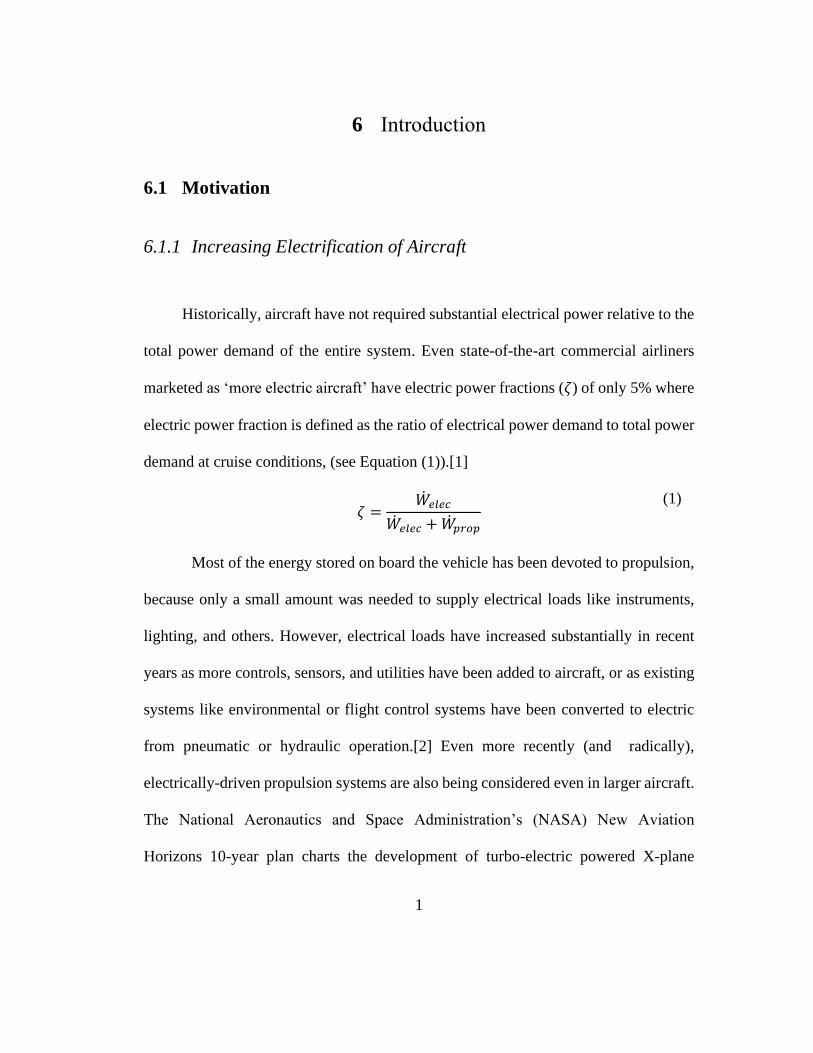
Figure 1 below, reproduced from [4], illustrates this trend, showing differences
in electric power fraction between vehicles, using available data on a range of
aircraft.[5], [6]
Figure 1: Electric Power Fraction at time of First Flight for various aircraft
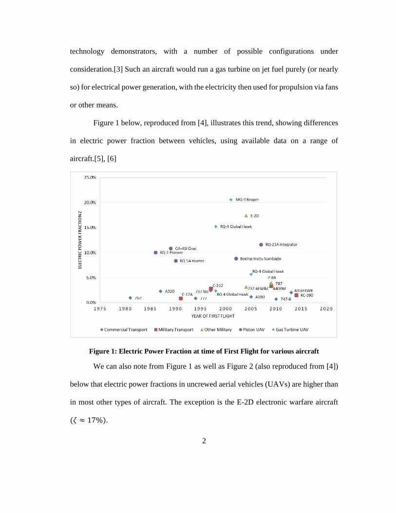
We can also note from Figure 1 as well as Figure 2 (also reproduced from [4])
below that electric power fractions in uncrewed aerial vehicles (UAVs) are higher than
in most other types of aircraft. The exception is the E-2D electronic warfare aircraft
(𝜁 ≈ 17%).
3
Additionally, UAVs are often equipped with advanced sensor packages with
large electrical power demands relative to their size. As a result, 𝜁 can be as large as
21% in the aircraft considered.
In absolute terms, these are not an insubstantial power demands. The MQ-9
Reaper (𝜁 ≈ 21%) requires 49kW of electrical power generation. Even though the
electrical power fraction of the Boeing 787 is only 3.8%, the large scale of the aircraft
implies that a full megawatt of electricity is required.[5], [6] Finally, all-electric aircraft
have been proposed for a variety of purposes, including more efficient fuel usage, as
well as reductions in noise and emissions. The primary challenge is achieving
sufficiently high power to weight ratios for the overall system to be competitive with
turbine engines.[7] Increasing electric power demands also increase the impact of
Figure 2: Estimated electric power fractions in various commercial, military, and unmanned
aircraft.

4
electrical generation efficiency on fuel burn, and thus the range/endurance of the
vehicle.
6.1.2 Existing Electricity Sources and Alternatives
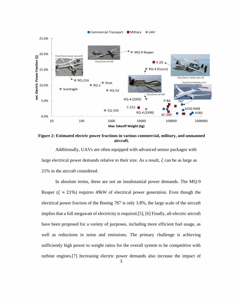
Currently, the most common sources of electrical power on aircraft are shaft-
driven generators (sometimes described as Integrated Drive Generators, or IDGs)
attached as a parasitic loads on the rotating components of the main propulsion system
(see Figure 3) or separate auxiliary power units (APUs).[5], [6]
5
Figure 3: (Top) Schematic of turbofan with Accessory Gearbox and connections
highlighted; (Bottom) Accessories gearbox. including IDG for electricity generation.
Reproduced from [8, pp. 156–157]
Since the electrical generator itself is usually relatively efficient (mechanical to
electrical conversion efficiencies of up to 95% are achievable in many settings[9]), the
overall efficiency is most constrained by the efficiency of the heat engine used to rotate
the generator’s shaft. The underlying thermodynamic cycle is the Otto cycle for a piston
6
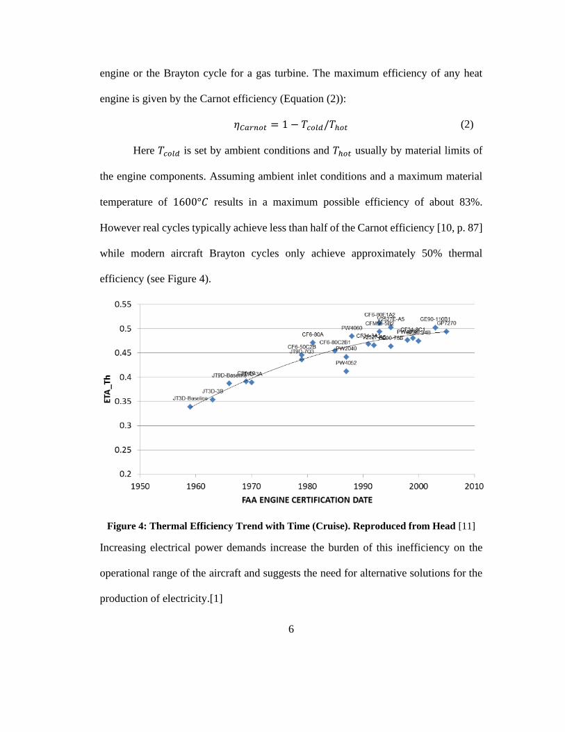
engine or the Brayton cycle for a gas turbine. The maximum efficiency of any heat
engine is given by the Carnot efficiency (Equation (2)):
𝜂𝐶𝑎𝑟𝑛𝑜𝑡 = 1 − 𝑇𝑐𝑜𝑙𝑑/𝑇ℎ𝑜𝑡 (2)
Here 𝑇𝑐𝑜𝑙𝑑 is set by ambient conditions and 𝑇ℎ𝑜𝑡 usually by material limits of
the engine components. Assuming ambient inlet conditions and a maximum material
temperature of 1600°𝐶 results in a maximum possible efficiency of about 83%.
However real cycles typically achieve less than half of the Carnot efficiency [10, p. 87]
while modern aircraft Brayton cycles only achieve approximately 50% thermal
efficiency (see Figure 4).
Figure 4: Thermal Efficiency Trend with Time (Cruise). Reproduced from Head [11]
Increasing electrical power demands increase the burden of this inefficiency on the
operational range of the aircraft and suggests the need for alternative solutions for the
production of electricity.[1]
7
Barring a shaft-driven electrical generator, there are several theoretical sources
for electrical power. Conceivably, nuclear-electric and solar-electric power are options,
but while both have been either considered or executed in a limited sense, nuclear
demands too many risks (or outright pollution) and solar power is not power-dense
enough nor reliably available enough (i.e. cloudy or night-time conditions) for use in
most aircraft applications.[12]
The specific energy of current batteries (100-150 Wh/kg),[13], [14] and
supercapacitors (approximately 1-10 Wh/kg)[15] are so low compared to liquid
hydrocarbon fuels (12.3 kWh/kg) that batteries will consume most if not all of the
aircraft’s useful load capacity. Worse, a battery’s mass does not decrease during flight,
resulting in a further disadvantage compared to liquid fuels. The impact of expending
fuel during flight can be illustrated by comparing the expression for the range of a
fueled aircraft (Equation (3), from Eqn. 5.19 in [16, p. 152]) to the one for a battery-
powered aircraft (Equation (4), derived from integration of Eqn. 5.16 in [16, p. 152]).
𝑠𝑓𝑢𝑒𝑙 = 𝜂0 (
𝐿
𝒟) ln (
𝑚1𝑚2)𝑄𝑅𝑔
(3)
𝑠𝑒𝑙𝑒𝑐 = 𝜂0 (
𝐿
𝒟) (1 −
𝑚2𝑚1)𝑄𝑅𝑔
(4)
Here, 𝑠 is the operating range of the vehicle, 𝑄𝑅 is the specific energy of the
fuel (energy per unit of mass), 𝐿/𝒟 is the vehicle lift to drag ratio, 𝑔 is the acceleration
due to gravity, 𝑚1 is the mass of the aircraft with the power source (fuel or battery)
and 𝑚2 is the empty weight of the aircraft without fuel or battery—equivalent in the
fuel-laden case to be the final mass of the aircraft.[16] For otherwise identical aircraft
8
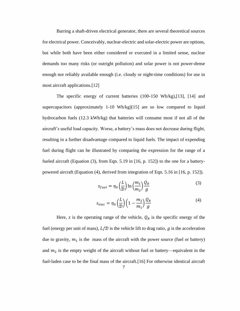
(equivalent propulsive efficiency, 𝐿/𝒟, and empty weight), a fuel-powered aircraft
with 30% fuel mass fraction will have almost 20% greater range than the battery-
powered one simply because the weight of the fuel-powered aircraft decreases over the
course of the flight. Figure 5 below shows that this effect becomes even more important
as the fuel mass fraction increases. For context, an ERJ-145 regional transport jet has
a fuel mass fraction of ~20% (~12% range improvement for fuel over battery) while
the long-haul A380 has a fuel mass fraction of just under 51% (~41% range
improvement).[5]
Figure 5: Percentage Range improvement from expending fuel vs. a retained power
source (e.g. a battery) for a range of fuel/power-source mass fractions
As such, there is substantial advantage to continuing the use of fuel as the
energy source for aircraft with increasingly large electric power requirements.
9
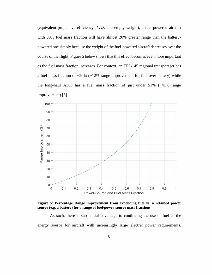
Improvements in this case need to come from the efficiency by which that fuel is
converted to electrical power. As an illustration, we can analyze this scenario as two
separate cycles operating in tandem, as in Figure 6. This is essentially describing an
APU that is more efficient than the main engine.
Figure 6: A single fuel cycle that produces electricity in addition to thrust (top) vs. a
separated cycle with electricity produced with its own fuel supply
To give some idea of what impacts this might have on fuel demand and range,
consider a simple model of the fuel flow rate demand for an aircraft based on the
derivation of the Breguet range equation by Hill and Peterson[16, p. 152] in Equation
(5) where �̇�𝑓 is the fuel flow rate, 𝑚 is the mass of the aircraft, 𝑢 is the aircraft velocity,
𝑄𝑅 is the fuel energy, (𝐿/𝐷) is the lift-to-drag ratio of the airframe and 𝜂𝑜 is the overall
efficiency of the propulsion system:
10
�̇�𝑓 =𝑚𝑔𝑢
𝜂𝑜𝑄𝑅(𝐿/𝐷) (5)
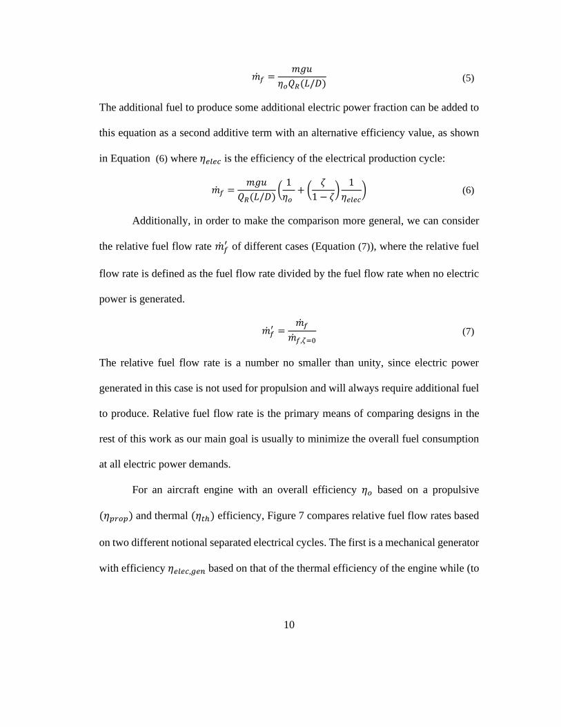
The additional fuel to produce some additional electric power fraction can be added to
this equation as a second additive term with an alternative efficiency value, as shown
in Equation (6) where 𝜂𝑒𝑙𝑒𝑐 is the efficiency of the electrical production cycle:
�̇�𝑓 =
𝑚𝑔𝑢
𝑄𝑅(𝐿/𝐷)(1
𝜂𝑜 + (
𝜁
1 − 𝜁)1
𝜂𝑒𝑙𝑒𝑐) (6)
Additionally, in order to make the comparison more general, we can consider
the relative fuel flow rate �̇�𝑓′ of different cases (Equation (7)), where the relative fuel
flow rate is defined as the fuel flow rate divided by the fuel flow rate when no electric
power is generated.
�̇�𝑓′ =
�̇�𝑓
�̇�𝑓,𝜁=0 (7)
The relative fuel flow rate is a number no smaller than unity, since electric power
generated in this case is not used for propulsion and will always require additional fuel
to produce. Relative fuel flow rate is the primary means of comparing designs in the
rest of this work as our main goal is usually to minimize the overall fuel consumption
at all electric power demands.
For an aircraft engine with an overall efficiency 𝜂𝑜 based on a propulsive
(𝜂𝑝𝑟𝑜𝑝) and thermal (𝜂𝑡ℎ) efficiency, Figure 7 compares relative fuel flow rates based
on two different notional separated electrical cycles. The first is a mechanical generator
with efficiency 𝜂𝑒𝑙𝑒𝑐,𝑔𝑒𝑛 based on that of the thermal efficiency of the engine while (to
11
avoid burying the lede) the second is a fuel cell with a somewhat better efficiency
𝜂𝑒𝑙𝑒𝑐,𝐹𝐶, though the analysis applies to any alternative cycle:
Figure 7: Relative Fuel Flow Rate for Mechanical Generator and Fuel Cell separated
cycles at varying electric power fraction
The numbers provided for efficiency are mainly for illustration, but are
reasonable for aircraft engines[11] and solid oxide fuel cells[10, p. 478]. The results
show an improvement of about 10% in relative fuel flow rate at an electric power
fraction of 25%. This simple analysis does not consider any of the actual properties of
fuel cell operation, so the next section will explore their potential further.
Variable Value
𝜂𝑡h 0.5
𝜂𝑝rop 0.8
𝜂𝐹𝐶 0.6
𝜂𝑔𝑒𝑛 0.95
𝜂𝑜 𝜂𝑡ℎ𝜂𝑝
𝜂𝑒𝑙𝑒𝑐,𝑔𝑒𝑛 𝜂𝑡ℎ𝜂𝑔𝑒𝑛
𝜂𝑒𝑙𝑒𝑐,𝐹𝐶 𝜂𝐹𝐶

12
6.1.3 Potential Solution: Fuel Cells
If we want to retain the advantage of using fuel and rely on the existing aircraft
fuel infrastructure used for most aircraft today, carbon tolerant fuel cells (in particular,
solid-oxide fuel cells or SOFC’s) are an option. Fuel cells are often capable of
producing electrical power from fuel with substantially greater efficiency than heat
engines driving mechanical generators. The potential of this advantage stems from the
different trend in efficiency observed for fuel cells, which is related to the Gibbs Free
Energy rather than the ratio of operating temperatures.
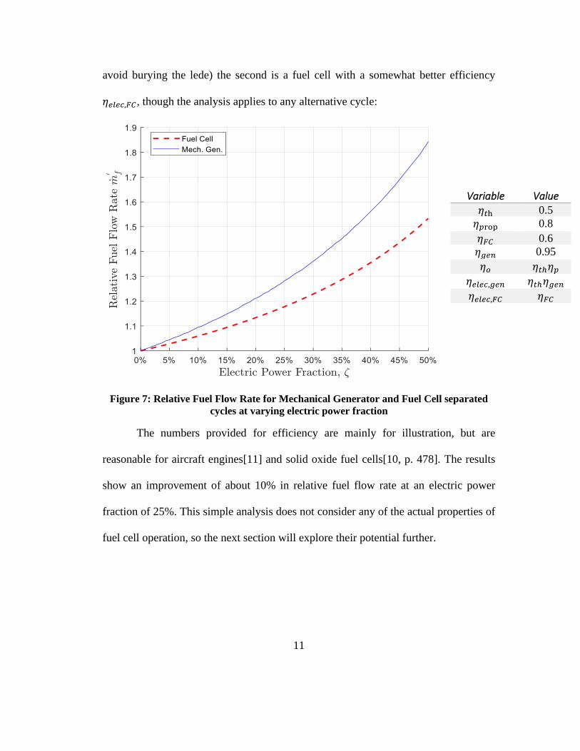
Figure 8 illustrates the comparison while indicating usual operating ranges for
gas turbines and SOFCs. The ideal operating range of the SOFC lies between ambient
conditions, and the maximum required for efficient operation of a large heat engine,
suggesting that those conditions are achievable in the same system.
13
Figure 8: Efficiency Trend with Operating Temperature of Fuel Cells and Brayton Cycle
One important problem with fuel cells is that the infrastructure required to
operate them (pumps, blowers, etc.) can be large and heavy. The problem is
compounded by the need for large fuel cells in order to maximize the conversion of the
fuel to electricity within the cell to avoid simply releasing unburned fuel. These factors
tend to make fuel cell systems inappropriate for use on aircraft in the form of the APU
(i.e. as a separated cycle) previously analyzed. However, recent work has shown that
these problems can be mitigated by integrating the fuel reformer and fuel cell stack
directly into an aircraft gas turbine’s flow path.[17] Next we will expand on this
hybridization of gas turbine and fuel cell.
14
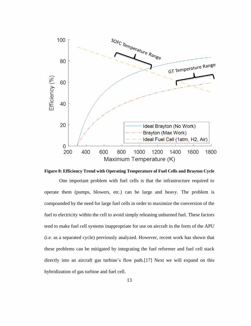
6.1.4 GT-SOFC Hybridization
Explanations of the fundamental operations of gas turbines and fuel cells are
provided in Appendices in sections 13.1 and 13.2 for the reader who is not already
familiar with these technologies. Engine/fuel-cell hybrids come in a variety of forms.
In the case considered here, a solid oxide fuel cell subsystem is inserted into the gas
turbine’s hot section in parallel with the combustor as illustrated in Figure 9. The
reformer, a catalytic partial oxidation reactor (or CPOx) upstream of the fuel cell stack
and the fuel cell stack itself receive pressurized air from the compressor and discharge
their exhaust into the engine’s combustor, enabling any unconsumed fuel to be
recovered in the Brayton cycle.
Figure 9: Simplified layout of turbojet GT-SOFC
15
The advantage of generating electrical power in this way arises from several
possible synergies between the engine and fuel cell:
First, the GT provides most balance of plant functions for the fuel cell stack by
acting as blowers and pumps, as well as providing waste heat that can be used to
maintain the SOFC’s membrane electrode assembly (MEA) at the appropriate
temperature.
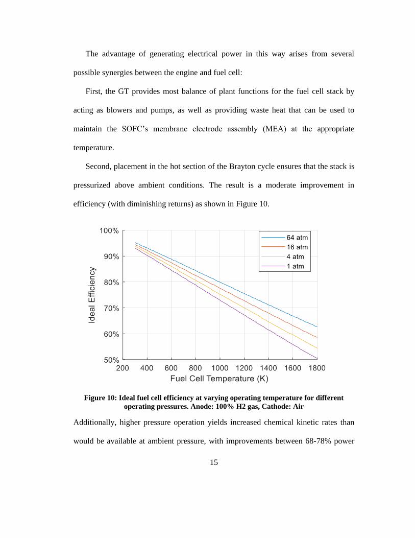
Second, placement in the hot section of the Brayton cycle ensures that the stack is
pressurized above ambient conditions. The result is a moderate improvement in
efficiency (with diminishing returns) as shown in Figure 10.
Figure 10: Ideal fuel cell efficiency at varying operating temperature for different
operating pressures. Anode: 100% H2 gas, Cathode: Air
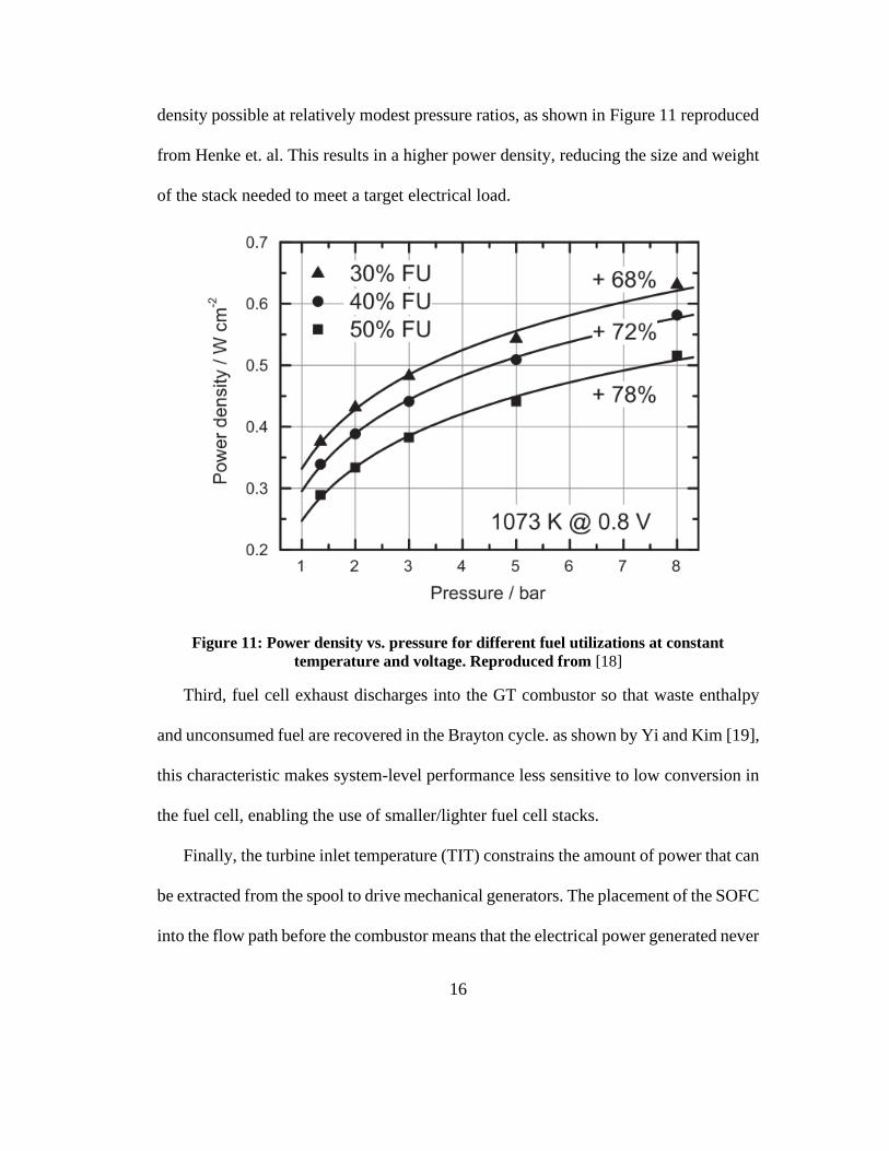
Additionally, higher pressure operation yields increased chemical kinetic rates than
would be available at ambient pressure, with improvements between 68-78% power
16
density possible at relatively modest pressure ratios, as shown in Figure 11 reproduced
from Henke et. al. This results in a higher power density, reducing the size and weight
of the stack needed to meet a target electrical load.
Figure 11: Power density vs. pressure for different fuel utilizations at constant
temperature and voltage. Reproduced from [18]
Third, fuel cell exhaust discharges into the GT combustor so that waste enthalpy
and unconsumed fuel are recovered in the Brayton cycle. as shown by Yi and Kim [19],
this characteristic makes system-level performance less sensitive to low conversion in
the fuel cell, enabling the use of smaller/lighter fuel cell stacks.
Finally, the turbine inlet temperature (TIT) constrains the amount of power that can
be extracted from the spool to drive mechanical generators. The placement of the SOFC
into the flow path before the combustor means that the electrical power generated never
17
reaches the turbine as additional heat, only the waste enthalpy from SOFC
inefficiencies. The result is that greater amounts of electrical power can be generated
before encountering the TIT material limitations.
6.2 Prior Work
6.2.1 GT/SOFC Literature Review
Waters reviewed the literature in 2015 and identified a range of research on
ground-based hybridized GT-SOFC power plants, GT-SOFC APUs for aircraft, and
all-electric UAVs and compared the scale, efficiency, fuel, and other characteristics of
the various systems.[1], [17] Most of the studies of hybridization focus on integrated
GT-SOFC systems for large-scale stationary ground-based power generation rather
than aircraft [20]–[28]. At least one hybrid system used a molten carbonate fuel cell
(MCFC) [29]. Natural gas [20], [23], [26] methane [21], [24], [25], [29] and syngas
[27], [28] are the fuels considered. Both external[24]–[27] and internal[20]–[23] fuel
reformers are employed with powers ranging from 5 kilowatts[26] to 2.4
megawatts[21]. A separate review of GT-SOFC hybridization in power plant
applications reaffirmed the efficiency and fuel flexibility advantages offered by
hybridization.[30] Another review article discussed transient operation and controls for
hybrid power plants.[31]
One notable takeaway from the range of work described above is that most
studies, especially those for vehicles, use very simplistic fuel cell models that do not

18
account for ‘down the channel’ performance. Also, of the already small number of
studies focused on aircraft, even fewer consider traditional hydrocarbon fuels and use
for combined propulsion and power.
An updated survey of the literature since Waters’ 2015 review includes
additional GT-SOFC power plant models in several different configurations. An
interesting general finding that applies to this work was found by Yi and Kim; that
the optimal SOFC conversion rate for hybrid systems such as GT-SOFCs drops
substantially compared to standalone SOFC systems—in their scenarios to 70% from
80% in a ground-based system.[19] Almost all works found use simple (i.e. zero-
dimensional) fuel cell models although some are at least validated via comparison to
existing systems.[19], [32]–[35] Modeling has been performed in MATLAB,[36]
Aspen HYSIS,[19], [37] custom iterative solvers,[35], [38], [39] or even
optimizations through a genetic algorithm[34]. An exception is a power plant study
by Dang, Zhao, and Xi however noted deficiencies (in particular problematic
temperature distributions inside the cell) in black-box or zero-dimensional models,
and attempt to reach higher fidelity through what they describe as a “quasi-2D
model.”[40]
Regarding aircraft hybrid systems, Valencia et. al. provide a distributed
electrical fan system along with a turbofan for propulsion driven by a hybrid GT-
SOFC system using liquid hydrogen for the fuel cell and kerosene for the GT. They
employ another zero-dimensional SOFC model but include mass modeling
considerations for the fuel cell and hydrogen storage, and use a similar notional

19
SOFC location to this work.[41] A more complicated one-dimensional Simulink
model developed by Chakravarthula, Roberts, and Wolff uses an internal steam
reformer in an SOFC-combustor model, requiring the combustor to initially heat air
entering the SOFC.[42] The intended system configuration uses an electrically-driven
compressor (powered by the SOFC as the only load), removing the need for a turbine
before passing the hot exhaust gases through a nozzle to produce thrust. However,
their SOFC model applies a very limited set of reactions possible at anode and
cathode, makes modeling assumptions including no variation in temperature for cells
at the edge of a stack versus the center, and neglects pressure losses through the
SOFC. Furthermore, at this point in development the overall system described does
not account for the water required in order to operate the steam reformer. Similarly
employing the electric power from the SOFC for propulsion, Okai et. al. use another
Simulink model to investigate a “core” GT-SOFC hybrid power generator that
provides propulsive thrust as well as electrical power provided to other fans dedicated
to boundary-layer ingestion.[43]–[45] They also use what is likely a zero-dimensional
model but the precise methodology is not well specified although it is claimed that the
model accounts for stack size “Partial pressure, thermal relations, losses, and other
points.”[43]
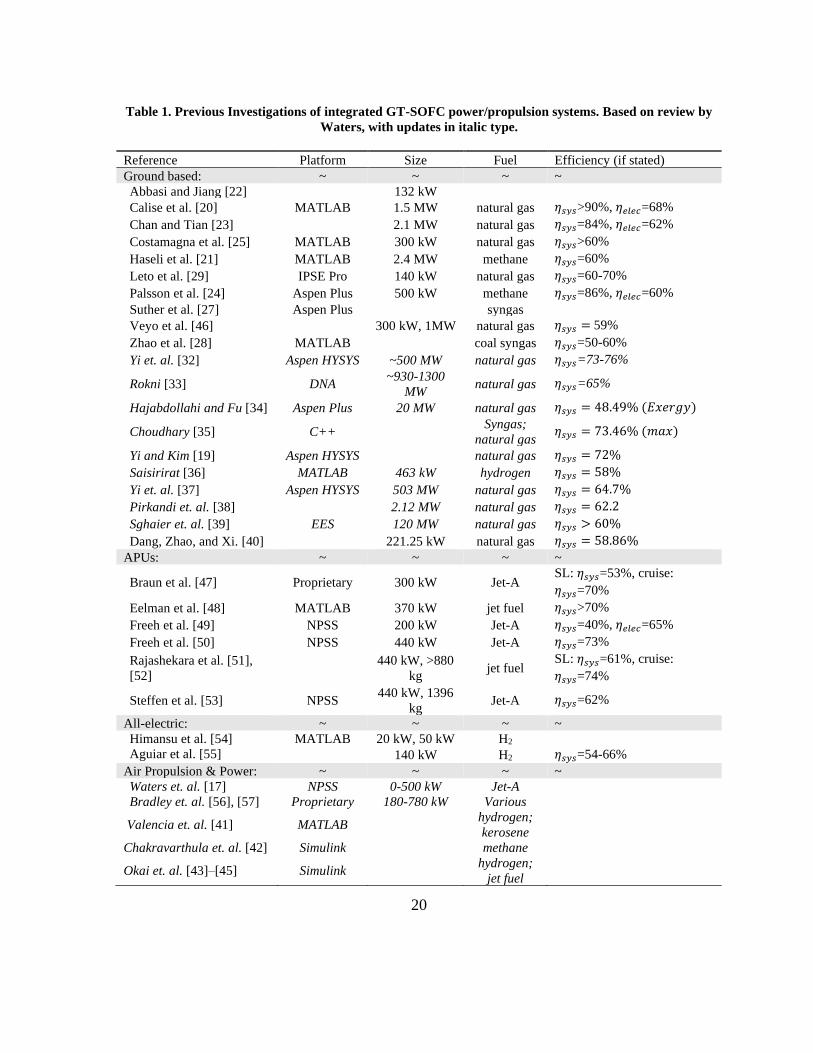
An extended version of the literature summary table initially developed by
Waters [17] is included as Table 1 below.
20
Table 1. Previous Investigations of integrated GT-SOFC power/propulsion systems. Based on review by
Waters, with updates in italic type.
Reference Platform Size Fuel Efficiency (if stated)
Ground based: ~ ~ ~ ~
Abbasi and Jiang [22] 132 kW
Calise et al. [20] MATLAB 1.5 MW natural gas 𝜂𝑠𝑦𝑠>90%, 𝜂𝑒𝑙𝑒𝑐=68%
Chan and Tian [23] 2.1 MW natural gas 𝜂𝑠𝑦𝑠=84%, 𝜂𝑒𝑙𝑒𝑐=62%
Costamagna et al. [25] MATLAB 300 kW natural gas 𝜂𝑠𝑦𝑠>60%
Haseli et al. [21] MATLAB 2.4 MW methane 𝜂𝑠𝑦𝑠=60%
Leto et al. [29] IPSE Pro 140 kW natural gas 𝜂𝑠𝑦𝑠=60-70%
Palsson et al. [24] Aspen Plus 500 kW methane 𝜂𝑠𝑦𝑠=86%, 𝜂𝑒𝑙𝑒𝑐=60%
Suther et al. [27] Aspen Plus syngas
Veyo et al. [46] 300 kW, 1MW natural gas 𝜂𝑠𝑦𝑠 = 59%
Zhao et al. [28] MATLAB coal syngas 𝜂𝑠𝑦𝑠=50-60%
Yi et. al. [32] Aspen HYSYS ~500 MW natural gas 𝜂𝑠𝑦𝑠=73-76%
Rokni [33] DNA ~930-1300
MW natural gas 𝜂𝑠𝑦𝑠=65%
Hajabdollahi and Fu [34] Aspen Plus 20 MW natural gas 𝜂𝑠𝑦𝑠 = 48.49% (𝐸𝑥𝑒𝑟𝑔𝑦)
Choudhary [35] C++ Syngas;
natural gas 𝜂𝑠𝑦𝑠 = 73.46% (𝑚𝑎𝑥)
Yi and Kim [19] Aspen HYSYS natural gas 𝜂𝑠𝑦𝑠 = 72%
Saisirirat [36] MATLAB 463 kW hydrogen 𝜂𝑠𝑦𝑠 = 58%
Yi et. al. [37] Aspen HYSYS 503 MW natural gas 𝜂𝑠𝑦𝑠 = 64.7%
Pirkandi et. al. [38] 2.12 MW natural gas 𝜂𝑠𝑦𝑠 = 62.2
Sghaier et. al. [39] EES 120 MW natural gas 𝜂𝑠𝑦𝑠 > 60%
Dang, Zhao, and Xi. [40] 221.25 kW natural gas 𝜂𝑠𝑦𝑠 = 58.86%
APUs: ~ ~ ~ ~
Braun et al. [47] Proprietary 300 kW Jet-A SL: 𝜂𝑠𝑦𝑠=53%, cruise:
𝜂𝑠𝑦𝑠=70%
Eelman et al. [48] MATLAB 370 kW jet fuel 𝜂𝑠𝑦𝑠>70%
Freeh et al. [49] NPSS 200 kW Jet-A 𝜂𝑠𝑦𝑠=40%, 𝜂𝑒𝑙𝑒𝑐=65%
Freeh et al. [50] NPSS 440 kW Jet-A 𝜂𝑠𝑦𝑠=73%
Rajashekara et al. [51],
[52]
440 kW, >880
kg jet fuel
SL: 𝜂𝑠𝑦𝑠=61%, cruise:
𝜂𝑠𝑦𝑠=74%
Steffen et al. [53] NPSS 440 kW, 1396
kg Jet-A 𝜂𝑠𝑦𝑠=62%
All-electric: ~ ~ ~ ~
Himansu et al. [54] MATLAB 20 kW, 50 kW H2
Aguiar et al. [55] 140 kW H2 𝜂𝑠𝑦𝑠=54-66%
Air Propulsion & Power: ~ ~ ~ ~
Waters et. al. [17] NPSS 0-500 kW Jet-A
Bradley et. al. [56], [57] Proprietary 180-780 kW Various
Valencia et. al. [41] MATLAB hydrogen;
kerosene
Chakravarthula et. al. [42] Simulink methane
Okai et. al. [43]–[45] Simulink hydrogen;
jet fuel
21
Comparing the state of the art today with that identified by Waters in 2015, it
is apparent that the majority of research involving hybrid GT-SOFC systems
continues to use zero-dimensional fuel cell models in both ground power and aircraft-
based systems. The rare exceptions are Dang, Zhao and Xi with their quasi-2D model,
and Chakravarthula, Roberts, and Wolff, who apply a complex quasi-1D SOFC
model, though still with modeling simplifications such as a small number of
electrochemical reactions considered within the flow, and an incomplete set of
turbomachinery components for a complete cycle analysis. Additionally, studies on
fuel-cell-based all-electric or electrically-assisted vehicle propulsion systems tend to
focus on hydrogen gas as a primary fuel for the SOFC, as well as the use of the
electrical power generated by the system to drive fans to produce additional thrust.
6.2.2 Prior Work at Maryland
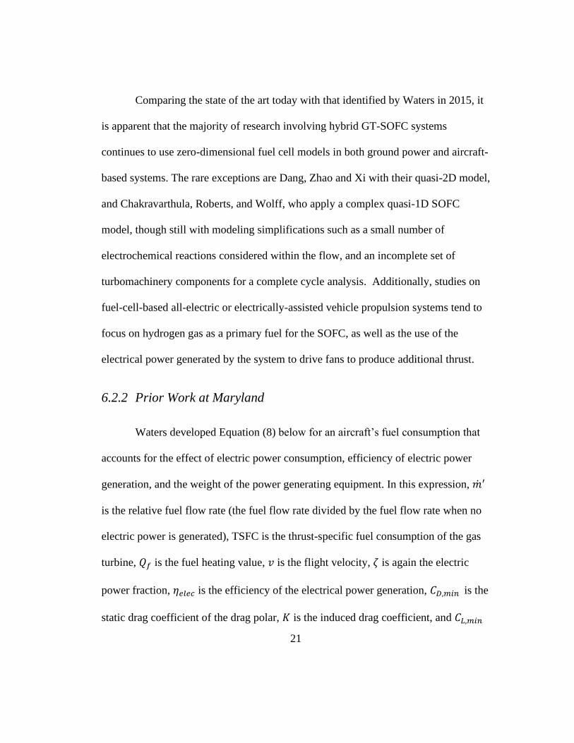
Waters developed Equation (8) below for an aircraft’s fuel consumption that
accounts for the effect of electric power consumption, efficiency of electric power
generation, and the weight of the power generating equipment. In this expression, �̇�′
is the relative fuel flow rate (the fuel flow rate divided by the fuel flow rate when no
electric power is generated), TSFC is the thrust-specific fuel consumption of the gas
turbine, 𝑄𝑓 is the fuel heating value, 𝑣 is the flight velocity, 𝜁 is again the electric
power fraction, 𝜂𝑒𝑙𝑒𝑐 is the efficiency of the electrical power generation, 𝐶𝐷,𝑚𝑖𝑛 is the
static drag coefficient of the drag polar, 𝐾 is the induced drag coefficient, and 𝐶𝐿,𝑚𝑖𝑛
22
is the lift coefficient, 𝑚0 and 𝑚𝑒𝑙𝑒𝑐 are initial masses and the varying mass of the
electrical generating system respectively, 𝑆 is the aircraft wing area, 𝑔 is the
acceleration due to gravity, and 𝜌 is the air density:[1]
�̇�𝑓′ = (1 +
𝜈
(𝑇𝑆𝐹𝐶)𝑄𝑅𝜂𝑒𝑙𝑒𝑐[𝜁
1 − 𝜁])
[𝐶𝐷,𝑚𝑖𝑛 + 𝐾((𝑚0 +𝑚𝑒𝑙𝑒𝑐)𝑔
12𝜌𝜈2𝑆
− 𝐶𝐿,𝑚𝑖𝑛 )
2
]
[𝐶𝐷,𝑚𝑖𝑛 + 𝐾(𝑚0𝑔12𝜌𝜈2𝑆
− 𝐶𝐿,𝑚𝑖𝑛 )
2
]
(8)
Equation (8) shows that increasing the electric power fraction increases fuel
consumption which in turn decreases range and endurance. It also shows that the
sensitivity of fuel flow rate to electrical generator weight depends on the induced drag
coefficient (𝐾) of the vehicle and weight of the generator relative to the vehicle’s
empty weight. Thus, the additional weight of the fuel cell influences the overall fuel
consumption rate of the vehicle.
The propulsion system (and vehicle performance) were modeled using a
NASA-developed simulation environment called Numerical Propulsion System
Simulation (NPSS).[58] The output of this research was a range of integrated gas
turbine and solid-oxide fuel cell (GT-SOFC) system models that included, most
notably, a set of fuel cell component models that were much more advanced than
those used in most (if not all) prior hybrid modeling efforts. These advanced features
included down-the-channel performance variation, multi-step equilibrium chemistry,
realistic representations of heat transfer within the fuel cell structure, and realistic
23
representation of oxygen ion transport via the dusty gas model [59] through the
electrolyte. Some key conclusions of Waters’ work were:
• GT-SOFC hybridization can reduce fuel consumption in Global-Hawk class
UAVs by 5% or more depending upon how much electric power is desired.
• GT-SOFC hybridization can produce more than five times the amount of
electric power than a spool-driven mechanical generator before encountering
the turbine inlet temperature limitation of the engine.
• External aerodynamic drag could be an important limitation in pylon-mounted
applications.
The promise of GT-SOFC hybridization identified by Waters led to follow-on
efforts to construct and test a bench-scale prototype of a GT-SOFC hybrid that could
be used to validate system models and to identify practical problems associated with
integrating solid oxide fuel cells into the hot section of a gas turbine. Since the main
goal is learning – not to produce a ‘practical’ flight weight system at this stage – it
was decided to construct one using commercial off-the-shelf (COTS) engines and fuel
cells. A small turbojet engine (AMT Olympus HP) was selected for this purpose and
characterized by Vannoy who measured its performance and developed a validated
model of the engine in NPSS [4], [60]–[62].

24
6.3 Objective and Approach
6.3.1 Objectives
The objectives pursued by this thesis are threefold. The first objective is to
improve the features of the GT-SOFC model by investigating the effects of flow path
and aerodynamic drag on overall fuel consumption in pylon-mounted configurations.
The second objective is to develop an experimentally validated model of a COTS fuel
cell (an Adaptive Materials Defender D300 [63]). Finally, the GT-SOFC model will
be scaled down to the general size of the COTS fuel cell and coupled with Vannoy’s
model of a COTS gas turbine (an AMT Olympus High Power) to provide general
sizing information for a system model that can inform the design of an integrated
bench-scale demonstrator based on these components. Future work will integrate the
COTS fuel cell model to improve the design on the bench-scale generator. Taken
together, the overall objective of the thesis is to improve our understanding of how to
exploit GT-SOFC hybridization to reduce fuel consumption in aircraft.
6.3.2 Approach
The overall approach in this work has three main steps. First, I investigate the
effects of external aerodynamic drag on vehicle-level fuel consumption in the larger
pylon-mounted configurations that Waters investigated. Second, I measure the
performance and physical characteristics of the COTS APU looking towards using
this information to develop an experimentally validated model of the integrated
25
CPOx/SOFC components in NPSS. Finally, I scale down and integrate the
CPOx/SOFC model with Vannoy’s GT model and use the resulting system model to
predict the operating characteristics (temperatures, flow rates, etc.) needed in order to
design the bench-scale prototype. Future measurements of APU performance will be
used to improve this initial system model.
6.3.3 COTS Components
The bench-scale GT platform considered in this modeling effort is the AMT
Olympus High Power, a small 230N of thrust kerosene-fueled turbojet. The inflow
rate for the engine is 0.45 kg/s at maximum thrust, with a corresponding maximum
RPM of 108,500. The engine was acquired in ‘university configuration’ which means
that it has pre-installed ports for measuring temperatures and pressures at the various
internal stages of the gas turbine cycle.
The APU is an Adaptive Materials Defender D300, capable of generating a
maximum of 300 Watts of electrical power.[63] It is rated at 32V and 9.5 Amps
maximum output. The system is fueled by propane at approximately 1 standard cubic
centimeter per second fed through a sulfur filter. The system is started by a lithium
ion battery that maintains the balance of plant as the SOFC reaches its operating
temperature.
Figure 12 below shows both COTS systems side by side (the engine is on a
thrust stand) to provide a sense of relative scale.
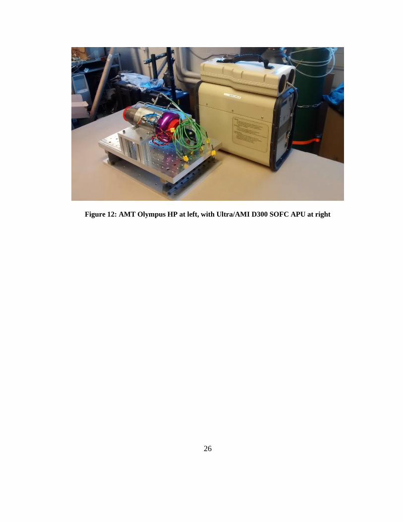
26
Figure 12: AMT Olympus HP at left, with Ultra/AMI D300 SOFC APU at right

27
7 Modeling Environment
7.1 Overview
7.1.1 Background
NPSS[58], [64]–[67] is a gas turbine modeling code and framework
developed by NASA with the intention of being highly customizable in both
complexity and scope. It is further designed to be able to include a variety of custom
components that can function as “black boxes” in order to enable consortia of engine
manufacturing companies to collaborate without revealing proprietary information.
From a practical perspective, the modeling language is object-oriented, and closely
based on C++. NPSS was also the simulation platform used in the work immediately
preceding this thesis. [1], [17], [68]
An engine is modeled in NPSS by linking together models of individual
engine components like compressors, combustors, fans, ducts, turbines, and nozzles.
These component models are also often referred to as “elements”. The elements
usually contain dependent and independent variables. NPSS solves the system by
adjusting the values of the independent variables in order to conserve mass and
energy while maintaining any other conditions specified for each component. The
number of independent variables must equal the number of dependent variables in
order to have a solvable system.

28
7.1.2 Solver Process
The component files and list of connections are considered the “model” of a
specific system under consideration. Additionally, other files may be called or
included to perform calculations or collect data. Finally, a case (file) is specified,
which provides specific operating conditions and a range of dependent and
independent variables to solve for the given case.
The solution process for any given case assumes a number of “dependent”
characteristics, variables for which the system is required to match, as well as an
equal number of “independent” values that may be altered in order to yield the
dependent values. Another way of thinking about this is that there are a number of
targets we want to achieve (for instance a particular turbine inlet temperature), and an
equal number of knobs (for instance, the fuel flow rate into a combustor) to turn in
order to reach these targets. Engine size parameters can also be independent variables
meaning that the engine can be essentially “rubber” if need be. Given a set of starting
conditions, the solver uses a modified Newton’s method with Broyden updates to
drive the values of the dependent variables to their intended targets by adjusting the
values of the independent parameters.[69] This is accomplished by calculating a
Jacobian matrix that contains the first derivatives of each independent variable with
respect to each dependent variable. Calculating the Jacobian is computationally
expensive so the inexact Broyden update method (generating an approximation of the
29
Jacobian by comparison to the previous iteration of the calculation) is often used until
certain solution criteria are not met.[69]
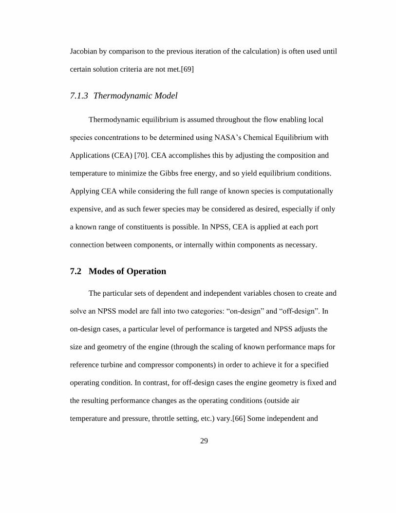
7.1.3 Thermodynamic Model
Thermodynamic equilibrium is assumed throughout the flow enabling local
species concentrations to be determined using NASA’s Chemical Equilibrium with
Applications (CEA) [70]. CEA accomplishes this by adjusting the composition and
temperature to minimize the Gibbs free energy, and so yield equilibrium conditions.
Applying CEA while considering the full range of known species is computationally
expensive, and as such fewer species may be considered as desired, especially if only
a known range of constituents is possible. In NPSS, CEA is applied at each port
connection between components, or internally within components as necessary.
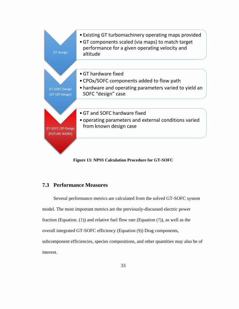
7.2 Modes of Operation
The particular sets of dependent and independent variables chosen to create and
solve an NPSS model are fall into two categories: “on-design” and “off-design”. In
on-design cases, a particular level of performance is targeted and NPSS adjusts the
size and geometry of the engine (through the scaling of known performance maps for
reference turbine and compressor components) in order to achieve it for a specified
operating condition. In contrast, for off-design cases the engine geometry is fixed and
the resulting performance changes as the operating conditions (outside air
temperature and pressure, throttle setting, etc.) vary.[66] Some independent and
30
dependent variables are the same in both modes of operation. Examples include the
requirement for steady-state operation that the net torque on all spool shafts is zero,
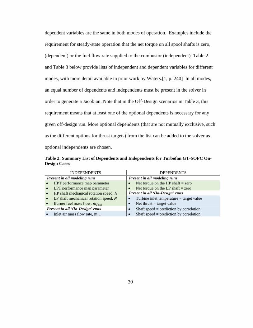
(dependent) or the fuel flow rate supplied to the combustor (independent). Table 2
and Table 3 below provide lists of independent and dependent variables for different
modes, with more detail available in prior work by Waters.[1, p. 240] In all modes,
an equal number of dependents and independents must be present in the solver in
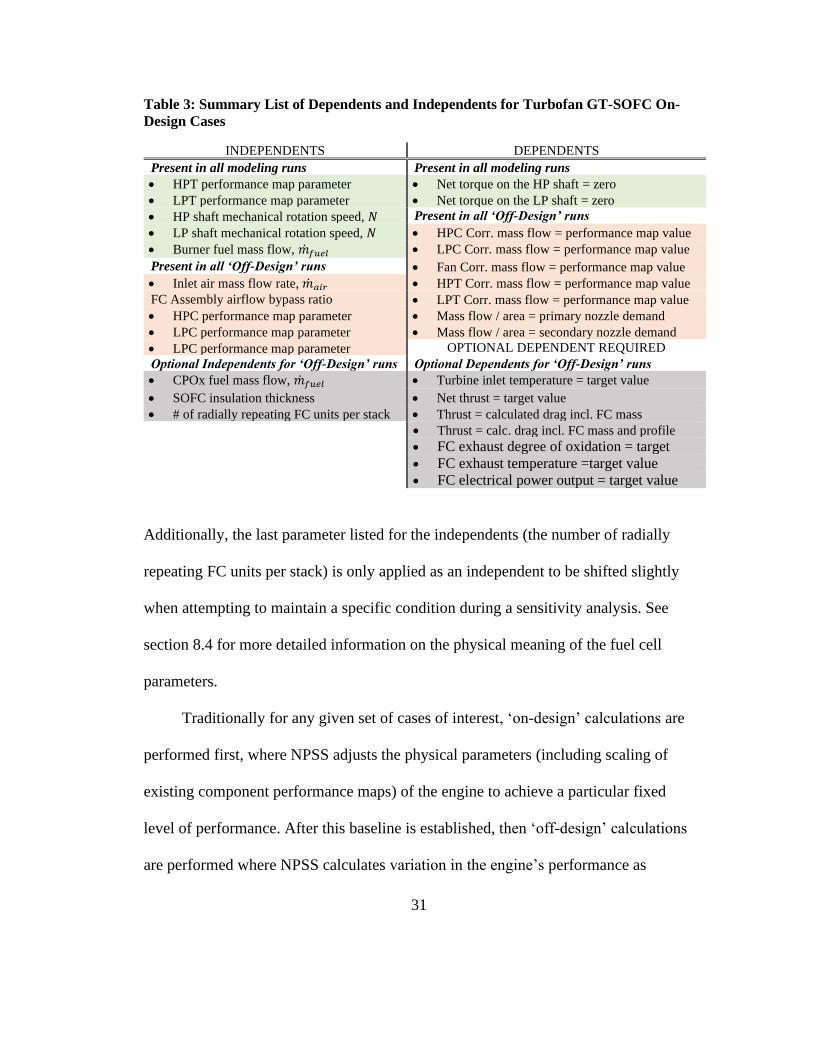
order to generate a Jacobian. Note that in the Off-Design scenarios in Table 3, this
requirement means that at least one of the optional dependents is necessary for any
given off-design run. More optional dependents (that are not mutually exclusive, such
as the different options for thrust targets) from the list can be added to the solver as
optional independents are chosen.
Table 2: Summary List of Dependents and Independents for Turbofan GT-SOFC On-
Design Cases
INDEPENDENTS DEPENDENTS
Present in all modeling runs Present in all modeling runs
• HPT performance map parameter • Net torque on the HP shaft = zero
• LPT performance map parameter • Net torque on the LP shaft = zero
• HP shaft mechanical rotation speed, 𝑁 Present in all ‘On-Design’ runs
• LP shaft mechanical rotation speed, 𝑁 • Turbine inlet temperature = target value
• Burner fuel mass flow, �̇�𝑓𝑢𝑒𝑙 • Net thrust = target value
Present in all ‘On-Design’ runs • Shaft speed = prediction by correlation
• Inlet air mass flow rate, �̇�𝑎𝑖𝑟 • Shaft speed = prediction by correlation
31
Table 3: Summary List of Dependents and Independents for Turbofan GT-SOFC On-
Design Cases
INDEPENDENTS DEPENDENTS
Present in all modeling runs Present in all modeling runs
• HPT performance map parameter • Net torque on the HP shaft = zero
• LPT performance map parameter • Net torque on the LP shaft = zero
• HP shaft mechanical rotation speed, 𝑁 Present in all ‘Off-Design’ runs
• LP shaft mechanical rotation speed, 𝑁 • HPC Corr. mass flow = performance map value
• Burner fuel mass flow, �̇�𝑓𝑢𝑒𝑙 • LPC Corr. mass flow = performance map value
Present in all ‘Off-Design’ runs • Fan Corr. mass flow = performance map value
• Inlet air mass flow rate, �̇�𝑎𝑖𝑟 • HPT Corr. mass flow = performance map value
FC Assembly airflow bypass ratio • LPT Corr. mass flow = performance map value
• HPC performance map parameter • Mass flow / area = primary nozzle demand
• LPC performance map parameter • Mass flow / area = secondary nozzle demand
• LPC performance map parameter OPTIONAL DEPENDENT REQUIRED
Optional Independents for ‘Off-Design’ runs Optional Dependents for ‘Off-Design’ runs
• CPOx fuel mass flow, �̇�𝑓𝑢𝑒𝑙 • Turbine inlet temperature = target value
• SOFC insulation thickness • Net thrust = target value
• # of radially repeating FC units per stack • Thrust = calculated drag incl. FC mass
• Thrust = calc. drag incl. FC mass and profile
• FC exhaust degree of oxidation = target • FC exhaust temperature =target value
• FC electrical power output = target value
Additionally, the last parameter listed for the independents (the number of radially
repeating FC units per stack) is only applied as an independent to be shifted slightly
when attempting to maintain a specific condition during a sensitivity analysis. See
section 8.4 for more detailed information on the physical meaning of the fuel cell
parameters.
Traditionally for any given set of cases of interest, ‘on-design’ calculations are
performed first, where NPSS adjusts the physical parameters (including scaling of
existing component performance maps) of the engine to achieve a particular fixed
level of performance. After this baseline is established, then ‘off-design’ calculations
are performed where NPSS calculates variation in the engine’s performance as

32
operating conditions (like outside air temperature, outside air pressure, throttle
setting, etc.) are adjusted over a range of conditions.
In this work, for all cases the physical characteristics of the engine are first
determined using an ‘on-design’ calculation where no CPOx/SOFC subsystem is
present. Subsequent calculations add the CPOx/SOFC subsystem and operate in ‘off-
design’ mode for the gas turbine components which essentially ‘fixes’ the baseline
gas turbine hardware. Various fuel cell hardware and operating parameters (this
scenario’s ‘independent variables’) are adjusted to meet a set of specified electrical
load and/or targeted internal conditions. By convention of the NPSS software, the
fuel cell components of the GT-SOFC are designed (i.e. their physical parameters
determined) in this ‘off-design’ state in order to fix the design (i.e. sizing) of the
turbomachinery components while the overall GT-SOFC system may be considered
‘on-design’. True ‘off-design’ operation for the full GT-SOFC system is relegated to
future work. Figure 13 illustrates this progression.
33
Figure 13: NPSS Calculation Procedure for GT-SOFC
7.3 Performance Measures
Several performance metrics are calculated from the solved GT-SOFC system
model. The most important metrics are the previously-discussed electric power
fraction (Equation. (1)) and relative fuel flow rate (Equation (7)), as well as the
overall integrated GT-SOFC efficiency (Equation (9)) Drag components,
subcomponent efficiencies, species compositions, and other quantities may also be of
interest.
GT Design
• Existing GT turbomachinery operating maps provided
• GT components scaled (via maps) to match target performance for a given operating velocity and altitude
GT-SOFC Design
(GT Off-Design)
• GT hardware fixed
• CPOx/SOFC components added to flow path
• hardware and operating parameters varied to yield an SOFC “design” case
GT-SOFC Off-Design
[FUTURE WORK]
• GT and SOFC hardware fixed
• operating parameters and external conditions varied from known design case
34
Finally the overall efficiency of the system, (Eqn. (9)) defined as the electrical
plus propulsive power divided by the fuel input power (fuel flow rate times the heat
of combustion), is another performance metric considered.
𝜂𝑜𝑣𝑒𝑟 =
(�̇�𝑝𝑟𝑜𝑝 + �̇�𝑒𝑙𝑒𝑐)
�̇�𝑓𝑄𝑅 (9)
The overall efficiency compares the total useful energy extracted from the fuel
consumed to the total energy available in the fuel via combustion. This value is less
operationally important in aircraft than relative fuel flow rate but is relevant for
general comparison to other hybrid power systems like terrestrial installations where
no vehicle baseline consumption exists.
7.4 Viewers and Analysis Tools
In NPSS, the results of a solution are traditionally output to DataViewer
(hereafter “viewer”) files, which are separate scripts that collect and output data from
the model into useful formats. Prior work by Waters developed customized viewers
for the GT-SOFC model, though these were limited to specific important variables
deemed important at runtime. However, experience has shown that performing further
analysis will often require additional information regarding system state that would
be inaccessible without rerunning the simulation—often costly in terms of time, and
storage of the precise script for a given scenario. As part of this work, a custom NPSS
viewer/function (“SaveAll”) was developed to extend the built-in VarDumpViewer,

35
[66, p. 99] which captures and outputs all existing variables in the computational
model in a list to the terminal.
The custom viewer captures these list outputs for each solution and places them
into a single file. An external script is then used to reorganize the long lists into a
tabular format where each row represents a single NPSS solution. The result is
usually a table with tens of thousands of columns and relatively few (<100) rows.
Data processing software such as MATLAB can effectively pull selected columns
(i.e. variables) from the large table for analysis; interrogating new variables only
requires providing their name and re-reading the large table file. This custom viewer
is general to NPSS and minimizes requirements to make alterations to standard
viewer files to collect and process data as changes and updates are made to
experimental models.
36
8 GT-SOFC System Model
The models discussed in this section are oriented towards the design of a
laboratory-scale demonstrator system. The models used to investigate drag effects
will be explained in Chapter 9. The GT and the SOFC subsystem (comprising of the
CPOx, fuel cell inlet, SOFC, and combiner components) models can be considered
separately prior to integration into a single model. For simplicity, we will consider a
turbojet system in this section, but the same explanations hold for other systems in
this work such as turbofans with the addition of additional compressor and turbine
stages and a fan component.
8.1 Gas Turbine NPSS Model
More detailed information about each of these components is available
elsewhere [1, Ch. 2] but summaries have been included here for convenience.
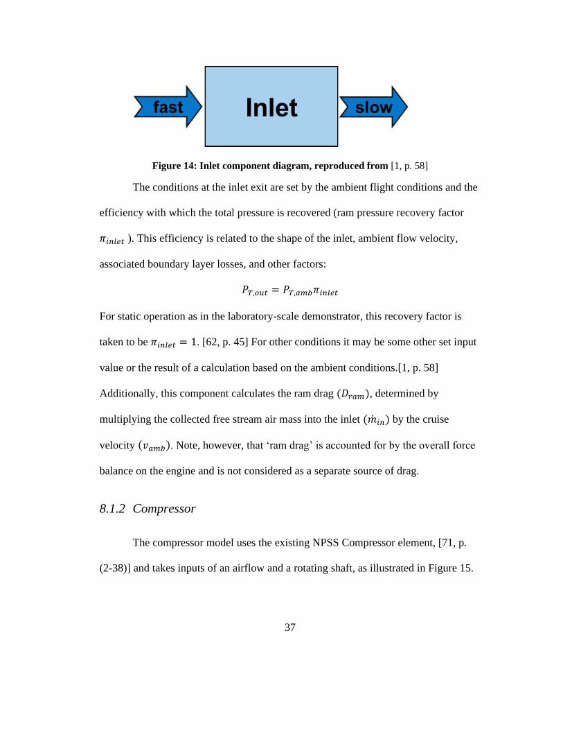
8.1.1 Inlet
The standard NPSS Inlet component [71, p. (2-68)] accepts (and usually
slows) the incoming flow prior to entering the compressor. It is sketched
schematically in Figure 14.
37
Figure 14: Inlet component diagram, reproduced from [1, p. 58]
The conditions at the inlet exit are set by the ambient flight conditions and the
efficiency with which the total pressure is recovered (ram pressure recovery factor
𝜋𝑖𝑛𝑙𝑒𝑡 ). This efficiency is related to the shape of the inlet, ambient flow velocity,
associated boundary layer losses, and other factors:
𝑃𝑇,𝑜𝑢𝑡 = 𝑃𝑇,𝑎𝑚𝑏𝜋𝑖𝑛𝑙𝑒𝑡
For static operation as in the laboratory-scale demonstrator, this recovery factor is
taken to be 𝜋𝑖𝑛𝑙𝑒𝑡 = 1. [62, p. 45] For other conditions it may be some other set input
value or the result of a calculation based on the ambient conditions.[1, p. 58]
Additionally, this component calculates the ram drag (𝐷𝑟𝑎𝑚), determined by
multiplying the collected free stream air mass into the inlet (�̇�𝑖𝑛) by the cruise
velocity (𝑣𝑎𝑚𝑏). Note, however, that ‘ram drag’ is accounted for by the overall force
balance on the engine and is not considered as a separate source of drag.
8.1.2 Compressor
The compressor model uses the existing NPSS Compressor element, [71, p.
(2-38)] and takes inputs of an airflow and a rotating shaft, as illustrated in Figure 15.
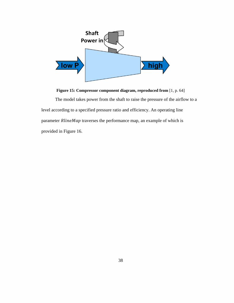
38
Figure 15: Compressor component diagram, reproduced from [1, p. 64]
The model takes power from the shaft to raise the pressure of the airflow to a
level according to a specified pressure ratio and efficiency. An operating line
parameter 𝑅𝑙𝑖𝑛𝑒𝑀𝑎𝑝 traverses the performance map, an example of which is
provided in Figure 16.
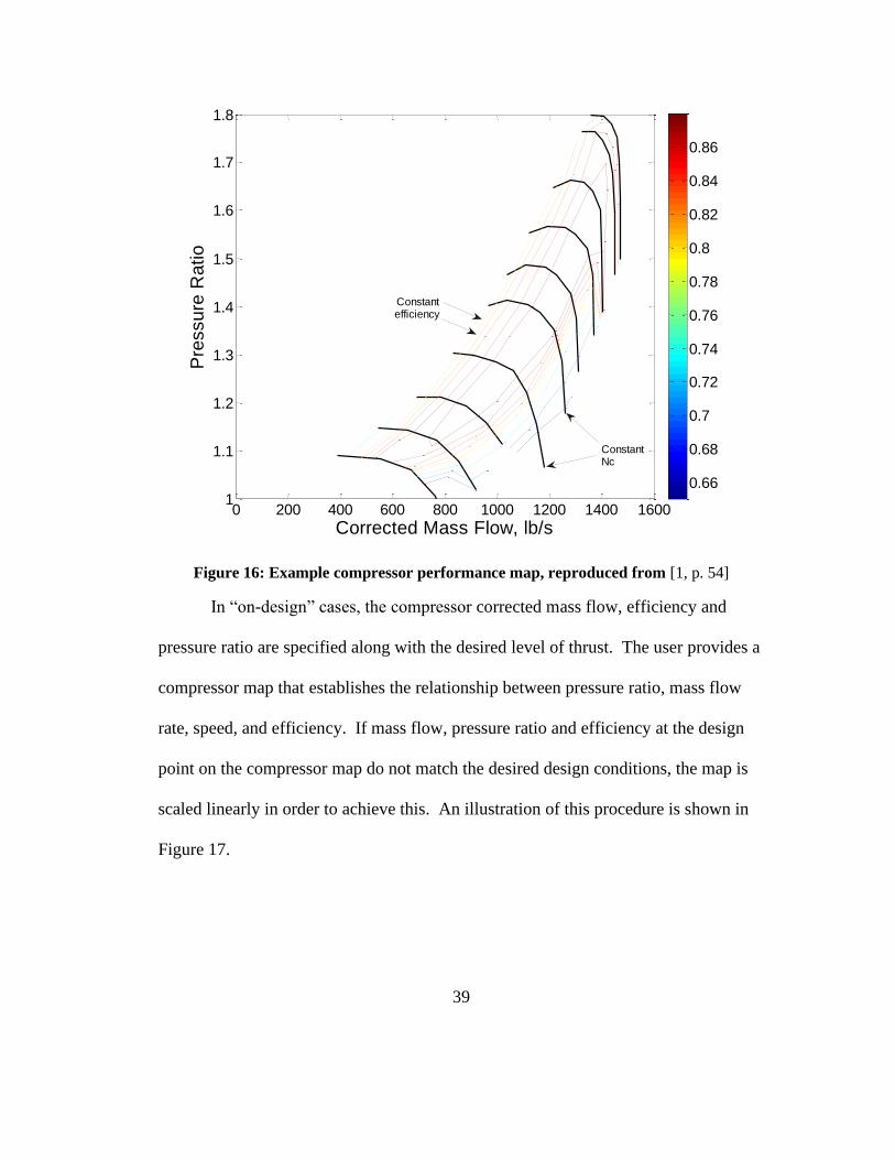
39
Figure 16: Example compressor performance map, reproduced from [1, p. 54]
In “on-design” cases, the compressor corrected mass flow, efficiency and
pressure ratio are specified along with the desired level of thrust. The user provides a
compressor map that establishes the relationship between pressure ratio, mass flow
rate, speed, and efficiency. If mass flow, pressure ratio and efficiency at the design
point on the compressor map do not match the desired design conditions, the map is
scaled linearly in order to achieve this. An illustration of this procedure is shown in
Figure 17.
0 200 400 600 800 1000 1200 1400 16001
1.1
1.2
1.3
1.4
1.5
1.6
1.7
1.8
Corrected Mass Flow, lb/s
Pre
ssure
Ratio
0.66
0.68
0.7
0.72
0.74
0.76
0.78
0.8
0.82
0.84
0.86
ConstantNc
Constantefficiency
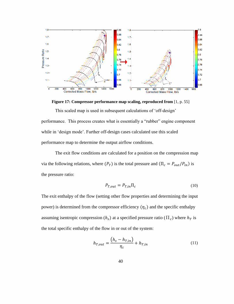
40
Figure 17: Compressor performance map scaling, reproduced from [1, p. 55]
This scaled map is used in subsequent calculations of ‘off-design’
performance. This process creates what is essentially a “rubber” engine component
while in ‘design mode’. Further off-design cases calculated use this scaled
performance map to determine the output airflow conditions.
The exit flow conditions are calculated for a position on the compression map
via the following relations, where (𝑃𝑇) is the total pressure and (Π𝑐 = 𝑃𝑜𝑢𝑡/𝑃𝑖𝑛) is
the pressure ratio:
𝑃𝑇,𝑜𝑢𝑡 = 𝑃𝑇,𝑖𝑛Π𝑐 (10)
The exit enthalpy of the flow (setting other flow properties and determining the input
power) is determined from the compressor efficiency (𝜂𝑐) and the specific enthalpy
assuming isentropic compression (ℎ𝑠) at a specified pressure ratio (Π𝑐) where ℎ𝑇 is
the total specific enthalpy of the flow in or out of the system:
ℎ𝑇,𝑜𝑢𝑡 =
(ℎ𝑠 − ℎ𝑇,𝑖𝑛)
𝜂𝑐+ ℎ𝑇,𝑖𝑛 (11)
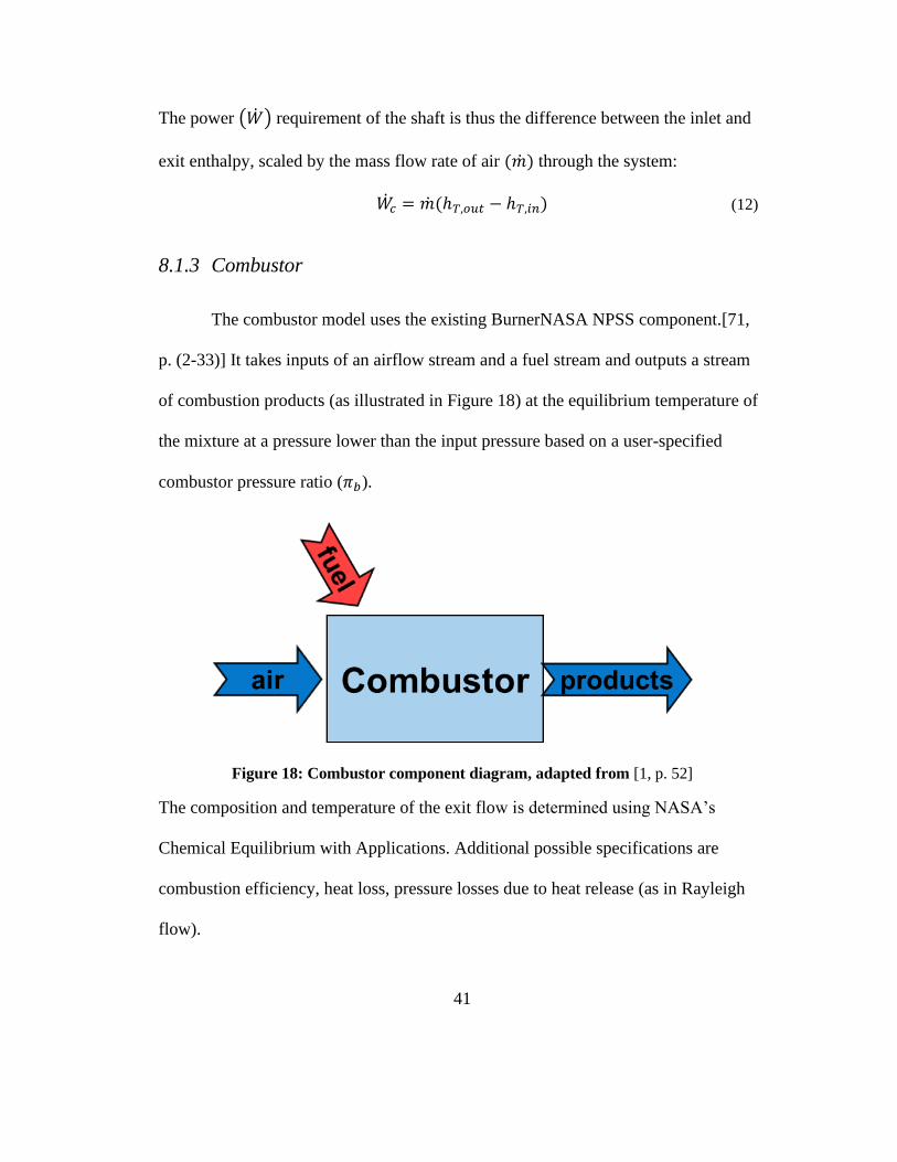
41
The power (�̇�) requirement of the shaft is thus the difference between the inlet and
exit enthalpy, scaled by the mass flow rate of air (�̇�) through the system:
�̇�𝑐 = �̇�(ℎ𝑇,𝑜𝑢𝑡 − ℎ𝑇,𝑖𝑛) (12)
8.1.3 Combustor
The combustor model uses the existing BurnerNASA NPSS component.[71,
p. (2-33)] It takes inputs of an airflow stream and a fuel stream and outputs a stream
of combustion products (as illustrated in Figure 18) at the equilibrium temperature of
the mixture at a pressure lower than the input pressure based on a user-specified
combustor pressure ratio (𝜋𝑏).
Figure 18: Combustor component diagram, adapted from [1, p. 52]
The composition and temperature of the exit flow is determined using NASA’s
Chemical Equilibrium with Applications. Additional possible specifications are
combustion efficiency, heat loss, pressure losses due to heat release (as in Rayleigh
flow).
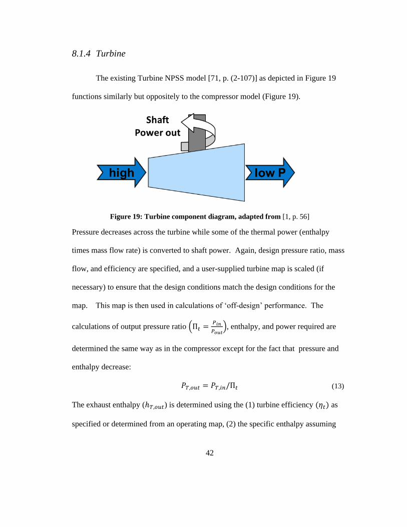
42
8.1.4 Turbine
The existing Turbine NPSS model [71, p. (2-107)] as depicted in Figure 19
functions similarly but oppositely to the compressor model (Figure 19).
Figure 19: Turbine component diagram, adapted from [1, p. 56]
Pressure decreases across the turbine while some of the thermal power (enthalpy
times mass flow rate) is converted to shaft power. Again, design pressure ratio, mass
flow, and efficiency are specified, and a user-supplied turbine map is scaled (if
necessary) to ensure that the design conditions match the design conditions for the
map. This map is then used in calculations of ‘off-design’ performance. The
calculations of output pressure ratio (Π𝑡 =𝑃𝑖𝑛
𝑃𝑜𝑢𝑡), enthalpy, and power required are
determined the same way as in the compressor except for the fact that pressure and
enthalpy decrease:
𝑃𝑇,𝑜𝑢𝑡 = 𝑃𝑇,𝑖𝑛/Π𝑡 (13)
The exhaust enthalpy (ℎ𝑇,𝑜𝑢𝑡) is determined using the (1) turbine efficiency (𝜂𝑡) as
specified or determined from an operating map, (2) the specific enthalpy assuming
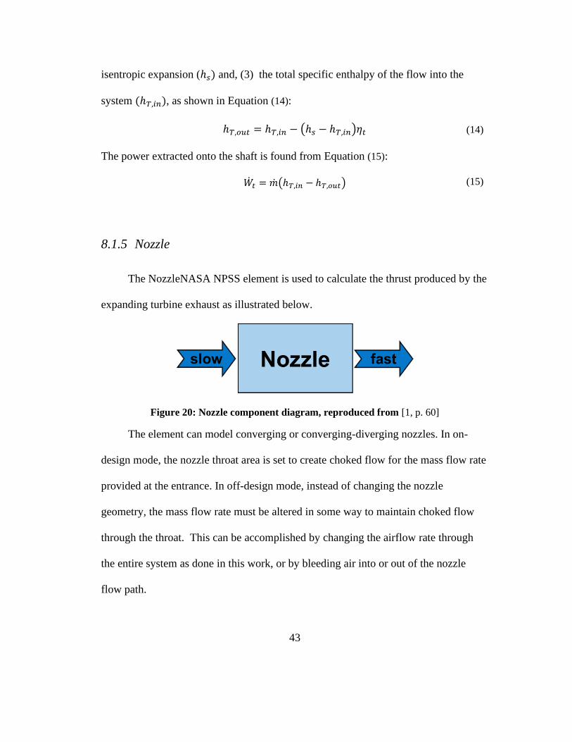
43
isentropic expansion (ℎ𝑠) and, (3) the total specific enthalpy of the flow into the
system (ℎ𝑇,𝑖𝑛), as shown in Equation (14):
ℎ𝑇,𝑜𝑢𝑡 = ℎ𝑇,𝑖𝑛 − (ℎ𝑠 − ℎ𝑇,𝑖𝑛)𝜂𝑡 (14)
The power extracted onto the shaft is found from Equation (15):
�̇�𝑡 = �̇�(ℎ𝑇,𝑖𝑛 − ℎ𝑇,𝑜𝑢𝑡) (15)
8.1.5 Nozzle
The NozzleNASA NPSS element is used to calculate the thrust produced by the
expanding turbine exhaust as illustrated below.
Figure 20: Nozzle component diagram, reproduced from [1, p. 60]
The element can model converging or converging-diverging nozzles. In on-
design mode, the nozzle throat area is set to create choked flow for the mass flow rate
provided at the entrance. In off-design mode, instead of changing the nozzle
geometry, the mass flow rate must be altered in some way to maintain choked flow
through the throat. This can be accomplished by changing the airflow rate through
the entire system as done in this work, or by bleeding air into or out of the nozzle
flow path.
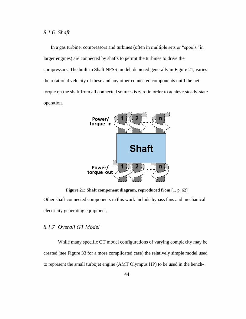
44
8.1.6 Shaft
In a gas turbine, compressors and turbines (often in multiple sets or “spools” in
larger engines) are connected by shafts to permit the turbines to drive the
compressors. The built-in Shaft NPSS model, depicted generally in Figure 21, varies
the rotational velocity of these and any other connected components until the net
torque on the shaft from all connected sources is zero in order to achieve steady-state
operation.
Figure 21: Shaft component diagram, reproduced from [1, p. 62]
Other shaft-connected components in this work include bypass fans and mechanical
electricity generating equipment.
8.1.7 Overall GT Model
While many specific GT model configurations of varying complexity may be
created (see Figure 33 for a more complicated case) the relatively simple model used
to represent the small turbojet engine (AMT Olympus HP) to be used in the bench-
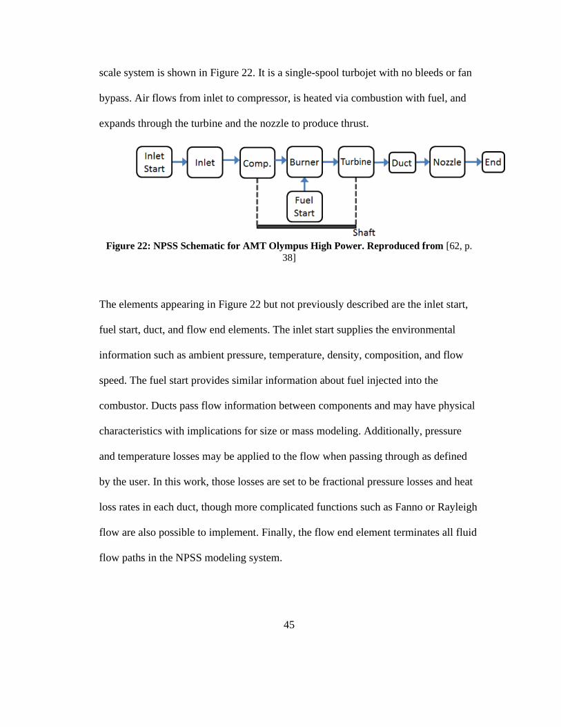
45
scale system is shown in Figure 22. It is a single-spool turbojet with no bleeds or fan
bypass. Air flows from inlet to compressor, is heated via combustion with fuel, and
expands through the turbine and the nozzle to produce thrust.
Figure 22: NPSS Schematic for AMT Olympus High Power. Reproduced from [62, p.
38]
The elements appearing in Figure 22 but not previously described are the inlet start,
fuel start, duct, and flow end elements. The inlet start supplies the environmental
information such as ambient pressure, temperature, density, composition, and flow
speed. The fuel start provides similar information about fuel injected into the
combustor. Ducts pass flow information between components and may have physical
characteristics with implications for size or mass modeling. Additionally, pressure
and temperature losses may be applied to the flow when passing through as defined
by the user. In this work, those losses are set to be fractional pressure losses and heat
loss rates in each duct, though more complicated functions such as Fanno or Rayleigh
flow are also possible to implement. Finally, the flow end element terminates all fluid
flow paths in the NPSS modeling system.
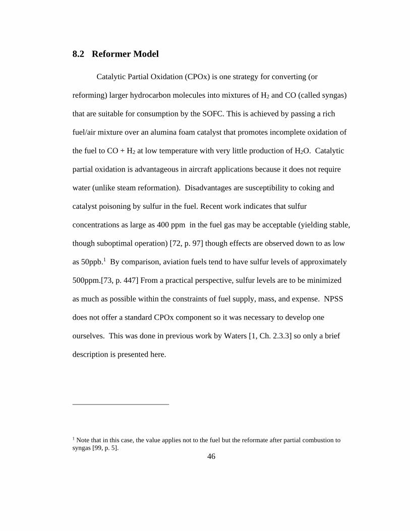
46
8.2 Reformer Model
Catalytic Partial Oxidation (CPOx) is one strategy for converting (or
reforming) larger hydrocarbon molecules into mixtures of H2 and CO (called syngas)
that are suitable for consumption by the SOFC. This is achieved by passing a rich
fuel/air mixture over an alumina foam catalyst that promotes incomplete oxidation of
the fuel to CO + H2 at low temperature with very little production of H2O. Catalytic
partial oxidation is advantageous in aircraft applications because it does not require
water (unlike steam reformation). Disadvantages are susceptibility to coking and
catalyst poisoning by sulfur in the fuel. Recent work indicates that sulfur
concentrations as large as 400 ppm in the fuel gas may be acceptable (yielding stable,
though suboptimal operation) [72, p. 97] though effects are observed down to as low
as 50ppb.1 By comparison, aviation fuels tend to have sulfur levels of approximately
500ppm.[73, p. 447] From a practical perspective, sulfur levels are to be minimized
as much as possible within the constraints of fuel supply, mass, and expense. NPSS
does not offer a standard CPOx component so it was necessary to develop one
ourselves. This was done in previous work by Waters [1, Ch. 2.3.3] so only a brief
description is presented here.
1 Note that in this case, the value applies not to the fuel but the reformate after partial combustion to
syngas [99, p. 5].
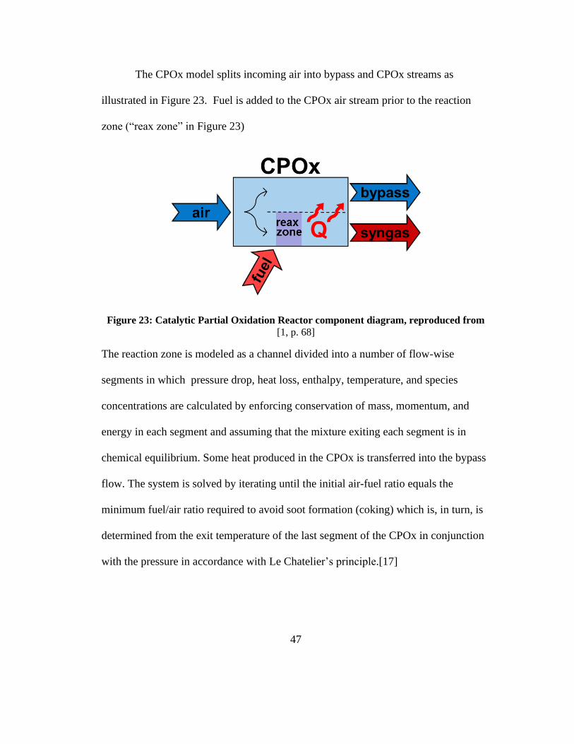
47
The CPOx model splits incoming air into bypass and CPOx streams as
illustrated in Figure 23. Fuel is added to the CPOx air stream prior to the reaction
zone (“reax zone” in Figure 23)
Figure 23: Catalytic Partial Oxidation Reactor component diagram, reproduced from
[1, p. 68]
The reaction zone is modeled as a channel divided into a number of flow-wise
segments in which pressure drop, heat loss, enthalpy, temperature, and species
concentrations are calculated by enforcing conservation of mass, momentum, and
energy in each segment and assuming that the mixture exiting each segment is in
chemical equilibrium. Some heat produced in the CPOx is transferred into the bypass
flow. The system is solved by iterating until the initial air-fuel ratio equals the
minimum fuel/air ratio required to avoid soot formation (coking) which is, in turn, is
determined from the exit temperature of the last segment of the CPOx in conjunction
with the pressure in accordance with Le Chatelier’s principle.[17]
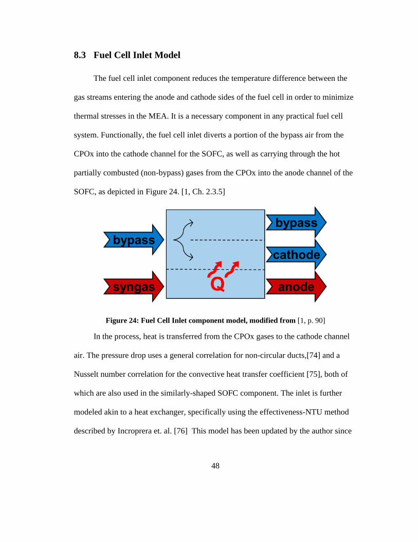
48
8.3 Fuel Cell Inlet Model
The fuel cell inlet component reduces the temperature difference between the
gas streams entering the anode and cathode sides of the fuel cell in order to minimize
thermal stresses in the MEA. It is a necessary component in any practical fuel cell
system. Functionally, the fuel cell inlet diverts a portion of the bypass air from the
CPOx into the cathode channel for the SOFC, as well as carrying through the hot
partially combusted (non-bypass) gases from the CPOx into the anode channel of the
SOFC, as depicted in Figure 24. [1, Ch. 2.3.5]
Figure 24: Fuel Cell Inlet component model, modified from [1, p. 90]
In the process, heat is transferred from the CPOx gases to the cathode channel
air. The pressure drop uses a general correlation for non-circular ducts,[74] and a
Nusselt number correlation for the convective heat transfer coefficient [75], both of
which are also used in the similarly-shaped SOFC component. The inlet is further
modeled akin to a heat exchanger, specifically using the effectiveness-NTU method
described by Incroprera et. al. [76] This model has been updated by the author since

49
the prior work to properly calculate heat losses for each segment progressing linearly
along the length of the inlet.
8.4 Solid Oxide Fuel Cell Model
8.4.1 Overall Configuration
The fuel cell model used in this work is identical to that developed by Waters [1, Ch.
2.3.4], except for variations in the specific geometry of particular GT-SOFC designs
which depend on the scenario of interest and the choice of which variables are
designated as dependent and independent for the solver. Specific properties that
change include the SOFC length, fuel flow rate, insulation thickness, and number of
membrane electrode assembly units per SOFC “stack”. The physical structure of the
fuel cell consists of annular rings (Figure 25) arranged around a cylindrical engine
section. Calculations are simplified by assuming that the diameters of the rings are
much larger than the width of the flow passages and thus can be approximated as flat.
Each stack is assumed to be a certain number (𝑁𝑟𝑒𝑝) of repeating units thick. Each
repeating unit (illustrated with dotted lines in the figure) consists of an anode channel
with half cathode channels above and below that are separated from the anode
channel by MEAs. the symmetry of the annular configuration simplifies heat transfer
calculations because heat only flows through the top and bottom of the stack and the
boundary conditions on the left and right edges of the stack can be assumed to be the
same. As a result, the calculations need only be performed for a single stack.
50
Figure 25. Assumed layout of CPOx/SOFC Components.
The fuel cell model is like the reformer’s in that it is broken into a series of
segments in the flow direction (see section 3.4.3.2 below). Pressure drop, heat loss,
diffusion of 𝑂2− ions through the MEA, and equilibrium (this time also considering
reactions on the anode and cathode surfaces) are computed in each segment.
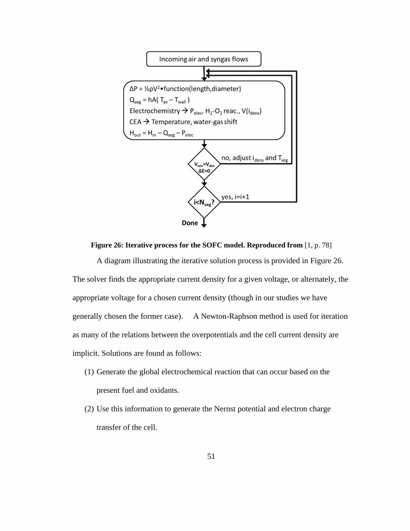
51
Figure 26: Iterative process for the SOFC model. Reproduced from [1, p. 78]
A diagram illustrating the iterative solution process is provided in Figure 26.
The solver finds the appropriate current density for a given voltage, or alternately, the
appropriate voltage for a chosen current density (though in our studies we have
generally chosen the former case). A Newton-Raphson method is used for iteration
as many of the relations between the overpotentials and the cell current density are
implicit. Solutions are found as follows:
(1) Generate the global electrochemical reaction that can occur based on the
present fuel and oxidants.
(2) Use this information to generate the Nernst potential and electron charge
transfer of the cell.

52
(3) Assume a current-density target and use it to establish the rate of flow of
various chemical species into and out of the anode and cathode to match the
required number of electrons produced.
(4) Use the dusty gas model to determine the rate of 𝑂2− conduction through the
MEA.
(5) Use the species concentrations in the anode and cathode flows to generate
concentration overpotentials at both electrodes.
(6) Use the Butler-Volmer equation to infer the activation overpotentials for both
anode and cathode.
(7) Evaluate the ohmic and interface overpotentials.
(8) Calculate the leakage overpotential from a known initial leakage rate at the
open circuit condition. The unknown 𝑖𝑚𝑎𝑥 value is found by iteration.
(9) Determine the final cell voltage by summing the overpotentials. If a specific
voltage is sought, the assumed current density is lowered or raised, depending
on whether the voltage found initially was too low or too high.
The iterative process is repeated for flow down a channel (into the page of
Figure 25) where the channel is divided into a number of segments as shown in
Figure 27.
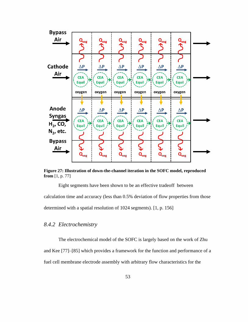
53
Figure 27: Illustration of down-the-channel iteration in the SOFC model, reproduced
from [1, p. 77]
Eight segments have been shown to be an effective tradeoff between
calculation time and accuracy (less than 0.5% deviation of flow properties from those
determined with a spatial resolution of 1024 segments). [1, p. 156]
8.4.2 Electrochemistry
The electrochemical model of the SOFC is largely based on the work of Zhu
and Kee [77]–[85] which provides a framework for the function and performance of a
fuel cell membrane electrode assembly with arbitrary flow characteristics for the
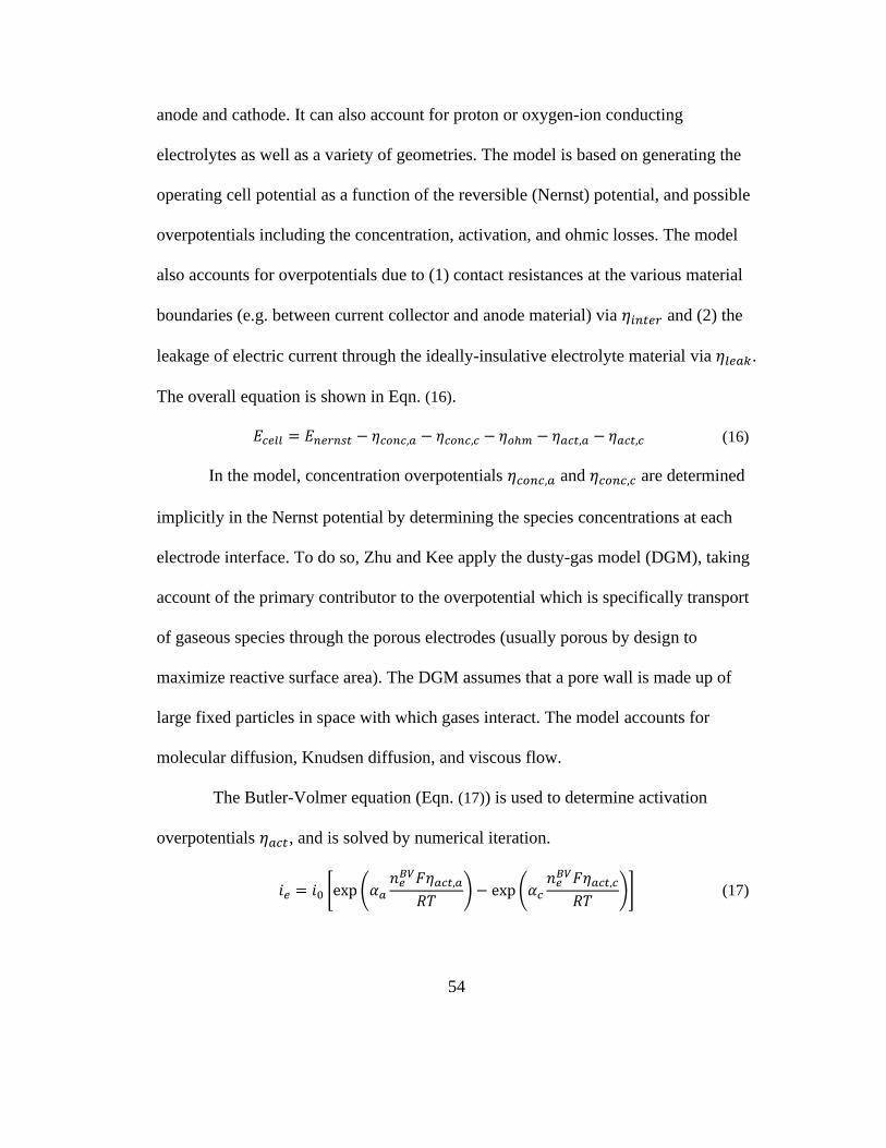
54
anode and cathode. It can also account for proton or oxygen-ion conducting
electrolytes as well as a variety of geometries. The model is based on generating the
operating cell potential as a function of the reversible (Nernst) potential, and possible
overpotentials including the concentration, activation, and ohmic losses. The model
also accounts for overpotentials due to (1) contact resistances at the various material
boundaries (e.g. between current collector and anode material) via 𝜂𝑖𝑛𝑡𝑒𝑟 and (2) the
leakage of electric current through the ideally-insulative electrolyte material via 𝜂𝑙𝑒𝑎𝑘.
The overall equation is shown in Eqn. (16).
𝐸𝑐𝑒𝑙𝑙 = 𝐸𝑛𝑒𝑟𝑛𝑠𝑡 − 𝜂𝑐𝑜𝑛𝑐,𝑎 − 𝜂𝑐𝑜𝑛𝑐,𝑐 − 𝜂𝑜ℎ𝑚 − 𝜂𝑎𝑐𝑡,𝑎 − 𝜂𝑎𝑐𝑡,𝑐 (16)
In the model, concentration overpotentials 𝜂𝑐𝑜𝑛𝑐,𝑎 and 𝜂𝑐𝑜𝑛𝑐,𝑐 are determined
implicitly in the Nernst potential by determining the species concentrations at each
electrode interface. To do so, Zhu and Kee apply the dusty-gas model (DGM), taking
account of the primary contributor to the overpotential which is specifically transport
of gaseous species through the porous electrodes (usually porous by design to
maximize reactive surface area). The DGM assumes that a pore wall is made up of
large fixed particles in space with which gases interact. The model accounts for
molecular diffusion, Knudsen diffusion, and viscous flow.
The Butler-Volmer equation (Eqn. (17)) is used to determine activation
overpotentials 𝜂𝑎𝑐𝑡, and is solved by numerical iteration.
𝑖𝑒 = 𝑖0 [exp (𝛼𝑎
𝑛𝑒𝐵𝑉𝐹𝜂𝑎𝑐𝑡,𝑎𝑅𝑇
) − exp(𝛼𝑐𝑛𝑒𝐵𝑉𝐹𝜂𝑎𝑐𝑡,𝑐𝑅𝑇
)] (17)

55
Ohmic resistance - essentially the losses due to the inherent ‘wire’ resistance
experienced by charge flowing through the electrodes and electrolyte - is linear with
respect to current and the total resistance from all sources. The total resistance is
calculated from the electrode inherent resistance, added to the ion conductivity
through the electrolyte. Ion conductivity is the primary source of resistance and is a
function of temperature and the activation energy of ionic transport through the
specific electrolyte.
More detailed information about the implementation of the SOFC
electrochemistry model is available elsewhere. [1, Ch. 2.3.4], [17]
8.4.3 Heat Transfer and Pressure Loss
Broadly, heat transfer (and thus stack temperature) is controlled by the
thickness of the layer of insulation (𝑡𝑖𝑛𝑠) on the top and bottom edges of the stack.
The bypass air stream from the fuel cell inlet passes around the outside of the annular
rings (with the insulation in between) allowing for cooling of the SOFC. Internal to
the SOFC, both the heat transfer and pressure loss coefficient calculations are based
on work by Muzychka and Yovanovich for non-circular ducts. [74], [75]
The heat transfer method is a proposed general model that combines the results
of fully developed flow, Graetz flow, and laminar boundary flow regimes, yielding an
expression for the average Nusselt number for uniform temperature walls and set for
rectangular ducts.[75] The actual heat loss calculations are performed by solving a
56
discrete finite volume problem over repeating sections of the fuel cell channels as
shown in Figure 28.
Figure 28: Discretization scheme for heat transfer calculations. Reproduced from [17]
Heat transfer from the channel flow to the wall surfaces applies the Nusselt number as
determined previously via forced convection. Further heat transfer details may be
found in both section 2.3.4 and Appendix D of Waters.[1]
8.5 Fuel Cell Assembly Model
The NPSS model of the CPOx/SOFC assembly shown in Figure 29 includes all
of the fuel cell related components: (1) a splitter to divert some of the flow exiting the
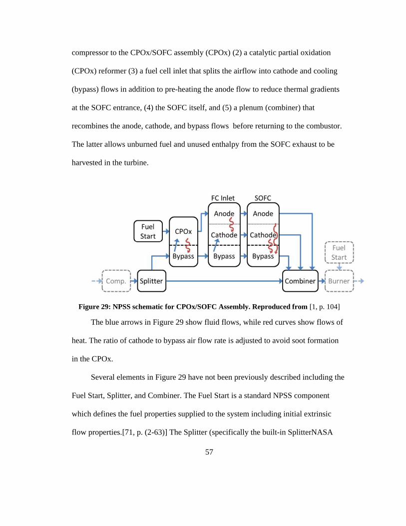
57
compressor to the CPOx/SOFC assembly (CPOx) (2) a catalytic partial oxidation
(CPOx) reformer (3) a fuel cell inlet that splits the airflow into cathode and cooling
(bypass) flows in addition to pre-heating the anode flow to reduce thermal gradients
at the SOFC entrance, (4) the SOFC itself, and (5) a plenum (combiner) that
recombines the anode, cathode, and bypass flows before returning to the combustor.
The latter allows unburned fuel and unused enthalpy from the SOFC exhaust to be
harvested in the turbine.
Figure 29: NPSS schematic for CPOx/SOFC Assembly. Reproduced from [1, p. 104]
The blue arrows in Figure 29 show fluid flows, while red curves show flows of
heat. The ratio of cathode to bypass air flow rate is adjusted to avoid soot formation
in the CPOx.
Several elements in Figure 29 have not been previously described including the
Fuel Start, Splitter, and Combiner. The Fuel Start is a standard NPSS component
which defines the fuel properties supplied to the system including initial extrinsic
flow properties.[71, p. (2-63)] The Splitter (specifically the built-in SplitterNASA
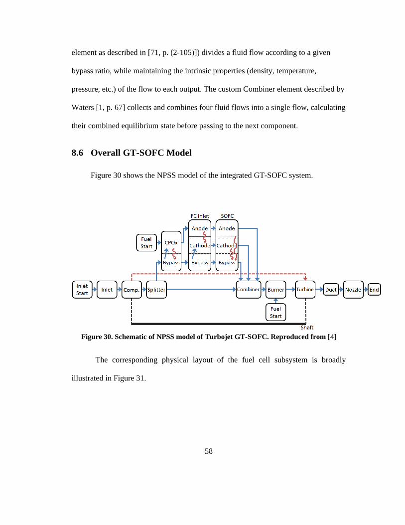
58
element as described in [71, p. (2-105)]) divides a fluid flow according to a given
bypass ratio, while maintaining the intrinsic properties (density, temperature,
pressure, etc.) of the flow to each output. The custom Combiner element described by
Waters [1, p. 67] collects and combines four fluid flows into a single flow, calculating
their combined equilibrium state before passing to the next component.
8.6 Overall GT-SOFC Model
Figure 30 shows the NPSS model of the integrated GT-SOFC system.
Figure 30. Schematic of NPSS model of Turbojet GT-SOFC. Reproduced from [4]
The corresponding physical layout of the fuel cell subsystem is broadly
illustrated in Figure 31.
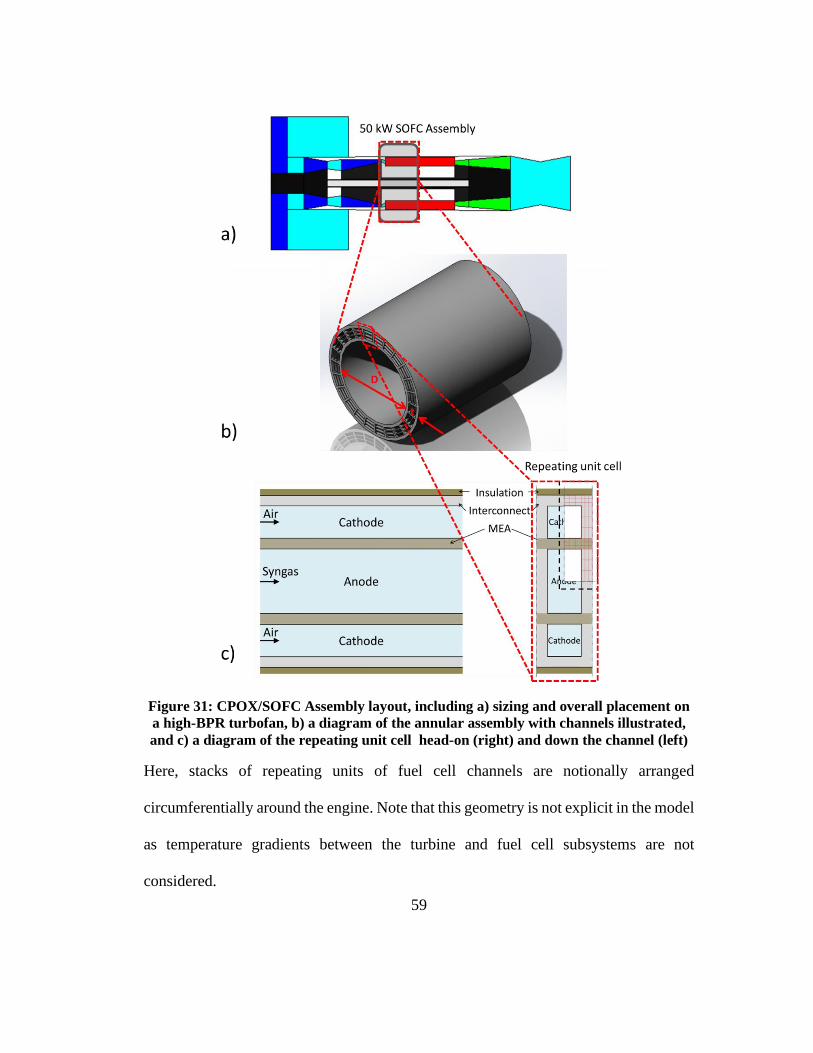
59
Figure 31: CPOX/SOFC Assembly layout, including a) sizing and overall placement on
a high-BPR turbofan, b) a diagram of the annular assembly with channels illustrated,
and c) a diagram of the repeating unit cell head-on (right) and down the channel (left)
Here, stacks of repeating units of fuel cell channels are notionally arranged
circumferentially around the engine. Note that this geometry is not explicit in the model
as temperature gradients between the turbine and fuel cell subsystems are not
considered.
60
Furthermore, while the general size is consistent with the notional arrangement,
the analysis is performed under the assumption that all of the stacks are flat, essentially
“unwrapped” from the engine—which can be less reasonable an assumption for a small
laboratory-scale gas turbine such as the AMT Olympus [61], [62] than it is for a larger-
diameter HALE UAV or passenger jet.
8.7 Mass Estimation
While the thermodynamic benefits of an integrated GT-SOFC are clear in
ground applications, mass and volume are additional key factors for evaluating the
usefulness and performance in aircraft. Should an efficient integrated GT-SOFC be
too large or heavy, specific power and power density for the aircraft overall will fall,
lowering performance by increasing profile drag or increasing the required angle of
attack to counteract the larger system mass. As such, accurate modeling of the mass
and volume of the gas turbine, SOFC assembly, and supporting hardware is an
essential extra step in determining the viability of a GT-SOFC system for aircraft. [1,
Ch. 4] This section will expand on the models used for each component. Note that
these models are not relevant to the design of the lab-scale model presented in
Chapter 10.1, since it is not intended to fly.
8.7.1 Gas Turbine
The gas turbine mass is determined using a model based on Onat and Klees
[86] and Sanghi et. al., [87] which generates a system mass by determining the sizing

61
requirements piece by piece based on the operating conditions of the engine model
state. The full model implemented (here applied to mass and aerodynamic drag
analysis) is identical to that used by Waters, which has been validated to be accurate
to within 14% for a range of known GT engines and 10% for American GT engines.
[1, Ch. 4.2] Note that mass and volume estimation is not relevant for the analysis lab-
scale model based on the AMT Olympus turbojet, though in such a case, the mass
model of the GT would be simply the mass of the Olympus as provided.
8.7.2 Fuel Cell
The CPOx/SOFC assembly mass is determined in a similarly piecewise fashion to
that of the gas turbine. However, often set values for the dimensions of the system
and channel are chosen ahead of the calculation, rather than being determined by the
system operating state, as described in section 7.2. Again, the full mass/volume model
is identical to the one employed by Waters. [1, Ch. 4.3] A notable design
consideration is a mass-advantage to increasing radial stack size over adding entirely
new stacks due to the mass of the interconnect wall and insulation.
8.7.3 Additional Hardware
In addition to the GT and CPOX/SOFC assembly, there is a duct that contains
the assembly and mounting bolts that support the weight of the assembly added to the
engine. The size of the duct is set to be large enough to accommodate the length and
area of the SOFC, including the cooling bypass flow. The area (𝐴𝑑𝑢𝑐𝑡) is represented
62
by Equation (18). 𝐴𝑏𝑝 is the area of the bypass duct, in turn determined by the cooling
air mass flow rate �̇�𝑏𝑝, the density (𝜌𝑏𝑝) of air diverted from the compressor, and the
design bypass flow velocity (𝑣𝑏𝑝), which is set in this work to be 100 m/s. 𝐴𝑆𝑂𝐹𝐶 is
the area of the fuel cell anode and cathode ducts, determined by a the number of fuel
cell anode/cathode channel units (𝑁𝐹𝐶) multiplied by the area of a single SOFC stack
unit including walls. The resulting inner diameter (𝐷𝑖) and outer diameter (𝐷𝑜) of the
duct are set by the diameter of the engine (set by the engine operating requirements)
and the area of the duct (as shown in Equation (19)) respectively.
𝐴𝑑𝑢𝑐𝑡 = 𝐴𝑏𝑝 + 𝐴𝑆𝑂𝐹𝐶 =
�̇�𝑏𝑝
𝜌𝑏𝑝𝑣𝑏𝑝+ 𝑁𝐹𝐶𝐴𝐹𝐶,𝑢𝑛𝑖𝑡 (18)
𝐷𝑜 = √𝐷𝑖2 +
4
𝜋𝐴𝑑𝑢𝑐𝑡 (19)
In one variant of the external aerodynamic model (see chapter 9.1 and Figure 35
in particular), the duct winds back once, doubling its radial area. In that case the
second equation becomes:
𝐷𝑜 = √𝐷𝑖2 +
8
𝜋𝐴𝑑𝑢𝑐𝑡 (20)
The mass of this duct depends on a wall thickness and material density that are
specified in the model. Again, the model is identical to the one employed by Waters.
[1, Ch. 4.3.4]

63
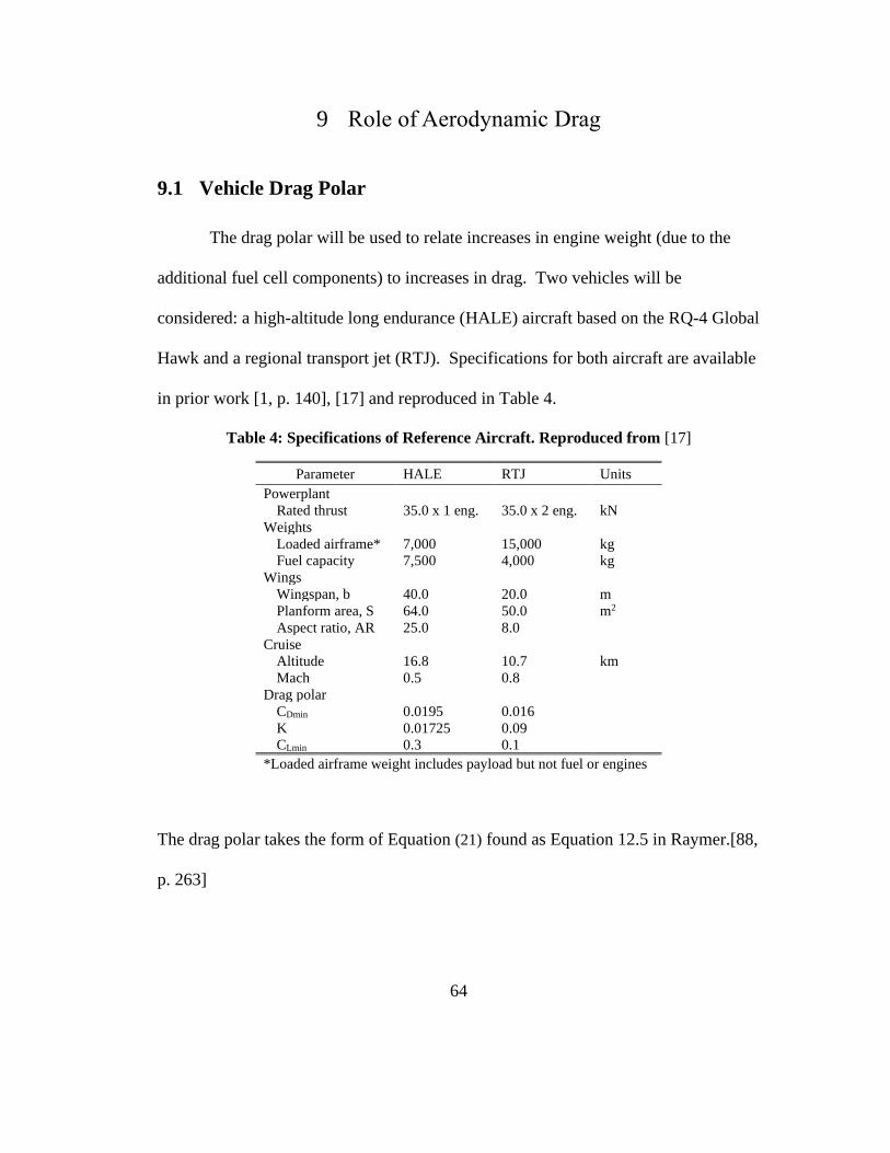
64
9 Role of Aerodynamic Drag
9.1 Vehicle Drag Polar
The drag polar will be used to relate increases in engine weight (due to the
additional fuel cell components) to increases in drag. Two vehicles will be
considered: a high-altitude long endurance (HALE) aircraft based on the RQ-4 Global
Hawk and a regional transport jet (RTJ). Specifications for both aircraft are available
in prior work [1, p. 140], [17] and reproduced in Table 4.
Table 4: Specifications of Reference Aircraft. Reproduced from [17]
Parameter HALE RTJ Units
Powerplant
Rated thrust 35.0 x 1 eng. 35.0 x 2 eng. kN
Weights
Loaded airframe* 7,000 15,000 kg
Fuel capacity 7,500 4,000 kg
Wings
Wingspan, b 40.0 20.0 m
Planform area, S 64.0 50.0 m2
Aspect ratio, AR 25.0 8.0
Cruise
Altitude 16.8 10.7 km
Mach 0.5 0.8
Drag polar
CDmin 0.0195 0.016
K 0.01725 0.09
CLmin 0.3 0.1
*Loaded airframe weight includes payload but not fuel or engines
The drag polar takes the form of Equation (21) found as Equation 12.5 in Raymer.[88,
p. 263]
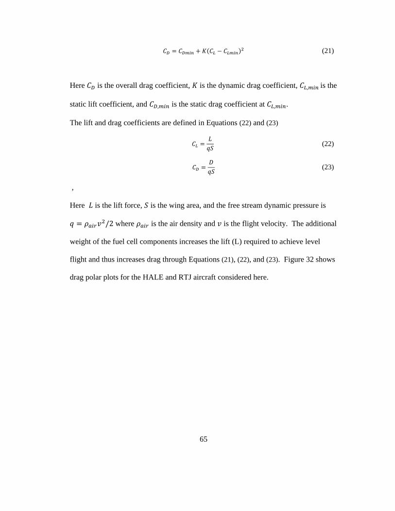
65
𝐶𝐷 = 𝐶𝐷𝑚𝑖𝑛 + 𝐾(𝐶𝐿 − 𝐶𝐿𝑚𝑖𝑛)2 (21)
Here 𝐶𝐷 is the overall drag coefficient, 𝐾 is the dynamic drag coefficient, 𝐶𝐿,𝑚𝑖𝑛 is the
static lift coefficient, and 𝐶𝐷,𝑚𝑖𝑛 is the static drag coefficient at 𝐶𝐿,𝑚𝑖𝑛.
The lift and drag coefficients are defined in Equations (22) and (23)
𝐶𝐿 =
𝐿
𝑞𝑆 (22)
𝐶𝐷 =
𝐷
𝑞𝑆 (23)
,
Here 𝐿 is the lift force, 𝑆 is the wing area, and the free stream dynamic pressure is
𝑞 = 𝜌𝑎𝑖𝑟𝑣2/2 where 𝜌𝑎𝑖𝑟 is the air density and 𝑣 is the flight velocity. The additional
weight of the fuel cell components increases the lift (L) required to achieve level
flight and thus increases drag through Equations (21), (22), and (23). Figure 32 shows
drag polar plots for the HALE and RTJ aircraft considered here.
66
Figure 32: Drag Polar plots of High-Altitude Long-Endurance (HALE) and Regional
Transport Jet (RTJ) aircraft
9.2 NPSS models for HALE and RTJ aircraft
The HALE and RTJ aircraft are equipped with turbofan engines so the NPSS
model discussed in section 8.6 is extended to account for the additional
turbomachinery as illustrated below in Figure 33.
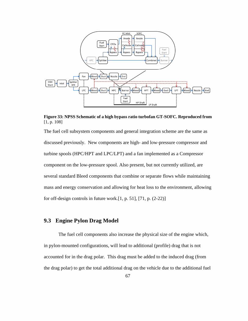
67
Figure 33: NPSS Schematic of a high bypass ratio turbofan GT-SOFC. Reproduced from
[1, p. 108]
The fuel cell subsystem components and general integration scheme are the same as
discussed previously. New components are high- and low-pressure compressor and
turbine spools (HPC/HPT and LPC/LPT) and a fan implemented as a Compressor
component on the low-pressure spool. Also present, but not currently utilized, are
several standard Bleed components that combine or separate flows while maintaining
mass and energy conservation and allowing for heat loss to the environment, allowing
for off-design controls in future work.[1, p. 51], [71, p. (2-22)]
9.3 Engine Pylon Drag Model
The fuel cell components also increase the physical size of the engine which,
in pylon-mounted configurations, will lead to additional (profile) drag that is not
accounted for in the drag polar. This drag must be added to the induced drag (from
the drag polar) to get the total additional drag on the vehicle due to the additional fuel

68
cell components. Waters placed the additional mass/volume of the SOFC system
placed in an annular ring around the outside of the engine as illustrated in Figure 34
[1, Ch. 7.3]. In doing so, he applied the following drag model added drag components
on top of the standard drag polar of the given aircraft profile (here a HALE aircraft
similar to the Global Hawk, and a regional transport jet (RTJ)).
The drag model assumes an annular configuration of the CPOx/SOFC
assembly wrapping around the combustor section of the gas turbine as shown in
Figure 34. Note that for this turbofan configuration, the core of the gas turbine is
largely cylindrical. The assembly sits around the outside of the engine core protruding
a distance (𝛿)) into the secondary bypass fan flow. The assembly exhausts into the
combustor 20 cm downstream axially. Fairings upstream and downstream of the
protrusion smooth the flow of air past the assembly. The minimum length of the
assembly is constrained by the fixed compressor discharge plane and combustor
injection point.
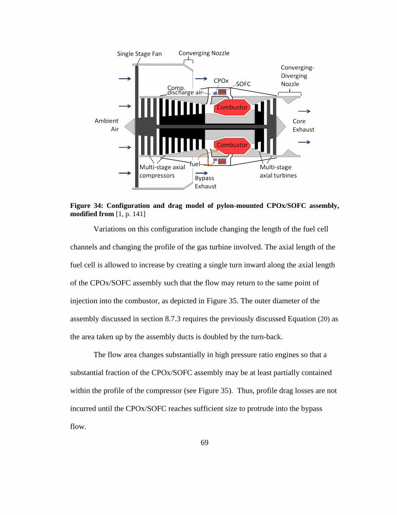
69
Figure 34: Configuration and drag model of pylon-mounted CPOx/SOFC assembly,
modified from [1, p. 141]
Variations on this configuration include changing the length of the fuel cell
channels and changing the profile of the gas turbine involved. The axial length of the
fuel cell is allowed to increase by creating a single turn inward along the axial length
of the CPOx/SOFC assembly such that the flow may return to the same point of
injection into the combustor, as depicted in Figure 35. The outer diameter of the
assembly discussed in section 8.7.3 requires the previously discussed Equation (20) as
the area taken up by the assembly ducts is doubled by the turn-back.
The flow area changes substantially in high pressure ratio engines so that a
substantial fraction of the CPOx/SOFC assembly may be at least partially contained
within the profile of the compressor (see Figure 35). Thus, profile drag losses are not
incurred until the CPOx/SOFC reaches sufficient size to protrude into the bypass
flow.
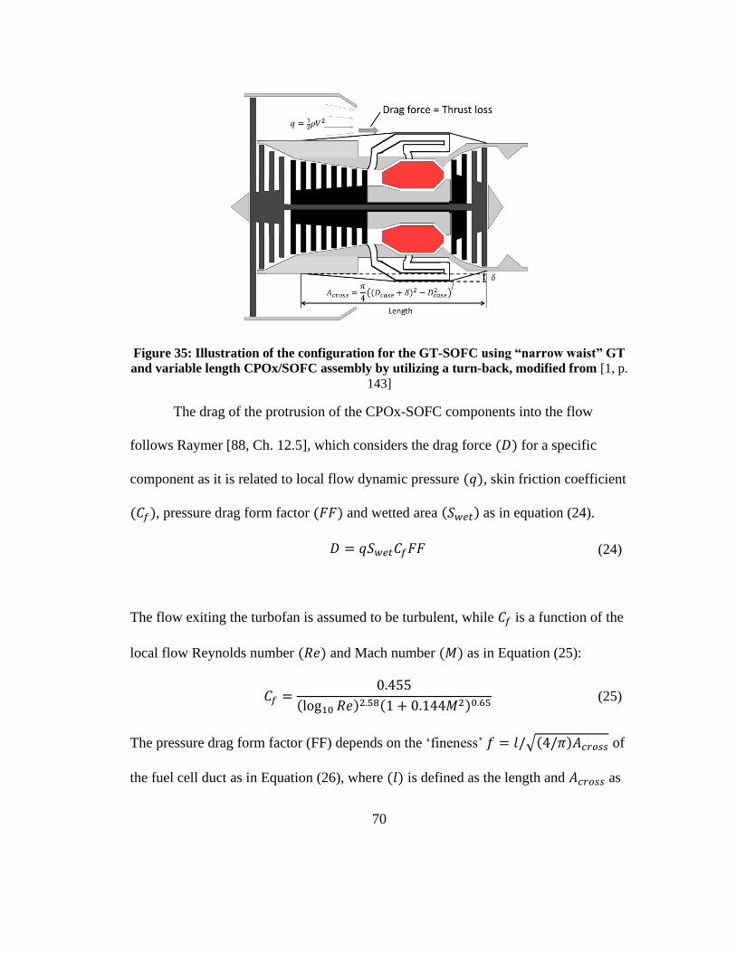
70
Figure 35: Illustration of the configuration for the GT-SOFC using “narrow waist” GT
and variable length CPOx/SOFC assembly by utilizing a turn-back, modified from [1, p.
143]
The drag of the protrusion of the CPOx-SOFC components into the flow
follows Raymer [88, Ch. 12.5], which considers the drag force (𝐷) for a specific
component as it is related to local flow dynamic pressure (𝑞), skin friction coefficient
(𝐶𝑓), pressure drag form factor (𝐹𝐹) and wetted area (𝑆𝑤𝑒𝑡) as in equation (24).
𝐷 = 𝑞𝑆𝑤𝑒𝑡𝐶𝑓𝐹𝐹 (24)
The flow exiting the turbofan is assumed to be turbulent, while 𝐶𝑓 is a function of the
local flow Reynolds number (𝑅𝑒) and Mach number (𝑀) as in Equation (25):
𝐶𝑓 =
0.455
(log10 𝑅𝑒)2.58(1 + 0.144𝑀2)0.65 (25)
The pressure drag form factor (FF) depends on the ‘fineness’ 𝑓 = 𝑙/√(4/𝜋)𝐴𝑐𝑟𝑜𝑠𝑠 of
the fuel cell duct as in Equation (26), where (𝑙) is defined as the length and 𝐴𝑐𝑟𝑜𝑠𝑠 as
71
the profile cross section of the GT-SOFC core (not counting secondary flow channels,
i.e. fan flow).
𝐹𝐹 = 1 + 60 𝑓3⁄ + 𝑓 400⁄ (26)
The profile drag force is added to the induced drag force from the vehicle drag polar
to estimate the overall thrust required to maintain level flight.
9.4 Fuel Cell Configurations
Since the electric power generated is assumed to be applied to secondary
purposes rather than propulsion, any increase in electrical demand will increase drag
and thus the fuel flow rate.
Recalling the model of the SOFC described in section 8.4.1, there are several
ways to increase electrical generation capacity. First, we can simply change the
number of SOFC rings around the GT which is equivalent to changing the number of
“stacks” in any other fuel cell scenario. From a real-world perspective, this is the
most common method as generally a single stack size is designed and manufactured.
An alternative is to vary the size of the stack itself. This is less
convenient/economical to manufacture but is more mass/volume efficient while also
changing the stack’s heat transfer properties. Both approaches increase the radial size
of the CPOx/SOFC assembly leading to more drag.
Another possibility is to grow the cell axially instead of radially as shown in
Figure 35. This allows the length to vary up to the physical limits of the GT core
whether that is the end of the nozzle, or of the “narrow waist” of some engines.
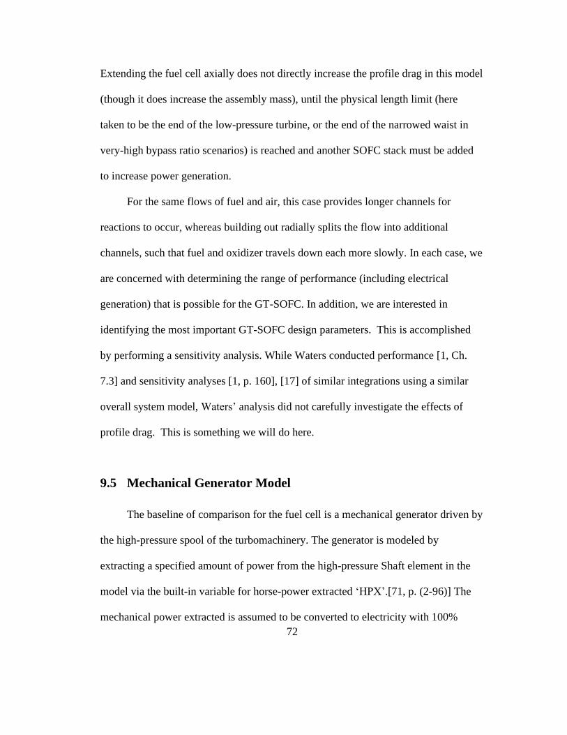
72
Extending the fuel cell axially does not directly increase the profile drag in this model
(though it does increase the assembly mass), until the physical length limit (here
taken to be the end of the low-pressure turbine, or the end of the narrowed waist in
very-high bypass ratio scenarios) is reached and another SOFC stack must be added
to increase power generation.
For the same flows of fuel and air, this case provides longer channels for
reactions to occur, whereas building out radially splits the flow into additional
channels, such that fuel and oxidizer travels down each more slowly. In each case, we
are concerned with determining the range of performance (including electrical
generation) that is possible for the GT-SOFC. In addition, we are interested in
identifying the most important GT-SOFC design parameters. This is accomplished
by performing a sensitivity analysis. While Waters conducted performance [1, Ch.
7.3] and sensitivity analyses [1, p. 160], [17] of similar integrations using a similar
overall system model, Waters’ analysis did not carefully investigate the effects of
profile drag. This is something we will do here.
9.5 Mechanical Generator Model
The baseline of comparison for the fuel cell is a mechanical generator driven by
the high-pressure spool of the turbomachinery. The generator is modeled by
extracting a specified amount of power from the high-pressure Shaft element in the
model via the built-in variable for horse-power extracted ‘HPX’.[71, p. (2-96)] The
mechanical power extracted is assumed to be converted to electricity with 100%

73
efficiency. The generator is assumed to cause no additional profile-drag by being held
fully within the body of the turbofan hub (see Figure 3), but the generator does apply
a mass penalty that becomes a part of the total aircraft mass in the drag polar. The
mass of the mechanical generator is determined from a given specific power of the
generator, here bracketed between two cases of 1kW/kg and 5kW/kg, as have been
used in prior work[1, Ch. 7.3.2], [17] and in a similar range to the survey of electric
motors shown by Ng and Datta in Figure 24 of [14].
Applying this to the HALE GT model operating in cruise conditions (M=0.5 @
55kft) and solving for progressively-higher levels of power extraction from the shaft
yields the plot of fuel consumption vs. electric power fraction presented in Figure 36.
The limitation on power extraction in both cases is determined by the turbine inlet
temperature (TIT) limit which, in turn, is set by the materials and design of the
turbine. Here it is assumed to be 1600K.
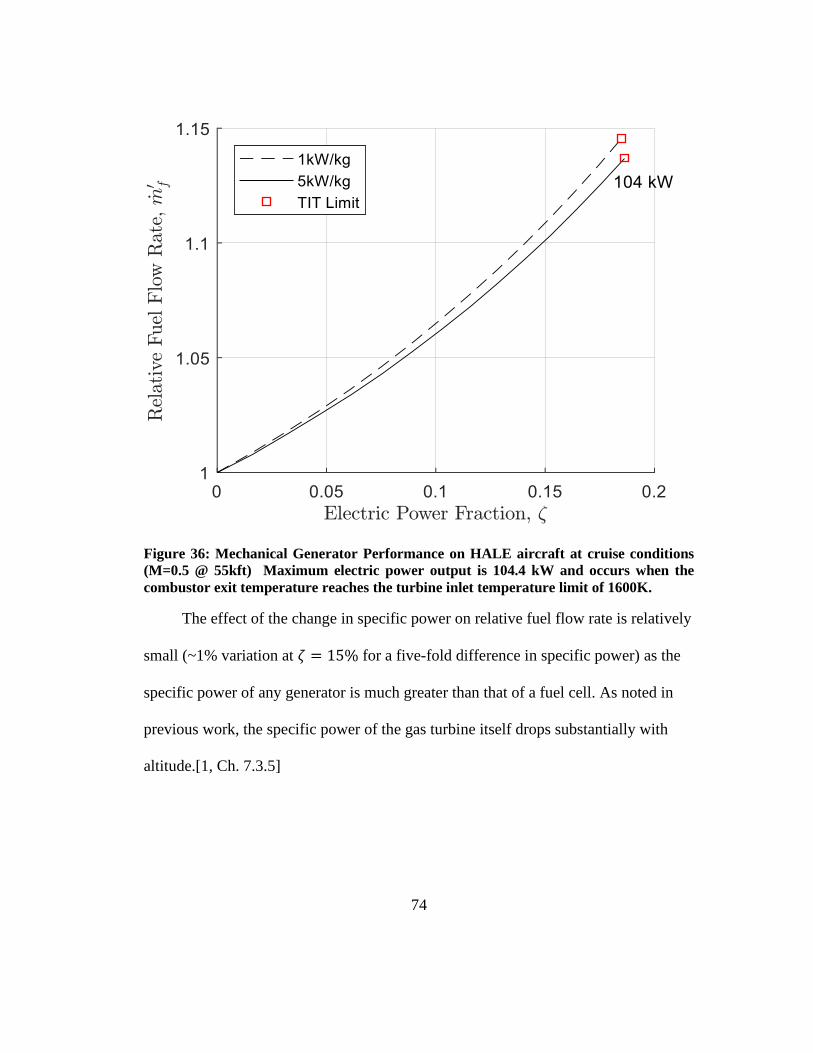
74
Figure 36: Mechanical Generator Performance on HALE aircraft at cruise conditions
(M=0.5 @ 55kft) Maximum electric power output is 104.4 kW and occurs when the
combustor exit temperature reaches the turbine inlet temperature limit of 1600K.
The effect of the change in specific power on relative fuel flow rate is relatively
small (~1% variation at 𝜁 = 15% for a five-fold difference in specific power) as the
specific power of any generator is much greater than that of a fuel cell. As noted in
previous work, the specific power of the gas turbine itself drops substantially with
altitude.[1, Ch. 7.3.5]

75
9.6 GT-SOFC Results
Both duct configurations have been considered when modeling the high bypass
ratio turbofan in the HALE aircraft. To-scale layouts of the configurations are
provided in Figure 37. The figure illustrates three cases, each building off a turbofan
with a bypass ratio of 5 and an overall pressure ratio (OPR) of 24, operated at cruise
conditions (M=0.5 @ 55kft). The yellow and bold-outlined annular section around
the combustor section (red) in each diagram represents the reformer and fuel cell
subsystems, designed to operate at a specific power level (50 kW and 250 kW are
considered here) using a fixed value of 𝑁𝑟𝑒𝑝 = 18 in the fuel cell, with 186 units per
stack (for a total width of 3.6 ft). Either the number of annular stacks (1-5) or the fuel
cell length (0.2-1.48 meters) is varied to meet the required electrical load. The ranges
allowed for each configuration are based on reasonable physical limits; in particular
the axial length is required to fit between the compressor exhaust plane and the
turbine exhaust plane using a single turn-back, while the radial growth is limited to
the fan diameter of the turbofan engine which completely blocks the flow.
Other engines, including turbojets, low bypass ratio turbofans, and “narrow-
waisted” (i.e. very high bypass ratio and/or pressure ratio) turbofans have all been
evaluated previously at a number of conditions including takeoff and idling (sea-
level-static conditions) as well as at varying altitudes and Mach numbers.[1, Ch.
7][17]
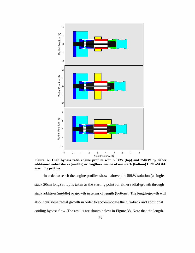
76
Figure 37: High bypass ratio engine profiles with 50 kW (top) and 250kW by either
additional radial stacks (middle) or length-extension of one stack (bottom) CPOx/SOFC
assembly profiles
In order to reach the engine profiles shown above, the 50kW solution (a single
stack 20cm long) at top is taken as the starting point for either radial-growth through
stack addition (middle) or growth in terms of length (bottom). The length-growth will
also incur some radial growth in order to accommodate the turn-back and additional
cooling bypass flow. The results are shown below in Figure 38. Note that the length-
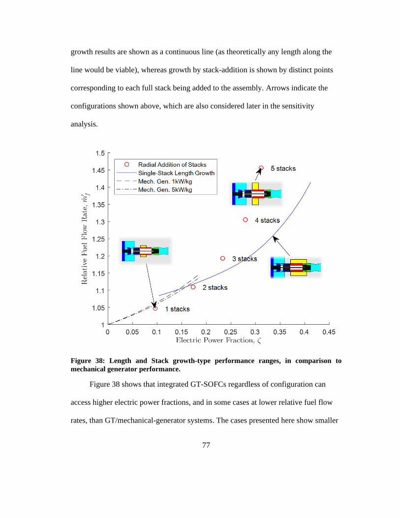
77
growth results are shown as a continuous line (as theoretically any length along the
line would be viable), whereas growth by stack-addition is shown by distinct points
corresponding to each full stack being added to the assembly. Arrows indicate the
configurations shown above, which are also considered later in the sensitivity
analysis.
Figure 38: Length and Stack growth-type performance ranges, in comparison to
mechanical generator performance.
Figure 38 shows that integrated GT-SOFCs regardless of configuration can
access higher electric power fractions, and in some cases at lower relative fuel flow
rates, than GT/mechanical-generator systems. The cases presented here show smaller
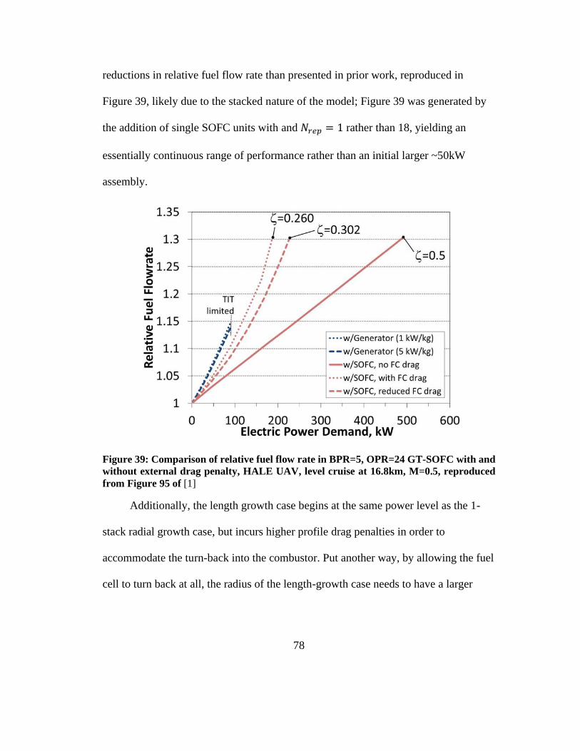
78
reductions in relative fuel flow rate than presented in prior work, reproduced in
Figure 39, likely due to the stacked nature of the model; Figure 39 was generated by
the addition of single SOFC units with and 𝑁𝑟𝑒𝑝 = 1 rather than 18, yielding an
essentially continuous range of performance rather than an initial larger ~50kW
assembly.
Figure 39: Comparison of relative fuel flow rate in BPR=5, OPR=24 GT-SOFC with and
without external drag penalty, HALE UAV, level cruise at 16.8km, M=0.5, reproduced
from Figure 95 of [1]
Additionally, the length growth case begins at the same power level as the 1-
stack radial growth case, but incurs higher profile drag penalties in order to
accommodate the turn-back into the combustor. Put another way, by allowing the fuel
cell to turn back at all, the radius of the length-growth case needs to have a larger
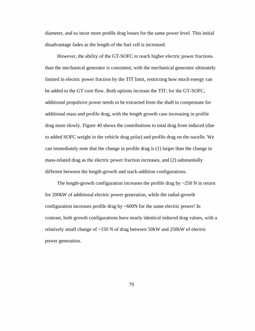
79
diameter, and so incur more profile drag losses for the same power level. This initial
disadvantage fades as the length of the fuel cell is increased.
However, the ability of the GT-SOFC to reach higher electric power fractions
than the mechanical generator is consistent, with the mechanical generator ultimately
limited in electric power fraction by the TIT limit, restricting how much energy can
be added to the GT core flow. Both options increase the TIT; for the GT-SOFC,
additional propulsive power needs to be extracted from the shaft to compensate for
additional mass and profile drag, with the length growth case increasing in profile
drag more slowly. Figure 40 shows the contributions to total drag from induced (due
to added SOFC weight in the vehicle drag polar) and profile drag on the nacelle. We
can immediately note that the change in profile drag is (1) larger than the change in
mass-related drag as the electric power fraction increases, and (2) substantially
different between the length-growth and stack-addition configurations.
The length-growth configuration increases the profile drag by ~250 N in return
for 200kW of additional electric power generation, while the radial-growth
configuration increases profile drag by ~600N for the same electric power! In
contrast, both growth configurations have nearly identical induced drag values, with a
relatively small change of ~150 N of drag between 50kW and 250kW of electric
power generation.
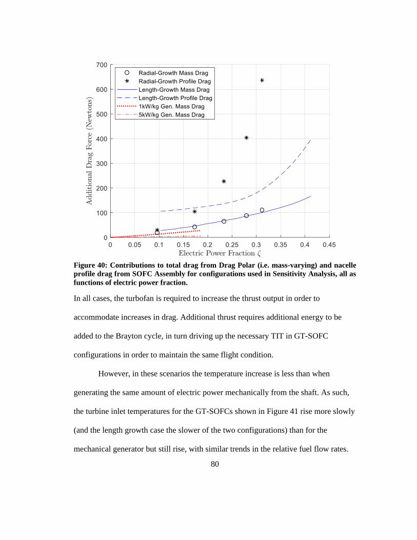
80
Figure 40: Contributions to total drag from Drag Polar (i.e. mass-varying) and nacelle
profile drag from SOFC Assembly for configurations used in Sensitivity Analysis, all as
functions of electric power fraction.
In all cases, the turbofan is required to increase the thrust output in order to
accommodate increases in drag. Additional thrust requires additional energy to be
added to the Brayton cycle, in turn driving up the necessary TIT in GT-SOFC
configurations in order to maintain the same flight condition.
However, in these scenarios the temperature increase is less than when
generating the same amount of electric power mechanically from the shaft. As such,
the turbine inlet temperatures for the GT-SOFCs shown in Figure 41 rise more slowly
(and the length growth case the slower of the two configurations) than for the
mechanical generator but still rise, with similar trends in the relative fuel flow rates.
81
Ultimately, the GT-SOFC systems are restricted by the given spatial constraints rather
than TIT.
Figure 41: Turbine Inlet Temperature Variation with Electric Power Fraction for various
electricity generation configurations on the HALE aircraft model
The increase in TIT implies an increase in throttle setting, with the aircraft here
assumed during design (with no additional electricity generated) to be operating at
60% throttle in cruise. Consequently, an advantage that GT-SOFCs provide is a
greater margin to increase engine throttle than when using mechanical generators for
a given production of electric power.
The overall implication is that efficient aerodynamics for an integrated GT-
SOFC are important for minimizing fuel expenses. Based on the evidence shown
here, the aerodynamics are a more important consideration than the additional mass
82
of the SOFC. Put another way, the power density can be more important than the
specific power if the assembly extends into the airflow.
9.7 Model Uncertainty
For any complicated nonlinear model such as the NPSS modeling performed
here, there is a concern that uncertainties in the input parameters could lead to
uncertainties in the conclusions that the model provides—in this case, that the
uncertainty in fuel flow rate may encompass any variations we observe. This is
checked by multiplying each sensitivity coefficient by the expected uncertainty in its
associated parameter and summing the results in a root-sum-square (RSS) manner to
get an overall uncertainty in fuel flow rate, as shown in Equation (27). Here, 𝑢�̇�𝑓,𝑅𝑆𝑆
is the expected (RSS) uncertainty in fuel flow rate, 𝑢𝑦𝑖 is the uncertainty of any
particular input parameter 𝑦𝑖, 𝑠𝑖 is the sensitivity of the system to that input
parameter, and 𝑁 is the number of parameters considered. Waters and Cadou.[17]
performed a similar analysis but for a smaller set of parameters.
𝑢�̇�𝑓,𝑅𝑆𝑆 = √∑(𝑢𝑦𝑖𝑠𝑖)2
𝑖=𝑁
𝑖=1
(27)
In order to determine the set of sensitivity values 𝑠𝑖, a sensitivity analysis is
performed for each of the converged states for the NPSS GT-SOFC model design
conditions shown in Figure 37. To determine a sensitivity coefficient for each
83
variable in a design condition, the electrical power generated is added to the list of
dependent variables so that the GT-SOFC “performance” of flight condition and
electrical power output can be maintained while our variable of interest is changed. In
order to maintain equal numbers of dependents and independents, the variable 𝑁𝑟𝑒𝑝 is
added to the set of independents for the solver, allowing the size of the fuel cell stacks
used to vary slightly to accommodate fractional changes in the variables of interest by
providing slightly more or less reacting surface area in the SOFC. A finite difference
method is used to estimate 𝜕�̇�𝑓 𝜕𝑦𝑖⁄ is generated by slightly increasing or decreasing
the value of the property 𝑦𝑖 and re-calculating �̇�𝑓. The amount of increase/decrease
is ~5% and is chosen as needed in order to cause changes in excess of the solver
tolerances. The value of 𝑦𝑖 is re-set and the solver is then run again to check
convergence back to the original conditions. Equation (28) gives the formula for the
sensitivity of �̇�𝑓 to the ith parameter.
𝑠𝑖 = (�̇�𝑓,𝑖 − �̇�𝑓,0)/Δy𝑖 (28)
Figure 42 shows the sensitivity of �̇�𝑓 to various parameters in the HALE
aircraft operating at 55kft and M=0.5 for the three different designs illustrated in
Figure 37.
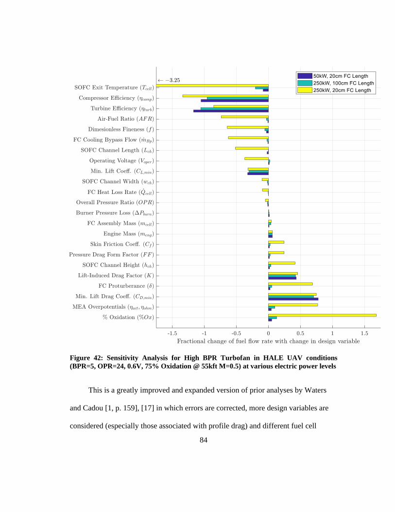
84
Figure 42: Sensitivity Analysis for High BPR Turbofan in HALE UAV conditions
(BPR=5, OPR=24, 0.6V, 75% Oxidation @ 55kft M=0.5) at various electric power levels
This is a greatly improved and expanded version of prior analyses by Waters
and Cadou [1, p. 159], [17] in which errors are corrected, more design variables are
considered (especially those associated with profile drag) and different fuel cell

85
configurations are considered. In particular, the determination of turbomachinery
efficiency (𝜂𝑡𝑢𝑟𝑏 , 𝜂𝑐𝑜𝑚𝑝) sensitivity has been corrected, and sensitivities to an
additional drag polar variable (𝐶𝐿,𝑚𝑖𝑛) and fuel cell profile drag variables
(𝐶𝑓 , 𝑓, 𝐹𝐹, 𝛿) have been included. Different power levels are also considered to
illustrate the importance of making comparisons at different electric power fractions.
The higher operating voltage of 0.7V with 90% conversion of fuel described in
previous work has been omitted as any performance improvement is generally lower
than the case given here. This is borne out by the lower sensitivity to operating
voltage compared to the degree of oxidation which indicates an increasing fuel flow
rate as higher conversions are targeted.
The most striking conclusion from the updated sensitivity analysis is that the
flow-occluding configuration (adding stacks radially to add electric power rather than
lengthening the existing fuel cells) yields order-of-magnitude greater sensitivities for
values related to the fuel cell subsystem than either the lower power level or length-
growth configuration at the same higher power level, with the most extreme
sensitivity being to the SOFC exit temperature: Every 1% increase of fuel cell
operating temperature reduces the relative fuel flow rate by over 3%!
As further evidence, all SOFC-related variables indicate reductions in the fuel
flow rate by reducing the mass and especially profile drag of the system. For
example, an increase in SOFC operating temperature increases the power density of
the SOFC, allowing for a smaller fuel cell (in this case one with a lower 𝑁𝑟𝑒𝑝) to
provide the same target power level.

86
Finally, the sensitivity to variables unrelated to the SOFC assembly are only
somewhat altered between all three cases tested, despite the difference in electric
power generation and relative fuel flow rates observed. For all tested variables, a brief
narrative explanation the system’s sensitivity to each variable is provided in Table 5.
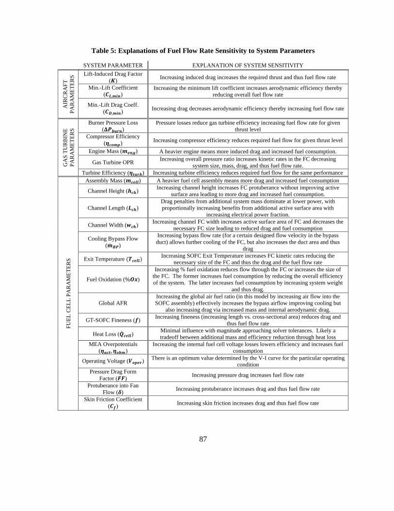
87
Table 5: Explanations of Fuel Flow Rate Sensitivity to System Parameters
SYSTEM PARAMETER EXPLANATION OF SYSTEM SENSITIVITY A
IRC
RA
FT
PA
RA
ME
TE
RS
Lift-Induced Drag Factor
(𝑲) Increasing induced drag increases the required thrust and thus fuel flow rate
Min.-Lift Coefficient
(𝑪𝑳,𝒎𝒊𝒏) Increasing the minimum lift coefficient increases aerodynamic efficiency thereby
reducing overall fuel flow rate
Min.-Lift Drag Coeff.
(𝑪𝑫,𝒎𝒊𝒏) Increasing drag decreases aerodynamic efficiency thereby increasing fuel flow rate
GA
S T
UR
BIN
E
PA
RA
ME
TE
RS
Burner Pressure Loss
(𝚫𝑷𝒃𝒖𝒓𝒏)
Pressure losses reduce gas turbine efficiency increasing fuel flow rate for given
thrust level
Compressor Efficiency
(𝜼𝒄𝒐𝒎𝒑) Increasing compressor efficiency reduces required fuel flow for given thrust level
Engine Mass (𝒎𝒆𝒏𝒈) A heavier engine means more induced drag and increased fuel consumption.
Gas Turbine OPR Increasing overall pressure ratio increases kinetic rates in the FC decreasing
system size, mass, drag, and thus fuel flow rate.
Turbine Efficiency (𝜼𝒕𝒖𝒓𝒃) Increasing turbine efficiency reduces required fuel flow for the same performance
FU
EL
CE
LL
PA
RA
ME
TE
RS
Assembly Mass (𝒎𝒄𝒆𝒍𝒍) A heavier fuel cell assembly means more drag and increased fuel consumption
Channel Height (𝒉𝒄𝒉) Increasing channel height increases FC protuberance without improving active
surface area leading to more drag and increased fuel consumption.
Channel Length (𝑳𝒄𝒉)
Drag penalties from additional system mass dominate at lower power, with
proportionally increasing benefits from additional active surface area with
increasing electrical power fraction.
Channel Width (𝒘𝒄𝒉) Increasing channel FC width increases active surface area of FC and decreases the
necessary FC size leading to reduced drag and fuel consumption
Cooling Bypass Flow
(�̇�𝑩𝑷)
Increasing bypass flow rate (for a certain designed flow velocity in the bypass
duct) allows further cooling of the FC, but also increases the duct area and thus
drag
Exit Temperature (𝑻𝒄𝒆𝒍𝒍) Increasing SOFC Exit Temperature increases FC kinetic rates reducing the
necessary size of the FC and thus the drag and the fuel flow rate
Fuel Oxidation (%𝑶𝒙)
Increasing % fuel oxidation reduces flow through the FC or increases the size of
the FC. The former increases fuel consumption by reducing the overall efficiency
of the system. The latter increases fuel consumption by increasing system weight
and thus drag.
Global AFR
Increasing the global air fuel ratio (in this model by increasing air flow into the
SOFC assembly) effectively increases the bypass airflow improving cooling but
also increasing drag via increased mass and internal aerodynamic drag.
GT-SOFC Fineness (𝒇) Increasing fineness (increasing length vs. cross-sectional area) reduces drag and
thus fuel flow rate
Heat Loss (�̇�𝒄𝒆𝒍𝒍) Minimal influence with magnitude approaching solver tolerances. Likely a
tradeoff between additional mass and efficiency reduction through heat loss
MEA Overpotentials
(𝜼𝒂𝒄𝒕, 𝜼𝒐𝒉𝒎)
Increasing the internal fuel cell voltage losses lowers efficiency and increases fuel
consumption
Operating Voltage (𝑽𝒐𝒑𝒆𝒓) There is an optimum value determined by the V-I curve for the particular operating
condition
Pressure Drag Form
Factor (𝑭𝑭) Increasing pressure drag increases fuel flow rate
Protuberance into Fan
Flow (𝜹) Increasing protuberance increases drag and thus fuel flow rate
Skin Friction Coefficient
(𝑪𝒇) Increasing skin friction increases drag and thus fuel flow rate
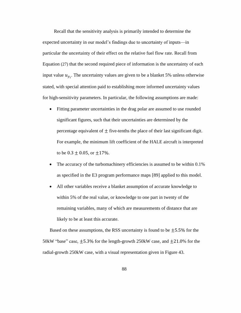
88
Recall that the sensitivity analysis is primarily intended to determine the
expected uncertainty in our model’s findings due to uncertainty of inputs—in
particular the uncertainty of their effect on the relative fuel flow rate. Recall from
Equation (27) that the second required piece of information is the uncertainty of each
input value 𝑢𝑦𝑖. The uncertainty values are given to be a blanket 5% unless otherwise
stated, with special attention paid to establishing more informed uncertainty values
for high-sensitivity parameters. In particular, the following assumptions are made:
• Fitting parameter uncertainties in the drag polar are assumed to use rounded
significant figures, such that their uncertainties are determined by the
percentage equivalent of ± five-tenths the place of their last significant digit.
For example, the minimum lift coefficient of the HALE aircraft is interpreted
to be 0.3 ± 0.05, or ±17%.
• The accuracy of the turbomachinery efficiencies is assumed to be within 0.1%
as specified in the E3 program performance maps [89] applied to this model.
• All other variables receive a blanket assumption of accurate knowledge to
within 5% of the real value, or knowledge to one part in twenty of the
remaining variables, many of which are measurements of distance that are
likely to be at least this accurate.
Based on these assumptions, the RSS uncertainty is found to be ±5.5% for the
50kW “base” case, ±5.3% for the length-growth 250kW case, and ±21.0% for the
radial-growth 250kW case, with a visual representation given in Figure 43.
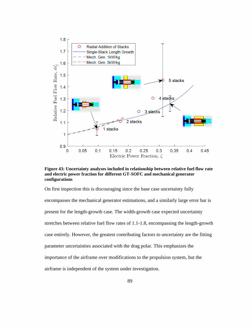
89
Figure 43: Uncertainty analyses included in relationship between relative fuel flow rate
and electric power fraction for different GT-SOFC and mechanical generator
configurations
On first inspection this is discouraging since the base case uncertainty fully
encompasses the mechanical generator estimations, and a similarly large error bar is
present for the length-growth case. The width-growth case expected uncertainty
stretches between relative fuel flow rates of 1.1-1.8, encompassing the length-growth
case entirely. However, the greatest contributing factors to uncertainty are the fitting
parameter uncertainties associated with the drag polar. This emphasizes the
importance of the airframe over modifications to the propulsion system, but the
airframe is independent of the system under investigation.
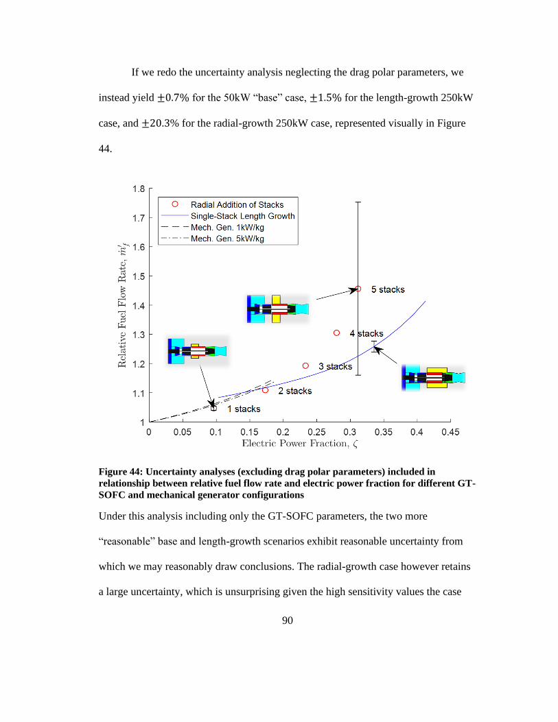
90
If we redo the uncertainty analysis neglecting the drag polar parameters, we
instead yield ±0.7% for the 50kW “base” case, ±1.5% for the length-growth 250kW
case, and ±20.3% for the radial-growth 250kW case, represented visually in Figure
44.
Figure 44: Uncertainty analyses (excluding drag polar parameters) included in
relationship between relative fuel flow rate and electric power fraction for different GT-
SOFC and mechanical generator configurations
Under this analysis including only the GT-SOFC parameters, the two more
“reasonable” base and length-growth scenarios exhibit reasonable uncertainty from
which we may reasonably draw conclusions. The radial-growth case however retains
a large uncertainty, which is unsurprising given the high sensitivity values the case

91
had for many fuel-cell parameters. The conclusion is that this questionably physical
case likely stretches the pylon drag model beyond its region of usability.
In closing, it has been shown here that profile drag may constitute a
substantial barrier to minimizing the relative fuel flow rate for GT-SOFC systems,
usually well in excess of mass-induced drag penalties. Additionally, we may conclude
that while a GT-SOFC has an increasing improvement versus a mechanical generator
at higher electric power fractions, the most significant advantage is in generating
greater amounts of electrical power before encountering the turbine inlet temperature
limit.
92
10 APU Model
10.1 Approach
The Ultra/AMI D300 (Figure 45) is a propane-fueled, SOFC-based APU that
produces 300W (32V, 9.5A). It is similar to the current D300 and was marketed to
the US military primarily for the purpose of recharging batteries in the field
quietly.[63], [90]
Figure 45: Two Ultra/AMI D300 APUs with standard propane tank supply
The APU features a set of 56 tubular, propane-fueled SOFCs each with an integrated
CPOx fuel reformer that converts the propane fuel to syngas (predominantly H2 and
CO) for use by the fuel cell. The tubular cells are bundled together in a cylindrical array
with a CPOx reformer making up roughly the front third on the upstream side of each
tube followed by SOFC in the remaining two-thirds. Immediately downstream of the
SOFC array is a combustor that burns the remaining fuel and oxidizer to maintain

93
system temperature. The integrated CPOx/SOFC element is shown in Figure 46. Its
compact, self-contained nature makes it very well suited for integrating with a small
gas turbine: It has a single air inlet, a single exhaust outlet, built-in instrumentation
that measures air and fuel flow rates as well as temperatures and currents in all of the
FC elements, and its own control system. The initial plan is to retain the control system
and continue to operate on propane. Subsequent efforts would replace the control
system and switch the fuel to Jet-A.
While the APU is designed to operate at approximately 1 atm of pressure, the
manufacturer has indicated that it is possible to operate it at higher pressures - albeit at
higher risks of leaking and overheating. The manufacturer has also indicated that the
reformer would likely work with Jet-A for some unknown period.
Note from Figure 46 that the main power generation components only occupy
the bottom half of the APU. The rest of the space is taken up by fuel filtering, battery,
power electronics, and blowers. This illustrates the significant effect that balance-of-
plant components have on the mass and volume of fuel cell systems. Note also the
similar size of the APU compared to the small gas turbine whose power output is well
in excess of 10 kW, constituting greater than an order of magnitude greater power
density over the APU. This demonstrates the power density advantage of engine-based
energy conversion systems over unhybridized fuel-cell-based energy conversion
systems.
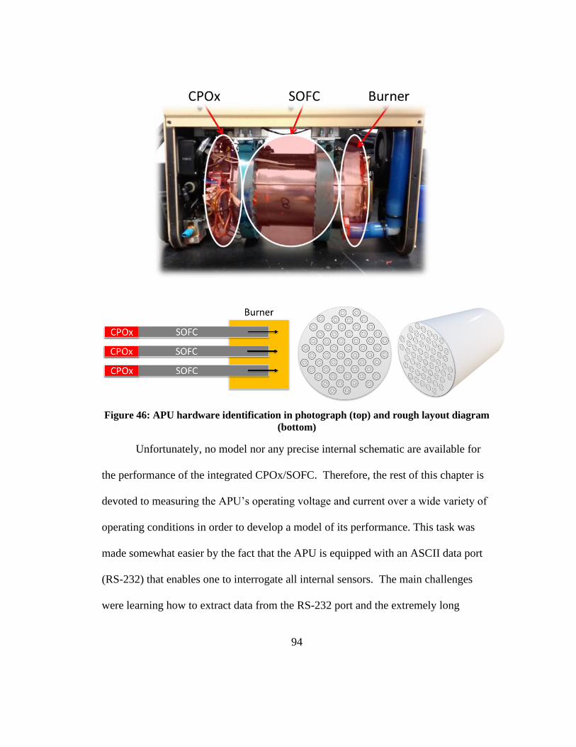
94
Figure 46: APU hardware identification in photograph (top) and rough layout diagram
(bottom)
Unfortunately, no model nor any precise internal schematic are available for
the performance of the integrated CPOx/SOFC. Therefore, the rest of this chapter is
devoted to measuring the APU’s operating voltage and current over a wide variety of
operating conditions in order to develop a model of its performance. This task was
made somewhat easier by the fact that the APU is equipped with an ASCII data port
(RS-232) that enables one to interrogate all internal sensors. The main challenges
were learning how to extract data from the RS-232 port and the extremely long

95
equilibration time of the system which eventually required the development of
methods for inferring steady-state performance from non-steady-state measurements.
What follows are the results of a non-destructive characterization of the
system. From here onward, I will refer to ‘measurements’, ‘data points’, ‘operating
conditions’, ‘runs’ and ‘experiments’. ‘Measurements’ will refer to raw data output
from the device while ‘data points’ refers to the processed results of those
measurements to generate a single value for a given operating condition. An
‘operating condition’ is a set state of operation for the system for which we are trying
to generate a data point. A ‘run’ refers to a physical instance of data collection using
the standard operating procedure discussed later in this chapter, while an ‘experiment’
is the collection process for a single data point.
10.2 Instrumentation and Data Acquisition
Conveniently, the APU is instrumented with a variety of temperature, flow
rate, and other status sensors placed at a variety of locations within the housing to
inform the control system of the APU status. Less conveniently, almost all of these
sensors are inaccessible for calibration, knowledge of precise location, and
replacement without disassembling the device. Furthermore, this makes connecting
additional external instrumentation difficult and calibration nearly impossible without
substantial risk of damaging the system.
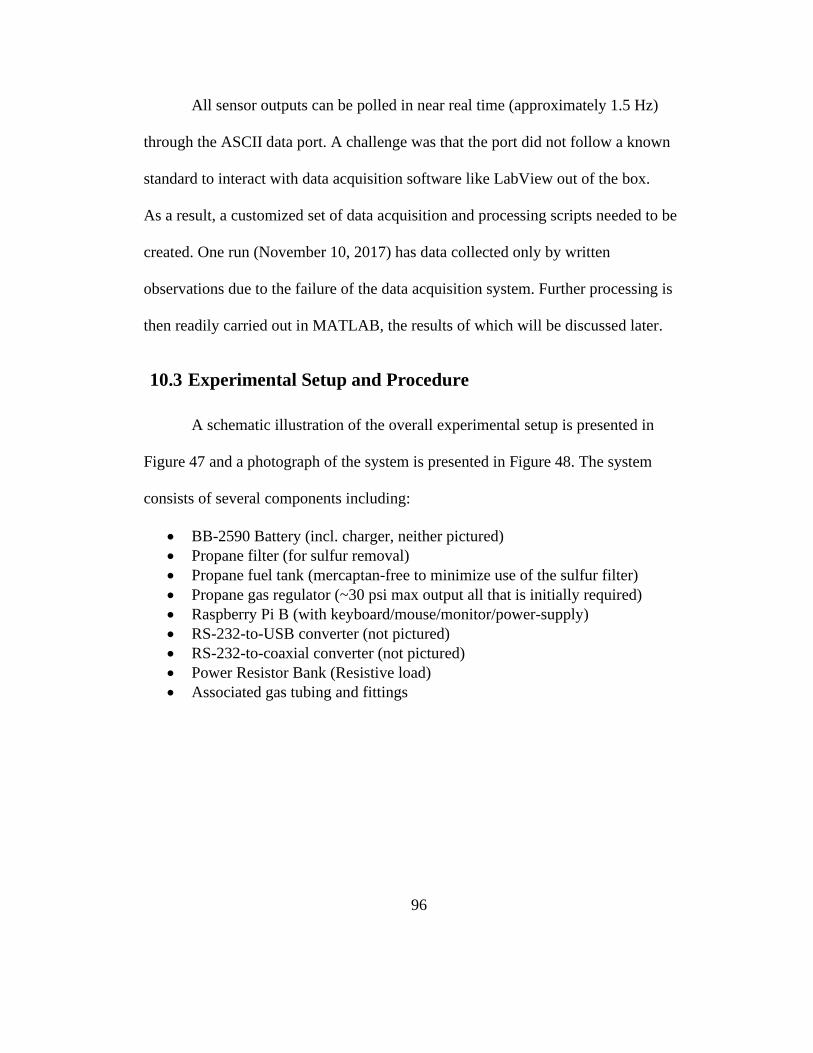
96
All sensor outputs can be polled in near real time (approximately 1.5 Hz)
through the ASCII data port. A challenge was that the port did not follow a known
standard to interact with data acquisition software like LabView out of the box.
As a result, a customized set of data acquisition and processing scripts needed to be
created. One run (November 10, 2017) has data collected only by written
observations due to the failure of the data acquisition system. Further processing is
then readily carried out in MATLAB, the results of which will be discussed later.
10.3 Experimental Setup and Procedure
A schematic illustration of the overall experimental setup is presented in
Figure 47 and a photograph of the system is presented in Figure 48. The system
consists of several components including:
• BB-2590 Battery (incl. charger, neither pictured)
• Propane filter (for sulfur removal)
• Propane fuel tank (mercaptan-free to minimize use of the sulfur filter)
• Propane gas regulator (~30 psi max output all that is initially required)
• Raspberry Pi B (with keyboard/mouse/monitor/power-supply)
• RS-232-to-USB converter (not pictured)
• RS-232-to-coaxial converter (not pictured)
• Power Resistor Bank (Resistive load)
• Associated gas tubing and fittings
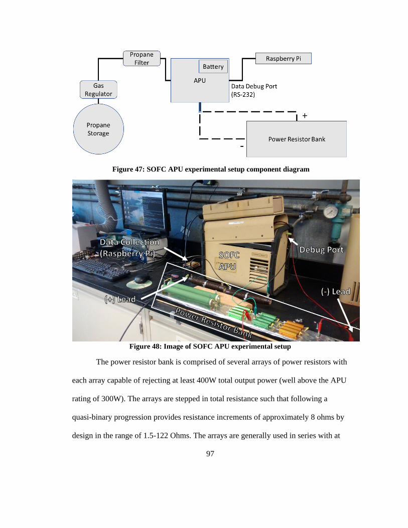
97
Figure 48: Image of SOFC APU experimental setup
The power resistor bank is comprised of several arrays of power resistors with
each array capable of rejecting at least 400W total output power (well above the APU
rating of 300W). The arrays are stepped in total resistance such that following a
quasi-binary progression provides resistance increments of approximately 8 ohms by
design in the range of 1.5-122 Ohms. The arrays are generally used in series with at
Figure 47: SOFC APU experimental setup component diagram

98
least one 1.5Ω 400W dissipation-rated power resistors connected at all times for
safety. Clip leads connect the power output terminals inside the APU body to the load
bank. The negative lead is connected to a safety switch that is turned off before
changing the load state. Cooling is provided by a room fan that blows air along the
length of the power resistor bank, starting near the negative lead. The resistive load
applied to the APU is changed by connecting and disconnecting different sets of
power resistors at clip connections shown in Figure 49. Each set of power resistors is
rated to handle 400W of dissipation in series, though in nearly all scenarios this is a
substantial safety margin since the APU is rated to 300W maximum output, and the
internal power conditioning causes it to function as a constant-voltage source of
32.6V that limits the power dissipation to 𝑃 = 𝑉2/𝑅, or 𝑃 = 1063/𝑅. If the given
300W output is to be followed, the lower boundary for the resistance value is
approximately 4Ω, while any higher resistance value will be dissipating less power.
While the stack voltage may exceed the output voltage at low current values, in the
case of a short the stack supply voltage would drop precipitously, again lowering the
effective power output. Practically, individual resistors within the sets may be placed
in series or parallel (e.g. two 2Ω resistors in parallel yielding a single ohm) to achieve
greater resolution of resistance when their individual power dissipation ratings will
not be exceeded in the overall circuit. The varied load allows us to access a range of
operating points along the stack potential curve, albeit generating a nonlinear range of
power. This can be seen in Table 6 which is a partial (of a total of 64 design states)
state table assuming that the APU output remains constant at 32.6V (std. deviation ≈
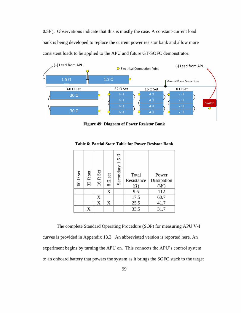
99
0.5𝑉). Observations indicate that this is mostly the case. A constant-current load
bank is being developed to replace the current power resistor bank and allow more
consistent loads to be applied to the APU and future GT-SOFC demonstrator.
Figure 49: Diagram of Power Resistor Bank
Table 6: Partial State Table for Power Resistor Bank
60 Ω
set
32 Ω
set
16 Ω
Set
8 Ω
set
Sec
ondar
y 1
.5 Ω
Total
Resistance
(Ω)
Power
Dissipation
(𝑊) X 9.5 112
X 17.5 60.7
X X 25.5 41.7
X 33.5 31.7
The complete Standard Operating Procedure (SOP) for measuring APU V-I
curves is provided in Appendix 13.3. An abbreviated version is reported here. An
experiment begins by turning the APU on. This connects the APU’s control system
to an onboard battery that powers the system as it brings the SOFC stack to the target

100
operating temperature of 790 C. Once this temperature is reached, the control system
switches to electrical power generated by the SOFC and recharges the battery. Our
experiments begin after the battery is recharged (approximately one hour) and the
system has reached equilibrium. It takes an additional 20-30 for the system to
equilibrate between operating conditions. When a set of experiments is complete,
the system proceeds with an approximately 20 to 30 minute shutdown sequence
where the fuel cell is allowed to cool slowly. This is likely to prevent system damage
from mechanical stresses induced by coefficient of thermal expansion (CTE)
mismatch to the tubular cell, as well as to the Nickel anode, which can degrade at
high temperatures under oxygen or water to form NiO. The formation of bulk NiO
places substantial mechanical stresses on the anode layer and can permanently
damage the performance of the SOFC.[82], [91] Similarly to prevent unwanted
oxidation of the anode, it has been suggested to operate the SOFC at cell voltages
greater than 0.6V, which in this system indicates a stack voltage of 33.6V. This is all
in addition to dangers of rapid or uneven thermal contraction. In some instances, the
APU has suddenly lost power and turned off without this shutdown cycle. If this
happens, it is important to rapidly restart the system and resume the controlled
shutdown cycle in order to prevent damage. The system provides no notification of
power failure; consequently, the power loss has not always been noted immediately
and the system has been allowed to stand hot for at most the length of an experiment
(~20-30 minutes). However, such instances are not correlated to the varying
polarization curve provided by the APU shown in later sections.

101
The goal of the experiments is to measure the SOFC’s polarization (V-I) curve
by varying the electrical load on the system and measuring V and I. All results are for
a single stack operating temperature (790C) because of the control system. Future
experiments could investigate the effect of changing the target operating temperature
(by bypassing the control system) and increasing the operating pressure (by feeding
the stack compressed air).
10.4 Typical Data and Challenges
While it would be tedious to display all sensor outputs, several are of
importance and will be illustrated as they appear in a test run with a single trial. Most
important are the “stack” voltage and current values which measure the state of the
fuel cell stack itself, rather than the operating output of the APU system, which
includes substantial power conditioning and balance-of-plant losses that are distinct
from the CPOx/SOFC.
Other important variables include the stack temperatures, and flow rates. The APU
operates at local atmospheric pressure. Figure 50 below shows time histories of
voltages, currents, power output, temperatures, and flow rates over the course of a
single run from start to finish. This particular run included only one load point which
was the recharging of the starter battery.
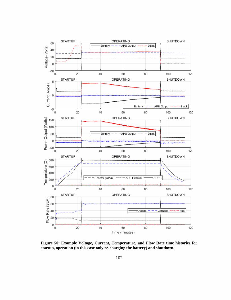
102
Figure 50: Example Voltage, Current, Temperature, and Flow Rate time histories for
startup, operation (in this case only re-charging the battery) and shutdown.

103
Figure 50 also shows startup and shutdown conditions. During startup, the
onboard battery is used to start the system balance of plant for approximately 25
minutes. During this period, the SOFC stack is not under load, and its voltage rises to
nearly the open-circuit voltage (OCV) before the system switches from the battery to
the SOFC stack to maintain balance of plant. The stack voltage just prior to the
startup of each run lacks the balance-of-plant loads and has temperature conditions
closest (within approximately 5K of the operating temperature) to those during
operation. As such, it can be considered the OCV of the stack, usually observed to be
around 0.9V. The current draw from the battery during startup is substantial: over an
amp (at ~16.5V from two batteries). Fuel and air burned in the tail gas combustor
heats cathode air raising the temperature of the SOFC
When the SOFC reaches its target temperature (790C), the system switches
from battery power to SOFC power and recharges the battery. The charging current
tapers off as the battery approaches capacity although charging will continue at
trickle-charge levels. Temperatures, the APU output voltage, and fuel and air flow
rates generally remain stable during operation although the actual demands on the
SOFC will vary with load and charge condition of the battery.
During shutdown, fuel and anode flow (a partial oxidation of fuel and air) will
cease while airflow through the cathode continues. The SOFC stack is disconnected
from both internal and external loads while the recharged battery resumes powering
the balance of plant. The CPOx/SOFC cool steadily during shutdown until a
sufficiently low temperature (~150 C) is reached that the system can be shut down. In
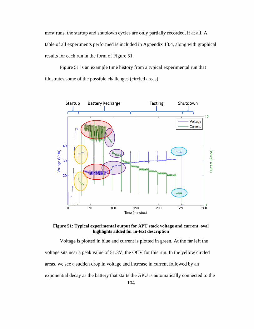
104
most runs, the startup and shutdown cycles are only partially recorded, if at all. A
table of all experiments performed is included in Appendix 13.4, along with graphical
results for each run in the form of Figure 51.
Figure 51 is an example time history from a typical experimental run that
illustrates some of the possible challenges (circled areas).
Figure 51: Typical experimental output for APU stack voltage and current, oval
highlights added for in-text description
Voltage is plotted in blue and current is plotted in green. At the far left the
voltage sits near a peak value of 51.3V, the OCV for this run. In the yellow circled
areas, we see a sudden drop in voltage and increase in current followed by an
exponential decay as the battery that starts the APU is automatically connected to the

105
system and subsequently recharged. The battery is allowed to fully charge before
measurements are collected.
The red ovals above (second from left) show the response of the system to an
overload condition when more current is demanded than is considered ‘safe’ by the
control system. The protection mode causes ‘noisy’ data as the load is rapidly
disconnected and reconnected by the control system. This protection mode prevents
access to the full SOFC polarization curve by setting an upper limit on current and a
corresponding lower limit on voltage.
The purple ovals show the temporal responses of voltage and current to the
application of a fixed resistive load. Voltage and current oscillate, likely due to
control system feedback, while the averages approach steady-state asymptotically.
It can take 20-30 minutes or even longer (according to the manufacturer) to reach
equilibrium. This is a significant problem because it makes experiments take a long
time and makes it hard to know when the system has really reached equilibrium.
Strategies for predicting voltage and current at equilibrium by fitting curves to time
histories are addressed in a later section.
Finally, the rightmost set of blue ovals show voltage and current time histories
associated with no external load connected. Current is not zero and voltage is not near
the maximum observed (51.3V as the observed OCV) because of the balance of plant
loads. This prevents us from measuring the low-current/ high-voltage portions of the
polarization curve. While some insight might be gained from the response of the
system under battery power as the fuel cell comes up to temperature during startup,
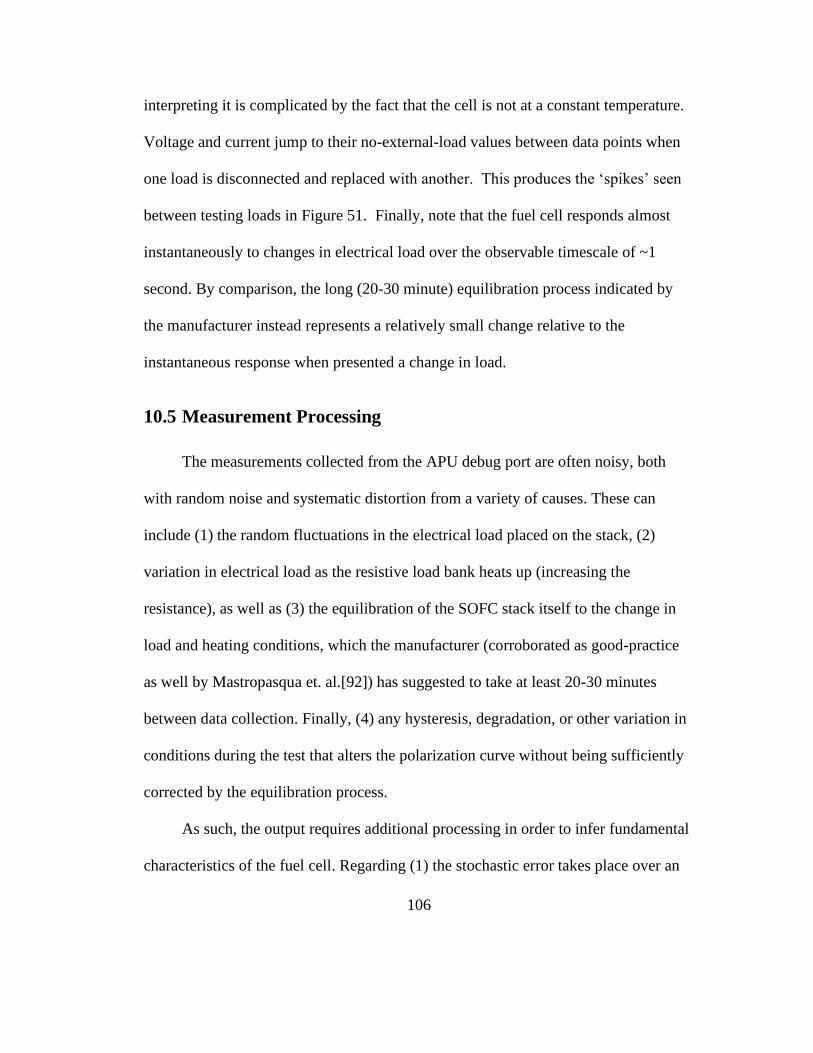
106
interpreting it is complicated by the fact that the cell is not at a constant temperature.
Voltage and current jump to their no-external-load values between data points when
one load is disconnected and replaced with another. This produces the ‘spikes’ seen
between testing loads in Figure 51. Finally, note that the fuel cell responds almost
instantaneously to changes in electrical load over the observable timescale of ~1
second. By comparison, the long (20-30 minute) equilibration process indicated by
the manufacturer instead represents a relatively small change relative to the
instantaneous response when presented a change in load.
10.5 Measurement Processing
The measurements collected from the APU debug port are often noisy, both
with random noise and systematic distortion from a variety of causes. These can
include (1) the random fluctuations in the electrical load placed on the stack, (2)
variation in electrical load as the resistive load bank heats up (increasing the
resistance), as well as (3) the equilibration of the SOFC stack itself to the change in
load and heating conditions, which the manufacturer (corroborated as good-practice
as well by Mastropasqua et. al.[92]) has suggested to take at least 20-30 minutes
between data collection. Finally, (4) any hysteresis, degradation, or other variation in
conditions during the test that alters the polarization curve without being sufficiently
corrected by the equilibration process.
As such, the output requires additional processing in order to infer fundamental
characteristics of the fuel cell. Regarding (1) the stochastic error takes place over an
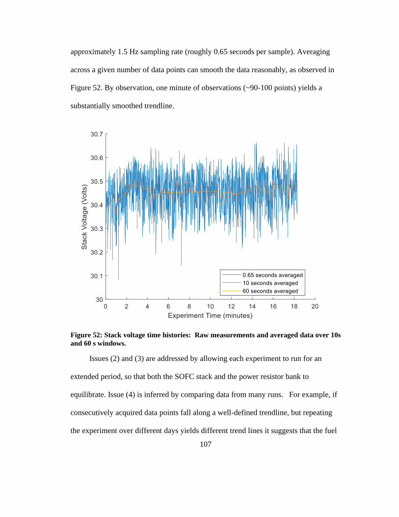
107
approximately 1.5 Hz sampling rate (roughly 0.65 seconds per sample). Averaging
across a given number of data points can smooth the data reasonably, as observed in
Figure 52. By observation, one minute of observations (~90-100 points) yields a
substantially smoothed trendline.
Figure 52: Stack voltage time histories: Raw measurements and averaged data over 10s
and 60 s windows.
Issues (2) and (3) are addressed by allowing each experiment to run for an
extended period, so that both the SOFC stack and the power resistor bank to
equilibrate. Issue (4) is inferred by comparing data from many runs. For example, if
consecutively acquired data points fall along a well-defined trendline, but repeating
the experiment over different days yields different trend lines it suggests that the fuel
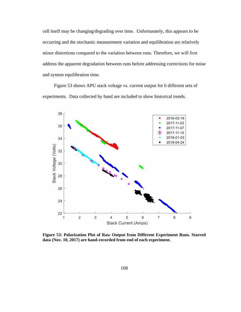
108
cell itself may be changing/degrading over time. Unfortunately, this appears to be
occurring and the stochastic measurement variation and equilibration are relatively
minor distortions compared to the variation between runs. Therefore, we will first
address the apparent degradation between runs before addressing corrections for noise
and system equilibration time.
Figure 53 shows APU stack voltage vs. current output for 6 different sets of
experiments. Data collected by hand are included to show historical trends.
Figure 53: Polarization Plot of Raw Output from Different Experiment Runs. Starred
data (Nov. 10, 2017) are hand-recorded from end of each experiment.
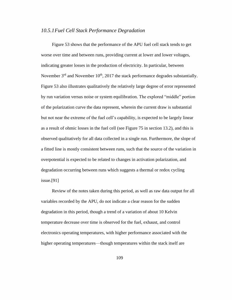
109
10.5.1 Fuel Cell Stack Performance Degradation
Figure 53 shows that the performance of the APU fuel cell stack tends to get
worse over time and between runs, providing current at lower and lower voltages,
indicating greater losses in the production of electricity. In particular, between
November 3rd and November 10th, 2017 the stack performance degrades substantially.
Figure 53 also illustrates qualitatively the relatively large degree of error represented
by run variation versus noise or system equilibration. The explored “middle” portion
of the polarization curve the data represent, wherein the current draw is substantial
but not near the extreme of the fuel cell’s capability, is expected to be largely linear
as a result of ohmic losses in the fuel cell (see Figure 75 in section 13.2), and this is
observed qualitatively for all data collected in a single run. Furthermore, the slope of
a fitted line is mostly consistent between runs, such that the source of the variation in
overpotential is expected to be related to changes in activation polarization, and
degradation occurring between runs which suggests a thermal or redox cycling
issue.[91]
Review of the notes taken during this period, as well as raw data output for all
variables recorded by the APU, do not indicate a clear reason for the sudden
degradation in this period, though a trend of a variation of about 10 Kelvin
temperature decrease over time is observed for the fuel, exhaust, and control
electronics operating temperatures, with higher performance associated with the
higher operating temperatures—though temperatures within the stack itself are
110
consistent. Furthermore, sets of runs together before and after November 2017
appear to be internally consistent, i.e. the degradation occurred over a couple of runs,
and has stabilized, which indicates that this may have been some kind of break-in
process for the APU.
A possible explanation for the degradation include the formation of NiO from
Ni in the anode during shutdown.[91] Fuel flow ceases during shutdown, so oxygen
supplied from reacted water and carbon dioxide or air may leak into the anode
chamber provide the oxidative environment. NiO formation places mechanical stress
on the anode material and alters the nickel grain size, amount, and geometry, reducing
the number of active sites in the anode. Alternatively, sulfur impurities could degrade
performance—albeit in this case desulfurized propane (<1ppm) and a sulfur filter
were employed to prevent this effect.
Finally, individual SOFC tubes may have failed (e.g. shorted out), as the system
does not report on the status of each unit within the stack. In fact, the observed open
circuit voltages are approximately 0.9V, which is lower than the 1.1V typically
expected for SOFC systems.[82, p. 1213] This suggests that the overall stack voltage
should be divided between fewer than the total 56 tubular SOFC units present in the
APU, perhaps as many as 10 of the 56 if the typical open circuit voltage is achieved.
However, the OCV value of the stack is largely consistent across all runs (0.91-
0.89V), which is evidence that the observed ~10% degradation isn’t due to additional
SOFC units shorting out.

111
As it represents the current performance of the fuel cell, we can consider the
observed polarization curve to be represented by the data collected on Nov. 10th, 2017
and onward. While other data collected can be used for testing different processing
methods, they do not represent the current polarization curve of this APU unit.
10.5.2 Last Minute Analysis
One strategy for addressing the equilibration problem is to simply wait a
specified amount of time (the same for every new data point) and then average over
the last minute to get a voltage and a current. Figure 54 shows the results of such an
approach, including experiments that were only hand-recorded since they were taken
at the end of each experiment as well.
112
Figure 54: Polarization curve derived from average of last-minute data with one
standard deviation error bars; starred data indicate hand-recorded experiments
without error information
Although difficult to see, the data in Figure 54 also have error bars indicating one
standard deviation in both cell voltage and cell current, which clearly show that the
trend is much larger than the measurement uncertainty. When we limit our results to
the more recent data points (i.e. from Nov.10th 2017 and onwards) and apply a linear
fit, we generate Figure 55. Figure 55 also includes the observed OCV during later
runs, although the intervening low-current region of the polarization curve is
currently inaccessible while the stack is used to maintain the balance of plant in the
APU.
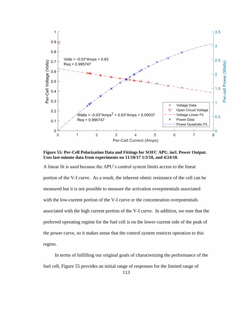
113
Figure 55: Per-Cell Polarization Data and Fittings for SOFC APU, incl. Power Output.
Uses last-minute data from experiments on 11/10/17 1/3/18, and 4/24/18.
A linear fit is used because the APU’s control system limits access to the linear
portion of the V-I curve. As a result, the inherent ohmic resistance of the cell can be
measured but it is not possible to measure the activation overpotentials associated
with the low-current portion of the V-I curve or the concentration overpotentials
associated with the high current portion of the V-I curve. In addition, we note that the
preferred operating regime for the fuel cell is on the lower-current side of the peak of
the power curve, so it makes sense that the control system restricts operation to this
region.
In terms of fulfilling our original goals of characterizing the performance of the
fuel cell, Figure 55 provides an initial range of responses for the limited range of

114
operating parameters available to the un-modified APU. Further characterization will
require disassembly of the APU (to disentangle balance of plant loads from the SOFC
stack) or other equipment such as electronic impedance spectrometry measurements
to clarify different components of the SOFC electrochemistry.
10.6 Improvements for Future Data Collection
The lab-scale gas turbine-APU hybrid will be difficult and expensive to run
for long periods of time which, behooves us to find ways to predict performance at an
operating condition without having to wait for the system to equilibrate fully. While
replacing the load bank with a constant current load could help, it would only do so if
the APU’s equilibration time scale is of similar length or shorter than that of the load
bank. This is unlikely given that the APU is substantially larger than the load bank so
other strategies will likely be required.
10.6.1 Establishing Convergence
For the purposes of investigating the electrochemical properties of GT-SOFC
systems, we need to establish a definition for when the fuel cell stack (and eventually
the entire hybrid system) has reached equilibrium. Considering that without infinite
time we don’t precisely know what the equilibrium condition will be a priori, we
require a practical estimation that will be reasonably close. The simplest method is to
simply allow the SOFC to operate at a single condition for an extended period, but
long operating times are not always feasible.

115
For a given system, we can attempt to establish a reasonable timeframe or rate
of change that, during the run, we can determine a system to be converged ‘close
enough’ to the equilibrium value. The specific means of establishing the rate of
change and/or an appropriate timeframe will depend on the physical size, thermal
mass, and electrochemistry of the system, but for our purposes here will be
determined empirically from the range of data already collected.
Consider Figure 56 which plots the voltage and current time histories
collected from all experiments, with some spurious data omitted. In particular, data
were removed if they were collected while the battery was charging (in this case
defined to be a current load greater than a minute-averaged 0.1 Amp), thus changing
the load over time. We also removed one final spurious experiment which
experienced a temporary reduction in internal load during the run from a change in
demand from the balance of plant.
The remaining time histories are averaged over one minute intervals (as in
Figure 52) and then normalized by the final minute’s data which usually occurs at run
times between 20 and 30 minutes, although some experiments have lasted an hour or
more. The resulting curves show a maximum variation of 1% of voltage and 8% of
current measurements from start to finish for all remaining experiments (Figure 56).
Figure 56 also includes the power output of the stack during all remaining
experiments.
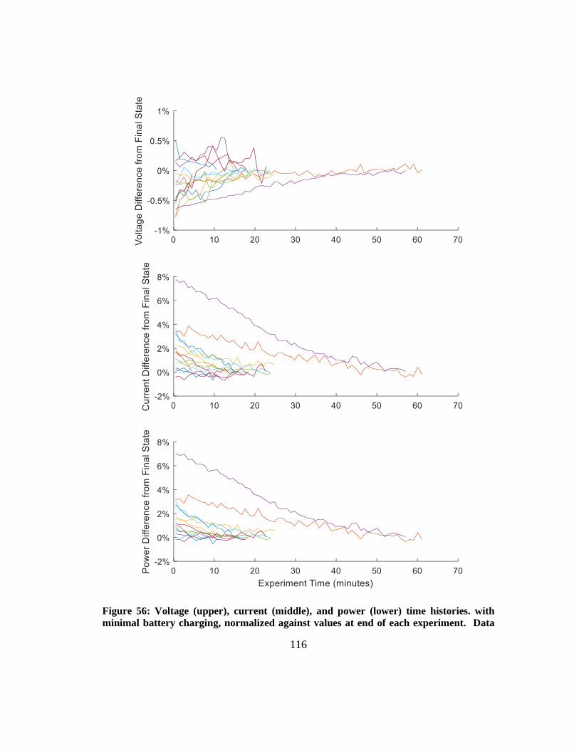
116
Figure 56: Voltage (upper), current (middle), and power (lower) time histories. with
minimal battery charging, normalized against values at end of each experiment. Data

117
represent averages over one minute and are normalized by values at end of each
experiment.
Even if the battery load is missing, we do see some change in stack power
output over time. This could be due to heating of the load bank (with higher
temperatures generating higher resistances, and so lower current demands).
Encouragingly, the variation is relatively small in most cases. However, the percent
variation from the final reading isn’t necessarily a fair representation given the
different lengths of time of each experiment—most, but not all, are approximately 20
minutes. The greatest differences, unsurprisingly, are seen in the longest experiments
with time to drift.
If we instead consider the approximate slope over time, from Figure 56 we
can tell that for even minute-to-minute data points, the slope between them can vary
drastically. If we extend the averaging time to two minutes, and evaluate the slope
between points, we can identify the point at which a threshold slope (here arbitrarily
0.1% variation per minute) is reached. These points are represented by the black dots
on each time history line in Figure 57.
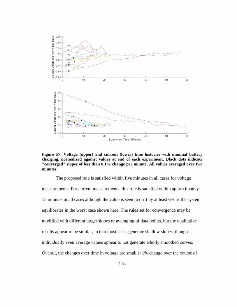
118
Figure 57: Voltage (upper) and current (lower) time histories with minimal battery
charging, normalized against values at end of each experiment. Black dots indicate
"converged" slopes of less than 0.1% change per minute. All values averaged over two
minutes.
The proposed rule is satisfied within five minutes in all cases for voltage
measurements. For current measurements, this rule is satisfied within approximately
15 minutes in all cases although the value is seen to drift by at least 6% as the system
equilibrates in the worst case shown here. The rules set for convergence may be
modified with different target slopes or averaging of data points, but the qualitative
results appear to be similar, in that most cases generate shallow slopes, though
individually even average values appear to not generate wholly smoothed curves.
Overall, the changes over time in voltage are small (<1% change over the course of
119
an experiment) compared to the changes in current output. As such, voltage values
may be acceptable as an averaged measurement over a short period of time, but
corrections may be useful for current values. “Convergence” via a slope measurement
furthermore does not reliably indicate an equilibrium value and, due to the noise in
the measurements, still requires multi-minute measurement periods which are not
ideal for the eventual use in a laboratory-scale GT-SOFC demonstrator. As such, in
the next section we will see if there might be a way to predict equilibrium
performance more quickly using nonlinear exponential decay fitting.
10.6.2 Predicting Convergence via Exponential Decay Fitting
Regression analysis using exponential functions has been used to model the
transient response of polymer electrolyte membrane (PEM) fuel cells [93] so we will
use this approach to try to predict equilibrium operating conditions without waiting
for the system to equilibrate. A least-squares nonlinear solver in MATLAB was used
to fit a function of the form 𝑓(𝑡) = 𝐴𝑒−𝑏𝑡 + 𝐶 to the data where 𝐶 is the function
value at 𝑡 = ∞ or the asymptotic value. The fitting algorithm was run over all
measurements taken for experimental trial undistorted by the battery charging (as for
Figure 56) to find the best least-squares fit values. If the fit results were outside of
reasonable ranges (negative values for either voltage or current, or values above 50
volts or 12 amps) then the initial values provided to the fitting algorithm as the
starting point of the fit were altered, and the algorithm re-run. The initial values of 𝐴,
𝑏, and 𝐶 are the same for each fitting. The value of 𝐶 can also be matched to be the

120
value of the first data point, but this yields similar results to providing the same initial
values every time, while also preventing the solver from taking the initial value for 𝐶
as ‘sufficiently converged’ already.
The results are shown in Figure 58, with the data from each experiment
plotted with its fitted curve. Most of the fits appear satisfactory (visually) although in
most cases the overall exponential decay characteristics are not strongly evident
relative to the noise level of the data. The value 𝐶 associated with each fitted curve is
assumed to be the “extrapolated” equilibrium value.
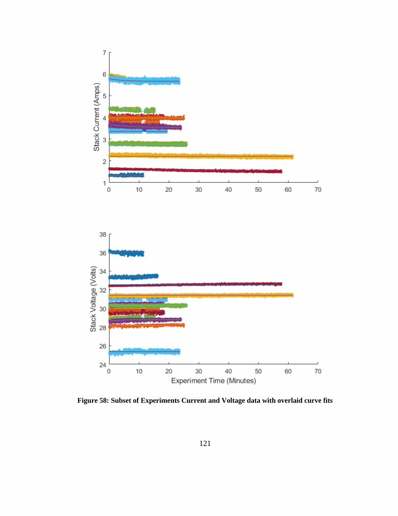
121
Figure 58: Subset of Experiments Current and Voltage data with overlaid curve fits
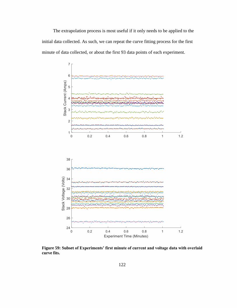
122
The extrapolation process is most useful if it only needs to be applied to the
initial data collected. As such, we can repeat the curve fitting process for the first
minute of data collected, or about the first 93 data points of each experiment.
Figure 59: Subset of Experiments’ first minute of current and voltage data with overlaid
curve fits.
123
The results again appear qualitatively linear, which is not unexpected for the
short timeframe considered. The values of 𝐶 generated by the fitting algorithm in for
all data available (~15-60 minutes depending on experiments available) tend to be
very similar! The question is whether the extrapolated equilibrium values approach
the true equilibrium conditions. Figure 60 plots normalized last-minute average
(�̅�𝑙𝑎𝑠𝑡,𝑛𝑜𝑟𝑚), 1-minute extrapolated (𝑉𝑒𝑥1,𝑛𝑜𝑟𝑚) and all-data extrapolated (𝑉𝑒𝑥𝐴𝑙𝑙,𝑛𝑜𝑟𝑚)
voltage and equivalent current values, all normalized (as shown in Equation (29)) by
the average value of the first minute of data collected (�̅�𝑓𝑖𝑟𝑠𝑡) since all data collection
regimes will have this data available.
�̅�𝑙𝑎𝑠𝑡,𝑛𝑜𝑟𝑚 = �̅�𝑙𝑎𝑠𝑡/�̅�𝑓𝑖𝑟𝑠𝑡 (29)
Lines are drawn to connect the last-minute values and their associated
extrapolations from the same experiment to show drift between the methods.
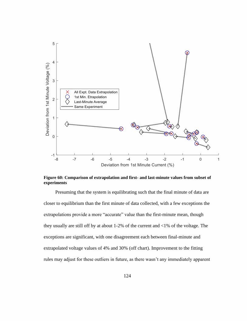
124
Figure 60: Comparison of extrapolation and first- and last-minute values from subset of
experiments
Presuming that the system is equilibrating such that the final minute of data are
closer to equilibrium than the first minute of data collected, with a few exceptions the
extrapolations provide a more “accurate” value than the first-minute mean, though
they usually are still off by at about 1-2% of the current and <1% of the voltage. The
exceptions are significant, with one disagreement each between final-minute and
extrapolated voltage values of 4% and 30% (off chart). Improvement to the fitting
rules may adjust for these outliers in future, as there wasn’t any immediately apparent
125
explanation for the discrepancy. There is also no immediately discernible trend of the
extrapolations overshooting or undershooting the last-minute value.
In both the cases of establishing convergence to the equilibrium and of
predicting convergence values, the data are obscured by the varying loads and
adjustments of the balance of plant, control system, and load bank. Future work will
involve disconnecting the SOFC stack from the balance of plant, and improvements
to the load bank for constant-current and automated data collection may improve the
quality of the data collected such that the processes outlined in this section may yield
more reliable results. As of this time however, practically speaking simply averaging
the initial measurements will still fall within ranges of ±2% for voltage values and
worst case ±10% for current value, as compared to measurements taken at long times
(≥20 minutes) thereafter. Extrapolations using first-minute data will generally
provide an improvement towards equilibrium, but not yet reliably with the current
fitting method.
Overall, the results presented previously in Figure 55 capture the performance
of the AMI APU over a variety of loads and may be sufficient for developing a
preliminary model of the bench-scale GT/SOFC hybrid. However, all of the
experiments have been conducted at atmospheric pressure whereas pressures in the
gas turbine’s combustor are ~ 3 atm. While there are crude methods for extrapolating
these results to higher pressures (such as tuning the model to match results at the
lower operating condition), more measurements at elevated pressures are required.
Also of interest would be finding ways to infer equilibrium voltage and current from

126
time histories that are not converged and measuring more detailed aspects of the fuel
cell’s performance like ohmic, activation, and concentration losses. Measuring the
latter may be easier when the system is disassembled but is not possible now while
the APU control system is activated, and could entail analysis using electronic
impedance spectroscopy if available to generate equivalent polarization curves for
comparison of results.

127
11 Preliminary Design of a Bench-Scale GT/SOFC Hybrid
Finally we will consider an initial NPSS model of a laboratory-scale GT-
SOFC hybrid based on the small turbojet engine described in section 6.3.3 and the
APU described in Chapter 10. The results provide insight into how to design the
prototype by indicating what conditions (i.e. pressure, temperature, flow rate) will
need to be accommodated where. This section is based closely upon a previous
conference paper by the author.[4]
11.1 GT Model
The full characterization and NPSS model validation for the AMT Olympus
High Power system has been addressed in prior work by Vannoy and Cadou [61],
with substantial refinements by Vannoy [62] that were not available in time to be
included in the integrated analysis. The NPSS model components and system settings
produced were used as the basis for conversion into a GT-SOFC, with design
parameters provided below in Table 7.
Table 7: Baseline conditions for NPSS model of AMT Olympus HP, adapted from [61]
Parameter Value
RPM 108,500
Air Flowrate (lbm/sec) 0.99
Compressor Total Pressure Ratio (𝑷𝟎𝟑/𝑷𝟎𝟐) 3.7
Compressor Efficiency 0.75
Fuel Type Jet-A
Fuel Flowrate (lbm/sec) 0.0262
Turbine Total Pressure Ratio (𝑷𝟎𝟒/𝑷𝟎𝟓) 2.148
Turbine Efficiency 0.729
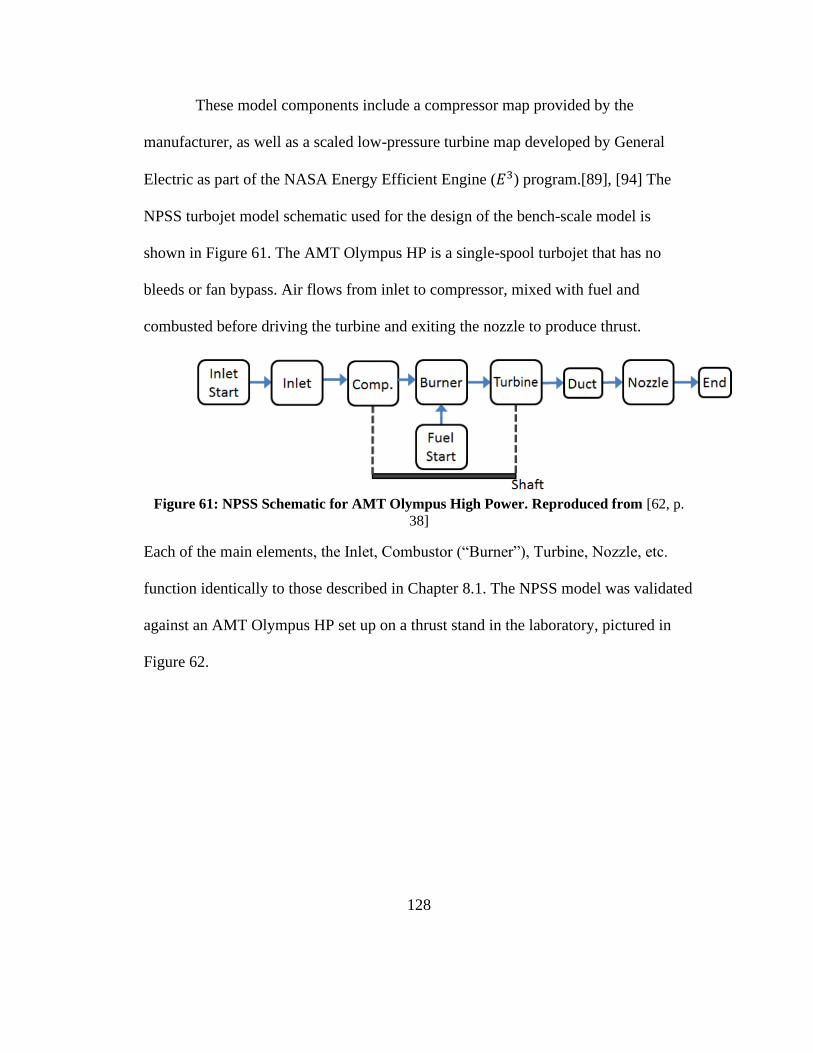
128
These model components include a compressor map provided by the
manufacturer, as well as a scaled low-pressure turbine map developed by General
Electric as part of the NASA Energy Efficient Engine (𝐸3) program.[89], [94] The
NPSS turbojet model schematic used for the design of the bench-scale model is
shown in Figure 61. The AMT Olympus HP is a single-spool turbojet that has no
bleeds or fan bypass. Air flows from inlet to compressor, mixed with fuel and
combusted before driving the turbine and exiting the nozzle to produce thrust.
Figure 61: NPSS Schematic for AMT Olympus High Power. Reproduced from [62, p.
38]
Each of the main elements, the Inlet, Combustor (“Burner”), Turbine, Nozzle, etc.
function identically to those described in Chapter 8.1. The NPSS model was validated
against an AMT Olympus HP set up on a thrust stand in the laboratory, pictured in
Figure 62.
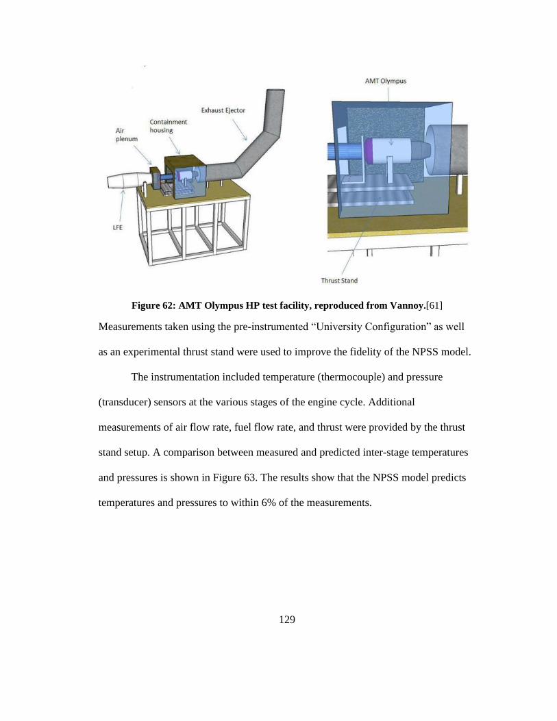
129
Figure 62: AMT Olympus HP test facility, reproduced from Vannoy.[61]
Measurements taken using the pre-instrumented “University Configuration” as well
as an experimental thrust stand were used to improve the fidelity of the NPSS model.
The instrumentation included temperature (thermocouple) and pressure
(transducer) sensors at the various stages of the engine cycle. Additional
measurements of air flow rate, fuel flow rate, and thrust were provided by the thrust
stand setup. A comparison between measured and predicted inter-stage temperatures
and pressures is shown in Figure 63. The results show that the NPSS model predicts
temperatures and pressures to within 6% of the measurements.
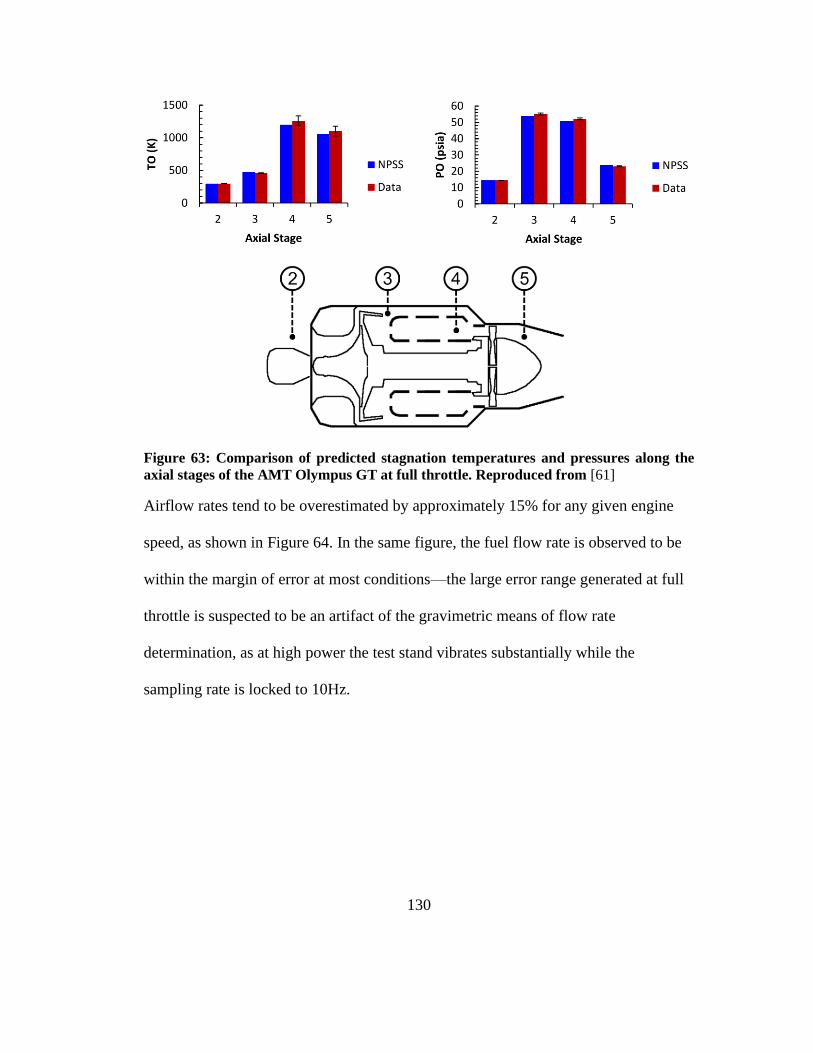
130
Figure 63: Comparison of predicted stagnation temperatures and pressures along the
axial stages of the AMT Olympus GT at full throttle. Reproduced from [61]
Airflow rates tend to be overestimated by approximately 15% for any given engine
speed, as shown in Figure 64. In the same figure, the fuel flow rate is observed to be
within the margin of error at most conditions—the large error range generated at full
throttle is suspected to be an artifact of the gravimetric means of flow rate
determination, as at high power the test stand vibrates substantially while the
sampling rate is locked to 10Hz.
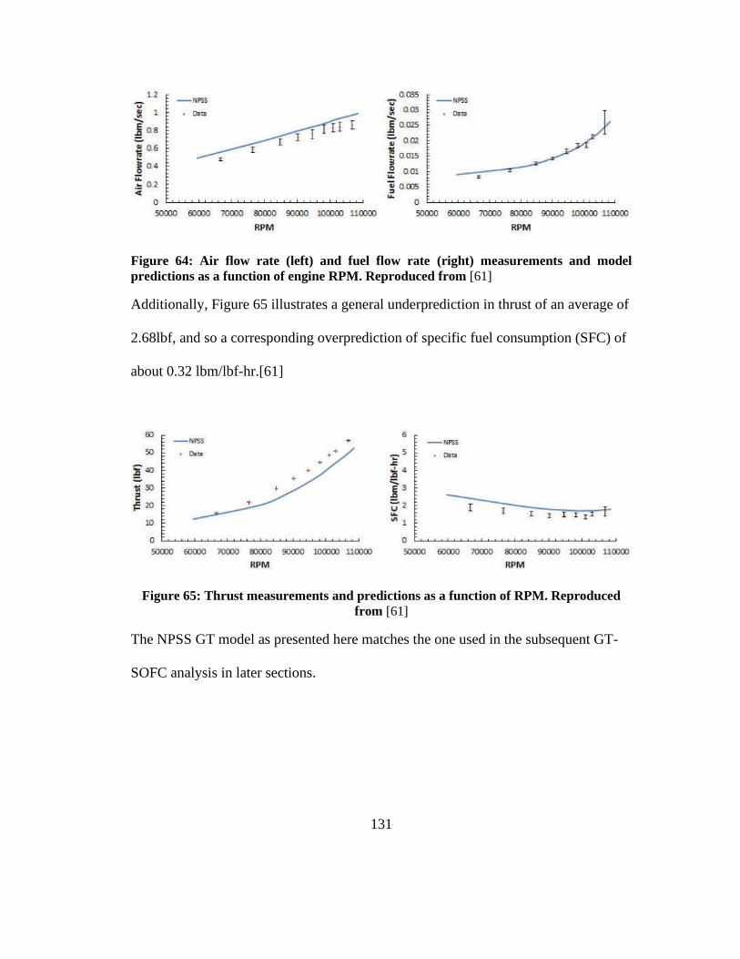
131
Figure 64: Air flow rate (left) and fuel flow rate (right) measurements and model
predictions as a function of engine RPM. Reproduced from [61]
Additionally, Figure 65 illustrates a general underprediction in thrust of an average of
2.68lbf, and so a corresponding overprediction of specific fuel consumption (SFC) of
about 0.32 lbm/lbf-hr.[61]
Figure 65: Thrust measurements and predictions as a function of RPM. Reproduced
from [61]
The NPSS GT model as presented here matches the one used in the subsequent GT-
SOFC analysis in later sections.
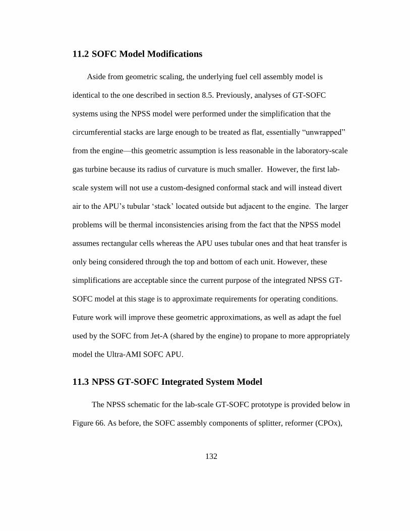
132
11.2 SOFC Model Modifications
Aside from geometric scaling, the underlying fuel cell assembly model is
identical to the one described in section 8.5. Previously, analyses of GT-SOFC
systems using the NPSS model were performed under the simplification that the
circumferential stacks are large enough to be treated as flat, essentially “unwrapped”
from the engine—this geometric assumption is less reasonable in the laboratory-scale
gas turbine because its radius of curvature is much smaller. However, the first lab-
scale system will not use a custom-designed conformal stack and will instead divert
air to the APU’s tubular ‘stack’ located outside but adjacent to the engine. The larger
problems will be thermal inconsistencies arising from the fact that the NPSS model
assumes rectangular cells whereas the APU uses tubular ones and that heat transfer is
only being considered through the top and bottom of each unit. However, these
simplifications are acceptable since the current purpose of the integrated NPSS GT-
SOFC model at this stage is to approximate requirements for operating conditions.
Future work will improve these geometric approximations, as well as adapt the fuel
used by the SOFC from Jet-A (shared by the engine) to propane to more appropriately
model the Ultra-AMI SOFC APU.
11.3 NPSS GT-SOFC Integrated System Model
The NPSS schematic for the lab-scale GT-SOFC prototype is provided below in
Figure 66. As before, the SOFC assembly components of splitter, reformer (CPOx),
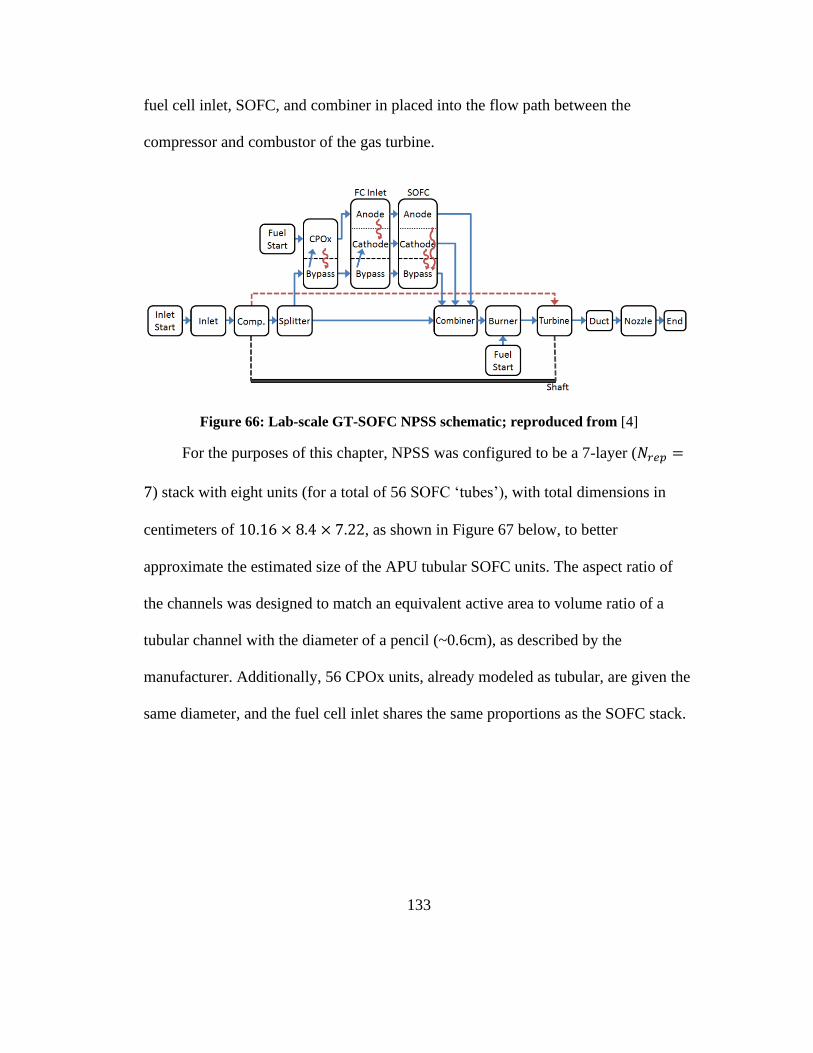
133
fuel cell inlet, SOFC, and combiner in placed into the flow path between the
compressor and combustor of the gas turbine.
Figure 66: Lab-scale GT-SOFC NPSS schematic; reproduced from [4]
For the purposes of this chapter, NPSS was configured to be a 7-layer (𝑁𝑟𝑒𝑝 =
7) stack with eight units (for a total of 56 SOFC ‘tubes’), with total dimensions in
centimeters of 10.16 × 8.4 × 7.22, as shown in Figure 67 below, to better
approximate the estimated size of the APU tubular SOFC units. The aspect ratio of
the channels was designed to match an equivalent active area to volume ratio of a
tubular channel with the diameter of a pencil (~0.6cm), as described by the
manufacturer. Additionally, 56 CPOx units, already modeled as tubular, are given the
same diameter, and the fuel cell inlet shares the same proportions as the SOFC stack.
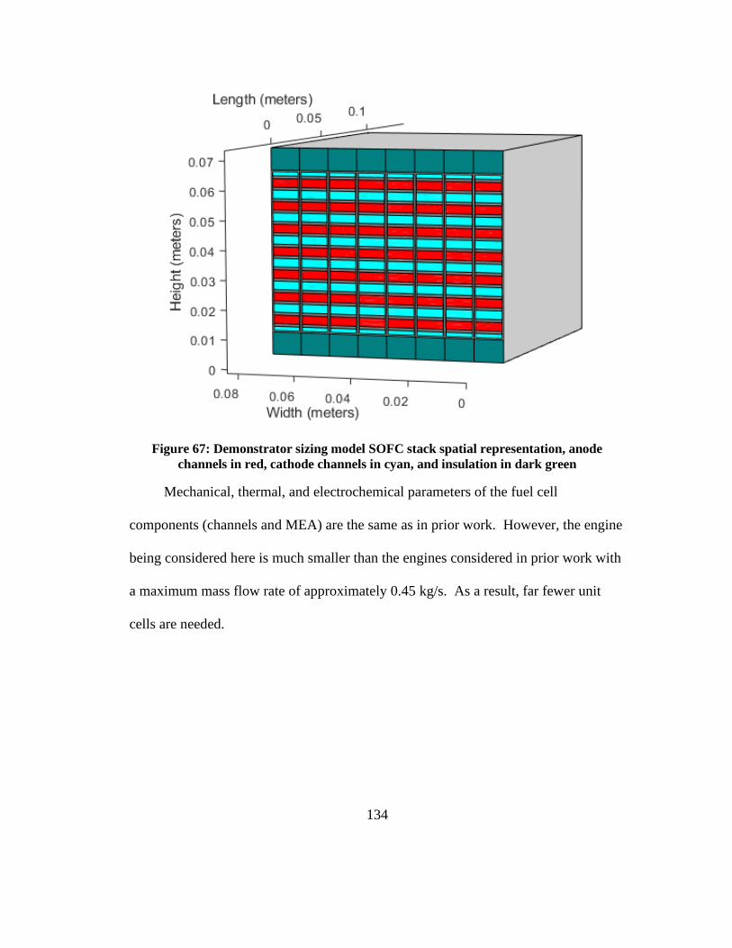
134
Figure 67: Demonstrator sizing model SOFC stack spatial representation, anode
channels in red, cathode channels in cyan, and insulation in dark green
Mechanical, thermal, and electrochemical parameters of the fuel cell
components (channels and MEA) are the same as in prior work. However, the engine
being considered here is much smaller than the engines considered in prior work with
a maximum mass flow rate of approximately 0.45 kg/s. As a result, far fewer unit
cells are needed.

135
11.4 Results
11.4.1 Model Validation
While the electrochemical model used in this work has been previously
validated,[80] a limited validation of the GT-SOFC model was performed by solving
the model for a range of stack voltage conditions to generate a polarization curve for
the integrated system while at full throttle at sea-level-static (SLS, i.e. laboratory)
conditions, shown in Figure 68. The intent is to show that “reasonable” results are
produced, rather than attempt to model a specific SOFC system at this point in
development.
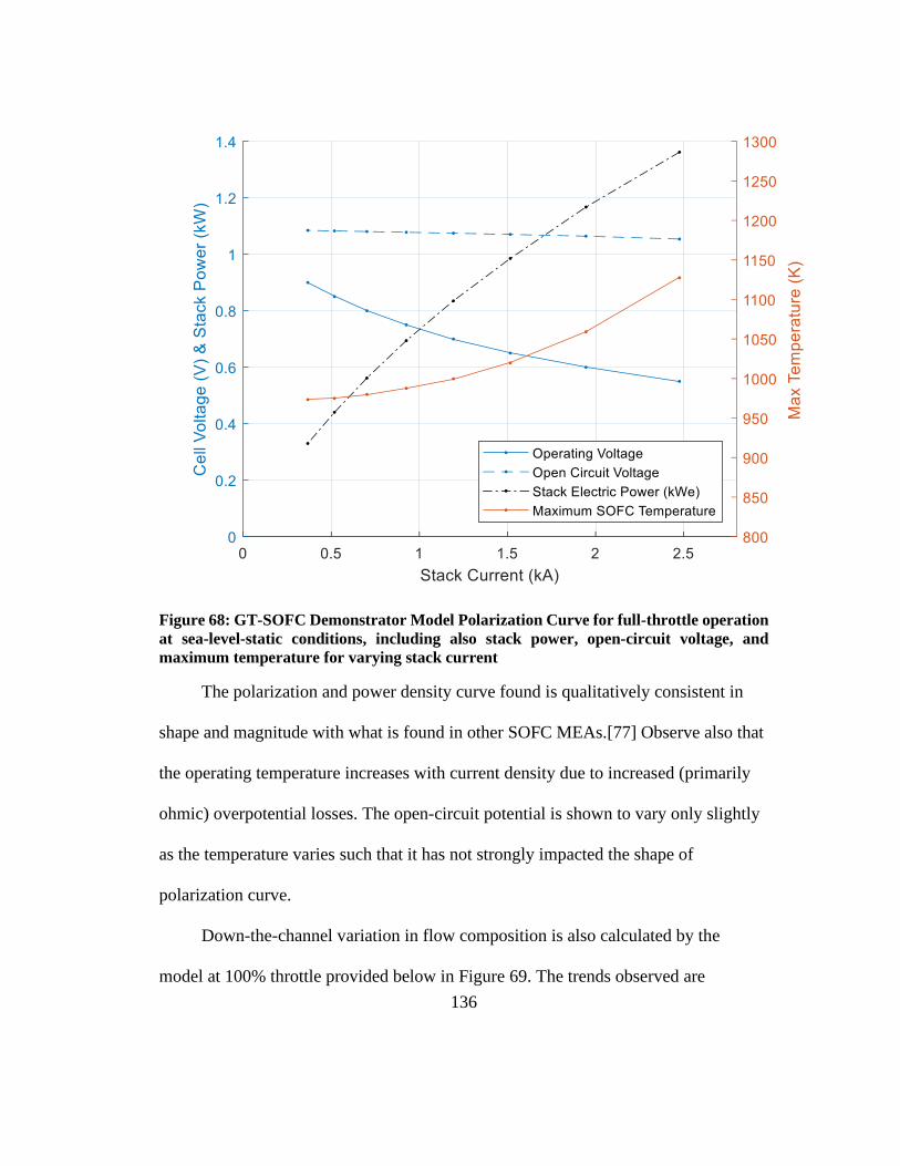
136
Figure 68: GT-SOFC Demonstrator Model Polarization Curve for full-throttle operation
at sea-level-static conditions, including also stack power, open-circuit voltage, and
maximum temperature for varying stack current
The polarization and power density curve found is qualitatively consistent in
shape and magnitude with what is found in other SOFC MEAs.[77] Observe also that
the operating temperature increases with current density due to increased (primarily
ohmic) overpotential losses. The open-circuit potential is shown to vary only slightly
as the temperature varies such that it has not strongly impacted the shape of
polarization curve.
Down-the-channel variation in flow composition is also calculated by the
model at 100% throttle provided below in Figure 69. The trends observed are
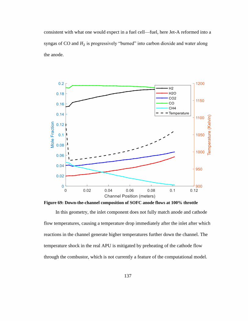
137
consistent with what one would expect in a fuel cell—fuel, here Jet-A reformed into a
syngas of CO and 𝐻2 is progressively “burned” into carbon dioxide and water along
the anode.
Figure 69: Down-the-channel composition of SOFC anode flows at 100% throttle
In this geometry, the inlet component does not fully match anode and cathode
flow temperatures, causing a temperature drop immediately after the inlet after which
reactions in the channel generate higher temperatures further down the channel. The
temperature shock in the real APU is mitigated by preheating of the cathode flow
through the combustor, which is not currently a feature of the computational model.
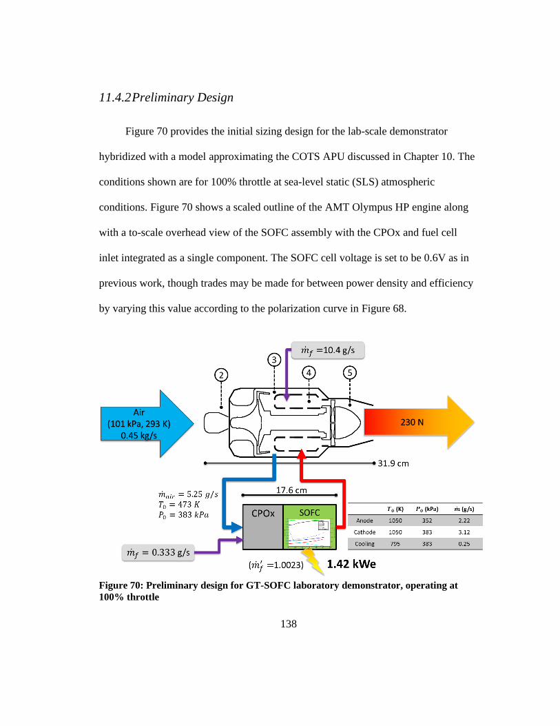
138
11.4.2 Preliminary Design
Figure 70 provides the initial sizing design for the lab-scale demonstrator
hybridized with a model approximating the COTS APU discussed in Chapter 10. The
conditions shown are for 100% throttle at sea-level static (SLS) atmospheric
conditions. Figure 70 shows a scaled outline of the AMT Olympus HP engine along
with a to-scale overhead view of the SOFC assembly with the CPOx and fuel cell
inlet integrated as a single component. The SOFC cell voltage is set to be 0.6V as in
previous work, though trades may be made for between power density and efficiency
by varying this value according to the polarization curve in Figure 68.
Figure 70: Preliminary design for GT-SOFC laboratory demonstrator, operating at
100% throttle

139
There are several conclusions that may be drawn from the design as provided.
First is that the power output is more than four times greater than the real-life APU
(1.42kWe vs. 300We). This is likely due to the higher pressure conditions inside the
cell (~3.8 atm) and a greater fuel flow rate, as well as the lack of balance-of-plant
demands and other non-idealities.
Second, the fuel cell assembly requires a relatively small proportion of air from
the gas turbine, slightly over 1%. Additionally, the overall relative fuel flow rate
(1.0023) is less than 1% more than the gas turbine alone for the same performance.
This value is nearly identical to that a mechanical generator producing the same
amount of electric power, but this is almost certainly due to the relatively low amount
electric power requirement—however the usual metric of electric power fraction is
additionally difficult to ascertain for SLS conditions since the gas turbine is
producing zero power while held in place on a thrust stand.
Finally, we may note that there are three different exhaust streams from the fuel
cell assembly with anode and cathode temperatures only 50K short of the combustor
exhaust temperature of 1100K and essentially no substantial pressure losses for the
cathode and cooling air channels. A current problem to be resolved is the lowered
pressure of the anode flow (which underwent combustion) which will require
pressure matching of some kind in order to integrate with the higher-pressure gas
turbine combustor.
140
12 Conclusions and Future Work
12.1 Conclusions
12.1.1 Summary
Over the course of this thesis, several related projects were pursued surrounding
the concept of GT-SOFC hybrid systems for aircraft. Building off of prior work to
develop the integrated GT-SOFC model, we have investigated the effects of drag –
both induced (due to the extra mass of the components) and profile (due to the
protrusion of fuel cell components into the air flow in pylon-mounted configurations)
on the efficacy of GT-SOFC hybrids in regional transport jets and high-altitude, long-
endurance aircraft like the RQ-4 Global Hawk. The results have demonstrated the
greater impact and sensitivity of the outfitted aircraft to profile drag rather than drag
penalty represented by the additional mass alone. This conclusion allows us to
prioritize design decisions to minimize profile drag. Furthermore, a more-detailed
sensitivity analysis has been performed or revised for several system characteristics.
However, the exploration of drag was still wholly theoretical, and performed
entirely within NPSS. Looking to the need to validate our modeling efforts against a
real-world system, we collected and characterized COTS components to serve as the
basis of a demonstrator system. The COTS APU was characterized as part of this
work by measuring the stack’s polarization curve. In the process, methods of
operating the fuel cell and analyzing the available output for effective data collection

141
were explored, yielding an initial polarization curve and providing guidance to speed
up future data collection activities.
Looking ahead to the integration of the COTS GT and SOFC APU systems in a
bench-scale system, a model of such a system was created in NPSS in order to guide
the development of hardware when it is finally time to “bend metal” to create the
prototype GT-SOFC.
12.1.2 Author Contributions
In pursuing the research discussed in this thesis, the author made several personal
contributions to the project. These have included improvements to the modeling of
external aerodynamic drag (both induced and profile drag) and investigations into the
role these penalties play in limiting the performance advantage of integrated GT-
SOFCs in aircraft (Chapter 9). Additionally, the author has expanded and corrected
the associated sensitivity analyses necessary to confirm the ability of the model to
generate meaningful results. Through these efforts, the author has helped to identify
aerodynamic drag as a key performance limiter for GT-SOFC systems in aircraft.
Looking towards the development of a laboratory-scale GT-SOFC
demonstrator, the author was responsible for the design, construction, and operation
of an experimental apparatus to measure the performance of an off-the-shelf SOFC
APU that will later serve as the basis of the SOFC assembly in the demonstrator
system. This process included both hardware and software design to devise a load
bank and data collection method and routine, using a hobbyist Linux computer and

142
scripting to take the place of LabView for a non-standard interface. The author has
collected many hours of data produced by the apparatus and successfully processed
them into the results presented in Chapter 10, characterizing an SOFC APU. As part
of this analysis, the author has devised more rapid procedures for measuring SOFC
APU performance without having to wait for full equilibration, which will enable
data collection from an integrated GT-SOFC on a reasonable timescale.
The SOFC APU was also approached from the direction of simulation, as the
author has developed an NPSS model of the SOFC APU and integrated the model
with an NPSS model of a COTS turbojet engine, using the resulting integrated model
to create an initial design for the lab-scale demonstrator system (Chapter 11). The
author also analyzed the integrated model for its relative performance against a
traditional turbojet outfitted with a mechanical generator for electricity production.
Finally, the author undertook several projects to improve the NPSS GT-SOFC
model code base, including the transfer of the project to rigorous version control and
project tracking, enabling easy access/distribution to sponsors and collaborators. The
author has also developed tools to minimize the impact of the currently slow (often
weeks of runtime) calculation speed. In particular, the author has replaced custom
viewer files in favor of a dump of all variables to disk, building on that standard
capability with scripts to sort and tabulate the results for easy processing in analysis
software such as MATLAB. Additionally, this method retains the option to retrieve
any new variable used by the calculation immediately without having to re-run the
entire simulation just for adding an entry to the Viewer file. Also, convenience
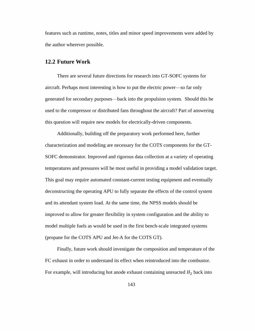
143
features such as runtime, notes, titles and minor speed improvements were added by
the author wherever possible.
12.2 Future Work
There are several future directions for research into GT-SOFC systems for
aircraft. Perhaps most interesting is how to put the electric power—so far only
generated for secondary purposes—back into the propulsion system. Should this be
used to the compressor or distributed fans throughout the aircraft? Part of answering
this question will require new models for electrically-driven components.
Additionally, building off the preparatory work performed here, further
characterization and modeling are necessary for the COTS components for the GT-
SOFC demonstrator. Improved and rigorous data collection at a variety of operating
temperatures and pressures will be most useful in providing a model validation target.
This goal may require automated constant-current testing equipment and eventually
deconstructing the operating APU to fully separate the effects of the control system
and its attendant system load. At the same time, the NPSS models should be
improved to allow for greater flexibility in system configuration and the ability to
model multiple fuels as would be used in the first bench-scale integrated systems
(propane for the COTS APU and Jet-A for the COTS GT).
Finally, future work should investigate the composition and temperature of the
FC exhaust in order to understand its effect when reintroduced into the combustor.
For example, will introducing hot anode exhaust containing unreacted 𝐻2 back into

144
the combustor lead to potentially damaging hot spots? Or alternately could the
exhaust be used to reduce thermal 𝑁𝑂𝑥 formation by enhancing flame stability,
enabling operation at lower overall equivalence ratios.
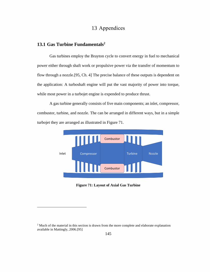
145
13 Appendices
13.1 Gas Turbine Fundamentals2
Gas turbines employ the Brayton cycle to convert energy in fuel to mechanical
power either through shaft work or propulsive power via the transfer of momentum to
flow through a nozzle.[95, Ch. 4] The precise balance of these outputs is dependent on
the application: A turboshaft engine will put the vast majority of power into torque,
while most power in a turbojet engine is expended to produce thrust.
A gas turbine generally consists of five main components; an inlet, compressor,
combustor, turbine, and nozzle. The can be arranged in different ways, but in a simple
turbojet they are arranged as illustrated in Figure 71.
Figure 71: Layout of Axial Gas Turbine
2 Much of the material in this section is drawn from the more complete and elaborate explanation
available in Mattingly, 2006.[95]
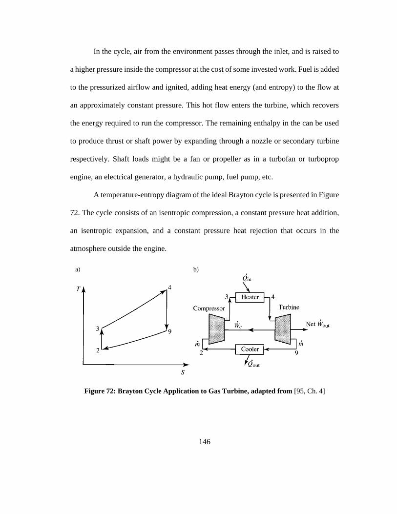
146
In the cycle, air from the environment passes through the inlet, and is raised to
a higher pressure inside the compressor at the cost of some invested work. Fuel is added
to the pressurized airflow and ignited, adding heat energy (and entropy) to the flow at
an approximately constant pressure. This hot flow enters the turbine, which recovers
the energy required to run the compressor. The remaining enthalpy in the can be used
to produce thrust or shaft power by expanding through a nozzle or secondary turbine
respectively. Shaft loads might be a fan or propeller as in a turbofan or turboprop
engine, an electrical generator, a hydraulic pump, fuel pump, etc.
A temperature-entropy diagram of the ideal Brayton cycle is presented in Figure
72. The cycle consists of an isentropic compression, a constant pressure heat addition,
an isentropic expansion, and a constant pressure heat rejection that occurs in the
atmosphere outside the engine.
Figure 72: Brayton Cycle Application to Gas Turbine, adapted from [95, Ch. 4]

147
Practically speaking, the limits on the performance of the gas turbine are the
maximum material temperature limit of the combustor and turbine inlet, as well as the
compression ratio which is limited by the size and efficiency of compressor
components. More important for this work are the effects that variations in pressure
and temperature of operation have on the fuel cell portions of the overall system.

148
13.2 Fuel Cell Fundamentals3
Like engines, fuel cells produce electrical power by reacting hydrogen-bearing
fuel with oxidizer to produce water and additional products like carbon dioxide. Unlike
engines, most of the energy release drives electrons through a potential gradient
producing electrical power directly, as opposed to heating a working fluid that does
work through expansion. In the fuel cell, reactants flow in two streams (fuel and
oxidizer) through adjacent channels separated by walls called the membrane-electrode
assembly (MEA). The MEA is made up of three main layers. The outer two layers in
contact with the reactants are called electrodes and permit the transport of both ions
and electrical charge.
The difference in chemical potential between reactions occurring on the
electrodes drives the flow of electrons in the system. The nature of the reaction that
occurs on each electrode depends on which reactant flow it contacts, with the fuel
stream undergoing oxidation reactions (with the electrode designated the “anode”) and
the oxidizer stream undergoing reduction reactions (with the electrode designated the
“cathode”). Reactions occurring on the surfaces of the electrodes are usually enabled
and accelerated by a catalyst coating that improves the rate of power conversion on a
given surface area.
3 Much of the material in this section is drawn from the more elaborate explanations available in
Principles of Fuel Cells by Xianguo Li.[10]
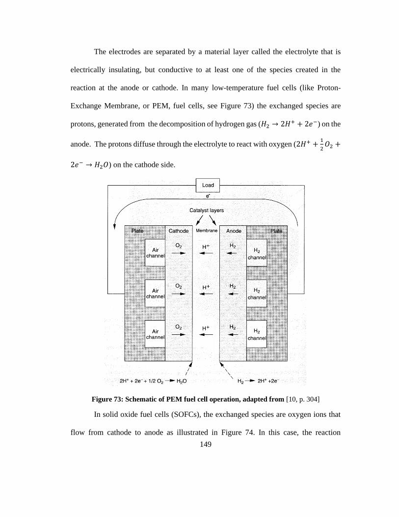
149
The electrodes are separated by a material layer called the electrolyte that is
electrically insulating, but conductive to at least one of the species created in the
reaction at the anode or cathode. In many low-temperature fuel cells (like Proton-
Exchange Membrane, or PEM, fuel cells, see Figure 73) the exchanged species are
protons, generated from the decomposition of hydrogen gas (𝐻2 → 2𝐻+ + 2𝑒−) on the
anode. The protons diffuse through the electrolyte to react with oxygen (2𝐻+ +1
2𝑂2 +
2𝑒− → 𝐻2𝑂) on the cathode side.
Figure 73: Schematic of PEM fuel cell operation, adapted from [10, p. 304]
In solid oxide fuel cells (SOFCs), the exchanged species are oxygen ions that
flow from cathode to anode as illustrated in Figure 74. In this case, the reaction
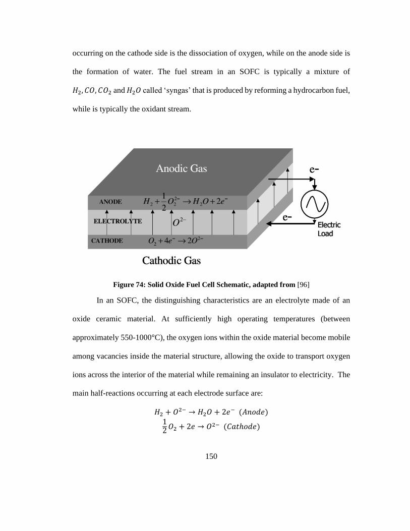
150
occurring on the cathode side is the dissociation of oxygen, while on the anode side is
the formation of water. The fuel stream in an SOFC is typically a mixture of
𝐻2, 𝐶𝑂, 𝐶𝑂2 and 𝐻2𝑂 called ‘syngas’ that is produced by reforming a hydrocarbon fuel,
while is typically the oxidant stream.
Figure 74: Solid Oxide Fuel Cell Schematic, adapted from [96]
In an SOFC, the distinguishing characteristics are an electrolyte made of an
oxide ceramic material. At sufficiently high operating temperatures (between
approximately 550-1000°C), the oxygen ions within the oxide material become mobile
among vacancies inside the material structure, allowing the oxide to transport oxygen
ions across the interior of the material while remaining an insulator to electricity. The
main half-reactions occurring at each electrode surface are:
𝐻2 + 𝑂2− → 𝐻2𝑂 + 2𝑒
− (𝐴𝑛𝑜𝑑𝑒)12𝑂2 + 2𝑒 → 𝑂
2− (𝐶𝑎𝑡ℎ𝑜𝑑𝑒)
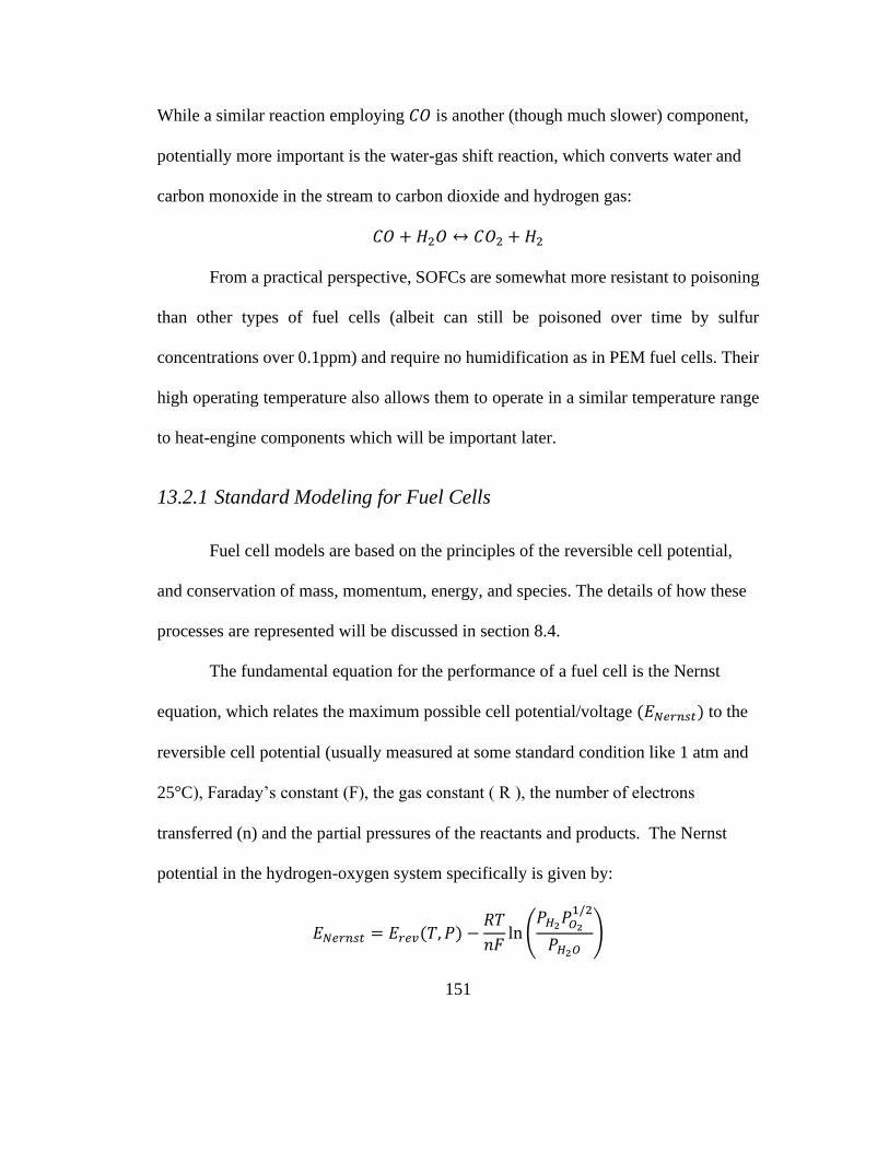
151
While a similar reaction employing 𝐶𝑂 is another (though much slower) component,
potentially more important is the water-gas shift reaction, which converts water and
carbon monoxide in the stream to carbon dioxide and hydrogen gas:
𝐶𝑂 + 𝐻2𝑂 ↔ 𝐶𝑂2 + 𝐻2
From a practical perspective, SOFCs are somewhat more resistant to poisoning
than other types of fuel cells (albeit can still be poisoned over time by sulfur
concentrations over 0.1ppm) and require no humidification as in PEM fuel cells. Their
high operating temperature also allows them to operate in a similar temperature range
to heat-engine components which will be important later.
13.2.1 Standard Modeling for Fuel Cells
Fuel cell models are based on the principles of the reversible cell potential,
and conservation of mass, momentum, energy, and species. The details of how these
processes are represented will be discussed in section 8.4.
The fundamental equation for the performance of a fuel cell is the Nernst
equation, which relates the maximum possible cell potential/voltage (𝐸𝑁𝑒𝑟𝑛𝑠𝑡) to the
reversible cell potential (usually measured at some standard condition like 1 atm and
25°C), Faraday’s constant (F), the gas constant ( R ), the number of electrons
transferred (n) and the partial pressures of the reactants and products. The Nernst
potential in the hydrogen-oxygen system specifically is given by:
𝐸𝑁𝑒𝑟𝑛𝑠𝑡 = 𝐸𝑟𝑒𝑣(𝑇, 𝑃) −𝑅𝑇
𝑛𝐹ln(
𝑃𝐻2𝑃𝑂21/2
𝑃𝐻2𝑂)

152
For the hydrogen-oxygen system 𝑛 = 2. The Nernst potential is the maximum
potential that is thermodynamically achievable, but the potential of a real cell is lower
because of various loss processes. These losses are represented using ‘overpotentials’
(𝜂) so that the expression for the actual cell voltage can be given by:
𝐸𝑐𝑒𝑙𝑙 = 𝐸𝑁𝑒𝑟𝑛𝑠𝑡 − 𝜂𝑎𝑐𝑡 − 𝜂𝑜ℎ𝑚 − 𝜂𝑐𝑜𝑛𝑐
Activation overpotentials (𝜂𝑎𝑐𝑡) are related to the excess energy needed to
cause a reaction to occur spontaneously (the “activation energy”) by overcoming any
energetically unfavorable conditions in the transition between reactants and products.
Ohmic overpotentials (𝜂𝑜ℎ𝑚) are associated with resistive losses throughout the
system, both at electrodes and through system wiring. Finally, concentration
overpotentials (𝜂𝑐𝑜𝑛𝑐) are related to the kinetics of the system at the electrodes, such
that gradients of products and reactants can be expected to form, affecting the
effective concentration at the location where reactions occur.
For SOFCs, the activation and concentration overpotentials are often small
due to the high operating temperature and electrode catalysts, which create fast
reaction kinetics and rapid mass diffusion. However, the corresponding ohmic losses
are significant, generating almost linear losses to voltage with increasing current.
Taken together, these losses can be used to generate a polarization curve which is a
standard way of representing fuel cell performance.
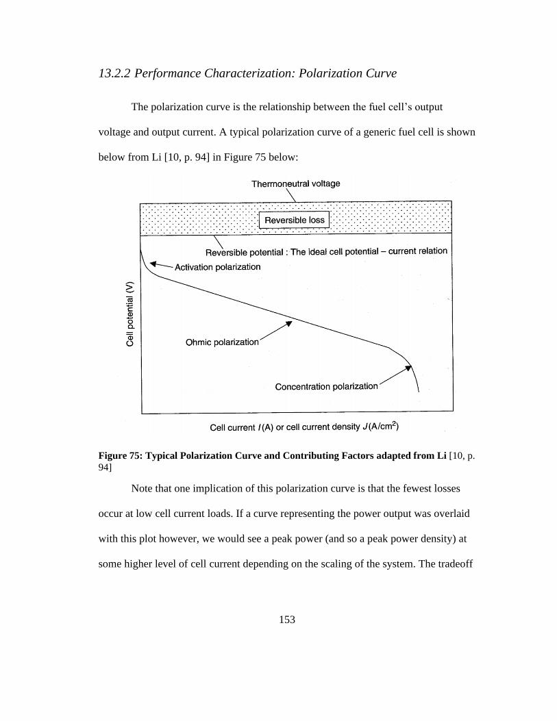
153
13.2.2 Performance Characterization: Polarization Curve
The polarization curve is the relationship between the fuel cell’s output
voltage and output current. A typical polarization curve of a generic fuel cell is shown
below from Li [10, p. 94] in Figure 75 below:
Figure 75: Typical Polarization Curve and Contributing Factors adapted from Li [10, p.
94]
Note that one implication of this polarization curve is that the fewest losses
occur at low cell current loads. If a curve representing the power output was overlaid
with this plot however, we would see a peak power (and so a peak power density) at
some higher level of cell current depending on the scaling of the system. The tradeoff
154
between efficiency and power density is important for mass-sensitive applications
such as aircraft.
13.2.3 Efficiency Paradigm
The limits of efficiency of a fuel cell are fundamentally the same as those of a
heat engine than a heat engine cycle, with both based on the second law of
thermodynamics (yielding so-called “second law efficiencies”). [10, p. 83] The
equation for the maximum efficiency of a reversible process (applying to both ideal
fuel cells and ideal heat engines) is the ratio of Gibbs Free Energy (Δ𝑔) to Enthalpy
(Δℎ) available. The Gibbs energy is also the negative of the work out (𝑤) in the
reversible case:
𝜂𝑟𝑒𝑣 =Δ𝑔(𝑇, 𝑃)
Δℎ(𝑇, 𝑃)=−𝑤
Δℎ
In the special case of a heat engine, the system operates between at least two thermal
energy reservoirs (TERs), one at a high (𝑇𝐻) and one at a low (𝑇𝐿) temperature state.
Heat energy is drawn from the hot TER (𝑞𝐿) and absorbed by the cool TER (𝑞𝐿). For
the ideal reversible case, according to the first law of thermodynamics the difference
in the two heat quantities represents the amount of work (𝑤) generated by the heat
engine:
𝑤 = 𝑞𝐻 − 𝑞𝐿
The second law of thermodynamics for a reversible system (the case for the maximum
efficiency) implies that 𝑞 = 𝑇Δ𝑠 at both TERs, such that:
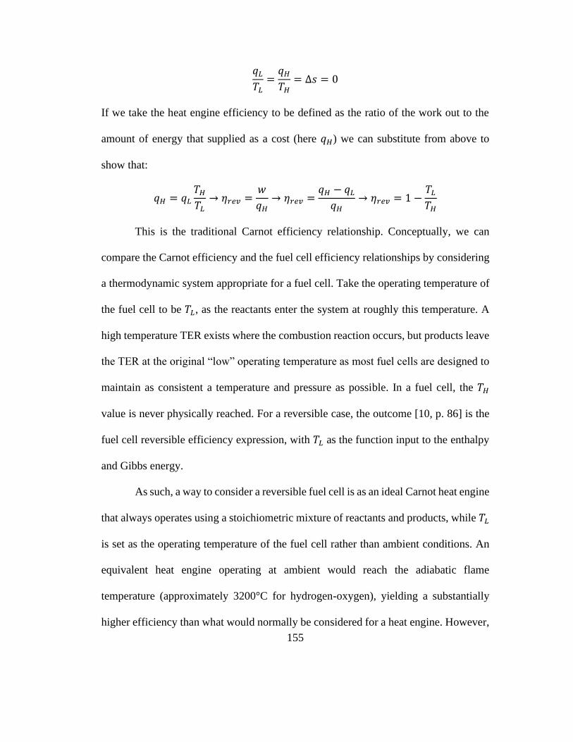
155
𝑞𝐿𝑇𝐿=𝑞𝐻𝑇𝐻= Δ𝑠 = 0
If we take the heat engine efficiency to be defined as the ratio of the work out to the
amount of energy that supplied as a cost (here 𝑞𝐻) we can substitute from above to
show that:
𝑞𝐻 = 𝑞𝐿𝑇𝐻𝑇𝐿→ 𝜂𝑟𝑒𝑣 =
𝑤
𝑞𝐻→ 𝜂𝑟𝑒𝑣 =
𝑞𝐻 − 𝑞𝐿𝑞𝐻
→ 𝜂𝑟𝑒𝑣 = 1 −𝑇𝐿𝑇𝐻
This is the traditional Carnot efficiency relationship. Conceptually, we can
compare the Carnot efficiency and the fuel cell efficiency relationships by considering
a thermodynamic system appropriate for a fuel cell. Take the operating temperature of
the fuel cell to be 𝑇𝐿, as the reactants enter the system at roughly this temperature. A
high temperature TER exists where the combustion reaction occurs, but products leave
the TER at the original “low” operating temperature as most fuel cells are designed to
maintain as consistent a temperature and pressure as possible. In a fuel cell, the 𝑇𝐻
value is never physically reached. For a reversible case, the outcome [10, p. 86] is the
fuel cell reversible efficiency expression, with 𝑇𝐿 as the function input to the enthalpy
and Gibbs energy.
As such, a way to consider a reversible fuel cell is as an ideal Carnot heat engine
that always operates using a stoichiometric mixture of reactants and products, while 𝑇𝐿
is set as the operating temperature of the fuel cell rather than ambient conditions. An
equivalent heat engine operating at ambient would reach the adiabatic flame
temperature (approximately 3200°C for hydrogen-oxygen), yielding a substantially
higher efficiency than what would normally be considered for a heat engine. However,
156
it would not face the usual material difficulties in achieving that temperature (as the
actual operating temperature is ambient), nor require the fuel and oxidant flows to be
stoichiometric (though the partial pressures of the reactants and products are relevant).
Additionally, roughly the same Δ𝑇 would be generated regardless of 𝑇𝐿, with the
resulting “Carnot” efficiency dropping off as 𝑇𝐿 increases:
𝜂𝑟𝑒𝑣 = 1 −𝑇𝐿
𝑇𝐿 + Δ𝑇 𝑇𝐿→∞→ 𝜂𝑟𝑒𝑣 = 0
Figure 76 illustrates this behavior for a hydrogen-oxygen system with a Carnot
engine and an SOFC. Note that the temperature given is the highest “operating”
temperature, which in the conception outlined here is actually 𝑇𝐿 for the fuel cell, and
𝑇𝐻 for a heat engine.
Figure 76: Comparison of reversible efficiency of Carnot engine and fuel cell at varying
operating temperatures
0
0.2
0.4
0.6
0.8
1
0 100 200 300 400 500 600 700 800 900 1000 1100
Effi
cien
cy (
%)
T ( C )
Engine
SOFC

157
13.2.4 Balance of Plant Concerns
"Balance of Plant” refers to the additional machinery necessary to run the
overall energy conversion system beyond the fuel cell itself. This includes pumps,
blowers, controlling electronics, valves, and fuel processors/reformers [1]. These
additional components lower the specific power of the system by adding additional
“dead weight” that isn’t related to the power density of the fuel cell itself.
13.2.5 Prior Fuel Cell Applications in Aerospace
In general, fuel cells are not widely employed in aerospace applications, with
certain exceptions in early spacecraft and occasional niche or experimental uses [97,
Ch. 17.6]. Their relatively low technological readiness and low power density relative
to the gas turbine are disadvantageous in the mass-sensitive aerospace environment—
for context, the specific power of a standalone fuel cell tends to be on the order of
hundreds of Watts per kilogram versus the specific power of modern heat engines that
reach on order kilowatts per kilogram [98].
158
13.3 SOFC Standard Operating Procedures
1. SYSTEM COMPONENTS AND REQUIREMENTS
a. Ultra/AMI D300 SOFC APU
b. Charged BB-2590/U battery
c. Operational hood or other strong ventilation system
d. Carbon monoxide/flammable-gas warning sensor
e. Industrial-grade propane supply ()
f. Raspberry Pi with monitor/keyboard/mouse
g. System Load (as of time of writing, a resistor load bank)
h. Electrical multimeter
2. STARTUP PROCEDURE
a. Charge BB-2590/U battery some time before experiment
b. Turn on (1) hood, (2) raspberry pi, (3) CO/flammable-gas sensor
c. Prepare system load (here, resistor load bank)
i. Attach ground wire to outlet ground
ii. Check that system load switch is open
iii. Connect all resistors and check for short between resistors and
ground plate
iv. Turn on load cooling fans as available
d. Open Propane tank main valve and set propane regulator to 15-20 psi
of output feed pressure
e. Press and hold main power button on APU
f. On Raspberry Pi, start SerialConnect2.py (or updated equivalent)
software and answer prompts to begin data collection
i. can start any time, though it’s suggested to wait 20-30 minutes
since startup data can be largely uninteresting and is well
covered)
ii. Alternately, allow system to run and recharge battery until
“Hybrid Battery Current” approaches -0.01 A, which will
indicate a charged battery and largely stable load conditions
(~1 hour)
3. OPERATING PROCEDURE (NOTIONAL)
a. If not done before data collection started, allow system to charge
battery and reach equilibrium (Step 2(f)(ii) above)
b. Set first desired resistive load value on resistor bank by connecting the
appropriate resistors with alligator clip wires. Note that resistance
values less than ~4 have resulted in overload conditions for the APU,
which will attempt to maintain the target voltage (~32V) at the
expense of current output
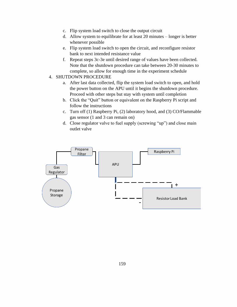
159
c. Flip system load switch to close the output circuit
d. Allow system to equilibrate for at least 20 minutes – longer is better
whenever possible
e. Flip system load switch to open the circuit, and reconfigure resistor
bank to next intended resistance value
f. Repeat steps 3c-3e until desired range of values have been collected.
Note that the shutdown procedure can take between 20-30 minutes to
complete, so allow for enough time in the experiment schedule
4. SHUTDOWN PROCEDURE
a. After last data collected, flip the system load switch to open, and hold
the power button on the APU until it begins the shutdown procedure.
Proceed with other steps but stay with system until completion
b. Click the “Quit” button or equivalent on the Raspberry Pi script and
follow the instructions
c. Turn off (1) Raspberry Pi, (2) laboratory hood, and (3) CO/Flammable
gas sensor (1 and 3 can remain on)
d. Close regulator valve to fuel supply (screwing “up”) and close main
outlet valve

160
13.4 SOFC APU Experiment Data
The following Table 8 contains information regarding the characteristics of each
experiment. The hand-collected experiments from November 11, 2017 are included
with their limited information. In addition, plots showing the most relevant raw data
for each run are provided.
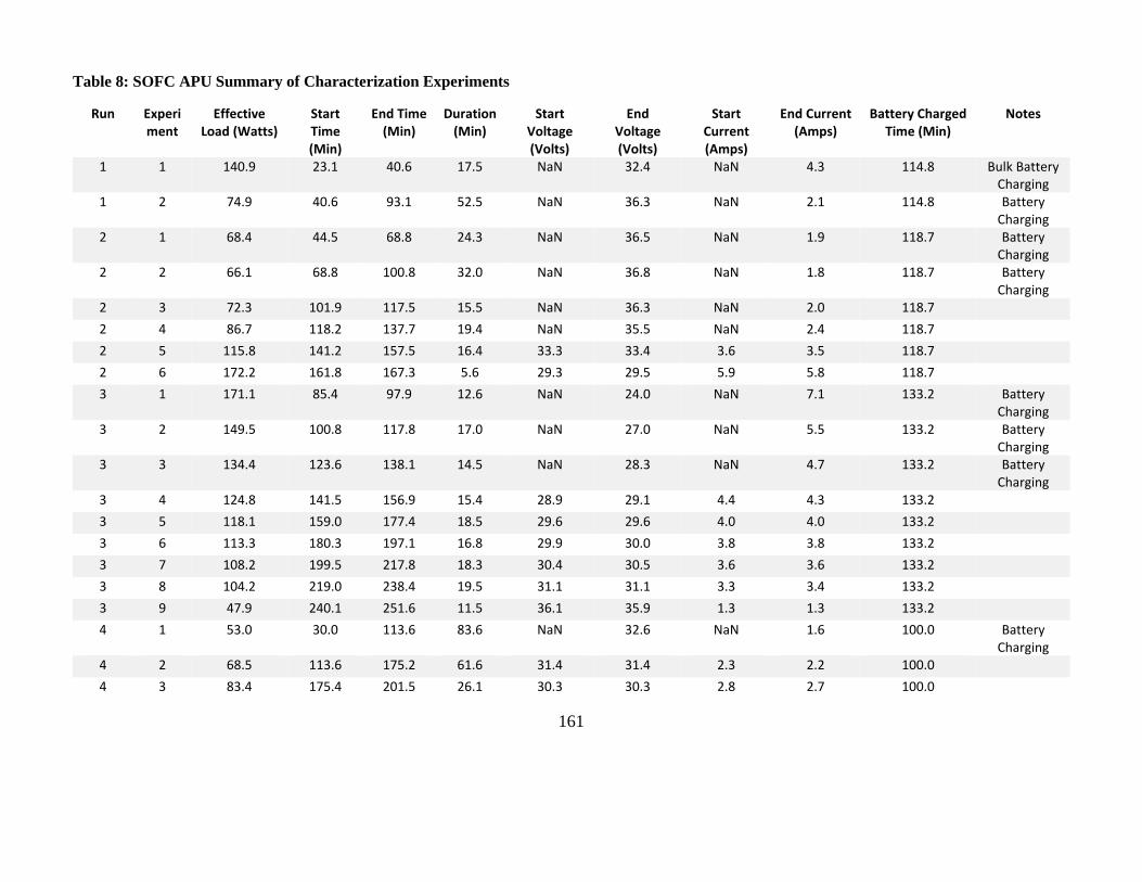
161
Table 8: SOFC APU Summary of Characterization Experiments
Run Experiment
Effective Load (Watts)
Start Time (Min)
End Time (Min)
Duration (Min)
Start Voltage (Volts)
End Voltage (Volts)
Start Current (Amps)
End Current (Amps)
Battery Charged Time (Min)
Notes
1 1 140.9 23.1 40.6 17.5 NaN 32.4 NaN 4.3 114.8 Bulk Battery Charging
1 2 74.9 40.6 93.1 52.5 NaN 36.3 NaN 2.1 114.8 Battery Charging
2 1 68.4 44.5 68.8 24.3 NaN 36.5 NaN 1.9 118.7 Battery Charging
2 2 66.1 68.8 100.8 32.0 NaN 36.8 NaN 1.8 118.7 Battery Charging
2 3 72.3 101.9 117.5 15.5 NaN 36.3 NaN 2.0 118.7
2 4 86.7 118.2 137.7 19.4 NaN 35.5 NaN 2.4 118.7
2 5 115.8 141.2 157.5 16.4 33.3 33.4 3.6 3.5 118.7
2 6 172.2 161.8 167.3 5.6 29.3 29.5 5.9 5.8 118.7
3 1 171.1 85.4 97.9 12.6 NaN 24.0 NaN 7.1 133.2 Battery Charging
3 2 149.5 100.8 117.8 17.0 NaN 27.0 NaN 5.5 133.2 Battery Charging
3 3 134.4 123.6 138.1 14.5 NaN 28.3 NaN 4.7 133.2 Battery Charging
3 4 124.8 141.5 156.9 15.4 28.9 29.1 4.4 4.3 133.2
3 5 118.1 159.0 177.4 18.5 29.6 29.6 4.0 4.0 133.2
3 6 113.3 180.3 197.1 16.8 29.9 30.0 3.8 3.8 133.2
3 7 108.2 199.5 217.8 18.3 30.4 30.5 3.6 3.6 133.2
3 8 104.2 219.0 238.4 19.5 31.1 31.1 3.3 3.4 133.2
3 9 47.9 240.1 251.6 11.5 36.1 35.9 1.3 1.3 133.2
4 1 53.0 30.0 113.6 83.6 NaN 32.6 NaN 1.6 100.0 Battery Charging
4 2 68.5 113.6 175.2 61.6 31.4 31.4 2.3 2.2 100.0
4 3 83.4 175.4 201.5 26.1 30.3 30.3 2.8 2.7 100.0
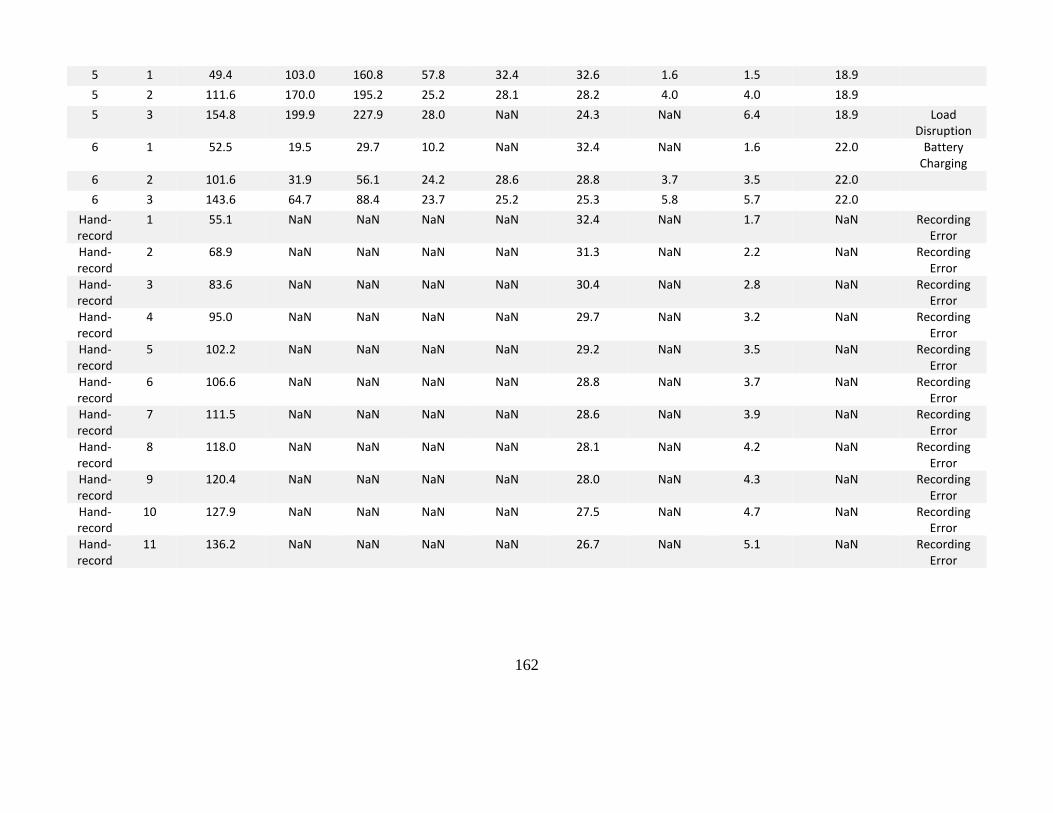
162
5 1 49.4 103.0 160.8 57.8 32.4 32.6 1.6 1.5 18.9
5 2 111.6 170.0 195.2 25.2 28.1 28.2 4.0 4.0 18.9
5 3 154.8 199.9 227.9 28.0 NaN 24.3 NaN 6.4 18.9 Load Disruption
6 1 52.5 19.5 29.7 10.2 NaN 32.4 NaN 1.6 22.0 Battery Charging
6 2 101.6 31.9 56.1 24.2 28.6 28.8 3.7 3.5 22.0
6 3 143.6 64.7 88.4 23.7 25.2 25.3 5.8 5.7 22.0
Hand-record
1 55.1 NaN NaN NaN NaN 32.4 NaN 1.7 NaN Recording Error
Hand-record
2 68.9 NaN NaN NaN NaN 31.3 NaN 2.2 NaN Recording Error
Hand-record
3 83.6 NaN NaN NaN NaN 30.4 NaN 2.8 NaN Recording Error
Hand-record
4 95.0 NaN NaN NaN NaN 29.7 NaN 3.2 NaN Recording Error
Hand-record
5 102.2 NaN NaN NaN NaN 29.2 NaN 3.5 NaN Recording Error
Hand-record
6 106.6 NaN NaN NaN NaN 28.8 NaN 3.7 NaN Recording Error
Hand-record
7 111.5 NaN NaN NaN NaN 28.6 NaN 3.9 NaN Recording Error
Hand-record
8 118.0 NaN NaN NaN NaN 28.1 NaN 4.2 NaN Recording Error
Hand-record
9 120.4 NaN NaN NaN NaN 28.0 NaN 4.3 NaN Recording Error
Hand-record
10 127.9 NaN NaN NaN NaN 27.5 NaN 4.7 NaN Recording Error
Hand-record
11 136.2 NaN NaN NaN NaN 26.7 NaN 5.1 NaN Recording Error
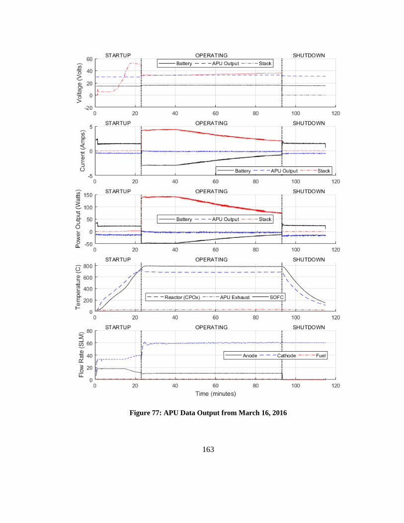
163
Figure 77: APU Data Output from March 16, 2016
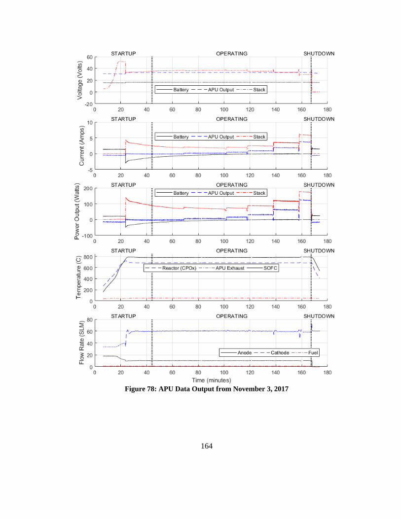
164
Figure 78: APU Data Output from November 3, 2017
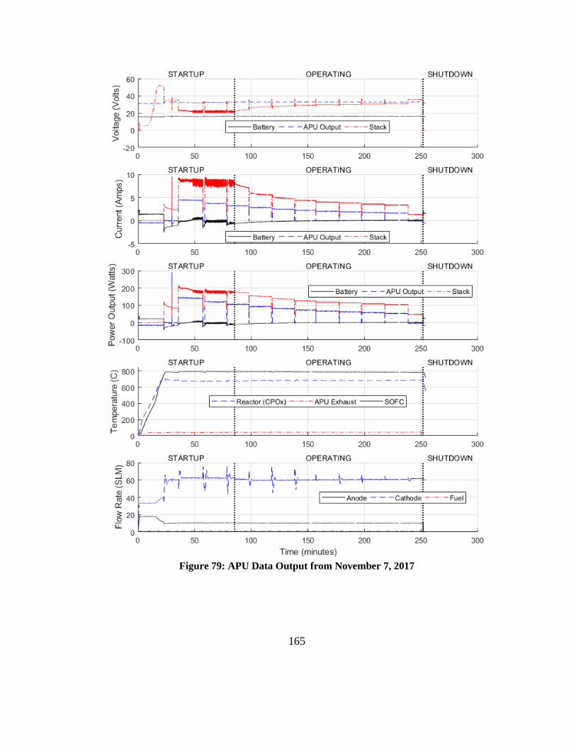
165
Figure 79: APU Data Output from November 7, 2017
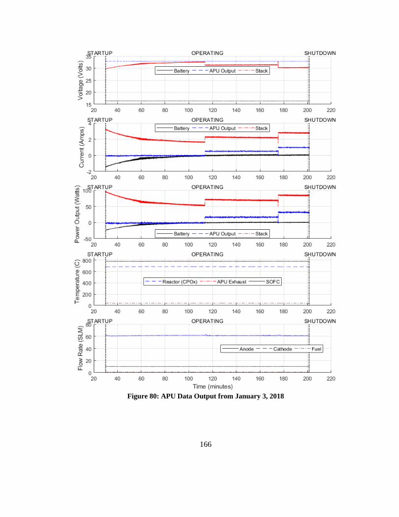
166
Figure 80: APU Data Output from January 3, 2018
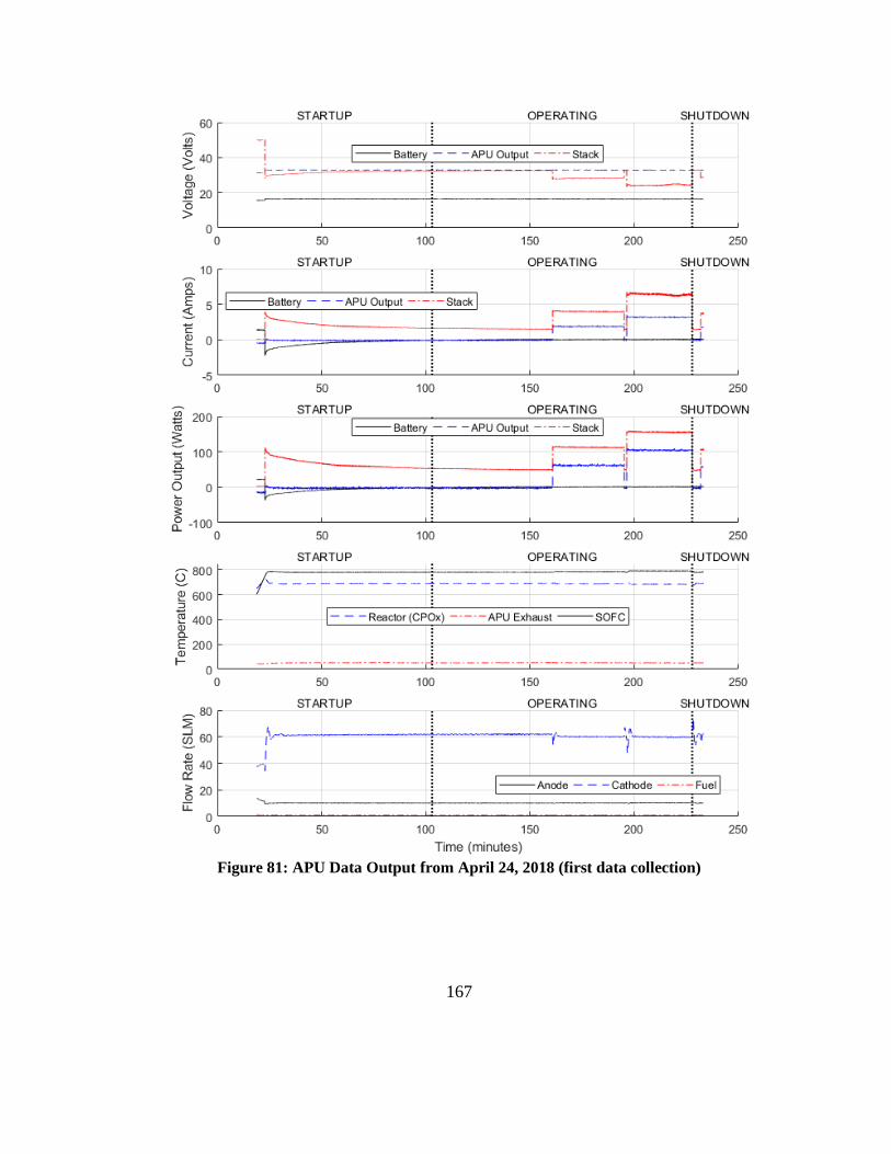
167
Figure 81: APU Data Output from April 24, 2018 (first data collection)
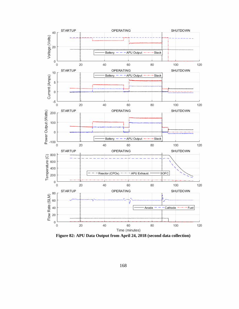
168
Figure 82: APU Data Output from April 24, 2018 (second data collection)

169
14 Bibliography
[1] D. F. Waters, “Modeling of Gas Turbine - Solid Oxide Fuel Cell Systems For
Combined Propulsion and Power on Aircraft,” University of Maryland, 2015.
[2] K. Rajashekara, “More electric aircraft trends [Technology Leaders],” IEEE
Electrif. Mag., vol. 2, no. 4, 2014.
[3] National Aeronautics and Space Administration, “NEW AVIATION
HORIZONS INITIATIVE and Complementary Investments,” 2017.
[4] L. M. Pratt, S. Vannoy, and C. P. Cadou, “Development of an Engine-
Integrated Fuel Cell Concept Demonstrator: Initial System Sizing,” 52nd
AIAA/SAE/ASEE Jt. Propuls. Conf., pp. 1–14, 2016.
[5] P. Jackson, K. Munson, and L. Peacock, “IHS Jane’s All the World’s Aircraft:
Development & Production.” IHS Global, Inc., Alexandria, VA, 2014.
[6] M. Daly and M. Streetly, “IHS Jane’s All the World’s Aircraft: Unmanned,”
Alexandria, VA.
[7] S. W. Ashcraft, A. S. Padron, K. a Pascioni, G. W. Stout Jr., and D. L. Huff,
“Review of Propulsion Technologies for N+3 Subsonic Vehicle Concepts,” no.
October, p. 38, 2011.
[8] R. Royce, Jet Engine, 5th ed. John Wiley & Sons, 2015.
[9] L. R. Radovic and H. H. Schobert, “Chapter 4: Efficiency of Energy
Conversion,” in Energy and Fuels in Society: Analysis of Bills and Media
Reports, 2nd ed., no. 1, New York: McGraw-Hill, 1997, pp. 53–76.
[10] X. Li, Principles of Fuel Cells, 1st ed. New York: Taylor & Francis, 2006.
[11] A. J. Head, “Performance Trends of High-Bypass Civil Turbofans,” 2015.
[12] K. Flittie and B. Curtin, “Pathfinder solar-powered aircraft flight
performance,” 23rd Atmos. Flight Mech. Conf., 1998.
[13] B. Scrosati and J. Garche, “Lithium batteries: Status, prospects and future,” J.
Power Sources, vol. 195, no. 9, pp. 2419–2430, 2010.
[14] W. Ng and A. Datta, “Development of Propulsion System Models for Electric-
VTOL Aircraft,” in 2018 AIAA Aerospace Sciences Meeting, 2018.
[15] M. Yassine and D. Fabris, “Performance of Commercially Available
Supercapacitors,” Energies, vol. 10, no. 9, p. 1340, Sep. 2017.
[16] P. G. Hill and C. R. Peterson, Mechanics and Thermodynamics of Propulsion,
2nd ed. Reading, MA: Addison-Wesley, 1992.
[17] D. F. Waters and C. P. Cadou, “Engine-integrated solid oxide fuel cells for
170
efficient electrical power generation on aircraft,” J. Power Sources, vol. 284,
pp. 588–605, Jun. 2015.
[18] M. Henke et al., “Effect of pressure variation on power density and efficiency
of solid oxide fuel cells,” Electrochim. Acta, vol. 66, pp. 158–163, Apr. 2012.
[19] J. H. Yi and T. S. Kim, “Effects of fuel utilization on performance of
SOFC/gas turbine combined power generation systems,” J. Mech. Sci.
Technol., vol. 31, no. 6, pp. 3091–3100, Jun. 2017.
[20] F. Calise, M. Dentice d’ Accadia, L. Vanoli, and M. R. von Spakovsky,
“Single-level optimization of a hybrid SOFC–GT power plant,” J. Power
Sources, vol. 159, no. 2, pp. 1169–1185, Sep. 2006.
[21] Y. HASELI, I. DINCER, and G. NATERER, “Thermodynamic modeling of a
gas turbine cycle combined with a solid oxide fuel cell,” Int. J. Hydrogen
Energy, vol. 33, no. 20, pp. 5811–5822, Oct. 2008.
[22] A. Abbasi and Z. Jiang, “Multidisciplinary modeling and simulation of a fuel
cell/gas turbine hybrid power system,” in 2009 IEEE Power & Energy Society
General Meeting, 2009, pp. 1–7.
[23] S. H. Chan, H. K. Ho, and Y. Tian, “Modelling of simple hybrid solid oxide
fuel cell and gas turbine power plant,” J. Power Sources, vol. 109, no. 1, pp.
111–120, Jun. 2002.
[24] J. Palsson, A. Selimovic, and L. Sjunnesson, “Combined solid oxide fuel cell
and gas turbine systems for efficient power and heat generation,” J. Power
Sources, vol. 86, no. 1–2, pp. 442–448, Mar. 2000.
[25] P. Costamagna, L. Magistri, and A. F. Massardo, “Design and part-load
performance of a hybrid system based on a solid oxide fuel cell reactor and a
micro gas turbine,” J. Power Sources, vol. 96, no. 2, pp. 352–368, Jun. 2001.
[26] T. LIM et al., “Operating characteristics of a 5kW class anode-supported
planar SOFC stack for a fuel cell/gas turbine hybrid system,” Int. J. Hydrogen
Energy, Jan. 2008.
[27] T. Suther, A. S. Fung, M. Koksal, and F. Zabihian, “Effects of operating and
design parameters on the performance of a solid oxide fuel cell-gas turbine
system,” Int. J. Energy Res., vol. 35, no. 7, pp. 616–632, Jun. 2011.
[28] Y. Zhao, J. Sadhukhan, A. Lanzini, N. Brandon, and N. Shah, “Optimal
integration strategies for a syngas fuelled SOFC and gas turbine hybrid,” J.
Power Sources, vol. 196, no. 22, pp. 9516–9527, Nov. 2011.
[29] L. Leto, C. Dispenza, A. Moreno, and A. Calabrò, “Simulation model of a
molten carbonate fuel cell–microturbine hybrid system,” Appl. Therm. Eng.,
vol. 31, no. 6–7, pp. 1263–1271, May 2011.
171
[30] A. Buonomano, F. Calise, M. D. D’Accadia, A. Palombo, and M. Vicidomini,
“Hybrid solid oxide fuel cells-gas turbine systems for combined heat and
power: A review,” Appl. Energy, vol. 156, pp. 32–85, 2015.
[31] M. A. Azizi and J. Brouwer, “Progress in solid oxide fuel cell-gas turbine
hybrid power systems: System design and analysis, transient operation,
controls and optimization,” Appl. Energy, vol. 215, no. August 2017, pp. 237–
289, Apr. 2018.
[32] J. H. Yi, J. H. Choi, and T. S. Kim, “Comparative evaluation of viable options
for combining a gas turbine and a solid oxide fuel cell for high performance,”
Appl. Therm. Eng., vol. 100, pp. 840–848, 2016.
[33] M. Rokni, “Performance Comparison on Repowering of a Steam Power Plant
with Gas Turbines and Solid Oxide Fuel Cells,” Energies, vol. 9, no. 6, p. 399,
May 2016.
[34] Z. Hajabdollahi and P.-F. Fu, “Multi-objective based configuration
optimization of SOFC-GT cogeneration plant,” Appl. Therm. Eng., vol. 112,
pp. 549–559, Feb. 2017.
[35] T. Choudhary and Sanjay, “Thermodynamic assessment of advanced SOFC-
blade cooled gas turbine hybrid cycle,” Int. J. Hydrogen Energy, vol. 42, no.
15, pp. 10248–10263, Apr. 2017.
[36] P. Saisirirat, “The Solid Oxide Fuel Cell (SOFC) and Gas Turbine (GT) Hybrid
System Numerical Model,” Energy Procedia, vol. 79, pp. 845–850, Nov. 2015.
[37] J. H. Yi, J. H. Choi, and T. S. Kim, “A Comparative Study on the Options in
Combining Solid Oxide Fuel Cell with Gas Turbine,” in Proceedings of the
ASME Turbo Expo 2015: Turbine Technical Conference and Exposition, 2015.
[38] J. Pirkandi, M. Mahmoodi, and M. Ommian, “An optimal configuration for a
solid oxide fuel cell-gas turbine (SOFC-GT) hybrid system based on thermo-
economic modelling,” J. Clean. Prod., vol. 144, pp. 375–386, Feb. 2017.
[39] S. F. Sghaier, T. Khir, and A. Ben Brahim, “Energetic and exergetic parametric
study of a SOFC-GT hybrid power plant,” Int. J. Hydrogen Energy, vol. 43,
no. 6, pp. 3542–3554, Feb. 2018.
[40] Z. Dang, H. Zhao, and G. Xi, “Conceptual Design and Performance Analysis
of SOFC/Micro Gas Turbine Hybrid Distributed Energy System,” J. Fuel Cell
Sci. Technol., vol. 12, no. 3, p. 031003, Jun. 2015.
[41] E. A. Valencia, V. Hidalgo, L. Panagiotis, D. Nalianda, R. Singh, and C. Liu,
“Design Point Analysis of an Hybrid Fuel Cell Gas Turbine Cycle for
Advanced Distributed Propulsion Systems,” in 51st AIAA/SAE/ASEE Joint
Propulsion Conference, 2015.
[42] V. A. Chakravarthula, R. A. Roberts, and M. Wolff, “Dynamic Model of Solid
172
Oxide Fuel Cell Integrated with Fan and Exhaust Nozzle,” in 14th
International Energy Conversion Engineering Conference, 2016, pp. 1–14.
[43] K. Okai, T. Himeno, T. Watanabe, H. Nomura, and T. Tagashira,
“Investigation of FC/GT Hybrid Core in Electrical Propulsion for Fan
Aircraft,” in 51st AIAA/SAE/ASEE Joint Propulsion Conference, 2015, pp. 1–
2.
[44] K. Okai, T. Himeno, T. Watanabe, H. Nomura, T. Tagashira, and A.
Nishizawa, “Potential of Aircraft Electric Propulsion with SOFC/GT Hybrid
Core,” in 52nd AIAA/SAE/ASEE Joint Propulsion Conference, 2016, pp. 1–14.
[45] K. Okai, H. Nomura, T. Tagashira, and A. Nishizawa, “Effects of Fuel Type on
Aircraft Electric Propulsion with SOFC/GT Hybrid Core,” in 53rd
AIAA/SAE/ASEE Joint Propulsion Conference, 2017, no. July, pp. 1–13.
[46] S. E. Veyo, L. A. Shockling, J. T. Dederer, J. E. Gillett, and W. L. Lundberg,
“Tubular Solid Oxide Fuel Cell/Gas Turbine Hybrid Cycle Power Systems:
Status,” J. Eng. Gas Turbines Power, vol. 124, no. 4, p. 845, 2002.
[47] R. J. Braun, M. Gummalla, and J. Yamanis, “System Architectures for Solid
Oxide Fuel Cell-Based Auxiliary Power Units in Future Commercial Aircraft
Applications,” J. Fuel Cell Sci. Technol., vol. 6, no. 3, p. 031015, 2009.
[48] S. Eelman, I. del Pozo y de Poza, and T. Krieg, “Fuel Cell APU’s in
Commercial Aircraft – an Assessment of SOFC and PEMFC Concepts,” 24th
Int. Congr. Aeronaut. Sci. (IC, pp. 1–10, 2004.
[49] J. E. Freeh, J. W. Pratt, and J. Brouwer, “Development of a Solid-Oxide Fuel
Cell/Gas Turbine Hybrid System Model for Aerospace Applications,” in
Volume 7: Turbo Expo 2004, 2004, no. May 2004, pp. 371–379.
[50] J. E. Freeh, C. J. Steffen, and L. M. Larosiliere, “Off-Design Performance
Analysis of a Solid-Oxide Fuel Cell/Gas Turbine Hybrid for Auxiliary
Aerospace Power,” in 3rd International Conference on Fuel Cell Science,
Engineering and Technology, 2005, vol. 2005, no. December 2005, pp. 265–
272.
[51] K. Rajashekara, J. Grieve, and D. Daggett, “Solid Oxide Fuel Cell/Gas Turbine
Hybrid APU System for Aerospace Applications,” in Conference Record of the
2006 IEEE Industry Applications Conference Forty-First IAS Annual Meeting,
2006, vol. 5, pp. 2185–2192.
[52] K. Rajashekara, J. Grieve, and David Dagget, “Hybrid Fuel Cell Power in
Aircraft,” IEEE Industry Applications Magazine, vol. 14, pp. 54–60, 2008.
[53] C. J. Steffen, J. E. Freeh, and L. M. Larosiliere, “Solid Oxide Fuel Cell/Gas
Turbine Hybrid Cycle Technology for Auxiliary Aerospace Power,” in Volume
5: Turbo Expo 2005, 2005, no. May 2005, pp. 253–260.

173
[54] A. Himansu, J. E. Freeh, C. J. Steffen, R. T. Tornabene, and X.-Y. J. Wang,
“Hybrid Solid Oxide Fuel Cell/Gas Turbine System for High Altitude Long
Endurance Aerospace Missions,” in ASME 2006 Fourth International
Conference on Fuel Cell Science, Engineering and Technology, Parts A and B,
2006, vol. 2006, no. May 2006, pp. 573–583.
[55] P. AGUIAR, D. BRETT, and N. BRANDON, “Solid oxide fuel cell/gas
turbine hybrid system analysis for high-altitude long-endurance unmanned
aerial vehicles,” Int. J. Hydrogen Energy, vol. 33, no. 23, pp. 7214–7223, Dec.
2008.
[56] M. K. Bradley and C. K. Droney, “Subsonic Ultra Green Aircraft Research :
Phase I Final Report,” 2011.
[57] M. K. Bradley and C. K. Droney, “Subsonic Ultra Green Aircraft Research
Phase II: N+4 Advanced Concept Development,” 2012.
[58] S. M. Jones, “An introduction to thermodynamic performance analysis of
aircraft gas turbine engine cycles using the numerical propulsion system
simulation code,” no. March, 2007.
[59] Mason E. A. and A. P. Malinauskas, Gas transport in porous media : the
dusty-gas model / E.A. Mason and A.P. Malinauskas. Elsevier Scientific Pub.
Co Amsterdam ; New York, 1983.
[60] D. F. Waters, S. Vannoy, and C. P. Cadou, “Influence of Flow Path
Configuration on the Performance of Hybrid Turbine - Solid Oxide Fuel Cell
Systems for Aircraft Propulsion and Power,” in 51st AIAA/SAE/ASEE Joint
Propulsion Conference, 2015.
[61] S. Vannoy and C. P. Cadou, “Development and Validation of an NPSS Model
of a Small Turbojet Engine,” in 52nd AIAA/SAE/ASEE Joint Propulsion
Conference, 2016.
[62] S. Vannoy, “Development and Validation of an NPSS Model of a Small
Turbojet Engine,” University of Maryland College Park, 2017.
[63] B. Campbell, S. Crase, and B. Sims, “Review of Fuel Cell Technologies for
Military Land Vehicles,” Fisherman’s Bend, 2014.
[64] “NPSS TM REFPROP Thermodynamic Property Package User Guide,” 2012.
[65] “NPSS Developer’s Guide.” 2008.
[66] NPSS User Guide, Rev. 4., vol. 01. Cleveland: Ohio Aerospace Institute, 2012.
[67] “NPSS Customer Deck User’s Guide.” 2008.
[68] D. F. Waters and C. P. Cadou, “Optimization of Gas Turbine - Solid Oxide
Fuel Cell Systems for Aircraft Power Generation,” in 53rd AIAA Aerospace
Sciences Meeting, 2015, no. January, pp. 1–15.
174
[69] C. Kelley, Solving Nonlinear Equations with Newton’s Method. Philadelphia:
Society for Industrial and Applied Mathematics, 2003.
[70] S. Gordon and B. J. McBride, “Computer Program for Calculation of Complex
Chemical Equilibrium Compositions and Applications, NASA RP-1311.”
NASA, 1994.
[71] “NPSS Reference Sheets,” Cleveland, 2008.
[72] F.-P. Nagel, “Electricity from wood through the combination of gasification
and solid oxide fuel cells Systems analysis and Proof-of-concept,” ETH
Zurich, 2008.
[73] A. H. Lefebvre and D. R. Ballal, Gas Turbine Combustion: Alternative Fuels
and Emissions, Third Edition, 3rd ed. Taylor & Francis, 2010.
[74] Y. S. Muzychka and M. M. Yovanovich, “Pressure Drop in Laminar
Developing Flow in Noncircular Ducts: A Scaling and Modeling Approach,” J.
Fluids Eng., vol. 131, no. 11, p. 111105, 2009.
[75] Y. S. Muzychka and M. M. Yovanovich, “Laminar Forced Convection Heat
Transfer in the Combined Entry Region of Non-Circular Ducts,” J. Heat
Transfer, vol. 126, no. 1, p. 54, 2004.
[76] F. P. Incroprera, D. P. DeWitt, T. L. Bergman, and A. S. Lavine,
Fundamentals of Heat and Mass Transfer, 6th ed. Hoboken, NJ: John Wiley &
Sons, Inc., 2007.
[77] H. Zhu and R. J. Kee, “A general mathematical model for analyzing the
performance of fuel-cell membrane-electrode assemblies,” J. Power Sources,
vol. 117, no. 1–2, pp. 61–74, May 2003.
[78] H. Zhu, R. Kee, and G. Jackson, “Solid Oxide Fuel Cells Using Syngas,” in
Synthesis Gas Combustion, CRC Press, 2009, pp. 329–374.
[79] X. B. Zhu et al., “A direct flame solid oxide fuel cell for potential combined
heat and power generation,” Int. J. Hydrogen Energy, vol. 37, no. 10, pp.
8621–8629, 2012.
[80] H. Zhu and R. J. Kee, “Modeling Distributed Charge-Transfer Processes in
SOFC Membrane Electrode Assemblies,” J. Electrochem. Soc., vol. 155, no. 7,
p. B715, 2008.
[81] H. Zhu, R. J. Kee, V. M. Janardhanan, O. Deutschmann, and D. G. Goodwin,
“Modeling Elementary Heterogeneous Chemistry and Electrochemistry in
Solid-Oxide Fuel Cells,” J. Electrochem. Soc., vol. 152, no. 12, p. A2427,
2005.
[82] R. J. Kee, H. Zhu, A. M. Sukeshini, and G. S. Jackson, “Solid Oxide Fuel
Cells: Operating Principles, Current Challenges, and the Role of Syngas,”
175
Combust. Sci. Technol., vol. 180, no. 6, pp. 1207–1244, May 2008.
[83] R. J. Kee, H. Zhu, and D. G. Goodwin, “Solid-oxide fuel cells with
hydrocarbon fuels,” Proc. Combust. Inst., vol. 30, no. 2, pp. 2379–2404, Jan.
2005.
[84] H. Zhu and R. J. Kee, “Thermodynamics of SOFC efficiency and fuel
utilization as functions of fuel mixtures and operating conditions,” J. Power
Sources, vol. 161, no. 2, pp. 957–964, Oct. 2006.
[85] H. Zhu and R. J. Kee, “The influence of current collection on the performance
of tubular anode-supported SOFC cells,” J. Power Sources, vol. 169, no. 2, pp.
315–326, Jun. 2007.
[86] E. Onat and G. W. Klees, “A method to estimate weight and dimensions of
large and small gas turbine engines,” 1979.
[87] V. Sanghi, S. K. Kumar, S. K. Sane, and V. Sundararajan, “Preliminary
Estimation of Engine Gas-Flow-Path Size and Weight,” J. Propuls. Power,
vol. 14, no. 2, pp. 208–214, 1998.
[88] D. Raymer, Aircraft Design: A Conceptual Approach, 2nd ed. Washington,
DC: American Institute of Aeronautics and Astronautics, Inc., 2012.
[89] C. C. CIEPLUCH, D. Y. DAVIS, and D. E. GRAY, “Results of NASA’s
Energy Efficient Engine Program,” J. Propuls. Power, vol. 3, no. 6, pp. 560–
568, Nov. 1987.
[90] “Ultra Electronics AMI fuel cells for UAVs, critical military tech,” Fuel Cells
Bull., vol. 2013, no. 7, p. 4, Jul. 2013.
[91] M. Hanasaki et al., “SOFC Durability against Standby and Shutdown
Cycling,” vol. 161, no. 9, pp. 850–860, 2014.
[92] L. Mastropasqua, S. Campanari, and J. Brouwer, “Solid oxide fuel cell short
stack performance testing - Part A: Experimental analysis and Μ-combined
heat and power unit comparison,” J. Power Sources, vol. 371, pp. 225–237,
2017.
[93] R. L. Edwards and A. Demuren, “Regression analysis of PEM fuel cell
transient response,” Int. J. Energy Environ. Eng., vol. 7, no. 3, pp. 329–341,
2016.
[94] P. G. Batterton, “Energy Efficient Engine Program Contributions to Aircraft
Fuel Conservation,” in Aviation Fuel Conservation Symposium, 1984.
[95] J. D. Mattingly, Elements of Propulsion: Gas Turbines and Rockets. Reston
,VA: American Institute of Aeronautics and Astronautics, 2006.
[96] N. M. Sammes, R. Bove, and J. Pusz, “Solid Oxide Fuel Cells,” in Fuel Cell
Technology: Reaching Towards Commercialization, N. Sammes, Ed. London:

176
Springer London, 2006, pp. 1–26.
[97] G. P. Sutton and O. Biblarz, Rocket Propulsion Elements. John Wiley & Sons,
2010.
[98] S. G. Chalk and J. F. Miller, “Key challenges and recent progress in batteries,
fuel cells, and hydrogen storage for clean energy systems,” J. Power Sources,
vol. 159, no. 1, pp. 73–80, Sep. 2006.
[99] N. Sammes, Ed., Fuel Cell Technology. London: Springer London, 2006.


![Solid Oxide Fuel Cell/Gas Turbine Hybrid Cycle Technology ...Fuel Cell (SOFC) gas turbine hybrid system demonstration on a ~200 kW system [2]. This 200 to 500 kW power range overlaps](https://img.pdfslide.us/doc/110x75/6129f38f7735990dd676cd4b/solid-oxide-fuel-cellgas-turbine-hybrid-cycle-technology-fuel-cell-sofc-gas.jpg)