Embed Size (px)
Citation preview

ABSTRACT
Title of Thesis: DEVELOPMENT AND VALIDATION OF AN
NPSS MODEL OF A SMALL TURBOJET
ENGINE.
Stephen Michael Vannoy,
Master of Science, 2017
Thesis Directed By: Associate Professor, Christopher P. Cadou,
Department of Aerospace Engineering
Recent studies have shown that integrated gas turbine engine (GT)/solid oxide fuel
cell (SOFC) systems for combined propulsion and power on aircraft offer a promising
method for more efficient onboard electrical power generation. However, it appears
that nobody has actually attempted to construct a hybrid GT/SOFC prototype for
combined propulsion and electrical power generation. This thesis contributes to this
ambition by developing an experimentally validated thermodynamic model of a small
gas turbine (~230 N thrust) platform for a bench-scale GT/SOFC system. The
thermodynamic model is implemented in a NASA-developed software environment
called Numerical Propulsion System Simulation (NPSS). An indoor test facility was
constructed to measure the engine’s performance parameters: thrust, air flow rate,
fuel flow rate, engine speed (RPM), and all axial stage stagnation temperatures and
pressures. The NPSS model predictions are compared to the measured performance
parameters for steady state engine operation.

DEVELOPMENT AND VALIDATION OF AN NPSS MODEL OF A SMALL
TURBOJET ENGINE.
By
Stephen Michael Vannoy
Thesis submitted to the Faculty of the Graduate School of the
University of Maryland, College Park, in partial fulfillment
of the requirements for the degree of
Master of Science
2017
Advisory Committee:
Associate Professor Christopher P. Cadou, Chair
Associate Professor Stuart Laurence
Associate Professor Kenneth Yu

© Copyright by
Stephen Michael Vannoy
2017

ii
Dedication
To my family for always providing me with
unconditional love and support.

iii
Acknowledgements
First and foremost, I would like to thank my advisor, Dr. Chris Cadou, for
providing me the opportunity to work on this project and teaching me there is always
more than one way to approach to a problem.
Thank you to the United Sates Navy and particularly the Office of Naval
Research for financially supporting this project.
Thank you to Dan Waters for teaching me NPSS in the beginning and
providing me assistance with the software throughout the project.
Thank you to Prof. Harald Funke at Aachen University of Applied Sciences in
Aachen, Germany for providing preliminary performance data for the AMT Olympus
engine prior to construction of our test facility.
I would also like to thank my labmates for creating a fun and enjoyable work
environment. In particular, I would like to thank: Daanish Maqbool, Colin Adamson,
Chandan Kittur, Andrew Ceruzzi, Wiam Attar, Lucas Pratt, and Branden Chiclana.
Lastly, I would like to thank the University of Maryland Police Department
and College Park Fire Department for not shutting down my experiments after
triggering the smoke alarms for two consecutive nights in one week during the initial
testing phases.

iv
Table of Contents
Dedication ..................................................................................................................... ii
Acknowledgements ...................................................................................................... iii Table of Contents ......................................................................................................... iv List of Tables .............................................................................................................. vii List of Figures ............................................................................................................ viii Nomenclature ................................................................................................................ x
Chapter 1: Introduction ................................................................................................. 1 1.1 Motivation ........................................................................................................... 1
1.1.1 Electric Power on Aircraft .............................................................................1 1.1.2 Role of Liquid Hydrocarbons ........................................................................3 1.1.3 Fuel Consumption .........................................................................................5
1.2 Turbojets .............................................................................................................. 7
1.2.1 Fundamentals of Turbojet Operation .............................................................7 1.2.2 Applications of Small Turbojet Engines .....................................................11
1.3 Fuel Cells ........................................................................................................... 13 1.3.1 Fundamentals of Fuel Cell Operation..........................................................13 1.3.2 Applications of Fuel Cells in Aircraft .........................................................21
1.4 Gas Turbine/Solid Oxide Fuel Cell Hybridization ............................................ 22 1.4.1 Advantages of System Coupling .................................................................22 1.4.2 Challenges ...................................................................................................24
1.4.3 Literature Review of GT/SOFC Systems ....................................................25 1.5 Objectives .......................................................................................................... 28
1.6 Previous Work ................................................................................................... 28
1.7 Approach ........................................................................................................... 30
Chapter 2: Engine Selection........................................................................................ 31 Chapter 3: NPSS Engine Model ................................................................................. 35
3.1 Overview of NPSS ............................................................................................ 35 3.2 Olympus Engine Model Components ............................................................... 39
3.2.1 Ambient Element .........................................................................................39
3.2.2 Burner Element ............................................................................................40 3.2.3 Compressor Element ...................................................................................41
3.2.4 Duct Element ...............................................................................................43 3.2.5 Flow End Element .......................................................................................44 3.2.6 Fuel Start Element .......................................................................................44 3.2.7 Inlet Element ...............................................................................................45 3.2.8 Inlet Start Element .......................................................................................45
3.2.9 Nozzle Element ...........................................................................................46 3.2.10 Shaft Element ............................................................................................49
3.2.11 Turbine Element ........................................................................................50 3.3 Solution Method ................................................................................................ 52
3.3.1 Numerical Solver .........................................................................................52 3.3.2 Independents and Dependents .....................................................................53
3.4 Cycle Analysis ................................................................................................... 56 Chapter 4: Engine Performance Measurements .......................................................... 59

v
4.1 Test Facility Design .......................................................................................... 59
4.2 Challenges ......................................................................................................... 61 4.3 Measured Quantities .......................................................................................... 66
4.3.1 Thrust ...........................................................................................................66
4.3.2 Air Flow Rate ..............................................................................................69 4.3.3 Fuel Flow Rate ............................................................................................71 4.3.4 Temperatures ...............................................................................................72 4.3.5 Pressures ......................................................................................................73 4.3.6 Engine Speed ...............................................................................................73
4.3.7 Data Acquisition ..........................................................................................74 4.3.8 Summary of Measurements .........................................................................74
4.4 Thermocouple Corrections ................................................................................ 75 4.4.1 Pin Fin Model ..............................................................................................75
4.4.2 Determining the Convective Heat Transfer Coefficient ..............................80 4.4.3 Parameters for the Thermocouple Corrections ............................................80
4.5 Estimating Uncertainty ...................................................................................... 82 4.5.1 Measurement Uncertainty ...........................................................................82
4.5.2 Uncertainties in Calculated Results .............................................................83 4.6 Experimental Procedures ................................................................................... 85
4.6.1 Preparing the Engine ...................................................................................85
4.6.2 Preparing the Test Facility...........................................................................85 4.6.3 Data Collection ............................................................................................86
4.6.4 Safety ...........................................................................................................87 Chapter 5: Results & Discussion ................................................................................ 89
5.1 Summary of Experiments Performed ................................................................ 89
5.2 Results ............................................................................................................... 89
5.2.1 Axial Stage Pressure & Temperature Comparison ......................................89 5.2.2 Thrust, Fuel Flow Rate, & TSFC Comparison ............................................93 5.2.3 Predicted Air Flow Rate, Exhaust Static Pressure, &Turbine Efficiency ...97
5.2.4 Thrust with & without Air Flow Rate Measurement ................................101 Chapter 6: Conclusions & Future Work ................................................................... 104
6.1 Summary & Key Findings ............................................................................... 104 6.2 Contributions ................................................................................................... 105
6.3 Future Work .................................................................................................... 105 Appendix A: Compressor & Turbine Performance Maps ........................................ 108
A.1 Olympus Compressor Map ............................................................................. 108 A.2 Low Pressure Turbine Map ............................................................................ 109
Appendix B: Details of NPSS Olympus Model ........................................................ 110
B.1 Order of Execution ......................................................................................... 110 B.2 How to Run an NPSS Model .......................................................................... 111
Appendix C: Example NPSS Code ........................................................................... 113 C.1 Turbojet ‘.run’ Run File .................................................................................. 113 C.2 Example ‘.case’ Case File .............................................................................. 114 C.3 Turbojet ‘.mdl’ Model File ............................................................................. 116
Appendix D: Experimental Data ............................................................................... 118 D.1 Performance Data without Air Flow Rate Measurements .............................. 118

vi
D.2 Performance Data with Air Flow Rate Measurements ................................... 119
Bibliography ............................................................................................................. 120

vii
List of Tables
Table 1. Predicted specific energies of different batteries. ............................................4
Table 2. Flight conditions and aircraft specifications for preliminary relative fuel flow
rate calculations. ............................................................................................................6
Table 3. Summary of GT/SOFC literature [1]. ............................................................27
Table 4. Candidate gas turbine platforms. ...................................................................32
Table 5. Locations of the temperature and pressure measurements on the Olympus
engine. ..........................................................................................................................35
Table 6. Independents and dependents for the design case without a turbine map. ....54
Table 7. Independents and dependents for the design case with the low pressure
turbine map. .................................................................................................................54
Table 8. Independents and dependents for off-design cases. .......................................55
Table 9. Full throttle design case parameters for the Olympus engine model. ............57
Table 10. Calibration coefficients for LFE. .................................................................70
Table 11. Summary of measured quantities. ................................................................74
Table 12. Parameters used to calculate T04 and T05 thermocouple corrections. ..........81

viii
List of Figures
Figure 1. Electric power fractions of various commercial, military, and unmanned
aircraft [1]. .....................................................................................................................1
Figure 2. (Top) Relative fuel flow rate vs. electric power fraction; (Bottom) Fuel flow
rate reduction vs. electric power fraction. ......................................................................6
Figure 3. Schematic of a turbojet engine [10]. ...............................................................8
Figure 4. P-v and T-s diagrams of the ideal Brayton cycle. ..........................................8
Figure 5. Clockwise from top left: SubSonex, JB-9 Jetpack, Jetman Dubai Wing Suit,
BQM-74E-Chukar-III. .................................................................................................11
Figure 6. Schematic of a solid oxide fuel cell [1]. .......................................................14
Figure 7. Efficiencies of ideal heat engine and fuel cell vs. temperature [1]. .............17
Figure 8. Clockwise from top left: Ion Tiger, Intelligent Energy’s Quadrotor
Prototype, Boeing’s Experimental FC Aircraft. ..........................................................21
Figure 9. Schematic of a turbojet GT/SOFC [1]. .........................................................22
Figure 10. Engine layout of turbojet GT/SOFC [1]. ....................................................23
Figure 11. AMT Olympus in University Configuration. .............................................33
Figure 12. Schematic diagram of the Olympus and its measurement port locations. ..34
Figure 13. NPSS turbojet model schematic [1]. ..........................................................37
Figure 14. NPSS schematic of AMT Olympus turbojet. .............................................38
Figure 15. Burner element schematic [1]. ....................................................................40
Figure 16. Compressor element schematic [1]. ...........................................................41
Figure 17. Duct element schematic [1]. .......................................................................43
Figure 18. Flow End element schematic [1]. ...............................................................44
Figure 19. Fuel Start element schematic [1]. ...............................................................44
Figure 20. Inlet element schematic [1]. .......................................................................45
Figure 21. Inlet Start element schematic [1]. ...............................................................46
Figure 22. Nozzle element schematic [1]. ...................................................................46
Figure 23. Shaft element schematic [1]. ......................................................................49
Figure 24. Turbine element schematic [1]. ..................................................................50
Figure 25. CAD depiction of engine test facility. ........................................................59
Figure 26. Engine test facility. .....................................................................................60
Figure 27. Custom inlet extension. ..............................................................................61
Figure 28. Engine inlet pressure measurement location. .............................................62
Figure 29. Pressure drop across LFE-plenum-duct as a function of engine speed. .....63
Figure 30. Pressure drop across the LFE as a function of engine speed. .....................64
Figure 31. Thrust calibration curves for different engine speeds during a throttle
sweep............................................................................................................................65
Figure 32. Thrust stand load cell configuration. ..........................................................67
Figure 33. Calibration pulley system. ..........................................................................68

ix
Figure 34. Example thrust stand calibration curve. .....................................................69
Figure 35. Gravimetric fuel weight measurement system. ..........................................71
Figure 36. Fuel weight vs. time for a single engine run at 80% throttle. .....................72
Figure 37. Sheathed thermocouple orientation in flow. ...............................................76
Figure 38. Thermocouple well pin fin model. .............................................................76
Figure 39. Differential sheath element. ........................................................................78
Figure 40. Axial stage pressures (top) and temperatures (bottom) at full throttle
(design case).................................................................................................................90
Figure 41. Percent difference between predicted and measured total pressures (top)
and temperatures (bottom) at various throttle settings. ................................................92
Figure 42. Thrust as a function of corrected RPM (top) and throttle setting (bottom).93
Figure 43. Comparison between measured and predicted corrected RPM. .................94
Figure 44. Fuel flow rate as a function of corrected RPM (top) and throttle setting
(bottom)........................................................................................................................96
Figure 45. TSFC as a function of corrected RPM (top) and throttle setting (bottom). 97
Figure 46. Predicted air flow rate as a function of engine speed. ................................98
Figure 47. Predicted exhaust static pressure as a function of engine speed. ...............99
Figure 48. Predicted turbine efficiency as a function of engine speed. .....................100
Figure 49. Thrust comparison for the case with and without the air flow rate
measurement. .............................................................................................................101
Figure 50. Schematic diagram of the Olympus engine in “University Configuration”
with the extended intake [21]. ....................................................................................103
Figure 51. Olympus engine with the extended intake attached to the inlet [21]. ......103
Figure 52. AMT Olympus compressor performance map. ........................................108
Figure 53. General Electric's low pressure turbine performance map from the Energy
Efficient Engine Program [1]. ....................................................................................109

x
Nomenclature
Abbreviations:
AFC ………… alkaline fuel cell
APU ………… auxiliary power unit
CAD ………… computer-aided drawing
CEA ………… Chemical Equilibrium with Applications
CFD ………… computational fluid dynamics
CPOx ………… catalytic partial oxidation reactor
ECU ………… electronic control unit
EDT ………… electronic data terminal
FAR ………… fuel-to-air ratio
FC ………… fuel cell
GE ………… General Electric
GT ………… gas turbine
LFE ………… laminar flow element
LHC ………… liquid hydrocarbon
MCFC ………… molten carbonate fuel cell
MDF ………… medium-density fiberboard
NASA ………… National Aeronautics and Space Administration
NPSS ………… Numerical Propulsion System Simulation
PAFC ………… phosphoric acid fuel cell
PEMFC ………… proton exchange membrane fuel cell
RPM ………… rotations per minute
SLS ………… sea-level-static
SOFC ………… solid oxide fuel cell
TIT ………… turbine inlet temperature
UAV ………… unmanned air vehicle
UMD ………… University of Maryland
YSZ ………… yttria stabilized zirconia
Symbols:
………… area ………… systematic error ………… total systematic uncertainty ………… drag coefficient at minimum lift ………… minimum lift coefficient ………… nozzle coefficient ………… specific heat capacity at constant pressure
………… force; Faraday constant; thrust ………… acceleration due to gravity; molar specific Gibbs energy ………… Gibbs free energy ………… specific enthalpy; heat transfer coefficient ………… enthalpy

xi
………… conductivity ………… lift induced drag factor ………… length ………… mass ………… mass flow rate ………… effective fin parameter ………… Mach number ………… number/quantity; shaft speed ………… Nusselt number ………… pressure; perimeter ………… Prandtl number ………… flux ………… heat transfer rate ………… fuel heating value
………… gas constant; calculated result
………… mean of a calculated result ………… true value of a calculated result ………… Reynolds number ………… wing area; entropy ………… standard deviation of the sample for a calculated result ………… standard deviation about the mean for a calculated result ………… standard deviation of the sample for a measurement ………… standard deviation about the mean for a measurement ………… temperature; torque ………… thrust specific fuel consumption ………… flow velocity ………… total uncertainty in a calculated result ………… total measurement uncertainty ………… flow or vehicle velocity; specific volume ………… voltage/electric potential
………… volumetric flow rate
………… work rate, power ………… length; measured quantity ………… mean of a measured quantity ………… true measurement value ………… ratio of specific heats ………… pressure correction factor ………… change or difference in/between property values ………… emissivity ………… electric power fraction ………… efficiency ………… sensitivity coefficient; temperature correction factor ………… viscosity ………… pressure ratio ………… density ………… Stefan-Boltzmann constant

xii
Subscripts:
0 ………… initial value; stagnation property
air ………… air property
amb ………… ambient property
c ………… compressor
calc ………… calculated value
carnot ………… Carnot value
corr ………… corrected value
cond ………… conduction
conv ………… convection
des ………… design value
elec ………… electric, electrical
exh ………… exhaust property
exit ………… exit value
f ………… fuel; flow value
free ………… free stream property
fuel ………… fuel property
g ………… gas property
gross ………… gross value
in ………… entrance property
inlet ………… inlet property
input ………… input value
max ………… maximum value
out ………… outlet property
prop ………… propulsion, propulsive
ram ………… ram air; ram compression
s ………… isentropic value; static property
shaft ………… engine shaft
std ………… standard value
R ………… radiation; calculated result
ref ………… reference value
rev ………… reversible
t ………… turbine; total property; thermocouple well tip property
T ………… total property
w ………… wall property
∞ ………… ambient/freestream property

1
Chapter 1: Introduction
1.1 Motivation
1.1.1 Electric Power on Aircraft
The electrical power demands on aircraft are increasing as aircraft subsystems
like climate and flight controls become increasingly electric and more sensors are
added to vehicle platforms. The latter is especially important in the case of unmanned
air vehicles (UAVs). A survey conducted by Waters [1] compares estimates of
electric power fraction ( ) in various commercial, manned military, and unmanned
aircraft (see Figure 1 [1]), where the electric power fraction is defined as the ratio of
electrical power demand to total power demand:
(1)
Figure 1. Electric power fractions of various commercial, military, and unmanned aircraft [1].
In Eq. (1), is the electric power at cruise and is the propulsive
power at cruise. Figure 1 shows that for most modern commercial aircraft, the electric
power fraction is below 4%. The two exceptions are future aircraft with entirely
electric subsystems [2] which have electric power fractions of about 6%. While these
are relatively low, the electric transport aircraft conceptualized by NASA [3] would

2
have electric power fractions well in excess of 50%. Manned military aircraft exhibit
similar electric power fractions to commercial aircraft. Northrop Grumman’s E-2D
Advanced Hawkeye is the exception with . This large electrical power
fraction is due to the Hawkeye’s immense radar system. The most notable
observation from Waters’ survey is that electric power fractions of UAVs are
significantly larger than those in commercial aircraft and most manned military
aircraft. This is because UAVs require substantially larger communications and
sensor payloads. As the applications of UAVs expand in both military and
commercial arenas, so too will the electrical power required to operate these
platforms. Consequently, the efficiency of electric power generation on these aircraft
will have a progressively more important impact on fuel consumption and thus
vehicle range and endurance.
Turbine-powered aircraft generally produce electrical power via mechanical
generators driven by the engine’s shaft or via separate auxiliary power units (APUs)
[4], [5]. These processes for electrical power generation can be relatively inefficient
because fuel passes through the engine’s Brayton cycle to convert chemical potential
energy into mechanical power before generating electrical power. Fuel cells produce
electrical power more efficiently by directly converting the chemical energy stored in
fuel to electrical power. For fuel cell systems without heat recovery cycles,
efficiencies can reach 50-60% [6], whereas efficiencies for gas turbines (GT) are
generally 20-40% [7], [8].

3
1.1.2 Role of Liquid Hydrocarbons
In addition to fuel cells, batteries are being considered as alternative energy
sources for future hybrid/electric propulsion systems [3]. Like fuel cells, batteries
offer reduced emissions, which is a significant driving factor in modern aircraft
design. In Boeing’s SUGAR Volt concept, batteries would power an electric motor
that would be used during taxiing and takeoff to reduce fuel consumption [3].
Unfortunately, batteries have low specific energies, with the latest lithium-ion (Li-
ion) batteries obtaining 0.54-0.9 MJ/kg [3]. A battery with specific energy of at least
2.7 MJ/kg would be required to power the electric assist motor in Boeing’s SUGAR
Volt design [3]. Newer battery technologies such as Lithium-air (or Li-air/Li-O2)
batteries have theoretical specific energy of 12.6 MJ/kg [9] compared to the
theoretical specific energy of 43-48 MJ/kg for liquid hydrocarbon (LHC) aviation
fuel [10].
To compare the practical specific energies of Li-air batteries and LHCs, one
must consider the efficiency of their respective energy conversion systems. Assuming
the efficiency of a gas turbine engine that runs on LHC fuel is 40% ([7], [8]), the
practical specific energy of the fuel is 17.2-19.2 MJ/kg. Conversion efficiencies of
electric motors are much higher than 40%. For example, Siemens recently developed
their SP260D electric aircraft motor which has an efficiency of 95% [11]. With this
efficiency, a Li-air battery powered propulsion system could potentially achieve a
practical specific energy of 11.97 MJ/kg. Thus, the useful energy capacity of Li-air
batteries is comparable to LHCs but still less. In addition, Li-air battery technology is
not expected to achieve its full predicted useful specific energy within the next
4
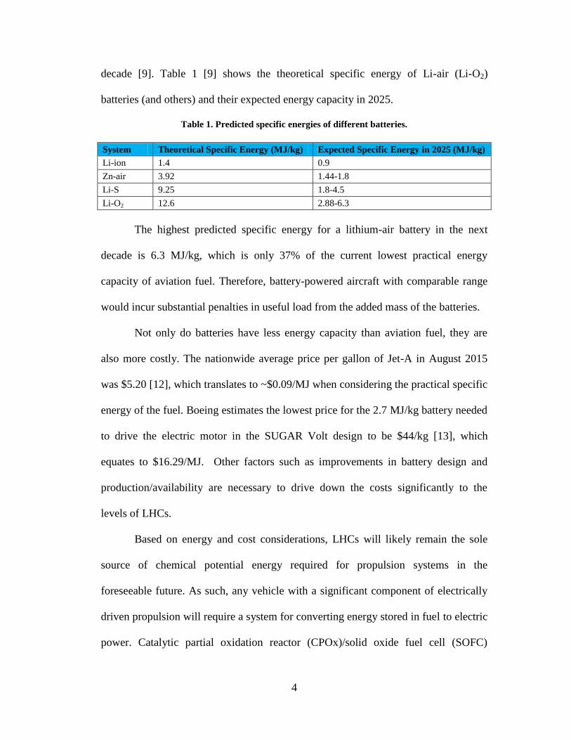
decade [9]. Table 1 [9] shows the theoretical specific energy of Li-air (Li-O2)
batteries (and others) and their expected energy capacity in 2025.
Table 1. Predicted specific energies of different batteries.
System Theoretical Specific Energy (MJ/kg) Expected Specific Energy in 2025 (MJ/kg)
Li-ion 1.4 0.9
Zn-air 3.92 1.44-1.8
Li-S 9.25 1.8-4.5
Li-O2 12.6 2.88-6.3
The highest predicted specific energy for a lithium-air battery in the next
decade is 6.3 MJ/kg, which is only 37% of the current lowest practical energy
capacity of aviation fuel. Therefore, battery-powered aircraft with comparable range
would incur substantial penalties in useful load from the added mass of the batteries.
Not only do batteries have less energy capacity than aviation fuel, they are
also more costly. The nationwide average price per gallon of Jet-A in August 2015
was $5.20 [12], which translates to ~$0.09/MJ when considering the practical specific
energy of the fuel. Boeing estimates the lowest price for the 2.7 MJ/kg battery needed
to drive the electric motor in the SUGAR Volt design to be $44/kg [13], which
equates to $16.29/MJ. Other factors such as improvements in battery design and
production/availability are necessary to drive down the costs significantly to the
levels of LHCs.
Based on energy and cost considerations, LHCs will likely remain the sole
source of chemical potential energy required for propulsion systems in the
foreseeable future. As such, any vehicle with a significant component of electrically
driven propulsion will require a system for converting energy stored in fuel to electric
power. Catalytic partial oxidation reactor (CPOx)/solid oxide fuel cell (SOFC)
5
systems offer a promising method of energy conversion because they can operate on
reformates from LHCs such as aviation fuel and are much more tolerant of carbon
and sulfur compounds present in such fuels.
1.1.3 Fuel Consumption
The ‘relative’ fuel mass flow rate [1] is one way to quantify the effect of
electric power generation on vehicle performance. The relative fuel flow rate is
defined as the ratio of a vehicle’s fuel flow rate at cruise to the fuel flow rate at cruise
when no electrical power is being delivered. Thus, it is a number greater than one that
increases with increasing electric power demand. Waters derived a closed-form
expression for the relative fuel flow rate based on thrust specific fuel consumption of
the propulsive engine ( ), specific energy of the fuel ( ), efficiency of the
electrical conversion system ( ), mass of the electrical generation components
( ), cruise speed ( ), electric power fraction ( ), gravitational acceleration ( ), a
characteristic surface area ( ), and the vehicle’s drag polar ( , , ) [1]:
(2)
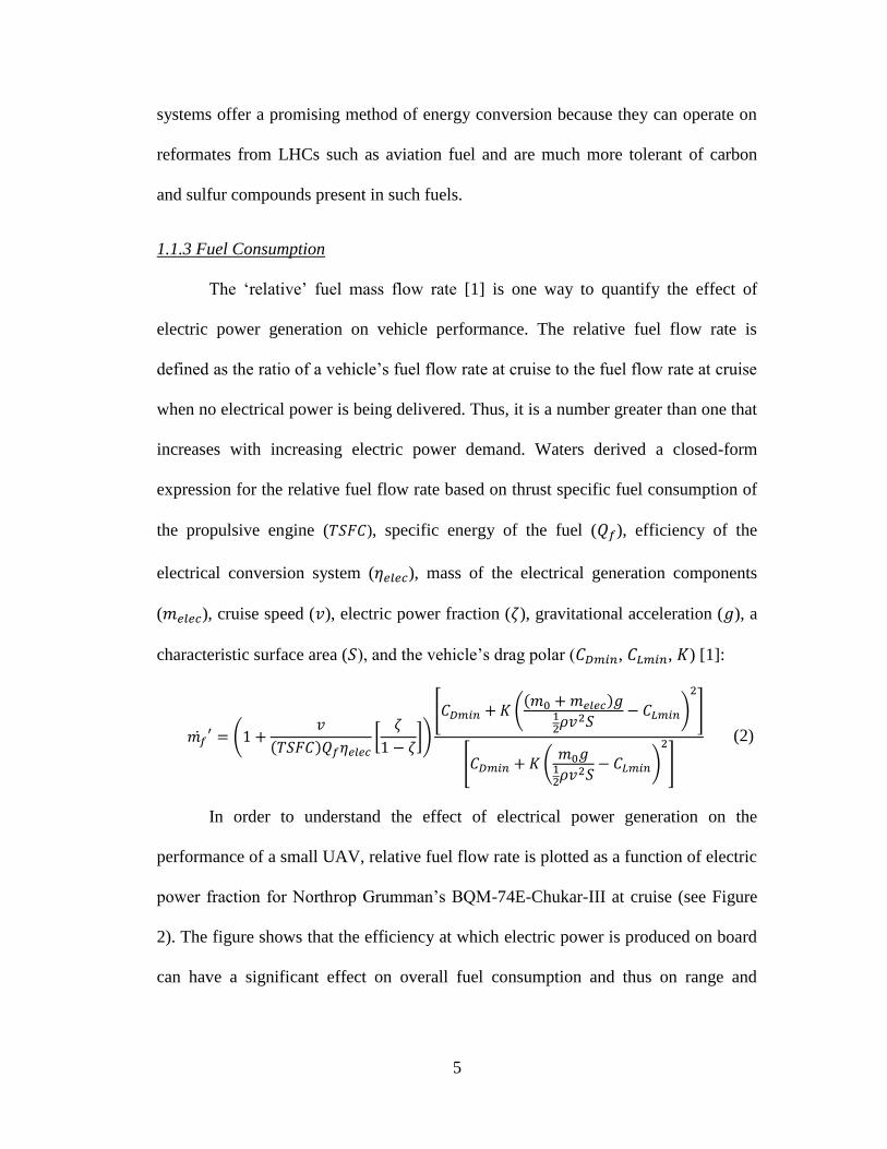
In order to understand the effect of electrical power generation on the
performance of a small UAV, relative fuel flow rate is plotted as a function of electric
power fraction for Northrop Grumman’s BQM-74E-Chukar-III at cruise (see Figure
2). The figure shows that the efficiency at which electric power is produced on board
can have a significant effect on overall fuel consumption and thus on range and

6
endurance. Flight conditions and aircraft specifications [14] used to generate the plots
in Figure 2 are summarized in Table 2.
Table 2. Flight conditions and aircraft specifications for preliminary relative fuel flow rate
calculations.
Flight Conditions
Mach ( ) 0.5
Altitude 40 kft
0.301 kg/m3
147.5 m/s
Aircraft Specifications
33.99 g⁄kN/sec
44 MJ/kg
0.4
0.6
0.697 m2
206.4 kg
Total rated thrust 1068 N
Figure 2. (Top) Relative fuel flow rate vs. electric power fraction; (Bottom) Fuel flow rate
reduction vs. electric power fraction.

7
The top plot in Figure 2 shows that a fuel cell based system consumes less
fuel than a mechanical generator based system because of the higher electrical
conversion efficiency of the fuel cell. The bottom plot of Figure 2 shows that fuel
savings increase with electric power fraction. There is about a 5% and 7% reduction
in fuel flow rate from a generator system for electric power fractions of and
, respectively. For this highly simplified analysis, the electrical system mass
and any coupling effects between the engine and fuel cell are neglected.
Since this thesis involves turbine/fuel cell hybrids, it is useful to briefly
review the operating principles of turbojet engines and fuel cells.
1.2 Turbojets
1.2.1 Fundamentals of Turbojet Operation
Turbojets are a class of gas turbines that utilize the Brayton thermodynamic
cycle to produce thrust. In a turbojet, air enters the inlet and is compressed using
centrifugal or axial turbomachinery called a compressor. After exiting the
compressor, air enters the combustor/burner where energy in the form of heat is
added to the flow due to combustion. Following combustion, air is expanded through
a turbine that drives the compressor. The air exiting the turbine is accelerated through
a nozzle to produce thrust. An after-burner stage may also be present between the
turbine and nozzle where additional fuel is injected and burned to increase the energy
of the flow. The engine considered in this work does not have an after-burner stage.
Figure 3 is a schematic illustration of a turbojet with ‘standard’ stage numbering [10].

8
Figure 3. Schematic of a turbojet engine [10].
The simplest representation of the turbojet’s thermodynamics is the ideal
Brayton cycle in which the working fluid (air in the case of aircraft engines) is
subjected to four processes [15]: isentropic compression, isobaric heat addition,
isentropic expansion, and isobaric heat rejection. These processes are illustrated using
pressure-volume and temperature-entropy diagrams in Figure 4 [16]. It is assumed
here that there is no after-burner stage so the nozzle exit is indicated by stage 6 (and
not stage 7). All processes in the ideal turbojet cycle are assumed to be reversible.
Figure 4. P-v and T-s diagrams of the ideal Brayton cycle.
The net work per unit mass of the ideal Brayton cycle is expressed as a
function of temperatures at each stage in the thermodynamic cycle for constant
[17]:

9
(3)
In Eq. (3), is the ambient temperature and the assumption of isentropic flow
constrains the values of and . This means that maximizing maximizes the
net work of the ideal cycle [15]. However, cannot be increased indefinitely as it is
generally limited by material properties of the turbine inlet.
The thermal efficiency of the ideal turbojet cycle is defined as the ratio of
the net work to heat addition in the burner. Following the relationship for specific
work in Eq. (3), the thermal efficiency can be expressed in terms of temperatures for
a calorically perfect gas [17]:
(4)
The combustion and heat rejection processes are assumed to be isobaric. The other
two processes are assumed to be isentropic [15] so:
(5)
Therefore, , and the expression for thermal efficiency of the Brayton
cycle can be rewritten as a function of ambient temperature and the compressor exit
temperature:
(6)
Using isentropic relations, Eq. (6) can be written in terms of the engine’s compression
ratio:
(7)

10
This expression shows that higher compression ratios lead to higher cycle
efficiencies. For fixed ambient and burner exit temperatures, there is also an optimum
compression ratio that maximizes the net work of the cycle [15]:
(8)
A real turbojet engine is not a closed cycle as described above for the ideal
Brayton cycle, but rather an open cycle where the working fluid (air) is expelled after
the expansion process instead of performing the isobaric heat rejection. While none of
the engine’s components are actually reversible, they are assumed to be adiabatic in
this idealized analysis. Also, fluid velocities in the engine are not negligible
(necessary for flame stabilization in the combustor), and the turbine and compressor
flow rates are not equal because of the potential bleed flows for cooling and the
addition of fuel during combustion [10].
An adiabatic efficiency for the compression process in a real turbojet can be
defined as the ratio of work required in an isentropic process to that required in the
real process [10]:
(9)
Similarly, the adiabatic efficiency of the expansion process in the turbine is defined as
[10]:
(10)
Burner efficiency can be defined as well, which is the fraction of chemical energy
stored in fuel that is released during combustion [10]. This efficiency is generally
close to unity, as there is usually complete combustion of the fuel. Other engine
11
components such as the inlet/diffuser and nozzle introduce losses, but they are
typically small and have little effect on overall performance.
1.2.2 Applications of Small Turbojet Engines
In recent years, small-scale turbojet engines have become attractive propulsive
platforms for small manned aircraft, UAVs, and for research applications where
larger turbojets are not easily accessible.
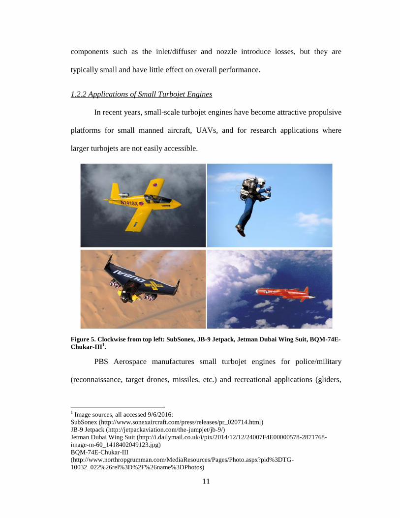
Figure 5. Clockwise from top left: SubSonex, JB-9 Jetpack, Jetman Dubai Wing Suit, BQM-74E-
Chukar-III1.
PBS Aerospace manufactures small turbojet engines for police/military
(reconnaissance, target drones, missiles, etc.) and recreational applications (gliders,
1 Image sources, all accessed 9/6/2016:
SubSonex (http://www.sonexaircraft.com/press/releases/pr_020714.html)
JB-9 Jetpack (http://jetpackaviation.com/the-jumpjet/jb-9/)
Jetman Dubai Wing Suit (http://i.dailymail.co.uk/i/pix/2014/12/12/24007F4E00000578-2871768-
image-m-60_1418402049123.jpg)
BQM-74E-Chukar-III
(http://www.northropgrumman.com/MediaResources/Pages/Photo.aspx?pid%3DTG-
10032_022%26rel%3D%2F%26name%3DPhotos)

12
light sport and experimental aircraft, etc.) [18]. PBS Aerospace’s TJ100 turbojet
engine (1300 N thrust) [19] is currently employed on Sonex’s SubSonex sport aircraft
[20]. The TJ100 has also been refined and optimized for use in reconnaissance UAVs
and target drones [19]. Smaller turbojet engines manufactured by PBS Aerospace
such as the TJ40 (395 N thrust) and the TJ20 (210 N thrust) are more suited for target
and decoy drones [18]. Other small turbojet manufacturers such as AMT Netherlands,
JetCat, and Jet Central produce engines of comparable size and applications. Two of
AMT Netherlands’ Nike engines (784 N thrust) power JetPack Aviation’s JB-9
jetpack [21]. This work uses AMT Netherlands’ Olympus HP (230 N thrust). Jetman
Dubai’s jet-propelled wing suit is powered by four of JetCat’s P400 turbojet engines
(391 N thrust) [22]. Northrop Grumman’s BQM-74E-Chukar-III is a turbojet-
powered aerial target drone that simulates enemy tactical cruise missiles or fighter
aircraft and is heavily employed by the U.S. Navy [14]. Its powerplant is a single
Williams J400-WR-404 turbojet with a maximum thrust of 1068 N.
Because large-scale turbojets are often too complex and expensive to operate
in a laboratory setting, many research universities and institutions employ smaller
turbojets for this purpose. Benini and Giacometti [23] describe the development of a
200 N static-thrust engine at the University of Padova designed specifically for
educational and research activities. The development of small-scale turbojet engines
for research purposes has been investigated by others as well [24], [25]. Industry has
also developed small turbojet engines specialized for lab-scale testing, such as the
SR-30 turbojet produced by Turbine Technologies [26]. Badami et al. [27] perform an
experimental and numerical analysis of the thermodynamic cycle of the SR-30 for use

13
in later studies of examining the use of alternative fuels in gas turbine engines. AMT
Netherlands offers modifications to their existing gas turbine models for static testing.
This work uses AMT’s Olympus HP turbojet in “University Configuration”, meaning
the engine comes equipped with stagnation temperature and pressure measurement
ports at each axial stage along the engine [28]. AMT engines in “University
Configuration” also come with an analog throttle controller for ground testing. The
AMT Olympus HP is a popular turbojet model at other universities as well [29]–[35].
1.3 Fuel Cells
1.3.1 Fundamentals of Fuel Cell Operation
Combustion engines convert chemical potential energy stored in a fuel stream
into thermal power, the thermal power into mechanical power, and then the
mechanical power into electrical power via a mechanical generator. Fuel cells convert
chemical energy in a fuel stream directly to electrical power. While this single-step
electrical conversion process is usually much more efficient than the multi-step
process associated with engines, the fuel cell requires other ‘balance of plant’
components like pumps, blowers, controls, etc. whose losses significantly degrade the
overall performance of the energy conversion system.

14
Figure 6. Schematic of a solid oxide fuel cell [1].
A schematic illustration of a solid oxide fuel cell is shown in Figure 6 [1]. A
hydrogen ion (or proton) carrier such as hydrogen or carbon monoxide gas enters the
anode side of the fuel cell and an oxidizer such as oxygen or air enters the cathode
side. Oxidation and reduction reactions occur at the anode and cathode. O2-
ions are
transported from the cathode across a solid ceramic electrolyte to the anode, where
oxidation occurs. This is in contrast to a PEM fuel cell, where H+ ions (protons) are
transported across the electrolyte. Electrons cannot flow through the electrolyte, so
instead they flow from the anode to the cathode through a load to produce electrical
power. Other types of fuel cells will be discussed shortly.
The following reaction occurs at the anode [36]:
(11)
The electrons produced in this oxidation reaction flow through the external load on
their way back to the cathode where they complete the reaction. The reduction
reaction that occurs at the cathode is given by [36]:

15
(12)
The O2-
ions produced at the cathode diffuse across the electrolyte to complete the
oxidation reaction in the anode. Thus, it is essential that the electrolytic membrane
has physical properties that allow the transport of O2-
ions without conducting
electrons. The total electrical power produced by the fuel cell is the product of the
current and electric potential across the fuel cell.
The variation of fuel cell voltage with pressure is given by [36]:
(13)
where is the number of electrons in the reaction. Eq. (13) shows that the change in
reversible fuel cell voltage with pressure is related to the change in specific volume of
the reaction. If there is a negative change in reaction volume (i.e., less moles of
product than reactants), the cell voltage will increase with increasing pressure
according to Le Chatelier’s principle [16]. Assuming the ideal gas law is applicable,
Eq. (13) can be written as [36]:
(14)
Similar to Eq. (13), for reactions with the reversible cell voltage will increase
with increasing pressure. Equations (13) and (14) show that increasing the operating
pressure enables a fuel cell to produce more power with the same current density.
This means the higher pressure system operates at a higher voltage and more
efficiently. While there are diminishing returns because the derivative in Eq. (14) is
inversely proportional to pressure, it suggests that placing the fuel cell in parallel with
the combustor and thus at elevated pressure should improve performance.

16
The cycle efficiencies of engines and fuel cells have different temperature
dependences. The maximum theoretical efficiency of any heat engine is the Carnot
efficiency [37]:
(15)
In Eq. (15), and are the temperatures of the low and high temperature reservoirs
in the heat engine cycle. The Carnot efficiency is the maximum efficiency allowed by
the second law of thermodynamics. However, a Carnot efficiency of unity is
physically impossible because this would require the low reservoir temperature to be
absolute zero or an infinitely high reservoir temperature.
The maximum theoretical efficiency achieved by any fuel cell is given by
[37]:
(16)
where is the change in sensible enthalpy and is the change in Gibbs free
energy. The change in Gibbs free energy decreases with increasing temperature in
any real process with an entropy change. Thus, a fuel cell’s efficiency decreases with
increasing operating temperature whereas a heat engine’s increases. This is illustrated
in Figure 7 [1].

17
Figure 7. Efficiencies of ideal heat engine and fuel cell vs. temperature [1].
The Carnot efficiency curve in Figure 7 assumes that , and the
fuel cell curve was generated for a fuel cell operating at 1 atm, where the oxidizer is
air and the fuel is composed of 80% hydrogen and 20% water vapor [1]. Figure 7
shows that fuel cell efficiency is greatest at low temperatures, whereas heat engine
efficiency is greatest at high temperatures. The efficiencies in Figure 7 depict the
maximum theoretical efficiencies. These efficiencies are not attainable in real
systems, so comparisons between heat engines and fuel cells must be made based on
practical performance of these systems.
There are five major types of fuel cells which are mainly differentiated by
their electrolytes [36]:
1. Phosphoric acid fuel cell (PAFC)
2. Polymer electrolyte membrane fuel cell (PEMFC)
3. Alkaline fuel cell (AFC)
4. Molten carbonate fuel cell (MCFC)
5. Solid oxide fuel cell (SOFC)
18
PAFCs use liquid H3PO4 (phosphoric acid) contained in a SiC matrix between
porous electrodes coated with a platinum catalyst to form the electrolyte [36].
PEMFCs employ a polymer electrolyte membrane that conducts protons [36]. AFCs
are constructed from a liquid potassium hydroxide electrolyte where OH- ions diffuse
from the cathode to the anode [36]. The electrolyte in MCFCs is a molten mixture of
alkali carbonates (Li2CO3 and K2CO3) in a matrix of LiOAlO2, where the carbonate
ion CO32-
is the charge carrier [36]. SOFCs generally contain ceramic electrolytes
such as yttria stabilized zirconia (YSZ) that conduct oxygen ions [36]. For SOFCs,
the diffusion of oxygen ions across the YSZ electrolyte membrane is most effective at
high fuel cell operating temperatures. For example, the conductivity of YSZ at 800°C
is about 0.02 S/cm and increases to 0.1 S/cm at 1000°C [37]. Therefore, SOFCs
require high operating temperatures and a thin YSZ membrane. Advantages of a high
operating temperature include fuel flexibility and the ability to utilize a cogeneration
scheme with the wasted heat generated from the fuel cell.
The anode electrode in SOFCs must be able to withstand the highly reducing
environment of the fuel-side reaction and high operating temperatures of the fuel cell.
The most common choice for anode material is a nickel-YSZ cermet – a mixture of
ceramic and metal [36]. Nickel provides effective electron conductivity and serves as
an effective reaction catalyst. The YSZ provides porosity and mechanical stability to
the anode and has resilient thermal properties. Similarly, the cathode electrode must
have sufficient porosity to allow the diffusion of reactants and serve as an effective
electron conductor. The cathode material must also be well-suited for the highly
oxidizing air/oxidizer-side reaction and of course the high fuel cell temperatures.

19
Common electrode cathode materials for SOFCs are strontium-doped lanthanum
manganite, lanthanum-strontium ferrite, lanthanum-strontium cobaltite, and
lanthanum strontium cobaltite ferrite [36]. These materials exhibit sufficient diffusive
and conductive properties, and offer high catalytic activity for the cathode reaction.
As stated above, one of the advantages of SOFCs is their carbon tolerance
(due to their high operating temperature) which enables them to operate on syngas
(mixtures of H2, CO, and CO2) and other hydrocarbon reformates. While this enables
SOFCs to consume energy dense fuels like liquid hydrocarbons (LHCs), a separate
reformer such as a catalytic partial oxidation reactor (CPOx) is usually required.
However, this adds complexity and balance of plant components to the fuel cell
system that reduce overall system efficiency. Other advantages of SOFCs include the
use of non-precious metal catalysts (which reduces cost) and their relatively high
power density which is essential for aerospace applications where lower mass
components are preferred.
Despite the benefits offered by SOFCs, they have several shortcomings. High
operating temperatures present issues with thermal management. They also require
the use of fragile ceramic materials in the membrane-electrode assembly that are
prone to fracturing. Thus, it is important to minimize thermal gradients and manage
cyclic heating and cooling carefully. Sealing is also a challenge as most sealants
cannot withstand the high temperatures. In spite of the high operating temperatures,
contamination and poisoning remain significant problems because syngas from
aerospace fuels can contain high levels of sulfur that has been shown to inhibit the Ni
catalyst activity in the anode [38]. Thus, the ‘fuel processor’ may have to contain

20
other components besides a reformer and this drives up the size of the system and the
balance of plant losses associated with its operation. For example, a fuel cell stack
from Ballard Power Systems weighs 0.8-9 kg per kW of electrical output, but the full
system weighs roughly 15-110 kg per kW [39]. The balance of plant components can
also be significantly more expensive than the fuel cell stack [40].
SOFCs commonly use catalytic partial oxidation (CPOx) reactors as fuel
reformers. A CPOx is typically made with porous alumina foams coated in a catalyst
[41]–[43]. Such foams are ceramic and achieve porosities of 80-90%, resulting in
minimal pressure losses [44]. Catalysts for the foams can be made from platinum [42]
or rhodium [38], [43]. At high operating temperatures, well designed CPOx reformers
can operate close to chemical equilibrium [38].
CPOx reactors operate fuel rich (with less than stoichiometric oxygen (O2)
concentrations) to partially combust (or oxidize) the fuel into hydrogen (H2) and
carbon monoxide (CO). The partial oxidation of propane is shown in Eq. (17) and can
be compared to the complete (stoichiometric) oxidation of propane with O2 in Eq.
(18).
(17)
(18)
For any hydrocarbon fuel, partial oxidation is defined as:
(19)
In Eq. (19), is the number of carbon atoms and is the number of hydrogen atoms.

21
1.3.2 Applications of Fuel Cells in Aircraft
Fuel cell technology has already been incorporated onto aircraft as the sole
powerplant for propulsion. This is in contrast to the current work that aims to advance
the development of a hybrid GT/SOFC system for combined propulsion and electric
power generation.
Figure 8. Clockwise from top left: Ion Tiger, Intelligent Energy’s Quadrotor Prototype, Boeing’s
Experimental FC Aircraft2.
The U.S. Naval Research Laboratory’s Ion Tiger UAV employs a 550 W
hydrogen fuel cell as its propulsion system and can carry a 5 lbf (22.2 N) payload
[45]. Recent development of a cryogenic fuel storage tank and delivery system for
liquid hydrogen fuel allowed the Ion Tiger to successfully complete a 48-hour long
flight [46]. Intelligent Energy has recently developed a small quadrotor prototype
powered by a hybrid hydrogen fuel cell/battery system and has been able to extend
2 Image sources, all accessed 9/7/2016:
Ion Tiger (http://www.naval-technology.com/projects/ion-tiger-uav/)
Intelligent Energy’s Quadrotor Prototype (http://www.intelligent-energy.com/news-and-
events/company-news/2015/12/15/intelligent-energy-hydrogen-fuel-cells-significantly-extend-drone-
flight-time/)
Boeing’s Experimental FC Aircraft (http://www.popularmechanics.com/flight/a2761/4257294/)
22
the UAV’s endurance by several hours [47]. The successful demonstration of their
quadrotor drone in early 2016 has led to collaboration with a major drone
manufacturer [48]. Boeing has successfully flown a small manned aircraft powered
by a hybrid PEM fuel cell/lithium ion battery propulsion system [49]. The airframe
for Boeing’s experimental aircraft was a two-seat Dimona motor-glider. Despite the
success of this small fuel cell-powered aircraft, Boeing researchers do not believe fuel
cells will ever provide primary power for larger commercial aircraft [49]. This
sentiment validates the need for investigating hybrid technology such as GT/SOFC
systems to power aircraft with larger payload requirements.
1.4 Gas Turbine/Solid Oxide Fuel Cell Hybridization
1.4.1 Advantages of System Coupling
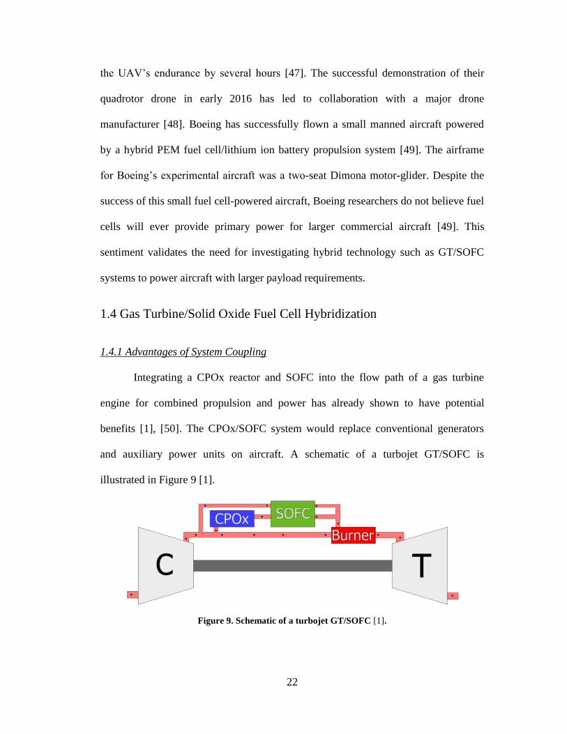
Integrating a CPOx reactor and SOFC into the flow path of a gas turbine
engine for combined propulsion and power has already shown to have potential
benefits [1], [50]. The CPOx/SOFC system would replace conventional generators
and auxiliary power units on aircraft. A schematic of a turbojet GT/SOFC is
illustrated in Figure 9 [1].
Figure 9. Schematic of a turbojet GT/SOFC [1].

23
In the proposed GT/SOFC system, bleed air exiting the compressor is supplied
to the CPOx/SOFC system. The bleed air provides cooling for the system and
oxidizer for the cathode of the fuel cell. Although not indicated in Figure 9, the CPOx
also receives its own fuel supply. Unused fuel and products from the CPOx/SOFC
reaction are fed back into the burner of the turbojet to be recovered in the Brayton
cycle. A hypothetical layout of a turbojet GT/SOFC with the SOFC in an annular duct
around the engine is depicted in Figure 10 [1].
Figure 10. Engine layout of turbojet GT/SOFC [1].
The coupled behavior between the gas turbine and SOFC present several
advantages for the hybrid system. Many fuel cell balance of plant functions are
absorbed by the gas turbine. For example, the fuel cell does not need separate pumps
or blowers because the gas turbine supplies air to the system. Air provided by the gas
turbine is pressurized from the compressor stage, improving fuel cell efficiency and
power density. The pressurized air is also heated, further improving fuel cell
conversion and making it easier to maintain the membrane electrode assembly at the
proper temperature. Unreacted fuel and waste heat generated by the CPOx/SOFC
system is recovered in the Brayton cycle when products from the reaction flow into
CPOxSOFC
Supply/Cooling air

24
the burner. In addition, the faster transient response of the Brayton cycle could
improve the transient response of the fuel cell.
1.4.2 Challenges
Pressure losses associated with the CPOx/SOFC system could have
detrimental effects on overall performance of the gas turbine. Although the porous
alumina foam catalyst in the CPOx has relatively low pressure drop compared to
other catalysts [44], the losses can still be significant. Pressure losses due to friction
will also occur in the flow channels of the SOFC. Additional pressure losses will arise
from bleeding air from the compressor stage of the GT and reintroducing the flow
back into the burner. When designing the physical hybrid system, it is essential that
the pressure drop across the CPOx/SOFC is no greater than the pressure drop incurred
in the GT combustor. If the CPOx/SOFC pressure drop is greater than that across
burner, air will not flow into CPOx/SOFC assembly or the gas turbine will encounter
further losses in the Brayton cycle. Physical integration of the fuel cell exhaust paths
with the burner is another challenge facing the design of a hybrid system.
Modifications to the burner will likely add mass to the system, and altering the flow
path could result in combustion instability. The effect of introducing low molecular
weight fuel species such as H2 and CO into the combustion process could also be
unpredictable. Furthermore, injecting SOFC exhaust upstream of the turbine stage of
the gas turbine could result in severe complications. If ceramic materials in the SOFC
were to fracture due to excessive heating or impact, the debris could enter the
combustor and turbine. This debris would cause damage to the turbine blades and
reduce turbine efficiency or at worst cause catastrophic engine failure.

25
1.4.3 Literature Review of GT/SOFC Systems
A summary of the literature investigating hybrid GT/SOFC systems is
presented in Table 3 [1]. Most of the work on engine-integrated SOFCs has been
focused primarily on stationary power generation in terrestrial applications. Research
on GT/SOFC systems for airborne applications is typically focused on replacing
existing APUs with FC technology. These APU applications are strictly for electrical
power generation and are separate from the main propulsion of the aircraft. Only a
few studies have investigated hybrid GT/SOFC systems for combined propulsion and
electrical power generation.
Recent studies conducted at the University of Maryland [1], [50] have further
explored the potential benefits of a GT/SOFC system for combined propulsion and
power on aircraft. Waters and Cadou develop Numerical Propulsion System
Simulation (NPSS) thermodynamic models of SOFCs, CPOx reactors, and multiple
GT engine types [1], [50]. The models account for realistic equilibrium gas phase and
electrochemical reactions, pressure losses, and heat losses. It is shown that hybrid
systems can reduce fuel consumption by 3-4% for a 50 kW SOFC system integrated
with a 35 kN rated engine. Larger reductions of 15-20% are predicted for 200 kW
systems. Waters and Cadou also show that GT/SOFC systems can produce more
electric power than mechanical generator-based systems before reaching turbine inlet
temperature limits. Finally, Waters and Cadou examine the aerodynamic drag effects
of engine-airframe integration of the SOFC assembly. Ultimately, the studies
performed by Waters and Cadou show that integrated GT/SOFC systems for
combined propulsion and power exhibit better overall performance than powerplants

26
with separate components. Although hybrid GT/SOFC systems appear to offer better
performance than mechanical generator- or APU-based systems, it appears no studies
to date have proposed constructing a physical prototype.

27
Table 3. Summary of GT/SOFC literature [1].
Authors Platform Size Reformer/FC Fuel FC model GT model Efficiency Notes Ground-based:
Calise et. al. [51] MATLAB 1.5 MW IR-SOFC Natural
Gas Validated vs. data Performance maps
ηelec=68%,
ηsys>90% Cost optimization
Haseli et. al. [52] MATLAB 2.4 MW IR-SOFC Methane Zero-D Constant efficiencies ηsys=60% Focus on irreversibilities
Abbasi & Jang [53] 132 kW IR-SOFC Zero-D Constant efficiencies Power conditioning; transient response
Chan et. al. [54] 2.1 MW IR-SOFC Natural Gas
Zero-D, validated vs. data
Constant efficiencies ηelec=62%, ηsys=84%
Palsson et. al. [55] Aspen Plus 500 kW pre-reformer,
SOFC Methane
2-D, validated vs.
literature
Aspen Plus std.
models
ηelec=60%,
ηsys=86% Combined power and heat prod.
Costamaga et. al. [56] MATLAB 300 kW steam ref., SOFC Natural Gas
Zero-D Performance maps ηsys>60% On and off-design analysis
Lim et. al. [57] Experiment 5 kW pre-reformer,
SOFC
Natural
Gas Working on GT-SOFC
Suther et. al. [58] Aspen Plus steam ref., SOFC Syngas Zero-D Aspen Plus std.
models
Zhao et. al. [59] Coal
syngas Zero-D Ideal GT ηsys=50-60%
Leto et. al. [60] IPSE Pro 140 kW IR molten
carbonate
Natural
Gas Zero-D IPSE Pro std. models ηsys=60-70%
Veyo et. al. [61] 300 kW,
1MW
Natural
Gas ηsys=59%
APUs:
Freeh et. al. [62] NPSS 200 kW steam ref., SOFC Jet-A Zero-D, validated vs. data
Performance maps ηelec=65%, ηsys=40%
Steffen et. al. [63] NPSS 440 kW,
1396 kg steam ref., SOFC Jet-A Zero-D Performance maps ηsys=62%
Freeh et. al. [64] NPSS 440 kW steam ref., SOFC Jet-A Zero-D Performance maps ηsys=73% On and off-design analysis
Eelman et. al. [65] MATLAB 370 kW steam ref., PEM + SOFC
Jet fuel SOFC: ηsys>70%, PEM: ηsys>35%
Aircraft integration approaches
Rajashekara et. al. [66] 440 kW,
>880 kg steam ref., SOFC Jet fuel Zero-D
SL: ηsys=61%,
Cruise: ηsys=74%
Braun et. al. [67] UTRC prop. 300 kW autothermal ref., SOFC
Jet-A SL: ηsys=53%, Cruise: ηsys=70%
All-Electric:
Himansu et. al. [68] MATLAB 20 kW, 50kW
SOFC H2 Zero-D Constant efficiencies
Aguiar et. al. [69] 140 kW SOFC H2 Constant efficiencies Single: ηsys=54%,
Multi: ηsys=66%
Multiple stacks: fuel in parallel, air in
series
Bradley & Droney [70] Spreadsheet SOFC H2 Zero-D
Bradley & Droney [71] GE prop. SOFC LNG SFC ~0.125 lb/lbf/hr

28
1.5 Objectives
The overall objective of this research program is to take initial steps toward
constructing a bench-scale prototype of a hybrid GT/SOFC so that the challenges
associated with building a practical, flight-ready system may be identified. The first
step is to develop experimentally validated thermodynamic models of the gas turbine
and SOFC as separate components. The separate models will be combined to develop
a model of the hybrid GT/SOFC system that, in turn, can be used to design the bench-
scale prototype.
The foci of this thesis are the development and experimental validation of a
thermodynamic model for a small gas turbine engine suitable for building a bench-
scale GT/SOFC hybrid.
1.6 Previous Work
Since this thesis focuses on the development of an experimentally validated
model of a small GT needed to construct a bench-scale GT/SOFC system, an
investigation of previous testing and modeling of small gas turbines is also necessary.
Numerous studies have already investigated performance of the AMT Olympus
turbojet engine considered in this work [29]–[35]. Horoufi and Boroomand [32],
Grzeszczyk et. al. [31], and Laskaridis et. al. [33] focus on the development of a test
facility and performance of the AMT Olympus. Horoufi and Boroomand develop an
outdoor test bed that measures RPM, thrust, fuel flow rate, compressor exit
temperature, and exhaust gas total temperature [32]. As is done in this work, Horoufi
and Boroomand calibrate their thrust stand using a cable/pulley system and measure
fuel flow gravimetrically [32]. Grzeszczyk et. al. measure thrust, fuel flow rate, RPM,

29
and all axial stage temperatures/pressures measured in this work (discussed later), but
they do not measure air flow rate (as is done in this work). Grzeszczyk et. al. measure
fuel flow volumetrically using a flow meter, and they also measure engine vibration
[31]. Laskaridis et. al. use CFD to optimize the aerodynamic performance of an
enclosed (indoor) test cell that imitates full-scale test cells for larger turbojet engines
[33]. Laskaridis et. al. focus more on design of the test facility instead of measuring
performance of the Olympus.
References [29], [30], [34], [35] focus on both experimental and numerical
analysis of the Olympus. Al-Alshaikh measures thrust, RPM, fuel flow rate, air mass
flow rate, flow velocities inside the test cell, pressure distribution inside the test cell,
and temperatures at the inlet/exit of the test cell, engine, and detuner [29]. Al-
Alshaikh uses the CFD package Fluent to predict performance of the Olympus [29].
Bakalis and Stamatis measure compressor exit total/static pressure and total
temperature, turbine inlet total temperature and pressure, turbine exit total/static
pressure and total temperature, RPM, fuel flow rate, and thrust [30]. As in this work,
Bakalis and Stamatis use scaled compressor and turbine performance maps for off-
design performance estimation. They experienced difficulty matching the measured
and model-predicted TIT (as was the case in this work too). However, they found that
recalibrating their model based on static pressure instead of total pressure
measurements at the turbine produced more reasonable predictions. Leylek measures
thrust, air flow rate, fuel flow rate, RPM, and the internal stage temperatures and
pressures [34]. Leylek models the engine’s thermodynamic cycle using a combination
of methods that include: the commercially available Gasturb code and a python script

30
for overall performance simulation, CFD (Fluent and Numeca), Meanline and
ThroughFlow empirical tools, and map scaling for turbomachinery performance, and
empirical loss models for the combustor and ducts/nozzle performance [34]. Rahman
and Whidborne use measured fuel flow, thrust, compressor pressure ratio, air flow,
RPM, and exhaust gas temperature for the Olympus to examine the effect of engine
bleed on steady state and transient performance of the engine using
MATLAB/Simulink as the modeling tool [35]. They also use representative
turbomachinery performance maps for the Olympus in their model.
1.7 Approach
The approach taken to achieve the goals of this thesis is outlined below:
Identify a commercially available small gas turbine engine suitable for indoor
bench-scale testing in the facilities at the University of Maryland (UMD)
Develop a thermodynamic model of the engine using Numerical Propulsion
System Simulation (NPSS)
Design and construct a test facility for safe indoor testing of the engine
Measure the engine’s performance parameters – thrust, air flow rate, fuel
flow rate, and internal stage temperatures and pressures
Use the measured performance data to validate the NPSS model of the engine

31
Chapter 2: Engine Selection
Cost, size, and availability of turbomachinery performance maps were among
the considerations for selecting a suitable gas turbine platform for a bench-scale
GT/SOFC prototype. A complete list of the considerations/requirements used to
identify a gas turbine engine is included below:
Relatively inexpensive
Maximum thrust and air flow rate are suitable for the previously designed
engine exhaust ejector at UMD [72]
Compressor and turbine performance maps are available
Engine can easily be modified for measurements of internal stage
temperatures and pressures and the eventual integration of the fuel cell system
Engine sensor output (RPM, exhaust temperature, etc.) collection is available
Engine controller can easily be configured for static operation
The candidate gas turbine engine platforms are described in Table 4.

32
Table 4. Candidate gas turbine platforms.
Engine P200-SX
Turbine
Complete
Olympus HP
(University
Configuration)
Titan Mammoth
SP Series K-210G
Manufacturer/
Dealer
JetCat USA
[73]
AMT
Netherlands
[21]
AMT
Netherlands
[21]
Jet Central
USA [74]
KingTech
Turbines [75]
Price $5,495.00 $8,979.20 $11,072.20 $4,795.00 $4,350.00
Max Thrust
231 N 230 N (@ STP
and 108,500
RPM)
392 N (@
STP and
96,000 RPM)
225 N 206 N
Weight 25 N 28.5 N 35 N 22 N 16 N
Diameter 12.88 cm 12.95 cm 14.73 cm 12.45 cm 11.25 cm
Length 34.67 cm 37.34 cm 38.35 cm 34.9 cm 28.6 cm
RPM Range 33,000-
112,000
112,000 (max) 100,000 (max) 28,000-
104,000
33,000-
120,000
Max Exhaust
Temp.
750 °C 750 °C 875 °C 750 °C 650 °C
Fuel Rate @
Full Power
0.0117 kg/sec 0.0106 kg/sec
(@ 230 N)
0.017 kg/sec
(@ 392 N)
0.0109 kg/sec 0.0098
kg/sec
Turbine Map
Available
No No
No No -----
Compressor
Map Available
No Yes Yes No -----
Sensors
Turbine temp.
and RPM,
fuel flow
(ml/min)
Tt3, Tt4, Tt5,
Tt6, Ps3,Pt3,
Pt4, Pt5, RPM
RPM, exit
temp., others
upon request
RPM, exit
temp. -----
Sensor Output
Collection
Available
Yes (sold
separately)
Yes (included
with engine)
Yes (included
with engine)
Yes (included
with engine) -----
Electronic
Controller
Available
-Yes
(included
with engine)
-usage notes
in manual
-Yes (included
with engine)
-usage notes in
manual
-analog throttle
available for
static testing
-Yes (included
with engine)
-usage notes
in manual
-analog
throttle
available for
static testing
-Yes
(included
with engine)
-usage notes
in manual -----
**Note: All engine prices listed are accurate as of April 2015.
All candidate engines considered produce a maximum thrust of less than 445
N. This is because the current work uses an exhaust ejector system that was designed
previously at UMD for testing of a gas turbine engine with a maximum thrust of 467
N [72]. The least expensive engines are JetCat’s P200-SX, Jet Central’s Mammoth SP
Series, and KingTech’s K-210G. However, the compressor and turbine performance

33
maps are unavailable for these engines. AMT is willing to provide compressor maps
for the Olympus and Titan, but unfortunately they do not generate performance maps
for their turbines. The availability of turbomachinery maps greatly assists the
modeling effort as producing these maps would require additional experimental data.
AMT also offers analog throttle controllers for static ground operation of their
engines. In addition, AMT offers factory-installed measurement ports (“University
Configuration”) for axial stage stagnation temperatures and pressures. This saves the
time and risk of tampering with the engine’s flow path to make these measurements.
Because AMT is capable of making these modifications to their engines, it is likely
they could eventually assist with the physical integration of a fuel cell system. After
narrowing the engine candidates down to AMT’s Olympus and Titan, it was
ultimately decided that the Olympus is the best choice for a GT/SOFC prototype due
to budget constraints and the availability of other performance data from other
universities [29]–[35]. A picture of AMT’s Olympus in “University Configuration” is
provided in Figure 11.
Figure 11. AMT Olympus in University Configuration.

34
The AMT Olympus is a small turbojet engine that produces a maximum rated
thrust of 230 N and has a maximum rated air flow rate of 0.45 kg/sec. It utilizes a
centrifugal compressor with a maximum compression ratio of = 3.8, annular
combustor, and an axial turbine. The Olympus is a direct electric start engine that
operates on Jet-A fuel. Figure 12 is a cutaway illustration of the Olympus showing its
internal stage components and the locations of the temperature and pressure
measurement ports [28].
Figure 12. Schematic diagram of the Olympus and its measurement port locations.
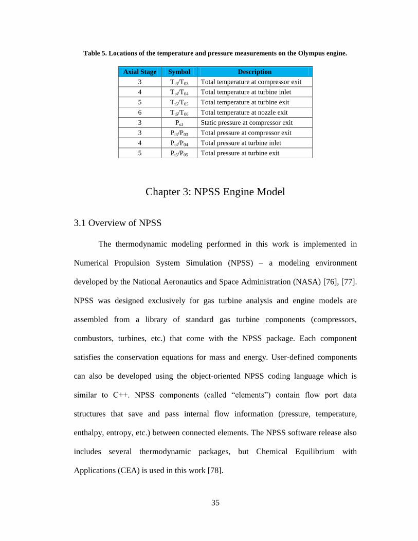
Table 5 shows the locations of the various temperature and pressure
measurements as a function of position (stage) in the cycle:
35
Table 5. Locations of the temperature and pressure measurements on the Olympus engine.
Axial Stage Symbol Description
3 Tt3/T03 Total temperature at compressor exit
4 Tt4/T04 Total temperature at turbine inlet
5 Tt5/T05 Total temperature at turbine exit
6 Tt6/T06 Total temperature at nozzle exit
3 Ps3 Static pressure at compressor exit
3 Pt3/P03 Total pressure at compressor exit
4 Pt4/P04 Total pressure at turbine inlet
5 Pt5/P05 Total pressure at turbine exit
Chapter 3: NPSS Engine Model
3.1 Overview of NPSS
The thermodynamic modeling performed in this work is implemented in
Numerical Propulsion System Simulation (NPSS) – a modeling environment
developed by the National Aeronautics and Space Administration (NASA) [76], [77].
NPSS was designed exclusively for gas turbine analysis and engine models are
assembled from a library of standard gas turbine components (compressors,
combustors, turbines, etc.) that come with the NPSS package. Each component
satisfies the conservation equations for mass and energy. User-defined components
can also be developed using the object-oriented NPSS coding language which is
similar to C++. NPSS components (called “elements”) contain flow port data
structures that save and pass internal flow information (pressure, temperature,
enthalpy, entropy, etc.) between connected elements. The NPSS software release also
includes several thermodynamic packages, but Chemical Equilibrium with
Applications (CEA) is used in this work [78].

36
CEA performs chemical equilibrium calculations to determine a flow’s
thermodynamic state. These calculations are based on the minimization of Gibbs’ free
energy, which produces a solution that is independent of activation energy or reaction
kinetics [78]. Although equilibrium calculations are not usually needed to model non-
emission related aspects of gas turbine performance, they are required in hybrid
GT/SOFC systems because fuel cell models require knowledge of speciation and the
bulk heating value of the fuel cell exhaust varies with operating condition. The need
to incorporate multi-step equilibrium chemistry is one reason why more
computational resources are required to simulate hybrid GT/SOFC systems than
stand-alone gas turbines.
NPSS uses a quasi-Newton’s method solver to find solutions (operating
points) to the set of coupled differential equations that represent the system. The
equations are solved by specifying a set of independent variables (called
‘independents’) and a set of target conditions (‘dependents’) that are defined using
equalities. The solver iteratively adjusts the values of the independents to converge on
a solution that satisfies all the dependent conditions. An example of an independent-
dependent relationship is adjusting the shaft speed (RPM) such that power input to
the compressor equals the power extracted from the turbine. Another example is
varying the air mass flow into the engine such that the calculated thrust matches the
user-specified thrust. A properly configured solver has an equal number of
independents and dependents. A detailed list of the independent variables and
dependent conditions used in this work will be presented later.
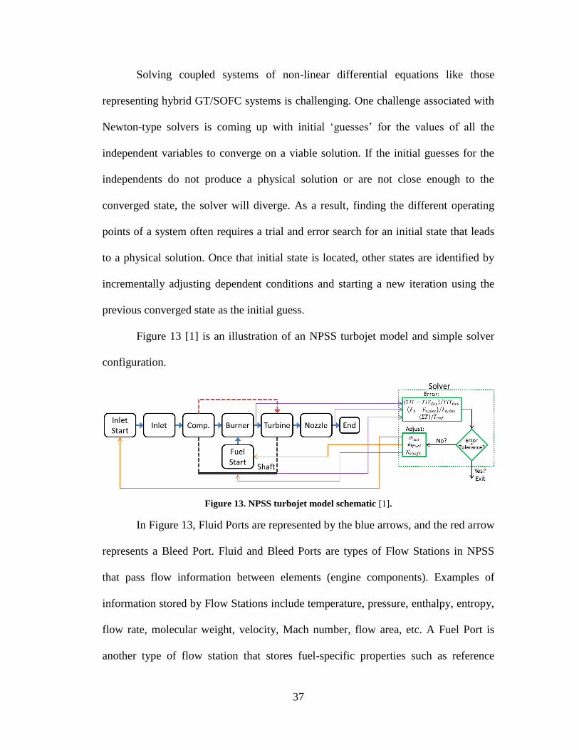
37
Solving coupled systems of non-linear differential equations like those
representing hybrid GT/SOFC systems is challenging. One challenge associated with
Newton-type solvers is coming up with initial ‘guesses’ for the values of all the
independent variables to converge on a viable solution. If the initial guesses for the
independents do not produce a physical solution or are not close enough to the
converged state, the solver will diverge. As a result, finding the different operating
points of a system often requires a trial and error search for an initial state that leads
to a physical solution. Once that initial state is located, other states are identified by
incrementally adjusting dependent conditions and starting a new iteration using the
previous converged state as the initial guess.
Figure 13 [1] is an illustration of an NPSS turbojet model and simple solver
configuration.
Figure 13. NPSS turbojet model schematic [1].
In Figure 13, Fluid Ports are represented by the blue arrows, and the red arrow
represents a Bleed Port. Fluid and Bleed Ports are types of Flow Stations in NPSS
that pass flow information between elements (engine components). Examples of
information stored by Flow Stations include temperature, pressure, enthalpy, entropy,
flow rate, molecular weight, velocity, Mach number, flow area, etc. A Fuel Port is
another type of flow station that stores fuel-specific properties such as reference
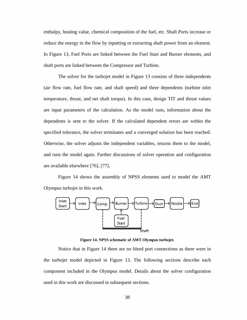
38
enthalpy, heating value, chemical composition of the fuel, etc. Shaft Ports increase or
reduce the energy in the flow by inputting or extracting shaft power from an element.
In Figure 13, Fuel Ports are linked between the Fuel Start and Burner elements, and
shaft ports are linked between the Compressor and Turbine.
The solver for the turbojet model in Figure 13 consists of three independents
(air flow rate, fuel flow rate, and shaft speed) and three dependents (turbine inlet
temperature, thrust, and net shaft torque). In this case, design TIT and thrust values
are input parameters of the calculation. As the model runs, information about the
dependents is sent to the solver. If the calculated dependent errors are within the
specified tolerance, the solver terminates and a converged solution has been reached.
Otherwise, the solver adjusts the independent variables, returns them to the model,
and runs the model again. Further discussions of solver operation and configuration
are available elsewhere [76], [77].
Figure 14 shows the assembly of NPSS elements used to model the AMT
Olympus turbojet in this work.
Figure 14. NPSS schematic of AMT Olympus turbojet.
Notice that in Figure 14 there are no bleed port connections as there were in
the turbojet model depicted in Figure 13. The following sections describe each
component included in the Olympus model. Details about the solver configuration
used in this work are discussed in subsequent sections.
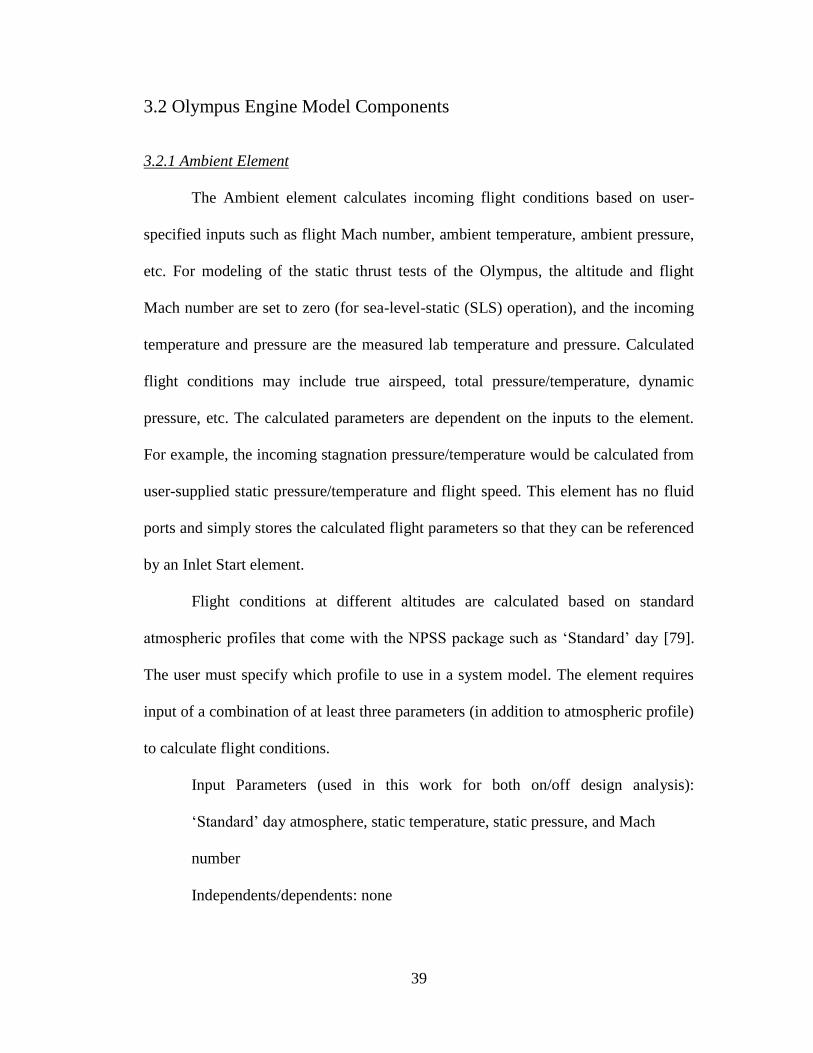
39
3.2 Olympus Engine Model Components
3.2.1 Ambient Element
The Ambient element calculates incoming flight conditions based on user-
specified inputs such as flight Mach number, ambient temperature, ambient pressure,
etc. For modeling of the static thrust tests of the Olympus, the altitude and flight
Mach number are set to zero (for sea-level-static (SLS) operation), and the incoming
temperature and pressure are the measured lab temperature and pressure. Calculated
flight conditions may include true airspeed, total pressure/temperature, dynamic
pressure, etc. The calculated parameters are dependent on the inputs to the element.
For example, the incoming stagnation pressure/temperature would be calculated from
user-supplied static pressure/temperature and flight speed. This element has no fluid
ports and simply stores the calculated flight parameters so that they can be referenced
by an Inlet Start element.
Flight conditions at different altitudes are calculated based on standard
atmospheric profiles that come with the NPSS package such as ‘Standard’ day [79].
The user must specify which profile to use in a system model. The element requires
input of a combination of at least three parameters (in addition to atmospheric profile)
to calculate flight conditions.
Input Parameters (used in this work for both on/off design analysis):
‘Standard’ day atmosphere, static temperature, static pressure, and Mach
number
Independents/dependents: none

40
3.2.2 Burner Element
The Burner element calculates performance of a typical gas turbine
burner/combustor. This element accepts an air stream from the compressor and a fuel
stream from the Fuel Start element (see Figure 15 [1]).
Figure 15. Burner element schematic [1].
Fuel stream properties are defined in the Fuel Start element (described in a
later section). A user-specified pressure drop is applied to the burner prior to
performing the combustion calculation. In this work, the pressure drop was chosen to
match the value measured for the Olympus. The heat release and change in chemical
composition associated with combustion are determined using a chemical equilibrium
calculation performed by the CEA package. Enabled inputs for this element include:
fuel flow rate, fuel-to-air ratio (FAR), burner exit temperature, combustion efficiency,
heat loss, and pressure drop due to heat release (Rayleigh flow). The input parameters
and independents/dependents used in this work are described below.
Input Parameters (used in this work for both on/off design analysis): fractional
pressure drop, fuel flow rate, and combustion efficiency
Independents/dependents: none

41
3.2.3 Compressor Element
The Compressor element (see Figure 16 [1]) pressurizes incoming airflow
according to a user-defined pressure ratio and efficiency. The pressure ratio and
efficiency are generally looked up from a tabulated compressor performance map, but
they can also be assigned directly in the model. Compressor performance maps give
pressure ratio and efficiency as functions of corrected air flow and corrected shaft
speed. The compressor map used in this work was provided by AMT for the Olympus
engine (see Appendix “A.1 Olympus Compressor Map”).
Figure 16. Compressor element schematic [1].
NPSS also requires the definition of an operating line parameter to designate
the positions of steady state operating conditions on the performance map. The
operating line parameter simply refers to a set of coordinates on the compressor map
that define pressure ratio and efficiency as functions of corrected mass flow and shaft
speed. Thus, adjusting the operating line parameter implicitly adjusts the pressure
ratio and efficiency. When the model is run in ‘On-Design’ mode, the user must input
a design point pressure ratio and design point efficiency. Given these design point
parameters, the element scales the input performance map linearly about all three

42
axes to meet the design values. Performance map scaling allows the same map to
provide realistic performance predictions for engines of various sizes and operating
conditions – one of the tasks that NPSS was designed to perform. When the model is
run in ‘Off-Design’ mode, the performance map is fixed according to the scaling
determined in on-design mode, and the compressor operates away from the design
point.
To satisfy conservation of mass, the compressor exit air mass flow is set equal
to the inlet air mass flow. The exit pressure is calculated based on the compression
ratio specified by the user in on-design mode or returned from the performance map
in off-design mode.
(20)
The exit enthalpy is calculated from the definition of isentropic efficiency [17]:
(21)
Power added from the shaft is calculated from the change in enthalpy across the
compressor:
(22)
The input parameters and independents/dependents used in this work are described
below.
On-design analysis:
Input Parameters (used in this work): compressor performance map,
pressure ratio, efficiency, operating line parameter, corrected shaft
speed

43
Independents: none
Dependents: none
Off-design analysis:
Input Parameters (used in this work): compressor performance map
Independents: operating line parameter
Dependents: corrected mass flow = calculated mass flow from
compressor map
3.2.4 Duct Element
The Duct element (see Figure 17 [1]) calculates pressure and heat losses
through ducts.
Figure 17. Duct element schematic [1].
Pressure and heat losses are either input as user-defined fractional losses or
via user-defined calculation functions (usually by means of a ‘preexecute()’ function).
In this work, pressure losses are calculated using a ‘preexecute()’ function. The heat
loss through the duct is assumed to be negligible.
Input Parameters (used in this work for both on/off design analysis):
‘preexecute()’ pressure loss function
Independents/dependents: none
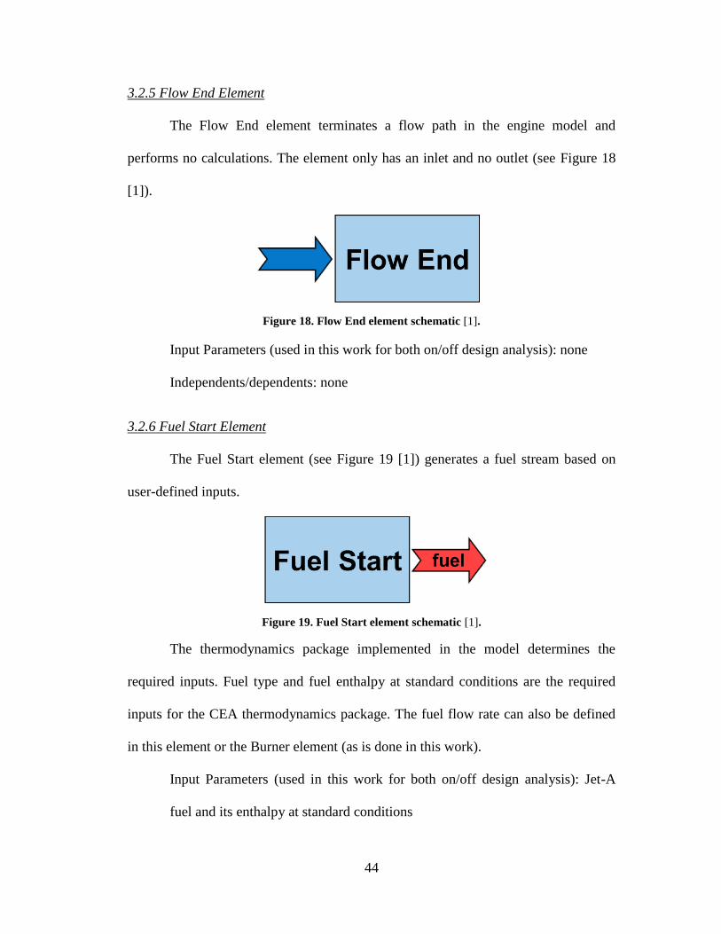
44
3.2.5 Flow End Element
The Flow End element terminates a flow path in the engine model and
performs no calculations. The element only has an inlet and no outlet (see Figure 18
[1]).
Figure 18. Flow End element schematic [1].
Input Parameters (used in this work for both on/off design analysis): none
Independents/dependents: none
3.2.6 Fuel Start Element
The Fuel Start element (see Figure 19 [1]) generates a fuel stream based on
user-defined inputs.
Figure 19. Fuel Start element schematic [1].
The thermodynamics package implemented in the model determines the
required inputs. Fuel type and fuel enthalpy at standard conditions are the required
inputs for the CEA thermodynamics package. The fuel flow rate can also be defined
in this element or the Burner element (as is done in this work).
Input Parameters (used in this work for both on/off design analysis): Jet-A
fuel and its enthalpy at standard conditions

45
Independents/dependents: none
3.2.7 Inlet Element
The Inlet element (see Figure 20 [1]) calculates performance of a typical gas
turbine inlet.
Figure 20. Inlet element schematic [1].
The ram pressure recovery (pressure ratio) is specified by the user as an input
value or calculation function. In this work, the ram recovery ( ) is defined as an
input parameter. It was assumed for this work that pressure losses in the inlet were
negligible ( = 1). The inlet exit pressure is calculated based on this value:
(23)
The ram drag force resulting from decelerating the flow is also output from this
element:
(24)
Input Parameters (used in this work for both on/off design analysis): ram
recovery
Independents/dependents: none
3.2.8 Inlet Start Element
The Inlet Start element (see Figure 21 [1]) creates an air stream to the engine
model.

46
Figure 21. Inlet Start element schematic [1].
Properties of the air stream (such as pressure, temperature, Mach number,
dynamic pressure, etc.) are defined/output in the Ambient element and are simply
referenced by this element. No calculations are performed in this element.
On-design analysis:
Input Parameters (used in this work): Ambient element’s name; air
flow rate (for second design case only)
Independents: air flow rate (for first design case only)
Dependents: none
Off-design analysis:
Input Parameters (used in this work): Ambient element’s name
Independents: air flow rate
Dependents: none
3.2.9 Nozzle Element
The Nozzle element (see Figure 22 [1]) calculates the performance of the gas
turbine’s nozzle.
Figure 22. Nozzle element schematic [1].

47
This element determines performance characteristics for different nozzle
geometries (convergent, convergent-divergent, fixed, or variable geometry). In on-
design mode, if the nozzle is not choked ( < ), the nozzle exit area
is calculated such that the calculated exhaust static pressure ( ) equals the
specified exhaust static pressure ( ). In this case, NPSS iterates Mach
number to match pressure using the ‘setStaticPs’ function. Stagnation exit pressure is
then determined from the exit static pressure and exit Mach number. If >
(choked flow), the exit area is calculated by setting the exit Mach number
equal to one. Static exit pressure is then determined using the ‘setTotal_hP’ function,
which iteratively calculates static pressure from the flow enthalpy, total exit pressure,
and Mach number. The nozzle is assumed to be adiabatic, so the exit stagnation
temperature is equal to the inlet stagnation temperature. In off-design mode, the
nozzle exit area is fixed from running the model in on-design mode. The exit Mach
number and pressure are then calculated as a function of that flow area and mass
flow. Again, the nozzle is assumed to be adiabatic.
For the second design case, mass flow rate into the nozzle is fixed based on
the specified air flow rate (determined from the first design case) and fuel flow rate
into the engine. For the first design case and all off-design cases, mass flow rate into
the nozzle must be adjusted by the system level solver. For this work, this is
accomplished by changing the air flow rate into the entire engine (via the Inlet Start
element). For both on-design and off-design mode, the gross thrust produced by the
engine is calculated from:

48
(25)
Note in Eq. (25) that the freestream velocity term ( ) is neglected because
the Olympus engine is tested under static conditions. The nozzle coefficient, , is
the ratio of the actual force produced divided by the theoretical force associated with
the momentum change. In this work, the default NPSS value of = 1 is used for
all model runs.
On-design analysis:
Input Parameters (used in this work):
o First design case: none
o Second design case: exhaust static pressure
Independents:
o First design case: exhaust static pressure
o Second design case: none
Dependents:
o First design case: physical exit area = calculated exit area;
measured thrust = calculated thrust
o Second design case: none
Off-design analysis:
Input Parameters (used in this work): none
Independents: exhaust static pressure
Dependents: physical exit area = calculated choked flow exit area;
measured thrust = calculated thrust

49
3.2.10 Shaft Element
The Shaft element performs (see Figure 23 [1]) work/power matching
between the compressor and turbine components of the gas turbine model.
Figure 23. Shaft element schematic [1].
Multiple torque producing components (compressors, turbines, etc.) can be
linked to a single shaft element. In this work, a single compressor and turbine element
are linked to the shaft. The input ports to the shaft must be declared by the user.
On-design analysis:
Input Parameters (used in this work): shaft input ports and shaft speed
Independents: none
Dependents: zero net torque on the shaft
Off-design analysis:
Input Parameters (used in this work): shaft input ports
Independents: shaft speed
Dependents: zero net torque on the shaft
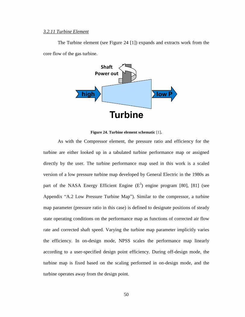
50
3.2.11 Turbine Element
The Turbine element (see Figure 24 [1]) expands and extracts work from the
core flow of the gas turbine.
Figure 24. Turbine element schematic [1].
As with the Compressor element, the pressure ratio and efficiency for the
turbine are either looked up in a tabulated turbine performance map or assigned
directly by the user. The turbine performance map used in this work is a scaled
version of a low pressure turbine map developed by General Electric in the 1980s as
part of the NASA Energy Efficient Engine (E3) engine program [80], [81] (see
Appendix “A.2 Low Pressure Turbine Map”). Similar to the compressor, a turbine
map parameter (pressure ratio in this case) is defined to designate positions of steady
state operating conditions on the performance map as functions of corrected air flow
rate and corrected shaft speed. Varying the turbine map parameter implicitly varies
the efficiency. In on-design mode, NPSS scales the performance map linearly
according to a user-specified design point efficiency. During off-design mode, the
turbine map is fixed based on the scaling performed in on-design mode, and the
turbine operates away from the design point.
51
To satisfy mass conservation, the inlet mass flow (the sum of the air and fuel
mass flows) is set equal to the outlet mass flow. The turbine exit pressure is
calculated based on the pressure ratio returned from the performance map or user-
defined input:
(26)
The exit enthalpy is calculated from the value of the isentropic efficiency
corresponding to the operating point in the turbine operating map and the definition
of isentropic efficiency [17]:
(27)
Power extracted from the flow is determined from the change in enthalpy:
(28)
The input parameters and independents/dependents used in this work are described
below.
On-design analysis:
Input Parameters (used in this work):
o First design case: pressure ratio
o Second design case: turbine performance map, efficiency, and
corrected shaft speed
Independents:
o First design case: efficiency
o Second design case: pressure ratio (turbine map parameter)
Dependents: none

52
Off-design analysis:
Input Parameters (used in this work): turbine performance map
Independents: pressure ratio (turbine map parameter)
Dependents: corrected mass flow = calculated mass flow from turbine
map
3.3 Solution Method
3.3.1 Numerical Solver
Thermodynamic models of gas turbine systems are described by highly
complex and nonlinear systems of differential equations. Explicit solutions to these
equations are generally impossible to develop. Therefore, iterative methods are often
employed that begin with an initial approximation of the solution that is refined in
subsequent iterations until a feasible solution is found.
The NPSS solver uses a modified Newton’s method [82] with Broyden
updates [82]–[84]. The first step of the iteration uses a finite-difference approach to
generate a Jacobian (a partial derivative matrix). Subsequent iterations use Broyden’s
method to update the Jacobian matrix in lieu of finite differencing. This improves
computational speed. More information about Newton’s and Broyden’s method can
be found in References [82]–[84].
As mentioned previously, the NPSS solver is configured with a set of
independents and dependents. The independents are varied by the solver to converge
on a solution that satisfies the dependent conditions. Perturbations to the independents
form the Jacobian matrix describing the correlations between all of the independents

53
and dependents in the model. During each iteration, NPSS calculates corrections to
the independents based on the current Jacobian and errors in the dependents returned
to the solver. New Jacobians are only generated after the first iteration according to
specific convergence criteria [76]. The user can specify the maximum number of
iterations and Jacobians for the solver to produce before the solver terminates and
convergence is not achieved.
3.3.2 Independents and Dependents
This section describes the NPSS solver configurations (independents and
dependents) used in the model of the Olympus turbojet. Two on-design cases are run
before running several off-design cases. A description of design versus off-design
analysis is provided later in Section “3.4 Cycle Analysis”. It is important to note here
that the current NPSS model is based on engine performance data without air flow
rate measurements. The method used to measure air flow rate in this work
significantly reduces freestream pressure and results in non-physical thrust
measurements. A more detailed discussion of the pressure losses through the air flow
measurement apparatus and its effect on thrust measurements will be presented in
Section “4.2 Challenges”.
As mentioned previously, AMT provided the compressor performance map
for the Olympus but they could not provide the turbine performance map. This
presents the difficulty of not knowing how the turbine’s pressure ratio and efficiency
change as a function of corrected shaft speed and corrected mass flow rate. As a
result, the approach taken involved scaling a General Electric’s low pressure turbine
map from NASA’s E3 program [81] (provided with the NPSS software release [76]).

54
However, scaling the map requires knowledge of the turbine design point efficiency.
This is estimated by first running the NPSS model without a turbine map and varying
the turbine efficiency, air flow rate, and nozzle exhaust static pressure to satisfy the
full throttle operation design conditions (defined in Section “3.4 Cycle Analysis”).
Table 6 lists the NPSS solver independents and dependents for the first design case.
Table 6. Independents and dependents for the design case without a turbine map.
Independents
Variable Name Description
AirControl air mass flow rate
TurbEff turbine efficiency
ExhPress exhaust static pressure
Dependents
Variable Name Description
ShH.integrate_Nmech zero net torque on the shaft
Thrust specified net engine thrust = calculated thrust
NozArea specified nozzle exit area = calculated nozzle
exit area
The second design case runs the model again but with the low pressure turbine
map using input values of turbine efficiency (now the design value), air flow rate, and
exhaust static pressure from the converged solution in the first design case. Table 7
lists the independents and dependents for the second design case.
Table 7. Independents and dependents for the design case with the low pressure turbine map.
Independents
Variable Name Description
TurbH.S_map.ind_parmMap turbine map pressure ratio
Dependents
Variable Name Description
ShH.integrate_Nmech zero net torque on the shaft
Although the solver configuration is different between the first and second
design cases, it is important to note that the converged solutions are the same. The
input parameters for both design cases are defined in the following section. Recall

55
that the current model is based on performance data without air flow measurements;
otherwise, air flow rate would be an input to the model instead of being varied by the
solver as an independent.
In this work, off-design cases are run to predict engine performance at
different throttle settings (specified by the user as percentages of the full throttle
design condition thrust). As with the second design case, off-design cases are run
using the low pressure turbine map to predict turbine performance. Table 8 shows the
NPSS solver configuration for the off-design cases.
Table 8. Independents and dependents for off-design cases.
Independents
Variable Name Description
InletStart.ind_W (same as AirControl) air mass flow rate
CmpH.S_map.ind_RlineMap compressor map operating line parameter
TrbH.S_map.ind_parmMap turbine map pressure ratio
ShH.ind_Nmech shaft speed (RPM)
ExhPress exhaust static pressure
Dependents
Variable Name Description
CmpH.S_map.dep_errWc corrected mass flow = calculated mass flow
from compressor map
TrbH.S_map.dep_errWp corrected mass flow = calculated mass flow
from turbine map
NozPri.dep_Area physical exit area = calculated choked flow exit
area
ShH.integrate_Nmech zero net torque on the shaft
Thrust specified net engine thrust = calculated thrust
The NPSS solver is generally defined using the ‘autoSolver Setup()’
command, which automatically adds independents and dependents to the solver based
on the components included in the gas turbine model. Newly user-defined or existing
independents and dependents can be added or removed from the solver at the user’s
discretion after calling the ‘autoSolverSetup()’ command. For the design cases in this
work, this command only adds the ‘TrbH.S_map.ind_parmMap’ independent and

56
‘ShH.integrate_Nmech’ dependent to the solver. The other independents/dependents
listed in Table 6 are newly defined. For the off-design cases in this work, the
‘autoSolverSetup()’ command adds all of the independents/dependents described in
Table 8 to the solver except for the ‘ExhPress’ independent and ‘Thrust’ dependent.
One of the challenges associated with NPSS solver setup is ensuring that there are
equal numbers of independents and dependents. In many instances, the user will need
to provide additional independents/dependents to satisfy this requirement. The
difficulty becomes defining independents/dependents that have physical significance
to the engine model and ensuring that all the dependents are affected by at least one
of the independents.
3.4 Cycle Analysis
Cycle analysis in NPSS is generally performed in two stages: a design case
(design analysis/on-design mode) followed by one or more off-design cases (off-
design analysis/off-design mode). The design case determines all geometric/sizing
parameters (such as the nozzle throat/exit area) and turbomachinery performance map
scale factors based on the specified design parameters. The design case establishes
the baseline engine model and serves as a reference condition for off-design analysis.
In this work, the only geometric parameter calculated during a design case is the
nozzle exit area. The solver dependent ‘NozArea’ in the first design case ensures that
the calculated nozzle exit area equals the physical engine’s nozzle exit area of 33.23
cm2. This nozzle exit area remains fixed for the second design case and all off-design
cases.

57
Generally, only one design case is required for each model run. The reasons
for executing two design cases in this work were discussed above in Section “3.3.2
Independents and Dependents”. The input design case parameters for the Olympus
are shown in Table 9.
Table 9. Full throttle design case parameters for the Olympus engine model.
Parameter Value
Ambient Pressure (kPa) 101.97
Ambient Temperature (K) 296.53
Shaft Speed (RPM) 108,500
Thrust (N) 210.8
Mach Number 0
Ram Pressure Recovery 1.0
Compressor Total Pressure Ratio (P03/P02) 3.78
Compressor Efficiency 0.72
Fuel Type Jet A
Fuel Enthalpy (kJ/kg) -1813.3
Fuel Flow Rate (kg/sec) 0.0112
Burner Pressure Loss 4.83%
Burner Efficiency 0.95
Turbine Total Pressure Ratio (P04/P05) 2.26
Nozzle Exit Area (cm2) 33.23
The design case parameters are defined for full throttle operation. The input
values of ambient pressure, ambient temperature, engine speed, thrust, Mach number,
compressor pressure ratio, fuel flow rate, burner pressure loss, and turbine pressure
ratio are determined experimentally from full throttle operation of the Olympus.
Compressor efficiency is estimated from the compressor performance map provided
by AMT. The fuel enthalpy was calculated for liquid Jet-A from thermodynamic data
available with the NPSS software package [76]. Also, the parameters defined in Table
9 are specifically for the first design case mentioned in Section “3.3.2 Independents
and Dependents”. The input values of turbine efficiency, air flow rate, and exhaust

58
static pressure for the second design case are determined from the converged solution
of first design case. All other input parameters for the second design case are the
same as those listed in Table 9.
During off-design cases, NPSS calculates operating characteristics for
conditions other than those defined in the design case. For example, the user can
specify different ambient conditions, flight Mach number, throttle settings, etc. In this
work, the performance of the Olympus engine is predicted for various throttle
settings. Input parameters for off-design analysis are percent throttle, ambient
pressure, ambient temperature, fuel flow rate, and burner pressure drop. It is
important to note that the engine model is fixed for the off-design analysis according
to the converged solution of the design analysis. This means performance is
calculated using the same turbomachinery performance maps and geometric engine
parameters for each case. If several cases were run in on-design mode to meet each
measured operating point for the Olympus, then each case would result in a
completely different engine. This is because NPSS scales the compressor/turbine
maps and calculates the nozzle exit area differently for each operating point when run
in on-design mode. For this reason, gas turbine models in NPSS are usually run with
a design case followed by multiple off-design cases (as is done in this work).
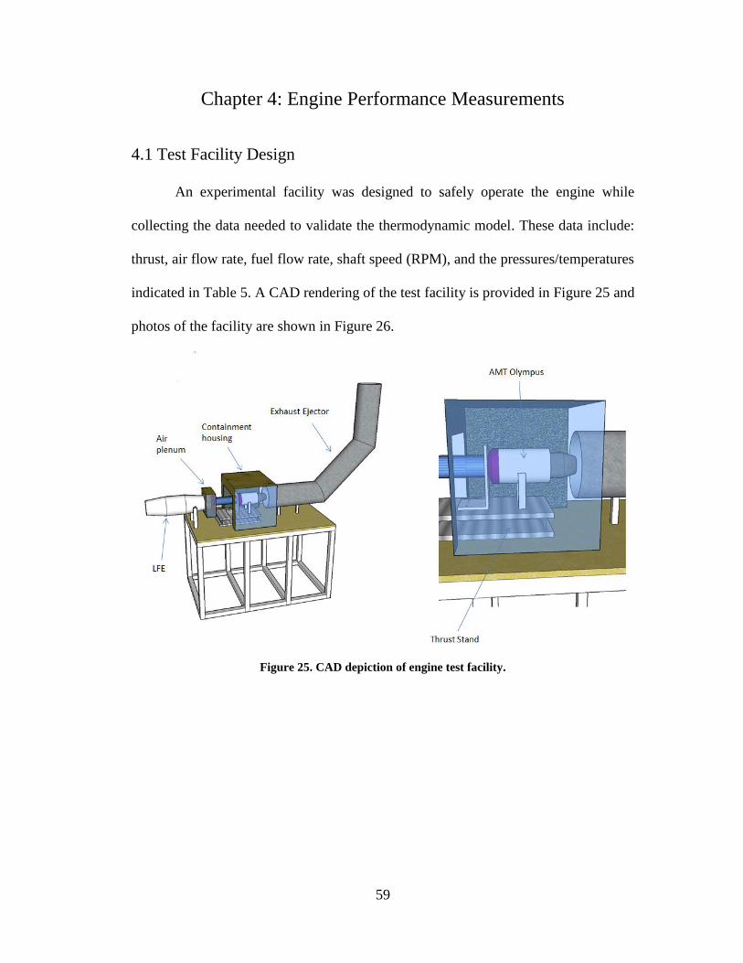
59
Chapter 4: Engine Performance Measurements
4.1 Test Facility Design
An experimental facility was designed to safely operate the engine while
collecting the data needed to validate the thermodynamic model. These data include:
thrust, air flow rate, fuel flow rate, shaft speed (RPM), and the pressures/temperatures
indicated in Table 5. A CAD rendering of the test facility is provided in Figure 25 and
photos of the facility are shown in Figure 26.
Figure 25. CAD depiction of engine test facility.

60
Figure 26. Engine test facility.
The engine sits in a containment housing that protects the laboratory and its
occupants from debris in case of catastrophic failure. The housing was designed with
dimensions large enough to allow modifications to the engine for eventual fuel cell
integration. Fireproof denim insulation covers the interior walls of the housing to
reduce engine noise for indoor operation. The engine rests on a thrust stand that
measures force along the same axis as incoming airflow. The thrust stand consists of
a horizontal aluminum plate supported by thin metal flexures and is restrained by a
load cell. More details about the design of the thrust stand can be found in [85]. An
aluminum duct connects the engine inlet to the air plenum, and the duct is connected
to the air plenum using a compliant rubber gasket material. An ejector nozzle cools

61
the engine’s exhaust prior to entering the laboratory’s exhaust hood by mixing it with
room temperature air.
4.2 Challenges
The most challenging aspect of the test facility design is ensuring the air flow
rate measurement does not disrupt the thrust measurement. An accurate air flow rate
measurement requires all incoming air to flow through the laminar flow element
(LFE). This necessitates creating an air tight seal between the LFE exit and engine
inlet that is still flexible enough to transmit thrust. This proved to be difficult because
the inlet cowl of the Olympus contains several essential connection and electronic
ports (for fuel lines, RPM sensor, electric starter, etc.). Ultimately, this was
accomplished by attaching the downstream end of the laminar flow element to a small
plenum and connecting the engine to the other side of the plenum using a custom inlet
extension that attaches to a flexible rubber diaphragm as illustrated in Figure 27.
Figure 27. Custom inlet extension.
The rubber diaphragm is intended to allow the thrust stand to deflect as load is
applied. The inlet extension contains two feed-through holes for the fuel lines and a
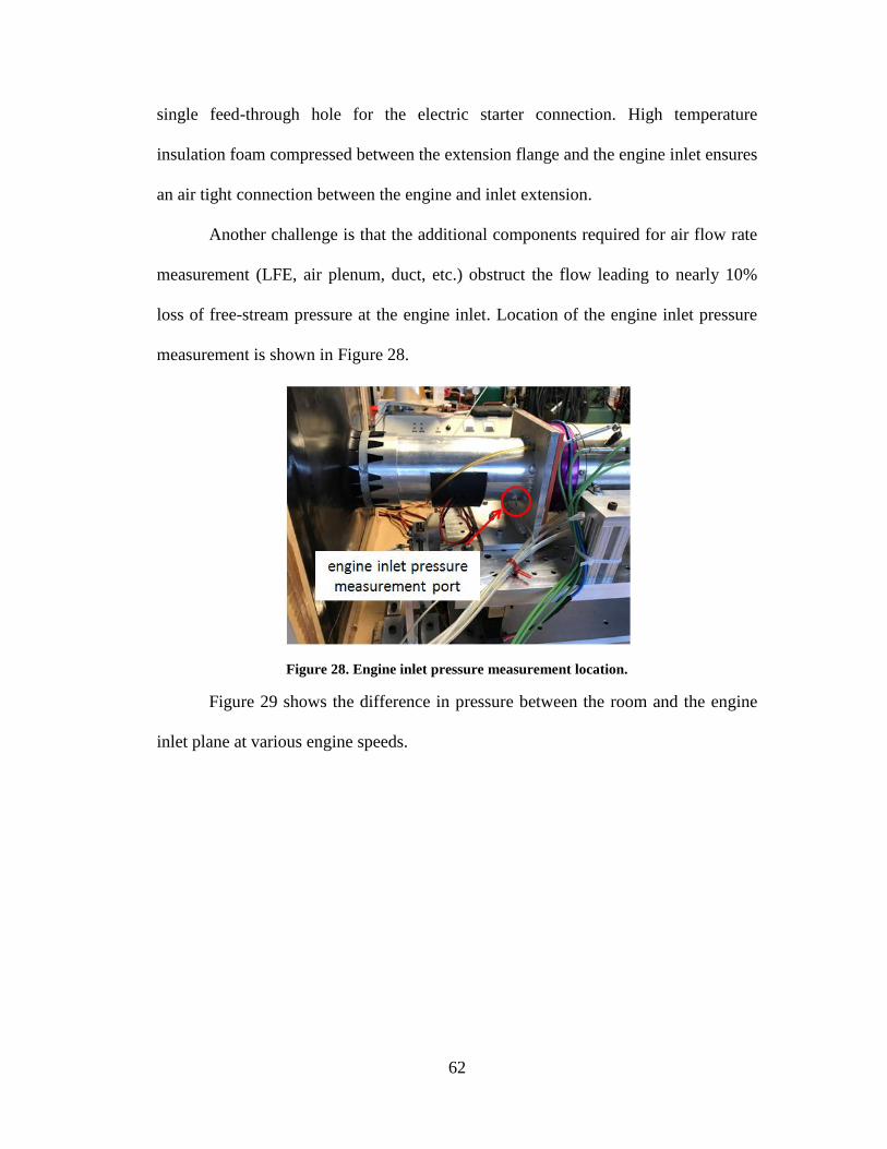
62
single feed-through hole for the electric starter connection. High temperature
insulation foam compressed between the extension flange and the engine inlet ensures
an air tight connection between the engine and inlet extension.
Another challenge is that the additional components required for air flow rate
measurement (LFE, air plenum, duct, etc.) obstruct the flow leading to nearly 10%
loss of free-stream pressure at the engine inlet. Location of the engine inlet pressure
measurement is shown in Figure 28.
Figure 28. Engine inlet pressure measurement location.
Figure 29 shows the difference in pressure between the room and the engine
inlet plane at various engine speeds.

63
Figure 29. Pressure drop across LFE-plenum-duct as a function of engine speed.
Figure 29 shows the pressure drop through the LFE-plenum-duct is quite large
(~9.4% P∞ at full throttle). Most of this pressure loss occurs in the plenum and duct as
the pressure drop across the LFE is relatively small (~1.5% at full throttle) (see
Figure 30).

64
Figure 30. Pressure drop across the LFE as a function of engine speed.
Despite these pressure losses, measured thrust is consistently greater at each
engine speed than measured thrust without the obstructive air flow measurement
apparatus (see Section “5.2.4 Thrust with & without Air Flow Rate Measurement”).
Another complication with the test facility design is thrust stand calibration. It
was observed that the calibration curves for the thrust stand change over the course of
an engine throttle sweep (see Figure 31). In Figure 31, the colored lines represent the
calibration curves for different speeds during a throttle sweep. The term ‘throttle
sweep’ simply refers to a set of engine runs between 20% and 100% throttle.
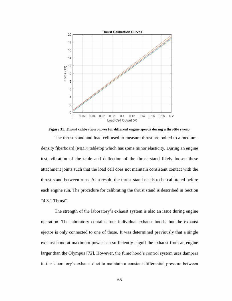
65
Figure 31. Thrust calibration curves for different engine speeds during a throttle sweep.
The thrust stand and load cell used to measure thrust are bolted to a medium-
density fiberboard (MDF) tabletop which has some minor elasticity. During an engine
test, vibration of the table and deflection of the thrust stand likely loosen these
attachment joints such that the load cell does not maintain consistent contact with the
thrust stand between runs. As a result, the thrust stand needs to be calibrated before
each engine run. The procedure for calibrating the thrust stand is described in Section
“4.3.1 Thrust”.
The strength of the laboratory’s exhaust system is also an issue during engine
operation. The laboratory contains four individual exhaust hoods, but the exhaust
ejector is only connected to one of those. It was determined previously that a single
exhaust hood at maximum power can sufficiently engulf the exhaust from an engine
larger than the Olympus [72]. However, the fume hood’s control system uses dampers
in the laboratory’s exhaust duct to maintain a constant differential pressure between

66
the duct and the lab which prevents the exhaust hoods from operating at maximum
power. At engine speeds upwards of about 40% throttle, the fume hood cannot keep
up with the exhaust expelled from the engine. All four hoods must be powered on
between runs at these higher speeds and allowed to run for approximately 10-15
minutes to remove residual engine exhaust from the lab. Failure of the exhaust ejector
to keep up with the engine’s exhaust during runs presumably results in backpressure
which could have adverse effects on thrust.
4.3 Measured Quantities
4.3.1 Thrust
Engine thrust is measured using a Transducer Techniques ESP-35 load cell
with a maximum capacity of 77 lbf (343 N). The ESP-35 is a cantilever beam load
cell with an accuracy of +/- 1.0% of the load cell reading. The contact point between
the load cell and the top horizontal plate of the thrust stand is a single hex bolt (see
Figure 32). Prior to each engine run, the hex bolt was tightened against the top plate
of the thrust stand with about 3 lbf (13.3 N) of preload tension measured on the load
cell to ensure secure contact between the load cell and thrust stand. Output from the
ESP-35 is filtered using a Transducer Techniques TMO-2-160 load cell conditioner.

67
Figure 32. Thrust stand load cell configuration.
Although the load cell itself was calibrated by the manufacturer, some
accounting is needed for the stiffness of the thrust stand flexures and LFE-to-engine
connection. As a result, the thrust measurement system must be calibrated to account
for the effective spring constant produced by these added components. The thrust
stand is calibrated using a cable/pulley system where weights are hung at the end of
the cable (see Figure 33).

68
Figure 33. Calibration pulley system.
A calibration curve relating thrust produced by the engine as a function of
load cell voltage output must be produced at the beginning of each testing session due
to the elasticity of the MDF tabletop. The procedure for generating a calibration curve
for the thrust measurement system is outlined below:
1. Remove all weights from the cable/pulley system, and zero the load cell
output using the “Balance” knob on the TMO-2-160 load cell signal
conditioner.
2. Hang different (known) weights from the end of the loading cable, and record
both the total force exerted on the thrust stand and voltage output from the
load cell.
3. Incrementally unload pulley system, and record the net force on the thrust
stand and load cell voltage output for each weight removed.
4. Repeat steps 2-3 about two or three times.
5. Plot force as a function of load cell voltage output, and generate a linear
regression curve. A typical calibration plot is shown in Figure 34.

69
Figure 34. Example thrust stand calibration curve.
To produce the plot in Figure 34, known weights were loaded and unloaded
onto the pulley system. The calibration data show there is some hysteresis in the
thrust measurement system which is why the thrust stand needs to be calibrated
before each engine run.
4.3.2 Air Flow Rate
The Olympus engine draws air through a Meriam Z50MC2-6 LFE. The
maximum flow rate of the Z50MC2-6 is 1000 SCFM (33.9 kg/min) and corresponds
to a pressure drop of 8 in H2O (203.2 mm H2O). The instrument’s accuracy is +/-
0.72% to +/- 0.86% of the measured value. A manufacturer-provided calibration
curve is used with the measured pressure drop across the laminar flow element to
calculate air mass flow rate.
The volumetric flow rate is calculated using the quadratic calibration curve
provided by the manufacturer:
(29)

70
where and are calibration coefficients provided by Meriam (see Table 10), is
the measured differential pressure across the LFE, is the viscosity of air at the
incoming flow temperature, and is the viscosity of air at 70°F (21.1°C) (in
micropoise).
Table 10. Calibration coefficients for LFE.
Coefficient Value
1.1997661e2
-6.0838751e-1
The pressure drop across the laminar flow element ( ) is measured using an
Omega PX277-30D5V differential pressure transducer with a full-scale range of 30 in
H2O (762 mm H2O). Multiplying the volumetric flow rate by the ratios of temperature
and pressure to standard temperature and pressure gives the volumetric flow rate at
standard conditions:
(30)
where is the standard temperature of 70°F (21.1°C), is the incoming flow
temperature, is the ambient (room) pressure, and is the standard pressure of
29.92 in Hg (759.97 mm Hg). Ambient pressure was recorded from the National
Weather Service’s website [86] for College Park Airport at the time of testing.
Finally, the air mass flow rate is determined by multiplying the standard volumetric
flow rate by the density of air at standard conditions, :
(31)

71
4.3.3 Fuel Flow Rate
A gravimetric system is used to measure the fuel flow rate (see Figure 35).
The fuel tank is suspended from a Transducer Techniques ESP-20 cantilever beam
load cell with a maximum load capacity of 44 lbf (196 N) and an accuracy of +/-
1.0% as illustrated in Figure 35. Like the thrust stand load cell, output from the ESP-
20 is filtered using a Transducer Techniques TMO-2-160 signal conditioner. At the
beginning of each testing session, the load cell is zeroed (with the unistrut cage and
fuel tank attached) in the same manner as the thrust stand load cell.
Figure 35. Gravimetric fuel weight measurement system.
During engine runs, the weight of the fuel is logged as a function of time.
After the experiment is over, a linear regression curve is fit to the results. The slope of
the curve is the equivalent fuel flow rate. An example of fuel weight plotted versus

72
time and its corresponding linear regression curve for an engine test at 80% throttle is
shown in Figure 36.
Figure 36. Fuel weight vs. time for a single engine run at 80% throttle.
For the fuel weight data in Figure 36, the equivalent fuel flow rate is 0.0193
lbf/sec (or 0.00875 kg/sec).
4.3.4 Temperatures
Ambient and axial engine stage temperature measurements are made using K-
Type thermocouples provided by AMT with the Olympus engine. Unfortunately,
AMT could not disclose the manufacturer of these thermocouples. Output from the
thermocouples is recorded in units of °C. Assuming the error limits of the AMT-
supplied thermocouples are similar to those of K-Type thermocouples manufactured
by Omega [87], the accuracy of the thermocouples is assumed to be roughly +/-
0.75% of the measured value. Refer to the schematic drawing of the Olympus (Figure
12) for the location of the temperature measurement ports and the orientation of the
thermocouples in the flow. The engine’s hot section thermocouples (T04 and T05) need
to be corrected for losses due to conduction and radiation. This is discussed later in

73
Section “4.4 Thermocouple Corrections”. The exhaust gas temperature (T06) is
displayed by the engine’s electronic data terminal (EDT), and its signal cannot be
recorded directly. This is because the T06 thermocouple is a required input to the
engine’s electronic control unit (ECU) for proper start-up and shutdown sequences.
T06 was recorded by hand during engine testing.
4.3.5 Pressures
The Olympus in “University Configuration” only came equipped with axial
engine stage pressure measurements ports and not sensors to make these
measurements. Refer to the schematic drawing of the Olympus (Figure 12) for the
location of the pressure measurement ports and their orientation in the flow. Pressure
measurements are made using Omega PX309-100A5V absolute pressure transducers
with a range of 0-100 psia (0-689 kPa) and an accuracy of +/- 0.25% of the measured
value. Festo tubing supplied with the engine is inserted into the measurement ports on
the engine and connected to the pressure transducers. Again, ambient pressure was
simply recorded from the National Weather Service’s website [86] for College Park
Airport.
4.3.6 Engine Speed
The Olympus comes equipped with a pre-installed RPM sensor at the
compressor stage of the engine. RPM readings from the sensor are displayed on the
engine’s electronic data terminal (EDT). The EDT also indicates percent throttle as
controlled by the analog throttle knob. The RPM and percent throttle readings from
the EDT were recorded by hand during each engine run.

74
4.3.7 Data Acquisition
A National Instruments NI 9205 analog input module and a NI 9213
thermocouple module installed in a cDAQ-9178 chassis logs all measurements
(excluding ambient pressure, T06, RPM, and percent throttle) at 10 Hz. Five throttle
sweeps spanning 20% to 100% throttle were performed. This provided five data
points for each operating condition which are used to compute the averages presented
later in this work. For each data point, raw measurements (excluding fuel weight) are
averaged over the testing period which generally lasted about 60 seconds. At a
sampling rate of 10 Hz, this means that each data point (excluding fuel flow rate)
represents an average of approximately 600 raw measurements.
4.3.8 Summary of Measurements
Table 11 shows all measured quantities in this work.
Table 11. Summary of measured quantities.
Measured Quantity Measuring Device
Thrust Transducer Techniques ESP-35 load cell
Air Flow Rate (Pressure Drop)
Meriam Z50MC2-6 laminar flow element;
Omega PX277-30D5V differential pressure
transducer
Fuel Flow Rate (Fuel Weight) Transducer Techniques ESP-20 load cell
Ambient Temperature (Tamb) K-Type thermocouple
T03 K-Type thermocouple
T04 K-Type thermocouple
T05 K-Type thermocouple
T06 K-Type thermocouple
Ambient Pressure (Pamb) National Weather Service’s website for
College Park Airport
Ps3 Omega PX309-100A5V pressure transducer
P03 Omega PX309-100A5V pressure transducer
P04 Omega PX309-100A5V pressure transducer
P05 Omega PX309-100A5V pressure transducer
Engine Speed (RPM) Engine ECU/EDT
% Throttle Engine ECU/EDT

75
4.4 Thermocouple Corrections
The measured values of the turbine inlet temperature (T04) and turbine exit
temperature (T05) in this work are significantly lower than the NPSS predicted values.
This is probably due to conduction and radiation losses in the T04 and T05
thermocouples. The discrepancy between predicted theoretical and measured
temperatures in the hot sections of the Olympus in “University Configuration” was
also observed by Prof. Harald Funke3, who provided preliminary performance data to
assist initial efforts in testing the NPSS model before the experiments were
completed. Bakalis and Stamatis [30] made this observation as well. Conduction and
radiation loss corrections in this work are calculated by modeling the T04 and T05
thermocouple sheaths as pin fins in a cross flow [88]–[90].
4.4.1 Pin Fin Model
The K-Type thermocouples provided by AMT consist of a thin stainless steel
sheath that protects the sensor lead wires. These thermocouple sheaths protrude
directly into the flow of the engine (see Figure 37).
3 Professor, Aachen University of Applied Sciences, Aachen, Germany

76
Figure 37. Sheathed thermocouple orientation in flow.
Temperature measurement error is due to axial conduction along the length of
the sheath, radiation heat transfer between the sheath and the engine walls, and
convection between the sheath and gas. This causes under-prediction of the true gas
temperature. A simple method of estimating the measurement error involves
modeling the sheathed thermocouple as a pin fin [88]–[90] (see Figure 38).
Figure 38. Thermocouple well pin fin model.
The particular approach used in this work for estimating thermocouple
temperature measurement errors follows that of [90]. It is assumed that the cross-
sectional area of the sheathed thermocouple assembly (effectively the pin) is

77
significantly larger than that of the thermocouple lead wires, so conduction through
the wires themselves can be neglected. It is also assumed that the temperature of the
sheath is between that of the gas and the wall so that it is heated by convection from
the gas and cooled by radiation to the engine walls. The radiation heat flux from the
gas to the sheath is approximated using a linearized model [90]:
(32)
where the radiation heat transfer coefficient, , is given by:
(33)
The linearized form of the radiation heat flux in equation (32) can be used
here because it is assumed that the temperature at any point along the thermocouple
sheath ( ) is of the same order of magnitude as the temperature of the wall ( ) [91].
The greatest difference between and occurs when considering the sheath tip
temperature ( ) at full throttle engine operation. At 100% throttle, 1050 K and
is assumed to be 450 K at the turbine inlet, and 950 K and is assumed to
be 600 K at the turbine exit. Here, the values of are the raw measured
(uncorrected) temperatures at the turbine inlet/exit, and the values of are the
assumed wall temperatures at the turbine inlet/exit (see Section “4.4.3 Parameters for
the Thermocouple Corrections”).
The temperature correction is determined by performing an energy balance on
the differential sheath element illustrated in Figure 39.
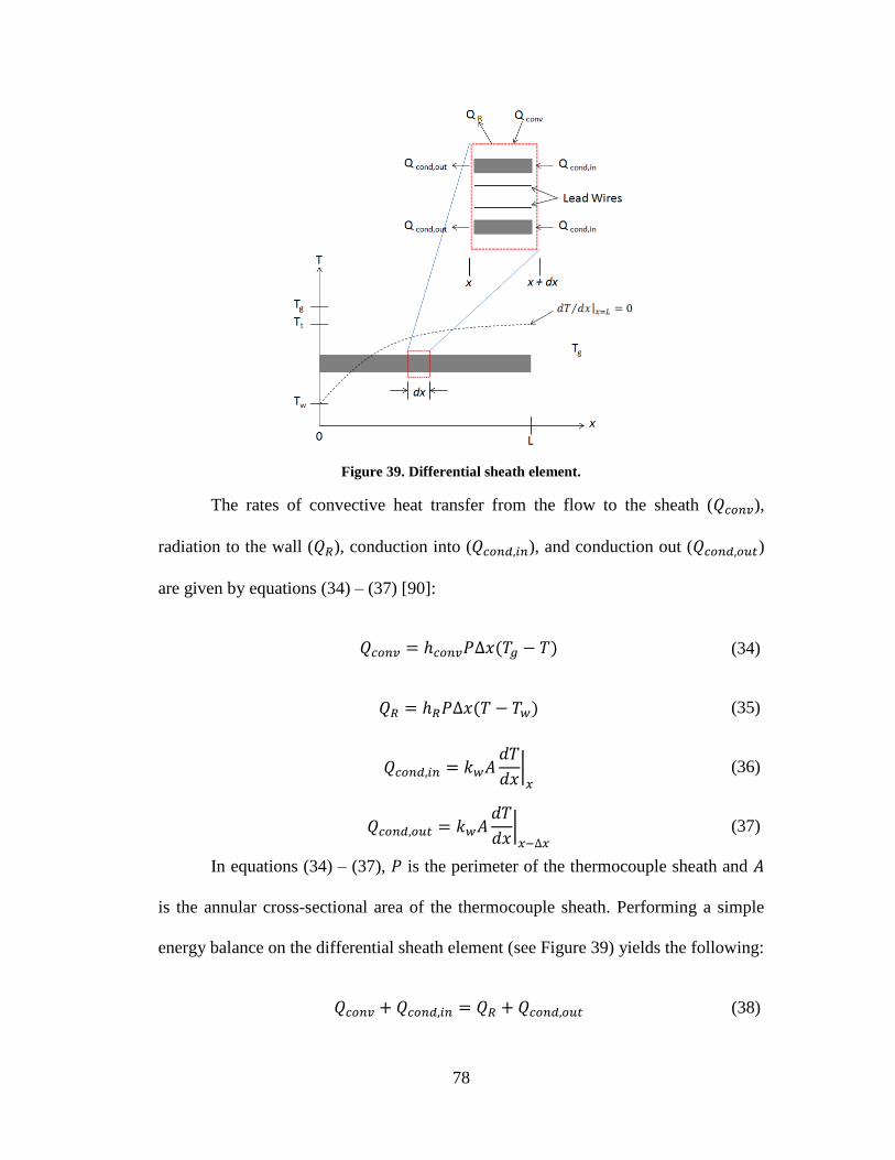
78
Figure 39. Differential sheath element.
The rates of convective heat transfer from the flow to the sheath ( ),
radiation to the wall ( ), conduction into ( ), and conduction out ( )
are given by equations (34) – (37) [90]:
(34)
(35)
(36)
(37)
In equations (34) – (37), is the perimeter of the thermocouple sheath and
is the annular cross-sectional area of the thermocouple sheath. Performing a simple
energy balance on the differential sheath element (see Figure 39) yields the following:
(38)

79
Substituting equations (34) – (37) into equation (38) yields a second order
differential equation for the sheath temperature ( ) as a function of distance along the
sheath ( ) where the tip is at [90]:
(39)
Equation (39) can rewritten in terms of a reference temperature, and
effective fin parameter, [90]:
(40)
where and is defined as [90]:
(41)
The reference temperature, , is defined as [90]:
(42)
Assuming an insulated boundary condition at the sheath tip ( ),
equation (40) can be solved for the indicated thermocouple temperature [90]:
(43)
where and is the temperature at the tip of the sheath. Finally, the
thermocouple measurement error ( ) is given by [90]:
(44)
Solving for the true gas temperature ( ) in equation (44) gives:
(45)

80
This analysis shows that the measurement error (Eq. (44)) decreases with
increasing immersion depth ( ), decreasing thermal conductivity, decreasing
emissivity, and increasing fluid velocity.
4.4.2 Determining the Convective Heat Transfer Coefficient
Calculating as described above requires an estimate of the convective heat
transfer coefficient ( ). It is defined as [88]:
(46)
where is the Nusselt number, is the thermal conductivity of the gas, and is the
thermocouple sheath immersion depth into the flow. is estimated using the
Zhukaskas correlation for a cylinder in a cross flow [90]:
(47)
where the constants and are dependent on Reynolds number ( ) and is
dependent on Prandtl number ( ). Values for these constants used in this work are
given in the next section.
4.4.3 Parameters for the Thermocouple Corrections
The parameters used to calculate the thermocouple corrections in this work
are presented in Table 12.

81
Table 12. Parameters used to calculate T04 and T05 thermocouple corrections.
Constants
Parameter Description Value Units Ref.
Stefan-Boltzmann constant 5.67e-8 W/m2/K
4 [88]
Ideal gas constant for air 287 J/kg-K [88]
Thermocouple sheath perimeter 12.47 mm
Thermocouple sheath conduction area 10.52 mm2
Zhukaskas Correlation Parameters
Parameter Description Value Units Ref.
Zhukaskas correlation constant 0.26 [90]
Zhukaskas correlation constant 0.6 [90]
Zhukaskas correlation constant 0.36 [90]
Prandtl number 0.7
T04 Correction
Parameter Description Value Units Ref.
Wall emissivity 0.75 [88]
Thermocouple sheath thermal conductivity 20.0 W/m/K [88]
Thermocouple sheath immersion length 17.1 mm
Assumed wall temperature 450 K
T05 Correction
Parameter Description Value Units Ref.
Wall emissivity 0.75 [88]
Thermocouple sheath thermal conductivity 18.0 W/m/K [88]
Thermocouple sheath immersion length 7.94 mm
Assumed wall temperature 600 K
Values for turbine inlet/exit wall emissivity and thermocouple sheath wall
thermal conductivity were estimated from available data for stainless steel [88].
Similarly, values for dynamic viscosity and thermal conductivity of the gas ( ) used
to calculate the convective heat transfer coefficient ( ) were estimated from
tabulated data for air as a function of temperature [88].
Thermocouple corrections at the compressor exit (T03) and nozzle exit (T06)
were not computed. The user’s manual [92] of the Olympus states that the inlet casing
at the compressor generally reaches a temperature of about 400 K. The raw measured
T03 temperatures ranged between 360 K and 480 K for all engine speeds considered.

82
Because the raw measured T03 values are relatively close to the compressor wall
temperature, the corrections calculated according to the analysis above would be
minimal. The results reported later in this work suggest this was a reasonable
assumption. T06 was not corrected because the exhaust pressure is not measured in
this work. The exhaust pressure is required for an estimate (and hence and
).
4.5 Estimating Uncertainty
This section describes the uncertainties in the measured and calculated
quantities reported in this work. Uncertainties are indicated in the results section with
error bars that represent a 95% confidence interval for each measured/calculated data
point.
4.5.1 Measurement Uncertainty
Measurement error consists of two components: random error and systematic
error. Random errors are random deviations around the mean and can be reduced by
increasing the number of samples. Systematic errors are the component of the total
error that has to do with the instrument/measurement method itself and remain
constant during repeated measurements [93]. In this work, the random component of
the error is taken to be the standard deviation about the mean, [93]:
(48)
where is the ith
measurement of the quantity of interest, is the mean of the
measured quantity based on samples, and is the standard deviation of

83
samples. Since five throttle sweeps were conducted, there are 5 performance
measurements at each engine speed and thus = 5.
Systematic errors arise primarily from the accuracy, linearity and repeatability
limits of the sensors used to make measurements (thermocouples, pressure
transducers, load cell, thrust balance, etc.). The total systematic uncertainty, , is
calculated using [93]:
(49)
where … are the systematic errors in the measurements (such as linearity and
repeatability limits of the sensors). The total measurement uncertainty ( ) for a 95%
confidence level for a measurement is given by [93]:
(50)
where is the systematic error and is the standard deviation of the mean. The true
value of the measurement ( ) is then reported as:
(51)
where is the mean given by:
(52)
where is the measurement, and is the number of data points.
4.5.2 Uncertainties in Calculated Results
The total error in calculated results is also comprised of random and
systematic components. As with measured quantities, the random error of a result is
calculated using the standard deviation of the mean for repeated tests [93]:

84
(53)
where is the standard deviation of the sample, is the mean of the calculated
result, is the calculated result, and is the total number of tests performed.
Systematic error ( ) in a quantity calculated using measured quantities is
given by [93]:
(54)
where is the systematic error of the measured parameter determined using
equation (49). The symbol is the sensitivity coefficient of the measured parameter
and is defined as:
(55)
where is the calculated result.
The total uncertainty of a result with 95% confidence is then:
(56)
where is the total systematic error in the result, and is the standard deviation
about the mean. The true value of the result ( ) is then expected to be:
(57)
where is the mean result calculated using equation (52).

85
4.6 Experimental Procedures
This section outlines the procedures used to measure the performance of the
Olympus engine. A more detailed discussion of the engine’s operation and
troubleshooting is provided in the user’s manual for the Olympus [92].
4.6.1 Preparing the Engine
1. Ensure that the engine battery is fully charged or at least has sufficient charge
for the engine’s ECU to initiate the start-up sequence (refer to user’s manual
[92] for the minimum charge required for start-up). It is good practice to have
the battery as close to fully charged as possible for proper ECU function.
2. Ensure that all inputs (electric starter, T06 thermocouple, fuel pump, throttle
controller, RPM sensor, etc.) to the ECU are securely connected. It is also
important to make sure the throttle controller is communicating properly with
the ECU (refer to “Dual Channel Operation” in the user’s manual [92]).
3. Ensure that there is enough fuel in the fuel tank. The fuel is a mixture of 95%
Jet-A and 5% AeroShell 500 turbine oil. Make sure the fuel lines are securely
connected to the engine and there are no leaks.
4. Inspect the engine for any damage prior to start-up.
4.6.2 Preparing the Test Facility
1. Ensure that all thermocouples attached to the engine are securely connected,
and make sure the tubing connecting the pressure measurement ports on the
engine to the pressure transducers is intact.
2. Place the containment housing over the engine and thrust stand, and turn on
the fume hood attached to the exhaust ejector. Make sure that all of the other

86
hoods in the lab are off. Note that it takes a few minutes for the hood to
achieve maximum power.
3. Turn on both load cell signal conditioners (i.e., for the thrust and fuel flow
rate measurements), the power supply for the pressure transducers, and the
LabView modules. Allow this equipment roughly 10 minutes to warm-up.
This is particularly important for the load cell signal conditioners prior to
calibration.
4. Ensure the wiring for all measuring devices is properly configured.
5. Calibrate the thrust stand according to the procedure described in Section
“4.3.1 Thrust”.
The engine and test facility are now ready for data collection.
4.6.3 Data Collection
1. Switch on the engine’s ECU. When the engine’s EDT indicates the engine is
ready for start-up, initiate the start-up sequence. Refer to the user’s manual
[92] for interpretation of the EDT’s graphic display and how to initiate start-
up. After successful start-up, the ECU will automatically throttle the engine to
idle (~36,000 RPM).
2. Once the engine achieves idle RPM, adjust the throttle knob to the desired
throttle setting. Throttle setting is displayed on the EDT as a percentage of
maximum thrust.
3. Allow the engine to equilibrate for about 60 seconds after each throttle change
before acquiring data.

87
4. After about 60 seconds of data collection, stop recording data. During the data
collection period, be sure to record the engine’s RPM and throttle setting from
the engine’s EDT. The speed and percent throttle should remain fixed over the
data collection period.
5. Initiate the engine’s automatic shut-down sequence (refer to user’s manual
[92]). During the shut-down sequence, the ECU will rotate the compressor
until T06 cools to the desired temperature. During this time, turn on all hoods
in the lab to expel any residual exhaust present in the lab.
6. Once the ECU stops rotating the compressor, switch off the ECU. The engine
is now completely powered off.
7. To run the engine again at a different throttle setting, repeat the steps in this
section (“4.6.3 Data Collection”). Allow roughly 10 minutes between each
engine run for the fume hoods to remove any exhaust present in the lab.
Remember to turn off all hoods except for the one attached to the exhaust
ejector before the next run. Also, make sure the engine’s battery has sufficient
charge and there is enough fuel for the next run.
4.6.4 Safety
The engine operator and close observers should wear hearing and eye
protection at all times during engine operation. Other lab occupants should at least
wear hearing protection. Any debris or light and loose objects should be kept away
from the engine’s inlet (this includes fuel lines and any sensor wires) as these can be
ingested due to the engine’s powerful suction. The engine operator and any lab
occupants should also maintain a safe distance from the engine’s nozzle during

88
operation. A description of the engine’s “Danger Zone(s)” with diagrams can be
found in the user’s manual [92]. The containment housing should always cover the
engine during operation to protect against catastrophic failure. A fire extinguisher
should be kept nearby as well. As with any experiment, it is also good practice to
have at least one other person present during testing.

89
Chapter 5: Results & Discussion
5.1 Summary of Experiments Performed
The Olympus engine was tested with and without the air flow rate
measurement apparatus mentioned previously. Five throttle sweeps were performed
in both cases, collecting performance data at engine speeds between 20% and 100%
throttle. The averaged results for both cases (i.e., with and without air flow rate
measurements) are presented in “Appendix D: Experimental Data”. The averaged
data for the case without the air flow measurement are used to validate the current
NPSS model of the engine. This is because the duct and plenum used to connect the
engine to the laminar flow element corrupts the thrust measurement as explained
earlier.
5.2 Results
5.2.1 Axial Stage Pressure & Temperature Comparison
Figure 40 shows the measured and simulated total pressures and temperatures
at each axial stage (see Figure 3) along the engine for the design case.
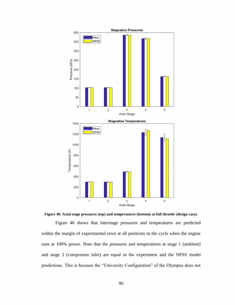
90
Figure 40. Axial stage pressures (top) and temperatures (bottom) at full throttle (design case).
Figure 40 shows that interstage pressures and temperatures are predicted
within the margin of experimental error at all positions in the cycle when the engine
runs at 100% power. Note that the pressures and temperatures at stage 1 (ambient)
and stage 2 (compressor inlet) are equal in the experiment and the NPSS model
predictions. This is because the “University Configuration” of the Olympus does not

91
provide total pressure and temperature measurements at the compressor inlet, and it
was assumed that the flow conditions at the compressor inlet were simply equal to
ambient conditions. This is a reasonable assumption because typical diffuser
efficiencies are close to 1.0 [10]. For this reason, the diffuser/inlet efficiency in the
NPSS model was also assumed to be 1.0.
Uncertainties in T04 and T05 are relatively large (~ +/-70 K), due to the
uncertainties in the parameters used to make the thermocouple corrections (i.e., wall
emissivity, thermal conductivity, wall temperature, dynamic viscosity, etc.).
Figure 41 shows the percent difference between measured and predicted axial
stage stagnation pressures and temperatures at various throttle settings. Temperatures
are predicted within 5% at all throttle settings and pressure to within 2.5% except P03
and P04 at 20% throttle which are predicted to within about 9%.
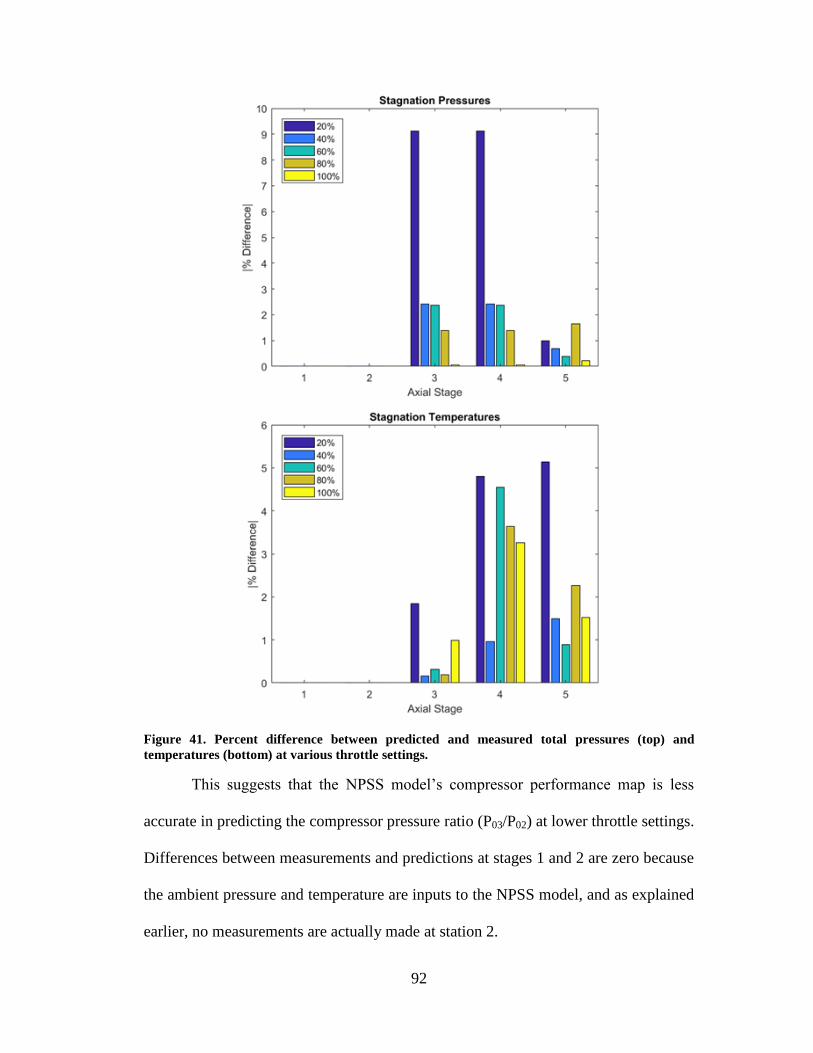
92
Figure 41. Percent difference between predicted and measured total pressures (top) and
temperatures (bottom) at various throttle settings.
This suggests that the NPSS model’s compressor performance map is less
accurate in predicting the compressor pressure ratio (P03/P02) at lower throttle settings.
Differences between measurements and predictions at stages 1 and 2 are zero because
the ambient pressure and temperature are inputs to the NPSS model, and as explained
earlier, no measurements are actually made at station 2.

93
5.2.2 Thrust, Fuel Flow Rate, & TSFC Comparison
Figure 42 compares the measured and predicted thrust as functions of
corrected RPM (defined in “Appendix A: Compressor & Turbine Performance
Maps”) and throttle setting.
Figure 42. Thrust as a function of corrected RPM (top) and throttle setting (bottom).

94
Recall that measured thrust is a dependent condition for the NPSS solver
during on- and off-design analysis. During off-design cases, the solver adjusts certain
independents (which include RPM) such that the calculated thrust equals the
measured thrust at each throttle setting (see Section “3.3.2 Independents and
Dependents”). Because the exhaust static pressure (Ps6) is not measured, NPSS cannot
predict exhaust velocity (and thus thrust) directly from the measured interstage
pressures and temperatures. Although the measured and NPSS thrust values are equal
at each throttle setting (bottom plot of Figure 42), they are offset from each other
when plotted against corrected RPM (top plot of Figure 42). This is due to the
difference between measured and predicted corrected RPM at each throttle setting
(see Figure 43).
Figure 43. Comparison between measured and predicted corrected RPM.
The corrected RPM values are equal at full throttle because this was the
design point for the NPSS model, and the NPSS solver does not adjust RPM in design

95
mode. The offset in RPM may be due to the inaccuracy of the turbomachinery maps
used to predict compressor and turbine performance.
Similarly, the measured fuel flow rate is an input to the NPSS model, so the
experimental values equal the model values. The same offset in corrected RPM
observed with thrust is also observed when comparing fuel flow rate values (see
Figure 44).
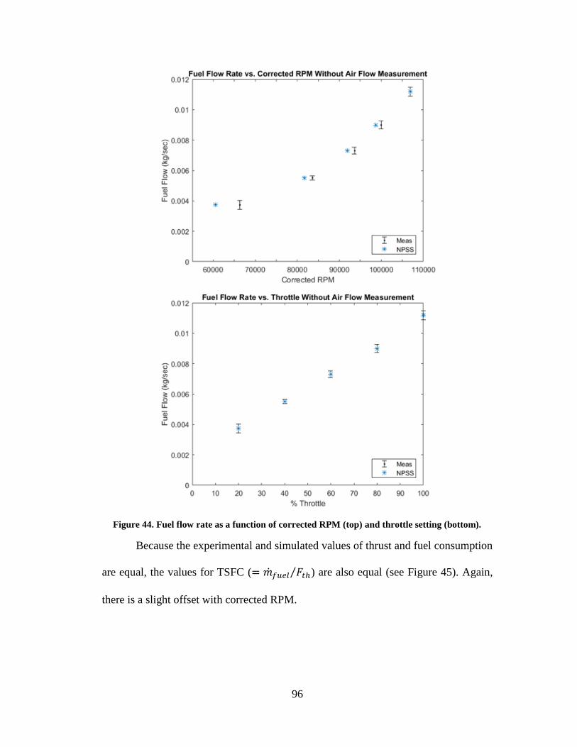
96
Figure 44. Fuel flow rate as a function of corrected RPM (top) and throttle setting (bottom).
Because the experimental and simulated values of thrust and fuel consumption
are equal, the values for TSFC ( ) are also equal (see Figure 45). Again,
there is a slight offset with corrected RPM.
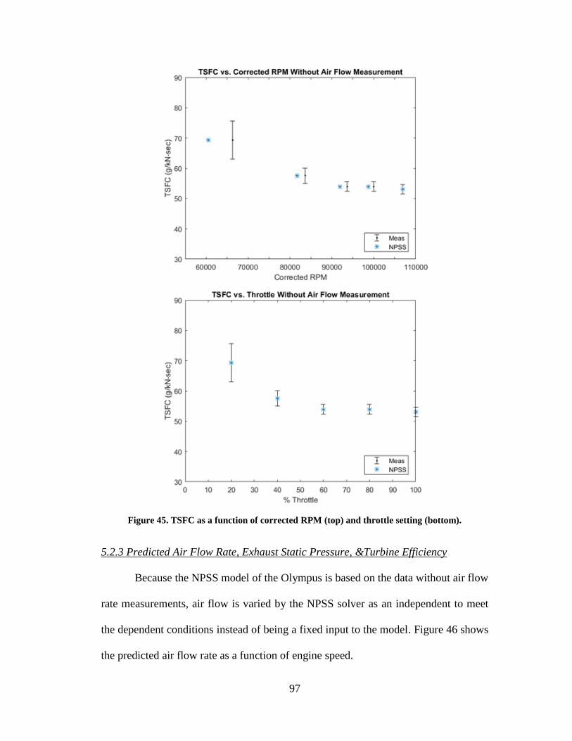
97
Figure 45. TSFC as a function of corrected RPM (top) and throttle setting (bottom).
5.2.3 Predicted Air Flow Rate, Exhaust Static Pressure, &Turbine Efficiency
Because the NPSS model of the Olympus is based on the data without air flow
rate measurements, air flow is varied by the NPSS solver as an independent to meet
the dependent conditions instead of being a fixed input to the model. Figure 46 shows
the predicted air flow rate as a function of engine speed.
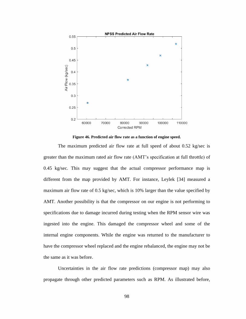
98
Figure 46. Predicted air flow rate as a function of engine speed.
The maximum predicted air flow rate at full speed of about 0.52 kg/sec is
greater than the maximum rated air flow rate (AMT’s specification at full throttle) of
0.45 kg/sec. This may suggest that the actual compressor performance map is
different from the map provided by AMT. For instance, Leylek [34] measured a
maximum air flow rate of 0.5 kg/sec, which is 10% larger than the value specified by
AMT. Another possibility is that the compressor on our engine is not performing to
specifications due to damage incurred during testing when the RPM sensor wire was
ingested into the engine. This damaged the compressor wheel and some of the
internal engine components. While the engine was returned to the manufacturer to
have the compressor wheel replaced and the engine rebalanced, the engine may not be
the same as it was before.
Uncertainties in the air flow rate predictions (compressor map) may also
propagate through other predicted parameters such as RPM. As illustrated before,

99
NPSS predictions for RPM are outside of the experimental margin of error. Resolving
the issues with the current method of measuring air flow rate will allow a compressor
map to be determined experimentally. Replacing the map provided by AMT in the
current NPSS model with an experimentally determined compressor performance
map should reduce the uncertainty in the predicted air flow rate and reduce error
propagation to other predicted parameters.
Exhaust static pressure (not measured) is also varied by the NPSS solver to
meet the dependent conditions. Figure 47 shows the predicted Ps6 as a function of
engine speed.
Figure 47. Predicted exhaust static pressure as a function of engine speed.
At higher engine speeds (40% – 100% throttle), NPSS predicts Ps6 to be
greater than ambient pressure (~100 kPa). This may make physical sense when
considering the performance of the exhaust ejector. As mentioned previously, the
fume hood attached to the exhaust ejector cannot keep up with the engine’s exhaust at

100
speeds greater than about 40% throttle. The fume hood’s inability to engulf the
engine’s exhaust will presumably create backpressure behind the nozzle. Since the
Olympus in “University Configuration” does not provide a Ps6 measurement port, a
method of making this measurement to confirm the NPSS predicted values still needs
to be developed.
Another parameter adjusted by the NPSS solver is turbine efficiency which is
depicted in Figure 48.
Figure 48. Predicted turbine efficiency as a function of engine speed.
There appears to be a slight increase in turbine efficiency as the engine speed
increases. The minimum turbine efficiency of 0.683 occurs at about 60,000 corrected
RPM, and the maximum turbine efficiency of 0.692 occurs at about 107,000
corrected RPM. Recall that turbine performance is predicted using a scaled low
pressure turbine map from GE. There is some uncertainty associated with scaling a
turbine map from a larger engine to the size required for a smaller engine. This

101
uncertainty will certainly affect predicted turbine efficiency and other predicted
parameters (such as RPM). As with the current compressor map, the GE turbine map
could be replaced with an experimentally determined performance map once the
issues with the air flow rate measurements are resolved.
5.2.4 Thrust with & without Air Flow Rate Measurement
As discussed previously, the air flow rate measurement apparatus reduces the
freestream pressure significantly. While this should reduce the thrust produced by the
engine, the measurements indicate that this not the case (see Figure 49). This
apparently non-physical result suggests that the air flow measurement may be
corrupting the thrust measurement.
Figure 49. Thrust comparison for the case with and without the air flow rate measurement.
Figure 49 shows that the measured thrust is significantly larger when air flow
rate is measured compared to when it is not despite the larger inlet pressure losses
when the air flow rate measurement apparatus is installed.

102
One possible explanation is that this discrepancy is caused by the difference in
pressure between the lab and the air plenum. Air in the lab (which is at a greater
pressure than that inside the plenum) pushes on the flexible rubber diaphragm forcing
it inward toward the plenum. Since the diaphragm is connected to the inlet extension
which, in turn, is connected to the thrust stand, this force may be transmitted to the
thrust stand in a way that adds to the thrust of the engine. Resolving this problem will
require a complete re-design of the air inlet and plenum. The apparently non-physical
thrust measurements associated with the air flow rate measurements are the reason
that the current NPSS model has been developed based on the experimental data
without air flow rate measurements.
A remedy for this phenomenon would be to replace the LFE-plenum-duct
configuration with a bell mouth diffuser that is attached directly to the engine’s inlet.
This would prevent the need for a diaphragm or any type of rigid attachment of the air
flow rate measurement device to the tabletop. At the time of writing this thesis, AMT
developed a bell mouth diffuser (or ‘extended intake’) designed specifically to
measure air flow rate for the Olympus engine. A schematic diagram of the Olympus
engine with the extended diffuser is provided in Figure 50, and a picture of the
Olympus with the diffuser attached is provided in Figure 51.

103
Figure 50. Schematic diagram of the Olympus engine in “University Configuration” with the
extended intake [21].
Figure 51. Olympus engine with the extended intake attached to the inlet [21].
When designing the test facility, the LFE was the preferred method of air flow
rate measurement because it was a pre-fabricated and pre-calibrated instrument with
high accuracy. Unfortunately, there were unforeseen complications with attaching the
LFE to the engine without disrupting the thrust measurements. Also, the extended
intake for measuring air flow rate for the Olympus was not yet available from AMT.

104
Chapter 6: Conclusions & Future Work
6.1 Summary & Key Findings
This thesis has developed an experimentally validated thermodynamic model
of a small gas turbine engine (AMT Olympus) that will be used as platform for
constructing a bench-scale hybrid GT/SOFC system. The thermodynamic model of
the engine was created using an industry standard software tool called Numerical
Propulsion System Simulation (NPSS). The model uses a compressor map supplied
by AMT and a scaled version of one of General Electric’s low pressure turbine maps
for the turbine. An indoor test facility was constructed to measure the engine’s
performance. Measurements include axial stage stagnation temperatures and
pressures, thrust, fuel flow rate, air flow rate, and engine speed (RPM). Measured
turbine inlet (T04) and turbine exit (T05) temperatures are corrected for conduction and
radiation losses in the thermocouples. The NPSS model is validated by comparing
predicted and experimentally measured performance parameters as functions of
engine speed (or throttle setting) for steady state engine operation.
The key findings of this work are summarized below:
Interstage pressures are predicted to within 2.5% of the measurements
with the exception of P03 and P04 at 20% throttle which are predicted to
within 9%
Interstage temperatures are predicted to within 5% of the measurements
Predicted air flow rate, exhaust static pressure, and turbine efficiency
o The maximum NPSS predicted air flow rate is greater than the
maximum rated air flow rate (specified by AMT) which could be

105
due to a change in compressor performance after replacing the
original compressor or an inaccuracy in the compressor map
provided by AMT
o Ps6 is greater than ambient pressure at higher engine speeds which
is likely due to the exhaust ejector’s failure to engulf all of the
engine’s exhaust at these speeds
o Turbine efficiency does not appear to be a strong function of
engine speed, reaching a minimum of 0.683 at about 60,000
corrected RPM and a maximum of 0.692 at about 107,000
corrected RPM
6.2 Contributions
This work presents two major contributions to modeling and performance
testing of small gas turbine engines (particularly the AMT Olympus):
1. Developed an indoor small gas turbine (< 445 N) test facility that measures
all global performance parameters (thrust, air flow rate, fuel flow rate, engine
speed (RPM), and axial stage stagnation temperatures and pressures)
2. Developed what is believed to be the first Numerical Propulsion System
Simulation (NPSS) thermodynamic model of the AMT Olympus gas turbine
engine and validated it via comparison to experimental data
6.3 Future Work
Suggested improvements to this work and the next steps toward achieving a
functional GT/SOFC prototype are outlined below:

106
Replace the LFE-plenum-duct configuration for measuring air flow rate with
the extended intake manufactured by AMT to avoid disrupting the thrust
measurements
o Use air flow measurements to create compressor and turbine
performance maps based on experimental measurements
o Replace current turbomachinery maps in NPSS model with the
experimentally determined maps
Replace the MDF tabletop with a more rigid surface such as an optical table
breadboard with threaded holes to maintain a rigid contact point between the
thrust stand and load cell
Measure static pressure at the nozzle exit during engine runs
o Better understand how the presence of the exhaust ejector affects
thrust measurements
o Enables thrust prediction from interstage measurements
Have fuel samples tested to determine a more accurate lower heating value of
combustion to be input into the NPSS burner model
Perform a sensitivity analysis to examine how certain input parameters (such
as compressor/turbine maps) affect NPSS calculations
o The current NPSS model predictions are sensitive to the uncertainties
in the turbomachinery maps (i.e., air flow rate, turbine efficiency, etc.),
affecting the ability to make meaningful comparisons to measurements

107
Develop an NPSS model of a commercially available SOFC system, and
integrate this model into the existing model of the AMT Olympus to design
the hybrid prototype system
o A colleague is currently working toward this aim using the developed
NPSS model of the Olympus engine presented in this work

108
Appendix A: Compressor & Turbine Performance Maps
A.1 Olympus Compressor Map
The compressor map for the Olympus was provided directly from AMT.
Figure 52. AMT Olympus compressor performance map.
The corrected air mass flow rate is defined in Eq. (58):
(58)
where is the temperature correction factor, is the pressure correction factor,
is the reference pressure ( = 100 kPa), and is the reference temperature (
= 298 K). The corrected shaft speed is defined in Eq. (59):
(59)
where is again the temperature correction factor.

109
A.2 Low Pressure Turbine Map
The low pressure turbine map below is the unscaled version of the
performance map used in the Olympus engine model. It was created by General
Electric as part of NASA’s Energy Efficient Engine (E3) program [81] and included
in the NPSS software package [76]. The corrected mass flow and shaft speed are
defined here the same as in Appendix “A.1 Olympus Compressor Map”.
Figure 53. General Electric's low pressure turbine performance map from the Energy Efficient
Engine Program [1].

110
Appendix B: Details of NPSS Olympus Model
B.1 Order of Execution
In a physical gas turbine system, the flow properties at a particular stage in the
engine depend on the flow properties further upstream of that stage. Similarly, the
components in an NPSS engine model rely on flow information stored and passed
from preceding elements to calculate performance of the current element. Elements
must be ordered such that the current element receives all required flow information
to calculate its own flow properties and propagate that information downstream.
Below is the order in which elements are executed for this work:
1. Ambient element: AmbientNASA ‘Amb’
2. Inlet Start element: InletStartNASA ‘InletStart’
3. Inlet element: Inlet ‘InEng’
4. Compressor element: Compressor ‘CmpH’
5. Fuel Start element: FuelStart ‘FusEng’
6. Burner element: Burner ‘BrnPri’
7. Turbine element: Turbine ‘TrbH’
8. Duct element: DuctNASA ‘D043’
9. Nozzle element: NozzleNASA ‘NozPri’
10. Flow End element: FlowEnd ‘FePri’
11. Shaft element: Shaft ‘ShH’

111
B.2 How to Run an NPSS Model
Below is an extremely basic outline on how to run an NPSS model:
1. Define an engine model (‘.mdl’) file.
a. Include all necessary components (elements), and declare them in
proper order.
b. Be sure all fluid and shaft ports are linked properly.
c. Input parameters for each element may be declared in this file, but
they are typically changed in the ‘.case’ file.
2. Define a case (‘.case’) file.
a. Define a design case to set the baseline engine model according to
specified design parameters.
b. Define one or more off-design cases that adjust the model’s input
parameters to find operating conditions away from the design point.
c. Make sure the solver is configured with the same number of
independents as dependents for each case.
3. Define a run (‘.run’) file.
a. The desired thermodynamics package is usually declared here.
b. Include any output files, the model file, and the case file.
c. The order in which files are included is important. For example, if the
case file calls an output file, the output file should be included before
the case file. Similarly, make sure the case file is included after the
model file so that input parameters are initialized and changed
properly.

112
4. Run the model.
a. Open the NPSS command line prompt. To run the model, use the
command “npss.nt RunFileName.run”. Be sure to include the file name
extension ‘.run’.
b. Make sure the NPSS command line prompt is in the same
path/directory as all relevant files (‘.run’, ‘.case’, ‘.mdl’ files, etc.).

113
Appendix C: Example NPSS Code
C.1 Turbojet ‘.run’ Run File
The following code is used to setup and run a turbojet engine model in NPSS.
It declares the thermodynamics package and includes all relevant files such as output
files, the model file, and case files.
Contents of the ‘.run’ file:
//Set the thermo package
setThermoPackage("CEA", "Air", "H2O", "Jet-A(L)", "O2", "H2", "H",
"O", "N", "C", "Ar" );
//output files
#include "Viewers/perf_Olympus.view"
#include "Viewers/stage_Olympus.view"
//model file
// #include "turbojet.mdl"
#include "olympusNASAIn.mdl"
setOption("switchTransport","EQUIL");
//set parameters
#include "Parameters/solver_var.int" //solver independents and
//dependents
//case input files
// #include "turbojet.case"
#include "Cases/olympusNASAIn.case"
// #include "Cases/SensitivityOD.case"
// #include "Cases/SensitivityDes.case"
//convergence statistics
// #include "ConvergeStats.report"

114
C.2 Example ‘.case’ Case File
The following code defines multiple cases to be run with the engine model. It
runs a design case where the baseline engine model is set followed by several off-
design cases that predict engine performance away from the design point.
Contents of the ‘.case’ file:
// conversion factors
real kelv_to_rank = 9./5;
real rank_to_kelv = 5./9;
perfTitles(); //set up headings in perf output file
stageTitles(); //set up headings in stage output file
setOption( "switchDes", "DESIGN" );
autoSolverSetup();
solver.addIndependent( "AirControl" );
// solver.addIndependent( "TurbPR" );
// solver.addIndependent( "TurbEff" );
// solver.addIndependent( "Qloss" );
// solver.addDependent( "Thrust" );
solver.addDependent( "TIT" );
// solver.removeIndependent( "TrbH.S_map.ind_parmMap");
cout << "\n\nDesign independents:\n" << solver.independentNames;
cout << "\n\nDesign Dependents:\n" << solver.dependentNames;
//based on initial experimental data (max RPM case)
Amb.switchMode = "PSTSMN";
Amb.Ps_in = 14.523;
Amb.Ts_in = 535.05; //297.25K
CmpH.S_map.PRdes = 3.7;
CmpH.S_map.effDes= 0.75;
BrnPri.dPqPBase = 1-0.948;
BrnPri.Wfuel = 0.0262;
BrnPri.Qhx = 116.857;
TrbH.S_map.effDes = 0.729166;
NozPri.PsExh = Amb.Ps_in;
real throttle;
throttle = 100.;
int HoodOn;
HoodOn = 0;
TIT_max = 1200.*kelv_to_rank;
Fn_target = 52.6; // from AMT data @ max RPM
// BrnPri.Fl_O.setOption("switchPrint", "TRUE");
BrnPri.Fl_O.A = 19.729; // combustor area, in^2

115
TrbH.Fl_O.A = 5.69; // turbine exit area, in^2
run();
perfPrint();
stagePrint();
setOption( "switchDes", "OFFDESIGN" );
autoSolverSetup();
// cout << "\n\nDesign independents:\n" << solver.independentNames;
// cout << "\n\nDesign Dependents:\n" << solver.dependentNames;
run();
perfPrint();
real Fn_FT = Perf.Fn; //initial full throttle thrust
solver.addIndependent( "Qloss" );
// solver.addIndependent( "TurbPR" );
// solver.addIndependent( "TurbEff" );
solver.addDependent( "Thrust" );
// solver.addDependent( "TIT" );
solver.maxIterations = 100;
solver.maxJacobians = 100;
cout << "\n\nOff-Design independents:\n" << solver.independentNames;
cout << "\n\nOff-Design Dependents:\n" << solver.dependentNames;
real throt[] = {23.5,38.89,51.28,61.54,71.37,79.91,
87.61,94.02,100.};
real TambK[] = {295.79,295.72,295.94,296.62,296.78,296.09,
296.98,296.90,297.25};
real Pamb[] = {14.632,14.606,14.581,14.564,14.554,14.542,
14.533,14.530,14.523};
real fuel[] = {0.009000,0.011466,0.013655,0.015781,0.017847,
0.020004,0.022069,0.024319,0.0262};
real fuelEff[] = {0.925549495,0.925138808,0.927036074,0.928615835,
0.928850157,0.935733732,0.940858224,0.941247835,0.947688425};
int i;
for(i=0;i<throt.entries();i++) {
throttle = throt[i];
Amb.Ts_in = TambK[i]*kelv_to_rank;
Amb.Ps_in = Pamb[i];
Fn_target = throt[i]/100.*Fn_FT;
BrnPri.Wfuel = fuel[i];
BrnPri.dPqPBase = 1-fuelEff[i];
NozPri.PsExh = Pamb[i];
HoodOn = 0;
run();
perfPrint();
stagePrint();
}

116
C.3 Turbojet ‘.mdl’ Model File
The following code declares the gas turbine components that define the engine
model.
Contents of the ‘.mdl’ file:
Element AmbientNASA Amb {
switchMode = "ALDTMN";
alt_in = 0.;
dTs_in = 0.;
MN_in = 0.;
} //END Amb
Element InletStartNASA InletStart{
AmbientName = "Amb";
W_in = 0.99; // max flow rate
} //END InletStart
Element Inlet InEng {
eRamBase = 1.0;
} //END InEng
Element Compressor CmpH {
#include "Maps/olympusCompEff.map";
S_map.PRdes = 3.8;
S_map.effDes= 0.719;
S_map.RlineMap = 1.3;
S_map.NcDes = 1.0;
} //END CmpH
Element FuelStart FusEng {
fuelType = "Jet-A(L)"; // define fuel type for CEA
hFuel = -779.584;
} //END FusEng
Element Burner BrnPri {
dPqPBase = 0.05;
effBase = 0.95;
Qhx = 115.;
switchBurn = "FUEL";
Wfuel = 0.0235; // fuel flow @ max RPM
tolRayleigh = 0.0001;
} //END BrnPri
Element Turbine TrbH {
#include "Maps/lptE3.map"; //low pressure turbine map
S_map.parmMapDes = 2.098;

117
S_map.parmNcDes = 100.0;
S_map.effDes = 0.80;
// eff = 0.80;
// PRbase = 2.265;
} //END TrbH
Element DuctNASA D043 {
switchDP = "INPUT";
void preexecute() {
dPqP_in = 0.25 * Fl_I.MN * Fl_I.MN;
}
Fl_I.MNdes = 0.4;
} //END D043
Element NozzleNASA NozPri {
// PsExhName = "Amb.Ps";
PsExh = 14.7;
setOption("switchFrozen","EQUIL");
} //END NozPri
Element FlowEnd FePri {
} //END FePri
Element Shaft ShH {
// Mechanical Ports. These are created as needed on the shaft.
ShaftInputPort MeCmpH, MeTrbH;
Nmech = 108500.; // max shaft speed (design point)
} //END ShH
Element PerfNASA Perf {
} //END Perf
// -------------------------------
// linkPorts
// -------------------------------
linkPorts( "InletStart.Fl_O", "InEng.Fl_I", "F_1" );
linkPorts( "InEng.Fl_O", "CmpH.Fl_I", "F_2" );
linkPorts("CmpH.Fl_O", "BrnPri.Fl_I", "F_3" );
linkPorts( "FusEng.Fu_O", "BrnPri.Fu_I", "F_4" );
linkPorts( "BrnPri.Fl_O", "TrbH.Fl_I", "F_5" );
linkPorts( "TrbH.Fl_O", "D043.Fl_I", "F_6" );
linkPorts( "D043.Fl_O", "NozPri.Fl_I", "F_7" );
linkPorts( "NozPri.Fl_O", "FePri.Fl_I", "F_8" );
// -------------------------------
// Shaft Connect Statements
// -------------------------------
linkPorts( "CmpH.Sh_O", "ShH.MeCmpH", "MeCmpH" );
linkPorts( "TrbH.Sh_O", "ShH.MeTrbH", "MeTrbH" );

118
Appendix D: Experimental Data
D.1 Performance Data without Air Flow Rate Measurements
These data are averaged over five runs at each throttle setting. The values of
T04 and T05 are corrected for conduction and radiation losses in the thermocouples.
This data set was used to generate the results reported in this work.
% Throttle 20 40 60 80 100
RPMc 66329.76 83642.83 93676.76 99979.95 106957.6
Thrust (N) 53.84159 95.68119 135.4801 166.6891 210.7888
Fuel Flow (kg/s) 0.00373 0.00551 0.007304 0.00899 0.011188
TSFC (g/kN-s) 69.30894 57.60343 53.92097 53.93981 53.08401
Pamb (kPa) 102.1944 102.1606 102.1403 102.1267 101.9709
P03 (kPa) 187.1453 253.0807 306.2492 342.3898 385.5344
P04 (kPa) 172.5758 235.4037 287.1719 323.2899 366.9106
P05 (kPa) 110.2941 124.4936 136.7637 146.5123 162.5681
Tamb (K) 294.8709 294.7877 295.1041 295.8127 296.5325
T03 (K) 362.9853 405.2246 436.1717 458.1209 489.8702
T04 (K) 945.121 974.0879 1030.479 1125.402 1228.329
T05 (K) 892.1089 876.0026 951.07 1009.646 1132.441

119
D.2 Performance Data with Air Flow Rate Measurements
These data are averaged over five runs at each throttle setting. The values of
T04 and T05 are corrected for conduction and radiation losses in the thermocouples.
% Throttle 20 40 60 80 100
RPMc 65915.48 84208.1 93815.04 100507.9 107298.7
Thrust (N) 90.13677 153.7327 200.5396 240.282 282.8758
Air Flow (kg/sec) 0.227815 0.317627 0.364099 0.39163 0.40518
Fuel Flow (kg/s) 0.003922 0.005631 0.007314 0.009081 0.011304
TSFC (g/kN-s) 43.52936 36.63897 36.48742 37.80207 39.9616
Pamb (kPa) 101.6594 101.6526 101.6323 101.6255 101.6255
P02 (kPa) 96.02101 94.35704 93.37997 92.73244 92.16315
P03 (kPa) 181.79 250.572 300.5491 339.1346 379.5129
P04 (kPa) 168.041 233.6222 282.0071 320.1258 361.7134
P05 (kPa) 109.39 124.4237 135.7178 146.0545 161.796
Tamb (K) 294.1606 293.5967 293.6114 293.8666 294.6387
T03 (K) 361.7471 406.0616 435.299 458.5792 487.8886
T04 (K) 974.7461 990.0407 1037.99 1140.946 1247.238
T05 (K) 934.7274 881.9539 950.8339 1029.453 1132.759

120
Bibliography
[1] D. F. Waters, “Modeling of Gas Turbine - Solid Oxide Fuel Cell Systems for
Combined Propulsion and Power on Aircraft.,” University of Maryland,
College Park, 2015.
[2] A. T. Isikveren, “Future of [More] Electrical Aircraft,” ICAS Biennial
Workshop. Cape Town, South Africa, 2013.
[3] S. W. Ashcraft, A. S. Padron, K. A. Pascioni, G. W. Stout, and D. L. Huff,
“Review of Propulsion Technologies for N+3 Subsonic Vehicle Concepts,”
NASA/TM-2011-217239. 2011.
[4] P. Jackson, K. Munson, and L. Peacock, IHS Jane’s All the World’s Aircraft:
Development & Production. Alexandria, VA: IHS Global, Inc., 2014.
[5] M. Daly and M. Streetly, IHS Jane’s All the World’s Aircraft: Unmanned.
Alexandria, VA: IHS Global, Inc., 2015.
[6] A. Choudhury, H. Chandra, and A. Arora, “Application of solid oxide fuel cell
technology for power generation - A review,” Renewable and Sustainable
Energy Reviews, vol. 20. pp. 430–442, 2013.
[7] K. Rajashekara, J. Grieve, and D. Daggett, “Solid oxide fuel cell/gas turbine
hybrid APU system for aerospace applications,” in IEEE Industry Applications
Conference, 2006, pp. 2185–2192.
[8] J. Islas, “The Gas Turbine:: A New Technological Paradigm in Electricity
Generation,” Technol. Forecast. Soc. Change, vol. 60, pp. 129–148, 1999.
[9] M. Hepperle, “Electric Flight - Potential and Limitations,” NATO,
Braunschweig, Germany.
[10] P. G. Hill and C. R. Peterson, Mechanics and Thermodynamics of Propulsion,
2nd ed. Reading, MA: Addison-Wesley, 1992.
[11] T. Lombardo, “Inside Siemens’ Record-Breaking Electric Aircraft Motor,”
2016. [Online]. Available:
http://www.engineering.com/ElectronicsDesign/ElectronicsDesignArticles/Arti
cleID/12805/Inside-Siemens-Record-Breaking-Electric-Aircraft-Motor.aspx.
[Accessed: 21-Sep-2016].
[12] Aviation Week Network, “Jet-A and Avgas Fuel Prices: August 2015.”
[Online]. Available: http://aviationweek.com/%5Bprimary-term%5D/jet-and-
avgas-fuel-prices-august-2015. [Accessed: 21-Sep-2016].
[13] M. K. Bradley and C. K. Droney, “Subsonic Ultra Green Aircraft Research:
Phase II – Volume II – Hybrid Electric Design Exploration,” NASA/CR–2015-
218704, vol. 2, 2015.

121
[14] Northrop Grumman, “Targets Fact Sheet.” [Online]. Available:
http://www.northropgrumman.com/Capabilities/BQM74EAerialTarget/Docum
ents/TGTS-Fact-Sheet.pdf. [Accessed: 05-Sep-2016].
[15] J. D. Mattingly, Elements of Propulsion: Gas Turbines and Rockets. Reston,
VA: AIAA, 2006.
[16] M. J. Moran and H. N. Shapiro, Fundamentals of Engineering
Thermodynamics, 6th ed. Hoboken, NJ: John Wiley & Sons, Inc., 2008.
[17] R. D. Flack, Fundamentals of Jet Propulsion with Applications. NY:
Cambridge University Press, 2005.
[18] PBS Aerospace, “Turbojet Engines.” [Online]. Available:
http://www.pbsaerospace.com/engines/turbojet-engines. [Accessed: 05-Sep-
2016].
[19] PBS Aerospace, “TJ 100 Turbojet Engine.” [Online]. Available:
http://www.pbsaerospace.com/our-products/tj-100-turbojet-engine. [Accessed:
05-Sep-2016].
[20] Sonex, “SubSonex: The Personal Jet Reality Check.” [Online]. Available:
http://www.sonexaircraft.com/subsonex/index.html. [Accessed: 05-Sep-2016].
[21] AMT Netherlands, “Products.” [Online]. Available:
http://www.amtjets.com/pdf/University-Olympus-HP-Jan-2017.pdf.
[22] Jetman Dubai, “Homepage.” [Online]. Available: http://www.jetman.com/.
[Accessed: 05-Sep-2016].
[23] E. Benini and S. Giacometti, “Design, manufacturing and operation of a small
turbojet-engine for research purposes,” Appl. Energy, vol. 84, no. 11, pp.
1102–1116, 2007.
[24] A. J. B. Jackson, P. Laskaridis, and P. Pilidis, “A test bed for small aero gas
turbines for education and for university - Industry collaboration,” in
Proceedings of the ASME Turbo Expo 2004, 2004, pp. 901–909.
[25] C. R. Davison and A. M. Birk, “Set Up and Operational Experience With a
Micro-Turbine Engine for Research and Education,” in Proceedings of the
ASME Turbo Expo 2004, 2004, pp. 849–858.
[26] Turbine Technologies, “MiniLab: Gas Turbine Power System.” [Online].
Available:
http://www.turbinetechnologies.com/Portals/0/pdfs/specifications/minilab
Specs.pdf. [Accessed: 05-Sep-2016].
[27] M. Badami, P. Nuccio, and A. Signoretto, “Experimental and numerical
analysis of a small-scale turbojet engine,” Energy Convers. Manag., vol. 76,
pp. 225–233, 2013.

122
[28] AMT Netherlands, “Olympus HP in University Configuration: Spec Sheet.”
[Online]. Available: http://www.amtjets.com/pdf/University-Olympus-HP-Jan-
2013.pdf.
[29] A. Al-Alshaikh, “An Experimental and Numerical Investigation of the Effect
of Aero Gas Turbine Test Facility Aspect Ratio on Thrust Measurement,”
Cranfield University, 2011.
[30] D. P. Bakalis and A. G. Stamatis, “Data analysis and performance model
calibration of a small turbojet engine,” in Proceedings of the Institution of
Mechanical Engineers, 2011, pp. 1523–1533.
[31] R. GRZESZCZYK, J. MERKISZ, M. GÓRECKI, B. van de GOOR, and E.
KAMIŃSKA, “The Laboratory Test Bench for a Small Turbojet Engine.”
2011.
[32] A. Horoufi and M. Boroomand, “Design and Construction of Microjet
Engine,” in 45th AIAA/ASME/SAE/ASEE Joint Propulsion Conference &
Exhibit, 2009.
[33] P. Laskaridis, P. Pilidis, and V. Pachidis, “Small Scale Engine Test Bed Design
and Optimisation,” in Design Optimization International Conference, 2004.
[34] Z. Leylek, “An Investigation into Performance Modelling of a Small Gas
Turbine Engine,” Australia, 2012.
[35] N. U. Rahman and J. F. Whidborne, “A numerical investigation into the effect
of engine bleed on performance of a single-spool turbojet engine,” in
Proceedings of the Institution of Mechanical Engineers, 2008, pp. 939–949.
[36] R. O’Hayre, S. Cha, W. Colella, and F. B. Prinz, Fuel Cell Fundamentals, 2nd
ed. Hoboken, NJ: John Wiley & Sons, Inc., 2009.
[37] X. Li, Principles of Fuel Cells. New York: Taylor & Francis Group, 2006.
[38] R. J. Kee, H. Zhu, and G. S. Jackson, “Solid Oxide Fuel Cells Using Syngas,”
in Synthesis Gas Combustion: Fundamentals and Applications, T. C. Lieuwen,
V. Yang, and R. Yetter, Eds. London: Taylor & Francis, 2009.
[39] Ballard Power Systems, “Products.” [Online]. Available:
http://www.ballard.com. [Accessed: 07-Sep-2016].
[40] B. C. H. Steele and A. Heinzel, “Materials for fuel-cell technologies,” Nature,
vol. 414, pp. 345–352, 2001.
[41] Y. Peng and J. T. Richardson, “Properties of ceramic foam catalyst supports:
one-dimensional and two-dimensional heat transfer correlations,” Appl. Catal.
A Gen., vol. 266, pp. 235–244, 2004.
[42] J. T. Richardson, D. Remue, and J.-K. Hung, “Properties of ceramic foam

123
catalyst supports: mass and heat transfer,” Appl. Catal. A Gen., vol. 250, pp.
319–329, 2003.
[43] L. D. Schmidt, E. J. Klein, C. A. Leclerc, J. J. Krummenacher, and K. N. West,
“Production of syngas by direct catalytic-oxidation of methane,” Chem. Eng.
Sci., vol. 58, p. 1037, 2003.
[44] J. T. Richardson, Y. Peng, and D. Remue, “Properties of ceramic foam catalyst
supports: pressure drop,” Appl. Catal. A Gen., vol. 204, pp. 19–32, 2000.
[45] K. E. Swider-Lyons, J. A. Mackrell, J. A. Rodgers, G. S. Page, M. W.
Schuette, and R. O. Stroman, “Hydrogen Fuel Cell Propulsion for Long
Endurance Small UAVs,” in AIAA Naval Centennial of Flight Forum, 2011.
[46] K. E. Swider-Lyons, R. O. Stroman, J. A. Rodgers, D. Edwards, J. A.
Mackrell, M. W. Schuette, and G. S. Page, “Liquid Hydrogen Fuel System for
Small Unmanned Air Vehicles,” in 51st AIAA Aerospace Meeting including
the New Horizons Forum and Aerospace Exposition, 2013.
[47] Intelligent Energy, “Intelligent Energy Hydrogen Fuel Cells Significantly
Extend Drone Flight Time.” [Online]. Available: http://www.intelligent-
energy.com/news-and-events/company-news/2015/12/15/intelligent-energy-
hydrogen-fuel-cells-significantly-extend-drone-flight-time/. [Accessed: 07-
Sep-2016].
[48] Intelligent Energy, “Major Drone Manufacturer Snaps Up Intelligent Energy’s
Game-Changer for Drone Range (Flight Time).” [Online]. Available:
http://www.intelligent-energy.com/news-and-events/company-
news/2016/01/28/major-drone-manufacturer-snaps-up-intelligent-energys-
game-changer-for-drone-range-fight-time/. [Accessed: 07-Sep-2016].
[49] Boeing, “Boeing Successfully Flies Fuel Cell-Powered Airplane.” [Online].
Available:
http://www.boeing.com/aboutus/environment/environmental_report/_inc/flash-
2-1-2.html. [Accessed: 07-Sep-2016].
[50] D. F. Waters and C. P. Cadou, “Engine-integrated solid oxide fuel cells for
efficient electrical power generation on aircraft,” J. Power Sources, vol. 284,
pp. 588–605, 2015.
[51] F. Calise, M. Dentice d’ Accadia, L. Vanoli, and M. R. von Spakovsky,
“Single-level optimization of a hybrid SOFC-GT power plant,” J. Power
Sources, vol. 159, no. 2, pp. 1169–1185, 2006.
[52] Y. Haseli, I. Dincer, and G. F. Naterer, “Thermodynamic modeling of a gas
turbine cycle combined with a solid oxide fuel cell,” Int. J. Hydrogen Energy,
vol. 33, no. 20, pp. 5811–5822, 2008.
[53] A. Abbasi and Z. Jiang, “Multidisciplinary modeling and simulation of a fuel

124
cell/gas turbine hybrid power system,” in 2009 IEEE Power and Energy
Society General Meeting, PES ’09, 2009, pp. 1–7.
[54] S. H. Chan, H. K. Ho, and Y. Tian, “Modelling of simple hybrid solid oxide
fuel cell and gas turbine power plant,” J. Power Sources, vol. 109, no. 1, pp.
111–120, 2002.
[55] J. Palsson, A. Selimovic, and L. Sjunnesson, “Combined solid oxide fuel cell
and gas turbine systems for efficient power and heat generation,” J. Power
Sources, vol. 86, no. 1, pp. 442–448, 2000.
[56] P. Costamagna, L. Magistri, and A. F. Massardo, “Design and part-load
performance of a hybrid system based on a solid oxide fuel cell reactor and a
micro gas turbine,” J. Power Sources, vol. 96, no. 2, pp. 352–368, 2001.
[57] T.-H. Lim, R.-H. Song, D.-R. Shin, J.-I. Yang, H. Jung, I. C. Vinke, and S.-S.
Yang, “Operating characteristics of a 5 kW class anode-supported planar
SOFC stack for a fuel cell/gas turbine hybrid system,” Int. J. Hydrogen
Energy, vol. 33, pp. 1076–1083, 2008.
[58] T. Suther, A. S. Fung, M. Koksal, and F. Zabihian, “Effects of operating and
design parameters on the performance of a solid oxide fuel cell-gas turbine
system,” Int. J. Energy Res., vol. 35, pp. 616–632, 2011.
[59] Y. Zhao, J. Sadhukhan, A. Lanzini, N. Brandon, and N. Shah, “Optimal
integration strategies for a syngas fuelled SOFC and gas turbine hybrid,” J.
Power Sources, vol. 196, no. 22, pp. 9516–9527, 2011.
[60] L. Leto, C. Dispenza, A. Moreno, and A. Calabr, “Simulation model of a
molten carbonate fuel cell-microturbine hybrid system,” Appl. Therm. Eng.,
vol. 31, no. 6–7, pp. 1263–1271, 2011.
[61] S. E. Veyo, L. A. Shockling, J. T. Dederer, J. E. Gillett, and W. L. Lundberg,
“Tubular Solid Oxide Fuel Cell/Gas Turbine Hybrid Cycle Power Systems:
Status,” J. Eng. Gas Turbines Power, vol. 124, pp. 845–849, 2002.
[62] J. E. Freeh, J. W. Pratt, and J. Brouwer, “Development of a Solid-Oxide Fuel
Cell/Gas Turbine Hybrid System Model for Aerospace Applications,” Vol. 7
Turbo Expo 2004, no. May, pp. 371–379, 2004.
[63] C. J. Steffen Jr., J. E. Freeh, and L. M. Larosiliere, “Solid oxide fuel cell/gas
turbine hybrid cycle technology for auxiliary aerospace power,” Proc. ASME
Turbo Expo, vol. 5, no. April, pp. 253–260, 2005.
[64] J. E. Freeh, C. J. Steffen, and L. M. Larosiliere, “Off-Design Performance
Analysis of a Solid-Oxide Fuel Cell/Gas Turbine Hybrid for Auxiliary
Aerospace Power,” 3rd Int. Conf. Fuel Cell Sci. Eng. Technol., no. December,
pp. 265–272, 2005.
[65] S. Eelman, I. d. P. y. d. Poza, and T. Krieg, “Fuel Cell APU ’ s in Commercial

125
Aircraft – An Assessment of SOFC and PEMFC Concepts,” in 24Th
International Congress of the Aeronautical Sciences, 2004.
[66] K. Rajashekara, J. Grieve, and D. Daggett, “Hybrid Fuel Cell Power in
Aircraft,” IEEE Industry Applications Magazine, pp. 54–60, 2008.
[67] R. J. Braun, M. Gummalla, and J. Yamanis, “System Architectures for Solid
Oxide Fuel Cell-Based Auxiliary Power Units in Future Commercial Aircraft
Applications,” J. Fuel Cell Sci. Technol., vol. 6, no. August 2009, p. 31015,
2009.
[68] A. Himansu, J. E. Freeh, C. J. Steffen, R. T. Tornabene, and X. Y. J. Wang,
“Hybrid solid oxide fuel cell / Gas turbine system design for high altitude long
endurance aerospace missions,” in Proceedings of 4th International ASME
Conference on Fuel Cell Science, Engineering and Technology,
FUELCELL2006, 2006.
[69] P. Aguiar, D. J. L. Brett, and N. P. Brandon, “Solid oxide fuel cell/gas turbine
hybrid system analysis for high-altitude long-endurance unmanned aerial
vehicles,” Int. J. Hydrogen Energy, vol. 33, no. 23, pp. 7214–7223, 2008.
[70] M. K. Bradley and C. K. Droney, “Subsonic Ultra Green Aircraft Research:
Phase I Final Report,” NASA/CR- 2011-216847, 2011.
[71] M. K. Bradley and C. K. Droney, “Subsonic Ultra Green Aircraft Research
Phase II: N+4 Advanced Concept Development,” NASA/CR- 2012-217556,
2012.
[72] A. R. Knott and C. P. Cadou, “Development of a Small Gas Turbine Engine
Test Facility,” University of Maryland, College Park, 2014.
[73] JetCat USA, “Products.” [Online]. Available: http://www.jetcatusa.com/rc-
turbines/.
[74] Jet Central USA, “Turbines.” [Online]. Available:
http://www.jetcentralusa.com/.
[75] KingTech Turbines, “Turbines.” [Online]. Available:
http://www.kingtechturbines.com/eshop/.
[76] NASA, “NPSS user guide, software release 1.6.5.” 2008.
[77] NASA, “NPSS developer’s guide, software release 1.6.5.” 2008.
[78] B. McBride and S. Gordon, “Computer Program for Calculation of Complex
Chemical Equilibrium Compositions and Applications II. User’s Manual and
Program Description.” NASA, RP-1311-P2, 1996.
[79] N. Sissenwine, M. Dubin, and H. Wexler, “The U.S. Standard Atmosphere,
1962,” J. Geophys. Res., vol. 67, no. 9, pp. 3627–3630, 1962.

126
[80] P. Batterton, “Energy efficient engine program contributions to aircraft fuel
conservation,” in Aviation Fuel Conservation Symposium, 1984.
[81] C. Ciepluch, D. Davis, and D. Gray, “Results of NASA’s energy efficient
engine program,” J. Propuls., vol. 3, no. 6, pp. 560–568, 1987.
[82] C. T. Kelley, Solving Nonlinear Equations with Newton’s Method.
Philadelphia: Society for Industrial and Applied Mathematics, 2003.
[83] J. Ortega and W. Rheinboldt, Iterative Solution of Nonlinear Equations in
Several Variables. New York: Academic Press, 1970.
[84] C. T. Kelley, Iterative Methods for Linear and Nonlinear Equations.
Philadelphia: Society for Industrial and Applied Mathematics, 1995.
[85] A. G. Kehlenbeck, “Development of a Thrust Stand for a Miniature Jet
Engine,” University of Maryland, College Park.
[86] National Weather Service, “College Park Airport Weather.” [Online].
Available: http://w1.weather.gov/obhistory/KCGS.html.
[87] Omega, “Thermocouples: Using Thermocouples in Temperature
Measurement.” [Online]. Available:
http://www.omega.com/prodinfo/thermocouples.html. [Accessed: 27-Sep-
2016].
[88] A. F. Mills, Basic Heat & Mass Transfer, 2nd ed. Upper Saddle River, NJ:
Prentice Hall, Inc., 1999.
[89] F. P. Incropera and D. P. DeWitt, Introduction to Heat Transfer, 2nd ed. John
Wiley & Sons, Inc., 1990.
[90] S. P. Venkateshan, “Systematic errors in temperature measurement.” Indian
Institute of Technology Madras.
[91] A. Faghri, Y. Zhang, and J. Howell, Advanced Heat and Mass Transfer. Global
Digital Press, 2010.
[92] AMT Netherlands, “Olmypus HP Manual.” 2017.
[93] The American Society of Mechanical Engineers, “ASME PTC 19.1-2005: Test
Uncerrtainty.” ASME International, New York, 2005.