Embed Size (px)
Citation preview
ABSTRACT
Title of dissertation: TECHNIQUES FOR VIDEO SURVEILLANCE:AUTOMATIC VIDEO EDITINGAND TARGET TRACKING
Hazem El-Alfy, Doctor of Philosophy, 2009
Dissertation directed by: Professor Larry S. DavisDepartment of Computer Science
Typical video surveillance control rooms include a collection of monitors con-
nected to a large camera network, with many fewer operators than monitors. The
cameras are usually cycled through the monitors, with provisions for manual over-
ride to display a camera of interest. In addition, cameras are often provided with
pan, tilt and zoom capabilities to capture objects of interest. In this dissertation, we
develop novel ways to control the limited resources by focusing them into acquiring
and visualizing the critical information contained in the surveyed scenes.
First, we consider the problem of cropping surveillance videos. This process
chooses a trajectory that a small sub-window can take through the video, selecting
the most important parts of the video for display on a smaller monitor area. We
model the information content of the video simply, by whether the image changes
at each pixel. Then we show that we can find the globally optimal trajectory for a
cropping window by using a shortest path algorithm. In practice, we can speed up
this process without affecting the results, by stitching together trajectories computed

over short intervals. This also reduces system latency. We then show that we
can use a second shortest path formulation to find good cuts from one trajectory
to another, improving coverage of interesting events in the video. We describe
additional techniques to improve the quality and efficiency of the algorithm, and
show results on surveillance videos.
Second, we turn our attention to the problem of tracking multiple agents
moving amongst obstacles, using multiple cameras. Given an environment with
obstacles, and many people moving through it, we construct a separate narrow field
of view video for as many people as possible, by stitching together video segments
from multiple cameras over time. We employ a novel approach to assign cameras
to people as a function of time, with camera switches when needed. The problem is
modeled as a bipartite graph and the solution corresponds to a maximum matching.
As people move, the solution is efficiently updated by computing an augmenting
path rather than by solving for a new matching. This reduces computation time
by an order of magnitude. In addition, solving for the shortest augmenting path
minimizes the number of camera switches at each update. When not all people can
be covered by the available cameras, we cluster as many people as possible into small
groups, then assign cameras to groups using a minimum cost matching algorithm.
We test our method using numerous runs from different simulators.
Third, we relax the restriction of using fixed cameras in tracking agents. In
particular, we study the problem of maintaining a good view of an agent moving
amongst obstacles by a moving camera, possibly fixed to a pursuing robot. This
is known as a two-player pursuit evasion game. Using a mesh discretization of the

environment, we develop an algorithm that determines, given initial positions of
both pursuer and evader, if the evader can take any moving strategy to go out of
sight of the pursuer, and thus win the game. If it is decided that there is no winning
strategy for the evader, we also compute a pursuer’s trajectory that keeps the evader
within sight, for every trajectory that the evader can take. We study the effect of
varying the mesh size on both the efficiency and accuracy of our algorithm.
Finally, we show some earlier work that has been done in the domain of
anomaly detection. Based on modeling co-occurrence statistics of moving objects in
time and space, experiments are described on synthetic data, in which time intervals
and locations of unusual activity are identified.
TECHNIQUES FOR VIDEO SURVEILLANCE:AUTOMATIC VIDEO EDITING AND TARGET TRACKING
by
Hazem Mohamed El-Alfy
Dissertation submitted to the Faculty of the Graduate School of theUniversity of Maryland, College Park in partial fulfillment
of the requirements for the degree ofDoctor of Philosophy
2009
Advisory Committee:
Professor Larry S. Davis, ChairProfessor David W. JacobsProfessor James ReggiaProfessor Ramani DuraiswamiProfessor Eyad Abed

c© Copyright byHazem El-Alfy
2009

Acknowledgments
I begin by thanking and praising Allah, the first Teacher to mankind. I cannot
thank Him properly without acknowledging the many people who have contributed
in making my career in graduate school a successful experience.
In this regard, I would like to thank my advisor Professor Larry Davis for his
readiness to supervise me at a tense moment during my graduate career. His patience
and suggestions for interesting and challenging problems helped me overcome that
period quickly. Along the same lines, I would like to acknowledge Professor David
Jacobs for his willingness to join us in our research. His hints and comments have
only made this thesis possible.
Additional thanks are due to Professors Eyad Abed, James Reggia and Ramani
Duraiswami for agreeing to serve on my committee and for sparing enough time for
this cause during this busy summer semester.
Mentioning everyone by name in the limited space I have here is impossible.
Many of my colleagues, friends and other people I came to know have helped me
in some way or the other. In the few remaining lines, I wish to acknowledge in
particular the encouragement and prayers of my mother and my father. I also
appreciate my wife for acting responsibly and patiently during times of harshness
as well as times of ease. Finally, my children Omar and Mariam have been my great
joys. They gave my life a different meaning.
ii

Table of Contents
List of Figures v
1 Introduction 11.1 Motivation . . . . . . . . . . . . . . . . . . . . . . . . . . . . . . . . . 11.2 Dissertation Organization . . . . . . . . . . . . . . . . . . . . . . . . 31.3 Contributions . . . . . . . . . . . . . . . . . . . . . . . . . . . . . . . 5
2 Automatic Video Editing 72.1 Introduction . . . . . . . . . . . . . . . . . . . . . . . . . . . . . . . . 72.2 Related Work . . . . . . . . . . . . . . . . . . . . . . . . . . . . . . . 92.3 Problem definition . . . . . . . . . . . . . . . . . . . . . . . . . . . . 112.4 Video Cropping Approach . . . . . . . . . . . . . . . . . . . . . . . . 12
2.4.1 Extracting motion energy . . . . . . . . . . . . . . . . . . . . 132.4.2 Building the graph . . . . . . . . . . . . . . . . . . . . . . . . 142.4.3 Shortest path . . . . . . . . . . . . . . . . . . . . . . . . . . . 182.4.4 Smoothing . . . . . . . . . . . . . . . . . . . . . . . . . . . . . 192.4.5 “Wiping out” captured motion . . . . . . . . . . . . . . . . . 202.4.6 Merging trajectories . . . . . . . . . . . . . . . . . . . . . . . 212.4.7 Processing long videos . . . . . . . . . . . . . . . . . . . . . . 222.4.8 Video display . . . . . . . . . . . . . . . . . . . . . . . . . . . 23
2.5 Experimental results . . . . . . . . . . . . . . . . . . . . . . . . . . . 242.5.1 Splitting a long video into segments . . . . . . . . . . . . . . . 282.5.2 Overlap in video segments . . . . . . . . . . . . . . . . . . . . 28
2.6 Conclusions . . . . . . . . . . . . . . . . . . . . . . . . . . . . . . . . 30
3 Multi-Camera Management in Surveillance Applications 343.1 Introduction . . . . . . . . . . . . . . . . . . . . . . . . . . . . . . . . 34
3.1.1 Related Work . . . . . . . . . . . . . . . . . . . . . . . . . . . 343.1.2 Contributions . . . . . . . . . . . . . . . . . . . . . . . . . . . 37
3.2 Problem Definition . . . . . . . . . . . . . . . . . . . . . . . . . . . . 383.3 Bipartite Matching . . . . . . . . . . . . . . . . . . . . . . . . . . . . 40
3.3.1 Visibility Polygons . . . . . . . . . . . . . . . . . . . . . . . . 403.3.2 Graph Modeling . . . . . . . . . . . . . . . . . . . . . . . . . . 423.3.3 Initial Matching . . . . . . . . . . . . . . . . . . . . . . . . . . 443.3.4 Matching Update . . . . . . . . . . . . . . . . . . . . . . . . . 45
3.4 Minimum Cost Bipartite Matching . . . . . . . . . . . . . . . . . . . 473.4.1 People Grouping and Graph Modeling . . . . . . . . . . . . . 483.4.2 Edge Weight Function . . . . . . . . . . . . . . . . . . . . . . 503.4.3 Matching Update . . . . . . . . . . . . . . . . . . . . . . . . . 52
3.4.3.1 Change in weights only, same graph topology . . . . 523.4.3.2 Change in graph topology . . . . . . . . . . . . . . . 533.4.3.3 Time requirements . . . . . . . . . . . . . . . . . . . 53
3.5 Implementation and Results . . . . . . . . . . . . . . . . . . . . . . . 53
iii

3.6 Conclusion . . . . . . . . . . . . . . . . . . . . . . . . . . . . . . . . . 57
4 A Two-Player Pursuit-Evasion Game 594.1 Introduction . . . . . . . . . . . . . . . . . . . . . . . . . . . . . . . . 59
4.1.1 Related Work . . . . . . . . . . . . . . . . . . . . . . . . . . . 594.1.2 Contributions . . . . . . . . . . . . . . . . . . . . . . . . . . . 62
4.2 Problem Definition . . . . . . . . . . . . . . . . . . . . . . . . . . . . 634.2.1 Environment Layout and Rules of the Game . . . . . . . . . . 634.2.2 Space Discretization . . . . . . . . . . . . . . . . . . . . . . . 64
4.3 Motivating Examples . . . . . . . . . . . . . . . . . . . . . . . . . . . 654.3.1 A “Level-0” Game . . . . . . . . . . . . . . . . . . . . . . . . 674.3.2 A “Level-1” Game . . . . . . . . . . . . . . . . . . . . . . . . 70
4.4 Game Result and Tracking Strategy . . . . . . . . . . . . . . . . . . . 734.4.1 Algorithm . . . . . . . . . . . . . . . . . . . . . . . . . . . . . 744.4.2 Proof of Correctness . . . . . . . . . . . . . . . . . . . . . . . 754.4.3 Space and Time Complexity . . . . . . . . . . . . . . . . . . . 75
4.5 Additional Work . . . . . . . . . . . . . . . . . . . . . . . . . . . . . 76
5 Detecting Unusual Activity in Surveillance Video 785.1 Introduction . . . . . . . . . . . . . . . . . . . . . . . . . . . . . . . . 785.2 Literature review . . . . . . . . . . . . . . . . . . . . . . . . . . . . . 80
5.2.1 Definition of “unusual events” . . . . . . . . . . . . . . . . . . 805.2.2 Detecting unusual activity . . . . . . . . . . . . . . . . . . . . 81
5.3 Problem definition . . . . . . . . . . . . . . . . . . . . . . . . . . . . 855.4 Our Approach . . . . . . . . . . . . . . . . . . . . . . . . . . . . . . . 87
5.4.1 Feature selection . . . . . . . . . . . . . . . . . . . . . . . . . 875.4.2 Spatial tessellation . . . . . . . . . . . . . . . . . . . . . . . . 875.4.3 Co-occurrence matrix . . . . . . . . . . . . . . . . . . . . . . . 885.4.4 Detecting unusual events . . . . . . . . . . . . . . . . . . . . . 89
5.5 Results . . . . . . . . . . . . . . . . . . . . . . . . . . . . . . . . . . . 905.5.1 Dataset . . . . . . . . . . . . . . . . . . . . . . . . . . . . . . 905.5.2 System training . . . . . . . . . . . . . . . . . . . . . . . . . . 925.5.3 Unusual event detection . . . . . . . . . . . . . . . . . . . . . 93
5.6 Proposed Extensions . . . . . . . . . . . . . . . . . . . . . . . . . . . 975.6.1 Issues with real video . . . . . . . . . . . . . . . . . . . . . . . 98
A Image Cropping Through Learning 103A.1 Problem definition . . . . . . . . . . . . . . . . . . . . . . . . . . . . 103A.2 Learning through SVR . . . . . . . . . . . . . . . . . . . . . . . . . . 104A.3 Experiments . . . . . . . . . . . . . . . . . . . . . . . . . . . . . . . . 105
Bibliography 110
iv

List of Figures
1.1 Typical design of a control room . . . . . . . . . . . . . . . . . . . . . 2
1.2 Diagram of the proposed future control room . . . . . . . . . . . . . . 4
2.1 Overview of our approach to crop a video segment. . . . . . . . . . . 13
2.2 Graph modeling the video. . . . . . . . . . . . . . . . . . . . . . . . . 15
2.3 Using window energy density as a measure of motion energy favorssmaller windows, cropping away small parts of objects, such as headsin humans (left: original frame, showing the location of the croppingwindow; right: cropped frame). . . . . . . . . . . . . . . . . . . . . . 15
2.4 Cropping window configuration, with surrounding belt area. Thenumbers represent the labels of the inner (cropping) window’s corners. 16
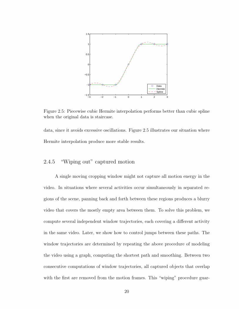
2.5 Piecewise cubic Hermite interpolation performs better than cubicspline when the original data is staircase. . . . . . . . . . . . . . . . . 20
2.6 Example of merging three windows trajectories. The horizontal axisrepresents time; the thick lines are for the segments of the trajectoriespicked at that time; and the dashed lines are for times where jumpsoccur. . . . . . . . . . . . . . . . . . . . . . . . . . . . . . . . . . . . 21
2.7 Four typical frames from an airport surveillance video, with threetrajectories and fixed window size. In each frame, the original videoframe, showing the locations of the cropping windows, is to the leftand the cropped frame is to the right, resized to the original’s height. 24
2.8 Two typical frames from a traffic intersection surveillance video, withtwo trajectories and fixed window size. In each frame, the originalvideo frame, showing the locations of the cropping windows, is to theleft and the cropped frame is to the right, resized to the original’sheight. . . . . . . . . . . . . . . . . . . . . . . . . . . . . . . . . . . . 25
2.9 Variable size single trajectory results. Compared to the fixed sizeresults, less empty area is retained around small cropped objects. . . 25
2.10 Video-in-video results: the cropped video location is selected auto-matically in the boundary region of overall least activity. . . . . . . . 25
2.11 Multi-camera display issues should be addressed in later work. Orig-inal video to the left; cropped video to the right. . . . . . . . . . . . . 26
v

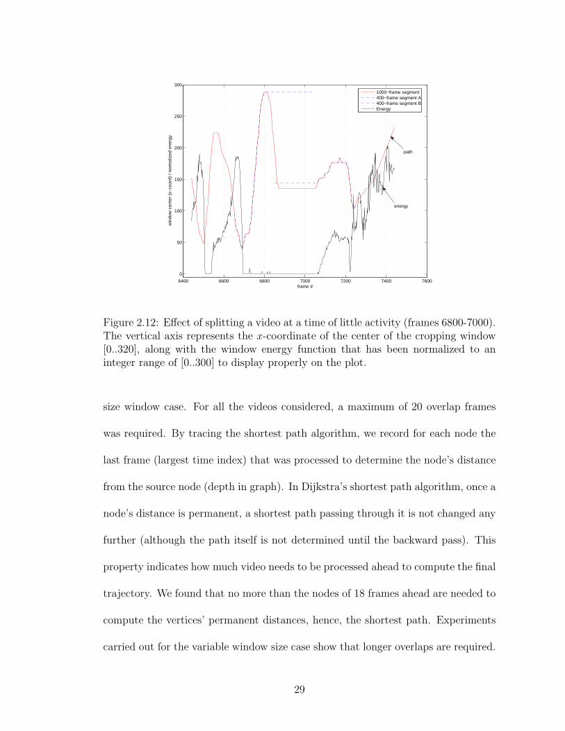
2.12 Effect of splitting a video at a time of little activity (frames 6800-7000). The vertical axis represents the x-coordinate of the center ofthe cropping window [0..320], along with the window energy functionthat has been normalized to an integer range of [0..300] to displayproperly on the plot. . . . . . . . . . . . . . . . . . . . . . . . . . . . 29
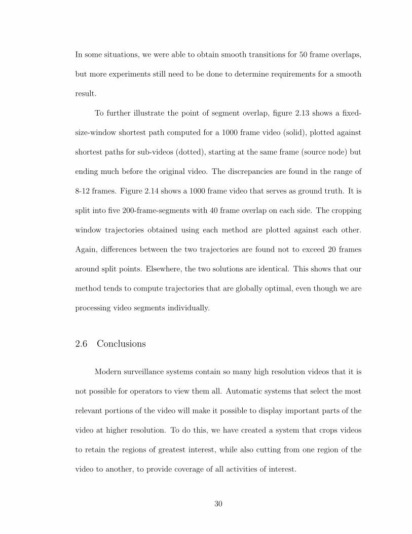
2.13 Shortest paths of video prefixes. . . . . . . . . . . . . . . . . . . . . . 31
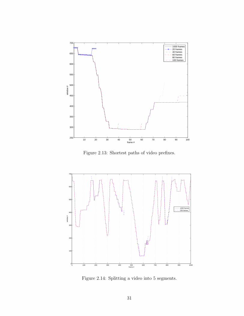
2.14 Splitting a video into 5 segments. . . . . . . . . . . . . . . . . . . . . 31
2.15 A cropped frame resulting from panning across a largely empty scene(left: original frame, showing the location of the cropping window;right: cropped frame). . . . . . . . . . . . . . . . . . . . . . . . . . . 33
3.1 Problem setup in 2D. People’s trajectories are dotted and visibilitypolygons are in blended colors. The obstacles are shaded in black. . . 40
3.2 Computing the visibility polygon: rays r2 and r4 are tangent to ob-stacles, while r3 and r5 intersect them. . . . . . . . . . . . . . . . . . 42
3.3 Computing occlusions of subjects by one another. . . . . . . . . . . . 43
3.4 An example of the problem model with a perfect matching. . . . . . . 45
3.5 A bipartite graph update that involves the two cases with edge re-moval. Matched edges are thickened. In the first update, a non-matched edge v1u1 is removed so nothing needs to be done. In thesecond time, the matched edge v2u2 is removed. The alternating pathv2u4v3u2 (red) matches v2u4, unmatches v3u4 and matches v3u2. . . . 47
3.6 A bipartite graph update that involves the addition of an edge toan incomplete matching. Matched edges are thickened. Initially, themaximum possible matching is incomplete. Later, an edge v4u1 isadded. This permits completing the matching using the alternatingpath v4u1v3u2 . . . . . . . . . . . . . . . . . . . . . . . . . . . . . . . 47
3.7 The approach used to cluster people. The cardinalities of the inter-sections are marked to the left and the actual clusters to the right. . . 49
3.8 Two example setups used in testing our method. Left: inside a bank,generated using our simulator (overlapping field-of-regard cameras);Right: a grid of obstacles, generated using van den Berg’s simulator.The linear segments are people’s trajectories. . . . . . . . . . . . . . . 54
vi

3.9 Mean coverage as the group size (diameter) varies. Top: bank sce-nario from our simulator. Bottom: regular grid of obstacles from vanden Berg’s simulator. . . . . . . . . . . . . . . . . . . . . . . . . . . . 56
3.10 Effect of adding a time penalty on the standard deviation (=√
var)of the coverage. Top: bank scenario (our simulator) with a group sizeequal to 5 people. Bottom: regular grid of obstacles (van den Berg’ssimulator) without grouping. . . . . . . . . . . . . . . . . . . . . . . . 57
3.11 Matching times for various graph sizes (van den Berg’s simulator). . . 58
3.12 Snapshot of our simulator: 2D top view with visibility regions alongwith 3D zoomed-in videos for the first 3 subjects. . . . . . . . . . . . 58
4.1 A simplified layout that shows polygonal obstacles, players (points)and the environment partition with a grid. . . . . . . . . . . . . . . . 65
4.2 A Euclidean-distance neighborhood of radius 2 centered around theblack square. . . . . . . . . . . . . . . . . . . . . . . . . . . . . . . . 66
4.3 A Manhattan-distance neighborhood of radius 2 centered around theblack square. . . . . . . . . . . . . . . . . . . . . . . . . . . . . . . . 66
4.4 Initial winning positions for a level-0 game. . . . . . . . . . . . . . . . 68
4.5 Initial losing positions for a level-0 game. . . . . . . . . . . . . . . . . 68
4.6 Computing the labeling function Bad(N(p), e, 0) for the neighbor-hood of a pursuer located at position p, where p′ and p′′ are the onlypossible neighbors for p due to the obstacle. . . . . . . . . . . . . . . 69
4.7 Extending Bad(N(p), e, 0) into Bad(p, e, 1). Steady state is reachedat that point. . . . . . . . . . . . . . . . . . . . . . . . . . . . . . . . 70
4.8 An example of a level-1 game where the pursuer loses in 2 steps. . . . 71
4.9 Computing the labeling function Bad(N(p), e, 0) for the neighbor-hood of a pursuer located at position p, where p′ and p′′ are the onlypossible neighbors for p due to the obstacle. . . . . . . . . . . . . . . 71
4.10 Extending Bad(N(p), e, 0) into Bad(p, e, 1). . . . . . . . . . . . . . . 72
4.11 Computing the labeling function Bad(N(p), e, 1) out of the mapsBad(pi, e, 1) for neighbors of position p. . . . . . . . . . . . . . . . . . 72
4.12 Extending Bad(N(p), e, 1) into Bad(p, e, 2). Steady state is reachedat that point. . . . . . . . . . . . . . . . . . . . . . . . . . . . . . . . 73
vii

5.1 Introductory example that shows the type of anomalies we are inter-ested in. The first two events are usual, but the third is not. Althoughit consists of a combination of exactly the two left event, it is theirsimultaneous occurrence that make it unusual . . . . . . . . . . . . . 79
5.2 The small (yellow) filled circles represent humans. A single person us-ing the trash bin (a) or two people meeting in the building’s lobby (b)are considered usual situations. On the other hand, people meetingnext to the trash bin (c) is an unusual situation. . . . . . . . . . . . . 86
5.3 Typical snapshot of our 4-way stop sign simulator. Arrows indicatethe driving directions and squares represent vehicles. Cars are notstrictly aligned due to the simulated noise. . . . . . . . . . . . . . . . 91
5.4 Typical distribution functions for a 16-bin grid. The pair of bins withthe shown distribution in (a) observe relatively high joint activity,while (b) is for a pair of bins between which only one type of activityis present. Both plots are for the probability versus the event valueindex. . . . . . . . . . . . . . . . . . . . . . . . . . . . . . . . . . . . 93
5.5 Example of detected unusual events. The bin(s) where the eventoccurred is highlighted. In (a), the left and the right vehicles areeach attempting to make a left turn simultaneously and are aboutto collide. In (b), the upper vehicle is making a left coinciding withthe lower vehicle making a right. This will result in the two vehiclesdriving very close to one another. . . . . . . . . . . . . . . . . . . . . 94
5.6 First order anomaly example: a U-turn. Regardless of its interactionwith other cars, a U-turn is not allowed (unusual) at a stop sign.Without noting this fact (a), it is reported as unusual w.r.t. mostother populated bins. The algorithm has been updated to filter outfirst order events from further processing with other bins (b). . . . . . 95
5.7 Unusual event detection using a coarse grid with 16 bins (a) and afine one in (b). The mean correct detection rate is plotted versusthe mean false alarm rate. For the coarse grid (a), the introductionof noise slightly deteriorates the detection rate, but for appropriatechoices of pth the method proves to be immune to noise. The fine grid(b) is very sensitive to noise. In this case, adapting between coarseand fine grids can be the best alternative. . . . . . . . . . . . . . . . 96
5.8 Unusual event detection: coarse and fine grids compared in the ab-sence of noise. Slightly better performance using the fine grid formany values of pth. . . . . . . . . . . . . . . . . . . . . . . . . . . . . 97
5.9 Typical video snapshot showing the 3 types of detected objects . . . . 98
viii

5.10 Three examples of tracking errors: (a) three adjacent pedestrians clas-sified as a vehicle. (b) Missed pedestrian. (c) Moving tree branchesand empty parking spot detected as moving objects. . . . . . . . . . . 99
A.1 Overlapping-rates on the Nova Animal Set (4509 images) using dif-ferent algorithms. . . . . . . . . . . . . . . . . . . . . . . . . . . . . . 107
A.2 Overlapping-rates on the Nova Animal Set of two manual croppings. . 108
A.3 Scatter plot of rectangle area versus saliency content. . . . . . . . . . 108
A.4 Statistics of hand cropping for the “non-professional” set. . . . . . . . 109
ix

Chapter 1
Introduction
1.1 Motivation
The use of video surveillance systems has been rising over the past decade.
Most recently, the need to improve public safety and the concerns about terrorist
activity have contributed to a dramatic increase in the demand for surveillance sys-
tems. The presence of these systems is very common in airports, subways, metropoli-
tan areas, seaports, and in areas with large crowds. Modern video surveillance sys-
tems consist of networks of cameras connected to a control room that includes a
collection of monitors. Typical control rooms have a much smaller number of moni-
tors than cameras and far fewer operators than monitors. The monitors either cycle
automatically through the cameras, or operators can manually choose any camera
from the network and display it on a selected monitor.
The M25 London Orbital highway system consists of 5 traffic control centers,
each with 60 monitors connected to 324 cameras and distributed over 70 sites. The
London underground has a network of 25,000 cameras at 167 stations [1]. A recent
survey by the New York Civil Liberties Union found that in Lower Manhattan,
New York City, the number of surveillance cameras below 14th St grew from 769
in 1998 to 4176 in 2005. According to the same source, the New York City Police
Department announced in 2006 that it planned to create a “citywide system of
1

Figure 1.1: Typical design of a control room
closed circuit televisions” operated from a single control center [2]. In the area of
crowd control, CNN News reported from inside the central surveillance control room
for this year’s Hajj ritual at Mecca, Saudi Arabia. Over 1400 cameras monitored
a crowd of around 3 million pilgrims, who can flow in some areas at rates of up to
250,000 per hour [3]. A typical design of a control room is illustrated in figure 1.1.
We suggest this work to be part of a larger project in the design of future
control rooms, that envisions an architecture consisting of a large display wall which
acts as a single entity, as opposed to matrices of independent monitors, or display
regions with pre-specified monitoring tasks, as in current state of the art control
rooms. The display wall assigns variable areas and locations to a subset of the
available videos from surveillance cameras. The problem of selecting the subset
of videos to display is addressed in this dissertation. Here, we do not only mean
2

the automatic selection of a camera footage to display at a specific time. We go
one step further by editing the individual videos in both time and space before
displaying them, possibly stitching together different video “pieces” coming from
different cameras. Our goal is to present the operators with a video that contains
the most critical scenes of the surveyed environment, thus focusing their attention on
important information content. The related problems of assigning the appropriate
area and selecting the location where the edited video is to be displayed is motivated
in this dissertation, but the details are rather left as an area of future research.
Intuitively, video segments that are more interesting to human operators shall be
assigned longer display times, larger areas and more prominent parts of the display
wall. Some “scoring” mechanism will be used to achieve this task. An overview of
the surveillance system’s architecture presented in this dissertation is illustrated in
figure 1.2.
1.2 Dissertation Organization
In this dissertation, we present four components that collaborate in building
our proposed surveillance system. First, we note that assigning a video to its display
area typically requires resizing it. If the assigned space is small, simply reducing
the resolution of the original video might render its contents to be illegible. In
this situation, cropping the video before resizing it results in videos that should be
easier for humans to interpret. This brings up the need to automatically edit the raw
footage coming from cameras. The design and implementation of this component,
3
Scoring
Mapping
Display Wall
Cropping
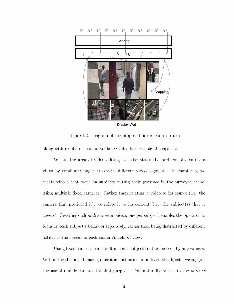
Figure 1.2: Diagram of the proposed future control room
along with results on real surveillance video is the topic of chapter 2.
Within the area of video editing, we also study the problem of creating a
video by combining together several different video segments. In chapter 3, we
create videos that focus on subjects during their presence in the surveyed scene,
using multiple fixed cameras. Rather than relating a video to its source (i.e. the
camera that produced it), we relate it to its content (i.e. the subject(s) that it
covers). Creating such multi-camera videos, one per subject, enables the operator to
focus on each subject’s behavior separately, rather than being distracted by different
activities that occur in each camera’s field of view.
Using fixed cameras can result in some subjects not being seen by any camera.
Within the theme of focusing operators’ attention on individual subjects, we suggest
the use of mobile cameras for that purpose. This naturally relates to the pursuer
4

evader game. The first question that comes to mind is whether or not a pursuer
will be able to maintain the visibility of an evader at all times and for which initial
positions of the players. We devise an algorithm to solve that problem in chapter
4 and, if the answer to the question of maintaining the visibility of the evader is
affirmative, we also compute the motion strategy that realizes this.
Finally, chapter 5 presents our method to detect anomalous activity in video.
By identifying time intervals and locations of unusual activity, we present yet another
method of focusing the operator’s attention on interesting parts of surveillance video
that could require further human intervention.
1.3 Contributions
We have introduced several novel methods in analyzing surveillance video in
this dissertation. In the area of video editing, we defined and implemented a broader
video cropping technique that deals with raw camera footage versus retargeting pre-
edited video. We also introduced a new approach to solve the problem of tracking
people across multiple cameras. We applied our method to a new problem of auto-
matically creating a video for a subject from the footage of multiple cameras.
In the area of pursuer-evader games, we have developed a new computationally
feasible approach to solve the problem of determining the outcome of the game. Fi-
nally, our anomaly detection method uses co-occurrence statistics of moving objects
in time and space. Unlike earlier approaches that used co-occurrence statistics in
time only, our method is able to detect additionally events that need not be unusual
5

if considered individually, but that become so when occurring simultaneously.
6

Chapter 2
Automatic Video Editing
2.1 Introduction
In surveillance applications, video cropping helps to focus the attention of
operators on specific parts of the scene. Activity occurring in the background or at
corners of the display area might pass unnoticed by operators, due to other activity
in more prominent areas of the scene. Cropping is often needed as well to save
bandwidth in transferring the video or saving it for archiving purposes. The tradeoff
here is between the size of the cropped video and the information loss. In scenes
with several regions of simultaneous activity, allowing the cropping window to jump
occasionally between these regions supports coverage of multiple activities, while
keeping the resulting cropped video small. In addition, it is crucial in surveillance
applications to process video online −as it becomes available− and cannot require
the entire video to be available beforehand. These points are amplified in the body
of this chapter.
We define the video cropping problem to be the determination of a smooth
path of a cropping window that captures “salient” foreground throughout the video.
The window can have variable size, which introduces virtual zoom-in and zoom-out
effects. It is allowed occasional jumps through the video, similar to scene cuts in
filmmaking. We use motion energy as a measure of the “saliency” of a cropping
7
window trajectory. Unlike previous approaches, we optimize the saliency globally
for the whole trajectory, rather than for individual frames or shots, as follows.
First, the video is modeled as a graph of windows, with its edge weights
reflecting saliency captured by windows, efficiently computed using integral images
[78]. Then, a shortest path algorithm finds the window trajectory that captures the
overall maximum motion energy. The resulting trajectory is smoothed to remove
jiggles and staircase-like appearance. This procedure is repeated several times on
the remaining parts of the video to capture the remaining saliency. This results in
obtaining a set of disjoint smooth paths of cropping windows that capture as much
saliency as possible. A secondary optimization procedure produces the final path
by alternately jumping between the paths computed earlier, selecting which one to
follow at which time, so as to maximize both captured saliency and covered regions of
the original video. Long videos are processed by breaking them into manageable sub-
videos, while allowing overlap between consecutive subvideos, to produce smooth
transitions. Our algorithm is applied to a collection of real surveillance videos.
Several experiments are performed to determine the optimal choices regarding issues
such as where to cut a video into sub-videos, the amount of overlap between them
and how long a segment should be displayed before jumping to another. Some
display configurations are compared, such as cropped video alone, side by side with
original video, or video-in-video (like commercially available picture-in-picture).
We are mainly interested in surveillance applications. Typically, much more
video than operators can observe is available. In addition, this video is unedited,
and more importantly, not focused on any agent in the scene. This has made our
8

approach [21] different from earlier approaches that dealt with edited videos, such
as movies, news reports, or classroom video. In particular, our method offers the
following contributions:
• a variable size cropping window which results in a smooth zoom in/out effect,
• multiple cropping windows to cover more agents in the scene,
• only a relatively short video segment needs to be processed at a time −not
the complete video− which makes the algorithm an online algorithm, and
• we show empirically that by stitching together results from short segments of
a video, we get a result identical to the globally optimal one, given the entire
video.
The rest of this chapter is organized as follows: section 2.2 reviews related
work. Then, the video cropping problem is formally defined in section 2.3. In
section 2.4, we present our approach to solve the problem, while section 2.5 presents
the results. Finally, closing remarks and conclusions can be found in section 2.6.
2.2 Related Work
Research has been performed in the area of visual attention to detect salient
areas in images and video from low-level features. Itti et al. [41] use orientation
filters in addition to color and intensity to detect salient parts of images. Later,
Itti and Baldi extend this method to work with videos, using a statistical model
for time [40]. A probabilistic approach is used by Kadir and Brady as a measure
9
of local saliency in images [42]. Their method is generalized by Hung and Gong by
including the time variable to quantify spatio-temporal saliency in videos [38].
Many methods for cropping still images automatically have been published.
For example, Suh et al. [68] use Itti’s saliency model, along with face detection, to
crop informative parts of images before reducing them to thumbnails. The same
model is also used by Chen et al. [12], with the addition of text detection, to find
regions of interest in images for adaptation to small displays. Xie et al. [83] study
the statistics of users’ interaction with images on small displays to determine regions
of maximum user interest.
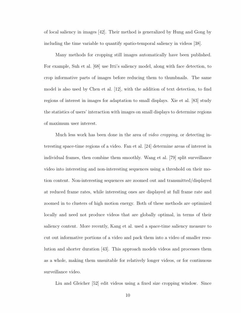
Much less work has been done in the area of video cropping, or detecting in-
teresting space-time regions of a video. Fan et al. [24] determine areas of interest in
individual frames, then combine them smoothly. Wang et al. [79] split surveillance
video into interesting and non-interesting sequences using a threshold on their mo-
tion content. Non-interesting sequences are zoomed out and transmitted/displayed
at reduced frame rates, while interesting ones are displayed at full frame rate and
zoomed in to clusters of high motion energy. Both of these methods are optimized
locally and need not produce videos that are globally optimal, in terms of their
saliency content. More recently, Kang et al. used a space-time saliency measure to
cut out informative portions of a video and pack them into a video of smaller reso-
lution and shorter duration [43]. This approach models videos and processes them
as a whole, making them unsuitable for relatively longer videos, or for continuous
surveillance video.
Liu and Gleicher [52] edit videos using a fixed size cropping window. Since
10

they focus mainly on editing feature films, the window moves are restricted to pans
and cuts whose parameters are optimized over individual shots. To keep the original
structure of the film, the authors introduce a set of heuristic penalties that limit
the motion of the cropping window. Although this approach works well with pro-
fessionally captured films, it may not generalize well to unedited raw surveillance
video, which generally have wider fields of view, are not focused on a main subject,
and consist of a single shot. Within the same area of cropping television and cinema
video content to fit a different screen size, Deselaers et al. [15] also scan the video
using a fixed size cropping window. They occasionally zoom-out, padding with black
borders, when the cropping window “is not able to capture all relevant parts of the
image”. Another recent example of automatic editing of specific types of videos is
that of classroom video editing. Heck et al. [32] find an optimal shot sequence, from
a set a virtual shots, that have been selected based on prior knowledge of the scene
and video content.
2.3 Problem definition
Given a video sequence, our goal is to determine a smooth trajectory for a
variable size window through the video, that maximizes the captured saliency over
all such trajectories and window sizes. Occasional jumps are allowed to include as
much saliency as possible. More formally, we consider the problem of optimizing a
single trajectory. Assume the input video segment has T frames. Each frame t can be
covered by a set of n variable size overlapping windows. These windows are labeled
11
Wi,t, with i being the window number, selected from an index set I = {1, 2, . . . , n}.
Define the cross product set I = I × I × · · · × I = IT . Then, we want to solve the
problem:
arg maxQ
∑t
S(Wi,t) (2.1)
where S(·) is a saliency measure, Q ∈ I is the window sequence that maximizes the
saliency, and i ∈ I. It is more desirable to minimize functions, thus, the saliency
function S(·) can be replaced by a cost function C(·) that decays with increasing
saliency. Model (2.1) doesn’t enforce spatial smoothness. To guarantee a smooth
path, windows in two consecutive frames are restricted to be close to one another
and with little area variation. The problem is thus formulated as:
arg minQ
∑t
C(Wi,t) (2.2)
such that: d(Wi′,t−1,Wi,t) < dmax
|A(Wi′,t−1)−A(Wi,t)| < Amax
where d(·, ·) is a distance measure and A(W ) is the area of window W .
Our main contribution [21] is that we optimize globally, over the whole video,
rather than locally for individual frames, that are later combined. This approach
maximizes the total captured saliency and provides smoother results.
2.4 Video Cropping Approach
Solving problem (2.2) by trying all possible paths is prohibitively expensive.
Instead, we employ a dynamic programming approach, using the following proce-
dure. First, motion energy is extracted through frame differences. Then, we build a
12

Extract Motion Energy
BuildingGraph
WipingFrames
MergingTrajectories
ShortestPath +
Smoothing
Video
Frames
FramesMotion
Trajectories Cropped
Video
Figure 2.1: Overview of our approach to crop a video segment.
weighted directed graph, with the cropping windows as its vertices, and edge weights
measuring the motion energy. A shortest path algorithm through the graph selects
the first optimal trajectory, which minimizes equation (2.2). This trajectory is then
smoothed, and the motion it contains is “wiped out” from the original frames. This
procedure is repeated to capture some of the remaining energy. A second graph is
built out of the resulting trajectories with shortest path run once again to deter-
mine the optimal combination of paths. In the final cropped video, one trajectory
is followed at a time, with occasional jumps between these trajectories. For long
videos, video segments are chosen to overlap with their immediately preceding ones,
and are processed similarly. This allows smooth transitions between the respective
trajectories in each segment. The whole process is summarized in figure 2.1. In the
remainder of this section, the above steps are presented in more detail.
2.4.1 Extracting motion energy
In our implementation, we use motion energy as a measure of saliency. Earlier
approaches [24, 52] used centered frame saliency maps, face and text detectors in
addition to motion contrast, to crop movies and news. These detectors are too
specific to be used with surveillance video.
13

Motion energy is efficiently computed in real time, and captures important
activity in surveillance video. We compute frame differences and threshold them to
detect motion, then apply morphological operations to the resulting motion frames.
In particular, the opening operation is applied to remove detected small noisy areas,
then a closing operation connects nearby fragments. The motion energy is computed
to be the number of 1’s in the resulting binary images. The remainder of the
algorithm works on these preprocessed difference frames.
2.4.2 Building the graph
The video is modeled as a weighted directed graph as follows. Let G = (V,E)
be the graph. Each frame is sampled by n overlapping cropping windows of various
sizes. Then, each window is represented by a vertex v ∈ V. This makes the total
number of vertices in the graph |V| = nT for a video segment of T sample frames.
The restrictions in the problem formulation (2.2) are implemented by allowing a
window to move only to neighboring window positions, or to grow or shrink by no
more than one size step between two consecutive frames. This translates to adding
an edge to E only if it connects a pair of vertices that represents a pair of windows
between which a step is allowed. For a certain ordering of the vertices V, the
adjacency matrix of G is banded. This is a sparse matrix that can be efficiently
stored using an adjacency list graph representation, to store just the bands. With
b ¿ nT neighbors allowed per window, we have a graph of O(nT ) edges. An
additional “source” node and a “target” node are added to the beginning and end
14
dummysourcenode
dummytargetnode
w=0 w=0
w=0w=0
nodesof firstframe
nodesof lastframe
nodesof frame i
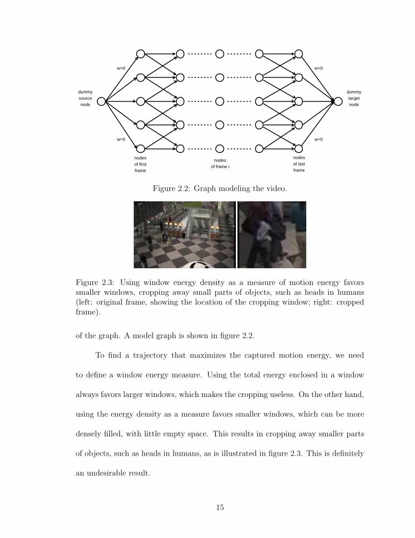
Figure 2.2: Graph modeling the video.
Figure 2.3: Using window energy density as a measure of motion energy favorssmaller windows, cropping away small parts of objects, such as heads in humans(left: original frame, showing the location of the cropping window; right: croppedframe).
of the graph. A model graph is shown in figure 2.2.
To find a trajectory that maximizes the captured motion energy, we need
to define a window energy measure. Using the total energy enclosed in a window
always favors larger windows, which makes the cropping useless. On the other hand,
using the energy density as a measure favors smaller windows, which can be more
densely filled, with little empty space. This results in cropping away smaller parts
of objects, such as heads in humans, as is illustrated in figure 2.3. This is definitely
an undesirable result.
15
E in
E belt
1
4 3
2
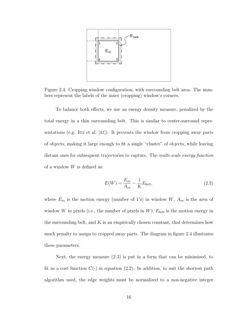
Figure 2.4: Cropping window configuration, with surrounding belt area. The num-bers represent the labels of the inner (cropping) window’s corners.
To balance both effects, we use an energy density measure, penalized by the
total energy in a thin surrounding belt. This is similar to center-surround repre-
sentations (e.g. Itti et al. [41]). It prevents the window from cropping away parts
of objects, making it large enough to fit a single “cluster” of objects, while leaving
distant ones for subsequent trajectories to capture. The multi-scale energy function
of a window W is defined as:
E(W ) =Ein
Ain
− 1
KEbelt, (2.3)
where Ein is the motion energy (number of 1’s) in window W , Ain is the area of
window W in pixels (i.e., the number of pixels in W ), Ebelt is the motion energy in
the surrounding belt, and K is an empirically chosen constant, that determines how
much penalty to assign to cropped away parts. The diagram in figure 2.4 illustrates
these parameters.
Next, the energy measure (2.3) is put in a form that can be minimized, to
fit as a cost function C(·) in equation (2.2). In addition, to suit the shortest path
algorithm used, the edge weights must be normalized to a non-negative integer
16
range. We choose this range to be from 0 to 100. If a transition is allowed from
vertex i to vertex j, an edge is added to the graph with weight w(i, j) computed as:
w(i, j) =
⌊100− 100 max
(Ej
Aj
− 1
KEbeltj , 0
)+ 0.5
⌋(2.4)
where Ej, Aj and Ebeltj are all related to the window represented by vertex j. The
function bx + 0.5c rounds x to the nearest integer. Ej and Ebeltj are computed by
summing the motion pixels (1’s) for each window in each pre-processed difference
frame. This is a time consuming operation if performed in a straightforward manner.
Instead, we use integral images in a manner similar to Viola and Jones in image
analysis [78] based on an idea by Crow for texture mapping [14]. Given an image
i(x, y), the integral image ii accumulates pixels to the top and left of each pixel, as
defined by:
ii(x, y) =∑
x′≤x,y′≤y
i(x′, y′).
The integral image is computed in one pass using the two recurrences:
s(x, y) = s(x, y − 1) + i(x, y) (row sum)
ii(x, y) = ii(x− 1, y) + s(x, y) (integral image)
s(x,−1) = 0 ; ii(−1, y) = 0
The integral image is computed once for every frame, then every window sum, Ej, is
computed using only 4 operations. Thus, we avoid computing the cumulative sum
for each window, which includes a lot of redundancy due to the overlap between
windows. Given a window with corners −→x1, −→x2, −→x3 and −→x4 in clockwise direction,
starting from the top left (see figure 2.4), the cumulative sum in that window can
17
be computed as:
ii(−→x3)− ii(−→x2)− ii(−→x4) + ii(−→x1).
2.4.3 Shortest path
The shortest path from the source node to the target node is computed using
Dijkstra’s algorithm [17]. Benefiting from the special structure of this graph, some
modifications are introduced into the algorithm to improve performance. Early
termination can be achieved by halting the search prematurely when the first vertex
(window) in the last video frame is reached, rather than waiting until all the vertices
in the graph are labeled.
Dijkstra’s algorithm is mainly slowed down by the search for the closest vertex
to the source, in a list of temporary labeled nodes, at each iteration. With N vertices
in the graph, the asymptotic running time of the algorithm is O(N2) orO(N log(N))
depending on the data structure used to implement the list of temporary labeled
nodes. This running time has been reduced in our implementation in two ways. The
multiplying factor is directly affected by the size of the list of temporary labeled
nodes. In our runs, we note that the maximum number of nodes in that list, over
all iterations, is just around 1% of the total number of vertices in the graph.
The running time is also reduced an order of magnitude, from quadratic to
linear in the number of vertices, using Dial’s implementation [16]. In the original
algorithm, Dial stores temporarily labeled nodes in buckets, indexed by the nodes’
distances. This makes the search for the minimum distance node O(1). With
18
C being the maximum edge weight (100 in our graph), Dial’s original algorithm
maintains NC + 1 buckets, which may be prohibitively large. A remark made
by Ahuja [7] reduces the space requirements to only C + 1 buckets. During each
iteration, the difference between the maximum and minimum finitely labeled nodes
cannot exceed C. Hence, temporarily labeled nodes can be hashed by their distance
labels into just C + 1 buckets.
2.4.4 Smoothing
The shortest path resulting from the previous stage has a noisy appearance,
which can be best compared to a jittery or shaking cameraman, from the point of
view of the cropped video. Two levels of smoothing are applied to the trajectory.
First, a moving average smoother is applied to the trajectory. With y(t) being the
original data (raw trajectory) at time t and ys(t) the smoothed one, the difference
equation is:
ys(i) =1
2N + 1(y(i + N) + y(i + N − 1) + · · ·+ y(i−N)) ,
where N is the “radius” of the span interval. This has the effect of a lowpass filter,
reducing the shaky appearance of the trajectory. Truncating the result completely
removes any such artifacts, but results in a staircase-like appearance. A second
level of smoothing is done by interpolating a piecewise cubic Hermite polynomial
to a sub-sampled version of the data. This polynomial interpolates the data points
and has a continuous first derivative. However, unlike cubic splines, the second
derivative need not be continuous. This property is more suitable for our staircase
19
−3 −2 −1 0 1 2 3−1.5
−1
−0.5
0
0.5
1
1.5
DataHermiteSpline
Figure 2.5: Piecewise cubic Hermite interpolation performs better than cubic splinewhen the original data is staircase.
data, since it avoids excessive oscillations. Figure 2.5 illustrates our situation where
Hermite interpolation produce more stable results.
2.4.5 “Wiping out” captured motion
A single moving cropping window might not capture all motion energy in the
video. In situations where several activities occur simultaneously in separated re-
gions of the scene, panning back and forth between these regions produces a blurry
video that covers the mostly empty area between them. To solve this problem, we
compute several independent window trajectories, each covering a different activity
in the same video. Later, we show how to control jumps between these paths. The
window trajectories are determined by repeating the above procedure of modeling
the video using a graph, computing the shortest path and smoothing. Between two
consecutive computations of window trajectories, all captured objects that overlap
with the first are removed from the motion frames. This “wiping” procedure guar-
20
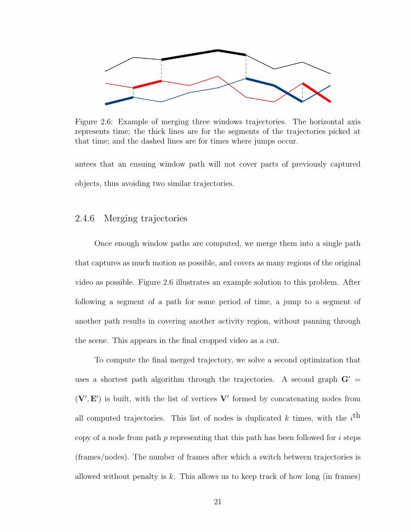
Figure 2.6: Example of merging three windows trajectories. The horizontal axisrepresents time; the thick lines are for the segments of the trajectories picked atthat time; and the dashed lines are for times where jumps occur.
antees that an ensuing window path will not cover parts of previously captured
objects, thus avoiding two similar trajectories.
2.4.6 Merging trajectories
Once enough window paths are computed, we merge them into a single path
that captures as much motion as possible, and covers as many regions of the original
video as possible. Figure 2.6 illustrates an example solution to this problem. After
following a segment of a path for some period of time, a jump to a segment of
another path results in covering another activity region, without panning through
the scene. This appears in the final cropped video as a cut.
To compute the final merged trajectory, we solve a second optimization that
uses a shortest path algorithm through the trajectories. A second graph G′ =
(V′,E′) is built, with the list of vertices V′ formed by concatenating nodes from
all computed trajectories. This list of nodes is duplicated k times, with the ith
copy of a node from path p representing that this path has been followed for i steps
(frames/nodes). The number of frames after which a switch between trajectories is
allowed without penalty is k. This allows us to keep track of how long (in frames)
21
a single trajectory has been followed.
There always exists an edge e ∈ E′ from every node to the next node in the
same path, and edges to next frame nodes in the other paths if a “cut” is allowed
at that time. The weight function w′ is the cost associated with the representative
window in the original graph G, computed as in (2.4), if the edge connects two
nodes in the same path. However, if a path switch occurs, a penalty function
is added to that weight. Intuitively, a higher penalty is associated with switches
to closer trajectories, to favor more coverage of the original video, and to avoid
“jumps”. Another penalty is added to the window cost, that decays with the time
that has been spent following a certain trajectory. This latter penalty inhibits
frequent successive cuts, which might distract the operator. These penalties are
fractions of the window cost, to make them comparable to the window cost penalty
(2.2) in the global optimization. They are determined empirically, based on runs
conducted on several videos. We also noticed that these penalties are consistent with
filmmakers’ heuristics, who might use frequent cuts purposely only when special
“pacing effects” are required. Similarly, filmmakers would avoid a cut to a nearby
location, which is known in cinematography as a “jump cut”. These rules have been
followed in feature film editing [52] when creating virtual cuts.
2.4.7 Processing long videos
Real-time surveillance applications require online processing of video. Ad-
ditionally, available processing resources constrain the longest video that can be
22
processed as a whole. Our approach allows us to process long videos by breaking
them into segments, with some overlap. Each segment is processed separately, re-
sulting in consecutive overlapping trajectories. By piecing together corresponding
paths from each segment and removing the overlap, continuous smooth trajectories
result. This is further discussed in the section on results, where experiments are
performed to determine appropriate locations to break the video into segments and
the amount of overlap needed for smooth transitions.
2.4.8 Video display
Several display methods for the resulting cropped video are considered. The
most obvious is just displaying the cropped region. This is the most space efficient
but may result in seeing the cropped video out of its context. To keep both context
and content, we display both the original and cropped videos side by side, with
the original one shrunk to fit the display space. This display method is not space
efficient, though.
To display context, while keeping a reasonable video size, we suggest a video-
in-video display style. The familiar style is to display the “sub”-video (cropped
video here) in a corner of the “full” video. In our approach, we find the optimal
display location automatically while computing the shortest path. It is chosen to
be largest border window, that covers the minimum activity in the video. In terms
of our implementation, this is the largest window on the border that contains the
least motion energy. The video-in-video window is of fixed size and location, but
23
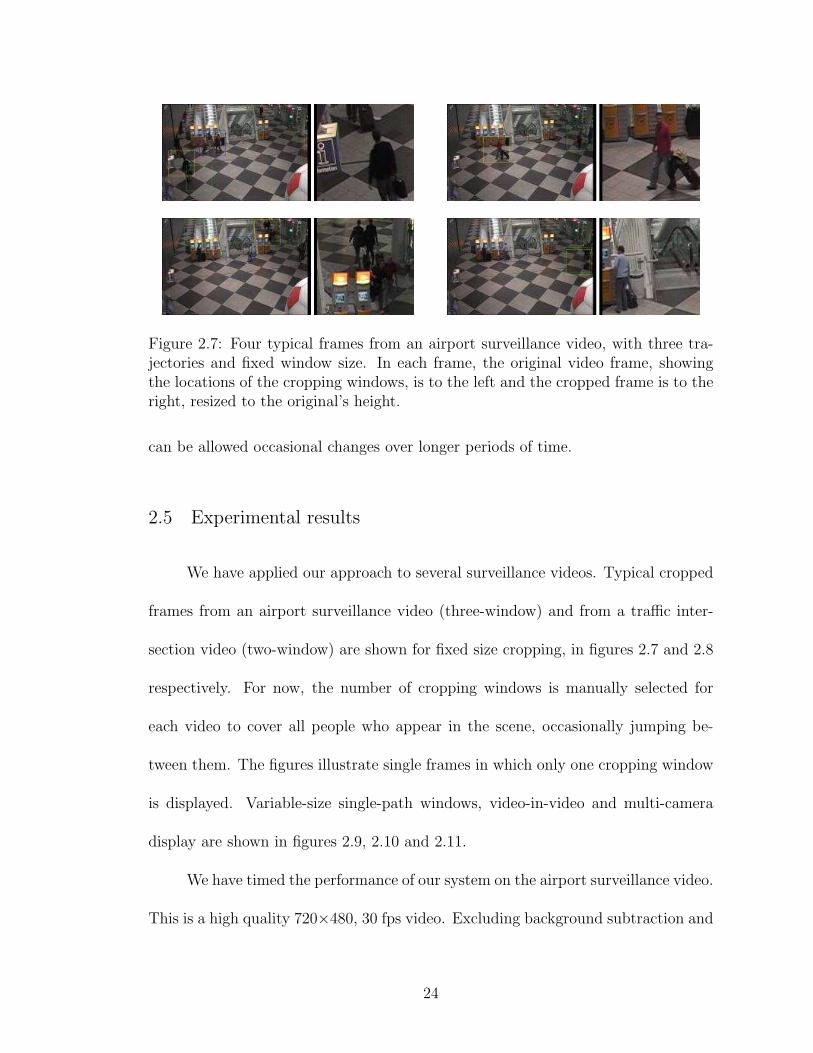
Figure 2.7: Four typical frames from an airport surveillance video, with three tra-jectories and fixed window size. In each frame, the original video frame, showingthe locations of the cropping windows, is to the left and the cropped frame is to theright, resized to the original’s height.
can be allowed occasional changes over longer periods of time.
2.5 Experimental results
We have applied our approach to several surveillance videos. Typical cropped
frames from an airport surveillance video (three-window) and from a traffic inter-
section video (two-window) are shown for fixed size cropping, in figures 2.7 and 2.8
respectively. For now, the number of cropping windows is manually selected for
each video to cover all people who appear in the scene, occasionally jumping be-
tween them. The figures illustrate single frames in which only one cropping window
is displayed. Variable-size single-path windows, video-in-video and multi-camera
display are shown in figures 2.9, 2.10 and 2.11.
We have timed the performance of our system on the airport surveillance video.
This is a high quality 720×480, 30 fps video. Excluding background subtraction and
24
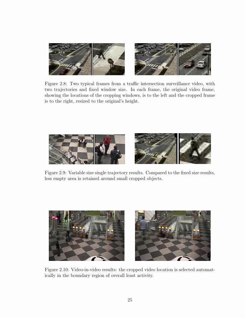
Figure 2.8: Two typical frames from a traffic intersection surveillance video, withtwo trajectories and fixed window size. In each frame, the original video frame,showing the locations of the cropping windows, is to the left and the cropped frameis to the right, resized to the original’s height.
Figure 2.9: Variable size single trajectory results. Compared to the fixed size results,less empty area is retained around small cropped objects.
Figure 2.10: Video-in-video results: the cropped video location is selected automat-ically in the boundary region of overall least activity.
25
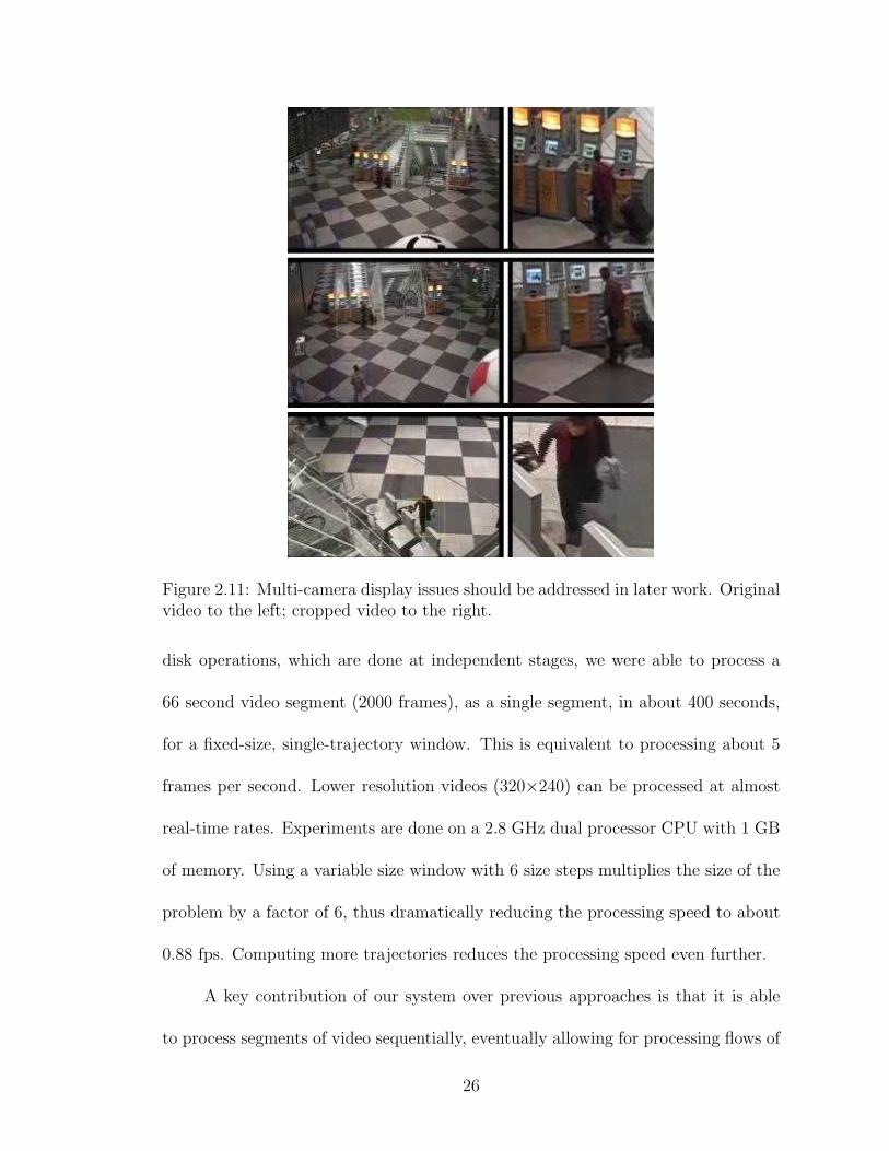
Figure 2.11: Multi-camera display issues should be addressed in later work. Originalvideo to the left; cropped video to the right.
disk operations, which are done at independent stages, we were able to process a
66 second video segment (2000 frames), as a single segment, in about 400 seconds,
for a fixed-size, single-trajectory window. This is equivalent to processing about 5
frames per second. Lower resolution videos (320×240) can be processed at almost
real-time rates. Experiments are done on a 2.8 GHz dual processor CPU with 1 GB
of memory. Using a variable size window with 6 size steps multiplies the size of the
problem by a factor of 6, thus dramatically reducing the processing speed to about
0.88 fps. Computing more trajectories reduces the processing speed even further.
A key contribution of our system over previous approaches is that it is able
to process segments of video sequentially, eventually allowing for processing flows of
26
input video online. This makes our system able to process surveillance video online,
without the need to have the whole video available completely before processing.
This feature, along with the processing rates for the basic fixed-size window low-
resolution video cropper, makes it useful for real-time surveillance systems. We hope
that more efficient implementations and faster hardware will allow the full feature
variable-size multi-window cropper to work in real-time in the future.
When splitting a long video into segments, we compare the solution, i.e. crop-
ping window path, to that obtained if the complete video is processed as a single
block. Experiments carried out on several videos show that window paths obtained
by processing a sequence of subvideos are identical to those obtained by processing
the longest video that could fit in memory as a whole.
Processing video segments individually results in small jumps when piecing the
resulting cropping window paths together. To obtain smooth transitions between
consecutive segments, the locations to split the video should be carefully selected.
In addition, some amount of overlap is required between segments, to obtain a
transition at the closest point between window paths. Two sets of experiments are
described in the following subsections. The first one determines the best locations
to split a video into segments, and the second one determines the amount of overlap
required between segments to obtain smooth transitions.
27
2.5.1 Splitting a long video into segments
The first problem to be solved is to find where to split the video into segments.
The rule of thumb here is to avoid splitting the video at a point where little or no
activity occurs. This might result in a large discontinuity of the window path at the
split point. Regardless of the overlap between the consecutive segments (see next
section), choosing the split point inappropriately might still cause discontinuities.
Our experiments for fixed-size cropping windows show that a split at any time
where significant motion is detected will result in smooth transitions. Figure 2.12
illustrates a situation where a video is split into two segments during a period of
very little motion energy. This results in a large jump at the split location, despite
the long overlap region between the two segments. The x-coordinate of the center
of the cropping window is shown on the vertical axis, along with the motion energy
content, normalized to a scale of 300, for visualization. The solid line represents the
result of processing a one-minute-video segment as a whole, and the dashed lines
are for the results of splitting in two sub-segments.
2.5.2 Overlap in video segments
Once the locations at which to split the video are chosen, the amount of over-
lap between these segments has to be determined. A compromise has to be made
between smoothness, requiring longer overlap, and efficiency, requiring shorter over-
lap. Many experiments were conducted to determine average and shortest overlaps
for which smooth transitions can still be obtained. We first start with the fixed
28
6400 6600 6800 7000 7200 7400 7600
0
50
100
150
200
250
300
frame #
win
dow
cen
ter
(x−
coor
d) /
norm
aliz
ed e
nerg
y
1000−frame segment400−frame segment A400−frame segment BEnergy
path
energy
Figure 2.12: Effect of splitting a video at a time of little activity (frames 6800-7000).The vertical axis represents the x-coordinate of the center of the cropping window[0..320], along with the window energy function that has been normalized to aninteger range of [0..300] to display properly on the plot.
size window case. For all the videos considered, a maximum of 20 overlap frames
was required. By tracing the shortest path algorithm, we record for each node the
last frame (largest time index) that was processed to determine the node’s distance
from the source node (depth in graph). In Dijkstra’s shortest path algorithm, once a
node’s distance is permanent, a shortest path passing through it is not changed any
further (although the path itself is not determined until the backward pass). This
property indicates how much video needs to be processed ahead to compute the final
trajectory. We found that no more than the nodes of 18 frames ahead are needed to
compute the vertices’ permanent distances, hence, the shortest path. Experiments
carried out for the variable window size case show that longer overlaps are required.
29
In some situations, we were able to obtain smooth transitions for 50 frame overlaps,
but more experiments still need to be done to determine requirements for a smooth
result.
To further illustrate the point of segment overlap, figure 2.13 shows a fixed-
size-window shortest path computed for a 1000 frame video (solid), plotted against
shortest paths for sub-videos (dotted), starting at the same frame (source node) but
ending much before the original video. The discrepancies are found in the range of
8-12 frames. Figure 2.14 shows a 1000 frame video that serves as ground truth. It is
split into five 200-frame-segments with 40 frame overlap on each side. The cropping
window trajectories obtained using each method are plotted against each other.
Again, differences between the two trajectories are found not to exceed 20 frames
around split points. Elsewhere, the two solutions are identical. This shows that our
method tends to compute trajectories that are globally optimal, even though we are
processing video segments individually.
2.6 Conclusions
Modern surveillance systems contain so many high resolution videos that it is
not possible for operators to view them all. Automatic systems that select the most
relevant portions of the video will make it possible to display important parts of the
video at higher resolution. To do this, we have created a system that crops videos
to retain the regions of greatest interest, while also cutting from one region of the
video to another, to provide coverage of all activities of interest.
30
10 20 30 40 50 60 70 80 90 100250
300
350
400
450
500
550
600
650
700
win
dow
#
frame #
1000 frames20 frames40 frames60 frames80 frames100 frames
Figure 2.13: Shortest paths of video prefixes.
0 100 200 300 400 500 600 700 800 900 10000
100
200
300
400
500
600
700
frame #
win
dow
#
1000 frames200 frames
Figure 2.14: Splitting a video into 5 segments.
31

At the core of our system is the use of a shortest path algorithm to find the
optimal trajectory of a sub-window through a video, to capture its most interesting
portions. This relies on a measure of interestingness using a center-surround opera-
tor on the video’s motion energy. By normalizing this operator for scale, we produce
trajectories that alter the zoom of the sub-window, allowing us to smoothly track
objects as their apparent size changes. These methods allow us to find a globally
optimal trajectory, given access to the entire video. In practice, we show that we
can process the video a few seconds at a time and obtain results identical to the
globally optimal solution, but with much less processing time and latency. In addi-
tion, we smooth the trajectory of the cropping video, to reduce unpleasant artifacts.
We also show that we can compute a number of independent trajectories, and use
a shortest path algorithm to find the best way of cutting between these. This pro-
duces a cropped video in which we pan across the original video, following objects
of interest, with occasional cuts to display different objects.
We plan additional work to improve upon these results in the future. First, in
this chapter we have focused on finding algorithms that can maximize the amount
of information extracted from videos by cropping and cutting. We plan to perform
user studies to determine the extent to which this can assist an operator in per-
forming a real surveillance task (some relevant user studies of related systems can
be found in [24, 26, 79]). User studies will also allow us to assess the importance of
parameters that affect video quality, such as the frequency of cuts or the smoothness
of trajectories. We also plan to explore the use of temporal cutting, in which we
eliminate frames in which not much is happening (see figure 2.15). This will be
32

Figure 2.15: A cropped frame resulting from panning across a largely empty scene(left: original frame, showing the location of the cropping window; right: croppedframe).
particularly important in large scale systems that cycle through many videos.
Our work is based on an overall vision for control rooms of the future, in
which a system determines which portions of which videos are most relevant to a
surveillance task, and maps these to large displays. Such a system will combine
automatic processing and user input to help operators focus on the most relevant
visual nuggets from a huge sea of visual information. This work contributes to that
vision by showing how to use tools from optimization to find the most important
portions of a video.
33

Chapter 3
Multi-Camera Management in Surveillance Applications
3.1 Introduction
Surveillance systems are becoming common in modern facilities. The increas-
ing need to provide safety has resulted in more demand for these systems. They
typically consist of a network of cameras, monitored from a control room. The large
number of cameras available and the rising cost of human resources make it pro-
hibitively expensive to manually operate all of them. Recently, there has been a lot
of interest in automating camera management in surveillance systems, to direct the
operators’ attention to “interesting” scenes.
3.1.1 Related Work
To cover large areas, cooperation schemes need to be developed amongst cam-
eras. To maintain the visibility of as large an area as possible, several aspects of the
problem have been addressed in the literature:
1. assigning camera locations;
2. controlling camera parameters, such as pan, tilt and zoom, and possibly posi-
tion as well (for moving cameras) to track agents; and
3. switching tasks between cameras.
34

In scenes of known layout, such as lecture rooms [64], camera positions can be
selected to focus on the lecturer and the audience, whose locations are known. In
typical configurations, a wide-angle static camera is used to control the pan and tilt
of an active camera that operates in high zoom mode. In surveillance applications,
agents’ activities are usually non-predictable. Wren et al. [80] control the pan, tilt
and zoom of fixed high capability cameras using a network of low-cost sensors that
measure activity.
Goradia et al. [30] present solutions to the problems of optimally deploying
cameras and switching between them. They use dynamic programming to optimize
the switching of multiple fixed cameras, tracking a single moving agent. Fiore et al.
[25] present a system that reorganizes camera placement with scene changes, while
Zhao and Cheung [85], in addition to other contributions, develop a method to
determine both the optimal number and positions of cameras that achieve a desired
level of visibility.
In the area of tracking agents across multiple cameras, Takemura and Miura
[69] plan the panning and tilting of multiple fixed cameras to track as many moving
agents as possible, in a room without obstacles. They use a motion model to predict
people’s future states. Collins et al. [13] associate cost functions with cameras to
track a single moving object across multiple fixed cameras in an outdoor scene.
Switching of cameras can occur to “hand-off” to another camera when an agent has
moved to within its field of regard. It may occur between a wide-angle view camera
and a highly zoomed-in one, to provide a better view of an agent. When gaps
exist between cameras, Makris et al. [53] suggest a method to correspond the tracks
35

of moving agents transiting through the “blind” regions of the camera network.
An indoors surveillance system with multiple non-overlapping field-of-view cameras
is presented in [63]. In this work, Porikli and Divakaran match objects between
cameras to generate a key-frame-based video summary for each object during its
presence within the system.
Another way to cover a large area with surveillance cameras is to use mobile
cameras. Bandyopadhyay et al. [9] present a strategy to track a single target, moving
amongst obstacles, using a single moving camera fixed on a robot. Tang and Ozguner
[71] add several restrictions to that problem such as a limited number of robots with
restricted fields of view, versus a larger number of moving targets. In this case,
the problem becomes that of minimizing the average duration each target is not
observed.
The problem of optimal sensor layout for visibility is classically known as
the art gallery problem [61]. There are also a number of related problems that
have drawn a lot of attention. For example, recently, Kloder et al. [44] solve the
problem of minimizing the probability of undetected intrusion, in environments with
obstacles. Kolling and Carpin [47] present an algorithm to find the minimum number
of robots needed to detect possible intrusions, in indoor environments with many
rooms connected by multiple doors. When the intruding targets are “clever”, the
problem becomes that of the pursuit-evasion game. Some passive results are to
determine bounds on the numbers of targets hiding behind obstacles, based on
observations by moving cameras [84]. The harder active problem is to calculate a
pursuer path that keeps the evader in sight [59]. Interestingly, the inverse problem
36

has also been attempted. Marinakis et al. [55] infer the relative positions of a set of
sensors by observing the motions of objects between their non-overlapping fields of
view.
3.1.2 Contributions
We consider an environment with multiple fixed cameras and multiple agents
moving amongst fixed obstacles. We assume that people can be tracked using, for
example, a wide field of view camera fixed to the ceiling. The cameras are controlled
to acquire high resolution video of individual people or small groups. We assume that
the cameras can pan and tilt fast enough so that latencies due to camera movement
can be ignored. This is a fairly reasonable assumption with state-of-the-art pan
speeds reaching up to 300 ◦ per second [72]. The problem is thus to assign cameras
to people (or small groups) and select where to point each camera to produce the
individual videos. Using our knowledge of people’s positions, we employ bipartite
matching to assign cameras to people over time to create a zoomed-in video, with
as few camera switches as possible.
The contributions of the research presented in this chapter [22] are as follows:
1. We assign a “surveillance monitor” per subject (or small group), versus a
monitor per camera. We solve the camera assignment problem in scenes with
multiple subjects and multiple cameras with overlapping fields of regard.
2. We combine results from computer vision, computational geometry and algo-
rithms to compute a continuously updated camera assignment that maximizes
37

the total time subjects are imaged.
It is not always possible to assign a camera to every individual person; for
example, there can be more people than cameras in the surveyed scene. Even if this
is not the case, people might cluster in the field of regard of a single camera. We
resolve this issue by controlling the focal length of the camera to capture a group
of neighboring people with a single camera, while still having a close-up view of
each person in the group. This is implemented by grouping people, then assigning
cameras to groups using weighted bipartite matching. We show in our results the
effect of this approach on the number of covered people.
The rest of the chapter proceeds as follows: Section 3.2 defines the problem in
more detail. Our approach to solving the problem is detailed in the ensuing three
sections. Section 3.3 presents our modeling of the one person per camera problem
as a bipartite graph matching algorithm, and section 3.4 discusses the approach for
the many people per camera situation. Section 3.5 tests and evaluates the method
with multiple runs using two different simulators. Finally, we conclude in section
3.6.
3.2 Problem Definition
The first problem we solve is the following. A surveillance camera network with
nc cameras is set up in an environment containing obstacles. A group of np people
walk freely in the room. Our goal is to construct a video for each person, generally
using multiple cameras over time, that captures each person for as long as possible
38

during their presence in the environment. This results in one (multi-camera) video
per person rather than one video per camera being displayed to security operators,
or further analyzed using computer vision methods.
The cameras are fixed but can pan, tilt and zoom (PTZ cameras). We call the
volume of the environment that a camera can capture, for a specific PTZ setting,
the field of view (FOV) of that camera. We define the field of regard (FOR) of a
camera as the union of its FOV’s for all possible PTZ settings reachable in negligible
time. We assume that cameras have a large field of regard, but that a small field of
view is generally required to image a person at the required spatial resolution.
When there are fewer cameras than people, the objective becomes covering as
many people as possible. We accomplish this by assigning a camera simultaneously
to several people, with the constraint of having a zoomed-in video that shows the
covered people with high resolution.
Each camera is represented by its visibility polygon, the portion of the floor
of the environment that lies inside its FOR. This enables us to solve the camera
assignment problem in the two-dimensional space as shown in figure 3.1. By the
earlier definition of a FOR, any person inside a specific camera’s visibility polygon
is viewable by that camera in a negligible time, using pan, tilt and zoom operations.
The visibility computation algorithm we employ works for convex polygonal obsta-
cles on the ground plane. Any non-convex obstacle is thus first decomposed into
convex parts.
39
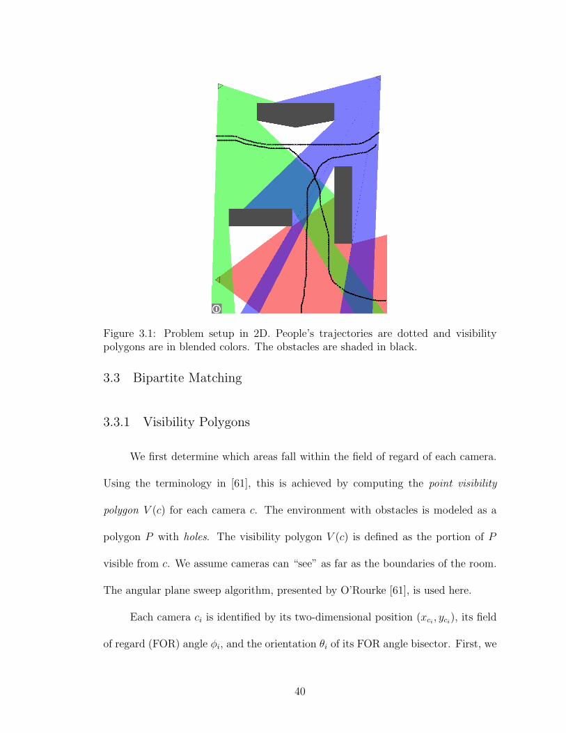
Figure 3.1: Problem setup in 2D. People’s trajectories are dotted and visibilitypolygons are in blended colors. The obstacles are shaded in black.
3.3 Bipartite Matching
3.3.1 Visibility Polygons
We first determine which areas fall within the field of regard of each camera.
Using the terminology in [61], this is achieved by computing the point visibility
polygon V (c) for each camera c. The environment with obstacles is modeled as a
polygon P with holes. The visibility polygon V (c) is defined as the portion of P
visible from c. We assume cameras can “see” as far as the boundaries of the room.
The angular plane sweep algorithm, presented by O’Rourke [61], is used here.
Each camera ci is identified by its two-dimensional position (xci, yci
), its field
of regard (FOR) angle φi, and the orientation θi of its FOR angle bisector. First, we
40
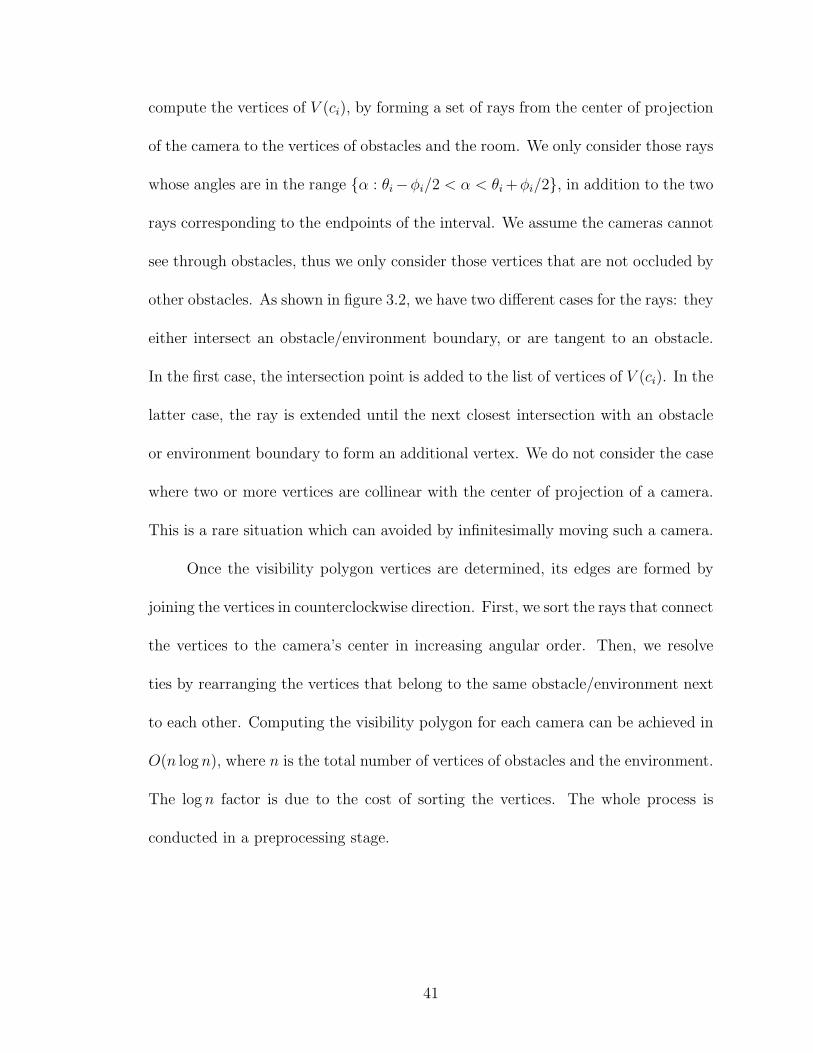
compute the vertices of V (ci), by forming a set of rays from the center of projection
of the camera to the vertices of obstacles and the room. We only consider those rays
whose angles are in the range {α : θi−φi/2 < α < θi +φi/2}, in addition to the two
rays corresponding to the endpoints of the interval. We assume the cameras cannot
see through obstacles, thus we only consider those vertices that are not occluded by
other obstacles. As shown in figure 3.2, we have two different cases for the rays: they
either intersect an obstacle/environment boundary, or are tangent to an obstacle.
In the first case, the intersection point is added to the list of vertices of V (ci). In the
latter case, the ray is extended until the next closest intersection with an obstacle
or environment boundary to form an additional vertex. We do not consider the case
where two or more vertices are collinear with the center of projection of a camera.
This is a rare situation which can avoided by infinitesimally moving such a camera.
Once the visibility polygon vertices are determined, its edges are formed by
joining the vertices in counterclockwise direction. First, we sort the rays that connect
the vertices to the camera’s center in increasing angular order. Then, we resolve
ties by rearranging the vertices that belong to the same obstacle/environment next
to each other. Computing the visibility polygon for each camera can be achieved in
O(n log n), where n is the total number of vertices of obstacles and the environment.
The log n factor is due to the cost of sorting the vertices. The whole process is
conducted in a preprocessing stage.
41
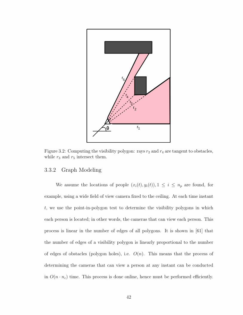
rr
r
r
r1
5
4
3
2
Figure 3.2: Computing the visibility polygon: rays r2 and r4 are tangent to obstacles,while r3 and r5 intersect them.
3.3.2 Graph Modeling
We assume the locations of people (xi(t), yi(t)), 1 ≤ i ≤ np are found, for
example, using a wide field of view camera fixed to the ceiling. At each time instant
t, we use the point-in-polygon test to determine the visibility polygons in which
each person is located; in other words, the cameras that can view each person. This
process is linear in the number of edges of all polygons. It is shown in [61] that
the number of edges of a visibility polygon is linearly proportional to the number
of edges of obstacles (polygon holes), i.e. O(n). This means that the process of
determining the cameras that can view a person at any instant can be conducted
in O(n · nc) time. This process is done online, hence must be performed efficiently.
42

k
di
occluded
shade angle
Figure 3.3: Computing occlusions of subjects by one another.
When the number of people np and the number of cameras nc are small, this can
be computed in O(n · nc · np) for all people, at each time instant. As np grows, a
more efficient approach is to divide the plane into cells that directly index visibility
polygons, and build a two-dimensional data structure that efficiently assigns people
to cells. An offline preprocessing stage will determine which cameras can view each
cell.
We also suggest a 2D model for the occlusion of people by one another with
respect to each camera. To compute the occlusion, we sort the subjects within each
visibility polygon w.r.t. the angles they make with their respective cameras. Then,
for each subject, we find its neighbors that are located farther from the camera, and
mark them as occluded. Given a camera, a subject S1 occludes a subject S2 if S1
is closer to that camera than S2, and S2 falls within the “shade” of S1. The shade
angle of a subject i is computed using the equation: αi = tan−1 k√d2
i−k2as shown in
figure 3.3.
Finally, we model the camera assignment problem as matching in a bipartite
graph G = ((V, U), E) as shown in figure 3.4. The vertices V represent the people
and U the set of cameras. An edge eij ∈ E, between vi and uj, exists if camera
cj can view person pi, that is pi falls inside the visibility polygon of cj and is not
43

occluded by another person. The problem is to match as many vertices as possible
from V (people) to vertices in U (cameras), with the constraint that each camera
is matched to at most one person. This is the classical bipartite matching problem
[20].
3.3.3 Initial Matching
Once the bipartite graph is constructed, we compute an initial matching. Fig-
ure 3.4 shows an example of a perfect matching, where all vertices are matched.
This is not always possible, and hence, we seek a maximum cardinality matching,
in which we try to match as many vertices as possible. Specifically, we are inter-
ested in matching as many vertices of V (people) as possible. This proceeds by
visiting each unmatched v-node, then using a modified breadth-first-search (BFS)
algorithm to reach the closest unmatched u-node, and finally matching both. The
BFS algorithm is modified so as to restrict visited edges to be sequences alternating
between matched and non-matched edges. These sequences are known as alternating
paths. When no more alternating paths can be found in the graph G, a maximum
matching is found. It is proved (see [62] for example) that a standard matching al-
gorithm (Edmonds’ [20]) correctly solves the matching problem for a bipartite graph
in O(min(|V |, |U |) · |E|). In practice, nc ≤ np, so the initial matching complexity is
O(n2c · np).
44

people cameras
u
u
u
u
v
v
v
v
1
4
3
2
1
2
3
4
matched edge
Figure 3.4: An example of the problem model with a perfect matching.
3.3.4 Matching Update
As people move through the room, their positions within the fields of regard of
cameras are updated. In the event that a person enters a visibility polygon, exits it,
becomes occluded or becomes visible, the change results in updating the bipartite
graph accordingly, and possibly recomputing the matching. There are four cases
here, depending on the type of graph update that has occurred:
• If no edges included in the matching, called matched edges, are removed, noth-
ing has to be done.
• If one or more matched edges are removed, we attempt to augment the match-
ing.
• If one or more edges are added to an incomplete matching, we attempt to
augment it.
• If one or more edges are added to a complete matching, nothing has to be
done.
45

The matching algorithm is incremental by nature. The cost of each stage is O(|E|) '
O(np ·nc). This property reduces significantly the running time of subsequent match-
ing computations, since practically, very few people change visibility regions at any
time, as will be shown in the results section. Depending on the type of graph update
that occurs, the search for an alternative matching proceeds as follows:
1. Determine a non-matched vertex v ∈ V (person).
2. Span a tree rooted at v using modified BFS.
3. If non-matched leaf nodes in U (cameras) are reached, choose the closest one
(u) to the tree root. The alternating path from v to u, forms the new aug-
mented matching.
4. If no leaf nodes exist which are non-matched vertices in U , we conclude that
v cannot be matched.
At each time, we only need to run this procedure for unmatched vertices. This
represents an order of magnitude time savings over solving the matching problem
for the entire graph at each update. In addition, matching the tree root to the
shallowest non-matched leaf guarantees that we obtain the minimum number of
re-assignments at each step. Figure 3.5 illustrates the two matching update cases
that involve edge removal, and figure 3.6 shows how an incomplete matching is
augmented when an edge is added.
46
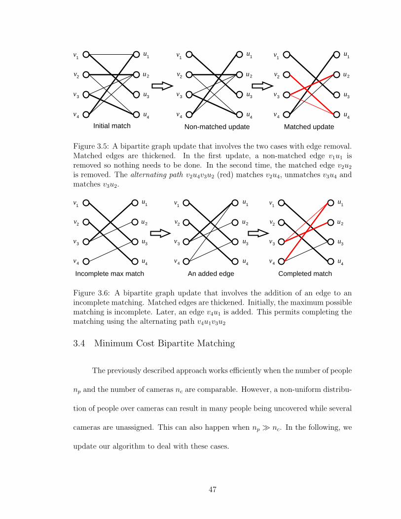
u
u
u
u
v
v
v
v
1
4
3
2
1
2
3
4
u
u
u
u
v
v
v
v
1
4
3
2
1
2
3
4
u
u
u
u
v
v
v
v
1
4
3
2
1
2
3
4
Initial match Non-matched update Matched update
Figure 3.5: A bipartite graph update that involves the two cases with edge removal.Matched edges are thickened. In the first update, a non-matched edge v1u1 isremoved so nothing needs to be done. In the second time, the matched edge v2u2
is removed. The alternating path v2u4v3u2 (red) matches v2u4, unmatches v3u4 andmatches v3u2.
u
u
u
u
v
v
v
v
1
4
3
2
1
2
3
4
u
u
u
u
v
v
v
v
1
4
3
2
1
2
3
4
u
u
u
u
v
v
v
v
1
4
3
2
1
2
3
4
Incomplete max match An added edge Completed match
Figure 3.6: A bipartite graph update that involves the addition of an edge to anincomplete matching. Matched edges are thickened. Initially, the maximum possiblematching is incomplete. Later, an edge v4u1 is added. This permits completing thematching using the alternating path v4u1v3u2
3.4 Minimum Cost Bipartite Matching
The previously described approach works efficiently when the number of people
np and the number of cameras nc are comparable. However, a non-uniform distribu-
tion of people over cameras can result in many people being uncovered while several
cameras are unassigned. This can also happen when np À nc. In the following, we
update our algorithm to deal with these cases.
47

3.4.1 People Grouping and Graph Modeling
The first step is to cover as many people as possible with a small number of
groups, where each group is represented by a disk on the ground plane that covers
the group. We constrain the groups (i.e. disks) to be of a small fixed size, since
covering a large group would generally require a significant zoom-out, which would
result in a video of low resolution. Such clustering problems are known to be NP-
hard, see, for example, [6]. Several variants of the problem we address have been
previously studied. In particular, Gonzalez [28] and Agarwal [6] suggest an O(n√
k)-
algorithm for the very similar problem of covering n points with fixed size squares,
where k is the number of required clusters. This is impractical in most situations,
such as ours. The authors also develop an approximate (not optimal) algorithm,
that runs in O(n log k).
We employ a greedy approximate algorithm, that starts with the group (disk)
that covers the maximum number of people, then the group with the next highest
cardinality, and so on. This is done as follows (see figure 3.7):
1. Center a disk over each person. This represents the locus of centers of disks
(groups) that can cover that person.
2. The plane is discretized using a grid, with its cells’ values incremented by one
for each disk that overlaps them.
3. Considering the disks in arbitrary order, if the next disk overlaps a previ-
ous one, the cardinalities of the grid cells forming the intersection region are
incremented and the cells are inserted into a priority queue.
48

1
1
1
1
1
1
2
2 2
2
3
A
A
A1
2
3
Figure 3.7: The approach used to cluster people. The cardinalities of the intersec-tions are marked to the left and the actual clusters to the right.
4. Dequeue a grid cell; it has maximum cardinality, say K.
5. Delete the K nearest subjects, assign them to a group, then remove the cor-
responding disks, decrementing the values of the involved grid cells.
6. Repeat 4) and 5) until only the grid cells with cardinalities 1 remain.
With np people and k clusters, this method requires O(np) insertions in the priority
queue, hence a complexity of O(np log k).
Once the clusters are formed, we model the problem as previously using a
bipartite graph G = ((V, U), E), with V here representing groups of people Ai
(possibly consisting of a single person) and U still representing the set of cameras.
An edge eij ∈ E, between vi and uj, exists if camera cj can view the group Ai.
A special case exists when a group falls on the edge of a camera’s visibility
region or when some of its people are occluded by others. In that case, no sin-
gle camera can view all the people of that group, which defeats the purpose that
grouping was originally developed for. We identify when this happens, then, using
a variant of the grouping algorithm, the formed groups are split, into the largest
49

subgroup that can be viewed entirely by a single camera, then the next largest,
and so on. Our experiments show that slight improvements in the coverage rate of
the algorithm is only achieved when the number of subjects is close to the number
of cameras. In what follows, we do not use the splitting variant of the grouping
algorithm.
3.4.2 Edge Weight Function
In order to view as many people as possible, priority is given to larger groups.
This is achieved by adding weights to the graph edges. The weighted bipartite
matching problem is that of finding a matching of G with the largest possible sum
of edge weights [62], or the minimum sum of costs. The problem was initially solved
by Kuhn [49] in O((|V | + |U |)3) time. Recently, an approximate algorithm that is
an order of magnitude faster has been suggested by Schwartz for edge weights that
satisfy certain properties [65].
To favor larger groups, we choose a cost function that assigns lower costs to
edges associated with larger groups and find a match with minimal cost. A typical
edge cost function is: cij = WMAX−wij, where wij is the number of people in group
i visible to camera j and WMAX is larger than any wij. We implement a variant
of Kuhn’s algorithm that is proven to find the optimal solution. The algorithm
proceeds by creating an auxiliary non-weighted graph which contains the minimum
cost edges incident on each node. Then, a maximum cardinality (non-weighted)
matching, similar to figure 3.4, is computed. If it is not complete, the next unused
50

minimum cost edge is added and an augmented matching, similar to figure 3.6,
is constructed. The process is repeated until all vertices of V (people) have been
matched, or no more edges remain. This method works only with complete graphs
that have |V | = |U |. This is achieved by completing the missing edges with ones
with costs WMAX , so they are not chosen during the optimization.
The use of a cost function that favors large groups of people results in small
groups and individual people to be unmatched to any camera for extended periods
of time. To balance the amounts of time each subject is covered, we add a time
penalty to the edge cost function. The updated cost function is:
cij = WMAX − wij − f(Ti) (3.1)
where, for each person, a variable Ti accumulates the amount of time that person
has not been assigned to any camera. For groups, we find the minimum positive
Ti of its members. Our experiments have shown that using the maximum Ti in
groups increases camera switches which produces a non-smooth video. At given
time thresholds, the cost of an edge changes due to the time penalty, and the cam-
eras are forced to switch. As a camera assignment changes, the variables Ti also
change, which might reverse a previous assignment immediately, causing an infi-
nite oscillation of cameras between two subjects. The function f(·) in equation
(3.1) above is just used to prevent this from occurring, keeping the camera switches
smooth. Similarly, other factors can also be included into the cost function, such as
the orientation of a person w.r.t. camera, where a person facing a camera will have
preference (lower cost) over a person facing away from it.
51

3.4.3 Matching Update
The changes occurring in groups, as people move through the environment, are
more involved than in the one-to-one case presented earlier. We present below how
these changes affect the graph topology, and how we efficiently update the solution.
3.4.3.1 Change in weights only, same graph topology
If a matching edge cost increases or a non-matching edge cost decreases, aug-
menting the solution is attempted. First, the match of the incident node is removed.
Then, a tree rooted at this node is spanned using the modified BFS as previously.
The branches of this tree are the potential alternating pathes. Along each path,
the cost of an undone matching edge is subtracted, while the cost of a newly added
matching edge is added. If a negative path is found, it means that we can find
a smaller cost matching. The smallest cost branch is then used to augment the
solution. If no negative paths are found, no better solution can be obtained.
If a matching edge cost decreases, nothing needs to be done. The intuition here
is that the cost was already minimal using that edge. Now, it’s even less. Similarly,
if a non-matching edge cost increases, no new solution needs to be searched for.
The current minimum cost solution did not use that edge and so obviously a new
solution won’t, when its cost has increased.
52

3.4.3.2 Change in graph topology
If an edge is added, this is equivalent to a cost decrease (from ∞ to c) of a
non-matching edge. If an edge is removed, this is equivalent to an edge cost increase
(from c to ∞): if it were a non-matching edge nothing has to be done, while if it
were matching, an augmented solution is constructed. Finally, adding/removing a
node to/from the graph (e.g., group split/merge) amounts to adding/removing at
most nc edges.
3.4.3.3 Time requirements
Since the solution is augmented here also using a modified BFS, the time
complexity of each update is similarly O(|E|) ' O(np·nc). When we have many more
people than cameras (np À nc), nc can be considered a constant, and the update
process is linear in the number of people np. By adding up the complexities of all the
components of our algorithm, we can see that the bottleneck is in grouping people
O(np log k). This represents the overall asymptotic complexity of the algorithm, if
grouping is required. If not required, the overall complexity is linear in np.
3.5 Implementation and Results
To evaluate our method under different conditions, we constructed a simula-
tor and, in addition, used the simulator developed by van den Berg et al. [73]. In
our simulator, obstacles’ locations and people’s trajectories and velocities are man-
ually traced. This enables more realistic agents’ trajectories. We have simulated
53
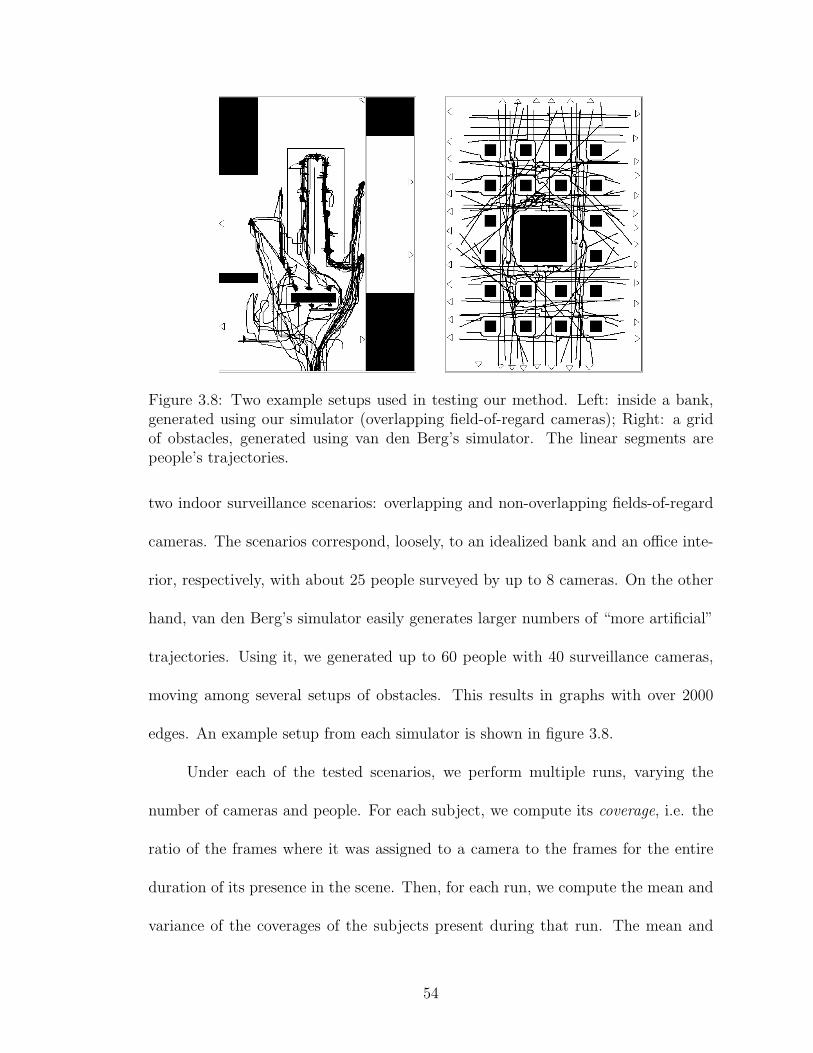
Figure 3.8: Two example setups used in testing our method. Left: inside a bank,generated using our simulator (overlapping field-of-regard cameras); Right: a gridof obstacles, generated using van den Berg’s simulator. The linear segments arepeople’s trajectories.
two indoor surveillance scenarios: overlapping and non-overlapping fields-of-regard
cameras. The scenarios correspond, loosely, to an idealized bank and an office inte-
rior, respectively, with about 25 people surveyed by up to 8 cameras. On the other
hand, van den Berg’s simulator easily generates larger numbers of “more artificial”
trajectories. Using it, we generated up to 60 people with 40 surveillance cameras,
moving among several setups of obstacles. This results in graphs with over 2000
edges. An example setup from each simulator is shown in figure 3.8.
Under each of the tested scenarios, we perform multiple runs, varying the
number of cameras and people. For each subject, we compute its coverage, i.e. the
ratio of the frames where it was assigned to a camera to the frames for the entire
duration of its presence in the scene. Then, for each run, we compute the mean and
variance of the coverages of the subjects present during that run. The mean and
54

variance are weighted by the subjects’ trajectory lengths.
Figure 3.9 shows the mean of the coverage for the two setups of figure 3.8, under
different grouping strategies, as the number of people and cameras vary. Group
diameters are measured in units of people’s average sizes. In the bank environment
(top), increasing the group size has a significant effect on coverage. The large amount
of open space enables this to happen. However, in the obstacles grid environment
(bottom), coverage increases with group size at a slower rate, because the narrow
“hallways” that exist between obstacles do not allow the formation of large groups.
Adding a time penalty to the edge cost function, as mentioned in equation
(3.1), distributes the coverage more evenly amongst the people who haven’t been
tracked in a while. We have experimented with different group sizes, in multiple
environments and with different problem sizes (number of people, cameras). As ex-
pected, adding the time penalty to the cost function reduces the standard deviation
of the coverage, due to a more even distribution. The standard deviation is further
reduced when there is a much greater number of people than cameras. This is be-
cause in these situations, and in the absence of a time penalty, the cameras tend
to remain assigned to the same subset of people to reduce camera switches, rather
than rotating to different people. Sample results for the two example setups are
shown in figure 3.10. We must note however that the matching algorithm already
produces the optimal result with respect to the mean of coverage. Thus, adding a
penalty term to obtain a more even distribution of coverage also results in a less
than optimal mean. We choose our penalty term carefully to balance between the
desired reduction in standard deviation and the undesired reduction in mean. In
55
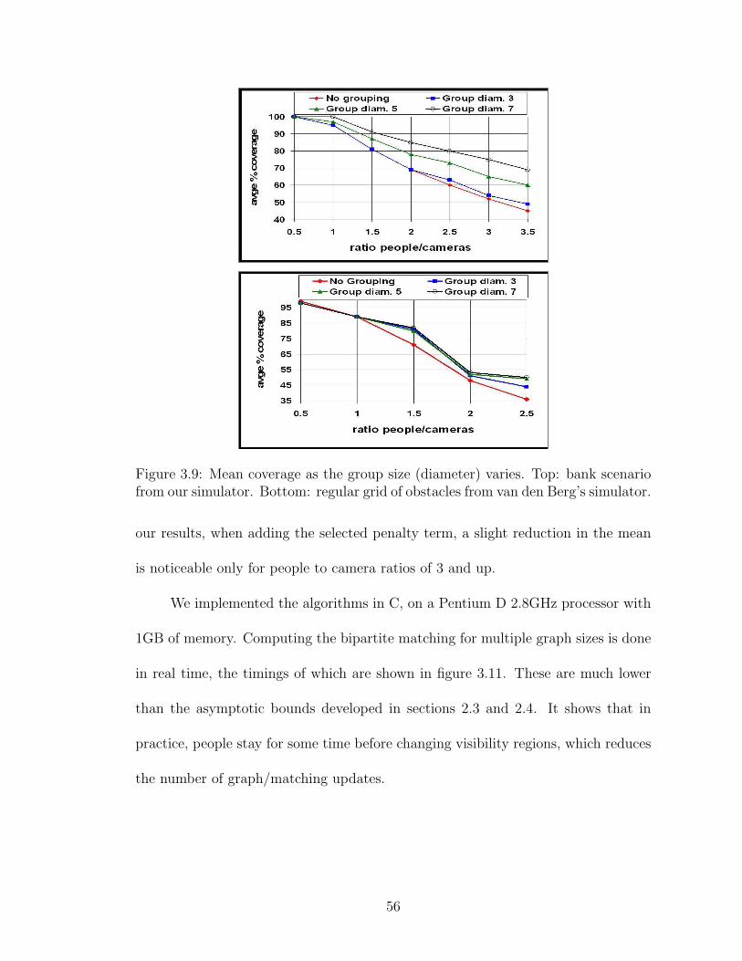
Figure 3.9: Mean coverage as the group size (diameter) varies. Top: bank scenariofrom our simulator. Bottom: regular grid of obstacles from van den Berg’s simulator.
our results, when adding the selected penalty term, a slight reduction in the mean
is noticeable only for people to camera ratios of 3 and up.
We implemented the algorithms in C, on a Pentium D 2.8GHz processor with
1GB of memory. Computing the bipartite matching for multiple graph sizes is done
in real time, the timings of which are shown in figure 3.11. These are much lower
than the asymptotic bounds developed in sections 2.3 and 2.4. It shows that in
practice, people stay for some time before changing visibility regions, which reduces
the number of graph/matching updates.
56
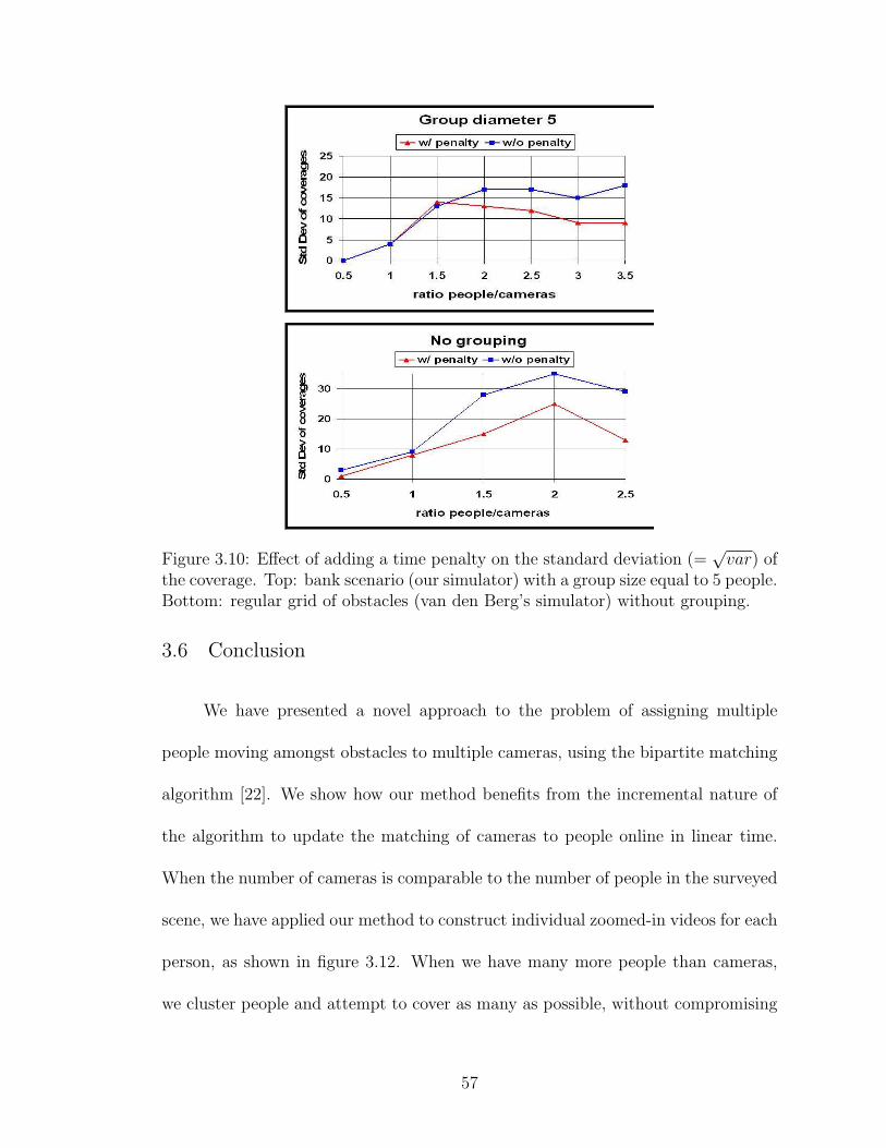
Figure 3.10: Effect of adding a time penalty on the standard deviation (=√
var) ofthe coverage. Top: bank scenario (our simulator) with a group size equal to 5 people.Bottom: regular grid of obstacles (van den Berg’s simulator) without grouping.
3.6 Conclusion
We have presented a novel approach to the problem of assigning multiple
people moving amongst obstacles to multiple cameras, using the bipartite matching
algorithm [22]. We show how our method benefits from the incremental nature of
the algorithm to update the matching of cameras to people online in linear time.
When the number of cameras is comparable to the number of people in the surveyed
scene, we have applied our method to construct individual zoomed-in videos for each
person, as shown in figure 3.12. When we have many more people than cameras,
we cluster people and attempt to cover as many as possible, without compromising
57
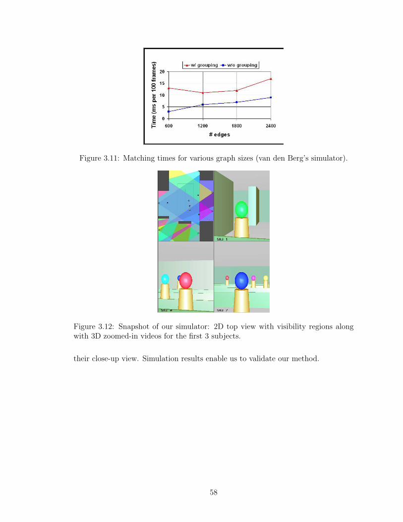
Figure 3.11: Matching times for various graph sizes (van den Berg’s simulator).
Figure 3.12: Snapshot of our simulator: 2D top view with visibility regions alongwith 3D zoomed-in videos for the first 3 subjects.
their close-up view. Simulation results enable us to validate our method.
58

Chapter 4
A Two-Player Pursuit-Evasion Game
4.1 Introduction
Finding subjects in environments with obstacles and keeping them under watch
is a problem that has many interesting surveillance and safety applications. In the
area of providing care for the elderly and disabled, tracking subjects is a prereq-
uisite to recognizing human activities, thus providing a safer home for the aged
(for example [19]). Intent recognition based on following an agent and knowing the
environment obstacles’ geometry has been the subject of study in [57].
4.1.1 Related Work
In the area of surveillance and security, in which we are more interested, the
moving subject can either be an intruder [45], [47], [44] an evader [84], [59], [9],
or simply a moving target that is to be put under watch. We also note that the
term target tracking is commonly used in the robotics literature (for example [36])
to mean maintaining the visibility of that target. We will stick to that terminology
in the rest of this thesis. The broad class of surveillance applications span several
interesting problems:
• Preventive art gallery problems, where the task is to find the optimal sensor
layout that prevents intrusions into the surveyed scene. The sensors can either
59

be fixed [61] or moving (mounted on robots) [44].
• Graph clearing problems that try to solve for the optimal number of robots
needed to verify that an environment with obstacles is free from intruders
(decontaminated) and that it will not get recontaminated [45], [47], [46], [48].
• Searching environments for initially invisible intruders/evaders. The passive
problem [84] estimates the approximate hiding locations of intruders and their
numbers, while the active problem decides how to move the robots to search
the environment [50].
• Tracking initially visible evaders, maintaining their visibility at all times, if
possible [10], [11], or maximizing the time they are visible, otherwise [9].
We elaborate here on the fourth application above, the pursuit evasion game,
since it is the most closely related one to our work. In two-player games, when the
layout of the environment’s obstacles is unknown [29], [9], the pursuer collects mea-
surements to determine the locations of the local obstacles. Based on the visibility
from its current position, the pursuer then determines the instantaneous next step
to take in order to increase the evader’s escape time. The algorithm proceeds in a
greedy manner to maximize the total time the evader is seen by the pursuer. Most
of the work in the area of maintaining the visibility of evaders has been done in 2D
although some attempts have been made in 3D as well [8].
When the number of players increases, the game becomes more complex.
Vieira et al. [76] solve the problem of finding the optimal time for multiple pur-
suers to capture multiple evaders. The complexity is exponential in the number of
60

players. They also present a partition of the game into multi-pursuer single-evader
games for a faster but near-optimal solution [77]. Another variation of the game is
to combine it with the intruder search problem into one model, as suggested in [36].
A large amount of literature has been devoted to two-player pursuit evasion
games, where one pursuer maintains the visibility of one evader, in an environment
with obstacles with known layout. Bhattacharya et al. address that problem, with
the additional condition that the pursuer loses the game immediately if it loses
sight of the evader at any time. As in [9], the authors also assume here that the
pursuer has complete information about the instantaneous position and velocity
of the evader. Under these conditions, the authors solve the decidability problem
around one corner [10]. The problem is said to be decidable if the outcome of the
game can be known for any initial positions of the pursuer and evader. However,
solving around one corner (i.e. two infinite edges meeting at a point) is restrictive;
there is no geometry “behind” which the evader can hide. The authors then extend
their work in [11] to deal with more general environments with convex obstacles.
However, in those environments, they are only able to provide a partial solution
to the decidability problem. They provide a sufficient condition for escape of the
evader. In other words, they find a region of initial positions, such that if the pursuer
lies outside it, the evader escapes for sure. However, if the pursuer lies inside that
region, the result of the game is undecidable. Their algorithm splits the environment
into regions that depend on the geometry of the obstacles.
Under the same earlier setup, Murrieta-Cid et al. [60] develop a tracking strat-
egy also by creating a partitioning of the environment that depends on the geome-
61

try of obstacles. Later, they present a more simple convex partitioning [59] that is
modeled as a mutual visibility graph. Their algorithm alternates between an evader
assumed to take the shortest step to escape, countered by a pursuer that computes a
prevention-from-escape step. The assumption of the evader taking the shortest step
to an escape region is a reasonable one, since if the pursuer is able to counter it, then
it will be able to counter any longer steps. However, this strategy is only locally
optimal. The authors thus find all possible permutations of escape sequences along
with corresponding prevention-from-escape steps. The global solution concatenates
adjacent “partial local paths”. This leads to an interesting result: To decide which
player wins, every feasible ordering of local paths has to be checked. The authors
reduce the traveling salesman problem to the current problem, concluding it is NP-
complete.
4.1.2 Contributions
Motivated by the work in [10], [11] and [59], we propose a novel algorithm to
determine the outcome of the tracking problem. Our approach relies on partitioning
the surveyed environment into a uniform grid that is independent of the geometry
of the obstacles. At each time instant, players can move one or more grid cells away,
according to their speeds. Given any initial pair of positions for the pursuer and
the evader, we provide a complete solution to the problem of deciding which player
wins in a computationally feasible time. In addition, if it is decided that the pursuer
wins, i.e. it is able to maintain visibility of the evader at all times, we also find its
62

optimal trajectory that always keeps the evader as far as possible from positions
from which it can escape. We are currently exploring the effect of varying the grid
cells’ size on the accuracy of the results and the efficiency of computing them.
In the rest of this chapter, we proceed with a more detailed definition of
the problem in section 4.2, followed by a couple of examples that illustrate the
construction of our algorithm in section 4.3. Then, we detail our approach more
formally in section 4.4. Finally, we suggest future work on this problem in section
4.5.
4.2 Problem Definition
Several variants of the pursuit evasion problem have been attempted. In this
work, we are interested in a setup similar to that in [11] and [59]. In what follows,
we present in detail the environment setup and the conditions on the players.
4.2.1 Environment Layout and Rules of the Game
We will deal here with indoors environments that contain obstacles that ob-
struct the view of the players. In the 2D domain which we are solving, the obstacles
are represented as polygons with known geometries and locations. This is a two-
player game, with one pursuer and one evader represented as points. Each player
knows exactly both the position and velocity of the other player. Both players move
at bounded speeds and can maneuver to avoid obstacles. They are equipped with
sensors that can “see” in all directions (ommnidirectional) and as far as the envi-
63

ronment boundaries or obstacles, whichever is closer. We will see later than we can
restrict this property with a simple variation in our algorithm.
The pursuit evasion game proceeds as follows. Initially, the pursuer and the
evader are at positions from which they can see each other. As in [11], we define
two players to be visible to one another if the line segment that joins them does
not intersect any obstacle. The goal of the game is for the pursuer to maintain the
visibility of the evader at all times. The game ends immediately, if at any time, the
pursuer loses sight of the evader. In that case, we say that the pursuer loses and
the evader wins.
4.2.2 Space Discretization
The key idea in our algorithm is our space partitioning method. Unlike earlier
work ([11], [59]), our partitioning does not depend on the geometry of the envi-
ronment and obstacles. Instead, it depends on the motion of the players. Using a
time-discretization similar to [9], we consider the positions of each player at time
intervals of ∆t units. If the velocity of a player at a certain time interval is v, the
distance traveled during the discrete time step will be ∆d = v∆t. We recall that
the players’ velocities are bounded and, by the same token, can also be discretized
as 0, vmin, . . . , vmax. We thus choose to partition the space into a uniform grid with
cell edge length:
l = vmin∆t. (4.1)
64
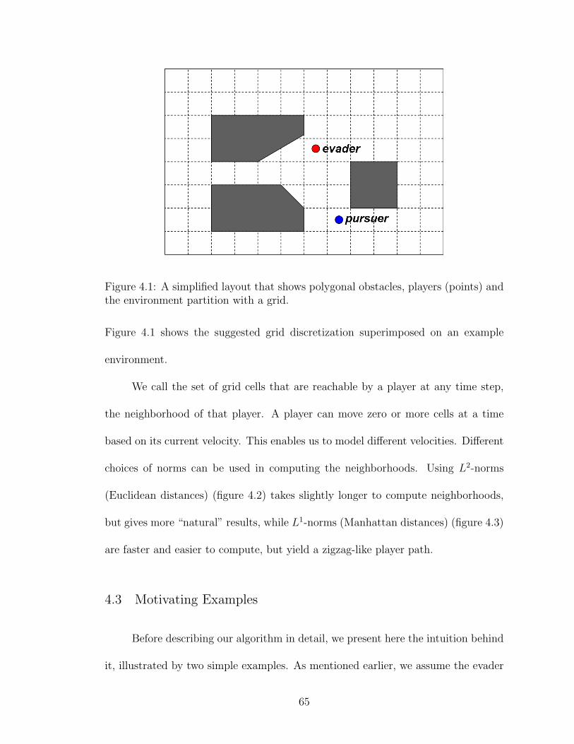
Figure 4.1: A simplified layout that shows polygonal obstacles, players (points) andthe environment partition with a grid.
Figure 4.1 shows the suggested grid discretization superimposed on an example
environment.
We call the set of grid cells that are reachable by a player at any time step,
the neighborhood of that player. A player can move zero or more cells at a time
based on its current velocity. This enables us to model different velocities. Different
choices of norms can be used in computing the neighborhoods. Using L2-norms
(Euclidean distances) (figure 4.2) takes slightly longer to compute neighborhoods,
but gives more “natural” results, while L1-norms (Manhattan distances) (figure 4.3)
are faster and easier to compute, but yield a zigzag-like player path.
4.3 Motivating Examples
Before describing our algorithm in detail, we present here the intuition behind
it, illustrated by two simple examples. As mentioned earlier, we assume the evader
65
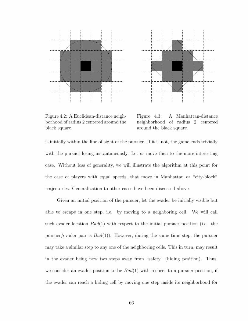
Figure 4.2: A Euclidean-distance neigh-borhood of radius 2 centered around theblack square.
Figure 4.3: A Manhattan-distanceneighborhood of radius 2 centeredaround the black square.
is initially within the line of sight of the pursuer. If it is not, the game ends trivially
with the pursuer losing instantaneously. Let us move then to the more interesting
case. Without loss of generality, we will illustrate the algorithm at this point for
the case of players with equal speeds, that move in Manhattan or “city-block”
trajectories. Generalization to other cases have been discussed above.
Given an initial position of the pursuer, let the evader be initially visible but
able to escape in one step, i.e. by moving to a neighboring cell. We will call
such evader location Bad(1) with respect to the initial pursuer position (i.e. the
pursuer/evader pair is Bad(1)). However, during the same time step, the pursuer
may take a similar step to any one of the neighboring cells. This in turn, may result
in the evader being now two steps away from “safety” (hiding position). Thus,
we consider an evader position to be Bad(1) with respect to a pursuer position, if
the evader can reach a hiding cell by moving one step inside its neighborhood for
66

whichever neighboring cell the pursuer is able to move to. Inductively, we call a
location Bad(2) if it satisfies the same above conditions but with respect to Bad(1)
locations. We have shown the intuition here for a single initial position. We note,
however, that we cannot begin labeling any Bad(2) cell until we have computed all
the Bad(1) maps for every initial position of the evader. This guarantees that all
the possible pursuer-evader location pairs are considered. We stop the search when
either of these two conditions is met:
1. All the environment cells are labeled Bad(x) for some finite value of x. This
means that there is no winning strategy for the pursuer starting from its initial
position.
2. We reach a state where Bad(i + 1) = Bad(i) for all labeled cells, with some
cells non-labeled. This means that if the evader is initially located outside of
these cells, it will never be able to go out of sight of the pursuer.
4.3.1 A “Level-0” Game
We illustrate our method first with the example shown in figure 4.4. We
consider a simple partition where a grid cell is as big as an obstacle. We defer to a
later point the analysis of how different grid cell sizes can affect the solution. In this
model, we define two cells to be visible to one another if the line segment from their
centers does not intersect an obstacle. If the line segment is tangent to an obstacle,
we still consider the cells to be visible to one other. Other visibility models can be
substituted as desired. Given equal and constant speeds for both players, it is clear
67
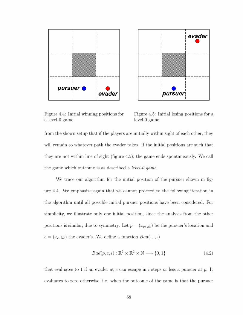
Figure 4.4: Initial winning positions fora level-0 game.
Figure 4.5: Initial losing positions for alevel-0 game.
from the shown setup that if the players are initially within sight of each other, they
will remain so whatever path the evader takes. If the initial positions are such that
they are not within line of sight (figure 4.5), the game ends spontaneously. We call
the game which outcome is as described a level-0 game.
We trace our algorithm for the initial position of the pursuer shown in fig-
ure 4.4. We emphasize again that we cannot proceed to the following iteration in
the algorithm until all possible initial pursuer positions have been considered. For
simplicity, we illustrate only one initial position, since the analysis from the other
positions is similar, due to symmetry. Let p = (xp, yp) be the pursuer’s location and
e = (xe, ye) the evader’s. We define a function Bad(·, ·, ·)
Bad(p, e, i) : R2 × R2 × N −→ {0, 1} (4.2)
that evaluates to 1 if an evader at e can escape in i steps or less a pursuer at p. It
evaluates to zero otherwise, i.e. when the outcome of the game is that the pursuer
68

Figure 4.6: Computing the labeling function Bad(N(p), e, 0) for the neighborhoodof a pursuer located at position p, where p′ and p′′ are the only possible neighborsfor p due to the obstacle.
wins. Our goal is to compute Bad(p, e, i) for all p and e.
When i = 0, Bad(p, e, 0) = 1 for all pairs of cells (p, e) mutually non-visible.
As elaborated earlier, given an initial (p, e) pair, we only consider the cells non-
visible from all of the positions neighboring the pursuer’s initial position. This is
denoted as Bad(N(p), e, 0) where N(p) is the neighborhood of p. It is computed
as the disjunction of the values Bad(p′, e, 0) for all p′ in the neighborhood of p.
Figure 4.6 illustrates this step. The notation in the figure might be confusing at
first. To make the notation easier and illustrate the tracing of the algorithm at each
iteration i, we choose a single pursuer position p, then label i all the cells for which
Bad(p, e, i) = 1. The other cells for which Bad(p, e, i) = 0 are just left blank.
The next step is to find all the positions that can reach, in at most one time
step, a cell of Bad(N(p), e, 0). An evader in any such position is able to win in
no more than one step. Using our definition (equation 4.2), these positions are
denoted Bad(p, e, 1) and labeled by 1’s in figure 4.7. At that point, we notice
that Bad(p, e, 1) = Bad(p, e, 0). That means that after one time step, and for
all possible pairs of moves that either player can make, the set of cells that were
69

Figure 4.7: Extending Bad(N(p), e, 0) into Bad(p, e, 1). Steady state is reached atthat point.
initially non-visible to the pursuer (escape cells) cannot be modified. This indicates
that the outcome of the game cannot be modified in favor of either player. When
we reach that state, we conclude that an evader in any labeled cell wins (in this case
instantaneously), and loses if in any other cell. We call this a steady state.
More formally, Bad(p, e, 1) can be expressed in terms of Bad(p, e, 0) using the
following recursive equation:
Bad(p, e, 1) = 1 ∀(p, e) : ∃e′ ∈ N(e)
s.t. Bad(p′, e′, 0) = 1 ∀p′ ∈ N(p).
(4.3)
Since N(e) and N(p) contain both e and p, Bad(p, e, 1) = 1 for all the pairs (p, e)
for which Bad(p, e, 0) = 1.
4.3.2 A “Level-1” Game
We now show an example of a game that reaches steady state after two
“rounds” or iterations, namely a level-1 game. The setup used in this game is
the one shown in figure 4.8. In this setup, it can be easily identified that if the
evader is 1 or 2 cells ahead of the pursuer, it can never escape. Otherwise (3 or
more cells ahead), the evader can break the line of sight and win.
70
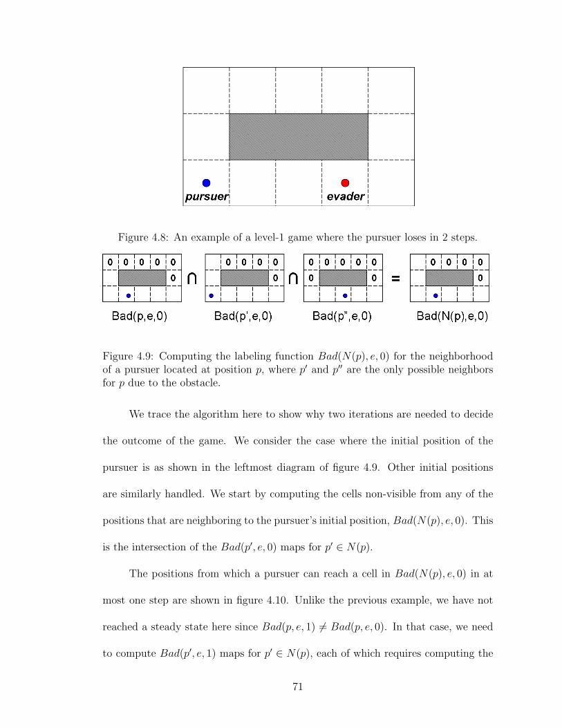
Figure 4.8: An example of a level-1 game where the pursuer loses in 2 steps.
Figure 4.9: Computing the labeling function Bad(N(p), e, 0) for the neighborhoodof a pursuer located at position p, where p′ and p′′ are the only possible neighborsfor p due to the obstacle.
We trace the algorithm here to show why two iterations are needed to decide
the outcome of the game. We consider the case where the initial position of the
pursuer is as shown in the leftmost diagram of figure 4.9. Other initial positions
are similarly handled. We start by computing the cells non-visible from any of the
positions that are neighboring to the pursuer’s initial position, Bad(N(p), e, 0). This
is the intersection of the Bad(p′, e, 0) maps for p′ ∈ N(p).
The positions from which a pursuer can reach a cell in Bad(N(p), e, 0) in at
most one step are shown in figure 4.10. Unlike the previous example, we have not
reached a steady state here since Bad(p, e, 1) 6= Bad(p, e, 0). In that case, we need
to compute Bad(p′, e, 1) maps for p′ ∈ N(p), each of which requires computing the
71

Figure 4.10: Extending Bad(N(p), e, 0) into Bad(p, e, 1).
Figure 4.11: Computing the labeling function Bad(N(p), e, 1) out of the mapsBad(pi, e, 1) for neighbors of position p.
corresponding Bad(pi, e, 0) maps. Recall that Bad(N(p), e, 1) is the disjunction of
the values Bad(p′, e, 1) for all p′ in the neighborhood of p. The process is shown in
figure 4.11.
We start the third iteration by finding all the positions that can reach a cell
in Bad(p, e, 1) in at most one step, namely Bad(p, e, 2) (figure 4.12). Here, we have
Bad(p, e, 2) = Bad(p, e, 1), meaning that two time steps after the initial start time
do not make more “escape” cells available to the evader than one time step. We
thus break the iteration at that point and conclude we reached steady state. Any
evader initially in a labeled cell has some way of escaping. We also see in figure 4.12
that “bad” cells are indeed three or more cells away of the pursuer’s initial position,
as intuitively guessed. At this point, we generalize the recursive equation 4.3 for
72

Figure 4.12: Extending Bad(N(p), e, 1) into Bad(p, e, 2). Steady state is reached atthat point.
any iteration.
Bad(p, e, i + 1) = 1 ∀(p, e) : ∃e′ ∈ N(e)
s.t. Bad(p′, e′, i) = 1 ∀p′ ∈ N(p).
(4.4)
Once the cells are classified as either “bad” or “non-bad”, for every initial
position that the pursuer can be in, we have a complete answer to the question of
deciding which player wins. However, we can use the information we have already
computed to determine the optimal tracking strategy that the pursuer should follow.
By labeling every non-bad cell with its distance to the closest bad cell (i.e. shortest
escape path), the goal of the pursuer is to choose its next step so that the associated
map has the evader in a non-bad cell with largest label.
4.4 Game Result and Tracking Strategy
We present here the formal algorithm for determining the existence of a win-
ning strategy for the pursuer. Along the way, we construct visibility maps that
determine partial solutions. Once the algorithm terminates, we show how we can
use the final visibility map to construct the actual winning strategy, if one exists.
We prove the correctness of our algorithm and provide bounds for its space and time
73

complexity.
4.4.1 Algorithm
Algorithm 1 computes the visibility map of an environment that determines,
for every pair of cells, whether or not a winning strategy exists. In this algorithm,
neighboring cells are computing based on the distance norm that is used. In addition,
a cell is not considered part of a neighborhood if it is occupied by an obstacle.
Algorithm 1. Determine if a winning strategy exists.
Input: Environment with obstacles coordinates.Output: A matrix that determines for every pair of locations whether a winningstrategy exists.Data Structure: Two N ×N matrices M and M’.
1. Partition the environment into a uniform grid of N cells.2. Initialize M and M’ to 0 matrices.3. for (0 ≤ p, e < N) Set M(p, e)=1 if cell e visible to cell p.4. finish=FALSE.repeat
5. for(0 ≤ p, e < N) M’(p, e) = ∩q M(q, e) ∀q ∈ Neighb(p).6. for(0 ≤ p, e < N) M’(q, e)=1 ∀q ∈ Neighb(p) s.t. M’(p, e)=1 ∧M’(q, e)=0.7. if (M’=M) thenfinish=TRUE else M=M’.
until finish=TRUE.
At the conclusion of the algorithm, if M(p, e)=1, the initial player positions
p and e are such there exists a strategy by which the evader can escape and the
pursuer loses. If M(p, e)=0, the evader can never escape and the pursuer wins.
To determine the tracking strategy in the latter case, we add this extension to the
previous algorithm.
74

i = 1.while (∃M(p, e) = 0)
Set M’(q, e) = i + 1 ∀q ∈ Neighb(p) s.t. M’(p, e) = i and M’(q, e)=0.i = i + 1.
end
4.4.2 Proof of Correctness
We first note that our algorithm always terminates. This happens either when
the visibility matrix does not get modified (M’=M) or when all the N cells are
labeled 1. Next, we prove the correctness of the algorithm by induction. At iteration
0 (step 3 of the algorithm), M does indeed contain the decision of the game, since
by definition, if M(p, e)=0, the pursuer cannot see the evader and the game ends,
and vice versa. Now, let the matrix M contain the outcome of the game at iteration
i. If M’ 6= M, it means that there exists a step that the evader can take to reach a
cell from which it can escape in i steps, i.e. an escape path of length i + 1. All such
steps are recorded in M’ which becomes the new decision matrix. However, if M’
= M, no additional step can improve the situation of the evader. It is useless to go
beyond, and we stop at that point.
4.4.3 Space and Time Complexity
Algorithm 1 requires two N × N matrices to store the temporary visibility
maps. This is O(N2) space requirements, where N is the number of cells in the
discretizing grid. With regards to time complexity, steps 3, 5, 6 and 7 are each
O(N2). We are interested in the three steps that occur inside the loop. The worst
case is to have all cells labeled. We argue here that this case will require O(N)
75

iterations, since each iteration labels one “layer” of O(N) cells around the current
labeled block, thus labeling the entire environment in O(N) iterations. This makes
the total time complexity O(N3).
4.5 Additional Work
We have presented the algorithm, verified its correctness and derived its poly-
nomial complexity. At this point, we need more extensive experiments with larger
environments. The simulators used in chapter 2 can also be used here for that pur-
pose. The main point that needs to be analyzed is to determine how the grid size
affects the results. We have just shown that the complexity of the problem depends
on the number of cells in the grid. It is thus desirable to reduce that number as
long as it does not affect the accuracy of the results. Consider a large cell size or
equivalently small number of cells. If the cell size is larger than some obstacles, the
accuracy of the visibility matrix is questionable.
We would like also to consider coalescing neighboring cells that share the same
visibility property. The cells will not physically disappear, since they represent the
step each player takes within a time unit. However, this can significantly reduce
redundant computations. We are motivated here by the work of [59] and the way
they partition the environment. Finally, some minor variations can also be consid-
ered when comparing the performance of the algorithm under different conditions.
We have already seen that the shape and size of the neighborhood model different
distance norms and players’ velocities respectively. We can also restrict players vis-
76

ibility, for example not “seeing” beyond a certain distance, by reducing the number
of labeled cells in the initial visibility matrix.
77
Chapter 5
Detecting Unusual Activity in Surveillance Video
5.1 Introduction
In this chapter, we present some older work that was done in the area of
anomaly detection. The research presented in this chapter is meant to fit within the
framework of the future control room introduced in chapter 2 (see figure 1.2). We
suggest a technique that can be used to “score” surveillance videos according to their
level of interest to human operators. Given the huge amount of available surveillance
video, it is necessary to filter video where little of interest occurs [34]. For this
purpose, we develop a video scoring technique based on modeling co-occurrence
statistics of moving objects. In particular, we identify unusual events as those rare
or non-frequent, according to a learned model.
Unlike previous work, special attention is given here to situations where each
agent’s behavior might not be independently unusual, but it is the joint occur-
rence that creates an unusual situation. This problem is solved by computing co-
occurrence statistics in both time and space, rather than just in time. To illustrate
the idea further, consider the example of two cars crossing simultaneously while
their trajectories intersect (figure 5.1). Each car’s trajectory would be considered
usual, had they crossed independently. Experiments are performed on synthetic
data, where time intervals and locations of unusual activities are reported. The less
78

Figure 5.1: Introductory example that shows the type of anomalies we are interestedin. The first two events are usual, but the third is not. Although it consists of acombination of exactly the two left event, it is their simultaneous occurrence thatmake it unusual
frequent an event is, the more unusual it becomes, and the higher the score assigned
to the involved video segment. Within the context of the display wall discussed in
chapter 1, the scores assigned to the videos are used, along with other constraints,
to control the mapping of videos to the display space. Higher score videos will be
assigned a larger area of the display wall, and a location that attracts more attention
of the operator.
The rest of this chapter is organized as follows: section 5.2 reviews in some
detail earlier work that has been done in the area of anomaly detection in video.
In section 5.3, we formally define the problem then present our approach to solving
it in section 5.4. We show results in section 5.5 then suggest future extensions in
section 5.6.
79

5.2 Literature review
5.2.1 Definition of “unusual events”
Much effort has been devoted to the area of activity recognition. However,
the problem of detecting generically interesting activity is still very much an open
problem [82]. Depending on the type of application and the approach employed,
interesting activity has been interchangeably called “abnormal activity” [19, 51,
75, 81, 82], “unusual activity” [39, 86], “atypical behavior” [54, 58], “inexplicable
behavior” [33, 34], and “anomalous activity” [31, 56]. We choose the term unusual
events to refer to non-frequent or rare ones.
To solve the problem of detecting unusual events, we must first give a definition
of that term. Human operators monitoring surveillance cameras might differ greatly
in their definition. They can be influenced more by people’s appearance than by
their behavior [34]. To avoid this bias, authors have based their definitions on the
model they choose to represent activity. Stauffer et al. [67] define unusual events
as those which have rarely or never occurred. Hung et al. [39] detect the least
frequent occurrences corresponding to peaks of salient motion. Vaswami et al. [75]
define abnormal activity (or suspicious behavior) as a slow or drastic change in a
model, whose parameters are unknown. Morris et al. [58] assume that low speed and
low distance to objects at trajectory landmarks are considered unusual. Dee et al.
[33, 34] consider those trajectories that do not proceed towards a goal as unusual.
Xiang et al. [81] define abnormality as behavior patterns that are not represented
by sufficient samples in a training dataset. Micheloni et al. [56] focus on the time
80

spent by an object in the observed scene, where “too long” or “too short” a time
needed to perform a specific activity would point to an anomalous event. Duong et
al. [19] also focus on state duration and not on state order for the model they use
for activity. Zhong et al. consider events (video segments) to be unusual if there are
no similar events. Liao et al. [18, 51] detect abnormal behaviors by noting when an
agent departs from a familiar routine by matching to a learned model. Hamid et
al. [31] assert that anomalous activity is rare and dissimilar from learned models of
regular activities.
5.2.2 Detecting unusual activity
Several approaches have been attempted to detect unusual activity in video.
Zhong et al. [86] used document clustering techniques with video segments as doc-
uments and prototype features as keywords. The clusters with small inter-cluster
similarity are considered unusual events, according to a developed similarity mea-
sure. This approach doesn’t model interactions between spatially separated objects.
It fits under the topic of anomaly detection, where the training data is clustered,
and “distant” objects identified as outliers [70].
Morris and Hogg present a simple statistical approach in [58]. They test their
approach on a scene with pedestrians interacting with cars parked in a parking lot.
With this scenario, they assume that low speed and low distance of pedestrians to
landmark points (parked cars, etc. . . ) are considered unusual. They form a model by
accumulating probabilities of speed and distance and test it on sample trajectories.
81

This model might be too restrictive to the specific application presented. Dee and
Hogg develop a measure of intentionality to filter surveillance data. Agents’ behavior
(humans) is modeled using a state transition diagram, with high costs on transitions
that lead to inexplicable goals. Low cost footage is removed, leaving only video that
is potentially interesting. It’s not clear how transition diagrams can be developed
to model different scenarios, but this work is actively pursued in [33, 34, 35].
Hamid et al. [31] use natural language processing techniques to detect and
explain anomalous activity in video. Activity is represented as histograms of event
n-grams. With a value of n chosen to be 3, this is equivalent to breaking the video
into overlapping chunks of 3 time units. Micheloni et al. [56] train an active event
database with observed simple events. Composite events are formed by arranging
simple events in a finite automaton. Finally, activities are timed and classified
unusual if their duration is too short or too long. Again, both of these methods
classify isolated events.
Co-occurrence statistics have been used differently in the literature. Stauffer
et al. [67] accumulate joint co-occurrences of codebook symbols to classify video
sequences. Co-occurrences are computed between pairs of symbols in the same
sequence; thus multiple-object interactions are not modeled. In addition, for large
codebooks, the method becomes inefficient with large co-occurrence matrices. More
recently, Ermis et al. [23] also use co-occurrence statistics, but after “subtracting”
normal motion patterns first. Hung and Gong overcome both these problems in [39].
First, salient features are extracted and their local spatio-temporal co-occurrences
are computed for each frame. Then, higher level spatial co-occurrences are computed
82

for the rate of change of the first ones. Finally, the least frequent occurrences define
the salient events, which correspond to unusual activity. It is not mentioned how
the choice of the time interval for local temporal correlations affects the results. The
authors have chosen a local temporal neighborhood of 3 frames and just noted that
it affects self correlations. It is also questionable how saliency of intensity affects
false alarms. For example, usual events of “opening the door” are detected as salient
due to the change in intensity.
Activity modeling and recognition has often been presented in the literature
in connection with Hidden Markov Models (HMM). In a nutshell, a dynamic model
is created for the usual activity. Later on, as new activity is presented to the
surveillance system, that activity which do not “fit” the model is considered unusual.
Unfortunately, such methods tend to behave poorly in scenes with complex activity,
when the number of usual activities is too high to model. A brief discussion is
presented in [19] and [86]. This has led to the development of many variants to the
basic HMM.
Makris and Ellis [54] present the basic HMM approach. For the method to
work properly, the scene is limited to pedestrian trajectories near the entrance of
a university building. Tracking is assumed perfect with trajectories represented as
sequences of nodes. Despite this “ideal” situation, the authors perform a slight
update by training their model for each time of the day, to accommodate variations
of pedestrian behavior. The trained model is presented with trajectories for which
it computes the likelihood of belonging to a trained model, and detects the node on
the path which departs from that model. Hu et al. [37] build a statistical model for
83

trajectory clusters which they call motion patterns. The distribution parameters for
each motion pattern are evaluated using maximum likelihood. Then, a probability
of anomaly occurrence is computed for partial and complete trajectories. In their
results, the authors show current abnormality probabilities beside tracked moving
objects.
Xiang and Gong [81] use an HMM variant, the Multi-Observation HMM, to
model behavior pattern. Then, an affinity matrix is formed for spectral clustering
of the data. Abnormal behavior has a low probability of belonging to any cluster.
The authors develop this approach further in [82] by noting that patterns initially
considered to be abnormal might later fit in the model as it is updated live. Duong et
al. introduce the Switching Hidden Semi-Markov Model (S-HSMM) in [19]. Since
they address the problem of learning human activities of daily living, they limit
abnormality detection to state duration rather than state order. Liao et al. address
the same problem also. In [51], the approach is based on modeling agents locations
(obtained through GPS sensor measurements) using a hierarchical Markov model.
All these applications are focused on single object trajectory modeling rather than
object interaction.
Vaswami et al. represent observed objects as configurations of point-object
locations known as shapes [75]. The problem thus becomes that of modeling the
shape motion and deformation using a continuous-state HMM, that the authors call
“shape activity”. Two measures are developed for drastic change and slow change
in the system model, which are chosen to signal abnormal activity. This includes
object interactions as well as time modeling. The authors present two methods to
84

solve the problem of varying the number of point-objects in shapes over time. It’s
not clear, however, how the system would perform in scenes where this is a frequent
situation. A simple example is that of a traffic intersection, where the observed
window is constantly having objects appearing and others leaving the scene. Such
situation would consume most of the system’s time in “resampling” shapes.
5.3 Problem definition
Our goal is to develop a method to detect unusual events in video, that can
adapt easily and quickly to various scenes. Our main contribution is in modeling
activity, which involves the interaction between multiple objects. In particular, we
are interested in situations where individual objects activities might be usual, while
their simultaneous occurrence is unusual.
Most earlier work has avoided co-occurrence statistics methods due to their
high complexity. Instead, researchers attempted to detect abnormality by building
and training models for the observed activity, such as HMM and variants. However,
these approaches have been limited to specific applications or scenes (e.g. ADL
[19, 51]). In some cases, human made rules for defining goals and intentions had to
be injected in the model [33].
We propose a representation of video data that reduces the expensive compu-
tations inherent in the co-occurrences approach. As in [82], we propose to update
the statistics online. In this case, an event that was initially classified as unusual due
to the lack of training data, might eventually prove to be usual as similar patterns
85
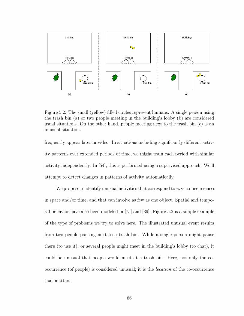
Figure 5.2: The small (yellow) filled circles represent humans. A single person usingthe trash bin (a) or two people meeting in the building’s lobby (b) are consideredusual situations. On the other hand, people meeting next to the trash bin (c) is anunusual situation.
frequently appear later in video. In situations including significantly different activ-
ity patterns over extended periods of time, we might train each period with similar
activity independently. In [54], this is performed using a supervised approach. We’ll
attempt to detect changes in patterns of activity automatically.
We propose to identify unusual activities that correspond to rare co-occurrences
in space and/or time, and that can involve as few as one object. Spatial and tempo-
ral behavior have also been modeled in [75] and [39]. Figure 5.2 is a simple example
of the type of problems we try to solve here. The illustrated unusual event results
from two people pausing next to a trash bin. While a single person might pause
there (to use it), or several people might meet in the building’s lobby (to chat), it
could be unusual that people would meet at a trash bin. Here, not only the co-
occurrence (of people) is considered unusual; it is the location of the co-occurrence
that matters.
86

5.4 Our Approach
Given a sufficient observation time to train the system, we detect infrequent
co-occurrences of events, and attempt as accurately as possible to identify the times
and locations of such events.
5.4.1 Feature selection
We represent moving objects as point objects, where the point is chosen as
the center of the bounding box. Our feature vector is quite similar to [67] and [81].
Currently, each object is represented by its position (x, y) and velocity (speed and
direction) (dx, dy). We plan to include a ‘size’ or ‘object-type’ feature s at a later
stage.
The position is discretized using a spatial grid as shown later. Speed is quan-
tized as a binary value (move, stop), and direction is quantized to the cardinal
(“compass”) directions. A different event value exists for each possible pair of ac-
tivities. For example “car i making a right concurrently with ped j moving forwards”
is considered a possible event v.
5.4.2 Spatial tessellation
The image is subdivided into a grid, with the objects distributed into their
respective bins. At this point, only the event count is required for every pair of bins,
while the pairs of objects that were involved are discarded, saving space and time.
Determining the appropriate bin size is a challenging issue. A larger bin size (coarser
87
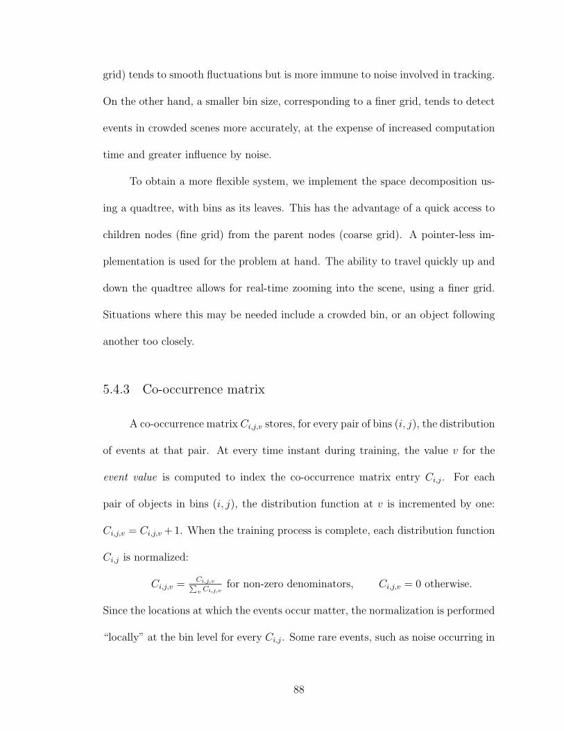
grid) tends to smooth fluctuations but is more immune to noise involved in tracking.
On the other hand, a smaller bin size, corresponding to a finer grid, tends to detect
events in crowded scenes more accurately, at the expense of increased computation
time and greater influence by noise.
To obtain a more flexible system, we implement the space decomposition us-
ing a quadtree, with bins as its leaves. This has the advantage of a quick access to
children nodes (fine grid) from the parent nodes (coarse grid). A pointer-less im-
plementation is used for the problem at hand. The ability to travel quickly up and
down the quadtree allows for real-time zooming into the scene, using a finer grid.
Situations where this may be needed include a crowded bin, or an object following
another too closely.
5.4.3 Co-occurrence matrix
A co-occurrence matrix Ci,j,v stores, for every pair of bins (i, j), the distribution
of events at that pair. At every time instant during training, the value v for the
event value is computed to index the co-occurrence matrix entry Ci,j. For each
pair of objects in bins (i, j), the distribution function at v is incremented by one:
Ci,j,v = Ci,j,v + 1. When the training process is complete, each distribution function
Ci,j is normalized:
Ci,j,v =Ci,j,v∑v Ci,j,v
for non-zero denominators, Ci,j,v = 0 otherwise.
Since the locations at which the events occur matter, the normalization is performed
“locally” at the bin level for every Ci,j. Some rare events, such as noise occurring in
88

a certain bin, might get magnified in this normalization process. A global normal-
ization, where elements of C are normalized by the sum of all its elements might
be considered. Experimental results show that such a matrix normalization is not
sufficiently discriminative.
First order events are naturally reported as unusual with respect to every
other object in the scene. These are further processed to detect the single offending
object. The required training time is decided when the distributions Ci,j tend to
reach a steady state. This is detected by measuring the change in the histograms of
probabilities.
Training is performed at a finest level of the tessellation. Coarse level trained
entries, if needed, are computed by agglomerating the corresponding fine level ones.
Given two large bins x and y at the coarser level, the co-occurrence Cxy is computed
as follows. The sets of children of x and y, Sx and Sy, are computed; then, the
corresponding distributions are added as in the following equation:
Cxy =∑
i,j cij, ∀i ∈ Sx,∀j ∈ Sy,
where c is the co-occurrence matrix at the finer level. The appropriate matrix is
then used to test at the required level.
5.4.4 Detecting unusual events
As mentioned earlier, we define unusual events as non-frequent or rare events.
During the training period, probabilities of first and second order events are com-
puted for every bin or pair of bins, respectively. If, during the test phase, an event
89

is detected as a “low probability event”, it is reported as unusual. Defining low
probability events is quite challenging. A study of the histogram of probabilities is
useful in determining a range of low probabilities. The threshold probability pth,
below which an event is considered unusual, can then be chosen to coincide with a
given cumulative percentage of events.
Diagonal elements of the co-occurrence matrix are used to detect unusual first
order events, i.e. those involving a single object. Once such an event is detected,
its co-occurrences with further objects are ignored.
5.5 Results
5.5.1 Dataset
We built a traffic simulator to generate a “cheap” but rich environment for
agent interactions. We simulate a four-way stop sign, which obeys the rules of traffic
in the US. Figure 5.3 illustrates a typical snapshot of the simulator, with the arrows
indicating driving directions.
The simulator has two built-in sets of rules. The first set generates the usual
behavior that would be expected at a stop sign. It includes different arrival rates
for each lane. According to these rates, vehicles arrive randomly at each lane, flow
towards the stopping line, where they pause until the way is clear. Based on the
order in which they arrived, vehicles are allowed to cross the intersection either
forwards, by making a right turn, or by making a left turn. Usual rules of traffic are
obeyed by not having any two intersecting trajectories.
90
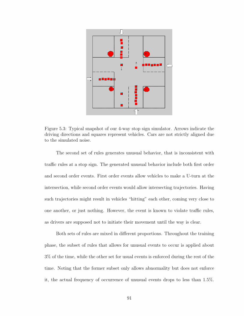
Figure 5.3: Typical snapshot of our 4-way stop sign simulator. Arrows indicate thedriving directions and squares represent vehicles. Cars are not strictly aligned dueto the simulated noise.
The second set of rules generates unusual behavior, that is inconsistent with
traffic rules at a stop sign. The generated unusual behavior include both first order
and second order events. First order events allow vehicles to make a U-turn at the
intersection, while second order events would allow intersecting trajectories. Having
such trajectories might result in vehicles “hitting” each other, coming very close to
one another, or just nothing. However, the event is known to violate traffic rules,
as drivers are supposed not to initiate their movement until the way is clear.
Both sets of rules are mixed in different proportions. Throughout the training
phase, the subset of rules that allows for unusual events to occur is applied about
3% of the time, while the other set for usual events is enforced during the rest of the
time. Noting that the former subset only allows abnormality but does not enforce
it, the actual frequency of occurrence of unusual events drops to less than 1.5%.
91
The simulator might simply “elect” not to generate an intersecting path, even when
it has the opportunity to do so. During the testing phase, a larger set of unusual
events is allowed to occur for a longer period of time, for experimental results only.
A real tracking module is often susceptible to noise. The simulator adds ran-
dom noise to the position of vehicles, resulting in less artificial trajectories.
5.5.2 System training
Timing results are based on experiments performed on a Pentium-M machine
with a processor running at 1.8 GHz with 1 GB RAM.
We train our system on two different simulations, one including noise and
one without. Each training session has a duration of about 10 hours. First and
second order unusual events occur with a rate of about 1.5-2% during the training
period. For the purpose of testing, the simulated data contains unusual events for
approximately 30% of the time in average. We generate over 100 short segments to
obtain the shown results. Each segment runs for up to 7 minutes and contains a
balance of usual versus unusual events for the test. Training is performed for two
levels of spatial subdivision: a coarse grid with 16 bins and a fine grid with 64 bins.
Only the co-occurrence matrix for the fine grid tessellation need to be trained since
the matrix for the coarse grid is computed by coalescing the appropriate adjacent
cells in the former one.
At a simulated resolution of 10 frames per second, using a 64-bin grid, the
time required to train the co-occurrence matrix represents less than 20% of the
92
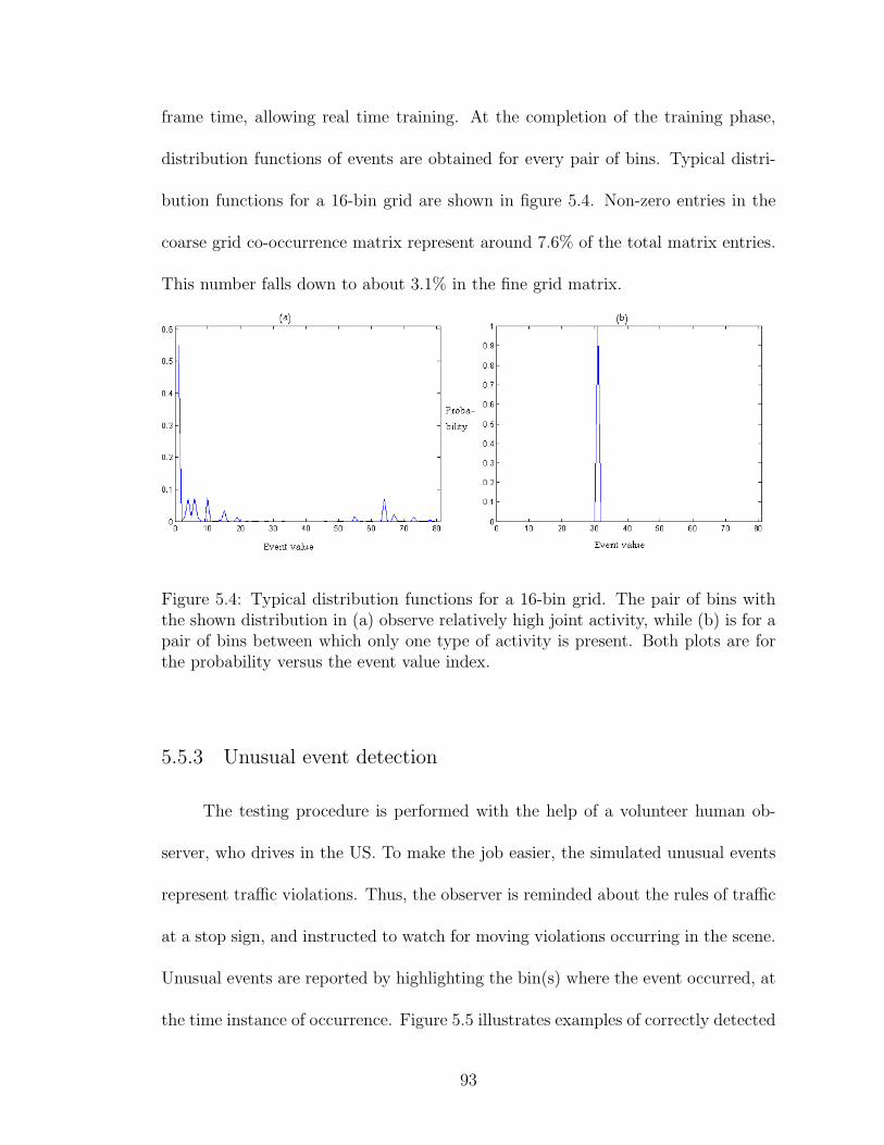
frame time, allowing real time training. At the completion of the training phase,
distribution functions of events are obtained for every pair of bins. Typical distri-
bution functions for a 16-bin grid are shown in figure 5.4. Non-zero entries in the
coarse grid co-occurrence matrix represent around 7.6% of the total matrix entries.
This number falls down to about 3.1% in the fine grid matrix.
Figure 5.4: Typical distribution functions for a 16-bin grid. The pair of bins withthe shown distribution in (a) observe relatively high joint activity, while (b) is for apair of bins between which only one type of activity is present. Both plots are forthe probability versus the event value index.
5.5.3 Unusual event detection
The testing procedure is performed with the help of a volunteer human ob-
server, who drives in the US. To make the job easier, the simulated unusual events
represent traffic violations. Thus, the observer is reminded about the rules of traffic
at a stop sign, and instructed to watch for moving violations occurring in the scene.
Unusual events are reported by highlighting the bin(s) where the event occurred, at
the time instance of occurrence. Figure 5.5 illustrates examples of correctly detected
93
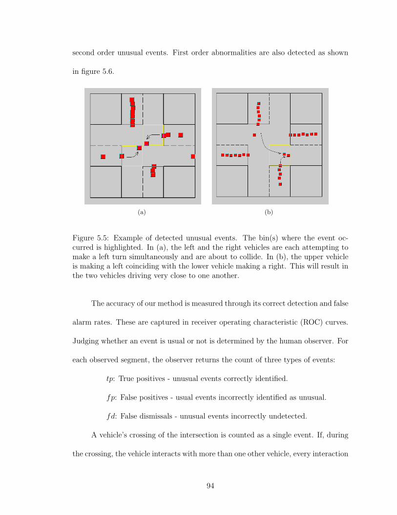
second order unusual events. First order abnormalities are also detected as shown
in figure 5.6.
(a) (b)
Figure 5.5: Example of detected unusual events. The bin(s) where the event oc-curred is highlighted. In (a), the left and the right vehicles are each attempting tomake a left turn simultaneously and are about to collide. In (b), the upper vehicleis making a left coinciding with the lower vehicle making a right. This will result inthe two vehicles driving very close to one another.
The accuracy of our method is measured through its correct detection and false
alarm rates. These are captured in receiver operating characteristic (ROC) curves.
Judging whether an event is usual or not is determined by the human observer. For
each observed segment, the observer returns the count of three types of events:
tp: True positives - unusual events correctly identified.
fp: False positives - usual events incorrectly identified as unusual.
fd: False dismissals - unusual events incorrectly undetected.
A vehicle’s crossing of the intersection is counted as a single event. If, during
the crossing, the vehicle interacts with more than one other vehicle, every interaction
94
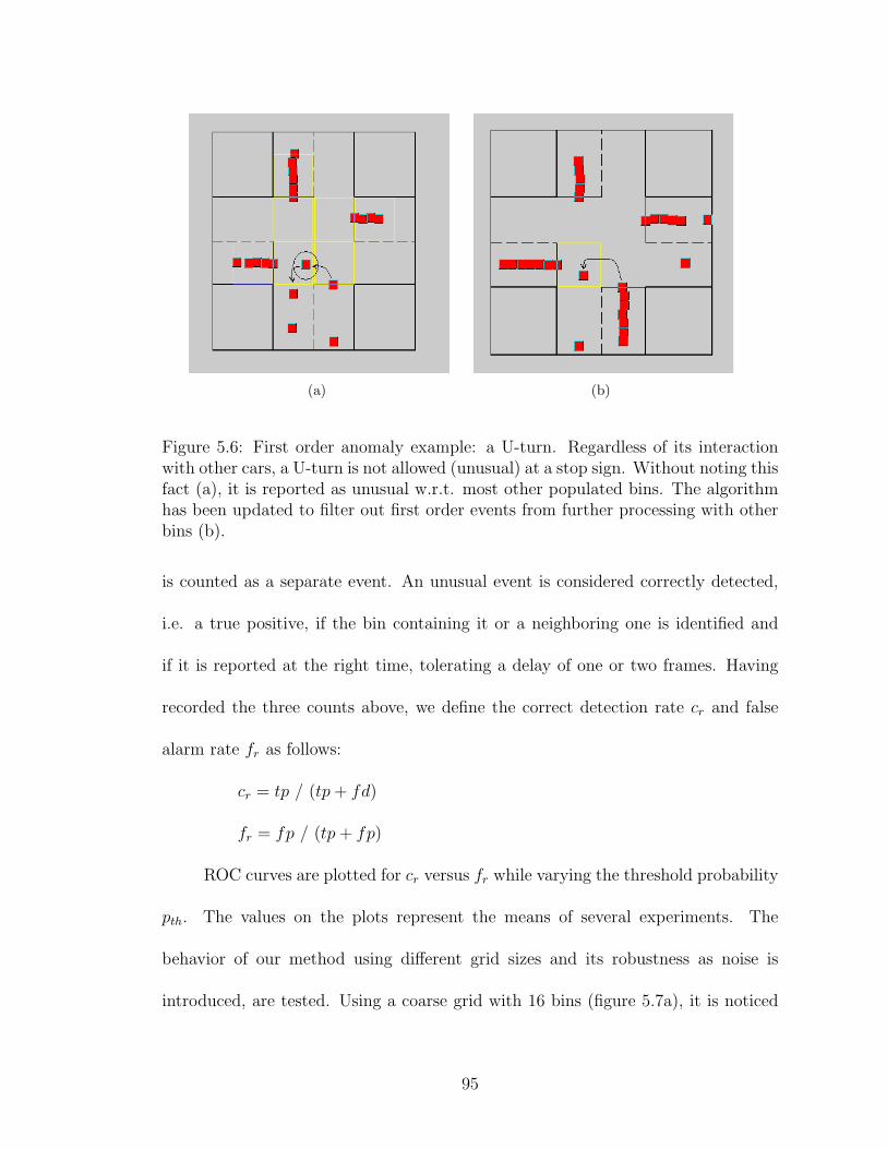
(a) (b)
Figure 5.6: First order anomaly example: a U-turn. Regardless of its interactionwith other cars, a U-turn is not allowed (unusual) at a stop sign. Without noting thisfact (a), it is reported as unusual w.r.t. most other populated bins. The algorithmhas been updated to filter out first order events from further processing with otherbins (b).
is counted as a separate event. An unusual event is considered correctly detected,
i.e. a true positive, if the bin containing it or a neighboring one is identified and
if it is reported at the right time, tolerating a delay of one or two frames. Having
recorded the three counts above, we define the correct detection rate cr and false
alarm rate fr as follows:
cr = tp / (tp + fd)
fr = fp / (tp + fp)
ROC curves are plotted for cr versus fr while varying the threshold probability
pth. The values on the plots represent the means of several experiments. The
behavior of our method using different grid sizes and its robustness as noise is
introduced, are tested. Using a coarse grid with 16 bins (figure 5.7a), it is noticed
95
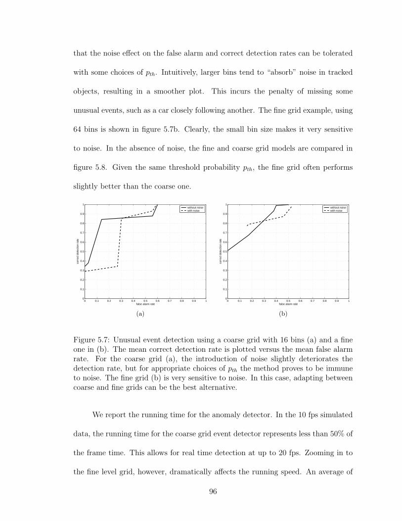
that the noise effect on the false alarm and correct detection rates can be tolerated
with some choices of pth. Intuitively, larger bins tend to “absorb” noise in tracked
objects, resulting in a smoother plot. This incurs the penalty of missing some
unusual events, such as a car closely following another. The fine grid example, using
64 bins is shown in figure 5.7b. Clearly, the small bin size makes it very sensitive
to noise. In the absence of noise, the fine and coarse grid models are compared in
figure 5.8. Given the same threshold probability pth, the fine grid often performs
slightly better than the coarse one.
0 0.1 0.2 0.3 0.4 0.5 0.6 0.7 0.8 0.9 10
0.1
0.2
0.3
0.4
0.5
0.6
0.7
0.8
0.9
1
false alarm rate
corr
ect d
etec
tion
rate
without noisewith noise
(a)
0 0.1 0.2 0.3 0.4 0.5 0.6 0.7 0.8 0.9 10
0.1
0.2
0.3
0.4
0.5
0.6
0.7
0.8
0.9
1
false alarm rate
corr
ect d
etec
tion
rate
without noisewith noise
(b)
Figure 5.7: Unusual event detection using a coarse grid with 16 bins (a) and a fineone in (b). The mean correct detection rate is plotted versus the mean false alarmrate. For the coarse grid (a), the introduction of noise slightly deteriorates thedetection rate, but for appropriate choices of pth the method proves to be immuneto noise. The fine grid (b) is very sensitive to noise. In this case, adapting betweencoarse and fine grids can be the best alternative.
We report the running time for the anomaly detector. In the 10 fps simulated
data, the running time for the coarse grid event detector represents less than 50% of
the frame time. This allows for real time detection at up to 20 fps. Zooming in to
the fine level grid, however, dramatically affects the running speed. An average of
96

0 0.1 0.2 0.3 0.4 0.5 0.6 0.7 0.8 0.9 10
0.1
0.2
0.3
0.4
0.5
0.6
0.7
0.8
0.9
1
false alarm rateco
rrec
t det
ectio
n ra
te
coarse gridfine grid
Figure 5.8: Unusual event detection: coarse and fine grids compared in the absenceof noise. Slightly better performance using the fine grid for many values of pth.
only 1.4 fps can be analyzed. This detection rate can be improved by implementing
techniques for sparse matrices.
We conclude this section by noting that to achieve significantly better perfor-
mance using this model, the coarse grid should be used most of the time, zooming
in to the finer grid only when needed.
5.6 Proposed Extensions
We present in this section several areas that can be improved, and how they
can be addressed. We also propose how the current work can be used for the video
scoring problem. But we start first by showing some limitations of our method when
dealing with real video as opposed to the simulated data used for our results.
97
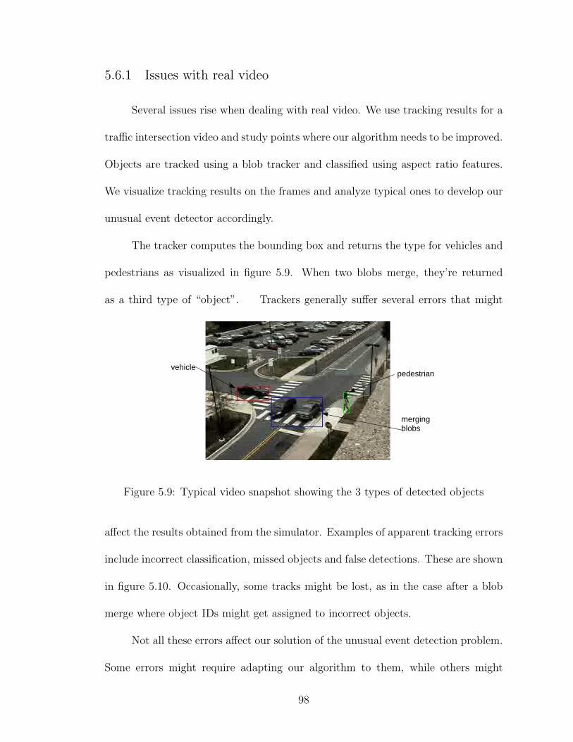
5.6.1 Issues with real video
Several issues rise when dealing with real video. We use tracking results for a
traffic intersection video and study points where our algorithm needs to be improved.
Objects are tracked using a blob tracker and classified using aspect ratio features.
We visualize tracking results on the frames and analyze typical ones to develop our
unusual event detector accordingly.
The tracker computes the bounding box and returns the type for vehicles and
pedestrians as visualized in figure 5.9. When two blobs merge, they’re returned
as a third type of “object”. Trackers generally suffer several errors that might
pedestrian
mergingblobs
vehicle
Figure 5.9: Typical video snapshot showing the 3 types of detected objects
affect the results obtained from the simulator. Examples of apparent tracking errors
include incorrect classification, missed objects and false detections. These are shown
in figure 5.10. Occasionally, some tracks might be lost, as in the case after a blob
merge where object IDs might get assigned to incorrect objects.
Not all these errors affect our solution of the unusual event detection problem.
Some errors might require adapting our algorithm to them, while others might
98
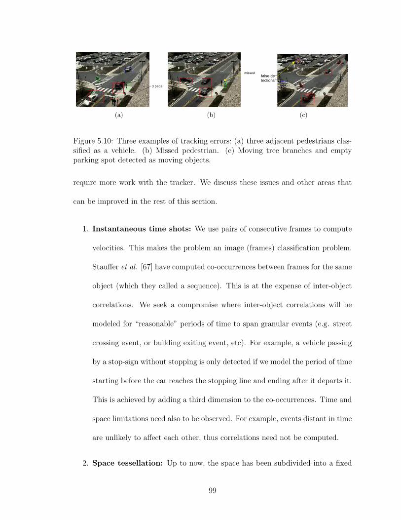
3 peds
(a)
missed
(b)
false de−tections
(c)
Figure 5.10: Three examples of tracking errors: (a) three adjacent pedestrians clas-sified as a vehicle. (b) Missed pedestrian. (c) Moving tree branches and emptyparking spot detected as moving objects.
require more work with the tracker. We discuss these issues and other areas that
can be improved in the rest of this section.
1. Instantaneous time shots: We use pairs of consecutive frames to compute
velocities. This makes the problem an image (frames) classification problem.
Stauffer et al. [67] have computed co-occurrences between frames for the same
object (which they called a sequence). This is at the expense of inter-object
correlations. We seek a compromise where inter-object correlations will be
modeled for “reasonable” periods of time to span granular events (e.g. street
crossing event, or building exiting event, etc). For example, a vehicle passing
by a stop-sign without stopping is only detected if we model the period of time
starting before the car reaches the stopping line and ending after it departs it.
This is achieved by adding a third dimension to the co-occurrences. Time and
space limitations need also to be observed. For example, events distant in time
are unlikely to affect each other, thus correlations need not be computed.
2. Space tessellation: Up to now, the space has been subdivided into a fixed
99

grid for the whole scene. We have used more than one bin size, but that size
has been fixed for the whole scene. Some bins are crowded while others are
almost empty. Results are affected by the displacement of the grid on the
ground.
We suggest several improvements here. Computing co-occurrences need only
be performed between “neighboring” bins. Computing the neighborhood size
is a problem itself. There might be a situation where two nearby locations
don’t interact at all (e.g. separated by a wall). A natural extension of the
fixed grid for real video is a “perspective grid” in the image plane. We need
results to be invariant with respect to the model chosen. A challenging prob-
lem is that of automatically computing an adaptive space tessellation. The
position of the grid will be determined based on trajectories clusters and the
size of bins (variable), based on traffic density.
We also recall that in our results, only about 7.6% of the upper triangular
co-occurrence matrix was non-zero. This is typical of this approach, as in the
results in [39]. Storing using sparse matrix techniques, and avoiding compu-
tations involving zero elements save considerable space and time. Non-zero
elements represent mutual activity. In other words, avoiding zero elements
means that we skip regions without activity.
3. Tracking errors: The simulator has assumed a perfect tracker except for the
generated random noise added to the vehicles locations. This assumption is far
from realistic. To deal with this problem, there are three possible approaches
100

(or a combination thereof).
• Manually correct tracking errors. This approach has been used in [33] and
[35] for example. This approach has the benefit of focusing all effort on
the abnormality detection work, hoping that one day, tracking methods
will be developed enough.
• Enhance the tracker in aspects that benefit the abnormality detector.
One example can be that of learning locations of human and vehicle
trajectories, thus easily considering a car driving up the wall of a building
as a tracker error rather than an unusual event. (We assume of course
that cars cannot drive in general up walls).
• Adjust the abnormality detector to the errors of the tracker. This means
that we admit that any tracker will always have errors that can’t be
fixed in the foreseeable future. An example of this can be to ignore short
“disappearances” of moving objects.
4. Optical flow: Tracking “ensemble” movements or flows rather than individ-
uals tracking is more appealing for crowded scenes and traffic monitoring. We
are more interested in detecting anomalies rather than in tracking individuals.
This approach will involve estimating the distribution of flows in different re-
gions of the surveyed scene, and reporting events that do not fit the estimated
model as unusual.
5. Video scoring: Video segments with unusual activity receive high scores for
101

further manual analysis. Several issues need to be addressed here:
• Splitting the video into segments to be scored
• Choosing a suitable cost function to assign appropriate scores based on
how much the analyzed segment varies from the model estimated for the
video.
102
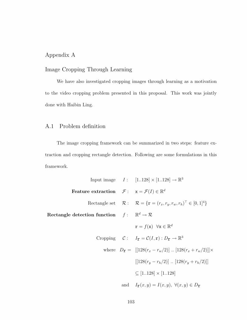
Appendix A
Image Cropping Through Learning
We have also investigated cropping images through learning as a motivation
to the video cropping problem presented in this proposal. This work was jointly
done with Haibin Ling.
A.1 Problem definition
The image cropping framework can be summarized in two steps: feature ex-
traction and cropping rectangle detection. Following are some formulations in this
framework.
Input image I : [1..128]× [1..128] → R3
Feature extraction F : x = F(I) ∈ Rd
Rectangle set R : R = {r = (rx, ry, rw, rh)> ∈ [0, 1]4}
Rectangle detection function f : Rd →R
r = f(x) ∀x ∈ Rd
Cropping C : Ir = C(I, r) : Dr → R3
where Dr = [[128(rx − rw/2)] .. [128(rx + rw/2)]]×
[[128(ry − rh/2)] .. [128(ry + rh/2)]]
⊆ [1..128]× [1..128]
and Ir(x, y) = I(x, y), ∀(x, y) ∈ Dr
103
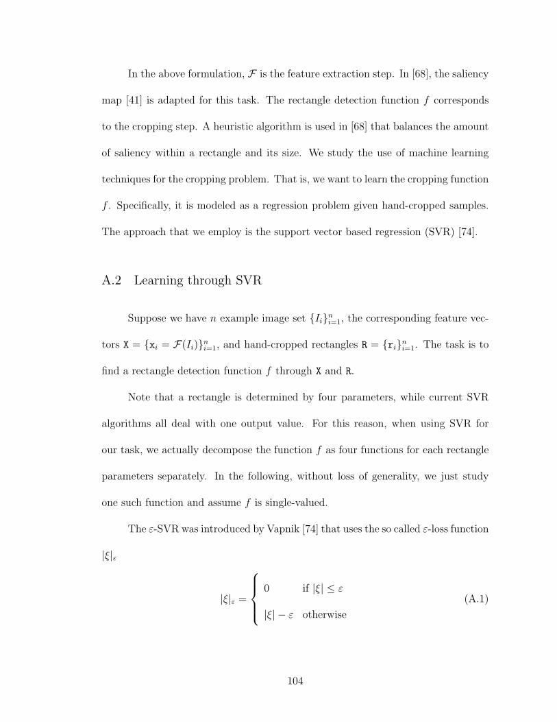
In the above formulation, F is the feature extraction step. In [68], the saliency
map [41] is adapted for this task. The rectangle detection function f corresponds
to the cropping step. A heuristic algorithm is used in [68] that balances the amount
of saliency within a rectangle and its size. We study the use of machine learning
techniques for the cropping problem. That is, we want to learn the cropping function
f . Specifically, it is modeled as a regression problem given hand-cropped samples.
The approach that we employ is the support vector based regression (SVR) [74].
A.2 Learning through SVR
Suppose we have n example image set {Ii}ni=1, the corresponding feature vec-
tors X = {xi = F(Ii)}ni=1, and hand-cropped rectangles R = {ri}n
i=1. The task is to
find a rectangle detection function f through X and R.
Note that a rectangle is determined by four parameters, while current SVR
algorithms all deal with one output value. For this reason, when using SVR for
our task, we actually decompose the function f as four functions for each rectangle
parameters separately. In the following, without loss of generality, we just study
one such function and assume f is single-valued.
The ε-SVR was introduced by Vapnik [74] that uses the so called ε-loss function
|ξ|ε
|ξ|ε =
0 if |ξ| ≤ ε
|ξ| − ε otherwise
(A.1)
104
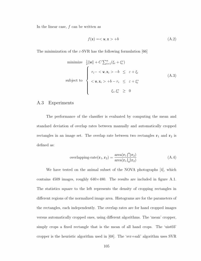
In the linear case, f can be written as
f(x) =< w, x > +b (A.2)
The minimization of the ε-SVR has the following formulation [66]
minimize 12‖w‖+ C
∑ni=1(ξi + ξ∗i )
subject to
ri− < w, xi > −b ≤ ε + ξi
< w, xi > +b− ri ≤ ε + ξ∗i
ξi, ξ∗i ≥ 0
(A.3)
A.3 Experiments
The performance of the classifier is evaluated by computing the mean and
standard deviation of overlap rates between manually and automatically cropped
rectangles in an image set. The overlap rate between two rectangles r1 and r2 is
defined as:
overlapping-rate(r1, r2) =area(r1
⋂r2)
area(r1
⋃r2)
(A.4)
We have tested on the animal subset of the NOVA photographs [4], which
contains 4509 images, roughly 640×480. The results are included in figure A.1.
The statistics square to the left represents the density of cropping rectangles in
different regions of the normalized image area. Histograms are for the parameters of
the rectangles, each independently. The overlap rates are for hand cropped images
versus automatically cropped ones, using different algorithms. The ‘mean’ cropper,
simply crops a fixed rectangle that is the mean of all hand crops. The ‘uist03’
cropper is the heuristic algorithm used in [68]. The ‘svr+sali’ algorithm uses SVR
105
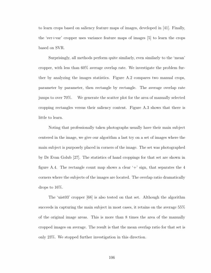
to learn crops based on saliency feature maps of images, developed in [41]. Finally,
the ‘svr+var’ cropper uses variance feature maps of images [5] to learn the crops
based on SVR.
Surprisingly, all methods perform quite similarly, even similarly to the ‘mean’
cropper, with less than 60% average overlap rate. We investigate the problem fur-
ther by analyzing the images statistics. Figure A.2 compares two manual crops,
parameter by parameter, then rectangle by rectangle. The average overlap rate
jumps to over 70%. We generate the scatter plot for the area of manually selected
cropping rectangles versus their saliency content. Figure A.3 shows that there is
little to learn.
Noting that professionally taken photographs usually have their main subject
centered in the image, we give our algorithm a last try on a set of images where the
main subject is purposely placed in corners of the image. The set was photographed
by Dr Evan Golub [27]. The statistics of hand croppings for that set are shown in
figure A.4. The rectangle count map shows a clear ‘+’ sign, that separates the 4
corners where the subjects of the images are located. The overlap ratio dramatically
drops to 16%.
The ‘uist03’ cropper [68] is also tested on that set. Although the algorithm
succeeds in capturing the main subject in most cases, it retains on the average 55%
of the original image areas. This is more than 8 times the area of the manually
cropped images on average. The result is that the mean overlap ratio for that set is
only 23%. We stopped further investigation in this direction.
106
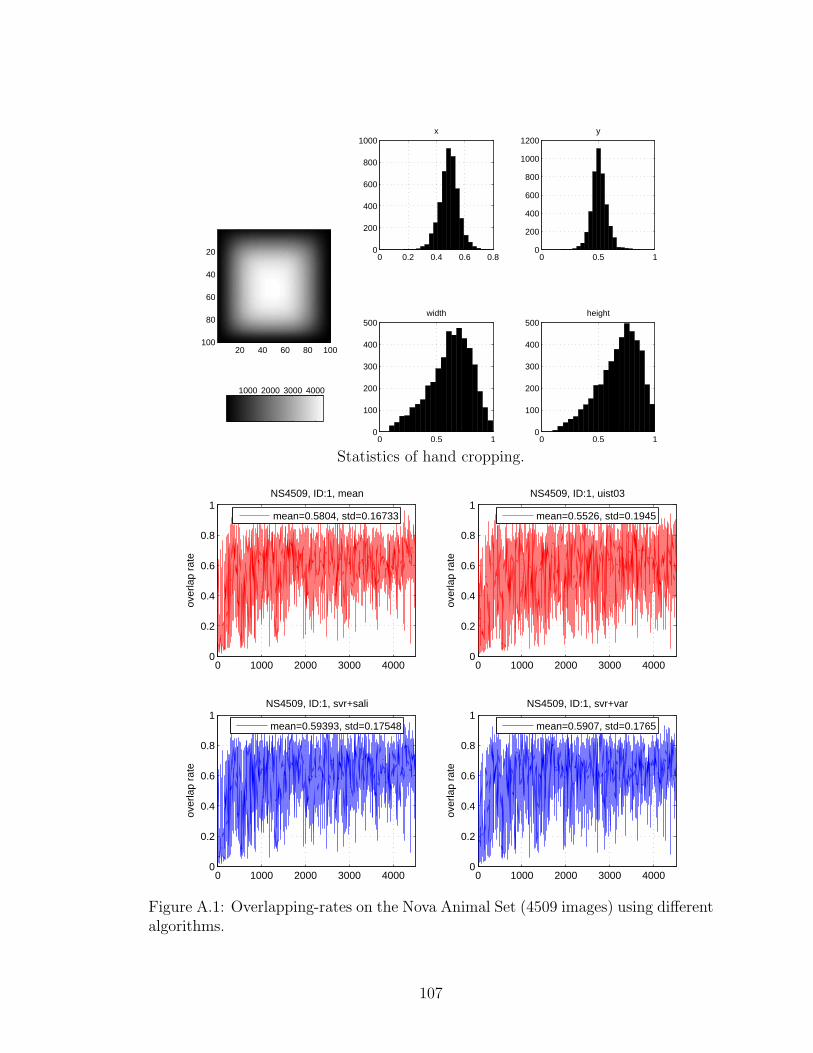
20 40 60 80 100
20
40
60
80
100
1000 2000 3000 4000
0 0.2 0.4 0.6 0.80
200
400
600
800
1000x
0 0.5 10
200
400
600
800
1000
1200y
0 0.5 10
100
200
300
400
500width
0 0.5 10
100
200
300
400
500height
Statistics of hand cropping.
0 1000 2000 3000 40000
0.2
0.4
0.6
0.8
1
over
lap
rate
NS4509, ID:1, mean
mean=0.5804, std=0.16733
0 1000 2000 3000 40000
0.2
0.4
0.6
0.8
1
over
lap
rate
NS4509, ID:1, uist03
mean=0.5526, std=0.1945
0 1000 2000 3000 40000
0.2
0.4
0.6
0.8
1
over
lap
rate
NS4509, ID:1, svr+sali
mean=0.59393, std=0.17548
0 1000 2000 3000 40000
0.2
0.4
0.6
0.8
1
over
lap
rate
NS4509, ID:1, svr+var
mean=0.5907, std=0.1765
Figure A.1: Overlapping-rates on the Nova Animal Set (4509 images) using differentalgorithms.
107
0 2000 40000
0.5
1x Haibin
Hazem
0 2000 4000−0.5
0
0.5mean=0.039742, std=0.049725
diff
0 2000 40000
0.5
1y Haibin
Hazem
0 2000 4000−0.5
0
0.5mean=0.037734, std=0.042567
diff
0 2000 40000
0.5
1width Haibin
Hazem
0 2000 4000−0.5
0
0.5mean=0.091134, std=0.094706
diff
0 2000 40000
0.5
1height Haibin
Hazem
0 2000 4000−0.5
0
0.5mean=0.081893, std=0.081729
diff
0 500 1000 1500 2000 2500 3000 3500 4000 45000
0.5
1overlap rate = intersect area / union area
Haibin’s vs. Hazem’s cropping, mean=0.71654, std=0.19194
Figure A.2: Overlapping-rates on the Nova Animal Set of two manual croppings.
0 0.2 0.4 0.6 0.8 10
0.2
0.4
0.6
0.8
1
Scatter plot of feature fraction vs. area fraction − Hazem
area fraction of cropping rectangle
feat
ure
frac
tion
0 0.2 0.4 0.6 0.8 10
0.2
0.4
0.6
0.8
1
Scatter plot of feature fraction vs. area fraction − Haibin
area fraction of cropping rectangle
feat
ure
frac
tion
S A L I E N C Y M A P
Figure A.3: Scatter plot of rectangle area versus saliency content.
108
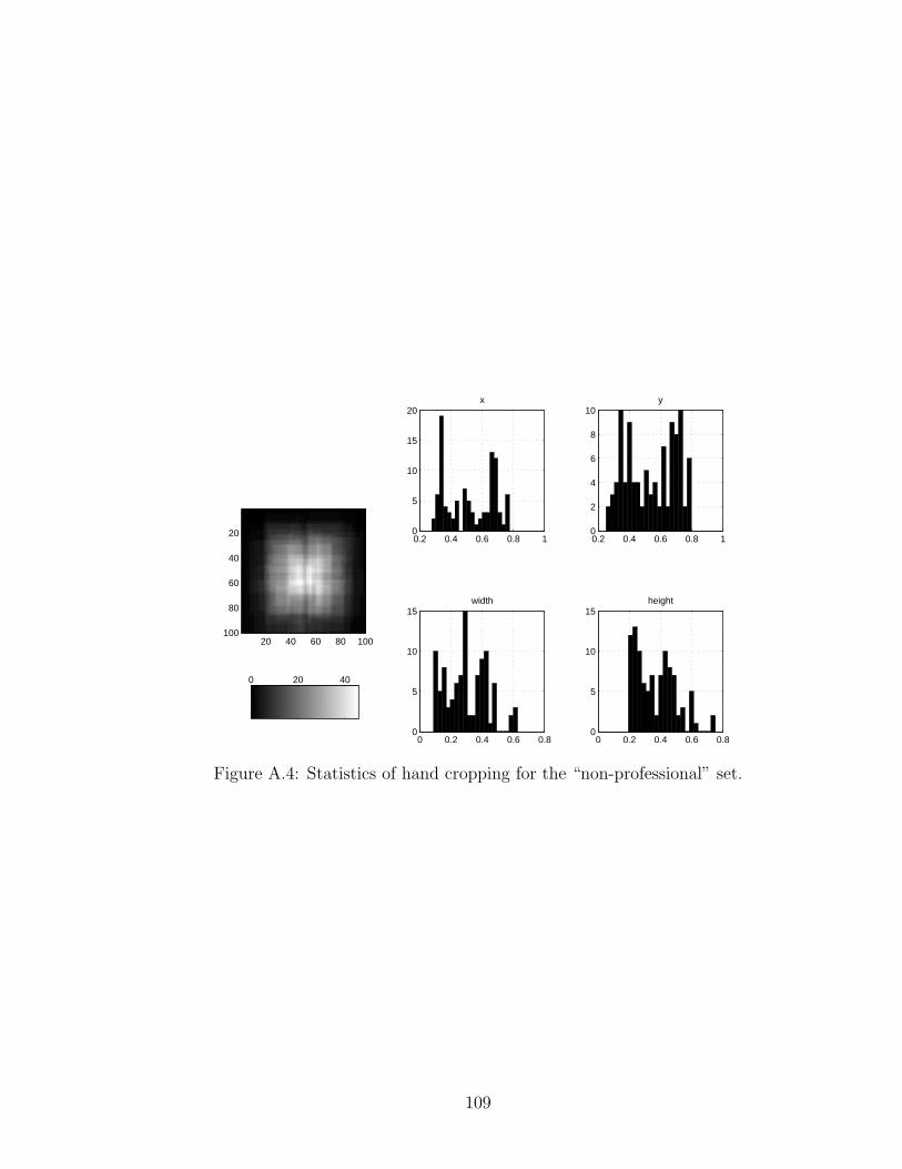
20 40 60 80 100
20
40
60
80
100
0 20 40
0.2 0.4 0.6 0.8 10
5
10
15
20x
0.2 0.4 0.6 0.8 10
2
4
6
8
10y
0 0.2 0.4 0.6 0.80
5
10
15width
0 0.2 0.4 0.6 0.80
5
10
15height
Figure A.4: Statistics of hand cropping for the “non-professional” set.
109
Bibliography
[1] Telindus Surveillance Solutions Ltd, 2005.http://www.telindussurveillance-us.com/.
[2] New York Civil Liberties Union Special Report. Fall 2006.
[3] Cable News Network, CNN 2007. http://www.cnn.com.
[4] Nova development corporation, “Art explosion 300,000”. http://www.novadevelopment.com/Products/us/ahw/default.aspx.
[5] Gaurav Agarwal. Presenting visual information to the user: Combining com-puter vision and interface design. M.S. Thesis, University of Maryland, 2005.
[6] Pankaj K. Agarwal and Cecilia Magdalena Procopiuc. Exact and approximationalgorithms for clustering. Algorithmica, 33(2):201–226, December 2002.
[7] Ravindra K. Ahuja, Kurt Mehlhorn, James Orlin, and Robert E. Tarjan. Fasteralgorithms for the shortest path problem. J. ACM, 37(2):213–223, 1990.
[8] Tirthankar Bandyopadhyay, Marcelo H. Ang Jr, and David Hsu. Motion plan-ning for 3-d target tracking among obstacles. In Proc. International Symposiumon Robotics Research (ISRR’07), Hiroshima, Japan, 2007.
[9] Tirthankar Bandyopadhyay, Yuanping Li, Marcelo H. Ang Jr, and David Hsu.A greedy strategy for tracking a locally predictable target among obstacles. InProc. IEEE International Conference on Robotics and Automation (ICRA’06),pages 2342–2347, Orlando, Florida, May 2006.
[10] Sourabh Bhattacharya, Salvatore Candido, and Seth Hutchinson. Motionstrategies for surveillance. In Proceedings of Robotics: Science and SystemsIII, 2007.
[11] Sourabh Bhattacharya and Seth Hutchinson. Approximation schemes for two-player pursuit evasion games with visibility constraints. In Proceedings ofRobotics: Science and Systems IV, Zurich, Switzerland, June 2008.
[12] Li-Qun Chen, Xing Xie, Xin Fan, Wei-Ying Ma, Hong-Jiang Zhang, and He-Qin Zhou. A visual attention model for adapting images on small displays.Multimedia Systems, 9(4):353–364, Oct 2003.
[13] Robert T. Collins, Alan J. Lipton, Hironobu Fujiyoshi, and Takeo Kanade.Algorithms for cooperative multisensor surveillance. Proceedings of the IEEE,89(10):1456–1477, October 2001.
110
[14] Franklin C. Crow. Summed-area tables for texture mapping. In Proceedingsof the 11th annual conference on Computer graphics and interactive techniques(SIGGRAPH’84), volume 18, pages 207–212, 1984.
[15] Thomas Deselaers, Philippe Dreuw, and Hermann Ney. Pan, zoom, scan −time-coherent, trained automatic video cropping. In IEEE Conference on Com-puter Vision and Pattern Recognition, (CVPR’08), pages 1–8, June 2008.
[16] Robert B. Dial. Algorithm 360: Shortest-path forest with topological ordering[H]. Commun. ACM, 12(11):632–633, 1969.
[17] Edsger W. Dijkstra. A note on two problems in connection with graphs. Nu-merische Mathematik, 1:269–271, 1959.
[18] Dieter Fox Donald J. Patterson, Lin Liao and Henry Kautz. Inferring high-level behavior from low-level sensors. Proc. Fifth International Conference onUbiquitous Computing (UBICOMP ’03), pages 73–89, Oct. 2003.
[19] Thi V. Duong, Hung H. Bui, Dinh Q. Phung, and Svetha Venkatesh. Activityrecognition and abnormality detection with the switching hidden semi-markovmodel. IEEE Computer Society Conference on Computer Vision and PatternRecognition (CVPR ’05), 1:838– 845, June 2005.
[20] Jack Edmonds. Paths, trees, and flowers. Canadian Journal of Mathematics,17:449–467, 1965.
[21] Hazem El-Alfy, David Jacobs, and Larry Davis. Multi-scale video cropping. InProceedings of the 15th international conference on Multimedia (ACM MM’07),pages 97–106, Sep 2007.
[22] Hazem El-Alfy, David Jacobs, and Larry Davis. Assigning cameras to sub-jects in video surveillance systems. In Proc. IEEE International Conference onRobotics and Automation (ICRA’09), pages 837–843, Kobe, Japan, May 2009.
[23] Erhan Baki Ermis, Venkatesh Saligrama, Pierre-Marc Jodoin, and Janusz Kon-rad. Motion segmentation and abnormal behavior detection via behavior clus-tering. In IEEE International Conference on Image Processing, (ICIP’08).,pages 769–772, Oct. 2008.
[24] Xin Fan, Xing Xie, He-Qin Zhou, and Wei-Ying Ma. Looking into video frameson small displays. In ACM international conference on Multimedia (MM’03),pages 247–250, 2003.
[25] Loren Fiore, Guruprasad Somasundaram, Andrew Drenner, and NikolaosPapanikolopoulos. Optimal camera placement with adaptation to dynamicscenes. In Proc. IEEE International Conference on Robotics and Automation(ICRA’08), pages 956–961, Pasadena, California, May 2008.
111
[26] Andreas Girgensohn, John Adcock, Matthew Cooper, Jonathan Foote, andLynn Wilcox. Simplifying the management of large photo collections. InHuman-Computer Interaction (INTERACT’03), pages 196–203, 2003.
[27] Evan Golub. Photocropr: A first step towards computer-supported automaticgeneration of photographically interesting cropping suggestions. Technical Re-port HCIL-2007-12, Univ of Maryland, Maryland, USA, 2007.
[28] Teofilo F. Gonzalez. Covering a set of points in multidimensional space. Infor-mation Processing Letters, 40(4):181–188, November 1991.
[29] Hector H. Gonzalez-Banos, Cheng-Yu Lee, and Jean-Claude Latombe. Real-time combinatorial tracking of a target moving unpredictably among obsta-cles. In Proc. IEEE International Conference on Robotics and Automation(ICRA’02), pages 1683–1690, Washington, DC, USA, May 2002.
[30] Amit Goradia, Zhiwei Cen, Clayton Haffner, Ning Xi, and Matt Mutka.Switched video feedback for sensor deployment and target tracking in a surveil-lance network. In Proc. IEEE International Conference on Robotics and Au-tomation (ICRA’07), pages 3470–3475, Roma, Italy, April 2007.
[31] Raffay Hamid, Amos Johnson, Samir Batta, Aaron Bobick, Charles Isbell, andGraham Coleman. Detection and explanation of anomalous activities: Repre-senting activities as bags of event n-grams. IEEE Computer Society Conferenceon Computer Vision and Pattern Recognition (CVPR ’05), 1:1031–1038, June2005.
[32] Rachel Heck, Michael Wallick, and Michael Gleicher. Virtual videography.ACM Transactions on Multimedia Computing, Communications and Applica-tions (TOMCCAP), 3(1):4, Feb 2007.
[33] David C. Hogg and Hannah M. Dee. Detecting inexplicable behavior. Proc.British Machine Vision Conference (BMVC ’04), Sept. 2004.
[34] David C. Hogg and Hannah M. Dee. On the feasibility of using a cognitivemodel to filter surveillance data. IEEE Conference on Advanced Video andSignal Based Surveillance (AVSS ’05), pages 34–39, Sept. 2005.
[35] David C. Hogg and Hannah M. Dee. Navigational strategies and surveillance.Sixth IEEE International Workshop on Visual Surveillance (ECCV-VS ’06),May 2006.
[36] David Hsu, Wee Sun Lee, and Nan Rong. A point-based POMDP plannerfor target tracking. In Proc. IEEE International Conference on Robotics andAutomation (ICRA’08), pages 2644–2650, Pasadena, California, May 2008.
[37] Weiming Hu, Xuejuan Xiao, Zhouyu Fu, Dan Xie, Tieniu Tan, and Steve May-bank. A system for learning statistical motion patterns. IEEE Transactions on
112
Pattern Analysis and Machine Intelligence (TPAMI), 28(9):1450–1464, Sept.2006.
[38] Hayley Hung and Shaogang Gong. Quantifying temporal saliency. BritishMachine Vision Conference (BMVC’04), pages 727–736, Sept. 2004.
[39] Hayley Hung and Shaogang Gong. Detecting and quantifying unusual interac-tions by correlating salient motion. IEEE Conference on Advanced Video andSignal Based Surveillance (AVSS ’05), pages 46–51, Sept. 2005.
[40] Laurent Itti and Pierre Baldi. A principled approach to detecting surprisingevents in video. IEEE Computer Society Conference on Computer Vision andPattern Recognition (CVPR’05), 1:631–637, June 2005.
[41] Laurent Itti, Christof Koch, and Ernst Niebur. A model of saliency-based visualattention for rapid scene analysis. IEEE Transactions on Pattern Analysis andMachine Intelligence (TPAMI), 20(11):1254–1259, Nov. 1998.
[42] Timor Kadir and Michael Brady. Saliency, scale and image description. Inter-national Journal of Computer Vision (IJCV), 45(2):83–105, Nov. 2001.
[43] Hong-Wen Kang, Xue-Quan Chen, Yasuyuki Matsushita, and Xiaoou Tang.Space-time video montage. IEEE Computer Society Conference on ComputerVision and Pattern Recognition (CVPR’06), 2:1331–1338, June 2006.
[44] Stephen Kloder and Seth Hutchinson. Partial barrier coverage: Using gametheory to optimize probability of undetected intrusion in polygonal environ-ments. In Proc. IEEE International Conference on Robotics and Automation(ICRA’08), pages 2671–2676, Pasadena, California, May 2008.
[45] Andreas Kolling and Stefano Carpin. The graph-clear problem: definition,theoretical properties and its connections to multirobot aided surveillance. InProc. IEEE/RSJ International Conference on Intelligent Robots and Systems(IROS’07), pages 1003–1008, San Diego, California, 2007.
[46] Andreas Kolling and Stefano Carpin. Extracting surveillance graphs from robotmaps. In Proc. IEEE/RSJ International Conference on Intelligent Robots andSystems (IROS’08), pages 2323–2328, Nice, France, 2008.
[47] Andreas Kolling and Stefano Carpin. Multi-robot surveillance: an improvedalgorithm for the GRAPH-CLEAR problem. In Proc. IEEE International Con-ference on Robotics and Automation (ICRA’08), pages 2360–2365, Pasadena,California, May 2008.
[48] Andreas Kolling and Stefano Carpin. Probabilistic graph clear. In Proc.IEEE/RSJ International Conference on Robotics and Automation (ICRA’09),pages 3508–3514, Kobe, Japan, May 2009.
113
[49] Harold W. Kuhn. The Hungarian method for the assignment problem. NavalResearch Logistics Quarterly, 2:83–97, 1955.
[50] Steven M. LaValle. Planning Algorithms. Cambridge University Press, NewYork, NY, USA, 2006.
[51] Lin Liao, Dieter Fox, and Henry Kautz. Learning and inferring transportationroutines. Proc. National Conference on Artificial Intelligence (AAAI ’04), 2004.
[52] Feng Liu and Michael Gleicher. Video retargeting: automating pan and scan. InACM international conference on Multimedia (MM’06), pages 241–250, 2006.
[53] Dimitrios Makris, Tim Ellis, and James Black. Bridging the gaps betweencameras. In Proc. IEEE Computer Society Conference on Computer Visionand Pattern Recognition (CVPR’04), pages 205–210, Washington, DC, 2004.
[54] Dimitrios Makris and Tim J. Ellis. Spatial and probabilistic modelling of pedes-trian behaviour. British Machine Vision Conference (BMVC ’02), pages 557–566, Sept. 2002.
[55] Dimitri Marinakis, Gregory Dudek, and David J. Fleet. Learning sensor net-work topology through monte carlo expectation maximization. In Proc. IEEEInternational Conference on Robotics and Automation (ICRA’05), pages 4581–4587, Barcelona, Spain, April 2005.
[56] Christian Micheloni, Lauro Snidaro, and GianLuca Foresti. Statistical eventanalysis for video surveillance. Sixth IEEE International Workshop on VisualSurveillance (ECCV-VS ’06), May 2006.
[57] Vlad I. Morariu, V. Shiv Naga Prasad, and Larry S. Davis. Human activityunderstanding using visibility context. In IEEE/RSJ IROS Workshop: Fromsensors to human spatial concepts (FS2HSC ’07), Oct. 2007.
[58] R. Morris and D. Hogg. Statistical models of object interaction. InternationalJournal of Computer Vision (IJCV), 37(2):209–215, June 2000.
[59] Rafael Murrieta-Cid, Raul Monroy, Seth Hutchinson, and Jean-Paul Laumond.A complexity result for the pursuit-evasion game of maintaining visibility ofa moving evader. In Proc. IEEE International Conference on Robotics andAutomation (ICRA’08), pages 2657–2664, Pasadena, California, May 2008.
[60] Rafael Murrieta-Cid, Teja Muppirala, Alejandro Sarmiento, Sourabh Bhat-tacharya, and Seth Hutchinson. Surveillance strategies for a pursuer with finitesensor range. The International Journal of Robotics Research, 26(3):233–253,March 2007.
[61] Joseph O’Rourke. Art Gallery Theorems and Algorithms. Oxford UniversityPress, New York, 1987.
114
[62] Christos H. Papadimitriou and Kenneth Steiglitz. Combinatorial Optimization:Algorithms and Complexity. Prentice Hall, Englewood Cliffs, N.J., 1982.
[63] Fatih Porikli and Ajay Divakaran. Multi-camera calibration, object trackingand query generation. In Proc. International Conference on Multimedia andExpo (ICME’03), pages 653–656, Baltimore, MD, USA, July 2003.
[64] Yong Rui, Liwei He, Anoop Gupta, and Qiong Liu. Building an intelligent cam-era management system. In Proceedings of the Ninth ACM International Con-ference on Multimedia (ACM MM’01), pages 2–11, Ottawa, Canada, September2001.
[65] Justus Schwartz, Angelika Steger, and Andreas Weißl. Covering a set of pointsin multidimensional space. Experimental and Efficient Algorithms, 3503:476–487, May 2005.
[66] Alex J Smola and Bernhard Scholkopf. A tutorial on support vector regression.Statistics and Computing, 14:199–222, Aug. 2004.
[67] Chris Stauffer and W. Eric L. Grimson. Learning patterns of activity usingreal-time tracking. IEEE Transactions on Pattern Analysis and Machine In-telligence (TPAMI), 22(8):747–757, Aug. 2000.
[68] Bongwon Suh, Haibin Ling, Benjamin B. Bederson, and David W. Jacobs.Automatic thumbnail cropping and its effectiveness. ACM Symposium on UserInterface Software and Technology (UIST’03), pages 95–104, Nov. 2003.
[69] Noriko Takemura and Jun Miura. View planning of multiple active camerasfor wide area surveillance. In Proc. IEEE International Conference on Roboticsand Automation (ICRA’07), pages 3173–3179, Roma, Italy, April 2007.
[70] Pang-Ning Tan, Michael Steinbach, and Vipin Kumar. Introduction to DataMining. Pearson, Addison Wesley, 2006.
[71] Zhijun Tang and Umit Ozguner. Motion planning for multitarget surveillancewith mobile sensor agents. IEEE Transactions on Robotics, 21(5):898–908,October 2005.
[72] Toshiba America Information Systems, Inc. [www.toshibasecurity.com].Toshiba IP Network PTZ Camera data sheet, IK-WB21A, 2007.
[73] Jur van den Berg, Sachin Patil, Jason Sewall, Dinesh Manocha, and MingLin. Interactive navigation of multiple agents in crowded environments. InProceedings of the 2008 symposium on interactive 3D graphics and games (I3D’08), pages 139–147, Redwood City, CA, February 2008.
[74] Vladimir N. Vapnik. The Nature of Statistical Learning Theory. Springer, NewYork, 1995.
115
[75] Namrata Vaswani, Amit Roy Chowdhury, and Rama Chellappa. "ShapeActivity": A continuous-state HMM for moving/deforming shapes with ap-plication to abnormal activity detection. IEEE Trans. on Image Processing,14(10):1603–1616, Oct. 2005.
[76] Marcos A M Vieira, Ramesh Govindan, and Gaurav S. Sukhatme. Optimalpolicy in discrete pursuit-evasion games. Technical Report 08-900, Univ ofSouthern California, California, USA, 2008.
[77] Marcos A M Vieira, Ramesh Govindan, and Gaurav S. Sukhatme. Optimalpolicy in discrete pursuit-evasion games. In Proc. International Conference onRobot Communication and Coordination ROBOCOMM ’09, Odense, Denmark,April 2009.
[78] Paul Viola and Michael Jones. Robust real-time face detection. InternationalJournal of Computer Vision, 57(2):137–157, May 2004.
[79] Jun Wang, Marcel J.T. Reinders, Reginald L. Lagendijk, Jasper Lindenberg,and Mohan S. Kankanhalli. Video content representation on tiny devices. IEEEInternational Conference on Multimedia and Expo (ICME’04), 3:1711– 1714,June 2004.
[80] Christopher R. Wren, U. Murat Erdem, and Ali J. Azarbayejani. Automaticpan-tilt-zoom calibration in the presence of hybrid sensor networks. In Pro-ceedings of the Third ACM International Workshop on Video Surveillance &Sensor Networks (VSSN’05), pages 113–120, Singapore, November 2005.
[81] Tao Xiang and Shaogang Gong. Video behaviour profiling and abnormalitydetection without manual labelling. Tenth IEEE International Conference onComputer Vision (ICCV ’05), 2:1238–1245, Oct. 2005.
[82] Tao Xiang and Shaogang Gong. Incremental visual behaviour modelling. SixthIEEE International Workshop on Visual Surveillance (ECCV-VS ’06), May2006.
[83] Xing Xie, Hao Liu, Simon Goumaz, and Wei-Ying Ma. Learning user interestfor image browsing on small-form-factor devices. In SIGCHI Conference onHuman Factors in Computing Systems (CHI’05), pages 671–680, 2005.
[84] Jingjin Yu and Steven M. LaValle. Tracking hidden agents through shadowinformation spaces. In Proc. IEEE International Conference on Robotics andAutomation (ICRA’08), pages 2331–2338, Pasadena, California, May 2008.
[85] Jian Zhao and Sen ching S. Cheung. Multi-camera surveillance with visual tag-ging and generic camera placement. In First ACM/IEEE International Con-ference on Distributed Smart Cameras (ICDSC ’07), pages 259–266, Vienna,Austria, 2007.
116

[86] Hua Zhong, Jianbo Shi, and Mirko Visontai. Detecting unusual activity invideo. IEEE Computer Society Conference on Computer Vision and PatternRecognition (CVPR ’04), 2:819–826, June 2004.
117


![Innovative Mining Techniques and Technologies Review of ...komag.eu/images/maszynygornicze1/MM2020/MiningMachines2-20… · Double drum winder of BB-3000/B type [KOMAG] Double drum](https://img.pdfslide.us/doc/110x75/6095c0de50ddc87a6b521f52/innovative-mining-techniques-and-technologies-review-of-komageuimagesmaszynygornicze1mm2020miningmachines2-20.jpg)


![[Drum] Jim Chapin - Advanced Techniques for the Modern Drummer](https://img.pdfslide.us/doc/110x75/544e67a5b1af9f2f638b4eaf/drum-jim-chapin-advanced-techniques-for-the-modern-drummer.jpg)