– 1 –

Abstract Syntax and Semantics of Visual Languages

Martin ErwigFernUniversität Hagen, Praktische Informatik IV

58084 Hagen, Germanyerwig@fernuni-hagen.de

Abstract

The effective use of visual languages requires a precise understanding of their meaning.Moreover, it is impossible to prove properties of visual languages like soundness of transforma-tion rules or correctness results without having a formal language definition. Although thissounds obvious, it is surprising that only little work has been done about the semantics of visuallanguages, and even worse, there is no general framework available for the semantics specifi-cation of different visual languages. We present such a framework that is based on a rather gen-eral notion of abstract visual syntax. This framework allows a logical as well as a denotationalapproach to visual semantics, and it facilitates the formal reasoning about visual languagesand their properties. We illustrate the concepts of the proposed approach by defining abstractsyntax and semantics for the visual languages VEX, Show and Tell, and Euler Circles. We dem-onstrate the semantics in action by proving a rule for visual reasoning with Euler Circles andby showing the correctness of a Show and Tell program.

1. Introduction

Investigating the semantics of visual languages is important for several reasons: First of all, aprecise definition of semantics is indispensable for a thorough understanding of any language.This in turn is important to appraise a visual language and to compare it to others. Furthermore,this facilitates the development of extensions or a re-design of the language. Second, having aprecise specification of a language’s semantics, it is in many cases only a small step toward animplementation, for instance, denotational semantics can be translated almost verbatim intofunctional languages, so that an interpreter for the language is immediately available [17].Third, with a precise semantics, various properties of languages can be proved. In particular,we can prove syntactic transformations to be sound with respect to the semantics, for example,β-reduction in VEX can be shown to realize function application, or rules for syllogistic rea-soning in Euler diagrams can be proved sound. Finally, a clear semantics of visual languages isneeded to integrate them correctly into other environments. This especially applies to heteroge-neous or multi-paradigm languages, see for example [10].

Despite the reasons just mentioned, research on visual language semantics is rather spo-radic. In particular, there is no general framework available which could be used for the formalspecification of visual languages. This situation is quite different in textual languages: there wecan choose among a variety of different semantic formalisms, such as denotational semantics,structured operational semantics, action semantics, evolving algebras, etc., and some of thesecould, in principle, be employed for visual languages as well. A possible reason why this doesnot happen might be that some of the components that are necessary for a semantics frameworkare missing. Taking denotational semantics as an example, we observe that – at least as far as

– 2 –

visual programming languages are concerned – the necessary concepts of semantic functionand semantic domain can be used as in the textual case. However, the third component,abstract syntax, cannot be simply taken for visual languages, and there is no equivalent notionfor visual languages yet.

So in the sequel we will first introduce a concept of abstract visual syntax in Section 2before we demonstrate the specification of logical and denotational semantics in Sections 3 and4 by two simple examples. In Section 5 we show that also more complex visual languages canbe dealt with by the presented approach. Section 6 comments on related work, and Section 7presents some conclusions.

2. Abstract Visual Syntax

A textual languageL is a set of strings over an alphabetA, that is,L ⊆ A*. The symbols of anysentence (or word) w ∈ L are only related to each other by a linear ordering. In contrast, a sen-tence (or diagram or picture)p of a visual languageVL over an alphabetA consists of a set ofsymbols ofA that are, in general, related by several relationships {r1, …, rn} = R. Thus we cansay that a picturep is given by a pair (s, r) wheres ⊆ A is the set of symbols of the picture andr ⊆ s×R×s gives the relationships that hold inp.1 In other words,p is nothing but a directedgraph with edge labels drawn fromR, and a visual language is simply a set of such graphs.

Usually, languages contain a certain structure, that is, there are precise rules defining whichsymbols can occur in which contexts and, regarding visual languages, which symbols may takepart in which relationships. This structure is recognized and enforced during syntax analysis,and it can be assumed when defining semantics. Therefore, semantics definitions are oftenbased on so-calledabstract syntax which defines a language on a more abstract level with lessconstraints than on the concrete level. This means that a description of concrete syntax mustinclude every detail about the language whereas the abstract syntax can safely ignore allaspects that are not needed within the semantics definition.

A precise definition of abstract syntax does not exist, and it would not make much sensebecause there are different levels of “abstractness” that can be dealt with. One reason forabstract syntax not really having found its way into visual languages might be that, as webelieve, abstract visual syntax must be “more abstract” than in the textual case to be helpful.We explain this by a simple example. Consider the following (textual) grammar describing partof a concrete syntax for expressions.

expr::= n-expr | b-expr | if-exprn-expr::= term | n-expr + termterm::= factor | term * factorfactor::= id | (n-expr)b-expr::= id | b-expr ∨ b-expr | …if-expr::= if b-expr then expr else expr

A corresponding abstract syntax would ignore many details, such as the choice of key words,grammar rules for defining associativity of operators, or rules restricting the typing of opera-tions (see also [17]):

expr::= id | expr op expr | if (expr, expr, expr)op ::= + | * |∨ | …

1. Relationships with arity > 2 can always be simulated by several binary relationships.

– 3 –

This grammar is much more concise. It does not introduce nonterminals for expressions of dif-ferent types, and it also ignores associativity of operators. (Omitting the key words from theconditional does not make the grammar essentially simpler in this example.) Further operationson sentences of the language can rely on syntax being already checked by a parser and can thuswork with the simpler abstract syntax.

In a similar way, the abstract syntax of visual languages need not be concerned with all thedetails that a concrete syntax specification has to care about, see also [8]. This means we canabstract from the choice of icons or symbols (comparable to the choice of key words in the tex-tual case) and from geometric details such as size and position of objects (at least up to topo-logical equivalence, that is, as long as relevant relationships between objects are not affected).We can also ignore associativities used to resolve ambiguous situations during parsing muchlike in the textual example. Moreover, typings of relationships that restrict relationships to spe-cific subsets of symbols can be omitted. This corresponds to grouping operations, such as + or∨, under one nonterminal.

But we can do even more – and this is the point where abstract visual syntax gets moreabstract than in the textual case: the above abstract syntax for expressions is still given by agrammar and thus retains some structural information about the language. This is absolutelyadequate since the description is very simple and can be easily used when defining, for exam-ple, an interpreter for expressions. However, to do so for a visual language requires, in mostcases, some effort in the consideration of context information which unnecessarily complicatesdefinitions of transformations. Therefore, we suggest to forget about this structural informa-tion, too, and to consider a picture just as a directed, labeled multi-graph where the nodes rep-resent objects and the edges represent relationships between objects. A class of graphs is thenjust given by two types defining node and edge labels, that is, the types of objects and relation-ships in the abstractly represented visual language.

Definition 1. A directed labeled multi-graph of type (α, β) is a quintupleG = (V, E, ι, ν, ε) con-sisting of a set of nodesV and a set of edgesE whereι : E → V × V is a total mapping definingfor each edge the nodes it connects. The mappingsν : V → α andε : E → β define the nodeand edge labels.

VG andEG denote the set of nodes and edges ofG. The successors of a node are denoted bysuccG(v), which is defined bysuccG(v) = {w ∈ VG | ∃e ∈ EG: ι(e) = (v, w)}. Lik ewise,predG(v)denotesv’s predecessors. WheneverG is clear from the context, we also might simply useV, E,succ, andpred. We also sometimes use a shorthand for denoting nodes and edges together withtheir labels: we denote a node (or edge)x with ν(x) = l (respectively, ε(x) = l) simply byx:l.

The label typesα andβ might be just sets of symbols, or they can be complex structures toenable the labeling with terms, semantic values, or even graphs (see Section 5). The set of allgraphs of type (α, β) is denoted byΓ(α, β). In the sequel we will look at visual languages onthis very abstract level, that is, the abstract syntax of a visual language is specified as a set ofgraphs of a specific type.

Definition 2. A visual language of type (α, β) is a set of graphsVL ⊆ Γ(α, β).

How does this view relate to the well-established grammatical approach to syntax? Clearly, thesyntax of languages can be conveniently specified by grammars. Grammars provide a way togenerate all sentences of the language and, given a suitable parsing algorithm, allow to testwhether a sentence is a member of the language (possibly giving a proof for this by construct-ing a parse tree for reconstructing the sentence). Concerning abstract syntax, however, gram-

– 4 –

mars are usually not used for parsing; their purpose is just to offer an inductive ordecompositional view of language that facilitates semantics definitions, especially, denota-tional semantics or structured operational semantics. As demonstrated in [7] we can actuallyhave a (de)compositional/recursive view of graphs without resorting to grammars. So we canachieve a highly abstract comprehension of pictures together with an inductive view of graphsthat facilitates, say, denotational semantics definitions. On the other hand, there are visual lan-guages whose semantics are best described in a logical fashion. In that case a global, set-theo-retic view of language is needed, which is just given by abstract visual syntax (and which mightbe obscured when using grammatical formalisms).

As in the textual case the choice of abstract syntax for a visual language is by no meansunique. Usually, one has to trade similarity to the original notation for simplicity of the seman-tics definition. We will illustrate this point further in Section 4. The use of abstract syntax is notrestricted to the definition of language semantics, but it can be also used as a basis for transfor-mations between different languages or for mapping between different representations of thesame language. This is illustrated in more detail in [8]. Accidentally, the abstract syntax graphsfor the examples used in this paper are all acyclic. This is by no means essential for the pre-sented formalism. Examples for visual languages that have cyclic abstract syntax graphs arestate diagrams (syntax and semantics for these are defined in [8]) or a particular representationof Turing machines (for which syntax and semantics can be found in [9]).

3. Logical Semantics

In many cases, a logical specification of semantics views the syntactic elements simply as sets.For graphs, the node- and edge-set view is implicit in the definition. In Section 3.1 we definesyntax and semantics of the well-known Euler diagrams, and in Section 3.2 we prove a visualrule for syllogistic reasoning and thus illustrate how to establish properties of a formalizedvisual language.

3.1 Euler Diagrams

The language of Euler diagrams as described in [11, 20] contains four kinds of basic picturesexpressing logical statements:

Ambiguities of Euler diagrams and semantic problems arising from these are discussed indetail in [20]. Our aim is not arguing in favor of or against using Euler diagrams for reasoning.However, as a matter of fact, Euler diagrams are a wide-spread visual notation, and in order todiscuss the notation and compare it with others, it should be understood in the first place. Thisis what abstract visual syntax and the semantic formalism can accomplish.

The concrete syntax of Euler diagrams comprises circles and string-labels together with therelationshipsinside, intersects, anddisjoint. Labels have two purposes: first, they provide refer-ences to set symbols in pictures to be used in explanations, discussions, etc. Second, their posi-tion distinguishes two different set relationships for intersecting circles. In the abstract syntax

AB

All A is B

A B

No A is B

A B

SomeA is B

Figure 1: Euler Diagrams

A B

SomeA is notB

– 5 –

we can therefore omit labels and replace theintersects-relationship by two edge labels identify-ing the third and fourth situations, namely, p-intersects andnic. The names result from the fol-lowing observations: in order to give a formal semantics to Euler diagrams one has to answerthe following questions (among others):

(1) Does the third situation also say: “SomeB is not A” ? Yes, Euler also specifies that“SomeA is notB” (and “SomeB is A”). Thus we know:

(a) A ∩ B ≠ ∅,(b) A - B ≠ ∅, and(c) B - A ≠ ∅.

So this situation describes what we callproper intersection, that is, we sayA p-intersectsB.

(2) Is the relative position of labels irrelevant, that is, does the last example also say “SomeB is not A” ? This would be reasonable, and although Euler gives as one possibleinstance an example whereB is completely inside (that is, properly included in)A, hehimself uses the notation in a symmetric way later on in his letters. Accordingly, weignore relative positions of labels. So this relationship describes that both differences arenon-empty which expresses nothing but the fact that two sets are not comparable withrespect to inclusion; we call this relationshipnot inclusion-comparable.

Exceptinside, all relationships are symmetric. We depict a symmetric relationship by an undi-rected edge which is represented in a directed graph by two directed edges in both directions.So the abstract syntax graphs for the Euler diagrams of Figure 1 look like:

The semantics is defined for a diagram relative to auniverse of objectsU. An interpretation is amapping from the set of circles in the diagram, that is, nodes of the graph, to subsets ofU, thatis, f : V → 2U. Now the semantics can be easily defined:

S[[ (V, E) ]]U = {f | f : V → 2U ∧ ∀e ∈ E: valid(f, ι(e), ε(e))}

where f(u) ⊆ f(v) if l = inside f(u) ∩ f(v) = ∅ if l = disjoint

valid(f, (u, v), l) = f(u) ∩ f(v) ≠ ∅ ∧ f(u) - f(v) ≠ ∅ ∧ f(v) - f(u) ≠ ∅ if l = p-intersects f(u) - f(v) ≠ ∅ ∧ f(v) - f(u) ≠ ∅ if l = nic

3.2 Soundness of Visual Reasoning Rules

Having a precise definition of what Euler diagrams mean it is quite easy to check the visualrules for syllogistic reasoning. Euler gives textual versions of such rules and explains them bypictures. One example is:

Figure 2: Abstract Syntax Graphs for Euler Diagrams

inside disjoint p-intersects nic

– 6 –

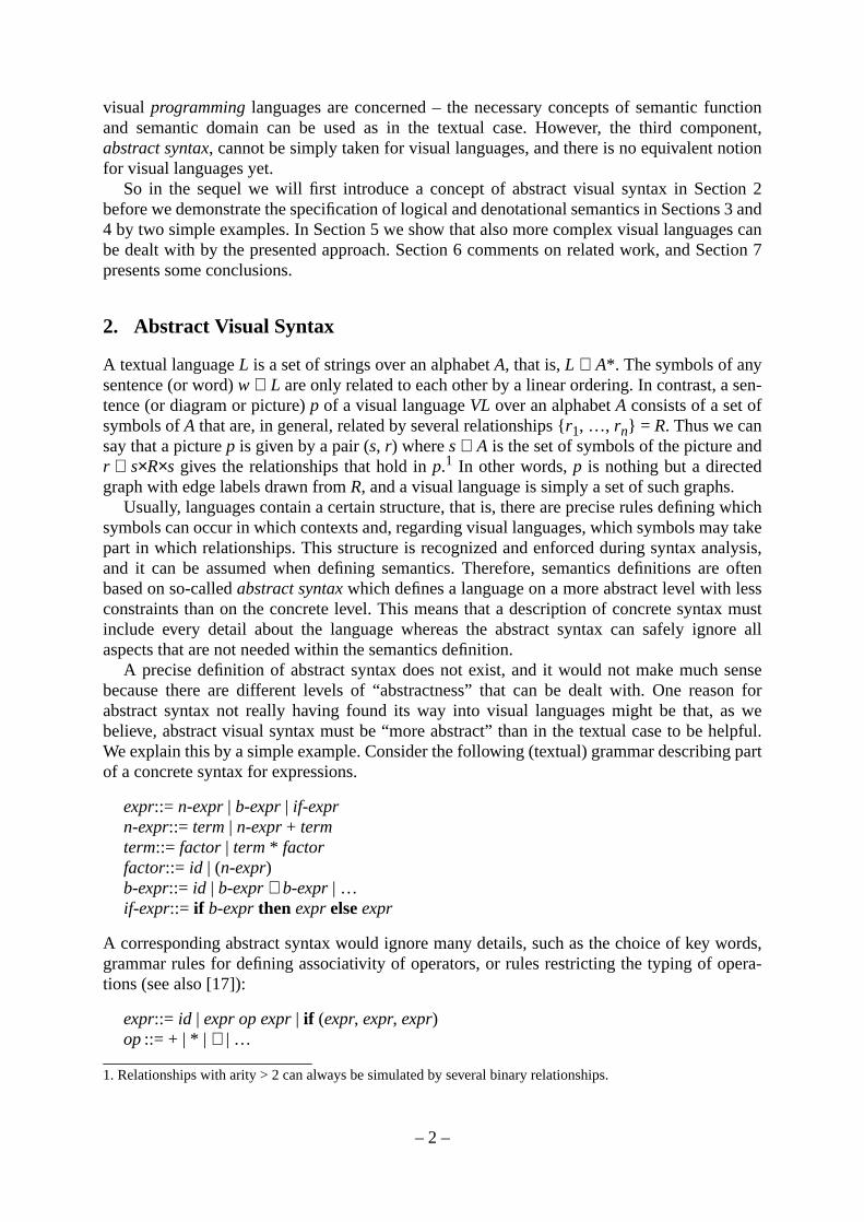
All A is B SomeC is ASomeC is B

Although this sounds very intuitive, this rule is formallynot correct since “SomeC is B” doesonly hold if C - B ≠ ∅. But this cannot be concluded from the premises;C might well beincluded inB. Actually, Euler is aware of this fact and gives pictures illustrating both cases. Thepoint is that there is no formal correspondence between propositions and pictures (since thereis no formal semantics). Now the correct rule is:

All A is B SomeC is AAll C is B or SomeC is B

or equivalently in visual terms:

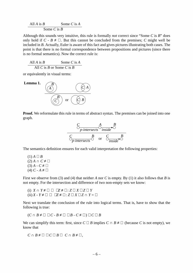
Proof. We reformulate this rule in terms of abstract syntax. The premises can be joined into onegraph.

The semantics definition ensures for each valid interpretation the following properties:

(1) A ⊆ B(2) A ∩ C ≠ ∅(3) A - C ≠ ∅(4) C - A ≠ ∅

First we observe from (3) and (4) that neitherA norC is empty. By (1) it also follows thatB isnot empty. For the intersection and difference of two non-empty sets we know:

(i) X ∩ Y ≠ ∅ ⇔ ∃Z ≠ ∅: Z ⊆ X ∧ Z ⊆ Y(ii) X - Y ≠ ∅ ⇔ ∃Z ≠ ∅: Z ⊆ X ∧ Z ∩ Y = ∅

Next we translate the conclusion of the rule into logical terms. That is, have to show that thefollowing is true:

(C ∩ B ≠ ∅ ∧ C - B ≠ ∅ ∧ B - C ≠ ∅) ∨ C ⊆ B

We can simplify this term: first, sinceC ⊆ B impliesC ∩ B ≠ ∅ (becauseC is not empty), weknow that

C ∩ B ≠ ∅ ∨ C ⊆ B ⇔ C ∩ B ≠ ∅,

AB

C A

CB

or C B

Lemma 1.

C B

or

insidep-intersectsA

Cp-intersects

Binside

C B

– 7 –

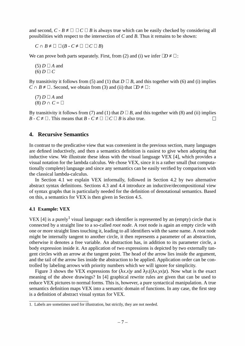
and second,C - B ≠ ∅ ∨ C ⊆ B is always true which can be easily checked by considering allpossibilities with respect to the intersection ofC andB. Thus it remains to be shown:

C ∩ B ≠ ∅ ∧ (B - C ≠ ∅ ∨ C ⊆ B)

We can prove both parts separately. First, from (2) and (i) we infer∃D ≠ ∅:

(5) D ⊆ A and(6) D ⊆ C

By transitivity it follows from (5) and (1) thatD ⊆ B, and this together with (6) and (i) impliesC ∩ B ≠ ∅. Second, we obtain from (3) and (ii) that∃D ≠ ∅:

(7) D ⊆ A and(8) D ∩ C = ∅

By transitivity it follows from (7) and (1) thatD ⊆ B, and this together with (8) and (ii) impliesB - C ≠ ∅. This means thatB - C ≠ ∅ ∨ C ⊆ B is also true.

4. Recursive Semantics

In contrast to the predicative view that was convenient in the previous section, many languagesare defined inductively, and then a semantics definition is easiest to give when adopting thatinductive view. We illustrate these ideas with the visual language VEX [4], which provides avisual notation for the lambda calculus. We chose VEX, since it is a rather small (but computa-tionally complete) language and since any semantics can be easily verified by comparison withthe classical lambda-calculus.

In Section 4.1 we explain VEX informally, followed in Section 4.2 by two alternativeabstract syntax definitions. Sections 4.3 and 4.4 introduce an inductive/decompositional viewof syntax graphs that is particularly needed for the definition of denotational semantics. Basedon this, a semantics for VEX is then given in Section 4.5.

4.1 Example: VEX

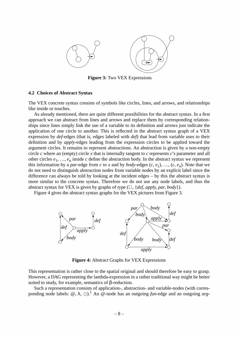
VEX [4] is a purely1 visual language: each identifier is represented by an (empty) circle that isconnected by a straight line to a so-calledroot node. A root node is again an empty circle withone or more straight lines touching it, leading to all identifiers with the same name. A root nodemight be internally tangent to another circle, it then represents a parameter of an abstraction,otherwise it denotes a free variable. An abstraction has, in addition to its parameter circle, abody expression inside it. An application of two expressions is depicted by two externally tan-gent circles with an arrow at the tangent point. The head of the arrow lies inside the argument,and the tail of the arrow lies inside the abstraction to be applied. Application order can be con-trolled by labeling arrows with priority numbers which we will ignore for simplicity.

Figure 3 shows the VEX expressions for (λx.x)y andλy.((λx.yx)z). Now what is the exactmeaning of the above drawings? In [4] graphical rewrite rules are given that can be used toreduce VEX pictures to normal forms. This is, however, a pure syntactical manipulation. A truesemantics definition maps VEX into a semantic domain of functions. In any case, the first stepis a definition of abstract visual syntax for VEX.

1. Labels are sometimes used for illustration, but strictly, they are not needed.

– 8 –

4.2 Choices of Abstract Syntax

The VEX concrete syntax consists of symbols like circles, lines, and arrows, and relationshipslike inside or touches.

As already mentioned, there are quite different possibilities for the abstract syntax. In a firstapproach we can abstract from lines and arrows and replace them by corresponding relation-ships since lines simply link the use of a variable to its definition and arrows just indicate theapplication of one circle to another. This is reflected in the abstract syntax graph of a VEXexpression bydef-edges (that is, edges labeled withdef) that lead from variable uses to theirdefinition and byapply-edges leading from the expression circles to be applied toward theargument circles. It remains to represent abstractions. An abstraction is given by a non-emptycirclec where an (empty) circlex that is internally tangent toc representsc’s parameter and allother circlese1, …, en insidec define the abstraction body. In the abstract syntax we representthis information by apar-edge fromc to x and bybody-edges (c, e1), …, (c, en). Note that wedo not need to distinguish abstraction nodes from variable nodes by an explicit label since thedifference can always be told by looking at the incident edges – by this the abstract syntax ismore similar to the concrete syntax. Therefore we do not use any node labels, and thus theabstract syntax for VEX is given by graphs of type (∅, { def, apply, par, body}).

Figure 4 gives the abstract syntax graphs for the VEX pictures from Figure 3.

This representation is rather close to the spatial original and should therefore be easy to grasp.However, a DAG representing the lambda-expression in a rather traditional way might be bettersuited to study, for example, semantics ofβ-reduction.

Such a representation consists of application-, abstraction- and variable-nodes (with corres-ponding node labels: @,λ, ).1 An @-node has an outgoingfun-edge and an outgoingarg-

Figure 3: Two VEX Expressions

Figure 4: Abstract Graphs for VEX Expressions

par

body

defapply

defpar

def

applydef

apply

defbody

par

body

body

body

– 9 –

edge that lead to the function to be applied and the argument, respectively. A λ-node is con-nected by an outgoingpar-edge to its parameter, an unlabeled node, and by an outgoingbody-edge to the node representing its body. Hence, this abstract syntax for VEX uses graphs of type({@, λ}, { fun, arg, par, body}).

Figure 5 shows the abstract syntax graphs that correspond to the VEX pictures of Figure 3.

At this point it is important to recall that the informally stated structural properties are not cap-tured by abstract syntax graphs. This means that the graph shown below is also a graph of theabove type although it is certainly not representing any VEX expression.

For defining semantics we can safely assume structurally correct graphs be delivered, say, by asyntax analysis phase or an editor. The structural assumptions can then appear implicit in thesemantics definition since we need only give semantics for structurally well-formed graphs,that is, syntactically correct pictures.

Although the second representation offers advantages in treating certain aspects of seman-tics, it does only poorly reflect the visual structure of the VEX expression, and might therebycomplicate the understanding of the originalvisual language. The decision of which represen-tation to choose depends on what is done with the semantics definition: for just giving a mean-ing to VEX pictures, the first approach might be sufficient, however, when trying to prove, forexample, soundness ofβ-reduction, or deriving an implementation, the second representationwould probably be favored.

Next we would like to define the semantics on the basis of the abstract representations justgiven. We therefore need a structured way of accessing all the elements of a syntax graph. Inparticular, we need an inductive view of graphs that allows the step-by-step decomposition ofgraphs. We will address this issue in the next two subsections. The concepts presented there canalso be used to map between different syntax representations.

4.3 An Inductive Graph Model

We can view a graph in the style of algebraic data types found in functional languages like MLor Haskell: a graph is either empty, or it is constructed by a graphg and a new nodev together

1. Note that we do not need node labels to distinguish variables. As in the previous approach, uses of variables arelinked by edges to the corresponding definitions. This mechanism is a perfect substitute for the “equal name”-method of the textual lambda-calculus. Therefore, nodes representing variables are left unlabeled.

Figure 5: Alternative Abstract Syntax Graphs for VEX

fun arg@

par bodyλ

parbodyλ

@funarg

fun arg@

parλ

body

par

arg

@

λarg

– 10 –

with edges fromv to its successors ing and edges from its predecessors ing leading tov. Thisway we can construct graph expressions with a constant constructorEmpty and a constructorNtaking as arguments a triple (pred-spec, node-spec, succ-spec), callednode context, and thegraphg to be extended. Here,node-spec is a node identifier not already contained ing possiblyfollowed by a label (for example,d:@) andpred-spec (succ-spec) denotes a list1 of predecessor(successor) nodes possibly extended by labels for the edges that come from (lead to) the nodes.For instance, [d›fun, e] denotes a list of two predecessor nodesd ande where the edge comingfrom d has labelfun and the edge coming frome has no label at all. Similarly, [par›a, body›a]denotes a single successora that is reached via two differently labeled edges.

The first graph from Figure 5 is given by the following expression:

N ([], d:@, [fun›b, arg›c]) (N ([], c, []) (N ([], b:λ, [par›a, body›a]) (N ([], a, []) Empty)))

Herea, b, c, andd are arbitrary, pairwise different node identifiers. In the sequel we make useof two abbreviations: (1) empty sequences can be omitted, and (2) a cascade ofN-constructorsis replaced by a singleN*-constructor. So the above term can be simplified to:

N* (d:@, [fun›b, arg›c]) (c) (b:λ, [par›a, body›a]) (a) Empty

Note that there are, in general, many different graph expressions denoting the same graph, forexample, the above term denotes the same graph as:

N* ([ d›fun], b:λ, [par›a, body›a]) (d:@, [arg›c]) (c) (a) Empty

The relationship between graph expressions and multi-graphs is formally defined as follows:

γ(Empty) = (∅, ∅, ∅, ∅, ∅)γ(N ([p1›x1, …, pn›xn], v:l, [y1›s1, …, ym›sm]) g) =

(V ∪ {v}, E ∪ {e1, …, en+m},ι ∪ {(e1, (p1, v)), …,(en, (pn, v)), (en+1, (v, s1)), …, (en+m, (v, sm))},ν ∪ {(v, l)}, ε ∪ {(e1, x1), …, (en, xn), (en+1, y1), …, (en+m, ym)})

where(V, E, ι, ν, ε) = γ(g), { e1, …, en+m} ∩ E = ∅, { p1, …, pn, s1, …, sm} ⊆ V, and v ∉ V

Thus, multi-graphs can serve as a kind of normal form for graph expressions. The followingresult is important, since it guarantees that any graph can be viewed inductively:

Theorem 1. Any directed labeled multi-graph can be represented by a graph expression.

The proof is given in [7]. There we also define a formal semantics of graph types and graphconstructors.

4.4 Pattern Matching on Graphs

The main use of graph constructors in the context of this paper is not to build new graphs but totake part in pattern matching on graphs. Especially useful for graphs is the concept ofactivepatterns [6]: usually, matching a pattern likeN (p, v:l, s) g to a graph expression binds the nodecontext inserted last top, v, l, s and the remaining graph tog. However, in order to move in acontrolled way through the graph, it is necessary to match the context of a specific node. This is

1. Lists offer a convenient way for dealing with multiple edges between two nodes. In this respect, bags wouldalso be fine, but lists can be sorted which simplifies the processing of, for example, successors, in a specific order.

– 11 –

possible ifv is already bound to the node to be matched. Then the context of v is bound to theremaining variables. For instance, matching the patternN (p, b:l, s) g against either graphexpression from the previous subsection results in the following bindings:

p → [d›fun], l → λ, s → [par›a, body›a], g → “g-term”

whereg-term is an arbitrary representation of the matched graph without nodeb and its inci-dent edges, for example,

“g-term” ≅ N* (d:@, [arg›c]) (c) (a) Empty)

Formally, graph pattern matching is defined on the basis of the represented multi-graphs. For agiven nodev assumeG can be written as:

G = (V+{v}, E+{e1, …, en+m},ι+{(e1, (p1, v)), …,(en, (pn, v)), (en+1, (v, s1)), …, (en+m, (v, sm))},ν+{(v, l)}, ε+{(e1, x1), …,(en, xn), (en+1, y1), …, (en+m, ym)})

whereS+T denotes disjoint set union and where the disjoint union forE is chosen maximally,that is, there is noe’ ∈ E such that there exists (e’, (x, y)) ∈ ι with x=v or y=v. Then matchingthe patternN (p, v:l, s) g to G produces the bindings:

p → [p1›x1, …, pn›xn], l → lab, s → [y1›s1, …, ym›sm], g → (V, E, ι, ν, ε)

This means that the meaning of pattern matching does not depend on the representation chosenby a particular graph expression. In other words, we have the freedom to choose graph expres-sions as we like; we make use of this later on in this paper when we apply semantics definitionsto example graphs. Then we shall choose representations that make inductive decompositionsof graphs simple so that we need neither transform graph expressions nor map them to the rep-resented multi-graphs.

Patterns can be made more selective by adding labels that must be present or by replacinglist variables by lists of a specific length. We can also ignore bindings by simply omitting thecorresponding parts of the pattern, for example, we can match the abstraction nodeb bindingthe parameter/body node top/e by using the pattern:

N (b:λ, [par›p, body›e]) g

Actually, p ande will be bound to the same node,a. Since we did not specify anything for thepredecessor list, no binding will be produced. If we wanted to ensure that the matched node hasno predecessors we would have used the patternN ([], b:λ, [par›p, body›e]) g instead. This,however, fails to match our example graph.

Cascading patterns likeN* c1 c2 … cn g can be matched against a graphG as follows: letg1,…, gn be auxiliary variables to be bound to intermediate decomposed graphs. Now first,N c1 g1 is matched againstG, and the bindings produced by this match, especially the nodebindings inc1 and the rest graphg1, are then used to matchN* c2 … cn g againstg1, that is,N c2 g2 is matched againstg1, N c3 g3 is matched againstg2, and so on, untilN cn gn is matchedagainstgn-1. Theng is bound togn. In this way, N* patterns can actually be used to conve-niently find paths (of fixed length) in the graph.

– 12 –

4.5 Denotational Semantics

Now we can define the denotational semantics of VEX. We map each syntax graph of a (syn-tactically correct) VEX expression into a value of a suitable domainD for the lambda-calculus(for example, Scott’s constructionD∞ or Plotkin’s graph modelPω [2]). Let d be a variabledenoting values fromD. It is interesting to note that in contrast to the denotational semantics ofthe textual lambda-calculus we do not need any environment for passing around variable bind-ings; we can rather employ the VEX root nodes to carry semantic values. It would be also pos-sible to map the abstract syntax to textual lambda-expression and to rely on semantics alreadydefined for the lambda-calculus. However, this would mean one further intermediate represen-tation and, as noted, a sligthly more complicated semantics definition with the need for an envi-ronment.

We define the semantics by moving in a controlled way through the abstract graph, that is,semantics are given with respect to specific node contexts in the graph, and in the recursive def-initions for the semantics of, say, nodev, the semantics functionS’ is applied to the contexts ofv’s successors. Hence,S’ has two parameters: a graph and a node determining the context.Using the second proposal for abstract syntax we can distinguish the following cases: first, thesemantics of a node carrying a semantic value is the value itself. (Such a value is assigned bythe rule for abstractions.) Second, the meaning of an application node is given by applying thesemantics of the node connected by thefun-edge, which is expected to be a function value, tothe value denoted by the argument node. Finally, the semantics of an abstraction is defined tobe a function value (Λ denotes the semantic abstraction function) which maps any valued tothe value denoted by the body of the abstraction when the parameter node is labeledd. Notethat in order to change the label of the parameter nodep to d we have to decomposep from thegraph and re-insert it with the new label and the old context (that is, with predecessorsr and nosuccessors).

S’[[ v, N (v:d) g ]] = dS’[[ v, N (v:@, [fun›f, arg›a]) g ]] = S’[[ f, g ]] (S’[[ a, g ]])S’[[ v, N* (v:λ, [par›p, body›b]) (r, p) g ]] =

Λd.S’[[ b, N (r, p:d, []) g ]]

Now the semantics of a graphG representing a VEX expression is given by applyingS’ to theroot ofG.

root(G) = {v ∈ VG | predG(v) = []}S[[ G ]] = S’[[ the(root(G)), G ]]

Here, the functionthe simply extracts the one element from a singleton set and is undefinedotherwise:the({ x}) = x.

We have given an alternative semantics definition for VEX based on the other abstract syn-tax approach in [9].

We can use the denotational semantics to “compute” the meaning for particular VEXexpressions. As an example we determine the function denoted by the second VEX picture of

– 13 –

Figure 3. For convenience we repeat the abstract syntax representation with added node identi-fiers in Figure 6 to facilitate the understanding of the following derivation.

The graph (G1) is formally defined by the following expressions. The representations are cho-sen to make subsequent pattern matching easy and to have proper bindings for remaininggraphs:

G6 = N* (6:@) EmptyG4 = N* (4:λ, [par›7, body›6]) ([6›arg], 7) G6G3 = N* (3:@, [fun›4, arg›5]) (5) G4G1 = N* (1:λ, [par›2, body›3]) ([6›fun], 2) G3

Now the meaning of the graphG1 is:

S[[ G1 ]] = S’[[ the(root(G1)), G1 ]] = S’[[ 1, G1 ]]= Λd.S’[[ 3, N ([6›fun], 2:d) G3 ]]= Λd.(S’[[ 4, N ([6›fun], 2:d) G4 ]] (S’[[ 5, N (5) G4 ]]))= Λd.(Λd’.S’[[ 6, N* ([6›arg], 7:d’) ([6›fun], 2:d) G6 ]]) ⊥)= Λd.(Λd’.S’[[ 6, N* (6:@, [fun›2, arg›7]) (2:d) (7:d’) Empty]]) ⊥)= Λd.(Λd’.(S’[[ 2, N* (2:d) (7:d’) Empty]] (S’[[ 7, N* (2:d) (7:d’) Empty]]))) ⊥)= Λd.(Λd’.(d d’) ⊥)= Λd.d ⊥

Note thatS’[[ 5, N (5) G4 ]] = ⊥ because the semantics of free variables is not defined. Thus themeaning of the VEX picture is a function that applies its argument to the undefined value.

5. A Larger Example

In this section we consider abstract syntax and semantics of a more complex visual language:Show and Tell. The language is interesting for two reasons: first, it is a member of the ratherlarge class ofdata flow languages and thus indicates how semantics could be defined for manyother visual languages. Second, it demonstrates the effective use of nested syntax graphs whichgoes beyond grammatical descriptions of visual languages.

Show and Tell (STL) [15, 14] combines data flow with the concept ofcompletion, whichmeans to fill in empty boxes in a data flow graph by either computation or database search.Computations are represented by so-calledbox-graphs, which are acyclic directed multi-graphs whose nodes are rectangles connected by arrows. A box is empty or it contains either

Figure 6: Abstract Syntax for Lambda Expressionλy.((λx.yx)z)

fun arg@

par bodyλ

parbodyλ

@funarg

1

23

4

7

5

6

– 14 –

simple data, such as numbers or functions, or another whole box-graph. In that case the box iscalledcomplex and can be eitherclosed or open. Data can flow along the arrows from one boxto another. Whenever two boxes connected by an arrow contain different values, the box-graphis said to beinconsistent. An open box containing an inconsistent box-graph propagates thisinconsistency, that is, the box-graph containing the inconsistent box also becomes inconsistent.In contrast, when a closed box gets inconsistent, all that happens is that the box cannot receiveor propagate any values, that is, an inconsistent closed box can be viewed as deleted. With theconcept of inconsistency, conditionals can be expressed without having boolean values.

Figure 7 shows an STL program implementing the logical AND.

The program contains two parameters (the two topmost empty boxes) and one result (theempty box on the left). If both arguments are “1”, then the upper (closed) complex box remainsconsistent, and the “1” can flow directly into the result box. Moreover, the lower (closed) com-plex box gets inconsistent and cannot emit the “0”. On the other hand, if one argument is “0”,then the upper complex box gets inconsistent and cannot send data to the result box and to thelower box. Then, the “0” can flow from the lower box into the result box.

We choose an abstract syntax that mainly follows the concrete syntax. In particular:

(1) Nodes are labeled by constants (for example, integers), function symbols (such as +),(representing empty STL boxes), and complete graphs. Additionally, they carry anopen-or closed-tag. (In the following we will mention these tags only when needed.)

(2) Edges are labeled by pairs (i, j) wherei means that the edge contributes to theith param-eter of the target node andj says that thejth component of the value at the edge’s sourcenode flows via this edge. Ifj=*, this means that the complete value flows via the edge.

(3) Each edgee = (v, w):(i, j) (that is, fromv to w with label (i, j)) that crosses a border of acomplex boxu is replaced by a new nodex with labelk (lying insideu) and two edgese1ande2 as follows:

(i) If w is insideu, thene1 = (v, u):(k, j) (ending atu) ande2 = (x, w):(i, *)(connectingx to the target ofe).

(ii) If v is insideu, thene1 = (v, x):(1, j) ande2 = (u, w):(i, k).Here,k ranges from 1 ton (m) for all n incoming (m outgoing) edges and represents theargument position of the node.

(4) The (top-level) box-graph is extended according to rule (3) as if it were enclosed by a(closed) box having edges ending at the roots and leaving the sinks.

The abstract syntax of the STL program from Figure 7 is show in Figure 8. For later referencewe have added small node numbers to the labels. Nodes with constants as labels are surrounded

Figure 7: STL program for Logical AND

1

0

– 15 –

by circles and can thus be distinguished from newly introduced nodes. Formally, we use inte-gers as labels of newly introduced nodes and quoted integers as constant labels. This means,the label of node 4 is 2 whereas the label of node 8 is ´1.

If OP is the set of constants and operations used by STL programs, then STL abstract graphswithout complex boxes have typeΓ(α0, β) with (let IN= {´} × IN):

α0 = (OP ∪ { } ∪ IN ∪ ´IN) × {open, closed}β = IN × (IN ∪ {*})

Since complex boxes are represented by nodes labeled with abstract STL graphs, the node typecan be inductively defined to include graphs of increasing nesting:

αi+1 = αi ∪ Γ(αi, β)

Hence, the type of arbitrary STL abstract syntax graphs is given byΓ = ∪i ≥ 0 Γ(αi, β).We can now define the semantics of each STL DAG as a functionDn → Dm when we take a

domain of semantic valuesD (for example, for integers) and add to it a special value◊ for deal-ing with inconsistency (see below). The first equation selects all roots of the graph, assignsD-variables as new labels, and yields a function over these variables:

S’[[ N* ([], v1:1, s1) … ([], vn:n, sn) g ]] =Λ(d1, …, dn).S’[[ N* ([], v1:d1, s1) … ([], vn:dn, sn) g ]]

The used cascade pattern with the ellipsis extends as far as possible, that is, it selects all nodeslabeled by integers and having no predecessors. The recursive application ofS’ denotes theresult tuple (by applying another semantic functionS’’ to all sinks of the graph) together withthe consistency status of the whole graph given byC.

S’[[ N* ([ p1], v1:1, []) … ([pm], vm:m, []) g ]] = ((S’’[[ p1, g ]], …, S’’[[ pm, g ]]), C[[ g ]])

(Note that by definition of abstract syntax each sink has exactly one predecessor.) S’’ moves inreverse direction through the abstract graph: it recursively determines the tuple of values for all

Figure 8: Abstract Syntax of the STL Program

1 2

12

12

1(1,*)

(2,*)

(1,*)(1,*)

1

1

(1,*)

(1,*)

1

(1,*) (2,*)

(1,*) (1,*)

(1,2)

(1,1)

(2,1)

(1,*)

0

1 2 3 4

56

7

8

910

11 12

13

14

15

16

– 16 –

predecessors and applies the function denoted by the current node to it. This function isdenoted by the semantic functionF defined below. In the pattern we assume that the predeces-sors (pi) are ordered with respect to the first label component (i) of the connecting edges. Thisensures that the parameters appear in the correct order. Note that the values of the predecessorsare not taken as a whole, but only the specific components as specified by the second label part(si) of the connecting edges. This is achieved by the application of projecting functionsΠsi(whereΠ*(x) = x).

S’’[[ v, N ([p1›(1, s1), …, pk›(k, sk)], v:f) g ]] = F[[ f ]] (Πs1(S’’[[ p1, g ]]), …, Πsk(S’’[[ pk, g ]]))

The semantic functionsS’ andS’’ only define the meaning of consistent STL-graphs. An incon-sistent node or graph is defined to return the value◊ which is defined to be equal to all othervalues ofD. In this way, an inconsistent (closed) node that is connected by an edge to a nodevthat is labeled by a constant or not labeled at all does not affect the result ofv. A graph is incon-sistent if any of its open nodes is inconsistent. Letopen be a predicate that is true only for opennodes. The consistency of nodes/graphs is denoted byC’/C:

C’[[ v, G ]] = (open(v) ⇒ S’’[[ v, G ]] ≠ ◊)C[[ G ]] = ∀v ∈ VG: C’[[ v, G ]]

Now the semantics of an STL graph is finally given by:

Π1(S’[[ G ]]) if Π2(S’[[ G ]])S[[ G ]] =

◊ otherwise

If G contains no open boxes, the propagation of inconsistency need not be taken into accountbecause in that caseC’ and C always yieldtrue. Thus the semantics for graphs without openboxes simplifies to:

S[[ G ]] = S’[[ G ]]S’[[ N* ([ p1], v1:1, []) … ([pm], vm:m, []) g ]] = (S’’[[ p1, g ]], …, S’’[[ pm, g ]])

It remains to define the functions denoted by node labels. An operation onD (like +) denotesitself. A constantc is interpreted as a function that checks whether all incoming values areequal toc, and an unlabeled node checks all incoming values for equality. Finally, the seman-tics of a node labeled by a complete STL graph is given byS.

F[[ f : Dn → Dm ]] = fF[[ c : D ]] = Λ(d1, …, dn).if d1=…=dn=c then c else ◊F[[ ]] = Λ(d1, …, dn).if d1=…=dn then d1 else ◊F[[ G : Γ ]] = S[[ G ]]

The first line includes the case for constant labels, that is,n=0. This means in particular, that thedefinition ofS’’ reduces in this special case to:

S’’[[ v, N ([p1›(1, s1), …, pk›(k, sk)], v:d) g ]] = d

In the reminder of this section we demonstrate the semantics definition by proving the correct-ness of the STL program of Figure 7, that is, we want to show that the program indeed com-putes the logical AND. LetG be any graph expression representing the abstract syntax graphshown in Figure 8. Then we have to prove:

– 17 –

Theorem 2. S[[ G ]] = Λ(d1, d2).if d1=d2=1 then 1 else 0.

Proof. We use the following abbreviations:

G|v1:l1,…,vn:ln :=if G = N* (p1, v1, s1) … (pn, vn, sn) G’ then N* (p1, v1:l1, s1) … (pn, vn:ln, sn) G’ else ⊥

eq := Λ(d1, …, dn).if d1=…=dn then d1 else ◊eqc := Λ(d1, …, dn).if d1=…=dn=c then c else ◊

SinceG contains no open boxes we can work with the simplified semantics, that is,S[[ G ]] =S’[[ G ]]. Thus:

S[[ G ]] = S’[[ G ]]= S’[[ N* ([], 1:1, [(1,*)›2]) ([], 4:2, [(1,*)›3]) g ]]= Λ(d1, d2).S’[[ G|1:d1,4:d2 ]] (= Λ(d1, d2).S’[[ N* ([],1:d1,[(1,*)›2]) ([],4:d2,[(1,*)›3]) g ]])= Λ(d1, d2).S’[[ N ([12›(1,*)], 11:1, [])g11]]

Again we can ignoreC and use the simplified definition forS’’. Thus we can continue (omittingbrackets around the one-tuple):

= Λ(d1, d2).S’’[[ 12,g11]]= Λ(d1, d2).S’’[[ 12,N ([5›(1,1), 13›(2,1)], 12: ) g12]]= Λ(d1, d2).F[[ ]] (Π1(S’’[[ 5, g12]]), Π1(S’’[[ 13,g12]])) (A)

We next have to determineS’’[[ 5, g12]] andS’’[[ 13,g12]].

S’’[[ 5, g12]]= S’’[[ 5, N ([2›(1,*), 3›(2, *)], 5:G5) g5 ]]= F[[ G5 ]] (Π* (S’’[[ 2, g5 ]]), Π* (S’’[[ 3, g5 ]]))= S[[ G5 ]] (S’’[[ 2, g5 ]], S’’[[ 3, g5 ]]) (B)

To proceed we now needS’’[[ 2, g5 ]], S’’[[ 3, g5 ]], andS[[ G5 ]]. Note in the following thatg5 andthus all reduced graphs derived from that have their origin in the graphG|1:d1,4:d2, that is,nodes 1 and 4 have assigned the semantic values (variables)d1 andd2.

S’’[[ 2, g5 ]]= S’’[[ 2, N ([1›(1,*)], 2: ) g2 ]]= F[[ ]] (Π* (S’’[[ 1, g2 ]]))= eq (S’’[[ 1, N (1:d1) g1 ]])= eq (d1)= d1

The derivation forS’’[[ 3, g5 ]] is almost identical and yields:

S’’[[ 3, g5 ]] = d2

For S[[ G5 ]] we obtain:

– 18 –

S[[ G5 ]] = S’[[ G5 ]]= S’[[ N* ([], 6:1, [(1,*)›8]) ([], 7:2, [(2,*)›8]) g’ ]]= Λ(d3, d4).S’[[ G5|6:d3,7:d4 ]]= Λ(d3, d4).S’[[ N* ([8›(1,*)], 9:1, []) ([8›(1,*)], 10:2, []) g9 ]]= Λ(d3, d4).(S’’[[ 8, g9 ]], S’’[[ 8, g9 ]])

In the next two lines we give only the values for the first component of the pair, since the sec-ond component is identical.

= Λ(d3, d4).(S’’[[ 8, N ([6›(1,*), 7›(2,*)], 8:´1)g8 ]], …)= Λ(d3, d4).(F[[ 8:´1]](Π* (S’’[[ 6, g8 ]]), Π* (S’’[[ 7, g8 ]])), …)= Λ(d3, d4).(eq1(d3, d4), eq1(d3, d4))

We can insert the results forS’’[[ 2, g5 ]], S’’[[ 3, g5 ]], andS[[ G5 ]] into (B) and obtain:

S’’[[ 5, g12]]= Λ(d3, d4).(eq1(d3, d4), eq1(d3, d4)) (d1, d2)= (eq1(d1, d2), eq1(d1, d2))

Next we determineS’’[[ 13,g12]]. This works analogous to the derivation ofS’’[[ 5, g12]]. Sinceg13 is different formg12, we formally have to derive S’’[[ 5, g13]] from anew, but it is obviousthat it results in the same function asS’’[[ 5, g12]]. So we get:

S’’[[ 13,g12]]= S’’[[ 13,N ([5›(1,2)], 13:G13) g13]]= F[[ G13]] (Π2(S’’[[ 5, g13]]))= Λd5.eq0(d5) (eq1(d1, d2))= eq0(eq1(d1, d2))= if d1=d2=1 then ◊ else 0

To understand the last step consider two cases: ifd1=d2=1, theneq1(d1, d2) = 1, andeq0(1) =◊.Otherwise,eq1(d1, d2) = ◊, and since◊ is equal to all values,eq0(◊) = 0.

Finally, we can insertS’’[[ 5, g12]] andS’’[[ 13,g12]] into (A) and we obtain (note thatΠ1 hasno effect on a one-tuple):

S[[ G ]] == Λ(d1, d2).F[[ ]] (Π1(S’’[[ 5, g12]]), Π1(S’’[[ 13,g12]]))= Λ(d1, d2).eq (eq1(d1, d2), if d1=d2=1 then ◊ else 0)= Λ(d1, d2).if d1=d2=1 then 1 else 0

Again, to understand the last step consider the following two cases:

(1) If d1=d2=1, theneq1(d1, d2) = 1 and the second expression yields◊. Thus the argumentpair ofeq is (1,◊), andeq(1, ◊) = 1.

(2) If d1≠1 or d2≠1, theneq1(d1, d2) = ◊, but now the second expression yields 0. Thus theargument pair ofeq is (◊, 0), andeq(◊, 0) = 0.

This completes the proof.

– 19 –

6. Related Work

6.1 Syntax of Visual Languages

There has been quite a lot of work concerning the syntax of visual languages, for an overview,see [16]. However, all these formalisms are concerned with the specification of concrete syntaxand address the related aspects of parsing and syntax directed editors.

Only few papers deal with abstract visual syntax. In [1, 18, 19] the authors recommend theseparation of abstract syntax from concrete syntax. However, this is only partially achieved bythose approaches, since they require a one-to-one correspondence between concrete andabstract syntax, and thus abstract syntax is intrinsically coupled very closely to concrete syn-tax. Also, that work is only concerned with translation of visual languages, aspects of seman-tics definitions are not discussed. More on abstract visual syntax as used in this paper can befound in [8].

6.2 Semantics of Visual Languages

Besides semantics definitions for specific languages, such as [14], there has been not muchdone about semantics of visual languages in general. Wang and Lee [21] take an algebraic viewof modeling pictures. Their goal is to get a formal basis for visual reasoning by axiomatic char-acterizations of what can be seen in a picture. The work of Bottoni et al. [3] is centered aroundthe formal understanding of and reasoning with images. Both approaches are based on concretevisual syntax and are not targeted at the semantics specification of visualprogramming lan-guages.

The term “semantics” is sometimes used with a different meaning, for example, in [13] itmeans a set of pictures satisfying a given specification, that is, the semantics is a visual lan-guage itself and not a mathematical domain describing the computations performed by a visuallanguage.

6.3 Graph Representation

Using graphs to describe pictures is a common and wide-spread approach. However, generalmodels that apply to a broad range of visual languages are few. Examples are Harel’s higraphs[12] and the theory of graph grammars [5].

Higraphs are a kind of amalgam of hierarchical graphs and Euler/Venn diagrams. Higraphshave a concise formal semantics, and by modeling a visual languageVL as a higraph, thesemantics ofVL is implicitly defined. Higraphs provide a perfect representation for those visuallanguages that exactly fit that model. However, since higraphs have a fixed structure, theirapplicability is restricted, and only a certain class of visual languages can be expressed in termsof them. Hence, although quite many applications can, in principal, be described as higraphs,several of them require changes of their concrete syntax, and some languages cannot bedescribed at all. Moreover, the lack of an inductive view of higraphs makes denotational speci-fications difficult, if not impossible.

Graph grammars, on the other hand, provide a fairly general model of visual languages.Graph grammars are very powerful, and they have been extensively used to describe graphtransformations. Graph grammars enjoy a large body of theoretical results, and they also pro-vide, in a certain sense, an inductive view of graphs. So why should we need yet another graphmodel? A major difficulty with graph grammars is that they consider the graphs they operate on

– 20 –

as global variables that can be updated destructively. This means that changes performed bygrammar rules are implicitly propagated, and thus a declarative treatment of graphs is prohib-ited. Things are complicated by the fact that the semantics of graph grammars themselves israther complex due to advanced embedding rules and nondeterminism. In contrast, the induc-tive graph view presented in this paper is quite simple, and it treats graphs as explicit parame-ters of transformations.

7. Conclusions and Future Work

We have presented a general framework for the specification of visual language semantics. Arather unrestricted form of abstract visual syntax given by graphs is the backbone of the for-malism. The approach applies to quite a wide range of visual languages, and we can evenemploy different semantics formalism, such as denotational or logical semantics.

A drawback of the approach presented so far is that visual information is mapped com-pletely to a textual description. We are currently extending the formalism by a heterogeneous,that is, semi-visual, notation so that certain relationships, such as adjacency or intersection,need not be encoded in graph edges, but can be kept in visual form [9]. This will make seman-tics definitions and other transformations much more readable.

8. References

1. M. Andries, G. Engels & J. Rekers (1996) How to Represent a Visual Program?Workshopon Theory of Visual Languages. Boulder, Colorado.

2. H.P. Barendregt (1981)The Lambda Calculus – Its Syntax and Semantics, North Holland,Amsterdam, 615 pp.

3. P. Bottoni, M.F. Costabile, S. Levialdi & P. Mussio (1995) Formalising Visual Languages.IEEE Symp. on Visual Languages. Darmstadt, Germany, pp. 45-52.

4. W. Citrin, R. Hall & B. Zorn (1995) Programming with Visual Expressions.IEEE Symp. onVisual Languages. Darmstadt, Germany, pp. 294-301.

5. B. Courcelle (1990) Graph Rewriting: An Algebraic and Logic Approach. In:Handbook ofTheoretical Computer Science, Vol. B (J. van Leeuwen, ed.) Elsevier, Amsterdam, pp. 193-242.

6. M. Erwig (1996) Active Patterns.8th Int. Workshop on Implementation of Functional Lan-guages. Bonn, Germany, LNCS 1268, pp. 21-40.

7. M. Erwig (1997) Functional Programming with Graphs. 2nd ACM SIGPLAN Int. Conf. onFunctional Programming. Amsterdam, The Netherlands, pp. 52-65.

8. M. Erwig (1997) Abstract Visual Syntax. 2nd IEEE Int. Workshop on Theory of Visual Lan-guages. Capri, Italy, pp. 15-25.

9. M. Erwig (1998) Visual Semantics – Or: What You See is What You Compute.IEEE Symp.on Visual Languages. Halifax, Nova Scotia, to appear.

10. M. Erwig & B. Meyer (1995) Heterogeneous Visual Languages – Integrating Visual andTextual Programming.IEEE Symp. on Visual Languages. Darmstadt, Germany, pp. 318-325.

– 21 –

11. L. Euler (1986)Briefe an eine deutsche Prinzessin. Vieweg, Germany.

12. D. Harel (1988) On Visual Formalisms.Communications of the ACM 31(5), 514-530.

13. R. Helm & K. Marriott (1991) A Declarative Specification and Semantics for Visual Lan-guages.Journal of Visual Languages and Computing 2, 311-331.

14. T.D. Kimura (1986) Determinacy of Hierarchical Dataflow Model. Report WUCS-86-5,Washington University, St. Louis.

15. T.D. Kimura, J.W. Choi & J.M. Mack (1990) Show and Tell: A Visual Programming Lan-guage. In:Visual Programming Environments (E.P. Glinert, ed.) IEEE Computer SciencePress, Los Alamitos/CA, pp. 397-404.

16. K. Marriott, B. Meyer & K. Wittenburg (1996) A Survey of Visual Language Specificationand Recognition.Workshop on Theory of Visual Languages, Boulder, Colorado.

17. P.D. Mosses (1990) Denotational Semantics. In:Handbook of Theoretical Computer Sci-ence, Vol. B (J. van Leeuwen, ed.) Elsevier, Amsterdam, pp. 575-631.

18. J. Rekers & A. Schürr (1995) A Graph Grammar Approach to Graphical Parsing.IEEESymp. on Visual Languages. Darmstadt, Germany, pp. 195-202.

19. J. Rekers & A. Schürr (1996) A Graph Based Framework for the Implementation of VisualEnvironments.IEEE Symp. on Visual Languages. Boulder, Colorado.

20. S.-J. Shin (1994)The Logical Status of Diagrams. Cambridge University Press, New York,197 pp.

21. D. Wang & J.R. Lee (1993) Visual Reasoning: its Formal Semantics and Applications.Journal of Visual Languages and Computing 4, 327-356.