ABSTRACT

Title of dissertation: SYNCHRONIZATION AND PREDICTIONOF CHAOTIC DYNAMICS ON NETWORKSOF OPTOELECTRONIC OSCILLATORS

Adam Brent Cohen, Doctor of Philosophy, 2011

Dissertation directed by: Professor Rajarshi RoyDepartment of Physics

The subject of this thesis is the exploration of chaotic synchronization for

novel applications including time-series prediction and sensing. We begin by char-

acterizing the nonlinear dynamics of an optoelectronic time-delayed feedback loop.

We show that synchronization of an accurate numerical model to experimental mea-

surements provides a way to assimilate data and forecast the future of deterministic

chaotic behavior. Next, we implement an adaptive control method that maintains

isochronal synchrony for a network of coupled feedback loops when the interaction

strengths are unknown and time-varying. Control signals are used as real-time esti-

mates of the variations present within the coupling paths. We analyze the stability

of synchronous solutions for arbitrary coupling topologies via a modified master

stability function that incorporates the adaptation response dynamics. Finally, we

show that the master stability function, which is derived from a set of linearized

equations, can also be experimentally measured using a two-node network, and it

can be applied to predict the convergence behavior of large networks.

SYNCHRONIZATION AND PREDICTIONOF CHAOTIC DYNAMICS ON NETWORKSOF OPTOELECTRONIC OSCILLATORS

by

Adam Brent Cohen

Dissertation submitted to the Faculty of the Graduate School of theUniversity of Maryland, College Park in partial fulfillment

of the requirements for the degree ofDoctor of Philosophy

2011

Advisory Committee:Professor Rajarshi Roy, Chair/AdvisorProfessor Thomas E. MurphyProfessor Brian R. HuntProfessor Edward OttDr. Louis M. Pecora

c⃝ Copyright byAdam Brent Cohen

2011

Goethe tells us in his greatest poem that Faust lost the liberty of his

soul when he said to the passing moment: “Stay, thou art so fair.” And

our liberty, too, is endangered if we pause for the passing moment, if we

rest on our achievements, if we resist the pace of progress. For time and

the world do not stand still. Change is the law of life. And those who

look only to the past or the present are certain to miss the future.

–John F. Kennedy

ii

Acknowledgments

The main lesson of my graduate studies is that nonlinear dynamics prevails in

areas well beyond the physics laboratory. My own state is the result of a complex

intermingling of personal interactions, sometimes harmonizing into a shared con-

sciousness but more often as a mixture of disconnected, incoherent, or contradictory

ideas. This thesis is a testament to a complicated set of interactions of thoughts,

experiences, and – above all – people that, when combined, have lead to something

much more than the sum of its parts.

Rajarshi Roy and Thomas Murphy helped identify challenging problems for

which even partial solutions expose insights about the essence of synchronization.

To seek experiments whose outcomes cast a breadth of implications and which open

a new set of questions defines the objective of a good scientist, for which both Raj

and Tom are exemplary.

Bhargava Ravoori has been a close collaborator and friend whose ideas have

shaped the evolution of the projects contained within this thesis as well as my

development into the scientist and man I am today. We have literally traveled the

world together and share an unforgettable set of experiences and emotions.

I have been fortunate to have productive collaborations with many scientists,

including: Gilad Barlev, Xiaowen Li, Adilson Motter, Edward Ott, John Rodgers,

Karl Schmitt, Anurag Setty, Francesco Sorrentino, Jie Sun, and Caitlin Williams.

I am grateful for my scientific and personal interactions with: Stanislaw An-

tol, Elizabeth Dakin, Syamal Dana, Hien Dao, Aaron Hagerstrom, Rachel Kramer,

iii

Nicholas Mecholsky, Julia Salevan, Ira Schwartz, Abhijit Sen, Gautam Sethia, and

Jordi Zamora-Munt.

I thank Yanne Chembo Kouomo, Xiaowen Li, Elbert Macau, and Francesco

Sorrentino for their time and efforts in carefully reading and thoughtfully comment-

ing on early drafts of this document. Their advice is responsible for much of its

clarity. However, any errors, omissions, and inconsistencies are entirely my own.

I cannot relate the successes of my graduate studies without highlighting the

interactions I have had at the three Hands-On Research Schools for Complex Sys-

tems in: Gandhinagar, India; Sao Paulo, Brazil; and Buea, Cameroon. All the

participants have been a source of motivation and excitement for my research and

for my interests and goals outside of academia. I am grateful to Harry Swinney,

Kenneth Showalter, and Rajarshi Roy for their tireless dedication to the School.

Harry has been especially inspirational with his mission for low-cost, high reward

science.

Finally, I am forever indebted to Rebecca Schofield for her ceaseless encour-

agement, support, and friendship.

To plot the course of my future is impossible, but the structure of my attractor

has been shaped by these interactions.

iv

Table of Contents

List of Figures vii

1 Introduction 11.1 Overview . . . . . . . . . . . . . . . . . . . . . . . . . . . . . . . . . . 11.2 Time-delayed nonlinear dynamics . . . . . . . . . . . . . . . . . . . . 31.3 Synchronization of networks of chaotic oscillators . . . . . . . . . . . 51.4 Data assimilation and time-series prediction . . . . . . . . . . . . . . 71.5 Adaptive synchronization and sensor networks . . . . . . . . . . . . . 101.6 Master stability function formulation . . . . . . . . . . . . . . . . . . 121.7 Optimal synchronizability and convergence rates . . . . . . . . . . . . 151.8 Outline of thesis . . . . . . . . . . . . . . . . . . . . . . . . . . . . . . 18

2 Components of an optoelectronic feedback loop 212.1 Qualitative description of feedback loop components . . . . . . . . . . 212.2 Semiconductor laser diode . . . . . . . . . . . . . . . . . . . . . . . . 242.3 Single-mode optical fiber . . . . . . . . . . . . . . . . . . . . . . . . . 272.4 Fiber polarization controller . . . . . . . . . . . . . . . . . . . . . . . 292.5 Mach-Zehnder intensity modulator . . . . . . . . . . . . . . . . . . . 302.6 Photodetection . . . . . . . . . . . . . . . . . . . . . . . . . . . . . . 342.7 Electronic amplification . . . . . . . . . . . . . . . . . . . . . . . . . 352.8 Electronic bandpass filter . . . . . . . . . . . . . . . . . . . . . . . . . 382.9 Time delay . . . . . . . . . . . . . . . . . . . . . . . . . . . . . . . . 412.10 Continuous-time delay differential equation model . . . . . . . . . . . 432.11 Discrete-time map equation model . . . . . . . . . . . . . . . . . . . . 472.12 Summary . . . . . . . . . . . . . . . . . . . . . . . . . . . . . . . . . 49

3 Optoelectronic chaotic dynamics 503.1 Route to chaos . . . . . . . . . . . . . . . . . . . . . . . . . . . . . . 503.2 Measures of complexity . . . . . . . . . . . . . . . . . . . . . . . . . . 59

3.2.1 Maximal Lyapunov exponent . . . . . . . . . . . . . . . . . . 593.2.2 Spectrum of Lyapunov exponents . . . . . . . . . . . . . . . . 633.2.3 Lyapunov dimension . . . . . . . . . . . . . . . . . . . . . . . 653.2.4 Kolmogorov-Sinai entropy . . . . . . . . . . . . . . . . . . . . 673.2.5 Information entropy . . . . . . . . . . . . . . . . . . . . . . . 69

3.3 Summary . . . . . . . . . . . . . . . . . . . . . . . . . . . . . . . . . 70

4 Using synchronization for time-series prediction 714.1 Open loop synchronization . . . . . . . . . . . . . . . . . . . . . . . . 724.2 Time-series prediction . . . . . . . . . . . . . . . . . . . . . . . . . . 774.3 Prediction horizon times and distribution of finite time Lyapunov

exponents . . . . . . . . . . . . . . . . . . . . . . . . . . . . . . . . . 824.4 Alternative methods for measuring phase space divergence from time-

series . . . . . . . . . . . . . . . . . . . . . . . . . . . . . . . . . . . . 86

v

4.5 Measured maximal Lyapunov exponents . . . . . . . . . . . . . . . . 894.6 Prediction using a secondary experimental system . . . . . . . . . . . 904.7 Summary . . . . . . . . . . . . . . . . . . . . . . . . . . . . . . . . . 93

5 Anticipated synchronization 945.1 Anticipated synchronization between three optoelectronic feedback

loops . . . . . . . . . . . . . . . . . . . . . . . . . . . . . . . . . . . . 965.2 Anticipated synchronization of experimental time-series by cascaded

numerical models . . . . . . . . . . . . . . . . . . . . . . . . . . . . . 1015.3 Summary . . . . . . . . . . . . . . . . . . . . . . . . . . . . . . . . . 105

6 Stability of adaptive synchronization 1066.1 Review of adaptive synchronization strategy . . . . . . . . . . . . . . 1086.2 Stability analysis of adaptive networks . . . . . . . . . . . . . . . . . 1126.3 Range of stability for adaptive three-node network . . . . . . . . . . . 1176.4 Numerical experiments of a 25-node network . . . . . . . . . . . . . . 1206.5 Symmetries of master stability function . . . . . . . . . . . . . . . . . 1226.6 Summary . . . . . . . . . . . . . . . . . . . . . . . . . . . . . . . . . 127

7 Prediction of network convergence rate 1287.1 Network convergence . . . . . . . . . . . . . . . . . . . . . . . . . . . 1297.2 Transverse Lyapunov exponents . . . . . . . . . . . . . . . . . . . . . 1317.3 Measured master stability function . . . . . . . . . . . . . . . . . . . 1357.4 Optimal synchronization . . . . . . . . . . . . . . . . . . . . . . . . . 1387.5 Estimating convergence rate from master stability function . . . . . . 1407.6 Summary . . . . . . . . . . . . . . . . . . . . . . . . . . . . . . . . . 144

8 Conclusion 1458.1 Proposed research topics . . . . . . . . . . . . . . . . . . . . . . . . . 146

8.1.1 Random number generation . . . . . . . . . . . . . . . . . . . 1468.1.2 Network reconstruction . . . . . . . . . . . . . . . . . . . . . . 1478.1.3 Master stability function symmetries . . . . . . . . . . . . . . 148

Bibliography 149

vi

List of Figures

2.1 Schematic of an optoelectronic feedback loop . . . . . . . . . . . . . . 222.2 Laser diode output power vs. drive current . . . . . . . . . . . . . . . 262.3 Mach-Zehnder optical intensity modulator . . . . . . . . . . . . . . . 312.4 Mach-Zehnder modulator transfer function . . . . . . . . . . . . . . . 332.5 Mach-Zehnder modulator extinction characteristics . . . . . . . . . . 342.6 Feedback frequency characteristics without bandwidth limitation . . . 362.7 Butterworth filter circuit diagrams . . . . . . . . . . . . . . . . . . . 382.8 Butterworth bandpass filter transfer function . . . . . . . . . . . . . . 392.9 Butterworth filter step response . . . . . . . . . . . . . . . . . . . . . 402.10 Schematic of an optoelectronic feedback loop with digital signal pro-

cessor board . . . . . . . . . . . . . . . . . . . . . . . . . . . . . . . . 422.11 Mathematical block diagram for feedback loop model . . . . . . . . . 452.12 Simulink block diagram for feedback loop . . . . . . . . . . . . . . . . 462.13 Mathematical block diagram for discrete-time feedback loop model . . 48

3.1 Experimental and simulated time series . . . . . . . . . . . . . . . . . 513.2 Experimental and simulated bifurcation diagrams . . . . . . . . . . . 523.3 Experimental and simulated frequency spectra . . . . . . . . . . . . . 543.4 PSD with noise-like features . . . . . . . . . . . . . . . . . . . . . . . 553.5 Autocorrelation functions . . . . . . . . . . . . . . . . . . . . . . . . 563.6 Time-delay embeddings . . . . . . . . . . . . . . . . . . . . . . . . . . 573.7 Chaotic time-series from DSP-based feedback loop . . . . . . . . . . . 593.8 Maximal Lyapunov exponent computation . . . . . . . . . . . . . . . 613.9 Maximal Lyapunov exponent computed for increasing feedback strengths 633.10 Lyapunov spectrum for β = 4 . . . . . . . . . . . . . . . . . . . . . . 653.11 Calculated Lyapunov dimension DL as a function of feedback strength β 663.12 Calculated KS entropy as a function of feedback strength β . . . . . . 673.13 Shannon entropy HS as a function of feedback strength . . . . . . . . 69

4.1 Simulink block diagram for open loop synchronization and time seriesprediction . . . . . . . . . . . . . . . . . . . . . . . . . . . . . . . . . 73

4.2 Open loop synchronization transient response . . . . . . . . . . . . . 744.3 Open loop synchronization error as a function of simulation parameters 754.4 Time-series prediction for non-chaotic trajectories. . . . . . . . . . . . 784.5 Time-series prediction for chaotic trajectories. . . . . . . . . . . . . . 794.6 Synchronization plots during open loop synchronization and divergence 804.7 Distribution of prediction horizon times for β = 4.0 . . . . . . . . . . 834.8 Distribution of divergence rates for different fitting intervals from

continuous-time model . . . . . . . . . . . . . . . . . . . . . . . . . . 844.9 Distribution of divergence rates for different fitting intervals from

discrete-time model . . . . . . . . . . . . . . . . . . . . . . . . . . . . 854.10 Extracting divergence rate h1 from a pair of time-series . . . . . . . . 874.11 Comparison of extracted divergence rates h1 using different methods . 89

vii

4.12 Average divergence rate h1 vs. feedback strength β . . . . . . . . . . 904.13 Schematic for synchronization-release experiment . . . . . . . . . . . 914.14 Divergence of two experimental systems . . . . . . . . . . . . . . . . . 92

5.1 Schematic of three-node anticipated synchronization experiment . . . 985.2 Anticipated time-series . . . . . . . . . . . . . . . . . . . . . . . . . . 995.3 Cross-correlation functions . . . . . . . . . . . . . . . . . . . . . . . . 1005.4 Shifted anticipated time-series . . . . . . . . . . . . . . . . . . . . . . 1005.5 Synchronization plots . . . . . . . . . . . . . . . . . . . . . . . . . . . 1015.6 Block diagram for a numerical model that anticipates an experimental

time-series. . . . . . . . . . . . . . . . . . . . . . . . . . . . . . . . . 1025.7 Anticipated synchronization of experimental data by a computer model103

6.1 Experimental schematic of three-node network of optoelectronic feed-back loops. . . . . . . . . . . . . . . . . . . . . . . . . . . . . . . . . 111

6.2 Master stability surface M(λ, z0) for z0 = 0.99. . . . . . . . . . . . . . 1166.3 Master stability function for z0 = 0.95 and z0 = 0.99 . . . . . . . . . . 1176.4 Synchronization error as A12 is scanned . . . . . . . . . . . . . . . . . 1186.5 Stability of N = 25 node network . . . . . . . . . . . . . . . . . . . . 1216.6 Master stability function M(λ) . . . . . . . . . . . . . . . . . . . . . 1226.7 M(λ) along different lines. . . . . . . . . . . . . . . . . . . . . . . . . 1236.8 Stability contours M(λ, z0) = 0 for different values of z0. . . . . . . . 1246.9 Stability radius of M as z0 is varied . . . . . . . . . . . . . . . . . . . 125

7.1 Convergence rate from experimental time-series . . . . . . . . . . . . 1307.2 Distribution of finite time transverse Lyapunov exponents . . . . . . . 1327.3 Distribution of finite time transverse Lyapunov exponents for two-

node network . . . . . . . . . . . . . . . . . . . . . . . . . . . . . . . 1337.4 Measured master stability function from two-node network . . . . . . 1377.5 Convergence properties of 50-node optimal and suboptimal networks . 1397.6 Comparison of convergence rates for 50-node network . . . . . . . . . 1427.7 Comparison of convergence rates for four-node network . . . . . . . . 143

viii

Chapter 1

Introduction

1.1 Overview

Modern progress in nonlinear science is primarily due to an interplay between

laboratory experiments, mathematical analysis, and computer simulations. Due to

this complementary and multifaceted approach, we are in a position to harness the

complexity and richness intrinsic to chaotic motion towards powerful and practi-

cal applications. We may also begin to answer fundamental questions regarding

the emergence of collective behavior between coupled oscillators in which a large

number of components evolve in a complicated interdependent choreography. The

phenomenon of synchronization, in which temporal order reigns over the competing

divergent force of chaos, is the link that connects these pursuits [1]. An understand-

ing of how one specific type of network of interacting chaotic systems can evolve in

unison, as a consequence of each individual member adjusting its internal rhythm,

can guide our scientific inquiry and may lead to the development of a variety of

applications.

To this aim, we study the nonlinear dynamics of a network of time-delayed

optoelectronic feedback loop oscillators. The individual components that comprise

each loop are reliable and robust photonic devices (including a semiconductor laser

diode, fiber optic cables, an optical intensity modulator, a photoreceiver, and ana-

1

log and digital electronics). These widely-available building blocks are connected in

an uncommon architecture in order to generate a wide range of outputs as system

parameters are adjusted. The dynamical behaviors range from periodic oscillations

to high bandwidth deterministic chaos with varying degrees of complexity and mul-

tiple time-scales [2]. This system is a good testbed for experiments on the nature

of synchronization as well as a candidate for practical implementations such as for

secure communication [3, 4], sensor networks [5], ultra-wideband waveform gener-

ation [6], and random number generation [7]. By combining elements from optics

and electronics, this setup is easily scalable, modular, and flexible. Utilization of

real-time digital signal processing within the feedback structure further enhances

the controllability of parameters and reproducibility of experimental conditions [8].

A physical model based on delay differential equations displays excellent agreement

with experimental observations [9, 10].

This thesis presents results from three projects. A common theme is the

employment of experiments and modeling, in concert, to provide new insights into

the nature of chaos and chaotic synchronization with a focus on designing proof-of-

principle realizations for novel applications. In the first project, we explore a method

based on chaotic synchrony for assimilating limited experimental observations into a

computer model to measure system parameters, estimate the current state, forecast

the future trajectory, and quantify local predictability. In the second project, we

examine the stability of synchronization on an adaptive network with time-evolving

coupling strengths and a finite response time. A mathematical formulation reduces

this high dimensional stability analysis to a low dimensional problem. In the third

2

project, we investigate the role of network structure on the robustness of synchronous

behavior. A metric based on transient response time-scales is used to classify and

rank network topologies.

In the remainder of this Introduction, the importance and novelty of these

concepts is highlighted and recent literature pertaining to the subject is briefly

reviewed.

1.2 Time-delayed nonlinear dynamics

The temporal evolution of physical, biological, and technological systems is

often determined by the current state of the system x(t) and the state of the system

at an earlier point in time x(t − τ) [11]. In a laser, the time it takes for light to

travel one round-trip of the resonant cavity determines the output optical frequency

modes [12]. In the human physiological system, time delays play an important role

in the mechanisms responsible for white blood cell production and the breathing

rate [13]. In modern communication systems, time delays pertaining to electronic

and fiber optic cables are routinely measured and compensated for. In vehicular

traffic dynamics, delay in the drivers’ reaction is hypothesized to be a major cause

of traffic jams [14]. The interaction of delay τ and nonlinearity F(x(t),x(t − τ))

in such systems can generate a rich array of dynamical effects which are sometimes

intrinsic for maintaining proper operation [15] and other times detrimental [13, 16].

In this thesis, we utilize the dynamical complexity available in a time delay system

for generating a wide array of different waveforms.

3

Time delays in nature are due to spatially separated entities and a finite prop-

agation speed for communicated signals; delays are given as τ = d/v where d is the

distance between bodies and v is the information transport speed. For electromag-

netic radiation which travels at the speed of light, it takes a signal 3.3 ns to travel

1 m. For sound waves in air, a signal propagates the same length in 2.9 ms. The

chemical synapse between neighboring neurons leads to a delay of about 2 ms in

signal transmission [17]. Delays are also common in technological devices in regards

to processor latency, data access times, and queuing delays. In the laboratory, we

can devise experiments that incorporate delays due to physical mechanisms such

as by introducing specific lengths of electrical or fiber optic cables. We may also

find means to mimic time delays found in nature with equipment such as all-pass

electrical filters [18, 19], bucket-brigade devices [20], charge-coupled devices [21], or

the combination of analog-to-digital converters, digital shift registers, and digital-

to-analog converters [22]. In the experiments described in this thesis, time delays

are introduced through using a digital signal processing board or by the true prop-

agation delays of light and electrical signals in optical fibers or coaxial transmission

lines.

A continuous-time dynamical system with a single discrete time delay is de-

scribed by a delay differential equation (DDE)

dx(t)

dt= F(x(t),x(t− τ)). (1.1)

The phase space for such an equation is infinite dimensional, because information

about x on the continuous interval (t− τ, t) is required to fully specify the state at

4

time t. Especially when F is a nonlinear function, a DDE may exhibit complex time

evolution [23]. The dynamics may exhibit a series of bifurcations as the parame-

ter τ is varied, including a transition to high-dimensional chaos. Solving DDEs is

challenging due to the difficulty in establishing a self-consistent initial history and

interesting due to the possibility for complex spatiotemporal patterns [24, 25]. Ex-

amples of DDEs include: the Mackey-Glass equation [13] and models for fiber ring

lasers [25] and optoelectronic feedback loops [26]. It is to be noted that inclusion

of time delay within a dynamical system may also be used to stabilize an otherwise

chaotic trajectory [27, 28].

1.3 Synchronization of networks of chaotic oscillators

It is expected, and indeed by definition, that two uncoupled chaotic oscillators

that are initially nearby in phase space will quickly separate. This divergence is

characterized by the maximal Lyapunov exponent h1 that is defined as the mean

exponential separation rate across a chaotic attractor. In terms of equations, two

initial conditions x1(0) and x2(0) with |x1(0) − x2(0)| < ϵ will follow independent

trajectories x1(t) and x2(t) such that |x1(t) − x2(t)| ∼ e+h1t (| • | is the Euclidean

norm). This extreme sensitivity is seemingly in direct conflict with the observation

that two interacting chaotic oscillators can track each other’s motion in lockstep,

i.e. |x1(t) − x2(t)| → 0. Synchronization of large groups of chaotic systems is a

surprising and remarkable phenomenon in which an interconnected web of initially

uncorrelated dynamical units converge into a single stable chaotic harmony, i.e.

5

∑i,j |xi(t) − xj(t)| ∼ e−µt where i and j label the states of the oscillators in the

chorus.

In recent decades, a mathematical framework has been developed to describe

when synchrony is possible and when it is inevitable. The pioneering work of Ku-

ramoto and others explains coherence in phase oscillators [29]. Pecora and Carroll

specified a simple set of criteria for determining if chaotic oscillators will converge

[30]. Network structure – the precise strengths and protocol describing how a set of

nodes shuffles partial information about their states to one another – is the catalyst

that can ensure synchrony and order. In this framework, a node j communicates its

state xj with a coupling function H(xj) to node i with a coupling strength or weight

Aij. In turn, each node i receives a superposition of the signals from all the nodes in

the network as∑

j AijH(xj). The strengths Aij can be positive, negative, or zero.

In the Pecora-Carroll stability analysis, the structure of the complete coupling or

adjacency matrix A is the deciding factor for global synchrony, i.e. for a system of

N chaotic oscillators, the solutions are given as x1(t) = x2(t) = · · · = xN(t) ≡ s(t).

For electronic oscillators, H(xj(t)) is a voltage Vj(t) or current Ij(t) and Aij is a gain

or attenuation factor. For optical oscillators, H(xj(t)) is an optical power Pj(t). For

a mechanical oscillator, H(xj(t)) may be a position or velocity such as the phase

or speed of a pendulum bob θj(t) or θj(t) with Aij representing the strength of

transferred vibrations through a beam [31] or bridge [32]. In a chemical oscillator,

H(xj(t)) may represent a concentration within a specific spatial region [33]. In all

of these cases, properties of the matrix A determines whether an interacting group

will spontaneously synchronize.

6

There has been significant recent progress in the study of chaotic synchro-

nization; yet there exist many open problems regarding the implications of network

structure on the synchronization of real dynamical systems.

• How have natural systems evolved to enhance [34] or inhibit [35] synchronous

behavior?

• Are certain local network motifs expressed to maintain global synchrony [36]?

• How do systems adapt in response to perturbations that affect communication

channels [37]?

• Can synchrony be found in networks with disparate units with a wide range

of nonidentical parameters [38]?

We can begin to address such questions by understanding the intricacies and lim-

itations of the Pecora-Carroll approach. This thesis reports results from a set of

exploratory investigations in this direction.

1.4 Data assimilation and time-series prediction

Synchronization is an essential feature of many communication protocols. As

such, chaotic synchronization finds a natural application as a mechanism for trans-

mitting and receiving hidden messages. Using a chaotic carrier to encrypt a signal

provides a layer of security because the signal can only be decoded by a synchronized

chaotic receiver that is nearly identical to the transmitter. The chaotic cipher al-

gorithm relies on establishing open loop synchronization, in which the receiver unit

7

establishes synchrony by replacing a single scalar variable in its multi-dimensional

equations of motion with a driving signal input from the transmitter [39, 40]. The

parameters of the driver and driven systems must be tuned to be closely matched

making it difficult for a potential eavesdropper without the proper parameter ‘key’

to recover an encoded message. This aspect is the justification provided by scientists

for privacy and security. Consequently, open loop or unidirectional synchronization

can be used as a precise method for ascertaining unknown system parameters. In

a similar fashion, a computer can input a recorded scalar variable from a chaos

generator into a numerical model, and the programmer can vary features of the dy-

namical model along with model parameters to construct the best, if still imperfect,

representation of the chaotic oscillator. The quality of synchronization, measured

as the error between the input time-series and a model-generated output, is a gauge

of the accuracy of the model and its associated variables.

In essence, the method of using open loop synchronization to entrain a model to

an experimental data sequence is a computational routine for data assimilation [41].

The first step in weather and climate prediction is data assimilation in which sparse

data collected from a diverse set of instruments and from a broad swath of locations

must be incorporated into a single computer model. This is a challenging effort which

is inherently high dimensional and nonlinear in nature, with a great multitude of

associated temporal and spatial scales. In terms of open loop synchronization, the

measured time series is also limited in its scope: it is but one output function of

a high dimensional physical system, it is measured on a digital oscilloscope only

at a specific sampling interval and with finite resolution, and it is littered with

8

unavoidable and unpredictable noise. Moreover, even for laboratory apparatuses,

only incomplete and imperfect models can be programmed, especially for a chaotic

system, in which a small fluctuation or variation may have a macroscopic effect.

The key objective in data assimilation is to estimate parameters and the cur-

rent state with a goal of advancing the model to reliably forecast and predict future

states. Once open loop synchronization between data and model is achieved to

within a prescribed level, the experimental input is terminated and the model is

iterated using only its internal signals. Remarkably, if the model is good enough,

then the model output continues to track the true observations. Thus, it is dis-

covered that synchronization provides a means for short-term prediction of chaotic

time-series. In the long term, prediction is deemed impossible since the model and

observations will necessarily diverge, with the error accumulating as eh1t where h1

is the characteristic Lyapunov exponent. Further comparison of model output and

experimental observations reveals that this prediction horizon time is not unbeat-

able [42]. Along a chaotic trajectory, the predictability varies, with some regions

along the attractor more amenable to forecasting than others. We can quantify this

with a local Lyapunov exponent [43, 44], and thus provide a measure of confidence

along with a given forecast.

Conventional schemes for chaos prediction rely on time-series analysis or opti-

mizing black box models [45]. For the former method, a repository of past states is

stored and searched for windows in time that resemble the current state and most

recent history [46]. The latter method starts with a generic model and evolves its

parameters to best match observations [47]. To make predictions, this optimized

9

model is stepped forward in time using the current measurement as the initial con-

dition. Such algorithms are appropriate when there is little or no knowledge about

the underlying physical mechanisms. However, it is more often the case that there

are well-developed theories describing the dynamics of the variables of interest. Data

assimilation and time-series prediction based on open loop synchronization integrate

observational data and physical modeling to reach an efficient and effective balance

of these resources.

1.5 Adaptive synchronization and sensor networks

Complete and isochronal synchronization of a network of N chaotic oscillators

– when all the states xi (i = 1, . . . , N) follow the same paths without any time shifts

[48, 49] – occurs only when a set of restrictive criteria is satisfied. Especially in a

time-delay system, where time shifts are fundamental to the dynamics, isochronal

synchronization is counterintuitive. One, instead, expects a leader who drives its

subsidiaries into dynamic order [50]. Isochronal synchrony breaks this expectation;

in this case, synchrony is a decentralized phenomenon – a function of local inter-

actions and not external forcing. To achieve this order, all the couplings between

each of the individual nodes must be designed to have a precise structure; all N2

elements of the adjacency matrix Aij must be appropriately chosen and properly

tuned [30]. How can we engineer, or how can nature construct, such an intricate

web of connections? How can these constraints be continuously satisfied in the

face of unavoidable drifts in parameters? If global order is sensitive to all the Aij’s

10

adhering to a specific form, how is order maintained when the Aij’s are modified?

Recently, an adaptive synchronization technique to maintain global synchro-

nism even as coupling strengths vary has been suggested [37] and experimentally

tested [5]. The method transforms each node into a smart receiver that processes the

incoming superposed signal and constantly readjusts the relative coupling strength

with respect to an internal feedback signal. This is a decentralized procedure in that

each node only requires access to its local signals; no central processor is needed to

inspect each of the coupling signals AijH(xj(t)). In this manner, an otherwise un-

synchronizable network is converted into a synchronized network. Additionally, the

set of local control signals that are constantly updated by the readjustment rou-

tine reveals valuable information about the time-varying coupling structure. Hence,

adaptive synchronization provides an indirect vehicle for learning about temporal

fluctuations and drifts taking place between spatially distributed nodes in a syn-

chronized network.

The network of chaotic oscillators may be considered as a type of distributed

sensor network that reports on changes within the spatial region covered by the

nodes and their communication links. For example, a system like this could be used

for region surveillance. As such, only noise-like chaotic signals are broadcast between

nodes, making it difficult for an intruder to perceive he or she is being monitored.

This scenario shows how adaptive synchrony can convert an apparent limitation –

that global complete synchrony is sensitively dependent on network structure – into

an asset useful for a practical purpose. In essence, the chaotic signals being passed

throughout a network of chaotic oscillators encode an obscured measurement of the

11

underlying coupling structure, and adaptive synchronization makes these measures

legible.

There are a number of key questions regarding the capability of a chaos-based

sensor network. What initial network topology provides the largest operating range

in terms of perturbation strengths? Over what time-scales can the sensors react

to changes and recover synchrony? How many simultaneous variations can a given

network interpret and localize? Can a given network recover from the loss of one

or more sensors? We can begin to analyze such questions from the standpoint of

the master stability function formalism [51, 30], a mathematical toolkit initially

developed to study synchrony of static networks. This toolkit can be extended

to handle adaptive networks and to provide insights into the relationship between

response time-scales and synchronization range. It can be used to determine, for

example, which networks will recover from a perturbations and how quickly [52].

Finally, the robustness of these predictions can be verified on real networks where

parameter mismatches and noise are ever-present.

1.6 Master stability function formulation

The Pecora-Carroll analysis [30] considers the stability of a synchronous solu-

tion for a generic arrangement of identical coupled oscillators. Here, we outline the

main results of this derivation. For N oscillators, the coupled equations of motion

are

dxi

dt= F(xi) + ε

N∑j=1

AijH(xj) (1.2)

12

where xi is the state of the ith oscillator, F describes the internal dynamics (which

could include a feedback delay xi(t − τ)), H is a coupling function (which may

also include a coupling delay), Aij is an adjacency matrix element, and ε is an

overall coupling strength applied to all of A. Eqs. (1.2) describe a situation where

the interactions are linear in nature, i.e. node i receives a linear superposition of

outputs from all the other nodes; however, the function F and H may be highly

nonlinear.

The first step is determining the necessary conditions for synchrony to be

admitted by Eqs. (1.2). This is only the case when the row sums ki =∑N

j=1Aij are

uniform, i.e. k1 = k2 = . . . = kN ≡ k0. The technique described in §1.5 introduces

an adaptive weight ε → εi(t) at each node to compensate for unequal row sums,

even as the Aij’s vary in time. One way to comply with two equal row sum condition

is to choose Aii = −∑

j =iAij such that k0 = 0. A coupling matrix defined in this

way is called the Laplacian matrix and labeled L. The oscillators coupled in this

manner are said to be diffusively coupled, since each incoming signal into a node is

offset with an equal and opposite internal feedback term. We note that there is no

accepted technique for programming the Aii terms without a prior knowledge about

the network structure.

With this row sum constraint satisfied, the second step is to consider the

linearized growth of perturbations away from the synchronous solution xi(t) = s(t).

If all the differences xi −xj decay, then the synchronous solutions with xi −xj → 0

are stable. If even one linearized difference intensifies in time, then global synchrony

is broken and it is not possible for the entire set xi−xj to fall silent in unison. The

13

variational equation about the synchronous manifold is

dδxi

dt= DF(s)δxi + ε

N∑j=1

AijDH(s)δxj (1.3)

where δxi is the variation from s of xi and DF = ∂F/∂x and DH = ∂H/∂x are the

Jacobians of F and H respectively evaluated at the synchronous state s = s(t). This

is a high dimensional coupled system of equations with its dimensionality propor-

tional to the total number of nodes N . Pecora and Carroll performed an eigenvalue

decomposition, which successfully reduces the dimensionality by decoupling all the

modes: [δx1, . . . , δxN ] → [η1, . . .ηN ] such that the ηi’s are independent of one an-

other. The decomposition relies on diagonalizing the adjacency matrix, and there

are observable differences in dynamics of networks in which the matrix A is non-

diagonalizable [53]. The power of this method is that if all the ηi’s decay, then so

do all the δxi’s. Then it becomes possible to consider only one equation for the

evolution a generic η, and apply it to all the ηi’s.

The condition for stability of η(t) is that the average Lyapunov exponent of

the generic variational equation

dη

dt= DF(s)η + (ελ)DH(s)η, (1.4)

given by M(ϵλ) = 1Tln

|η(T )||η(0)| in the limit T → ∞, is negative. If this is the case for

all the eigenmodes, then the globally synchronous solution xi = s will persist. The

function M is the master stability function and must only be measured once for a

given F and H. So, a necessary condition for stability of the synchronous solution is

that for i = 1, 2, . . . , N − 1, M(ελi) < 0, where the λi’s are the complex eigenvalues

of the coupling matrix A. (The single eigenvalue λN = k0 is ignored in this stability

14

analysis, because it represents perturbation tangential to the (N − 1)-dimensional

synchronous manifold x1(t) = x2(t) = . . . = xN(t). Since the synchronized motion

is chaotic, the associated Lyapunov exponent is positive.) The master stability

function framework separates the chaotic dynamics xi(t) from the coupling structure

A and “once and for all” solves the problem of synchronous stability for linear

coupling among the network nodes..

The master stability function formulation recasts a question about dynamical

behavior, namely synchronization, into the language of the well-studied discipline of

graph theory. The eigenvalue spectrum of the adjacency matrix is the link between

these realms. The eigenvalues play an important role in determining the availability

of synchronous behavior in terms of dynamical systems as well as an important

role in graph structure. Graph theoretic results can advance our understanding of

coupled nonlinear dynamics.

1.7 Optimal synchronizability and convergence rates

From the location of the adjacency matrix eigenvalues in the complex plane,

one can use the master stability function to determine whether if a given network

will synchronize, as outlined in §1.6. It is empirically observed that many systems

essentially have the same form for their master stability functions M(ελ) – having

a single global minimum along the real axis and a monotonic increase as distance

from the central minimum increases [54]. In fact, for systems with coupling delays

(i.e. H(xj(t − τ))), there is preliminary theoretical evidence that the contours of

15

M(ελ) will form a series of concentric rings about a minimum, independent of the

specific form of dynamical equations [55]. Thus, results pertaining to a single type of

chaotic network can be generalized to describe common features about a broad class

of networks. In particular, in some cases, we may expand the scope of the master

stability function analysis to determine not only if a network will synchronize but

also to quantify how well it will.

Synchronizability – the measure of how well a given network topology A will

synchronize – can be quantified in principally four ways:

• the range of coupling strengths ε over which the network maintains synchrony,

• the minimum coupling cost εmin for achieving synchrony,

• the rate at which an initially uncoupled network converges to the synchronous

state upon enabling coupling,

• or the rate at which a network recovers from an applied perturbation.

Recently, the spread of eigenvalues in the complex plane (or eigenspread) has been

proposed as an equivalent graph theoretic measure for synchronizability for diffusively-

coupled networks [56]. A network with a localized cluster of eigenvalues will have

more favorable synchronization properties than a network with a widely distributed

eigenvalue spread. The justification for this hypothesis is that for a well-confined

eigenspread, all the eigenvalues can be placed close to the global minimum in M(ελ)

by adjustment of ε alone. The extreme case – when all the eigenvalues are equal

and thus the eigenspread is zero – is called optimal, and ε can be made such that

16

the ελ’s coincide with the minimum of the master stability surface. For a given

number of nodes N , only a small subset of possible topologies have this trait, and

these are designated as optimal topologies. For a binary network, within which all

the couplings are fixed to be either on or off (i.e. Aij ∈ 0, 1), this theory has

noteworthy consequences for the types of networks that are optimal. Specifically,

for a binary network with N nodes and m total links, only networks with an inte-

ger multiple of (N − 1) links have a possibility of being optimal. A network with

many fewer connections than the all-to-all coupling regime (with N(N − 1) links)

can have synchronization properties equivalent to those of the all-to-all case. This

has important ramifications for the design of efficient networks in which less overall

energy can be used for communication to achieve optimized synchrony.

An important inference from the discovery that many complex networks share

a master stability function structure is that we can utilize results from a prototype

network with only a small number of nodes and links to differentiate and classify

large networks which house a complicated and tangled web of interconnections. In

fact, controlled experimental measurements can be extremely productive in this

field of study which, until recently, have been dominated by theoretical work. The

knowledge gleaned from experiments on optoelectronic networks of two, three, or

four nodes can substantiate theoretical arguments for generic networks of N nodes

and inform us about the robustness of theories for real networks. Surprisingly, a

two-node network can be used to determine if anN -node network is optimal, a three-

node network can be used to determine if an arbitrary network will synchronize [57],

and a four-node network can verify the result that quantized arrangements of the

17

number of links lead to optimal synchrony [58].

The claim that Laplacian eigenspread is related to the convergence rate to

the synchronous solution implies that an experimentally observable feature – the

transient behavior from uncorrelated to near identical evolution upon instantaneous

coupling – is a broadly significant network property. It is commonly thought that

the master stability function directly embeds the convergence rate of networks. This

incorrect notion is based in the assumption that the slowest eigenmode, the one

with M(ελ) closest to zero, fully dominates the exponential decay rate with a char-

acteristic time-scale 1/M(ελ). In fact, this only holds infinitesimally close to the

synchronization manifold. In a real network, a finite synchronization floor is set by

mismatches and noise, so that the convergence rate is determined by a combination

of all the eigenvalues M(ελi). Nonetheless, by measuring convergence properties of

real networks where the eigenvalues have been suitably placed, the transient behav-

ior of arbitrary networks can be well-estimated.

1.8 Outline of thesis

In this introductory chapter, we have provided motivation for studying the

subjects presented within this thesis and posed a series of questions regarding fun-

damental and practical research on chaos synchronization. The following six chap-

ters provide experimental, numerical, and analytical results on studies of networks

of optoelectronic time-delayed feedback loops.

In Chapter 2, we systematically introduce the components of an isolated feed-

18

back loop, which includes: a semiconductor laser diode, fiber optic cable, an elec-

trooptic intensity modulator, a photodetector, an electronic filter, and an electronic

amplifier. The basic physics is briefly described along with a mathematical model

for each component. The chapter ends with a derivation of the delay differential

equations that describe the feedback loop dynamics as well as a discrete-time map

that describing the feedback loop when a digital signal processor is employed.

In Chapter 3, the dynamical behavior of an isolated feedback loop oscilla-

tor is examined experimentally and numerically as parameters are adjusted. We

locate bifurcations – qualitative changes in behavior – as the feedback strength

is steadily increased by probing the dynamics in the time-domain, the frequency-

domain, and as time-delay embeddings. We construct bifurcation diagrams, and pro-

vide a number of metrics for dynamical complexity, including: maximal Lyapunov

exponents, Kaplan-Yorke dimensionality, Shannon entropy, and Kolmogorov-Sinai

entropy. These provide insights into the rate at which small features are amplified

by chaos and help pin down the notion of predictability.

In Chapter 4, we describe a method for using synchronization of a numerical

model to a recorded oscilloscope time-trace to make short-term predictions about

the future time-series. Much of this work was published in Ref. [10]. A similar

technique to experimentally measure convergence behavior of a network is in Refs.

[8] and [58].

In Chapter 5, we introduce the notion of anticipated synchronization [59], in

which the dynamics of a secondary or tertiary feedback loop can predict what will

happen at a primary loop within the next one round-trip or two round-trips. In a

19

similar manner, a series of cascaded numerical simulations can be designed to lead

an experimental time-series.

In Chapter 6, we perform a stability analysis on the adaptive synchronization

technique proposed in Ref. [37]. The analysis is applied to an experimental three-

node network of optoelectronic oscillators to predict which network configurations

preserve synchrony even when the coupling strengths vary. This study is based on

our results published in Refs. [42] and [52].

In Chapter 7, we are acquainted with optimal configurations of optoelectronic

networks. We use measurements of the convergence rates on two-node networks

to estimate convergence rates for large networks that agrees with full nonlinear

numerical simulations of 50 nodes and experiments on four nodes.

In Chapter 8, the thesis is summarized and we discuss future directions in

terms of further experiments and analyses.

20

Chapter 2

Components of an optoelectronic feedback loop

In the past fifty years, we have experienced a revolution in information and

communication technology driven by a rapid commercialization of basic scientific

discoveries. Lasers, optical fiber, and semiconductor electronics and optoelectronics

are the backbone of the Internet and modern communication technologies. Opto-

electronics have numerous advantages over traditional telecommunication practices

including high bandwidth, speed, and efficiency, small footprints, and relatively sim-

ple operation. The optoelectronic feedback loops used as chaos generators in this

thesis are offspring of the telecommunications industry – employing commercial-off-

the-shelf devices in an unusual, yet easily replicable, way. In this Chapter, we intro-

duce the basic physical principles underlying the operation of each of the elements

within an isolated feedback loop, and we integrate the individual mathematical de-

scriptions to formulate a model for the feedback loop dynamics.

2.1 Qualitative description of feedback loop components

Before we delve into a quantitative description of the optical, electronic, and

optoelectronic devices, let us develop an intuitive sense for the operation of a feed-

back loop. Fig. 2.1 is an experimental schematic of an isolated feedback loop oscil-

lator.

21

V(t)

P(V)

DC bias

MZM

Laser

diode Polarization

controller

PhotoreceiverAmplier

Lowpass

lter

Delay

Highpass

lter

Figure 2.1: Schematic of an optoelectronic feedback loop.

A semiconductor laser diode emits a steady optical power into a fiber optic

cable. The light beam is transmitted to a nearby optical intensity modulator (labeled

MZM). This device has a single fiber-coupled optical input, a single fiber-coupled

optical output, and an electronic voltage input. The optical transmission is an

instantaneous nonlinear function of the voltage signal. This function P (V ) is the

source of nonlinearity within the feedback loop; all other elements operate linearly.

Physically, the optical modulator is similar to a free-space interferometer. The

optical signal is split equally between two paths, and the two beams are recombined

at the output. If the two branches have exactly the same length, the beams re-

combine in-phase. If there is a path length difference of one half wavelength, then

the beams undergo destructive interference, and no light is output. For this type

of modulator, called a Mach-Zehnder modulator, the effective path lengths are con-

trolled via an applied electronic voltage. The waveguides are constructed of lithium

niobate, an electrooptic material whose refractive index depends on an applied elec-

tric field strength. The electric field is imposed with electrodes along the surface of

22

the electrooptic crystal. The direction of the electric field is flipped in each arm, so

as to have equal and opposite refractive index shifts, and, thus, double the relative

phase shift of the recombined beams. The intensity modulator exhibits an inter-

ferometric relationship in which the transmission versus applied voltage which is a

cosine-squared function. The voltage required to go from full to zero transmission

(i.e., a π relative phase shift) is denoted Vπ and is determined by the electrooptic

coefficient of the waveguide material and the length over which the electric field is

applied and the distance between the electrodes. Typically, Vπ is on the order of a

few volts.

Next, the modulated optical signal is transmitted over fiber to a nearby pho-

todetector which produces an electronic current proportional to the incident optical

power. The output photocurrent is converted into a voltage which is subsequently

filtered and then amplified by a high gain, high bandwidth linear amplifier. The elec-

tronic filters pass a band of frequencies above a frequency f1 and below a frequency

f2 and strongly attenuate components of the voltage signal outside of this band.

Finally, the filtered and amplified voltage is imposed as the modulation voltage to

the optical modulator, completing the feedback loop.

The time required for the optical and electronic signal to make a round-trip

around the feedback ring is τ and is determined by the length of the optical fiber

between the modulator and detector and the length of coaxial cable between the

detector, filters, amplifiers, and modulator. For the experimental results presented

here, the round-trip time is on the order of tens to hundreds of nanoseconds, com-

pared to filter time-scales of approximately (2πf1)−1 ∼ 160 ns and (2πf2)

−1 ∼ 2 ns.

23

We note that these parameters are easily scalable to much faster [6] or much slower

time-scales [8].

It is seen that the dynamical behavior of the modulated light signal is deter-

mined by the intensity of the same light signal at an earlier point in time. The

feedback strength – qualitatively, how much of the present state is determined by

a value of the state in the distant past – can be varied by changing the loop gain,

changing the laser power, or including controllable optical or electronic attenuators.

In Chapter 3, we will study the dynamics of this feedback loop as the feedback

strength is ramped up from zero. The interaction of nonlinearity (via an optical

intensity modulator), time delay, and bandwidth limitation provides a wide range

of different output waveforms of varying complexity.

2.2 Semiconductor laser diode

A laser is an optical source that emits photons via stimulated emission as a

coherent beam. Laser light has extremely high spectral purity, high directionality,

and high intensity [12]. All lasers consist of a gain medium having a population

inversion with an excess of atoms in an excited state inside of a resonant cavity

which is typically a pair of mirrors of high reflectivity. A semiconductor laser uses

a forward-biased diode as a gain medium [60]. A dc injection current maintains

a large population of charge carriers (electrons and holes) near the diode junction

which emit photons upon recombination. Semiconductor lasers have advantages

compared with other types of lasers, including: a small size, simplicity in operation,

24

high efficiency, they are readily connected to electronic circuits, and they are mass-

manufactured.

An edge-emitting laser diode is designed as a waveguide structure that is well-

suited for coupling into a fiber optic cable. A narrow slab waveguide is formed

by sandwiching different semiconductor layers, and the ends are cleaved to act as

mirrors. The semiconductor geometry is called a double heterojunction, because it

is designed to confine both the optical modes and carriers in an overlapping active

region. One common laser diode is a Fabry-Perot laser, which emits photons into a

large number of axial modes. The optical spectrum has a set of equally spaced peaks

with their frequency spacing given as the standing-wave condition ∆f = v/(2L)

where v is the speed of light within the semiconductor cavity and L is the length

of the cavity. In telecommunication applications, the laser wavelength must be

carefully controlled, and typically distributed feedback (DFB) lasers are employed.

In a DFB laser diode, a periodic grating is constructed along the semiconductor

interface and replaces the end mirrors. The grating only reflects a narrow band of

wavelengths, and thus the cavity only lases into the single mode which overlaps with

both the reflectivity and gain bands. DFB lasers are used as the optical sources for

the optical feedback loops in this thesis (manufactured by FITEL and Bookham).

The lasers have a central wavelength of approximately 1550 nm.

The light from a laser diode is generated by a supplied electric current I.

Each diode is characterized by a lasing threshold current I0, above which the laser

emits photons via stimulated emission. As the pump current is increased beyond I0,

the output optical power increases more or less linearly with the drive current. In

25

00

2

4

6

8

10 20

Drive current (mA)

La

ser

po

we

r P0 (

mW

)

30 40 50

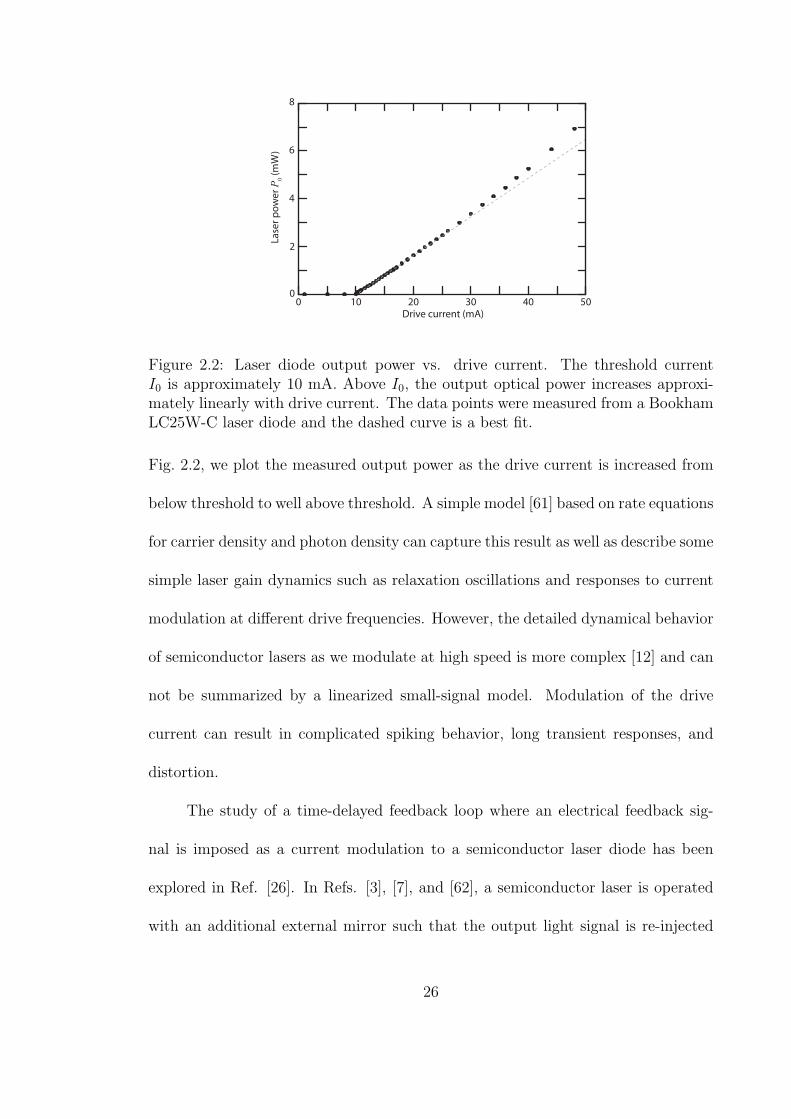
Figure 2.2: Laser diode output power vs. drive current. The threshold currentI0 is approximately 10 mA. Above I0, the output optical power increases approxi-mately linearly with drive current. The data points were measured from a BookhamLC25W-C laser diode and the dashed curve is a best fit.

Fig. 2.2, we plot the measured output power as the drive current is increased from

below threshold to well above threshold. A simple model [61] based on rate equations

for carrier density and photon density can capture this result as well as describe some

simple laser gain dynamics such as relaxation oscillations and responses to current

modulation at different drive frequencies. However, the detailed dynamical behavior

of semiconductor lasers as we modulate at high speed is more complex [12] and can

not be summarized by a linearized small-signal model. Modulation of the drive

current can result in complicated spiking behavior, long transient responses, and

distortion.

The study of a time-delayed feedback loop where an electrical feedback sig-

nal is imposed as a current modulation to a semiconductor laser diode has been

explored in Ref. [26]. In Refs. [3], [7], and [62], a semiconductor laser is operated

with an additional external mirror such that the output light signal is re-injected

26

into the laser cavity. The optical output is an irregular signal that reveals an intri-

cate interaction between chaotic dynamics and amplification of microscopic random

noise [63]. There is no complete analytic model that can show good quantitative

agreement with experimental measurement, making it difficult to fully diagnose the

observed behavior. In the series of experiments presented in this thesis, we oper-

ate the laser diode at a steady state point with output power P0, and we ignore

dynamical features and optical noise in our numerical models.

2.3 Single-mode optical fiber

Fiber optics are used to transmit data over long distances with low losses,

little distortion, and high speed. Optical signals are insensitive to RF interference

and mechanical vibration. The cables are lightweight, flexible, and inexpensive. For

these reasons, fiber optics is the standard for global communication, with a single

strand of optical fiber able to transmit several terabits of information per second

over a distance of many kilometers [21].

A fiber optic cable is a thin glass rod surrounded by a plastic protective buffer.

The glass is composed of an inner portion called the core and an outer portion called

the cladding. The core and cladding have different refractive indices such that a light

beam injected into the core will be guided along due to total internal reflection.

Snell’s law for refraction describes how light bends at an interface between two

dissimilar transmission media and is used to calculate the critical angle above which

refraction is impossible. In optical fiber, a light ray is incident on the cladding at

27

an angle greater than the critical angle of about 7 degrees, so the ray is completely

reflected and remains within the core. Historically, John Tyndall was one of the

first to demonstrate the principle of guided light via total internal reflection within

a narrow stream of flowing water at the Royal Institution Christmas Lecture in 1861

[64].

Single-mode fiber (SMF) allows for transmission of light along only a single

path. Multi-mode fiber, on the other hand, allows for numerous signals of the same

optical frequency to be sent over a single fiber. The number of allowed modes

is a function of the diameter of the code and cladding, with a larger diameter

supporting more modes of operation. SMF has a core diameter of 8–12 µm, a

cladding diameter of 125 µm, and a coating diameter of 250 µm. SMF has high

performance with respect to bandwidth and attenuation, principally because it is

completely insensitive to modal dispersion. SMF can transmit more than 40 Gb/s

over a single optical channel, and by using wavelength division multiplexing – in

which multiple signals are injected at slightly different optical wavelengths – one

SMF cable can transmit at data rates greater than 1 Tb/s. At 1550 nm, where losses

due to Rayleigh scattering, IR absorption, and molecular resonances are minimized,

a signal is attenuated by less than 0.2 dB per kilometer. At high optical power

levels, nonlinear effects in optical fiber can cause undesirable effects such as self

phase modulation, stimulated Raman scattering, and stimulated Brillouin scattering

[65]. In the experiments described in this thesis, the optical power is low and the

lengths of optical fiber is short enough as to ignore these effects.

SMF exhibits some degree of birefringence, meaning that it has a non-isotropic,

28

polarization-dependent refractive index. The birefringence properties are unpre-

dictable and vary along a length of fiber due changes in mechanical stresses such

as bends, temperature gradients, and irregularities in the shape of the core. Much

of telecommunications is insensitive to polarization, so SMF is appropriate. How-

ever, optical intensity modulators require a polarized input, so the signal between

a source laser and a modulator is often carried over polarization-maintaining fiber

(PMF). PMF has stress rods embedded within its fiber cladding which break the

circular symmetry of the core. Thus, two distinct polarization axes are maintained

throughout the waveguide.

2.4 Fiber polarization controller

A polarization controller is installed between the source laser and modulator,

since the modulator required a polarized input. A polarization controller transforms

an arbitrary input polarization state into an arbitrary output polarization state.

A fiber polarization controller is a simple and novel invention that exploits

the birefringence of SMF [66]. A birefringent crystal (such as fused silica in fiber

optics) has two optical axes along which light components travel at different speeds.

Birefringence, also called double refraction, is observed when an ordinary axis (or

slow axis) has a different refractive index from that of an extraordinary axis (or fast

axis). An injected light wave is resolved into these two axes, and, at the output,

there is a phase difference between the components, and thus a modified state of

polarization from that of the original beam. In a fiber polarization controller, SMF

29

is looped into three independent spools with relatively tight radii. The looping of

the fiber causes stress and induces birefringence. By twisting the paddle onto which

the fiber is looped, the principal axes of the SMF are rotated with respect to an

injected polarization vector. We emphasize that the birefringence is due to stress of

the loop and not the twisting of the paddles. Each loop follows the same principles

as those of a fractional wave plate (also called a retarder) in classical optics [67].

Hence a loop is called a fiber retarder. Three loops allow for complete control of a

polarization state. In terms of classical optics, first a quarter-wave plate transforms

the input to a linear polarization, next a half-wave plate rotates the linear state,

and finally another quarter-wave plate transforms to an arbitrary polarization.

A given rotation on a polarization controller paddle performs an unpredictable

retardance. In practice, the output intensity of the optical modulator is observed

and the three paddles are iteratively adjusted to maximize the throughput at the

beginning of an experiment.

2.5 Mach-Zehnder intensity modulator

As described in §2.1, an integrated Mach-Zehnder modulator is an interfero-

metric device whose optical transmission Pout/Pin is a function of an applied voltage

V . The electrooptic material used to form a relative phase shift within the two arms

of the interferometer is lithium niobate, which has a large electrooptic coefficient

r33 and is transparent over the optical communication spectrum. At the input, the

incident beam is polarized to orient the oscillating field along with extraordinary

30

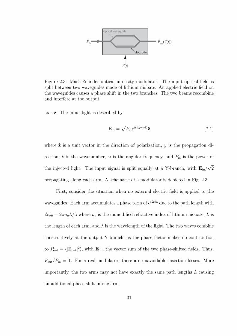
V(t)

Pin

Pout(V(t))

optical waveguide

electrode

Figure 2.3: Mach-Zehnder optical intensity modulator. The input optical field issplit between two waveguides made of lithium niobate. An applied electric field onthe waveguides causes a phase shift in the two branches. The two beams recombineand interfere at the output.

axis z. The input light is described by

Ein =√Pine

i(ky−ωt)z (2.1)

where z is a unit vector in the direction of polarization, y is the propagation di-

rection, k is the wavenumber, ω is the angular frequency, and Pin is the power of

the injected light. The input signal is split equally at a Y-branch, with Ein/√2

propagating along each arm. A schematic of a modulator is depicted in Fig. 2.3.

First, consider the situation when no external electric field is applied to the

waveguides. Each arm accumulates a phase term of ei∆ϕ0 due to the path length with

∆ϕ0 = 2πneL/λ where ne is the unmodified refractive index of lithium niobate, L is

the length of each arm, and λ is the wavelength of the light. The two waves combine

constructively at the output Y-branch, as the phase factor makes no contribution

to Pout = ⟨|Eout|2⟩, with Eout the vector sum of the two phase-shifted fields. Thus,

Pout/Pin = 1. For a real modulator, there are unavoidable insertion losses. More

importantly, the two arms may not have exactly the same path lengths L causing

an additional phase shift in one arm.

31

Now consider the case when a dc electric field of strength Ez is applied across

the two arms of the interferometer. The field is applied to each arm in an opposite

direction, i.e. it is applied in the +z direction for one arm and in the −z direction for

the other. Lithium niobate experiences a shift in its refractive index ne → ne+∆ne

given by

∆ne = 2πn3er33Ez

L

λ(2.2)

where r33 is electrooptic coefficient, Ez = V/d is the dc field, V is the applied

voltage, and d is the distance between electrodes supplying the field. In one arm,

the phase will see an additional phase of ∆ϕ = 2π∆neL/λ and the other arm will

see the opposite phase shift −∆ϕ. The combined optical power is

Pout(V ) =Pin

4⟨|e+i∆ϕ + e−i∆ϕ|2⟩ (2.3)

= Pin cos2

[πV

2Vπ

](2.4)

where we have defined the halfwave voltage

Vπ ≡ dλ

2n3er33L

. (2.5)

For lithium niobate ne = 2.2 and r33 = 30 pm/V. For a typical modulator, L = 5

cm and d = 100 µm. Optical communications often uses λ = 1550 nm, as described

in §2.3. With these values, Vπ = 4.85 V. For commercially available modulators, Vπ

is typically between 3 and 6 volts.

Eq. (2.4) implies that at V = 0 (no applied voltage), Pout = Pin. A more

realistic model for the Mach-Zehnder intensity modulator transfer function is

Pout(V ) = ηPin cos2

[πV

2Vπ

+ ϕ0

](2.6)

32

RF input voltage VO

pti

cal t

ran

smis

sio

n

0

0

0.2

0.4

0.6

0.8

1.0

−15 −10 −5 5 10 15

measuredtheory

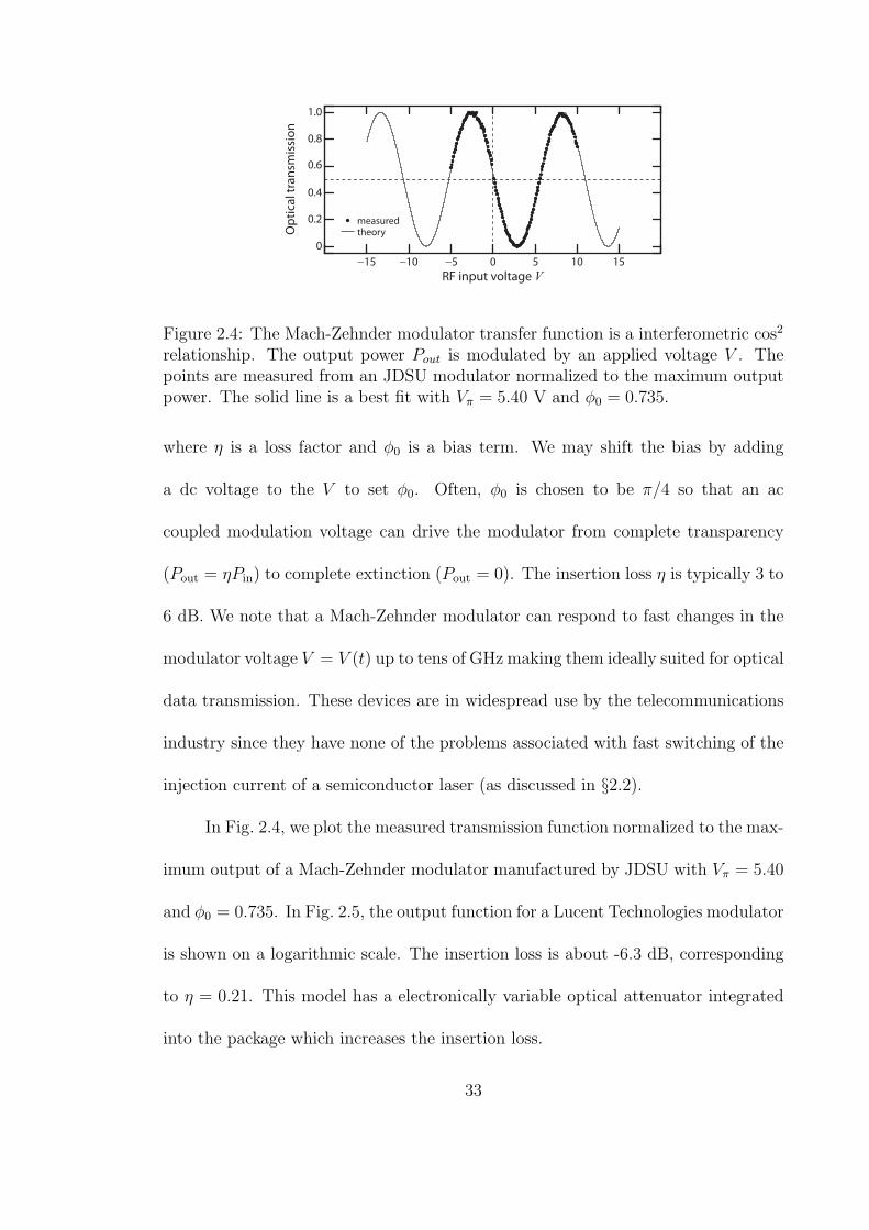
Figure 2.4: The Mach-Zehnder modulator transfer function is a interferometric cos2

relationship. The output power Pout is modulated by an applied voltage V . Thepoints are measured from an JDSU modulator normalized to the maximum outputpower. The solid line is a best fit with Vπ = 5.40 V and ϕ0 = 0.735.

where η is a loss factor and ϕ0 is a bias term. We may shift the bias by adding

a dc voltage to the V to set ϕ0. Often, ϕ0 is chosen to be π/4 so that an ac

coupled modulation voltage can drive the modulator from complete transparency

(Pout = ηPin) to complete extinction (Pout = 0). The insertion loss η is typically 3 to

6 dB. We note that a Mach-Zehnder modulator can respond to fast changes in the

modulator voltage V = V (t) up to tens of GHz making them ideally suited for optical

data transmission. These devices are in widespread use by the telecommunications

industry since they have none of the problems associated with fast switching of the

injection current of a semiconductor laser (as discussed in §2.2).

In Fig. 2.4, we plot the measured transmission function normalized to the max-

imum output of a Mach-Zehnder modulator manufactured by JDSU with Vπ = 5.40

and ϕ0 = 0.735. In Fig. 2.5, the output function for a Lucent Technologies modulator

is shown on a logarithmic scale. The insertion loss is about -6.3 dB, corresponding

to η = 0.21. This model has a electronically variable optical attenuator integrated

into the package which increases the insertion loss.

33

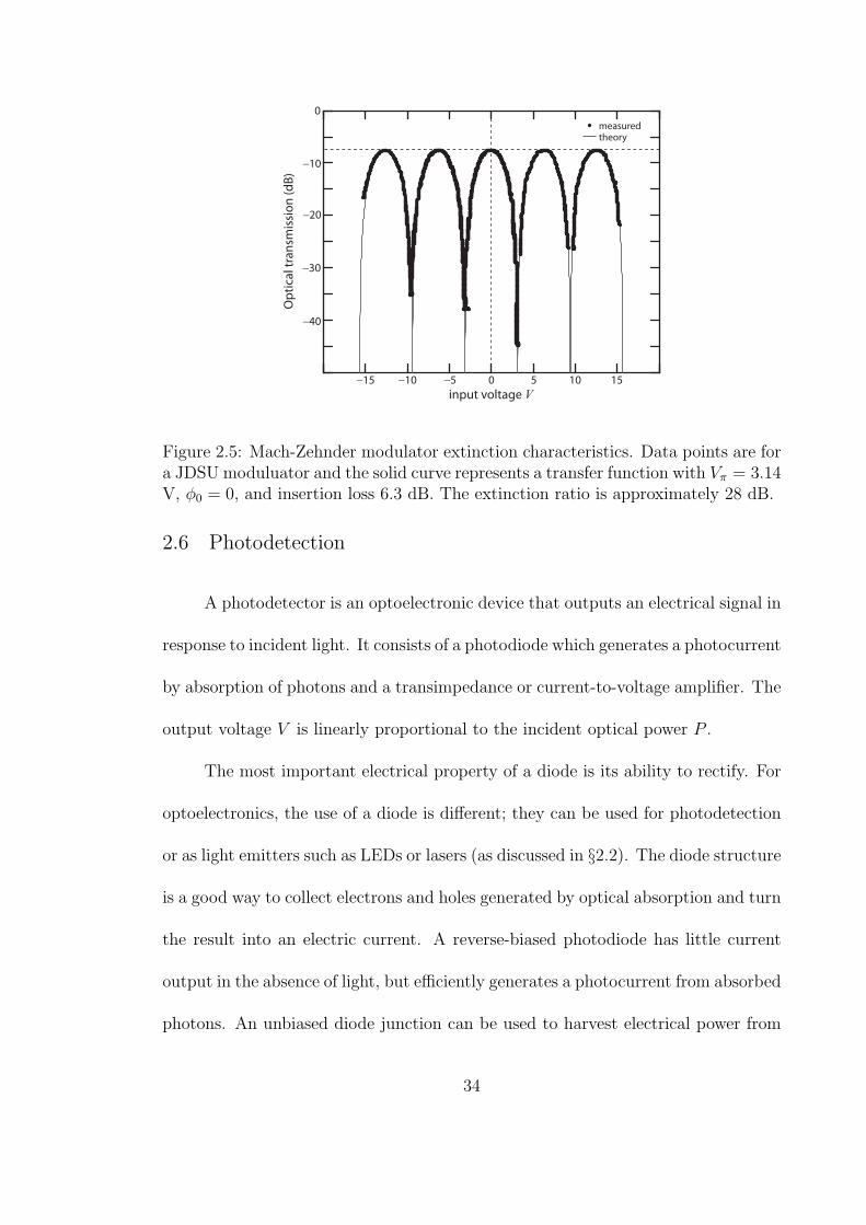
measuredtheory

input voltage V

Op

tica

l tra

nsm

issi

on

(d

B)

0−15

−40

−30

−20

−10

0

−10 −5 5 10 15

Figure 2.5: Mach-Zehnder modulator extinction characteristics. Data points are fora JDSU moduluator and the solid curve represents a transfer function with Vπ = 3.14V, ϕ0 = 0, and insertion loss 6.3 dB. The extinction ratio is approximately 28 dB.

2.6 Photodetection

A photodetector is an optoelectronic device that outputs an electrical signal in

response to incident light. It consists of a photodiode which generates a photocurrent

by absorption of photons and a transimpedance or current-to-voltage amplifier. The

output voltage V is linearly proportional to the incident optical power P .

The most important electrical property of a diode is its ability to rectify. For

optoelectronics, the use of a diode is different; they can be used for photodetection

or as light emitters such as LEDs or lasers (as discussed in §2.2). The diode structure

is a good way to collect electrons and holes generated by optical absorption and turn

the result into an electric current. A reverse-biased photodiode has little current

output in the absence of light, but efficiently generates a photocurrent from absorbed

photons. An unbiased diode junction can be used to harvest electrical power from

34

light, as in a solar cell [68].

A photodiode is characterized by its quantum efficiency ηq (defined as the num-

ber of electrons produced per incident photon) and responsivity S (the photocurrent

per unit incident optical power). A well-designed photodiode absorbs essentially all

the incident photons and thus achieve close to ηq = 1. The responsivity, measured

in units of A/W, is given as

S =ηqq

~ω(2.7)

where q is the charge of an electron and ~ω is the quanta of energy delivered by a

single photon. The fiber-coupled InGaAS photodiodes used in this set of experiments

have a responsivity of 0.9 A/W at 1550 nm. Typically, the transimpedance gainGTIA

is on the order of 1000 V/A. Thus a P = 0.2 mW optical signal will produce a dc

voltage of V = GTIASP = 180 mV. However, the high-gain amplifier is ac-coupled,

so it only passes fluctuating signals as an output voltage. For telecommunications-

grade drives, the pass band typically goes from tens of kHz to many GHz.

2.7 Electronic amplification

The ac-coupled output voltage of the photodetector has an amplitude in the

range of 10s of millivolts. The characteristic voltage for an optical modulator is

Vπ ∼ 5 V. A voltage gain Gamp is required to boost the feedback signal to an

appropriate level in order to observe interesting dynamics. A high-gain, broadband

RF amplifier is employed. The MiniCircuits TIA-1000-1R8 has a rated gain of 38

dB within the band of 500 kHz to 1 GHz and provides sufficient power to drive the

35

0

Frequency (GHz)

(a)

(b)

Fee

db

ack

ga

in (

dB

)

0.5 1.0 1.5 2.0

+40

0

−40

−80

0

Frequency (GHz)

Fee

db

ack

ga

in

0.5 1.0 1.5 2.0

20

15

10

5

0

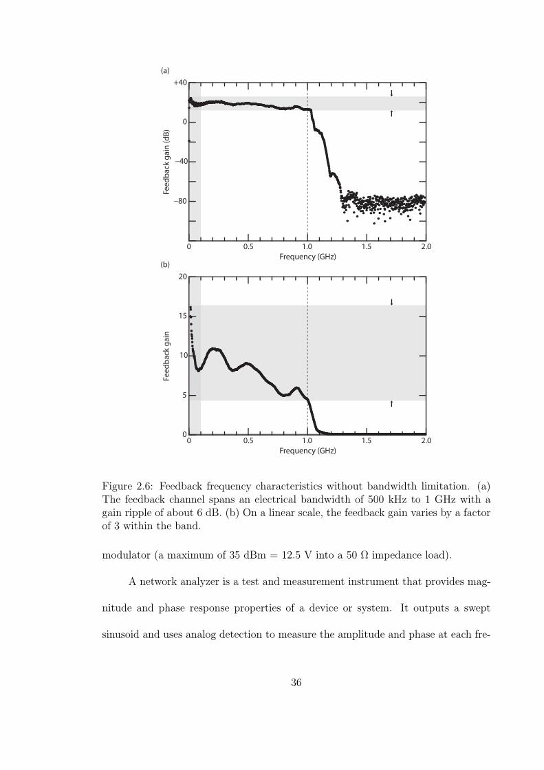
Figure 2.6: Feedback frequency characteristics without bandwidth limitation. (a)The feedback channel spans an electrical bandwidth of 500 kHz to 1 GHz with again ripple of about 6 dB. (b) On a linear scale, the feedback gain varies by a factorof 3 within the band.

modulator (a maximum of 35 dBm = 12.5 V into a 50 Ω impedance load).

A network analyzer is a test and measurement instrument that provides mag-

nitude and phase response properties of a device or system. It outputs a swept

sinusoid and uses analog detection to measure the amplitude and phase at each fre-

36

quency. The network analyzer test signal is injected as the modulator voltage and

the amplifier output measured. In Fig. 2.6, the magnitude response is plotted for an

open loop. For this measurement, a New Focus 1611 photodectector and a MiniCir-

cuits power amplifier were used in the optoelectronic feedback path. The highpass

cut-on frequencies are 30 kHz and 500 kHz respectively, and each has a lowpass

cutoff frequency of 1 GHz. In (a), the magnitude is plotted on a semilogarithmic

scale. As expected, the gain is relatively flat over the pass band and is strongly

attenuated below and above it. In the pass band, there is a gain ripple of 3–6 dB,

which is typical for a broadband, high-gain amplifier. The same data is plotted on

a linear scale in (b). Here, we notice that a 3–6 dB gain ripple corresponds to large

linear variation. A low frequency signal is amplified almost twice as strongly as a

high frequency signal.

When the feedback loop is closed, interesting dynamical waveforms are ob-

served. However, it is difficult to construct an analytic model that matches the

observed behavior with sufficient accuracy for the studies presented in Chapters 4

and 5. The strong roll-off in feedback gain at low and high frequency can be modeled

as high-order linear filters, but realistically capturing the details of the gain ripple

within a model remains a challenge. Our solution is to modify the experimental sys-

tem by intentionally restricting the bandwidth to a range where the gain ripple is

small by incorporating a well-understood bandpass filter within the feedback path.

This is the subject of §2.8.

37

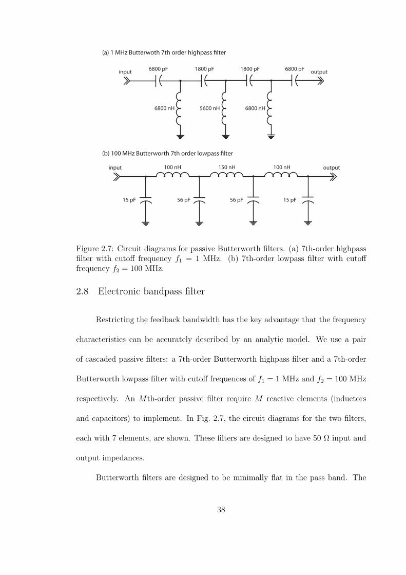
input

(a) 1 MHz Butterwoth 7th order highpass lter

6800 pF

6800 nH 5600 nH 6800 nH

1800 pF 1800 pF 6800 pFoutput

outputinput

(b) 100 MHz Butterworth 7th order lowpass lter

15 pF 56 pF 56 pF 15 pF

100 nH 150 nH 100 nH

Figure 2.7: Circuit diagrams for passive Butterworth filters. (a) 7th-order highpassfilter with cutoff frequency f1 = 1 MHz. (b) 7th-order lowpass filter with cutofffrequency f2 = 100 MHz.

2.8 Electronic bandpass filter

Restricting the feedback bandwidth has the key advantage that the frequency

characteristics can be accurately described by an analytic model. We use a pair

of cascaded passive filters: a 7th-order Butterworth highpass filter and a 7th-order

Butterworth lowpass filter with cutoff frequences of f1 = 1 MHz and f2 = 100 MHz

respectively. An Mth-order passive filter require M reactive elements (inductors

and capacitors) to implement. In Fig. 2.7, the circuit diagrams for the two filters,

each with 7 elements, are shown. These filters are designed to have 50 Ω input and

output impedances.

Butterworth filters are designed to be minimally flat in the pass band. The

38

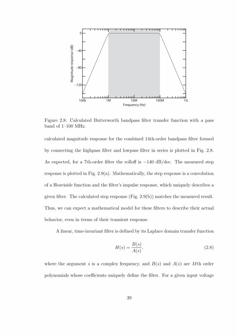
100k

0

−40

−80

−120

Frequency (Hz)

Ma

gn

itu

de

re

spo

nse

(d

B)

1M 10M 100M 1G

Figure 2.8: Calculated Butterworth bandpass filter transfer function with a passband of 1–100 MHz.

calculated magnitude response for the combined 14th-order bandpass filter formed

by connecting the highpass filter and lowpass filter in series is plotted in Fig. 2.8.

As expected, for a 7th-order filter the rolloff is −140 dB/dec. The measured step

response is plotted in Fig. 2.9(a). Mathematically, the step response is a convolution

of a Heaviside function and the filter’s impulse response, which uniquely describes a

given filter. The calculated step response (Fig. 2.9(b)) matches the measured result.

Thus, we can expect a mathematical model for these filters to describe their actual

behavior, even in terms of their transient response.

A linear, time-invariant filter is defined by its Laplace domain transfer function

H(s) =B(s)

A(s), (2.8)

where the argument s is a complex frequency, and B(s) and A(s) are Mth order

polynomials whose coefficients uniquely define the filter. For a given input voltage

39

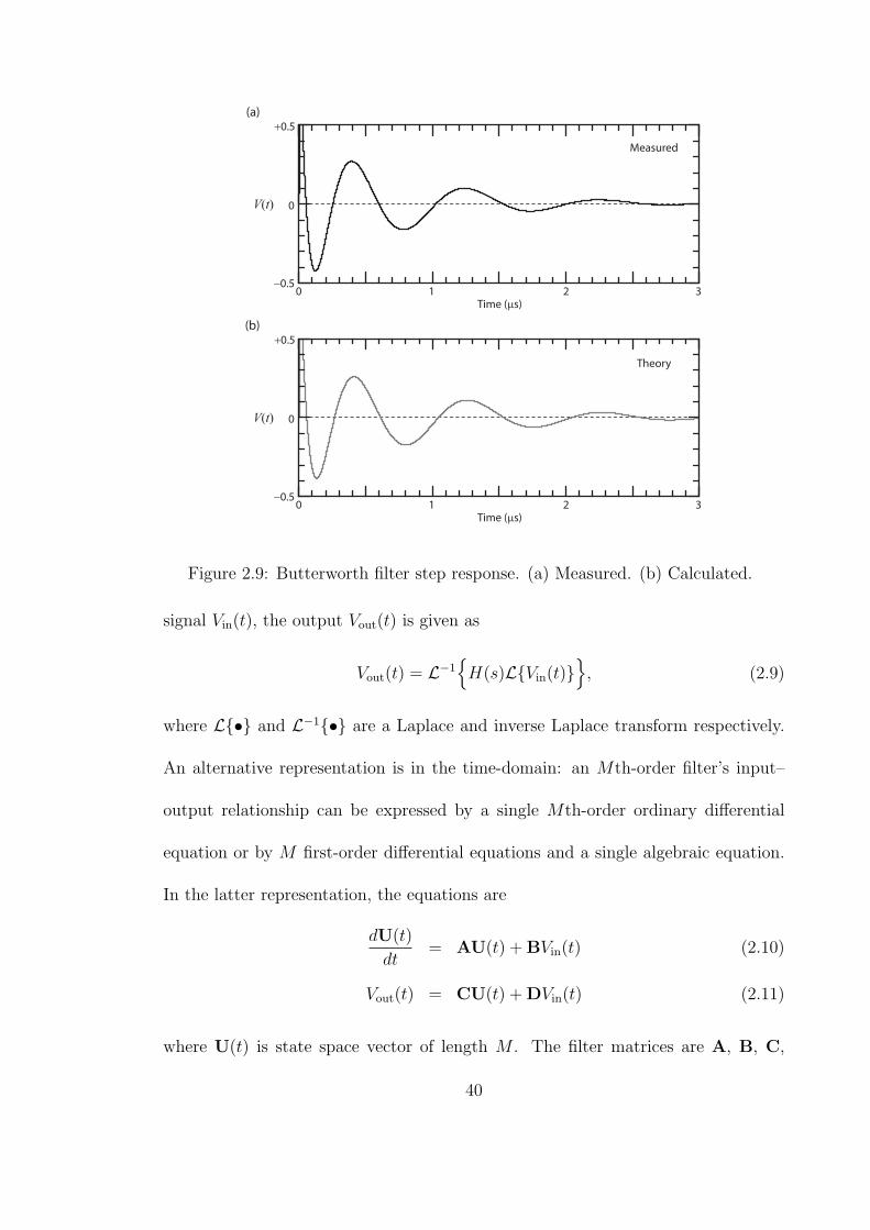
0

0

+0.5

−0.51

Time (µs)

Measured

Theory

V(t)

2 3

(a)

0

0

+0.5

−0.51

Time (µs)

V(t)

2 3

(b)

Figure 2.9: Butterworth filter step response. (a) Measured. (b) Calculated.

signal Vin(t), the output Vout(t) is given as

Vout(t) = L−1H(s)LVin(t)

, (2.9)

where L• and L−1• are a Laplace and inverse Laplace transform respectively.

An alternative representation is in the time-domain: an Mth-order filter’s input–

output relationship can be expressed by a single Mth-order ordinary differential

equation or by M first-order differential equations and a single algebraic equation.

In the latter representation, the equations are

dU(t)

dt= AU(t) +BVin(t) (2.10)

Vout(t) = CU(t) +DVin(t) (2.11)

where U(t) is state space vector of length M . The filter matrices are A, B, C,

40

and D which can be derived from the coefficients of A(s) and B(s). For the 14th-

order bandpass filter described above, A is (14 × 14), B is (14 × 1), C is (1 × 14),

and D is (1× 1). For a strictly proper transfer function (for which the polynomial

order of B(s) is greater than the order of A(s)), D = 0. The matrices for a given

polynomial transfer function H(s) can be directly computed using Matlab. For a

filter with M ≥ 2, there are many different state state realizations for the same

transfer function H(s), and, in practice, some representations may be numerically

unstable.

2.9 Time delay

Time delay is due to the length of optical fiber between the modulator and

detector and lengths of the RF cables between the individual components. The

refractive index of SMF is nSMF = 1.47, so the light signal propagates at v = c/n =

0.204 m/ns. For copper coaxial cable with a solid dielectric, ncoax ≈ 1.52 so the

signals travels at v = 0.198 m/ns. For the experiments described in Chapters 3 and

4, the total measured round-trip time delay τ is 22.45 ns, corresponding to a total

length of fiber and RF cable of about 5.5 m.

A method to have much longer time delays (applied in the experiments de-

scribed in Chapters 6 and 7) without requiring an impractical bundle of cables is

to use a combination of an analog-to-digital convertor (ADC), a bank of digital

shift registers, and a digital-to-analog converter (DAC). A digital signal processing

(DSP) board (Spectrum Digital DSK6713), originally designed for audio processing,

41

V(t)

MZM

Laser

diode Photoreceiver

AmplierDigital signal

processor board

ADCDACDSP

RAM

Figure 2.10: Schematic of an optoelectronic feedback loop using a DSP board fordelay and filtering.

packages all these components along with a programmable microprocessor. Signal

delays of milliseconds to minutes are possible by continuously storing the sampled

signal in a memory buffer for a programmed number of sample intervals.

The ADC and DAC are capable of recording and transmitting analog signals

at up to 48 kHz when the sample rate is set to 96 kilosamples/s. To use a DSP

board for delay, one must modify the frequency characteristics of the rest of the

feedback loop to operate at audio speeds. Principally, the transimpedance and

voltage amplifiers must respond to low frequency inputs. This is achieved using

operational amplifier (LM741) circuits for both. The analog filter (described in

§2.8) is replaced with a digital filter programmed on the DSP, with a pass band

from a few Hz up to tens of kHz. Fig. 4.13 is a schematic of a DSP-based feedback

loop. The details for the DSP-based optoelectronic feedback loop are presented in

Refs. [8], [42], and [69]. We note that scaling down the frequencies into the audio

range and using a DSP board within the feedback architecture greatly increases

flexibility and controllability. More importantly, the system uses only low-cost and

42

widely-available components, making this an ideal system for experiments involving

numerous realizations of identical systems. Using a high performance DSP system

or a mixed-signal field-programmable gate array, the same feedback operations could

be performed at hundreds of megahertz.

2.10 Continuous-time delay differential equation model

In this section, we merge the mathematical descriptions of the individual com-

ponents that form a complete optoelectronic feedback loop into a single delay dif-

ferential equation model. Here, we consider a loop with analog filters described in

§2.8. This model captures all the salient features of the dynamics by incorporat-

ing the nonlinearity, time delay, and bandwidth limitation. It provides very good

quantitative agreement with the experimental observations, as will be presented in

Chapter 3. However, we emphasize that this simple model is imperfect and neglects

effects which may be essential in some circumstances. The model does not include

electronic and optical noise terms, hysteresis due to time-varying parameters, or

feedback gain ripple.

Since the system is a loop, the dynamics may be modeled at any point in

the loop. It suffices to consider variables representing the output voltage of the

electronic filter Vout and the state space vector of the filter U to determine the

solution everywhere in the loop. Tracing along the experimental schematic (Fig. 2.1),

the output of the filter is amplified by a gain Gamp. The voltage V (t) = GampVout(t)

is applied to the modulator as the modulation voltage. We note that, in reality, the

43

delay is distributed throughout the loop, but for modeling purposes it is adequate to

assume an instantaneous transfer between components and one single lumped delay

τ . The optical power is modulated by the drive voltage with a response given by

Eq. (2.5):

P (t) = ηP0 cos2

[πGampVout(t)

2Vπ

+ ϕ0

], (2.12)

where P0 is the steady optical power injected into the modulator. Next, this optical

signal is incident on the photodetector with a linear responsivity S and gain GTIA.

In the real situation, the photodetector output voltage is highpass filtered. Since

the dominant source of bandwidth restriction is the 14th-order Butterworth filters

which have cutoff frequencies well above and below every other component, it is

reasonable to disregard all other filtering operations (at the photodetector and RF

amplifier). A dc-coupled version of the photodetector output voltage is:

VPD(t) = GTIASηP0 cos2

[πGampVout(t)

2Vπ

+ ϕ0

]. (2.13)

This is precisely the input signal to the filter, after it has been delayed by τ . The

complete feedback loop model is thus:

dU(t)

dt= AU(t) +BGTIASηP0 cos

2

[πGampVout(t− τ)

2Vπ

+ ϕ0

](2.14)

Vout(t) = CU(t) (2.15)

where we have used the fact that D = 0 for the bandpass filter. Inserting Eq. (2.14)

into (2.13), we have

dU(t)

dt= AU(t) +BGTIASηP0 cos

2

[πGampCU(t− τ)

2Vπ

+ ϕ0

]. (2.16)

44

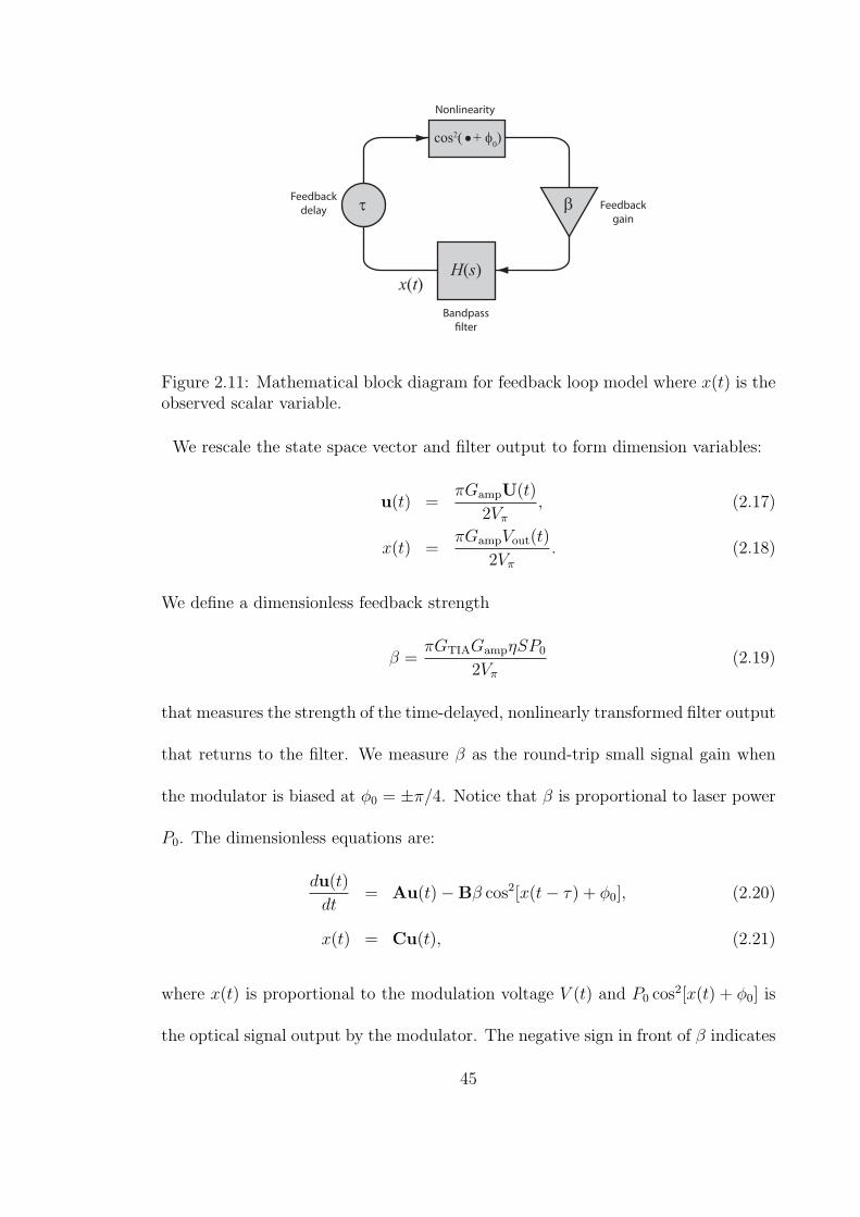
Nonlinearity

Feedback

gain

Bandpass

lter

Feedback

delay

cos2( + φ0)

βτ

H(s)x(t)

Figure 2.11: Mathematical block diagram for feedback loop model where x(t) is theobserved scalar variable.

We rescale the state space vector and filter output to form dimension variables:

u(t) =πGampU(t)

2Vπ

, (2.17)

x(t) =πGampVout(t)

2Vπ

. (2.18)

We define a dimensionless feedback strength

β =πGTIAGampηSP0

2Vπ

(2.19)

that measures the strength of the time-delayed, nonlinearly transformed filter output

that returns to the filter. We measure β as the round-trip small signal gain when

the modulator is biased at ϕ0 = ±π/4. Notice that β is proportional to laser power

P0. The dimensionless equations are:

du(t)

dt= Au(t)−Bβ cos2[x(t− τ) + ϕ0], (2.20)

x(t) = Cu(t), (2.21)

where x(t) is proportional to the modulation voltage V (t) and P0 cos2[x(t) + ϕ0] is

the optical signal output by the modulator. The negative sign in front of β indicates

45

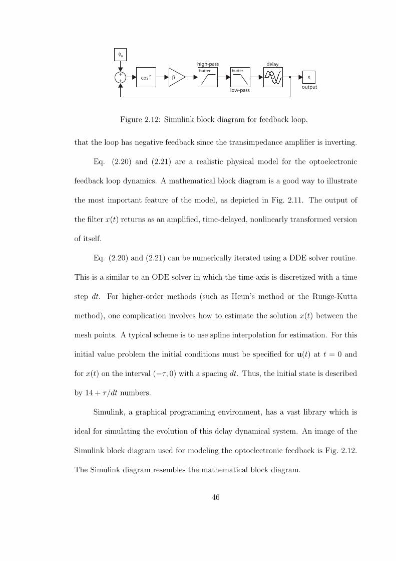
cos 2 β

φ0

butter butter

x+

+

delay

output

high-pass

low-pass

Figure 2.12: Simulink block diagram for feedback loop.

that the loop has negative feedback since the transimpedance amplifier is inverting.

Eq. (2.20) and (2.21) are a realistic physical model for the optoelectronic

feedback loop dynamics. A mathematical block diagram is a good way to illustrate

the most important feature of the model, as depicted in Fig. 2.11. The output of

the filter x(t) returns as an amplified, time-delayed, nonlinearly transformed version

of itself.

Eq. (2.20) and (2.21) can be numerically iterated using a DDE solver routine.

This is a similar to an ODE solver in which the time axis is discretized with a time

step dt. For higher-order methods (such as Heun’s method or the Runge-Kutta

method), one complication involves how to estimate the solution x(t) between the

mesh points. A typical scheme is to use spline interpolation for estimation. For this

initial value problem the initial conditions must be specified for u(t) at t = 0 and

for x(t) on the interval (−τ, 0) with a spacing dt. Thus, the initial state is described

by 14 + τ/dt numbers.

Simulink, a graphical programming environment, has a vast library which is

ideal for simulating the evolution of this delay dynamical system. An image of the

Simulink block diagram used for modeling the optoelectronic feedback is Fig. 2.12.

The Simulink diagram resembles the mathematical block diagram.

46

2.11 Discrete-time map equation model

When a DSP board is used to implement the feedback delay and filter oper-

ations, the physical model is similar to that of the continuous-time case. In fact,

one can effectively use the same model by appropriately selecting the set of ma-

trices A,B,C,D for the particular digital filter realization and scaling the delay

τ . However, under some circumstances an accurate representation requires trans-

forming the analog filter to a digital filter operating in discrete time. We note that

this transformation must be undertaken in order to program the DSP, and thus a

discrete time model is actually an exact description of the filter. Instead of consid-

ering the variable x(t) whose domain is all of time t, the discrete time solution is

given only at the sample times nTs = n/fs where Ts is the time interval between

successive samples of the ADC, fs is the sampling rate, and n is an integer. The

time-series x[n] is given by a map equation with the iterate x[n + 1] a function of

the past iterates: x[n], x[n− 1], . . ..

The design of a digital filter that mimics an analog filter is presented in Refs.

[8], [42], and [69]. The basic transformation takes the Laplace domain transfer func-

tion Ha(s) to its z-domain counterpart Hd(z). A major distinction between these

representations is that a digital filter has a strict upper bound for the bandwidth

given as the Nyquist rate fN = fs/2, and for an analog filter, frequencies can go off to

infinity. If the desired lowpass cutoff frequency f2 is well below fN, then this aspect

has minimal consequences, and hence the continuous-time equations are valid.

The discrete-time equations of motion can be motivated by drawing a mathe-

47

Nonlinearity

Feedback

gain

Digital lter

Feedback

delay

cos2( + φ0)

β

H(z)x[n]

x[n−1]

x[n−2]

x[n−k]

Figure 2.13: Mathematical block diagram for discrete-time feedback loop model.

matical block diagram (Fig. 2.13). x[n] is the output of the filter at time n, and it

returns as the filter input as −β cos2(x[n− k] + ϕ0) where k = τ/Ts is the feedback

delay in terms of length of the memory buffer. A generic digital filter can be written

as:

xout[n] = −M∑

m=1

amxout[n−m] +M∑

m=0

bmxin[n−m] (2.22)

where M is the order of the filter and the 2M + 1 coefficients am, bm are specific

to the filter design. For the simplest bandpass filter (M = 2) with fs = 24 kHz,

f1 = 100 Hz, and f2 = 2.5 kHz, the parameters are a1 = −1.4962, a2 = 0.5095, b0 =

−b2 = 0.2452, and b0 = 0. Thus the discrete-time dynamics of the optoelectronic

feedback loop are described by the map:

x[n] = −a1x[n−1]−a2x[n−2]−b0β(cos(x[n−k]+ϕ0)−cos(x[n−k−2]+ϕ0)). (2.23)

This map is an extremely simple and elegant formulation that encapsulates all the

salient features of the time-delay feedback loop dynamics. By iterating x while vary-

ing the parameter β, one can see a striking array of complex waveforms (presented

in Refs. [8] and [69]).

48

2.12 Summary

1. The modular components of an optoelectronic feedback loop are ubiquitous in

telecommunication networks and are thus widely available at low-cost.

2. The physics of each component is well understood and conducive to numerical

modeling.

3. By imposing a bandwidth restriction on the feedback path with an electronic

bandpass filter, we avoid modeling the complicated gain ripple behavior of the

RF amplifier.

4. The time scales of a feedback loop (bandwidth and time delay) can be modified

to operate anywhere from the audio to microwave range.

5. A digital signal processing board allows for real-time control and exact repli-

cation of system parameters.

49

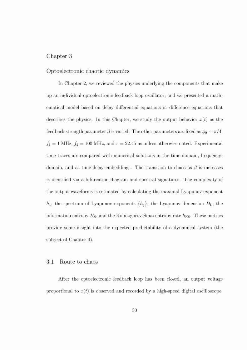
Chapter 3

Optoelectronic chaotic dynamics

In Chapter 2, we reviewed the physics underlying the components that make

up an individual optoelectronic feedback loop oscillator, and we presented a math-

ematical model based on delay differential equations or difference equations that

describes the physics. In this Chapter, we study the output behavior x(t) as the

feedback strength parameter β is varied. The other parameters are fixed as ϕ0 = π/4,

f1 = 1 MHz, f2 = 100 MHz, and τ = 22.45 ns unless otherwise noted. Experimental

time traces are compared with numerical solutions in the time-domain, frequency-

domain, and as time-delay embeddings. The transition to chaos as β is increases

is identified via a bifurcation diagram and spectral signatures. The complexity of

the output waveforms is estimated by calculating the maximal Lyapunov exponent

h1, the spectrum of Lyapunov exponents hj, the Lyapunov dimension DL, the

information entropy HS, and the Kolmogorov-Sinai entropy rate hKS. These metrics

provide some insight into the expected predictability of a dynamical system (the

subject of Chapter 4).

3.1 Route to chaos

After the optoelectronic feedback loop has been closed, an output voltage

proportional to x(t) is observed and recorded by a high-speed digital oscilloscope.

50

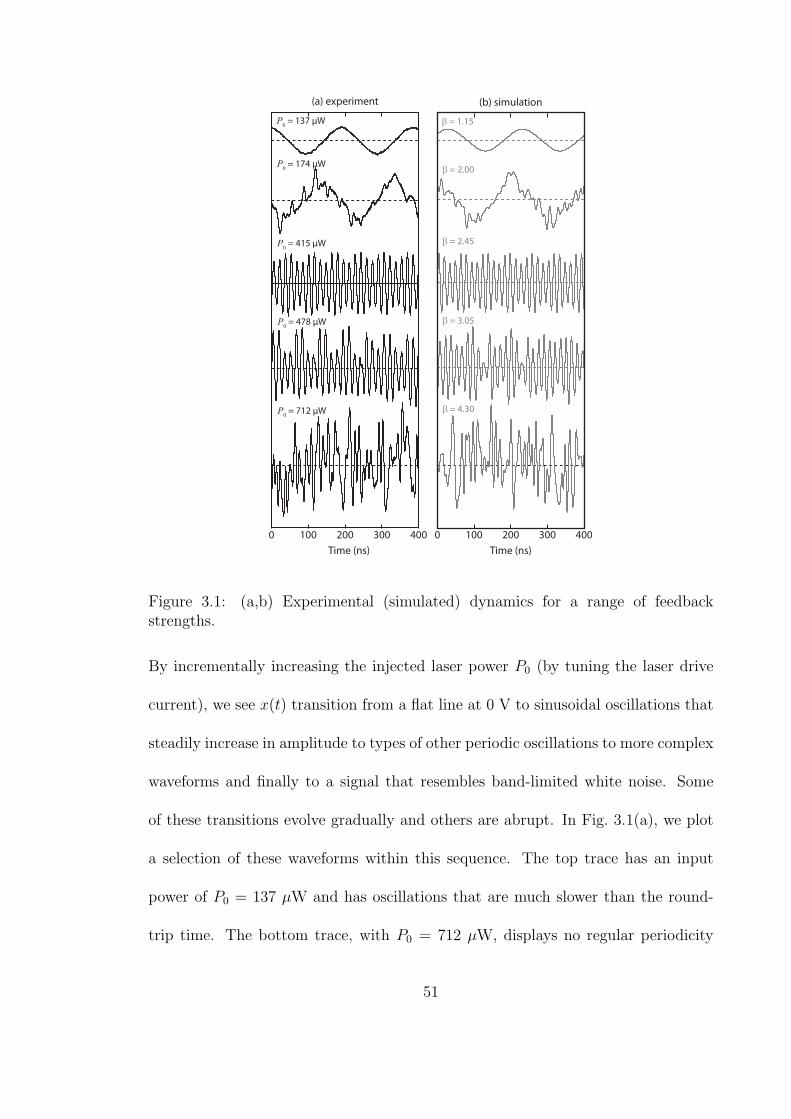
0 100 200

Time (ns)

300 400 0 100 200

Time (ns)

300 400

P0 = 137 µW

P0 = 174 µW

P0 = 415 µW

P0 = 478 µW

P0 = 712 µW

β = 1.15

β = 2.00

β = 2.45

β = 3.05

β = 4.30

(a) experiment (b) simulation

Figure 3.1: (a,b) Experimental (simulated) dynamics for a range of feedbackstrengths.

By incrementally increasing the injected laser power P0 (by tuning the laser drive

current), we see x(t) transition from a flat line at 0 V to sinusoidal oscillations that

steadily increase in amplitude to types of other periodic oscillations to more complex

waveforms and finally to a signal that resembles band-limited white noise. Some

of these transitions evolve gradually and others are abrupt. In Fig. 3.1(a), we plot

a selection of these waveforms within this sequence. The top trace has an input

power of P0 = 137 µW and has oscillations that are much slower than the round-

trip time. The bottom trace, with P0 = 712 µW, displays no regular periodicity

51

Laser power P0 (µW)

100 200 300 400 500 600 700 800 900

x

β

1.0 2.0 3.0 4.01.5 2.5 3.5 4.5 5.0−4

−2

0

2

4

x

−4

−2

0

2

4

(a) experiment

(b) simulation

Figure 3.2: Bifurcation diagrams as the feedback strength is increased. (a) Fromexperimental time traces for increasing laser power P0. (b) From numerical time-series as the parameter β is increases. The vertical lines point to time-series thathave matching behavior.

or apparent structure. Fig. 3.1(b) plots numerically integrated time-series (Eqs.

(2.20) and (2.21)) for a series of feedback strength β, where each simulation was

begun from random initial conditions and a long transient period was discarded.

Each experimental trace is seen to have a numerical partner that shares its basic

temporal features. We conclude that the model is adequate for representing the real

system’s behavior, and we may expect that analytical studies of the mathematical

model will have real physical consequences.

The route to chaos is summarized with a bifurcation diagram. A histogram

52

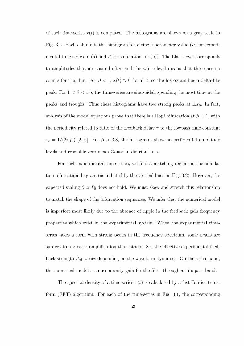
of each time-series x(t) is computed. The histograms are shown on a gray scale in

Fig. 3.2. Each column is the histogram for a single parameter value (P0 for experi-

mental time-series in (a) and β for simulations in (b)). The black level corresponds

to amplitudes that are visited often and the white level means that there are no

counts for that bin. For β < 1, x(t) ≈ 0 for all t, so the histogram has a delta-like

peak. For 1 < β < 1.6, the time-series are sinusoidal, spending the most time at the

peaks and troughs. Thus these histograms have two strong peaks at ±x0. In fact,

analysis of the model equations prove that there is a Hopf bifurcation at β = 1, with

the periodicity related to ratio of the feedback delay τ to the lowpass time constant

τ2 = 1/(2πf2) [2, 6]. For β > 3.8, the histograms show no preferential amplitude

levels and resemble zero-mean Gaussian distributions.

For each experimental time-series, we find a matching region on the simula-

tion bifurcation diagram (as indicted by the vertical lines on Fig. 3.2). However, the

expected scaling β ∝ P0 does not hold. We must skew and stretch this relationship

to match the shape of the bifurcation sequences. We infer that the numerical model

is imperfect most likely due to the absence of ripple in the feedback gain frequency

properties which exist in the experimental system. When the experimental time-

series takes a form with strong peaks in the frequency spectrum, some peaks are

subject to a greater amplification than others. So, the effective experimental feed-

back strength βeff varies depending on the waveform dynamics. On the other hand,

the numerical model assumes a unity gain for the filter throughout its pass band.

The spectral density of a time-series x(t) is calculated by a fast Fourier trans-

form (FFT) algorithm. For each of the time-series in Fig. 3.1, the corresponding

53

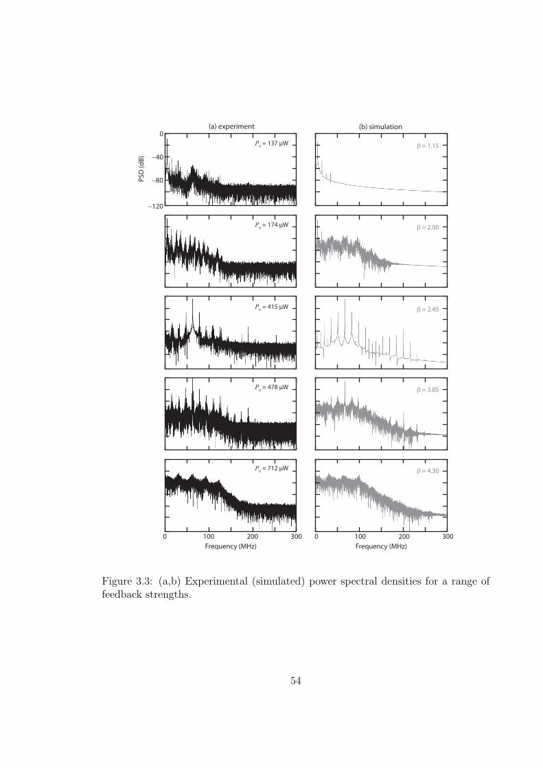
0

0

−40

−80

−120

100

Frequency (MHz)

PS

D (

dB

)

Frequency (MHz)

200 300 0 100 200 300

(a) experiment (b) simulation

P0 = 137 µW

P0 = 174 µW

P0 = 415 µW

P0 = 478 µW

P0 = 712 µW

β = 1.15

β = 2.00

β = 2.45

β = 3.05

β = 4.30

Figure 3.3: (a,b) Experimental (simulated) power spectral densities for a range offeedback strengths.

54

100kFrequency (Hz)

Po

we

r sp

ect

ral d

en

sity

(d

B)

1M 10M 100M 1G

0

−40

−80

−120

P0 = 712 µW

Figure 3.4: The PSD for P0 = 712 µW has features of band-limited noise.

power spectral density (PSD) is plotted in Fig. 3.3. Again, we see an equivalence be-

tween the experimental and simulated spectral features. At low feedback strength,

there are strong dominant peaks. As the feedback strength is increased, the noise

floor rises up and eventually fills the entire pass band of 1–100 MHz. This is a sig-

nature that is often observed in a transition from non-chaotic to chaotic dynamics.

In Fig. 3.4, the PSD for P0 = 712 µW is shown with a logarithmic frequency

axis. This spectrum resembles white noise within the bandpass filter band with only

a few dominant spectral modes. In Ref. [6], this property is systematically studied

for the case when the modulator is biased at ϕ0 = 0 and with an ultra-wide band

feedback channel spanning six orders of magnitude (10 kHz – 10 GHz). For this

case, it is analytically derived that there remain no linearly stable periodic modes

embedded within the dynamics.

55

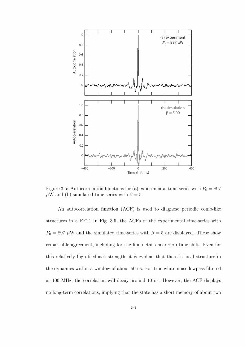
Au

toco

rre

lati

on

0

0.2

0.4

0.6

0.8

1.0

0

Time shift (ns)

(a) experiment

P0 = 897 µW

(b) simulation

β = 5.00

Au

toco

rre

lati

on

0

0.2

0.4

0.6

0.8

1.0

200 400−200−400

Figure 3.5: Autocorrelation functions for (a) experimental time-series with P0 = 897µW and (b) simulated time-series with β = 5.

An autocorrelation function (ACF) is used to diagnose periodic comb-like

structures in a FFT. In Fig. 3.5, the ACFs of the experimental time-series with

P0 = 897 µW and the simulated time-series with β = 5 are displayed. These show

remarkable agreement, including for the fine details near zero time-shift. Even for

this relatively high feedback strength, it is evident that there is local structure in

the dynamics within a window of about 50 ns. For true white noise lowpass filtered

at 100 MHz, the correlation will decay around 10 ns. However, the ACF displays

no long-term correlations, implying that the state has a short memory of about two

56

x(t)

x(t−Temb ) x(t−

2T emb)

1

1

0

00

−1−1

1

−1

x(t)

x(t−Temb ) x(t−

2T emb)

3

3

0

00

−3−3

3

−3

x(t)

x(t−Temb ) x(t−

2T emb)

3

3

0

00

−3

−3

3

−3

x(t)

x(t−τ) x(t−2Temb)

2

2

0

00

−2−2

2

−2

x(t)

x(t−Temb) x(t−2Temb

)

2

2

0

00

−2−2

2

−2

(a) P0 = 137 µW

(b) P0 = 415 µW

(c) P0 = 675 µW

x(t)

x(t−Temb ) x(t−

2T emb)

1

1

0

00

−1−1

1

−1

(d) β = 1.30

(e) β = 2.40

(f ) β = 3.90

Figure 3.6: Time-delay embedding for experimental and simulated time-series. (a,d)Temb = 20 ns, (b,e) Temb = 10 ns, (c,f) Temb = 1 ns.

57

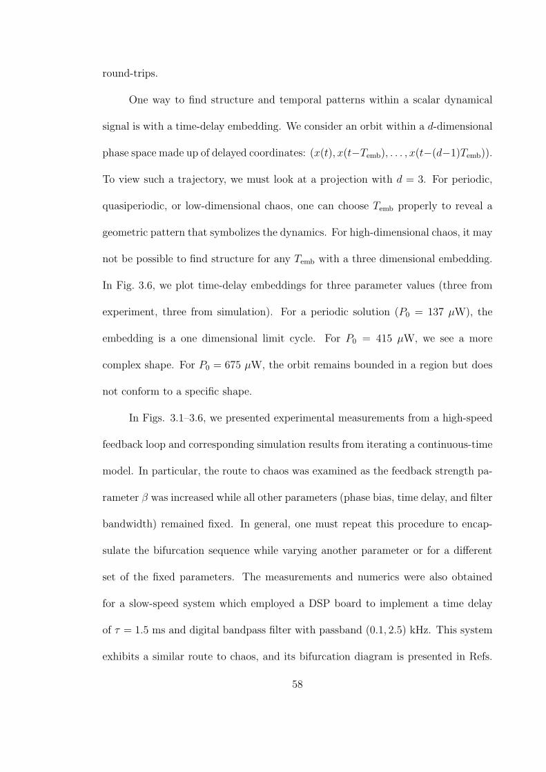
round-trips.

One way to find structure and temporal patterns within a scalar dynamical

signal is with a time-delay embedding. We consider an orbit within a d-dimensional

phase space made up of delayed coordinates: (x(t), x(t−Temb), . . . , x(t−(d−1)Temb)).

To view such a trajectory, we must look at a projection with d = 3. For periodic,

quasiperiodic, or low-dimensional chaos, one can choose Temb properly to reveal a

geometric pattern that symbolizes the dynamics. For high-dimensional chaos, it may

not be possible to find structure for any Temb with a three dimensional embedding.

In Fig. 3.6, we plot time-delay embeddings for three parameter values (three from

experiment, three from simulation). For a periodic solution (P0 = 137 µW), the

embedding is a one dimensional limit cycle. For P0 = 415 µW, we see a more

complex shape. For P0 = 675 µW, the orbit remains bounded in a region but does

not conform to a specific shape.

In Figs. 3.1–3.6, we presented experimental measurements from a high-speed

feedback loop and corresponding simulation results from iterating a continuous-time

model. In particular, the route to chaos was examined as the feedback strength pa-

rameter β was increased while all other parameters (phase bias, time delay, and filter

bandwidth) remained fixed. In general, one must repeat this procedure to encap-

sulate the bifurcation sequence while varying another parameter or for a different

set of the fixed parameters. The measurements and numerics were also obtained

for a slow-speed system which employed a DSP board to implement a time delay

of τ = 1.5 ms and digital bandpass filter with passband (0.1, 2.5) kHz. This system

exhibits a similar route to chaos, and its bifurcation diagram is presented in Refs.

58

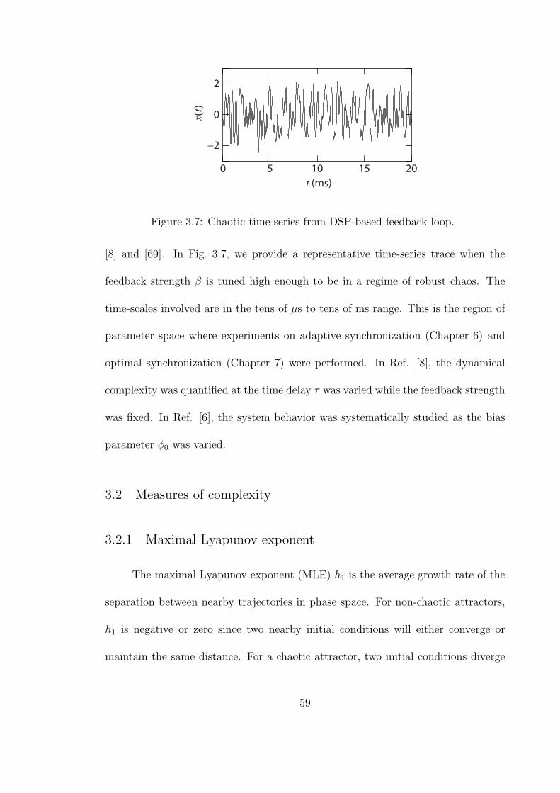
t (ms)

x(t)

0

0

2

−2

5 10 15 20

Figure 3.7: Chaotic time-series from DSP-based feedback loop.

[8] and [69]. In Fig. 3.7, we provide a representative time-series trace when the

feedback strength β is tuned high enough to be in a regime of robust chaos. The

time-scales involved are in the tens of µs to tens of ms range. This is the region of

parameter space where experiments on adaptive synchronization (Chapter 6) and

optimal synchronization (Chapter 7) were performed. In Ref. [8], the dynamical

complexity was quantified at the time delay τ was varied while the feedback strength

was fixed. In Ref. [6], the system behavior was systematically studied as the bias

parameter ϕ0 was varied.

3.2 Measures of complexity

3.2.1 Maximal Lyapunov exponent

The maximal Lyapunov exponent (MLE) h1 is the average growth rate of the

separation between nearby trajectories in phase space. For non-chaotic attractors,

h1 is negative or zero since two nearby initial conditions will either converge or

maintain the same distance. For a chaotic attractor, two initial conditions diverge

59

from one another exponentially fast, so h1 is positive. The inverse of h1 is called

the Lyapunov time and is a measure of the average time-scale for which an observed

trajectory will realistically predict the behavior of its original phase space neighbors.

For low-dimensional chaos, the MLE can be estimated from a measured scalar time-

series [70, 71]. These schemes involve constructing a phase-space of delay coordinates

and finding the average rate at which nearest neighbors diverge. This time-series

analysis method fails for high-dimensional chaos, because a finite length time-series

will include few nearby phase-space points. The conventional method for estimation

of an MLE involves integration of a linearized numerical model [72]. In this Section,

we outline this technique. In Chapter 4, we introduce a new way to estimate MLEs

that uses a hybrid of experimental time-series and nonlinear numerical modeling. In

principle, this new method could be applied in situations where there is no numerical

model but two systems can be synchronized.

Consider a continuous-time dynamical system given by the evolution equation

dz

dt= F(z). (3.1)

Our goal is to determine how points nearby to z at time t diverge as t increases.

We perform a linearization about the solution z(t) to see how a linear perturbation

δz(t) grows or decays:

dδz

dt= DF(z)δz, (3.2)

where DF is the Jacobian of F evaluated along the trajectory z(t). For a chaotic

trajectory, we expect |δz| ∼ e+h1t, and thus keep track of the growth rate as:

h1 = (t)1

tln

|δz(t)||δz(0)|

. (3.3)

60

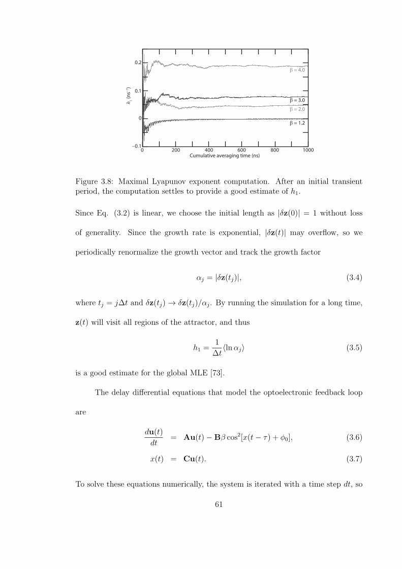
0

0

0.1

0.2

−0.1200 400 600

Cumulative averaging time (ns)

β = 1.2

β = 2.0

β = 3.0

β = 4.0

h1 (

ns−

1)

800 1000

Figure 3.8: Maximal Lyapunov exponent computation. After an initial transientperiod, the computation settles to provide a good estimate of h1.

Since Eq. (3.2) is linear, we choose the initial length as |δz(0)| = 1 without loss

of generality. Since the growth rate is exponential, |δz(t)| may overflow, so we

periodically renormalize the growth vector and track the growth factor

αj = |δz(tj)|, (3.4)

where tj = j∆t and δz(tj) → δz(tj)/αj. By running the simulation for a long time,

z(t) will visit all regions of the attractor, and thus

h1 =1

∆t⟨lnαj⟩ (3.5)

is a good estimate for the global MLE [73].

The delay differential equations that model the optoelectronic feedback loop

are

du(t)

dt= Au(t)−Bβ cos2[x(t− τ) + ϕ0], (3.6)

x(t) = Cu(t). (3.7)

To solve these equations numerically, the system is iterated with a time step dt, so

61

that the solution is available only at discrete points in time as u(j · dt) and x(j · dt).

The variational equations are:

dδu(t)

dt= Aδu(t) +Bβ sin 2[x(t− τ) + ϕ0]δx(t− τ), (3.8)

δx(t) = Cδu(t), (3.9)

which are conditional upon the solution x(t). The state of the variational mode at

time t conditional to the state x(t) is

δz(t) =

δu(t)

δx(t− dt)

δx(t− 2dt)

...

δx(t− τ)

(3.10)

which has dimensionality 14 + τ/dt− 1 where 14 is the order of the bandpass filter

and thus the linearized state space vector δu. Note that for this computation, one

must choose the time step dt to be a fraction of the round-trip delay τ . In the

same manner as described above, we compute the phase space growth as |δz(t)| to

determine the MLE h1 (| • | is the Euclidean norm).

In Fig. 3.8, we plot the growth rate h1 for different feedback strengths β as the

cumulative averaging time increases. After an initial transient period, the averaging

settles to give a good estimate of h1. The first 1 µs is plotted, but the full calculation

was performed by averaging over a total time of 10 µs.

In Fig. 3.9, we plot the calculated h1 as a function of β. At β ∼ 4, the MLE

is around 0.02 ns−1, which implies a prediction horizon time of about 50 ns or just

62

h1 (

ns–

1)

0.005

0

0.010

0.015

0.020

0.025

β

1 2 3 4 5

Figure 3.9: Maximal Lyapunov exponent computed for increasing feedbackstrengths.

over two round-trips.

3.2.2 Spectrum of Lyapunov exponents

At each point z along a chaotic orbit within its d-dimensional attractor, one can

find an orthonormal basis whose vectors are ranked in terms of their rates of phase

space expansion. The directions and growth rates vary throughout the attractor,

but the ranked set of average growth rates h1 ≥ h2 ≥ · · · ≥ hd – called the spectrum

of Lyapunov exponents (LEs) – is useful for estimating fractal dimension of a chaotic

attractor with the Kaplan-Yorke formula and for estimating the Kolmogorov-Sinai

entropy rate [73]. For chaotic motion, the largest Lyapunov exponent of this set,

is positive and strongly dominates all measures of phase space growth. Hence, h1

is the suitable metric for quantifying a system’s predictability. The sign of an LE

hk determines if a small perturbation along a particular phase space direction will

grow or decay. The number of positive LEs is a metric for chaoticity; a system with

63

at least two positive LEs is termed hyperchaotic.

To numerically calculate the spectrum of LEs from a linearized model (Eq.

(3.10)), one considers d variational equations

dδzkdt

= DF(z)δzk, (3.11)

k = 1, 2, . . . , d, where the δzk’s are initially chosen to be orthonormal vectors δzk(0)·

δzℓ(0) = 0. The set of starting states is typically chosen as

δZ(0) =

[δz1(0) δz2(0) · · · δzd(0)

]= Id (3.12)

where Id is the identity matrix. After iterating these conditional states to a time

t, one finds that each of the δzk(t)’s aligns along the direction associated with

maximal expansion. To obtain d independent growth rates with each corresponding

to a unique direction at each point in phase space, one must eliminate the role of this

preferential mode. Periodically, at time tj = j∆t, one performs a Gram-Schmidt

or QR decomposition procedure on δZ(tj) to maintain orthogonality [73]. These

routines also normalize the vectors to unity length and thus automatically provide

the growth rates α(k)j . After running the program for a long time, one calculates the

d LEs as

hk =1

∆t⟨lnα(k)

j ⟩j. (3.13)

In Ref. [74], a method based on experimental time-series analysis is presented for

extracting the spectrum of LEs. However, for a system with many positive LEs, we

have found this computation is inaccurate and often unsuccessful.

For a time-delay system, the spectrum of LEs follows much the same procedure

as for the MLE computation, by defining a phase space in terms of delay coordinates.

64

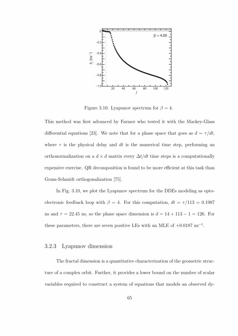
−0.2

0

20 40

j

β = 4.00

hj (

ns−

1)

60 80 100 120

−0.4

−0.6

−0.8

−1.0

Figure 3.10: Lyapunov spectrum for β = 4.

This method was first advanced by Farmer who tested it with the Mackey-Glass

differential equations [23]. We note that for a phase space that goes as d ∼ τ/dt,

where τ is the physical delay and dt is the numerical time step, performing an

orthonormalization on a d × d matrix every ∆t/dt time steps is a computationally

expensive exercise. QR decomposition is found to be more efficient at this task than

Gram-Schmidt orthogonalization [75].

In Fig. 3.10, we plot the Lyapunov spectrum for the DDEs modeling as opto-

electronic feedback loop with β = 4. For this computation, dt = τ/113 = 0.1987

ns and τ = 22.45 ns, so the phase space dimension is d = 14 + 113 − 1 = 126. For

these parameters, there are seven positive LEs with an MLE of +0.0187 ns−1.

3.2.3 Lyapunov dimension

The fractal dimension is a quantitative characterization of the geometric struc-

ture of a complex orbit. Further, it provides a lower bound on the number of scalar

variables required to construct a system of equations that models an observed dy-

65

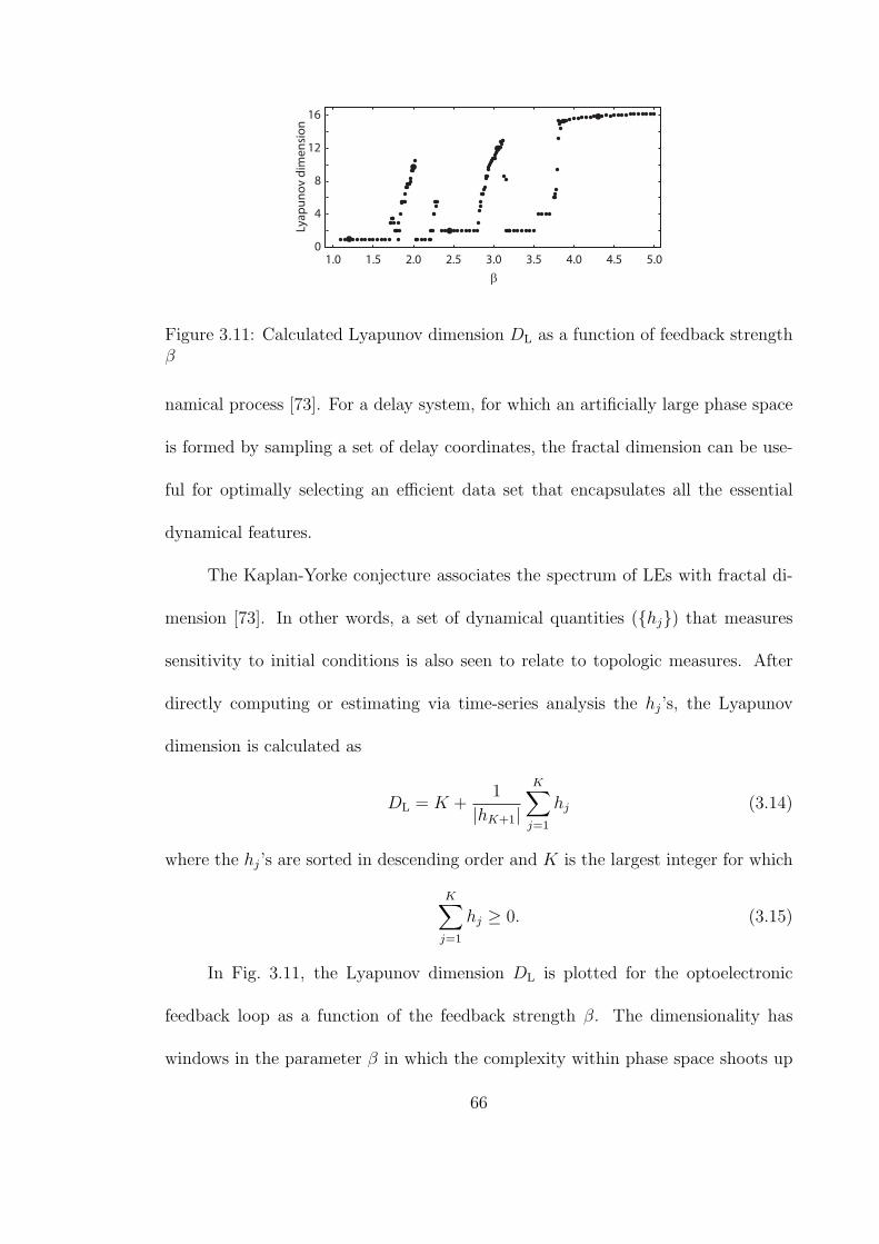
1.0 1.5 2.0 2.5 3.0 3.5 4.0 4.5 5.00

4

8

12

16

β

Lya

pu

no

v d

ime

nsi

on

Figure 3.11: Calculated Lyapunov dimension DL as a function of feedback strengthβ

namical process [73]. For a delay system, for which an artificially large phase space

is formed by sampling a set of delay coordinates, the fractal dimension can be use-

ful for optimally selecting an efficient data set that encapsulates all the essential

dynamical features.

The Kaplan-Yorke conjecture associates the spectrum of LEs with fractal di-

mension [73]. In other words, a set of dynamical quantities (hj) that measures

sensitivity to initial conditions is also seen to relate to topologic measures. After

directly computing or estimating via time-series analysis the hj’s, the Lyapunov

dimension is calculated as

DL = K +1

|hK+1|

K∑j=1

hj (3.14)

where the hj’s are sorted in descending order and K is the largest integer for which

K∑j=1

hj ≥ 0. (3.15)

In Fig. 3.11, the Lyapunov dimension DL is plotted for the optoelectronic

feedback loop as a function of the feedback strength β. The dimensionality has

windows in the parameter β in which the complexity within phase space shoots up

66

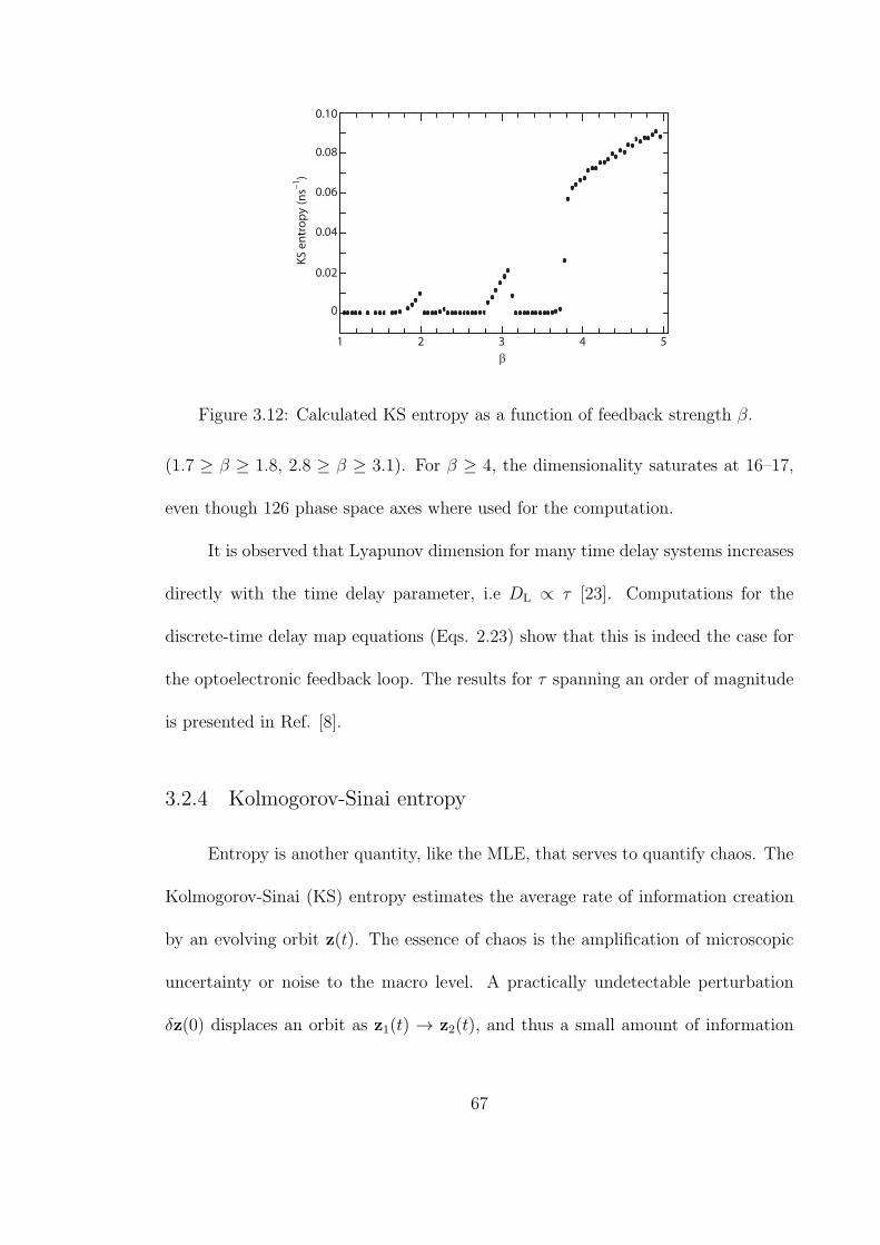
KS

en

tro

py (ns–

1)

β

1

0

0.02

0.04

0.06

0.08

0.10

2 3 4 5

Figure 3.12: Calculated KS entropy as a function of feedback strength β.

(1.7 ≥ β ≥ 1.8, 2.8 ≥ β ≥ 3.1). For β ≥ 4, the dimensionality saturates at 16–17,

even though 126 phase space axes where used for the computation.

It is observed that Lyapunov dimension for many time delay systems increases

directly with the time delay parameter, i.e DL ∝ τ [23]. Computations for the

discrete-time delay map equations (Eqs. 2.23) show that this is indeed the case for

the optoelectronic feedback loop. The results for τ spanning an order of magnitude

is presented in Ref. [8].

3.2.4 Kolmogorov-Sinai entropy

Entropy is another quantity, like the MLE, that serves to quantify chaos. The

Kolmogorov-Sinai (KS) entropy estimates the average rate of information creation

by an evolving orbit z(t). The essence of chaos is the amplification of microscopic

uncertainty or noise to the macro level. A practically undetectable perturbation

δz(0) displaces an orbit as z1(t) → z2(t), and thus a small amount of information

67

δz(0) evolves into a finite set of information (z2(t) − z1(t)). From this description,

it is seen that KS entropy is intimately related to the LEs – the rate at which

trajectories diverge. The estimate for the KS entropy rate is

hKS =∑

hj>0

hj, (3.16)

i.e. that sum of only the positive LEs [73].

In Fig. 3.12, we plot the KS entropy for the optoelectronic feedback loop.

For non-chaotic dynamics, there are no positive LEs, and hence no information is

created as time progresses. In the fully chaotic regime, the KS entropy increases to

1/(11 ns), signifying that the information expands by a fold of e every 11 ns.

KS entropy may be an important measure in the burgeoning field of random

number generation using high speed chaotic sources [7, 76, 77]. If the KS rate is fast

compared to the sampling rate, then a deterministic chaotic signal may have some

statistical properties of randomness. In fact, by threshold detecting the output

of some chaos generators, the resultant bit sequence can pass stringent tests for

randomness [7]. KS entropy may find use as a gauge for estimating how random-

like a given chaotic signal is. Unlike a true random source, which is quantum

mechanical in nature, the unpredictability of chaos is not fundamental – the state

is not a probabilistic wavefunction that collapses upon measurement but one that is

uniquely defined and completely governed by deterministic (and perhaps stochastic)

rules in which small inaccuracies compound to make the state hard to predict in

practice.

68

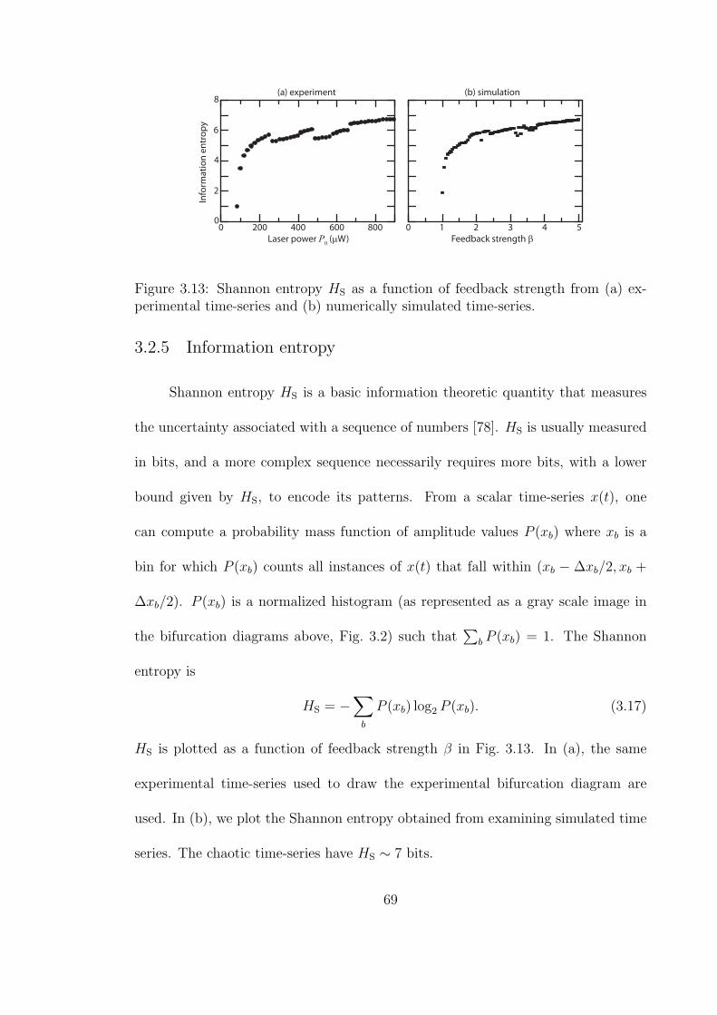
00 200 400

Laser power P0 (µW)

(a) experiment (b) simulation

Info

rma

tio

n e

ntr

op

y

Feedback strength β

600 800 0 1 2 3 4 5

2

4

6

8

Figure 3.13: Shannon entropy HS as a function of feedback strength from (a) ex-perimental time-series and (b) numerically simulated time-series.

3.2.5 Information entropy

Shannon entropy HS is a basic information theoretic quantity that measures

the uncertainty associated with a sequence of numbers [78]. HS is usually measured

in bits, and a more complex sequence necessarily requires more bits, with a lower

bound given by HS, to encode its patterns. From a scalar time-series x(t), one

can compute a probability mass function of amplitude values P (xb) where xb is a

bin for which P (xb) counts all instances of x(t) that fall within (xb − ∆xb/2, xb +

∆xb/2). P (xb) is a normalized histogram (as represented as a gray scale image in

the bifurcation diagrams above, Fig. 3.2) such that∑

b P (xb) = 1. The Shannon

entropy is

HS = −∑b

P (xb) log2 P (xb). (3.17)

HS is plotted as a function of feedback strength β in Fig. 3.13. In (a), the same

experimental time-series used to draw the experimental bifurcation diagram are

used. In (b), we plot the Shannon entropy obtained from examining simulated time

series. The chaotic time-series have HS ∼ 7 bits.

69

Information theory finds a place in nonlinear dynamics in terms of a set of

statistical tools that impart how information is shared and transferred among the

myriad variables of a dynamical systems, especially networks of coupled chaotic

oscillators. Mutual information [78] and Schrieber’s transfer entropy formulation [79]

are tools that are applicable to diagnosing connectivity strengths and directionality

of causality between interacting nodes even when there is little knowledge of the

underlying physical processes [80, 81].

3.3 Summary

1. The optoelectronic feedback loop exhibits a wide range of dynamical behaviors

as the feedback strength is varied for a fixed time delay.

2. Above a critical feedback strength, the system outputs a robust hyperchaotic

signal.

3. A numerical model based on delay differential equations shows excellent agree-

ment with experimental observations.

4. The spectrum of Lyapunov exponents provide a quantitative description of

chaotic behavior, including measures of predictability, dimensionality, and the

rate of information creation.

5. Well-controlled experiments on the complexity, predictability, and synchroniz-

ability of this prototype time-delay system can provide insights into a large

class of dynamical systems.

70

Chapter 4

Using synchronization for time-series prediction

In the preceding two chapters, it has been asserted that numerical simulations

can be made to realistically mimic the observed bifurcation sequence of an opto-

electronic feedback loop oscillator and analysis provides insights into the underlying

dynamical complexity. Synchronization is a bridge that merges the overlapping ap-

proaches of experimentation, simulation, and analysis for powerful and practical

applications. Using synchronization, we can finely tune simulation parameters to

match experimental settings, precisely set the current state, and make accurate fore-

casts of future yet unobserved states. In this Chapter, we present a method that

drives a computer model into synchrony with a recorded oscilloscope time trace by

detecting the proper system parameters and constructing the full multidimensional

state from only the observed scalar variable. After a complete oscilloscope acqui-

sition data stream is injected into the model, the reconstructed state can be used

as an initial condition for an independently run model. The model is designed to

predict the next states of the real experimental system. By comparing the real out-

put with predictions, we measure as the error increases and the solutions diverge.

A wide distribution of divergence rates implies that predictability varies through-

out a chaotic attractor with some initial conditions more amenable to predictions

than others. This experiment-to-simulation synchronization method quantifies local

71

predictability within a specific phase space region of interest, namely the current

location. This method relies on a mathematical model standing in as a numerical

replica of a second dynamical system. We also show that a secondary experimental

feedback loop can predict the time evolution of a primary loop. Hence, experiment-

to-experiment synchrony is used to make predictions even when no mathematical

model is available.

4.1 Open loop synchronization

For a given set of system parameters, a long time-series V1(t) is recorded on a

high-speed digital oscilloscope. The data sequence is obtained by an 8-bit analog-to-

digital converter at the oscilloscope’s input. Thus the signal is sampled as V1(n ·TS)

where Ts = 1/fs is the sampling interval and with a finite resolution quantized into

256 discrete voltage levels. Only a subset of the 256 levels are occupied, yielding

a more realistic resolution of about 7 bits. Furthermore, the samples V1(n · Ts)

include not only the desired dynamical signal but also a superposition of additive

analog noise terms, which encompass 5 to 10 percent of the records, with the noise

amplitude growing with oscilloscope bandwidth. It is a challenge to incorporate

these limited and noisy observations into a numerical model.

For the experimental time-series presented in Chapter 3, the sampling rate was

Ts = 0.1 ns and the total record length was 50 µs. The numerical simulation were

run with a time step of dt = 0.005 ns with a fifth-order fixed step Dormand-Prince

DDE solver. When the oscilloscope time-series are read into the computer, the data

72

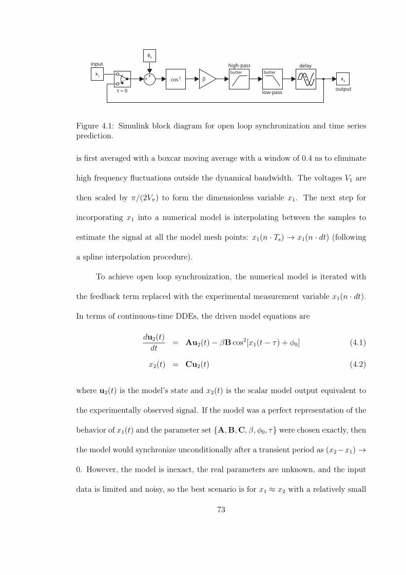
cos 2 β

φ0

butter butter

x2

++

delay

output

x1

input high-pass

t = 0 low-pass

Figure 4.1: Simulink block diagram for open loop synchronization and time seriesprediction.

is first averaged with a boxcar moving average with a window of 0.4 ns to eliminate

high frequency fluctuations outside the dynamical bandwidth. The voltages V1 are

then scaled by π/(2Vπ) to form the dimensionless variable x1. The next step for

incorporating x1 into a numerical model is interpolating between the samples to

estimate the signal at all the model mesh points: x1(n · Ts) → x1(n · dt) (following

a spline interpolation procedure).

To achieve open loop synchronization, the numerical model is iterated with

the feedback term replaced with the experimental measurement variable x1(n · dt).

In terms of continuous-time DDEs, the driven model equations are

du2(t)

dt= Au2(t)− βB cos2[x1(t− τ) + ϕ0] (4.1)

x2(t) = Cu2(t) (4.2)

where u2(t) is the model’s state and x2(t) is the scalar model output equivalent to

the experimentally observed signal. If the model was a perfect representation of the

behavior of x1(t) and the parameter set A,B,C, β, ϕ0, τ were chosen exactly, then

the model would synchronize unconditionally after a transient period as (x2−x1) →

0. However, the model is inexact, the real parameters are unknown, and the input

data is limited and noisy, so the best scenario is for x1 ≈ x2 with a relatively small

73

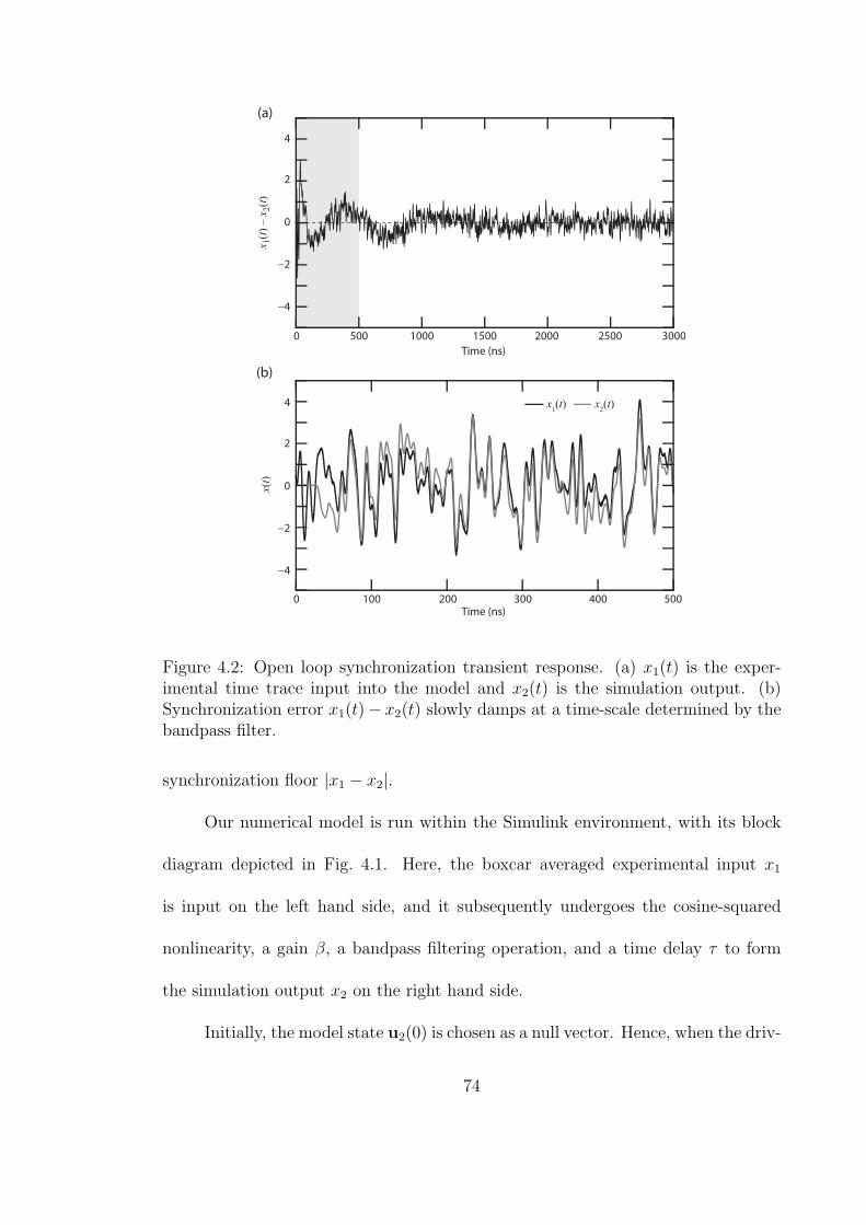
0

0

2

−2

−4

4

(b)

(a)

0

2

−2

−4

4

0

100 200

Time (ns)

x(t

)

x1(t)

Time (ns)

300 400 500

500 1000 1500 2000 2500 3000

x1(t

) – x

2(t

)

x2(t)

Figure 4.2: Open loop synchronization transient response. (a) x1(t) is the exper-imental time trace input into the model and x2(t) is the simulation output. (b)Synchronization error x1(t)− x2(t) slowly damps at a time-scale determined by thebandpass filter.

synchronization floor |x1 − x2|.

Our numerical model is run within the Simulink environment, with its block

diagram depicted in Fig. 4.1. Here, the boxcar averaged experimental input x1

is input on the left hand side, and it subsequently undergoes the cosine-squared

nonlinearity, a gain β, a bandpass filtering operation, and a time delay τ to form

the simulation output x2 on the right hand side.

Initially, the model state u2(0) is chosen as a null vector. Hence, when the driv-

74

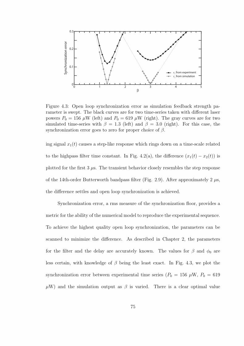
0 1 2

β

Syn

chro

niz

ati

on

err

or

x1 from experiment

x1 from simulation

0

0.1

0.2

0.3

3 4 5

Figure 4.3: Open loop synchronization error as simulation feedback strength pa-rameter is swept. The black curves are for two time-series taken with different laserpowers P0 = 156 µW (left) and P0 = 619 µW (right). The gray curves are for twosimulated time-series with β = 1.3 (left) and β = 3.0 (right). For this case, thesynchronization error goes to zero for proper choice of β.

ing signal x1(t) causes a step-like response which rings down on a time-scale related

to the highpass filter time constant. In Fig. 4.2(a), the difference (x1(t) − x2(t)) is

plotted for the first 3 µs. The transient behavior closely resembles the step response

of the 14th-order Butterworth bandpass filter (Fig. 2.9). After approximately 2 µs,

the difference settles and open loop synchronization is achieved.

Synchronization error, a rms measure of the synchronization floor, provides a

metric for the ability of the numerical model to reproduce the experimental sequence.

To achieve the highest quality open loop synchronization, the parameters can be

scanned to minimize the difference. As described in Chapter 2, the parameters

for the filter and the delay are accurately known. The values for β and ϕ0 are

less certain, with knowledge of β being the least exact. In Fig. 4.3, we plot the

synchronization error between experimental time series (P0 = 156 µW, P0 = 619

µW) and the simulation output as β is varied. There is a clear optimal value

75

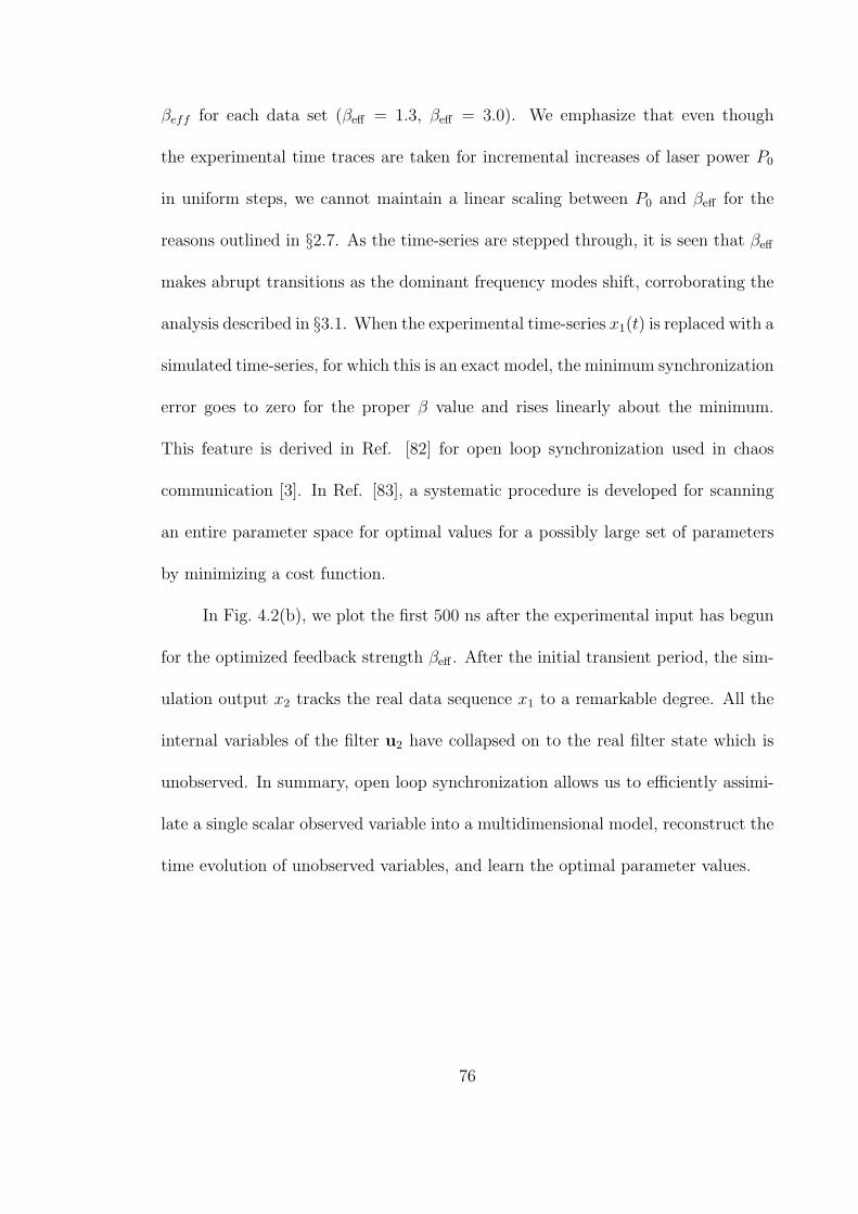
βeff for each data set (βeff = 1.3, βeff = 3.0). We emphasize that even though

the experimental time traces are taken for incremental increases of laser power P0

in uniform steps, we cannot maintain a linear scaling between P0 and βeff for the

reasons outlined in §2.7. As the time-series are stepped through, it is seen that βeff

makes abrupt transitions as the dominant frequency modes shift, corroborating the

analysis described in §3.1. When the experimental time-series x1(t) is replaced with a

simulated time-series, for which this is an exact model, the minimum synchronization

error goes to zero for the proper β value and rises linearly about the minimum.

This feature is derived in Ref. [82] for open loop synchronization used in chaos

communication [3]. In Ref. [83], a systematic procedure is developed for scanning

an entire parameter space for optimal values for a possibly large set of parameters

by minimizing a cost function.

In Fig. 4.2(b), we plot the first 500 ns after the experimental input has begun

for the optimized feedback strength βeff . After the initial transient period, the sim-

ulation output x2 tracks the real data sequence x1 to a remarkable degree. All the

internal variables of the filter u2 have collapsed on to the real filter state which is

unobserved. In summary, open loop synchronization allows us to efficiently assimi-

late a single scalar observed variable into a multidimensional model, reconstruct the

time evolution of unobserved variables, and learn the optimal parameter values.

76

4.2 Time-series prediction

For each experimental time trace x1(t) recorded at a different laser power P0,

we find there is a feedback strength βeff for which the simulation output becomes

well-entrained to the experimental input, i.e. x2(t) ≈ x1(t). After open loop syn-

chronization is achieved, the next step is to terminate the external drive signal to

the simulation and to replace it with its internal copy. At a specific time, the feed-

back term is ‘switched’ from −β cos2[x1(t− τ) + ϕ0] to −β cos2[x2(t− τ) + ϕ0]. We

denote the switch time t = 0; however, we may perform the switch at any time.

In practice, we choose the switch event to occur within time windows where the

synchronization error |x1 − x2| is relatively small. After t = 0, the simulation runs

completely independently. In Fig. 4.1, the switch block represents the exchange of

feedback variables at t = 0 in the Simulink simulation.

The simulation iterates x2(t) for t > 0 continue to track the real experimental

observations. The model is able to predict states for which it does not directly

have access, both in terms of the scalar output variable x1 and the internal states

u1. The term ‘predict’ is used somewhat loosely in that the real data has already

been acquired and stored and the simulations do not necessarily run faster than

real-time. Nevertheless, we regard this exercise is a proof-of-principle test of this

simulation-prediction scheme.

For non-chaotic orbits, we expect that a closely entrained initial state will

continue to track its driver even after the drive term has been discontinued. In

Figs. 4.4 (a)–(f), we plot the pair of time-series x1(t) and x2(t) after t = 0. Indeed,

77

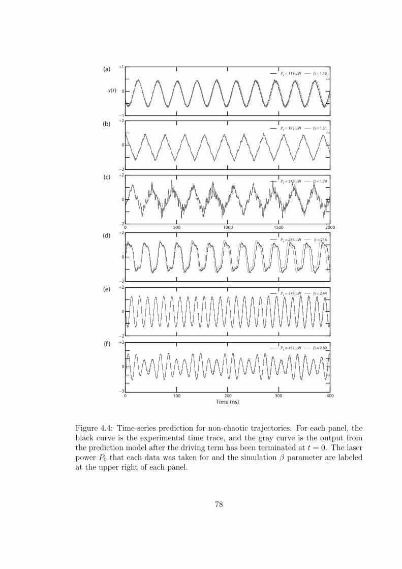
0

P0 = 119 µW

(a)+1

−1

x(t)

0

+2

−2

0

0

+2

−2500 1000 1500 2000

0

+2

−2

0

+2

−2

0

0

+3

−3100 200

Time (ns)

300 400

β = 1.13

P0 = 193 µW

(b)β = 1.51

P0 = 249 µW

(c)β = 1.79

P0 = 286 µW

(d)β = 216

P0 = 378 µW

(e)β = 2.44

P0 = 452 µW

(f )β = 2.80

Figure 4.4: Time-series prediction for non-chaotic trajectories. For each panel, theblack curve is the experimental time trace, and the gray curve is the output fromthe prediction model after the driving term has been terminated at t = 0. The laserpower P0 that each data was taken for and the simulation β parameter are labeledat the upper right of each panel.

78

x(t) 0

+2

−2

0

+2

−2

x 1(t)−x 2(t)

0

10 10

1

0.1

0.1

0.01

0.001

1

+4

+2

−4

−2

0

+4

+2

−4

−2

−200 0

Time (ns)

Experiment Simulation(a)

(b)

(c)

(d)

(e)

(f )

|x1(t)−x 2(t)|

200 400 −200 0

Time (ns)200 400 600

Figure 4.5: Time-series prediction for chaotic trajectories. (a) Results from exper-imental time-series x1(t). For t < 0, the model output x2(t) is driven by the inputx1(t), and for t > 0, the model providing predictions. The difference grows remainssmall for t < 0 and grows exponentially for t > 0. (b) Corresponding results forx1(t) from simulation.

79

−3−3

−2

−2

−1

−1

0

0

1

1

2

2

3

3(a) experiment

−400 ns < t ≤ 0

simulation(c)

x1(t)

x2(t)

−3−3

−2

−2

−1

−1

0

0

1

1

2

2

3

3

x1(t)

x2(t)

−3−3

−2

−2

−1

−1

0

0

1

1

2

2

3

3(b) (d)

x1(t)

x2(t)

−3−3

−2

−2

−1

−1

0

0

1

1

2

2

3

3

x1(t)

x2(t)

−400 ns < t ≤ 0

0 < t < 1 µs 0 < t < 1 µs

Figure 4.6: Synchronization plots during open loop synchronization and divergence.(a,c) t < 0, (b,d) t > 0.

80

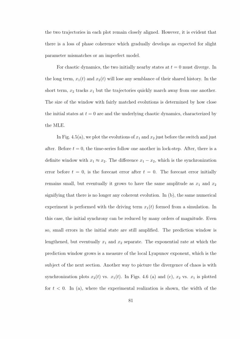
the two trajectories in each plot remain closely aligned. However, it is evident that

there is a loss of phase coherence which gradually develops as expected for slight

parameter mismatches or an imperfect model.

For chaotic dynamics, the two initially nearby states at t = 0 must diverge. In

the long term, x1(t) and x2(t) will lose any semblance of their shared history. In the

short term, x2 tracks x1 but the trajectories quickly march away from one another.

The size of the window with fairly matched evolutions is determined by how close

the initial states at t = 0 are and the underlying chaotic dynamics, characterized by

the MLE.

In Fig. 4.5(a), we plot the evolutions of x1 and x2 just before the switch and just

after. Before t = 0, the time-series follow one another in lock-step. After, there is a

definite window with x1 ≈ x2. The difference x1 − x2, which is the synchronization

error before t = 0, is the forecast error after t = 0. The forecast error initially

remains small, but eventually it grows to have the same amplitude as x1 and x2

signifying that there is no longer any coherent evolution. In (b), the same numerical

experiment is performed with the driving term x1(t) formed from a simulation. In

this case, the initial synchrony can be reduced by many orders of magnitude. Even

so, small errors in the initial state are still amplified. The prediction window is

lengthened, but eventually x1 and x2 separate. The exponential rate at which the

prediction window grows is a measure of the local Lyapunov exponent, which is the

subject of the next section. Another way to picture the divergence of chaos is with

synchronization plots x2(t) vs. x1(t). In Figs. 4.6 (a) and (c), x2 vs. x1 is plotted

for t < 0. In (a), where the experimental realization is shown, the width of the

81

data points about the line x2 = x1 is a gauge of the synchronization error between

experiment and simulation. In (c), where x1 comes from simulation, the data fall

almost exactly on the x2 = x1 line. In (b) and (d), the orbits are plotted for t > 0.

In this case, there is an initial set of points along the synchronization line, but the

majority of points fall far off the line.

4.3 Prediction horizon times and distribution of finite time Lyapunov

exponents

The exponential rate of divergence between the signals x1(t) and x2(t) is an

estimate of the local MLE h1. The multiplicative inverse of h1 is the characteristic

time-scale for which we can make accurate prediction, called the prediction horizon

time. For a diverging pair, we can extract the prediction horizon time by finding

the best fit line on a plot of ln⟨|x1−x2|⟩ where ⟨•⟩ denotes a boxcar moving average

with a window of length 25 ns which is performed to rid inaccuracies due to zero

crossing in x1−x2. In Fig. 4.5(a), the lower pane depicts this exponential divergence

as a line with positive slope on a semilogarithmic axis. The fit is only performed on

a finite time window T since the prediction error saturates when the solutions x1

and x2 are as far away as possible on the bound attractor. In this case, we fit from

t = 25 ns to t = 75 ns. In the lower pane of (b), the divergence is plotted in the

same manner for an example of simulation-simulation synchronization. In this case,

the initial error is much smaller, so the solutions take longer to reach saturation.

However, we make the linear fit over the same window to make a comparison with

82

250

0.01

0.02

0.03

0.04

0.05

0.06

0.07

0.08

50

Prediction horizon (ns)

75 100 125 150

Pro

ba

bili

ty

from experiment

from simulation

Figure 4.7: Distribution of prediction horizon times for β = 4.0. Results from usingx1 as an experimental time trace and a simulated time trace are compared.

the experiment-simulation results.

The same numerical exercise can be repeated many times by choosing the

switch event as different points in the time-series x1(t). Both the initial error level

and the rate of divergence varies for each trial. We study the distribution of diver-

gence rates in more detail. In Fig. 4.7, we plot a histogram of prediction horizon

times for βeff = 4.0. For some trials, the experimental time-series can be reliably

forecast for a period of greater than 100 ns or about four complete round-trips;

while most initial states allow for forecasts of around 35 ns. The same computation

was repeated with a simulation time-series for x1(t) and β = βeff . The distribu-

tions of horizon times agree very well. We conclude that the statistics regarding

predictability can be ascertained using the experiment-simulation synchronization

method.

In simulation, we may vary the window T over which the exponential relation

is fit. There is a well-known relationship between the width of the distribution of

83

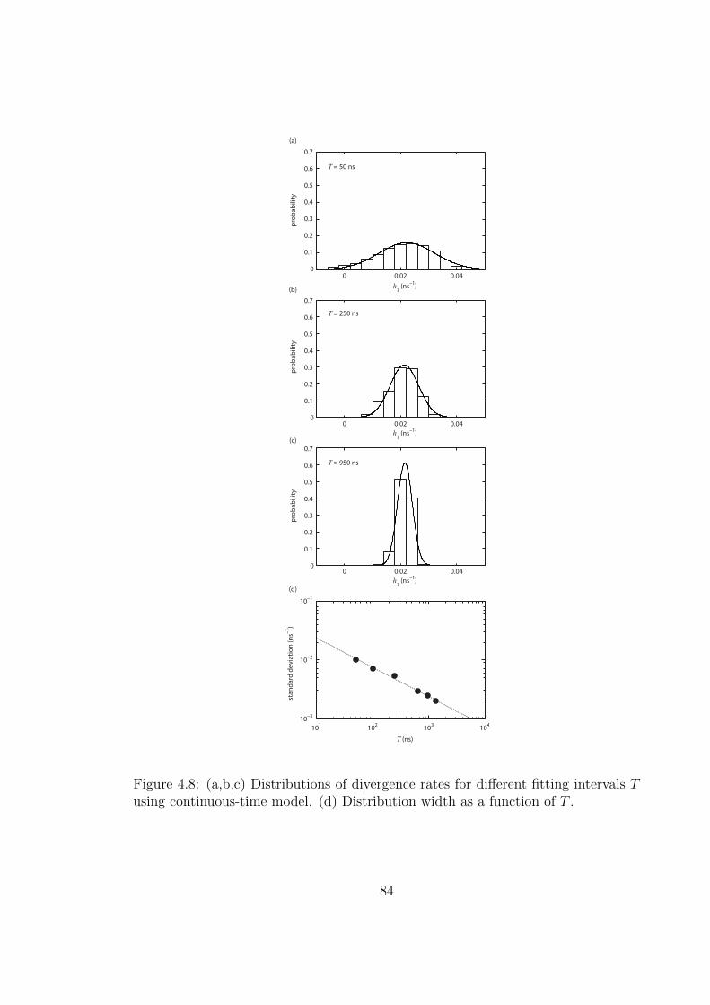
0 0.02 0.04

0 0.02 0.04

0 0.02 0.04

0

0.1

0.2

0.3

0.4

0.5

0.6

0.7

0

0.1

0.2

0.3

0.4

0.5

0.6

0.7

0

0.1

0.2

0.3

0.4

0.5

0.6

0.7

h1 (ns

–1)

h1 (ns

–1)

h1 (ns

–1)

T (ns)

pro

ba

bil

ity

pro

ba

bil

ity

pro

ba

bil

ity

sta

nd

ard

de

via

tio

n (

ns–

1)

(a)

(b)

(c)

(d)

T = 50 ns

T = 250 ns

T = 950 ns

10–3

101

102

103

104

10–1

10–2

Figure 4.8: (a,b,c) Distributions of divergence rates for different fitting intervals Tusing continuous-time model. (d) Distribution width as a function of T .

84

103

102

101

0 1 2 3 4

rate (ms−1)F

req

ue

nc

y

h1

T = 8 ms

T = 4 ms

T = 2 ms

Figure 4.9: Distribution of divergence rates for different fitting intervals usingdiscrete-time model.

finite-time Lyapunov exponents P (h1, T ) and the fit time T . In particular, P (h1, T )

follows a Gaussian distribution with a mean equal to the globally averaged MLE

h1 and a standard deviation σ which goes as 1/√T [73]. In the limit T → ∞, the

distribution narrows to a delta peak at h1 = h1. In effect, this means that the

measurement is performed such that the trajectories x1 and x2 traverse all regions

of the attractor. Structural effects of the chaotic attractor make the distribution

deviate from the Gaussian shape in the tails far from h1. A comprehensive treatment

of this feature is examined in Ref. [43, 84]. In Fig. 4.8 (a)–(c), we plot histograms

P (h1, T ) for fit time T = 50, 250 and 950 ns along with the best fit Gaussian. In (d),

the standard deviation is plotted as a function T and the σ ∼ T−1/2 relationship is

recovered.

The same sort of time-series based divergence rate evaluations were executed

for the discrete-time map model (§2.11). In this case, the time-scales involved are

orders of magnitude slower, in the ms rather than ns range. Here, the calculations are

repeated 105 times. The distribution of h1 ∼ ln⟨|x1[n]−x2[n]|⟩ is plotted for different

85

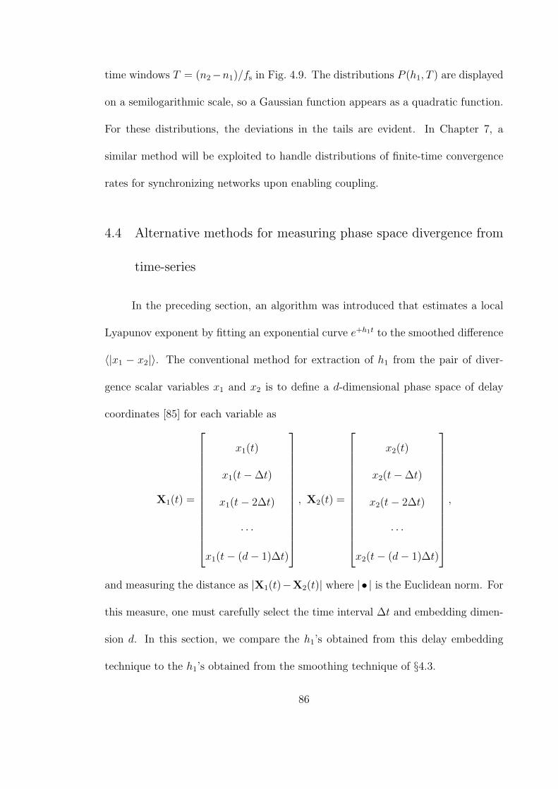
time windows T = (n2−n1)/fs in Fig. 4.9. The distributions P (h1, T ) are displayed

on a semilogarithmic scale, so a Gaussian function appears as a quadratic function.

For these distributions, the deviations in the tails are evident. In Chapter 7, a

similar method will be exploited to handle distributions of finite-time convergence

rates for synchronizing networks upon enabling coupling.

4.4 Alternative methods for measuring phase space divergence from

time-series

In the preceding section, an algorithm was introduced that estimates a local

Lyapunov exponent by fitting an exponential curve e+h1t to the smoothed difference

⟨|x1 − x2|⟩. The conventional method for extraction of h1 from the pair of diver-

gence scalar variables x1 and x2 is to define a d-dimensional phase space of delay

coordinates [85] for each variable as

X1(t) =

x1(t)

x1(t−∆t)

x1(t− 2∆t)

· · ·

x1(t− (d− 1)∆t)

, X2(t) =

x2(t)

x2(t−∆t)

x2(t− 2∆t)

· · ·

x2(t− (d− 1)∆t)

,

and measuring the distance as |X1(t)−X2(t)| where | • | is the Euclidean norm. For

this measure, one must carefully select the time interval ∆t and embedding dimen-

sion d. In this section, we compare the h1’s obtained from this delay embedding

technique to the h1’s obtained from the smoothing technique of §4.3.

86

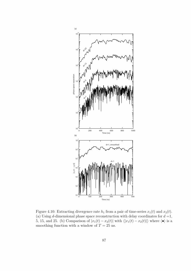
10

10

10

10

10

10

10

-2

0

2

4

6

8

10

0 200 400 600 800 1000

0 100 200 300 400 50010

-3

10-2

10-1

100

101

102

103

Time (ns)

Time (ns)

ph

ase

sp

ace

se

par

atio

n

d=1d=5

d=15d=25

d=1

d=1, smoothed

|x1(t

) –

x2(t

)|

(a)

(b)

Figure 4.10: Extracting divergence rate h1 from a pair of time-series x1(t) and x2(t).(a) Using d-dimensional phase space reconstruction with delay coordinates for d =1,5, 15, and 25. (b) Comparison of |x1(t)− x2(t)| with ⟨|x1(t)− x2(t)|⟩ where ⟨•⟩ is asmoothing function with a window of T = 25 ns.

87

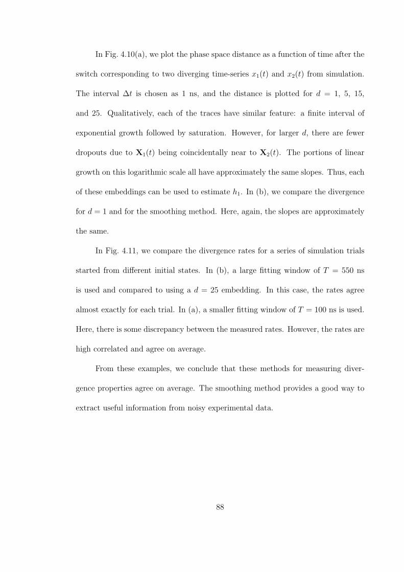
In Fig. 4.10(a), we plot the phase space distance as a function of time after the

switch corresponding to two diverging time-series x1(t) and x2(t) from simulation.

The interval ∆t is chosen as 1 ns, and the distance is plotted for d = 1, 5, 15,

and 25. Qualitatively, each of the traces have similar feature: a finite interval of

exponential growth followed by saturation. However, for larger d, there are fewer

dropouts due to X1(t) being coincidentally near to X2(t). The portions of linear

growth on this logarithmic scale all have approximately the same slopes. Thus, each

of these embeddings can be used to estimate h1. In (b), we compare the divergence

for d = 1 and for the smoothing method. Here, again, the slopes are approximately

the same.

In Fig. 4.11, we compare the divergence rates for a series of simulation trials

started from different initial states. In (b), a large fitting window of T = 550 ns

is used and compared to using a d = 25 embedding. In this case, the rates agree

almost exactly for each trial. In (a), a smaller fitting window of T = 100 ns is used.

Here, there is some discrepancy between the measured rates. However, the rates are

high correlated and agree on average.

From these examples, we conclude that these methods for measuring diver-

gence properties agree on average. The smoothing method provides a good way to

extract useful information from noisy experimental data.

88

−0.01−0.01

0

0

0.01

Divergence rate, d = 25 embedding (ns−1)

(a) !t time: 50 ns to 150 ns

Div

erg

en

ce r

ate

, tim

e a

ve

rag

ing

(n

s−1)

0.01

0.02

0.02

0.03

0.03

0.04

0.04

−0.01−0.01

0

0

0.01

Divergence rate, d = 25 embedding (ns−1)

(b) !t time: 50 ns to 600 ns

Div

erg

en

ce r

ate

, tim

e a

ve

rag

ing

(n

s−1)

0.01

0.02

0.02

0.03

0.03

0.04

0.04

Figure 4.11: Comparison of extracted divergence rates h1 using different methods.(a) Smoothing over 100 ns vs. a 25-dimensional delay phase space. (b) Smoothingover 550 ns vs. a 25-dimensional phase space.

4.5 Measured maximal Lyapunov exponents

The local LE h1 for a pair of diverging trajectories measures the predictability

in the region of phase space nearby to (u2(t), x2(t), x2(t−∆t), . . . , x2(t− τ)). The

distribution of local LEs P (h1, T ) provides statistics regarding the variation of pre-

dictability throughout the entire attractor. The mean of the distribution h1 is an

estimate of the global MLE – how initial conditions diverge on average. By repeat-

ing the synchronization-release experiment many times under different experimental

conditions, we can measure the MLEs as a function of the feedback strength β. In

Fig. 4.12, we plot the MLEs obtained through this hybrid experiment-simulation

method along with the MLEs derives from direct computation of a linearized model

(§3.2.1). The open circles are the estimates from x1(t) being an experimental time

trace, and the open squares are from when x1(t) is a simulated time trace. All three

89

h1 (

ns–

1)

0.005

0

0.010

0.015

0.020

0.025

β

1 2 3 4 5

from experiment

from simulation

direct calculation

Figure 4.12: Average divergence rate h1 vs. feedback strength β.

sets of points overlap reasonably well. We conclude that this technique based on

open loop synchronization is a new way to estimate global properties of a chaotic

system. It attains an important balance between the application of real-world data

streams and numerical modeling.

4.6 Prediction using a secondary experimental system

The routine described in this chapter can be applied even when there is no

accurate numerical model for the chaotic dynamics under test. If two coupled sys-

tems can be forced into a synchronous state, then the properties of an isolated

system’s MLE can be experimentally measured. By synchronizing and subsequently

interrupting the communication link, while simultaneously recording a scalar out-

put variable from each system, the divergence rate can be extracted. By repeating

this synchronization-then-release procedure many times, the measured distribution

of h1’s can yield the global MLE h1 which characterized the underlying chaotic mo-

90

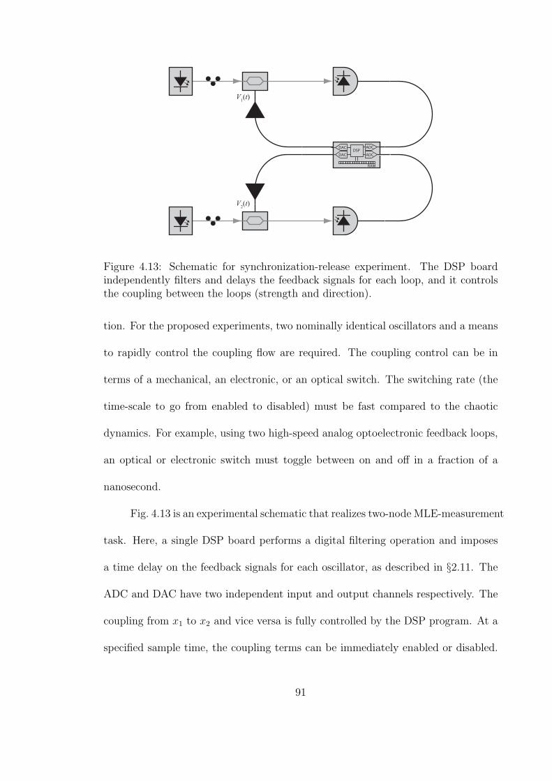
V1(t)

V2(t)

ADCDAC

DSP

RAM

DAC ADC

Figure 4.13: Schematic for synchronization-release experiment. The DSP boardindependently filters and delays the feedback signals for each loop, and it controlsthe coupling between the loops (strength and direction).

tion. For the proposed experiments, two nominally identical oscillators and a means

to rapidly control the coupling flow are required. The coupling control can be in

terms of a mechanical, an electronic, or an optical switch. The switching rate (the

time-scale to go from enabled to disabled) must be fast compared to the chaotic

dynamics. For example, using two high-speed analog optoelectronic feedback loops,

an optical or electronic switch must toggle between on and off in a fraction of a

nanosecond.

Fig. 4.13 is an experimental schematic that realizes two-node MLE-measurement

task. Here, a single DSP board performs a digital filtering operation and imposes

a time delay on the feedback signals for each oscillator, as described in §2.11. The

ADC and DAC have two independent input and output channels respectively. The

coupling from x1 to x2 and vice versa is fully controlled by the DSP program. At a

specified sample time, the coupling terms can be immediately enabled or disabled.

91

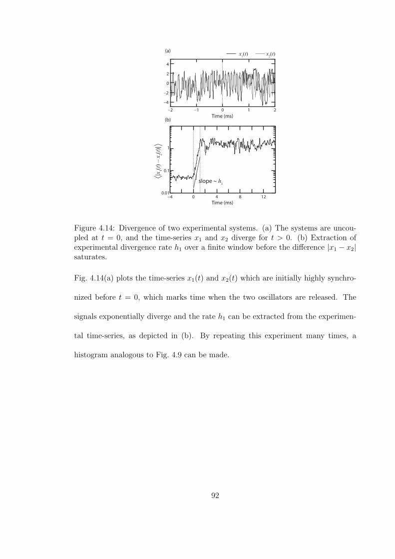
(a)

(b)

4

2

0

−2

−4

x1(t) x

2(t)

1

0.1

0.01

|x1(t

) – x

2(t

)|

−2 −1 0 1 2

Time (ms)

Time (ms)0 4 8 12−4

slope ∼ h1

Figure 4.14: Divergence of two experimental systems. (a) The systems are uncou-pled at t = 0, and the time-series x1 and x2 diverge for t > 0. (b) Extraction ofexperimental divergence rate h1 over a finite window before the difference |x1 − x2|saturates.

Fig. 4.14(a) plots the time-series x1(t) and x2(t) which are initially highly synchro-

nized before t = 0, which marks time when the two oscillators are released. The

signals exponentially diverge and the rate h1 can be extracted from the experimen-

tal time-series, as depicted in (b). By repeating this experiment many times, a

histogram analogous to Fig. 4.9 can be made.

92

4.7 Summary

1. Open loop synchronization of a numerical model to experimental observations

is a data assimilation and parameter estimation technique.

2. A computer simulation initialized via open loop synchronization can make

reliable forecast of high dimensional chaos.

3. The prediction horizon time varies with initial condition.

4. The maximal Lyapunov exponent can be ascertained by driving two systems

into nearby phase space trajectories (by synchronization) and then observing

their divergence upon terminating the coupling.

5. In principle, a replica experimental system can be used for measuring the

distribution of local Lyapunov exponents.

93

Chapter 5

Anticipated synchronization

When two or more spatially-separated dynamical systems interact over chan-

nels that transmit signals at a finite speed, the network may exhibit achronal syn-

chronization patterns. For example, a pair of bidirectionally coupled chaotic oscil-

lators with a coupling delay τC may have a strong correlation at a time shift of τC

and weak or no correlation at zero lag [86, 87, 88]. Detecting if a unique leader

and follower relationship exists is a challenge, and there is evidence, in fact, that

the role of each node can switch randomly [50]. Extrapolating from this two-node

result, it may be expected that a large network of N chaotic oscillators with each

coupling link having a nonuniform time delay τij will exhibit an even more compli-

cated dance, perhaps forming clusters that jump in and out of lagged synchrony.

Thus, observations of long-range isochronal synchrony in neuronal systems [89, 90] is

surprising and have been a source of motivation for numerous analytical [91, 92, 93],

numerical [49], and experimental [48, 94] studies over the past decade. An under-

standing of how nature is arranged or how we may arrange nature such that stable

zero-lag synchrony is maintained over long distances is useful from a fundamental

perspective in regards to information processing in the brain and for applied pur-

poses such as communication networks. A parallel focus over the past decade has

been to elucidate the mechanisms responsible for anticipated synchrony – an intrigu-

94

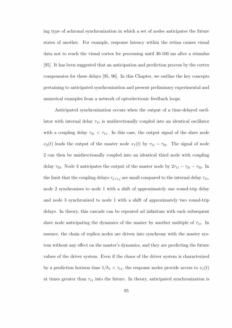
ing type of achronal synchronization in which a set of nodes anticipates the future

states of another. For example, response latency within the retina causes visual

data not to reach the visual cortex for processing until 30-100 ms after a stimulus

[95]. It has been suggested that an anticipation and prediction process by the cortex

compensates for these delays [95, 96]. In this Chapter, we outline the key concepts

pertaining to anticipated synchronization and present preliminary experimental and

numerical examples from a network of optoelectronic feedback loops.

Anticipated synchronization occurs when the output of a time-delayed oscil-

lator with internal delay τ11 is unidirectionally coupled into an identical oscillator

with a coupling delay τ21 < τ11. In this case, the output signal of the slave node

x2(t) leads the output of the master node x1(t) by τ11 − τ21. The signal of node

2 can then be unidirectionally coupled into an identical third node with coupling

delay τ32. Node 3 anticipates the output of the master node by 2τ11 − τ21 − τ32. In

the limit that the coupling delays τj+1,j are small compared to the internal delay τ11,

node 2 synchronizes to node 1 with a shift of approximately one round-trip delay

and node 3 synchronized to node 1 with a shift of approximately two round-trip

delays. In theory, this cascade can be repeated ad infinitum with each subsequent

slave node anticipating the dynamics of the master by another multiple of τ11. In

essence, the chain of replica nodes are driven into synchrony with the master sys-

tem without any effect on the master’s dynamics, and they are predicting the future

values of the driver system. Even if the chaos of the driver system is characterized

by a prediction horizon time 1/h1 < τ11, the response nodes provide access to x1(t)

at times greater than τ11 into the future. In theory, anticipated synchronization is

95

able to enhance the attainable prediction horizon to an arbitrarily long time. By

replacing the identical replica nodes with a chain of numerical models, a computer

can continuously predict the future states of the experimental system far in advance.

In practice, there is a limit to how far into the future a chaotic oscillator’s output

can be reliably forecast using this anticipated synchronization scheme. Perturba-

tions, mismatches, and noise propagate and intensify along the path of cascaded

nodes, whether the nodes are physical or numerical. Since unidirectional coupling

is employed, there is no chance for recovery as there would be for a bidirectional

array.

The notion of anticipated synchronization was first advanced by Voss in Refs.

[59] and [97]. The first experimental measurements on time-delayed electronic os-

cillators were also performed by Voss [98]. Experimental investigations have been

published using a unidirectionally coupled pair of chaotic semiconductor lasers [99]

and numerical models demonstrate anticipated synchronization for coupled neurons

[100]. Stability of anticipated synchronization is the subject of Ref. [101]. Studies

have considered the applicability of anticipated synchronization to the prediction

problem [102] and the parameter estimation problem [103].

5.1 Anticipated synchronization between three optoelectronic feed-

back loops

As an experimental demonstration of anticipated synchronization of high-

dimensional chaotic oscillators, we consider a closed loop optoelectronic feedback

96

loop as a master system and two cascaded open loop systems as slaves. The param-

eters of each loop, including the laser powers, half-wave voltages, and amplification

factors, are tuned to be nominally identical. The electronic bandwidth is 1–100

MHz and the effective feedback strengths are β ≈ 4. The internal feedback delay of

the driver loop is τ11 = 72 ns. Fig. 5.1 is a schematic of this setup. The modulation

voltage of the master loop V1(t) is split off to also act as a coupling signal for the

second node. The coupling delay τ21 is chosen to be smaller than τ11. Note that

the coupling signal may also be transmitted via an optical fiber by using an optical

1 × 2 splitter at node 1. The output voltage of the second node V2(t) is used as a

modulation voltage for the third node, which outputs a voltage signal V3(t). The

signals V1(t), V2(t), and V3(t) are observed on a fast oscilloscope. The communica-

tion delays are distributed throughout the network, and are estimated to be τ21 = 36

ns and τ32 = 36 ns.

In Fig. 5.2, we plot the normalized time-series x1(t), x2(t), and x3(t) measured

simultaneously. There are obvious time-shifted correlations in the temporal patterns

within the three signals; the dashed lines highlight some analogous features that

appear in each time-series. In Fig. 5.3, we plot (a) the autocorrelation of x1(t), (b)

the cross-correlation between x1(t) and x2(t), and (c) the cross-correlation between

x1(t) and x3(t). All of these are normalized such that an autocorrelation equals

1 at zero lag. In (a), we find that the dynamics of isolated feedback loop with

this parameter set has time-domain structure dictated by the round-trip time since

there are strong peaks at ±τ11 = ±72 ns. Plot (b) confirms that x2 leads x1 by

∆T2 = τ11 − τ21 = 36 ns such that x2(t) ≈ x1(t+∆T2). The correlation coefficient

97

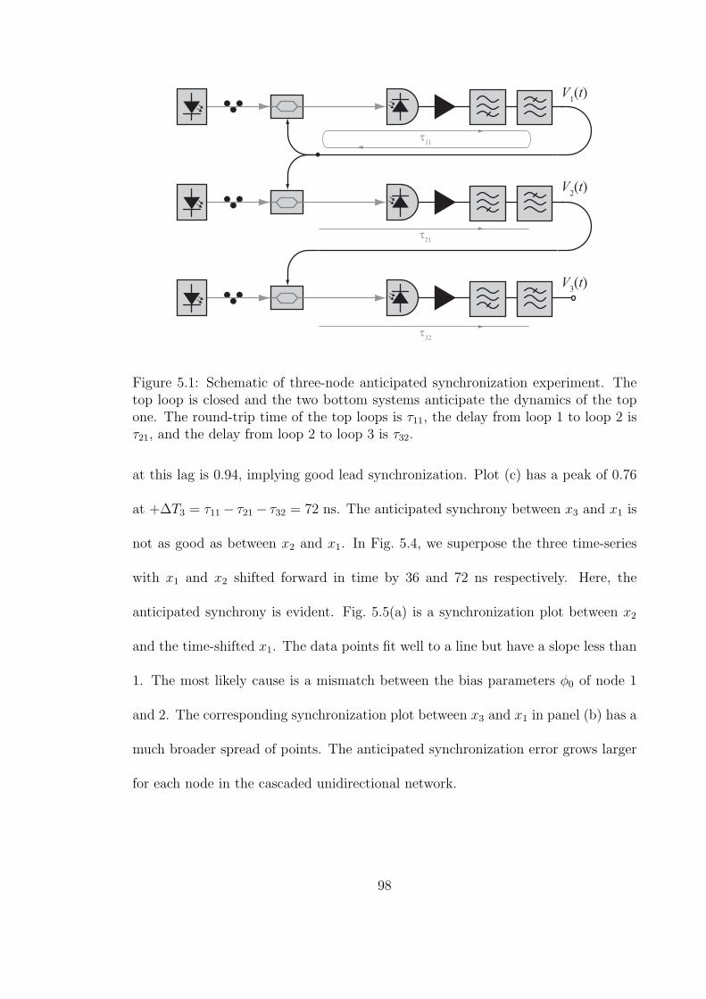
V1(t)

τ11

τ21

V2(t)

V3(t)

τ32

Figure 5.1: Schematic of three-node anticipated synchronization experiment. Thetop loop is closed and the two bottom systems anticipate the dynamics of the topone. The round-trip time of the top loops is τ11, the delay from loop 1 to loop 2 isτ21, and the delay from loop 2 to loop 3 is τ32.

at this lag is 0.94, implying good lead synchronization. Plot (c) has a peak of 0.76

at +∆T3 = τ11 − τ21 − τ32 = 72 ns. The anticipated synchrony between x3 and x1 is

not as good as between x2 and x1. In Fig. 5.4, we superpose the three time-series

with x1 and x2 shifted forward in time by 36 and 72 ns respectively. Here, the

anticipated synchrony is evident. Fig. 5.5(a) is a synchronization plot between x2

and the time-shifted x1. The data points fit well to a line but have a slope less than

1. The most likely cause is a mismatch between the bias parameters ϕ0 of node 1

and 2. The corresponding synchronization plot between x3 and x1 in panel (b) has a

much broader spread of points. The anticipated synchronization error grows larger

for each node in the cascaded unidirectional network.

98

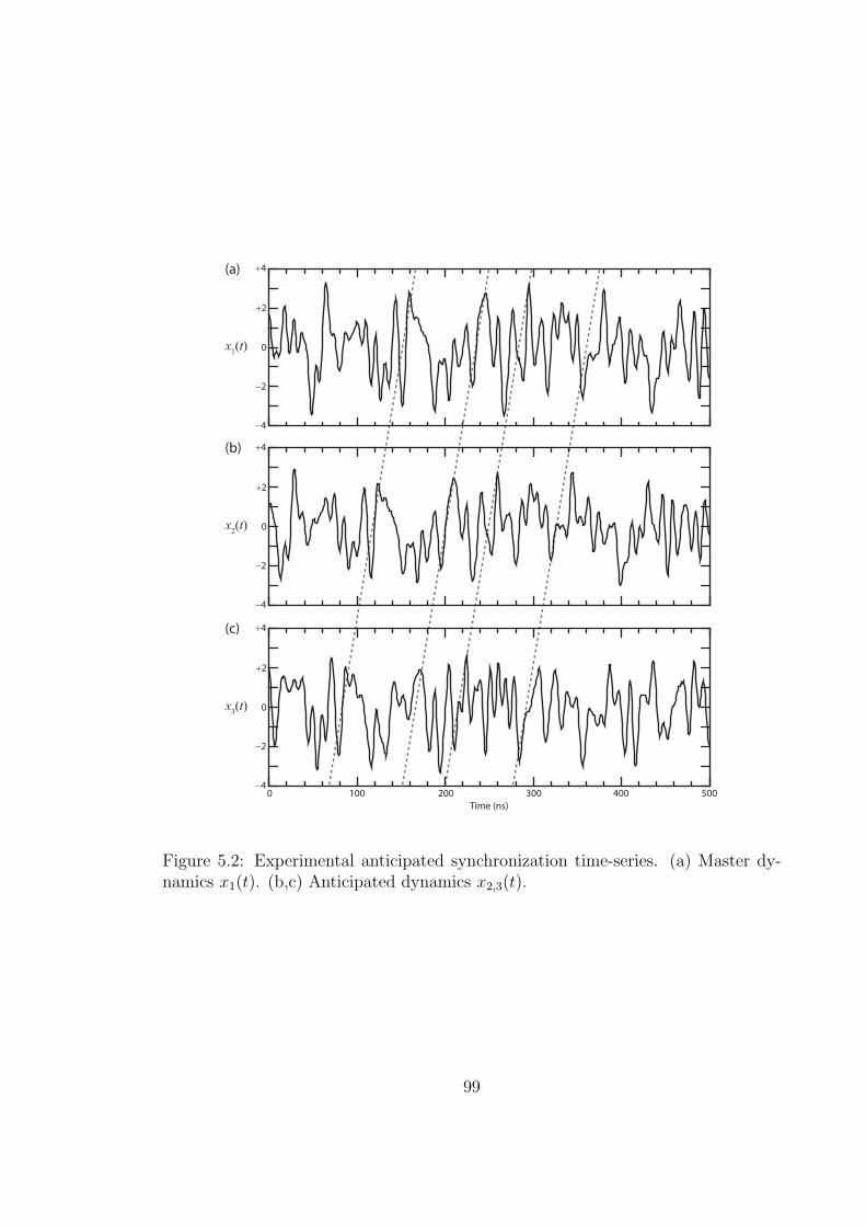
0x1(t)

−4

−2

+4

+2

0x2(t)

−4

−2

+4

+2

0

0 100 200

Time (ns)

300 400 500

x3(t)

−4

−2

+4

+2

(a)

(b)

(c)

Figure 5.2: Experimental anticipated synchronization time-series. (a) Master dy-namics x1(t). (b,c) Anticipated dynamics x2,3(t).

99

0

ρ11

0.2

−0.2

0.4

0.6

0.8

1.0

0

0.2

−0.2

0.4

0.6

0.8

1.0

0

0.2

−0.2

0.4

0.6

0.8

1.0

ρ12

−100−200 0

Time shift (ns)

100 200

ρ13

(a)

(b)

(c)

Figure 5.3: (a) Autocorrelation for x1. (b) Cross-correlation between x1 and x2

has a peak at ∆T = 36 ns. (c) Cross-correlation between x1 and x3 has a peak at2∆T = 72 ns.

0

0 100 200

Time (ns)

300 400 500−4

−2

+4

+2

x1(t+2∆T) x

2(t+∆T) x

3(t)

Figure 5.4: Time-shifted experimental time-series.

100

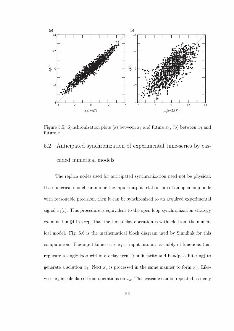
0

−4

−2

+4

+2

0−4 −2 +4+2

x1(t+∆T)

x2(t)

0

−4

−2

+4

+2

0−4 −2 +4+2

x1(t+2∆T)

x3(t)

(a) (b)

Figure 5.5: Synchronization plots (a) between x2 and future x1, (b) between x3 andfuture x1.

5.2 Anticipated synchronization of experimental time-series by cas-

caded numerical models

The replica nodes used for anticipated synchronization need not be physical.

If a numerical model can mimic the input–output relationship of an open loop node

with reasonable precision, then it can be synchronized to an acquired experimental

signal x1(t). This procedure is equivalent to the open loop synchronization strategy

examined in §4.1 except that the time-delay operation is withheld from the numer-

ical model. Fig. 5.6 is the mathematical block diagram used by Simulink for this

computation. The input time-series x1 is input into an assembly of functions that

replicate a single loop within a delay term (nonlinearity and bandpass filtering) to

generate a solution x2. Next x2 is processed in the same manner to form x3. Like-

wise, x4 is calculated from operations on x3. This cascade can be repeated as many

101

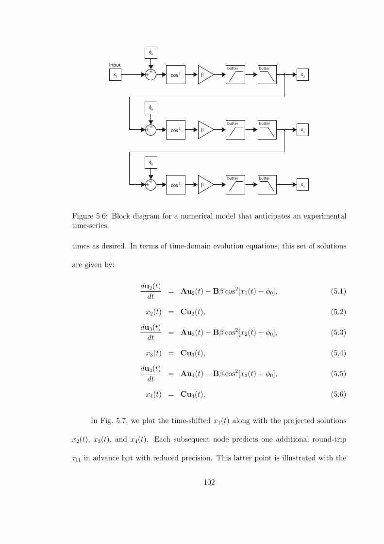
cos 2 β

φ0

butter butter

x2

++

x1

input

cos 2 β

φ0

butter butter

x3

++

cos 2 β

φ0

butter butter

x4

++

Figure 5.6: Block diagram for a numerical model that anticipates an experimentaltime-series.

times as desired. In terms of time-domain evolution equations, this set of solutions

are given by:

du2(t)

dt= Au2(t)−Bβ cos2[x1(t) + ϕ0], (5.1)

x2(t) = Cu2(t), (5.2)

du3(t)

dt= Au3(t)−Bβ cos2[x2(t) + ϕ0], (5.3)

x3(t) = Cu3(t), (5.4)

du4(t)

dt= Au4(t)−Bβ cos2[x3(t) + ϕ0], (5.5)

x4(t) = Cu4(t). (5.6)

In Fig. 5.7, we plot the time-shifted x1(t) along with the projected solutions

x2(t), x3(t), and x4(t). Each subsequent node predicts one additional round-trip

τ11 in advance but with reduced precision. This latter point is illustrated with the

102

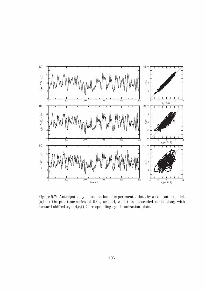
0

x1(t+∆T

), x

2(t

)x

1(t+

2∆T

), x

3(t

)x

1(t+

3∆T

), x

4(t

)

−4

−2

+4

+2

0

−4

−2

+4

+2

0

0 100 200

Time (ns)

300 400 500

0 100 200 300 400 500

0 100 200 300 400 500

−4

−2

+4

+2

0

0−4−4

−2

−2

+4

+4

+2

+2

0−4 −2 +4+2

0−4 −2 +4+2

0

−4

−2

+4

+2

0

−4

−2

+4

+2

(a)

(b)

(c)

(d)

(e)

(f )

x1(t+∆T)

x2(t

)x

3(t

)

x1(t+2∆T)

x1(t+3∆T)

x4(t

)

Figure 5.7: Anticipated synchronization of experimental data by a computer model.(a,b,c) Output time-series of first, second, and third cascaded node along withforward-shifted x1. (d,e,f) Corresponding synchronization plots.

103

synchronization plots (b), (d), and (f) which become systematically broader.

Anticipated synchronization can be used to extend the prediction technique

surveyed in Chapter 4 and Ref. [10]. The numerical model for an isolated op-

toelectronic feedback oscillator is relatively accurate, and it synchronizes to real

experimental data with high precision. The prediction horizon time can be length-

ened by using a series of cascaded numerical models rather than a single loop. At

a specified time t, the experimental input x1(t) can be terminated and replaced by

a delayed feedback term. The input to the first node x1(t) can be replaced with

x2(t − τ11). The cascaded series has more information about the history of the ex-

perimental system than a single loop, and may be able to make longer predictions

with confidence.

104

5.3 Summary

1. Synchrony of a network with time-delayed couplings may be achronal (lead

and lag) or isochronal (zero-lag).

2. Anticipated synchrony can occur for a unidirectional chain of oscillators, and

it is practically useful for time-series prediction.

3. A network of optoelectronic time-delay oscillators is a good testbed system for

experiments on anticipated synchronization.

4. We have experimentally demonstrated the phenomenon of anticipated syn-

chronization with two cascaded oscillators.

5. If a numerical model can precisely reproduce the chaotic behavior of an oscil-

lator, then it can be used for prediction by anticipated synchronization.

105

Chapter 6

Stability of adaptive synchronization1

An adaptive synchronization technique maintains synchrony on a network of

chaotic oscillators even when the coupling strengths Aij are a priori unknown and

time-varying in possibly an unpredictable manner. In Ref. [37], an adaptive strategy

was proposed in which each node in the network seeks to minimize a local measure

of synchronization error via gradient descent. Operationally, a control system at

each node manages the strength of the incoming signal ri by applying a multiplica-

tive weight. This weighting procedure ensures that a globally synchronous state is

admitted. The signal ri is assumed to be a linear superposition of the outputs of

all the nodes. In Ref. [37], the adaptive technique was numerically verified to syn-

chronize a network of low dimensional chaotic oscillators. In Ref. [5], the adaptive

technique was experimentally demonstrated on a network of two unidirectionally

coupled optoelectronic feedback loops with a fluctuating coupling strength A12(t).

For a channel modulation of the form A21(t) = A0 +∆A0 sin(2πFt), the quality of

synchronization was systematically tested as a function of the amplitude ∆A0 and

frequency F . In Ref. [42], a bidirectionally coupled three-node network of optoelec-

tronic loops was used to test the range of operation and applicability for sensing

and tracking changes to the coupling strengths.

A pertinent question is how the adaptive technique and its associated time-

1Portions of this Chapter are modified excerpts from Ref. [42].

106

scales modify the stability of the synchronous state. Investigations into this topic

are presented in Refs. [42] and [52] in which the master stability function formalism

[30] was extended to incorporate the adaptive rule. In this Chapter, we outline the

key results and apply them to a network of optoelectronic feedback loops. We also

quantify geometrical symmetries of the derived master stability function. Recent

results claim that the stability contours for a network of time-delay systems, for

which optoelectronic oscillators are an example, have a specific, well-defined shape

in the complex plane [55].

In §6.1, we review the adaptive synchronization strategy and presents its equa-

tions of motion and control as a discrete-time map. We apply the strategy to a

network of optoelectronic feedback loops with DSP-based filtering, time delay, and

control (see §2.11).

In §6.2, we derive the master stability function for the case of adaptive control

and we compute the stability contours for a network of optoelectronic nodes.

In §6.3, we introduce an experimental three-node network with symmetric cou-

pling strengths (A12 = A21, A23 = A32, A31 = A13) that can be adjusted arbitrarily

for Aij ≥ 0. We measure the range of stability for a given network configuration by

measuring the synchronization error as a single coupling parameter is tuned, and

we interpret the results based on the master stability function.

In §6.4, we consider numerical simulations on an adaptive network of N = 25

nodes and study the synchronous behavior for different control time-scales.

In §6.5, we review the main findings of Ref. [55] and quantify the rotational

symmetry of the specific master stability function with time-delayed couplings de-

107

rived here.

6.1 Review of adaptive synchronization strategy

Here we present the equations for an adaptive network in discrete time. Let

the state of node i = 1, . . . , N at time n be xi[n]. The coupled dynamics are the N

map equations:

xi[n] = F(xi[n− 1]) + εvN∑j=1

AijH(xj[n− 1]) (6.1)

where we assume a scalar output function H(x) which is added into the dynamics

with the vector v. We assume that node i only has access to the net coupling

signal ri =∑N

j=1AijH(xj) and its local counterpart H(xi) but not to each of the

summands AijH(xj) nor the individual matrix elements Aij. Only if the row sums

of the adjacency matrix A are uniform, i.e. ki ≡∑N

j=1 Aij = k0 for all i, is a globally

synchronous solution xi[n] = s[n] possible. If so, then the state

s[n] = F(s[n− 1]) + εvk0H(s[n− 1]) (6.2)

defines motion on the (N − 1)-dimensional synchronous manifold x1 = · · · = xN .

For network-based synchronization studies, it is often taken for granted that the row

sum condition is satisfied. However, for an arbitrarily chosen network configuration,

this is seldom case. Moreover, even if a network is initially tuned to have ki = k0 for

all i, the uniform row sums are not preserved when there are changes in the Aij’s

such as an interrupted coupling path (Aij → 0 for a specific i and j) or temporal

drift in coupling strengths (Aij → Aij[n]).

108

One method to enforce the possibility of synchrony is to have each node weight

the incoming net coupling term ri by ki. Then the effective coupling matrix is

A′ij = Aij/ki and the condition

∑Nj=1A

′ij = 1 is met by definition. (We assume

ki > 0 so that there are no problems with division by zero.) The adaptive technique

described here seeks to construct real-time estimates of the ki’s, even as they vary

in time: ki = ki[n]. Let ki be the estimate of ki. We reexpress Eqs. (6.1) as

xi[n] = F(xi[n− 1]) + εv1

ki[n− 1]

N∑j=1

AijH(xj[n− 1]) (6.3)

The update equations for ki[n] are derived and motivated in Refs. [5], [37], [42], and

[52], and they are:

1

ki[n]=

pi[n]

qi[n], (6.4)

pi[n] = z0pi[n− 1] + (1− z0)(ri[n]H(xi[n])), (6.5)

qi[n] = z0qi[n− 1] + (1− z0)(ri[n])2, (6.6)

where z0 is a parameter that determines the time-scales for which ki can successfully

track variations in the coupling strengths. Explicitly, z0 defines the smoothing factor

for an exponentially weighted moving average of (ri[n]H(xi[n])) and (ri[n])2 for pi

and qi respectively. The averaging window has a characteristic length of (1− z0)−1

samples or T = Ts(1 − z0)−1 where Ts is the interval between successive samples n

and n+ 1. The range of z0 is (0, 1) and a smaller value allowing for faster tracking

(corresponding to a shorter averaging time T ). However, as we describe in §6.2, the

ability to track a faster variation comes at the cost of a reduced synchronization

range.

109

In some situations, such an adaptive network can be designed to act as a sensor

network. As such, the set of estimated row sums ki[n] can be used to uniquely

resolve each of the individual coupling terms Aij[n] in real-time. For a symmetrically

coupled three-node network, it is possible to compute the three coupling strengths

Aij = Aji by algebraically solving the equations ki =∑3

j=1 Aij, i = 1, 2, 3. Thus, if a

centralized hub has access to k1[n], k2[n] and k3[n], then the complete time-varying

network topology A[n] can be ascertained.

We now outline how the adaptive synchronization technique is applied to a

network of optoelectronic feedback loop oscillators. The uncontrolled equations of

motion are a network-generalization of Eq. (2.23):

xi[n] = −a1xi[n−1]−a2xi[n−2]−b0β

N∑j=1

Aij(cos(xj[n−k]+ϕ0)−cos(xj[n−k−2]+ϕ0))

(6.7)

where xi[n] is the digital bandpass filter output of node i and −β cos2(xj[n−k]+ϕ0)

is the output by node j delayed by k time units. Eq. (6.7) can be cast in the

form of Eq. (6.1) by defining the state vectors xi[n] as a set of delay coordinates

incorporating the last (k+2) iterates. The adaptive strategy is operationally applied

by programming the DSP board installed at each node to solve for pi[n] and qi[n]

and to scale the feedback strength as: β → β/ki[n] = β(pi[n]/qi[n]). Here β plays

the role of ε in Eq. (6.1). The specific details regarding the order of operations as

implemented by the DSP and how to define F(x), H(x), and v in terms of Eqs.

(6.1) are presented in Ref. [42].

The adaptive strategy was implemented on a three-node network, as depicted

110

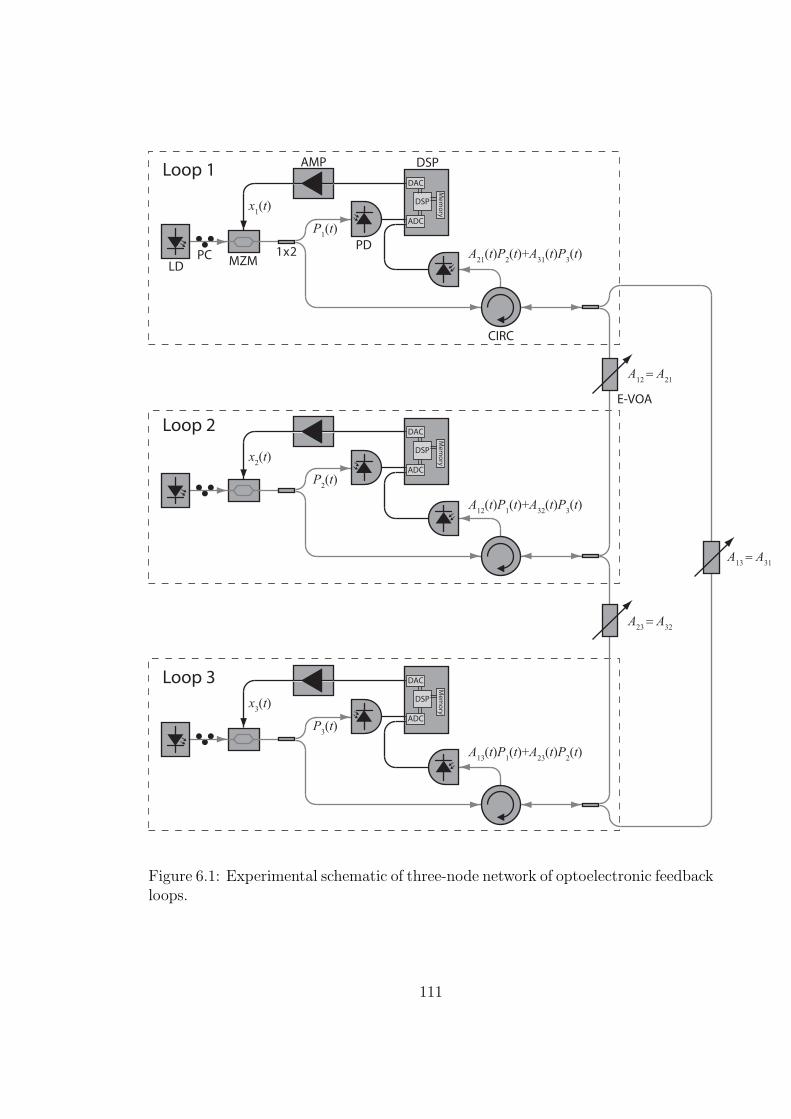
ADC

DAC

DSP

Memory

ADC

DAC

DSP

Memory

ADC

DAC

DSP

Memory

LDPC 1 x 2

PD

DSPAMP

Loop 2

Loop 1

Loop 3

CIRC

P1(t)

A21

(t)P2(t)+A

31(t)P

3(t)

A12

(t)P1(t)+A

32(t)P

3(t)

A13

(t)P1(t)+A

23(t)P

2(t)

A12

= A21

A23

= A32

A13

= A31

x1(t)

P2(t)

x2(t)

P3(t)

x3(t)

E-VOA

MZM

Figure 6.1: Experimental schematic of three-node network of optoelectronic feedbackloops.

111

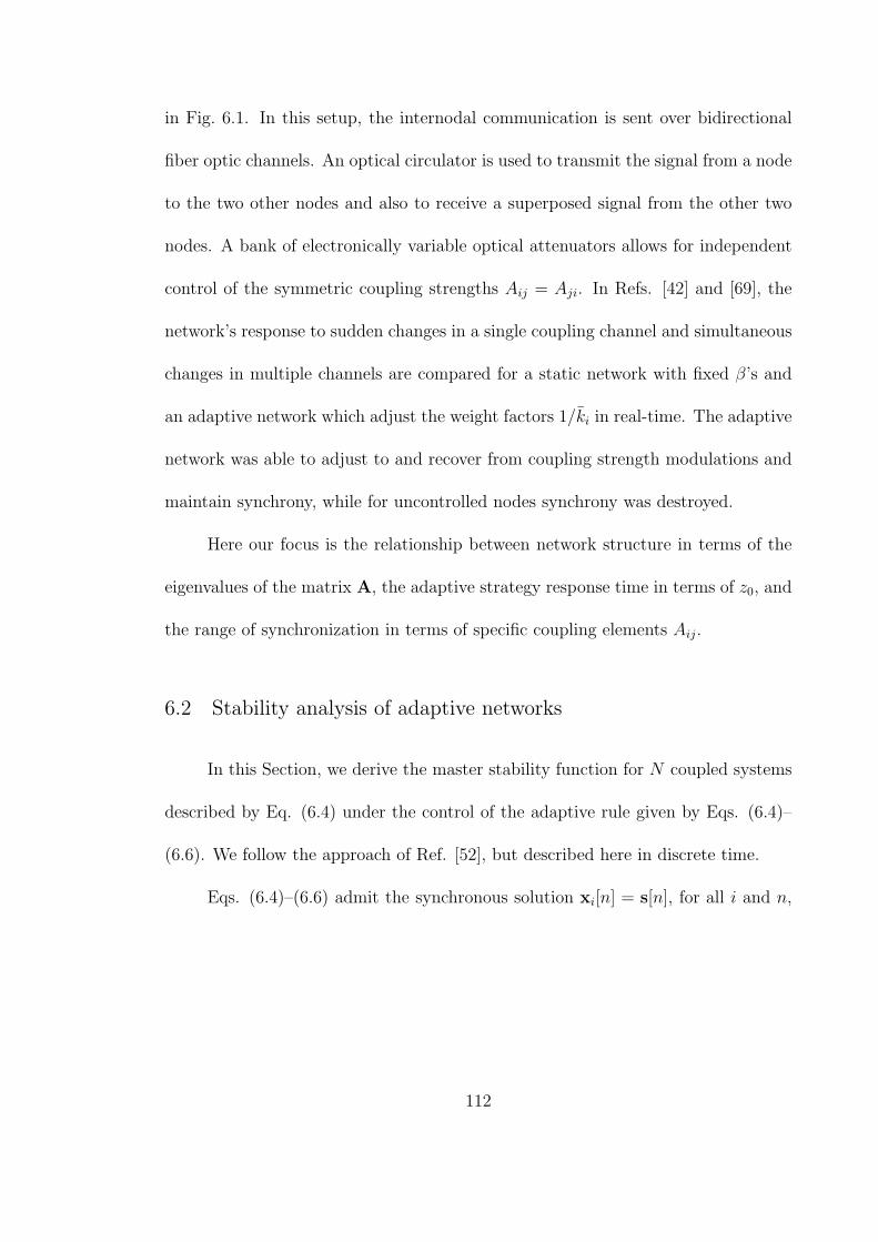
in Fig. 6.1. In this setup, the internodal communication is sent over bidirectional

fiber optic channels. An optical circulator is used to transmit the signal from a node

to the two other nodes and also to receive a superposed signal from the other two

nodes. A bank of electronically variable optical attenuators allows for independent

control of the symmetric coupling strengths Aij = Aji. In Refs. [42] and [69], the

network’s response to sudden changes in a single coupling channel and simultaneous

changes in multiple channels are compared for a static network with fixed β’s and

an adaptive network which adjust the weight factors 1/ki in real-time. The adaptive

network was able to adjust to and recover from coupling strength modulations and

maintain synchrony, while for uncontrolled nodes synchrony was destroyed.

Here our focus is the relationship between network structure in terms of the

eigenvalues of the matrix A, the adaptive strategy response time in terms of z0, and

the range of synchronization in terms of specific coupling elements Aij.

6.2 Stability analysis of adaptive networks

In this Section, we derive the master stability function for N coupled systems

described by Eq. (6.4) under the control of the adaptive rule given by Eqs. (6.4)–

(6.6). We follow the approach of Ref. [52], but described here in discrete time.

Eqs. (6.4)–(6.6) admit the synchronous solution xi[n] = s[n], for all i and n,

112

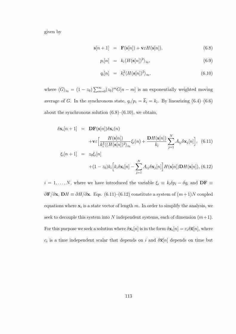
given by

s[n+ 1] = F(s[n]) + vεH(s[n]), (6.8)

pi[n] = ki⟨H(s[n])2⟩z0 , (6.9)

qi[n] = k2i ⟨H(s[n])2⟩z0 , (6.10)

where ⟨G⟩z0 = (1 − z0)∑∞

m=0(z0)mG[n − m] is an exponentially weighted moving

average of G. In the synchronous state, qi/pi = ki = ki. By linearizing (6.4)–(6.6)

about the synchronous solution (6.8)–(6.10), we obtain,

δxi[n+ 1] = DF(s[n])δxi(n)

+vε[ H(s[n])

k2i ⟨(H(s[n])2⟩z0

ξi(n) +DH(s[n])

ki

N∑j=1

Aijδxj[n]], (6.11)

ξi[n+ 1] = z0ξi[n]

+(1− z0)ki

[kiδxi[n]−

N∑j=1

Aijδxj[n]]H(s[n])DH(s[n]), (6.12)

i = 1, . . . , N , where we have introduced the variable ξi ≡ kiδpi − δqi and DF ≡

∂F/∂x, DH ≡ ∂H/∂x. Eqs. (6.11)–(6.12) constitute a system of (m+1)N coupled

equations where xi is a state vector of length m. In order to simplify the analysis, we

seek to decouple this system into N independent systems, each of dimension (m+1).

For this purpose we seek a solution where δxi[n] is in the form δxi[n] = ciδx[n], where

ci is a time independent scalar that depends on i and δx[n] depends on time but

113

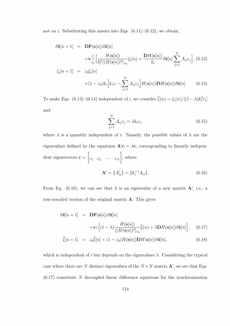
not on i. Substituting this ansatz into Eqs. (6.11)–(6.12), we obtain,

δx[n+ 1] = DF(s[n])δx[n]

+vε

ci

[ H(s[n])

k2i ⟨(H(s[n])2⟩z0

ξi(n) +DH(s[n])

kiδx[n]

N∑j=1

Aijcj

], (6.13)

ξi[n+ 1] = z0ξi[n]

+(1− z0)ki

[kici −

N∑j=1

Aijcj

]H(s[n])DH(s[n])δx[n]. (6.14)

To make Eqs. (6.13)–(6.14) independent of i, we consider ξ(n) = ξi(n)/[(1−λ)k2i ci]

andN∑j=1

Aijcj = λkici, (6.15)

where λ is a quantity independent of i. Namely, the possible values of λ are the

eigenvalues defined by the equatuon A′c = λc, corresponding to linearly indepen-

dent eigenvectors c =

[c1 c2 · · · cN

], where

A′ = A′ij = k−1

i Aij. (6.16)

From Eq. (6.16), we can see that λ is an eigenvalue of a new matrix A′, i.e., a

row-rescaled version of the original matrix A. This gives

δx[n+ 1] = DF(s[n])δx[n]

+vε[(1− λ)

H(s[n])

⟨(H(s[n])2⟩z0ξ(n) + λDH(s[n])δx[n]

], (6.17)

ξ[n+ 1] = z0ξ[n] + (1− z0)H(s[n])DH(s[n])δx[n], (6.18)

which is independent of i but depends on the eigenvalues λ. Considering the typical

case where there are N distinct eigenvalues of the N×N matrix A′, we see that Eqs.

(6.17) constitute N decoupled linear difference equations for the synchronization

114

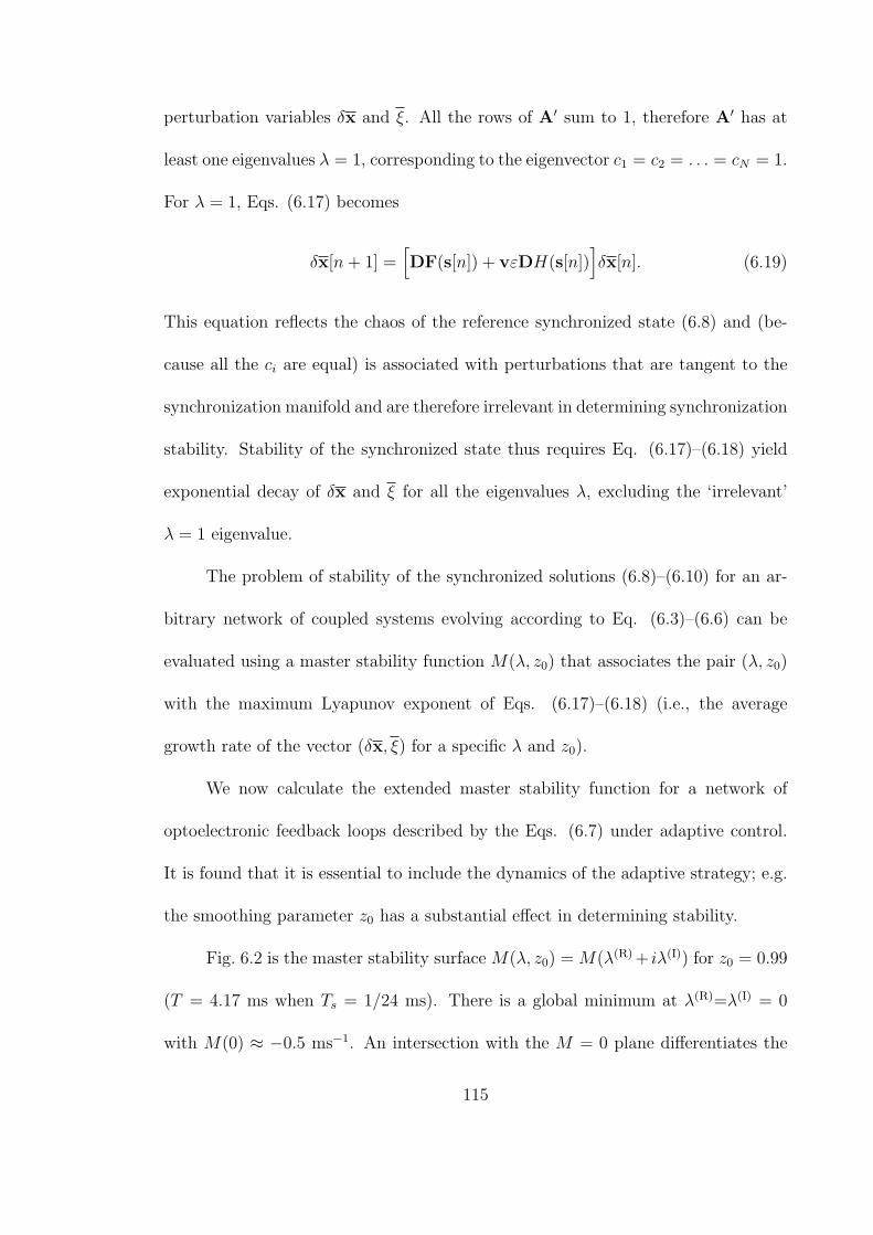
perturbation variables δx and ξ. All the rows of A′ sum to 1, therefore A′ has at

least one eigenvalues λ = 1, corresponding to the eigenvector c1 = c2 = . . . = cN = 1.

For λ = 1, Eqs. (6.17) becomes

δx[n+ 1] =[DF(s[n]) + vεDH(s[n])

]δx[n]. (6.19)

This equation reflects the chaos of the reference synchronized state (6.8) and (be-

cause all the ci are equal) is associated with perturbations that are tangent to the

synchronization manifold and are therefore irrelevant in determining synchronization

stability. Stability of the synchronized state thus requires Eq. (6.17)–(6.18) yield

exponential decay of δx and ξ for all the eigenvalues λ, excluding the ‘irrelevant’

λ = 1 eigenvalue.

The problem of stability of the synchronized solutions (6.8)–(6.10) for an ar-

bitrary network of coupled systems evolving according to Eq. (6.3)–(6.6) can be

evaluated using a master stability function M(λ, z0) that associates the pair (λ, z0)

with the maximum Lyapunov exponent of Eqs. (6.17)–(6.18) (i.e., the average

growth rate of the vector (δx, ξ) for a specific λ and z0).

We now calculate the extended master stability function for a network of

optoelectronic feedback loops described by the Eqs. (6.7) under adaptive control.

It is found that it is essential to include the dynamics of the adaptive strategy; e.g.

the smoothing parameter z0 has a substantial effect in determining stability.

Fig. 6.2 is the master stability surface M(λ, z0) = M(λ(R)+ iλ(I)) for z0 = 0.99

(T = 4.17 ms when Ts = 1/24 ms). There is a global minimum at λ(R)=λ(I) = 0

with M(0) ≈ −0.5 ms−1. An intersection with the M = 0 plane differentiates the

115

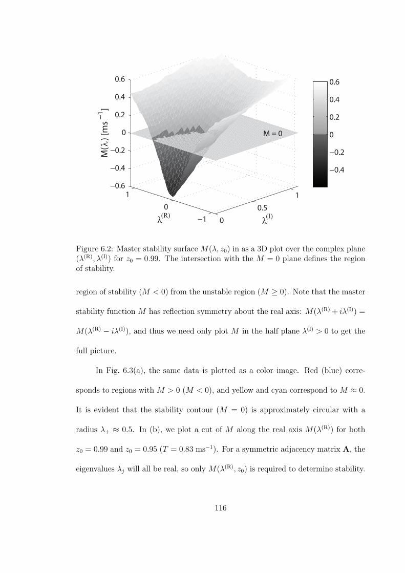
0

0.5

1

−1

0

1

−0.6

−0.4

−0.2

0

0.2

0.4

0.6

λ(I)

λ(R)

M(λ) [ms−1]

−0.4

−0.2

0

0.2

0.4

0.6

M = 0

Figure 6.2: Master stability surface M(λ, z0) in as a 3D plot over the complex plane(λ(R), λ(I)) for z0 = 0.99. The intersection with the M = 0 plane defines the regionof stability.

region of stability (M < 0) from the unstable region (M ≥ 0). Note that the master

stability function M has reflection symmetry about the real axis: M(λ(R) + iλ(I)) =

M(λ(R) − iλ(I)), and thus we need only plot M in the half plane λ(I) > 0 to get the

full picture.

In Fig. 6.3(a), the same data is plotted as a color image. Red (blue) corre-

sponds to regions with M > 0 (M < 0), and yellow and cyan correspond to M ≈ 0.

It is evident that the stability contour (M = 0) is approximately circular with a

radius λ+ ≈ 0.5. In (b), we plot a cut of M along the real axis M(λ(R)) for both

z0 = 0.99 and z0 = 0.95 (T = 0.83 ms−1). For a symmetric adjacency matrix A, the

eigenvalues λj will all be real, so only M(λ(R), z0) is required to determine stability.

116

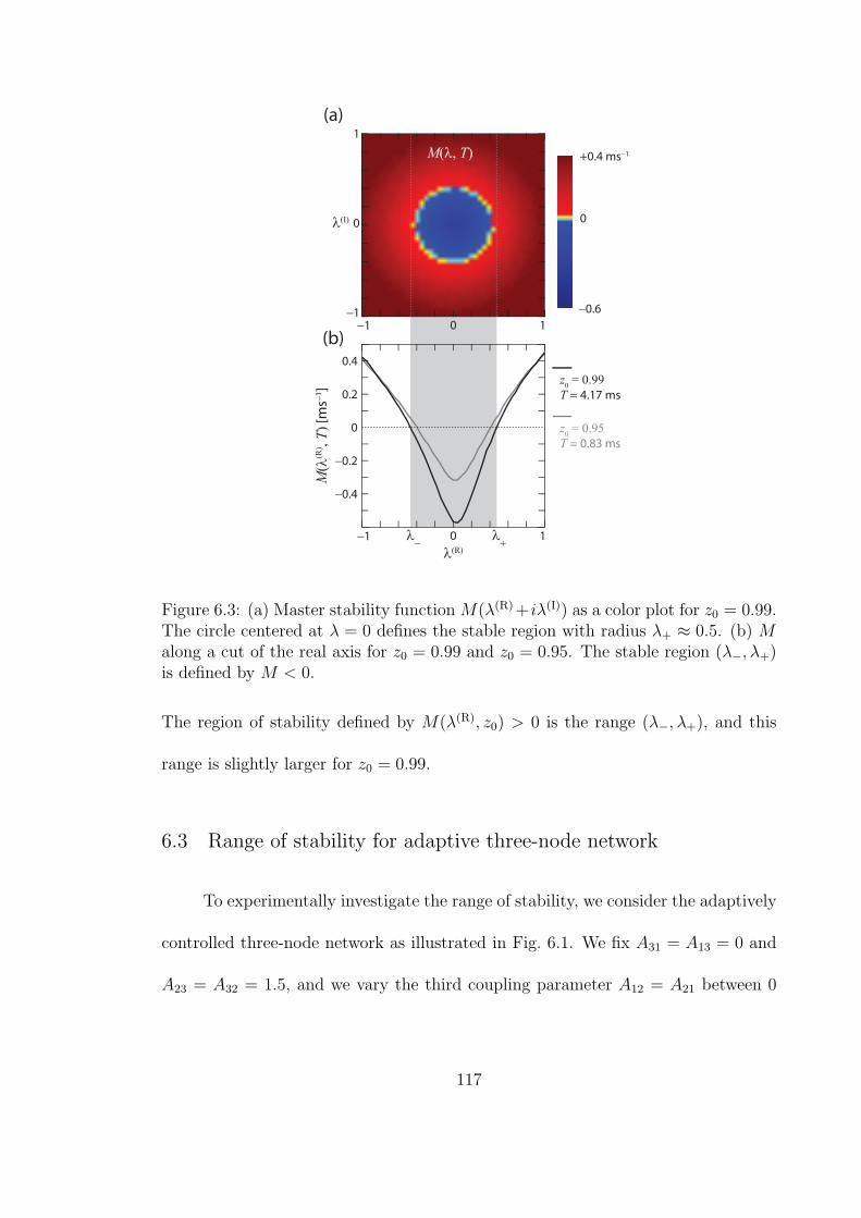
−1 0

λ(R)

M(λ

(R) ,

T)

[ms−

1]

(a)

(b)

M(λ, T)

λ−

λ+

0

−0.2

−0.4

0.2

0.4

1

λ(I)

−1

−0.6−1

0

00

1

+0.4 ms−1

1

z0 = 0.99

T = 4.17 ms

z0 = 0.95

T = 0.83 ms

Figure 6.3: (a) Master stability function M(λ(R)+ iλ(I)) as a color plot for z0 = 0.99.The circle centered at λ = 0 defines the stable region with radius λ+ ≈ 0.5. (b) Malong a cut of the real axis for z0 = 0.99 and z0 = 0.95. The stable region (λ−, λ+)is defined by M < 0.

The region of stability defined by M(λ(R), z0) > 0 is the range (λ−, λ+), and this

range is slightly larger for z0 = 0.99.

6.3 Range of stability for adaptive three-node network

To experimentally investigate the range of stability, we consider the adaptively

controlled three-node network as illustrated in Fig. 6.1. We fix A31 = A13 = 0 and

A23 = A32 = 1.5, and we vary the third coupling parameter A12 = A21 between 0

117

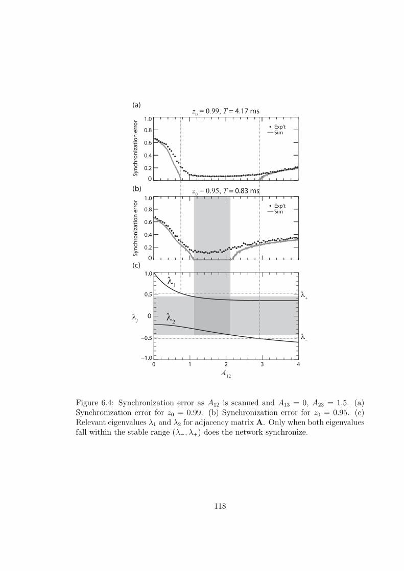
0−1.0

−0.5

0

0

0.2

0.4

0.6

0.8

1.0

0.5

1.0

1 432

A12

λj

λ+

λ−

λ2

λ1

0

0.2

0.4

0.6

0.8

1.0

Sy

nc

hro

niz

ati

on

err

or

Sy

nc

hro

niz

ati

on

err

or

z0 = 0.99, T = 4.17 ms

z0 = 0.95, T = 0.83 ms

Exp’tSim

Exp’tSim

(a)

(b)

(c)

Figure 6.4: Synchronization error as A12 is scanned and A13 = 0, A23 = 1.5. (a)Synchronization error for z0 = 0.99. (b) Synchronization error for z0 = 0.95. (c)Relevant eigenvalues λ1 and λ2 for adjacency matrix A. Only when both eigenvaluesfall within the stable range (λ−, λ+) does the network synchronize.

118

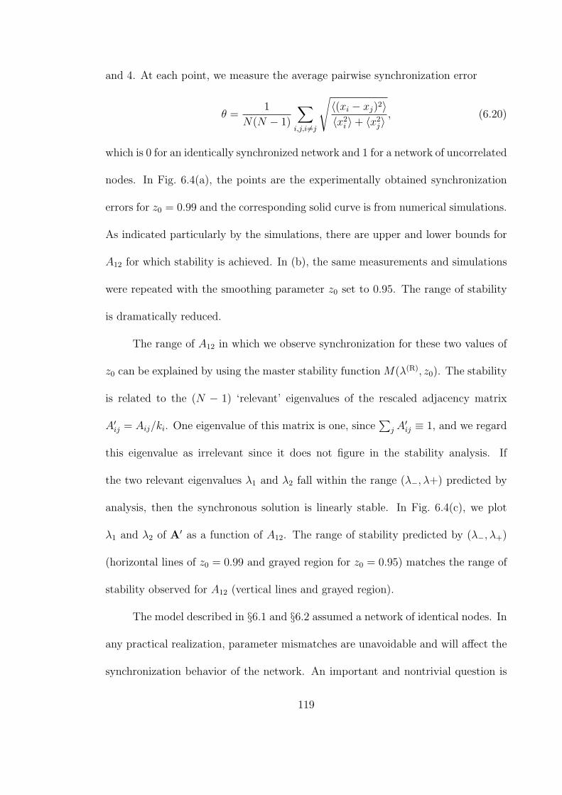
and 4. At each point, we measure the average pairwise synchronization error

θ =1

N(N − 1)

∑i,j,i =j

√⟨(xi − xj)2⟩⟨x2

i ⟩+ ⟨x2j⟩

, (6.20)

which is 0 for an identically synchronized network and 1 for a network of uncorrelated

nodes. In Fig. 6.4(a), the points are the experimentally obtained synchronization

errors for z0 = 0.99 and the corresponding solid curve is from numerical simulations.

As indicated particularly by the simulations, there are upper and lower bounds for

A12 for which stability is achieved. In (b), the same measurements and simulations

were repeated with the smoothing parameter z0 set to 0.95. The range of stability

is dramatically reduced.

The range of A12 in which we observe synchronization for these two values of

z0 can be explained by using the master stability function M(λ(R), z0). The stability

is related to the (N − 1) ‘relevant’ eigenvalues of the rescaled adjacency matrix

A′ij = Aij/ki. One eigenvalue of this matrix is one, since

∑j A

′ij ≡ 1, and we regard

this eigenvalue as irrelevant since it does not figure in the stability analysis. If

the two relevant eigenvalues λ1 and λ2 fall within the range (λ−, λ+) predicted by

analysis, then the synchronous solution is linearly stable. In Fig. 6.4(c), we plot

λ1 and λ2 of A′ as a function of A12. The range of stability predicted by (λ−, λ+)

(horizontal lines of z0 = 0.99 and grayed region for z0 = 0.95) matches the range of

stability observed for A12 (vertical lines and grayed region).

The model described in §6.1 and §6.2 assumed a network of identical nodes. In

any practical realization, parameter mismatches are unavoidable and will affect the

synchronization behavior of the network. An important and nontrivial question is

119

how well the adaptive strategy works when there are small deviations from identical-

ity of the nodes. Here, we find good agreement between our theoretical calculation

which assumes identical nodes and experiments where there is some parameter tol-

erance. We conclude that the theory, as presented, is applicable for making realistic

predictions about which actual networks will synchronize. Moreover, our stability

theory, based on the master stability function formalism, can be extended to the

case of mismatches in a network of nearly identical systems [104, 105, 106].

6.4 Numerical experiments of a 25-node network

As a further example, we numerically consider a network of optoelectronic

systems in which we have a relatively large number of nodes (N = 25) and in which

the couplings are directional; i.e. Aij may differ from Aji. For cases with A not

symmetric the eigenvalues of A′ may be complex. The two contours in Fig. 6.5 (a)

and (c) indicate the region of the complex plane within which the eigenvalues of

A′ must fall in order to maintain synchrony, i.e., the region for which the master

stability function, M(λ, z0) is negative. The contours were obtained with z0 = 0.99

and z0 = 0.95. When constructing the adjacency matrix, we randomly choose each

of the Aij to be either 1/7 or 0, with probability 0.25 and 0.75, respectively; the

diagonal elements Aii are 1/7. This choice of adjacency matrix yields a distribution

of row sums for which the adaptive algorithm must compensate. The eigenvalues

of A′ are plotted in the complex planes in Fig. 6.5 (a) and (c). The (N − 1)

relevant eigenvalues fall within the region for stable synchrony when z0 = 0.99 (a)

120

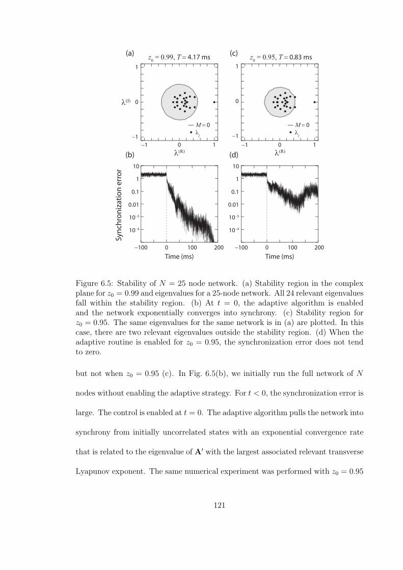
λ(I)

λ(R) λ(R)

Sy

nch

ron

iza

tio

n e

rro

r

(a)

(b)

(c)

(d)

−1

−1

0

0 100

10

1

0.1

0.01

10−3

10−4

10

1

0.1

0.01

10−3

10−4

200−100 0 100 200−100

0

M = 0

z0 = 0.99, T = 4.17 ms z

0 = 0.95, T = 0.83 ms

λj

1

1

−1

−1

0

0

M = 0

λj

1

1

Time (ms) Time (ms)

Figure 6.5: Stability of N = 25 node network. (a) Stability region in the complexplane for z0 = 0.99 and eigenvalues for a 25-node network. All 24 relevant eigenvaluesfall within the stability region. (b) At t = 0, the adaptive algorithm is enabledand the network exponentially converges into synchrony. (c) Stability region forz0 = 0.95. The same eigenvalues for the same network is in (a) are plotted. In thiscase, there are two relevant eigenvalues outside the stability region. (d) When theadaptive routine is enabled for z0 = 0.95, the synchronization error does not tendto zero.

but not when z0 = 0.95 (c). In Fig. 6.5(b), we initially run the full network of N

nodes without enabling the adaptive strategy. For t < 0, the synchronization error is

large. The control is enabled at t = 0. The adaptive algorithm pulls the network into

synchrony from initially uncorrelated states with an exponential convergence rate

that is related to the eigenvalue of A′ with the largest associated relevant transverse

Lyapunov exponent. The same numerical experiment was performed with z0 = 0.95

121

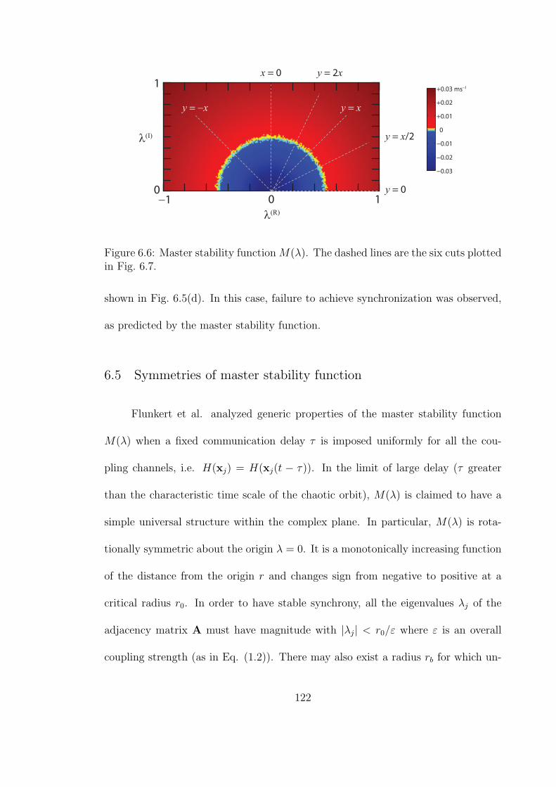
λ(R)

λ(I)

−1 00

1

1

y = 0

y = x/2

y = x

y = 2xx = 0

y = −x

−0.03

+0.03 ms−1

−0.02

−0.01

0

+0.01

+0.02

Figure 6.6: Master stability functionM(λ). The dashed lines are the six cuts plottedin Fig. 6.7.

shown in Fig. 6.5(d). In this case, failure to achieve synchronization was observed,

as predicted by the master stability function.

6.5 Symmetries of master stability function

Flunkert et al. analyzed generic properties of the master stability function

M(λ) when a fixed communication delay τ is imposed uniformly for all the cou-

pling channels, i.e. H(xj) = H(xj(t − τ)). In the limit of large delay (τ greater

than the characteristic time scale of the chaotic orbit), M(λ) is claimed to have a

simple universal structure within the complex plane. In particular, M(λ) is rota-

tionally symmetric about the origin λ = 0. It is a monotonically increasing function

of the distance from the origin r and changes sign from negative to positive at a

critical radius r0. In order to have stable synchrony, all the eigenvalues λj of the

adjacency matrix A must have magnitude with |λj| < r0/ε where ε is an overall

coupling strength (as in Eq. (1.2)). There may also exist a radius rb for which un-

122

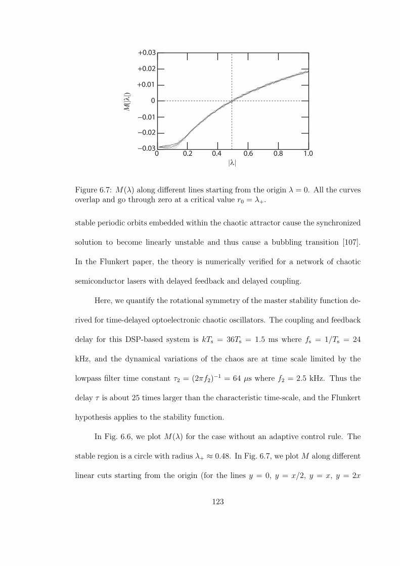
0 0.2 0.4

|λ|

M(|λ|)

0.6 0.8 1.0−0.03

+0.03

−0.02

−0.01

+0.01

0

+0.02

Figure 6.7: M(λ) along different lines starting from the origin λ = 0. All the curvesoverlap and go through zero at a critical value r0 = λ+.

stable periodic orbits embedded within the chaotic attractor cause the synchronized

solution to become linearly unstable and thus cause a bubbling transition [107].

In the Flunkert paper, the theory is numerically verified for a network of chaotic

semiconductor lasers with delayed feedback and delayed coupling.

Here, we quantify the rotational symmetry of the master stability function de-

rived for time-delayed optoelectronic chaotic oscillators. The coupling and feedback

delay for this DSP-based system is kTs = 36Ts = 1.5 ms where fs = 1/Ts = 24

kHz, and the dynamical variations of the chaos are at time scale limited by the

lowpass filter time constant τ2 = (2πf2)−1 = 64 µs where f2 = 2.5 kHz. Thus the

delay τ is about 25 times larger than the characteristic time-scale, and the Flunkert

hypothesis applies to the stability function.

In Fig. 6.6, we plot M(λ) for the case without an adaptive control rule. The

stable region is a circle with radius λ+ ≈ 0.48. In Fig. 6.7, we plot M along different

linear cuts starting from the origin (for the lines y = 0, y = x/2, y = x, y = 2x

123

−0.8−0.8

0.4

−0.4

0

λ(R)

M(λ, T) = 0

λ(I) 0

0.4

4

8

128

0.4

0.8

0.8

Figure 6.8: Stability contours M(λ, z0) = 0 for different values of z0. The sixcontours are for z0 such that the averaging window (1− z0)

−1 is 4, 8, 16, 32, 64, and128 time steps. For shorter averaging times, the rotational symmetry is broken.

and y = −x where λ = x+ iy, as depicted by dashed lines in Fig. 6.6). All of these

curves fall roughly on top of one another; thus M is indeed rotationally symmetric.

To further examine the shape for time-delayed master stability functions, we

calculate the stability contours M = 0 as we vary the adaptive control time-scale

coefficient z0. We expect that as z0 → 0 the region of stability shrinks and as z0 → 1

the region asymptotically approaches the uncontrolled case. In Fig. 6.8, the contours

for (1−z0)−1 = 4, 8, 16, 32, 64, and 128 are plotted. For the latter four examples, the

shape closely resembles a circle. For the 4 and 8 cases, where the region of stability

is focused closely near λ = 0, the circular symmetry is broken. The adaptive control

algorithm introduces a new time scale for the dynamical behavior T = Ts(1− z0)−1

in terms of the state variables pi and qi. For small T , the time scale of the coupled

system (xi, pi, qi) may be dominated by T rather than τL, and thus the Flunkert

124

0

0 40 80 120 160 200

2Averaging window T (ms)

Averaging window (samples)

Sta

bil

ity

ra

diu

s λ

+

0

0.1

0.2

0.3

0.4

0.5

4 6 8

Figure 6.9: Stability radius of as averaging time T = Ts(1 − z0)−1 is varied. For

T > 2 ms, they asymptotically approach r0 ≈ 0.45.

theory fails. In Fig. 6.9, we plot the critical radius r0 of the master stability function

M as a function of the adaption coefficient T . The radius asymptotically approaches

an upper bound. This result is practically useful in choosing the z0 parameter that

maximizes the range of stability for a given speed of channel fluctuations. It is

evident that choosing T much larger than 2 ms has little effect on enlarging the

range of stable operation.

For a rotationally symmetric master stability function, all the information

about the stability of the synchronous state for an arbitrary weighted network is

composed in single scalar function M(|λ|). Only the magnitudes of the relevant

eigenvalues |λj| are required to determine if the configuration A can maintain syn-

chronous operation. A two-node unidirectional network with a variable coupling

strength A21 can be used to ascertain the stability range. Namely by determining

the upper and lower bound of A12 for which the two oscillators synchronize, the

stability radius r0 is ascertained and can be applied to all configurations of N oscil-

125

lators. This is a powerful result that reduces the complexity of the stability problem

for a large class of time-delay networks.

126

6.6 Summary

1. An adaptive synchronization scheme maintains the synchronous state of identi-

cal coupled chaotic oscillators in the presence of time-varying coupling strengths.

2. The stability of adaptive synchronization is addressed by extending the master

stability function technique to include adaptation.

3. The eigenvalues of the rescaled coupling matrix A′ must fall within a specified

region of the complex plane for the network to support synchronism.

4. The range of stability is substantially affected by the adaptation coefficient

which characterizes the time-scales for which an adaptive network can sense

perturbations to its coupling structure.

5. The master stability function for the class of time-delay networks has a circular

shape in the complex plane.

127

Chapter 7

Prediction of network convergence rate

Upon enabling coupling and information exchange, the dynamics of an initially

noninteracting collection of chaotic oscillators may fall into a state of synchronism.

The master stability function framework allows us to predict whether a given inter-

action arrangement fosters such entrainment [30]. Recently, the rate µ at which a

synchronizable network converges into synchrony has been recognized as an impor-

tant metric for classifying and ranking the network [56]. A faster convergence rate

is correlated with enhanced stability, more rapid recovery from perturbations, and

reduced sensitivity to parameter mismatches and noise. These observations can also

be understood in terms of the master stability function framework, which mathe-

matically decouples the detailed time evolution of each node on the network from

the dynamical role performed by the network interaction structure. While network

structure underlies the process of synchronization, we can analyze network struc-

ture independently from the dynamics on the network . In particular, experiments

on a small network (in which all the system parameters are under precise control)

can be used to infer or predict the performance of much larger networks [58]. In

this chapter, we study the convergence properties of a two-node auxiliary network,

develop a theory of how to apply the results to an arbitrary network, and test the

conjecture with experiments on a four-node network and numerical simulations of a

128

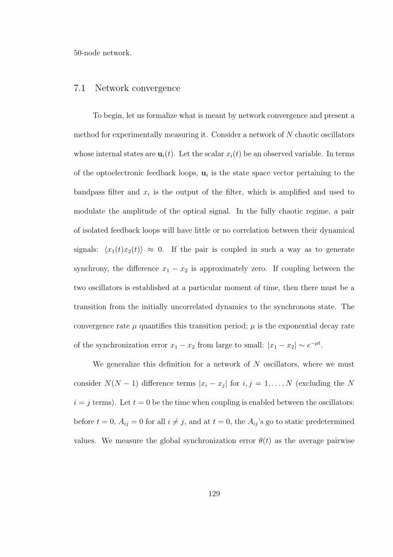
50-node network.

7.1 Network convergence

To begin, let us formalize what is meant by network convergence and present a

method for experimentally measuring it. Consider a network of N chaotic oscillators

whose internal states are ui(t). Let the scalar xi(t) be an observed variable. In terms

of the optoelectronic feedback loops, ui is the state space vector pertaining to the

bandpass filter and xi is the output of the filter, which is amplified and used to

modulate the amplitude of the optical signal. In the fully chaotic regime, a pair

of isolated feedback loops will have little or no correlation between their dynamical

signals: ⟨x1(t)x2(t)⟩ ≈ 0. If the pair is coupled in such a way as to generate

synchrony, the difference x1 − x2 is approximately zero. If coupling between the

two oscillators is established at a particular moment of time, then there must be a

transition from the initially uncorrelated dynamics to the synchronous state. The

convergence rate µ quantifies this transition period; µ is the exponential decay rate

of the synchronization error x1 − x2 from large to small: |x1 − x2| ∼ e−µt.

We generalize this definition for a network of N oscillators, where we must

consider N(N − 1) difference terms |xi − xj| for i, j = 1, . . . , N (excluding the N

i = j terms). Let t = 0 be the time when coupling is enabled between the oscillators:

before t = 0, Aij = 0 for all i = j, and at t = 0, the Aij’s go to static predetermined

values. We measure the global synchronization error θ(t) as the average pairwise

129

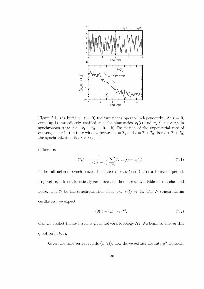
(a)

(b)

−2

4

2

0

−2

−4

−1 0 1 2

Time (ms)

Time (ms)

To

T+To

x1(t) x

2(t)

0 4 8 12−4

1

0.1

0.01

|x1(t

) – x

2(t

)| slope ∼ −µ

Figure 7.1: (a) Initially (t < 0) the two nodes operate independently. At t = 0,coupling is immediately enabled and the time-series x1(t) and x2(t) converge insynchronous state, i.e. x1 − x2 → 0. (b) Estimation of the exponential rate ofconvergence µ in the time window between t = T0 and t = T + T0. For t > T + T0,the synchronization floor is reached.

difference:

θ(t) =1

N(N − 1)

∑i,j=1

N |xi(t)− xj(t)|. (7.1)

If the full network synchronizes, then we expect θ(t) ≈ 0 after a transient period.

In practice, it is not identically zero, because there are unavoidable mismatches and

noise. Let θ0 be the synchronization floor, i.e. θ(t) → θ0. For N synchronizing

oscillators, we expect

(θ(t)− θ0) ∼ e−µt. (7.2)

Can we predict the rate µ for a given network topology A? We begin to answer this

question in §7.5.

Given the time-series records xi(t), how do we extract the rate µ? Consider

130

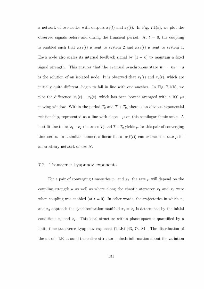
a network of two nodes with outputs x1(t) and x2(t). In Fig. 7.1(a), we plot the

observed signals before and during the transient period. At t = 0, the coupling

is enabled such that κx1(t) is sent to system 2 and κx2(t) is sent to system 1.

Each node also scales its internal feedback signal by (1 − κ) to maintain a fixed

signal strength. This ensures that the eventual synchronous state u1 = u2 = s

is the solution of an isolated node. It is observed that x1(t) and x2(t), which are

initially quite different, begin to fall in line with one another. In Fig. 7.1(b), we

plot the difference |x1(t) − x2(t)| which has been boxcar averaged with a 100 µs

moving window. Within the period T0 and T + T0, there is an obvious exponential

relationship, represented as a line with slope −µ on this semilogarithmic scale. A

best fit line to ln⟨|x1−x2|⟩ between T0 and T +T0 yields µ for this pair of converging

time-series. In a similar manner, a linear fit to ln⟨θ(t)⟩ can extract the rate µ for

an arbitrary network of size N .

7.2 Transverse Lyapunov exponents

For a pair of converging time-series x1 and x2, the rate µ will depend on the

coupling strength κ as well as where along the chaotic attractor x1 and x2 were

when coupling was enabled (at t = 0). In other words, the trajectories in which x1

and x2 approach the synchronization manifold x1 = x2 is determined by the initial

conditions x1 and x2. This local structure within phase space is quantified by a

finite time transverse Lyapunov exponent (TLE) [43, 73, 84]. The distribution of

the set of TLEs around the entire attractor embeds information about the variation

131

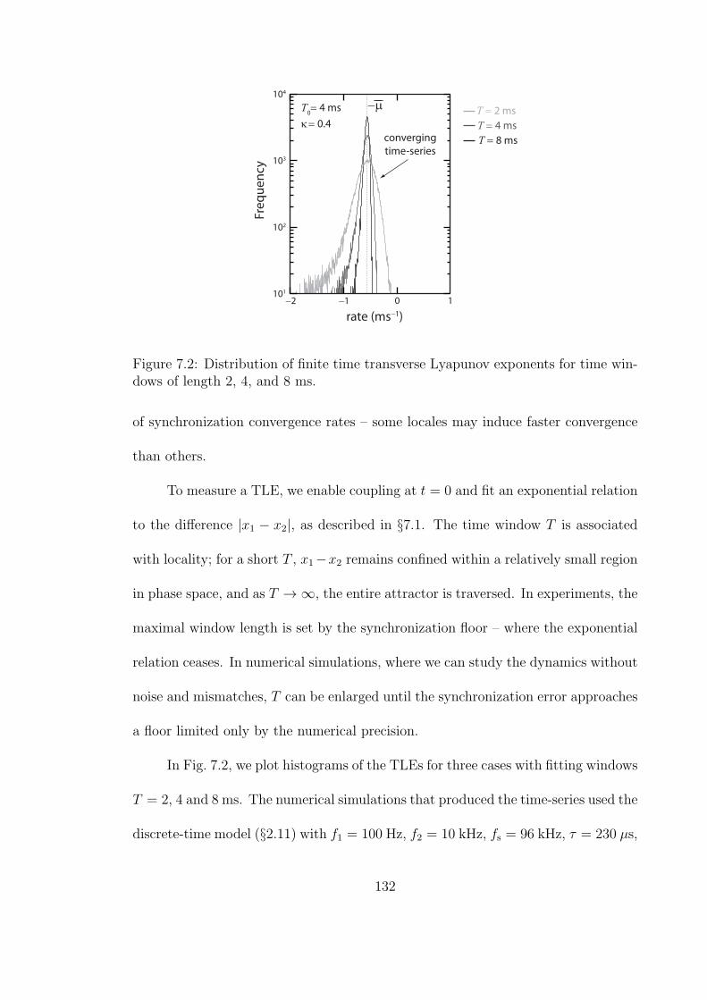
−2

104

103

102

101

−1 0 1

rate (ms−1)

Fre

qu

en

cy

T0= 4 ms

κ = 0.4

−µ

T = 8 msconverging

time-series

T = 4 ms

T = 2 ms

Figure 7.2: Distribution of finite time transverse Lyapunov exponents for time win-dows of length 2, 4, and 8 ms.

of synchronization convergence rates – some locales may induce faster convergence

than others.

To measure a TLE, we enable coupling at t = 0 and fit an exponential relation

to the difference |x1 − x2|, as described in §7.1. The time window T is associated

with locality; for a short T , x1−x2 remains confined within a relatively small region

in phase space, and as T → ∞, the entire attractor is traversed. In experiments, the

maximal window length is set by the synchronization floor – where the exponential

relation ceases. In numerical simulations, where we can study the dynamics without

noise and mismatches, T can be enlarged until the synchronization error approaches

a floor limited only by the numerical precision.

In Fig. 7.2, we plot histograms of the TLEs for three cases with fitting windows

T = 2, 4 and 8 ms. The numerical simulations that produced the time-series used the

discrete-time model (§2.11) with f1 = 100 Hz, f2 = 10 kHz, fs = 96 kHz, τ = 230 µs,

132

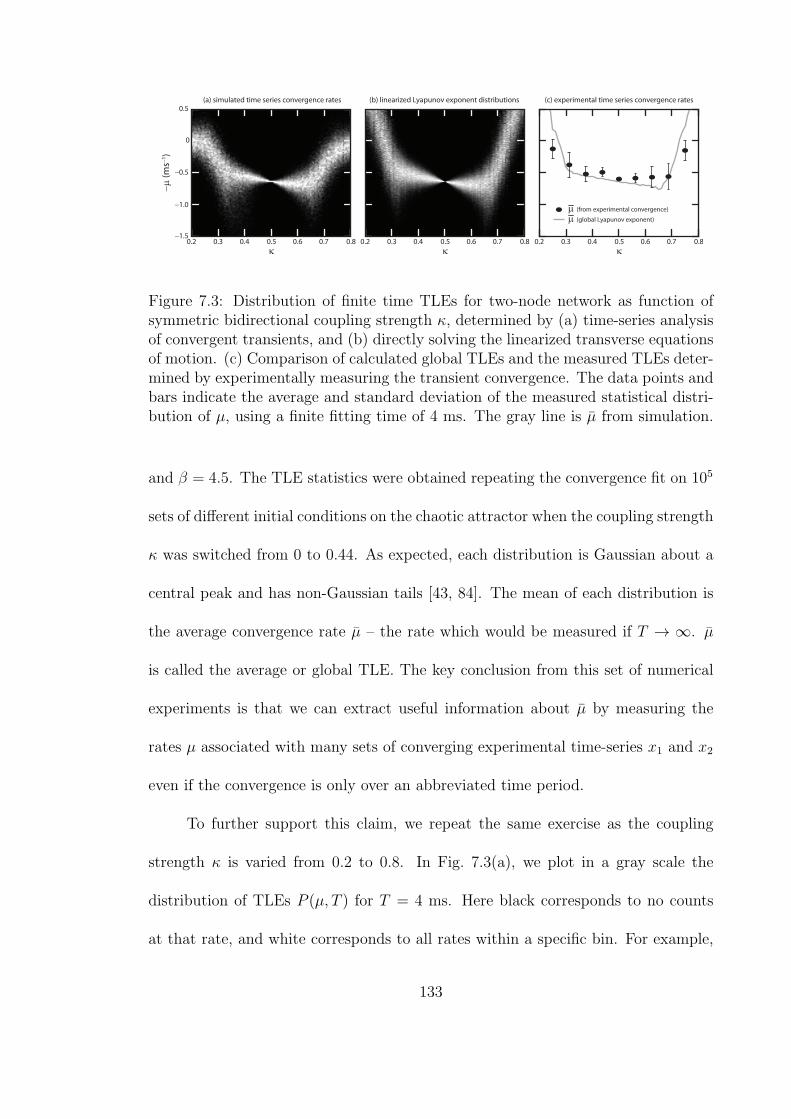
0.2

−0.5

−1.0

−1.5

0.5

0

0.3

(a) simulated time series convergence rates (b) linearized Lyapunov exponent distributions (c) experimental time series convergence rates

0.4 0.5

κ

−µ

(m

s−1)

µ (from experimental convergence)

0.6 0.7 0.8 0.2 0.3 0.4 0.5

κ0.6 0.7 0.8 0.2 0.3 0.4 0.5

κ0.6 0.7 0.8

µ (global Lyapunov exponent)

Figure 7.3: Distribution of finite time TLEs for two-node network as function ofsymmetric bidirectional coupling strength κ, determined by (a) time-series analysisof convergent transients, and (b) directly solving the linearized transverse equationsof motion. (c) Comparison of calculated global TLEs and the measured TLEs deter-mined by experimentally measuring the transient convergence. The data points andbars indicate the average and standard deviation of the measured statistical distri-bution of µ, using a finite fitting time of 4 ms. The gray line is µ from simulation.

and β = 4.5. The TLE statistics were obtained repeating the convergence fit on 105

sets of different initial conditions on the chaotic attractor when the coupling strength

κ was switched from 0 to 0.44. As expected, each distribution is Gaussian about a

central peak and has non-Gaussian tails [43, 84]. The mean of each distribution is

the average convergence rate µ – the rate which would be measured if T → ∞. µ

is called the average or global TLE. The key conclusion from this set of numerical

experiments is that we can extract useful information about µ by measuring the

rates µ associated with many sets of converging experimental time-series x1 and x2

even if the convergence is only over an abbreviated time period.

To further support this claim, we repeat the same exercise as the coupling

strength κ is varied from 0.2 to 0.8. In Fig. 7.3(a), we plot in a gray scale the

distribution of TLEs P (µ, T ) for T = 4 ms. Here black corresponds to no counts

at that rate, and white corresponds to all rates within a specific bin. For example,

133

at κ = 0.5, x1 and x2 converge unconditionally at a rate determined only by the

bandpass filter response, so the distribution collapses to a delta function. At κ =

0.32 and κ = 0.68, the distributions are at their broadest – implying that there is a

wide variability in the observed rates µ. Since the µ’s are extracted from converging

time-series, only for κ values which allow stable synchrony do we obtain a reliable

measure. If (x1 − x2) 9 0, then the rate is not well-defined for this routine.

For Fig. 7.3(c), the same procedure was repeated, except for x1 and x2 obtained

from a series of experiments. The data points are the distribution mean µ for nine

values of κ and the vertical bars are the widths of the statistical distribution. The

statistics are for 100 independent trials for each coupling strength. The solid curve

is the asymptotic TLE obtained by numerically integrating a linearized model (the

subject of the next paragraph). Because of the excellent agreement between the

means and widths of (a) and (c), we conclude that this switch experiment is a

powerful tool for learning about network convergence properties. In particular, if

we observe the set of N time-series xi for an N node network while simultaneously

turning on all of the couplings, we can measure µ by calculating θ(t) as in Eq. (7.1)

above.

Finally, we compare the convergence rate µ obtained from analyzing transient

dynamics with the conventional technique of computing phase space expansion or

contraction via a linearized numerical model [30, 51]. We compute the growth rates

by linearizing the difference δu = u1 − u2 about the synchronous solution u1 =

u2 = s. We collect the growth factors αj, following the standard MLE procedure

(as outlined in §3.2.1). To obtain a finite time distribution of the µ’s, we perform

134

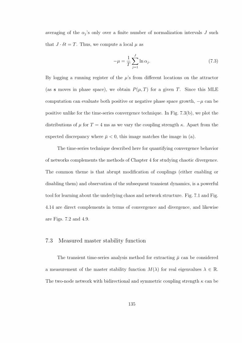
averaging of the αj’s only over a finite number of normalization intervals J such

that J · δt = T . Thus, we compute a local µ as

−µ =1

T

J∑j=1

lnαj. (7.3)

By logging a running register of the µ’s from different locations on the attractor

(as s moves in phase space), we obtain P (µ, T ) for a given T . Since this MLE

computation can evaluate both positive or negative phase space growth, −µ can be

positive unlike for the time-series convergence technique. In Fig. 7.3(b), we plot the

distributions of µ for T = 4 ms as we vary the coupling strength κ. Apart from the

expected discrepancy where µ < 0, this image matches the image in (a).

The time-series technique described here for quantifying convergence behavior

of networks complements the methods of Chapter 4 for studying chaotic divergence.

The common theme is that abrupt modification of couplings (either enabling or

disabling them) and observation of the subsequent transient dynamics, is a powerful

tool for learning about the underlying chaos and network structure. Fig. 7.1 and Fig.

4.14 are direct complements in terms of convergence and divergence, and likewise

are Figs. 7.2 and 4.9.

7.3 Measured master stability function

The transient time-series analysis method for extracting µ can be considered

a measurement of the master stability function M(λ) for real eigenvalues λ ∈ R.

The two-node network with bidirectional and symmetric coupling strength κ can be

135

cast into the form of a general network:

dxi

dt= F(xi) + ε

N∑j=1

AijH(xj) (7.4)

by setting N = 2 and

A =

1− κ κ

κ 1− κ

. (7.5)

The associated Laplacian matrix is

L =

κ −κ

−κ κ

(7.6)

which has eigenvalues λ1 = 0 and λ2 = 2κ. Since the two-node network has only a

single free eigenvalue 2κ, we may associate the convergence rate µ with the stability

function as −µ = M(λ = 2κ). However, unlike the standard routine for calculating

M(λ) from linearized equations, only negative values of M can be ascertained. This

does not limit the applicability of M(λ) since the rates yielded by master stability

function are only useful for synchronizable networks with M(λk) < 0. To establish

the range of λ = 2κ where µ = M(λ) is valid, we constrain the function to the

region with θ0 < 0.1, i.e. where the measured synchronization floor is reasonably

small.

In Fig. 7.4(a), we plot θ0 as function of λ for two optoelectronic feedback loops

with parameters f1 = 100 Hz, f2 = 2.5 kHz, fs = 24 kHz, τ = 1.5 ms, and β = 3.8.

The associated convergence rates M(λ) are plotted in (b). The grayed interval is the

region where M(λ) is trusted. The stable region along the real line is (0.57, 1.43).

To determine if a network will synchronize only θ0(λ) is required. For ex-

ample, for an arbitrary network with only real eigenvalues, all the eigenvalues λk

136

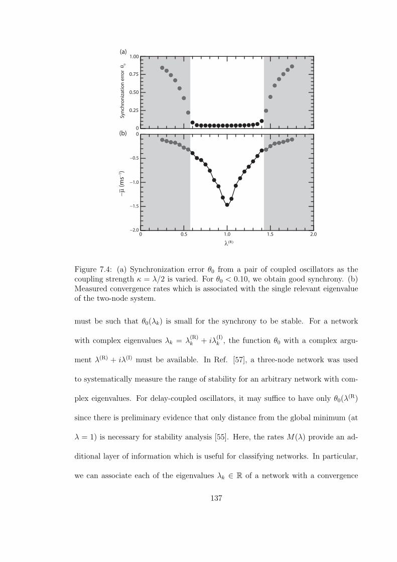
0

0

1.00

0

0.25

0.50

0.75

−0.5

−1.0

−1.5

−2.00.5 1.0

λ(R)

−µ

(m

s−1)

Sy

nch

ron

iza

tio

n e

rro

r θ0

(a)

(b)

1.5 2.0

Figure 7.4: (a) Synchronization error θ0 from a pair of coupled oscillators as thecoupling strength κ = λ/2 is varied. For θ0 < 0.10, we obtain good synchrony. (b)Measured convergence rates which is associated with the single relevant eigenvalueof the two-node system.

must be such that θ0(λk) is small for the synchrony to be stable. For a network

with complex eigenvalues λk = λ(R)k + iλ

(I)k , the function θ0 with a complex argu-

ment λ(R) + iλ(I) must be available. In Ref. [57], a three-node network was used

to systematically measure the range of stability for an arbitrary network with com-

plex eigenvalues. For delay-coupled oscillators, it may suffice to have only θ0(λ(R)

since there is preliminary evidence that only distance from the global minimum (at

λ = 1) is necessary for stability analysis [55]. Here, the rates M(λ) provide an ad-

ditional layer of information which is useful for classifying networks. In particular,

we can associate each of the eigenvalues λk ∈ R of a network with a convergence

137

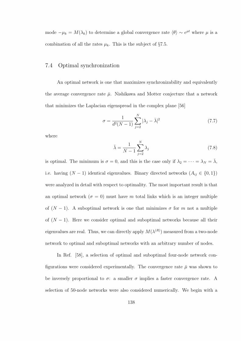
mode −µk = M(λk) to determine a global convergence rate ⟨θ⟩ ∼ eµt where µ is a

combination of all the rates µk. This is the subject of §7.5.

7.4 Optimal synchronization

An optimal network is one that maximizes synchronizability and equivalently

the average convergence rate µ. Nishikawa and Motter conjecture that a network

that minimizes the Laplacian eigenspread in the complex plane [56]

σ =1

d2(N − 1)

N∑j=2

|λj − λ|2 (7.7)

where

λ =1

N − 1

N∑j=2

λj (7.8)

is optimal. The minimum is σ = 0, and this is the case only if λ2 = · · · = λN = λ,

i.e. having (N − 1) identical eigenvalues. Binary directed networks (Aij ∈ 0, 1)

were analyzed in detail with respect to optimality. The most important result is that

an optimal network (σ = 0) must have m total links which is an integer multiple

of (N − 1). A suboptimal network is one that minimizes σ for m not a multiple

of (N − 1). Here we consider optimal and suboptimal networks because all their

eigenvalues are real. Thus, we can directly applyM(λ(R)) measured from a two-node

network to optimal and suboptimal networks with an arbitrary number of nodes.

In Ref. [58], a selection of optimal and suboptimal four-node network con-

figurations were considered experimentally. The convergence rate µ was shown to

be inversely proportional to σ: a smaller σ implies a faster convergence rate. A

selection of 50-node networks were also considered numerically. We begin with a

138

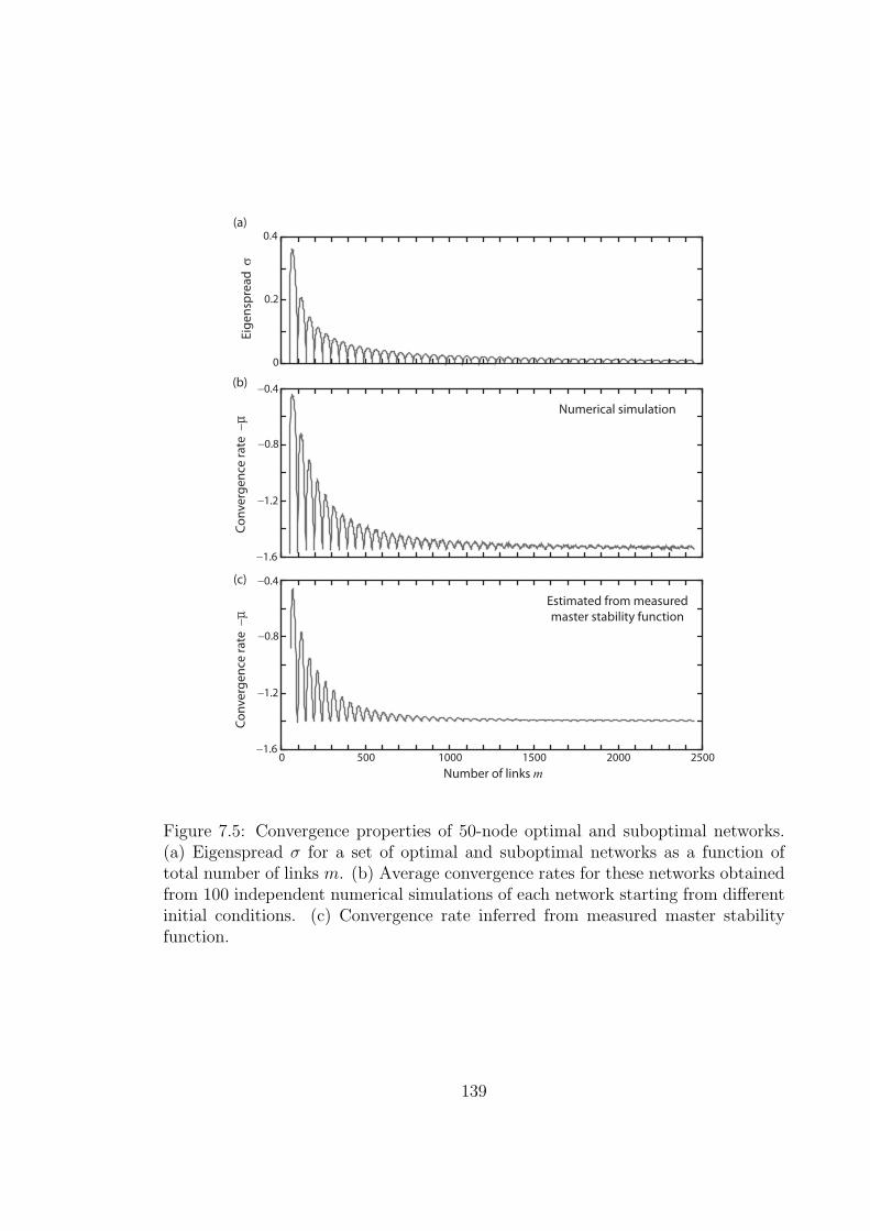
0 1000

Number of links m

Numerical simulation

(a)

(b)

(c)

Estimated from measured

master stability function

Eig

en

spre

ad

σC

on

ve

rge

nce

ra

te −µ

1500 2000 2500500

0.2

0

−0.4

0.4

−0.8

−1.2

−1.6

−0.4

−0.8

−1.2

−1.6

Co

nv

erg

en

ce r

ate

−µ

Figure 7.5: Convergence properties of 50-node optimal and suboptimal networks.(a) Eigenspread σ for a set of optimal and suboptimal networks as a function oftotal number of links m. (b) Average convergence rates for these networks obtainedfrom 100 independent numerical simulations of each network starting from differentinitial conditions. (c) Convergence rate inferred from measured master stabilityfunction.

139

fully connected network with m = N(N − 1) = 2450 links. This all-to-all network

is optimal with λk = λ for k = 2, . . . , N . Next, a link is removed as to keep σ mini-

mized. This process is repeated until only (N − 1) = 49 links remain. For the 2401

configurations considered, the Laplacian eigenvalue spectrum of each is populated

with only real numbers, even though many of the networks are asymmetric [56]. In

Fig. 7.5(a), we plot σ as a function of m, which follows a cusp-like path with minima

at m = (N − 1), 2(N − 1), . . . , N(N − 1) = 49, 98, . . . , 2450. In (b), we plot the

average convergence rate µ obtained from running a full nonlinear simulation for

each network. For each configuration, the abrupt coupling procedure was repeated

100 times, the synchronization error θ(t) was fit to an exponential relation, and the

average convergence rate µ is an average from all 100 trials. As expected from the-

ory, µ follows a cusp-like curve with m. Is there a way to predict µ without running

a full simulation, but instead utilizing the master stability function M(λ)?

7.5 Estimating convergence rate from master stability function

Each Laplacian eigenvalue λk is associated with a Lyapunov exponent M(λk).

Typically the function M(λ) is calculated via a linearized auxiliary equation. A

subject of this thesis (Chapters 4 and 7) is diagnosing the rates M(λk) via experi-

mental measurements. In §7.3, we measure M(λ) using controlled experiments on a

two-node network. In this section, we derive a formula for constructing the transient

rate µ from the rates −µk = M(λk).

It is often assumed that a network will converge at the slowest rate of the

140

set µkNk=2. However, this is only true infinitesimally close to the synchroniza-

tion manifold where excitations of all the other modes have decayed. Far from the

synchronization floor, the only regime available in experiments with a finite syn-

chronization floor, the influence along all eigendirections is important. Yet, it is

possible to use −µk = M(λk) to infer the expected transient rate. As described in

§7.4, this rate is important for real-world characterization of network optimality. In

general, we note that far from the synchronization manifold, the behavior may be

dominated by nonlinear terms that are excluded in the linear stability analysis.

Consider an N node network with (N − 1) relevant eigenvalues λk ∈ R. The

associated convergence eigenrates are −µk = M(λk) < 0. We expect each mode to

relax exponentially as e−µkt, such that the overall convergence takes the form

θ(t) ∼N∑k=2

Cke−µkt. (7.9)

The coefficients Ck are determined by the initial states of all the chaotic trajectories

u1,u2, . . . ,uN . However, if we repeat the measurement of θ(t) many times, we may

assume there is no preferential mode selected, and we set Ck = 1 for all k. We

assume ⟨θ(t)⟩ ∼ e−µt, then

e−µt =N∑k=2

e−µkt (7.10)

(where ⟨•⟩ represents an ensemble average over different choices of initial conditions).

Differentiating both sides of Eq. (7.10) with respect to t and solving for µ = µ(t),

we have:

µ(t) =

∑Nk=2 µke

−µkt∑Nk=2 e

−µkt. (7.11)

Thus, the observed convergence behavior µ is a time-varying combination of all the

141

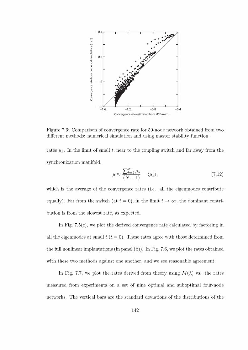
−0.4

−0.8

−1.2

−1.6−0.4−0.8−1.2

Co

nv

erg

en

ce r

ate

fro

m n

um

eri

cal s

imu

lati

on

s (m

s−1)

Convergence rate estimated from MSF (ms−1)

−1.6

Figure 7.6: Comparison of convergence rate for 50-node network obtained from twodifferent methods: numerical simulation and using master stability function.

rates µk. In the limit of small t, near to the coupling switch and far away from the

synchronization manifold,

µ ≈∑N

k=2 µk

(N − 1)= ⟨µk⟩, (7.12)

which is the average of the convergence rates (i.e. all the eigenmodes contribute

equally). Far from the switch (at t = 0), in the limit t → ∞, the dominant contri-

bution is from the slowest rate, as expected.

In Fig. 7.5(c), we plot the derived convergence rate calculated by factoring in

all the eigenmodes at small t (t = 0). These rates agree with those determined from

the full nonlinear implantations (in panel (b)). In Fig. 7.6, we plot the rates obtained

with these two methods against one another, and we see reasonable agreement.

In Fig. 7.7, we plot the rates derived from theory using M(λ) vs. the rates

measured from experiments on a set of nine optimal and suboptimal four-node

networks. The vertical bars are the standard deviations of the distributions of the

142

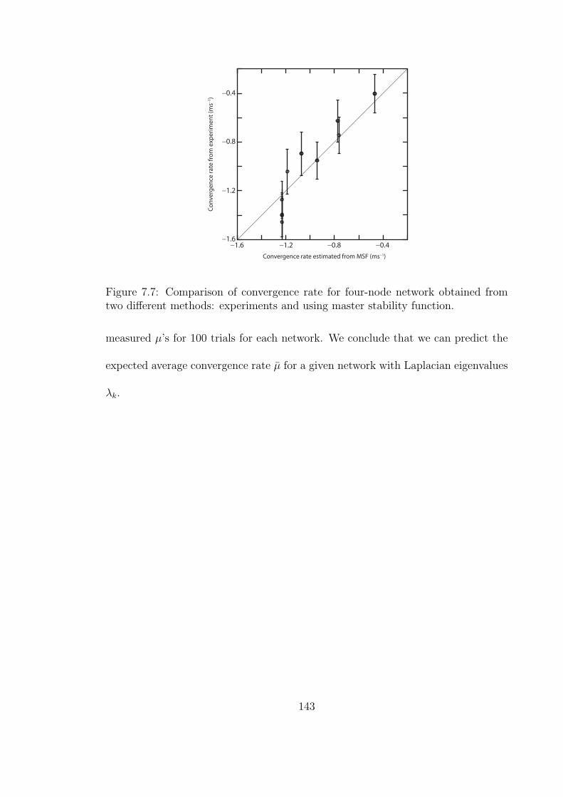
−0.4

−0.8

−1.2

−1.6−0.4−0.8−1.2

Co

nv

erg

en

ce r

ate

fro

m e

xpe

rim

en

t (m

s−1)

Convergence rate estimated from MSF (ms−1)

−1.6

Figure 7.7: Comparison of convergence rate for four-node network obtained fromtwo different methods: experiments and using master stability function.

measured µ’s for 100 trials for each network. We conclude that we can predict the

expected average convergence rate µ for a given network with Laplacian eigenvalues

λk.

143

7.6 Summary

1. The convergence rate to the synchronous state quantifies stability of a network.

2. We can measure convergence rates experimentally by enabling coupling be-

tween nodes and observing the transient dynamics to a synchronization floor.

3. The master stability function is used to predict the convergence rate for an

N -node network by incorporating all (N − 1) synchronization modes.

4. A two-node network with controllable coupling strengths is used to experi-

mentally measure the master stability function.

5. Optimal networks, which have (N − 1) identical Laplacian eigenvalues, have

the fastest rates of convergence.

144

Chapter 8

Conclusion

The major theme of the projects outlined in this thesis is that advances in

nonlinear science are achieved through a balance of controlled experiments, numer-

ical modeling, and theoretical analysis. In nonlinear systems, the dynamics of an

interconnected network cannot necessarily be understood in terms of the behav-

ior of the individual components. However, sometimes we can arrange a complex

network into a particular configuration that allows us to comprehend the myriad

interdependencies present in the system and identify the responsible mechanisms.

The phenomenon of synchronization – in which global order emerges out of a de-

centralized communication process – provides a powerful toolbox for studying and

applying chaos. The mathematical and experimental realizations of synchrony are

relatively simple, and yet they have provided fundamental insights into the nature

chaos and order. In this thesis, we focus on a prototype nonlinear oscillator which

captures many basic features found in a large class of systems, including: a route

into chaos, time-delayed feedback, and a range of time scales. We construct an array

of such node systems into a network, and we tune the network into synchrony. Ex-

perimentation and analysis of the synchronous state allows us to design a strategy

for time-series prediction and quantification of chaos, test an adaptive technique

for maintaining synchrony when coupling parameters fluctuate, and diagnose what

145

set of interactions optimize synchrony. While these procedures were applied to a

specific network of optoelectronic oscillators, the results have implications for our

basic understanding of other complex networks, including those composed of genes,

cells, or people. The main conclusion from the set of experiments, simulations, and

analyses presented in this thesis is: by observing the response of an entire network

to time-evolution of the network structure (be it slow variations in the individual

coupling strengths or rapid shocks that either induce or destroy synchrony), we can

garner a basic understanding of how collective behavior emerges.

8.1 Proposed research topics

In this final section, we discuss some ideas for potential topics of research on

a network of time-delayed optoelectronic feedback loops.

8.1.1 Random number generation

The chaos generated by a time-delayed feedback oscillator may be a source for

high-quality, difficult-to-predict pseudorandom numbers [7]. For example, the out-

put dynamical signal from a semiconductor laser with time-delayed optical feedback

has been shown to have no detectable non-random features by passing a battery of

statistical tests developed by NIST [7, 62, 77]. The optoelectronic feedback loops

hold promise as a random number generator. By increasing the bandwidth of the

feedback channel into tens of gigahertz, it is possible to sample the dynamical signal

with a high-speed digitizer. The output bit sequence can be analyzed for correlation

146

and patterns that are expected for chaotic motion. A major advantage of studying

optoelectronic feedback loops over other systems for this purpose is the potential

for realistic modeling of the underlying dynamics. For this system, the relationship

between randomness, dynamical entropy, and Lyapunov exponents can be studied

in detail. As parameters are tuned (such as delay, bandwidth, feedback strength,

and modulator bias), the complexity of the output bit sequences are also modified

in a predictable manner. Can dynamical complexity be associated with metrics for

quantifying randomness? For example, it may be that rare events embedded within

a chaotic attractor are responsible for amplification of stochastic noise and thus act

like a seed to sporadically reset the dynamics. Can this source of unpredictability

be described in terms of the non-Gaussian tail of distributions of local Lyapunov

exponents? The optoelectronic feedback loop is a good prototype system for de-

veloping requirements and standards for random number generation using chaotic

sources.

8.1.2 Network reconstruction

The networks of feedback loops used for studying adaptive synchronization

and optimal synchronization were carefully tuned to admit stable isochronal syn-

chrony. The network could also be operated in a regime where the individual node

parameters and interaction time-delays are mismatched. Some possibilities for the

network dynamics include: phase synchrony, cluster synchrony, lead/lag synchrony,

or incoherence. In this latter case, the nodes are influencing each other by sharing in-

147

formation, yet there may be no obvious relationships in the observed dynamics. Can

the interaction structure be identified from the observational data sets [79]? This

is the inverse network problem, in which the adjacency matrix is reconstructed. By

carefully selecting the network parameters (coupling strengths and delay), we may

have a priori knowledge of the underlying network; yet, do network forensics based

on dynamical signals uncover other hidden relationships? For example, long-range

interactions (using dynamical nodes as relays) may play an important role which is

not directly evident through the network structure [108].

8.1.3 Master stability function symmetries

An experimental network of three optoelectronic feedback loops with uniform

coupling delays τ is an ideal system for studying symmetries of the master stability

function in the complex plane [55]. By systematically tuning the six independent

coupling strength parameters Aij (i = j), and measuring the network convergence

rate µ, the stability contours M can be ascertained [57]. How do the shape of the

contours evolve as the coupling delay τ is varied? Is rotational symmetry broken

for a certain range of τ? How robust are predictions regarding M(λ) for real-world

parameter mismatches and noise? Can we interpret the universal nature of master

stability functions for delay-coupled oscillators in terms of certain local motifs [36]?

148

Bibliography

[1] S. H. Strogatz, Sync: how order emerges from chaos in the universe, nature,and daily life. New York: Hyperion, 1 ed., 2003.

[2] Y. Chembo Koumou, P. Colet, L. Larger, and N. Gastaud, “Chaotic breathersin delayed electro-optical systems,” Physical Review Letters, vol. 95, p. 203903,2005.

[3] A. Argyris et al., “Chaos-based communications at high bit rates using com-mercial fibre-optic links,” Nature, vol. 438, pp. 343–346, 2005.

[4] G. D. VanWiggeren and R. Roy, “Chaotic communication using time-delayedoptical systems,” International Journal of Bifucations and Chaos, vol. 9,pp. 2129–2156, 1998.

[5] B. Ravoori et al., “Adaptive synchronization of coupled chaotic oscillators,”Physical Review E, vol. 80, p. 056205, 2009.

[6] K. E. Callan et al., “Broadband chaos generated by an optoelectronic oscilla-tor,” Physical Review Letters, vol. 104, p. 113901, 2010.

[7] A. Uchida et al., “Fast physical random bit generation with chaotic semicon-ductor lasers,” Nature Photonics, vol. 2, pp. 728–732, 2008.

[8] T. E. Murphy et al., “Complex dynamics and synchronization of delayed-feedback nonlinear oscillators,” Proceedings of the Royal Society of London A,vol. 368, pp. 343–366, 2010.

[9] L. Illing and D. J. Gauthier, “Hopf bifurcations in time-delay systems withband-limited feedback,” Physica D, vol. 210, pp. 180–202, 2005.

[10] A. B. Cohen, B. Ravoori, T. E. Murphy, and R. Roy, “Using synchronizationfor prediction of high dimensional chaotic dynamics,” Physical Review Letters,vol. 101, p. 154102, 2008.

[11] F. M. Atay, Complex Time-Delay Systems: Theory and Applications. Berlin:Springer, 1 ed., 2010.

[12] A. E. Siegman, Lasers. Sausalito, California: University Science Books, 1 ed.,1986.

[13] M. C. Mackey and L. Glass, “Oscillation and chaos in physiological controlsystems,” Science, vol. 197, pp. 287–289, 1977.

[14] L. C. Davis, “Modifications of the optimal velocity traffic model to includedelay due to driver reaction time,” Physica A, vol. 319, pp. 557–567, 2003.

149

[15] K. Pyragas, “Continuous control of chaos by self-controlling feedback,” Phys-ical Letters A, vol. 170, pp. 421–428, 1992.

[16] M. Schanz and A. Pelster, “Analytical and numerical investigations of thephase-locked loop with time delay,” Physical Review E, vol. 67, p. 056205,2003.

[17] S. G. Hormuzdi et al., “Electrical synapses: a dynamic signaling system thatshapes the activity of neuronal networks,” Biochimica et Biophysica Acta -Biomembranes, vol. 1662, pp. 113–137, 2004.

[18] A. Namajunas, K. Pyragas, and A. Tamasevicius, “An electronic analog ofthe Mackey-Glass system,” Physics Letters A, vol. 201, pp. 42–46, 1995.

[19] J.-P. Thiran, “Recursive digital filters with maximally flat group delay,” IEEETransactions on Circuit Theory, vol. 18, pp. 659–664, 1971.

[20] A. Kittel, J. Parisi, and K. Pyragas, “Generalized synchronization of chaos inelectronic circuit experiments,” Physica D, vol. 112, pp. 459–471, 1998.

[21] Scientific Background on the Nobel Prize in Physics 2009: Two RevolutionaryOptical Technologies. Stockholm: The Royal Swedish Academy of Sciences,2009.

[22] F. A. Hopf, D. L. Kaplan, H. M. Gibbs, and R. L. Shoemaker, “Bifurcations tochaos in optical bistability,” Physical Review A, vol. 25, pp. 2172–2182, 1982.

[23] J. D. Farmer, “Chaotic attractors of an infinite-dimensional dynamical sys-tem,” Physica D, vol. 4, pp. 366–393, 1982.

[24] C. Masoller, “Spatio-temporal dynamics in the coherence collapsed regime ofsemiconductor lasers with optical feedback,” Chaos, vol. 7, pp. 455–462, 1997.

[25] A. L. Franz, R. Roy, L. B. Shaw, and I. B. Schwartz, “Changing dynamicalcomplexity with time delay in coupled fiber laser oscillators,” Physical ReviewLetters, vol. 99, p. 053905, 2007.

[26] M.-Y. Kim et al., “Scaling behavior of laser population dynamics with time-delayed coupling: Theory and experiment,” Physical Review Letters, vol. 94,p. 088101, 2005.

[27] D. W. Sukow, M. E. Bleich, D. J. Gauthier, and J. E. S. Socolar, “Controllingchaos in a fast diode resonator using extended time-delay autosynchronization:Experimental observations and theoretical analysis,” Chaos, vol. 7, pp. 560–576, 1997.

[28] D. J. Gauthier, “Controlling lasers by use of extended time-delay autosyn-chronization,” Optics Letters, vol. 23, pp. 703–705, 1998.

150

[29] S. H. Strogatz, “From Kuramoto to Crawford: exploring the onset of synchro-nization in populations of coupled oscillators,” Physica D, vol. 143, pp. 1–20,2000.

[30] L. M. Pecora and T. L. Carroll, “Master stability functions for synchronizedcoupled systems,” Physical Review Letters, vol. 80, p. 2109, 1998.

[31] M. Bennett, M. F. Schatz, H. Rockwood, and K. Wiesenfeld, “Huygens’sclocks,” Proceedings of the Royal Society of London A, vol. 458, pp. 563–579,2002.

[32] S. H. Strogatz et al., “Theoretical mechanics: Crowd synchrony on the Mil-lennium Bridge,” Nature, vol. 438, pp. 43–44, 2005.

[33] A. F. Taylor et al., “Dynamical quorum sensing and synchronization in largepopulations of chemical oscillators,” Science, vol. 323, pp. 614–617, 2009.

[34] W. Singer, “Neuronal synchrony: a versatile code for the definition of rela-tions?,” Neuron, vol. 24, pp. 49–65, 1999.

[35] P. J. Uhlhaas and W. Singer, “Neural synchrony in brain disorders: Relevancefor cognitive dysfunctions and pathophysiology,” Neuron, vol. 52, pp. 155–168,2006.

[36] R. Milo et al., “Network motifs: Simple building blocks of complex networks,”Science, vol. 298, pp. 824–827, 2002.

[37] F. Sorrentino and E. Ott, “Adaptive synchronization of dynamics on evolvingcomplex networks,” Physical Review Letters, vol. 100, p. 114101, 2008.

[38] J. Zamora-Munt, C. Masoller, J. Garcıa-Ojalvo, and R. Roy, “Crowd syn-chrony and quorum sensing in delay-coupled lasers,” Physical Review Letters,vol. 105, p. 246101, 2010.

[39] K. M. Coumo and A. V. Oppenheim, “Circuit implementation of synchronizedchaos with applications to communications,” Physical Review Letters, vol. 71,pp. 65–68, 1993.

[40] G. D. VanWiggeren and R. Roy, “Communication with chaotic lasers,” Sci-ence, vol. 279, pp. 1198–1200, 1998.

[41] E. Kalnay, Atmospheric Modeling, Data Assimilation and Predictability. Cam-bridge: Cambridge University Press, 1 ed., 2002.

[42] A. B. Cohen et al., “Dynamic synchronization of a time-evolving optical net-work of chaotic oscillators,” Chaos, vol. 20, p. 043142, 2010.

[43] A. Prasad and R. Ramaswamy, “Characteristic distributions of finite-timeLyapunov exponents,” Physical Review E, vol. 60, pp. 2761–2766, 1999.

151

[44] A. Uchida et al., “Local conditional Lyapunov exponent characterization ofconsistency of dynamical response of the driven Lorenz system,” Physical Re-view E, vol. 78, p. 036203, 2008.

[45] E. Ott, T. Sauer, and J. A. Yorke, Coping with Chaos: Analysis of ChaoticData and the Exploitation of Chaotic Systems. New York: Wiley-Interscience,1 ed., 1994.

[46] T. Sauer, “Time series prediction by using delay coordinate embedding,” inTime Series Prediction: Forecasting the Future and Understanding the Past(A. S. Weigend and N. A. Gershenfeld, eds.), Boulder, Colorado: WestviewPress, 1993.

[47] M. Casdagli, “Nonlinear prediction of chaotic time series,” Physica D, vol. 35,pp. 335–356, 1989.

[48] I. Fischer et al., “Zero-lag long-range synchronization via dynamical relaying,”Physical Review Letters, vol. 97, p. 123902, 2006.

[49] B. B. Zhou and R. Roy, “Isochronal synchrony and bidirectional communi-cation with delay-coupled nonlinear oscillators,” Physical Review E, vol. 75,p. 026205, 2007.

[50] E. A. Rogers-Dakin, J. Garcıa-Ojalvo, D. J. DeShazer, and R. Roy, “Synchro-nization and symmetry breaking in mutually coupled fiber lasers,” PhysicalReview E, vol. 73, p. 045201(R), 2006.

[51] H. Fujisaka and T. Yamada, “Stability theory of synchronized motion incoupled-oscillator systems,” Progress of Theoretical Physics, vol. 69, pp. 32–47, 1983.

[52] F. Sorrentino, G. Barlev, A. B. Cohen, and E. Ott, “The stability of adaptivesynchronization of chaotic systems,” Chaos, vol. 20, p. 013103, 2010.

[53] T. Nishikawa and A. E. Motter, “Synchronization is optimal in nondiagonal-izable networks,” Physical Review E, vol. 73, p. 065106(R), 2006.

[54] L. Huang, Q. Chen, Y.-C. Lai, and L. M. Pecora, “Generic behavior of master-stability functions in coupled nonlinear dynamical systems,” Physical ReviewE, vol. 80, p. 036204, 2009.

[55] V. Flunkert, S. Yanchuk, T. Dahms, and E. Scholl, “Synchronizing dis-tant nodes: A universal classification of networks,” Physical Review Letters,vol. 105, p. 254101, 2010.

[56] T. Nishikawa and A. E. Motter, “Network synchronization landscape revealscompensatory structures, quantization, and the positive effect of negative in-teractions,” Proceedings of the National Academy of Sciences USA, vol. 107,pp. 10342–10347, 2010.

152

[57] K. S. Fink et al., “Three coupled oscillators as a universal probe of synchro-nization stability in coupled oscillator arrays,” Physical Review E, vol. 61,pp. 5080–5090, 2000.

[58] B. Ravoori et al., “Robustness of optimal synchronization in real networks,”Physical Review Letters, vol. 107, p. 034102, 2011.

[59] H. U. Voss, “Anticipating chaotic synchronization,” Physical Review E, vol. 61,pp. 5115–5119, 2000.

[60] G. P. Agrawal and N. K. Dutta, Semiconductor Lasers. New York: VanNostrand Reinhold, 2 ed., 1993.

[61] D. A. B. Miller, Course Notes for EE243, Semiconductor Optoelectronic De-vices. Stanford University, 2004.

[62] I. Reidler, Y. Aviad, M. Rosenbluh, and I. Kanter, “Ultrahigh-speed randomnumber generation based on a chaotic semiconductor laser,” Physical ReviewLetters, vol. 103, p. 024102, 2009.

[63] T. E. Murphy and R. Roy, “Chaotic lasers: The world’s fastest dice,” NaturePhotonics, vol. 2, pp. 714–715, 2008.

[64] J. Hecht, City of Light: The Story of Fiber Optics. New York: Oxford Uni-versity Press, 1999.

[65] R. W. Boyd, Nonlinear Optics. San Diego, California: Academic Press, 2 ed.,2003.

[66] H. C. LeFevre, “Fiber optic polarization controller,” 1983. US Patent 4389090.

[67] M. Born and E. Wolf, Principles of Optics: Electromagnetic Theory of Propa-gation, Interference and Diffraction of Light. Cambridge: Cambridge Univer-sity Press, 7 ed., 1999.

[68] M. A. Green, Solar Cells: Operating Principles, Technology, and System Ap-plications. Englewood Cliffs, New Jersey: Prentice Hall, 1 ed., 1982.

[69] B. Ravoori, Synchronization of chaotic optoelectronic oscillators: Adaptivetechniques and the design of optimal networks. PhD thesis, University ofMaryland, College Park, 2011.

[70] A. Wolf, J. B. Swift, H. L. Swinney, and J. A. Vastanoa, “Determining Lya-punov exponents from a time series,” Physica D, vol. 16, pp. 285–317, 1985.

[71] J.-P. Eckmann, S. O. Kamphorst, D. Ruelle, and S. Ciliberto, “Liapunovexponents from time series,” Physical Review A, vol. 34, pp. 4971–4979, 1986.

[72] J. C. Sprott, Chaos and Time-Series Analysis. New York: Oxford UniversityPress, 1 ed., 2003.

153

[73] E. Ott, Chaos in Dynamical Systems. New York: Cambridge University Press,2 ed., 2002.

[74] M. Sano and Y. Sawada, “Measurement of the Lyapunov spectrum from achaotic time series,” Physical Review Letters, vol. 55, pp. 1082–1085, 1985.

[75] H. von Bremen, F. Udwadia, and W. Proskurowski, “An efficient QR basedmethod for the computation of Lyapunov exponents,” Physica D, vol. 101,pp. 1–16, 1997.

[76] I. Kanter et al., “An optical ultrafast random bit generator,” Nature Photon-ics, vol. 4, pp. 58–61, 2010.

[77] A. Argyris, “Implementation of 140 Gb/s true random bit generator based on achaotic photonic integrated circuit,” Optics Express, vol. 18, pp. 18763–18768,2010.

[78] T. M. Cover and J. A. Thomas, Elements of information theory. Hoboken,New Jersey: John Wiley and Sons, 2 ed., 2006.

[79] T. Schreiber, “Measuring information transfer,” Physical Review Letters,vol. 85, pp. 461–464, 2000.

[80] K. Otsuka, J.-Y. Ko, T. Ohtomo, and K. Ohki, “Information circulation in atwo-mode solid-state laser with optical feedback,” Physical Review E, vol. 64,p. 056239, 2001.

[81] M. G. Rosenblum and A. S. Pikovsky, “Detecting direction of coupling ininteracting oscillators,” Physical Review E, vol. 64, p. 045202(R), 2001.

[82] Y. Chembo Kouomo, Nonlinear Dynamics of Semiconductor Laser Systemswith Feedback: Applications to Optical Chaos Cryptography, Radar FrequencyGeneration and Transverse Mode Control. PhD thesis, University of theBalearic Islands, Palma de Mallorca, Spain, 2006.

[83] H. D. I. Abarbanel, D. R. Creveling, and J. M. Jeanne, “Estimation of param-eters in nonlinear systems using balanced synchronization,” Physical ReviewE, vol. 77, p. 016208, 2008.

[84] S. Datta and R. Ramaswamy, “Non-Gaussian fluctuations of local Lyapunovexponents at intermittency,” Journal of Statistical Physics, vol. 113, pp. 283–295, 2003.

[85] H. D. I. Abarbanel, Analysis of Observed Chaotic Data. New York: Springer,1 ed., 1996.

[86] T. Heil et al., “Chaos synchronization and spontaneous symmetry-breaking insymmetrically delay-coupled semiconductor lasers,” Physical Review Letters,vol. 86, pp. 795–798, 2001.

154

[87] L. B. Shaw, I. B. Schwartz, E. A. Rogers, and R. Roy, “Synchronization andtime shifts of dynamical patterns for mutually delay-coupled fiber ring lasers,”Chaos, vol. 16, p. 015111, 2006.

[88] E. Klein et al., “Stable isochronal synchronization of mutually coupled chaoticlasers,” Physical Review E, vol. 73, p. 066214, 2006.

[89] A. K. Engel, P. Konig, A. K. Kreiter, and W. Singer, “Interhemispheric syn-chronization of oscillatory neuronal responses in cat visual cortex,” Science,vol. 252, pp. 1117–1179, 1991.

[90] P. Konig, A. K. Engel, and W. Singer, “Relation between oscillatory activ-ity and long-range synchronization in cat visual cortex,” Proceedings of theNational Academy of Sciences USA, vol. 92, pp. 290–294, 1995.

[91] I. B. Schwartz and L. B. Shaw, “Isochronal synchronization of delay-coupledsystems,” Physical Review E, vol. 75, p. 046207, 2007.

[92] M. Zigzag et al., “Zero-lag synchronization and multiple time delays in twocoupled chaotic systems,” Physical Review E, vol. 81, p. 036215, 2010.

[93] A. Englert, S. Heiligenthal, W. Kinzel, and I. Kanter, “Synchronization ofchaotic networks with time-delayed couplings: An analytic study,” PhysicalReview E, vol. 83, p. 046222, 2011.

[94] A. Englert et al., “Zero lag synchronization of chaotic systems with time de-layed couplings,” Physical Review Letters, vol. 104, p. 114102, 2010.

[95] M. J. Berry, II, I. H. Brivanlou, T. A. Jordan, and M. Meister, “Anticipationof moving stimuli by the retina,” Nature, vol. 398, pp. 334–338, 1999.

[96] T. Hosoya, S. A. Baccus, and M. Meister, “Dynamic predictive coding by theretina,” Nature, vol. 436, pp. 71–77, 2006.

[97] H. U. Voss, “Dynamic long-term anticipation of chaotic states,” Physical Re-view Letters, vol. 87, p. 014102, 2001.

[98] H. U. Voss, “Real-time anticipation of chaotic states of an electronic circuit,”International Journal of Bifucations and Chaos, vol. 12, pp. 1619–1625, 2002.

[99] Y. Liu et al., “Experimental observation of complete chaos synchronization insemiconductor lasers,” Applied Physics Letters, vol. 80, pp. 4306–4308, 2002.

[100] M. Ciszak et al., “Anticipating the response of excitable systems driven byrandom forcing,” Physical Review Letters, vol. 90, p. 204102, 2003.

[101] M. Mendoza, S. Boccaletti, and A. Politi, “Convective instabilities of synchro-nization manifolds in spatially extended systems,” Physical Review E, vol. 69,p. 047202, 2004.

155

[102] M. Ciszak et al., “Approach to predictability via anticipated synchronization,”Physical Review E, vol. 72, p. 046218, 2005.

[103] H. Wei and L. Li, “Estimating parameters by anticipating chaotic synchro-nization,” Chaos, vol. 20, p. 023112, 2010.

[104] F. Sorrentino and M. Porfiri, “Analysis of parameter mismatches in the mas-ter stability function for network synchronization,” European Physics Letters,vol. 93, p. 50002, 2011.

[105] J. G. Restrepo, E. Ott, and B. R. Hunt, “Spatial patterns of desynchronizationbursts in networks,” Physical Review E, vol. 69, p. 066215, 2004.

[106] J. Sun, E. M. Bollt, and T. Nishikawa, “Master stability functions for cou-pled nearly identical dynamical systems,” European Physics Letters, vol. 85,p. 60011, 2009.

[107] S. C. Venkataramani et al., “Transitions to bubbling of chaotic systems,”Physical Review Letters, vol. 77, pp. 5361–5364, 1996.

[108] J. F. Donges, Y. Zou, N. Marwan, and J. Kurths, “The backbone of the climatenetwork,” European Physics Letters, vol. 87, p. 48007, 2009.

156