ABSTRACT SHAEFER, DANIEL MARK. Using a Goal-Switching

ABSTRACT

SHAEFER, DANIEL MARK. Using a Goal-Switching Selection Operator in Multi-Objective Genetic Algorithm Optimization Problems. (Under the direction of Dr. Scott Ferguson). As opposed to single objective genetic algorithms, not many selection operators have been

studied for Multi-Objective Genetic Algorithms (MOGAs). Many single objective selection

operators employ a switching tactic of cycling between multiple selection techniques to

obtain better results than using a constant operator for the entire optimization. This switching

tactic is also used with the population, crossover, and mutation operators. A new selection

method was investigated in which the objectives of a MOGA problem were constantly

shifted. This new selection method, entitled selection enhanced with goal switching, uses

techniques from temporal switching and applies them to a multi-objective selection operator.

This new selection operator enhancement must be used in conjunction with other selection

operators, such as roulette or tournament selection. This thesis investigates goal switching as

a new selection operator enhancement by asking two important questions. The first question

explores if goal switching can be successfully integrated into a traditional MOGA, while

improving the Pareto frontier. Results show that goal switching can be combined with both

roulette and tournament selection operators and improve the Pareto frontier. The second

question investigates the sensitivity of the newly integrated selection operator enhancement

with respect to a MOGA's performance when switching case studies and changing selection

parameters. Data from multiple experiments shows changing parameters allows the MOGA

to reliably focus on separate regions of the Pareto frontier for overall frontier improvement.

© Copyright 2013 by Daniel Shaefer

All Rights Reserved

Using a Goal-Switching Selection Operator in Multi-Objective Genetic Algorithm Optimization Problems

by Daniel Mark Shaefer

A thesis submitted to the Graduate Faculty of North Carolina State University

in partial fulfillment of the requirements for the degree of

Master of Science

Aerospace Engineering

Raleigh, North Carolina

2013

APPROVED BY:

_______________________________ ______________________________ Dr. Hong Luo Dr. Lawrence Silverberg

________________________________ Dr. Scott Ferguson

Chair of Advisory Committee

ii

DEDICATION

To my family

iii

BIOGRAPHY

Daniel received his BS in Aerospace Engineering from North Carolina State University

in 2011. While an undergrad, he was active in the school’s Aerial Robotics club and served

as Vice President from 2009-2010. It was that year that NCSU ARC won first place in the

flight testing phase and the overall combined score. For his senior design, he designed, built,

and saw his canard plane with reconfigurable wings fly at Perkins Field in Butner, NC. He

worked on the performance and aerodynamics for the plane, spending many late nights

working on CMARC.

In graduate school, he spent the first year studying Computational Fluid Dynamics.

Deciding to change gears, he joined Dr. Ferguson’s System Design Optimization Lab. This

was initiated from his exposure in the optimization class taken in his second graduate

semester. He looks forward to getting a job in the aerospace field upon graduation.

iv

ACKNOWLEDGMENTS

I would like to thank my professor, Dr. Ferguson, for all of his help with helping me find

a project and proceeding to finish a thesis so quickly. I would especially like to thank him

for the countless hours and sleepless nights he spent helping me edit and polish this

document. I would also like to thank my lab mates, Garrett Foster, Alex Belt, Brad Moore,

and Jason Denhart for helping with my paper and for keeping the long hours in the lab

interesting, informative, and entertaining. Finally, I would like to thank my family for

helping me to stay positive and focused through the end of my graduate career and

supporting me through the successes and the tough times.

v

TABLE OF CONTENTS

LIST OF TABLES ............................................................................................................... viii

LIST OF FIGURES ............................................................................................................... ix

1. INTRODUCTION........................................................................................................... 1

1.1 Optimization in Engineering Design .......................................................................... 1

1.2 Defining the Pareto Frontier ....................................................................................... 1

1.3 Solving for the Pareto Frontier ................................................................................... 3

1.3.1 Weighted Sum ..................................................................................................... 3

1.3.2 Particle Swarm .................................................................................................... 4

1.3.3 Evolutionary Algorithms .................................................................................... 5

1.4 Design by Shopping ................................................................................................... 8

1.5 Research Questions .................................................................................................... 9

1.5.1 Research Question #1 ....................................................................................... 11

1.5.2 Research Question #2 ....................................................................................... 12

1.6 Thesis Organization.................................................................................................. 12

2. BACKGROUND ........................................................................................................... 14

2.1 Overview of Multi-Objective Genetic Algorithms .................................................. 14

2.2 Population Creation .................................................................................................. 15

2.3 Selection ................................................................................................................... 16

2.4 Crossover .................................................................................................................. 18

2.5 Mutation ................................................................................................................... 19

2.6 Insights from the Literature Review......................................................................... 20

3. Development of the Goal Switching Method .............................................................. 22

3.1 Concept of Goal Switching ...................................................................................... 22

3.2 General Methodology ............................................................................................... 23

3.2.1 Define Algorithm Goals .................................................................................... 24

3.2.2 Establish Switching Index................................................................................. 25

3.2.3 Define Switching Order .................................................................................... 25

3.2.4 Choose Selection Percentage ............................................................................ 26

3.2.5 Select Selection Operator .................................................................................. 26

3.3 Testing the Selection Operator with Goal Switching ............................................... 26

vi

3.3.1 Define the Problem ........................................................................................... 27

3.3.2 Define the Assessment Metrics ......................................................................... 28

3.3.3 Define Parameters for Selection Operator with Goal Switching ...................... 30

3.3.4 Run the MOGA with Default Selection Operator............................................. 31

3.3.5 Run the MOGA with Updated Selection Operator ........................................... 32

3.3.6 Compare Results ............................................................................................... 33

3.4 Chapter Summary ..................................................................................................... 38

4. GOAL SWITCHING PARAMETER ANALYSIS ................. ................................... 39

4.1 Introduction .............................................................................................................. 39

4.1.1 Design of Experiments Analysis ....................................................................... 40

4.1.2 Main Effects and Linear Model Fit ................................................................... 43

4.2 CASE STUDY 1 – MP3 Player Product Line Design Problem ............................... 46






4.2.6 Compare Results ............................................................................................... 63

4.3 CASE STUDY 2 – Two Bar Truss Design .............................................................. 70






4.3.6 Compare Results ............................................................................................... 85

5. CONCLUSIONS AND FUTURE WORK .................................................................. 92

5.1 Thesis Summary............................................................................................................ 92

5.2 Addressing the Research Questions ......................................................................... 94

5.2.1 Research Question 1 ......................................................................................... 94

5.2.2 Research Question 2 ......................................................................................... 96

5.3 Future Work ............................................................................................................. 97

5.3.1 Adaptive Goal Switching .................................................................................. 98

vii

5.3.2 Extension of Goal Switching .......................................................................... 101

5.4 Concluding Remarks .............................................................................................. 102

REFERENCES .................................................................................................................... 103

viii

LIST OF TABLES

Table 3.1 UF1, 50%, 10,000 Evaluations, SI=5 ..................................................................... 32 Table 3.2. UF1, 50%, 10,000 Evaluations, SI=5 .................................................................... 33 Table 3.3. UF1, 4 DVs, 10,000 Evaluations, SI=5 ................................................................. 36 Table 4.1. Goal Switching Design of Experiments Layout .................................................... 39 Table 4.2. Analysis of Variance Data Layout ......................................................................... 41 Table 4.3. Example Mapping Relationship between Index Number ...................................... 44

Table 4.4. Example Linear Model Fit Data Layout ................................................................ 46 Table 4.5. MP3 Player Attributes and Price Levels ................................................................ 47 Table 4.6. MP3 Player Cost Per Feature ................................................................................. 50 Table 4.7. Design of Experiments MP3 Reference ................................................................. 51 Table 4.8. Baseline Results, MP3 Problem............................................................................. 53 Table 4.9. MP3 Roulette Selection Analysis of Variance Results .......................................... 54

Table 4.10. MP3 Roulette Selection Linear Fit Results.......................................................... 55 Table 4.11. MP3 Main Effects Plot Summarized Results, Roulette Selection ....................... 58

Table 4.12. MP3 Tournament Selection Analysis of Variance Results .................................. 59

Table 4.13. MP3 Tournament Selection Linear Fit Results.................................................... 60 Table 4.14. Main Effects Plot Summary Tournament MP3 ................................................... 63

Table 4.15. MP3 Roulette Mean Analysis .............................................................................. 64 Table 4.16. MP3 Roulette Nested Analysis ............................................................................ 65 Table 4.17. MP3 Tournament Mean Analysis ........................................................................ 65 Table 4.18. MP3 Tournament Nested Analysis ...................................................................... 66 Table 4.19. Design of Experiments Two Bar Reference ........................................................ 73 Table 4.20. Two Bar Roulette Selection Analysis of Variance Results ................................. 75

Table 4.21. Two Bar Roulette Selection Linear Fit Results ................................................... 77 Table 4.22. Main Effects Plot Summary Roulette Two Bar ................................................... 80 Table 4.23. Two Bar Tournament Selection Analysis of Variance Results ........................... 81

Table 4.24. Two Bar Tournament Selection Linear Fit Results ............................................. 82

Table 4.25. Main Effects Plot Summary Tournament Two Bar ............................................. 85

Table 4.26. Two Bar Truss Roulette Mean Analysis .............................................................. 86 Table 4.27. Two Bar Truss Roulette Nested Analysis ............................................................ 87 Table 4.28. Two Bar Truss Tournament Mean Analysis ........................................................ 88 Table 4.29. Two Bar Truss Tournament Nested Analysis ...................................................... 88 Table 5.1. Roulette Adaptive Goal Switching Results ......................................................... 100 Table 5.2. Tournament Adaptive Goal Switching Results ................................................... 101

ix

LIST OF FIGURES

Figure 1.1. Pareto Optimal Example [3] ................................................................................... 3

Figure 1.2. Pareto Frontier Ranking [13] .................................................................................. 7 Figure 3.1. Goal Switching Analogy Visualization ................................................................ 23 Figure 3.2. Factors Defined when Constructing the Selection Operator ................................ 24

Figure 3.3. Pareto Frontier of UF1.......................................................................................... 28 Figure 3.4. Boundary Points Added for Hypervolume Calculation........................................ 30

Figure 3.5. Convergence of Goal Switching and Roulette on UF1 for 3 DVs, 50% .............. 34





Figure 4.1. Example Main Effects Plot ................................................................................... 44 Figure 4.2. MP3 Hypervolume Main Effects Plot, Roulette Selection ................................... 56

Figure 4.3. MP3 Crowding Distance Main Effects Plot, Roulette Selection .......................... 56

Figure 4.4. MP3 Frontier Points Main Effects Plot, Roulette Selection ................................. 57

Figure 4.5. MP3 Hypervolume Main Effects Plot, Tournament Selection ............................. 61

Figure 4.6. MP3 Crowding Distance Main Effects Plot, Tournament Selection .................... 61

Figure 4.7. MP3 Frontier Points Main Effects Plot, Tournament Selection ........................... 62

Figure 4.8. Pareto Frontier for (f1, f2) Switching Mode (L) and (f1, f2, both) Switching Mode (R), 25% Selection .................................................................................................................. 69

Figure 4.9. Pareto Frontier for (f1, f2) Switching Mode (L) and (f1, f2, both) Switching Mode (R), 50% Selection .................................................................................................................. 69

Figure 4.10. Pareto Frontier for (f1, f2) Switching Mode (L) and (f1, f2, both) Switching Mode (R), 75% Selection ........................................................................................................ 70 Figure 4.11. Two Bar Truss Diagram ..................................................................................... 71 Figure 4.12. Two Bar Hypervolume Roulette Main Effects Plot ........................................... 78

Figure 4.13. Two Bar Crowding Distance Roulette Main Effects Plot .................................. 78

Figure 4.14. Two Bar Frontier Points Roulette Main Effects Plot ......................................... 79

Figure 4.15. Two Bar Hypervolume Tournament Main Effects Plot ..................................... 83

Figure 4.16. Two Bar Crowding Distance Tournament Main Effects Plot ............................ 83

Figure 4.17. Two Bar Frontier Points Tournament Main Effects Plot ................................... 84

1

1. INTRODUCTION

1.1 Optimization in Engineering Design

Optimization is used in many engineering disciplines and scientific fields to improve a

performance measure or provide insight into a forthcoming decision [1]. In aeronautical

engineering specifically, optimization can be especially helpful in the embodiment and

detailed design phases. The goal in embodiment design is to explore the design space in an

effort to improve performance while managing the tradeoffs present when multiple objectives

and multiple disciplines are considered [2]. Multi-objective optimization problems (MOPs)

are characterized by the competing nature of the simultaneously considered performance

parameters. Solutions to multi-objective problems exist as a set of solutions, as opposed to

the single design vector common to single objective formulations. A unique property of this

set of solutions is that each individual design in the set does not dominate, or is not

dominated by, the other designs. Locating this set of solutions in the most effective and

efficient manner possible is a fundamental research challenge in the area of engineering

optimization.

1.2 Defining the Pareto Frontier

When multiple competing objectives exist, the optimum is no longer a single design

point but an entire set of non-dominated design points. The non-dominated designs that

comprise the solution set to a multiobjective optimization problem are commonly referred to

2

as Pareto points. This set of Pareto optimal points is called a Pareto frontier. A Pareto

dominant solution is one with a feasible design variable vector, 'x , for which there is no

other feasible design variable vector, x , which meets the following criteria,

)'()( xfxf ii ≤ for i = 1,n

)'x(f)x(f ii < for at least one i, 1 ≤ i ≤ n (1.1)

where n is the number of objective functions.

This concept is easily visualized in two-dimensional space. In Figure 1.1, the Pareto

optimal points are shown in brown and the dominated points are in green. When choosing

between brown points, Objective 1 can only be improved (assuming minimization of both

objectives) if a decreased performance in Objective 2 is accepted. However, any green point

can be improved in Objective 1 and / or Objective 2 by moving to a brown point.

The Pareto frontier exists because of the tradeoffs that are prevalent in complex

engineering design problems. These tradeoffs must be analyzed and assessed by a designer

when choosing a final solution. Yet, before choosing from the frontier can even be

considered, the Pareto frontier must be found in a computationally efficient way.

3

Figure 1.1. Pareto Optimal Example [3]

1.3 Solving for the Pareto Frontier

There are a multiple approaches that can be used to generate Pareto frontiers for multi-

objective optimization problems. A few examples include weighted sum, particle swarm, and

evolutionary algorithms. Each of these listed algorithms will be explained below to provide a

description of their general approach and to highlight strengths and weaknesses.

1.3.1 Weighted Sum

This multi-objective method is a form of the weighted global criterion method [4] with all

exponents set equal to 1. The simplified equation is shown in Equation 1.2:

4

� =∑ ��()�� (1.2)

In this approach, the objective functions (Fi) are combined into a single function (U)

using weighting terms, wi, to signify the contribution of each objective. Here, k is the number

of objectives being optimized. A constraint on the weight terms is that each wi must be

between 0 and 1, and that the sum of the weights is equal to 1. Since each weight

combination generates a single solution, a set of points is found by running the optimization

with multiple weighting schemes. However, as each weight scheme has to be optimized, the

large number of evaluations associated with this process results in significant computational

inefficiency.

Though simple to use, selecting an appropriate weight scheme is a significant challenge.

Further, choosing a weighting scheme as a starting point and varying it methodically does not

guarantee an even distribution of points along the frontier. This methodological variation is

also incapable of finding points on the non-convex parts of the Pareto frontier [5–7].

1.3.2 Particle Swarm

Particle Swarm Optimization (PSO) was developed by Eberhart and Kennedy [8] and

uses a swarm, or group of potential solutions. Nearest-neighbor velocity matching and

acceleration by distance are used to modify the location of the swarm in the design space

after each iteration. This allows information from the population to be assimilated and

leveraged to identify regions of the space with good performance. Changing velocity and

direction is handled through parameters that the designer can control.

5

PSO has been adapted to multiobjective optimization problems by evaluating one

objective function at a time or by using algorithms to evaluate every objective for each

particle [9,10]. Considering one objective at a time leads to an aggregation function similar to

a weighted sum. This necessitates multiple optimization attempts with different weighting

schemes to obtain the desired number of non-dominated solutions. When all objectives are

considered, the algorithm must determine sets of particles that have non-dominated positions,

and use those to guide the rest of the swarm. Choosing the non-dominated particles that

should lead the swarm is challenging, however, since there can be many solutions that are

non-dominated.

1.3.3 Evolutionary Algorithms

All evolutionary algorithms (EAs) are based on the idea of a population of solutions that

undergo a reproduction process to generate new solutions. One specific implementation of

Pareto-based EAs is an elitist algorithm called Nondominated Sorting Genetic Algorithm II

(NSGA-II) [11], a variation on the non-elitist NSGA [12]. Genetic Algorithms (GAs) are

attractive for engineering optimization problems because of their robustness and their relative

simplicity. They are also easy to parallelize, easy to hybridize, and can generate a variety of

solutions.

GAs consist of a starting set of points called a population, and use three operators -

selection, crossover, and mutation – to modify the population. By applying these operators

GAs can generate a host of potential solutions for an optimization problem while only

running the program once. Genetic algorithms progress in a fashion similar to the

6

evolutionary process in plants and animals. That is, new offspring are a combination of their

parents’ genetic material.

Extensions of the GA to multiobjective optimization problem formulation can be

accomplished by evaluating the starting population under each objective. In a multiobjective

genetic algorithm (MOGA) points can be ranked based on their Pareto optimality by

determining which Pareto frontier the point is located on. As shown in Figure 1.3, the

frontiers are ranked from best to worst, with the best frontier receiving a rank of one, and the

next best frontier receiving a rank of two. Points on the lowest rank are favored, while

distinction between points on the same frontier is determined by crowding distance. Those

points with the fewest neighboring points are assessed to be more desirable than those with

many close neighbor points. This is done to promote diversity and fill in the Pareto frontier

more completely.

7

Figure 1.2. Pareto Frontier Ranking [13]

The best ranked population members are then selected using the selection operator, and

these parent designs are used to create children using the crossover operator. These child

designs have some combination of its parent’s values, which can then be slightly modified by

the mutation operator. The children are then evaluated and ranked, and the process continues

until convergence. By picking the best points to produce children, the underlying notion of

GAs is that the offspring will be better and new non-dominated solutions will be located.

However, a challenge of Pareto optimality is that without additional information it is

impossible to state that one Pareto point is “better” than another. Selecting from the frontier

requires the designer to weigh the performance tradeoffs associated with each design.

8

1.4 Design by Shopping

One approach for selecting points from the Pareto frontier is to implement a weighting

scheme between objectives, aggregate performance and weighting information into a single

score, and then take the best score as the final answer. Creating a weighting scheme requires

a user to identify their options, develop expectations of each choice, and form a system of

values to rank each outcome [14]. However, this method is dependent on the designer being

able to assign weights to each objective correctly, as different weights can lead to different

decisions [15]. Decisions about strength of preference curves and weighting schemes must

also be done before the designer has information about the behaviors seen in the design and

performance spaces.

The act of selecting from the Pareto frontier using multidimensional visualization is

referred to as “design by shopping” in the engineering design literature [16]. By displaying

feasible designs in real-time, a decision maker is able to see which alternatives are available

and make decisions without having to narrow the design space prematurely. This idea is

explored further in tradespace exploration research, where the designer “shops” for potential

feasible designs, makes compromises, and narrows down the available choices until a

decision can be made [17]. For higher-order dimensional spaces, results can be aggregated

and displayed in fewer dimensions, or they can be shown visually through various displays

[18,19]. For example, two-dimensional problems can be graphed on Cartesian plots, and

larger problems can be plotted on multiple 2-D or 3-D plots. Colors, symbols, and matrices

of views can also be used to display more dimensions on a traditional scatter plot for easier

visualization.

9

The hyper-space diagonal counting (HSDC) method, for example, has been developed to

show lossless mapping of multiple dimensions. The key idea behind this method is linking

multiple objectives per index [20]. When using this method a four objective problem would

have two objectives per axis. The Preference Range and Uncertainty Filtering (PRUF)

method is an extension of this idea and uses hyper-radial visualization to visualize the multi-

objective space [21]. This method integrates uncertainty so the designer can view the

performance space under different preference conditions. Further, tools like the Applied

Research Laboratory Trade Space Visualizer (ATSV) use a combination of real-time

visualization and designer input to guide the optimization with the hope that a knowledgeable

designer can help the optimization by manually pointing it in the right direction [22].

If the design-by-shopping concept is to be used, a designer must be presented with a

solution set of feasible designs. Having the best information possible is important, as the

designer can only make a decision based on the information they have available. If the Pareto

frontier found by an optimization is incomplete, or is not an accurate representation of the

true Pareto frontier, the designer will lack the information needed to make a correct

assessment of the required tradeoffs. If the results from an optimization can be improved, the

Pareto frontier will more closely resemble that of the true Pareto frontier, enabling the

designer to make the most informed decision possible.

1.5 Research Questions

Improving Pareto frontier solution quality can be done with or without a human

interacting in real-time as the optimization progresses. An example of a human in the loop

10

optimization is design steering, where a user actively interacts with the GA as it is running

[22–26]. By viewing the Pareto frontier in real-time or near real-time, the user can observe

the progress of the algorithm and can directly modify the behavior of the GA. One example

approach is the placement of an attractor in the performance space that acts as a new

optimum for the optimization problem. Here, solutions are given better scores as the distance

to the attractor becomes smaller. Using this technique the user can try to fill gaps in the

observed Pareto frontier or can focus in on areas that they deem to be important [23].

This thesis introduces a goal switching approach for multiobjective optimization that acts

as a way of focusing on various parts of the Pareto frontier without active human

intervention. Prior research completed on temporal goal switching [27] has shown

periodically switching between related goals can improve solution quality. This research was

directed toward weighted-sum single objective problem formulations, and extending this

concept to multiobjective formulations is the motivation for this work.

The goal switching method introduced in this paper attempts to improve solution quality

of Pareto frontier by creating an improved selection operator. It draws from the sub-

population selection and the Pareto rank-based selection methods from NSGA-II, and uses

the sharing function metric of crowding distance. This goal switching method attempts to

accomplish the same task as an attractor-based method, minus the active human intervention.

Further, the goal switching selection method is simple to implement in code and will not

interfere with previous selection methods; it merely augments them.

There are two research questions that have been the focus for this thesis. The first

question explores whether modifying the selection operator by adding goal switching results

11

in a higher quality Pareto frontier. The second question investigates the robustness of the goal

switching method by studying the effects of changing the parameters that define the behavior

of the method.

1.5.1 Research Question #1

What are the impacts on Pareto frontier solution quality when the

selection operator of a MOGA is modified to include goal switching?

Periodical temporal switching is an elegantly simple way of increasing design diversity

with low computational overhead. It has been shown that MOGAs and temporal

modifications to the crossover operator can be combined [28], so integrating this concept into

the selection operator may lead to improved solution quality.

Having a way to define the quality of a Pareto frontier for multi-objective problems is

important since the designer uses this information to base their preferences and make

decisions. By evaluating the hypervolume (the area above or below a Pareto frontier), the

crowding distance, and the number of points on the frontier, it should be possible [29] to

examine two frontiers and determine which one would be more beneficial to a designer.

Functional evaluations should be used in the place of runtime to limit the run length of the

optimization, as coding differences and computer machine type and architecture could make

a difference. If the goal switching selection operator is successful, the outcome will be an

12

improvement in the overall quality of the Pareto frontier with minimal impact on the

computational overhead associated with the selection operator.

1.5.2 Research Question #2

How does Pareto frontier solution quality change when parameters controlling goal

switching behavior are modified?

Integrating goal switching into the selection operator of a MOGA will likely lead to

additional input parameters that influence final solution quality. This question explores the

robustness of solution quality when goal switching is used by exploring algorithm sensitivity

to these input parameters

1.6 Thesis Organization

To answer the research questions outlined in the above section, the thesis is divided into

five chapters. The goal of this chapter was to provide an introduction to the problem and

introduce the research questions addressed in the remainder of the thesis. Chapter 2 provides

a discussion of multi-objective genetic algorithm operators and gives a brief review of other

research that has modified these operators to improve solution quality. Chapter 3 describes

the goal switching method and how it is integrated into the selection operator. An example

problem is provided as a walkthrough of this method. Chapter 4 extends this analysis to two

additional case study problems and explores the statistical significance of the results. Finally

13

Chapter 5 concludes the thesis with a summary of the results and describes areas for future

work.

14

2. BACKGROUND

2.1 Overview of Multi-Objective Genetic Algorithms

The versatility of multi-objective algorithms (MOAs) has allowed them to be applied by

numerous disciplines to help solve complex optimization problems. To improve solution

quality and reduce computational cost, every discipline tunes an MOA using its own

algorithms and modifications. Additionally, there are a variety of different MOAs such as

genetic algorithms (GAs) [11], particle swarm algorithms [30], and hybrid techniques

[30,31]. Because of the simplicity, ease of use, and practicality towards multi-objective

optimization, a subset of GAs called multi-objective genetic algorithms (MOGAs) are chosen

to provide the base for the thesis research. Contained under the MOGA classification there is

a large amount of diversity. NSGA-II has already been discussed, but there is also Niched

Pareto Genetic Algorithm 2 (NPGA 2) [32] that uses tournament selection like the original

NSGA, and Micro-Genetic Algorithm that partially reinitializes its population after every

generation [33,34].

The four basic steps of an evolutionary algorithm can be tailored to the problem and

tuned for increased performance. These four steps are population creation, selection,

crossover, and mutation. Evolutionary algorithms mimic biology as a way to solve

optimization problems. A starting population of points is generated by the creation step and

contains the solution candidates. Using a selection method, some of these candidates are

chosen to undergo a variation process. By performing crossover on pairs of candidates called

parents, new candidates called children are created. These children are the key to advancing

the solution, as they maintain the diversity of the population through the mixing of the

15

parents’ traits, which can be modified even further by the mutation technique. This process

of selection, crossover, and mutation repeats until a solution or ending condition is met.

Each of these four operators have parameters that can be tuned, which can be a laborious

task if users are forced to resort to tuning each parameter separately [35]. Changing one

parameter can also affect the other parameters, and different settings can be beneficial for

different stages of the optimization. However, general settings can sometimes be applied over

a large range of problems [36].

The current state of the four GA operators will be examined over the course of this

chapter, noting the different ways each technique can be used. The chapter ends by

discussing how these works influence the goal switching concept developed in Chapter 3.

2.2 Population Creation

Creating the population is the first step in starting a GA. Work has been done to explore

population creation / management [37–39] in GAs to reduce computational effort and speed

convergence [40]. Initial population size can affect convergence speed and memory

requirements, and population creation can be spread randomly over the entire range of the

objective space or can be distributed using a Latin Hyper Cube [41]. Population management

has included techniques such as static or deterministic variation, using feedback from

subpopulations to vary general population, and time-varying schedules. Even more simply,

research has been done on the effects of changing the starting population size using fixed

values so the ending population is a manageable size [42].

16

Because GAs evaluate many design during their execution, it can be computationally

inefficient to store and access every design tested. It can be especially inefficient to compare

each design to every other design as is done when performing Pareto-ranking. Size of the

population is sometimes limited as an optimization progresses to conserve computer

resources or speed up convergence. Small starting populations have been shown to be highly

unreliable, especially in the absence of diversity maintaining operators such as mutation.

Large populations can be useful on difficult problems if computation time is not a factor [43].

Further, the population size can be dynamically controlled by implementing techniques such

as age, where after a finite amount of time the point is removed from the solution set [44]. A

risk here is that, by purging results, it is possible to remove the best points because they have

reached old age.

The main parameter being altered in the population creation step is the starting

population size, while a secondary concern is how to handle the population as the

optimization progresses. If the population is too small, the optimization might never reach

the intended convergence. A population that is too large suffers a convergence time penalty.

2.3 Selection

Research has been conducted and published describing the selection operator of the GA

for single objective problems [45,46], as well as research into combining different selection

operators or alternating between already existing operators. For example, a roulette wheel

selection is the simplest, but can be combined with other operators such as tournament, top

percent, and best selection to form Dominant Selection Operator (DSO) [47]. New methods

17

such as Developed Back Controlled Selection Operators (BCSO) take existing selection

operators and apply them to each member of the population. The concept of this approach is

to take the current fitness value of a point and compare it to past values of itself [45].

Classification of the different types of selection operators has identified five categories:

sub-population parallel selection, aggregation by variable objective weighting, Pareto rank-

based selection, sharing function approach, and external population selection [48].

The sub-population parallel method works by dividing the total population into sub-

populations of equal size by selecting for each objective individually. Each of these sub-

populations progress independently and the winners of each group are combined for the

remainder of the GA. Challenges with this method are that the sub-populations rely on the

single objective problem they were solved for, and that solutions found tend to exist on the

extremes of the Pareto frontier.

Aggregation by variable objective weighting gives each objective a weight and then

calculates the fitness value by summing the weights. The advantage here is that the selection

process can be done in parallel, so it is more efficient. Pareto rank-based selection scores

designs based on their non-dominated rank, so designs that are non-dominated receive the

lowest rank, and designs dominated by more designs receive a higher rank. This process can

be slow and can create many similar designs.

Sharing function approaches try and spread designs evenly across the Pareto frontier by

keeping designs around relative maximums in the search area. This approach is dependent on

the constants picked and is relatively complicated. NSGA-II uses this technique by

18

calculating crowding distance. Finally, external population selection saves a secondary

population of good results so they are not lost due to the randomness of the algorithm [48].

The main selection operator modification that is most similar to goal switching is VEGA

[49], developed by Schaffer. This multi-objective algorithm modifies the selection operator

so several sub-populations are generated for each generation. Sub populations are of size

N/k, where ‘k’ is the number of objectives and ‘N’ is the total population size. Each sub-

population is taken from a proportional selection from each objective in order and then they

were combined. A limitation of this approach is the occurrence of speciation, where

individuals perform well in one objective but are only average when all objectives are

considered.

2.4 Crossover

Otherwise known as a recombination operator, crossover occurs on an individual level

between two parents in a hope that the child produced dominates both parents [50]. Single-

point crossover is the simplest, where the first part of one parent is combined with the second

part of the second parent to produce a child [51,52]. There are also multi-point crossover

operators where each parent gives multiple parts to its offspring, allowing the search space to

be more thoroughly explored [53]. Additional modification include variable-to-variable

(where every other bit is swapped between parents), sequential (where each selection

operator is applied sequentially every time a selection occurs), or random mixed (where a

random selection operator is used from a list of possible choices every time selection occurs).

Random mixed crossover and sequential crossover have been shown to be successful at

19

optimizing a variety of engineering problems [54,55]. There are also more exotic versions of

crossover, such as ring crossover, where parents are connected end to end and sliced

randomly. One child inherits half of the characteristics travelling clockwise from the cut

location, the other travelling counterclockwise. Results show that this method is slightly

better than existing methods, by maintaining a better variety [56].

Crossover operators vary by the number of times they split a parent before combining

information to form children. The combination order can also be varied to produce different

types of crossover operators. Improving crossover techniques can be done by choosing or

cycling through a variety of operators. By not relying on one operator technique to maintain

diversity, the solutions can advance without becoming stuck in local minimums.

2.5 Mutation

Diversifying the population in a GA can also be done by slightly changing individual

designs. These slight changes only have a small probability of occurring each generation but

have large performance implications [57]. Mutation is important for the optimization to

maintain diversity as the solution progresses, but it can also be helpful for exploring the

solution space in the early generations of an optimization [58]. Values for mutation can be

fixed, or they can adapt according to population level, individual level, or component level

interactions [59]. One implementation is through scaling, or changing the value of the

mutation rate to maintain constant selection pressure and prevent premature convergence.

Different mutation techniques and levels are beneficial at different stages of the optimization,

20

so maintaining constant selection pressure by varying mutation throughout the optimization

can prevent premature convergence [60].

This thought process is further motivation for incorporating goal switching into the

selection operator. The constant switching of parameters maintains diversity in the

population while continuing to progress the frontier. One of the best mutation switching

algorithms is that of the Borg MOEA [61], which can handle problems with four or more

objectives by using multiple search operators that adapt to problem landscapes. It also uses a

restart mechanism if the program senses local convergence or search stagnation [62].

Varying the mutation parameters like mutation rate and mutation type are the main ways to

alter the behavior of the optimization with the mutation operator, and only small changes in

rate are needed to significantly impact results.

2.6 Insights from the Literature Review

The above literature review demonstrates that constantly varying parameters and

algorithms results in better solutions. This lends credence to the hypothesis that goal

switching selection will improve solution quality of the Pareto frontier. Further, periodical

switching has been said to prevent speciation due to the random cycling of the optimization,

so the added benefit from considering crowding distance and Pareto rank should allow goal

switching to successfully improve Pareto frontier solution quality.

The next chapter explains goal switching and the parameters that allow the filtering

mechanism to be changed. A simple example is shown for the purposes of clarity, along with

21

several visuals that help the reader understand how goal switching interacts with the Pareto

frontier through the altering of the parameters.

22

3. Development of the Goal Switching Method

3.1 Concept of Goal Switching

This thesis introduces how the selection operator of a MOGA can be modified through

the addition of goal switching. Goal switching is a way of dynamically filtering the list of

potential candidates before performing the act of selection - using techniques like roulette or

tournament selection. Because goal switching only modifies the list of potential candidates, it

can be incorporated into any selection operator without changing how the other MOGA

operators behave. The goal of this thesis is to determine the extent by which the solution

quality of a Pareto frontier can be improved relative to the results found using a baseline

selection technique.

An analogy that helps visualize goal switching is a fire hose nozzle. If a fire hose is used

without a nozzle, it sprays water in an unfocused manner. This can lead to gaps in the frontier

and large clusters of points in other locations. By applying the analogous nozzle, goal

switching can shift the behavior of the algorithm by concentrating on specific areas of the

performance space. Flow can then be redirected to focus on a different area after a set time

period has elapsed. It is hypothesized that switching back and forth between these “goals”

will lead to improved solution quality.

Figure 3.1 shows a depiction of how goal switching works when applied to a Pareto

frontier. The far left frame represents a MOGA with a standard selection operator applied to

the entire range of points. Blue lines represent the focus of the selection operator and the red

curve represents the Pareto frontier. The second and third frames show how a focused

23

selection operator can advance specific regions of the Pareto frontier. The green curve

represents the new Pareto frontier at each time step.

Figure 3.1. Goal Switching Analogy Visualization

After a few goal switching operations, the entire Pareto frontier can be moved in a

beneficial direction with little to no internal computational effort. However, the designer

must decide where to direct the stream, how much focus it should have, and when the

direction of the stream should be changed. Defining these parameters in the context of the

goal switching algorithm is completed in the next section.

3.2 General Methodology

The objective of this section is to identify and define the main parameters associated with

constructing a selection operator enhanced with goal switching. As shown in Figure 3.2, there

are five major tasks associated with selection operator definition when goal switching is

24

included. The following subsections describe the need for each factor and how the factor

might influence Pareto frontier solution quality.

3.2.1 Define Algorithm Goals

The first step of this approach is to define the goals of the algorithm. By doing so, the

foci of the selection operator are established. Defined goals can be in the form of a single

objective, a subset of problem objectives, or the full set of problem objectives. A goal with

fewer objectives will have a more directed search, while a goal characterized by multiple

objectives will result in a broader search.

For example, in a two-objective optimization problem there are three possible goals that

can be defined:

• Minimize F1 only

• Minimize F2 only

Select selection operator

Choose selection percentage

Define switching order

Establish switching index

Define algorithm goals

Figure 3.2. Factors Defined when Constructing the Selection Operator

25

• Minimize F1 and F2

3.2.2 Establish Switching Index

Having defined the goals of the algorithm, the next step is to define the frequency by

which the algorithm iterates between these goals. In this work, the switching index (SI) is

used as the parameter that defines the duration under which a single goal is considered. A low

value of the switching index indicates quick switching between goals. This will increase the

diversity of the search – by essentially creating a high level of randomness – but may also

prevent significant improvement in solution quality. A large SI value will allow for a more

directed search, but may constrain improvement to a portion of the performance space

depending on the active goal.

In this work, the switching index is defined using algorithm generations as the timer

value. Other available options include number of function evaluations, computational run-

time, and measures of frontier stagnation, for example.

3.2.3 Define Switching Order

Defining a switching order is necessary to establish the scheme by which the algorithm

iterates between goals. Depending on how many goals were defined in Section 3.2.1, there

could be a large number of possible switching order combinations. While a pre-defined

scheme may be developed by the designer for this step, a random switching process could

also be used.

26

3.2.4 Choose Selection Percentage

The selection percentage is a number greater than 0% and less than or equal to 100%.

Here, 100% indicates the possibility of choosing points from the entire population. As this

number gets closer to 0%, population points that perform the worst with respect to the active

goal are removed from selection consideration. By selecting a low cut percentage, the edges

of the Pareto frontier are advanced much more quickly than the middle of the frontier. This

percentage value is effectively an additional filtering mechanism.

3.2.5 Select Selection Operator

Finally, the selection operator for the MOGA must be chosen. The goal switching aspect

of this approach only orders and filters the designs that exist in the population. By itself, no

designs are selected for crossover and mutation. Defining a selection operator – such as

tournament or roulette – is necessary to build the vectors of parent designs that will be used

to create offspring.

3.3 Testing the Selection Operator with Goal Switching

To test this approach, a procedure was developed to understand the influence of different

parameters on the effectiveness of the algorithm. The procedure used in this thesis can be

broken down into the following steps:

27

1) Define the problem

2) Define the assessment metrics

3) Define parameters for selection operator with goal switching

4) Run the MOGA with default selection operator

5) Run the MOGA with updated selection operator

6) Compare results

The following sub-sections explore the testing sequence using the UF1 problem from

CEC 09 [63].

3.3.1 Define the Problem

The first step of this procedure is to fully define the problem. In this case, the problem

has two objective functions to be minimized. As shown in Equation 3.1, n is the number of

design variables, x1 is the first design variable, J1 = { j|j is odd and 2 ≤ � ≤ �}, J2 = { j|j is

even and 2 ≤ � ≤ �}, and j is the current design variable counter.

� = + 2|� |� �� − sin(6� + ��

� )�

�∈"#

(3.1)

� = 1 − + 2|� |� �� − sin(6� + ��

� )�

�∈"%

For this problem, the Pareto frontier is known to be concave and continuous. The Pareto

frontier for UF1 is shown in Figure 3.4. Equation 3.2 describes the Pareto frontier.

28

� = 1 − &� , 0 ≤ � ≤ 1 (3.2)

� = sin(6� + �� ) , � = 2,… , �, 0 ≤ ≤ 1

Figure 3.3. Pareto Frontier of UF1

Problems from CEC 09 were developed to be scalable to any amount of variables. For

this problem, the number of design variables needs to be at least three. To explore the

scalability of this approach, the problem is studied using three to seven design variables.

3.3.2 Define the Assessment Metrics

The goal of this step is to define the metrics used to assess solution quality. In this work,

solution quality metrics of hypervolume, time to completion, number of frontier points, and

crowding distance were evaluated. Time to completion is evaluated with the tic and toc

29

functions of Matlab [64]. The number of frontier points is the number of points that have the

lowest rank. Crowding distance is measured as the 1-norm to the closest point and then

averaged for all points, similar to NSGA-II. Hypervolume is calculated using an area under

the curve approach because the Pareto frontier was known to lie in the first quadrant. After

the points in the smallest rank are obtained, four points are added to set boundaries. These

points are:

1. (0, ref_y)

2. (min(x), ref_y)

3. (ref_x, min(y))

4. (ref_x, 0)

The ref_x and ref_y refer to reference values for the specific problem and represent the

maximum values possible on that axis. Here they are both set to 10 in case the GA cannot

find the Pareto frontier. Min(x) and min(y) represent the minimum values on both axes that

are in the solution set. This adds a point at the maximum x and y values on the axis, then

adds another point off the axis as close as the closest point to form a box. This box will

shrink for solutions where points close to the axis are found, rewarding good Pareto frontiers.

Below is a figure that shows where the points are added relative to the Pareto frontier such

that it is possible to calculate the area under the curve. Points 1 and 4 are fixed, but 2 can

move in the x direction and 3 can move in the y direction.

30

Figure 3.4. Boundary Points Added for Hypervolume Calculation

3.3.3 Define Parameters for Selection Operator with Goal Switching

The objective of this step is to define the parameters associated with the goal switching

algorithm. For this problem, the first goal is to optimize f1 only. After 5 generations of using

this goal, the active goal switches to optimize f2 only. This process continues, switching

between these two goals until the algorithm terminates.

Selection percentage is explored at three settings: 25%, 50%, and 75%. This is done

using the Matlab [64] function prctile, which returns the percentiles of the values in the

provided vector. This percentile calculation acts as a cutoff value established at the

percentile entered by the user. Scores for the chosen objective are sorted by rank and the

31

values in the smallest rank were chosen for the percentile calculation. The population is then

cut to only points in any rank that satisfy the percentile condition.

3.3.4 Run the MOGA with Default Selection Operator

A MOGA was used to solve the multiobjective optimization problem with the following

parameter settings:

• Population size: 10*number of design variables

• Encoding: real-value

• Crossover type: scattered crossover

• Crossover rate: 50%

• Mutation: linearly decreasing rate starting at 5% and ending at 0%

• Convergence: 10,000 function evaluations

• 3-7 design variables

When running the MOGA, duplicate points were identified and not re-evaluated. To establish

a baseline, the MOGA using roulette selection was run 100 times each on four different

versions of the CEC UF1 problem. A version of the problem represents the number of design

variables being increased from three to seven. A subset of results from these baseline cases

are shown in Table 3.1, where UF1 is the name of the problem, 50% is the selection

percentage, 10,000 is the number of evaluations, and SI of 5 generations is the switching

index.

32

Table 3.1 UF1, 50%, 10,000 Evaluations, SI=5

Roulette Baseline Mean σσσσ 95% CI

3 DVs Hypervolume 0.0051 0.0011 0.000218 Time (s) 174.1567 57.827 11.47 Frontier Pts. 36.90 4.61 0.92





3.3.5 Run the MOGA with Updated Selection Operator

The results in Table 3.2 show the average results for 100 separate runs of the baseline

selection operator and the updated selection operator for different numbers of design

variables (DVs). For the results in table, a percentile rank of 50% was used. As the number

of design variables increase, the hypervolume decreases as the MOGA could not find the

Pareto frontier as precisely. These results show that the modified selection operator (with

goal switching) often showed increased performance in at least two categories.

33

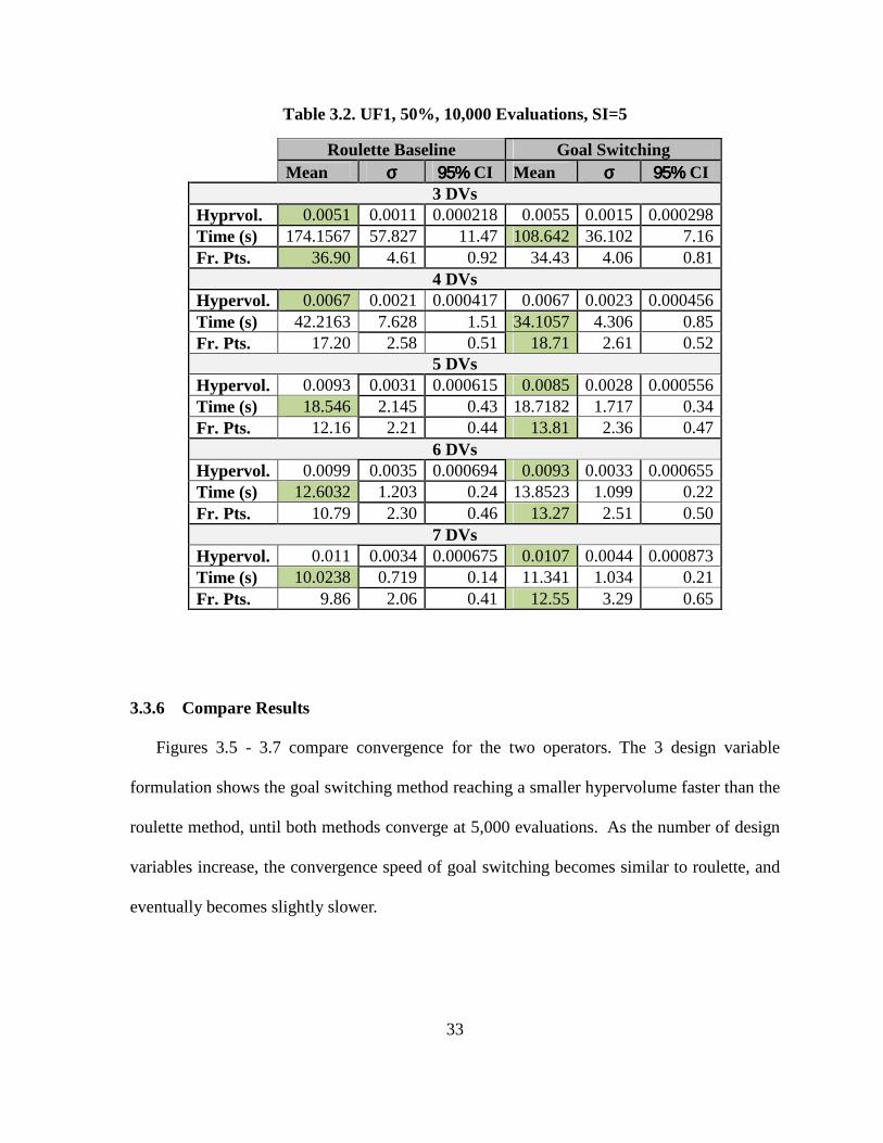
Table 3.2. UF1, 50%, 10,000 Evaluations, SI=5

Roulette Baseline Goal Switching Mean σσσσ 95% 95% 95% 95% CI Mean σσσσ 95% 95% 95% 95% CI

3 DVs Hyprvol. 0.0051 0.0011 0.000218 0.0055 0.0015 0.000298 Time (s) 174.1567 57.827 11.47 108.642 36.102 7.16 Fr. Pts. 36.90 4.61 0.92 34.43 4.06 0.81

4 DVs Hypervol. 0.0067 0.0021 0.000417 0.0067 0.0023 0.000456 Time (s) 42.2163 7.628 1.51 34.1057 4.306 0.85 Fr. Pts. 17.20 2.58 0.51 18.71 2.61 0.52




3.3.6 Compare Results

Figures 3.5 - 3.7 compare convergence for the two operators. The 3 design variable

formulation shows the goal switching method reaching a smaller hypervolume faster than the

roulette method, until both methods converge at 5,000 evaluations. As the number of design

variables increase, the convergence speed of goal switching becomes similar to roulette, and

eventually becomes slightly slower.

34

Figure 3.5. Convergence of Goal Switching and Roulette on UF1 for 3 DVs, 50%


35


Table 3.3 shows the effects of changing the selection percentage value. A smaller

selection percentage of 25% improves the hypervolume metric but has a negative effect on

run time. This percentage also increases the number of points on the frontier. As the

percentage increases, all metrics – hypervolume, time required, and the number of frontier

points – decrease. Results in this table are the average results after 100 runs with the stated

variables. CI is shorthand for 95% confidence interval. Because the CI overlap for the

hypervolume data, definite conclusions cannot be drawn as to which technique is better until

more data points are collected.

36

Table 3.3. UF1, 4 DVs, 10,000 Evaluations, SI=5

Roulette Baseline Goal Switching Mean σσσσ 95% CI Mean σσσσ 95% CI

25% Selection Hyprvol. 0.0069 0.0020 4.0e-4 0.0064 0.0022 4.4e-4 Time (s) 42.734 7.713 1.53 65.024 12.283 2.44 Fr. Pts. 16.88 2.57 0.51 21.174 3.31 0.66



Figures 3.8 and 3.9 show convergence rates for selection percentage values of 25% and

75% when the problem has 4 design variables. From these figures, it can be seen that both

converge faster than the standard 50% with 4 variables. A value of 25% also yields

significant initial improvement in the hypervolume metric.

37



38

3.4 Chapter Summary

This chapter outlined the steps needed to implement a selection method enhanced by goal

switching. First, the goals of the optimization should be defined in the context of which

characteristics of the Pareto frontier are most important to the designer. Next, the parameters

of cut percentage, switching index, and switching mode should be selected. Finally, a

standard selection operator should be chosen to allow the results to be passed to the crossover

and mutation operators. This selection operator is needed because goal switching acts as a

filter and does not select candidates to be passed to other operators. The chapter also showed

that the addition goal switching to a selection operator can improve the Pareto frontier when

defined by metrics like hypervolume, time to convergence, and number of frontier points.

The next chapter will look into how the goal switching parameters can be altered to find the

best combination for optimizing each metric.

39

4. GOAL SWITCHING PARAMETER ANALYSIS

4.1 Introduction

While the previous chapter defined the goal switching method and demonstrated the

possible advantages, a more detailed analysis is needed to understand the effects each

parameter has on algorithm performance. To reduce the computational overhead associated

with the parameter study, a testing plan using design of experiments was developed. If four

levels are selected for the three parameters of goal switching, 64 runs would have been

needed to analyze the different possibilities. However, given the design of experiments layout

shown in Table 4.1 based on a L’16 (45) orthogonal array setup, only 16 runs are needed. The

table should be read vertically for each case, with the first case having a switching mode

input of 1, a cut percentage input of 1, and a switching mode input of 1. Similarly, case 10

will have inputs of 3, 2, and 4 for switching mode, cut percentage, and switching mode

respectively. Tables in each subsection will describe exactly what input corresponds to each

number 1-4, as this portrayal is a generic representation of the four levels chosen.

Table 4.1. Goal Switching Design of Experiments Layout

Case 1 2 3 4 5 6 7 8 9 10 11 12 13 14 15 16 Switching 1 1 1 1 2 2 2 2 3 3 3 3 4 4 4 4

Cut % 1 2 3 4 1 2 3 4 1 2 3 4 1 2 3 4 Mode 1 2 3 4 2 1 4 3 3 4 1 2 4 3 2 1

40

The remainder of the experimental procedure, defined in Section 3.3, is run exactly the

same. For the two case study problems presented in this chapter, both roulette and

tournament selection modes are used. Further analysis and conclusions related to the success

of goal switching on roulette and tournament selection will be presented following the data

from the case studies. The six steps are listed again below as a reminder, as they will be the

template for each of the subsections in this chapter.

1) Define the problem

2) Define the assessment metrics

3) Define parameters for selection operator with goal switching

4) Run the MOGA with default selection operator

5) Run the MOGA with updated selection operator

6) Compare results

4.1.1 Design of Experiments Analysis

When the data is collected from the design of experiments runs in Table 4.1 it has to be

analyzed to extract the influence that each variable had on the solution quality metrics.

Further, it must be determined if the initial population used has a statistically significant

effect on the results. In this setup, each case has ten unique populations, with each population

being run ten times.

A case in this terminology is a combination of one of the four possible switching indexes,

one of the four cut percentages, and one of the four selection modes, as determined from

41

Table 4.1. Since there are two things that may have an effect on the outcome – initial

population and the particular parameter case – analyzing the data required a two-stage nested

design procedure [65]. Table 4.2 provides the formulation of the analysis of variance

calculation for this type of problem setup. The first column shows the sum of the squares, the

second shows the number of degrees of freedom, the third shows the mean square values, the

fourth shows the F0 values, and the last shows the P values.

Table 4.2. Analysis of Variance Data Layout

Hypervolume SS DOF MS F0 P Cases SSA DOFA MSA F0,A PA

Populations SSB(A) DOFB(A) MSB(A) F0,B(A) PB(A)

Error SSE DOFE MSE

Total SST DOFT

The equations used to fill Table 4.2 are listed below, as are the variables and their

associated meanings.

a = cases (1-16, baseline, 17 total)

b = populations (1-10, 10 total)

n = runs (1-10, 10 total)

y... = Total (sum of case totals)

yi.. = case total (sum of population totals)

yij. = population total (sum of run totals)

42

yijk = Run value

SSA= 1

bn∑ yi..

2 -y…

2

abnai=1 (4.1)

SSB(A)= 1n∑ ∑ y��.2+�� -

bn

ai=1 ∑ ,-..2.-=1 (4.2)

SSE= ∑ ∑ ∑ ,�� /�� +�� - n

ai=1 ∑ ∑ ,-�.20�=1.-=1 (4.3)

SST= ∑ ∑ ∑ ,�� /�� +�� -1…%2+/

ai=1 (4.4)

34�5 = . − 1 (4.5)

34�6(5) = .(0 − 1) (4.6)

34�7 = .0(� − 1) (4.7)

34�8 = .0� − 1 (4.8)

9:5 = ::5 34�5⁄ (4.9)

9:6(5) = ::6(5) 34�6(5)⁄ (4.10)

9:7 = ::7 34�7⁄ (4.11)

F0 is for fixed A and B [65]

�<,5 = 9:5/9:7 (4.12)

�<,6(5) = 9:6(5)/9:7 (4.13)

P-Values were determined using the fcdf command in Matlab [64], which is a cumulative

distribution function. The inputs are F0,A, DOFA, and DOFE for P-0A and F0,B(A), DOFB(A),

and DOFE for P-0B(A).

43

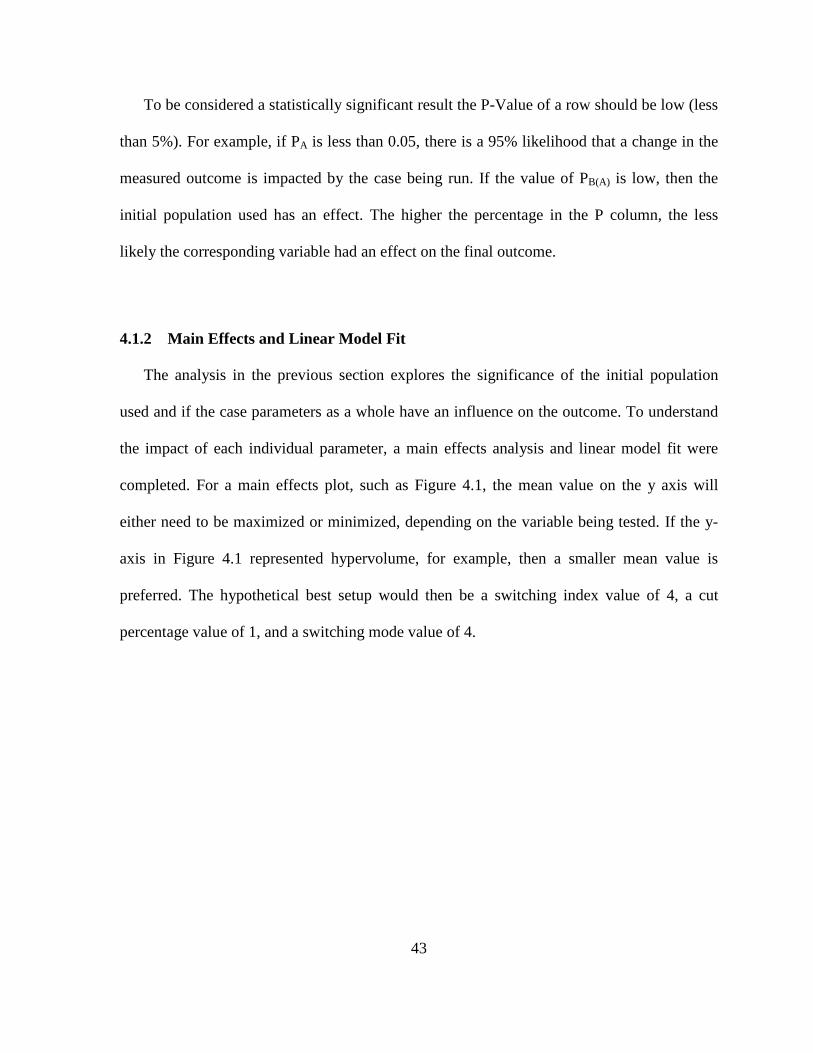
To be considered a statistically significant result the P-Value of a row should be low (less

than 5%). For example, if PA is less than 0.05, there is a 95% likelihood that a change in the

measured outcome is impacted by the case being run. If the value of PB(A) is low, then the

initial population used has an effect. The higher the percentage in the P column, the less

likely the corresponding variable had an effect on the final outcome.

4.1.2 Main Effects and Linear Model Fit

The analysis in the previous section explores the significance of the initial population

used and if the case parameters as a whole have an influence on the outcome. To understand

the impact of each individual parameter, a main effects analysis and linear model fit were

completed. For a main effects plot, such as Figure 4.1, the mean value on the y axis will

either need to be maximized or minimized, depending on the variable being tested. If the y-

axis in Figure 4.1 represented hypervolume, for example, then a smaller mean value is

preferred. The hypothetical best setup would then be a switching index value of 4, a cut

percentage value of 1, and a switching mode value of 4.

44

Figure 4.1. Example Main Effects Plot

As in the previous section, there is a relationship between the index used to represent the

x-axis in the main effects plot and the true value for each parameter. For reference, an

example of this mapping relationship is shown in Table 4.3.

Table 4.3. Example Mapping Relationship between Index Number and Parameter Setting

1 2 3 4

Switching (gen.) 3 5 10 20

Cut % 25 50 75 100

Mode f1,f2 f1,f2,both f1,both,f2 f1,both,f2,both

45

The results from the linear model fit, whose form is shown in Equation 4.14, will be

shown in table form. In equation 4.14, β represents the parameter being estimated, X

represents the value of that parameter, and ϵ represents the error.

>� = ?< + ? @� + ? @� +⋯+ ?/@�/ + B� (4.14)

In such tables, the first setting for each parameter is omitted. This omission is done

because the model is fit using a dummy-encoding scheme. Under this scheme, it is assumed

that the value of the first setting for each parameter is 0, establishing a baseline by which to

measure the impact of changing the value of the parameter. Further, the intercept value

reports the estimate of the performance metric when these baseline settings are used.

As shown in Table 4.4, every parameter besides the baseline is reported by including both

a P-Value and an estimate of the coefficient (β). Here, the P-Value is significant if the value

is less than 5%. The estimate of the coefficient reports if that particular parameter value has a

positive or negative effect on the performance metric being measured. The strength of this

effect is represented by the magnitude of that number.

For example, switching indices of 10 and 20 generations have statistically significant P-

Values, and both have a negative coefficient estimate. Further, the effect of the 20 generation

switch is larger than the 10 generation switch. However, a 5 generation switching index does

not have a statistically significant impact on the results since the P-Value is greater than 0.05

(or 5%).

46

Table 4.4. Example Linear Model Fit Data Layout

Hypervolume Estimate Se Tstat Pvalue Intercept 0.449139 0.003734 120.2785 0 5 Switch -0.00452 0.003207 -1.41E+00 0.158764 10 Switch -0.01701 0.003734 -4.55445 5.65E-06 20 Switch -0.02293 0.003312 -6.92121 6.47E-12 50% 0.005247 0.003448 1.521793 0.12826 75% 0.005972 0.003448 1.73231 0.083412 100% 0.005838 0.003448 1.693214 9.06E-02 C1 -0.00625 0.003312 -1.88536 0.059563 C2 -0.0132 0.003448 -3.8291 0.000134 C3 -0.01693 0.003312 -5.11097 3.59E-07

Having defined the mathematical foundation of the analysis needed for this chapter, the

following sections explore the effect of goal switching in two case study problems.

4.2 CASE STUDY 1 – MP3 Player Product Line Design Problem

This section explores the design of an MP3 player product line where the objectives of

the problem are two maximize a surrogate of price and market share of preference. Each sub-

section corresponds to the six step experimental procedure introduced in Chapter 3.


Consider a company that is interested in producing a product line of MP3 players. The

design problem they face is making decisions about the configuration of the product line

when considering the performance objectives of market share of preference and a surrogate

47

measure of profit. Analyzing these two objectives requires a mathematical representation of

customer preference for the different product components that the company can choose from

and the price of each product in the line. To get this information, customer reference data was

obtained using a choice-based conjoint survey using Sawtooth Software SSI Web [66]. Table

4.5 shows the breakdown of the seven product attributes and the price levels used in the

survey.

Table 4.5. MP3 Player Attributes and Price Levels

Levels Photo/ Video/ Camera

Web/ App/ Ped

Input Screen

Size Storage

Background Color

Background Overlay

Price

1 None None Dial 1.5 in diag

2 GB Black No pattern /

graphic overlay

$49

2 Photo only Web only

Touch-pad

2.5 in diag

16 GB White Custom pattern overlay

$99

3 Video only App only Touch-screen

3.5 in diag

32 GB Silver Custom graphic overlay

$199

4 Photo and

Video Only

Ped only Buttons 4.5 in diag

64 GB Red

Custom pattern and

graphic overlay

$299

5 Photo and

lo-res camera

Web and App only

5.5 in diag

160 GB Orange

$399

6 Photo and

hi-res camera

App and ped only

6.5 in diag

240 GB Green $499

7

Photo, video and

lo-res camera

Web and Ped only

500 GB Blue $599

8 Photo,video and hi-

res camera

Web, app, and

ped 750 GB Custom $699

48

To get mathematical representations of customer preference for each feature and price

level, a hierarchical Bayes (HB) mixed logit model was fit using Sawtooth Software

CBC/HB [67] to estimate the observed part-worths for each respondent. The data used to fit

the model came from 205 choice-based conjoint surveys containing twelve choice tasks each.

This model was fit using the default settings and the part-worths for the price levels were

constrained to be monotonically decreasing (i.e. the part-worth for $49 is greater than the

part-worth for $99). For each of the 205 respondents, fifty-five total part-worths are

calculated: forty-six for the features, eight for the price levels, and one for the outside good.

The outside good is the share of the combined shares of the inside goods subtracted from the

total potential market size.

Estimating market share of preference [68] is done by predicting the probability (C) that a

respondent will select a certain product over the rest of the field. In Equation 4.15, the

probability of selecting the -DE product is predicted by dividing the exponential of the

observed utility (F) of the -DE product by the sum of the exponentials of all � products under

consideration (including the outside good). A respondent’s share of preference for a product

line is merely the summation of all the individual product preference shares. This value can

then be aggregated across all respondents in the survey to get a market share of preference of

the product line.

C� = GHI∑ GHJ/��

(4.15)

The second objective (Equation 4.16) considered in this problem is per capita

contribution margin (PCCM). This objective acts as a profit surrogate since the cost model

49

used only includes the feature cost of the product being sold. Contribution margin is the

difference between a product’s selling price (K) and its cost (L); it does not account for

investments, other fixed costs, or the time value of money. Equation 4.16 shows the

formulation of the per capita contribution margin for the -DE product in the product line. To

get the PCCM for a product line, simply sum the PCCM for each product.

KLL9� = (K� − L�) ∗ C� (4.16)

The cost model for the MP3 market simulator, shown, in Table 4.6 was constructed by

first allocating the difference in the manufacturer’s suggested retail price (MSRP) of different

iPods to the various features in Table 4.5 and then dividing those values in half. This model

assumes that the MSRP of an iPod is a 100% markup of its cost. Note that iPods were used

only to build the cost model as they presented a large amount of feature diversity from a

single manufacturer. To ensure that the MSRP of all potential products fell within the price

levels used in the survey ($49-$699), a base price of $52 was selected and the maximum

amount of markup was limited to 100%.

50

Table 4.6. MP3 Player Cost Per Feature

Levels Photo/ Video/

Camera

Web/ App/ Ped

Input Screen

Size Storage

Background Color

Background Overlay

1 $0.00 $0.00 $0.00 $0.00 $0.00 $0.00 $0.00 2 $2.50 $10.00 $2.50 $12.50 $22.50 $5.00 $2.50 3 $5.00 $10.00 $20.00 $22.50 $60.00 $5.00 $5.00 4 $7.50 $5.00 $10.00 $30.00 $100.00 $5.00 $7.50 5 $8.50 $20.00

$35.00 $125.00 $5.00

6 $15.00 $15.00 $40.00 $150.00 $5.00

7 $16.00 $15.00

$175.00 $5.00

8 $21.00 $25.00 $200.00 $10.00

As the firm would ideally like to maximize both of these objectives, they are

reformulated into minimizations by multiplying by negative one. Further, it was decided that

the company would design five products for the line. This decision led to a problem

formulation with 81 design variables: 46 price markup variables (continuous variables

between 0 and 1) and 35 product configuration variables (7 per product represented as integer

variables).


Hypervolume, number of frontier points, and crowding distance were used to compare

the results and assess the effectiveness of the different goal-switching strategies. For this

problem, hypervolume and crowding distance were minimized while number of frontier

points was maximized.

51


To accommodate the design of experiments structure shown in Table 4.1, 4 different

values of each of the three parameters were chosen. Each value can be seen in Table 4.7, and

these values correspond to the numbers 1-4 on the main effects plots for this problem. The

first variable is switching index as a function of generations (Switching), the second is

selection percentage (Cut %), and the last is switching mode (Mode).

Table 4.7. Design of Experiments MP3 Reference

1 2 3 4 Switching (gen.) 3 5 10 20

Cut % 25 50 75 100


Switching index was bounded between 3 generations and 20 generations so the effect of

quickly switching or slowly switching could be observed. The generation limit was set to

100, so a switching index of 20 cycles through each of the objectives once for the (f1, both,

f2, both) case and leaves a few generations at the beginning for burn-in. Having a lower

bound of 3 allows for each mode to optimized at least 8 times while still pausing on each

objective. By optimizing for both objectives simultaneously in some of the switching modes,

it was hypothesized that the solutions on the Pareto frontier would be more evenly

distributed. This structure also allows the influence of the “both” mode to be observed.

Further, two different standard selection operators were chosen: roulette and tournament.

Each set of experiments shown in Table 4.1 was run for both selection operators.

52


For each experiment in Table 4.1, 10 replications were run for 10 unique starting

populations. Objective 1 is the normalized market share of preference (originally from 0% to

100%) and objective 2 represents the surrogate measure of profit (PCCM). The settings for

the MOGA used in this study were:


• Encoding: real-value and integer




• Convergence: 80,000 function evaluations

The results in Table 4.8 show the average hypervolume (Hyp.), average number of points

on the frontier (Frnt.Pts.), and average crowding distance (Crd.Dst.) along with the standard

deviation and 95% confidence interval for the baseline case run. The hypervolume is

calculated by adding 1 to the x-axis solutions and adding 120 to the y-axis solutions, then

dividing by 0.35 for the x-axis and 120 for the y-axis to normalize the axes to 1. These

numbers are problem specific and come from the maximum values possible for each

objective.

53

Table 4.8. Baseline Results, MP3 Problem

Hyp. σ CI Frnt.Pts. σ CI Crd.Dst. σ CI Roulette 0.4525 0.015 2.98E-03 113.86 10.9034 2.16 0.0783 0.0083 1.65E-03 Tourn. 0.4099 0.0147 2.92E-03 233.76 29.9479 5.94 0.05 0.0077 1.53E-03

The hypervolume and crowding distance should be minimized for optimum results and

the frontier points should be maximized for the same reason. Here it is easy to see that the

tournament selection method is more effective at finding frontier points as well as

minimizing hypervolume and crowding distance.


Tables 4.9-4.14 and Figures 4.2-4.7 show the results from the various runs when the

roulette and tournament selection operators are enhanced with goal switching. The tables

show the two-stage nested design statistical analysis explained earlier.

54

Table 4.9. MP3 Roulette Selection Analysis of Variance Results

Hypervolume SS DOF MS F0 P-Value

Cases 0.269135 16 0.016821 7.756971 0.00E+00 Populations 0.275672 153 1.80E-03 0.830889 0.929624 Error 3.317798 1530 2.17E-03 Total 3.862605 1699

Frontier Points SS DOF MS F0 P-Value

Cases 3.42E+06 16 2.14E+05 18.5785 0 Populations 1.07E+06 153 6.97E+03 0.60527 0.999947 Error 1.76E+07 1530 1.15E+04 Total 2.21E+07 1699

Crowding Distance SS DOF MS F0 P-Value

Cases 3.46E-01 16 0.021599 1.88E-06 1 Populations 3.40E-01 153 0.002223 1.93E-07 1 Error 4.12E+00 1530 0.00269 Total 4.80E+00 1699

In Table 4.9 it can be seen that the change in hypervolume and frontier points is

statistically significant when the case is changed, but not when the population is changed.

This is desired as the outcome of the results will not be influenced by the starting points but

rather the process of selection. However, for crowding distance, neither the case used or the

starting population have a statistically significant impact on the results.

The variables mode 2, mode 3, and mode 4 represent the other three selection modes not

represented by the baseline, selection modes 2, 3, and 4 respectively from the table in section

4.1.4.

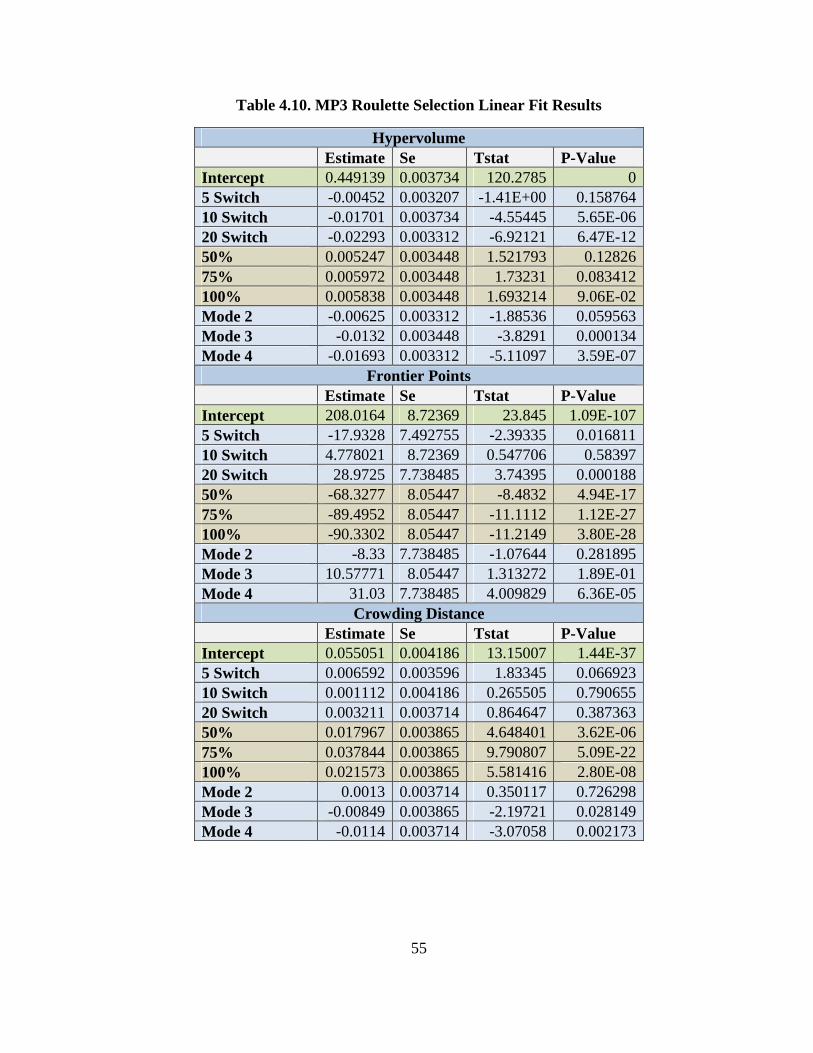
55

Table 4.10. MP3 Roulette Selection Linear Fit Results

Hypervolume Estimate Se Tstat P-Value

Intercept 0.449139 0.003734 120.2785 0 5 Switch -0.00452 0.003207 -1.41E+00 0.158764 10 Switch -0.01701 0.003734 -4.55445 5.65E-06 20 Switch -0.02293 0.003312 -6.92121 6.47E-12 50% 0.005247 0.003448 1.521793 0.12826 75% 0.005972 0.003448 1.73231 0.083412 100% 0.005838 0.003448 1.693214 9.06E-02 Mode 2 -0.00625 0.003312 -1.88536 0.059563 Mode 3 -0.0132 0.003448 -3.8291 0.000134 Mode 4 -0.01693 0.003312 -5.11097 3.59E-07

Frontier Points Estimate Se Tstat P-Value

Intercept 208.0164 8.72369 23.845 1.09E-107 5 Switch -17.9328 7.492755 -2.39335 0.016811 10 Switch 4.778021 8.72369 0.547706 0.58397 20 Switch 28.9725 7.738485 3.74395 0.000188 50% -68.3277 8.05447 -8.4832 4.94E-17 75% -89.4952 8.05447 -11.1112 1.12E-27 100% -90.3302 8.05447 -11.2149 3.80E-28 Mode 2 -8.33 7.738485 -1.07644 0.281895 Mode 3 10.57771 8.05447 1.313272 1.89E-01 Mode 4 31.03 7.738485 4.009829 6.36E-05

Crowding Distance Estimate Se Tstat P-Value

Intercept 0.055051 0.004186 13.15007 1.44E-37 5 Switch 0.006592 0.003596 1.83345 0.066923 10 Switch 0.001112 0.004186 0.265505 0.790655 20 Switch 0.003211 0.003714 0.864647 0.387363 50% 0.017967 0.003865 4.648401 3.62E-06 75% 0.037844 0.003865 9.790807 5.09E-22 100% 0.021573 0.003865 5.581416 2.80E-08 Mode 2 0.0013 0.003714 0.350117 0.726298 Mode 3 -0.00849 0.003865 -2.19721 0.028149 Mode 4 -0.0114 0.003714 -3.07058 0.002173

56

Figure 4.2. MP3 Hypervolume Main Effects Plot, Roulette Selection

Figure 4.3. MP3 Crowding Distance Main Effects Plot, Roulette Selection

57

Figure 4.4. MP3 Frontier Points Main Effects Plot, Roulette Selection

From Figure 4.2 and Table 4.10 it can be seen that a switching index of 20, a cut

percentage of 25%, and a switching mode of (f1, both, f2, both) has the greatest chance of

producing an optimally low hypervolume for this case study. The smallest crowding distance

is desired, so Figure 4.3 and Table 4.10 show a switching index of 5, a cut percentage of

25%, and a switching mode of (f1, both, f2, both) has the greatest chance of minimizing this

value. Two out of the three variable values match for these metrics which means they might

be able to be optimized together. For frontier points a maximum is desired so a switching

index of 20, a cut percentage of 25%, and a mode of (f1, both, f2, both) is desired, as can be

seen from Table 4.10 and Figure 4.4. All of these variable values match with the

hypervolume optimization, so hypervolume and frontier points can be optimized together

58

with the same settings. Table 4.11 shows a summary of results for the goal switching with

roulette selection operator. Comparing the winners in Table 4.11 to Table 4.10, the

switching index and switching mode both are significant for the hypervolume since they have

a Pvalue below 5% compared to the baseline. For crowding distance, switching mode 4 is

under 5% for the Pvalue so is significant with respect to the baseline goal switching case.

Again, 25% cut percentage is on the baseline. Finally, switching index and switching mode

are significant with respect to the baseline for the number of frontier points, but cut

percentage is on the baseline goal switching case.

Table 4.11. MP3 Main Effects Plot Summarized Results, Roulette Selection

Hypervolume 1 2 3 4 Switching 3 5 10 20

Cut % 25 50 75 100


Crowding Distance 1 2 3 4 Switching 3 5 10 20

Cut % 25 50 75 100


Frontier Points 1 2 3 4 Switching 3 5 10 20

Cut % 25 50 75 100


Tables 4.12-4.14 and Figures 4.5-4.7 show the data for the tournament selection operator.

Again the analysis shows that the hypervolume and the number of frontier points are

59

significantly changed by the cases and not the populations. Also, crowding distance is not

changed in a statistically significant way by altering the cases or the populations.

Table 4.12. MP3 Tournament Selection Analysis of Variance Results


Cases 0.823738 16 0.051484 23.2589 0.00E+00 Populations 0.288979 153 1.89E-03 0.853287 0.896426 Error 3.386657 1530 2.21E-03 Total 4.499374 1699


Cases 3.45E+06 16 2.15E+05 13.48083 0 Populations 2.00E+06 153 1.31E+04 0.818175 0.944635 Error 2.45E+07 1530 1.60E+04 Total 2.99E+07 1699


Cases 2.63E-01 16 0.016434 1.03E-06 1 Populations 2.30E-01 153 0.001506 9.42E-08 1 Error 3.14E+00 1530 0.00205 Total 3.63E+00 1699

60

Table 4.13. MP3 Tournament Selection Linear Fit Results


Intercept 0.469055 0.003829 122.5141 0 5 Switch -0.00271 0.003288 -8.24E-01 0.410198 10 Switch -0.01792 0.003829 -4.6806 3.10E-06 20 Switch -0.02875 0.003396 -8.46472 5.75E-17 50% -0.01306 0.003535 -3.69538 0.000227 75% -0.02179 0.003535 -6.16451 8.95E-10 100% -0.0316 0.003535 -8.93865 1.07E-18 Mode 2 -0.01675 0.003396 -4.93081 9.05E-07 Mode 3 -0.02562 0.003535 -7.24664 6.64E-13 Mode 4 -0.03068 0.003396 -9.03362 4.69E-19


Intercept 139.4995 10.02682 13.91263 1.31E-41 5 Switch -32.0322 8.612015 -3.71948 0.000207 10 Switch 15.57365 10.02682 1.553198 0.120575 20 Switch 37.8125 8.89445 4.251246 2.25E-05 50% 6.866042 9.257637 0.741662 0.458401 75% 16.14104 9.257637 1.743538 0.081433 100% 44.83104 9.257637 4.842601 1.41E-06 Mode 2 24.02 8.89445 2.70056 0.006996 Mode 3 68.70146 9.257637 7.421057 1.88E-13 Mode 4 63.7625 8.89445 7.168796 1.15E-12


Intercept 0.074833 0.00361 20.72878 1.11E-84 5 Switch 0.008406 0.003101 2.71111 0.006778 10 Switch -0.00306 0.00361 -0.8468 0.397235 20 Switch -0.00901 0.003202 -2.81247 0.004977 50% 0.002313 0.003333 0.69389 0.487852 75% 0.006299 0.003333 1.889722 0.058977 100% -0.00955 0.003333 -2.86651 4.20E-03 Mode 2 -0.01109 0.003202 -3.46421 0.000546 Mode 3 -0.0225 0.003333 -6.74981 2.07E-11 Mode 4 -0.01951 0.003202 -6.09283 1.39E-09

61

Figure 4.5. MP3 Hypervolume Main Effects Plot, Tournament Selection

Figure 4.6. MP3 Crowding Distance Main Effects Plot, Tournament Selection

62

Figure 4.7. MP3 Frontier Points Main Effects Plot, Tournament Selection

From Figures 4.5 and 4.7 the optimum variable inputs for hypervolume and number of

frontier points can be seen to be the same as the roulette operator: a switching index of 20, a

cut percentage of 100%, and a switching mode of (f1, both, f2, both). Crowding distance is

almost the same, with switching mode being almost even between (f1, both, f2, both) and (f1,

both, f2). More than likely they could all be optimized together, especially since changing the

cases does not have any statistically significant effect on the crowding distance. Table 4.14

summarizes these results. According to Table 4.13, all of the hypervolume parameters that

are highlighted are significantly better than the baseline goal switching parameters used for

comparison. The same can be said for the frontier points parameters, but not for the

crowding distance parameters since switching index has a Pvalue above 5% and cut

63

percentage is on the baseline. The crowding distance is the only parameter to be significant

with respect to the baseline for the crowding distance metric.

Table 4.14. Main Effects Plot Summary Tournament MP3


Cut % 25 50 75 100



Cut % 25 50 75 100



Cut % 25 50 75 100



Tables 4.15-4.18 show the results for the second part of the MP3 case study problem,

analyzed using the two-stage nested design addition method and a mean analysis method.

Both analysis methods agree with each other, so the confidence intervals and standard

deviation are reliable. The roulette data is very strong, with case 1 being the only parameter

combination resulting in a hypervolume score worse than the baseline. Crowding distance

64

has a worse score than the baseline in cases 3, 7, 11, 15, and 16, but still achieves a higher

score more than 66% of the time.

Data for the tournament method is not nearly as strong, with the hypervolume and

frontier points only having higher than baseline results 4 of 16 times, and crowding distance

only scoring higher than the baseline 3 of 16 times. It is unclear why goal switching does not

work as well on tournament for this specific problem.

Table 4.15. MP3 Roulette Mean Analysis

Hyp σ CI Frnt.Pts σ CI Crd.Dst σ CI 1 0.4567 0.0257 5.10E-03 209.40 45.0575 8.94 0.0557 0.0103 2.04E-03 2 0.4417 0.0136 2.70E-03 144.96 21.3253 4.23 0.0735 0.018 3.57E-03 3 0.4385 0.0105 2.08E-03 133.05 15.9428 3.16 0.08 0.0205 4.07E-03 4 0.4403 0.0091 1.81E-03 129.78 10.7705 2.14 0.0698 0.0075 1.49E-03 5 0.4390 0.0157 3.11E-03 163.54 37.5169 7.44 0.0638 0.0095 1.88E-03 6 0.4463 0.0083 1.65E-03 136.37 11.0012 2.18 0.0764 0.0168 3.33E-03 7 0.4370 0.0159 3.15E-03 132.44 17.273 3.43 0.0857 0.0188 3.73E-03 8 0.4333 0.0078 1.55E-03 135.88 18.2172 3.61 0.0744 0.0135 2.68E-03 9 0.4351 0.0152 3.02E-03 177.89 26.1544 5.19 0.0581 0.0077 1.53E-03

10 0.4267 0.0199 3.95E-03 154.01 22.0058 4.37 0.067 0.0134 2.66E-03 11 0.4321 0.0079 1.57E-03 129.35 23.2894 4.62 0.0953 0.016 3.17E-03 12 0.4314 0.0108 2.14E-03 129.57 15.1432 3.00 0.0735 0.0145 2.88E-03 13 0.3974 0.0109 2.16E-03 307.62 58.5387 11.61 0.0404 0.0066 1.31E-03 14 0.4220 0.0066 1.31E-03 172.51 25.565 5.07 0.0675 0.0124 2.46E-03 15 0.4320 0.0094 1.86E-03 128.34 21.843 4.33 0.1029 0.0266 5.28E-03 16 0.4341 0.0104 2.06E-03 124.61 14.667 2.91 0.0811 0.0169 3.35E-03

Base 0.4525 0.015 2.98E-03 113.86 10.9034 2.16 0.0783 0.0083 1.65E-03

65

Table 4.16. MP3 Roulette Nested Analysis

Supplier Tot Hyp Crddst Frpts Case 1 45.6708 5.569031 20940 Case 2 44.17381 7.351719 14496 Case 3 43.84903 7.996415 13305 Case 4 44.02992 6.982055 12978 Case 5 43.89514 6.382399 16354 Case 6 44.62708 7.640711 13637 Case 7 43.69768 8.573944 13244 Case 8 43.32567 7.442272 13588 Case 9 43.51074 5.811939 17789 Case 10 42.672 6.696067 15401 Case 11 43.21085 9.531976 12935 Case 12 43.14488 7.348804 12957 Case 13 39.74419 4.03704 30762 Case 14 42.19814 6.750637 17251 Case 15 43.20381 10.28739 12834 Case 16 43.40698 8.108523 12461 Baseline 45.24829 7.83487 11386

Table 4.17. MP3 Tournament Mean Analysis


10 0.4146 0.0112 2.22E-03 199.43 28.5952 5.67 0.0595 0.0077 1.53E-03 11 0.4220 0.0110 2.18E-03 189.68 57.1472 11.34 0.0742 0.0157 3.11E-03 12 0.4030 0.0087 1.73E-03 231.73 51.6737 10.25 0.0501 0.0103 2.04E-03 13 0.3917 0.0091 1.81E-03 281.18 40.8652 8.11 0.0397 0.0093 1.85E-03 14 0.4122 0.0062 1.23E-03 248.06 54.6549 10.84 0.0474 0.0096 1.90E-03 15 0.4121 0.0081 1.61E-03 190.80 35.6605 7.08 0.0671 0.0159 3.15E-03 16 0.4057 0.0058 1.15E-03 213.53 29.7968 5.91 0.055 0.0085 1.69E-03

Base 0.4099 0.0147 2.92E-03 233.76 29.9479 5.94 0.05 0.0077 1.53E-03

66

Table 4.18. MP3 Tournament Nested Analysis


After studying the MP3 problem with a design of experiments, it is clear that the

parameter values chosen for the goal switching selection operator can play a large part in

altering the Pareto frontier metrics. The P-Values in Tables 4.9 and 4.12 show that both

hypervolume and the number of frontier points can be altered by changing the goal switching

parameters, and that this effect is statistically significant. Having 10 different starting

populations had no statistical effect on the results, also evident from looking at the P-values

in Tables 4.9 and 4.12 and seeing values very close to 1. Crowding distance, the third

performance metric, was not affected by the goal switching parameters or by the starting

population, which is slightly surprising given that the frontier points are impacted by

changing the parameters of the selection operator. Picking crowding distance as the third

67

metric was done partially because changing the number of points on the Pareto frontier

should change the crowding distance. The number of points added to the frontier must have

not resulted in a large enough spread of points along the frontier to reduce the crowding

distance.

Looking at Table 4.10, the P-Values show that not all parameters significantly changed

the results of the performance metrics for the goal switching with roulette selection operator.

Compared to the baseline parameter setup (switching index of 3, cut percentage of 25%,

switching mode of f1, f2), only values of 10 and 20 for the switching index resulted in

significant changes to the hypervolume. All of the cut percentage parameters tested above

25% resulted in a higher hypervolume. Each switching mode that included an optimization

cycle on all the objectives at once lowered the hypervolume significantly except (f1, f2,

both). Switching the order of the objectives being optimized in the cycle changed the effects

on the hypervolume and the frontier points. Altering the number of frontier points compared

to the baseline parameters could be done with statistical significance by using a switching

index of 5 or 20, any cut percentage tested, or by using a switching mode of (f1, both, f2,

both). Unfortunately, the frontier point metric could only be improved by using a switching

index of 20 or the switching mode (f1, both, f2, both); the rest of the parameters mentioned

decreased the score performance metric score. Changing the switching index to 20 resulted

in the highest change to the hypervolume metric, improving it by 5%. A switching mode of

(f1, both, f2, both) improved the hypervolume by roughly 4%. Using a switching index of 20

improved the number of frontier points by 14% while a switching mode of (f1, both, f2, both)

results in a 15% improvement.

68

Table 4.13 shows the P-value results for goal switching with tournament selection. The

same baseline parameters from the goal switching with roulette selection were used, and the

results were similar. Hypervolume was decreased significantly by using a switching index of

10 or 20 or any switching mode, with a switching value of 20 resulting in a 6% and a

switching mode of (f1, both, f2, both) giving a 7%. Unlike the roulette case, all cut

percentages decreased the hypervolume significantly, with a value of 100% resulting in a 7%

improvement. To improve the number of frontier points, a value of 10 or 20 for the

switching index can be used, along with any cut percentage and any switching mode. Only

the switching mode of 10 and the cut percentage of 50% were not significant. Choosing a

switching index of 20 results in a 27% improvement for the performance metric, while a cut

percentage value of 100% gives 32% improvement to the number of frontier points. The

biggest gain is seen by using a switching mode of (f1, both, f2), with a 49% improvement to

the frontier points performance metric. Changing the parameter values for any goal

switching selection operator seems to have a much larger effect on the number of frontier

points than the hypervolume, especially for the augmented tournament selection operator

case. More case studies are needed before this conclusion can be confirmed.

Figures 4.8-4.10 show a Pareto frontier comparison between two different switching

modes, (f1, f2) on the left side and (f1, f2, both) on the right side, both using goal switching.

By changing to the (f1, f2, both) switching mode, the Pareto frontier has a more even spread

of points. This holds true even when varying the selection percentage. It is clear that the

goal switching parameters can alter the way a Pareto frontier looks and where points

accumulate along the frontier.

69

Figure 4.8. Pareto Frontier for (f1, f2) Switching Mode (L) and (f1, f2, both) Switching

Mode (R), 25% Selection

Figure 4.9. Pareto Frontier for (f1, f2) Switching Mode (L) and (f1, f2, both) Switching

Mode (R), 50% Selection

70

Figure 4.10. Pareto Frontier for (f1, f2) Switching Mode (L) and (f1, f2, both) Switching Mode (R), 75% Selection

To find out if goal switching is only successful being applied to a roulette selection rather

than a tournament selection, more case studies must be evaluated. The next section

introduces a new case study that will again compare the goal switching selection procedure to

baseline selection operators to see if goal switching can improve the Pareto frontier metrics.

4.3 CASE STUDY 2 – Two Bar Truss Design

This section explores the design of a two bar truss with three design variables, two

constraints, and two objective functions. As before, each sub-section corresponds to the six

step experimental procedure introduced in Chapter 3.


For this problem, the design variables are the cross sectional areas of links AC and BC

and the vertical position of the load. Minimizing stress in link AC and minimizing the

amount of material used are the two performance objectives. A third objective was formed by

71

aggregating the number of constraint violations. The constraints represent the feasibility of

the design to be built by limiting the overall stress in the links (g1) and the overall lengths of

the beams (x1, x2, y). By aggregating constraint violations into a third objective, the goal

switching technique can be analyzed on problems greater than two dimensional. Before any

final solution quality metrics were calculated, the final population was filtered to include

only designs that did not violate a constraint. Figure 4.11 and Equations (4.17-4.19) below

help to fully define the problem [69].

Figure 4.11. Two Bar Truss Diagram

72

(4.17)

(4.18)

(4.19)


The metrics being applied are hypervolume, crowding distance, and frontier points. Time

is not being represented as runs took place on different computers and cannot be directly

compared. Additionally, since the number of function calls remains the same, the time

should be about the same as well. Hypervolume is measured as area under the curve with the

four points added for reference and the chart scaled as to not artificially extend the penalty

area boxes. Crowding distance is only measured based on points on the frontier, and frontier

points is the number of points on the smallest ranked Pareto frontier.

73


Design of experiments analysis was also performed for this case study, so there were

again 4 different variations of each of the three variables. Table 4.19 shows the variable

references for the design of experiments.

Table 4.19. Design of Experiments Two Bar Reference

1 2 3 4 Switching (gen.) 3 5 10 20

Cut % 25 50 75 100

Mode f1,f2,f3 f1,f2,f3,all f1,all,f2,all,f3 f1,all,f2,all,f3,all


Below is the parameter setup for the two bar truss default selection case:


• Encoding: real-value and integer




• Convergence: 600 function evaluations

74

Just as in the previous case study, the problem was first run with a standard roulette and

tournament selection operator. The results were recorded and are displayed in Table 4.20,

where the difference between the roulette and tournament hypervolumes is small but

tournament selection still holds the advantage. Tournament also provides more frontier points

and a smaller crowding distance.


The results from the goal switching cases can be seen in Tables 4.21-4.28 and Figures

4.12-4.17. Specifically the two-stage nested statistical analysis is shown, which is needed to

see if switching cases or population has an effect on the performance metrics. A P-value

below 5% means that the metric is affected by a statistically significant amount from

changing either the case or population. The expected result is that the cases will have a

significant effect on the metrics but that the 10 different fixed, random populations will not.

75

Table 4.20. Two Bar Roulette Selection Analysis of Variance Results


Cases 0.0176 16 0.0011 2.7096 2.85E-04 Populations 0.0277 153 1.81E-04 0.4472 1 Error 0.6198 1530 4.05E-04 Total 0.6651 1699


Cases 4.52E+05 16 2.83E+04 26.4638 0 Populations 7.41E+04 153 484.0025 0.4531 1 Error 1.63E+06 1530 1.07E+03 Total 2.16E+06 1699

Crowding Distance SS DOF MS F0 P-Value Cases 4.75E+00 16 0.2967 2.78E-04 1 Populations 9.11E-01 153 0.006 5.58E-06 1 Error 1.70E+01 1530 0.0111 Total 2.27E+01 1699

According to Table 4.21 it can be seen that the hypervolume and the number of frontier

points are significantly affected by changing the case, but not the population. Crowding

distance seems to show no significance when changing either case or population.

Tables 4.22, 4.24, 4.25 and Figures 4.12-4.17 show which variable combinations will be

the most effective for minimizing or maximizing each performance metric, as the case may

be. Hypervolume and crowding distance metric scores were minimized, while the frontier

point metric was maximized. The results are compared against the baseline of a switching

index of 3, a cut percentage of 25%, and a selection mode of (f1, f2, f3). Here the variables

mode 2, mode 3, and mode 4 represent the other selection modes, modes 2, 3, and 4

76

respectively from Table 4.2.1 in Section 4.2.4. Table 4.22 shows the significance of

changing parameters with respect to the baseline for roulette selection with goal switching,

while Table 4.23 shows the parameter combinations that result in the best possible metric

score according to the main effects plots in Figures 4.12-4.14. The tournament selection with

goal switching results are shown in Tables 4.23-4.25, while Table 4.26 shows a summary of

which parameters optimize each metric with information gathered from Figures 4.15-4.17.

77

Table 4.21. Two Bar Roulette Selection Linear Fit Results


Intercept 0.127881 0.001551 82.45135 0 5 Switch 0.001162 0.001332 8.72E-01 0.383074 10 Switch -0.00111 0.001551 -0.71369 0.475526 20 Switch 0.00099 0.001376 0.719278 0.472076 50% 0.002565 0.001432 1.791033 0.073478 75% 0.002922 0.001432 2.040466 0.041469 100% 0.008002 0.001432 5.587995 2.70E-08 Mode 2 -0.00044 0.001376 -0.31907 0.749715 Mode 3 -0.00032 0.001432 -0.22533 0.821754 Mode 4 0.00077 0.001376 0.559896 0.57563


Intercept 97.16333 2.588728 37.53323 2.56E-221 5 Switch 0.56 2.223452 0.251861 0.801181 10 Switch -1.76333 2.588728 -0.68116 0.495871 20 Switch -1.885 2.296372 -0.82086 0.411849 50% 8.535833 2.390139 3.57127 0.000366 75% 1.208333 2.390139 0.505549 0.613243 100% -29.4192 2.390139 -12.3086 2.54E-33 Mode 2 -4.6725 2.296372 -2.03473 0.042044 Mode 3 -9.89333 2.390139 -4.13923 3.67E-05 Mode 4 -9.6825 2.296372 -4.21643 2.62E-05


Intercept 0.181255 0.008137 22.27626 6.75E-96 5 Switch -0.00143 0.006989 -0.20491 0.837671 10 Switch 0.00108 0.008137 0.132715 0.894435 20 Switch 0.003813 0.007218 0.528214 0.597424 50% -0.01007 0.007512 -1.34035 0.180323 75% 0.004425 0.007512 0.589033 0.555923 100% 0.111599 0.007512 14.85509 7.66E-47 Mode 2 0.010725 0.007218 1.485849 0.137517 Mode 3 0.022144 0.007512 2.947667 0.003248 Mode 4 0.022353 0.007218 3.096946 0.001989

78

Figure 4.12. Two Bar Hypervolume Roulette Main Effects Plot

Figure 4.13. Two Bar Crowding Distance Roulette Main Effects Plot

79

Figure 4.14. Two Bar Frontier Points Roulette Main Effects Plot

Results from these main effects plots show that hypervolume is minimized with a

switching index of 3 or 10, a cut percentage of 25%, and a switching mode of (f1, f2, f3, all).

Number of frontier points are maximized if the switching index is 5, the cut percentage is

50%, and the switching mode is (f1, all, f2, all, f3, all). To minimize crowding distance, the

parameters would include a switching index of 5, a cut percentage of 50%, and a switching

mode of (f1, all, f2, all, f3, all). Some of these variable values are very close to other values

for being effective in optimizing their respective metrics so it might be possible to

compromise when choosing variable values to achieve an optimization of one metric and a

slightly less optimal optimization of the other metrics using one variable configuration. Table

4.23 summarizes the results. Looking back at Table 4.22, neither the switching index nor

80

switching mode parameter changes result in statistically significant advances over the

baseline goal switching parameters, while the cut percentage parameter that resulted in the

best hypervolume was on the baseline. Crowding distance had switching index and cut

percentage show improvement over the baseline, while the switching mode is not

significantly affected by switching parameters to another parameter setup. Finally, frontier

points showed no significant effect by changing to any parameter from the baseline values.

Table 4.22. Main Effects Plot Summary Roulette Two Bar


Cut % 25 50 75 100



Cut % 25 50 75 100



Cut % 25 50 75 100


Table 4.24 below shows again that changing the case had a statistically significant effect

on the results for the hypervolume and frontier points metrics, but not on the crowding

81

distance metric. It also shows that changing the population has no effect on the metrics, as

predicted.

Table 4.23. Two Bar Tournament Selection Analysis of Variance Results


Cases 0.00361 16 2.26E-04 0.675011 8.21E-01 Populations 0.030418 153 1.99E-04 0.594717 0.999969 Error 0.511471 1530 3.34E-04 Total 0.545499 1699


Cases 1.79E+05 16 1.12E+04 7.967365 0.00E+00 Populations 1.02E+05 153 6.70E+02 0.477376 1.00E+00 Error 2.15E+06 1530 1.40E+03 Total 2.43E+06 1699


Cases 4.95E-01 16 0.030943 2.21E-05 1 Populations 4.47E-01 153 2.92E-03 2.08E-06 1 Error 7.62E+00 1530 0.004979 Total 8.56E+00 1699

Tables 4.25 and 4.26 show which parameters result in a significant change to the baseline

metrics resulting from a goal switching with tournament selection operator. Figures 4.15-

4.17 show the main effects plots for determining which parameters should be selected to

optimize each metric.

82

Table 4.24. Two Bar Tournament Selection Linear Fit Results

Hypervolume Estimate Se Tstat P-Value Intercept 0.126876 0.001433 88.53896 0 5 Switch 0.001411 0.001231 1.15E+00 0.251951 10 Switch 0.000102 0.001433 0.070923 0.943468 20 Switch 0.001938 0.001271 1.524835 0.127499 50% 0.001907 0.001323 1.441626 0.149605 75% 0.001951 0.001323 1.474543 0.140534 100% 0.002421 0.001323 1.829817 6.75E-02 Mode 2 0.000121 0.001271 0.095305 0.924084 Mode 3 8.71E-05 0.001323 0.065845 0.947509 Mode 4 0.000126 0.001271 0.099167 0.921018

Frontier Points Estimate Se Tstat P-Value Intercept 104.4554 2.928712 35.66599 3.37E-205 5 Switch 3.00625 2.515464 1.195108 0.232223 10 Switch 0.799583 2.928712 0.273015 0.784877 20 Switch -0.635 2.59796 -0.24442 0.806935 50% 18.69667 2.704042 6.91434 6.78E-12 75% 11.88667 2.704042 4.395888 1.18E-05 100% -5.09583 2.704042 -1.88452 5.97E-02 Mode 2 -3.3375 2.59796 -1.28466 0.199098 Mode 3 -5.69667 2.704042 -2.10672 3.53E-02 Mode 4 -8.275 2.59796 -3.18519 1.47E-03

Crowding Distance Estimate Se Tstat P-Value Intercept 0.1690 0.0055 30.6425 0.0000 5 Switch -0.0045 0.0047 -0.9598 0.3373 10 Switch -0.0047 0.0055 -0.8483 0.3964 20 Switch 0.0018 0.0049 0.3757 0.7072 50% -0.0238 0.0051 -4.6676 0.0000 75% -0.0130 0.0051 -2.5482 0.0109 100% 0.0146 0.0051 2.8717 0.0041 Mode 2 0.0042 0.0049 0.8667 0.3863 Mode 3 0.0048 0.0051 0.9389 0.3479 Mode 4 0.0171 0.0049 3.5034 0.0005

83

Figure 4.15. Two Bar Hypervolume Tournament Main Effects Plot

Figure 4.16. Two Bar Crowding Distance Tournament Main Effects Plot

84

Figure 4.17. Two Bar Frontier Points Tournament Main Effects Plot

The results for the tournament selection with goal switching show optimizing

hypervolume involves selecting a switching index of 3, a cut percentage of 25%, and a

selection mode of (f1, f2, f3). Minimizing crowding distance involves variable values of 10

for switching index, 50% for cut percentage, and (f1, f2, f3) for selection mode. Finally,

maximizing the number of frontier points would occur by selecting a switching index of 5, a

cut percentage of 50%, and a switching mode of (f1, f2, f3). It is interesting to see that for the

same problem but differing selection operators the variable values needed to produce the best

results are different as well. Table 4.29 summarizes the results. Interestingly, each of these

metrics had at least one parameter on the baseline that resulted in a better metric score. In

the case of hypervolume, leaving the parameters set to the baseline values resulted in the best

85

metric score. For crowding distance, changing the cut percentage metric results in a

significantly significant change to the baseline, but changing the switching index does not.

The same thing occurs for frontier points for switching index and cut percentage, with only

cut percentage showing statistically significant changes compared to the goal switching with

tournament selection baseline.

Table 4.25. Main Effects Plot Summary Tournament Two Bar


Cut % 25 50 75 100



Cut % 25 50 75 100



Cut % 25 50 75 100



Both the summation method for a two-variable nested design and the mean method used

in the first two case studies are used to show if each case won or lost compared to the

86

baseline. In the case of the roulette data, the hypervolume only lost once in case 16, as did

the frontier points. The crowding distance metric lost 4 times in cases 4, 8, 12, and case 16

like the other two metrics. These results in tables 4.27-4.28 are similar to those seen with the

MP3 problem using roulette selection.

Table 4.26. Two Bar Truss Roulette Mean Analysis


10 0.1305 0.0038 7.54E-04 93.51 6.3049 1.25 0.1947 0.0204 4.05E-03 11 0.1287 0.0022 4.36E-04 98.15 7.8589 1.56 0.1853 0.0203 4.03E-03 12 0.1350 0.0057 1.13E-03 60.51 5.9912 1.19 0.306 0.0313 6.21E-03 13 0.1304 0.0053 1.05E-03 89.27 8.1025 1.61 0.2028 0.0262 5.20E-03 14 0.1294 0.0054 1.07E-03 92.54 8.4372 1.67 0.1963 0.0168 3.33E-03 15 0.1315 0.0036 7.14E-04 96.40 8.4702 1.68 0.1904 0.0178 3.53E-03 16 0.1377 0.0047 9.32E-04 58.98 5.8891 1.17 0.312 0.0406 8.06E-03

Base 0.1372 0.003 5.95E-04 59.39 6.2799 1.25 0.3008 0.0331 6.57E-03

87

Table 4.27. Two Bar Truss Roulette Nested Analysis


Tables 4.29-4.30 show the results for the tournament data. In this case the hypervolume is

never greater than the baseline, and again we see a link between crowding distance and

frontier points just as in the last case study. The frontier points and crowding distance

metrics lose 5 times each, similar to the amount of times that the crowding distance metric

loses in the roulette cases.

88

Table 4.28. Two Bar Truss Tournament Mean Analysis

hyp σ CI Frnt.Pts σ CI Crd.Dst σ CI 1 0.1256 0.0047 9.32E-04 103.34 4.7223 0.94 0.1673 0.0111 2.20E-03 2 0.1293 0.0032 6.35E-04 116.51 6.3049 1.25 0.1587 0.0149 2.96E-03 3 0.1283 0.0050 9.92E-04 109.70 6.2558 1.24 0.1638 0.0212 4.21E-03 4 0.1309 0.0055 1.09E-03 96.45 10.6767 2.12 0.1901 0.0185 3.67E-03 5 0.1282 0.0044 8.73E-04 107.40 8.9094 1.77 0.1631 0.0183 3.63E-03 6 0.1307 0.0042 8.33E-04 127.10 7.7953 1.55 0.1392 0.012 2.38E-03 7 0.1291 0.0042 8.33E-04 105.36 10.208 2.03 0.1783 0.0174 3.45E-03 8 0.1306 0.0042 8.33E-04 97.76 10.5057 2.08 0.1822 0.0185 3.67E-03 9 0.1295 0.0050 9.92E-04 102.17 9.022 1.79 0.1682 0.0148 2.94E-03

10 0.1284 0.0051 1.01E-03 118.59 11.3608 2.25 0.1503 0.0172 3.41E-03 11 0.1303 0.0032 6.35E-04 119.00 6.7539 1.34 0.1504 0.0109 2.16E-03 12 0.1288 0.0042 8.33E-04 92.05 3.1704 0.63 0.1914 0.0142 2.82E-03 13 0.1293 0.0040 7.94E-04 92.98 10.5895 2.10 0.1962 0.0338 6.71E-03 14 0.1306 0.0040 7.94E-04 116.27 6.6234 1.31 0.1515 0.0119 2.36E-03 15 0.1314 0.0042 8.33E-04 117.17 6.6993 1.33 0.1502 0.0127 2.52E-03 16 0.1306 0.0053 1.05E-03 97.04 7.0345 1.40 0.1894 0.0148 2.94E-03

Base 0.1317 0.0046 9.13E-04 99.04 7.2124 1.43 0.1819 0.0141 2.80E-03

Table 4.29. Two Bar Truss Tournament Nested Analysis


89

By looking at the P-Values in Table 4.21 and 4.23, changing the parameters for goal

switching is statistically significant, which can be shown by looking at the “cases” row. The

population changes are not significant, evident by their value of 1. Only the hypervolume

and frontier points performance metrics are significant, as the crowding distance is not

significantly affected by changing the case parameters or the population. This is the same

result that was found in the MP3 problem.

Table 4.22 shows which parameters are statistically significant for the goal switching

with roulette selection operator. Neither the switching index nor the switching mode

significantly changed the hypervolume metric, only the cut percentage was of statistical

importance. Unfortunately, selecting either of the statistically significant values (75% or

100%) results in a larger hypervolume. For the frontier points metric, the switching index

again had no statistically significant effect on the performance metric, but cut percentage

parameter values of 50% or 100% were significant. Only the 50% value increased the

metric. None of the switching modes increased the number of frontier points, but all of the

modes were statistically significant. The baseline parameters for this case study performed

very well in relation to the other potential parameter values. A 9% improvement to the

frontier points metric can be achieved by switching from a 25% cut percentage to a value of

50%.

The augmented tournament selection operator results are in Table 4.25. None of the

parameters tested result in a statistically significant change to the hypervolume metric

compared to the baseline parameters. Changing the cut percentage to 100% is close, but the

change would only result in a 2% improvement to the hypervolume metric. The frontier

90

points metric can be improved with statistical significance for this case study by changing cut

percentage to 50% or 75%. Changing to a cut percentage value of 50% gives an 18%

improvement to the frontier points metric, while changes to the switching index are not

significant and changes to the switching mode negatively affect the performance metric

scores.

This chapter has analyzed two case studies, an MP3 problem and a two beam bending

problem, to observe the effects of changing parameter values for the goal switching selection

operator. The test cases also took into consideration how changing the helping operator

between roulette and tournament could affect the Pareto frontier metrics. Through linear fit

and main effects plot analysis, it has been shown that parameters that are more statistically

likely to produce optimized metric scores change for each case study and each modified

selection operator. For example, the parameter values that optimized goal switching with

roulette selection were different than those that optimized tournament selection.

The baseline parameter values for the two beam bending problem resulted in well

performing metric scores compared to the other tested parameters. Only alterations to the cut

percentage parameter resulted in statistically significant improvements. For the MP3

problem, the baseline did not perform well compared to the other parameters tested. Large

improvements could be seen in the frontier points metric by altering any of the three

parameters for the augmented tournament selection operator, but only changing the switching

index and switching mode affected the goal switching with roulette selection operator.

Hypervolume could be improved from the baseline goal switching parameters by changing

the switching mode or the switching index for the MP3 case study, but the gains were not as

91

large as those seen in the frontier points metric. The frontier points metric is more sensitive

to changes in the parameters chosen for goal switching than the hypervolume as evidenced

by both augmented selection operators over both case studies, but more studies should be

performed to further explore the parameter effects on the metrics.

The next chapter will continue with the conclusions learned from the analysis presented,

while also looking at ways of extending the research to be more beneficial in the future.

92

5. CONCLUSIONS AND FUTURE WORK

5.1 Thesis Summary

At the beginning of this thesis, the limited amount of research conducted on selection

step of MOGAs was shown, and an enhancement to current selection operators was proposed

to fill this research gap. In the first chapter, a wide range of engineering disciplines that use

optimization were shown. The "design by shopping" paradigm was presented as a method to

help designers choose from a range of possible designs. Difficulties in finding the Pareto

frontier were shown, along with the advantages and disadvantages of different solution

techniques. A gap in current multi-objective optimization knowledge was identified in the

selection operator research and two research questions were posed to further explore this

knowledge gap. The first research question aimed to study the effects of applying a new

selection operator on the Pareto frontier to see if improvements could be made compared to a

traditional selection operator. The second research question covered how changes to the goal

switching selection operator would affect the performance of the overall optimization and the

operator itself through the modification of newly introduced parameters.

The second chapter presented background information about a typical GA and explained

how each operator affected the optimization and how varying the operator could change the

performance of the GA. Population creation has been shown to influence time to

convergence and computer analysis time. Other researchers are exploring how to distribute

the initial population and how to trim the population while the optimization progresses.

Selection was shown to have a relatively small research backing when being applied to multi-

objective cases, but could be broken down into sub-population parallel selection, aggregation

93

by variable objective weighting, or Pareto rank-based selection. There are also sharing

function approaches, which include NSGA-II as they use techniques like crowding distance.

Goal switching shifts objective weighting by switching periodically, but is highly based on

Pareto rank and sharing function approaches.

Next, crossover showed how information was exchanged between parents to produce new

children and the different mechanisms and randomness that could be introduced with that

process. Mutation also followed a similar trend as crossover by allowing many different

combinations of selecting random parts of the genome to mutate at different rates, including

different ways to mutate a sequence. Finally, past attempts at focusing a GA on different parts

of the Pareto frontier were examined, but the downside to these techniques was the need for a

human to interact with the optimization while it was running. Goal switching allows for the

Pareto frontier to fill in gaps without a human in the loop while at the same time improving

metrics against a baseline at little to no cost to the computational load.

After covering the background, Chapter 3 introduced the idea of goal switching and

explained how this new selection operator would work. New terminology was introduced

such as cut percentage, switching mode, and switching index that would help a new user set

up an optimization using goal switching. An example problem that compared a standard

roulette selection operator to the goal switching selection operator in several key areas

relating to the Pareto frontier followed, showing how a user could make use of the new

selection operator.

Chapter 4 used a design of experiments testing structure to evaluate two case study

problems and studied how the newly defined parameters impacted the performance of the

94

optimization. Both the MP3 problem and the two beam bending problem results enabled

selection of parameters that allowed for optimization of the chosen metrics. All of the results

except for the tournament goal switching operator outperformed the baseline a majority of

the time. It is unclear why the performance was worse on this case study, and may be an area

of future research.

This chapter revisits the research questions and demonstrates how the results answered

these questions. Lastly, future research will be suggested along with some concluding

remarks.

5.2 Addressing the Research Questions

The next two subsections will show how the research performed has answered the

research questions posed in the first chapter. Each question will be answered separately with

support from the conclusions drawn from the research.

5.2.1 Research Question 1

Can a goal switching operator successfully integrate into a MOGA and improve the

Pareto frontier relative to a standard selection operator?

In Chapter 3, it was shown that by picking metrics applying to the Pareto frontier, it is

possible to compare the goal switching enhanced with a roulette selection operator with the

standard roulette selection operator. The results demonstrated that for the chosen metrics

95

(hypervolume, frontier points, and crowding distance), it was possible to improve at least one

metric with fixed parameters using goal switching with roulette selection. Looking at graphs

of the Pareto frontiers showed that changing some parameters like cut selection percentage

could alter where the goal switching selection tended to place points.

In Chapter 4, further research was performed to show how modification of the parameters

of the goal switching operator could lead to increased metric performance compared to a

baseline while maintaining the same number of functional evaluations. By using a design of

experiments it was possible to see the effects that each parameter had on the metrics being

examined. Examining two different case studies allowed for comparison between cases to

ensure that goal switching was not strictly beneficial to one type of problem. It was also

shown that changing the way goal switching selected points inside the operator was possible,

and that goal switching selection could outperform the comparable standard roulette or

tournament selection operator metrics. This is true except for the MP3 tournament selection

case, and it is still unknown why goal switching does not perform as well as it did in the

other instances.

From these results it has been shown that applying a goal switching selection operator in

place of a standard selection operator has a positive effect on the Pareto frontier metrics

examined, while not being detrimental to computer resources as shown by holding the

functional evaluations constant.

96

5.2.2 Research Question 2

How sensitive is the performance of the MOGA to changes associated with the

implementation of a new selection operator?

The second research question was addressed in Chapter 4 with the implementation of the

design of experiments and the analysis thereafter, showing that goal switching selection is

influenced by the parameters selected by the user. It can also be seen in Chapter 3 that

changing the selection percentage changes where points are concentrated on the Pareto

frontier and that holding selection constant tends to change hypervolume. From the main

effects plots in Chapter 4, it is possible to see that changing the parameters of the goal

switching selection operator does not affect all of the metrics in the same way, or by the same

amount. Most of the time it was possible to choose one parameter setting to increase

multiple metrics, but in only one case was it plausible to optimize all three metrics at the

same time with one set of parameters. The results of the linear model fit showed that not all

parameter changes were effective statistically, so both the main effects plots and linear fit

data should be used together.

It was also shown that picking random populations did not have an effect on the results

and that changing the parameters of the cases was the only thing that influenced the metrics.

However, it is interesting to note that the hypervolume and the number of frontier points

were influenced by changing the parameters inside the cases, while crowding distance

showed no statistically significant changes from the same alterations.

97

This research question leaves the door open for future research into how to minimize the

sensitivity of the parameters while still maintaining metric results higher than the baseline

and keeping simplicity in coding and implementation. More research should be done in this

area to see if it is possible to vary the crowding distance in a statistically significant way

using goal switching. Further information on how this new selection operator could be

improved is included in the next section below.

5.3 Future Work

While researching goal switching and other optimization operators, there arose many

tangents that should be explored to improve upon the data presented in this thesis. Many of

the example problems used to test the goal switching enhancement operator were simplified

engineering or marketing problems. More case studies should be performed on problems

tested with other optimization codes, such as the problems evaluated by NSGA-II. These

problems have Pareto frontiers that are difficult to find and will allow goal switching to be

easily compared with other algorithms tested on the same problems.

Making the parameters variable is another way to expand upon the goal switching

framework and make it more adaptable. Because different selection percentages target

different locations on the Pareto frontier, it could be beneficial to sweep through these

percentages as the program progresses. Switching index could be variable as well, perhaps

starting high to allow the optimization to quickly progress along the boundaries and then

decreasing as the Pareto frontier stops changing rapidly. Some brief analysis has already been

98

done and is explained in the next subsection, with some further extensions in the subsection

thereafter.

5.3.1 Adaptive Goal Switching

For adaptation, there are several ways that goal switching selection could be applied.

Assuming a switching index of five generations for illustrative purposes, the first two

generations could run at a selection percentage of 25%, the third at 50%, the fourth at 75%,

and the fifth at 100%. Instead of switching the selection percentage constantly, the

percentage could increase only when the hypervolume has stalled for a certain number of

generations.

This same idea could be extended to a per objective basis, where the selection percentage

only increases when the hypervolume has stalled because a certain objective no longer

increases during its assigned switching index turn. For example, each objective may start as

25% selection. As objective 1 starts stalling, the percentage selection would increase on just

this first objective to 50%. This adaptation would repeat until each objective is near 100%

selection, making selection a normal multi-objective roulette operator. In theory, this

adjustment could push the edges of the Pareto frontier at the beginning and then come behind

and fill in the gaps to acquire a more complete Pareto frontier. BORG auto-adaptive

algorithms [61] are a similar example for crossover and mutation techniques, but the focus of

this algorithm is selection.

Below are the results of some future work that has already been performed. For these

cases, the two bar truss problem was used with a switching index of 5 and a switching mode

99

of (f1, f2, f3). These parameters were picked generically, not to optimize goal switching with

roulette or tournament selection methods based on the results from earlier chapters. However,

the cut percentage was altered as the optimization progressed. After the number of

generations was run equal to the switching index, the hypervolume was evaluated. If the last

hypervolume was not greater than the average hypervolume of the last 5 generations (the

switching index in this case) by some tolerance, then the cut percentage was increased for

that objective (f1, f2, or f3) by the starting cut percentage. This change was done in hopes of

keeping the frontier from stalling. Per objective adaptation of goal switching explained in the

previous paragraph was implemented below to analyze the sensitivity of the new goal

switching method.

There were four cases run, with starting cut percentages of 10, 15, 20, and 25. The only

metrics evaluated were hypervolume and number of frontier points, and the results were

compared against the 17 cases already run (16 design of experiments cases plus one baseline

case). To determine success, if the mean hypervolume was less than one of the 17 cases, then

the adaptive goal switching was declared the winner. If not, then it was declared a loser.

These wins and losses were added up and are in Table 5.1 for roulette adaptive goal

switching and Table 5.2 for tournament adaptive goal switching.

100

Table 5.1. Roulette Adaptive Goal Switching Results

Hypervolume Cut % 10 15 20 25 Results 0.1257 0.1284 0.1302 0.1286 Wins 17 15 12 15 Losses 0 2 5 2

Frontier Points Cut % 10 15 20 25 Results 108 105 95 87 Wins 16 16 12 7 Losses 1 1 5 10

From Table 5.1, a starting cut percentage of 10% for the roulette adaptive goal switching

approach wins every time for the hypervolume metric, and only loses once in the frontier

points metric. The 25% cut percentage did the worst for the frontier points metric, only

winning 7 times, while the 20% cut percentage was the worst for the hypervolume metric,

still managing to win 12 of the 17 times. Consequently, this quick case study of adaptive goal

switching seems to show promise in increasing the metrics of interest.

101

Table 5.2. Tournament Adaptive Goal Switching Results

Hypervolume Cut % 10 15 20 25 Results 0.1269 0.1265 0.1259 0.1281 Wins 16 16 16 16 Losses 1 1 1 1

Frontier Points Cut % 10 15 20 25 Results 116 119 109 112 Wins 12 16 10 11 Losses 5 1 7 6

It can be seen from Table 5.2 that the adaptive goal switching with tournament selection

using increasing cut percentage as the hypervolume stalls improves the hypervolume and the

number of frontier points a majority of the time. In the case of the hypervolume metric,

adaptive goal switching wins 16 of 17 times, and the frontier points metric also does well by

winning 16 of 17 times with a starting cut percentage of 15%. The worst the frontier points

metric ever loses is 7 total. Obviously, more rigorous testing must be done to verify that this

technique is indeed valid statistically, but the approach appears promising.

5.3.2 Extension of Goal Switching

Further work will also explore how changing the switching index impacts the Pareto

frontier’s hypervolume and density. It could be stepped down or up globally as explained

earlier, or it could vary for each objective as the cut percentage varied in the quick example

102

shown in the previous subsection. To prevent stagnation, switching index could be increased

on objectives that are having the greatest effect on changing hypervolume and decreased on

those objectives that are not advancing the hypervolume as quickly. Cycling the objectives in

different orders throughout the program might prove to be beneficial as well, such as

choosing which objective to optimize randomly. Testing problems with more objectives

should be addressed as well, as trying goal switching on objectives that coincide should have

an added benefit [27], and it would be interesting to see the effect of randomly grouping

objectives together to optimize.

5.4 Concluding Remarks

Goal switching optimization is aimed at allowing a general genetic optimization solver to

find parts of the Pareto frontier that are otherwise difficult to obtain with other selection

operators, while being able to run without interaction from the user. Implementing some

adaptive techniques on the parameters might make the selection operator more robust on

Pareto frontiers that are non-concave with less tuning. Simplicity and little added overhead

with the benefit of improved performance should make goal switching a viable enhancement

to standard MOGA selection operators in the future.

103

REFERENCES

[1] Evolutionary Multiobjective Optimization - Theoretical Advances and Applications.

[2] Arias-Montano A., Coello Coello C. A., and Mezura-Montes E., 2012, “Multiobjective Evolutionary Algorithms in Aeronautical and Aerospace Engineering,” IEEE Transactions on Evolutionary Computation, 16(5), pp. 662–694.

[3] “Pareto Front.”, http://www.cenaero.be/Page.asp?docid=27103&langue=EN.

[4] Marler R. T., and Arora J. S., 2004, “Survey of multi-objective optimization methods for engineering,” Struct Multidisc Optim, 26(6), pp. 369–395.

[5] Das I., and Dennis J. E., 1997, “A closer look at drawbacks of minimizing weighted sums of objectives for Pareto set generation in multicriteria optimization problems,” Structural Optimization, 14(1), pp. 63–69.

[6] Messac A., Puemi-Sukam C., and Melachrinoudis E., 2000, “Aggregate Objective Functions and Pareto Frontiers: Required Relationships and Practical Implications,” Optimization and Engineering, 1(2), pp. 171–188.

[7] Messac A., Sundararaj G. J., Tappeta R. V., and Renaud J. E., 2000, “Ability of Objective Functions to Generate Points on Nonconvex Pareto Frontiers,” AIAA Journal, 38(6), pp. 1084–1091.

[8] Parsopoulos K. E., and Vrahatis M. N., 2008, Multi-Objective Particles Swarm Optimization Approaches.

[9] Alvarez-benitez J. E., Everson R. M., and Fieldsend J. E., 2005, “A MOPSO algorithm based exclusively on pareto dominance concepts,” In Third International Conference on Evolutionary MultiCriterion Optimization, EMO 2005, SpringerVerlag, pp. 459–473.

[10] Coello Coello C. A., and Lechuga M. S., 2002, “MOPSO: a proposal for multiple objective particle swarm optimization,” Proceedings of the 2002 Congress on Evolutionary Computation, 2002. CEC ’02, pp. 1051–1056.

[11] Deb K., Pratap A., Agarwal S., and Meyarivan T., 2002, “A fast and elitist multiobjective genetic algorithm: NSGA-II,” IEEE Transactions on Evolutionary Computation, 6(2), pp. 182 –197.

[12] Srinivas N., and Deb K., 1994, “Multiobjective Optimization Using Nondominated Sorting in Genetic Algorithms,” Evolutionary Computation, 2, pp. 221–248.

[13] Bergey P. K., Ragsdale C. T., and Hoskote M., 2003, “A decision support system for the electrical power districting problem,” Decision Support Systems, 36(1), pp. 1–17.

104

[14] 2013, Decision-Based Design: Integrating Consumer Preferences Into Engineering Design, Springer.

[15] See T.-K., Gurnani A., and Lewis K., 2004, “Multi-Attribute Decision Making Using Hypothetical Equivalents.”

[16] Balling R., 1999, “Design by shopping: A new paradigm?,” Proceedings of the Third World Congress of Structural and Multidisciplinary Optimization (WCSMO-3), pp. 295–297.

[17] Ross A. M., and Hastings D. E., 2005, “The Tradespace Exploration Paradigm,” in INCOSE International Symposium.

[18] Lotov A. V., and Miettinen K., 2008, “Visualizing the Pareto Frontier,” Multiobjective Optimization, J. Branke, K. Deb, K. Miettinen, and R. Słowiński, eds., Springer Berlin Heidelberg, pp. 213–243.

[19] Blasco X., Herrero J. M., Sanchis J., and Martínez M., 2008, “A new graphical visualization of n-dimensional Pareto front for decision-making in multiobjective optimization,” Information Sciences, 178(20), pp. 3908–3924.

[20] Agrawal G., Lewis K., Chung K. and H., Parashar S., and Bloebaum C., 2004, “Intuitive Visualization of Pareto Frontier for Multi-Objective Optimization in n-Dimensional Performance Space.”

[21] Naim A., Chiu P., Bloebaum C., and Lewis K., 2008, “Hyper-Radial Visualization for Multi-objective Decision-making Support Under Uncertainty Using Preference Ranges: The PRUF Method.”

[22] Stump G., Lego S., Yukish M., Simpson T. W., and Donndelinger J. A., 2009, “Visual Steering Commands for Trade Space Exploration: User-Guided Sampling With Example,” Journal of Computing and Information Science in Engineering, 9(4), p. 044501.

[23] Winer E. H., and Bloebaum C. L., 2001, “Visual design steering for optimization solution improvement,” Structural and Multidisciplinary Optimization, 22(3), pp. 219–229.

[24] Stump G., Yukish M., Martin J. D., and Simpson T., 2004, “The ARL Trade Space Visualizer- An engineering decision-making tool,” 10 th AIAA/ISSMO Multidisciplinary Analysis and Optimization Conference.

[25] Ross A. M., Hastings D. E., Warmkessel J. M., and Diller N. P., “Multi-Attribute Tradespace Exploration as Front End for Effective Space System Design,” Space System Design AIAA JSR, pp. 20–28.

105

[26] Daskilewicz M. J., and German B. J., 2012, “Rave: A Computational Framework to Facilitate Research in Design Decision Support,” Journal of Computing and Information Science in Engineering, 12(2), p. 021005.

[27] Ovaska S. J., Sick B., and Wright A. H., 2009, “Periodical switching between related goals for improving evolvability to a fixed goal in multi-objective problems,” Information Sciences, 179(23), pp. 4046–4056.

[28] Chen G., Chen S., Guo W., and Chen H., 2007, “The multi-criteria minimum spanning tree problem based genetic algorithm,” Information Sciences, 177(22), pp. 5050–5063.

[29] Azarm S., and Wu J., 2001, “Metrics for Quality Assessment of a Multiobjective Design Optimization Solution Set,” Journal of Mechanical Design, 123(1), pp. 18–25.

[30] Cagnina L., and Esquivel S. C., 2009, “Solving hard multiobjective problems with a hybridized method.”

[31] Bhuvana J., and Aravindan C., 2011, “Design of hybrid genetic algorithm with preferential local search for multiobjective optimization problems,” Information Technology and Mobile Communication, V.V. Das, G. Thomas, and F.L. Gaol, eds., Springer Berlin Heidelberg, pp. 312–316.

[32] Erickson M., Mayer A., and Horn J., “The Niched Pareto Genetic Algorithm 2 Applied to the Design of Groundwater Remediation Systems,” Evolutionary Multi-Criterion Optimization, E. Zitzler, L. Thiele, K. Deb, C.A. Coello Coello, and D. Corne, eds., Springer Berlin Heidelberg, Berlin, Heidelberg, pp. 681–695.

[33] Carlos A. Coello Coello G. T. P., 2001, “Multiobjective Optimization using a Micro-Genetic Algorithm.”

[34] Coello C. A. C., and Pulido G. T., 2001, “A Micro-Genetic Algorithm for Multiobjective Optimization,” Proceedings of the Genetic and Evolutionary Computation Conference (GECCO’2001, Springer-Verlag, pp. 126–140.

[35] Eiben A. E., Hinterding R., and Michalewicz Z., 1999, “Parameter control in evolutionary algorithms,” IEEE Transactions on Evolutionary Computation, 3(2), pp. 124–141.

[36] Erfani T., and Utyuzhnikov S. V., 2011, “Directed search domain: a method for even generation of the Pareto frontier in multiobjective optimization,” Engineering Optimization, 43(5), pp. 467–484.

[37] Kouchakpour P., Zaknich A., and Bräunl T., 2007, “Population variation in genetic programming,” Inf. Sci., 177(17), pp. 3438–3452.

106

[38] Turner C., Foster G., Ferguson S., and Donndelinger J., “Creating targeted initial populations for genetic product searches in heterogeneous markets,” Engineering Optimization.

[39] (Sundar) Balakrishnan P. V., Gupta R., and Jacob V. S., 2006, “An investigation of mating and population maintenance strategies in hybrid genetic heuristics for product line designs,” Computers & Operations Research, 33(3), pp. 639–659.

[40] Gotshall S., and Rylander B., Optimal Population Size and the Genetic Algorithm.

[41] Maaranen H., Miettinen K., and Penttinen A., 2007, “On initial populations of a genetic algorithm for continuous optimization problems,” J. of Global Optimization, 37(3), pp. 405–436.

[42] Alander J. T., 1992, “On optimal population size of genetic algorithms,” CompEuro ’92 . “Computer Systems and Software Engineering”,Proceedings., pp. 65–70.

[43] Pedro A. Diaz-Gomez D. F. H., 2007, “Initial Population for Genetic Algorithms: A Metric Approach.,” pp. 43–49.

[44] Lobo F. G., and Lima C. F., 2007, “Adaptive Population Sizing Schemes in Genetic Algorithms,” Parameter Setting in Evolutionary Algorithms, F.G. Lobo, C.F. Lima, and Z. Michalewicz, eds., Springer Berlin Heidelberg, pp. 185–204.

[45] Kaya M., 2011, “The effects of a new selection operator on the performance of a genetic algorithm,” Applied Mathematics and Computation, 217(19), pp. 7669–7678.

[46] Kwak N.-S., and Lee J., 2011, “An implementation of new selection strategies in a genetic algorithm – population recombination and elitist refinement,” Engineering Optimization, 43(12), pp. 1367–1384.

[47] Rajeev S., and Krishnamoorthy C. S., 1992, “Discrete Optimization of Structures Using Genetic Algorithms,” Journal of Structural Engineering, 118(5), pp. 1233–1250.

[48] Xie C., and Ding L., 2010, “Various selection approaches on evolutionary multiobjective optimization,” 3rd International Conference on Biomedical Engineering and Informatics, pp. 3007 –3011.

[49] Schaffer J. D., 1985, “Multiple Objective Optimization with Vector Evaluated Genetic Algorithms,” Proceedings of the 1st International Conference on Genetic Algorithms, L. Erlbaum Associates Inc., Hillsdale, NJ, USA, pp. 93–100.

[50] Spears W., and Anand V., 1991, A Study Of Crossover Operators In Genetic Programming.

107

[51] Genetic Algorithms - Principles and Perspectives - A Guide to GA Theory.

[52] Kellegöz T., Toklu B., and Wilson J., 2008, “Comparing efficiencies of genetic crossover operators for one machine total weighted tardiness problem,” Applied Mathematics and Computation, 199(2), pp. 590–598.

[53] Davis L., 1987, Genetic algorithms and simulated annealing, Pitman.

[54] Kaya M., 2011, “The effects of two new crossover operators on genetic algorithm performance,” Applied Soft Computing, 11(1), pp. 881–890.

[55] Lee K.-M., Tsai J.-T., Liu T.-K., and Chou J.-H., 2010, “Improved genetic algorithm for mixed-discrete-continuous design optimization problems,” Engineering Optimization, 42(10), pp. 927–941.

[56] Kaya Y., Uyar M., and Tek\D{j}n R., 2011, “A Novel Crossover Operator for Genetic Algorithms: Ring Crossover,” arXiv:1105.0355.

[57] Korejo I. A., 2012, “Adaptive Mutation Operators for Evolutionary Algorithms,” Thesis.

[58] Yusof R., Khairuddin U., and Khalid M., 2012, “A new mutation operation for faster convergence in genetic algorithm feature selection,” International Journal of Innovative Computing, Information and Control, 8(10(B)).

[59] Angeline P. J., 1995, “Adaptive and Self-adaptive Evolutionary Computations,” Computational Intelligence: A Dynamic Systems Perspective, IEEE Press, pp. 152–163.

[60] Korejo I., and Yang S., “id-1 A Comparative Study of Adaptive Mutation Operators for Genetic Algorithms.”

[61] Hadka D., and Reed P., 2012, “Borg: An auto-adaptive many-objective evolutionary computing framework,” Evolutionary Computation, pp. 1–30.

[62] Hadka D., Reed P. M., and Simpson T. W., 2012, “Diagnostic assessment of the borg MOEA for many-objective product family design problems,” 2012 IEEE Congress on Evolutionary Computation (CEC), pp. 1–10.

[63] Qingfu Z., Zhou A., Zhao S., Suganthan P. N., Liu W., and Tiwari S., Multiobjective optimization test instances for the CEC 2009 special session and compeition.

[64] Matlab, MathWorks.

[65] Montgomery D. C., 2000, Design and Analysis of Experiments, 5th Edition, Wiley.

108

[66] Sawtooth Software SSI Web, http://www.sawtoothsoftware.com/products/ssiweb/.

[67] Sawtooth Software CBC/HB, http://www.sawtoothsoftware.com/products/cbc/cbchb.shtml.

[68] Train K. E., 2009, Discrete Choice Methods with Simulation, Cambridge University Press.

[69] Foster G. D., 2011, Expansion of Alternative Generation Techniques, North Carolina State University.

Documents

ABSTRACT SHAEFER, DANIEL MARK. Using a Goal-Switching