Embed Size (px)
Citation preview

ABSTRACT
Title of dissertation: GLOBAL OPTIMIZATION OFFINITE MIXTURE MODELS
Jeffrey W. HeathDoctor of Philosophy, 2007
Dissertation directed by: Professor Michael FuRobert H. Smith School of Business
&Professor Wolfgang JankRobert H. Smith School of Business
The Expectation-Maximization (EM) algorithm is a popular and convenient
tool for the estimation of Gaussian mixture models and its natural extension, model-
based clustering. However, while the algorithm is convenient to implement and nu-
merically very stable, it only produces solutions that are locally optimal. Thus, EM
may not achieve the globally optimal solution in Gaussian mixture analysis prob-
lems, which can have a large number of local optima. This dissertation introduces
several new algorithms designed to produce globally optimal solutions for Gaussian
mixture models. The building blocks for these algorithms are methods from the
operations research literature, namely the Cross-Entropy (CE) method and Model
Reference Adaptive Search (MRAS).
The new algorithms we propose must efficiently simulate positive definite co-
variance matrices of the Gaussian mixture components. We propose several new so-
lutions to this problem. One solution is to blend the updating procedure of CE and

MRAS with the principles of Expectation-Maximization updating for the covariance
matrices, leading to two new algorithms, CE-EM and MRAS-EM. We also propose
two additional algorithms, CE-CD and MRAS-CD, which rely on the Cholesky de-
composition to construct the random covariance matrices. Numerical experiments
illustrate the effectiveness of the proposed algorithms in finding global optima where
the classical EM fails to do so. We find that although a single run of the new algo-
rithms may be slower than EM, they have the potential of producing significantly
better global solutions to the model-based clustering problem. We also show that
the global optimum matters in the sense that it significantly improves the clustering
task.
Furthermore, we provide a a theoretical proof of global convergence to the
optimal solution of the likelihood function of Gaussian mixtures for one of the al-
gorithms, namely MRAS-CD. This offers support that the algorithm is not merely
an ad-hoc heuristic, but is systematically designed to produce global solutions to
Gaussian mixture models. Finally, we investigate the fitness landscape of Gaussian
mixture models and give evidence for why this is a difficult global optimization
problem. We discuss different metrics that can be used to evaluate the difficulty
of global optimization problems, and then apply them to the context of Gaussian
mixture models.
GLOBAL OPTIMIZATION OF FINITE MIXTURE MODELS
by
Jeffrey W. Heath
Dissertation submitted to the Faculty of the Graduate School of theUniversity of Maryland, College Park in partial fulfillment
of the requirements for the degree ofDoctor of Philosophy
2007
Advisory Committee:Professor Michael Fu, Chair/AdvisorProfessor Wolfgang Jank, Co-Chair/Co-AdvisorProfessor Bruce GoldenProfessor Paul SmithProfessor Gurdip Bakshi

c© Copyright byJeffrey W. Heath
2007

Acknowledgements
I owe tremendous gratitude to many people for helping me along my graduate
career and making this dissertation possible. First, I would like to thank my wife
Shanna for her endless support of everything I do. She never ceases to be my biggest
fan. To my father Wells, my mother Malissa, and my sister Allison, thank you for
being there every step of the way and for always being proud of me. The support
I received from my grandparents, aunts, uncles, cousins, as well as Shanna’s family
served as great inspiration throughout my education. I am truly blessed to be part
of such a wonderful family.
I cannot thank my two advisors, Professor Michael Fu and Professor Wolfgang
Jank, enough for their countless hours of guidance and collaborations over the last
few years. I was honored to work with not one, but two amazing professors who not
only excel in their research, but genuinely care deeply for their students. Thanks
to Professor Fu and Professor Jank for the patience, kindness, and relentless en-
couragement you showed me in all of our weekly meetings. Your ideas, discussions,
and positive attitudes always made me more excited about my research. Thanks as
well to Professors Bruce Golden, Paul Smith, and Gurdip Bakshi for serving on my
dissertation committee. I would also like all of the teachers who have helped me in
my academic career over the years, notably Christine Leverenz, Will Harris, Austin
French, Homer White, and Debbie Masden.
Thanks to Dave Shoup, Avanti Athreya, Chris Manon, Ryan Janicki, Hyejin
Kim, Chris Flake, Carter Price, Charles Glover, I-kun Chen, Eleni Agathocleous,
ii

Norman Niles, Nick and Jane Long, Bob Shuttleworth, Chris Zorn, Chris Danforth,
Damon Gulczynski, Matt Hoffman, Kevin Wilson, Beth McLaughlin, Russ Halper,
and my other fellow graduate students for making my time in the Math Department
at the University of Maryland a great and memorable experience. I am very grateful
for each of your friendships. Also, I would like to thank God for blessing me with
the ability to complete this dissertation, and for all of the wonderful times and
friendships I’ve experienced along the way.
iii

Table of Contents
List of Figures vi
List of Abbreviations viii
1 Introduction 11.1 Background . . . . . . . . . . . . . . . . . . . . . . . . . . . . . . . . 11.2 Contributions of this Dissertation . . . . . . . . . . . . . . . . . . . . 5
2 Mathematical Background 82.1 Choosing the Optimal Number of Mixture Components . . . . . . . . 82.2 Finite Mixture Models . . . . . . . . . . . . . . . . . . . . . . . . . . 92.3 Model-Based Clustering . . . . . . . . . . . . . . . . . . . . . . . . . 102.4 The Expectation-Maximization Algorithm . . . . . . . . . . . . . . . 11
3 New Global Optimization Algorithms for Model-Based Clustering 163.1 Motivation . . . . . . . . . . . . . . . . . . . . . . . . . . . . . . . . . 163.2 Global Optimization Methods . . . . . . . . . . . . . . . . . . . . . . 18
3.2.1 The Cross-Entropy Method . . . . . . . . . . . . . . . . . . . 183.2.1.1 Original CE Mixture Model Algorithm . . . . . . . . 22
3.2.2 Challenges of the CE Mixture Model Algorithm . . . . . . . . 233.2.3 Two New CE Mixture Model Algorithms . . . . . . . . . . . . 26
3.2.3.1 CE-EM algorithm . . . . . . . . . . . . . . . . . . . 263.2.3.2 CE-CD Algorithm . . . . . . . . . . . . . . . . . . . 27
3.2.4 Model Reference Adaptive Search . . . . . . . . . . . . . . . . 303.2.5 Two New MRAS mixture model algorithms . . . . . . . . . . 32
3.2.5.1 MRAS-EM Algorithm . . . . . . . . . . . . . . . . . 333.2.5.2 MRAS-CD Algorithm . . . . . . . . . . . . . . . . . 34
3.3 Numerical Experiments . . . . . . . . . . . . . . . . . . . . . . . . . . 343.3.1 Preventing Degenerate Clusters . . . . . . . . . . . . . . . . . 343.3.2 Initial Parameters . . . . . . . . . . . . . . . . . . . . . . . . . 363.3.3 Numerical Experiment 1 . . . . . . . . . . . . . . . . . . . . . 373.3.4 Numerical Experiment 2 . . . . . . . . . . . . . . . . . . . . . 453.3.5 Clustering of Survey Responses . . . . . . . . . . . . . . . . . 473.3.6 A Fair Comparison . . . . . . . . . . . . . . . . . . . . . . . . 493.3.7 Does the Global Optimum “Matter”? . . . . . . . . . . . . . . 50
3.4 Discussion . . . . . . . . . . . . . . . . . . . . . . . . . . . . . . . . . 54
4 Global Convergence of Gaussian Mixture Models with MRAS 564.1 Motivation . . . . . . . . . . . . . . . . . . . . . . . . . . . . . . . . . 564.2 Model Reference Adaptive Search . . . . . . . . . . . . . . . . . . . . 58
4.2.1 Global Convergence of MRAS . . . . . . . . . . . . . . . . . . 614.3 MRAS algorithm for Gaussian Mixture Models . . . . . . . . . . . . . 62
4.3.1 Preventing Degenerate Solutions . . . . . . . . . . . . . . . . . 65
iv

4.3.2 Proving Global Convergence of the MRAS Mixture Model Al-gorithm . . . . . . . . . . . . . . . . . . . . . . . . . . . . . . 66
4.4 Discussion . . . . . . . . . . . . . . . . . . . . . . . . . . . . . . . . . 75
5 Landscape Analysis of Finite Mixture Models 765.1 Motivation . . . . . . . . . . . . . . . . . . . . . . . . . . . . . . . . . 765.2 Measuring the Difficulty of Optimization Problems . . . . . . . . . . 77
5.2.1 A Fourth and New Attribute for Characterizing OptimizationProblems . . . . . . . . . . . . . . . . . . . . . . . . . . . . . 81
5.3 Calculating the Global Landscape Metrics . . . . . . . . . . . . . . . 835.3.1 Applying Global Landscape Metrics to Known Examples . . . 84
5.3.1.1 Shekel’s Foxholes . . . . . . . . . . . . . . . . . . . . 845.3.1.2 Goldstein-Price Function . . . . . . . . . . . . . . . . 86
5.3.2 Applying Global Landscape Metrics to Gaussian Mixtures . . 895.3.3 What to do with Degenerate Solutions? . . . . . . . . . . . . . 90
5.4 Numerical Examples . . . . . . . . . . . . . . . . . . . . . . . . . . . 915.4.1 3-component Bivariate Gaussian Mixture . . . . . . . . . . . . 925.4.2 6-component Bivariate Gaussian Mixture . . . . . . . . . . . . 935.4.3 Iris Data Set . . . . . . . . . . . . . . . . . . . . . . . . . . . 955.4.4 Control Chart Data . . . . . . . . . . . . . . . . . . . . . . . . 975.4.5 Summary of Results . . . . . . . . . . . . . . . . . . . . . . . 100
5.5 Discussion . . . . . . . . . . . . . . . . . . . . . . . . . . . . . . . . . 102
6 Conclusions 104
v

List of Figures
2.1 Plot of the log-likelihood function of the data set described abovewith parameters µ = (0, 2), σ2 = (.001, 1), and π = (.5, .5), plottedagainst varying values of the mean component µ1. . . . . . . . . . . . 11
2.2 Plot of the iteration paths for the log-likelihood of 3 different runs ofEM on the data set described in Section 2.2, with each run initializedwith a different value of µ1. The ∗ denotes the log-likelihood valuereached at convergence. . . . . . . . . . . . . . . . . . . . . . . . . . . 15
3.1 CE Algorithm for Mixture Models . . . . . . . . . . . . . . . . . . . . 21
3.2 CE-EM Algorithm . . . . . . . . . . . . . . . . . . . . . . . . . . . . 28
3.3 MRAS mixture model algorithm . . . . . . . . . . . . . . . . . . . . . 32
3.4 Plots of the average iteration paths of the best solution obtainedfor each method, along with the average plus/minus two times thestandard error. . . . . . . . . . . . . . . . . . . . . . . . . . . . . . . 40
3.5 Plot of typical iteration paths of EM, CE-EM, and CE-CD on dataset 1, where the best log-likelihood value obtained in an iteration isplotted for CE-EM and CE-CD. . . . . . . . . . . . . . . . . . . . . . 41
3.6 Typical evolution of EM on data set 1. . . . . . . . . . . . . . . . . . 42
3.7 Typical evolution of CE-EM on data set 1. . . . . . . . . . . . . . . . 43
3.8 Typical evolution of CE-CD on data set 1. . . . . . . . . . . . . . . . 44
3.9 The best runs of MRAS-CD and EM on data set 2. . . . . . . . . . . 47
3.10 The best runs of MRAS-CD and EM on the survey data set, with thedata projected onto the first two principal components. . . . . . . . . 49
4.1 MRAS Outline . . . . . . . . . . . . . . . . . . . . . . . . . . . . . . 59
4.2 MRAS Mixture Model Algorithm . . . . . . . . . . . . . . . . . . . . 66
5.1 Plot of the landscape of Shekel’s Foxholes. . . . . . . . . . . . . . . . 85
5.2 Plot of the local solutions of Shekel’s Foxholes, with their distance tothe global minimum plotted against their corresponding fitness values. 86
vi

5.3 Plot of the local solutions of the Goldstein-Price function, with theirdistance to the global minimum plotted against their correspondingfitness values. . . . . . . . . . . . . . . . . . . . . . . . . . . . . . . . 88
5.4 Plot of the simple bivariate Gaussian example with the optimal pa-rameters. . . . . . . . . . . . . . . . . . . . . . . . . . . . . . . . . . . 93
5.5 Plot of the local solutions of the simple bivariate Gaussian exam-ple, with their corresponding distance to the global optimum plottedagainst their corresponding log-likelihood values. . . . . . . . . . . . . 94
5.6 Plot of the more difficult bivariate Gaussian example with the optimalparameters. . . . . . . . . . . . . . . . . . . . . . . . . . . . . . . . . 95
5.7 Plot of the local solutions of the more difficult bivariate Gaussianexample, with their corresponding distance to the global optimumplotted against their corresponding log-likelihood values. . . . . . . . 95
5.8 Plot of the 1st and 2nd principal components of the iris data set,along with the corresponding optimal solution. . . . . . . . . . . . . . 96
5.9 Plot of the local solutions of the iris data set, with their correspondingdistance to the global optimum plotted against their correspondinglog-likelihood values. . . . . . . . . . . . . . . . . . . . . . . . . . . . 97
5.10 Plot of the 1st and 2nd principal components of the control chartdata set, along with the corresponding optimal solution. . . . . . . . 98
5.11 Plot of the local solutions of the control chart data set, with theircorresponding distance to the global optimum plotted against theircorresponding log-likelihood values. . . . . . . . . . . . . . . . . . . . 100
5.12 Several solutions of the clusterings of the control chart data whichdiffer from the optimal solution, yet all have better log-likelihoodvalues. . . . . . . . . . . . . . . . . . . . . . . . . . . . . . . . . . . . 101
vii

List of Abbreviations
EM Expectation-MaximizationCE Cross-EntropyMRAS Model Reference Adaptive SearchCD Cholesky Decompositions.p.d. symmetric positive definite
viii

Chapter 1
Introduction
1.1 Background
A mixture model is a statistical model where the probability density function
is a convex sum of multiple density functions. Mixture models provide a flexible and
powerful mathematical approach to modeling many natural phenomena in a wide
range of fields (McLachlan and Peel, 2000). One particularly convenient attribute
of mixture models is that they provide a natural framework for clustering data,
where the data are assumed to originate from a mixture of probability distributions,
and the cluster memberships of the data points are unknown. Mixture models
are highly popular and widely applied in many fields, including biology, genetics,
economics, engineering, and marketing. Mixture models also form the basis of many
modern supervised and unsupervised classification methods such as neural networks
or mixtures of experts.
The primary application of mixture models in this dissertation is clustering
data. Mixture models are an extremely common tool in practice for clustering
data to achieve many different goals. For example, in biological sequence analysis,
clustering is used to group DNA sequences with similar properties. In data mining,
researchers use cluster analysis to partition data items into related subsets, based on
their quantifiable attributes. In social sciences, clustering may be used to recognize
1

communities within social networks of people. These examples represent a small
portion of the many applications of clustering via mixture models for real-world
data.
In mixture analysis, the goal is to estimate the parameters of the underlying
mixture distributions by maximizing the likelihood function of the mixture density
with respect to the observed data. One of the most popular methods for obtaining
the maximum likelihood estimate is the Expectation-Maximization (EM) algorithm.
The EM algorithm has gained popularity in mixture analysis, primarily because of its
many convenient properties. One of these properties is that it guarantees an increase
in the likelihood function in every iteration (Dempster et al., 1977). Moreover,
because the algorithm operates on the log-scale, the EM updates are analytically
simple and numerically stable for distributions that belong to the exponential family,
such as Gaussian. However, one drawback of EM is that it is a local optimization
method only; that is, it converges to a local optimum of the likelihood function (Wu,
1983). This is a problem because with increasing data-complexity (e.g., higher
dimensionality of the data and/or increasing number of clusters), the number of
local optima in the mixture likelihood increases. Furthermore, the EM algorithm is
a deterministic method; i.e., it converges to the same stationary point if initiated
from the same starting value. So, depending on its starting values, there is a chance
that the EM algorithm can get stuck in a sub-optimal solution, one that may be far
from the global (and true) solution. The mathematical details of mixture models
and the EM algorithm are given in Chapter 2 of this dissertation.
There exist many modifications of the EM algorithm that address shortcomings
2

or limitations of the basic EM formulation. For instance, Booth and Hobert (1999)
propose solutions to overcome intractable E-steps (see also Levine and Casella, 2001;
Levine and Fan, 2003; Jank, 2004; Caffo et al., 2003). On the other hand, Meng and
Rubin (1993) suggest ways to overcome complicated M-steps (see also Meng, 1994;
Liu and Rubin, 1994). The EM algorithm is also known to converge only at a linear
rate; ways to accelerate convergence have been proposed in Louis (1982), Jamshidian
and Jennrich (1993), and Jamshidian and Jennrich (1997). Yet, to date, very few
modifications have addressed global optimization qualities of the EM paradigm.
There have been relatively few attempts at systematically addressing the short-
comings of EM in the mixture model context. Perhaps the most common approach
in practice is to simply re-run EM from multiple (e.g., randomly chosen) starting
values, and then select the parameter value that provides the best solution obtained
from all runs (see Biernacki et al., 2003). In addition to being computationally bur-
densome, especially when the parameter space is large, this approach is somewhat
ad-hoc. More systematic approaches involve using stochastic versions of the EM al-
gorithm such as the Monte Carlo EM (MCEM) algorithm (Wei and Tanner, 1990).
Alternative approaches rely on producing ergodic Markov chains that exhaustively
explore every point in the parameter space (see e.g., Diebolt and Robert, 1990; Cao
and West, 1996; Celeux and Govaert, 1992). Another approach that has been pro-
posed recently is to use methodology from the global optimization literature. In
that context, Jank (2006a) proposes a Genetic Algorithm version of the MCEM al-
gorithm to overcome local solutions in the mixture likelihood (see also Jank, 2006b;
Tu et al., 2006). Along the same lines, Ueda and Nakano (1998) propose a deter-
3

ministic annealing EM (DAEM) designed to overcome the local maxima problem
associated with EM.
Numerous additional methods for clustering, other than simply extensions of
EM, have been developed in recent years. Mangiameli et al. (1996) compare the
self-organizing map (SOM) neural network with other hierarchical clustering meth-
ods. Milligan (1981) gives a computational study of many algorithms for clustering
analysis, including the well-known Ward’s minimum variance hierarchical procedure
(Ward, Jr., 1963). However, many of these clustering procedures do not incorporate
ideas from the theory of global optimization.
Two methods from the operations research literature that are designed to at-
tain globally optimal solutions to general multi-extremal continuous optimization
problems are the Cross-Entropy (CE) method (De Boer et al., 2005) and Model
Reference Adaptive Search (MRAS) (Hu et al., 2007). The CE method iteratively
generates candidate solutions from a parametric sampling distribution. The can-
didates are all scored according to an objective function, and the highest scoring
candidates are used to update the parameters of the sampling distribution. These
parameters are updated by taking a convex combination of the sampling parameters
from the previous iteration and sample statistics of the top candidate solutions. In
this way, the properties of the best candidates in each iteration are retained. MRAS
shares similarities with CE. Like the CE method, MRAS also solves continuous op-
timization problems by producing candidate solutions in each iteration. However,
the primary difference is that MRAS utilizes a different procedure for updating its
sampling parameters, leading to a more general framework in which theoretical con-
4

vergence of a particular instantiated algorithm can be rigorously proved (Hu et al.,
2007). In this dissertation we propose methods that apply CE and MRAS updating
principles for the global optimization of Gaussian mixture models.
1.2 Contributions of this Dissertation
Because MRAS was introduced relatively recently (in the last couple of years),
there exists no work to date on applying MRAS to the global optimization of mixture
models or clustering problems. Additionally, only few works have addressed applying
the CE method to clustering problems. Botev and Kroese (2004) propose the CE
method for Gaussian mixtures with data of small dimension, and Kroese et al.
(2007) use CE in vector quantization clustering. This dissertation proposes several
new algorithms that apply the ideas of CE and MRAS to maximum likelihood
estimation in mixture models, and are also capable of handling high dimensional
data.
One of the major difficulties for any algorithm that utilizes either CE or MRAS
for the estimation of Gaussian mixture models of data with high dimension is the
efficient simulation of the positive definite covariance matrices of the mixture compo-
nents. This dissertation proposes several new solutions to this problem in Chapter
3. One solution is to blend the updating procedure of CE and MRAS with the
principles of Expectation-Maximization updating for the covariance matrices, lead-
ing to two new algorithms, CE-EM and MRAS-EM. A second solution involves
updating the Cholesky factorizations of the covariance matrices, as opposed to up-
5

dating the components of the covariance matrices themselves. Using the Cholesky
decomposition in the updating procedure leads to two new algorithms, CE-CD and
MRAS-CD. Numerical experiments illustrate the effectiveness of the proposed al-
gorithms in finding global optima where the classical EM fails to do so. We find
that although a single run of any of the new algorithms may be slower than EM,
they have the potential of producing significantly better global solutions to Gaussian
mixture models. We also show that the global optimum matters in the sense that
it significantly improves the clustering task (Heath et al., 2007b).
Of the many optimization algorithms that are designed to overcome locally
optimal solutions, most can only offer a promise of better performance than EM
in empirical studies. That is, most of the approaches stop short of guaranteeing
global convergence and, similar to EM, can only guarantee convergence to a local
optimum. In Chapter 4 of this dissertation we rigorously prove the convergence of
the MRAS-CD algorithm to the global optimum of Gaussian mixtures. The proof
gives justification that the algorithm is not merely an ad-hoc heuristic, but is a
systematic approach for producing globally optimal solutions to Gaussian mixture
models (Heath et al., 2007a).
Because the likelihood function of a mixture density is highly nonlinear, un-
derstanding its physical properties is difficult. In Chapter 5 of this dissertation we
analyze what attributes make a global optimization problem difficult and provide
evidence to why estimating Gaussian mixture models is such a difficult optimization
problem. One such reason is that mixture models can have a large number of local
optima that are quite inferior to the global optima. We propose and discuss met-
6

rics that quantify the difficulty of a given optimization problem, and demonstrate
these metrics on several numerical examples. Furthermore, we measure how the
difficulty of the optimization problem changes with varying dimensionality, number
of clusters, and number of data points.
7

Chapter 2
Mathematical Background
2.1 Choosing the Optimal Number of Mixture Components
In practice, sometimes there is enough information available about the data
in a mixture model that g, the number of mixture components, is known a priori.
Otherwise, finding the optimal number of components in a mixture model can be a
difficult problem in itself (McLachlan and Peel, 2000). In that case, it is necessary
to optimize the mixture model across values of g. In this dissertation we assume
that the optimal number of components g in the mixture are known, and thus focus
on methods which obtain the mixture model which best fit the data for the given
value of the number of components g. Methods for estimating the optimal value
for g from the data are discussed in Fraley and Raftery (1998). In principle, one
could combine these methods with the global optimization algorithms for mixture
models that we propose in Chapter 3. The only adjustment that needs to be made
is that the log-likelihood function as the optimization criterion be replaced by a
suitable model-selection criterion such as the Akaike information criterion (AIC) or
the Bayesian information criterion (BIC) (McLachlan and Peel, 2000).
8

2.2 Finite Mixture Models
We begin by presenting the mathematical framework of finite mixture models.
Assume there are n observed data points, y = y1, ..., yn, in some p-dimensional
space. Assume that data is known to have been derived from g distinct probability
distributions, weighted according to the vector π = (π1, ..., πg), where the weights
are positive and sum to one. Each component of the mixture has an associated
probability density fj( · ;ψj), where ψj represents the parameters of the jth mixture
component. The mixture model parameters that need to be estimated are θ =
(πj;ψj)gj=1; that is, both the weights and the probability distribution parameters for
each of the g components. We write the mixture density of the data point yi as:
f(yi; θ) =
g∑j=1
πjfj(yi;ψj).
The typical approach to estimating the parameters θ with respect to the ob-
served data y is via maximization of the likelihood function:
L(y, θ) =n∏
i=1
f(yi; θ),
which is equivalent to maximization of the log-likelihood function:
`(y, θ) = logL(y, θ) =n∑
i=1
log f(yi; θ)
=n∑
i=1
log
g∑j=1
πjfj(yi;ψj).
Maximization of the log-likelihood function in the mixture model problem is non-
trivial, primarily because the log-likelihood function ` typically contains many local
maxima, especially when the number of components g and/or the data-dimension p
is large.
9

Consider the following example for illustration. We simulate 40 points from
two univariate Gaussian distributions with means µ1 = 0 and µ2 = 2, variances σ21 =
.001 and σ22 = 1, and each weight equal to .5. Notice that in this relatively simple
example, we have 5 parameters to optimize (because the second weight is uniquely
determined by the first weight). Figure 2.1 shows the log-likelihood function plotted
against only one parameter-component, µ1. All other parameters are held constant
at their true values. Notice the large number of local maxima to the right of the
optimal value of µ1 ≈ 0. Clearly, if we start the EM algorithm at, say, 3, it could
get stuck far away from the global (and true) solution. This demonstrates that a
very simple situation can already cause problems with respect to global and local
optima.
2.3 Model-Based Clustering
Model-based clustering is a common and natural extension of finite mixture
models. The mathematical framework of model-based clustering is the same as that
of finite mixture models described in Section 2.2. The mixture components are
oftentimes referred to as the clusters in the model-based clustering context. After
estimating the parameters of the mixture model, we can then statistically infer how
the data points can be grouped into the corresponding g clusters.
10

−1 −0.5 0 0.5 1 1.5 2 2.5 3 3.5 4−160
−140
−120
−100
−80
−60
−40
−20
0
µ1
Log−
likel
ihoo
d va
lue
Figure 2.1: Plot of the log-likelihood function of the data set describedabove with parameters µ = (0, 2), σ2 = (.001, 1), and π = (.5, .5), plottedagainst varying values of the mean component µ1.
2.4 The Expectation-Maximization Algorithm
The Expectation-Maximization (EM) algorithm is an iterative procedure de-
signed to produce maximum likelihood estimates in incomplete data problems (Demp-
ster et al., 1977). We let y denote the observed (or incomplete) data, and z the
unobserved (or missing) data. We refer to the collection of the observed and unob-
served data (y, z) as the complete data. Let f(y, z; θ) denote the joint distribution
of the complete data, where θ represents its corresponding parameter vector, which
lies in the set Ω of all possible θ. EM iteratively produces estimates to the maxi-
mum likelihood estimate (MLE) of θ, denoted by θ∗, by maximizing the marginal
11

likelihood L(y, θ) =∫f(y, z; θ)dz. Each iteration of the EM algorithm consists of
an expectation and a maximization step, denoted by the E-step and M-step, respec-
tively. Letting θ(t) denote the parameter value computed in the tth iteration of the
algorithm, the E-step consists of computing the expectation of the complete data
log-likelihood, conditional on the observed data x and the previous parameter value:
Q(θ|θ(t−1)) = E[log f(y, z; θ)|y; θ(t−1)
].
This conditional expectation is oftentimes referred to as the Q-function. The M-step
consists of maximizing the Q-function:
θ(t) = argmaxθ∈Ω
Q(θ|θ(t−1)).
Therefore, Q(θ(t)|θ(t−1)) ≥ Q(θ|θ(t−1)), and so EM guarantees an increase in the
likelihood function in every iteration (Dempster et al., 1977). Given an initial esti-
mate θ(0), the EM algorithm successively alternates between the E-step and M-step
to produce a sequence θ(0), θ(1), θ(2), ... until convergence. The stopping criterion
generally used to signify convergence in the EM algorithm is when the difference or
relative difference of successive log-likelihood values falls below a specified tolerance.
Under mild regularity conditions (Wu, 1983), the sequence of estimates generated
by EM converges to θ∗.
For the model-based clustering problem, the incomplete data are the observed
data points y = y1, ..., yn. The missing, or unobserved, data are the cluster mem-
berships of the observed data points. We write the missing data as z = z1, ..., zn,
where zi is a g-dimensional 0− 1 vector such that zij = 1 if the observed data point
yi belongs to cluster j, and zij = 0 otherwise. In other words, zij = 1 signifies
12

that yi was generated from the probability density f( · ;ψj). We can now write the
complete data log-likelihood of θ = (π;ψ) as
logL(y, θ) =n∑
i=1
g∑j=1
zij log πj + log f(yi;ψj) .
The Gaussian mixture model allows significant simplifications for the EM up-
dates. In fact, in the Gaussian case both the E-step and M-step can be written in
closed form (Jank, 2006b). In the E-step of each iteration, we compute the condi-
tional expectation of the components of z with respect to the observed data x and
the parameters of the previous iteration θ(t−1) =(π(t−1);µ(t−1),Σ(t−1)
)by
τ(t−1)ij = E
(zij|yi; θ
(t−1))
=π
(t−1)j φ(yi;µ
(t−1)j ,Σ
(t−1)j )
∑gc=1 π
(t−1)c φ(yi;µ
(t−1)c ,Σ
(t−1)c )
(2.1)
for all i = 1, ..., n and j = 1, ..., g, where φ( · ;µ,Σ) is the Gaussian density function
with mean µ and covariance matrix Σ. Next, we compute the sufficient statistics:
T(t)j1 =
n∑i=1
τ(t−1)ij , (2.2)
T(t)j2 =
n∑i=1
τ(t−1)ij yi, (2.3)
T(t)j3 =
n∑i=1
τ(t−1)ij yiy
Ti . (2.4)
The M-step consists of updating the Gaussian parameters by means of the above
sufficient statistics:
π(t)j =
T(t)j1
n, (2.5)
µ(t)j =
T(t)j2
T(t)j1
, (2.6)
Σ(t)j =
T(t)j3 − T (t)−1
j1 T(t)j2 T
(t)T
j2
T(t)j1
. (2.7)
13

EM is a deterministic algorithm; that is, the solution generated by EM is
determined solely by the starting value θ(0). Subsequent runs from the same starting
value will lead to the same solution. Also, EM is a locally converging algorithm,
and so depending on its starting value, EM may not produce the global optimizer
of the likelihood function. We demonstrate this on the example from Section 2.2,
choosing three different starting values. In particular, we let µ2 = 2, σ2 = (.001, 1),
and π = (.5, .5) for each initialization, along with three different values of µ1: 0, 2,
and 3. Figure 2.2 shows the iteration paths of EM for each of the three starting
values. In this example we choose the stopping criterion to be |ζk − ζk−5| ≤ 10−5,
where ζk is the log-likelihood value obtained in iteration k. As might be expected
from the shape of Figure 2.1, only the run with µ1 = 0 produces the globally optimal
solution, while the other two runs converge to sub-optimal solutions.
14

0 5 10 15 20−120
−100
−80
−60
−40
−20
0
Iteration
Log−
likel
ihoo
d va
lue
µ1 = 0
µ1 = 2
µ1 = 3
Figure 2.2: Plot of the iteration paths for the log-likelihood of 3 differentruns of EM on the data set described in Section 2.2, with each runinitialized with a different value of µ1. The ∗ denotes the log-likelihoodvalue reached at convergence.
15

Chapter 3
New Global Optimization Algorithms for Model-Based Clustering
3.1 Motivation
Two methods from the operations research literature that are designed to at-
tain globally optimal solutions to general multi-extremal continuous optimization
problems are the Cross-Entropy (CE) method (De Boer et al., 2005) and Model
Reference Adaptive Search (MRAS) (Hu et al., 2007). Both the CE method and
MRAS iteratively generate candidate solutions from a parametric sampling distri-
bution. The primary difference between the two are their different procedures for
updating their corresponding sampling parameters. In this chapter we set out to
apply these powerful global optimization methods to Gaussian mixture models and
the model-based clustering setting. The main purpose of doing so is because the
classical method for producing solutions to Gaussian mixture models in practice is
the locally converging EM algorithm. While the EM algorithm is capable of rela-
tively quick convergence, it only guarantees convergence to a local optimum of the
likelihood function (Wu, 1983). The likelihood of the mixture density may contain
many such local optima. We propose four new algorithms designed to overcome
locally optimal solutions of mixture models, two of which combine the convenient
properties of the EM paradigm with the ideas underlying global optimization.
The main contribution of this chapter is the development of global and efficient
16

methods that utilize ideas of CE and MRAS to find globally optimal solutions for
model-based clustering problems. Our primary goal is to achieve better solutions
to clustering problems when the classical EM algorithm only attains locally optimal
solutions. In that context, one complicating factor is maintaining the positive def-
initeness of the mixture-model covariance matrices, especially for high-dimensional
data. We describe a previously-proposed method by Botev and Kroese (2004) and
demonstrate implementation issues that arise with data of dimension greater than
two. The primary problem is that simulating the covariance matrices directly be-
comes highly constrained as the dimension increases. We propose alternate updating
procedures that ensure the positive definiteness in an efficient way. One of our solu-
tions applies principles of EM for the updating scheme of the covariance matrices to
produce the CE-EM and MRAS-EM algorithms. Additionally, we exploit the work
of unconstrained parameterization of covariance matrices (Pinheiro and Bates, 1996)
to produce the CE-CD and MRAS-CD algorithms based on the Cholesky decompo-
sition. Chapter 4 of this dissertation focuses on proving theoretical convergence of
MRAS-CD to the global optimum of Gaussian mixture models. However, proving
theoretical convergence of the other three algorithms proposed in this chapter is still
an open problem.
We apply our methods to several simulated and real data sets and compare
their performance to the classical EM algorithm. We find that although a single run
of the global optimization algorithms may be slower than EM, all have the potential
of producing significantly better solutions to the model-based clustering problem.
We also show that the global optimum “matters”, in that it leads to improved
17

decision making, and, particularly in the clustering context, to significantly improved
clustering decisions.
The rest of the chapter begins with explaining the CE method and MRAS in
Section 3.2, which provides the framework for our discussion of the proposed CE-
EM, CE-CD, MRAS-EM, and MRAS-CD algorithms. In Section 3.3 we carry out
numerical experiments to investigate how these new global optimization approaches
perform in the model-based clustering problem with respect to the classical EM
algorithm. The examples include simulated data sets and one real-world survey
data set. We conclude and discuss future work in Section 3.4.
3.2 Global Optimization Methods
In the following we discuss two powerful global optimization methods from the
operations research literature. We describe the methods and also the challenges that
arise when applying them to the model-based clustering context. We then propose
several new algorithms to overcome these challenges.
3.2.1 The Cross-Entropy Method
The Cross-Entropy (CE) method is a global optimization method that relies
on iteratively generating candidate solutions from a sampling distribution, scoring
the candidates according to the objective function, and updating the sampling dis-
tribution with sample statistics of the highest-scoring candidates. The CE method
has been used in a variety of discrete optimization settings such as rare event sim-
18
ulation (Rubinstein, 1997) and combinatorial optimization problems (Rubinstein,
1999), as well as continuous optimization problems (Kroese et al., 2006). However,
applying CE to model-based clustering problems is a relatively new idea (Botev and
Kroese, 2004).
For the Gaussian model-based clustering problem described in Chapter 2, we
are trying to find the maximum likelihood estimate for the mixture density of n
p-dimensional data points across g clusters. To that end, we need to estimate the
unknown cluster parameters: the mean vector µj, covariance matrix Σj, and weight
πj for each cluster j = 1, ..., g. Therefore, when we apply the CE method to the
clustering setting, we need to generate g mean vectors, g covariance matrices, and g
weights for each candidate. Generating valid covariance matrices randomly is non-
trivial, which we will discuss in detail in Section 3.2.2. Note that since the covariance
matrix is symmetric, it is sufficient to work with a p(p+ 1)/2-dimensional vector to
construct a p× p covariance matrix.
As pointed out above, it is necessary to generate the following cluster param-
eters for each candidate: g · p cluster means, g · p(p + 1)/2 components used for
the construction of the g covariance matrices, and g weights, yielding a total of
g(p + 2)(p + 1)/2 cluster parameters. By convention, we let the candidate solution
X be a vector comprised of the g(p + 2)(p + 1)/2 cluster parameters. Our goal
is to generate the optimal vector X∗ that contains the cluster parameters of the
maximum likelihood estimate θ∗ = (µ∗j ,Σ∗j , π
∗j )
gj=1 of the mixture density.
In each iteration we generate N candidate vectors X1, ..., XN according to a
certain sampling distribution. The CE literature (Kroese et al., 2006) for continuous
19

optimization suggests generating the components of each candidate independently,
using the Gaussian, double-exponential, or beta distributions, for example. We
choose the sampling distribution to be Gaussian for the simplicity of its param-
eter updates. Therefore, Xi is drawn from N(a, b2I), where a is the g(p+2)(p+1)2
-
dimensional mean vector, b2I is the corresponding g(p+2)(p+1)2
× g(p+2)(p+1)2
covariance
matrix. We note that all off-diagonal components of b2I are zero, and so the compo-
nents of Xi are generated independently. As we will discuss later, it is also necessary
to generate some of the components of Xi from a truncated Gaussian distribution.
The next step is to compute the log-likelihood values of the data with respect to
each set of candidate cluster parameters. In each iteration, a fixed number of can-
didates with the highest corresponding log-likelihood values, referred to as the elite
candidates, are used to update the sampling distribution parameters (a, b). The
new sampling parameters are updated in a smooth manner by taking a convex com-
bination of the previous sampling parameters with the sample mean and sample
standard deviation of the elite candidate vectors. In the following, we describe each
of these steps in detail.
The CE algorithm for mixture models can be seen in Figure 3.1. In the al-
gorithm, the number of candidate solutions generated at each iteration is fixed at
N and the number of elite samples taken at each iteration is fixed at N elite. The
smoothing parameters α and β used in the updating step are also fixed. Note that
setting α = 1 updates the sampling mean with the value of the mean of the elite
candidates in that iteration. Doing so may lead to premature convergence of the
algorithm, resulting in a local, and poor, solution. Using a value of α between .5
20

and .9 results in better performance, as the updated sampling mean incorporates the
previous sampling mean. Similarly, choosing a value of β close to 1 will accelerate
convergence, and so a value chosen between .3 and .5 seems to perform better, as
noted by emprirical evidence. The algorithm returns the candidate solution that
produces the highest log-likelihood score among all candidates in all iterations.
Data: Data points y1, y2, ..., yn
Result: Return highest-scoring estimate for X∗.Initialize a0 and b20.1
k ⇐ 1.2
repeat3
Generate N i.i.d. candidate vectors X1, ..., XN from the sampling4
distribution N(ak−1, b2k−1I).
Compute the log-likelihoods `(y,Xi), ..., `(y,XN).5
For the top-scoring N elite candidate vectors, let ak be the vector of6
their sample means, and let b2k be the vector of their sample variances.Update ak and bk in a smooth way according to:7
ak = α ak + (1− α)ak−1,
bk = β bk + (1− β)bk−1.
k ⇐ k + 1.8
until Stopping criterion is met.9
Figure 3.1: CE Algorithm for Mixture Models
The main idea of this algorithm is that the sequence a0, a1, ... will converge to
the optimal vector X∗ representing the MLE θ∗ = (µ∗j ,Σ∗j , π
∗j )
gj=1 as the sequence
of the variance vectors b20, b21, ... converges to zero. The stopping criterion we use
is to stop the algorithm when the best log-likelihood value over k iterations does
not increase by more than a specified tolerance. However, occasionally one or more
components of the variances of the parameters prematurely converges to zero, per-
haps at a local maximum. One way to deal with this is by “injecting” extra variance
21

into the sampling parameters b2k when the maximum of the diagonal components
in b2kI is less than a fixed threshold (Rubinstein and Kroese, 2004). By increasing
the variance of the sampling parameters, we expand the sampling region to avoid
getting trapped in a locally sub-optimal solution. We provide a list of both the
model parameters and the CE parameters in Table 3.1.
Table 3.1: List of the model and CE parameters.
Mixture Model parameters CE parametersn = number of data points N = number of candidatesyi = ith data point Xi = candidate vectorp = dimension of data N elite = number of elite candidatesg = number of mixture components ak = Gaussian sampling mean vec-πj = weight of jth mixture compo- tornent b2kI = Gaussian sampling covari-ψj = probability distribution para- ance matrixmeters of jth component X∗ = candidate vector representingfj( · ;ψj) = probability density of the global optimumjth component ak = mean of elite candidates in kth
θ = model parameters to estimate iteration
θ∗ = model parameters that repre-sent the global optimum
b2k = variance vector of elite candi-dates in kth iteration
`(y, θ) = log-likelihood function α = smoothing parameter for theµj = Gaussian mixture mean vector sampling meansΣj = Gaussian mixture covariancematrix
β = smoothing parameter for thesampling standard deviations
3.2.1.1 Original CE Mixture Model Algorithm
We now discuss a potential way of generating candidates in the CE mixture-
model algorithm (see e.g., Botev and Kroese, 2004). The unknown parameters of the
Gaussian mixture model that we are estimating are the cluster means, the cluster
covariance matrices, and the cluster weights. Let us take the case where the data
22

is 2-dimensional, such that each cluster j has two components of the mean vector,
µj,1 and µj,2, a 2 × 2 covariance matrix Σj, and one cluster weight πj. We can
construct the covariance matrix for each cluster by simulating the variances of each
component, σ2j,1 and σ2
j,2, and their corresponding correlation coefficient, ρj, and
then populating the covariance matrix as follows:
Σj =
σ2j,1 ρjσj,1σj,2
ρjσj,1σj,2 σ2j,2
. (3.1)
So, in the 2-d case, one needs to simulate 6 random variates for each cluster, resulting
in 6× g random variates for each candidate.
Note that some of the model parameters must be simulated from constrained
regions. Specifically, the variances must all be positive, the correlation coefficients
must be between -1 and 1, and the weights must be positive and sum to one. One
way to deal with the weight-constraints is via simulating only g− 1 weights; in this
case one must ensure that the sum of the simulated g−1 weights is less than one. We
choose a different approach. In order to reduce the constraints on the parameters
generated for each candidate, we choose to instead simulate g positive weights for
each candidate and then normalize the weights.
3.2.2 Challenges of the CE Mixture Model Algorithm
The cluster means and weights can be simulated in a very straightforward man-
ner in the CE mixture model algorithm. However, generating random covariance
matrices can be tricky, because covariance matrices must be symmetric and positive
semi-definite. Ensuring the positive semi-definite constraint becomes increasingly
23

difficult as the data-dimension increases. In the CE mixture model algorithm, when
the dimension is greater than two, the method of populating a covariance matrix by
simulating the variance components and the correlation coefficients becomes prob-
lematic. This issue is not addressed in the original paper introducing the CE mixture
model algorithm of Botev and Kroese (2004). We propose several solutions to this
problem.
For practical purposes, we focus on methods that produce symmetric positive
definite covariance matrices, since a covariance matrix is positive semi-definite only
in the degenerate case. Ensuring the positive definite property when generating these
matrices is a difficult numerical problem, as Pinheiro and Bates (1996) discuss. To
investigate this problem, we rely on the following theorem, where Ai is the i × i
submatrix of A consisting of the “intersection” of the first i rows and columns of A
(Johnson, 1970):
Theorem 3.1 A symmetric n× n matrix A is symmetric positive definite (s.p.d.)
if and only if detAi > 0 for i = 1, ..., n.
Consider again the 2-dimensional case. This case is trivial, because the deter-
minant of the covariance matrix Σj in Equation (2.7) is given by σ2j,1σ
2j,2(1−ρ2
j) > 0,
for all |ρj| < 1. In other words, in the 2-d case, we can construct an s.p.d. covari-
ance matrix simply by simulating positive variances and correlation coefficients in
the interval [−1, 1]. However, when the number of dimensions is more than two, us-
ing the same method of populating the covariance matrix from simulated variances
and correlation coefficients no longer guarantees positive-definiteness. Therefore, it
24

is necessary to place additional constraints on the correlation coefficients. Consider
the example of a general 3-dimensional covariance matrix:
σ21 ρ1σ1σ2 ρ2σ1σ3
ρ1σ1σ2 σ22 ρ3σ2σ3
ρ2σ1σ3 ρ3σ2σ3 σ23
. (3.2)
The matrix has determinant σ21σ
22σ
23 · (1 + 2ρ1ρ2ρ3− ρ2
1− ρ22− ρ2
3). One can see that
simulating the three correlation coefficients on the constrained region [−1, 1] will no
longer guarantee a covariance matrix with a positive determinant, e.g., by choosing
ρ1 = 1, ρ2 = 0, ρ3 = −1. As the number of dimensions of the data increases, there
are an increased number of constraints on a feasible set of correlation coefficients.
Generating a positive definite matrix this way has shown to be computationally
inefficient because of the high number of constraints (Pinheiro and Bates, 1996).
To illustrate this, we conduct a numerical experiment where we generate random
positive variance components and uniform random (0, 1) correlation coefficients to
construct covariance matrices of varying dimensions. For each dimension, we gen-
erate 100,000 symmetric matrices in this manner and then test them to see if they
are positive definite (see Table 3.2). Naturally, matrices of 2 dimensions constructed
this way will always be positive definite. But, as Table 3.2 indicates, this method of
generating covariance matrices is not efficient for high dimensional matrices. In fact,
in our experiment not a single 10-dimensional matrix out of the 100,000 generated
is positive definite.
25

Table 3.2: The results from the experiment where 100,000 symmetric matrices ofvarying dimensions are generated in the same manner as in the original CE mixturemodel algorithm.
Dimension Number s.p.d. % s.p.d.2 100,000 1003 80,107 80.14 42,588 42.65 13,052 13.16 2,081 2.087 159 .1598 5 .0059 1 .00110 0 0
3.2.3 Two New CE Mixture Model Algorithms
In this section we introduce two new CE mixture model algorithms that mod-
ify the method of generating random covariance matrices and hence overcome the
numerical challenges mentioned in the previous section.
3.2.3.1 CE-EM algorithm
The problem of non-s.p.d. covariance matrices does not present itself in the
EM algorithm, because the construction of the covariance matrices (2.7) in each EM
iteration based on the sufficient statistics (2.2)-(2.4) guarantees both symmetry and
positive-definiteness. Therefore, one potential solution to the CE mixture model
algorithm is to update the covariance matrices at each iteration using the same
methodology as in the EM algorithm. In this method, which we refer to as the
CE-EM algorithm, the means and weights are updated via the CE algorithm for
each candidate during an iteration, while we generate new covariance matrices via
26

EM updating.
The CE-EM algorithm has the same structure as the CE algorithm, except that
the candidate vector X consists of only the cluster means and weights. Therefore,
the sampling parameters a and b now have g · (p + 1) components. In iteration k,
we produce N candidates for the cluster means and weights, and we score each of
the candidates along with the same cluster covariance matrices, Σ(k−1), produced in
the previous iteration. The sampling parameters (a, b) are updated as in step 6 in
the CE algorithm. Then, we use the cluster means and weights from the updated
sampling mean ak along with the covariance matrices from the previous iteration
to compute the sufficient statistics (2.2)-(2.4) used in the EM algorithm, and then
update the covariance matrices Σ(t) by (2.7). We provide a detailed description of
the CE-EM algorithm in Figure 3.2.
3.2.3.2 CE-CD Algorithm
In addition to the CE-EM algorithm, we propose an alternative method to
simulate positive definite covariance matrices in the CE mixture model algorithm.
Pinheiro and Bates (1996) propose five parameterizations of covariance matrices in
which the parameterizations ensure positive-definiteness. We adopt two of these
parameterizations for our efforts, and both rely on the following theorem (Thisted,
1988) regarding the Cholesky decomposition of a symmetric positive definite matrix:
Theorem 3.2 A real, symmetric matrix A is s.p.d. if and only if it has a Cholesky
Decomposition such that A = UTU , where U is a real-valued upper triangular matrix.
27

Data: Data points y1, y2, ..., yn
Result: Return highest-scoring estimate for X∗.Initialize a0, b
20, and Σ(0).1
k ⇐ 1.2
repeat3
Generate N i.i.d. candidate vectors X1, ..., XN from the sampling4
distribution N(ak−1, b2k−1I).
Compute the log-likelihoods `(y,Xi,Σ(k−1)), ..., `(y,XN ,Σ
(k−1)).5
For the top-scoring N elite candidate vectors, let ak be the vector of6
their sample means, and let b2k be the vector of their sample variances.Update ak and bk in a smooth way according to:7
ak = α ak + (1− α)ak−1,
bk = β bk + (1− β)bk−1.
Compute sufficient statistics (2.2)-(2.4) using cluster means and8
weights in ak and Σ(k−1).Update Σ(k) according to (2.7).9
k ⇐ k + 1.10
until Stopping criterion is met.11
Figure 3.2: CE-EM Algorithm
Because covariance matrices are s.p.d., each covariance matrix has a corresponding
Cholesky factorization U . Therefore, one possible way to stochastically generate
covariance matrices in the CE mixture model is to generate the components of
the U matrix from the Cholesky decomposition instead of the components of the
covariance matrix Σ itself. Note that only the p(p+1)2
upper right-hand components
of U must be generated for each p × p covariance matrix (all other components
are necessarily zero). Then, the covariance matrix can be constructed from the
simulated Cholesky factors, ensuring that the covariance matrix is s.p.d. We will
refer to this version of the CE method that updates the covariance matrices via the
Cholesky decomposition as the CE-CD algorithm.
28

One potential problem with this method is that the Cholesky factor for a
symmetric positive definite matrix is not unique. For a Cholesky factor U of Σ, we
can multiply any subset of rows of U by −1 and obtain a different Cholesky factor
of the same Σ. Thus there is not a unique optimal X∗ in the CE-CD algorithm.
This can present a problem if we generate candidate vectors Xi and Xj of the
components of U and −U in the CE-CD algorithm. Although the two candidate
vectors represent the same covariance matrix, the benefit of using them to update
the sampling parameters would offset. Different factorizations of Σ can steer the
algorithm in opposite directions, because if one candidate vector contains U and
another contains −U , their mean is zero, making convergence to a single Cholesky
factor of Σ slow.
Pinheiro and Bates (1996) point out that if the diagonal elements of the
Cholesky factor U are required to be positive, then the Cholesky factor U is unique.
Thus, by restricting the diagonal elements of U to be positive, we can circumvent
the uniqueness problem of the Cholesky factorization mentioned above. So, in the
CE-CD algorithm, we choose to sample X from a truncated Gaussian distribution,
where we restrict the components corresponding to the diagonal elements of U to
be positive.
One drawback to implementing this method is the computation time to con-
vergence. In comparison to the alternative method of generating covariance matrices
at each iteration via the CE-EM algorithm, the computation time is increased, due
to the extra burden of simulating p(p+1)2
components to be used for the construction
of the covariance matrices for each candidate in each iteration. In other words, only
29

one covariance matrix is generated in each iteration in the CE-EM algorithm, while
N , or the number of candidates, covariance matrices are generated in each iteration
of the CE-CD algorithm.
3.2.4 Model Reference Adaptive Search
Model Reference Adaptive Search (MRAS) is a global optimization tool similar
in nature to the CE method in that it generates candidate solutions from a sampling
distribution in each iteration. It differs from CE in the specification of the sampling
distribution and the method it uses to update the sampling parameters, which leads
to a provably globally convergent algorithm (Hu et al., 2007). The sampling distri-
bution we use is multivariate Gaussian, and thus the components generated in each
iteration will be inherently correlated. We refer to the MRAS sampling distribution
as g( · ; ξ,Ω), where ξ and Ω are the mean and covariance matrix of the MRAS
sampling distribution, respectively. These parameters are updated iteratively using
a sequence of intermediate reference distributions.
The basic methodology of MRAS can be described as follows. In the kth itera-
tion, we generate Nk candidate solutions, X1, X2, ..., XNk, according to the sampling
distribution g( · ; ξ(k),Ω(k)). After sampling the candidates, we score them accord-
ing to the objective function, i.e., we compute the objective function value H(Xi)
for each candidate Xi. We then obtain an elite pool of candidates by selecting the
top ρ-percentile scoring candidates. The value of ρ changes over the course of the
algorithm to ensure that the current iteration’s candidates improve upon the can-
30

didates in the previous iteration. Let the lowest objective function score among the
elite candidates in any iteration k be denoted as γk. We introduce a parameter ε,
a very small positive number, to ensure that the increment in the γk sequence is
strictly bounded below. If γk < γk−1 + ε, increase ρ until γk ≥ γk−1 + ε, effectively
reducing the number of elite candidates. If, however, no such percentile ρ exists,
then the number of candidates is increased in the next iteration by a factor of α
(where α > 1), such that Nk+1 = αNk.
The MRAS mixture model algorithm can be seen in Figure 3.3. In the de-
scription, note that MRAS utilizes S : < → <+, a strictly increasing function, to
account for cases where the objective function value H(X) is negative for a given
X. Additionally, the parameter λ is a small constant which assigns a probability
to sample from the initial sampling distribution g( · ; ξ(0),Ω(0)) in any subsequent
iteration. I· denotes the indicator function such that:
IA :=
1, if event A holds,
0, otherwise.
The main idea of MRAS is analogous to that of CE; i.e., the sequence of means
ξ(0), ξ(1), ... will converge to the optimal vector X∗, as the sequence of the sampling
covariance matrices Ω(0),Ω(1), ... converges to the zero matrix. We use the same
stopping criterion for the MRAS mixture model algorithm as in CE: the algorithm
stops when the increase of the best log-likelihood value over k iterations falls below
a specified tolerance. Table 3.3 provides a list of the model parameters and the
MRAS parameters.
31

Data: Data points y1, y2, ..., yn
Result: Return highest-scoring estimate for X∗.Initialize ξ(0) and Ω(0).1
k ⇐ 0.2
repeat3
Generate Nk i.i.d. candidate vectors X1, ..., XNkfrom the sampling4
distribution g( · ; ξ(k),Ω(k)) := (1− λ)g( · ; ξ(k),Ω(k)) + λg( · ; ξ(0),Ω(0)).Compute the log-likelihoods values `(y,X1), `(y,X2), ..., `(y,XNk
).5
Select the elite candidates by taking the top scoring ρk−1-percentile6
candidate vectors, and define γk(ρk) as the ρk-percentile log-likelihoodscore obtained of all candidates in iteration k.if k = 0 or γk(ρk) ≥ γk + ε
2then7
γk+1 ⇐ γk(ρk), ρk+1 ⇐ ρk, and Nk+1 ⇐ Nk.8
else9
find the largest ρ ∈ (ρk, 100) such that γk(ρ) ≥ γk + ε2.10
if such a ρ exists then11
γk+1 ⇐ γk(ρ), ρk+1 ⇐ ρ, and Nk+1 ⇐ Nk,12
else13
γk+1 ⇐ γk, ρk+1 ⇐ ρk, and Nk+1 ⇐ αNk.14
end15
end16
Update the sampling parameters according to:17
ξ(k+1) =
∑Nk
i=1 S(`(y,Xi))k/g(Xi, ξ
(k),Ω(k))I`(y,Xi)≥γk+1Xi∑Nk
i=1 S(`(y,Xi))k/g(Xi, ξ(k),Ω(k))I`(y,Xi)≥γk+1,
Ω(k+1) =
∑Nk
i=1S(`(y,Xi))
k
g(Xi,ξ(k),Ω(k))I`(y,Xi)≥γk+1(Xi − ξ(k+1))(Xi − ξ(k+1))T
∑Nk
i=1 S(`(y,Xi))k/g(Xi, ξ(k),Ω(k))I`(y,Xi)≥γk+1.
k ⇐ k + 1.18
until Stopping criterion is met.19
Figure 3.3: MRAS mixture model algorithm
3.2.5 Two New MRAS mixture model algorithms
Analogous to the CE mixture model algorithms, we introduce two new MRAS
mixture model algorithms that overcome the difficulties of generating random co-
variance matrices, namely MRAS-EM and MRAS-CD.
32

Table 3.3: List of the model and MRAS parameters.
Mixture Model parameters MRAS parametersn = number of data points Nk = number of candidates in kth
yi = ith data point iterationp = dimension of data Xi = candidate vectorg = number of mixture components ξ(k) = Gaussian sampling meanπj = weight of jth mixture compo-nent
Ω(k) = Gaussian sampling covari-ance matrix
ψj = probability distribution pa-rameters of jth component
g( · ; ξ(k),Ω(k)) = Gaussian sam-pling density
fj( · ;ψj) = probability density ofjth component
γk = lowest objective score of elitecandidates in kth iteration
θ = model parameters to estimate ρ = elite candidate percentileθ∗ = model parameters that repre- α = multiplicative parametersent the global optimum X∗ = candidate vector representing`(y, θ) = log-likelihood function the global optimumµj = Gaussian mixture mean vector λ = sampling weightΣj = Gaussian mixture covariancematrix
S : < → <+ = strictly increasingfunctionε = lower bound on the increase ofeach γk
3.2.5.1 MRAS-EM Algorithm
The methodology of the MRAS-EM algorithm is parallel to that of the CE-
EM algorithm. Because we are dealing with the same issue of how to stochastically
construct and update covariance matrices in each iteration while maintaining the
symmetric positive-definite property of these matrices, the same algorithmic scheme
can be used as discussed in Section 3.2.3.1 on the CE-EM algorithm. Therefore,
MRAS updating is used for the cluster means and weights, while the cluster co-
variance matrices are updated via the EM algorithm. Note that in each iteration
the cluster means and weights are updated first and are then used to update the
covariance matrices.
33

3.2.5.2 MRAS-CD Algorithm
With the MRAS-CD algorithm, we use the same ideas as in the CE-CD algo-
rithm as discussed in Section 3.2.3.2. In other words, the covariance matrices are
decomposed into its the components of the Cholesky decomposition, which are then
simulated for each candidate in each iteration, and then used for the construction
of the cluster covariance matrices. It is the Cholesky decomposition components,
along with the cluster means and weights, that constitute the model parameters that
are simulated and used for updating purposes in each iteration of the MRAS-CD
algorithm. To ensure uniqueness of the Cholesky decomposition, we sample the di-
agonal components of the Cholesky factorizations from the interval [0,∞]. Chapter
4 provides a proof of convergence of MRAS-CD to the global optimum for Gaussian
mixtures.
3.3 Numerical Experiments
In the following numerical experiments, we demonstrate the performance of
the proposed algorithms in comparison with the original EM algorithm. To that end,
we design three different experiments of increasing complexity. All experiments are
performed in Matlab and are run on a 2.80 GHz Intel with 1 GB RAM.
3.3.1 Preventing Degenerate Clusters
Maximizing the log-likelihood function in the Gaussian mixture model can
lead to unbounded solutions, if the parameter space is not properly constrained.
34

In fact, we can make the log-likelihood value arbitrarily large by letting one of the
component means be equal to a single data point, and then letting the generalized
variance, or determinant of the covariance matrix, of that component be arbitrarily
small. Such a solution is referred to as a degenerate, or spurious, solution. In
order to prevent degenerate solutions in practice, it is necessary to constrain the
parameter space in such a way as to avoid exceedingly small variance components
in the univariate case, or exceedingly small generalized variances in the multivariate
case.
One constraint that achieves this goal is to limit the relative size of the gen-
eralized variances of the mixture components (McLachlan and Peel, 2000) and it is
given by:
mini,j
|Σi||Σj| ≥ c > 0,
where |Σ| denotes the determinant of the matrix Σ. To avoid degenerate solutions,
we will use the following constraint instead:
minj|Σj| ≥ c > 0. (3.3)
In each of these constraints, determining the appropriate value of c is difficult when
no prior information on the problem structure is known. For our numerical exper-
iments, we use a value of c = .01. If any algorithm generates a covariance matrix
that violates the constraint given by (3.3), we discard it and re-generate a new one.
35
3.3.2 Initial Parameters
For the EM algorithm we use uniform starting values over the solution space.
That is, we initialize the means uniformly over the range of the data, we initialize
the variances uniformly between 0 and the sample variance of the data, and we
initialize the weights uniformly between 0 and 1. Then we normalize the weights
so that they sum to one. The stopping criterion for the EM algorithm is set to
|ζk − ζk−1| ≤ 10−5, where ζk is the log-likelihood value obtained in iteration k.
One of the benefits of the CE method (and MRAS, for that matter) is that
its performance is virtually independent of its starting values for many practical
purposes (De Boer et al., 2005). We initialize the parameters a0 and ξ(0) of the CE-
and MRAS-based algorithms as follows: we set the means equal to the mean of the
data, we set the covariance matrices equal to diagonal matrices with the sample
variances of the data along the diagonals, and we set each weight component equal
to 1/g. Also, we initialize the parameters b20 and Ω(0) to ensure the exploration of
the entire solution space; to that end, we set each component of b20, for example the
ith component b20,i, to a value so that the range of that parameter is encompassed in
the interval(a0,i − 2
√b20,i, a0,i + 2
√b20,i
). Therefore, the entire range is within two
sampling standard deviations of the initial mean. We initialize Ω(0) in the MRAS
algorithms in a similar manner, setting it equal to a diagonal matrix with the values
of b20 along the diagonal.
We choose the additional parameter values for the CE algorithms as follows
(see also Botev and Kroese, 2004): we use a population of N = 100 candidates
36

in each iteration, with the number of elite candidates, N elite, equal to 10. The
updating parameters for the CE means a and variances b2 are α = .9 and β = .4,
respectively. We choose the additional parameter values for the MRAS algorithms
based on Hu et al. (2007): we set λ = .01, ε = 10−5, ρ0 = 80, N0 = 100, and
S(`(y,X)) = exp−`(y,X)/1000. For both the CE and MRAS algorithms, we use
the following stopping criterion: |ζk− ζk−10| ≤ .1, where ζk is the best log-likelihood
value attained in the first k iterations. However, we also run the CE and MRAS
algorithms a minimum of 50 iterations to ensure that the algorithms are given
enough time to steer away from the initial solution and begin converging to the
optimal solution. In other words, the stopping criterion is enforced only after 50
iterations, stopping the methods when no further improvement in the best log-
likelihood is attained in the last 10 iterations. Also, we restrict the maximum value
of Nk in any iteration of MRAS to be 1000 to limit the computational expense of
any single iteration.
3.3.3 Numerical Experiment 1
The first data set consists of 120 points simulated from a 3-mixture bivariate
Gaussian distribution; the parameters are displayed in Table 3.4. Notice that this is
a relatively simple example with three clusters in the 2-dimensional space; we will
use this example to illustrate the different algorithms and their relative performance.
Table 3.5 contains the results of 20 runs of the EM, CE-EM, CE-CD, MRAS-
EM, and MRAS-CD algorithms performed on this data set. We report the best
37

Table 3.4: Parameters used to generate data set 1.
Cluster Mean Covariance Matrix Weight
1(
2 2) (
1 .5.5 1
).5
2(
4 8) (
.2 00 1
).3
3(
0 6) (
1 −.2−.2 .5
).2
(Max `), worst (Min `), and average (Mean `) solution (log-likelihood value) over
the 20 runs. We also report the associated standard error (S.E.(`)) as a measure for
the variability of the solutions. Moreover, we report the average number of iterations
and the average computing time (in seconds) as a measure for computational effort.
And lastly, we report the number of runs M∗ε that come within ε = .1% of the
best solution found. The best solution equals `∗ = −413.99. Since the methods
are stochastic, it is unlikely that they all yield the exact same solution. Thus, we
consider a solution as approximately equal to the global optimum if it falls within
.1% of `∗.
Table 3.5: Simulation results on data set 1 based on 20 runs.
Algorithm Max ` Min ` Mean ` S.E.(`) M∗ε iters Avg time
EM -413.99 -475.14 -431.86 5.36 12 15.20 0.094CE-EM -413.99 -414.01 -414.00 0.0016 20 119.85 15.02CE-CD -414.03 -414.09 -414.06 0.0038 20 108.65 14.52
MRAS-EM -414.00 -414.02 -414.01 0.0012 20 101.25 14.25MRAS-CD -414.03 -454.22 -416.10 2.01 19 131.85 14.40
The results in Table 3.5 confirm that all of the algorithms have little trouble
finding the optimal or near-optimal solutions. The EM algorithm is on the order of
38

100 times faster than the other methods. However, notice that EM finds the global
optimum solution in only 12 out of 20 runs, while our methods are successful in
finding the global optimizer every single time (except MRAS-CD, which failed once).
In fact, the worst solution (Min) of EM is almost 15% below the global optimum.
Although the computational time is somewhat sacrificed, we see that our methods
are much more consistent at finding the optimal solution. For instance, the worst
solution obtained by our methods is much better than the worst solution obtained
by EM; moreover, the variability in the solutions (S.E.(`)) is also much smaller. This
is also illustrated pictorially in Figure 3.4, which shows the convergence patterns
of all five algorithms. In that figure, we plot the average iteration path of the
best solution along with pointwise confidence bounds in the form of plus/minus two
times the standard error. The confidence bounds illustrate EM’s local convergence
behavior: EM gets stuck in local solutions and thus the bounds do not narrow;
this is different for the other methods for which, at least eventually, all solutions
approach one another.
Figure 3.5 shows typical iteration paths of EM, CE-EM, and CE-CD. We can
see that the deterministic nature of EM results in a smooth iteration path until
convergence. This is in contrast to the other two methods, where the element of
chance can cause uphill moves as well as downhill moves, at least temporarily. For
instance, the dips in the iteration path of CE-CD around iterations 75 and 90 are
the points where the algorithm injects extra variance into the sampling distribution
to increase the search space. Without this injection, the algorithm may prematurely
converge to a local maximum; the extra variance increases the search space which can
39

0 20 40 60 80 100 120 140 160 180 200−540
−520
−500
−480
−460
−440
−420
−400
Iteration
Log−
likel
ihoo
d va
lue
CE−EM
0 20 40 60 80 100 120 140 160 180−540
−520
−500
−480
−460
−440
−420
−400
Iteration
Log−
likel
ihoo
d va
lue
CE−CD
0 50 100 150 200 250−540
−520
−500
−480
−460
−440
−420
−400
Iteration
Log−
likel
ihoo
d va
lue
MRAS−EM
0 20 40 60 80 100 120 140 160 180 200−540
−520
−500
−480
−460
−440
−420
−400
Iteration
Log−
likel
ihoo
d va
lue
MRAS−CD
0 5 10 15 20 25 30 35 40 45−540
−520
−500
−480
−460
−440
−420
−400
Iteration
Log−
likel
ihoo
d va
lue
EM
Figure 3.4: Plots of the average iteration paths of the best solutionobtained for each method, along with the average plus/minus two timesthe standard error.
40

0 20 40 60 80 100 120−540
−520
−500
−480
−460
−440
−420
−400
Iteration
Log−
likel
ihoo
d va
lue
EM
CE−EM
CE−CD
Figure 3.5: Plot of typical iteration paths of EM, CE-EM, and CE-CDon data set 1, where the best log-likelihood value obtained in an iterationis plotted for CE-EM and CE-CD.
steer the algorithm away from the local maximum and toward the global maximum.
In Figures 3.6-3.8, we compare a typical evolution of EM, CE-EM, and CE-
CD. Each graph shows two standard deviation ellipses around the estimate for the
mean in various iterations as the algorithms evolve. We notice how EM (Figure 3.6)
achieves the final (and globally-optimal) solution in fewer iterations. On the other
hand, CE-EM (Figure 3.7) spends more computational time searching the solution
space before settling on the final solution. This is similar for CE-CD (Figure 3.8).
In fact, the covariance matrices for CE-CD converge at a slower pace compared to
CE-EM. This is due to the fact that in CE-CD the components for the covariance
41

−3 −2 −1 0 1 2 3 4 5 6−2
0
2
4
6
8
10
1st dimension
2nd d
imen
sion
EM initialization
−3 −2 −1 0 1 2 3 4 5 6−2
0
2
4
6
8
10
1st dimension
2nd d
imen
sion
EM after 4 iterations
−3 −2 −1 0 1 2 3 4 5 6−2
0
2
4
6
8
10
1st dimension
2nd d
imen
sion
EM after 8 iterations
−3 −2 −1 0 1 2 3 4 5 6−2
0
2
4
6
8
10
1st dimension
2nd d
imen
sion
EM after 12 iterations
−3 −2 −1 0 1 2 3 4 5 6−2
0
2
4
6
8
10
1st dimension
2nd d
imen
sion
EM after 16 iterations
−3 −2 −1 0 1 2 3 4 5 6−2
0
2
4
6
8
10
1st dimension
2nd d
imen
sion
EM after 20 iterations
Figure 3.6: Typical evolution of EM on data set 1.
matrices are generated independently of the means and weights, while in EM (and
consequently also in CE-EM) this is not the case (see Equations (2.5)-(2.7)). Thus,
we can expect convergence of CE-CD to be somewhat slower on average than that
of CE-EM. The benefit, though, is the increased search space with respect to the
covariance matrices.
42

−3 −2 −1 0 1 2 3 4 5 6−2
0
2
4
6
8
10
12
1st dimension
2nd d
imen
sion
Best CE−EM candidate in 1st iteration
−3 −2 −1 0 1 2 3 4 5 6−2
0
2
4
6
8
10
12
1st dimension
2nd d
imen
sion
Best CE−EM candidate in 10th iteration
−3 −2 −1 0 1 2 3 4 5 6−2
0
2
4
6
8
10
1st dimension
2nd d
imen
sion
Best CE−EM candidate after 20th iteration
−3 −2 −1 0 1 2 3 4 5 6−2
0
2
4
6
8
10
1st dimension
2nd d
imen
sion
Best CE−EM candidate after 30th iteration
−3 −2 −1 0 1 2 3 4 5 6−2
0
2
4
6
8
10
1st dimension
2nd d
imen
sion
Best CE−EM candidate in 40th iteration
−3 −2 −1 0 1 2 3 4 5 6−2
0
2
4
6
8
10
1st dimension
2nd d
imen
sion
Best CE−EM candidate in 50th iteration
Figure 3.7: Typical evolution of CE-EM on data set 1.
43

−3 −2 −1 0 1 2 3 4 5 6−2
0
2
4
6
8
10
1st dimension
2nd d
imen
sion
Best CE−CD estimate in 1st iteration
−4 −3 −2 −1 0 1 2 3 4 5 6
−2
0
2
4
6
8
10
1st dimension
2nd d
imen
sion
Best CE−CD estimate in 10th iteration
−3 −2 −1 0 1 2 3 4 5 6−2
0
2
4
6
8
10
1st dimension
2nd d
imen
sion
Best CE−CD estimate in 20th iteration
−3 −2 −1 0 1 2 3 4 5 6−2
0
2
4
6
8
10
1st dimension
2nd d
imen
sion
Best CE−CD estimate in 30th iteration
−3 −2 −1 0 1 2 3 4 5 6−2
0
2
4
6
8
10
1st dimension
2nd d
imen
sion
Best CE−CD estimate in 40th iteration
−3 −2 −1 0 1 2 3 4 5 6−2
0
2
4
6
8
10
1st dimension
2nd d
imen
sion
Best CE−CD estimate in 50th iteration
Figure 3.8: Typical evolution of CE-CD on data set 1.
44
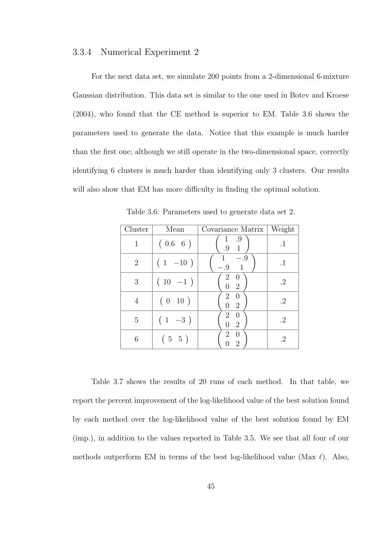
3.3.4 Numerical Experiment 2
For the next data set, we simulate 200 points from a 2-dimensional 6-mixture
Gaussian distribution. This data set is similar to the one used in Botev and Kroese
(2004), who found that the CE method is superior to EM. Table 3.6 shows the
parameters used to generate the data. Notice that this example is much harder
than the first one; although we still operate in the two-dimensional space, correctly
identifying 6 clusters is much harder than identifying only 3 clusters. Our results
will also show that EM has more difficulty in finding the optimal solution.
Table 3.6: Parameters used to generate data set 2.
Cluster Mean Covariance Matrix Weight
1(
0.6 6) (
1 .9.9 1
).1
2(
1 −10) (
1 −.9−.9 1
).1
3(
10 −1) (
2 00 2
).2
4(
0 10) (
2 00 2
).2
5(
1 −3) (
2 00 2
).2
6(
5 5) (
2 00 2
).2
Table 3.7 shows the results of 20 runs of each method. In that table, we
report the percent improvement of the log-likelihood value of the best solution found
by each method over the log-likelihood value of the best solution found by EM
(imp.), in addition to the values reported in Table 3.5. We see that all four of our
methods outperform EM in terms of the best log-likelihood value (Max `). Also,
45

the worst solution (Min `) is much better than the worst solution found by EM,
and the variance of the solutions is smaller. To be fair, we also see that the time
for convergence increases drastically for the global optimization methods. However,
this may be a fair price for obtaining significantly better solutions.
Table 3.7: Simulation results on data set 2 based on 20 runs.
Algorithm Max ` Min ` Mean ` S.E.(`) imp. iters Avg timeEM -956.34 -1060.9 -981.25 5.71 - 23.20 0.26
CE-EM -947.02 -1019.0 -975.78 4.64 0.97% 257.65 55.50CE-CD -946.98 -999.83 -967.73 4.08 0.98% 249.35 56.65
MRAS-EM -947.08 -1018.4 -979.81 4.10 0.97% 217.15 47.23MRAS-CD -947.12 -997.76 -967.92 3.28 0.96% 227.85 58.06
Figure 3.9 shows what can be gained using a global optimization method. In
that figure, we see the best solution found by EM versus the best solution found by
MRAS-CD. Note that based on Table 3.7 alone, the difference does not appear large
(-956.34 for EM versus -947.12 for MRAS-CD, an improvement of less than 1%).
However, Figure 3.9 indicates that MRAS-CD identifies the 6 clusters much better
than EM. In fact, while both methods correctly identify the bottom 3 clusters, EM
has a hard time distinguishing between the upper 3 clusters. While EM overesti-
mates the first cluster, it underestimates the other two. The reason for this poor
performance is that the upper 3 clusters are not well separated and EM commits
too soon on a final solution. On the other hand, MRAS-CD explores the solution
space better and spends a longer time doing so. Only after a thorough exploration
of the solution space, MRAS-CD settles on a final solution which also is the true
solution.
46
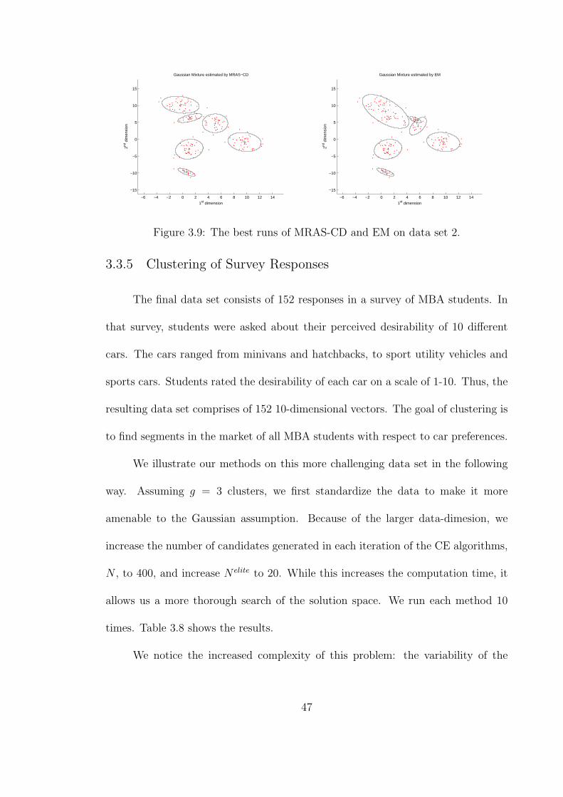
−6 −4 −2 0 2 4 6 8 10 12 14
−15
−10
−5
0
5
10
15
1st dimension
2nd d
imen
sion
Gaussian Mixture estimated by MRAS−CD
−6 −4 −2 0 2 4 6 8 10 12 14
−15
−10
−5
0
5
10
15
1st dimension
2nd d
imen
sion
Gaussian Mixture estimated by EM
Figure 3.9: The best runs of MRAS-CD and EM on data set 2.
3.3.5 Clustering of Survey Responses
The final data set consists of 152 responses in a survey of MBA students. In
that survey, students were asked about their perceived desirability of 10 different
cars. The cars ranged from minivans and hatchbacks, to sport utility vehicles and
sports cars. Students rated the desirability of each car on a scale of 1-10. Thus, the
resulting data set comprises of 152 10-dimensional vectors. The goal of clustering is
to find segments in the market of all MBA students with respect to car preferences.
We illustrate our methods on this more challenging data set in the following
way. Assuming g = 3 clusters, we first standardize the data to make it more
amenable to the Gaussian assumption. Because of the larger data-dimesion, we
increase the number of candidates generated in each iteration of the CE algorithms,
N , to 400, and increase N elite to 20. While this increases the computation time, it
allows us a more thorough search of the solution space. We run each method 10
times. Table 3.8 shows the results.
We notice the increased complexity of this problem: the variability of the
47

Table 3.8: Simulation results on the survey data set based on 10 runs.
Algorithm Max ` Min ` Mean ` S.E.(`) imp. iters Avg timeEM -1622.1 -1942.2 -1797.6 28.20 - 13.6 0.14
CE-EM -1623.4 -1857.2 -1694.8 19.88 -0.08% 151.8 90.50CE-CD -1300.6 -1809.9 -1599.3 37.85 19.83% 280.0 265.62
MRAS-EM -1329.9 -1955.5 -1709.6 39.10 18.01% 117.4 68.45MRAS-CD -1435.5 -1886.1 -1620.4 32.87 11.50% 268.4 297.91
solutions is larger and so is the average computing time. However, we also notice the
much larger gains of our methods compared to EM: for three out of the four methods,
the improvement over EM ranges between 10% and 20%. Only CE-EM fails to
produce a better solution than EM. One reason for this underperformance may be
the close link to EM via the covariance-updating procedure, which may not allow
enough flexibility to explore the entire solution space. We also note that since we
increased the number of candidates generated per iteration, the computational time
difference between our methods and EM is now even larger. EM is approximately 3
orders of magnitude faster than the new methods in this experiment.
In order to gauge what can be gained from the global optimum, consider the
graph in Figure 3.10, which depicts the best set of clusters obtained by each of the
two methods, with the data projected onto the first two principal components. We
can see that the best solution obtained by MRAS-CD (left panel) separates the data
much better into 3 distinct clusters than the best solution obtained by EM (right
panel). In particular, in the left panel the cluster means are much better separated,
as are the cluster shapes (i.e., the corresponding covariance matrices). The clusters
in the left panel span the data set without the amount of overlap seen in the right
48
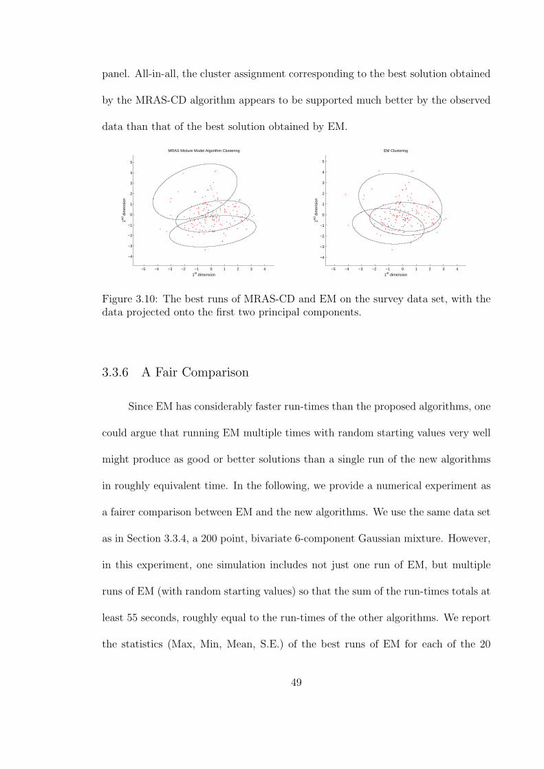
panel. All-in-all, the cluster assignment corresponding to the best solution obtained
by the MRAS-CD algorithm appears to be supported much better by the observed
data than that of the best solution obtained by EM.
−5 −4 −3 −2 −1 0 1 2 3 4
−4
−3
−2
−1
0
1
2
3
4
5
1st dimension
2nd d
imen
sion
MRAS Mixture Model Algorithm Clustering
−5 −4 −3 −2 −1 0 1 2 3 4
−4
−3
−2
−1
0
1
2
3
4
5
1st dimension
2nd d
imen
sion
EM Clustering
Figure 3.10: The best runs of MRAS-CD and EM on the survey data set, with thedata projected onto the first two principal components.
3.3.6 A Fair Comparison
Since EM has considerably faster run-times than the proposed algorithms, one
could argue that running EM multiple times with random starting values very well
might produce as good or better solutions than a single run of the new algorithms
in roughly equivalent time. In the following, we provide a numerical experiment as
a fairer comparison between EM and the new algorithms. We use the same data set
as in Section 3.3.4, a 200 point, bivariate 6-component Gaussian mixture. However,
in this experiment, one simulation includes not just one run of EM, but multiple
runs of EM (with random starting values) so that the sum of the run-times totals at
least 55 seconds, roughly equal to the run-times of the other algorithms. We report
the statistics (Max, Min, Mean, S.E.) of the best runs of EM for each of the 20
49

simulations.
Table 3.9: Simulation results on data set 2 based on 20 runs for the new algorithms,and 20 sets of multiple runs of EM compliling a total run-time of at least 55 seconds.
Algorithm Max ` Min ` Mean ` S.E.(`) Avg timeEM -946.98 -958.24 -951.04 1.53 55.69
CE-EM -947.02 -1019.0 -975.78 4.64 55.50CE-CD -946.98 -999.83 -967.73 4.08 56.65
MRAS-EM -947.08 -1018.4 -979.81 4.10 47.23MRAS-CD -947.12 -997.76 -967.92 3.28 58.06
Table 3.9 contains the results of the fair comparison simulations. Running EM
multiple times for roughly equivalent times compared to the proposed algorithms
produces the global optimum on multiple trials. Moreover, the minimum and mean
likelihood values across the 20 trials are an improvement over the proposed algo-
rithms. This experiment shows that for the current state of the proposed algorithms
and for this particular data set, the algorithms have slightly poorer overall perfor-
mance on average as multiple runs of EM for equivalent time. However, optimizing
the proposed algorithms for speed would reduce the run-times of the algorithms, thus
lessening the ability of EM to find the global optimum alloting the same run-times.
3.3.7 Does the Global Optimum “Matter”?
One question that comes to mind when considering local, sub-optimal solutions
is whether the global optimum really matters. That is, does knowledge of the global
solution make a difference in practice or is the difference merely academic. In the
following, we conduct a numerical experiment to answer this question.
In this numerical experiment, we test how the global optimization clustering
50

algorithms perform in relation to EM, not only gauging the goodness of fit by the
log-likelihood values, but also using the resulting mixture distribution to classify a
select subset of the data points according to the computed clusters. Specifically, we
take simulated data, of which we know the underlying parametric distribution as
well as the true cluster membership of each data point, and randomly select 70% of
the data and declare it the training set. We call the remaining 30% of the data the
test set.
We use the EM, CE-EM, CE-CD, MRAS-EM, and MRAS-CD algorithms to
estimate the clusters from the training set, which is held constant throughout the ex-
periment. After we cluster the training set, we use the computed cluster parameters
to compute the posterior probabilities of the test set, according to Equation (2.1).
Each posterior probability, τij, represents the probability that test point i belongs
to cluster j. Because we simulated the data, we know the true cluster membership
of each data point. We refer to the true membership as τ ∗ij, which we set to 1 if test
point i was simulated from cluster j, and 0 otherwise. So, we can refer to τ ∗i as the
true g-dimensional cluster membership vector for the ith test point.
To quantify how well the the clustering algorithms perform, we look at how
the estimated posterior probailities τij compare with the true values τ ∗ij. One way we
do so is to assign each test point yi to cluster j∗, where j∗ = argmaxj τij. Then, we
count the number of correctly assigned test points and compute the corresponding
empirical probabililty p.
Another way is to compute the norm of the difference of the two vectors τi and
τ ∗i , effectively computing a distance between the estimated and the true vectors. We
51

compute the average L2 norm for the data points, which we refer to as D, via:
D =
∑ni=1 ‖τi − τ ∗i ‖
n.
We simulate 500 data points from the bivariate Gaussian mixture distribution
seen in Table 3.6, and designate 350 of them as the training set, and the remaining
150 as the test set. We then apply each algorithm 20 times. Table 3.10 contains
the simulation results of the 20 runs. We report the mean and standard errors of
the following values: the resulting log-likelihood values (`), the proportion correctly
assigned to the true membership (p), and the average norm (D).
Table 3.10: Simulation results on data set 1 based on 20 runs.
Algorithm Mean ` S.E.(`) p√p(1− p) Mean D S.E.(D)
EM -1759.3 9.31 .810 .0231 .281 .0327CE-EM -1749.2 8.34 .808 .0198 .282 .0303CE-CD -1721.3 5.66 .911 .0151 .136 .0223
MRAS-EM -1730.9 4.10 .861 .0168 .201 .0237MRAS-CD -1726.1 4.66 .895 .0150 .158 .0221
The results in Table 3.10 indicate that, on average, EM produces solutions
with a log-likelihood value of −1759.3, and a standard error of 9.31. On the other
hand, all of our four proposed algorithms perform better with average log-likelihood
values higher than that of EM. In particular, CE-CD performs the best in this
experiment, with an average log-likelihood value of −1721.3. Additionally, the pro-
posed algorithms all produce solutions with lower variability than EM, as evidenced
by the smaller standard errors of the likelihood values. EM correctly classifes the
test points in this experiment with estimated probability p = .810, and a standard
error of .0231. While the classification rate of CE-EM is marginally lower than EM
52

at .808, the other three algorithms perform significantly better than EM. The two
methods that utilize the Cholesky decomposition perform the best, with CE-CD
and MRAS-CD correctly classifying 91.1% and 89.5% of the data, an improvement
of about 10% over EM. All four proposed algorithms also produce solutions that
classify with significantly lower variability than EM, as seen by the lower standard
errors of p. Looking at the average norm D, again CE-EM has a slightly poorer
performance than EM, whose average norm is .281. Analogous to the results for p,
the other three algorithms exhibit much better performance than EM, with CE-CD
performing the best with an average of .136. Again, all four algorithms have lower
standard errors for the computed norms than EM.
From Table 3.10, we can conclude that the better likelihood values found by
CE-CD, MRAS-EM, and MRAS-CD directly translate into better clustering per-
formance on the test set. The only exception is CE-EM, which, despite marginally
better (average) solutions, does not cluster the data any better than EM. It is gen-
erally also revealing that the CD-based global optimization methods (CE-CD &
MRAS-CD) perform better than the ones based on EM. An explanation for this
phenomenon is the de-coupling of mean and variance estimation in the CD-based
methods. While CE-EM and MRAS-EM use the EM updates for estimating the co-
variance matrices (which are not independent of the estimated means), CE-CD and
MRAS-CD update the covariance matrices independently of the cluster means and
cluster proportions. This increased flexibility may lead to an improved exploration
of the solution space and, consequently, to better clustering performance.
53

3.4 Discussion
In this chapter we introduced several new methods to find globally optimal so-
lutions for model-based clustering problems. Numerical experiments indicate that,
although they are more computationally intensive than the classical EM, the pro-
posed algorithms perform better on average than EM. In fact, the experiments show
that unlike EM, the new methods are relatively insensitive to the starting points. In
addition to cross-validating the results using classification techniques as in Section
3.3.7, calculating the likelihood ratio chi-square significance is another way to test
the significance of improved solutions for mixture models.
The computational costs of the new methods are orders of magnitudes greater
than the EM algorithm, and in some cases, the additional gains in performance are
marginal, so an important research avenue to pursue would be a characterization
of when the new methods are most effective. Clearly, higher-dimensional problems
offer one opportunity, as demonstrated by the MBA survey example example, but
even so, it would be worthwhile to determine which properties of the problem lead to
more local solutions. Characterizing how the run-time complexity of the proposed
algorithms changes with respect to problem size would also be an important factor
for determining when the algorithms are most effective.
Another potential avenue of future work for these algorithms would be to
generalize the objective function in order to find the best clustering across all val-
ues of g. One approach for doing so would be to wrap a suitable model-selection
criterion around the algorithms for varying values of g. Other approaches might
54

include incorporating some sort of hierarchical clustering scheme into the proposed
algorithms.
Other extensions to our work include application of global optimization meth-
ods to general mixture models, as well as other data mining algorithms such as
neural networks. Both CE and MRAS provide a natural framework for these op-
timization problems, and tailoring CE and MRAS to them could result in better
global solutions. Also, as the EM algorithm forms the basis for many supervised
and unsupervised learning methods, application of these methods to that field are
worth investigating.
55

Chapter 4
Global Convergence of Gaussian Mixture Models with MRAS
4.1 Motivation
Because the likelihood function of Gaussian mixture models typically has a
large number of local maxima, finding the global maximum can be a difficult task.
Many optimization methods only guarantee convergence to a local optimum, and
are not necessarily concerned with systematically finding the global optimum. In
this chapter we discuss a method specifically designed to find the global optimum.
The method was first introduced in the field of operations research and is referred
to as Model Reference Adaptive Search.
Model Reference Adaptive Search (MRAS) is a method that was first proposed
in the field of operations research and is designed to attain globally optimal solutions
to general multi-extremal continuous optimization problems (Hu et al., 2007). As
discussed in Chapter 3, MRAS produces estimates to optimization problems by iter-
atively generating candidate solutions in each iteration from a parametric sampling
distribution. The candidates are all scored according to an objective function, and
the highest scoring candidates are used to update the parameters of the sampling
distribution by minimizing the Kullback-Leibler (KL) divergence between the sam-
pling distribution and the current reference model. Due to the choice of the reference
model sequence, the updating scheme of MRAS leads to a more general framework
56

than the CE method, and allows for rigorous analysis of theoretical convergence (Hu
et al., 2007).
Many global optimization algorithms that perform well empirically have no
theoretical convergence proofs. A good number of these algorithms are ad-hoc or
based on heuristics that do not allow for a rigorous mathematical investigation of
their convergence properties. In particular, these approaches lack a built-in mech-
anism to systematically escape from locally optimal solutions. For instance, the
methods we discuss in Chapter 1 that are designed to globally optimize the likeli-
hood function of Gaussian mixture models are not theoretically globally convergent.
In contrast, in this chapter we prove global convergence of the MRAS-CD algorithm
to the global optimum of Gaussian mixtures. To the best of our knowledge, this
is the first mixture analysis algorithm that has provable global convergence. In
addition to providing theoretical justification that the algorithm is not merely an
ad-hoc heuristic, the convergence proof also gives insight into the performance of
the algorithm.
The rest of the chapter begins with an explanation of MRAS in general, as
well as some details on its convergence proof in Section 4.2. We discuss the MRAS-
CD algorithm and prove its convergence to the global optimum of the likelihood
function Gaussian mixture models in Section 4.3. We summarize the findings in the
discussion in Section 4.4.
57

4.2 Model Reference Adaptive Search
Model Reference Adaptive Search (MRAS) is a global optimization tool that
estimates the global optimum by generating candidate solutions from a parametric
sampling distribution in each iteration. Hu et al. (2007) introduce MRAS as a
method that produces solutions to the following global optimization problem:
x∗ ∈ argmaxx∈χ
H(x), χ ⊆ <n.
MRAS achieves this goal by utilizing a sequence of intermediate reference distribu-
tions on the solution space to guide the parameter updates.
The basic methodology of MRAS can be described as follows. In the kth iter-
ation, we generate Nk candidate solutions, X1, X2, ..., XNk, according to a sampling
distribution g( · ; Υ(k)), where Υ(k) represents the sampling parameters of the kth
iteration. After sampling the candidates, we score them according to the objective
function, i.e., we compute the objective function value H(Xi) for each candidate
Xi. We then obtain an elite pool of candidates by selecting the top ρ-percentile
scoring candidates. These elite candidates are used to update the parameters of the
sampling distribution for the next iteration. An outline of MRAS is given in Figure
4.1.
In MRAS, the value of the percentile ρ changes over the course of the algorithm
to ensure that the current iteration’s candidates improve upon the candidates in the
previous iteration. Let the lowest objective function score among the elite candidates
in any iteration k be denoted as γk. We introduce a parameter ε, a very small positive
number, to ensure that the increment in the γk sequence is strictly bounded below.
58

Result: Return highest-scoring estimate for x∗
Initialize Υ(0).1
k ← 0.2
repeat3
Generate Nk i.i.d. candidate vectors X1, ..., XNkfrom the sampling4
distribution g( · ; Υ(k)).Compute the objective function values H(X1), H(X2), ..., H(XNk
).5
Select the elite candidates by taking the top scoring ρ-percentile6
candidate vectors.Compute the updated MRAS sampling parameters Υ(k+1) via (4.1)7
using the elite candidates.k ← k + 1.8
until Stopping criterion is met.9
Figure 4.1: MRAS Outline
If γk < γk−1+ε, increase ρ until γk ≥ γk−1+ε, effectively reducing the number of elite
candidates. If, however, no such percentile ρ exists, then the number of candidates is
increased in the next iteration by a factor of α (where α > 1), such that Nk+1 = αNk.
The sampling parameters are then updated as follows:
Υ(k+1) := argmaxΥ∈Θ
1
Nk
Nk∑i=1
[S(H(Xi))]k
g(Xi; Υ(k))IH(Xi)≥γk+1 ln g(Xi; Υ), (4.1)
where S : < → <+ is a strictly increasing function to account for cases where
the objective function value H(X) is negative for a given X, and I· denotes the
indicator function such that:
IA :=
1, if event A holds,
0, otherwise.
The sampling distribution g in MRAS is generally chosen from the natural
exponential family. We choose to sample candidate solutions from the Gaussian
distribution for our implementation, such that Υ = (ξ,Ω), where ξ and Ω are the
mean and covariance matrix of the MRAS sampling distribution, respectively. The
59

main idea of MRAS is that the sampling parameters will converge to a degenerate
distribution centered on the optimal solution; i.e., the sequence of means ξ(0), ξ(1), ...
will converge to the optimal vector X∗, representing the optimal solution x∗, as
the sequence of the sampling covariance matrices Ω(0),Ω(1), ... converges to the zero
matrix. Table 4.1 provides a list of the mixture model parameters and the MRAS
parameters.
Table 4.1: List of the model and MRAS parameters.
Mixture Model parameters MRAS parameters
n = number of data points Υ(k) = sampling parameters in kth
yi = ith data point iterationp = dimension of data g( · ; Υ(k)) = sampling densityg = number of mixture components Nk = number of candidates in kth
πj = weight of jth mixture compo- iterationnent Xi = candidate vectorψj = probability distribution para- ρ = elite candidate percentilemeters of jth component γk = lowest objective score of eliteψj = probability distribution para- candidates in kth iterationmeters of jth component λ = sampling weightfj( · ;ψj) = probability density ofjth component
S : < → <+ = strictly increasingfunction
θ = model parameters to estimate X∗ = candidate vector representingθ∗ = model parameters that repre- the global optimumsent the global optimum ε = lower bound on the increase of`(y, θ) = log-likelihood function each γk
µj = Gaussian mixture mean vector ξ(k) = Gaussian sampling mean vec-Σj = Gaussian mixture covariance tormatrix Ω(k) = Gaussian sampling covari-
ance matrixχ = constrained domain for candi-date vectorsH( · ) = objective functionΘ = constrained domain for sam-pling parameters
While MRAS is generally very versatile, applying it to the mixture model
60

context is not straightforward. Part of the reason is that the mixture model requires
simulation of candidate solutions that satisfy the mixture model constraints. In the
following, we propose a solution via the Cholesky decomposition in order to assure
an efficient implementation of MRAS.
4.2.1 Global Convergence of MRAS
In this section we discuss the global convergence properties of MRAS mixture
model algorithm in the finite mixture model problem. We must first revert to the
general MRAS framework, where Hu et al. (2007) provide a convergence proof of
MRAS to the globally optimal solution when using a sampling distribution g( · ; Υ)
that belongs to the exponential family. Before we discuss the theorem, we provide
the definition of the exponential family of distributions, as well as some required
assumptions for the theorem.
Definition 4.1 A parameterized family of p.d.f.’s g( · ; Υ),Υ ∈ Θ ⊆ <m on χ
is said to belong to the exponential family if there exists functions h : <n → <,Γ :
<n → <m, and K : <m → < such that
g(x; Υ) = expΥT Γ(x)−K(Υ)h(x), ∀Υ ∈ Θ,
where K(Υ) = ln∫
x∈χexpΥT Γ(x)h(x)dx.
The following assumptions are referenced in the statement of Theorem 4.1.
Assumptions:
A1. For any given constant ξ < H(x∗), the set x : H(x) ≥ ξ ∩ χ has a
strictly positive Lebesgue measure.
61

A2. For any given constant δ > 0, supx∈AδH(x) < H(x∗), where Aδ : = x :
‖x − x∗‖ ≥ δ ∩ χ and the supremum over the empty set is defined to
be −∞.
A3. There exists a compact set Πε such that x : H(x) ≥ H(x∗) − ε ∩
χ ⊆ Πε. Moreover, g(x; Υ(0)) is bounded away from zero on Πε, i.e.,
g∗ = infx∈Πε g(x; Υ(0)) > 0.
A4. The parameter vector Υ(k) computed in (4.1) is an interior point of Θ
for all k.
In Theorem 4.1, Hu et al. (2007) show global convergence of MRAS to the
optimal solution x∗ when using the multivariate Gaussian sampling distribution. As
the number of iterations tends to infinity, the sampling distribution tends toward a
degenerate distribution centered on the optimal solution x∗.
Theorem 4.1 If multivariate Gaussian p.d.f.’s are used in MRAS, i.e.,
g(X; ξ(k),Ω(k)) =1√
(2π)n|Ω(k)| exp
(−1
2(X − ξ(k))T (Ω(k))−1(X − ξ(k))
),
ε > 0, α > (βS∗)2, and Assumptions A1, A2, A3, and A4 are satisfied, then
limk→∞
ξ(k) = x∗, and limk→∞
Ω(k) = 0n×n w.p. 1
4.3 MRAS algorithm for Gaussian Mixture Models
As pointed out above, MRAS requires, in every iteration, the simulation of
candidate solutions from within the parameter space. In the Gaussian mixture
62

model, these candidate solutions must include the mixture weights π = (π1, ..., πg)
and the probability distribution parameters ψj = (µj,Σj) for j = 1, ..., g, where µj
is the mean vector and Σj is the covariance matrix of the jth component. Simulat-
ing covariance matrices is involved, since they need to be positive definite. Naive
approaches (e.g., via simulating matrices randomly and consequently selecting only
those that are positive definite) can be extremely inefficient. In Chapter 3 the
MRAS-CD algorithm was introduced as an algorithm utilizes updating the Cholesky
factorization of a covariance matrix to efficiently simulate s.p.d. covariance matrices.
that applied MRAS to Gaussian mixture models updated the covariance matrices of
iteratively. In this chapter, we look more closely at one of those algorithms, namely
MRAS-CD. and we proposed several algorithm. In th following, we propose a new
method to simulate positive definite covariance matrices for the MRAS mixture
model algorithm. This method relies on the Cholesky decomposition. Recall the
following theorem (see e.g., Thisted, 1988) regarding the Cholesky decomposition of
a symmetric positive definite matrix:
Theorem 4.2 A real, symmetric matrix A is symmetric positive definite (s.p.d.)
if and only if it has a Cholesky decomposition such that A = UTU , where U is a
real-valued upper triangular matrix.
Because covariance matrices are s.p.d., each covariance matrix has a corre-
sponding Cholesky factorization U . Therefore, one way to stochastically generate
covariance matrices in the MRAS mixture model is to generate the components
of the U matrix from the Cholesky decomposition instead of the components of
63

the covariance matrix Σ directly. Note that only the p(p + 1)/2 upper right-hand
components of U must be generated for each p × p covariance matrix (all other
components are necessarily zero). Then the covariance matrix can be constructed
from the simulated Cholesky factors, ensuring that the covariance matrix is s.p.d.
One potential problem with this method is that the Cholesky factorization for
a symmetric positive definite matrix is not unique. For a Cholesky factorization
U of Σ, we can multiply any subset of rows of U by −1 and obtain a different
Cholesky factorization of the same Σ. Thus, there is not a unique global optimum
in the MRAS mixture model algorithm. However, in their discussion of parame-
terizations of positive definite matrices, Pinheiro and Bates (1996) note that if the
diagonal elements of the Cholesky factorization U are required to be positive, then
the Cholesky factorization U is unique. Thus, by restricting the diagonal elements
of U to be positive, we can circumvent the uniqueness problem of the Cholesky
factorization mentioned above. We therefore choose to construct the covariance
matrices in the MRAS mixture model algorithm by sampling the diagonal compo-
nents of U from a truncated Gaussian distribution (accepting all positive values),
and subsequently computing the covariance matrix Σ = UTU .
MRAS can now be applied to the estimation of Gaussian mixtures in the fol-
lowing way. We first sample candidate solutions Xi that correspond to the set of
mixture parameters θ = (µj,Σj, πj)gj=1, where the covariance matrices are repre-
sented by their corresponding Cholesky factorizations mentioned above. We then
score each candidate with the log-likelihood function, and use the best-scoring can-
didates to update the sampling distribution. The goal is to obtain the optimal
64

solution X∗ containing the mixture means, Cholesky factorizations, and weights of
the global maximum likelihood estimate θ∗ = (µ∗j ,Σ∗j , π
∗j )
gj=1. We provide the MRAS
mixture model algorithm in Figure 4.2. Note that the MRAS parameter λ is a small
constant which assigns a probability to sample from the initial sampling distribution
g( · ; Υ(0)) in any subsequent iteration. Also, g( · ; ξ,Ω) is the multivariate Gaussian
density, i.e.,
g(X; ξ,Ω) =1√
(2π)p|Ω| exp
(−1
2(X − ξ)T Ω−1(X − ξ)
),
where |Ω| denotes the determinant of the matrix Ω.
The stopping criterion for the MRAS mixture model algorithm that we use is to
stop when the increase of the best log-likelihood value over k iterations falls below
a specified tolerance.
4.3.1 Preventing Degenerate Solutions
As mentioned in Section 3.3.1, maximizing the log-likelihood function in the
Gaussian mixture model can lead to unbounded solutions, if the parameter space
is not properly constrained. Therefore, we choose to constrain the MRAS mixture
model algorithm generates a covariance matrix that violates the constraint given by
Equation (3.3), we discard the candidate and re-generate a new one.
65

Data: Data points y1, y2, ..., yn
Result: Return highest-scoring estimate for X∗.Initialize ξ(0) and Ω(0).1
k ← 0.2
repeat3
Generate Nk i.i.d. candidate vectors X1, ..., XNkfrom the sampling4
distribution g( · ; ξ(k),Ω(k)) := (1− λ)g( · ; ξ(k),Ω(k)) + λg( · ; ξ(0),Ω(0)).Compute the log-likelihoods values `(y,X1), `(y,X2), ..., `(y,XNk
).5
Select the elite candidates by taking the top scoring ρk−1-percentile6
candidate vectors, and define γk(ρk) as the ρk-percentile log-likelihoodscore obtained of all candidates in iteration k.if k = 0 or γk(ρk) ≥ γk + ε
2then7
γk+1 ← γk(ρk), ρk+1 ← ρk, and Nk+1 ← Nk.8
else9
find the largest ρ ∈ (ρk, 100) such that γk(ρ) ≥ γk + ε2.10
if such a ρ exists then11
γk+1 ← γk(ρ), ρk+1 ← ρ, and Nk+1 ← Nk,12
else13
γk+1 ← γk, ρk+1 ← ρk, and Nk+1 ← αNk.14
end15
end16
Update the sampling parameters according to:17
ξ(k+1) ←∑Nk
i=1S(`(y,Xi))
kXi
g(Xi,ξ(k),Ω(k))I`(y,Xi)≥γk+1∑Nk
i=1S(`(y,Xi))k
g(Xi,ξ(k),Ω(k))I`(y,Xi)≥γk+1
, (4.2)
Ω(k+1) ←∑Nk
i=1S(`(y,Xi))
k(Xi−ξ(k+1))(Xi−ξ(k+1))T
g(Xi,ξ(k),Ω(k))I`(y,Xi)≥γk+1∑Nk
i=1S(`(y,Xi))k
g(Xi,ξ(k),Ω(k))I`(y,Xi)≥γk+1
. (4.3)
k ← k + 1.18
until Stopping criterion is met.19
Figure 4.2: MRAS Mixture Model Algorithm
4.3.2 Proving Global Convergence of the MRAS Mixture Model Al-
gorithm
In order to show that Theorem 4.1 applies to the MRAS mixture model al-
gorithm algorithm, we must show that Assumptions A1, A2, A3, and A4 hold true
66

in the maximization of the likelihood function of the mixture density. So, for our
purposes, the objective function H(x) discussed in the general MRAS framework is
the log-likelihood of the mixture density:
`(y, θ) =n∑
i=1
log
g∑j=1
πjfj(yi;µj,Σj).
In the MRAS mixture model algorithm, we are estimating the vectorX∗ representing
the optimal means, weights, and Cholesky factorizations of the covariance matrices,
i.e., the vector X∗ representing the optimal solution θ∗ = (µ∗i ,Σ∗i , π
∗i )
gi=1. Therefore,
we are trying to solve the optimization problem:
X∗ ∈ argmaxX∈χ
`(y,X).
Before we prove the global convergence of the MRAS mixture model algorithm,
we first provide the following useful lemmas. Lemma 4.1 shows that a continuous
function that is bounded above and possesses a unique optimal maximizer on a
constrained space χ ∈ <n satisfies Assumption A1.
Lemma 4.1 For a continuous function H(x), x ∈ χ ∈ <n, where H is bounded
above and there exists a unique optimal maximizer x∗ s.t. H(x) < H(x∗), ∀x 6= x∗,
then ∀ξ < H(x∗), the set x : H(x) ≥ ξ has strictly positive Lebesgue measure, and
thereby Assumption A1 is satisfied.
Proof: Choose ξ < H(x∗) and let ε = H(x∗)−ξ > 0. By continuity of H, ∃δ > 0 s.t.
∀x ∈ x : ‖x− x∗‖ < δ, then |H(x)−H(x∗)| < ε. By rewriting the left- and right-
hand sides of the inequality, we see that H(x∗)−H(x) < H(x∗)− ξ, i.e., ξ < H(x),
∀x ∈ x : ‖x− x∗‖ < δ. Since the set x : ‖x− x∗‖ ≤ δ2 ⊆ x : H(x) ≥ ξ, then
m (x : H(x) ≥ ξ) ≥ m(x : ‖x− x∗‖ ≤ δ
2) > 0. 2
67

Lemma 4.2 gives an inequality relating the determinants of two positive definite
n×n matrices with the determinant of their convex combination (see e.g., Horn and
Johnson, 1990).
Lemma 4.2 For positive definite n× n matrices A and B,
det (αA+ (1− α)B) ≥ (detA)α(detB)1−α, where α ∈ (0, 1).
In Lemma 4.3 we extend the statement of Lemma 4.2 to a convex combination
of an arbitrary number of positive definite n×n matrices. In the proof, we make use
of two properties of positive definite matrices: for positive definite matrices A,B,
and scalar α > 0, then αA and A + B are both positive definite as well (Johnson,
1970).
Lemma 4.3 For positive definite n× n matrices Aj, j = 1, ..., k,
det
(k∑
j=1
αjAj
)≥
k∏j=1
(detAj)αj ,
for any set of αjkj=1 s.t. αj > 0 and∑k
j=1 αj = 1.
Proof: We prove this lemma by induction.
i. Base case: k = 2, shown by Lemma 4.2.
ii. Assuming the lemma holds for k, we show it holds for k + 1, i.e., for any set
αjk+1j=1 s.t. αj > 0 and
∑k+1j=1 αj = 1, then,
det
(k+1∑j=1
αjAj
)≥
k+1∏j=1
(detAj)αj .
68

Define αj =αj
1−αk+1, for j = 1, ..., k. Thus,
∑kj=1 αj = 1 and the induction
assumption can be applied to A1, ..., Ak for this set of αjkj=1. Then,
det
(k+1∑j=1
αjAj
)= det
(k∑
j=1
αjAj + αk+1Ak+1
)
= det
((1− αk+1)
k∑j=1
αjAj + αk+1Ak+1
)
≥[det
(k∑
j=1
αjAj
)]1−αk+1
(detAk+1)αk+1 (by Lemma 2)
≥[
k∏j=1
(detAj)αj
]1−αk+1
(detAk+1)˜αk+1
(by induction
assumption
)
=
[k∏
j=1
(detAj)αj
](detAk+1)
αk+1
=k+1∏j=1
(detAj)αj .
Therefore, we have shown by induction that the statement of the lemma is true. 2
Constraining the parameter space is necessary for the proof of the MRAS
mixture model algorithm convergence theorem. As mentioned in Section 3.3, we
must place additional constraints on the parameter space in order to prevent de-
generate clusters and an unbounded log-likelihood value. Specifically, these con-
straints are |UTj Uj| ≥ c > 0, j = 1, ..., g, i.e., bounding the generalized variances
of the covariance matrices below. We simplify this constraint by relying on a con-
venient property of determinants of positive definite matrices: for positive defi-
nite A,B, detAB = detA detB. So, for the Cholesky decomposition Σ = UTU ,
|Σ| = |UT ||U | = |U |2. Equivalently, we write |U | ≥ √c. Since U is an upper-
69

triangular matrix, |U | is equal to the product of its diagonal elements. So, the
constraint |UTU | ≥ c can be written as∏p
i=1 Uii ≥√c.
One condition that is necessary for satisfying Assumption A2 is that the op-
timal candidate solution X∗ be unique. By restricting the diagonal components of
the Cholesky factorization U to be positive, its correponding covariance matrix Σ
is unique. However, for a given optimal solution, any permutation of the cluster
labels will result in an equivalent log-likelihood value to the problem, resulting in
g! optimal solutions and therefore a non-indentifiable formulation. To avoid this
problem, we add the following constraint to the problem:
µ1(1) ≤ µ2(1) ≤ µ3(1) ≤ ... ≤ µg(1),
where µi(1) represents the 1st mean component of the ith cluster. Although the
inequalities in this constraint are not strict, the probability of multiple mean com-
ponents of continuous random data being equal is zero. Therefore, this constraint
mandates a unique ordering of the mixture components of θ∗ w.p. 1 for continuous
random data, resulting in a unique optimal candidate solution X∗ to the MRAS
Gaussian mixture model algorithm.
To allow us to prove convergence, we choose to bound the candidate means
within a compact space based on the observed data set. In particular, we define
ymin as the minimum value over all components of the data points y1, ..., yn. That
is, ymin(i) = minj=1,...,n yj(i). Similarly, we define ymax as the maximum value over
all components of the data points, i.e., ymax(i) = maxj=1,...,n yj(i). We note that
bounding the candidate mean components by ymin and ymax is not an unreasonable
70

constraint; clearly, the means of the optimal clusters will not lie outside the range
of the data.
We also place constraints on the components of the Cholesky factorizations
when we generate the candidate vectors. We first calculate the sample variance
of the data set, V ar(y1, y2, ..., yn), and then choose the maximum across all p
components, i.e., Vmax = maxi=1,...,p V ar(y1, y2, ..., yn). And so, Vmax represents an
upper bound for the variance component of any cluster. Constraining the diagonal
components of the Cholesky factorizations within the bounds [0, Vmax] and the off-
diagonal non-zero components within [−Vmax, Vmax] suffices, as the global optima
will undeniably satisfy these constraints.
Therefore, the solution space with all of the necessary constraints is given by
the following:
χ =
µj ∈ [ymin, ymax], j = 1, ..., g
s.t. µ1(1) ≤ µ2(1) ≤ ... ≤ µg(1)
Uj(ii) ∈ [0, Vmax], j = 1, ..., g; i = 1, ..., p
s.t.∏p
i=1 Uj(ii) ≥√c > 0, j = 1, ..., g
Uj(ik) ∈ [−Vmax, Vmax], j = 1, ..., g; i = 1, ..., p− 1;
k = i+ 1, ..., p
πj ∈ [0, 1], j = 1, ..., g
s.t.∑g
j=1 πj = 1
(4.4)
The number of parameters that we are estimating, namely the means, weights,
and the upper-triangular entries of the Cholesky factorization (all other components
71

are necessarily zero) for each cluster, is d := g (p+1)(p+2)2
, so we can consider the space
χ to be d-dimensional. The MRAS sampling parameters Υ = (ξ,Ω) belong to the
space Θ, where Θ = ξ ∈ χ, Ω is s.p.d..
Lemma 4.4 The subspace χ ⊆ <d is compact.
Proof: For any vector X ∈ χ, we note that all components of X are bounded
as described in (4.4). We now show that the space χ is closed. The constraints
that bound the space clearly constitute a closed subspace in <d. The remaining
constraints, namely µ1(1) ≤ µ2(1) ≤ ... ≤ µg(1),∏p
i=1 Uj(ii) ≥√c for j = 1, ..., g,
and∑g
j=1 πj = 1, each represent a closed subspace of <d, because all inequalities on
the constraints are not strict. Therefore, χ is a finite intersection of closed sets, and
is thus closed. Because χ is both closed and bounded, then χ is compact. 2
Lemma 4.5 For a continuous function H(x), x ∈ χ ∈ <n, where H is bounded
above and there exists a unique optimal solution x∗ s.t. H(x) < H(x∗), ∀x 6= x∗
and χ is a compact space, then ∀δ > 0, supx∈AδH(x) < H(x∗), where Aδ := x :
‖x− x∗‖ ≥ δ ∩ χ, and thereby Assumption A2 is satisfied.
Proof: We prove this lemma directly:
We can rewrite Aδ = χ \ x : ‖x − x∗‖ < δ, which is the complement of the open
ball of radius δ around x∗ intersected with χ. Therefore, since χ is a compact space,
Aδ is a compact space as well.
Since H(x) is a continuous function, it achieves its supremum on the compact space
Aδ, i.e., ∃x ∈ Aδ s.t. supx∈AδH(x) = H(x).
72

And, because H(x) < H(x∗), ∀x 6= x∗, we have:
supx∈Aδ
H(x) = H(x) < H(x∗). 2
Now we give Theorem 4.3, where we show that Theorem 4.1 applies to MRAS
mixture model algorithm in the global optimization of Gaussian finite mixture mod-
els.
Theorem 4.3 For the maximization of the likelihood function of a mixture density
of g Gaussian clusters, if the MRAS parameters are chosen s.t. ε > 0, α > (βS∗)2,
where S∗ := S(`(y, θ∗)), and we are optimizing over the compact space χ denoted by
(4.4), then:
limk→∞
ξ(k) = X∗, and limk→∞
Ω(k) = 0d×d w.p. 1,
where X∗ is the unique optimal vector representing the MLE θ∗ = (µ∗j ,Σ∗j , π
∗j )
gj=1.
Proof: This proof consists of showing that Assumptions A1, A2, A3, and A4
apply to MRAS mixture model algorithm in the maximization of the log-likelihood
of the Gaussian mixture density.
i. Because `(y, θ) is continuous on χ w.r.t. θ, then by Lemma 4.1, for any
ξ < `(y, θ∗), the set y : `(y, θ) ≥ ξ ∩ χ has a strictly positive Lebesgue
measure. Thus, Assumption A1 is satisfied.
ii. By Lemma 4.5, since `(y, θ) is continuous on χ w.r.t. θ, then ∀δ > 0,
supθ∈Aδ`(y, θ) < `(y, θ∗), where Aδ := θ : ‖θ − θ∗‖ ≥ δ ∩ χ. And so,
Assumption A2 is satisfied.
73

iii. By restricting the search space to a compact region, then the set θ : `(y, θ) ≥
`(y, θ∗) − ε ∩ χ is a subset of a compact set, namely χ itself. Moreover,
using a multivariate Gaussian sampling distribution ensures that sampling any
point in the entire solution space on the first iteration occurs with non-zero
probability. Thus, A3 is shown.
iv. In order to show that the formulation satisfies A4, we first revisit the updating
scheme of MRAS when the sampling distribution is multivariate Gaussian as
given by Equations (4.2) and (4.3). It is evident that the mean of the sampling
distribution, ξ(t), is simply a convex combination of the elite candidates. Since
each candidate Xi ∈ χ, then a convex combination of them will satisfy all of
the constraints as well. One can verify this by noting that the space χ is
convex; this is clearly evident for all of the constraints in the formulation,
except for the degenerate cluster constraint, |Uj| ≥√c > 0, j = 1, ..., g, which
we now address.
We need to show that a convex combination of the top t candidates also
satisfies this constraint, namely∣∣∣∑t
j=1 αjUj
∣∣∣ ≥ √c. We note that as a direct
application of Lemma 4.3,∣∣∣∑t
j=1 αjUj
∣∣∣ ≥∏tj=1 |Uj|αj ≥ minj |Uj| ≥
√c. This
shows that a convex combination of Cholesky factorizations satisfying the
degenerate constraint will also satisfy the degenerate constraint.
Also, because the candidates Xi are sampled from the probability distribution
g( · ; ξ(k),Ω(k)), then w.p. 1 each candidate lies in the interior of χ. Therefore,
the updated mean vector ξ(k+1) will also lie in the interior of the space. Also,
74

the updated Ω(k+1) is clearly s.p.d. by construction, and thus A4 is satisfied.
2
4.4 Discussion
In this chapter we presented a proof of global convergence of the MRAS-CD
algorithm to the optimal solution for Gaussian mixtures. In addition to its theo-
retical convergence, the numerical experiments discussed in Chapter 3 indicate that
the proposed algorithm can find better global solutions missed by the classical EM.
Furthermore, we note that by restricting the parameter space of the optimization
decision variables to a compact set, the proof can be extended to finite mixture mod-
els of other probability distributions as well, in addition to Gaussian as presented
in this chapter.
75

Chapter 5
Landscape Analysis of Finite Mixture Models
5.1 Motivation
In this chapter we examine the likelihood function of finite mixture models,
specifically focusing on metrics that measure the difficulty of finding the global
optimum of a given data set. Note that although the standard formulation of finite
mixture models as given in Chapter 2 is a non-identifiable formulation due to the
label-switching problem addressed in Chapter 4, mandating a unique ordering of
the labels results in a unique global optimum for mixture models. This dissertation
has focused on global optimization of mixture models, and now in this chapter we
focus on some of the underlying reasons for why optimizing the likelihood function
of mixture models is difficult. We do so by analyzing the likelihood function’s fitness
landscape, which is defined as the fitness function evaluated on all points of the state
space, first introduced by Wright (1932). Additionally, we investigate which factors
affect the landscape, and consequently how the difficulty changes.
Understanding the behavior of the likelihood function for various mixture
model data sets may provide insight into the complexity of the optimization of
its landscape. The primary reason for why it is difficult to find the global optimum
of Gaussian mixtures is that the likelihood function can have a large number of local
optima that are quite inferior to the global optimum. The presence of many local
76

optima on the fitness landscape increases the chance that optimization algorithms
will get trapped in sub-optimal solutions.
In this chapter we look at previous work that characterize the difficulty of op-
timization problems. Torn et al. (1999) present three criteria that capture this dif-
ficulty. The authors do not provide a quantifiable metric for the third criterion, and
so in this chapter we propose a new metric to quantify this criterion. Additionally,
we propose a new, fourth criterion for measuring the difficulty of an optimization
problem. We introduce a metric for measuring this fourth criterion, and examine
the classes of problems in which this new criterion is deemed important. We apply
these global landscape metrics to two classical optimization problems as well as a
variety of Gaussian mixture model data sets, and show how different attributes of
the data set affect these landscape measures.
The rest of the chapter begins with a discussion of metrics that quantify the
difficulty of optimization problems in Section 5.2. We discuss how these metrics
can be calculated and applied to Gaussian mixture models in Section 5.3. Then, in
Section 5.4 we apply the metrics to several simulated and real-world data sets. We
summarize the findings in the discussion in Section 5.5.
5.2 Measuring the Difficulty of Optimization Problems
Consider the following optimization problem:
Min f(y), s.t. y ∈ χ ⊆ <n. (5.1)
77

We assume that the optimization problem defined in Equation (5.1) has a unique
global optimum y∗∗, andN locally optimal solutions, y∗1, y∗2, ..., y
∗N , such that f(y∗∗) <
f(y∗i ), for all i = 1, 2, ...,N .
Torn et al. (1999) discuss three criteria to consider when characterizing the
difficulty of a global optimization problem. The first criterion, and arguably the
most important, is the relative size of the region of attraction of the global optimum
with respect to the size of the solution space. The region of attraction of a local
optimum is similar to the idea of the stability region in nonlinear dynamical systems
(Reddy et al., 2006). We define the region of attraction of a local optimum y∗i of (5.1)
as the subset of the solution space, R(y∗i ) ⊂ χ, such that an infinitely small step,
strictly decreasing local optimization algorithm starting in any point in R(y∗i ) will
converge to y∗i . The difficulty of a given optimization problem is directly correlated
to the relative size of the global optimum’s region of attraction with the size of the
solution space.
To further discuss mathematically what the region of attraction represents,
we first define the operator | · | on a set. For a discrete set A, the value |A| is
simply defined as the number of elements in the set A. However, in this chapter we
concentrate on continuous optimization problems, and so the spaces we consider are
non-discrete, and generally compact. For a compact set B ⊂ <n, we define |B| as
the Lebesgue measure of the set B.
We now define the relative size of the region of attraction of a local optimum
y∗i , given by A(y∗i ), as the ratio A(y∗i ) := |R(y∗i )|/|χ|. Clearly, the value A(y∗i ) is
a positive number between zero and one. If the region of attraction of the global
78

optimum y∗∗ is a relatively large portion of the solution space (i.e., A(y∗∗) is close
to one), then finding that global optimum is not difficult. Conversely, if A(y∗∗) is
relatively small (i.e., close to zero), then finding the global optimum is more difficult.
However, we take careful note that for these purposes it is imperative to consider
a solution space χ that is bounded. That is, we choose the bounds of χ in a way
so that we are certain that the bounds contain only feasible solutions, and that
χ contains the global optimum. We note that we can be certain that χ contains
the global optimum for constrained formulations of optimization problems, such as
the Gaussian mixture model formulation described in Chapter 4. In unconstrained
optimization problems, finding proper bounds for χ may be more difficult. Deter-
mining the bounds of the solution space χ can drastically affect the value of the ratio
|R(y∗i )|/|χ|. Therefore, we choose the bounds of χ in the same manner as we choose
the bounds for random starting values in a solution space for multiple runs of a local
optimization algorithm. It is of primary importance that the bounds are chosen in a
consistent manner for the same class of problems to provide a fair comparison. We
discuss how the bounds of χ are chosen for the parameters of Gaussian mixtures in
Section 5.3.
The second criterion for the characterization of the difficulty of optimization
problems is the number of unique local minima, N . This idea is straightforward;
the more local minima, the more opportunities for an optimization algorithm to
get stuck in sub-optimal solutions. Furthermore, a large number of local minima
corresponds to more computational time being spent using local search to investigate
non-globally optimal local solutions.
79

The third and final criterion is the embeddedness of the global minimum. An
embedded global optimum as one in which points sampled close to the global mini-
mum will in general be better (in terms of fitness) than points sampled farther away
from the global minimum. Similarly, local minima closer to the global minima are
generally better solutions than local minima farther away from the global minimum.
An isolated global optimum is a solution that is not embedded; that is, the corre-
sponding optimization problem is more difficult to optimize because points in its
surrounding neighborhood have relatively poor fitness compared to points farther
away. Obviously an embedded global optimum would generally be easier to find on
a fitness landscape than an isolated one, because evolutionary optimization meth-
ods steer in the direction of better fitness values in an attempt to obtain the global
optimum. Torn et al. (1999) present this idea of embeddedness as a rather vague,
high-level criterion for measuring the difficulty of an optimization problem. They do
not discuss a quantifiable metric for gauging the embeddedness of a given problem.
We present such a metric now.
Jones and Forrest (1995) present a fitness-distance correlation metric for opti-
mization problems where the correlation is between the distances of random points
in the solution space to the global optimum and the fitness values of these points.
We introduce a metric that is similar, but instead we measure the correlation of the
distances of the unique locally optimal solutions to the global optimum and their cor-
responding fitness values. So, for each locally optimal solution y∗i , we compute the
Euclidean distance, ‖y∗i − y∗∗‖. We then compute the correlation r of the (distance,
80

fitness) pairs (‖y∗i − y∗∗‖, f(y∗i )), as given by Equation 5.2.
r =
∑Ni=1(xi − x)(zi − z)
(N − 1)sxsz
, (5.2)
xi = ‖y∗i − y∗∗‖,
x =1
NN∑
i=1
xi,
sx =
√√√√ 1
N − 1
N∑i=1
(xi − x)2,
zi = f(y∗i ),
z =1
NN∑
i=1
zi,
sz =
√√√√ 1
N − 1
N∑i=1
(zi − z)2.
A correlation value r close to 1 signifies that a minimization problem is highly
embedded, while a value of r close to -1 for a minimization problem indicates an
isolated global optimum, and vice versa for maximization problems.
5.2.1 A Fourth and New Attribute for Characterizing Optimization
Problems
In the following, we propose a fourth and new criterion for measuring the
difficulty of optimization problems. This criterion is the relative size of the region
of attraction of ε-optimal solutions. The reasoning behind this criterion is that in
certain problems a solution whose fitness value is within a small range ε of the global
optimum may be considered good enough, especially when the marginal cost of
finding the global optimum is significantly greater than the time required to produce
81

an ε-optimal solution. We define the region of attraction of ε-optimal solutions as
R(y∗∗ε ) = R(y∗∗)∪⋃Ni=1R(y∗i ) | f(y∗i )− f(y∗∗) < ε, and the corresponding relative
size of the region of attraction of ε-optimal solutions as A(y∗∗ε ) := |R(y∗∗ε )||χ| .
For some optimization problems one may be satisfied with a solution whose
objective value is within ε of the global optimum. For example, given a pool of
financial assets, say we want to maximize the return given a certain amount of
risk. Then, the focus is on the risk and expected return of the portfolio rather than
the specific make-up of the portfolio. A second example is the traveling salesman
problem, where we may be primarily interested in the distance traversed along the
prescribed route, rather than the ordering of the sites visited. In both of these
examples, one may be satisfied with a local solution that, while not optimal, has a
fitness of within ε of the global optimum.
However, an ε-optimal solution that is significantly different from the global
optimum may have adverse consequences in some problem settings. For example, in
statistical applications that involve maximum likelihood estimation, the likelihood
value itself usually has little physical meaning, and it is the optimized variables (e.g.,
parameters of a family of distributions) that are of primary importance, because they
are used to make statistical inferences. Since an ε-optimal solution may be vastly
different from the global optimum, the resulting statistical inferences are likely to
differ drastically, as well.
82

5.3 Calculating the Global Landscape Metrics
We call the boundary of a region of attraction, or stability region, of a lo-
cal optimum the stability boundary of that local optimum. Finding an analytical
representation of the stability boundaries of a local optimum is extremely difficult,
and sometimes impossible, for optimization problems with nonlinear objective func-
tions. Furthermore, global optimization problems by nature tend to have nonlinear
objective functions. For this reason an analytical computation of |R(y∗i )| is usually
infeasible. Therefore, we estimate|R(y∗i )||χ| empirically by randomly sampling over χ,
applying a local descent algorithm to each of these random starting values, and cal-
culating the percentage p of runs that converge to y∗i . As noted earlier, we choose
the bounds of χ in the same manner as we choose the bounds for random starting
values in a solution space for multiple runs of a local optimization algorithm; that is,
the bounds will contain the global optimum, and will only contain feasible solutions
to the problem.
For the second criterion, finding the exact number of locally optimal solutions
N for a nonlinear optimization problem may be infeasible. However, when emprir-
ically estimating the relative size of the region of attraction of the global optimum
described above, we can also estimate the number of locally optimal solutions by
counting the unique number of locally optimal solutions found in the same experi-
ment. Naturally, this number would only represent the lower bound of the unique
number of local optima. But by increasing the number of random starting values
used to an arbitrarily large value, we can obtain a reasonable estimate for the correct
83

number. We estimate the embeddedness of the optimization problem by computing
the correlation r of the unique locally optimal solutions found according to Equation
(5.2).
5.3.1 Applying Global Landscape Metrics to Known Examples
We demonstrate the global landscape metrics discussed in Section 5.2 on two
known examples. For both of the examples, we invoke a local optimization algorithm
on 1000 starting values, uniformly distributed over the solution space. The local
optimization algorithm we use is fminsearch, a built-in Matlab function that utilizes
the simplex search method of Lagarias et al. (1998). We compute the relative size
of the region of attraction of the global optimum A(y∗∗), the number of unique
locally optimal solutions N , the correlation r of the (distance, fitness) pairs of the
locally optimal solutions, and the relative size of the region of attraction of ε-optimal
solutions A(y∗∗ε ). For the following experiments, we let ε = 1, so that any solution
with a fitness value within one unit of the global optimum is an ε-optimal solution.
5.3.1.1 Shekel’s Foxholes
De Jong (1975) introduced the function known as Shekel’s Foxholes, often
known as function F5 in his test suite, which is now typically used as benchmarking
for Genetic Algorithms. The function, given in Equation (5.3). has 24 local minima,
excluding the unique global minimum at f1(−32,−32) ≈ .998032. Its landscape is
notoriously difficult to optimize, and this is visually apparent as given by the plot
84

of the landscape in Figure 5.1.
f1(x1, x2) =1
.002 +∑25
j=11
j+P2
i=1(xi−aji)6
, (5.3)
aj1 = 32, 16, 0, 16, 32, 32, 16, 0, 16, 32, 32, 16, 0, 16, 32,
32, 16, 0, 16, 32, 32, 16, 0, 16, 32,aj2 = 32, 32, 32, 32, 32, 16, 16, 16, 16, 16, 0, 0, 0, 0, 0,
16, 16, 16, 16, 16, 32, 32, 32, 32, 32,65.536 ≤ xi ≤ 65.536, i = 1, 2.
Figure 5.1: Plot of the landscape of Shekel’s Foxholes.
The results of 1000 runs of fminsearch with random initializations are as fol-
lows. 51 of the 1000 runs converged to the global minimum, and therefore we
estimate the region of attraction of the global minimum as 5.1%. Multiple runs
85

converged to every of the N = 24 unique local optima. One local minimum had
a fitness value within ε = 1 of the global minimum, which raises the number of
ε-optimal runs to 101 out of 1000. Figure 5.2 shows the Euclidean distances of the
local solutions plotted against their fitness values, along with the line of best fit.
The correlation of the data in the plot is .8046, signifying a fairly highly embedded
global optimum. The results of these runs are found in Table 5.1.
0 10 20 30 40 50 60 70 80 90
0
5
10
15
20
25
Distance to Global Optimum
Fitn
ess
Val
ue
Local Solutions of Shekel’s Foxholes
Figure 5.2: Plot of the local solutions of Shekel’s Foxholes, with their distance tothe global minimum plotted against their corresponding fitness values.
5.3.1.2 Goldstein-Price Function
The Goldstein-Price function is an eighth-degree polynomial in two variables,
first introduced by Goldstein and Price (1971). The function, given in Equation 5.4,
has a total of three local minima, excluding the global minimum at f2(0,−1) = 3.
86

f2(x1, x2) = 1 + (x1 + x2 + 1)2(19− 14x1 + 3x21 − 14x2 + 6x1x2 + 3x2
2)
· 30 + (2x1 − 3x2)2(18− 32x1 + 12x1
2 + 48x2 − 36x1x2 + 27x22), (5.4)
2 ≤ xi ≤ 2, i = 1, 2.
The results of 1000 runs of fminsearch with random initializations are as fol-
lows. 598 of the 1000 runs converged to the global minimum, and therefore we
estimate the relative size of the region of attraction of the global minimum as
A(y∗∗) = 59.8%. The global minimum has a fitness value of 3, while the other
three local minima have fitness values of 30, 84, and 840. Since no other local min-
imum is within ε = 1 unit of the global minimum, then the region of attraction of
ε-optimal solutions is equal to the region of attraction of the global minimum, so
A(y∗∗ε ) = 59.8% as well. Multiple runs converged to all N = 3 unique local optima.
Figure 5.3 shows the Euclidean distances of the local solutions plotted against their
fitness values, along with the line of best fit. The correlation of the (distance, fitness)
pairs in the plot is r = .6139, indicating a moderately embedded global minimum.
The results of these runs are found in Table 5.1.
Table 5.1: Simulation results of 1000 runs on Shekel’s Foxholes and the Goldstein-Price function, with ε = 1.
Function A(y∗∗) N r A(y∗∗ε )Shekel’s 5.1% 24 .8046 10.1%
Goldstein-Price 59.8% 3 .6139 59.8%
87

0 0.5 1 1.5 2
0
100
200
300
400
500
600
700
800
900
Distance to Global Optimum
Fitn
ess
Val
ue
Local Solutions of Goldstein−Price
Figure 5.3: Plot of the local solutions of the Goldstein-Price function, with theirdistance to the global minimum plotted against their corresponding fitness values.
We notice several interesting results in Table 5.1. The primary reason that
Shekel’s Foxholes is a more difficult problem to optimize than the Goldstein-Price
function is because the relative size of the global minimum of Shekel’s Foxholes is
significantly smaller than that of the Goldstein-Price function. Also, Shekel’s Fox-
holes has 24 local optima compared to 3 local optima for the Goldstein-Price func-
tion, which means there are many more opportunities on the landscape of Shekel’s
Foxholes to get trapped in sub-optimal solutions. Shekel’s Foxholes is more embed-
ded than Goldstein-Price, which signifies that an evolutionary based optimization
algorithm would have an easier time steering to the global minimum for Shekel’s
Foxholes. However, this may not be the case in reality, because the Goldstein-Price
function has only three local minima, decreasing the statistical significance of its
88

embeddedness correlation.
The data in Table 5.1 supports the fact that Shekel’s Foxholes is a difficult
problem to optimize. However, for Shekel’s Foxholes, using a value of ε = 1, the
region of attraction of ε-optimal solutions is twice as large as the region of attrac-
tion of its global minimum. In other words, an optimization algorithm is twice as
likely to obtain an ε-optimal solution to Shekel’s Foxholes than obtaining the global
minimum. Therefore, if one is willing to accept a solution relatively close to the
global minimum, the chances of obtaining a good enough solution for this function
are increased.
5.3.2 Applying Global Landscape Metrics to Gaussian Mixtures
Because of the nonlinearity of the likelihood function of Gaussian mixtures,
finding an analytical closed-form expression for the region of attraction is not feasi-
ble. Therefore, we produce estimates for the relative size of the region of attraction,
number of local optima, and the embeddedness correlation of the (distance, fitness)
pairs of the local optima. We compute the distance between two clusterings simply
as the Euclidean distance between their mean components, minimizing across the
permuations of the labels. We do not consider the region of attraction of ε-optimal
solutions, because, as addressed in Section 5.2.1, an ε-optimal solution may have far
different optimal paramters than the global optimum of Gaussian mixtures. One
particularly unique attribute of Gaussian mixtures is the presence of degenerate
solutions, which we now address.
89

5.3.3 What to do with Degenerate Solutions?
Anytime we run EM from a random starting value, there is a possibility that
the algorithm will converge to a degenerate solution. So, this raises two primary
questions: what is the criterion for determining whether a solution is degenerate,
and how should we incorporate degenerate solutions into the experimental results?
We choose to answer the first question in the following way. For a given value of
c, if a solution produced by EM violates the following constraint, we consider the
solution to be degenerate (McLachlan and Peel, 2000):
maxi,j
|Σi||Σj| ≤ c > 0. (5.5)
For the simulated examples, we know the true global optimum and thus can choose
a reasonable value of c intelligently. In particular, we choose the value of c in
the experiments as follows. Since we know the true global optimum, we compute
c∗ := maxi,j|Σi||Σj | of the optimal solution. We then set the value of c equal to 25c∗,
rounding to the nearest 50. Therefore, we are assured to deem potentially promising
clusterings as non-degenerate. However, in the case where the optimal solution is not
known, it might be necessary to experiment with several values of c. The important
thing is to use a value of c large enough so that the optimal solution is considered
non-degenerate.
The second question is how we should incorporate the degenerate solutions
in the results of the experiment. Since a degenerate solution can have an inflated
likelihood value (since it’s mean is centered on a single point, as the generalized
variance of the covariance matrix tends to zero, the likelihood value tends to infinity),
90
we choose not to include the solutions in the results. However, we count the number
of degenerate solutions obtained in an experiment, becuase every degenerate solution
obtained by EM is wasted computational time. Additionally, if a percentage pdeg of
runs converge to degenerate solutons, then we consider pdeg as an estimate for the
proportion of the solution space that is the degenerate region of attraction.
For the numerical experiments on Gaussian mixture models, we run So, if
we apply EM to 1000 random starting values, we report the number of degenerate
solutions obtained, and then the number of unique non-degenerate local optima
obtained.
5.4 Numerical Examples
In the following, we perform the test on a number of different examples, in-
cluding two simulated examples as well as two real-world examples. Throughout
the examples, the solution space is considered to be as follows: the means between
the minimum (min(X)) and maximum data points (max(X)), the weights between
.1 and .9, and the variance components between .01 Var(X) and .5 Var(X). The
lower bound for the variance components was chosen to be non-zero in an attempt
to discourange small variance degenerate solutions, while the upper bound was cho-
sen because all of the variance components of the optimal solutions of the data sets
were below this bound. We initialize the covariance matrices as diagonal matrices,
with the variance components along the diagonal. All initial values for EM were
simulated from a uniform distribution across the solution space.
91

For each experiment, we apply EM to random starting values until we find
the first 500 non-degenerate solutions. This way there will be a fair comparison
for the number of local optima for each data set. However, we note that in these
examples, unlike the known examples of Section 5.3.1, we do not know the true
number of local optima, so we estimate N as a lower bound for the true value. In
the following examples, we estimate the relative size of the region of attraction of
the global optimum A(y∗∗), the number of unique locally optimal solutions N , the
correlation r of the (distance, fitness) pairs of the locally optimal solutions, and the
proportion of the solution space pdeg that is the degenerate region of attraction.
5.4.1 3-component Bivariate Gaussian Mixture
The first simulated example we analyze is the simple 3-component bivariate
Gaussian mixture from Section 3.3.3. For reference, the graph of the optimal solution
is given in Figure 5.4.
Applying EM to random starting values, we found the following results: using
a degenerate score of c = 150, 80 runs converged to degenerate solutions before
the 500th non-degenerate solution. We estimate the relative size of the degenerate
region of attraction as pdeg = 80580
= 13.79%. 448 of the 500 non-degenerate EM runs
converged to the optimal value of -413.99. Thus we estimate the relative size of the
global optimum’s region of attraction to be A(y∗∗) = 448580
= 77.24% of the solution
space. Of the non-degenerate runs, we found N = 14 unique local optima. Figure
5.5 shows the plot of each of the non-degenerate local solutions found, with their
92
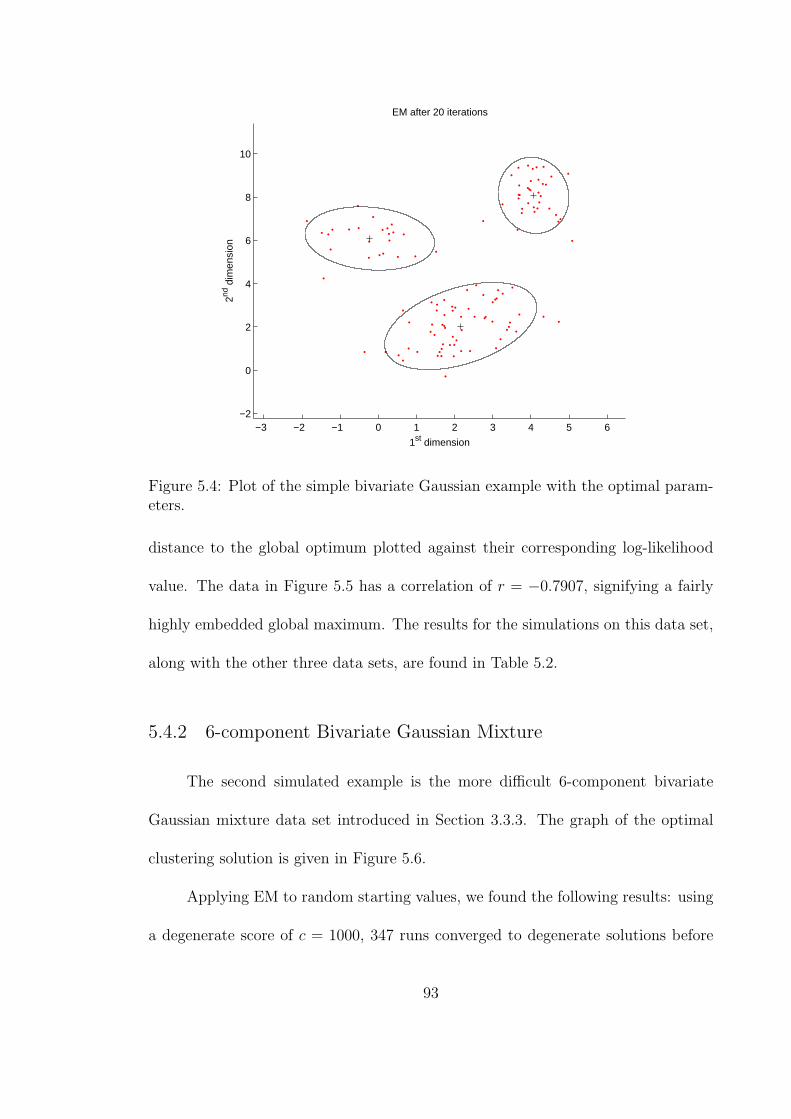
−3 −2 −1 0 1 2 3 4 5 6−2
0
2
4
6
8
10
1st dimension
2nd d
imen
sion
EM after 20 iterations
Figure 5.4: Plot of the simple bivariate Gaussian example with the optimal param-eters.
distance to the global optimum plotted against their corresponding log-likelihood
value. The data in Figure 5.5 has a correlation of r = −0.7907, signifying a fairly
highly embedded global maximum. The results for the simulations on this data set,
along with the other three data sets, are found in Table 5.2.
5.4.2 6-component Bivariate Gaussian Mixture
The second simulated example is the more difficult 6-component bivariate
Gaussian mixture data set introduced in Section 3.3.3. The graph of the optimal
clustering solution is given in Figure 5.6.
Applying EM to random starting values, we found the following results: using
a degenerate score of c = 1000, 347 runs converged to degenerate solutions before
93

0 1 2 3 4 5 6 7 8
−480
−470
−460
−450
−440
−430
−420
−410
Distance to Global Optimum
Log−
likel
ihoo
d
Local Solutions of 3−component Bivariate Gaussian
Figure 5.5: Plot of the local solutions of the simple bivariate Gaussian example,with their corresponding distance to the global optimum plotted against their cor-responding log-likelihood values.
the 500th non-degenerate solution. We estimate the relative size of the degenerate
region of attraction as pdeg = 347847
= 40.97%. 50 of the 500 non-degenerate EM runs
converged to the optimal value of -946.98. Thus we estimate the relative size of the
global optimum’s region of attraction to be A(y∗∗) = 50847
= 5.90% of the solution
space. Of the non-degenerate runs, we found N = 180 unique local optima. Figure
5.7 shows the plot of each of the non-degenerate local solutions found, with their
distance to the global optimum plotted against their corresponding log-likelihood
value. The data in Figure 5.7 has a correlation of r = −0.7872, signifying a fairly
highly embedded global maximum. The results for the simulations on this data set
are found in Table 5.2, at the end of this section.
94
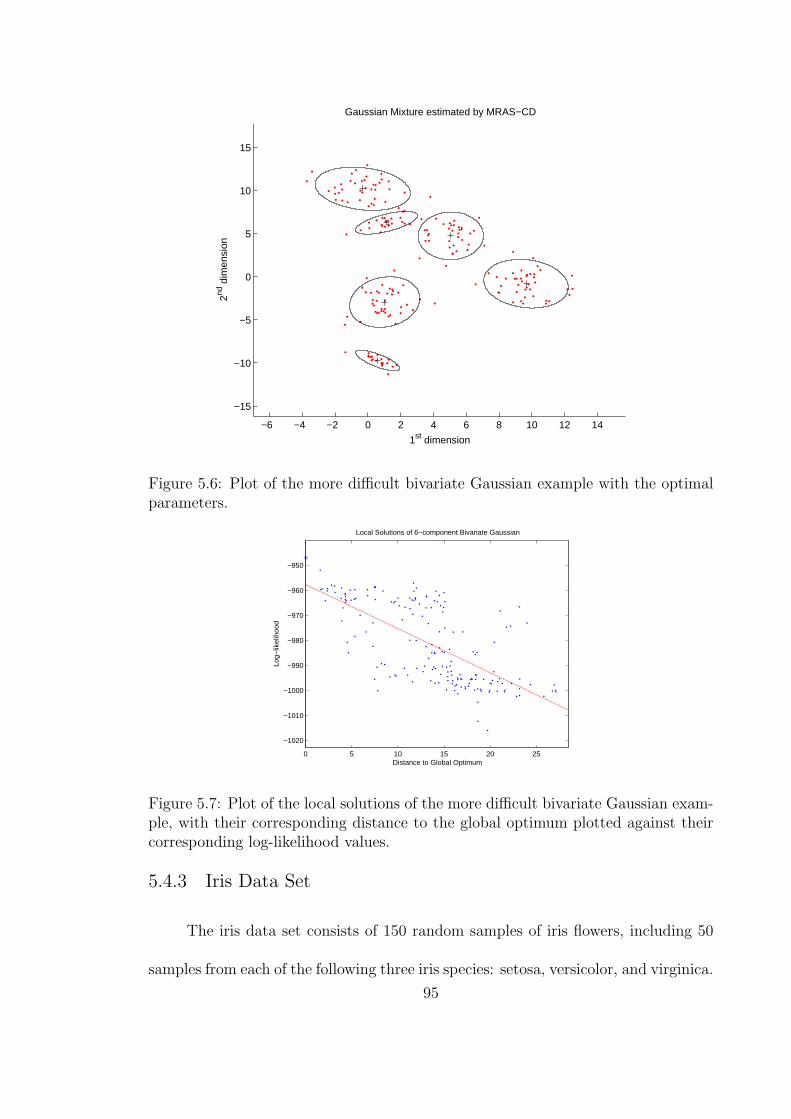
−6 −4 −2 0 2 4 6 8 10 12 14
−15
−10
−5
0
5
10
15
1st dimension
2nd d
imen
sion
Gaussian Mixture estimated by MRAS−CD
Figure 5.6: Plot of the more difficult bivariate Gaussian example with the optimalparameters.
0 5 10 15 20 25
−1020
−1010
−1000
−990
−980
−970
−960
−950
Distance to Global Optimum
Log−
likel
ihoo
d
Local Solutions of 6−component Bivariate Gaussian
Figure 5.7: Plot of the local solutions of the more difficult bivariate Gaussian exam-ple, with their corresponding distance to the global optimum plotted against theircorresponding log-likelihood values.
5.4.3 Iris Data Set
The iris data set consists of 150 random samples of iris flowers, including 50
samples from each of the following three iris species: setosa, versicolor, and virginica.
95

The data was collected by Anderson (1935). Each data sample consists of four
measurements: sepal length, sepal width, petal length, and petal width, all measured
in centimeters. The iris data set gained notoriety when Fisher (1936) developed a
linear discriminant model to classify the species from the data measurements. Figure
5.8 depicts the 1st and 2nd principal components of the data, along with the optimal
clustering solution, corresponding to a log-likelihood value of -180.19.
−4 −3 −2 −1 0 1 2 3 4 5
−1.5
−1
−0.5
0
0.5
1
1.5
1st Component
2nd
Com
pone
nt
Iris Data Set
Figure 5.8: Plot of the 1st and 2nd principal components of the iris data set, alongwith the corresponding optimal solution.
Applying EM to random starting values, we found the following results: using
a degenerate score of c = 10, 000, 67 runs converged to degenerate solutions before
the 500th non-degenerate solution. We estimate the relative size of the degenerate
region of attraction as pdeg = 67567
= 11.82%. 277 of the 500 non-degenerate EM
runs converged to the optimal value of -180.19. Thus we estimate the relative
96

size of the global optimum’s region of attraction to be A(y∗∗) = 277567
= 48.85% of
the solution space. Of the non-degenerate runs, we found N = 11 unique local
optima. Figure 5.9 shows the plot of each of the non-degenerate local solutions
found, with their distance to the global optimum plotted against their corresponding
log-likelihood value. The data in Figure 5.9 has a correlation of r = −0.7362,
signifying a moderately embedded global maximum. The results for the simulations
on this data set are found in Table 5.2, at the end of this section.
0 1 2 3 4 5 6
−320
−300
−280
−260
−240
−220
−200
−180
−160
−140
Distance to Global Optimum
Log−
likel
ihoo
d
Local Solutions of Iris Data Set
Figure 5.9: Plot of the local solutions of the iris data set, with their correspondingdistance to the global optimum plotted against their corresponding log-likelihoodvalues.
5.4.4 Control Chart Data
This data set consists of 600 control charts synthetically generated by the
process in Alcock and Manolopoulos (1999). There are six different classes of control
97

charts in the data: normal, cyclic, increasing trend, decreasing trend, upward shift,
and downward shift. Each chart consists of a 60-dimensional vector. The goal is to
cluster the charts into six groups, where each group represents one of the control
chart classes. Figure 5.10 depicts the 1st and 2nd principal components of the data,
along with the optimal clustering solution, corresponding to a log-likelihood value of
-92799. Note that since we know the true memberships of each data point, in order
to produce the global otpimum, we intiated each cluster component’s parameters
with that particular cluster’s maximum likelihood paramters, and then ran EM.
−150 −100 −50 0 50 100 150−60
−40
−20
0
20
40
60
80
100
1st Component
2nd
Com
pone
nt
Control Chart Data Set
Figure 5.10: Plot of the 1st and 2nd principal components of the control chart dataset, along with the corresponding optimal solution.
Applying EM to random starting values, we found the following results: using
a degenerate score of c = 10100, 521 runs converged to degenerate solutions before
the 500th non-degenerate solution. We estimate the relative size of the degenerate
98

region of attraction as pdeg = 5211021≈ 51.03%. Of the 500 non-degenerate runs, we
found N = 439 unique local optima. Perhaps due to the high dimensionality of
the data, we found many local optima (a total of 429) with a better log-likelihood
value than what we initially thought was the global optimum. The best solution
found has a log-likelihood value of -72803. Because of the extremely high number
of local optima, it is unclear whether this solution is the true global optimum of the
data. Only a single run of the 500 non-degenerate solutions converged to the best
solution found, and so we estimate the relative size of the global optimum’s region of
attraction to be A(y∗∗) = 11021≈ 0.10% of the solution space. Figure 5.11 shows the
plot of each of the non-degenerate local solutions found, with their distance to the
global optimum plotted against their corresponding log-likelihood value. The data
in Figure 5.11 has a correlation of r = −0.8317, signifying a fairly highly embedded
global maximum. The results for the simulations on this data set are found in Table
5.2, in the following section.
Figure 5.12 shows the plot of the 1st and 2nd principal components of many
clusterings that have better log-likelihood values than the solution found in Figure
5.10. This is an interesting find, because if we did not know the true memberships
of the data points, these results by clustering using Gaussian mixtures would lead
us to believe that the true global optimum is a relatively poor solution, simply by
comparing the log-likelihood values. In fact, two of the clusterings (the two on the
right of Figure 5.12) lead us to believe that the data may only have 5 clusters, as
2 of the clusters sit on top of one another. This example shows us that there are
instances where Gaussian mixture clusterings may have better likelihood values, yet
99

0 50 100 150 200 250 300 350 400−9.5
−9
−8.5
−8
−7.5
x 104
Distance to Global Optimum
Log−
likel
ihoo
d
Local Solutions of Control Chart Data Set
Figure 5.11: Plot of the local solutions of the control chart data set, with theircorresponding distance to the global optimum plotted against their correspondinglog-likelihood values.
in actuality do a poorer job of correctly classifying the true memberships of the
data. As evidenced by this example, this occurrence may be due to the complexity
brought on by the high dimensionality of the data.
5.4.5 Summary of Results
Table 5.2 summarizes the results of the four Gaussian mixture model examples.
We report the number of clusters, dimensionality, relative size of the region of at-
traction of the global optimum, number of unique local optima found, embeddedness
correlation, and the relative size of the degenerate region of attraction. Obviously
the control chart data set is the most difficult to optimize, as evidenced by its low
100
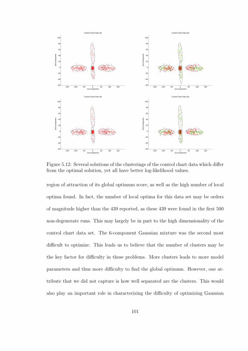
−150 −100 −50 0 50 100 150−60
−40
−20
0
20
40
60
80
100
1st Component
2nd
Com
pone
nt
Control Chart Data Set
−150 −100 −50 0 50 100 150−60
−40
−20
0
20
40
60
80
100
1st Component
2nd
Com
pone
nt
Control Chart Data Set
−150 −100 −50 0 50 100 150−60
−40
−20
0
20
40
60
80
100
1st Component
2nd
Com
pone
nt
Control Chart Data Set
−150 −100 −50 0 50 100 150−60
−40
−20
0
20
40
60
80
100
1st Component
2nd
Com
pone
nt
Control Chart Data Set
Figure 5.12: Several solutions of the clusterings of the control chart data which differfrom the optimal solution, yet all have better log-likelihood values.
region of attraction of its global optimum score, as well as the high number of local
optima found. In fact, the number of local optima for this data set may be orders
of magnitude higher than the 439 reported, as these 439 were found in the first 500
non-degenerate runs. This may largely be in part to the high dimensionality of the
control chart data set. The 6-component Gaussian mixture was the second most
difficult to optimize. This leads us to believe that the number of clusters may be
the key factor for difficulty in these problems. More clusters leads to more model
parameters and thus more difficulty to find the global optimum. However, one at-
tribute that we did not capture is how well separated are the clusters. This would
also play an important role in characterizing the difficulty of optimizing Gaussian
101

mixture models.
Table 5.2: Simulation results on four Gaussian mixtures.
Data Set g dimensionality A(y∗∗) N r pdeg
3-component Gaussian 3 2 77.24% 14 -.7907 13.79%6-component Gaussian 6 2 5.90% 180 -.7872 40.97%
Iris 3 4 48.85% 11 -.7362 11.82%Control Chart 6 60 0.10% 439 -.8317 51.03%
We also notice that the embeddedness correlation coefficients were all fairly
similar. This may signify that Gaussian mixture model problems are all roughly
equivalent in terms of embeddedness, thus relegating the embeddedness criterion to
be very minor in terms of its effect on optimization difficulty. Another interesting
deduction from the table is that the problems with higher number of clusters also
have a larger proportion of degenerate solutions. This could be attributed to the
idea that the more clusters we optimize, the higher probability that at least one of
them will get stuck in a degenerate solution centered on a single point.
5.5 Discussion
Many factors play a role in the difficulty of a given optimization problem.
Some of these factors, such as the region of attraction of ε-optimal solutions, only
have significance in certain problem settings. It would be nice to be able to gauge
the difficulty of a given optimization problem with a single metric. However, as
mentioned, this unified metric would likely be different for different classes of op-
timization problems, e.g., Gaussian mixture models being one. Also, in terms of
102

mixture models, a metric for how well-separated are the clusters in a mixture would
definitely help the characterization of the optimization difficulty. Furthermore, an-
alyzing how the dimensionality, number of clusters, and number of data points of a
data set affect these landscape measures would potentially lead to new and useful
insight on the landscape of Gaussian mixtures.
Another extension to the work in this chapter could be to combine the re-
sults found for a given optimization problem with extreme value theory to estimate
the true global optimum. Golden and Alt (1979) developed procedures for deter-
mining interval estimates for intractable global optima of NP-hard combinatorial
optimization problems, and so an analogous procedure could be applied to mixture
models.
103

Chapter 6
Conclusions
Perhaps the biggest current limitation of the CE and MRAS mixture model
algorithms is the computational time to convergence. Because the proposed algo-
rithms require the generation of multiple candidate solutions in each iteration, they
are inherently more computationally-intensive algorithms than EM. This is similar
in nature to the Monte Carlo EM algorithm (Booth and Hobert, 1999; Levine and
Casella, 2001; Levine and Fan, 2003; Jank, 2004; Caffo et al., 2003), which spends
most of its computational effort on simulating from a suitable distribution and is
thus much slower than its deterministic counterpart. That being said, our current
implementation of the CE and MRAS mixture model algorithms are not optimized
for speed, and continuous advances in computing power and processor speed will
make the computational disadvantages less practically important. At the end of the
day, the decision that researchers faces is whether one wants fast but possibly highly
inaccurate answers, or alternatively whether waiting a little longer is worth obtain-
ing better solutions. The algorithms proposed in Chapter 3 are systematic ways for
finding those solutions. However, part of my future plans include optimizing these
algorithms for better run times. Additional future work would include generalizing
the objective function in order to find the best clustering across all values of g.
Also, we would like to characterize how the run-time complexity of the proposed
104

algorithms changes with respect to problem size.
In Chapter 4 we presented a proof of global convergence of the MRAS-CD
algorithm to the optimal solution for Gaussian mixtures. One possible path of future
work could include extending the proof to finite mixture models of other probability
distributions, in addition to Gaussian. In addition, proving the convergence of the
other three algorithms presented in Chapter 3 is an open problem.
Chapter 5 discussed many factors that play a role in the difficulty of a given
optimization problem. Some of these factors, such as the region of attraction of ε-
optimal solutions, only have significance in certain problem settings. It would useful
to combine all of the metrics discussed into a single metric. However, this unified
metric would likely be different for different classes of optimization problems. Also,
in terms of mixture models, a metric for how well-separated are the clusters in a
mixture would characterize optimization difficulty. Furthermore, analyzing how the
dimensionality, number of clusters, and number of data points of a data set affect
these landscape measures would potentially lead to new and useful insights on the
landscape of Gaussian mixtures.
105

Bibliography
Alcock, R. J. and Manolopoulos, Y. (1999). Time-Series Similarity Queries Em-ploying a Feature-Based Approach. In 7th Hellenic Conference on Informatics,Ioannina, Greece.
Anderson, E. (1935). The Irises of the Gaspe Peninsula. Bulletin of the AmericanIris Society, 59:2–5.
Biernacki, C., Celeux, G., and Govaert, G. (2003). Choosing Starting Values forthe EM Algorithm for Getting the Highest Likelihood in Multivariate GaussianMixture Models. Computational Statistics & Data Analysis, 41(3-4):561–575.
Booth, J. G. and Hobert, J. P. (1999). Maximizing Generalized Linear Mixed ModelLikelihoods with an Automated Monte Carlo EM Algorithm. Journal of the RoyalStatistical Society B, 61:265–285.
Botev, Z. and Kroese, D. P. (2004). Global Likelihood Optimization via the Cross-Entropy Method with an Application to Mixture Models. In Proceedings of the2004 Winter Simulation Conference.
Caffo, B. S., Jank, W. S., and Jones, G. L. (2003). Ascent-Based Monte Carlo EM.Journal of the Royal Statistical Society B, 67:235–252.
Cao, G. and West, M. (1996). Practical Bayesian Inference Using Mixtures of Mix-tures. Biometrics, 52:1334–1341.
Celeux, G. and Govaert, G. (1992). A Classification EM Algorithm for Cluster-ing and Two Stochastic Versions. Computational Statistics & Data Analysis,14(3):315–332.
De Boer, P., Kroese, D. P., Mannor, S., and Rubinstein, R. Y. (2005). A Tutorialon the Cross-Entropy Method. Annals of Operations Research, 134:19–67.
De Jong, K. A. (1975). An Analysis of the Behaviour of a Class of Genetic AdaptiveSystem. PhD thesis, University of Michigan, Ann Arbor, MI.
Dempster, A. P., Laird, N. M., and Rubin, D. B. (1977). Maximum Likelihood fromIncomplete Data via the EM Algorithm. Journal of the Royal Statistical SocietyB, 39:1–22.
Diebolt, J. and Robert, C. P. (1990). Bayesian Estimation of Finite Mixture Dis-tributions: Part II, Sampling Implementation. Technical Report III, Laboratoirede Statistique Theorique et Appliquee, Universite Paris VI.
Fisher, R. A. (1936). The Use of Multiple Measurements in Taxonomic Problems.Annals of Eugenics, 7:179–188.
106

Fraley, C. and Raftery, A. E. (1998). How Many Clusters? Which ClusteringMethod? Answers via Model-Based Cluster Analysis. The Computer Journal,41:578–588.
Golden, B. L. and Alt, F. B. (1979). Interval Estimation of a Global Optimum forLarge Combinatorial Problems. Naval Research Logistics Quarterly, 26:69–77.
Goldstein, A. A. and Price, I. F. (1971). On Descent from Local Minima. Mathe-matics of Computation, 25(115):569–574.
Heath, J., Fu, M., and Jank, W. (2007a). Global Convergence of Model ReferenceAdaptive Search for Gaussian Mixtures. Working Paper, Smith School of Business,University of Maryland.
Heath, J., Fu, M., and Jank, W. (2007b). New Global Optimization Algorithms forModel-Based Clustering. Working Paper, Smith School of Business, University ofMaryland.
Horn, R. A. and Johnson, C. R. (1990). Matrix Analysis. Cambridge Univ. Press,New York.
Hu, J., Fu, M. C., and Marcus, S. I. (2007). A Model Reference Adaptive SearchAlgorithm for Global Optimization. Operations Research, 55(3). In press.
Jamshidian, M. and Jennrich, R. I. (1993). Conjugate Gradient Acceleration of theEM Algorithm. Journal of the American Statistical Association, 88:221–228.
Jamshidian, M. and Jennrich, R. I. (1997). Acceleration of the EM Algorithm byusing Quasi-Newton Methods. Journal of the Royal Statistical Society B, 59:569–587.
Jank, W. (2004). Quasi-Monte Carlo Sampling to Improve the Efficiency of MonteCarlo EM. Computational Statistics & Data Analysis, 48:685–701.
Jank, W. (2006a). Ascent EM for Fast and Global Model-Based Clustering: AnApplication to Curve-Clustering of Online Auctions. Computational Statistics &Data Analysis, 51(2):747–761.
Jank, W. (2006b). The EM Algorithm, Its Stochastic Implementation and GlobalOptimization: Some Challenges and Opportunities for OR. In Alt, F., Fu, M.,and Golden, B., editors, Perspectives in Operations Research: Papers in Honorof Saul Gass’ 80th Birthday, pages 367–392. Springer, New York.
Johnson, C. R. (1970). Positive Definite Matrices. The American MathematicalMonthly, 77(3):259–264.
Jones, T. and Forrest, S. (1995). Fitness Distance Correlation as a Measure ofProblem Difficulty for Genetic Algorithms. In Proceedings of the 6th InternationalConference on Genetic Algorithms, pages 184–192.
107

Kroese, D. P., Porotsky, S., and Rubinstein, R. Y. (2006). The Cross-EntropyMethod for Continuous Multi-Extremal Optimization. Methodology and Comput-ing in Applied Probability, 8:383–407.
Kroese, D. P., Rubinstein, R. Y., and Taimre, T. (2007). Application of the Cross-Entropy Method to Clustering and Vector Quantization. Journal of Global Opti-mization, 37(1):137–157.
Lagarias, J. C., Reeds, J. A., Wright, M. H., and Wright, P. E. (1998). ConvergenceProperties of the Nelder-Mead Simplex Method in Low Dimensions. SIAM Journalof Optimization, 9(1):112–147.
Levine, R. and Casella, G. (2001). Implementations of the Monte Carlo EM Algo-rithm. Journal of Computational and Graphical Statistics, 10:422–439.
Levine, R. and Fan, J. (2003). An Automated (Markov Chain) Monte Carlo EMAlgorithm. Journal of Statistical Computation and Simulation, 74:349–359.
Liu, C. and Rubin, D. B. (1994). The ECME algorithm: A Simple Extension of EMand ECM with Faster Monotone Convergence. Biometrika, 81:633–648.
Louis, T. A. (1982). Finding the Observed Information Matrix when Using the EMAlgorithm. Journal of the Royal Statistical Society B, 44:226–233.
Mangiameli, P., Chen, S., and West, D. (1996). A Comparison of SOM NeuralNetwork and Hierarchical Clustering Methods. European Journal of OperationalResearch, 93:402–417.
McLachlan, G. J. and Peel, D. (2000). Finite Mixture Models. Wiley, New York.
Meng, X. L. (1994). On the Rate of Convergence of the ECM Algorithm. TheAnnals of Statistics, 22:326–339.
Meng, X. L. and Rubin, D. B. (1993). Maximum Likelihood Estimation via theECM Algorithm: A General Framework. Biometrika, 80:267–278.
Milligan, G. W. (1981). A Review of Monte Carlo Tests of Cluster Analysis. Mul-tivariate Behavioral Research, 16:379–407.
Pinheiro, J. C. and Bates, D. M. (1996). Unconstrained Parameterizations forVariance-Covariance Matrices. Statistics and Computing, 6:289–296.
Reddy, C., Chiang, H., and Rajarathnam, B. (2006). Stability Region basedExpectation Maximization for Model-Based Clustering. In Proceedings of theIEEE/ACM International Conference on Data Mining (ICDM).
Rubinstein, R. Y. (1997). Optimization of Computer Simulation Models with RareEvents. European Journal of Operations Research, 99:89–112.
108

Rubinstein, R. Y. (1999). The Simulated Entropy Method for Combinatorial andContinuous Optimization. Methodology and Computing in Applied Probability,2:127–190.
Rubinstein, R. Y. and Kroese, D. P. (2004). The Cross-Entropy Method: A UnifiedApproach to Combinatorial Optimization, Monte-Carlo Simulation and MachineLearning. Springer-Verlag, New York.
Thisted, R. A. (1988). Elements of Statistical Computing. Chapman & Hall, London.
Torn, A., Ali, M. M., and Viitanen, S. (1999). Stochastic Global Optimiza-tion: Problem Classes and Solution Techniques. Journal of Global Optimization,14:437–447.
Tu, Y., Ball, M., and Jank, W. (2006). Estimating Flight Departure Delay Distri-butions - A Statistical Approach with Long-Term Trend and Short-Term Pattern.Forthcoming in the Journal of the American Statistical Association.
Ueda, N. and Nakano, R. (1998). Deterministic Annealing EM Algorithm. NeuralNetworks, 11(2):271–282.
Ward, Jr., J. H. (1963). Hierarchical Grouping to Optimize an Objective Function.Journal of the American Statistical Association, 58:236–244.
Wei, G. C. and Tanner, M. A. (1990). A Monte Carlo Implementation of the EMAlgorithm and the Poor Man’s Data Augmentation Algorithms. Journal of theAmerican Statistical Association, 85:699–704.
Wright, S. (1932). The Roles of Mutation, Inbreeding, Crossbreeding, and Selectionin Evolution. In Proceedings of the Sixth International Congress on Genetics,pages 355–366.
Wu, C. F. J. (1983). On the Convergence Properties of the EM Algorithm. TheAnnals of Statistics, 11(1):95–103.
109