330

NOAANational Marine Fisheries Service

Fishery Bulletin First U.S. Commissioner of Fisheries and founder

of Fishery Bulletin established 1881

Predicting potential fishing zones for Pacific saury (Cololabis saira) with maximum entropy models and remotely sensed data

Achmad F. Syah (contact author)1,2

Sei-Ichi Saitoh1,3

Irene D. Alabia3

Toru Hirawake1

Email address for contact author: fachrudinsyah@gmail.com

1 Laboratory of Marine Environment and Resource Sensing Faculty of Fisheries Sciences Hokkaido University 3-1-1 Minato-cho Hakodate 041-8611, Japan2 Department of Marine Science University of Trunojoyo Madura Jalan Raya Telang P.O. Box 2 Kamal Bangkalan-Madura, Indonesia3 Arctic Research Center Hokkaido University N21-W11 Kita-ku Sapporo 001-002, Japan

Manuscript submitted 20 July 2015.Manuscript accepted 12 May 2016.Fish. Bull.:330–342 (2016).Online publication date: 2 June 2016.doi: 10.7755/FB.114.3.6

The views and opinions expressed or implied in this article are those of the author (or authors) and do not necessarily reflect the position of the National Marine Fisheries Service, NOAA.

Abstract—Fishing locations for Pa-cific saury (Cololabis saira) obtained from images of the Operational Linescan System (OLS) of the U.S. Defense Meteorological Satellite Program, together with maximum entropy models and satellite-based oceanographic data of chlorophyll-a concentration (chl-a), sea-surface temperature (SST), eddy kinetic en-ergy (EKE), and sea-surface height anomaly (SSHA), were used to evalu-ate the effects of oceanographic con-ditions on the formation of potential fishing zones (PFZ) for Pacific saury and to explore the spatial variabil-ity of these features in the western North Pacific. Actual fishing regions were identified as the bright areas created by a 2-level slicing method for OLS images collected August–De-cember during 2005–2013. The re-sults from a Maxent model revealed its potential for predicting the spa-tial distribution of Pacific saury and highlight the use of multispectral satellite images for describing PFZs. In all monthly models, the spatial PFZ patterns were explained pre-dominantly by SST (14–16°C) and indicated that SST is the most influ-ential factor in the geographic distri-bution of Pacific saury. Also related to PFZ formation were EKE and SSHA, possibly through their effects on the feeding grounds conditions. Concentration of chl-a had the least effect among other environmental factors in defining PFZs, especially during the end of the fishing season.

The Pacific saury (Cololabis saira) is widely distributed in the west-ern North Pacific from subarctic to subtropical waters and is one of the commercially important pelagic spe-cies in Japan, Russia, Korea, and Taiwan. The total landings of this species in these countries increased from 171,692 metric tons (t) in 1998 to 449,738 t in 2011. Over the last half century, annual catches of Pacif-ic saury in Japan, for example, have averaged around 257,800 t (Tian et al., 2003) and have fluctuated greatly from 52,207 t in 1969 to 207,770 t in 2011 (Fisheries Agency and Fisheries Research Agency of Japan, 2012).

The number, size, and location of fishing grounds for Pacific saury are largely affected by oceanographic conditions (Yasuda and Watanabe, 1994; Kosaka, 2000; Tian et al., 2002), and the significant effect of

environmental factors on abundance of Pacific saury was evident in the unexpected drop in both the catch and catch per unit of effort in 1998, following a period of high abundance (Tian et al., 2003). The distribution and migratory patterns of Pacific saury have been associated with chlorophyll-a (chl-a) concentration and sea-surface temperature (SST) (Watanabe et al., 2006; Mukai et al., 2007; Tseng et al., 2013). More-over, sea-surface height indicates water mass movements and, by ex-tension, the flow of heat and nutri-ents, which will subsequently influ-ence productivity (Ayers and Lozier, 2010). Sea-surface height can also be used to infer physical oceanographic features, such as eddies, fronts, and convergences (Polovina and Howell, 2005). Therefore, understanding the relationship between oceanographic

Syah et al.: Predicting potential fishing zones for Cololabis saira 331

factors and the migration and distribution of species is essential for fisheries management.

Most studies of Pacific saury have concentrated on distribution and migration and have used in situ or logbook data (Huang et al., 2007; Tseng et al., 2013), and models have been developed to investigate growth and abundance (Tian et al., 2004; Ito et al., 2004, 2007; Mukaietal., 2007). In contrast, Watanabe et al. (2006) proposed a spatial and temporal migration model for stock size that was dependent on SST. However, inte-grated high-resolution nighttime satellite images, such as those available in the time-series data from the Op-erational Linescan System (OLS) of the Defense Me-teorological Satellite Program, U.S. Department of De-fense, together with habitat and environmental model-ing, have not been used to predict the potential fishing zones for Pacific saury.

In Japan, fishing vessels operate at night and use stick-held dip nets, locally known as bouke ami, which are equipped with lights to attract fishes (Fukushima, 1979). These fishing vessels, equipped with lights, as are vessels that fish for Pacific saury, can be identified by the OLS sensor, which also enables the detection of moonlight-illuminated clouds and lights from cit-ies, towns, industrial sites, gas flares, and ephemeral events, such as fires and lightning-illuminated clouds (Elvidge et al., 1997). In addition, OLS nighttime im-ages can be used to estimate fishing vessel numbers and fishing areas for squid (Kiyofuji and Saitoh, 2004; Kiyofuji et al., 2004). The relationship between the number of lit pixels in OLS nighttime images and the number of fishing vessels also has been analyzed for the fishery of Illex argentinus (Waluda et al., 2002). The brightly lit areas seen in nighttime images of the western North Pacific are the result of vessels fishing for Pacific saury or squid (Semedi et al., 2002; Saitoh et al., 2010; Mugo et al., 2014).

Predictive habitat modeling has become an increas-ingly useful tool for marine ecologists and conservation scientists in order to estimate the patterns of species distribution and to subsequently develop conservation strategies (Johnson and Gillingham, 2005; Tsoar et al., 2007; Ready et al., 2010). The maximum entropy method (Phillips et al., 2006) involves one of the most widely used machine-learning algorithms for inferring species distributions. In recent studies, the method of maximum entropy has been applied to both terrestrial (Peterson et al., 2007) and marine ecosystems (Ready et al., 2010; Edrén et al., 2010; Alabia et al., 2015). In this study, we used a maximum entropy approach with multi sensor satellite datasets and OLS-derived spe-cies occurrences to create an accurate prediction model and investigate the potential fishing zones for Pacific saury in the western North Pacific. The objectives of this study were to evaluate the effects of oceanographic factors on the formation of potential fishing zones for Pacific saury and to examine the variability in spatial patterns of potential fishing zones in relation to the prevailing oceanographic conditions in the western North Pacific.

Materials and methods

Study area

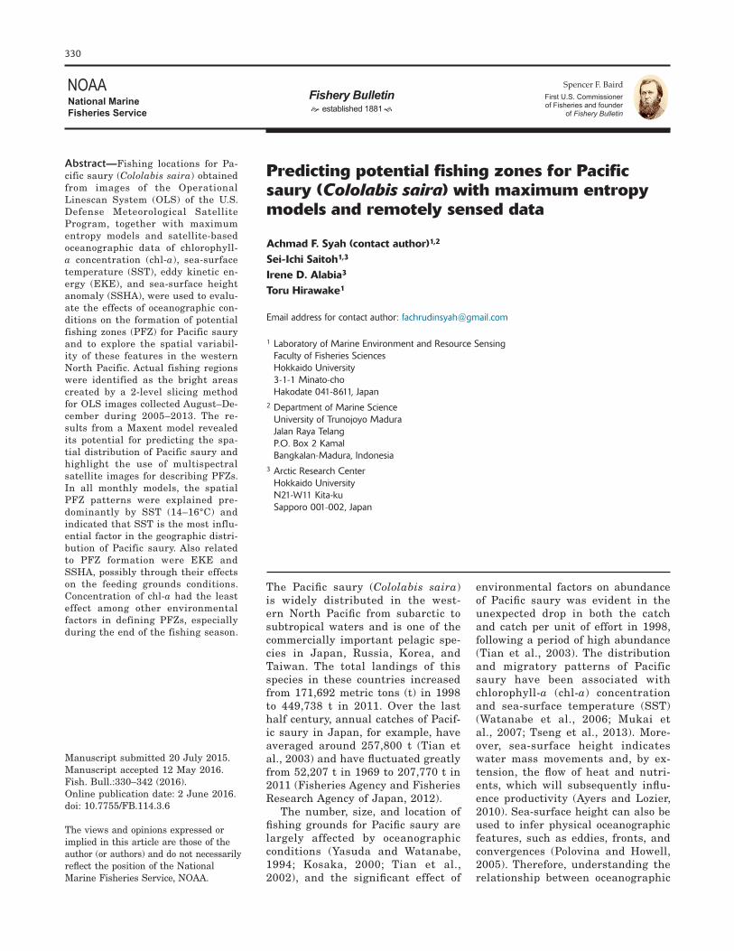
This study was conducted in the western North Pacific, extending from 140° to 155°E and from 34° to 46°N (Fig. 1). In this study area, located between the sub-arctic and subtropical domains of the North Pacific, the confluence of the warm Kuroshio Current and the cold Oyashio Current forms the Kuroshio–Oyashio transition zone (Roden, 1991), also called the subarc-tic–subtropical transition zone. The Kuroshio Current is characterized by warm, low-density, nutrient-poor, and high-salinity surface waters (Yatsu et al., 2013), whereas the Oyashio Current is characterized by low-salinity, low-temperature, and nutrient-rich waters (Sakurai, 2007). The Kuroshio–Oyashio transition zone is characterized by the mixing of various water masses and complex physical oceanographic structures (Roden, 1991). Moreover, 3 major oceanic fronts exist in this region: the Polar Front, Subarctic Front, and Kuroshio Extension Front (Science Council of Japan1). The characteristic patterns of these oceanic fronts also have been well documented in earlier studies (Kitano, 1972; Roden et al., 1982; Belkin and Mikhailichenko, 1986; Miyake, 1989; Belkin et al., 1992, 2002; Yoshida, 1993; Onishi, 2001; Murase et al., 2014; Shotwell et al., 2014).

Satellite nighttime images

Daily cloud-free OLS nighttime images were download-ed from the Satellite Image Database System of the Agriculture, Forestry and Fisheries Research Informa-tion Center of the Japan Ministry of Agriculture, For-estry and Fisheries [the system is no longer operating]. The images were then used to determine the location of the vessels that fish for Pacific saury in the western North Pacific. A TeraScan2 system, vers. 4.0 (Seaspace Corp., Poway, CA) was used to analyze the images and to process the nighttime lights into digital numbers (DNs), in a range of 0–63, that represent the visible pixels in relative values. We selected 1264 single pass images collected from August through December dur-ing 2005–2013 (9 years) by 6 Defense Meteorological Satellite Program satellites (F13, F14, F15, F16, F17, and F18) (Table 1). The period from August through December was chosen for analysis because it corre-sponds with the fishing season of Pacific saury. To con-struct the habitat suitability model, the daily images were reprocessed with a 1-km resolution and then com-piled in a monthly database. The location of the vessels was assumed to represent the location of Pacific saury.

1 Science Council of Japan. 1960. The results of the Japa-nese oceanographic project for the International Geophysical Year 1957/8, 145 p. National Committee for the Interna-tional Geophysical Year, Science Council of Japan, Tokyo.

2 Mention of trades names or commercial companies is for identification purposes only and does not imply endorsement by the National Marine Fisheries Service, NOAA.

332 Fishery Bulletin 114(3)

Detection of fishing vessel

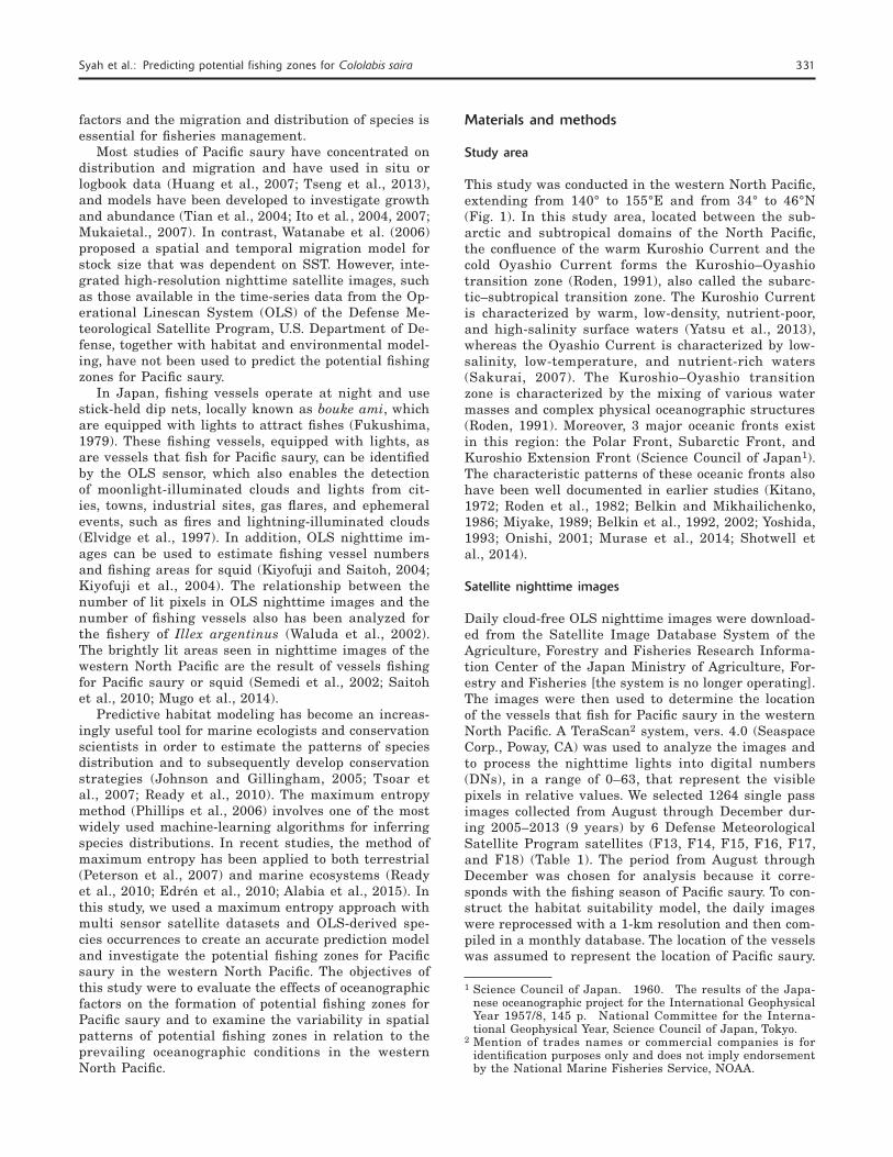
We examined the histograms of DNs in our analyses of OLS images for each month in order to identify the fishing areas. Several peaks in DNs were recorded over the examined 5-month periods (Fig. 2). To extract the areas with fishing-vessel lights, DN thresholds for identifying Pacific saury fishing vessels were calculated for each month because of the monthly differences in DN frequency distribution. A 2-level slicing method was used to extract the bright areas thought to be caused by the fishing fleet. This method is used to find a statistical optimum threshold from the DN frequency distribution (Takagi and Shimoda, 1991).

The thresholds, k, were determined through the use of the following method proposed by Kiyofuji and Saitoh (2004), and the variance, σ2(k), was calculated with the equations proposed by Takagi and Shimoda (1991):

σ2(k)=ωo(µo−µT)2 + ω1 (µ1−µT)2, (1)

where ni = the number of pixels at i levels; N = the total number of pixels; Pi = ni/N; ω0 = Pii=1

k∑ and ω1 = Pii=k+1l∑ ;

µ0 = iPii=1k∑ /ωo and µ1 = iPii=k+1

l∑ /ω1; µT = iPii=1

l∑ .

With these methods, 5 thresholds were identified (Table 2). Class 1, 2, 3, and 4 thresholds indicate ocean water or cloud coverage, and the class 5 threshold indicates bright areas resulting from fishing vessel lights. There-fore, class 5 threshold values were applied to extract the bright areas that represented fishing vessel lights.

Lights from vessels that fish for Pacific saury and those that fish for squid are contained in OLS images. These lights are difficult to distinguish from each other; therefore, it is necessary to generate OLS images with less contamination from the lights of vessels fishing for

Figure 1Map of the study area in the western North Pacific with the hydro-graphic and topographic features of the ocean basin. The line with dashes and dots represents the boundary of the EEZ of Japan. The lines with dashes correspond to the 3 major oceanic fronts—the Po-lar Front (PF), Subartic Front (SAF), and Kuroshio Extension Front (KEF). The subarctic–subtropical transition zone is also shown. Re-drawn after Murase et al. (2014).

140°E 142°E 144°E 146°E 148°E 150°E 152°E 154°E46°N

44°N

42°N

40°N

38°N

36°N

34°N

–8000 –6000 –4000 –2000 0

Depth (m)

Syah et al.: Predicting potential fishing zones for Cololabis saira 333

squid. In this study, we used SST to distinguish between the lights of the vessels that fish for Pacific saury and those of other fishing vessels because Pacific saury prefers colder areas for their migration routes (Saitoh et al., 1986) and this approach was used earlier by Mugo et al. (2014).

Because Pacific saury are dis-tributed below the upper SST limit (Table 3), we split the nighttime light images into 2 categories. All lights that occurred above the upper SST limit were categorized as lights re-lated to squid fishing, and all lights that occurred below this limit were assumed to be from vessels fishing for Pacific saury. Consequently, only the locations of lights that indicated fishing for Pacific saury were used for our habitat modeling procedures.

Environmental data

We used satellite-derived data—chl-a, SST, eddy kinetic energy (EKE), and sea-surface height anomaly (SSHA)—from 2005 through 2013 as environmental factors in the maxi-mum entropy models. Daily chl-a and SST values were derived from satellite images from the Moder-ate Resolution Imaging Spectroradi-ometer (MODIS)-Aqua mission and were downloaded from NASA God-dard Space Flight Center [website]. These data were processed with the SeaDAS package, vers. 6.4 (NASA Goddard Space Flight Center, Green-belt, MD) and reprocessed to create maps with a 1-km resolution.

Daily SSHA and geostrophic ve-locities (u, v) from the Topex/Posei-don and ERS-1/2 altimeters were

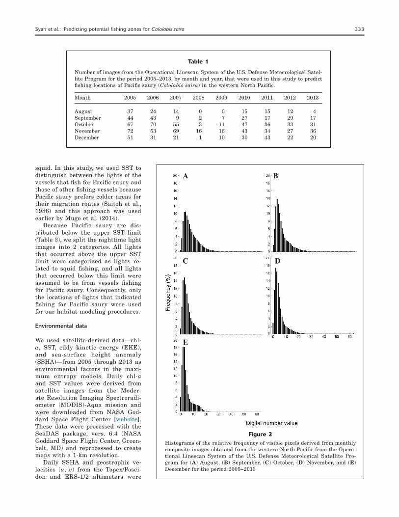
Table 1

Number of images from the Operational Linescan System of the U.S. Defense Meteorological Satel-lite Program for the period 2005–2013, by month and year, that were used in this study to predict fishing locations of Pacific saury (Cololabis saira) in the western North Pacific.

Month 2005 2006 2007 2008 2009 2010 2011 2012 2013

August 37 24 14 0 0 15 15 12 4September 44 43 9 2 7 27 17 29 17October 67 70 55 3 11 47 36 33 31November 72 53 69 16 16 43 34 27 36December 51 31 21 1 10 30 43 22 20

Figure 2Histograms of the relative frequency of visible pixels derived from monthly composite images obtained from the western North Pacific from the Opera-tional Linescan System of the U.S. Defense Meteorological Satellite Pro-gram for (A) August, (B) September, (C) October, (D) November, and (E) December for the period 2005–2013

A B

C D

E

334 Fishery Bulletin 114(3)

produced and distributed by Archiving Validation and Interpretation of Satellite Oceanographic Data (AVISO; website) at a spatial resolution of 0.33°×0.33°. The sur-face geostrophic velocities were used to compute for EKE by using the following equation (Steele et al., 2010):

EKE = ½ (u’2 + v’2), (2)

where u’ and v’ = the zonal and meridional components of geostrophic currents, respectively.

With the grid function of the software package Ge-neric Mapping Tools, vers. GMT 4.5.7 (website),we were able to calculate the monthly averages for each environmental variable from daily data sets, resampled to 1-km resolution and converted to Esri ASCII grid format(Esri, Redlands, CA) or to comma-separated val-ues (CSV) format, as required by the software program Maxent (website).

Construction of a maximum entropy model

To develop a model with a maximum entropy approach, we used the software program Maxent, vers. 3.3.3k. Phillips et al. (2006) provided detailed information on the mode of operating this software. We constructed models using default values for regulation parameter (1), maximum iteration (500), and automatic feature class selection. We used a cross-validation procedure to evaluate the performance of the models. For back-ground points, we generated pseudo-absences (10:1 ratio of pseudo-absence to presence) following Barbet-Massin et al., (2012) on the basis of random spatial sampling within the study area (excluding points of presence of Pacific saury). We used the density.tools.RandomSample command line in Maxent to generate the random pseudo-absences. For each monthly model, the data were randomly split into 2 categories: one category for training data (70%) and one for test data (30%). The test points were then used to calculate the

Table 2

Thresholds for digital numbers (in pixels) for satellite images from the Operational Linescan System of the U.S. Defense Meteorological Satellite Program for the period 2005–2013. Thresholds were calculated from the histogram in Figure 2. Pixels within the class 5 range represent fishing vessel lights. Classes 1–4 represent reflected light from ocean water or light from cloud cover.

Month Class 1 Class 2 Class 3 Class 4 Class 5

August 10 17 23 30 40September 9 16 22 28 38October 8 14 19 27 38November 8 13 19 28 38December 7 12 18 27 38

Table 3

Mean monthly sea-surface temperature (SST) values (°C) and standard deviations (SD), used to distinguish the light of vessels fishing for Pacific saury (Cololabis saira) from the lights of fishing fleets fishing for other fish. All lights occurring below the upper SST limit were categorized as locations of vessels targeting Pa-cific saury.

Month Mean SD Upper SST limit

August 20.79 2.69 23.48 September 18.89 2.47 21.36 October 15.90 2.58 18.48 November 14.56 2.88 17.44 December 13.60 2.89 16.49

area under the curve (AUC) of the receiver operating characteristic (ROC) (Phillips et al., 2006).

Evaluation and validation of the model

We used the AUC metric of the ROC curve to evaluate model fit (Elith et al., 2006; Phillips et al., 2006). The relative contribution of individual environmental vari-ables within the maximum entropy model was exam-ined by using the heuristic estimates of variable impor-tance based on the increase in the model gain, which is associated with each environmental factor and its cor-responding model feature. Response curves generated for each factor were examined to derive the favorable environmental ranges for potential fishing zones.

Independent sets of monthly OLS data from 2011 through 2013 were used to validate the models. The base models were used to create habitat suitability indices (HSIs) that assimilated similar environmental layers for the corresponding period from 2011 through 2013. Spatial HSI maps were generated and over-lain with information on OLS data from the period 2011–2013.

Results

Spatiotemporal distribution of fishing locations, and envi-ronmental data

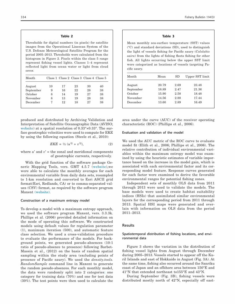
Figure 3 shows the variation in the distribution of fishing vessel lights from August through December during 2005–2013. Vessels started to appear off the Ku-ril Islands and east of Hokkaido in August (Fig. 3A). At the same time, fishing also occurred around the Sanriku coast of Japan and an offshore area between 150°E and 41°N that extended northeast to155°E and 43°N.

During September (Fig. 3B), fishing vessels were distributed mostly north of 42°N, especially off east-

Syah et al.: Predicting potential fishing zones for Cololabis saira 335

ern Hokkaido, whereas the number of vessels off the Sanriku coast decreased. In October (Fig. 3C), fishing vessels were widely distributed in Hokkaido and San-riku waters. The distribution of fishing vessels moved slightly to the south and approached the shores of southeastern Hokkaido and Sanriku (38–41°N). During this same month, the offshore fishing locations (148°E and 48°N) also increased and extended northeast to 154°E and 43°N.

During November (Fig. 3D), fishing vessels moved southward. The number of fishing vessels in eastern Hokkaido waters decreased, but the number of fishing vessels around the Sanriku coast increased (38–41°N) and moved northeast to 155°E and 43°N. A small num-ber of fishing vessels also appeared off the Joban coast. In December (Fig. 3E), fishing vessels appeared mostly along the Sanriku coast and were distributed in near-shore waters between 38°N and 40°N; however, a small number of fishing vessels still remained offshore and along the Joban coast.

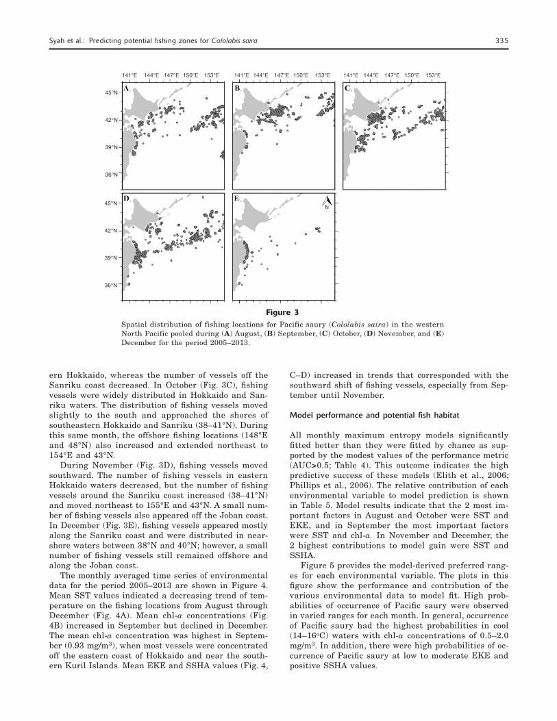
The monthly averaged time series of environmental data for the period 2005–2013 are shown in Figure 4. Mean SST values indicated a decreasing trend of tem-perature on the fishing locations from August through December (Fig. 4A). Mean chl-a concentrations (Fig. 4B) increased in September but declined in December. The mean chl-a concentration was highest in Septem-ber (0.93 mg/m3), when most vessels were concentrated off the eastern coast of Hokkaido and near the south-ern Kuril Islands. Mean EKE and SSHA values (Fig. 4,

C–D) increased in trends that corresponded with the southward shift of fishing vessels, especially from Sep-tember until November.

Model performance and potential fish habitat

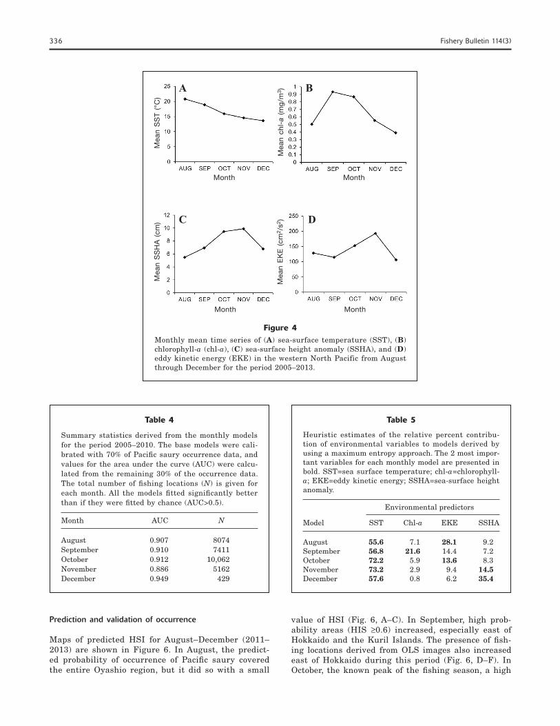
All monthly maximum entropy models significantly fitted better than they were fitted by chance as sup-ported by the modest values of the performance metric (AUC>0.5; Table 4). This outcome indicates the high predictive success of these models (Elith et al., 2006; Phillips et al., 2006). The relative contribution of each environmental variable to model prediction is shown in Table 5. Model results indicate that the 2 most im-portant factors in August and October were SST and EKE, and in September the most important factors were SST and chl-a. In November and December, the 2 highest contributions to model gain were SST and SSHA.

Figure 5 provides the model-derived preferred rang-es for each environmental variable. The plots in this figure show the performance and contribution of the various environmental data to model fit. High prob-abilities of occurrence of Pacific saury were observed in varied ranges for each month. In general, occurrence of Pacific saury had the highest probabilities in cool (14–16oC) waters with chl-a concentrations of 0.5–2.0 mg/m3. In addition, there were high probabilities of oc-currence of Pacific saury at low to moderate EKE and positive SSHA values.

Figure 3Spatial distribution of fishing locations for Pacific saury (Cololabis saira) in the western North Pacific pooled during (A) August, (B) September, (C) October, (D) November, and (E) December for the period 2005–2013.

141°E 144°E 147°E 150°E 153°E 141°E 144°E 147°E 150°E 153°E 141°E 144°E 147°E 150°E 153°E

45°N

42°N

39°N

36°N

45°N

42°N

39°N

36°N

336 Fishery Bulletin 114(3)

Table 5

Heuristic estimates of the relative percent contribu-tion of environmental variables to models derived by using a maximum entropy approach. The 2 most impor-tant variables for each monthly model are presented in bold. SST=sea surface temperature; chl-a=chlorophyll-a; EKE=eddy kinetic energy; SSHA=sea-surface height anomaly.

Environmental predictors

Model SST Chl-a EKE SSHA

August 55.6 7.1 28.1 9.2September 56.8 21.6 14.4 7.2October 72.2 5.9 13.6 8.3November 73.2 2.9 9.4 14.5December 57.6 0.8 6.2 35.4

Table 4

Summary statistics derived from the monthly models for the period 2005–2010. The base models were cali-brated with 70% of Pacific saury occurrence data, and values for the area under the curve (AUC) were calcu-lated from the remaining 30% of the occurrence data. The total number of fishing locations (N) is given for each month. All the models fitted significantly better than if they were fitted by chance (AUC>0.5).

Month AUC N

August 0.907 8074September 0.910 7411October 0.912 10,062November 0.886 5162December 0.949 429

Figure 4Monthly mean time series of (A) sea-surface temperature (SST), (B) chlorophyll-a (chl-a), (C) sea-surface height anomaly (SSHA), and (D) eddy kinetic energy (EKE) in the western North Pacific from August through December for the period 2005–2013.

A B

C D

Month Month

Month Month

Mea

n S

ST

(°C

)M

ean

SS

HA

(cm

)

Prediction and validation of occurrence

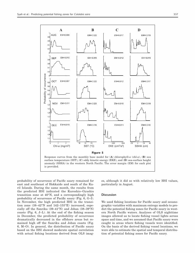
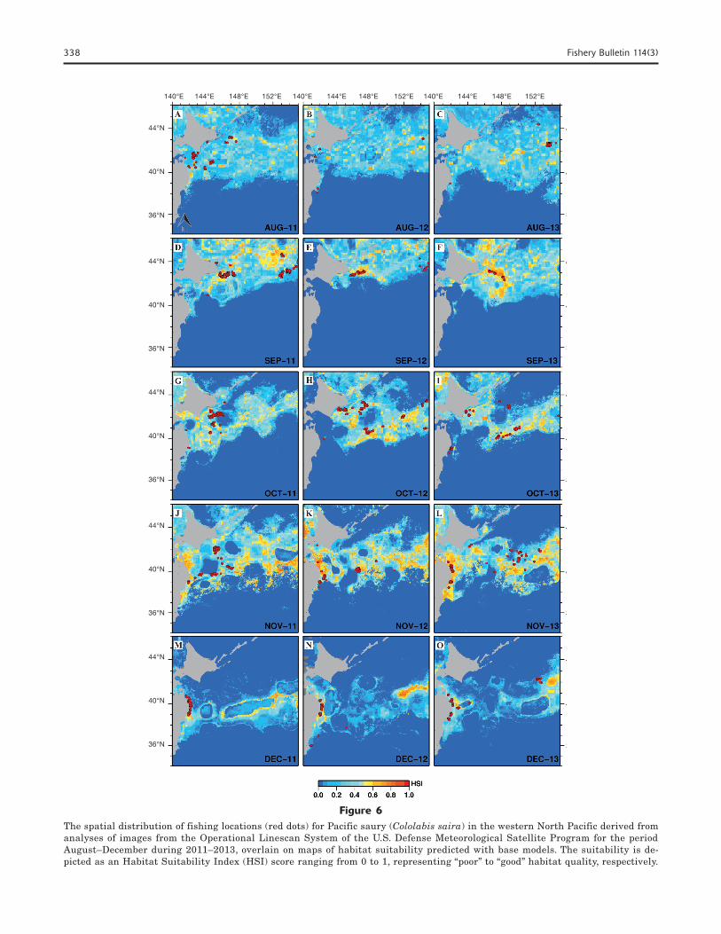
Maps of predicted HSI for August–December (2011–2013) are shown in Figure 6. In August, the predict-ed probability of occurrence of Pacific saury covered the entire Oyashio region, but it did so with a small

value of HSI (Fig. 6, A–C). In September, high prob-ability areas (HIS ≥0.6) increased, especially east of Hokkaido and the Kuril Islands. The presence of fish-ing locations derived from OLS images also increased east of Hokkaido during this period (Fig. 6, D–F). In October, the known peak of the fishing season, a high

Mea

n ch

l-a

(mg

/m3 )

Mea

n E

KE

(cm

2 /s2

)

Syah et al.: Predicting potential fishing zones for Cololabis saira 337

Figure 5Response curves from the monthly base model for (A) chlorophyll-a (chl-a), (B) sea surface temperature (SST), (C) eddy kinetic energy (EKE), and (D) sea-surface height anomaly (SSHA) in the western North Pacific. The error margin (EM) for each plot is provided.

Pro

bab

ility

of

occ

urre

nce

A B C D

probability of occurrence of Pacific saury remained for east and southeast of Hokkaido and south of the Ku-ril Islands. During the same month, the results from the predicted HSI indicated the Kuroshio–Oyashio transition zone at 40°N, and a correspondingly high probability of occurrence of Pacific saury (Fig. 6, G–I). In November, the high predicted HSI in the transi-tion zone (38–42°N and 142–155°E) increased, espe-cially off the Sanriku (39–41°N) and Joban (38–39°N) coasts (Fig. 6, J–L). At the end of the fishing season in December, the predicted probability of occurrence dramatically decreased in the offshore areas but re-mained high off the Sanriku and Joban coasts (Fig. 6, M–O). In general, the distribution of Pacific saury based on the HSI showed moderate spatial correlation with actual fishing locations derived from OLS imag-

es, although it did so with relatively low HSI values, particularly in August.

Discussion

We used fishing locations for Pacific saury and oceano-graphic variables with maximum entropy models to pre-dict the potential fishing zones for Pacific saury in west-ern North Pacific waters. Analyses of OLS nighttime images allowed us to locate fishing vessel lights across space and time, and we assumed that Pacific saury were caught in areas where fishing vessels were identified. On the basis of the derived fishing vessel locations, we were able to estimate the spatial and temporal distribu-tion of potential fishing zones for Pacific saury.

Chl-a (mg/m3) SST (°C) EKE (cm2/s2) SSHA (cm)

338 Fishery Bulletin 114(3)

Figure 6The spatial distribution of fishing locations (red dots) for Pacific saury (Cololabis saira) in the western North Pacific derived from analyses of images from the Operational Linescan System of the U.S. Defense Meteorological Satellite Program for the period August–December during 2011–2013, overlain on maps of habitat suitability predicted with base models. The suitability is de-picted as an Habitat Suitability Index (HSI) score ranging from 0 to 1, representing “poor” to “good” habitat quality, respectively.

140°E 144°E 148°E 152°E 140°E 144°E 148°E 152°E 140°E 144°E 148°E 152°E

44°N

40°N

36°N

44°N

40°N

36°N

44°N

40°N

36°N

44°N

40°N

36°N

44°N

40°N

36°N

Syah et al.: Predicting potential fishing zones for Cololabis saira 339

At the beginning of the fishing season, fishing loca-tions derived from OLS images showed that most of the vessels that fished for Pacific saury appeared east of Hokkaido and south of the Kuril Islands (Fig. 3, A and B). In the middle of the fishing season (October to November) (Fig. 3, C and D), vessels that fish for Pacific saury moved slightly to the south and appeared mostly around the eastern coasts of Hokkaido and Sanriku—a finding that potentially resulted from the southward extension of Oyashio fronts (Watanabe et al., 2006; Tseng et al., 2011). At the end of the fishing season, vessels that fish for Pacific saury were concen-trated along the Sanriku coast (Fig. 3E).

Images from the OLS also showed that some of the fishing vessels appeared outside the EEZ, possibly be-cause Pacific saury is an oceanic spawner, unlike oth-er small pelagic fishes, such as the Japanese sardine (Sardinops melanostictus) and the Japanese anchovy (Engraulis japonicus), that generally spawn in the coastal and near shore waters of Japan (Zenitani et al., 1995). The low capture of fish west of 150°E from June through July before the fishing season indicates that Pacific saury caught by Japanese fishing vessels were located far from the northeastern coasts of Japan (Tohoku National Fisheries Research Institute3).

The predicted distribution of Pacific saury in the western North Pacific revealed areas of high probabil-ity of occurrence off Hokkaido and the Kuril Islands (Fig. 6, A–F), areas that gradually moved south toward the Sanriku and Joban coasts by the end of the fish-ing season (Fig. 6, M–O). These patterns coincided with the north–south migration of Pacific saury that marks the start and end of the fishing season. Results from a maximum entropy approach further indicate that the highest probability of presence occurred along the Kuroshio–Oyashio transition zone in November (Fig. 6, J–L).

The occurrence of large-size Pacific saury (>29.0 cm in knob length) off the southern Kuril Islands dur-ing their spawning migration indicates that a high proportion of large-size Pacific saury moved from the high seas to coastal waters at the beginning of their migration toward the southwest—movement that was then followed by a similar migration of medium-size Pacific saury (24.0–29.0 cm in knob length). Therefore, abundance of Pacific saury off the coastal waters in our study is higher than the abundance observed in regions in the high seas (Huang, 2010). In addition, the high density of Pacific saury off Hokkaido and the Kuril Is-lands was probably related to the southward movement of the Oyashio Current (Tseng et al., 2011). The high presence of Pacific saury at the coasts also could be a result of a westward current intensification, which can result in the formation of oceanic fronts (Huang, 2010). These frontal features have been known as the

3 Tohoku National Fisheries Research Institute. 2010. The 58th Annual Report of the Research Meeting on Saury Re-sources, 250 p. Tohoku Natl. Fisheries Res. Inst., Hachi-nohe, Japan. [In Japanese.]

preferred migratory routes of Pacific saury and other marine species (Saitoh et al., 1986; Zainuddin et al., 2008).

Although oceanographic conditions are likely to af-fect species distribution, other factors, such as prey density, are equally important. In the Kuroshio–Oyas-hio transition zone, Oyashio intrusions transport or-ganic matter, thereby supporting the production of copepods, which are the primary prey of Pacific saury (Odate, 1994; Shimizu et al., 2009). This salient physi-cal process could potentially explain the existence of habitat areas of Pacific saury in the transition zone, ar-eas that were identified with maximum entropy models and that consequently highlight the importance of this region as migratory and feeding corridors for Pacific saury.

The variability of the performance of the maximum entropy model was very low across the monthly base models, where AUCs higher than 0.9 indicate that models had excellent agreement with the test data (Table 4). As pointed out earlier, productivity and fish distribution are influenced by changes in the environ-ment evident from the variations in temperature, cur-rents, salinity, and wind fields (Southward et al., 1988; Alheit and Hagen, 1997). In our study, SST (among the set of oceanographic variables examined) showed the highest contribution to all monthly base models (Table 5), indicating the sensitivity of Pacific saury to tem-perature changes. For instance, increasing SST will directly reduce juvenile growth and prevent, or delay, the southern migration of Pacific saury in winter (Ito et al., 2013). Moreover, changes in winter SSTs in the Kuroshio–Oyashio transition zone and in the Kuroshio and Oyashio regions also affected the abundance of the large-size (winter cohort) and medium-size (spring co-hort) groups of Pacific saury (Tian et al., 2003).

To our knowledge, this study was the first attempt to use both EKE and SSHA to describe potential fishing habitat of Pacific saury in relation to mesoscale ocean-ography variability. Our results indicate that fishing activities occurred in areas with low to moderate EKE (Fig. 5), reflecting the likely association of this species with eddies. Meandering eddies likely trap prey of Pa-cific saury, creating good feeding opportunities through local enhancement of chl-a and zooplankton abundance and through the aggregation of prey organisms (Owen, 1981; Zhang et al., 2001). The importance of forage availability for Pacific saury is further reflected in the higher contribution of chl-a concentration to the base model in September (Table 5). Together with SST, chl-a has been found to influence Pacific saury growth, re-cruitment, distribution, and migratory patterns (Ito et al., 2004; Oozeki et al., 2004; Yasuda and Watanabe, 2007). However, from November through December, the distribution of Pacific saury likely is not limited by food availability because of a general increase in ocean mixing and a decrease in water column stratifi-cation during this period. These oceanographic condi-tions consequently enhance the chl-a concentration in the mixed-water region (Mugo et al., 2014).

340 Fishery Bulletin 114(3)

Finally, OLS nighttime images were found to be use-ful for investigating the distribution of the lights of fishing vessels—an outcome that supports the results of earlier studies (Semedi et al., 2002; Saitoh et al., 2010). However, cloud contamination significantly lim-ited the use of OLS images and reduced the density of proxy fishing locations; therefore, logbook data are needed to confirm the validity of fish occurrences in the future. The integration of these empirical data with multi sensor remote sensing information within a mod-eling platform could offer a powerful and innovative way to identify the potential fishing zones for Pacific saury and could be used to support fisheries manage-ment decisions.

Acknowledgments

This work was supported by the Directorate General of Higher Education of the Republic of Indonesia. We thank the 3 anonymous reviewers for their valuable comments. We also recognize the use of OLS images downloaded from the Satellite Image Database System of the Ministry of Agriculture, Forestry and Fisheries, SST and chl-a data from NASA’s Goddard Space Flight Center, and SSHA and geostrophic velocity data from the AVISO website.

Literature cited

Alabia, I. D., S. Saitoh, R. Mugo, H. Igarashi, Y. Ishikawa, N. Usui, M. Kamachi, T. Awaji, and M. Seito.2015. Seasonal potential fishing ground prediction of

neon flying squid (Ommastrephes bartramii) in the western and central North Pacific. Fish. Oceanogr. 24:190–203. Article

Alheit, J., and E. Hagen.1997. Long-term climate forcing of European herring and

sardine populations. Fish. Oceanogr. 6:130–139. ArticleAyers, J. M., and M. S. Lozier.

2010. Physical controls on the seasonal migration of the North Pacific transition zone chlorophyll front. J. Geo-phys. Res. 115:C05001. Article

Barbet-Massin, M., F. Jiguet, C. H. Albert, and W. Thuiller. 2012. Selecting pseudo-absences for species distribution

models: how, where and how many? Methods Ecol. Evol. 3:327–338. Article

Belkin, I. M., and Y. G. Mikhailichenko. 1986. Thermohaline structure of the Northwest Pacific

Frontal Zone near 160° E. Oceanology [English trans-lation.] 26:47–49.

Belkin, I. M., V. A. Bubnov, and S. E. Navrotskaya.1992. Ocean fronts of “Megapolygon-87.” In The Mega-

polygon experiment (Y. A. Ivanov, ed.), p. 96–111. Nauka, Moscow. [In Russian.]

Belkin, I., R. Krishfield, and S. Honjo. 2002. Decadal variability of the North Pacific Polar Front:

subsurface warming versus surface cooling. Geophys. Res. Lett. 29:65-1–65-4. Article

Edrén, S. M. C., M. S. Wisz, J. Teilmann, R. Dietz, and J. Söderkvist. 2010. Modelling spatial patterns in harbour porpoise sat-

ellite telemetry data using maximum entropy. Ecogra-phy 33:698–708. Article

Elith, J., C. H. Graham, R. P. Anderson, M. Dudik, S. Ferrier, A. Guisan, R. J. Hijmans, F. Huettmann, J. R. Leathwick, A. Lehmann, et al. 2006. Novel methods improve prediction of spe-

cies’ distributions from occurrence data. Ecography 29:129–151. Article

Elvidge, C. D., K. E. Baugh, E. A. Kihn, H.W. Kroehl, and E.R. Davis.1997. Mapping city lights with nighttime data from the

DMSP Operational Linescan System. Photogramm. Eng. Remote Sens. 63:727–734.

Fisheries Agency and Fisheries Research Agency of Japan.2012. Marine fisheries stock assessment and evalua-

tion for Japanese waters (fiscal years 2011/2012), 1743 p. Fisheries Agency and Fisheries Research Agency of Japan, Tokyo. [In Japanese.]

Fukushima, S. 1979. Synoptic analysis of migration and fishingcondi-

tions of saury in northwest Pacific Ocean. Bull. Tohoku Reg. Fish Res. Lab. 41:1–70. [In Japanese.]

Huang, W.-B.2010. Comparisons of monthly and geographical varia-

tions in abundance and size composition of Pacific saury between the high-seas and coastal fishing grounds in the northwestern Pacific. Fish. Sci. 76:21–31. Article

Huang, W.-B., N. C. H. Lo, T.-S. Chiu, and C.-S. Chen. 2007. Geographical distribution and abundance of Pacific

saury, Cololabis saira (Brevoort) (Scomberesocidae), fish-ing stocks in the northwestern Pacific in relation to sea temperature. Zool. Stud. 46:705–716.

Ito, S., H. Sugisaki, A. Tsuda, O. Yamamura, and K. Okuda. 2004. Contributions of the VENFISH program: meso-

zooplankton, Pacific saury (Cololabis saira) and walleye pollock (Theragra chalcogramma) in the northwestern Pacific. Fish. Oceanogr. 13 (suppl. S1):1–9. Article

Ito, S.-I., B. A. Megrey, M. J. Kishi, D. Mukai, Y. Kurita, Y. Ueno, and Y. Yamanaka. 2007. On the interannual variability of the growth of Pa-

cific saury (Cololabis saira): a simple 3-box model using NEMURO.FISH. Ecol. Model. 202:174–183. Article

Ito, S.-I., T. Okunishi, M. J. Kishi, and M. Wang. 2013. Modelling ecological responses of Pacific saury (Co-

lolabis saira) to future climate change and its uncertain-ty. ICES J. Mar. Sci. 70:980–990. Article

Johnson, C. J., and M. P. Gillingham.2005. An evaluation of mapped species distribution mod-

els used for conservation planning. Environ. Conserv. 32:117–128. Article

Kitano, K. 1972. On the polar frontal zone of the northern North

Pacific Ocean. In Biological oceanography of the north-ern North Pacific Ocean (A.Y. Takenouti, ed.), p. 73–82. Idemitsu Shoten, Tokyo.

Kiyofuji, H., and S. Saitoh. 2004. Use of nighttime visible images to detect Japanese

common squid Todarodes pacificus fishing areas and po-tential migration routes in the Sea of Japan. Mar. Ecol. Prog. Ser. 276:173–186. Article

Kiyofuji. H., K. Kumagai, S. Saitoh, Y. Arai, and K. Sakai. 2004. Spatial relationship between Japanese common

squid (Todarodes pacificus) fishing grounds and fishing ports: an analysis using remote sensing and geographical information systems. In GIS/spatial analyses in fishery

Syah et al.: Predicting potential fishing zones for Cololabis saira 341

and aquatic sciences, vol. 2 (T. Nishida, P. J. Kaiola, and C. E. Hollingworth, eds.), p 341–354. Fishery-Aquatic GIS Research Group, Saitama, Japan.

Kosaka, S. 2000. Life history of Pacific saury, Cololabis saira, in the

Northwest Pacific and consideration of resource fluctu-ation based on it. Bull. Tohoku Natl. Fish. Res. Inst. 63:1–96. [In Japanese with English abstract.]

Miyake, H. 1989. Water mass structure and the salinity minimum

waters in the western subarctic boundary region of North Pacific. Umi to Sora 65:107–118. [In Japanese.]

Mugo, R. M., S. Saitoh, F. Takahashi, A. Nihira, and T. Kuroyama. 2014. Evaluating the role of fronts in habitat overlaps

between cold and warm water species in the western North Pacific: a proof of concept. Deep-Sea Res., II 107:29–39. Article

Mukai, D., M. J. Kishi, S. Ito, and Y. Kurita. 2007. The importance of spawning season on the growth

of Pacific saury: a model-based study using NEMURO.FISH. Ecol. Model. 202:165–173. Article

Murase, H., T. Hakamada, K. Matsuoka, S. Nishiwaki, D. In-agake, M. Okazaki, N. Tojo, and T. Kitakado.2014. Distribution of sei whales (Balaenoptera borealis) in

the subarctic–subtropical transition area of the western North Pacific in relation to oceanic fronts. Deep-Sea Res., II 107:22–28. Article

Odate, K. 1994. Zooplankton biomass and its long-term variation in

the western North Pacific Ocean, Tohoku sea area, Ja-pan. Bull. Tohoku Natl. Fish Res. Inst. 56:115–163. [In Japanese with English abstract.]

Onishi, H. 2001. Spatial and temporal variability in a vertical sec-

tion across the Alaskan Stream and Subarctic Cur-rent. J. Oceanogr. 57:79–91. Article

Oozeki, Y., Y. Watanabe, and D. Kitagawa. 2004. Environmental factors affecting larval growth of

Pacific saury, Cololabis saira, in the northwestern Pacific Ocean. Fish. Oceanogr. 13(suppl. S1):44–53. Article

Owen, R.W. 1981. Fronts and eddies in the sea: mechanisms, interac-

tions and biological effects. In Analysis of marine ecosys-tems (A. R. Longhurst, ed.),p. 197–233. Academic Press, New York.

Peterson, A.T., M. Papes, and M. Eaton. 2007. Transferability and model evaluation in ecologi-

cal niche modeling: a comparison of GARP and Max-ent. Ecography 30:550–560. Article

Polovina, J. J., and E. A. Howell. 2005. Ecosystem indicators derived from satellite remote-

ly sensed oceanographic data for the North Pacific. ICES J. Mar. Sci. 62:319–327. Article

Phillips, S. J., R. P. Anderson, and R. E. Schapire. 2006. Maximum entropy modeling of species geographic

distributions. Ecol. Model. 190:231–259. ArticleReady, J., K. Kaschner, A. B. South, P. D. Eastwood, T. Rees, J.

Rius, E. Agbayani, S. Kullander, and R. Froese. 2010. Predicting the distributions of marine organisms at

the global scale. Ecol. Model. 221:467–478. ArticleRoden, G. I.

1991. Subarctic-subtropical transitional zone of the North Pacific: large-scale aspects and mesoscale structure. In Biology, oceanography, and fisheries of the North Pacific

transitional zone and subarctic frontal zone. NOAA Tech. Rep. NMFS 105 (J. A. Wetherall, ed.), p. 1–38.

Roden, G. I., B. A. Taft, and C. C. Ebbesmeyer. 1982. Oceanographic aspects of the Emperor Seamounts

region. J. Geophys. Res., C 87:9537–9552. ArticleSaitoh, S.,-I. A. Fukaya, K. Saitoh, B. Semedi, R. Mugo, S.

Matsumura, and F. Takahashi. 2010. Estimation of number of Pacific saury fishing ves-

sels using night-time visible images. Int. Arch. Photo-gramm. Remote Sens. Spatial Inf. Sci. 38:1013–1016.

Saitoh, S., S. Kosaka, and J. Iisaka. 1986. Satellite infrared observations of Kuroshio warm-

core rings and their application to study of Pacific saury migration. Deep-Sea Res., A33:1601–1615. Article

Sakurai, Y. 2007. An overview of the Oyashio ecosystem. Deep-Sea

Res., II 54:2526–2542. ArticleSemedi, B., S.-I. Saitoh, K. Saitoh, and K. Yoneta.

2002. Application of multi-sensor satellite remote sensing for determining distribution and movement of Pacific saury, Cololabis saira. Fish. Sci. 68:1781–1784.

Shimizu, Y., K. Takahashi, S.-I. Ito, S. Kakehi, H. Tatebe, I. Yasuda, A. Kusaka, and T. Nakayama.2009. Transport of subarctic large copepods from the Oyas-

hio area to the mixed water region by the coastal Oyas-hio intrusion. Fish. Oceanogr. 18:312– 327. Article

Shotwell, S. K., D. H. Hanselman, and I. M. Belkin. 2014. Toward biophysical synergy: investigating advec-

tion along the Polar Front to identify factors influenc-ing Alaska sablefish recruitment. Deep-Sea Res., II 107:40–53. Article

Southward, A. J., G. T. Boalch, and L. Maddock. 1988. Fluctuations in the herring and pilchard fisheries

of Devon and Cornwall linked to change in climate since the 16th century. J. Mar. Biol. Assoc. U.K. 68:423–445. Article

Steele, J. H., S. A. Thorpe, and K. K. Turekian (eds.).2010. Elements of physical oceanography: a derivative

of the Encyclopedia of Ocean Science, 660 p. Academic Press, London.

Takagi, M., and H. Shimoda. 1991. Handbook of image analysis, 2032 p. Univ. Tokyo

Press, Tokyo. [In Japanese.]Tian, Y., T. Akamine, and M. Suda.

2002. Long-term variability in the abundance of Pa-cific saury in the northwestern Pacific Ocean and cli-mate changes during the last century. Bull. Jpn. Soc. Fish. Oceanogr. 66:16–25. [In Japanese with English abstract.]

2003. Variations in the abundance of Pacific saury (Colo-labis saira) from the northwestern Pacific in relation to oceanic-climate changes. Fish. Res. 60:439–454. Article

2004. Modeling the influence of oceanic-climatic chang-es on the dynamics of Pacific saury in the northwest-ern Pacific using a life-cycle model. Fish. Oceanogr. 13:125–137. Article

Tohoku National Fisheries Research Institute.2010. The 58thAnnual Report of the ResearchMeeting on

Saury Resources. Tohoku National Fisheries Research Institute, Hachinohe, Japan. [In Japanese.]

Tseng, C.-T., C.-L. Sun, S.-Z. Yeh, S.-C. Chen, W.-C. Su, and D. C. Liu.2011. Influence of climate-driven sea surface temperature

increase on potential habitats of the Pacific saury (Co-lolabis saira). ICES J. Mar. Sci. 68:1105–1113. Article

342 Fishery Bulletin 114(3)

Tseng, C.-T., N.-J. Su, C.-L. Sun, A. E. Punt, S.-Z. Yeh, D.-C. Liu, and W.-C. Su.2013 Spatial and temporal variability of the Pacific saury

(Cololabis saira) distribution in the northwestern Pacific Ocean. ICES J. Mar. Sci. 70:991–999. Article

Tsoar, A., O. Allouche, O. Steinitz, D. Rotem, and R. Kadmon. 2007. A comparative evaluation of presence‐only methods

for modelling species distribution. Diversity Distrib. 13:397–405. Article

Waluda, C. M., P. N. Trathan, C. D. Elvidge, V. R. Hobson, and P. G. Rodhouse. 2002. Throwing light on straddling stocks of Illex argen-

tinus: assessing fishing intensity with satellite imag-ery. Can. J. Fish. Aquat. Sci. 59:592–596. Article

Watanabe, K., E. Tanaka, S. Yamada, and T. Kitakado. 2006. Spatial and temporal migration modeling for

stock of Pacific saury, Cololabis saira (Brevoort), incor-porating effect of sea surface temperature. Fish. Sci. 72:1153–1165. Article

Yasuda, I., and Y. Watanabe. 1994. On the relationship between the Oyashio front and

saury fishing grounds in the north-western Pacific: a forecasting method for fishing ground locations. Fish. Oceanogr. 3:172–181. Article

2007. Chlorophyll a variation in the Kuroshio Exten-sion revealed with a mixed-layer tracking float: implica-

tion on the long-term change of Pacific saury (Cololabis saira). Fish. Oceanogr. 16:482–488. Article

Yatsu, A., S. Chiba, Y. Yamanaka, S.-I. Ito, Y. Shimizu, M. Kaeriyama, and Y. Watanabe. 2013. Climate forcing and the Kuroshio/Oyashio ecosys-

tem. ICES J. Mar. Sci. 70:922–933. ArticleYoshida, T.

1993. Oceanographic structure of the upper layer in the western North Pacific subarctic region and its varia-tion. PICES Sci. Rep. 1:38–41.

Zainuddin, M., K. Saitoh, and S.-I. Saitoh.2008. Albacore (Thunnus alalunga) fishing ground in re-

lation to oceanographic conditions in the western North Pacific Ocean using remotely sensed satellite data. Fish. Oceanogr. 17:61–73. Article

Zenitani, H., M. Ishida, Y. Konishi, T. Goto, Y. Watanabe, and R. Kimura. 1995. Distributions of eggs and larvae of Japanese sar-

dine, Japanese anchovy, mackerels, round herring, Japa-nese horse mackerel, and Japanese common squid in the waters around Japan, 1991 through 1993. Natl. Res. Inst., Fish. Agency Jap., Res. Manage. Res. Rep. Ser. A-1, 368 p.

Zhang, J.-Z., R. Wanninkhof, and K. Lee. 2001. Enhanced new production observed from the di-

urnal cycle of nitrate in an oligotrophic anticyclonic eddy. Geophys. Res. Lett. 28:1579–1582. Article