· Abstract Poker provides an excellent testbed for studying decision-making under conditions of uncertainty. There are many benefits to be gained from designing and experimenting

University of Alberta

DEALING WITH IMPERFECT INFORMATION IN POKER

by

Denis Richard Papp .- '

A thesis submitted to the Fadty of Graduate Studies and Research in partial fulfill- ment of the requirements for the degree of Master of Science.

Department of Cornputing Science

Edmonton, Alberta Fdl 1998

National Library Bibliothèque nationaie du Canada

Acquisitions and Acquisitions et Bibliograp hic Services services bibliographiques

395 Wellington Street 395. nie Wellington OttawaON K 1 A W OttawaON K 1 A W canada Canada

The author has granted a non- exclusive licence allowing the National Library of Canada to reproduce, loan, distribute or seli copies of this thesis in microform, paper or electronic formats.

The author retains ownership of the copyright in this thesis. Neither the thesis nor substantial extracts fiom it may be p ~ t e d or otherwise reproduced without the author' s permission.

L'auteur a accordé une licence non exclusive permettant à la Bibliothèque nationale du Canada de reproduire, prêter, disbnibuer ou vendre des copies de cette thèse sous la forme de microfiche/nlm, de reproduction sur papier ou sur format élecîronique.

L'auteur conserve la propriété du droit d'auteur qui protège cette thèse. Ni la thèse ni des extraits substantiels de celle-ci ne doivent être imprimés ou autrement reproduits sans son autorisation,

Canada

Abstract

Poker provides an excellent testbed for studying decision-making under conditions of

uncertainty. There are many benefits to be gained from designing and experimenting

with poker programs. It is a game of imperfect knowiedge, where multiple competing

agents must undentand estimation, prrdiction, risk management, deception, counter-

deception, and agent modeling. New evaluation techniques for estimating the strength

and potentiai of a poker hand are presented. This thesis describes the implementation of a

program that successfuily handles aU aspects of the game, and uses adaptive opponent

modeling to improve performance.

Acknowledgement s

The author would like to acknowledge the following:

A big thanks to Jonathan Schaeffer, for being an excellent supervisor.

Darse Billings, for all his time, ideas and insightfd input.

a Duane Szafron, for contributing to the poker research group.

O The National Sciences and Engineering Research Council, for providing financial support.

As well as the following people who helped make things easier (with or without t heir knowledge) :

a The authors of the fast poker hand evaluation library: Clifford T. Matthews, Roy T. Hashimoto, Keith Miyake and Mat Hostetter. Without this library the implementation would certainly have been slower. ftp://ftp.csua. berkeley.edu/pub/rec.gambling/poker/poke.gz.

Todd Mummert, the author of the dealer prograrns that make the IRC poker server possible. http://www.cs.cmu.edu/People/mui~mert /public/ircbot.htmi.

Michael Maurer, the author of the PERL player program that was the basis of Loh7s interface to the IRC deder program. http://nova.stanford.edu/--maurer/r.g/.

a Al1 the other original authors who helped pioneer interest in IRC poker-playing programs and provided us with some additional data: Greg Wohletz, Stephen How, Greg Reynolds and others. An extra thanks to Greg Reynolds for the very handy Windows poker client (GPkr), which made watching Loti play a lot more user-friendly. ht tp:// webusers.anet-stl.com/-gregr/.

Contents

1 Introduction 1

2 Poker 4 . . . . . . . . . . . . . . . . . . . . . . . . . . . . . . 2.1 Playing a Game 4

3.1.1 Ante . . . . . . . . . . . . . . . . . . . . . . . . . . . . . . . . 5 . . . . . . . . . . . . . . . . . . . . . . . . . . . . . 2.1.3 TheDeal 5

. . . . . . . . . . . . . . . . . . . . . . . . . . . . . . 2.1.3 Betting 6 2.1.4 Showdown . . . . . . . . . . . . . . . . . . . . . . . . . . . . . 7

. . . . . . . . . . . . . . . . . . . . . . . . . . . . . . 2.2 Texas Hold'em 9

3 How Humans Play Poker 10 . . . . . . . . . . . . . . . . . . . . . . . 3.1 Hand Strength and Potential 10

. . . . . . . . . . . . . . . . . . . . . . . . . . . . 3.2 Opponent Modeling 11 . . . . . . . . . . . . . . . . . . . . . . . . . . . . . . . . . . 3.3 Position 11

. . . . . . . . . . . . . . . . . . . . . . . . . . . . . . . . . . . . 3.4 Odds 11 . . . . . . . . . . . . . . . . . . . . . . . . . . . . . 3.4.1 Potodds 12

. . . . . . . . . . . . 3.4.2 Implied Odds and Reverse Implied Odds 12 . . . . . . . . . . . . . . . . . . . . . . . . . . . 3.4.3 EffectiveOdds 13

. . . . . . . . . . . . . . . . . . . . . . . . . . . . . . . 3.5 Playing Style 13 . . . . . . . . . . . . . . . . . . . . . 3.6 Deception and Unpredictability 14

. . . . . . . . . . . . . . . . . . . . . . . . . . . . . . . . . 3.7 Summary 15

4 How Computers Play Poker 16 . . . . . . . . . . . . . . . . . . . . . . . . . . . . . . 4.1 Expert Systems 16

. . . . . . . . . . . . . . . . . . . 4.2 Game-Theoretic Optimal Strategies 17 . . . . . . . . . . . . . . . . . . . . . . . 4.3 Simulation and Enurneration 18

. . . . . . . . . . . . . . . . . . . . . . . . . . . . . . 4.4 Findler'sWork 20 . . . . . . . . . . . . . . . . . . . . . . . . . . . . . 4.5 The Gala System 20

. . . . . . . . . . . . . . . . . . . . . . . . . . . . . . . . . 4.6 Hobbyists 21 . . . . . . . . . . . . . . . . . . . . . . . . . . . . . . . . 4.7 Architecture 31

. . . . . . . . . . . . . . . . . . . . . . . . . . . . . . . . . 4.8 Summaq 22

5 Hand Evaluation 24 . . . . . . . . . . . . . . . . . . . . . . . . . . . 5.1 Pre-Flop Evaluation 24

. . . . . . . . . . . . . . . . . . . . . . . . . . . . . . 5.2 Hand Strength 25

. . . . . . . . . . . . . . . . . . . 5.2.1 Mult i-Player Considerat ions 27 . . . . . . . . . . . . . . . . . . . . . . . . . . . . . . 5.3 Hand Potentid 28

. . . . . . . . . . . . . . . . . . . 5.3.1 Mult i-Player Considerat ions 31 . . . . . . . . . . . . . . . . . . . . . . . . . . . . . . . . . 5-4 Summary 33

6 Betting Strategy 33 . . . . . . . . . . . . . . . . . . . . . . . . 6.1 Pre-Flop Betting Strategy 34

. . . . . . . . . . . . . . . . . . . . 6.2 Basic Post-Flop Betting Strategy 37 . . . . . . . . . . . . . . . . . . . . . . . . . 6.3 Effective Hand Strength 37

. . . . . . . . . . . . . . . . . . . . . . . . . . . . . . . 6.4 Semi-Bluffing 39 . . . . . . . . . . . . . . . . . . . . . . . . . . 6.5 Calling With Pot Odds 39

. . . . . . . . . . . . . . . . . . . . . . 6.6 Calling With Showdown Odds 40 . . . . . . . . . . . . . . . . . . . . . . . . . . . . . . 6.7 Other Strategies 40

. . . . . . . . . . . . . . . . . . . . . . . . . . . . . . . . . 6.8 Summary I I

7 Opponent Modeling 43 . . . . . . . . . . . . . . . . . . . . . . . . . . . . . . 7 1 Representation 44

. . . . . . . . . . . . . . . . . . . . . . . . . . . 7.1.1 Weight Array 44 . . . . . . . . . . . . . . . . . . . . . . . . 7.1.2 Action Frequencies 41

. . . . . . . . . . . . . . . . . . . . . . . . . . . . . . . . . . 7.2 Learning 16 . . . . . . . . . . . . . . . . . . . . . . . 7.2.1 Re-Weighting System 47 . . . . . . . . . . . . . . . . . . . . . . 7.2.2 Pre-Flop Re-Weighting 49 . . . . . . . . . . . . . . . . . . . . . 7.2.3 Post-Flop Re-Weighting 49

. . . . . . . . . . . . . . . . . . . . . . . 7.2.4 Modeling Abstraction 52 . . . . . . . . . . . . . . . . . . . . . . . . . . . . . 7.3 Using the Mode1 53

. . . . . . . . . . . . . . . . . . . . . . . . . . 7.3.1 The Field Array 53 . . . . . . . . . . . . . . . . . . . . . . . . . . . . . . . . . 7.4 Summary 54

8 Experiments 56 . . . . . . . . . . . . . . . . . . . . . . . . . . . 6.1 Self-Play Simulations 56

. . . . . . . . . . . . . . . . . . . . . . . . . . . . 8.2 Other Experiments 57 . . . . . . . . . . . . . . . . . . . . . . 8.3 Betting Strategy Experiments 60

. . . . . . . . . . . . . . . . . . . . 8.4 Opponent Modeling Experiments 63 . . . . . . . . . . . . . . 8.4.1 Generic Opponent Modeling (GOM) 63

. . . . . . . . . . . . . . . 8.1.2 Specific Opponent Modeling (SOM) 64 . . . . . . . . . . . . . . . . . . . . . . . . . . . . . . . . . 8.5 Summary 66

9 Conclusions and Fùture Work 67

Bibliography 69

A Pre-Flop Incorne Rates 71

B Expert-Defined Values 74

List of Figures

. . . . . . . . . . . . Example of an Expert Knowledge-Based System l i Branching Factor for Structured Betting Texas Hold'em With a Max-

. . . . . . . . . . . . . . . . . . . . . . . . . . imum of 4 Bets/Round 19 . . . . . . . . . . . . . . . . . . . . . . . . . . . . Lokz7s Architecture 23

. . . . . . . . . . . . . . . . . . . . . . . . HandStrength Calculation 26 . . . . . . . . . . . . . . . . . . . . . . . HandPotential2 Calculation 30

. . . . . . . . . . . . . . . . . . . . . . . . Pre-Flop Betting Strategy 36 . . . . . . . . . . . . . . . . . . . . . . . . . Simple Betting Strategy 38 . . . . . . . . . . . . . . . . . . . . . . . . Post-Flop Betting Strategy 42

. . . . . . . . . . . . . . . . . . . . . . . Re-weighting Function Code 18 . . . . . . . . . . . . . . . . . . . . . . . . . . Re-weighting Function 4s

. . . . . . . . . . . . . . . . . . . . Post-Flop Re-weighting Function 51 . . . . . . . . . . . . . . . . . . . Re-weighting Function With p < c 52 . . . . . . . . . . . . . . . . . . Central Opponent Modeling Function 55

. . . . . . . . . . . . . . . . . . . . . . . Bet ting Strategy Experiment 61

. . . . . . . . . . . . . . . . . . . . . . . Showdown Odds Experiment 62 . . . . . . . . . . . . . . . . Generic Opponent Modeling Experiment 64 . . . . . . . . . . . . . . . . Specific Opponent Modeling Experiment 65

List of Tables

. . . . . . . . . . . . . . 3.1 Unweighted potential of AO-Q@/30-4&JW 29

8.1 Seating assignrnents for tournament play (reproduced from [2]) . . . . 57

. . . . . . . . . . . . . . . . . . . . A.1 IRa: income rates for 1 opponent 72

. . . . . . . . . . . . . . . . . . . . A.2 Il&: income rates for 3 opponents 72

. . . . . . . . . . . . . . . . . . . . A.3 IRï: income rates for 6 opponents 73 . . . . . . . . . . . . . . . . . . . A.4 Cornparison between SM and IR7 73

... . . . . . . . . . . . . . . . . . . . . . . . B . 1 Values for [base. inmement] r s .. . . . . . . . . . . . . . . . . . . . . . . . . B . 2 Default frequencies d' [ X I [G] i û

Chapter 1

Introduction

Garne playing is an ided environment for examining complex topics in machine intelligence because games generdly have well-defined rules and goals. Additionally. performance, and therefore progress, is easily measured. However, the field of cornputer game playing has traditionally concentrated on studying chess, and other t w e player deterministic zero-sum games with perfect information, such as checkers and Othello. In these games, players always have complete knowledge of the entire game state since it is visible t o both participants. High performance has been achieved with brute-force search of the game trees, although there are some exceptions, such as the garne of Go ahere the game tree is far too large. Although many advances in cornputer science (especidly in searching) have resulted, Iittle has been learned about decision-making under conditions of uncertainty. To tackle t his problem, one must undentand estimation, prediction, risk management, the implications of multiple o p ponents, deception, counter-deception, and the deduction of decision-making models of other players.

Such knowledge c a s be gained by studying imperfect information games, such as bridge and poker, where the other players' cêrds are not known and search alone is insufficient to play these games well. Poker in particular is a popular and fascinating game. It is a multi-player zero-sum game with imperfect information. The mles are simple but the game is strategically complex. It emphasizes long-term money management (over a session of several contiguous interdependent games), as well as the ability to recognize the potential of one specific game and to either rnaximize gain or minirnize Ioss. Most games are analogical to some aspect of real life, and poker can be compared t o upolicy decisions in commercial enterprises and in political campaigns" [8].

Poker bas a number of attributes that make it an interesting domain for research. These include multiple competing agents (more than two players), imperfect knowledge (your opponents hold hidden cards), risk management (betting strategies and their consequences), agent modeling (detecting and exploiting patterns or errors in the play of other players), deception (bluffing and varying your style of play), and deding with unreliable information (your opponents dso make deceptive plays). Al1 of these are challenging dimensions to a difficult problem.

Certain aspects of poker have been extensively studied by rnathematicians and economists. There are two main approaches to poker research. One approach is to use simplified variants that are easier to malyze [IO] [Il] [12]. For exarnple, one could use only two players or constrain the betting rules. However, one must be careful that the simplification does not remove the challenging components of the problem. The other approach is to pick a real variant, but to combine mathematical analysis, simulation and ad hoc expert experience. Expert players, often wit h mat hemat ical skilIs, are usually involved in this approach [13] [14] [Hl.

However, little work has been done by computing scientists. Nicolas Findler worked on and off for 20 years on a poker-playing program for Five-Card Draw [6] [7] [8], however he foc~sed on simulating the thought processes of human players and never achieved a program capable of defeating a strong player. Koller and Pfeffer [IO] have investigated poker from a theoretical point of view. They implemented the first pract ical algori t hm for finding optimal randomized strategies in tweplayer imperfect information cornpetitive games. However, such a system will likely not win much more from a set of bad players than a set of perfect players, failing to exploit the property that human players make many mistakes (ie. it presumes the opponent always plays the best strategy).

One of the interesting aspects of poker research is that opponent modeling can be examined. It has been attempted in tw-player games, as a generalization of minimax, but with limited success [5] [9]. Part of the reason for this is that in games such as chess, opponent modeling is not critical for cornputers to achieve high performance. In poker, it is essential for the best results. Working under the assumption that our opponents will make mistakes and exhibit predictability, opponent modeling should be accounted for and built into the program framework.

-4lthough Our long-term goal is to produce a high-performance poker program that is capable of beating the best human players, for our first step we are interested in constructing a frarnework with useful cornputer-oriented techniques. It should minimize human expert information and easily dlow the introduction of an opponent modeling system, and still make a strong computer poker program. If we are successful, then the insights we gain shouid have wide applicability to other applications t hat require similar activities.

We will present new enumeration techniques for determining the strength and potential of a player's hand, wiIl demonstrate a working program that successfully plays 'real' poker, and demonstrate that using opponent modeling can result in a significant improvement in performance. Chapter 2 will introduce terminology (there is a glossary in Appendix C) and will give the d e s of poker and of Texas Hold'em (the poker variant we have chosen to study). Chapter 3 describes how humans play poker. Chapter 4 discusses various ways to approach the problem using a computer, and details the architecture we have selected. Chapter 5 describes the enumeration techniques we use for hand evaluation. Chapter 6 describes our betting strategy. Chapter 7 details the opponent modeling system. Chapter 8 discusses the experimental system and some results. Chapter 9 discusses the conclusions and future work.

Parts of Chapters 5 and 6 have b e n published in Advances in A rtificial Intelligence

[4], and parts of Chapter 7 have been published in AAAI-98 [a]. Our poker-playing program is called Loki and has been demonstrated at AAAI-98. It is written in C and C++ and runs with real-time constraints (in t-ypical play, an action should not take more than a few seconds). The primary mechanism for performance testing is self-play, however we also play against human opponents t hrough an Internet poker server. The interface between the program and the server is written in PERL.

Chapter 2

Poker

Poker is a set of multi-player card games (standard deck of 52 cards) that is typically played as a session consisting of a sequential series of multiple games (sornetimes called deak or hands). Each player begins the session with a certain amount of chips (equated to money). Poker is a zero-sum garne (one player's gain is another's loss) where the long-term goal is to net a positive arnount of chips. This is accomplished by maximizing winnings in each individual game wi t hin the session.

There are numerous variants of poker. This chapter covers the basic structure that defines the majority of these variants, and describes the specific variant of Tezas Hold 'em.

A note on symbols:

0 We use a standard deck of 52 cards (4 suits and 13 ranks per suit).

For card ranks, we use the symbols 2 (Deuce), 3 (Trey), 4 (Four), 5 (Five). 6 (Six), 7 (Seven), 8 (Eight), 9 (Nine), T (T'en), J (Jack), Q (Queen), K (King), and A (Ace).

For card suits, we use the s p b o l s O (Diamonds), 4 (Clubs). O (Hearts). and 4 (Spades).

A single card is represented by a pair of symbols, e.g. 2 0 (Deuce of Diamonds) and T+ (Ten of Clubs).

A set of cards is represented by a list separated by dashes, e.g. 4&5)6@ (Four. Five and Six of Clubs).

2.1 PIaying a Game

Each game is cornposed of several rounds, which in turn involve dealing a number of cards followed by betting. This continues until there is either only one actiue player left in the game or when al1 the betting rounds have been completed. In the latter case, the garne then enters the showdown to determine the winner(s).

Betting involves each player contributing an equal amount of money to the pot. This amount grows as the game proceeds and a player may fold at any time. which means they lose the money they have already contributed and are no longer eligible to win the pot.

When all players fold but one, the remaining player wins the pot. Othemise, if the game proceeds to a showdown, the highest ranked set of cards held by a player (the highest hand) wins the pot (ties are possible, in which case the pot is split). Note that poker is full of ambiguous terminology; for example, the word hand refers both to one game of poker and to a piayer's cards.

Before the initial deal, participating players are required to blindly contribute a fixed amount of money (ante) to the pot. In some variants an alternative system is used where some of the players immediately following the rotating dealer (called the button) are forced to put in h e d size bets (called the blinds). Without these forced bets, risk can be minimized by only playing the best hand, and the game becomes uninterest ing.

2.1.2 The Deal

Each round begins by randomly dealing a number of cards (the non-deteministic element of poker). In some variants these are community cards which are shared by dl playen. Each player receives the same number of cards - each of which is either face-doum (known only to this player) or face-up (known to al1 players). There are other possible dealing steps such as drawing (discarding and replacing facedown cards) and rolling (revealing some face-down cards). The face-down cards are the imperfect information of poker. Each player knows their own cards but not those of t heir opponents.

A variant can be defined by a script which specifies the number of rounds and what dealing actions are to be taken at each round. This script has one entry for each round in the variant (recall there is also a series of betting that occurs at the end of each round). Here are the scripts for some well-known poker variants:

Five-Card Draw (2 betting rounds):

a ded 5 cards face-down to each player

a each player discards û-3 cards and receives the same number of new face-doan cards.

Seven-Card Stud (5 betting rounds):

0 2 cards face-down and 1 face-up to each player

0 1 face-up to each player

a 1 face-up to each player

0 1 face-up to each player

1 face-down to each player

2.1.3 Betting

The betting portion of poker is a multi-round sequence of player actions until some termination condition is satisfied. Without it your probability of winning the game depends solely on nature (the deal of the cards). Betting increases the pot and indirect ly gives information about players and t heir hmds . When playing against good opponents who pay attention to the actions of the other players, betting can dso be used to give misinformation (the element of deception in poker).

Betting Order

The players are in a fixed seating order around the table (even in a virtual environment the set of players is referred to as the table). The dealer button rotates around in a clockwise fashion, as do betting actions. Betting always begins with the first to act, which in most games is the first active player following the button (in stud garnes, which have face-up cards, it is usualIy the player with the highest ranked cards showing). Betting proceeds around the table, involving al1 active players, but does not end at the last active player.

Termination Condition

Betting continues sequentially âround the table until al1 active players have con- tnbuted an equal arnount to the pot (or until there is only one active player remaining). The game then proceeds to the next round (as defined by the script). In the final round the remaining players enter the showdown.

Note that al1 players must be given at least one opportunity to act before betting is teminated (this allows for the case where d l ptayers have equally contributed $0). Being forced to put a blind bet in the pot does not count as having had an opportunity to act. Also, there often is a limit on the number of raises (increments to the contribution amount) which artificially forces an end to the betting.

Betting Actions

In most situations, each player bas 3 different actions to choose from. Each action directly affects the number of active players, the size of the pot, and the required contribution to remain active in the game. Here are the 3 action categories and 5 different actions that fit into those categories:

0 Fold: Drop from the game (become inactive). A player who folds is no longer eligible to win the pot. The player is now out of the current game and loses the rnoney that has been contributed to the pot.

O Call: Match the current per-player contribution (e-g. if player A has contributed 812 (the most) and player B $8, then B must place an additional $4. the amount to call, in the pot). A check is a special case of calling when the current arnount to cal1 is $0 (which is usually the case with the first active player ). It means you forego opening the bet t ing for the round.

O Raise: Increase the current per-player contribution (e.g. if player A has contributed 812 and player B $8, then B can put $8 into the pot (a raise of $4) to make the required contribution $16). A bet is a special case of raising when the current amount to cal1 is $0. It means you open the betting for the round.

At any point in the game a player will have three actions available: fold/check/bet or fold/call/raise. An exception occurs in games with blinds where a player was forced to blind bet and everyone else c d s or folds. Since the player was not originally given a choice, they are given an option to raise when the action returns to them (the amount to cd1 is $0). The available actions are fold/check/raise; check because it is $0 to call and raise because there has already been a bet (the blind). Another exception can occur because there is normally a limit of 4 raises (including the initial bet or blind). If it is a player's tum and the betting has already b e n capped (no more raises allowed) the available actions are fold/call.

Betting Amounts

There are many different ways to restrict the betting amounts and the various systems c m produce very different garnes (requiring different strat egies).

No-limit poker: this is the format used for the World Series of Poker championship main event. The amount a player is allowed to betlraise is limited only by the arnount of money that they have.

Pot-limit poker: this format norxnally has a minimum amount and the maximum raise is whatever is currently in the pot (e-g. if the pot is at $50 and the amount to call is $20, a player can at most raise $70 by placing $90 in the pot).

Spread limit: a format commonly used in friendly games. There is both a fixed minimum and maximum in each round (e.g. 1-5 Stud is a game where the raise or bet size can be between $1 and $5 in any round).

0 Fked limit: a common format used in casinos. There is a fixed bet size in each round (same as spread limit with the minimum equd to the maximum). Usually the bet size is larger in the later rounds. Games that feature the same bet size in dl rounds are called flat limit.

2.1.4 Showdown

When there is only one active player remaining in the game, that player wins the pot nithout having to reveal their cards. Otherwise, when the final round terminates

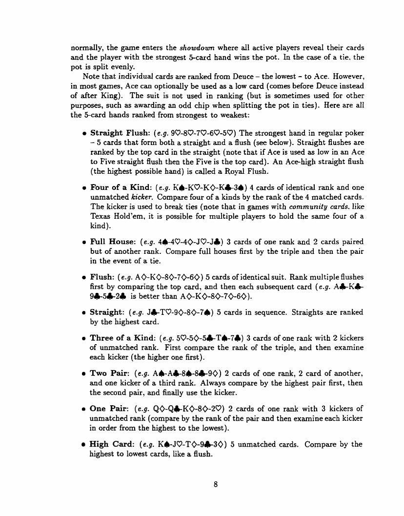
normally, the game enters the showdown where dl active players reveal their cards and the player with the strongest jcard hand wins the pot. In the case of a tie. the pot is split evenly.

Note that individual cards are r d e d from Deuce - the lowest - to Ace. However, in most games, Ace can optionally be used as a low card (cornes before Deuce instead of after King). The suit is not used in ranking (but is sometimes used for other purposes, such as awarding an odd chip when splitting the pot in ties). Here are al1 the S-card hands ranked from strongest to weakest:

Straight Flush: ( e.g. 90-80-70-60-59) The strongest hand in regular poker - 5 cards that form both a straight and a flush (see below). Straight flushes are ranked by the top card in the straight (note that if Ace is used as low in an Ace to Five straight flush then the Five is the top card). An Ace-high straight flush (the highest possible hand) is cdled a Royal Flush.

Four of a Kind: (e.g. KI-KO-KO-K&3&) 4 cards of identical rank and one unmatched kicker. Compare four of a kinds by the rank of the 4 rnatched cards. The kicker is used to break ties (note that in games with cornrnztnify cards. like Texas Hold'em, it is possible for multiple players to hold the same four of a kind).

a Full House: (e.g. 44-40-40-50-56) 3 cards of one r a d and 2 cards paired but of another rank. Compare full houses first by the triple and then the pair in the event of a tie.

Flush: ( e-g. AO-KO-80-70-60) 5 cards of identical suit. Rank multiple flushes first by comparing the top card, and then each subsequent card (e .9 . A&K& 9 & 5 6 2 4 is better than AO-KO-80-70-60)-

a Straight: (e.g. J(C-TO-90-8+?4) 5 cards in sequence. Straights are ranlied by the highest card.

a Three of a Kind: (e.g. 50-50-5&T&7&) 3 cards of one rank with 2 kickers of unmatched rank. First compare the rank of the triple, and then examine each kicker (the higher one first ) .

Two Pair: (e.g. AI-A*8@8&90) 2 cards of one rank, 2 card of another, and one kicker of a third rank. Always compare by the highest pair first, then the second pair, and finally use the kicker.

a One Pair: (e.g. QO-QCKO-80-20) 2 cards of one rank with 3 kickers of unmatched rank (compare by the rank of the pair and then examine each kicker in order from the highest to the lowest ).

High Card: (e-g. KI-JO-TO-9430) 5 unmatched cards. Compare by the highest to lowest cards, like a flush.

Some variants of poker recognize other special hand types (e-g. l-card flush) and allow wild cards (cards that can represent any other card). but these are not common in casino games.

2.2 Texas Hold'em The specific variant under consideration in this thesis is Texas Hold'em, the most popular variant played in casinos. It is used in the main event of the annuai World Series of Poker championship to determine the World Champion. It is considered to be one of the most strategically complex poker variants and has "the smallest ratio of luck to skill" [2]. The script for Texas Hold'em is as follows (each of the four rounds is followed by betting):

Pre-pop: each player is dedt two face-down cards (hole cards).

Flop: 3 cards dealt face-up to the board (community cards).

Turn: 1 card dealt face-up to the board.

River: 1 card dedt face-up to the board.

After the betting on the river, the best 5-card hand forrned from the two hole cards and five board cards wins the pot.

Specifically, we examine the game of Limit Texas Hold'em with a structured betting system of - 2 4 4 units, and blinds of 1 and 2 units. This rneans that the bet size is fixed at 2 (the small bet) for the pre-flop and flop, and 1 (the big be t ) for the turn and river. Before the pre-flop, the first player after the button is the small blind and is forced to put 1 in the pot, and the subsequent player is the big blind and forced to bet 2 (meaning the amount to c d is 2 for al1 subsequent callers, 1 for the small blind, and if there has been no raise, the big blind has the option to fold, check or raise to 4 units). Limit Hold'em is typically played with 8 to 10 players, although the minimum is 2 and possible maximum is 23.

In later chapters, we use a special convention for representing Texas Hold'em hands. The designation 80-J0/4&5&6& represents hole cards of 80-50 with a board of 4&5)6&.

Chapter 3

How Humans Play Poker

There have been many books written on how to play poker. However, these are intended for the development of human players and must be reinterpreted to be applicable to cornputer play. The author typically presents a small number of rules for human players to fdlow. These rules are frequently based on experience and sometirnes d s o have a mathematical foundation. For example, in his book, Norman Zadeh uses mathematical analysis to deduce a series of generalized rules for several poker variants [l5]. His rules al1 basically follow the form of giving the reader a threshold hand type to take a certain action in a certain situation.

Two of the more useful books for the purposes of this thesis are [14] and [13]. The first book, Hold 'em Poker for Aduanced Pla yers by David Sklansky and Mason Malmuth, presents a high-ievel strategy guide for the game of Texas Hold'em (which only recently has become the focus of poker literature), with a special treatise on playing the pre-flop. It presents a strong de-based approach with an emphasis that knowledge of your opponent should always be taken into account. The second book, The Theory of Poker by David Sklansky, is described by Darse Billings as "the first book to correctly identify many of the underlying strategic principles of poker" [-] and uses illustrated examples from several variants includjng Texas Hold'em. In this chapter, some of the more important concepts and strategies are described.

3.1 Hand Strength and Potential A human player should be able to estimate the probability that a certain set of cards will win. This is irnplicit in the rule-based systems which give threshold hands for betting decisions.

There are two different measures for the goodness of a hand: the potential and the strength. Potential is the probability that the player's hand will become the likely wiming hand (a 4 card flush counts for nothing but is very strong if a fifth suited card is dealt). It can easily be roughly estimated by humans - good players are usually able to estimate a hand's potentiai accurately, in t e m s of outs: "the number of cards left in the deck that should produce the best hand" [14]. In contrat , strength is the probability of currently being in the lead (would win if no further cards were dealt).

This is often based on experience or knowledge of the statisticd distribution of hand types, although knowledge of one's opponents is used by expert players to get a much more accurate estirnate-

Knowing where one stands with respect to these measures is used to determine an appropriate strategy, such as raising to reduce the number of opponents, trying to scaxe one's opponents into folding by betting aggressively, and so on.

3.2 Opponent Modeling The better players are at understanding how their opponents think, the more suc- cessfd they will be. Experts axe very good at characterizing their opponents and exploiting weaknesses in their play, and knowing when they do or do not have the best hand. They often try to put an opponent on a certain range of hands (guess the cards they hold) based on observed actions. It is important to note here that, if a player wins a game uncontested (no showdown), they do not have to reveal their cards. The showdown (exposure of an opponent's hidden cards) gives away information that can be used with the betting history to infer the decision-making process.

To take a less specific approach, one can estimate probabilities for a generic (or "reasonable") opponent. However, observing an opponent's play may give you useful information that allows you to bias the probabilities, allowing for more infonned (and more profitable) decisions. For example, an observant player is less likely to take a bet seriously from someone who bets aggressively every game. Good opponent modeling is vital to having a good estimate of hand strength and potential.

3.3 Position

Another variable expert players take into account for a betting decision is their p c ~ sition at the table with respect to the dealer (how many players have acted before you and how many act after you). In [14] the authors emphasize that a later position is better because you have more information available before you must make a decision. Their pre-flop strategy is dependent on a player's expected position in the later betting rounds. For example, they discusç a tactical raise, cdIed "buying the button", which is used in late position in the pre-flop to hopefully scare away the players behind you to becorne the last player to act in future betting rounds.

3.4 Odds This is a fundamental concept introduced in [13] and includes pot odds, effective odds, implied odds and reverse implied odds. Odds gives you a way to compare your cost versus the potential winnings, and determine how good of a hand, in terms of potential or strength, you require to cal1 a bet (or what the expected return is for each of your possible actions).

3.4.1 Pot Odds Also called immediate odds, pot odds are the ratio of money in the pot against the cost to d l . For exarnple, if there are $12 in the pot and it costs $4 to call then you are getting 3-te1 odds (winningsto- 'cost to çtay in "). This can be translated to a percentage, representing the size of your contribution in the new pot, by using the following formula:

"winnings cos t

( p o t s i t e + cost) '

This percentage is the required probability of winning. If you are on the final round of betting then these are the odds you should have of winning the hand.

Continuing the exarnple, the required probability is 4/(12 + 4) = 0.25. Hence, you need at least a 25% chance of winning to warrant a c d . For example, if your hand was 4 0 - 8 0 and the board was 70-AO-6&KO you would have a four-card diamond flush on the turn. kou would estimate having 9 outs of the remaining 16 cards to make a winning diamond flush. This translates to a hand potential of 9/46 = 0.196 so it would be incorrect to c d . On the other hand, you also have an inside straight draw (any 5 would give you a straight) and this is an additional 3 outs (the 5 0 has dready been counted). Now your potentiai is 12/46 = 0.261 so it is correct to call.

However, there are several caveats. Simply making the call does not necessarily end the round in a multi-player scenario; if there is a player behind you who has yet to see the bet , they may raise. In the above example, if you were expecting the player behind you to raise another $4 and the original bettor to call, then your pot odds are now 540-2 (pay $8 to win $20), elevating the threshold for staying in the hand to 8/(20 + 8) = 286. Also, knowledge of your opponents is not only required for an accurate estimate of hand strength or potential, but also to determine if you can expect to have to pay more. When considering potential this also assumes that the cards you are hoping for will make your hand the winner and not the second best. Further complications a ise when there is more than one card left to be dealt.

3.4.2 lmplied Odds and Reverse Implied Odds

Implied odds (and reverse implied odds) are based on the possibility of winning (or losing) more money later in the hand. They consider the situation after the next cards have been dealt and explain situations where things are better (or worse) than pot odds make them seem. Put another way, implied odds is the ratio between the amount you expect to win when you make your hand (more than what is in the pot) versus the amount it will cost to continue playing. In contrast, reverse implied odds is the ratio between the amount in the pot (what you win if your opponent does not make their hand) venus what it will cost you to play until the end of the haad. One of the major factors behind considering implied odds is how hidden your hand is (how uncertain your opponent is of your hand); another is the size of future bets. For the latter reason, implied odds become more important in no-limit and pot-limit games than in fixed-Iimit games.

As an example of implied odds. consider that at the tum there is $12 in the pot. it is $4 to cd1 (pot odds 3-tel), hitting your hand means you very likely will win. and additionally your opponent is likely play to the showdown. If you miss you will simply fold (costing $4). If you hit you can expect to make an extra bet of 94 from your opponent, winning $16 total so your implied pot odds are 4-tel.

For reverse irnplied odds, consider that you have a strong hand but little chance of improving and your opponent has a chance of irnproving to a hand stronger than yours, or possibly already has a hand stronger than yours (they have been betting and you are not sure if they are bluffing) - essentially a situation where you are not certain that you have the best hand. Say it is the turn and there is $12 in the pot and it is $4 to cal1 (pot odds % t e l ) . If your opponent has a weak hand or misses their card they may stop betting in which case you would only win $12 (it costs $4 to find out you are winning). Otherwise, you have committed to playing to the end of the hand in which case it would cost you $8 to find out you are losing (pot odds 3-te2). There are many variations to this scenario. The essential idea is that reverse implied odds should be considered when you are not certain you have the best hand; it will cost more in future betting rounds to discover this.

3.4.3 Effective Odds When you are considering the odds of making your hand with two cards remaining, it is difficult to estimate the expected cost to play those two rounds. For example, if there is $6 in the pot after the flop and your single opponent has just bet 82, then your pot odds are %te l . However, you have two cards to make your hand so you must try to estimate the cost of the next round. Against a single opponent the worst case is that your opponent will bet next round and you will simply c d ; you would be paying $6 to win $10 (540-3) which increases the requirement for playing.

However, since you have two chances to make your hand your potential will improve as well. If you held 40-80 and the board was 70-AO-64, your estimated chance of hitting the flush or the inside straight (12 outs) after two cards is now 12/47 + 35/47 * 12/46 = .45, making it correct to cal1 (or possibly raise) a bet on the 00p.

3.5 Playing Style

There are severd different ways to categorize the playing style of a particular player. When considering the ratio of raises to calls a player may be classified as agressive, moderate or passive. Aggressive means the player frequently bets or raises rather than checking or c a n g (more than the nom), while passive means the opposite. Another simple set of categories is loose, moderate and tight. A tight player will play fewer hands than the nom, and tend to fold in marginal situations, while a loose player is the opposite. Players may be classified differently for pre-flop and post-flop

play-

3.6 Deception and Unpredictability

A predictable player in poker is generally a bad player. Consider a player who never bluffs (when that player bets, they always have a strong hand). Observant opp* nents are more likely tu fold (correctly) when this player bets, reducing the winning pot size. Of course, against weak, unobservant opponents, never blding may be a correct strategy. However, in generd, deception and unpredictability are important. Although the cost and benefit of such actions must be considered, unpredictability can be achieved by randomly mixing actions. For exarnple, do not raise every time you hold a high pair before the flop, otherwise an observant opponent can assume you are not holding a high pair when you simply cal1 in the pre-flop. Deception is more cornplex and can be achieved through numerous different high-level strategies. Following are some of these strategies.

0 Changing Styles: is a simple form of deception to deliberately create false impressions. For example, early in the session you might play a tight conservative style and show a lot of winning hmds at the showdown. Later you switch to a looser style, and observant players are likely to continue to treat you as a tight player and take your bets very seriously.

Slowplaying: ' ... is playing a hand weakly on one round of betting in order to suck people in for later bets* [13]. Checking or cdling in an earlier round of betting shows weakness, and this hopefully leads to your opponents being willing to put money in the pot later in the hand (particularly in those variants of Hold'em where the bet size doubles in later rounds). However, since you will often be up against many opponents, you need a very strong hand for this kind of play.

Check-raising: is another way to play a strong hand weakly. Sklansky calls it a way to "trap your opponents and win more money from them" 1131. Essentially you believe that had you opened betting in the round you would either drive out players or only get one bet (no one would raise). But if you believe that one of your opponents will open the betting you begin the round by checking. Assuming the opening bet is then made, you follow by raising. Hopefully, players who have dready put in a bet are willing to put in a second. However, even if players fold you still have their money from the opening bet.

Bluffing: is an essential strategy in poker. It has been mathematically proven that you need to over-play or under-play (bluff or slowplay) in some way for optimal play in simplified poker (111. Bluffing d o w s you to rnake a profit from weak hands, but it also creates a false impression which will increase the profitability of hiture hands (a lot of money con be won when betting a very strong hand and your opponent suspects you may be bluffing). In practice, you need to be able to predict the probability that your opponent will cal1 in order to identify profitable opportunities. A game-theoretic exphnation of the optimum bluffing frequency is presented in [13].

0 Semi-bluffing: is a bet with a hand which is not likely to be the best hand at the moment but has a good chance of outdrawing calling hands (e-g. a four- card-flush). On occasion this play will also win outright when your opponents fold. The combined chances of winning immediately, or improving when called, makes it a profitable play.

Note that sometimes deception can be used to play an action which does not necessarily have the largest expected value, but rather creates a false impression which may indirectly lead to returns in the fùture. While undoubtedly important, it is difficult to rneasure the effectiveness of this type of deception.

3.7 Summary

The short term goal in poker (the goal in a specific deal) is either to maximize your gain if you think you can win (either with a strong hand or by bluffing with a weak hand) or to minimize your loss if you think you will Iose. However, the outcomes of individual games are not independent. You can afford to make some 'bad moves' (the expected value for the chosen action in the current game is not the highest) provided they contribute to greater gains in later games.

An expert player is one who can usually recognize when they have or do not have the winning hand, and c m maximize the money they win appropriately. They also occasionally invest money in misinformation (such as bluffing) and have the ability to identify good hands and understand their opponents (how they will react to certain actions or what hand they likely hold based on their actions). Knowledge of tells (physical mannerisms) and psychological plays are sometimes used in :he human side of opponent modeling. Overall, the expert player has a good understanding of playing strategies, hand strength and potential, pot odds, and good opponent modeling skills. These factors are used as the basis for every decision made.

Chapter 4

How Cornputers Play Poker

Very little work has been done on poker by computing scientists, although there are numerous commercial and hobbyist approaches. The w i o u s computer-based approaches to poker can be classified into three high-level architecture descriptions (or a mixture thereof): expert system, garne-theoretic optimal play, and simulation / enurneration-based systems. Each of these will be discussed in the following sections.

This chapter will also discuss several case studies of programs by computing scientists and hobbyists. Included in the former group is the historical work of Nicolas Findler dong with the more recent ideas of Daphne KoUer and Avi Pfeffer. Findler worked on a poker-playing program for 5-card draw poker (61. Kolier and Pfeffer implemented the first practical algorithm for finding optimal randomized strategies in tweplayer imperfect information games [IO]. Among the hobbyist approaches examined are several that play poker on an online poker server over IRC (Internet Relay Chat). Three of these programs are r00160t, replicat and zbot (although variations of these sometimes run under different names). Additionally there are two public domain programs: Smoke'em Poker for Microsoft Windows, as well as Seven-Card Stud and Texas Hold'em implementations by Johann Ruegg for the UNIX curses package. There are numerous approaches by commercial companies, although only a few have a target audience of professional players. The best of these is Turbo Tezas Hold'em by Wilson Software (http://www.wiIsonsoftware.corn). It is an extremely nile-based system.

The final section discusses the architecture selected for our poker player and the reasons behind the selection.

4.1 Expert Systems

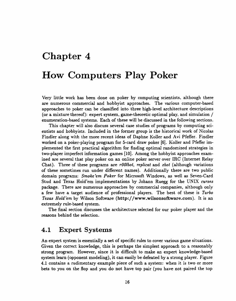
An expert system is essentidy a set of specific d e s to cover various game situations. Given the correct knowledge, this is perhaps the simplest approach to a reasonably strong program. However, since it is difficult to make an expert knowledge-based system learn (opponent modeling), it can easily be defeated by a strong player. Figure 4.1 contains a rudimentary example piece of such a system: when it is two or more bets to you on the Bop and you do not have top pair (you have not paired the top

PlayFlop(CARDS myhand, STATE state)

{ if (state. bets+utin==O)

kk state.bets20-cal1 > I && myhand < TOPSAIR && myhand ! =FOURILUSH 08 myhand ! =OPENSTRAICET)

retarn SelectAct ion(RAISE, IO, CALL, IO, FOLD 8 0 ) else . . -

Figure 1.1 : Example of an Expert Knowledge-Based System

card on the board and do not have a hole pair bigger than that card), nor do you have a four card flush or an open-ended straight, then raise 10% of the time, cal1 10% of the time, and fold 80% of the time.

There are many problems with this type of approach. Clearly, covering enough of the situations that will arise in practice would be very laborious. Also such a system is difficult to make flexible. If the system were made specific enough to be quite strong, conflicting rules could possibly be constmcted and there would need to be a way to handle exceptions. Missing d e s covering certain situations or making the rules too general would make the program weak and/or predictable. Additionally, you need an expert who can define these d e s . This knowledge-acquisition bottleneck may prove to be a serious probiem.

4.2 Game-Theoret ic Optimal Strategies

Kuhn [Il] along with Nash and Shapley [12] have demonstrated that "optimal strategies" using randomization exist for simplified poker. An optimal st rategy always takes the best worst-case move, and this means two things: "the player cannot do better than this strategy if playing against a good opponent, and furthemore the pIayer does not do wone even if his strategy is revealed to his opponent" [IO]. For example, consider the tweplayer game of Roshambo (Rock, Paper, Scissors). The optimal strategy is to select a move uniformly at random ( i. e. [i, ?, $1) irrespect ive of the game history.

Finding an optimal approach is not so easy in a complex game Like poker; there is a major stumbling biock. Due to the enormous branching factor ( s e Figure 4.2), bot h the calculation and storage of the game-theoretic optimal strategy would be extremely expensive. Additionally the branching factor numbers are only for the two player environment - the mdti-player environment is even more complex due to the addition of more imperfect information and many more possible betting interactions. As demonstrated by the attention devoted to multi-player situations in the poker literature, such considerations are quite important.

Additionally, the gamet heoretic optimal approach is not necessarily the best .

Clearly, as the garne-theoretic optimal strategy is fixed, it cannot take advantage of observed weaknesses in the opponent. Doing so would risk falling into a trap and losing. Consider Roshambo for an example. After witnessing your opponent playing Rock 100 times in a row, deciding to play Paper risks your opponent anticipating your action (the situation rnay be intended as a trap or your opponent may know your strategy). The existence of the risk, no matter how srnall, would violate the optimality of the strategy (the second guarantee, that the player cannot do worse).

Because of this, even against bad players an optimal strategy is likely to only break even. In contrast, a maximal strategy using opponent modeling (which does not assume perfect play from its opponents) would identify weaknesses and exploit them for profit (significantly more than an optimal strategy). There is some risk, because deviation from the optimal opens the door for your opponent to exploit it. But, if your knowledge of the opponent is good, the potential gains outweigh the risk. A game-theoretic optimal st rategy would, however, make an excellent default or baseline to complement such an "adaptive" strategy.

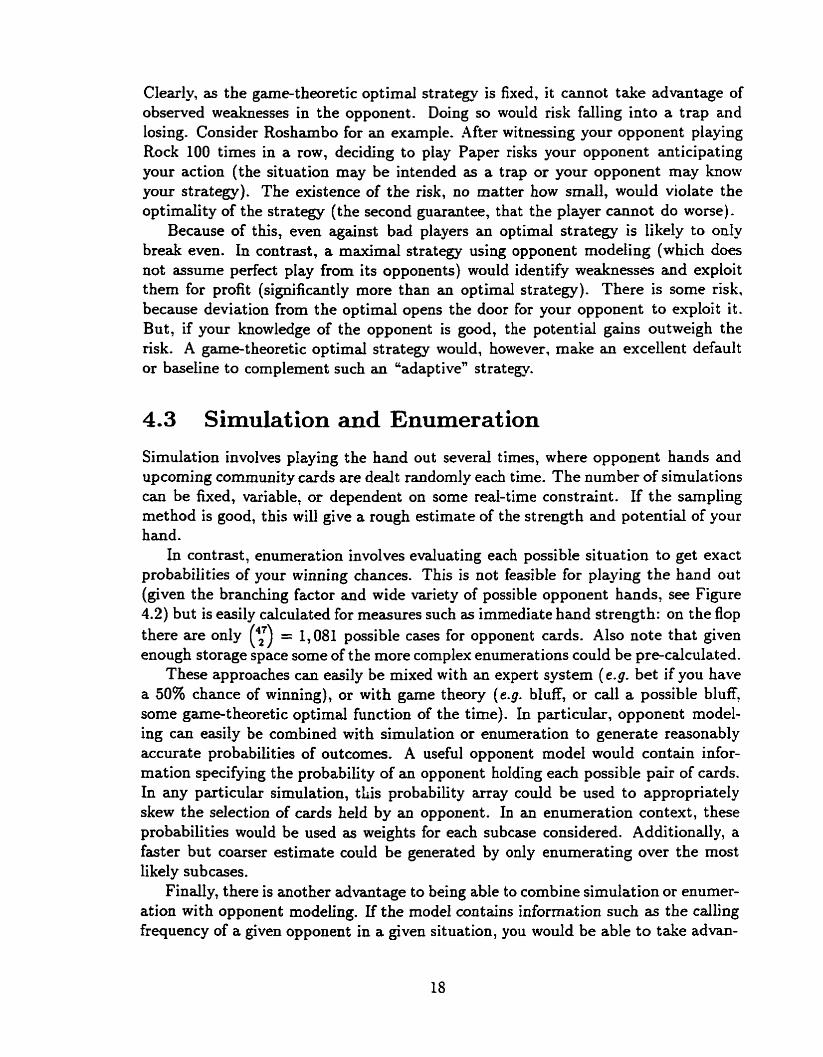
4.3 Simulation and Enurneration

Simulation involves playing the hand out several times, where opponent hands and upcoming community cards are dealt randomly each time. The number of simulations can be fixed, variable, or dependent on some real-time constraint. If the sampling method is good, this will give a rough estimate of the strength and potential of your hand.

In cont rast , enumeration involves evaluat ing each possible situation to get exact probabilities of your wiming chances. This is not feasible for playing the hand out (given the branching factor and wide variety of possible opponent hands, see Figure 4.2) but is easily calcuiated for measures such as immediate hand strength: on the flop there are only (42') = 1,081 possible cases for opponent cards. Alço note that given enough storage space some of the more complex enurnerations could be pre-calculated.

These approaches can easily be rnixed with an expert system ( e.g. bet if you have a 50% chance of winning), or with game theory (e.g. bluff, or cal1 a possible bluff, some gamet heoretic optimal function of the tirne). In particular, opponent modeling can easily be combined with simulation or enumeration to generate reasonably accuate probabilities of outcomes. A useful opponent model would contain information specifying the probability of an opponent holding each possible pair of cards. In any particular simulation, tliis probability array could be used to appropriately skew the selection of cards held by an opponent. In an enumeration context, these probabilities would be used as weights for each subcase considered. Additionally, a faster but coarser estimate could be generated by only enumerating over the most Li kely subcases .

Finally, there is another advantage to being able to combine simulation or enumeration with opponent modeiing. If the model contains information such as the calhg frequency of a given opponent in a given situation, you would be able to take advan-

Assuming only two players:

0 2 possibilities for who acts first

(7) = 1,326 different hole cards

0 (y) t 47 * 46 = 42,375,200 significantly different ways the board can be dealt ( (y ) difTerent flops, 47 dXerent tum cards, 46 different river cards)

0 15 different ways the betting can proceed in the pre-flop (ody 7 do not end in one side winning uncontested)

O 19 different ways the betting can proceed in any round after the pre-flop (only 9 do not end in one side winning uncontested)

Therefore: . 2 r (:? * 7 * (y) = 363.9 * 106 different states at the beginning of the Bop

s 363.9 * loS * 9 * 47 = 153.9 * log different states at the beginning of the turn

O 153.9 * log * 9 * 46 = 63.7 * 1012 different states at the beginning of the river

O Also note there are up to (';) possible opponent han& a t each stage in the game (n = 50 for the pre-%op, 47 for the fîop, 46 for the turn, and 45 for the river). This hidden information was not inchded in the above products (which are the number of possible variations of known information).

This is still a large tree even though there is some redundancy in the way the car& are dealt (suits are isomorphic) :

O 169 significantiy diff'erent classes of hole cards rather than 1,326 (see Appendix A). This reduces the number of states at the beginning of the flop to 46.4 * 106, and 8.1 * 10'' a t the beginning of the river (approximately a 7.8-fold reduction).

O An additional complex reduction based on the isornorphism of suits can reduce the original number of possible flop states and starting hands from 1326 * (3) = 26.0 * 106 (3.3 * 10' with the elhination of redundant starting hands) to 1.3 * 10' (approximately an additional 2.5-fold reduction - still leaves a large number at the river). The details of the reduction are not presented here. It is based on enumerating each possible combination of suits in the starting haod and on the flop. For example, there are only (:3 = 78 significantly different starting bands where both car& are of the same suit (map this suit to, say, 4), and there are only 11 * (If) = 858 signikantly different flops where one card is of the original suit (mapped to 4) and the other two cards are of a second suit (mapped to, Say, 0).

The addition of multi-player considerations exponentially complicates the tree:

O three players in any round after the pre-flop: 138 sequences of betting actions end with two players remaining and 46 end with three players rernaining (93 end in an uncontested win). For two players there were only 9 different quences that did not terminate the gome instead of 184.

O four players on any round after the pre-flop: 1504 sequences of betting actions end with two players remaining, 874 end with three players remaining, and 161 end with all four players remaining (792 end in an uncontested win).

Figure 4.2: Branching Factor for Structured Bet ting Texas Hold'em With a Maximum of 4 Bets/Round

tage of a more realistic consideration of some outcornes. For example. consider the situation where you are at the river against one opponent, the pot contains 020. and your options are to check or bet $4. Given the probability m a y of your opponent's model you calculate by enurneration that you have only a 10% chance of having the stronger hand. The mode1 tells you that, when faced by a check in this situation. your opponent will check 100% of the time, and faced by a bet your opponent will fold 30% and call 70%. You can therefore calculate the expected value ( E l / ) of your two options:

check: win $20 10% of the tirne, lose $0 90% of the time.

EV = 20 * 0.10 - O * 0.90 = 2.00-

bet: since p u r opponent will likely fold the weakest 30% of hands, and p u could only beat 10% of al1 hands (or the worst third of the hands they fold) then there is no chance that you win if they call.

- opponent folds 30%: win $20 100% of the time.

- opponent calls 70%: \vin $24 0% of the time, lose 84 100% of the time.

EV = 0.30 * (20 * 1.00) + 0.70 * (24 * 0.00 - 4 * 1.00) = 3.20. Therefore, it is more profitable if you bet (due to the reasonable possibility of scaring your opponent into folding).

This is a simple contrived example but it demonstrates how well an accurate opponent model compiements a simulation or enuneration system.

4.4 Findler's Work Nicolas Findler worked on and off for 20 years on a cognition-based poker-playing program for Five-Card Draw [6] [7] [8]. He recognized the benefits of research into poker as a model for decision-making with partial information. However, much of the applicability of his work to ours is lost due to differing goals; rather than being con- cerned about producing a high performance poker program, he focused on simulating the thought processes of human players. Hence, to achieve this, instead of relying heavily on mathematical analysis, his approach was largely based on rnodeling human cognitive processes. He did not produce a strong poker player.

4.5 The Gala System

A more theoretical approach by computing scientists was taken by Koller and PfeEer [IO]. They implemented the first practical algorithm for finding optimal randomized strategies in two-player imperfect information cornpetitive games. This is done in their Gala system, a tool for speciS.ing and solving problems of imperfect information. Their system buiids trees to find the garne-theoretic optimal (but not maximal)

strategy. However, even when considering only the two-player environment. only vastly simplified versions of poker can presently be solved, due to the large size of trees being built. The authors state that "... we are nowhere close to being able to solve huge games such as full-scale poker, and it is unlikely that we will ever be able to do so."

4.6 Hobbyists

Several programs by hobbyists were exarnined to explore the architecture and a p proach used. The most common approach is expert-based, however simulation- based approaches tend to be stronger (dthough more computationally expensive).

xbot by Greg Reynolds uses an expert system which is manually patched when weakness is observed.

a replicat by Stephen How also uses an expert system in combination with observing a large number of possible features about the hand and board (e.g. three-straight ).

rOOlbot by Greg Wohletz is perhaps the strongest of the three IRC programs. For the pre-flop it uses Sklansky and Malmuth's recornrnendations (141, and for the post-flop it conducts a series of simulations (playing out the hand to the showdown, typicdy 3,000 times) against N random hands (where N is the number of opponents, and is artificially adjusted for bets and raises). The actual action is dependent on what percentage of simulations resulted in a win.

0 Smoke'em Poker is a Five-Card Draw program by Dave O'Brien. It uses an expert system and has a set of d e s for each opponent type (e.g. tight. loose).

There are two poker gomes by Johasn Ruegg, Sozobon Ltd. Both the Seven- Caxd Stud and Texas Hold'em games use a simulation-based approach where the program plays the hand to the showdown several times against random opponent S. The resulting winning percentage is artificially adjusted depending on the game state and compared against several hard-coded action thresholds.

4.7 Architecture

Consideration of these other programs and the various advantages of the different approaches led us to select a primarily enurneration-based approach for the purposes of this thesis. There were several reasons:

The expert system is too limited and context sensitive ( the game is far too complex to cover all possible contexts). It also is inflexible, and will inherit any error in the designer's approach to the problem.

The game-theoretic optimal strategy is very complex to compute =dl if such a system could be built, presumes optimal play on the part of the opponents. We are working under the assumption that Our opponents will make errors and therefore maximal play is preferable.

An enurneration-based approach is easy to combine with an opponent modeling system based on the probability distribution of possible opponent holdings.

Most of the desired values are computationally feasible in real-time. Where this is not sol there are many ways to calculate good approximations of the mesures (e.g. random simulation, pre-computation, heuristics).

a Values calculated by enurneration (as opposed to simulation) are more accurate since random sampling introduces variance, and rule-based systems are subject to systemic error.

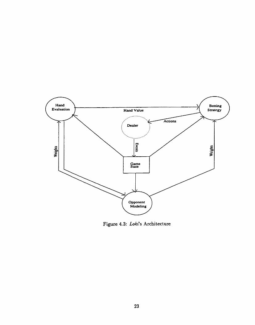
Loki (Figure 4.3) is a complete poker-playing program (able to play a full game of Texas Hold'em unaided). There are three main cedependent components which control the play of the program. These components are discussed in the following chapters. They are hand evaluation (using the opponent models and game state, it generates values which roughly correspond to the probability of holding the strongest hand), betting strategy (it uses the values generated by hand evaluation, the o p ponent rnodels, and the game state to determine the best action), and opponent modeling (it translates the betting history of the opponent into information about betting behavior and possible hands held).

4.8 Summary

Three main approaches to program design were summarized in this chapter: the expert system (hard-coded rules based on the knowledge of an expert), game-theoret ic optimal strategies, and simulation/enumeration-based. The first two approaches have some obvious limitations. However, the different approaches can be combined to various extents.

While there are many poker-playing programs, none are very strong, and few make source code or a description of the imer workings available. Also, with the exception of Findler and Koller/Pfeffer there are few resources in the computing science literature. There is dso little on building a high-performance poker P ~ O ~ ~ I I I , except for some ideas presented in [2].

Opponcnt Modeling

Figure 4.3: Lokà's Architecture

Chapter 5

Hand Evaluation

Accurate assessrnent of your winning chances is necessary when considering the cost of playing versus the payoff with pot odds. Hand evaluation uses the opponent models and garne state to calculate estimates of the winning chances of your hand. However, since there are more cards to corne on the flop and tuni, the present strength of a band is insufficient information. For this reason, post-flop hand evaluation is broken into two parts: strength and potential. Strength is the probability of a hand c u m n t l y being the strongest and potential is the probability of the hand becoming the strongest (or of losing that status to another hand) after future cards have been dealt. Due to the computational complexity of potential for the pre-flop (the first two cards), evaluation in this stage of the game is given special treatment.

5.1 Pre-Flop Evaluation

Hand strength for pre-flop play has been extensively studied in the poker literature. For example, [14] attempts to explain strong play in human understandable terms. by ciassifying ail the initial twecard pre-flop combinations into nine betting categories. For each hand category, a suggested betting strategy is given, based on the strength of the hand, the number of players in the game, the position at the table (relative to the dealer), and the type of opponents. For a poker program, these ideas could be implemented as an expert system, but a more generd approach wouid be preferable.

For the initial two cards, there are (y) = 1,326 possible combinations, but only

169 distinct hand types (13 paired hands, (y ) = 78 suited hands and 13 * (2) = 78 unsuited hands). For each one of the 169 possible hand types, a simulation of 1,000,000 games was done against each of one, three and six random opponents (to cover the 2, 3-4 and 5 or more player scenariosl). Each opponent was simple and always called to the end of the hand. This produced a statistical mesure of the approximate income rate ( IR) for each starting hand; income rate mesures the retum on investment .

nethankroll I R =

hands-pla yed

'We consider these the most important groupings. See Appendix B.

The computed values are presented in Appendix -4. These numbers must always be viewed in the current context. They were obtained using a simplifying assumption, where the players aiways c d to the end. However, this experiment gives a good first approximation of how strong a hand is. For example, in the 7-player simulation the best hand is a pair of aces and the worst hand is a 2 and 7 of different suits. While the absolute I R value may not be useful, the relative order of the hands is. As we discuss in Appendix A, there is a strong correlation between these simulation results and the pre-flop card ordering given in [Ml.

Hand Strength

Hand strength assesses how strong your hand is in relation to what other players may hold. Critical to the program's performance, it is computed on the flop, turn and river by a weighted enumeration which provides an accurate estimate of the probability of currently holding the strongest hmd. This calculation is feasible in real-time: on the flop there are 47 rernaining unknown cards so (''21) = 1,081 possible hands an . . opponent rnight hold. Similarly there are ('2) = 1,035 on the turn and (42) = 990 on the river.

Figure 5.1 contains the algorithm for computing hand strength. The bulk of the work is in the cal1 to the hand identification function Rank which, when given a hand containing at least 5 cards, determines the strongest 5-card hand and maps it to a unique value such that stronger poker hands are given larger values and hands of equal strength are given the same value. Rank must be called (r) + 1 times where n is the nurnber of unknown cards.

The parameter w is an array of weights, indexed by two card combinations, so the function determines a weighted sum. It is the weight a m y for the opponent under consideration (each possible twwcard holding is assigned a weight ). When the array is normalized so the sum is 1, the weights are conditional probabilities meaning "for each possible twecard holding what is the probability that it is the hand held by this opponent" (given the observed betting). Without n~rmalization~ the values in the weight table are conditional probabilities meaning Uwhat is the probability that this opponent would have played in the observed manner" (given they held this hand). Without opponent modeling, it can simply be fdled with a default set of values, either a uniform or 'typical' distribution. Under uniform weighting eadi entry in the m a y is equal (an appropriate representation if the opponent has a random hand). A more typicd distribution would be a set of values based on the I R tables. This is the only mode1 information used directly by the hand strength enumeration.

Suppose our start ing hand is A+Q+ and the flop is 30-4+JO (1,081 possible o p ponent hands). To estimate hand strength using uniform weighting, the enumeration technique gives a percentile ranking of our hand (our hand rank). We simply count the number of possible hands that are better than ours (any pair, two pair, A-K, or three of a kind: 444 hands), how many hands are equd to ours (9 possible rernaining A-Q combinations), and how many hands are worse than ours (628). Counting ties as

HandStrength(CARDS ottrcards,

RANK ourranir, opprank CARDS oppcards FLOAT ahead, tied, behind,

CARüS boardcards , FLOAT an )

handstrength

ahead = t i e d = behind = O ourranh = Rank(ourcards. boardcards ) /* Consider al1 two card combinations of the remaining cards */ f o r each case(oppcards )

opprank = Rank(oppcards, boardcards) if (oarrank>opprank) ahead += ~Coppcards] e lse if (ourrank==oppranh) t i e d += u [oppcards] else /* c */ behind += a [oppcards]

1 handstrength = (ahead+tied/2) / (ahead+tied+behind) return (handstrength)

1

Figure 5.1 : HandS trength Calculat ion

half, this corresponds to a hand rank (HR) of 0.585. In other words there is a 5S.% chance that Our hand is better than a random hand (against non-uniform weights we cal1 it hand strength, or HS).

This mesure is with respect to one opponent, but when al1 opponents have the sarne weight array it can be roughly extrapolated to multiple opponents by raising it to the power of the number of active opponents (HR, is the hand rank against n opponents, HR m H R 1 ) .

H R , = ( H R I ) " . (5.2)

It is not an exact value because it does not take into account interdependencies arising from the fact that two players cannot hold the same card. However, this is a secondary consideration.

Continuing the example, against five opponents with randorn hands the adjusted hand rank is HSs = .5855 = .069. Hence, the presence of additional opponents has reduced the likelihood of our having the best hand to only 6.9%.

This example uses a uniform weighting: it assumes that aU opponent hands are equally Likely. In reality this is not the case. Many weak hands like 404, (1 R < 0) would have been folded before the flop. However, wit h the example flop of 30-4CJO, these hidden cards make a strong hand that skews the hand evaluations. Specifically, accuracy of the estimates depend strongly on models of our opponents (the array of weights w ) . Therefore, we compute weighted sums to obtain hand strength (HS). As with H R, HS, is the hand strength against n opponents and HS HSl.

5.2.1 Multi-Player Considerat ions

The above description of the weighted enurneration systern for hand strength is intended for one opponent. When the system was first put to use, the weight array was common to all opponents (either uniform or some fixed 'typical' distribution) so HS, was easily extrapolated by using Equation 5.3. However, our opponent modeling system will be cornputing a different set of weights for each specific opponent.

The correct approach would be to treat each possible case independently. For example, one possible case is that player 1 holds AO-QO and player 2 holds QU- J+. To handle this distinction, the function wodd need an extra iteration layer for each opponent (and would still be dependent on the order of the iteration). For each possible case it would then use a weight w [ t j = wl[xl ] * wz[x2] * --. * w,,[x,] (where I is the cornplex subcase, xi is the subcase for the cards held by player i and wi[xi] is the weight of that subcase for player 2 ) . The weight of the complex subcase given in the example is w[AO-QQ-QO-J,] = wl[AU-QQ] t w2[QU-JI] . The increase in computational complexity is substantial (approximately a factor of 1,000 for each additional player) and becomes infeasible with only 3 opponents.

There are two simpler methods to approach this problem and obtain good estimates of HS,. The first calculates HSp, for al1 opponents pi (such that i = 1.n) given each respective weight array. It then uses the equation

The second method calculates HSl using a special weight array, called the field a m y , computed by combining the weight arrays of al1 active players. HS, is then calculated with Equation 5.3. The use of the field array as an estimate is a compromise between computational cost and accuracy. It represents the entire table by giving the average weights of the opponents. The process of obtaining hand weights and generating this array is described in Chapter 7.

Both of t h n e methods are only estirnates because they ignore the interdependencies arising from the fact that two players cannot hold the same card. Several situations were examined from data gathered during play agaînst human opponents. For both methods, the absolute error was measured with respect to the correct full enurneration but only against two or three active opponents (four opponents was too expensive to cornpute). For the first method (Equation 5.4), this testing revealed the error never exceeded 2.19%. The average error was 0.307% with two opponents and 0.502% with three opponents. For the second method (using the field array and Equation 5.3), the error never exceeded 5.79% for two opponents and 4.15% for three opponents. In fact, for two opponents only 59 out of 888 cases had an error larger than 2% (and 20 out of 390 three opponent cases). The average errors were 0.671% and 0.751 %. The estimated values were usually slight overestimates.

This isolated test scenario suggests that the first method is better but the difference is srnall. The error dso appears to get siightly worse with additional opponents. Loki uses the second method due to the faster computation and ease of introduction into the present frarnework (particularly with respect to multi-player considerations

for hand potential, as will be discussed later). We have not invested the time to furt her explore the error arising from t hese interdependencies. however we believe it is minor in cornparison to the extra work that would be required for a very accurate measure of HS,. Also, this amount of error is considered to be negligible given that the error introduced by other components of the system tends to be greater in magnitude.

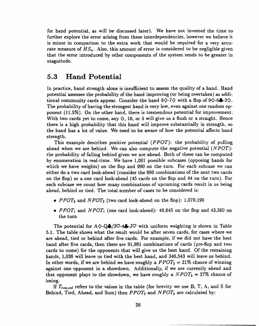
5.3 Hand Potential In practice, hand strength done is insufficient to assess the quality of a hand. Hand potential assesses the probability of the hand improving (or being overtaken) as additional community cards appear. Consider the hand 80-70 with a fiop of 90-6120- The probability of having the strongest hand is very low, even against one random o p ponent (11.5%). On the other hand, there is tremendous potential for improvement. With two cards yet to come, any 0, 10, or 5 will give us a flush or a straight. Hence there is a high probability that this hand will improve substantially in strength, so the hand has a lot of value. We need to be aware of how the potential affects hand strength.

This example describes positive potential (P P O T ) : the probability of pulling ahead when we are behind. We can also cornpute the negative potential (NPOT): the probability of falling behind given we are ahead. Both of these can be computed by enurneration in real-time. We have 1,081 possible subcases (opposing hands for which we have weights) on the flop and 990 on the turn. For each subcase we can either do a two card look-ahead (consider the 990 combinations of the next two cards on the flop) or a one card look-ahead (43 cards on the flop and 44 on the turn). For each subcase we count how many combinations of upcoming cards result in us being ahead, behind or tied. The total number of cases to be considered is:

PPOT2 and NPOT* (two card look-ahead on the flop): 1,070.190

PPOT1 and NPOT1 (one card look-ahead): 48,615 on the flop and 43,560 on the turn

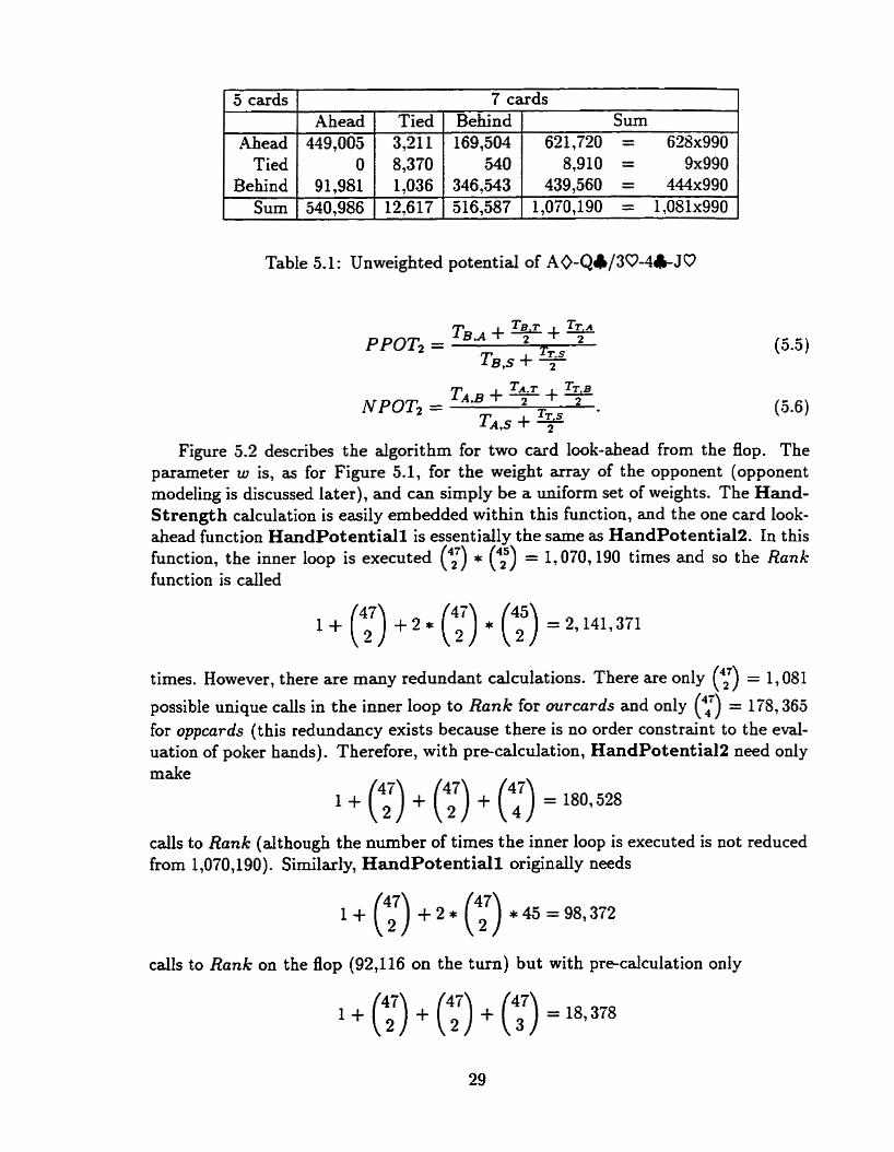
The potentid for AO-Q&/30-4&JO with unifmm weighting is shown in Table 5.1. The table shows what the result would be after seven cards, for cases where we are ahead, tied or behind after five cards. For example, if we did not have the best hand after five cards, then there are 91,981 combinations of cards (pre-flop and two cards to come) for the opponents that will give us the best hand. Of the remaining hands, 1,036 will leave us tied with the best hand, and 346,543 will leave us behind. In other words, if we are behind we have roughly a PPOT2 = 21% chance of winning against one opponent in a showdown. Additionaliy, if we are currently ahead and that opponent plays to the showdown, we have roughly a NPOT2 = 27% chance of losing.

If Trm,,i refers to the values in the table (for brevity we use B, T, A, and S for Behind, Tied, Ahead, and Surn) then PPOTz and NPOT2 are calculated by:

5 cards

Ahead Tied

Table 5.1 : Unweighted potential of AQ-Q4/30-4&J O

Behind Sum

Figure 5.2 describes the algorithm for two card look-ahead from the flop. The parameter w is, as for Figure 5.1, for the weight array of the opponent (opponent modeling is discussed later), and can simply be a uniform set of weights. The Hand- Strength calculation is easily ernbedded within this function, and the one card look- ahead function HandPotentiall is essentially the same as HandPotential2. In this function, the inner loop is executed (?:) * *(42) = 1? 070,190 tirnes and so the Rank function is called

7 caxds

tirnes. However, there are many redundant calculations. There are only r;) = 1, 081

possible unique calls in the inner loop to Rank for ourcards and only (?:) = 178,365 for oppcards (this redundancy exists because there is no order constra.int to the evaluation of poker hands). Therefore, with pre-calculation, HandPotential2 need only

91,981 540,986

make

Sum 621,720 = 628x990

8,910 = 9x990

c& to Rank (dthough the number of times the inner loop is executed is not reduced from 1 ,O?O,lgO). Similady, HandPotentiall origindy needs

Behind 169,504

540

Ahead 1 Tied

1,036 12,617

calls to Rank on the flop (92,116 on the tum) but with pre-calculation only

449,005 O

3,211 8,370

346,543 516,587

439,560 = 444x990 1 ,0701190 = 1,081~990

HandPoteatial2 (CARDS ourcards , CARDS boardcards , FLOAT w 0 ) {

/ * Each index represents ahead, t i e d and behind- */ FLOAT HP [31 C31 /* i n i t i a l i z e t o O */ FLOAT EiPtotal C31 /* i n i t i a l i z e t o O */ FLOAT ppot2, npot2 RANK oarrankS, oiurank7, opprank CARDS addit ionalboard INTEGER index

ourraab6 = Rank (oarcards , boardcards ) /* Consider al1 remaining t s o card combinations f o r the opponent */ fo r each case(oppcards)

/* aiter 5 cards */ opprank = Rank(oppcards , boardcards ) if (ourrank5>opprank) index = ahead e l s e if (ourranh5-oppranh) index = t i e d else /* < */ index = behind HPtotal [index] += P [oppcards]

/* Consider al1 possible tuo card board combinations t o corne */ for each case (addit ionalboard) {

board = boardcards + additionalboard 0rirrarih7 = ~ a P h (ourcards ,board) oppranl = Rank(oppcards board) if (ourranh7>oppraak) HP [index] Caheaa += o Coppcardsl e1se if (ourrank7=oppranL) BP [index] E t ied] += ri ~oppcardsl e l se /* < */ EiP [index] [ b e h i d += P Coppcardsl

1 1 /* ppot2: ire aere behind but moved ahead (Eqttation 5 . 5 ) */ ppot2 = (HP [behind [ahead + RP Lbehind3 [t i e d /2 + HP [t i e d Cahead3 /2)

/ (HPtotai [behind + HPtotal [ t i e d /2) /* npot2: we were ahead but f el1 behind (Equation 5.6) */ npot2 = (H~Cahead [behina + EP [ahead [tied] / 2 + HP [tied [bhind] /2)

/ (HPtotai [ahead + EïPtotal [ t iedj /2) retuxa(ppot2 ,npot2)

1

Figure 5.2: HandPotential2 Cdculation

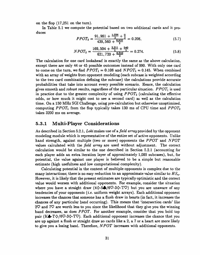
on the flop (17,251 on the tuni). In Table 5.1 we compute the potential based on two additional cards and it p r e

duces

The cdculation for one card lookahead is exactly the same as the above calculation. except there are only 44 or 45 possible outcornes instead of 990. With only one card to corne on the turn, we find PPOTr = 0.108 and NPOT* = 0.145. Wben combined with an array of weights from opponent modeling (each subcase is weighted according to the two card combinat ion defining the subcase) the calculat ions provide accurate probabilities t hat take into account every possible scenario. Hence, the calculat ion gives smooth and robust results, regardless of the particular situation. PPOTi is used in practice due to the greater complexity of using P POT2 (calculating the effective odds, or how much it might cost to see a second card) as well as the calculation time. On a 150 MHz SGI Challenge, using pre-calculation but otherwise unoptimized, computing PPOTl from the flop typicdly takes 130 ms of CPU time and PPOT* takes 3200 ms on average.

5.3.1 Multi-Player Considerations As described in Section 5.2.1, Loki makes use of a field array provided by the opponent modeling module which is representative of the entire set of active opponents. Unlike hand strength, against multiple (two or more) opponents the PPOT and NPOT values calculated with the field array are used without adjustment. The correct calculation would be similar to the one described in Section 5.2.1 (accounting for each player adds an extra iteration layer of approximately 1,000 subcases), but, for potential, the value against one player is believed to be a simple but reasonable est imate (high usefdness and low compu tational complexi ty ).

Calculating potential in the context of multiple opponents is complex due to the many interactions; there is no easy reduction to an approximate value similar to H&. However, it is likely that the present estimates are typically optirnistic and the correct value would worsen wi t h addi tional opponents. For example, consider the situation where you have a straight draw (40-54160-30-TO) but you are unaware of any tendencies of your opponents ( i. e. uniform weight arrays). Each additiond opponent increases the chances that someone has a flush draw in hearts (in fact, i t increases the chances of any pa r t i cda hand occurring). This means that 'intersection cards' like 2C) and 70 are worth less to you since the likelihood that they give you the winning hand decreases, as does PPOT. For another exarnple, consider that you hold top pair (K)T0/60-30-TV). Each additional opponent increases the chance that you are up against a flush or straight draw so cards like a 2, a 7 or a heart are more likely to give you a losing hand. Therefore, N POT increases with additiond opponents.

But over-optimism is not always the case; multiple opponents can improve your chances. For exampie, if you have a straight draw with small cards (40-5+/6&30- KO) and your opponents are likely holding high cards, then each additional opponent increases the chance that the upcoming card is not high. This will overall both decrease NPOT and increase P POT, although additional players also increases the size of the pot, which increases the value of Our draw.

These are only rough examples intended to dernonstrate the cornplex interactions involved in mult i-player considerations for hand potentid. The actual effect of each additional opponent is dependent on the probability distribution of possible hands and its relationship to the probability distributions of the other players, a s well as its relationship to your needed cards.

5.4 Summary

This chapter describes the methods used for evaluating our band in any particular situation. The algorithms presented are intended to provide good estimates of your winning chances.

For the pre-flop, we used an unsophisticated simulation technique for the calculation of pre-flop income rates. We feel that these values are suscient (will not be the limiting factor to the strength of the program), although there is room for improvement .

This chapter also describes the enurneration techniques used for evaluating hands (both strength and potential) after the flop. The algorithms, particularly in multi- player scenarios, abandon the treatment of some complexities in favor of simplicity and computation time. We have not invested the time to fully explore the magnitude of this error, however we believe it is minor in cornparison to the savings in time and cornplexit y.

Chapter 6

Betting Strategy

Using the game state, opponent models and hand evaluation derived from that data, the betting strategy determines whether to fold, cail/check, or betfraise. But exactly what information is useful and how should it be used? The answer to these questions are not trivial and this is one of the reasons that poker is a good testbed for artifi- c id intelligence. One approach would be to use the game theoretic optimal betting strategy, but, despite the fact that it is very complex to calculate, human opponents do not play optimally so this may not be the best decision in practice (leading to the most profit).

A minimal system could simply be based on hand strength ( i - e . ignore hand potential and simply betlcall based on the immediate strength of our hand). Refinements to the betting strategy would involve the addition of high-Ievel strategy concepts (like slowplaying or b lu5g ) . For each decision to be made, one of several miables (like PPOT) is compared to some threshold (which rnay be based on another variable, like pot s d d s ) . This structure uses expert knowledge but is easy to implement and the overhead is insignificant. All of these refinements are intended to be quick ways to select the play which (hopefully) has the largest expected value (EV), since cornputing the exact E V is not feasible. There is a real-time constraint, in that a single game of poker only takes a few minutes to play, and from Figure 4.2 we see that the game tree can be very large.

This chapter first describes the pre-flop betting strategy (which is treated as a special case). This is followed by an explanation of a simple post-flop (flop, turn and river) betting strategy (using only hand strength) which serves as a template, and then the rneasures and strategies that Loki uses for the post-$op rounds. Finally, unimplemented strategies are discussed.

Note that this chapter is included for completeness. The betting strategy is (so far, necessarily) ad hoc and therefore left undeveloped (it is a target for future im- provernent with computer-oriented techniques such as Monte Car10 simulation).

6.1 Pre-Flop Betting Strategy

The implemented preflop betting strategy is preliminary and makes use of expert information. It is sophisticated enough to not hamper overall performance so t hat the focus can be put on post-flop play (the more interesting portion of the game). L o k examines several variables, uses the expert knowledge to determine t hresholds for various betting actions, and chooses a strategy:

O MakeO: fold if it costs more than zero t o continue playing, otherwise check.

O Calll: fold if it costs two or more bets to continue (and we have not already voluntarily put money in the pot this round), otherwise check/call.

O Makel: like Cal11 except bet if there has not been a bet this round (with the big blind this cannot happen in the pre-fiop).

0 Cal12: always call/check (despite what the narne of this strategy suggests, even more than 2 bets).

Make2: betlraise if less than two bet/raises have been made this round, 0th- erwise c d .

a Make4: betfraise until the betting is capped, otherwise cdl.

Except for the small blind, which is given special treatment, Cal11 and Cd12 are effectively not used, so there are really only 4 different strategies. Once a strategy is selected it is fixed for d l subsequent actions in the pre-flop. The small blind is a special case due to only having to cal1 one half of a bet (so Callï is really Ca110.5 and Cd12 is really Cal11.5), and has fixed thresholds for these two strategies.

Cal11 (and hence Makel) has a special case folding requirement, that "we have not already voluntarily put money in the pot this round." This is a feature added after testing with human opponents on IRC. Many players were very agressive and would raise frequently. This meant that often when Loki called the blind with a decent hand (but not Cal12 or better), two or more players would then raise. causing Loki to fold. Due to this commonly exploited weakness, the kludge is necessary until some amount of opponent of modeling is implemented into the pre-flop.

The thresholds for selecting a betting strategy are determined from a set of linear formulas of the form

threshold(strategy) = base + inmement * position (6-1

where strategy is the betting strategy (e-g. M a k e l ) , base and increment are defhed by a human expert (see Appendix B), and position is the nurnber of players to act before it is the small blind's tum again (so, if numinpot is the number of players still in the pot, the srnall blind is position numinpot - 1, the big blind is position numinpot - 2, the first player to act is position numinpot - 3 and so on, until the button (dealer) who is position O).

For example, if Loki is playing tight against 3-4 players, the [base, incnmenf] values used for Make2 are [200,50] (based on Table B.1) so the formula used is

threshold(Make2) = 200 + 50 * position

based on Equation 6.1. That is, the coefficients used for the linear formula depend on both the vaxiable (group) and the parameter (tightness).

The variable group is based on the expected number of players (E-nurn_pla yers). which is

Enumglaye r s = num-guaranteed + (6.2)

probabilityglay r (numinpot - num-guaranteed).

There are three cases of interest for the expected nurnber of players. We round Enumglaye r s to the nearest integer and determine the appropriate group based on what range that value falls in: '2 players", '3-4 playersn and "5 or more players" (see Appendix B). The state variable numguaranteed is the number of players who have already put money in the pot (and have presumably committed to playing). This includes the blinds as well as ourselves (we assume we will play). Probabilityqlay is an expert-defined value for the average playing percentage of players (by default 0.60). Appropriate opponent modeling would provide much better estimates for this value, based on the observation of the current session .

The parameter tightness is a setting which affects the percentage of hands that Loki d l play (indirectly, by selecting a different set of thresholds). The t hree settings are tight, moderate, and loose (the default). With ten players these roughly translate into playing 18%, 21% and 24% of d l hands (the distinction is not large so the terms are a misnomer - al1 levels are relatively conservative).

There is one [base, inmement] pair per set of group, strategy and tightness values (Table B.l) so there are 27 pain total (since MakeO is the default strategy only three threshoids are needed for determining the strategy). Once the thresholds are determined, the actual strategy selected is dependent on the pre-calculated income rate (1 R) of the hole cards. Figure 6.1 describes the algorithm for select ing a strategy.

For example, consider a six player garne. We hold AO-TO and are playing tight- The first two players put in blinds, the next two fold, and it is Loki's tum. There is still one player, the button, who has not yet acted. So position = 1, numinpot = 4 and mm-guaranteed = 3 (including Loki). We then calculate

and use this to deterrnine group = 3 - 4 players". Then, using Table B.1 we calculate

threshold(Make1) = 50 + 50 * 1 = 100,

threshold(Make2) = 200 + 50 * 1 = 250, and threshold(Make4) = 580 + O + 1 = 580.

Finally, we h d the value of Our hand is I R = 491 and select the appropriate strategy. Since 250 1 491 < 580, we select the Make2 strategy, and raise.

/* Called t h e f irst t h e * t h e se lec ted s t r a t egy

FLOAT Enunq laye r s INTEGER group EOAT IR FLOAT t h r e s h n

/* detenaine t h e group

ue are asked f o r an ac t ion i n t he pre-flop, d i c t a t e s t he current and subsequent ac t ions */ myhand. STATE s t a t e , PARAlIETERS param)

/* axpected number of players */ /* n o , THREEORFOUR, o r FIVEPLUS */ /* incorne rate */ /* indexed by s t r a t e g i e s */

E s q l a y e r s = s t a t e .n-aranteed + param-probabi l i typlay * ( s t a t e .numinpot - s t a t e .num@aranteed)

if (s ta te-numinpot < 2.5) group = Tu0

e l s e i f (Esumqlayers >= 4.5) group = FIVEPLUS

e l s e group = THRLEORFOUR

/* ca lcu la te IR (see Appendix A ) and thresholds . */ IR = IR-table k r o u p ,myhand] /* only t h e s m a l l blind has d i f f e r en t thresholds f o r CALLl and C U L 2 */ th resh = SetThresholds (group .param. t igh tnass , state. position)

/* now use I R to se lec t t h e appropriate s t r a t egy */ if (iR>=threshCHAKE41)

s t r a t egy = -4 e l s e i f ( I R > s t h r e s h C W a )

s t r a t egy = M E 2 e l s e if (IR>--t;hresh [CU21 )

s t r a t egy = C U 2 e l s e i f ( I R > - - t h r e s h [ ~ l ] 1

s t r a t egy = ltAKE1 else i f (I~>=tbresh [CALLi] )

s t r a t egy = C U 1 e l s e

s t r a t egy = -0 re tusn s t r a t e g y

1

Figure 6.1: Pre-Flop Betting Strategy

6.2 Basic Post-Flop Betting Strategy

A minimal system for betting or calling could be based solely on the immediate strength of our haad. In fact, a more useful betting strategy could still use this basic system as a template and simply proceed to a hierarchy of alternative branches whenever the current decision is rejected. For example, if the initiai betting decision based on hand strength decides to fold we could fidl back on another consideration such as semi-bluffing. If we then do not decide to semi-bluff, we fa11 back on to another decision Iike pot odds. Each time the proposed action is rejected the next decision point c m be checked against some defined order of priority. Priority is dependent on how agressive the action is. Pot odds and showdown odds (described below) are Iow priority because they are passive cdinglchecking decisions (if we always used the pot odds decision first, we would never bet ). However, a strategy like check-raising is only used with a very strong hand so it would be given the highest priority ( L e . considered first ) .

A simple betting strategy, based on hand strength, is described in Figure 6.2. It uses a function c&ed Make which is used to show a level of strength appropriate for the hand held. The Make function is used in the pre-flop betting strategy and to sorne extent in the actual post-flop betting strategy.

6.3 Effective Hand Strength

The majority of betting decisions are made based on a variable which represents the strength of Lokt's hand in the current situation. Basic hand strength (HS,) is the probability that it presently has the strongest hand. This alone is not fully adequate when there are more cards to corne which can easily change the situation. For this reason, we compute the potentials PPOT and NPOT, which tell us Loki's probability of winningflosing given that it is currently behindfahead. Using these d u e s we can compute an estimate of Loki's chances of winning at the showdown (or of being the strongest after the next card, if it is the 00p and we are using PPOTJ. LVe define effective hand strength as

EHS = HSn + (1 - HSn) * PPOT - HSn * NPOT. (6.3)

Observe that on the river E HS = HSn7 since there are no more cards to be dealt. However, there are some problems with including N POT in the calculation. First ,

when we bet we do not know if Our opponent will play. Second, in many situations where we compute a high NPOT, it is often a better strategy to bet/raise to force the opponent out of the hand. So when effective hand strength is used as a betting decision (as opposed to a calling decision) it is preferable to use a more optimistic version, EH S' :

EHS' = HS, + (1 - HS,) * PPOT. (6-4)

This is on estimate which means "the probability that we are currently leading. or that we will improve to the best hand by the showdown."

/* BET/FUISE: when bets-toaake < nnmhets otherwise CEECK/CAU/FOLD appropria te ly */

H&e(INT bets-tosiake , STATE s t a t e )

/* bets-tomaice is the l eve l of s t reng th we oant t o show * namhtts is the number of be t s o r raises made by al1 players t h i s round * b e t s p t i n is the number we have vo lun ta r i ly put i n t h i s round * bets-to-cal1 is the number of be t s w e have yet t o c a l l */

i f (state-narabets < b e t s - t o ~ a k e ) re tu rn BETIRAISE

/* V e ail1 c a l l nnything if * - we have voluntarily put money in t h e pot t h i s round (see Section 6.1) * - betsfosiake >= 2 */

e l s e i f ( s t a t e - b s t s q u t i n > O 1 1 bets-toaiake >= 2 1 1 s t a t e . bets~ozall<=bets,toaialte)

re turn CEiECK/CALL e l s e

re turn FOLD

1

GetAct ion(FL0AT HSn, STATE state , P W T E R S param) 1

if (HSn >= param.make2) re turn Halce(2, s t a t e )

e l s e i f (HSn >= param.make1) re turn Hake(1 , s ta te )

e l s e re tu rn Malce(0, s t a t e )

1

Figure 6.2: Simple Betting Strategy

The basic betting decision used in Loki is similar to Figure 6.2, with the exception that EHS' is used instead of HS.. A Make2 hand is defined as a hand with E HS' 2 0.85. We raise when l e s t han 2 bets have been made this round, otherwise we call. A Makel hand is defined as a hand with EHS' 2 0.50. W e bet if no one else has, and c d otherwise, except when it is 2 bets to c d and we have not already called a bet this round. Finally, with E HS' < 0.50 we consider the strategies of semi-bluffing, pot odds and showdown odds (instead of resorting to MakeO as in Figure 6.2). These thresholds are an ad hoc but reasonable way to decide when to bet based on strength.

The Iack of the ability to raise beyond two bets after the 0op is a historical artifact, although not likely to be very limiting- Of course it must be addressed eventudy, but it is a low priority function and hopefully will be superseded by a more general betting strategy.

6.4 Semi-Bluffing The decision to semi-bluff has the next highest priority (meaning if we do not bet or call based on EHS' we consider semi-blufig). If we axe faced with O bets and have a high enough potential to call both a bet and a raise. we will open the betting ourselves. If none of the other players bet or raise we will continue to bet in subsequent rounds even wit hout sufficient potent ial (continuing to represent a strong hand while t here is a reasonable chance of winning the pot imrnediately). Semi-bluffing is used when PPOT >= Pot-Odds2, where

2 * b e t s i z e Pot-Odds2 =

(po t s i r e + 4 * b e t s i z e ) + 2 * b e t i i i z e -

The term '2 * be t s i z e ' represents the bet and raise we are saying we can call. The term '4 * betsize' represents the money the bettor and raiser will be putting in to the pot to match ours (2 bets each, including the assumption that the initial bettor would cal1 the raise). Since it is not possible to know how much is going to go into the pot, we do this as an approximation of the pot odds we would be getting.

Blufïmg in this manner has a positive side effect by contributing to deception. If Loki never bluffed the human opposition would recognize this after a few shorvdowns aad would quickly adapt, folding when faced with a bet or raise (lowering winnings). In fact, since Loki bluffs infrequently, the more experienced players on IRC often detect and exploit this predictable pattern.

6.5 Calling With Pot Odds

Pot odds is an important concept that difierentiates poker from many other games, and contributes to its usefulness as a testbed for concepts in the red world. Pot odds is the cornparison of your winning chances to the expected return from the pot. For example, if there is only a 20% chance that Loki has the best hand on the river. should we fold, call or bet? Assume the pot contains $20 after the only opponent bets $4. Calling in this situation will lose 4 times out of 5, at a cost of $4 each time. However, we win 1 time out of 5 for a profit of $20. Therefore, under these assumptions, a call is better than a fold, resulting in an average profit of 80.80 per hand. However, if the pot only contained $12, we shouId fold, since c d i n g would yield an average loss of $0.80 per hand.

On the flop and turn the calling decision is based on a slightly different concept. If PPOT = 0.20 then there is a 20% chance that the next card will give Loki a very strong hand. It does not necessarily win the hand, but for the sake of pot odds, we consider this to be the chance that Loki will clinch the hand with the next card (the current pot is Our winnings). This is a basic decision and does not take into account other nuances such as the fact that the other 80% of the time Loki may still have a reasonable chance of winning.

To make this calling decision we verify that the pot odds justify paying to receive one more card (or to play the showdown when we are on the river). We call when

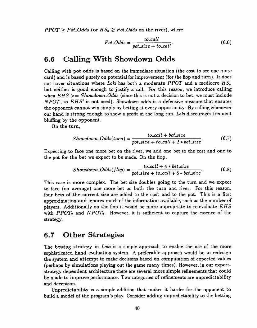
PPOT 2 Pot-Odds (or H S , 2 Pot-Odds on the river), where

t O-cal1 Pot-Odds =

p o t s i z e + to-cal['

6.6 Calling With Showdown Odds

Calling with pot odds is based on the immediate situation (the cost to see one more card) and is based purely on potential for improvement (for the flop and tum). It does not cover situations where Loki has both a moderate PPOT and a mediocre H S , but neither is good enough to justify a call. For this reason, we introduce calling when EHS >= Showdown-Odds (since this is not a decision to bet, we must include NPOT, so EHS' is not used). Showdown odds is a defensive measure that ensures the opponent cannot win simply by betting at every opportunity. By calling whenever our hand is strong enough to show a profit in the long run, L o k discourages frequent blufhg by the opponent .

On the turn,

to,cail+ b e t s i r e Showdaun-Odds(turn) = (6.7)

p o t s i z e +to-call+ 2 * b e t s i ; e '

Expecting to face one more bet on the river, we add one bet to the cost and one to the pot for the bet we expect to be made. On the flop,

to-cal[+ 4 * b e t s i z e Showdown-Odds( f top) =

p o t s i r e + to-call + 8 * b e t s i r e - (6 .8)

This case is more complex. The bet size doubles going to the tum and we expect to face (on average) one more bet on both the turn and river. For this reason. four bets of the current size are added to the cost and to the pot. This is a first approximation and ignores much of the information available, such as the number of players. Additionally on the flop it would be more appropriate to re-evaluate E HS with PPOTz and NPOT2. However, it is sufficient to capture the essence of the strategy.

6.7 Other Strategies

The betting strategy in Lo& is a simple approach to enable the use of the more sophisticated hand evaluation system. A preferable approach would be to redesign the system and attempt to make decisions based on computation of expected values (perhaps by simulations playing out the garne mâny times). However, in Our expert- strategy dependent architecture there are several more simple refinements that could be made to improve performance. Two categories of refinements are unpredictability and deception.

Unpredictability is a simple addition that makes it harder for the opponent to build a mode1 of the program's play. Consider adding unpredictability to the betting

based on an EHS' decision: we could use a linear scale so that we bet 50% of the time with a 0.50 hand, O% of the time with a 0.40 hand and 100% of the time with 0.60 hand.

Deception includes strategies such as pure blufEing, slowplaying and check-raising. It causes the opponent to make wrong assumptions about the current state of the game. Deception can also be used to make a play that does not necessarily lead to the highest expected value for the current garne but rather is intended as "fdse advertisingn to indirectly lead to increased profits in future hands. To be complete, al1 possible actions that one can witness from Loki should have a dual interpretation so no conciusions can be made with certainty. For example, in the present system ( wit hout check-raising) , if Loki checks, a knowledgeable observer can infer t hat Loki has a hand with EHS' < 0.5.

We have included some of these deceptive strategies successfully in later versions: check-raising, pure bl&g (betting with a weak hand on the river) and bdancing raises (sometimes raising instead of calling). They are currently used unpredictably (randomly). We also occasionally check-raise with a mediocre hand, so Our opponents cannot infer that we always hold a strong hand when we check-raise.

6.8 Summary

The full betting strategy algorithm is presented in Figure 6.3. It is an incomplete expert system using the objective hand evaluation techniques for the betting decisions, used for its easy implementation and low cost. This version has not been adjusted to use the opponent modeiing system, which was added afterwards. A more cornputer- oriented approach would be preferabie (for example, computing expected values by playing out several simulations) but the present system is sufficient to not significantly harnper the performance, and to allow for the easy introduction and testing of other high-level bet ting strategies (like semi-bluffing) .

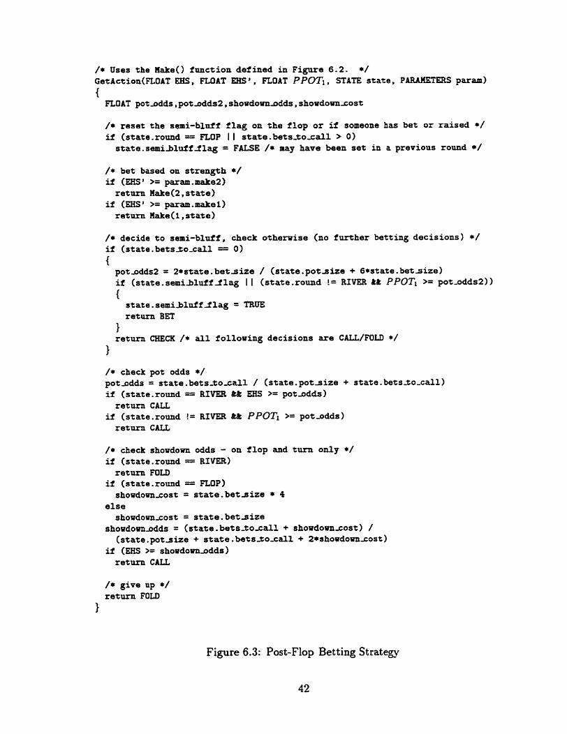
/* Uses the !Sake() frinction defined in Fignre 6.2. */ GetAction(FL0AT MS , FLOAT EHS ' , FLOAT P POTl, STATE s t a t e , P A F W E E R s param) {

FLOAT potsdds , p o t ~ d d s 2 , shoadorm~dds , showdovnçost

/* rese t the semi-blnff f l a g on t he f l o p or if someone has bet o r ra i sed */ if (state.ronnd = FLOP 1

s t a t e . semi4luff l l a g =

/* bet based on s t rength if (EHS >= param. malte21

re ta rn Halre(2, s t a t e ) i f (MS >= param.make1) return Hake(1,state)

/* decide t o semi-bluff, if ( s ta te . betsito-cal1 = {

1 s t a t e . b e t s - t o s a l l > 0 ) F U S E /* may have been s e t in a previous round */

check otheruise (no fu r the r bett ing decis ions) */ 0 )

potsdds2 = 2*state. b e t s i z e / ( s t a t e . p o t s i z e + ô*state .bets ize) i f (state.semibluff d l a g I 1 ( s t a t e .round != RIVER && PPOTl >= pot-odds2))

{ s t a t e . s emib lu f f f l a g = TRUE return BET

1 re turn CHECK /* al1 fo l lou ing decisions a r e CAU/FOLD */

1 /* check pot odds */ potsdds = s t a t e . be t s - t oza l l / ( s ta te . p o t s i z e + s t a t e . b e t s ~ o - c a l ) i f (state.round = RIVER && EfIS >= potadds)

re turn C A U if (state.round != RIVER && PPOTi >= p o t ~ d d s )

re turn CAU

/* check shoudown odds - on f l o p and tu rn only */ i f (state.round = RIVER)

re ta rn FOLD i f (state.round == FLOP)

showdounzost = state. b e t s i z e * 4 e l s e

showdounsost = state . b e t s i z e showdovasdds = ( s t a t e . b e t s - t o x a l l + shoudoanzost ) /

( s t a t e . p o t s i z e + state. bets2o-cal1 + 2*shoudownrost) if (EHS >= shoodownadds)

re turn CALL

/* give up */ r e t a rn FOLD

1

Figure 6.3: Post-Flop Betting Strategy

42

Chapter 7

Opponent Modeling

Ln strategic games like chess, it is acceptable to assume that the opponent is perfect because that assumption does not result in a significant loss in performance for the algorithm against weaker players. Opponent modeling has been attempted in tw* player games as a generalization of min ima but with limited success [5] [9]. In contrast, not only does opponent modeling have trernendous value in poker, it can be the primary distinguishing feature between players at different ski11 levels. If a set of players al1 have a comparable knowledge of poker fundarnentals, the ability to alter decisions based on an accurate model of the opponent may have a greater impact on success than any other strategic principle.

Having argued that some form of opponent rnodeling is indispensable, the actual method of gathering information and using it for betting decisions is a complex and interesting problem. Not only is it difficult to make appropriate inferences from certain observations and then apply them in practice, it is not even clear how statistics should be collected or categorized.

This chapter describes opponent modeling in Loki. Using the betting history of the opponents, it determines a likely probability distribution for their hidden cards which is used by the hand evaluation system. A minimal system might use a single fixed model for all opponents in a given hand, based on the cards played to the flop by typical players. The system in place in Loki generates a model for each opponent and maintains information between games. It is a simplistic first approximation t hat takes specific observed information and transforms it to a more useful form. However, this is sufficient to demonstrate a significant performance improvement using only a simple analysis of context.

The first section discusses the representation of the model: the action frequencies for seIect decision categories and the weight array for d l the possible two card holdings. The second section explains the learning system (how the weight array is determined and how the action frequencies are used for this). The final section discusses how the weight array is used in hand evaluation, in particular how the field array is calculated.

7.1 Representation

There are two structures that comprise an opponent model, the weight array and the action frequencies, and both are updated by the learning portion of the opponent modeling system. The weight array is actudly a model of the opponent's hand: it is reset at the beginning of each hand and contains information pertaining to what cards the opponent may be holding. It is used by the hand evaluation system to give more accurate estimates of hand strength. The action frequencies are inter-game statistics on how many times the opponent bas taken each action in a given situation. They are used by the learning system to appropriately update the weight array, and they could be used by the betting strategy systern.

7.1.1 Weight Array

The weight array is a mode1 of the opponent's hand. Each opponent p has an array of weights w,[h] where h represents each possible two card hand. There is a weight associated with each h (reset to 1 each new hand) which approximately represents the conditional probability that player p would have played in the observed manner (given that they held hand h). We cal1 these values weights because they act as multipliers in the enurneration computations. If we want a probability distribution of possible hands held by p, we normalize the array by dividing each entry by the total sum of a11 the entries (the number of vdid entries depends on which hands are still possible). The nomalized entries w i [hl represent the conditional probability that player p holds hand h (given the betting history).

This is a very detailed representation, although there is some error since interdependencies are not considered. In the multi-player scenario we do not address the fact that different opponents cannot hold the same card. For example, if we assign a high relative probability to one specific opponent holding an Ace, we do not reduce the relative probabilities of the other opponents holding an 4ce. This also means that when a player folds, the information regarding which hands that player may have held is discarded. The weight array is not adjusted with respect to the weight arrays of the other opponents. However, we feel this error is minor in cornparison to the savings in complexity and computation time.

7.1.2 Action Fkequencies

When ân opponent's action is used to adjust their weight array, it is important to take into account what type of opponent it is. As a first approximation we can assume all opponents play the same (e.g. raise with the top 15% of hands, and so on). In this case, all that matters when adjusting the weight array is the action taken, and not the type of player. This is called genen'c opponent modeling because the re- weighting systern is identical for each player. However, initial tests against human opponents revealed that this was an incorrect assumption. A loose and aggressive opponent might bet with almost anything and therefore a bet should not be taken

too seriously. On the other hand, a tight and passive opponent will usually only bet with a very good hand.

To account for this we introduce specific opponent modeling. Statistics for each opponent are tabulated and used to c d d a t e betting frequencies, and these frequencies adjust how the re-weighting systern works. For example, if we observe that a certain opponent bets 80% of the time when acting h s t on the flop, then we will take this into account when adjusting the weight array for a bet observed by that opponent in t hat same situation.

This introduces a new problem. Statistics can be retained for a large number of categories. Consider, for example, that we index each frequency by the nurnber of active opponents (1, 2, 3+; 3+ is the '3 or more7 category), total raises this round (0, 1, 2+), bets to cal1 (O, 1,2+), and game round (pre-flop, flop, turn or river). The 'ta+' classification is useful for putting together similar cases. In this examplet each situation fits into one of 3 * 3 * 3 * 4 = 108 categories. It would take a large number of observed games before we had sficient data for some categories. In fact, this categorizatioo could easily be made more complex by dso tkking into account other important Mnables such as table position, remaining cdlers, and previous action taken (to catch advanced strategies Like check-raising).

The finer the granularity of the data collected, the harder it is to get meaningful information (more observations are required). There are two ways to make it more manageable. The first way is to distinguish many different categories for the data collection phase (a fine level of granularity) and then combine classes that have similar contexts in the data usage phase. The other, less sophisticated, approach is to simply have few different categories for the data collection phase. This dlows the frequency calculations of the data usage phase to be quick and simple. This is what we have done.

Data is categorized into 12 categories, indexed by (O, 1, 2+) bets to call and the 4 different game rounds. This is a simple first approximation but is sufficient to determine if this level of opponent modeling can be beneficial. It also has the advantage of enabling the program to learn 'quickly', although less accurately. It is easy to adjust the definition of the context for the purpose of gathering statistics. The learning system (the re-weighting system that uses this information) is only interested in the frequency of an observed action and not how that figure was calculated.

For each opponent p, we determine the category c of the obsewed action (the con- tezt - amount to call and game round) and record the action a taken (fold, check/call, bet /raise) by incrernenting Tp[c] [a]. When we need to know the frequency t hat a player has taken a certain action in a certain situation, f,[c][a], we simply compute the ratio of Tp[c] [a] versus Sp[c] (the t o td number of actions recorded for that context):

Default Frequencies

Until enough data has been accumulated for a category (30 points, this value was selected arbitrarily), we weight the frequencies with hard-coded defaults' d[c][a], and mix the observed frequencies with the defaults, using linear interpolation:

20 S c fp[c][a] * + d[c][a] * when S,[c] < 20;

(7-3) f~ [CI [al otherwise.

However, each player will play the eulier rounds more than the Iater rounds ( i - e . more pre-flops than flops, and so on). Assuming that a player's style does not change drastically between rounds, we can take advantage of data gathered in prior rounds and use only one set of defaults and a recursive definition of frequency. To this end, we must first adjust the notation to consider the round. Given that the definition for the category c is composed of a round r and number of bets to cal1 6, we can dso define c as (r , b) where r = O for the pre-flop. Now we can recursively define the new frequency function f" based on the reduced set of defaults d' [b] [a]:

An alternative approach would have b e n to use Loki's own frequencies as the default behavior for opponents, however the majority of human players on IRC were observed to play much looser than Loki. The default frequencies were therefore based on a typical IRC player (and do not involve any additional computation).

7.2 Learning

Each time an opponent makes a betting action, the weights for that opponent are modified to account for the action. For example, a raise increases the weights for the stronger hands likely to be held by the opponent given the flop ctlrds, and decreases the weights for the weaker hands.

With this re-weighting system we consider two distinct levels of modeling, as discussed in Section 7.1.2. First, an opponent's betting actions are used to adjust the weights. The actual transformation function used for the re-weighting is independent of the player in question. A different weight array is still maintained for each opponent, but a raise observed in a certain category is treated the same for al1 players. Second, we maintain data between games (the action frequencies) and

'See Appendix B for the values used.

these frequencies are used to adjust the transformation function itself. This technique is called specific opponent modeling, because the re-weighting depends on the opponent 's model. In fact, the only difference between the two levels is that wi thout specific opponent modeling, the re-weighting function always uses the generic defaul t frequencies ( i. e. f:[r, b] [a] = d[b] [a]).

The remainder of this section discusses the general idea of the re-weighting system. and then presents the specific details with respect to the pre-tlop and post-flop rounds.

7.2.1 Re-Weighting System

The weight adjustment for any particular subcase is based on the threshold hand value needed for the observed action. The threshold is in turn based on the observed frequency of folding, calling and raising of the player in question (or the default frequencies when we are using generic opponent modeling or have insufficient data). From these frequencies we deduce the average (p , representing the mean hand) and spread (a, to account for uncertainty) of the threshold needed for the observed action.

The values p and o define an expected distribution of hands to be played, realizing a transformation function for re-weighting. We take some ranked distribution of al1 possible hands hel i ( I R for the pre-flop and E HS' for the post-flop rounds, meaning we presume Our opponents rank hands like we do) and each hand h is compared to p and o and re-weighted accordingly (see Figures 7.1 and 7.2). When the value for h is equal to p, the re-weighting value is 0.5; when it is more than a below p, it is 0.01; when it is more than a above p, it is 1 (the weight is unchanged); and when it is within O of p it is lineôrly interpolated between 0.01 and 1 (we use a simple linear interpolation because it is easy and we do not know what the distribution should look like). Since we do not want to completely d e out any legal subcase we do not allow the weight to go below 0.01.

The value p is based on the threshold needed for the observed action, which is in turn based on the frequency. For example, consider that player p has been observed 100 times in the pre-flop with 2 bets to c d : 20 times it was raised, 70 times called and 10 times folded. If we wanted to re-weight based on a raise we compute the

- 0.20, meaning the threshold is frequency of raising: F = f;[Q, 21 [mise] = - p = 1 - F = 0.80 (player p raises with the top 20% of hands). However, if we wanted to re-weight based on a c d (frequency 0.70) we must note that the threshold for a cal1 is not p = 1 - 0.70 = 0.30 but is rather 0.70 below the raise threshold: p = 0.80 - 0.70 = 0.10 (player p c d s with the middle 70% of hands). There are other intricacies dependent on the actual round of play, such as determining o and using I R values (which are non-percentile), which will be discussed in the following sections. One irnmediately noticeable source of error is that this system presumes a proper distribution over the hand rankings ( i . e. the hands above p = 0.80 represent 20% of d l hands). This is not true for the post-Bop rounds, because EHS' is optimistically increased with P POT. However, the relative ranking of hands is still correct.

As a final note, to prevent the weight array from being distorted by automatic or false actions, we only perform one re-weighting per model per round. We store a

constant l o s s t 0.01 constant high* 1.00

/* s e i g h t n 1s the weight anay from the beginning of the round */ Reweight (FLOAT p , FLOAT o. FLOAT ueight 0 )

FLOAT reaeight FLOAT handvaliie /* depending on the round t h i s is e i t h e r I R o r MSa */ CARDS hand for each subcase (hand)

handvalue = GetHandValae(hand) /* in te rpola te i n t h e range p f u */ reweight = (handvalue - F< + o) / (2*c ) if ( r ewe igh t~ lowf l ) reaeight = low-ut i f (reweight>highst ) reaeight = h i g h d weight band] = weight [ h a d j * reweight /* don*t l e t t he weight go belou 0.01 */ if (seight [hana clorrot) weight [hand] = l o w s t

1

Figure 7.1: Re-weight ing Function Code

Figure 7.2: Re-weighting Function

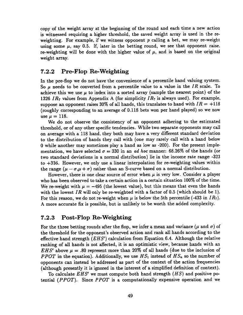
copy of the weight array at the beginning of the round and each time a new action is witnessed requiring a higher threshold, the saved weight array is used in the re- weighting. For example, if we witness opponent p calling a bet, we may re-weight using some p, Say 0.5. If, later in the betting round, we see that opponent raise. re-weighting wiU be done with the higher value of p, and is based on the original weight array.

7.2.2 Pre-Flop Re-Weighting

In the preflop we do not have the convenience of a percentile hand valuing system. So p needs to be converted from a percentile value to a value in the I R scale. To achieve this we use p to index into a sorted array (sample the nearest point) of the 1326 IR7 values from Appendix A (for sirnplicity IRï is always used). For example, suppose an opponent raises 30% of al1 hasds, this translates to hand with I R = +Il8 (roughly corresponding to an average of 0.118 bets won per hand played) so we now use p = 118.

We do not observe the consistency of an opponent adhering to the estimated threshold, or of any other specific tendencies. While two separate opponents may call on average with a 118 hand, they both may have a very different standard deviation to the distribution of hands they call with (one rnay rarely cal1 with a hand below O while another may sometimes play a hand as low as -200). For the present implementation, we have selected a = 330 in an ad hoc manner: 68.26% of the hands (or two standard deviations in a normal distribution) lie in the income rate range -323 to +33d. However, we only use a linear interpolation for re-weighting values within the range ( p - a y + o) rather than an Scurve based on a normal distribution.

However, there is one clear source of error when p is very low. Consider a player who has b e n observed to take a certain action in a certain situation 100% of the time. We re-weight with p = -493 (the lowest value), but this means that even the hands with the lowest I R will only be re-weighted with a factor of 0.5 (which should be 1). For this reason, we do not re-weight when p is below the 5th percentile (-433 in IR;). A more accurate fix is possible, but is unlikely to be worth the added cornplexity.

7.2.3 Post-Flop Re-Weighting

For the three betting rounds after the flop, we infer a mean and miance (p and a) of the threshold for the opponent's observed action and rank al1 hands according to the effective hand strength (E HS') calculation from Equation 6.4. Although the relative ranking of all hands is not afFected, it is an optimistic view, because hands with an E H S above p = .80 represent more than 20% of all hands (due to the inclusion of PPOT in the equation). Additionally, we use HSi instead of HS, so the number of opponents can instead be addressed as part of the context of the action frequencies (although presently it is ignored in the interest of a simplified definition of context).

To calculate E H S we must compute both hand strength (HS) and positive p e tential (PPOT) . Since PPOT is a computationally expensive operation and we

must obtain PPOT values for about 1,000 hands every cal1 to the re-weighting function, we use a cmde but fast estimating function (P POT,). In terms of cost, PPOT, << PPOTl << PPOT2. It is cmde because it ignores much of the available information (such as weight arrays) and looks for a few features about the hand, using heuristics to associate a value to each. For example. if the board has only 2 diamonds of our Ccard diamond flush draw, then we have 9 outs (1 out per remaining card). but if the board has 3 diamonds, each of the remaining cards is worth 0.5 to 1 out, depending on the rank of your suited hole card (a Two is worth 0.5 and an Ace is worth 1). This is because we are more likely to be up against other diarnond flush draws. PPOT, approximates very roughly our winning chances given each possible card to be dealt). This function produces d u e s within 5% of PPOTl, 95% of the time (this is from a random sampling of five card unweighted cases). Since these values are amortized over about 1,000 possible hands, the overall eflect of this approximation is small.

However, the opponent is also likely to play some hands based on the pot odds required for the action (i.e. the decision is not always based on EHS'). For this reason we have introduced an adjustment to the re-weighting algorithm for the post- flop. When PPOT, is sufficient to warrant calling the pot odds, which is

the weight for that subcase is not reduced. This is a simplification of the betting decision the opponent could be making based on the pot size, however we feel it is sufficient to capture enough cases to prevent hands with low EHS' but high potential from being severely under-estimated. The new re-weighting algorithm can be found in Figure 7.3.

What value do we use for o? We chose to use a typicai value of o = .2 at p = .5 (interpolating over the range .3 to .7) and to increase a with smaller p while decreasing it for larger p. This reflects the tendency for loose players (with low p ) to exhibit more uncertainty and tight players (with high p ) to adhere more consistently to the threshold. Hence, we use o = 0.4 * (1 - p ) .

However, as was the case with preflop re-weighting, there is a clear source of error when p is very low. Observe that the area of the re-weighting function is a rectangle of height 1 and width 1 - ( p + o), with a triangle between p - a and p + O (Figure 7.2). That is,

(if we were to ignore the area due to the minimum re-weighting factor of 0.01). But, since the function domain is bounded by O, when o > p ( p < 0.2857) we have A < 1 - p. For the weaker hands, the re-weighting factor is too low. When we are in this special case, we compensate by changing the re-weighting function so that at EHS' = O the re-weighting factor is T instead of 0.01 (and the function interpolates linearly between r and 1 when the hand value is between O and p + O ) .

The value r is calcdated to give A = 1 -p. The function now looks like a rectaagle to the right of p + c, a triangle of height 1 - r (width p + O ) and a second rectangle

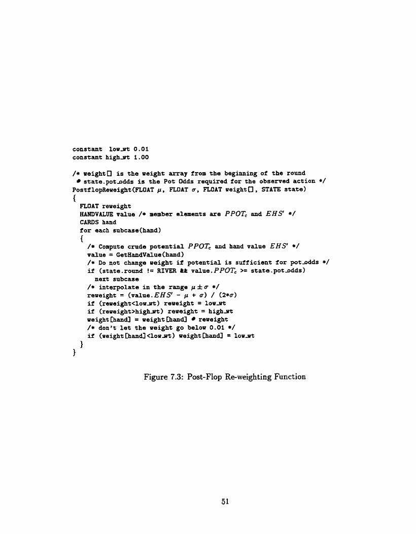
constant l o u s 0.01 constant h i g h s t 1.00

/* u e i g h t a is t h e weight array from t h e beginning of t h e round s t a t e - p o t a d d s is t h e Pot Odds required f o r the observed a c t i o n */

Postf 1opReweight (FLCIAT p. FLOAT u , FLOAT weight O , STATE state ) {

FLOAT reweight HANDVALUE value /* member elements are PPOT, and EHS' */ CARDS hand f o r each sabcase(hand) {

/* Compute crude p o t e n t i a l PPOT. and hand value EHS' */ value = GetHandValue (hand) /* Do not change weight if p o t e n t i a l is s u f f i c i e n t f o r p o t a d d s */ i f ( s t a t e .round != RIVER && value. P P OT, >= state . p o t s d d s )

next sabcase /* in te rpo la te i n t h e range p f u */ reueight = (value. EHS' - p + a ) / (2*u) i f ( reweight<loust ) reweight = l o u s t i f (reweight>higàirt) r eae igh t = highrFt weight [ h d = weight Chand reaeight /* don 't let t h e ue igh t go below 0 .O1 */ if (ueight ( h a 4 ~ 1 o u a - t ) s e i g h t [hand] = l o s d

1 1

Figure 7.3: Post-Flop Re-weighting Function

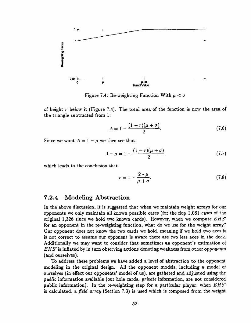
Figure 7.4: Re-weighting Function With p c cr

of height r below it (Figure the triangle subtracted from

Since we want A = 1 - C( we

7.4). The total area of the function is now the area of 1:

then see that

which leads to the conclusion that

7.2.4 Modeling Abstraction

In the above discussion, it is suggested that when we maintain weight arrays for Our opponents we only maintain d l known possible cases (for the flop 1,081 cases of the original 1,326 since we hold two known cards). However, when we compute EHS' for an opponent in the re-weighting function, what do we use for the weight array? Our opponent does not know the two cards we hold, meaning if we hold two aces it is not correct to assume our opponent is aware there are two less aces in the deck. Additionally we may want to consider that sometimes an opponent's estimation of E H S is i da t ed by in turn observing actions denoting weakness from other opponents (and ourselves) .

To address these problems we have added a level of abstraction to the opponent modehg in the original design. All the opponent models, including a model of ourselves (in effect our opponents' model of us), are gathered and adjusted using the public information amilable (our hole cards, private information, are not considered public information). In the re-weighting step for a particular player, when EHS' is calculated, a field a m y (Section 7.3) is used which is composed from the weight

arrays of d l the opponents of that player. As a result, the second re-weighting in a round is performed within the context of the f is t .

Of course, when we compute hand values for Our betting strategy, we use al1 available information and do not include all the subcases which use one or both of Our hole cards. Since the weight arrays have been normalized with these subcases included, some additional minor error is introduced.

7.3 Using the Mode1 At present, the action frequencies are only used in the re-weighting module (dthough this type of information could be useful in the betting strategy module). The only opponent information used externdy is the weight array, which is used in the hand evaluation module (Chapter 5). In that context, since each subcase has a specific weight, the array is used to calculate weighted sums and to infer better estimates of hand strength (which can be expressed as the total weight of al1 subcases that are weaker than you, added to half the total weight of ail tied subcases, divided by the t o t d weight of al1 subcases). Note that when used in this fashion the weight m a y does not need to be normalized.

7.3.1 The Field Array

In Chapter 5 we were presented with a problem: how to use the information available in multiple weight arrays to get a general value for strength and potential. The solution was the field array, an intuitive approach that fits into the existing frarnework. We average (or add, since in the relative sense they are the same operation) the weight anays of aIl the opponents to give a new array representing the entire table. However, since the weights represent relative probabilities, we must normalize the individual weight arrays (to the same scale) before they can be combined. Specifically, when we need to calculate hand values for player p, we calculate a field array that is the average of the normalized weight arrays of d l players except p.

This approach does introduce a srnall amount of error by abandoning some second- order considerations with respect to intersection cases, but again this error is minor when compared to the reduction in complexity. For example, if we want to compute the probability, given the appropriate normalized weight ôrrays, that either statement A (player 1 holds AI-AC)) or statement B (player 2 holds A ç A U ) is true we need to compute

P ( A or B ) = P ( A ) + P ( B ) - P ( A and B).

In fact, it is significantly more complex than this. For each subcase we would need to also d e out dl the other intersecting subcases (e-g. the probability that player I holds A&AP precludes player 2 holding either the A b or the AO).

7.4 Summary

The opponent modeling module includes a data accumulation system to infer action frequencies, and a mode1 of the player's hand represented by an array of weights. The action data gathered is based on a coarse definition of context , however i t is only intended as a simple framework to examine the feasibility of the approach. It is easy to adjust the definition of context because the learning system is only interested in the resulting frequency of an observed action, and not how that value was calculated. A lot of the potential data that could be accumulated is cunently ignored. For example. variance is not measured so a l l opponents are presently assumed to have the same level of uncertainty or consistency in their actions. We also do not consider recency (applying more weight to recent data points) although this is a more complex change to the present system.

There are two different Ievels of opponent modeling that can be examined. In generic opponent modeling the action frequencies are always assumed to be the same (predetermined defaults) and the only opponent nodeling that is done is by infer- ring the weight array (the re-weighting system). In specific opponent modeling, the observed action frequencies (specific to each opponent) are used to adjust the re- weighting system itself. The difference between the two systems can be exarnined in the function at the heart of the opponent rnodeling (Figure 7.5).

The re-weighting system is the complex portion of the opponent modeling system. It involves leaniing the distribution of probable hands held based on observed actions and storing this information in an array of weights (which are the relative probabilities that the opponent would have played that hand given the observed actions that game). The re-weighting system is given a certain p and o representing the threshold required for making the observed action, under whatever hand ranking measure is most appropriate: I R for the pre-flop and EHS' for the post-flop rounds. A linear interpolation transformation function (based on p and o) is applied to the weight array to give a new weight array. There are some problems with the system. For example, o is a fixed expert value when it should be based on observations. However, more importantly we never do inverse re-weightings ( L e . a call or check should suggest an upper threshold of hands the opponent likely does not have).

Of course, the opponent's decisions may in reâlity be based on a different rnetric than I R or EHS', resulting in an im~erfect model. There are other problems with the reweighting system, such as the presumption that the hand rankings are properly distributed (EHS' is an optimistic view). However, forming a perfect rnodel of the opponent is in general unboundedly difficult, since their exact actions are unknowable. New techniques can improve the results, but the current method does capture much of the information conveyed by the opponent's actions.

In cornpetitive poker, opponent modeling is more complex than portrayed here. One also wants to fool the opponent into constmcting a poor model. For example, a strong poker player may try to create the impression of being very conservative early in a session, only to exploit that image later when the opponents are using incorrect assumptions. In two-player games, the M' algorithm allows for recursive definitions

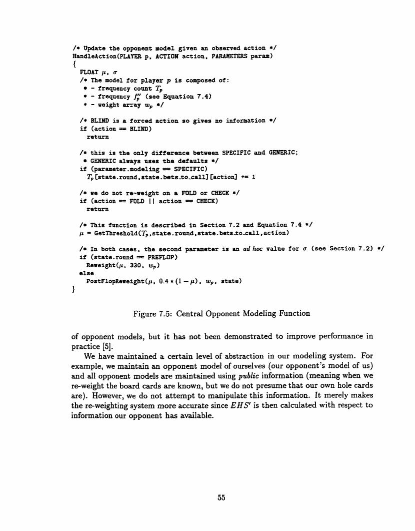
/* Update the opponent m o d e l given an observed a c t i o n */ HandleActîon(PLAYER p , ACTION a c t i o n , PAlWEERS p a r d

FLOAT p , a /* The model for play- p is composed of :

- freqnency count Tp * - fsequency f: (see Equation 7.4) * - ueight array wp */

/* BLIND is a forced a c t i o n so gives no information */ if (act ion = BLIND)

r e t u r n

/* t h i s is t h e o d y dïfference between SPECIFIC and GENERIC; GENERIC alaays uses t h e d e f a a l t s */

îf (parameter-modeling = SPECIFIC) Tpcstate.romd,state.bets-tosalll [ a c t i o d += 1

/* we do not re-weight on a FOU o r CHECK */ if (action = FOLD 1 I a c t i o n = CHECK) retarn

/* This f a c t i o n is desc r ibed in Section 7.2 and Equation 7.4 */ p = Getmeshold(TP ,state . round,s ta te . b e t s ~ o - c a l 1 , ac t ion)

/* In both cases, t h e second parameter is an ad hoc value f o r a ( see Section 7.2) */ if (state.rotmd = PREFLOP)

Reoeight ( p , 330, wp else

Pos tF ïop~eae igh t ( p , 0.4 * (1 - p ) , wp, s t a t e ) 1

Figure 7.5: Central Opponent Modeling Function

of opponent models, but it has not been demonstrated to improve performance in practice [5].

We have maintained a certain level of abstraction in Our modeling system. For example, we maintain an opponent model of ourselves (our opponent's model of us) and al1 opponent models are maintained using pubüc information (meaning when we re-weight the board cards are known, but we do not presume that our own hole cards are). However, we do not attempt to manipulate this information. It merely rnakes the re-weighting system more accurate since E HS' is then calculated with respect to information Our opponent has available.

Chapter 8

Experimentation provides a simple way to determine the effectiveness of changes, or to identify potential problems and shortcomings in the system. For Loki we have used a variety of different experimentd methods. The primary method is self-play simulation between different versions of the program. The other methods, much more difficult to interpret but presented as mecdotal evidence, involve play against other cornputer programs or human opponents through an on-line poker server running on IRC (Internet Relay Chat).

8.1 Self-Play Simulations

Self-play simulations offer a convenient method for the cornparison of two or more versions of the program. In addition to verifying that a certain enhancement has a beneficial effect, i t is possible to quantify the contribution made by each new component to the system. Since al1 participants in the simulated game are versions of the program, play can proceed at a rapid pace, and results can be based on large (statistically significant) sample sizes.

The self-play simulations use the duplicate tournament system descri bed in [2], based on the same principle as duplicate bridge. Since each hand can be played with no memory of the cards dealt in preceding hands, it is possible to replay the same deal, but with the participants holding a different set of hole cards each time. This system simulates a ten-player game. Each hand is replayed ten times (ten trials), shufaing the seating mangement so that every participant has the opportunity to play each set of hole cards once, and no two players are seated in the same relative position more than once (so, for instance, each player will play directiy behind each other player exactly once). The hole cards are always in the same betting order so those belonging to the srnd blind are identical in each trial. The seating permutations are listed in Table 8.1 (T = 10).

This arrangement greatly reduces the "luck elernent" of the game, since each player will have the same number of good and bad hands. The differences in the performance of players will therefore be based more strongly on the quality of the decisions made in each situation. This large reduction in natural variance means that

I 11 Seat Number for Each Player l / Round 1 2 3 4 5 6 7 8 9 T

Table 8.1 : Seat ing assignments for tournament play (reproduced from [2] )

meanîngfd results can be obtained with a much smaller nurnber cf trials than in a typical game set t ing.

There are numerous different ways to use self-play simulation to test different versions of the program. One simple application would be to play five copies of a new version against five copies of an older version, differing only in the addition of one new feature. If the new component has irnproved the program (against itself), then the newer version will win against the older version. The average rnargin of victory, in terms of expected number of small bets per hand, can also give a preliminary indication of the relative value of the new enhancement.

However, one must be carefd when drawing conclusions from self-play experiments. It is important to not over-interpret the results of one simulation [Il. With the above format, there are limitations to how much can be concluded from a single experiment, since it is representative of only one particular type of game and style of opponent. It is quite possible that the same feature will perform much worse (or much better) in a garne against human opposition, for example. A wider variety of testing is necessary to get an accurate assessrnent of the new feature, such as changing the context of the simulated garne.

However, most versions of Loki are very similar and have fairly conserntive styles. It is quite possible that the consequences of each change would be different against a field of opponents who employ difTerent piaying styles. For example, against several human playen, the effect of the weighting function may be much bigger than that of hand potential. Inter-dependencies between the involved players can dso affect results. The second-best player may perform fist overall if it can exploit a particular bad player more than the best player can.

8.2 Other Experiments

Loki has been tested for extended periods of time in more realistic settings against human opposition (and an occasional cornputer player). For this purpose, the program participates in an on-Line poker game, ninning on the Intemet Relay Chat

(irc.poker.net). Human players connect to IRC and participate in games conducted by dedicated server programs. Bankroll st atist ics on each ployer are maint ained. but no real money is at stake, and this may contribute to results being a little optirnistic. There are three different garnes amilable for limit Texas Hold'em. For the first level. you begin with $1000 and the betting scale is 10-20. Once you have $2000 ( i - e . won a net of $1000) you axe allowed to play in a second game where the betting scale is 2û-40. At $5000 you are allowed to play in a third game where the betting scale is 5û-100. The competition becornes much stronger at each level, but it is more difficult to find opponents, so games at the higher levels are less common. Early versions of Loki participated in games with 2 to 12 players. Later the server was changed to d o w only 2 to 10 players.

Play ing short-handed (2-4 players) emphasizes the need for strong opponent modeling. Typically, with many players (5 or more) the computer can win in the long run by playing the odds, usually because there are some bad players. With only a few opponents, we face many one on one situations where the non-mathematical elements of the game become more important. When those few players are strong (or colluding), Loki loses a large amount of money. It does not "give up" in a bad situation, so it continues to lose. Since games go by significantly faster, there is too much data in this limited context. We ignore results for garnes with 2 to 4 players because the overall results are distorted. AU the reported results are for games with 5 to 12 players (or 5 to 10 in the later sessions).

As this is not a closed environment, the natural variance in these games is very high, and the results depend strongly on which players happen to be playing. Con- sequently, not enough information has ben gathered to make any safe conclusions.

Very early versions of Loki had mixed results on the IRC server, but played too few garnes to be conclusive. However, it appeared to play a t about the same level as the average human puticipant in the open games. roughly breaking even over the course of about 12,000 hands. Opponent modeling appeared to be much stronger: in one session of 8,894 games (5 to 12 players), a version using generic opponent modeling (GOM) achieved a winning rate of 0.07 small bets per hand (this places Loki comfortably in the top 10% of players who play the 10-20 games on the server). In a later session of 29,301 games (5 to 10 players), another version that used specific opponent modeling (SOM) achieved a winning rate of 0.08 smalI bets per hand. While the difference between the two modeling versions may not be significant, they both win consistently and perform much better than the previous versions.

Recognizing that many human opponents were easily identifying when Loki had a strong or weak hand (occasional serni-blufhg did not add enough deception), we added some new deceptive strategies: pure bluffs (betting with the weakest hands on the river), balancing taises (occasiondly raising instead of calling), and check- raising (following a check with a raise in the sarne round). Check-raising is normally used with the strongest hands, but to ensure that no information can reliably be gained from any particdm action, we also use %ken check-raises with mediocre hands. However, these are simply more expert niles (e.g. check-raise 60% of the tirne with three callers behind us when E H S >= 0.92). We are interested in machine-

dependent approaches to computer poker ahere Loki can discover for itself what the best strategy is in a situation (which makes it easier to introduce opponent modeling into such decisions). So we are not interested in the performance contribution of any particular strategy. However, the introduction of these advanced tactics probably explains why the following results are better. The two opponent modeling versions that use these features are GOM' and SOM'.

We used these stronger features to see if we could find a noticeable performance difference between GO Mt and SU Mf. In 35,607 games, SOM' maintained a winning rate of 0.12 s m d bets per hand. In 36,299 games, GOM' maintained a winning rate of 0.10 s m d bets per hand. This is stronger evidence that specific opponent modeling is better. In fact, we believe that it may not be worth as much against the weaker class of human players (in the 10-20 game) and may lead to a stronger disparity in the higher level games.

In the stronger IRC game (20-40), earlier versions of the program without o p ponent modeling lost, averaging about -0.08 small bets per hand in 2,334 games. This is too s m d a sample size for conclusive results, but strongly suggests it was a losing player overall in these games. Opponent rnodeling demonstrated a noticeable difference at this level; SOM averaged about +0.05 small bets per hand in 34,799 games. This was probably iduenced by good results early on (before the human players had adjusted to the new style of Loki) so it is probably closer to a break-even player. However, this is noticeably better than the earlier version wit hout opponent modeling. We have have not tested GOM, GOMf or SOMf at this level.

A third form of competition was introduced strictly against ot ber computer p r e grams on the IRC server, called BotWarz. In BotWarz 1, four programs participated, using three copies of each in a 1Zplayer game. Two programs, ROOlbot and Loki, were clearly dominant over the other two, Xbot and Replicat, with the more es- tablished ROOlbot w i ~ i n g overdl. In 39,786 hands, Loki averaged about +0.03 smdl bets per hand. It should be noted, however, that this cornpetition is representative of only one type of game, where al1 the players are quite conservative. Replicat in particulax performed much better in the open games against human opposition than in this closed experiment, in which i t lost the most money. Also, despite the closed environment, the miance was still quite high.

There were also noticeable interdependencies between the different players. Late in the competition, Replicat dropped out and it became apparent that Loki may have ben taking advantaging of this player more than the other two. In a final session of 23,773 hands, Loki lost 0.03 s m d bets per hand.

After some changes, like the introduction of the new pre-op system (but prior to opponent modeling) Loki participated in BotWmz II. Again, there were 3 copies each of 4 different programs; this time the opponents were Prop, ROOIbot, and Xbot. Piop only played roughly the first 9,000 hands and Xbot only played roughly the first 18,000 hands. In 10,103 games with aJl 12 playen, Loki averaged a winning rate 0.03 small bets per hand. Against only Xbot and ROOlbot it lost at a rate of approximately 0.02-

Finally, BotWarz III was played after the introduction of the 10-player limit.

This time there were five programs, wit h two copies of each. The four opponents were USAbot, Xbot, ROOIbot and Fishbot (USAbot and Fishbot are most similar in design to Xbot ). The results had a much higher variance because, in addition to only having two copies, numerous players kept dropping out and coming back in. This time, Xbot easily won the most money overdl while USAbot and Fishbot lost the most. In the first 19,000 hands of the tournament, both GOM and SOM approximately broke even.

For the latter part of the tournament (significantly longer) GOLM and SOM were replaced by GOM' and SOM' ( r e c d they used additional expert rules for bluffing and check-riiising). GOM' played 64,037 hands, but half of these were with 8 players. One quarter involved 6 players and the remaining quarter involved only 4 players. Over aJ the garnes, it broke even, but with d the players involved (3,840 hands) it achieved a winning rate of 0.05 s m d bets per hand. SOM' won about 0.01 small bets per hand over d l the games, and 0.06 over the 3,840 garnes with al1 10 playen. The results of these toumaments suggest that a simple program with a decent betting strategy (expert rules) can play better than a prograrn with many other strengths, but a weak link in its betting strategy.

In addition to programs by hobbyists playing over IRC, there are numerous commercial programs available. However, we have not tested Loki against them because we have not found any with a programmable interface. Hence, it is not known if they are better or worse.

One final important method of evaluation we have not mentioned is the critique of expert human players. Experts c m review the play of the computer and determine if certain decisions are "reasonable" under the circumstances, or are indicative of a serious weakness or misconception. Based on this opinion, it appears to be feasible to mi te a program that is much stronger than the average human player in a casino game, aithough LoM has not yet achieved that level.

8.3 Betting Strategy Experiments

As a sample self-play experiment, we have tested five different versions of Loki to- gzther, using different components of the betting strategy, for a 10,000 hand tournament (100,000 trials). We use the average bankroll of the two copies of each version as a rnetric for performance. The results can be seen in Figure 8.1 (note this is with a 2-4 betting structure). Player A used the entire betting strategy, and B, Ct and D each lacked a particular feature (B did not use showdown odds, C did not use pot odds, and D did not use semi-bl&g). Finally, player E used the simple betting strategy from Figure 6.2 (only HS, is used). All five versions used a modemte tzghtness level, and generic opponent modeling to ensure reasonable weights.

This experiment reveals the danger of over-interpreting self-play simulations. It suggests that every feature except showdown odds is a gain, especially semi-bluaing. Player B won the tournament by a large margin suggesting that Loki is better off without the showdown odds feature. However, in practice this is often not the case.

Average Bankrotl History

8000 1 I 1 1

A- All Features +

20000 40000 60000 100000 Trials

Figure 8.1 : Betting Strategy Experiment

For example, in one long IRC session (4857 games) against a variety of human o p ponents, showdown odds were considered 883 times and used to call and continue playing 123 times. In these games, Loki later folded 30 times for a total cost of $108 (scaled to a betting structure of 2-4), won 6 games without a showdown, and won 37 of the 87 remaining hands that went to a showdown. The total winnings were $1221 and the total cost (of' the initial call and later betting actions) was $818. Thus, the EV of showdown odds was a net gain of $3.28 per decision, or 1.64 srnall bets (the EV of a folding decision is $O since there is no cost and there are no winnings). Although this was a good session, the E V for thjs feature was consistently positive in other sessions. In a longer set of 12,192 games, it was $0.72 per decision (or 0.36 small bets). Although the performance after the decision point is dependent on the performance of the betting strategy overd, Loki would have netted $O in these situations, instead of a consistent gain, wit hout showdown odds.

Showdown odds was origindy added because Loki often over-est imat ed what i ts IRC opponents were holding. Bets were taken too seriously and EHS' would be just under the betting threshold. With showdown odds we will typically decide to play a hmd which has a PPOT that is just under the calling threshold and an EHS' that is just under the betting threshold. When Loki over-estimates its opponents, showdown odds is usudy a gain. However, in self-play, because it plays a very tight garne (the other extreme), a bet is not taken seriously enough (EHS' is too high). So when we decide to play the showdown odds it is often a mistake. However, it will be profitable

Average Bankmll History

20000 40000 60000 80000 1 OOOOO Triais

Figure 8.2: Showdown Odds Experirnent

in an environment where opponents are frequently bluffing or otherwise betting too much.

To see the reverse of this effect (showdown odds as a winner in self-play). Figure 8.2 shows the resuits from an experiment between two copies of A (al1 features). two copies of B (no showdown odds), and six copies of BPL'. BPL ("Best Player Loosen ) is a loose non-modeling player, who uses al1 features of the bet ting strategy but with reduced thresholds for looser play. This player also uses a fixed weight array for ail opponents regardless of their actions (since it performs no re-weighting, a "reasonable" set of weights is much more realjstic than uniform weights). BPL' is the same as BPL, except it ignores the number of opponents (uses HSl instead of HS,, in EHS calculations) for much more aggressive play. In this experiment, it is clear that using showdown odds resulted in a significant performance gain, although both A and B had a large advantage over BPL'.

Because we recognize that the present betting strategy is a potential limitation and is in need of re-designing, we are not particulady interested in the value of each particular feature. Since showdown odds is theoreticdly a gain (positive expected value) when the weights are accurate, this experiment shows the limitations of the present system and reinforces the need for good opponent modeling. The main focus of our experimentation is to examine the benefits and problems of opponent modeling. including the difference between generic and specific modeling.

8.4 Opponent Modeling Experiments

Humans can be very good at opponent rnodeling because they can make inferences (extrapolation) based on limited data to identify general trends or errors in an o p ponent's play. This ability relies on an opponent being predictable, but this is often the case against all but the best players. For exarnple, you may observe an opponent showing a failed flush draw in the showdown twice in situations where they made calls with very pwr pot odds. You then infer that this opponent over-values flush draws until evidence contrary to this conclusion is presented.

For a computer, it is difficdt to identify what parts of the context of an action are important, or how to make accurate inferences without large quantities of data. It is also difficult to rnake a computer identify trends outside of its mathematically understood value system (probabilistic measures of potential and strength), such as a particular opponent's over-optirnistic evduation of flush draws. Such a feature would require the computer to somehow learn how each opponent values the various features of particular hands. This is a cornplex problem, unless possible tendencies are anticipated so the computer can look for them.

There are numerous statistics that a computer could gather in a poker game, and conclusions that could be infemd with suscient data. Every tirne an opponent reveals cards in the showdown, a retroactive analysis of betting actions in that game could be used for data. However, the majority of observations are not so informed. Without showdowns, the complete betting history of a player could be recorded, and data could be classified by a variety of contextual information: betting round, bets to call, bets put in that round, number of active opponents, and the previous action by this ployer.

As a first cut, Lok does not use the extra information presented in showdowns, and makes inferences using only information for which i t has sufficient data points. Until20 data points have been acquired for a particular context, the opponent modeling action frequencies are based on a weighted average between some pre-defined defaults and the observed data. The context definition used is coarse in granularity, considering only betting round and bets to c d . This is a simple approach to learn more about the requirements for opponent modeling. A better approach might be to try to identify which aspects of the context are most valuable for consideration.

8.4.1 Generic Opponent Modehg (GOM) Generic modeling is our first attempt at opponent modeling. It assumes that our opponents use a d u e s a l e similar to our own. The observed actions of each opponent are used to adjust their weight way . No statistics are gathered, so the re-weighting system treats ad actions equally, dependent only on the context and regardless of which player it is.

We pitted together four different versions of Loki for 100,000 trials. The focus of the experirnent was four copies of GOM (a piayer using all betting strategy features, generic opponent modeling, and a tightness setting of loose). The cornpetition was

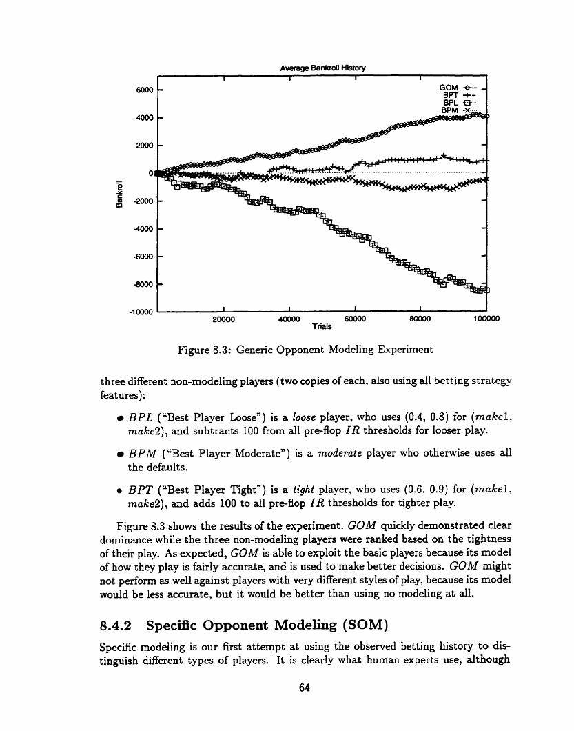
Average Bankroll History

BPL -0- +- 1

-10000 1 I I 1 1 I 20000 40000 60000 80000 1OOOOO

Trials

Figure 8.3: Generic Opponent Modeling Experiment

three different non-modeling players (two copies of each, also using al1 betting strategy feat ures ) :

BPL ("Best Player Loosen) is a loose player, who uses (0.4, 0.8) for (makel, makeZ), and subtracts 100 from al1 pre-flop I R thresholds for looser play.

BPM ("Best Player Moderate") is a moderate player who otherwise uses dl the defaul t S.

a BPT ("Best Player Tight") is a tight player, who uses (0.6, 0.9) for (make l , rnake2), and adds 100 to al1 pre-flop I R thresholds for tighter play.

Figure 8.3 shows the results of the experiment. GOM quiddy demonstrated clear dominance while the three non-modeling players were ranked based on the tightness of their play. As expected, GOM is able to exploit the basic players because its model of how they play is fairly accurate, and is used to make better decisions. GOM might not perform as well against players with very different styles of play, because its model would be less accurate, but it would be better than using no modeling at all.

8.4.2 Specac Opponent Modeling (SOM)

Specific modeling is our f i s t attempt at using the observed betting history to distinguish different types of players. It is clearly what human experts use, dthough

Average Bankroll History 1 I I I 1

GOM +- BPL e- BpT

20000 40000 60000 80000 1 00000 Trials

Figure 8.4: Specific Opponent Modeling Experiment

our approach is cmde and only captures the essence. We measure action frequencies bâsed on a rough description of context and use these frequencies to appropriately adjust the weight m a y on future actions.

The experiment's focus was on two copies of SOM (specific opponent modeling) with respect to two copies of GOM. Like the previous experiment, the other six players were two copies each of B P L , B PT and B PM. The results can be seen in Figure 8.4.

Very quickly, the two opponent modeling programs asserted their superiority over the non-modeling versions. SOM is able to attain a comparable degree of success to GOM based on observed frequencies rather than a good default model. While we cannot conclude on the basis of this one experiment that there is a statistically significant difference between the two modeling versions, anecdotal evidence is somewhat promising: on IRC GOM achieved a wiMing rate of 0.07 small bets per hand and SOM achieved a winning rate of 0.08 s m d bets per hand.

The advantage of good opponent modeling is clear. Loki with opponent modeling is a noticeably stronger program than without it. However, Our implementation of specific modeling does not appear to produce a significant advantage over generic modeling. We recognize that the ganularity of the context for gathering action frequencies may be so coarse that the error undermines the gain. For example, Loki does not recognize that, for some players, calling a bet is automatic given they have already c d e d a bet previously in that round - the second action contains no in-

formation. Some other variables which rnay make the identification of the context stronger include the previous action, number of opponents and number of callers remaining. However, the number of cases becomes very large so it w ~ u l d seem necessary to somehow combine the action frequencies of "similar" scenarios.

Additiondly the re-weighting system is not adjusted based on the specific oppe nent (which only provides simple frequencies). It would be better if we could preàict how each opponent would handle each specific subcase rather than using our value system for assigning strength/potentiaJ with a simple linear function. For example, some opponents may over-value flush draws, or may find it more irnperative to bet a mediocre hand with low potential. The present re-weighting system itself neglects handling certain information. When a check or cal1 is observed we could infer that the opponent does not have a hand above a certain threshold and can apply an inverse re-weighting function to the weight array. This would prevent Loki from being too pessimistic and would d o w it to bet more often after several checks (currently, since checks are ignored and Loki uses HS,, a checking opponent still poses the same threat as one who has not yet acted).

8.5 Summary

There are several different ways to evaluate Loki's performance, however since self- play is the most controlled, results are easily measured. But, we must always be careful in interpreting the results (such as taking into account the interdependencies between players). With only self-play, it is difficult to measure Loki's strength. To help determine this, we use evidence gathered from play on IRC which suggests that it is better than the average human amateur (at least in multi-player scenarios). In particular, al1 of the evidence indicates that the addition of opponent modeling results in a significant increase in strength.

The performance gain from generic modeling is conclusive, however the further superiority of specific modeling is not so clear. This could be due to the granularity of the data gathering, or how the action frequencies are used in the re-weighting, or because the information is not used in the betting strategy. In fact, we strongly believe that the present ad hoc betting strategy, which was originally designed to allow us to quickly test other cornponents, may be a bottleneck preventing further significant progress. This is witnessed in BotWarz with the relatively good performance of less sophisticated cornputer programs, which put more effort into designing a (rule-based) betting strategy. It is dso evidenced by the ease with which strong human players can take advantage of Loki in short-handed play (too many head to head situations against better players).

Chapter 9

Conclusions and Future Work

Loki successfdly demonstrates beneficial opponent modeling in a high-performance game-playing program. In closed self-play experiments it was clearly beneficial to use modeling, and the results from IRC play are also promising. However, it does not necessarily follow that it will be equally successful in games against strong human players. Humans can be very good at opponent modeling, and less predictable than the playen in these experiments.

In our self-play experiments, we have not yet investigated modeling opponents who vary their strategy over tirne. There are also many other interesting questions to be addressed. Our approach was a first approximation using an intuitive approach, and the major benefits came [rom the introduction of the weight m a y (and the re-weighting). The enumeration dgorithms for hand evaluation are well suited to this expression of opponent modeling, allowing it to be a very usefd asset to the accounting systern.

The overall performance was hampered by the ad hoc betting strategy. In fact, many aspects of Loki were a tradeoff between usefdness and correctness - in many places we selected the simple (and cost-effective) approach for its reasonable approximations. Provided the error is not one-sided we should see an amortizing effect. We have not actudly examined what the error is in our many approximations, but it is not worth the effort until it is a limiting aspect of play. Since we plan on replacing the betting strategy with something less dependent on expert des, it is not worth examining the benefits of particular features. Similady, we feel that Bot Warz or generd IRC play could have had better results had we put more time into the betting strategy. However, this would have amounted to tweaking artificid paramet ers wit hout general applicabili ty.

The betting strategy shodd also use the opponent modeling information. A good approach might be to run simulations to the end of the game using the weight array to randomly select "reasonable" opponent hands (and to weight the results as in our enumeration techniques). The specific opponent information could then be used to predict opponent actions in the simulations, resulting in estimates of the expect ed value for each of our options. Presurnably, strategies such as check-raising or bluffing would emerge naturally. For example, blufiing may turn out to be the best action in

a situation where we recognize that our opponent is Iikely to fold. The specific opponent modeling program (SOM) was hampered by the crude

method used for collecting and applying observed statistics. Much of the relevant context was ignored for simplicity, such as the previous action taken by a player. -4 more sophisticated method for observing and utilizing opponent behavior would allow for a more flexible and accurate opponent model.

The re-weighting system could be adjusted, such as inverse re-weightings for passive actions like checking/calling. Presently, every witnessed action leads to the o p p e nent's average hand getting Ustronger". If we considered upper thresholds on actions implying some weakness, like checking and cding, we could approprïately re-weight their weight may. Specific modeling could dso observe variance, or the consistency the opponent exhibits in their behavior. This information could be used in the re- weighting function instead of the simple linear function we use ( with a fixed O).

Poker is a complex game. Strong play requires the player to handle al1 aspects of the game adequately, and to excel in several. Developing Loki seems to be a cumulative process. We improve one component of the program until it becomes apparent that another aspect is the performance bottleneck. That probtem is then tackled until it is no longer the Iimiting factor, and a new weakness in the program's play is revealed. We have made an initial foray into opponent modeling and are pleased with the results, although it is fax from a completed subject.

Wherever possible, the project should be driven to remove whatever human expert information is used. Betting strategy is clearly a major component that needs to be addressed. However, there are other candidates such as more sophisticated opponent modeling. Event ually, more sophist icated simulations for leaniing good pre-flop play could be based on Loh's post-flop playing ability.

Concepts such as hand strength and potential are appropriate for any poker variant. While parts of Our implementation, such as the weight array, may be specific to Texas Hold'em, Our ideas are easily mappable to other variants.

1s it possible to build a prograrn which is the best poker player in the world? Certainly we can construct a program which h a a very strong mathematical basis and nuis within the real-time constraints. It is also clear that some form of opponent modeling (in addition to other advanced features) are necessary to beat the better players. However, it is not clear how difficult it will be to build and maintain opponent models that are sufliciently detailed and context sensitive. While we are probably close to a prograrn which can win money in most typicd low-limit casino games, we are far from the lofty goal of being the best in the world.

Bibliography

H. J. Berliner, G. Goetsch and M. S. Campbell. Measuring the performance potential of chess programs. Artificial Intelligence, 43(l) : M O , April 1990.

D. Billings. Cornputer poker. Master's thesis, University of Alberta, Dept. of Computing Science, 1995. http://www.cs.ualberta.ca/Ngarnes/poker.

D. Billings, D. Papp, J. Schaeffer, D. Szafron. Opponent modeling in poker. In AAAI-98 Proceedings, pages 493-499. The MIT Press, 1998. http://www.cs.ualbert axa/-gamesfpoker.

D. Billings, D. Papp, J . Schaeffer, D. Szafron. Poker as a testbed for AI research. In Robert E. Mercer and Eric Neufeld, editors, Ad- vances in Artificial Intelligence, pages 228-238. Springer-Verlag, 1998. http://www.cs.ualberta.ca/-games/poker.

D. Carmel and S. Markevitch. Incorporating opponent models into adversary search. A A A 1, pages 120-125, 1996.

N. Findler. Studies in machine cognition using the game of poker. Communica- tions of the ACM, 20(4):230-245, 1977.

N. Findler. Computer mode1 of gambling and bluffing. IRE Transactions on Electronic Cornputers, EC-10(1):5-û, March 1961.

N. Findler, H. Klein, W. Gould, A. Kowd, and J. Menig. Studies on decision making using the game of poker. Proceedings of IFIP Congress 1971, pages 1448-1459, 1972.

H. Iida, 1. Kotani, J.W.H.M. Uiterwijk, and H.J. van den Herik. Gains and risks of OM search. In H.J. van den Herik and J.W.H.M. Uiterwijk, editors, Aduances in Computer Chess 8, pages 153-165, Maastricht, The Netherlands, 1997. Department of Computer Science, Universiteit Maastricht.

D. Koller and A. Pfeffer. Representations and solutions for game- theoretic problems. Artificiaf Intelligence, 94(1-2): 167-215, July 1997. http://robotics.Stanford.EDU/-k01ler/ papers/galapaper.html.

H. W. Kuhn. Simplified tw-person poker. In H. W. Kuhn and A. W. Tucker, editors, Contributions to the Theory of Games I, pages 97-103. Princeton Uni- versity Press, 1950.

J. F. Nash and L. S. Shapley. A simple three-person poker game. In H. W. Kuhn and A. W. Tucker, editors, Contributions to the Theory of Games I, pages 105-1 16. Princeton University Press, 1950.

[13] D. Sklansky. The Theory of Poker. Two Plus Two Publishing. Las Vegas. SV, 1994 3rd ed-

[14] D. Sklansky and M. Malmuth. Hold'em Poker for Advanced Players. Two Plus Two Publishing, Las Vegas, NV, 1994 2nd ed.

[15] N. Zadeh. Winning Poker Systems. Prentice Hall, Inc., Englewood ClifIs, NJ, 1974.

Appendix A

Pre-Flop Income Rates

These are the computed income rates (* 1000) used for al1 169 distinct hand types (13 paired, (y ) = 78 suited and 13 * (:) = 78 unsuited). Each table is labeled IRz where x is the number of players (hands ded t ) in the simulation (so there are x - 1 opponents). Each entry is indexed IR,[rav][col] and the cards are suited when row > col. This means that for 2 players the income rate for a 3 and 2 of the same suit is I&[3](2] = -279, and for a 3 and 2 of different suits is IR2[2][3] = -331.

In all simulations a pair of aces had the highest income rate (a gain of 2.043 with 7 players, meaning an investment of $1 wodd return a profit of 12.043, on average). In the 7-player simulation, a 2 and 7 of different suits had the lowest income rate (a loss of $0.495 for every $1 invested) and 88 of the 169 different hand types returned non-negat ive income.

There is a strong correlation between these rankings and the preflop hand rankings given in Sklansky and Maimuth [Ml. They break the pre-0op hands into 9 groups, ranked by their strength (cal1 this ranking of hands SM). If we take I R7 (most reflective of the full game they are assuming) and break it into the same number of groups with the same number of hands per group (5 for group 1, 5 for group 2, 6 for group 3, and so on) we note that dl but 16 of the 169 hand types are either in the same group or are only one away. While most of the hands in the middle groups are shifted by one class, the top three groups are virtually identical. Details of the cornparison by groups c a s be found in Table A.4.

The most interesting similarity is that the top two groups contain the same hands but there is only one different hand in the third group. In IRi, KTs (King and Ten of the same suit) replaces JTs (Jack and Ten of the same suit). In fact, there appears to be a trend favoring big cards in IRi. However, any minor discrepancy could be due to the simple-minded approach of the simulations.

Table -4.1: IRz: income rates for 1 opponent

Table A.2: 1%: income rates for 3 opponents

Table A.3: I R7: income rates for 6 opponents

Table A.4: Cornparison between S M and IR7

Group Size Matches in Group Size Matchs in '

IR7 grouping grouping

Appendix B

Expert-Defined Values

Loki uses several hard-coded constants where the optimal value is too difficult to detemine (or we have not invested the effort to determine a better value). They have been selected by a poker expert, Darse Billings, and have not been experimentally validated. They are used as placeholders, and we foresee eventually upgrading the system so that the cornputer can determine proper behavior on its own.

For the post-flop betting strategy, there are only two expert-defined values: makel and male2 ( t hese are absolute constants, 0.50 and 0.85 respectively. not to be confused s i t h Makel and Make2). These are the betting and raising thresholds for EHS', and represent the likely hand strength required for these actions to be profitable.

For the pre-fiop, when the function SetThresholds is called, it is given three parameters: group, tightness and position. The first two parameters are used to retrieve a set of values ([base, increment], one per strategy). Then the function generates a threshold for each strategy using Equation 6.1, which in turn uses position.

probability-play This value is hard-coded at 0.6, meaning when estimating the number of players (for group) we expect 60% of all players, who have not yet acted, to play to the flop.

group: For the pre-flop, we have reduced the number of classifications, based on the number of players, to three groups: 2, 3-4 and 5 or more players. We consider these the most important groupings and the I R rankings for more than 4 players are nearly identical in any case.

a tightness There are three settings (tight, modemte and loose). By default Loki plays with the Zoose setting. Note that all three sets of parameters are relatively tight styles of play. Even the loose set of parameters is considerably more conservative than a typical loose human player.

strategy There are several different pre-flop strategies that we may use: MakeO, CalIl, Makel, Cal12, Make2 and Make4. Each strategy has a different threshold value based on the context, except MakeO which is the folding strategy. The values for Cal11 and Makel are the same, as are the values for Cal12

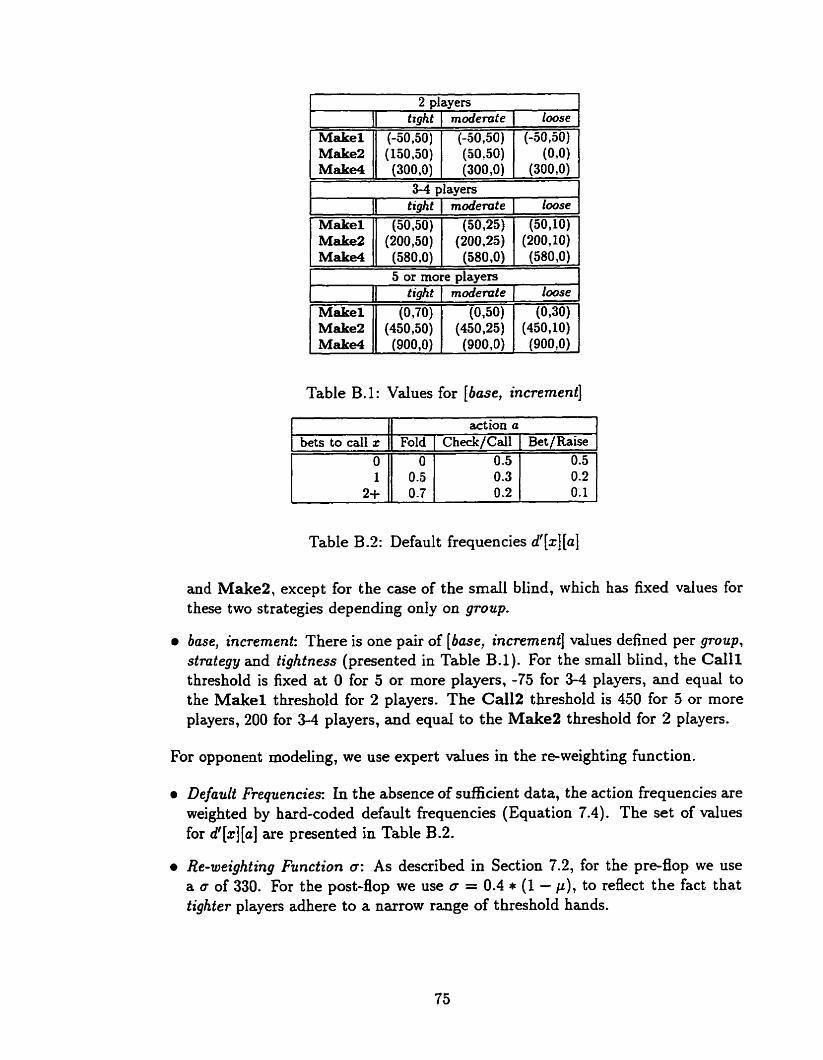
2 players 1

Makel Ma- Make4

Makel Make2 Make4

Table B.1: Values for [base, increment]

Makel M&e2 Make4

I II action a I

i 3-4 la vers

tight

(-50,50) (150,50) (300,O)

5 or more la vers

1 tight (50,50) (200 $0) (580,O)

1 tight

(0,70) (450,50) (900,O)

Table B -2: Default frequencies dl [x] [a]

modemte 1 loose

modemte 1 loose

1 I

bets to cal1 x Fold Check/Call Bet/Raise '

and Make2, except for the case of the small blind, which has fixed values for

(-50,501 (5030) (300,O)

(50,251 (200,25) (580 ,O)

modemte

(0,50) (450,25) (900,O)

these two strategies depending only on group.

(-5030) ( w

(300,O)

(50,10) (200,lO) (580 ,O)

loose

(0,30) (450,lO) (900,O)

0.5 O

base, increment: There is one pair of [base, increment] values defined per group, stiategy and tightness (presented in Table B.l). For the small blind, the Calll threshold is fixed at O for 5 or more players, -75 for 3-4 players, and equal to the Makel threshold for 2 players. The Cd12 threshold is 450 for 5 or more players, 200 for 3-4 players, and equd to the Make2 threshold for 2 players.

For opponent modeling, we use expert values in the re-weighting function.

O

Default Frequencies In the absence of s a c i e n t data, the action frequencies are weighted by hard-coded default frequencies (Equation 7.4). The set of values for dt[x][a] are presented in Table B.2.

0.5

Re-oeighting Function O: As described in Section 7.2, for the pre-flop we use a o of 330. For the post-flop we use c = 0.4 * (1 - p ) , to reflect the fact that tighter players adhere to a narrow range of threshold hands.

Appendix C

Glossary

This is a glossary of both technicd terms (indicated with tt.) and poker jargon used in the thesis. Many of the poker term definitions are based on selected excerpts from the recgambling Glossary of Poker tenns, used by permission of the main author, John C. Hallyburton, Jr.. http://www.conjelco.com/faq/rgpgloss~.

Action F'requency: n. tt. The frequency a certain opponent makes a certain action in a certain context - based on inter-garne statistics.

r Active Player: n. A player who is still in the pot.

Ante: n. A small bet d l players are required to make before a hand is dealt. Not all g m e s have an ante. Related terms: blind.

Bankroll: n. Current total garnbling funds available. To be distinguished from the current money you happen to have on the table. See also: stake.

Bet: v . To put money into the pot, pursuant to the mles of the garne, thus maintaining a chance of winning the pot.

Bet For Value: v. Betting a hand that, in the long nui, is expected to win more than it loses. Antonym: bluff.

Bettor: n. In a given round, the f i s t person to put money in the pot.

Big Blind: n. A blind bet, usually a raise of an earlier blind which would be cdled the small blind. In limit poker, the big blind is u s u d y the size of the minimum bet on the first round of betting.

Blind: n. A mandatory bet made by certain player(s) u s u d y Sitting left of the button before each new hand is dealt. Used in place of, or in conjunction with, antes. See also: ante, big blind, small blind.

r Bluff: n. A bet or raise made with a poor hand, hoping that the remaining active player(s) will fold. Can also be used as a verb.

Board: n. The exposed cards in Hold'em. Also called board cards. See also: community cards.

0 Button: n. A distinctive token held by the player sitting in the theoretical dealer's position (when the dealer is not a player in the game). The button rotates around the table so that every player has an opportunity to be the last to act. "The button" can refer to the player who currently has the button.

C d : v . To put in to the pot the minimum arnount of rnoney necessary to continue playing.

Caller: n. One who c d s . Sometimes used collectively, as in '3 callers."

0 Cap: v. To cap the betting is to make the last permitted raise in a round. In this case, the betting is said to have been capped.

0 Check: v. To bet zero, when it is legal to do so. Frequently a sign of only a fair hand.

0 Check-Raise: v . To check initially, then raise a bet made later on in the same betting round. Frequently a sign of strength, but may be a bluff. See also: sandbag.

Chip: n. A gaming token used in place of cash for convenience in handling and counting. The standard form of cunency in most casinos.

Community Cards: n. Cards that are available for every player to use in making a hand. Usually dedt face-up somewhere in the middle of the table. See also: board.

0 Deuce: n. A two.

Draw: n. [l] A class of poker games characterized by players being dealt 5 cards face-down and later having the opportunity to replace sorne of the original 5. "Draw poker" and "Five-card draw" are examples of usage.

Draw: n. [2] In Hold'em games, the set of cards that will be dealt later can be collectively called "the draw ."

0 Draw: v . To discard some number of cards and have dealt an equal number of replacement S.

Early Position: n. Being one of the first players to act in a betting round. See also: middle position, late position.

Effective Odds: n. A rehement to pot odds which includes estimated extra winnings and cost to see more than one card. The ratio of the expected winnings, when you make your hand, to the cost to play. Used when considering a hand with a high potential given more than one card to corne.

0 EHS: n. tt. Acronym for effective hand strength: the probability of being the strongest hand in the future (i-e. using PPOT and NPOT) . EHS' is an optimistic version which ignores NPOT (used when EHS is considered for a betting decision instead of for a calling decision).

0 Face Card n. A jack, queen or king (a card with a face on it. not joker).

Face-Down: adj. Specifies a card that is known only to the owning player (e.g. your hole cards in Hold'em).

0 Face-Up: adj. Specifies a card is that is known to al1 players (e.g. community cards or board).

a Field Array: n. tt. The average of the nomalized weight anays of ail oppe nents.

First to Act: n. First active player following the button.

0 Fixed Limit: n. A betting structure where the arnount of each bet is a specific fixed quantity. Usudly specified as A-B, where A is the amount to bet in the first few betting rounds and B (larger than A) is the amount bet in the later rounds. Related terms: flat limit, no limit, pot limit, spread limit.

Flat Lirnit: n. A variant of fixed lirnit where all bets are the same amount.

0 Flop: n. In Hold'em, the first three community cards, dealt simultaneously.

Flush: n. A poker hand consisting of five cards al1 of the same suit.

Flush Draw: n. Four cards of the same suit ( L e . missing one card to make a flush).

Fold: W . To decline to cal1 a bet, thus dropping out of a hand.

0 Four of a Kind: n. A hand containing dl four cards of the sarne rank.

a Free Card: n. A card dealt after all players checked in a betting round.

Full House: n. A hand consisting of three of a kind and a (different) pair.

GOM: n. tt. Acronym for generic opponent modeler: a version of Loki that uses default action frequencies for al1 opponents (the re-weighting system is the same for all opponents). GO M' is a later version that uses additional betting strategies like check-raising. Compare: SOM.

Hand: n. [l] A player's hand is the set of cards that only they may use at the showdown. In Texas Hold'em, a player's hand is their set of hole cards.

0 Hand: n. (21 One full game of poker ( i . e . from the blinds or ante until the pot is awarded). See also: trial.

Wgh C d : n. The weakest poker hand, 5 unmatched cards.

Hit: v . To make a hand or catch a card or cards that improves one's hand (e.g. you hold 2-3-4-6 and a 5 is dealt, giving you a straight). Antonym: miss.

0 Hold'em: n. [1] Generic name for a class of poker games where the players receive a certain number (2 t o 4) of hole cards and 5 community cards. Usually there are betting rounds after dealing the hole cards, then after dealing 3 face- up cards (fiop), after dealing a 4th face-up card (turn) and finally after dealing a 5th face-up card (river).

O Hold'em: n. [2] When used in the specific sense (e-g. 'We're playing Hold'em") the term usually refers to the game of Texas Hold'em.

O Hole Cards: n. In certain poker variants, such as Hold'em, the face-down cards dealt to each player. Sometimes d e d the hole.

O HR: n. t t . Acronym for hand r a d : the probability of being the strongest hand in the present state, against one random hand. HR, is the hand r d against n hands.

HS: n. tt. Acronym for hand strength: the probability of being the strongest hand in the present state. HS, is the hand strength against n opponents.

Immediate Odds: See pot odds.

O Implied Odds: n. A refinement to pot odds which includes money not yet in the pot. Considers the ratio of estirnated extra winnings, when a player foms a good hand, to the present cost to c d .

O In: adj. Still eligible to win the pot. '17m in" is often spoken as one calls.

Inside Straight: n. Four cards to a straight, where only one rank will complete the hand. For example, 4-5-68 is an inside straight since only a 7 will complete the hand. Compare: open-ended straight.

0 Kicker: n. In hands containing pairs and three of a kind, the highest card not matched. In drôw games, sometimes a card kept for deception purposes.

Late Position: n. For a particular betting round, a player who does not have to act until most of the other players have acted. See also: early position, middle position.

a Limit Poker: n. A poker gôme wherein the amount to be bet is fixed, or at most variable within a prescribed minimum and maximum. Antonym: no-limit poker. See also: fixed limit.

Loose: adj. PIaying more hands than the norm. Antonym: tight.

Middle Position: n. Betting positions approximately halfway around the table from the first player to act. See also: early position, late position.

Make: v . To make a hand is to receive cards that improve one's hand. See also: hit.

Miss: v. To receive a card that does not improve one's hand. Antonym: hit .

No-Limit Poker: n. A game where there is no maximum bet; a player can wager any amount (perhaps above some minimum) up to whatever money is on the table in front of him. Antonym: limit poker. See also: h e d limit.

NPOT: n. t t . Acronym for negative potential: the probability of fding behind given that we are ahead (approxirnately, the percentage of upcoming cards that help our opponents). NPOTi is the one card potential and NPOTz is the two card potential. Compare: PPOT.

Off-Suit: adj. Not of the same suit. "1 held A-Q off-suit" or "The flop was 10-6-2 off-suit." When speaking of 5 or more cards, then not al1 of the same suit ( i e . no flush).

One Pair: n. The second weakest poker hand. It contains two cards of the same rank and 3 unmatched cards (kickers).

Open: v . Make the first bet in a hand, especially in draw poker.

Open-Ended Straight: n. Four cards to a straight which can be completed by drawing a card at either end. E.g. 6-7-89 is an open-ended straight. Compare: inside straight .

Out: n. A card that will improve your hand, often substantially. A hand with many outs is preferable to a hand with only a few. E.g. with a flush draw in diamonds, any diamond is an out.

Out: adj. Folded, ineligible to bet or win this hand. "17m outn is often a synonym for "1 fold."

0 Overpair: n. In Hold'em, a pair in the hole that is larger than any cornmunity card on the board.

a Pair: n. Two car& of the same r d .

Position: n. One's location in the betting sequence, relative to the players still in the hand. First position is first to act.

Post-Flop: n. In Texas Hold'em, the rounds foilowing the turning of the flop cards ( i .e. the flop, turn and river). Compare: pre-flop.

Pot: n. The total arnount of money bet so far in a hand.

a Pot Limit: n. A game where the maximum bet is determined by the size of the pot at the time. Note that a player wanting to raise first calls the bet, then totals the pot to determine the maximum amount he c m raise. See dso: fixed limit . Pot Odds: n. The ratio of the money in the pot to the amount of money to c d . Often used with respect to the potentid of your hand to determine if a pot offers enough reward to pay to see the next card.

a PPOT: n. tt. Acronym for positive potential: the probability of pulling ahead given we are behind (approxirnately the percentage of upcoming cards that male us a sure winner). PPOTl is the one card potential and PPOT2 is the two card potential. In some cases where we need a very quick estimate, we use PPOT, (for cmde). It uses some fixed rules to quickly determine an estimate of PPOTl. Compare: NPOT.

a Pre-Flop: n. In Texas Hold'em, the round preceding the tuming of the flop cards, where there are no cornmunity cards. Compare: post-flop.

a Pure Bluff: n. A bluff made with a minimal chance of winning, usually on the final round with no further cards to corne.

Raise: v . To wager more than the minimum required to call, forcing other players to put in more money as well.

Raiser: n. One who raises.

a Represent : v . Implying, by one's bett ing style, that one has a particular hand.

a Reraise: v . To raise after an opponent has raised.

Reverse Implied Odds: n. A refinement to pot odds which includes extra cost to play the hand. Considers the ratio of the present pot to the estimated extra cost to play to the end of the hand.

Re-weight: v . t t . The process of taking an observed action (and its action frequency) and applying a transformation function to adjust the weight array to represent a more likely distribution of hands held by the opponent.

O River: n. The last card dealt in a hand of Hold'em-

0 Roll: v . In some variants, instead of deding extra cards the rules rnay call for players to roll over some face-down cards (tum them face-up).

Round: n. A poker variant is composed of several rounds. In each round, players take some action (such as being dealt a new card) and then proceed to a betting series. E.g. Texas Hold'em has four rounds (pre-flop, Bop, turn and river).

Royal Flush: n. An ace-high straight flush, the best possible hand in regular poker.

Sandbag: v . Playing a strong hand weakly. See also siowplay, check-raise.

Script: n. tt. The definition for a poker variant presented as a sequence of events (e.g. each player receives t cards face-down, followed by a round of betting, etc.).

Semi-Bluff: n. A bet with a weak hand that has good drawing potential and is Likely to win if it hits (e.g. a flush draw with no pair is often a good semi-bluffing hand). Can be used as a verb.

Session: n. A contiguous series of hands (games oi poker).

Short-Handed: adv. Playing against only a few other opponents (usually 2-4 players total). Opponent modeling is much more important.

0 Showdown: n. The point at the end of the hand where all active players reveal their cards and the pot is awarded to the winner(s).

Showdown Odds: n. A refinement to pot odds which considers the ratio of the estimated winnings to the estimated cost to play to the end of the hand.

Slowplay: u. To play a strong hand weakly, by checking instead of betting or by cd ing instead of raising. Usually done to win extra bets by keeping more players around for future rounds of betting. See also sandbag.

Small Blind: n. In games with two blinds the first blind is the small blind because it is u sudy one-half (or less) the second or big blind.

SOM: n. tt. Acronyrn for specific opponent modeler. a version of Loki that ac- cumulates statistics for each opponents to calculate action frequencies which âre used to appropriately re-weight based on observed actions. SOM' is a later version that uses additional betting strategies like check-raising. Com- pare: GOM.

Spread Limit: n. A variation on fixed limit wherein the minimum and maximum bets are different. A 1-4-8 game allows bets from 1 to 4 in the early rounds and 1-8 in the last round. A 1-4-8-16 game allows bets from 1 to 4 in the early rounds, 1 to 8 in the next-to-last round, and 1 to 16 in the last round.

O Stake: n. The amount of money a player is willing or able to play with in a given session. Compare: bankroll.

Steal: u. To win the pot by bl&g.

Straight: n. A hand consisting of 5 cards in sequence but not in suit.

Straight Draw: n. A four card straight. See also: inside straight, open- ended straight.

0 Straight Flush: n. A hand consisting of 5 cards in sequence and the same suit.

0 Suited: n. Two or more cards al1 the same suit. Antonym: ossuit.

a Table: n. The set of players playing together.

Tell: n. Any personal mannerisms that reved the quality of one's hand. E.g. constantly looking at one's hole cards is often a tell of a poor hand. (Some players, knowing this, will a t times check their hole cards when they have a great hand and don't need to look).

Texas Hold'em: n. A Hold'em game where players receive two hole cards and may use zero or more of them, together with 5 board cards, to make their hands. See Hold'em.

Three of a Kind: n. Three cards of the same rank.

Tight: adj. Playing fewer hands thao average. Antonym: loose.

0 To Call: adj. The amount that the current player must cal1 to continue playing; it is a factor of the previous betting action this round. E.9. if the current player has called the first bet of $10 but there has since been a raise of $10 then it is "$10 to cdln for that player. Compare: to go.

a TO Go: adj. The current betting level, as in "$20 to gon rneaning every player must contribute $20 (total) or drop. A $10 raise would then make the pot "$30 to go."

Top Pair: n. In flop garnes, having a hole card that matches the highest card on the board.

a Trey: n. A three.

O nial: n. tt. In the self-play tournaments that Loki uses, a trial is one particular instance of a hand. For each particular distribution of cards, the hand is replayed ten times (trials), shuffling the seating arrangement each time to reduce the luck element .

O Turn: n. The fourth community card in Hold'em.

0 Two Pair: n. A poker hand which contains two pairs of different ranks and one kicker-

Weight Array: n. tt. The component of an opponent mode1 that is used to obtain a weighted sum in the hand evaiuation algorithms. For each opponent there is a weight for each possible combination of hole cards. This weight a p proximately represents the conditional probability that they would have played in the observed maaner (given that hand). See also: re-weight.

Wild Card: n. A joker or standard card that, by player agreement and/or dealer's choice, can be used to represent any card desired.

O World Series of Poker: n. A series of several different poker games with relatively large entry fees, culminating in a $10,000 entry-fee nelimit Hold'em tournament, the winner of which is crowned the World Poker Champion. Spon- sored by Binion's Horseshoe Club in Las Vegas.

IMAGE EVALUATION TEST TARGET (QA-3)

A P P t l E D J IMAGE. lnc 1653 East Main S m t - -- - - Rochesîer. NY 14609 USA -- -- - - Phone: 71 61482-0300 -- -- - - F a 71 6/2-5989

O 1993. AQOlied Image. Inc.. W RQhb Reserved

Documents

· Abstract Poker provides an excellent testbed for studying decision-making under conditions of uncertainty. There are many benefits to be gained from designing and experimenting