Abstract - Petroglyph Project Analytics

Utilizing Linear Planning and Scheduling for Project Control and Claims Avoidance

Joanna Alvord, PSP, PMP, Project Controls Manager, HDR Engineering, Inc.

Lorne Duncan, Partner, Integrated Project Services

Abstract

March charts (also known as time-distance charts) have been widely used in linear construction

projects such as heavy civil, rail, pipelines and tunnels. Historically these march charts have

been hand drawn, prepared in Microsoft Excel or in created in a drawing program such as

AutoCAD™. In recent years the development of software such as TILOS™ to plan and control

linear projects, with the ability to create critical path schedules, has made this task much easier.

Linear planning software connects the schedule data to the geography of the ROW, easily

identifying construction sequencing, constructability issues, preferred distance between the

crews on the site thus assisting in the project risks identification and mitigation. It communicates

more information because the distance related data is assigned to each task and effectively

displayed in the report. Using linear tools such as TILOS allows you to exchange data between

Primavera, MS Project or Excel.

In this session, the advantages of using linear scheduling method to plan, schedule and control

linear projects over traditional methodologies will be reviewed and examples provided. An

emphasis will be placed on the benefits of using this software for project control and claim

avoidance.

Introduction

Linear projects involve the continuous movement of activities along the length of an alignment

or right-of-way. Some examples would include highway, pipeline, railway and high voltage

transmission line projects. Linear projects are characterized by the repetition of each activity

along the length of the project. The rate of progress of each crew is critical and is evaluated to

ensure that adequate spacing between activities is maintained. Typically, the sequence of

activities is not a concern but rather optimizing the productivity rates to minimize the total time

in the field (Duffy, 2009)

Traditional scheduling methods used for linear construction projects have been either simple bar

chart as developed by Henry Gantt during World War I or a critical path method (CPM)

schedules first developed by DuPont in 1957. (Duffy,2009). Gantt charts, while easily

developed and understood, don’t convey sufficient information control a project. CPM

scheduling methodology was originally developed for facilities type of jobs where the project is

broken down into a complex series of sequential discrete activities (Duffy, 2009) of these

©2010, Joanna Alvord and Lorne Duncan -2-

Originally published as a part of PMICOS 2010 Annual Conference

solutions provide opportunities to develop a series of activities that are logically connected in a

sequence from project start to finish. While these tools are very powerful, they are better

designed for the construction of facilities (i.e., power generating stations, refineries and chemical

plants) and are not adequate for the constructability issues and demands of building linear project

such as a pipeline, rail system or roadway.

Repetitive projects can be classified into two categories: point based and alignment based

(Duffy, 2009). A point based project is based on the Line of Balance (LOB) method developed

by the U.S. Navy in the 1950’s to optimize production of units in an assembly plant (Duffy

2009, Johnson, 1981). ). O’Brien (1975) introduced the Vertical Production Method (VPM) to

schedule the repetitive nature of multi-storey buildings as crews move up from floor to floor.(

March charts (also known as Time-Distance charts) have been widely used in linear projects,

particularly in Europe and the U.K. This methodology is newer to the Americas, but is rapidly

gaining widespread acceptance. March charts are often hand drawn, prepared in Microsoft

Excel or in a drawing program such as AutoCAD. Linear planning and scheduling software that

automates development of the plan and progressing is relatively recent (approximately the last

15 years). Key advantages of march charts are that the schedule is connected to the geography of

the ROW and any constructability issues that are important to the project.

THE BASICS

DIFFERENCES BETWEEN CPM AND LINEAR SCHEDULES

CPM schedules are familiar to anyone that has planned and executed a project. The planner

creates a series of activities based on the project execution plan and then logically connects these

activities (Finish-Start, Start-Start, Finish-Finish and Start-Finish). Resources can be added to

each activity schedule and resource loading can be easily displayed. In order to maintain crew

sequencing in a linear project, the planner ensures that each activity is connected to its successor

by a Start-Start and a Finish-Finish relationship. A typical Gantt chart for a pipeline job is

shown in Figure 1.

Figure 1 Traditional Gantt Chart



This Gantt charts clearly shows each activity with its start and end date and progress is shown

on the Gantt chart as the percent completed for each task. In a linear project reporting reporting

that a crew is 45 % complete is quite meaningless because these traditional tools assume that

progress is from start to finish and no connection exists between progress and the geography of

the ROW. The ability to include crew moves, permitting delays, environmental restrictions and

other construction issues is simply not possible.

A march chart on the other hand displays the same crews as a series of lines moving along the

ROW. As with the CPM method, each crew is logically connected to its successor with Start-

Start and/or Finish-Finish relationships. Completed sections are easily identified with crew

moves, crossings and environmental windows visible on the march chart. Using the same

example as before, a march chart will clearly display what 45% of the ROW has been completed

by the bending crew and how any moves or ROW access issues have impacted the progress of

the project.

A typical march chart (Figure 2) in its most basic form shows each crew represented by a

different line type or shape. Usually distance along the ROW is horizontal and increases from the

left to the right. Time is typically represented vertically, increasing from bottom to top (although

it can just as easily be shown increasing top to bottom). It should be noted that the orientation of

the time and distance axes is a matter of personal preference and can easily be switched in the

software.

The advantage of march charts is immediately obvious as you can determine the location of each

crew at any particular point in time. Any issues associated with crew productivity rates are also

readily apparent. For example, the red arrow in Figure 2 indicates that based on the productivity

of each crew, the lower-in crew will overtake the ditching crew between KP 25+000 and

30+000, which was not obvious in the Gantt chart view (Figure 1).



Figure 2 Simple March Chart

In a march charts the slope of the activity indicates the relative productivity rate for the crew.

The steeper the slope, the slower the crew is moving (because more time is spent and less

distance is completed). Non-work periods such as scheduled days off or work stoppages appear

as vertical segments on the crew line. A vertical line indicates that time is passing but the crew

is not moving. Figure 3 shows an example where the grade crew is moving slower (468 m/day)

than the Haul and String crew (600m/day) with each crew working a 6 day 10h shift rotation.

The green bars across the march chart and the short vertical jumps in each crew, indicate the day

off each week. This march chart shows that grading has to start 18 days ahead of hauling and

stringing in order to keep these crews from overlapping.

The productivity rates that are displayed are calculated automatically by the march chart

software based on duration and length of each task.

For clarity and ease of explanation, all of the following examples in this guide will show only a

few representative pipeline crews. Typically, each crew is assigned to a different layer of the



march chart so that the planner can display one or many crews simultaneously, by activating the

layers.

Figure 3 Productivity Rates and Slope

CONSTRUCTABILITY ISSUES

With a basic understanding of these march chart elements, a march chart can be further

enhanced to display any other critical element of your project. These can include the ROW

profile, crossings, environmental restrictions and land acquisitions. Other elements such as

vegetation type, soil type and rainfall data can also be included on the march chart. The amount

and type of information shown on a march chart is determined by the project team.



ROW PROFILE

The ROW profile is important in developing the hydro-test plan and to determine productivity

rate changes based on elevation (discussed later in the speed profiles section). Most profile data

(LIDAR or survey) is available in a spreadsheet format and can be easily imported into a profile

diagram using the import function of the march chart software to generate the ROW profile as

seen below in Figure 4.

Figure 4 Elevation Profile and Restricted ROW Access



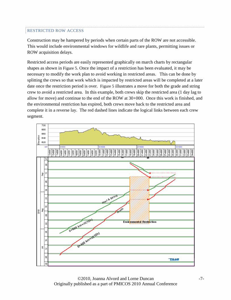
RESTRICTED ROW ACCESS

Construction may be hampered by periods when certain parts of the ROW are not accessible.

This would include environmental windows for wildlife and rare plants, permitting issues or

ROW acquisition delays.

Restricted access periods are easily represented graphically on march charts by rectangular

shapes as shown in Figure 5. Once the impact of a restriction has been evaluated, it may be

necessary to modify the work plan to avoid working in restricted areas. This can be done by

splitting the crews so that work which is impacted by restricted areas will be completed at a later

date once the restriction period is over. Figure 5 illustrates a move for both the grade and string

crew to avoid a restricted area. In this example, both crews skip the restricted area (1 day lag to

allow for move) and continue to the end of the ROW at 30+000. Once this work is finished, and

the environmental restriction has expired, both crews move back to the restricted area and

complete it in a reverse lay. The red dashed lines indicate the logical links between each crew

segment.



Figure 5 Restricted Access Showing Move Around

CROSSINGS

Once the environmental or land restrictions have been established on your march chart, the next

step is to identify crossings. Crossing types can include foreign utilities, roads, rail or water and

are important features to locate on your march chart. The method of crossing will be dependent

upon the type of crossing. Water crossings usually require an open cut (if permissible under the

environmental guidelines) or will utilize a HDD (Horizontal Directional Drill). Most roads and

rail crossings utilize some type of bore method while foreign utilities are exposed using a

hydrovac. Each type of crossing can be color coded on the march chart for quick and easy

identification.

Figure 6 (below) shows a highway (at KP 1+793) shown in grey and a blue river crossing (KP

29+690) on the march chart.



Figure 6 Road and River Crossings

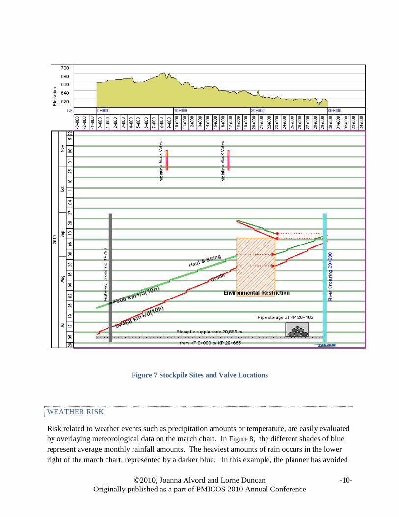
STOCKPILE LOCATIONS AND VALVE SITES

Virtually any information that is considered important can be inserted into the march chart. The

following example (Figure 7) shows the stockpile location (KP 26+102) and the supply zone for

this pipe (KP 0+000 to KP 29+655). It is interesting to note that non-linear structured tasks

(such as mainline block valves) can also be shown on a march chart. The two valves shown in

Figure 7 are represented by a series of rectangular shapes indicating different stages of

installation from civil to mechanical to instrumentation and telemetry. Other non-linear features

that can be added to a march chart would include hot bends (with delivery dates) and detailed

HDD activities. Pump stations can also be represented as rectangular activities that can be

progressed as well. In this regard, a march chart is able to represent both linear and non-linear

components, providing an overview of the entire project.



Figure 7 Stockpile Sites and Valve Locations

WEATHER RISK

Risk related to weather events such as precipitation amounts or temperature, are easily evaluated

by overlaying meteorological data on the march chart. In Figure 8, the different shades of blue

represent average monthly rainfall amounts. The heaviest amounts of rain occurs in the lower

right of the march chart, represented by a darker blue. In this example, the planner has avoided



working in this area during high rainfall thus reducing the risk of heavy rain impacting

construction.

Figure 8 March chart showing monthly average rainfall data.



OTHER FEATURES

SPEND PROFILES AND RESOURCE HISTOGRAMS

Spend profiles and resource histograms are simple to create once costs are added to the labour,

equipment and materials used in the march chart. Figure 9 illustrates an example where the

weekly cost per crew and the total cumulative cost is presented in a histogram and table. It is

also possible to display the resource histogram per week (month or day) to determine camp

requirements. Spend profiles are a function of time and are therefore displayed parallel to the

time axis of the march chart. It is also possible to create a spend profile parallel to the distance

axis showing the cost per section of the pipeline. Any changes to the march chart (such as crew

moves) automatically create a change to the spend profile.



Figure 9 Weekly Spend Profile (per crew with weekly and cumulative totals)

APPLYING WORK AND SPEED PROFILES TO CREWS

Most estimates, schedules and march charts assume a consistent productivity (or work) rate for

each pipeline crew along the ROW. This productivity factor is then applied for the entire length

of the ROW to determine the duration of each crew. Applying a constant productivity rate to a

crew doesn’t account for changes in profile, soil, terrain (muskeg versus mineral soil conditions)

or vegetation types.

For example, a logging crew that has a productivity rate of 2000 m/day would require 15 days to

complete a 30 km ROW. While this provides a rough estimate it doesn’t account for

productivity rates based on changes in vegetation types or whether there is logging required in

certain areas (for example an old burn area that doesn’t have salvageable timber).

The following examples shown in Figure 10 and Figure 11, illustrate the difference when a

vegetation classification system is used to define the productivity rates for logging and clearing

crews in a Northern ROW. In this example the vegetation data and productivity rates for both

crews in a particular location were imported directly into the march chart from an Excel data file

supplied by a survey company.



Figure 10 Logging and Clearing Crews with constant productivity

In Figure 10, we can see that both crews have very similar productivity rates with durations of 25

and 26 days respectively for the logging and clearing crews.

The vegetation index in this example defines the amount of work (area in Ha) and work rate for

each vegetation type along the ROW. Once this data is known and available in a spreadsheet

format, it is easy to apply this index to each crew as shown in Figure 11 below. The first

noticeable change is that the crews are not consistently progressing along the ROW. Each crew

line now reflects a different productivity rate with each change in vegetation type. More

importantly we can see that the duration for each crew has changed significantly. Logging has

decreased from 25 days to 16 days while the duration for clearing has increased from 26 days to

40 days!



Figure 11 Logging and Clearing optimized by vegetation index

This approach could easily be used in any other geographic location where a known variable

impacts the work rate of crews along a ROW. The ability to define productivity in terms of the

ROW conditions will enable you to create a more accurate project plan and spend profile when

compared to simply applying an uniform rate to each crew. Progress can now be applied against

the adjusted crew profiles.

Applying a speed profile to a crew, based on known changes in productivity, creates a more

accurate picture of how the crew is moving along the pipeline ROW as seen in Figure 12.



Figure 12 Crew Speed profile

PROGRESSING MARCH CHARTS

Progressing crews on a march chart requires the start KP, end KP and the date range for each

progress period (based on the inspector field reports) is applied. The exception to using linear

meters for progress would be to count the number of welds, usually back end welds, or the

number of UPI items, such as bag weights.

Figure 13 shows progress for both the grade and the haul & string crews. Progressing is as simple

as selecting a crew by clicking on it, right click and select enter progress. Enter the start and end



date for the progress period and the start and end KP. The march chart software calculates the

physical percent completed based

Figure 13 Progressing Crews in March Charts

upon the amount of work completed divided by the total length of the pipeline. In this example,

grading is 61.02% and haul & stringing is 40.44% complete. It should be noted that the progress

is for the segment starts at KP 0+000 and ends at restricted access area, it doesn’t include the

other two segments for each of these crews.

PROGRESS BAR CHARTS

Progress can also be indicated in a bar chart format where each the progress of each crew is

represented by a shaded bar chart. As progress is applied to a crew the bar chart view is



automatically updated to reflect this progress. In Figure 14, the direction of build is from KP

162+000) to KP 112+000. In this example, the clearing, pioneering and grade crews have

completed the entire length of the spread. haul and string are between 40% and 50% complete

and the automatic welding crew has just kicked off.

Figure 14 Crew Progress Bar Chart

CONCLUSION

The intent of this guide is to provide a comparison of traditional scheduling tools to march

charts and to provide an overview of the how to interpret these charts. This overview described

how to interpret march charts in the simplest form and then increased the complexity by adding

constructability issues such as environmental restrictions and risk such as weather. The ability to

represent non-linear activities (valves and pump stations) on a march chart makes this a very

powerful solution that enables one to view the entire project on one march chart.

Also described was the ability to apply speed and work profiles to connect the productivity rates

to soil, timber or any other factor that will have an impact. Progressing during project execution

is dependent on the input of the crew inspector daily report. Typically the start and end KP for

each crew is recorded daily for progressing the march chart. UPI items and welding may also be

tracked as the number installed or completed.

It should be apparent that march charts are well suited for pipeline construction projects. We

have seen that march charts connect the schedule to the geography and risks of a project in a

manner that is not simply possible using traditional scheduling methods. Hopefully, this guide

has helped you gain an understanding and appreciation of march charts and the potential that is

possible.



References

Duffy, G.A. (2009) Linear Scheduling of Pipeline Construction Projects with Varying

Production Rates. PhD Thesis. Oklahoma State University

Documents

Abstract - Petroglyph Project Analytics