Abstract number: 002-0470

A New Approach for the Production Planning of Flexible Manufacturing Systems Based on

the Concept of Operation Types

Second World Conference on POM and 15th Annual POM Conference, Cancun, Mexico, April 30 – May 3, 2004

Tamás Koltai (corresponding author) Budapest University of Technology and

Economics Department of Industrial Management

1111 Budapest, Műegyetem rkp. 9. T. Bld., Hungary

E-mail: koltai@imvt.bme.hu Phone: 36-1-463-2432

Fax: 36-1-463-1606

Kathryn E. Stecke The University of Texas at Dallas

School of Management P.O. Box 830688, Richardson, Texas 75083-

0688, USA E-mail: KStecke@utdallas.edu

Phone: 972-883-4781 Fax: 972-883-2799

Viktor Juhász Budapest University of Technology and

Economics Department of Industrial Management

1111 Budapest, Műegyetem rkp. 9. T. Bld., Hungary

E-mail: juhaszv@imvt.bme.hu Phone: 36-1-463-2432

Fax: 36-1-463-1606

Peter Várlaki Széchenyi István University

Institute of Informatics and Electrical Engineering

Department of Matematics 9026 Győr, Egyetem tér 1, Hungary

E-mail: varlaki@jgi.bme.hu Fax: 36-1-463-1783

Abstract

Manufacturing systems produce parts to meet demand, either forecast and/or actual. When developing a production plan, an initial question is whether there is enough capacity from the system for the different operations demanded by the production requirements. The paper provides an aggregate capacity analysis model, which can be the basis for aggregate production planning. Aggregation in the paper means that the similar manufacturing operations, which require the same type of machines, are aggregated into operation types. Applying the concept of “operation types”, the variety of the alternative uses of the production capacity can be reduced and a systematic evaluation of capacity utilization and workload balance is possible. The proposed capacity analysis model, can help operation managers to make production planning decisions, make or buy decisions, and can assist when decisions on taking certain orders has to be made. The basic concept of the model is illustrated by a real case example. The paper also highlights some further research possibilities based on the operation type aggregation concept.

2

1. Introduction

Manufacturing systems produce parts to meet demand, either forecast and/or actual. When

developing a production plan, an initial question is whether there is enough capacity from the

system for the different operations demanded by the production requirements. Production

planning for the equipment that performs different operations in conventional manufacturing

systems is more straightforward than in flexible manufacturing systems. In some conventional

systems, the capacity available for production can be determined directly from the available

capacities of the different single-purpose machines, as they can usually perform only a small

variety of operations. (Conventional and manual systems may also contain general-purpose

machine tools.) A system with multi-purpose computer numerical control (CNC) machines

provides additional opportunities to increase system utilization through the machine flexibility,

since each machine can be used for a variety of operations. In this case, it is useful to know if

there is enough capacity of a variety of functional types to perform all of the technologically

different operations. If there is enough capacity of different types, then next, the alternative uses

of the machines for the different operations need to be analyzed. For example, in a combined

system with mixed types (single- and general-purpose) of machines, decisions concerning

whether certain operations should be assigned to the single-purpose machines (or not) can be

considered in order to leave the CNCs free for more complex or special operations.

This type of problem is found in production systems that produce several types of parts

requiring technologically different operations on both CNC and conventional machines. For

example, consider the manufacturing system of a particular company, GE Lighting Tungsram,

producing parts for light source production lines. In this system, about 5000 different part types

are produced yearly in small and medium lots. Several multiple axis CNC machines as well as

3

conventional machines are available for production. Some part types can be produced on both

CNC and conventional machines, while others can only be produced on CNC machines.

Consider a GE example of two part types (a bearing block and a driving plate) to be

scheduled for production in a particular time period. The bearing block requires milling with the

following three tools: side mill, face mill, and drilling end mill. It also requires drilling with two

different size drills. These operations can be performed either on a three-axis CNC milling

machine with one mount and requiring 5 tools, or can be performed on three conventional

machines (vertical mill, lathe, and a drilling machine). The driving plate requires a complicated

milling operation with an end mill, which can be done only on the CNC machine. The following

questions need to be addressed by the GE production manager when planning production for the

addition of these two part types to a current production plan for an upcoming period of time:

– Should the CNC machine be used only for the driving plate and the conventional

machines only for the bearing block? If, in this case, there is not enough capacity on the

conventional machines, should certain operation(s) be moved to the CNC machine or instead,

should overtime be scheduled for the conventional machines?

– Can only the CNC machine be used for both part types by loading all of the required tools

for them? If, in this case there is not enough capacity on the CNC machine to perform all of the

required operations, should certain operation(s) be moved to the conventional machine(s) or

instead should overtime be scheduled for the CNC machine?

These questions should be answered considering that

– Production and tooling costs are different on the conventional and CNC machines.

– Overtime costs money.

– Workers at the CNC and conventional machines should have balanced workloads to

avoid dissatisfaction of workers having uneven workloads as well as under-utilized machines.

4

– Some special cutting tools might be in shortage if they are loaded on too many machines

at the same time.

– Flexibility in a production plan is very useful in rescheduling production in the case of

machine breakdowns, because the delay of some parts may delay subsequent assembly

operations.

This small example of two part types demonstrates the real problems that exist when

several hundred part types and all of the machines of the manufacturing system are involved. The

techniques presented in this paper can help companies similar to GE Lighting Tungsram address

such issues.

The paper provides aggregate model for capacity analysis. Aggregation here means that the

similar manufacturing operations, which require the same type of machines, are aggregated into

operation types. Applying the concept of “operation types”, the variety of the alternative uses of

the production capacity can be reduced and a systematic evaluation of capacity utilization and

workload balance is possible.

An easy-to-use mathematical model and graphical illustrations are provided to analyze the

capacity over- and under-utilization of the machines, as well as of the entire system.

Aggregation is a widely used tool in production planning. When some elements of a

production system are treated in an aggregate manner, simpler models can be applied for

capacity, inventory, and production planning. Obviously some information is lost by aggregation,

but at a certain level of decision-making, an aggregate treatment can be sufficient. When

information that is more detailed is required, then the aggregated concepts are disaggregated

and/or a more detailed model is applied. In traditional production planning models, products

and/or facilities are aggregated (Thomas and McClain, 1993). Products using the same setup of

the production process are aggregated into product families and/or products with similar resource

5

consumption are aggregated into product types. When a good production plan and capacity

utilization is determined, a detailed production program can be prepared, in which product types

and/or families are disaggregated into products (see, for example, Johnson and Montgomery,

1974 and Hax and Candea, 1984). Facility-level aggregation means that several different

resources of the production, such as machines, workforce, and materials are considered as a

single resource or facility (see, for example, Holt et al. 1960).

Special-purpose machines perform just a small set of technologically different operations.

In this case, aggregation of machines is approximately equivalent to the aggregation of

operations. In case of multi-purpose CNCs, machines and operations have to be treated

separately, since the operation manager decides on the set of operations a machine has to

perform. This fact was recognized by Niess (1980), who aggregated similar operations into

operation types. Niess developed an algorithm to determine a series of sets of orders for several

production periods. The generated production program provides balanced capacity utilization,

that is, there is no excess capacity over- and under-utilization. Niess applied this method for

conventional production systems consisting of several single- and multi-purpose machines.

To solve the FMS production planning problems, Stecke (1983) proposed a nonlinear

integer production planning model. The size of this model, however, can preclude frequent

application, especially for a large FMS. A hierarchical approach was also proposed by Stecke

(1986), Van Looveren et al. (1986), and Jaikumar and Van Wassenhove (1989) to handle the

increased complexity of FMS production planning. Stecke and Kim (1991) suggest an aggregate

approach to sequence the production of orders for different types of parts in order to balance the

workload for the various machine types.

Production planning of an FMS in an MRP environment was presented in Mazzola et al.

(1989). In this case, part type selection is determined by an MRP system in the rough cut capacity

6

planning phase. For the selected part types, first grouping and loading of machines is solved, then

detailed scheduling is done. Since part type selection is solved independently of the grouping and

loading problem, the complexity of the model is somewhat reduced, but still the solution of real

size models requires efficient heuristics.

The complexity of the capacity analysis of FMSs implies that aggregation could be an

appropriate approach. The technological characteristics of these systems, however, require

modification of traditional aggregation concepts. The capability to perform a large number of

technologically different operations can cause difficulties in production planning as well as

benefits for operation. The main contribution of this paper is to show how the increased

complexity of the capacity analysis of FMSs can be addressed by aggregating operations into

operation types. It is very difficult to solve simultaneously machine pooling, tooling, and loading,

and frequently it is not even necessary. When the manufacturing manager in GE Tungsram would

like to know whether there is enough capacity on the CNC and conventional machines to

manufacture a given set of orders considering certain flexibility and cost objectives, then a

detailed tooling and routing solution is unnecessarily detailed information. Evaluation of the best

possible tooling and routing is required only after decision on the acceptance of the orders. That

is why hierarchical approaches are proposed to solve the production planning problems of FMSs.

When operation types are used, a framework is obtained for the subsequent detailed workload

allocation (during disaggregation). Using the suggested method, the aggregation concept applied

for conventional systems can be extended for FMSs. A key idea is that the focus is on the

requirements of the operation types rather than on the capability of each machine.

The paper is organized as follows. First the basic notation, and the concept of the capacity

analysis model are provided. Next the application of the model for a sample problem based on the

part manufacturing division of GE Tungsram in Hungary is illustrated. The example is followed

7

by sensitivity analysis. It is explained how the change of production requirements and machine

capacities can be analyzed with the help of the presented method. Finally, the main application

areas of the model are summarized.

2. Basic definitions and concepts

A flexible manufacturing system (FMS) is a collection of machines, linked together by an

automated materials handling system and directed by a central computer. An order (for a single

part type) consists of ri parts of type i. Each part type has a finite number of operations. An

operation, oj, is defined by its processing time on a given machine and by the set of cutting tools

required.

A machine visit requires a pallet, a fixture, and whatever is on the fixture. This is usually a

single part, but may also be multiple parts of the same type or multiple parts of several types, in

one or more mounts. Each part type may have a (partial) precedence among its operations.

An operation type, oth, is an aggregated set of all of those operations that can be performed

on the same machines. Let’s consider a part, which requires several milling and drilling

operations. If all of the machines are able to perform all operations, then the manufacturing of

this part requires one operation type consisting of all drilling and milling operations. If, however,

two machines can perform the drilling operations, and just one of the two machines can perform

the milling operations, then the operations are aggregated into two operation types (drilling and

milling).

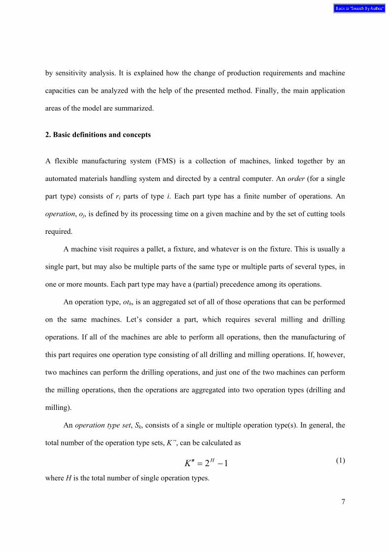
An operation type set, Sk, consists of a single or multiple operation type(s). In general, the

total number of the operation type sets, K”, can be calculated as

(1)

where H is the total number of single operation types.

12 −=′′ HK

8

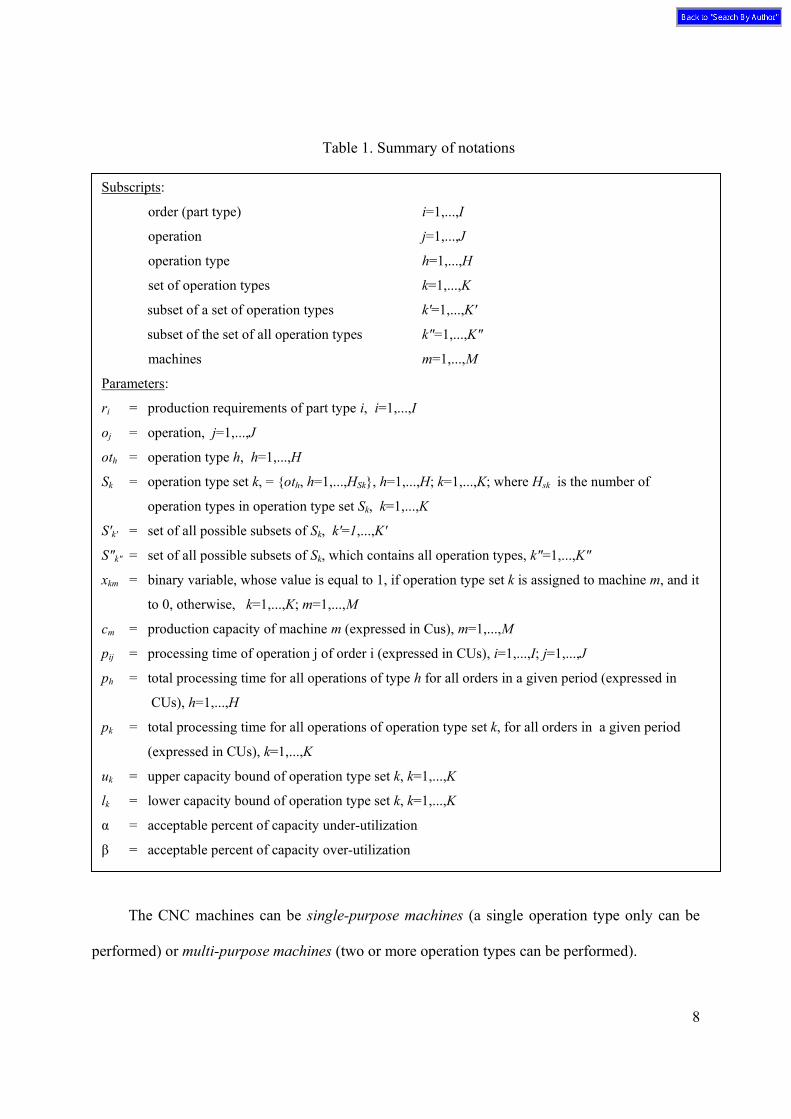
Table 1. Summary of notations

The CNC machines can be single-purpose machines (a single operation type only can be

performed) or multi-purpose machines (two or more operation types can be performed).

Subscripts:

order (part type) i=1,...,I

operation j=1,...,J

operation type h=1,...,H

set of operation types k=1,...,K

subset of a set of operation types k'=1,...,K'

subset of the set of all operation types k"=1,...,K"

machines m=1,...,M

Parameters:

ri = production requirements of part type i, i=1,...,I

oj = operation, j=1,...,J

oth = operation type h, h=1,...,H

Sk = operation type set k, = {oth, h=1,...,HSk}, h=1,...,H; k=1,...,K; where Hsk is the number of

operation types in operation type set Sk, k=1,...,K

S'k' = set of all possible subsets of Sk, k'=1,...,K'

S"k" = set of all possible subsets of Sk, which contains all operation types, k"=1,...,K"

xkm = binary variable, whose value is equal to 1, if operation type set k is assigned to machine m, and it

to 0, otherwise, k=1,...,K; m=1,...,M

cm = production capacity of machine m (expressed in Cus), m=1,...,M

pij = processing time of operation j of order i (expressed in CUs), i=1,...,I; j=1,...,J

ph = total processing time for all operations of type h for all orders in a given period (expressed in

CUs), h=1,...,H

pk = total processing time for all operations of operation type set k, for all orders in a given period

(expressed in CUs), k=1,...,K

uk = upper capacity bound of operation type set k, k=1,...,K

lk = lower capacity bound of operation type set k, k=1,...,K

α = acceptable percent of capacity under-utilization

β = acceptable percent of capacity over-utilization

9

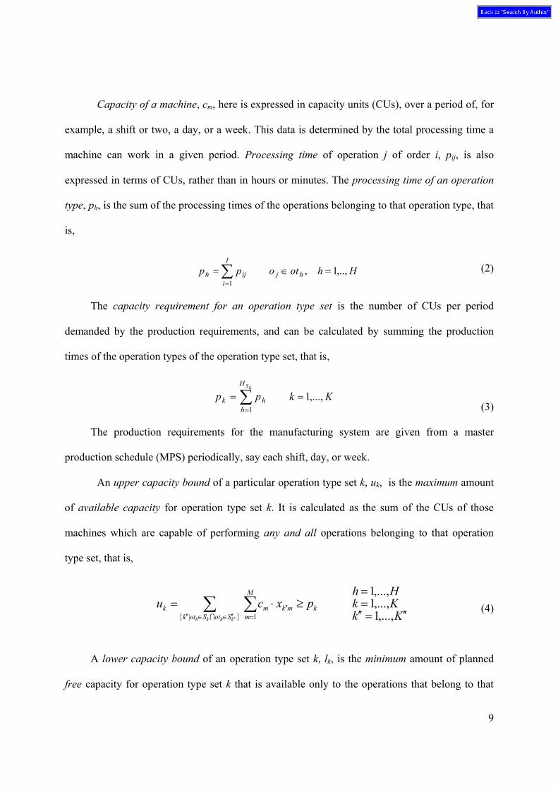
Capacity of a machine, cm, here is expressed in capacity units (CUs), over a period of, for

example, a shift or two, a day, or a week. This data is determined by the total processing time a

machine can work in a given period. Processing time of operation j of order i, pij, is also

expressed in terms of CUs, rather than in hours or minutes. The processing time of an operation

type, ph, is the sum of the processing times of the operations belonging to that operation type, that

is,

(2)

The capacity requirement for an operation type set is the number of CUs per period

demanded by the production requirements, and can be calculated by summing the production

times of the operation types of the operation type set, that is,

(3)

The production requirements for the manufacturing system are given from a master

production schedule (MPS) periodically, say each shift, day, or week.

An upper capacity bound of a particular operation type set k, uk, is the maximum amount

of available capacity for operation type set k. It is calculated as the sum of the CUs of those

machines which are capable of performing any and all operations belonging to that operation

type set, that is,

(4)

A lower capacity bound of an operation type set k, lk, is the minimum amount of planned

free capacity for operation type set k that is available only to the operations that belong to that

Hhotopp hj

I

iijh ,..,1,

1=∈=∑

=

KkppkSH

hhk ,...,1

1== ∑

=

{ } KkKkHh

pxcu kSotSotk

M

mmkmk

khkh ′′=′′==

≥⋅= ∑ ∑′′′′∈∈′′ =

′′,...,1

,...,1,...,1

| 1I

10

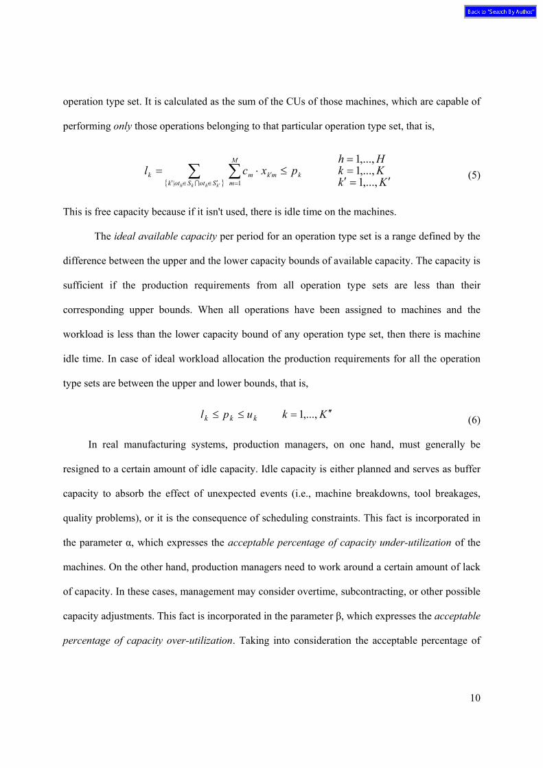
operation type set. It is calculated as the sum of the CUs of those machines, which are capable of

performing only those operations belonging to that particular operation type set, that is,

(5)

This is free capacity because if it isn't used, there is idle time on the machines.

The ideal available capacity per period for an operation type set is a range defined by the

difference between the upper and the lower capacity bounds of available capacity. The capacity is

sufficient if the production requirements from all operation type sets are less than their

corresponding upper bounds. When all operations have been assigned to machines and the

workload is less than the lower capacity bound of any operation type set, then there is machine

idle time. In case of ideal workload allocation the production requirements for all the operation

type sets are between the upper and lower bounds, that is,

(6)

In real manufacturing systems, production managers, on one hand, must generally be

resigned to a certain amount of idle capacity. Idle capacity is either planned and serves as buffer

capacity to absorb the effect of unexpected events (i.e., machine breakdowns, tool breakages,

quality problems), or it is the consequence of scheduling constraints. This fact is incorporated in

the parameter α, which expresses the acceptable percentage of capacity under-utilization of the

machines. On the other hand, production managers need to work around a certain amount of lack

of capacity. In these cases, management may consider overtime, subcontracting, or other possible

capacity adjustments. This fact is incorporated in the parameter β, which expresses the acceptable

percentage of capacity over-utilization. Taking into consideration the acceptable percentage of

{ } KkKkHh

pxcl kSotSotk

M

mmkmk

khkh ′=′==

≤⋅= ∑ ∑′′∈∈′ =

′,...,1,...,1,...,1

| 1I

Kkupl kkk ′′=≤≤ ,...,1

11

under-, and over-utilization, a more pragmatic condition for the production requirements is the

following,

(7)

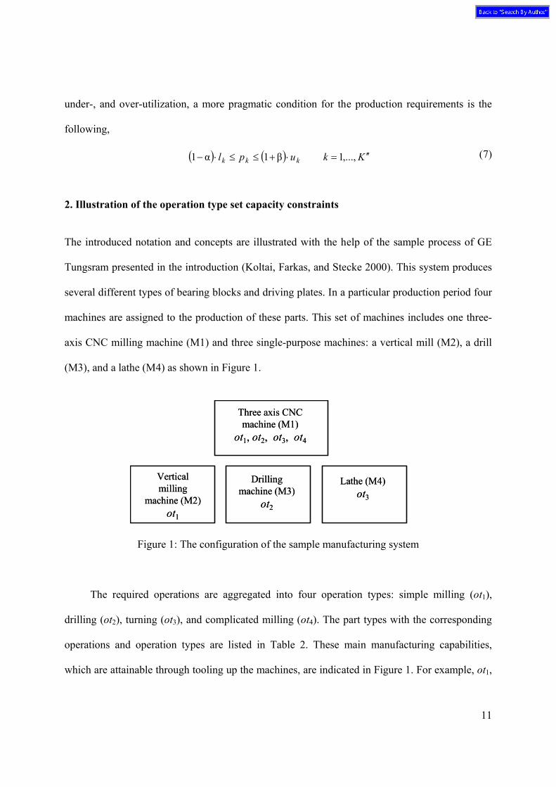
2. Illustration of the operation type set capacity constraints The introduced notation and concepts are illustrated with the help of the sample process of GE

Tungsram presented in the introduction (Koltai, Farkas, and Stecke 2000). This system produces

several different types of bearing blocks and driving plates. In a particular production period four

machines are assigned to the production of these parts. This set of machines includes one three-

axis CNC milling machine (M1) and three single-purpose machines: a vertical mill (M2), a drill

(M3), and a lathe (M4) as shown in Figure 1.

Figure 1: The configuration of the sample manufacturing system

The required operations are aggregated into four operation types: simple milling (ot1),

drilling (ot2), turning (ot3), and complicated milling (ot4). The part types with the corresponding

operations and operation types are listed in Table 2. These main manufacturing capabilities,

which are attainable through tooling up the machines, are indicated in Figure 1. For example, ot1,

Three axis CNC machine (M1)

ot1, ot2, ot3, ot4

Vertical milling

machine (M2)ot1

Lathe (M4)ot3

Drilling machine (M3)

ot2

Three axis CNC machine (M1)

ot1, ot2, ot3, ot4

Vertical milling

machine (M2)ot1

Lathe (M4)ot3

Drilling machine (M3)

ot2

( ) ( ) Kkupl kkk ′′=⋅+≤≤⋅− ,...,111 βα

12

ot2, ot3, and ot4 at machine M1 indicates that M1 is capable of performing all the operation types,

whereas M2, M3, and M4, respectively, are single-purpose machines for ot1, ot2, and ot3.

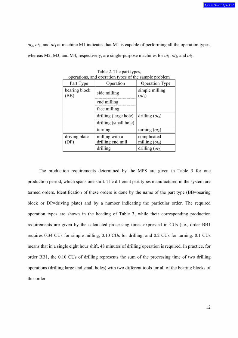
Table 2. The part types,

operations, and operation types of the sample problem Part Type Operation Operation Type

bearing block (BB) side milling simple milling

(ot1) end milling face milling drilling (large hole) drilling (ot2) drilling (small hole) turning turning (ot3) driving plate (DP)

milling with a drilling end mill

complicated milling (ot4)

drilling drilling (ot2)

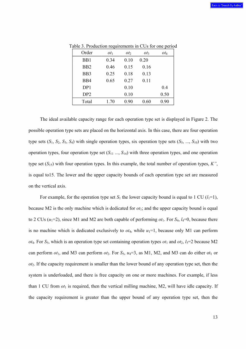
The production requirements determined by the MPS are given in Table 3 for one

production period, which spans one shift. The different part types manufactured in the system are

termed orders. Identification of these orders is done by the name of the part type (BB=bearing

block or DP=driving plate) and by a number indicating the particular order. The required

operation types are shown in the heading of Table 3, while their corresponding production

requirements are given by the calculated processing times expressed in CUs (i.e., order BB1

requires 0.34 CUs for simple milling, 0.10 CUs for drilling, and 0.2 CUs for turning. 0.1 CUs

means that in a single eight hour shift, 48 minutes of drilling operation is required. In practice, for

order BB1, the 0.10 CUs of drilling represents the sum of the processing time of two drilling

operations (drilling large and small holes) with two different tools for all of the bearing blocks of

this order.

13

Table 3. Production requirements in CUs for one period Order ot1 ot2 ot3 ot4 BB1 0.34 0.10 0.20 BB2 0.46 0.15 0.16 BB3 0.25 0.18 0.13 BB4 0.65 0.27 0.11 DP1 0.10 0.4 DP2 0.10 0.50 Total 1.70 0.90 0.60 0.90

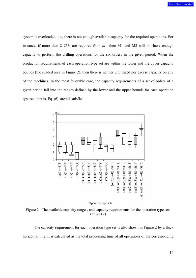
The ideal available capacity range for each operation type set is displayed in Figure 2. The

possible operation type sets are placed on the horizontal axis. In this case, there are four operation

type sets (S1, S2, S3, S4) with single operation types, six operation type sets (S5, ..., S10) with two

operation types, four operation type set (S11 ..., S14) with three operation types, and one operation

type set (S15) with four operation types. In this example, the total number of operation types, K”,

is equal to15. The lower and the upper capacity bounds of each operation type set are measured

on the vertical axis.

For example, for the operation type set S1 the lower capacity bound is equal to 1 CU (l1=1),

because M2 is the only machine which is dedicated for ot1; and the upper capacity bound is equal

to 2 CUs (u1=2), since M1 and M2 are both capable of performing ot1. For S4, l4=0, because there

is no machine which is dedicated exclusively to ot4, while u1=1, because only M1 can perform

ot4. For S5, which is an operation type set containing operation types ot1 and ot2, l5=2 because M2

can perform ot1, and M3 can perform ot2. For S5, u4=3, as M1, M2, and M3 can do either ot1 or

ot2. If the capacity requirement is smaller than the lower bound of any operation type set, then the

system is underloaded, and there is free capacity on one or more machines. For example, if less

than 1 CU from ot1 is required, then the vertical milling machine, M2, will have idle capacity. If

the capacity requirement is greater than the upper bound of any operation type set, then the

14

system is overloaded, i.e., there is not enough available capacity for the required operations. For

instance, if more than 2 CUs are required from ot1, then M1 and M2 will not have enough

capacity to perform the drilling operations for the six orders in the given period. When the

production requirements of each operation type set are within the lower and the upper capacity

bounds (the shaded area in Figure 2), then there is neither unutilized nor excess capacity on any

of the machines. In the most favorable case, the capacity requirements of a set of orders of a

given period fall into the ranges defined by the lower and the upper bounds for each operation

type set, that is, Eq. (6). are all satisfied.

Figure 2.: The available capacity ranges, and capacity requirements for the operation type sets (α=β=0.2)

The capacity requirement for each operation type set is also shown in Figure 2 by a thick

horizontal line. It is calculated as the total processing time of all operations of the corresponding

0

1

2

3

4

5

6

{ot(1

)}=S

(1)

{ot(2

)}=S

(2)

{ot(3

)}=S

(3)

{ot(4

)}=S

(4)

{ot(1

);ot(2

)}=S

(5)

{ot(1

);ot(3

)}=S

(6)

{ot(1

);ot(4

)}=S

(7)

{ot(2

);ot(3

)}=S

(8)

{ot(2

);ot(4

)}=S

(9)

{ot(3

);ot(4

)}=S

(10)

{ot(1

);ot(2

);ot(3

)}=S

(11)

{ot(1

);ot(2

);ot(4

)}=S

(12)

{ot(2

);ot(3

);ot(4

)}=S

(13)

{ot(1

);ot(3

);ot(4

)}=S

(14)

{ot(1

);ot(2

);ot(3

);ot(4

)}=S

(15)

Operation type sets

[CU]

15

operation type set. For example, the processing time for operation type set S1 is equal to 1.7 CUs,

because this operation type set contains only ot1, while the processing time for operation type set

S5 is equal to 2.6 CUs, which is the sum of the total processing time of ot1, and ot2 (see Eq. (3).).

Figure 2 can be used to determine whether or not the manufacturing system is in complete

technological balance, i.e., to check whether there is any excess capacity or lack of capacity from

certain operation types. In our case, Figure 2 shows that there are under-loadings at S2, S3, and S8.

The under-loading at S2 indicates that if all drilling operations are processed on M3, then this

machine still has idle capacity. The under-loading at S3 indicates the same fact for turning, that is,

if all turning operations are processed on M4, then this machine still has idle capacity. The under-

loading of S8 points out that the system has more drilling and turning capacity than necessary.

Figure 2 shows over-loadings in S7, S12, S14, and S15. The over-loading at S7 indicates that

the total capacity requirements of ot1 and ot4 are higher than the total available capacity on M1

and on M2. The over-loading at S12 indicates that the capacity requirement of ot1, ot2, and ot4

together are higher than the available capacities on machines M1, M2, and M3. Therefore, even if

we do not assign any operations belonging to ot2 to M1, we still do not have enough capacity for

the operation types ot1, and ot2. The meaning of the over- loading of S14 is similar to the over-

loading of S12. It indicates that the capacity requirements of ot1, ot3, and ot4 together are higher,

than the available capacities on machines M1, M2, and M4. Therefore, even if we do not assign

any operations belonging to ot3 to M1, we still do not have enough capacity for the operation

types ot1, and ot2. The consequence of these two over-loadings is that it is unnecessary to tool M4

for all of the operations, because the production requirements for the operation types ot1 and ot4 is

so high that we will not be able to utilize the operational flexibility, that M1 offers. Finally, the

over-loading at S15 means that the capacity requirements of all of the operation types are higher

than the available capacities of all of the machines.

16

In summary, on the one hand there could be idle capacity on certain machines, while there

might not be enough capacity to fulfill all of the requirements for certain operation types. Figure

2 also displays the increased ideal capacity range when 20 percent capacity over- and under-

utilization are acceptable for the management (α=β=0.2). The thin lines extending from the top

and the bottom of the shaded boxes represent the increased upper bounds and the decreased lower

bounds. The capacity requirements are within this extended range for most of the operation type

sets. For S3, however, the production requirement is below the decreased capacity lower bound,

therefore M3 will be unacceptably under-utilized. This problem can be solved by several ways,

such as adding a new order to the existing six orders, exchanging an existing order with one with

higher production requirement for ot3 or, changing the capacity of the machine (reducing its

working time), etc. In our case this would solve the problem at S8 as well, where the production

requirement is also outside the acceptable capacity range. For S7 the problem is just the opposite,

the production requirement is higher than the increased capacity upper bound. There is not

enough capacity to perform all of the operations of ot1 and ot4. This problem can be solved by

several ways, such as removing an order from the existing six orders by scheduling it for a later

period, exchanging an existing order with one with less production requirements for ot1 and ot4,

scheduling extra overtime, etc.

3. Sensitivity analysis of the available capacity

Sensitivity analyses of the parameters of the model can help to analyze how certain changes

affect the capacity over- and under-utilization of the manufacturing system. The production

requirements (ph) of an operation type and the machine capacity (cm) are the most important

parameters altered by unexpected changes. For these instances, sensitivity analysis can determine

the validity range of a chosen parameter within which the system remains balanced, that is, the

17

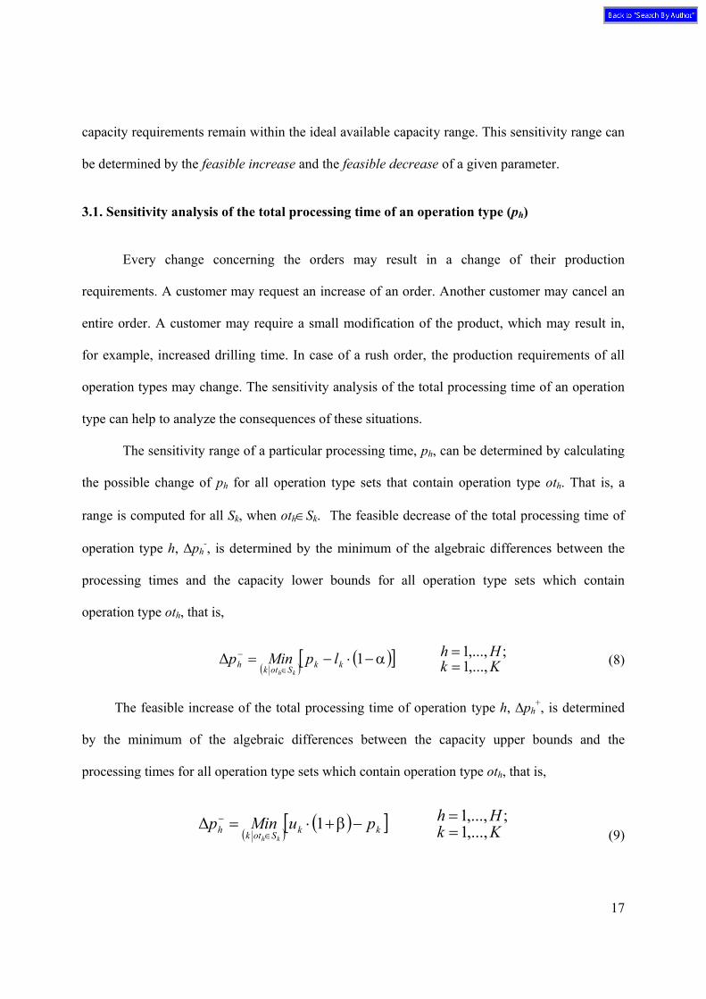
capacity requirements remain within the ideal available capacity range. This sensitivity range can

be determined by the feasible increase and the feasible decrease of a given parameter.

3.1. Sensitivity analysis of the total processing time of an operation type (ph) Every change concerning the orders may result in a change of their production

requirements. A customer may request an increase of an order. Another customer may cancel an

entire order. A customer may require a small modification of the product, which may result in,

for example, increased drilling time. In case of a rush order, the production requirements of all

operation types may change. The sensitivity analysis of the total processing time of an operation

type can help to analyze the consequences of these situations.

The sensitivity range of a particular processing time, ph, can be determined by calculating

the possible change of ph for all operation type sets that contain operation type oth. That is, a

range is computed for all Sk, when oth∈Sk. The feasible decrease of the total processing time of

operation type h, ∆ph-, is determined by the minimum of the algebraic differences between the

processing times and the capacity lower bounds for all operation type sets which contain

operation type oth, that is,

(8)

The feasible increase of the total processing time of operation type h, ∆ph+, is determined

by the minimum of the algebraic differences between the capacity upper bounds and the

processing times for all operation type sets which contain operation type oth, that is,

(9)

( )( )[ ] Kk

HhlpMinp kkSotkhkh ,...,1

;,...,11 ==α−⋅−=

∈

−∆

( )( )[ ] Kk

HhpuMinp kkSotkhkh ,...,1

;,...,11 ==−β+⋅=

∈

−∆

18

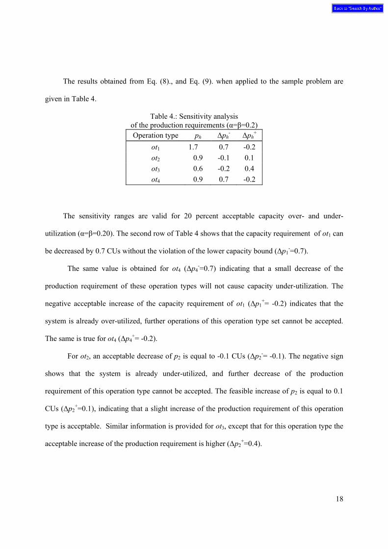
The results obtained from Eq. (8)., and Eq. (9). when applied to the sample problem are

given in Table 4.

Table 4.: Sensitivity analysis of the production requirements (α=β=0.2) Operation type ph ∆ph

- ∆ph+

ot1 1.7 0.7 -0.2 ot2 0.9 -0.1 0.1 ot3 0.6 -0.2 0.4 ot4 0.9 0.7 -0.2

The sensitivity ranges are valid for 20 percent acceptable capacity over- and under-

utilization (α=β=0.20). The second row of Table 4 shows that the capacity requirement of ot1 can

be decreased by 0.7 CUs without the violation of the lower capacity bound (∆p1-=0.7).

The same value is obtained for ot4 (∆p4-=0.7) indicating that a small decrease of the

production requirement of these operation types will not cause capacity under-utilization. The

negative acceptable increase of the capacity requirement of ot1 (∆p1+= -0.2) indicates that the

system is already over-utilized, further operations of this operation type set cannot be accepted.

The same is true for ot4 (∆p4+= -0.2).

For ot2, an acceptable decrease of p2 is equal to -0.1 CUs (∆p2-= -0.1). The negative sign

shows that the system is already under-utilized, and further decrease of the production

requirement of this operation type cannot be accepted. The feasible increase of p2 is equal to 0.1

CUs (∆p2+=0.1), indicating that a slight increase of the production requirement of this operation

type is acceptable. Similar information is provided for ot3, except that for this operation type the

acceptable increase of the production requirement is higher (∆p2+=0.4).

19

The results in Table 4 are independent validity ranges, that is, the feasible decrease and

increase is valid only if the capacity requirements of a single operation type change. When the

capacity requirements of more than one operation type set changes, a joint range for all of the

simultaneously changing parameters can be determined.

3.2. Sensitivity analysis of the machine capacity (cm) The capacity of the machines may decrease because of machine breakdowns, unexpected

production stops, or waiting for operators, repair-persons, or tools and materials. A capacity

increase can be regarded as scheduled overtime or as the organization of extra shifts. Sensitivity

analysis of the machine capacity can help analyze these situations.

The sensitivity range of the available capacity of a particular machine can be determined

by calculating the feasible change of the upper and lower capacity bounds of all of those

operation type sets which are affected by the change of the operation type set assigned to that

machine. For example, if a machine is tooled just for drilling, then the feasible change of the

upper and lower capacity bounds of all of those operation type sets which contains drilling has to

be examined.

The capacity decrease of a machine diminishes both the lower and upper capacity bounds.

For our purposes, the decrease of the upper bound is relevant, because it may result in an

infeasible capacity over-utilization. When the capacity of a particular machine changes, then all

of the capacity upper bounds of those operation type sets, which contain any and all of the

operation types assigned to this machine, are affected. The feasible decrease of the capacity of

machine m, ∆cm-, is determined by the minimum of the algebraic differences between the

capacity upper bound and the processing time for all of the affected operation type sets, that is,

20

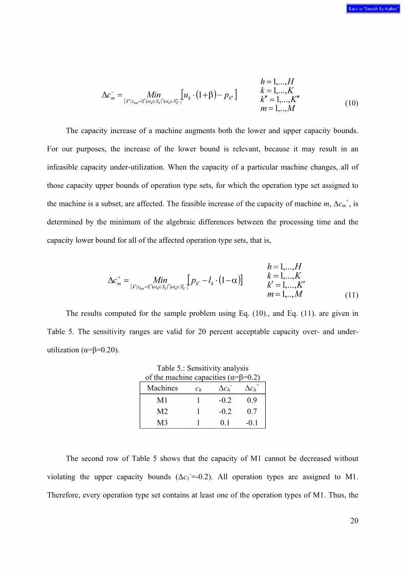
(10)

The capacity increase of a machine augments both the lower and upper capacity bounds.

For our purposes, the increase of the lower bound is relevant, because it may result in an

infeasible capacity under-utilization. When the capacity of a particular machine changes, all of

those capacity upper bounds of operation type sets, for which the operation type set assigned to

the machine is a subset, are affected. The feasible increase of the capacity of machine m, ∆cm+, is

determined by the minimum of the algebraic differences between the processing time and the

capacity lower bound for all of the affected operation type sets, that is,

(11)

The results computed for the sample problem using Eq. (10)., and Eq. (11). are given in

Table 5. The sensitivity ranges are valid for 20 percent acceptable capacity over- and under-

utilization (α=β=0.20).

Table 5.: Sensitivity analysis of the machine capacities (α=β=0.2) Machines ch ∆ch

- ∆ch+

M1 1 -0.2 0.9 M2 1 -0.2 0.7 M3 1 0.1 -0.1

The second row of Table 5 shows that the capacity of M1 cannot be decreased without

violating the upper capacity bounds (∆c1-=-0.2). All operation types are assigned to M1.

Therefore, every operation type set contains at least one of the operation types of M1. Thus, the

{ }( )[ ]

MmKk

KkHh

puMinc kkSotSotxkmkhkhkm

,..,1,...,1

,...,1,...,1

11|

=′′=′′

==

−β+⋅= ′′′′∈∈=′′

−

′′II∆

{ }( )[ ]

MmKkKkHh

lpMinc kkSotSotxkmkhkhkm

,..,1,...,1,...,1,...,1

11|

=′=′

==

α−⋅−= ′′∈∈=′

+

′II∆

21

difference between the 20 percent increased value of the upper bounds and the capacity

requirements for all operation type sets must be checked, and the minimum of Eq. (10) is found

at S7. Figure 2 shows that for S7, the capacity requirement is higher than the acceptable capacity

over-utilization. Therefore, the capacities of those machines, which contain ot1 and ot4 cannot be

decreased. This also explains the negative value found for the feasible decrease of the capacity of

M2 (∆c2-= -0.2). The feasible increase of the capacity of M1 is equal to 0.9 (∆c1

+=0.9). The

operation type set assigned to M1 is S15. This is the largest set and it affects exclusively the lower

capacity bound of operation type set S15. (S15 is a subset of only itself.) Thus, the difference

between the capacity requirements and the 20 percent decreased values of the lower bounds must

be checked at S15 and it is equal to 0.9 CUs. For M2, the assigned S1 is a subset of eight operation

type sets. The smallest difference between the capacity requirements and the 20 percent

decreased value of the lower bounds is found at S6, and is equal to 0.7 (∆c2+=0.7).

Machine M3 contains a single operation type, ot2. In this case, the feasible decrease of the

machine capacity is equivalent to the feasible increase of the production requirements of ot2, that

is, ∆c3-=∆p2

+=0.1. Similarly, the feasible increase of the machine capacity is equivalent to the

feasible decrease of the production requirements of ot2, that is, ∆c3+=∆p2

-=-0.1. Machine M4

also contains a single operation type, ot3. The last row of Table 5 shows that the feasible capacity

change of this machine is the same as the feasible change of the production requirements of ot3,

except that the value of the feasible decrease must be changed by the value of the feasible

increase.

4. Conclusions FMSs are capable of performing a wide variety of technologically different operations.

Therefore, any model trying to handle all of the operations has to cope with the problem of

22

complexity. The aggregation of operations into operation types can help to address this problem.

The presented method provides an easy to use tool to analyze the availability of capacity. We

suggest two main areas for applying this concept.

1. Formulation of capacity constraints for aggregate production planning. Based on the

presented approach instead of the capacity of the machine the capacity of the operation types can

be formulated. This has major advantages, when just a quick, overall estimation of the available

capacity is required. When the operations manager would like to estimate whether the available

capacity of a flexible system is enough for the manufacturing of a set of orders, then it is not

necessary to determine the detailed production plan containing route, and machine assignment. In

this case the operation type based formulation of capacity constraints can quickly provide the

answer (Koltai 2004).

2. On-line capacity analysis. The presented model provides an overview of the available

capacity when a set of orders is assigned to the system. For example, when a new order arrives,

the model can help check whether there is enough capacity to process it. If the arrival of the new

order results in excess production requirements for any operation type set, then a reschedule of

the new, or an existing order with lower priority, or retooling of machines, or capacity extensions

by overtime, etc., can be considered. In other cases, operation type sensitivity results (like Table

4.) show which operation types are in shortage and which is in excess, helping by this way the

production manager to improve capacity utilization by attracting new orders. Machine sensitivity

information (like Table 5) show which machines are critical from the point of view of completing

the orders in time.

3. Machine tooling. For a particular set of orders, a machine tooling can be determined,

which provides acceptable balance, that is, the production requirements of the operation type sets

are within the ideal capacity range. A model is provided by Koltai et al. (2004) which determines

23

acceptably balanced systems for a set of orders considering several management priorities, such

as tooling cost, machine pooling, flexibility, etc.

The major complexity of the capacity analysis of flexible manufacturing systems is

caused by the possibility of alternative use of the machines. The presented methods provide an

aggregate view about the available capacity, considering the operations requirement of the parts

and the manufacturing capabilities of the system. The model is based on the traditional

aggregation concept of production planning. In a flexible environment, however, the operation is

recommended for aggregation. Applying this concept, several production planning and control

models can be developed to help the production manager in decision-making.

ACKNOWLEDGMENTS

The research was supported by the Hungarian National Foundation for Scientific

Research, Grant Number OTKA T034110

REFERENCES

Hax, A. C., and Candea, C.: Production and Inventory Management, Prentice-Hall,

Englewood Cliffs, NJ. 1984.

Holt, C. C., Modigliani, F., Muth, J. F., and Simon, H. A.: Planning Production,

Inventories and Work Force, Prentice-Hall, Englewood Cliffs, NJ, 1960.

Jaikumar, R., and van Wassenhove, L.,N.: A Production Planning Framework for Flexible

Manufacturing Systems, Journal of Manufacturing and Operations Management, Vol. 2, pp. 52-

79, 1989.

Johnson, L. A., and Montgomery, D. C.: Operations Research in Production Planning,

Scheduling and Inventory Control, John Wiley and Sons, NY, 1974.

24

Koltai, T., Stecke, K. E., and Juhász V.: Planning of Flexibility of Flexible Manufacturing

Systems, In: Proceedings of 2004 JUSFA, 2004 Japan – USA Symposium on Flexible

Automation. (Accepted for publication)

Koltai, T., Stecke, K. E., and Juhász V.: A New Formulation of Capacity Constraints in

the Production Planning of Flexible Manufacturing Systems, In: Proceedings of FAIM 2004,

Conference of Flexible Automation and Intelligent Manufacturing. (Accepted for publication)

Koltai T., Farkas, A., Stecke, K.: An aggregate capacity analysis model for a flexible

manufacturing environment. 2000 Japan-USA Symposium on Flexible Automation, Ann Arbor,

MI, ASME International, pp. 1-8, 2000,

Koltai, T., Farkas, F., and Stecke, K. E.: Aggregate Production Planning of Flexible

Manufacturing Systems Using the Concept of Operation Types, Working Paper #98-007,

University of Michigan Business School, Ann Arbor, Michigan 1998.

Mazzola, J.B., Neebe, A.W., And Dunn, C.V.R.: Multiproduct Production Planning in the

Presence of Work-Force Learning, European Journal of Operational Research, 106, 2-3, 336-

356, 1998.

Niess, P. S.: Kapacitätsabgleich bei Flexiblen Fertigungssytemen, IPA Forschung und

Praxis, Springer Verlag, Berlin, Germany, 1980.

Stecke, K. E.: Formulation and Solution of Nonlinear Integer Production Planning

Problems for Flexible Manufacturing Systems, Management Science, Vol. 29, No. 3, pp. 273-

288, 1983.

Stecke, K. E.: A Hierarchical Approach to Solving Machine Grouping and Loading

Problems of Flexible Manufacturing Systems, European Journal of Operational Research, Vol.

24, pp. 369-378, 1986.

25

Stecke, K. E., and Kim, I.: A Flexible Approach to Part Type Selection in Flexible Flow

Systems Using Part Mix Ratios, International Journal of Production Research, Vol. 29, No.1, pp.

53-75, 1991.

Thomas, L. J., and McClain, J. O.: An Overview of Production Planning, In: Logistics of

Production and Inventory (Editors, Graves, S. C., Rinnooy Kan, A. H. G., and Zipkin, P. H.),

North-Holland, Amsterdam, The Netherlands, 1993.

Van Looveren, A. J., Gelders, L. F., and van Wassenhove, L. N.: A Review of FMS

Planning Models, In: Modeling and Design of Flexible Manufacturing Systems, (Editor, Kusiak,

A.), Elseviers Science Publishers B.V., Amsterdam, The Netherlands, pp. 3-31, 1986.