ABSTRACT

MARATHE, JAYDEEP P. METRIC: Tracking Memory Bottlenecks via Binary Rewriting

(Under the direction of Assistant Professor Dr. Frank Mueller).

Over recent decades, computing speeds have grown much faster than memory ac-

cess speeds. This differential rate of improvement between processor speeds and memory

speeds has led to an ever-increasing processor-memory gap. Overall computing speeds for

for most applications are now dominated by the cost of their memory references. Further-

more, memory access costs will grow increasingly dominant as the processor-memory gap

widens. In this scenario, characterizing and quantifying application program memory usage

to isolate, identify and eliminate memory access bottlenecks will have significant impact on

overall application computing performance.

This thesis presentsMETRIC, an environment for determining memory access inef-

ficiencies by examining access traces. This thesis makes three primary contributions. First,

we present methods to extract partial access traces from running applications by observing

their memory behavior via dynamic binary rewriting. Second, we present a methodology to

represent partial access traces in constant space for regular references through a novel tech-

nique for online compression of reference streams. Third, we employ offline cache simulation

to derive indications about memory performance bottlenecks from partial access traces. By

examining summarized and by-reference metrics as well as cache evictor information, we

can pinpoint the sources of performance problems. We perform validation experiments of

the framework with respect to accuracy, compression and execution overheads for several

benchmarks. Finally, we demonstrate the ability to derive opportunities for optimizations

and assess their benefits in several case studies, resulting in up to 40% lower miss ratios.

METRIC: Tracking Memory Bottlenecks via Binary Rewriting

by

Jaydeep P. Marathe

A thesis submitted to the Graduate Faculty of

North Carolina State University

in partial satisfaction of the

requirements for the Degree of

Master of Science in Computer Science

Department of Computer Science

Raleigh

2003

Approved By:

Dr. Vincent Freeh Dr. Gregory Byrd

Dr. Frank MuellerChair of Advisory Committee

ii

Biography

Jaydeep Marathe was born on 28th November 1978, in Pune, India. He received

his Bachelor of Engineering in Computer Engineering from the University of Pune, India,

in 2000. He worked with Pace Soft-Silicon Ltd. as a Software Engineer for a year, before

starting graduate studies at the North Carolina State University. With the defense of this

thesis, he is receiving the Master of Science in Computer Science degree from NCSU, in

July 2003.

iii

Acknowledgements

I would like to thank Dr. Frank Mueller for his guidance and support during

the duration of this project, and especially his insistence on consistent writing and coding

styles. I would also like to thank Dr. Vincent Freeh and Dr. Gregory Byrd for being on

my advisory committee.

iv

Contents

List of Figures vi

1 Introduction 11.1 Conventional Profiling Approaches . . . . . . . . . . . . . . . . . . . . . . . 1

1.1.1 Gprof . . . . . . . . . . . . . . . . . . . . . . . . . . . . . . . . . . . 21.1.2 Hardware Performance Counters . . . . . . . . . . . . . . . . . . . . 21.1.3 Incremental Memory Hierarchy Simulation . . . . . . . . . . . . . . 4

1.2 Motivation and Approach . . . . . . . . . . . . . . . . . . . . . . . . . . . . 51.2.1 METRIC . . . . . . . . . . . . . . . . . . . . . . . . . . . . . . . . . 51.2.2 Dynamic Binary Rewriting vs. Static Instrumentation . . . . . . . . 61.2.3 Partial vs. Complete Traces . . . . . . . . . . . . . . . . . . . . . . . 6

1.3 Outline . . . . . . . . . . . . . . . . . . . . . . . . . . . . . . . . . . . . . . 7

2 The METRIC Framework 82.1 Dynamic Binary Rewriting . . . . . . . . . . . . . . . . . . . . . . . . . . . 82.2 Framework Overview . . . . . . . . . . . . . . . . . . . . . . . . . . . . . . . 9

2.2.1 Target Instrumentation . . . . . . . . . . . . . . . . . . . . . . . . . 112.2.2 Trace Generation and Compression . . . . . . . . . . . . . . . . . . . 11

2.3 Online Detection of Access Patterns . . . . . . . . . . . . . . . . . . . . . . 142.3.1 Space Complexity . . . . . . . . . . . . . . . . . . . . . . . . . . . . 202.3.2 Time Complexity . . . . . . . . . . . . . . . . . . . . . . . . . . . . . 202.3.3 Comparison with Previous Work . . . . . . . . . . . . . . . . . . . . 22

2.4 Cache Simulation and User Feedback . . . . . . . . . . . . . . . . . . . . . . 22

3 Case Studies 263.0.1 Case Study: Matrix Multiplication (mm) . . . . . . . . . . . . . . . 263.0.2 Case Study: Erlebacher ADI Integration . . . . . . . . . . . . . . . . 32

4 Validation Experiments 364.1 Experiment 1. Accuracy of Simulation . . . . . . . . . . . . . . . . . . . . . 364.2 Experiment 2. Compression Rate . . . . . . . . . . . . . . . . . . . . . . . . 374.3 Experiment 3. Execution Overhead . . . . . . . . . . . . . . . . . . . . . . . 38

5 Related Work 41

v

6 Conclusions and Future Work 44

Bibliography 46

vi

List of Figures

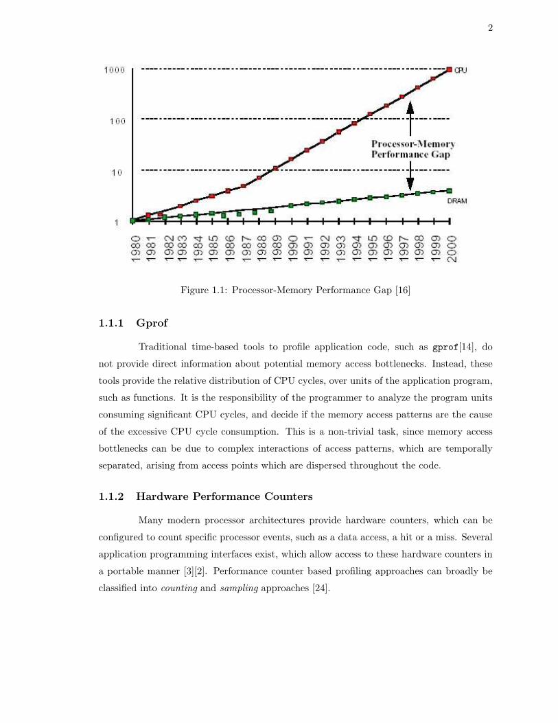
1.1 Processor-Memory Performance Gap [16] . . . . . . . . . . . . . . . . . . . . 21.2 3 Stages for Trace-based Simulators [29] . . . . . . . . . . . . . . . . . . . . 4

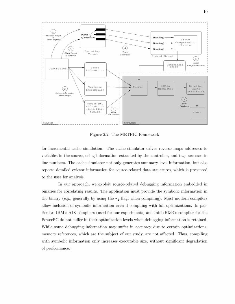
2.1 Inserting Instrumentation at a Point . . . . . . . . . . . . . . . . . . . . . . 92.2 The METRIC Framework . . . . . . . . . . . . . . . . . . . . . . . . . . . . 102.3 Example: Representing Regular Access Patterns . . . . . . . . . . . . . . . 122.4 PRSD Representation . . . . . . . . . . . . . . . . . . . . . . . . . . . . . . 152.5 Flowchart: Processing at each Level . . . . . . . . . . . . . . . . . . . . . . 162.6 Semantics of is compatible sibling & is compatible child . . . . . . . . . . . 172.7 Illustration of the Compression Algorithm . . . . . . . . . . . . . . . . . . . 182.8 (Continued)Illustration of the Compression Algorithm . . . . . . . . . . . . 192.9 A Comparison of Our Algorithm with Previous Work . . . . . . . . . . . . . 25

3.1 Per-Reference Cache Statistics for Unoptimized Matrix Multiply . . . . . . 273.2 Evictor Information for Unoptimized Matrix Multiply . . . . . . . . . . . . 273.3 Per-Reference Cache Statistics for Optimized Matrix Multiply . . . . . . . . 283.4 Evictor Information for Optimized Matrix Multiply . . . . . . . . . . . . . . 293.5 Contrasted Metrics for Matrix Multiply before and after Optimizations . . 313.6 Contrasted Metrics for ADI before and after Optimizations . . . . . . . . . 33

4.1 Comparison of load misses reported by HPM and Cache Simulator . . . . . 374.2 Potential Causes of Cache Interference . . . . . . . . . . . . . . . . . . . . . 384.3 Comparison of uncompressed and compressed trace sizes . . . . . . . . . . . 394.4 Execution Overhead in Target Execution . . . . . . . . . . . . . . . . . . . . 40

1

Chapter 1

Introduction

Over recent decades, computing speeds have grown much faster than memory

access speeds. Figure 1.1 shows that while micro-processor performance has been improving

at a rate of 60% per year, the access time to DRAM has been improving at less than 10% per

year [16][27]. This differential rate of improvement between processor speeds and memory

speeds has led to an ever-increasing processor-memory gap. Memory hierarchies have been

introduced to combat this gap; however, overall computing speeds for most applications are

still dominated by the cost of their memory references. Furthermore, memory access costs

will grow increasingly dominant as the processor-memory gap widens.

In this scenario, characterizing and quantifying application program memory us-

age to isolate, identify and eliminate memory access bottlenecks will have significant impact

on overall application computing performance. This thesis discusses the design, implemen-

tation and validation of such a memory profiling tool.

1.1 Conventional Profiling Approaches

This section discusses conventional approaches to profiling memory hierarchy us-

age. We elucidate three broad approaches to the problem, each providing increasingly

detailed information about memory hierarchy usage, however with a corresponding increase

in the computing and stable storage overheads.

2

Figure 1.1: Processor-Memory Performance Gap [16]

1.1.1 Gprof

Traditional time-based tools to profile application code, such as gprof[14], do

not provide direct information about potential memory access bottlenecks. Instead, these

tools provide the relative distribution of CPU cycles, over units of the application program,

such as functions. It is the responsibility of the programmer to analyze the program units

consuming significant CPU cycles, and decide if the memory access patterns are the cause

of the excessive CPU cycle consumption. This is a non-trivial task, since memory access

bottlenecks can be due to complex interactions of access patterns, which are temporally

separated, arising from access points which are dispersed throughout the code.

1.1.2 Hardware Performance Counters

Many modern processor architectures provide hardware counters, which can be

configured to count specific processor events, such as a data access, a hit or a miss. Several

application programming interfaces exist, which allow access to these hardware counters in

a portable manner [3][2]. Performance counter based profiling approaches can broadly be

classified into counting and sampling approaches [24].

3

In the counting approach, performance metrics are aggregated for specific regions

of the target application source code. Calls to start and stop performance counters are

placed selectively around interesting sections of the target application, such as program

functions or loop nests. As the application runs, the collected counter values are mapped to

the specific program code region being profiled and can also be aggregated to get an overall

performance report for the application. This approach requires modifying and recompiling

the target application to insert calls to the counter control routines. Calls are placed

manually or are inserted automatically by the compiler.

In the sampling approach, an “observer” process samples the hardware counters

at regular intervals. The observer process can be triggered periodically by a high resolution

timer interrupt, or by interrupt on counter overflow, for supporting architectures. An

interesting approach [5] uses an n-way search to increase the resolution of sampling. Initially,

the entire address range is profiled for cache miss events, using interrupt on counter overflow.

Subsequently, different hardware counters are assigned to specific address ranges that show

increased rate of misses, thereby identifying memory access bottlenecks. However, this

approach requires several advanced hardware features, such as support for partitioning the

address space over available counters, which are not widely available in current processor

architectures (except the Itanium [10]).

There are several problems with using hardware performance counters to track

performance bottlenecks. In the case of memory bottlenecks, the fundamental problem is

the coarse nature of the statistics, i.e., counter information is useful in highlighting the

symptoms of memory bottlenecks, but contains insufficient information to diagnose the

cause. It is left to the programmer to look at the apposite source code fragment and figure

out the cause of the bottleneck.

Additionally, in the sampling mode, there is a trade-off between the accuracy of

the samples and the rate of sampling. However, an excessive sampling rate can also perturb

the target application execution, e.g., by cache pollution, thereby affecting the accuracy of

results [24]. Furthermore, most hardware architectures have restrictions on the potential

events which can be tracked simultaneously, e.g., data cache loads and stores, and it may

require multiple runs of the application for different events to get a complete performance

breakdown.

4

1.1.3 Incremental Memory Hierarchy Simulation

Workload

Host Workstation

Trace CollectionTrace quality defined by:

CompletenessDistortionDetail

TimeTimeTime

WordByte

HalfWord

0x004b33000x00f5a4f00x00fb450c

Trace Reduction

Ideal Trace Reduction:10x to 100x Reduction FactorHigh SpeedNo Resulting Simulation Error

StorageSecondary

Trace Processing

Simulation Parameters:I−cache,D−cache,TLBSize, Line Size, AssociativityRandom, FIFO, LRU replacement

Metrics:

Miss Ratios

Temporal & Spatial RatiosSpatial Use

Figure 1.2: 3 Stages for Trace-based Simulators [29]

Memory hierarchy simulators provide a detailed view of a target application’s

memory hierarchy usage. These simulators use the address trace generated by the target

application to do incremental simulation. A comprehensive survey of trace based simulators

is presented in Uhlig et al. [29]. Figure 1.2 shows the typical stages for these tools - Trace

Collection, Trace Reduction and Trace Processing. Detailed access traces can be extracted

at virtually all system levels - from the circuit and microcode level, to the compiler and

operating system level [29]. The extracted address traces are relatively large, and they must

be effectively compressed for storing on a non-volatile medium, such as the hard disk (trace

reduction). Finally, the trace data is used for incremental memory hierarchy simulation.

Simulation using address traces has several advantages. Simulations are repeatable

and allow cache parameters and data layouts to be varied without regenerating the trace

data. They do not require hardware monitoring and access to or the existence of the machine

5

being studied. Most importantly, simulation usually takes place offline, i.e., on a separate

machine or process, and can therefore afford to maintain more detailed statistics, such as

correlation of memory events to source code lines and data structures [23].

However, increased accuracy and level of detail comes at a price. Modern proces-

sors are capable of generating gigabytes of data per second, especially on memory intensive

applications. Logging the complete access trace to stable storage causes significant degra-

dation in the computing speed of the target application, especially since trace collection has

to be done online. Storing complete address traces is also problematic, due to the large size

of the trace, even with trace reduction.

1.2 Motivation and Approach

The last section enumerated different approaches to the task of memory hierarchy

profiling. Traditional profiling tools, such as gprof, offer no explicit support for profiling

memory events. Hardware performance counters provide memory access statistics as they

occur in the real physical system and have comparatively low overhead compared to trace-

based simulation methods. However, this method provides insufficient information about

the underlying cause of the memory bottleneck. Additionally, sampling methods represent

a trade-off between the rate of sampling and the accuracy of the results as well as the

resultant perturbation of the target. Trace-based simulation provides high level of detail

potentially correlating access statistics not only to the source code but, more significantly,

with the data structures in the program. However, the large size of the complete address

trace may cause excessive slowdown of the target application and may have unacceptable

stable storage requirements.

In summary, we need detailed cache statistics correlated to program source code

and data structures with minimum overhead on target execution and stable storage require-

ments. The next subsection describes our methodology to achieve these goals.

1.2.1 METRIC

This thesis illustrates the use of partial access traces for incremental memory

hierarchy simulation, a central component of METRIC (MEmory TRacIing without re-

Compiling), a tool we developed to detect memory hierarchy bottlenecks. METRIC exploits

dynamic binary rewriting by building on the instrumentation framework DynInst [4]. Dy-

6

namic binary rewriting refers to the post-link time manipulation of binary executables,

potentially allowing program transformation even while the target is executing. Partial

access traces are collected as the instrumented target resumes execution. We contribute a

method for efficient online compression of these partial access traces based on previous work

[26]. We also contribute a cache analysis approach, based on prior work [23], that lets us

process these partial access traces not only for summary information, such as miss ratios,

but also to extract detailed evictor information for source-related data structures.

1.2.2 Dynamic Binary Rewriting vs. Static Instrumentation

Dynamic binary rewriting manipulates application binaries at post-link time. This

approach is superior to conventional instrumentation, which generally requires compiler in-

teraction (e.g., for profiling) or the inclusion of special libraries (e.g., for heap monitoring),

since it obviates the need for recompiling. Run-time binary instrumentation can capture

memory references of the entire application, including library routines and mixed language

applications, such as commonly found in scientific production codes [30]. Another motiva-

tion is its ability to cater to input dependencies and application modes, i.e., changes over

time in application behavior. This work is also influenced by findings that binary manip-

ulation techniques offer new opportunities for program transformations, which have been

shown to potentially yield performance gains beyond the scope of static code optimization

without profile-guided feedback [1].

1.2.3 Partial vs. Complete Traces

Traditional trace-based simulators usually require complete access traces. How-

ever, a significant problem with this method is the prohibitive overhead of computation

and stable storage size requirements of the complete address trace, potentially consisting of

millions of accesses. Partial acccess traces represent a subset of the access footprint of the

target and may be comparatively small and less expensive to collect, allowing selective cap-

turing of the most critical data access points in the target. The METRIC framework allows

the user to selectively activate and deactivate tracing, so data streams are being generated

or being suppressed, respectively. This facility builds the foundation for capturing partial

memory traces.

7

1.3 Outline

The remainder of the thesis is structured as follows. First, we describe the mecha-

nism of dynamic binary rewriting. Next, the METRIC framework is introduced. The target

binary instrumentation and the generation of the partial access trace are discussed in detail.

We present a new online compression algorithm to efficiently compress the partial access

trace. Then, we introduce incremental cache simulation using the partial access traces,

and discuss metrics to assess memory throughput. The next chapter presents case studies

illustrating the use of the METRIC framework in detecting bottlenecks. Validation experi-

ments comparing the cache simulator statistics against hardware performance counters are

presented. Finally, we reflect on related work and summarize our contributions.

8

Chapter 2

The METRIC Framework

This chapter discusses the design of the METRIC framework. First, the technol-

ogy for dynamic binary rewriting is introduced. Then, an overview of the framework is

presented. Later sections describe each phase of the framework in detail.

2.1 Dynamic Binary Rewriting

Dynamic binary rewriting refers to the post-link time manipulation of applica-

tion binaries, allowing program transformation even while the target is executing. Our

instrumentation tool is based on DynInst [4], a component middleware design primarily

for “debugging, performance monitoring, and application composition out of existing pack-

ages”. DynInst provides a platform-independent semantics for inserting and manipulating

instrumentation code. DynInst has two primary abstractions - points and snippets. A point

is a location in a program where instrumentation can be inserted. A snippet is a repre-

sentation of the instrumentation code to be inserted at a point, specified in the form of a

platform-independent abstract syntax tree.

Figure 2.1 shows the mechanics of instrumentation. To instrument a particular

point, short snippets of code called trampolines are used. The original machine instruction

at the instrumentation point is relocated inside the base trampoline, and an unconditional

branch to the start of the base trampoline is placed at the instrument point location.

Since instrumentation can be inserted at arbitrary points in the target binary, the base

trampoline saves the complete machine context of the target, i.e., the register set contents

and the values of the flags in the condition registers. The base trampoline then branches

9

InstrumentationPre−

Save Context

Restore Context

Relocated Instr

Post−Instrumentation

SnippetCode

SnippetCode

Program Base Tramp Mini−Tramp (chained)Mini−Tramp

Figure 2.1: Inserting Instrumentation at a Point

to a mini-trampoline, which contains the code for a single instrumentation snippet. Several

mini-trampolines can be chained, allowing a sequence of instrumentation snippets. Once

the instrumentation code has completed, the base trampoline restores the entire context

before executing the relocated instruction. Instrumentation can be placed just before (pre-

instrumentation) or just after (post-instrumentation) the relocated instruction.

2.2 Framework Overview

The METRIC framework is shown in Figure 2.2. There are three phases - target

instrumentation, trace generation and compression and incremental cache simulation. The

controller process instruments the application binary at points of interest, and collects

symbolic correlation information about the target, used later by the cache simulator to

correlate results to source program code and data structures. Once the instrumentation

is complete, the target is allowed to continue. Instrumentation code calls handler routines

which compress the access trace and write the compressed trace to stable storage. One

of the central objectives of our work is to capture the memory behavior through partial

access traces represented as a subset of the access footprint of an application’s execution.

Partial access traces are comparatively small, and the executing target has instrumentation

overhead only for the duration of collection. Once a specified number of accesses have

been logged, or a time threshold has been reached, the instrumentation is removed and

the target is allowed to continue. The compressed partial access trace is then used offline

10

of InterestPoints

Handler()

Handler()

Handler()

CompressionTrace

Module

Controller ScopeInformation

VariableInformation

Access pt.Information<line,file>

tuples

MHSimSimulator

Driver DetailedCache

Statistics

Human

ONLINE OFFLINE

ExecutingTarget

1

insert snippet&

Attach to Target

Allow Targetto continue

3

Shared Object

CompressedTrace

2

4

5

Extrace informationabout target

TraceGeneration

OutputCompressed Trace

CorrelationTrace

6

UserFeedback

7

Figure 2.2: The METRIC Framework

for incremental cache simulation. The cache simulator driver reverse maps addresses to

variables in the source, using information extracted by the controller, and tags accesses to

line numbers. The cache simulator not only generates summary level information, but also

reports detailed evictor information for source-related data structures, which is presented

to the user for analysis.

In our approach, we exploit source-related debugging information embedded in

binaries for correlating results. The application must provide the symbolic information in

the binary (e.g., generally by using the -g flag, when compiling). Most modern compilers

allow inclusion of symbolic information even if compiling with full optimizations. In par-

ticular, IBM’s AIX compilers (used for our experiments) and Intel/K&R’s compiler for the

PowerPC do not suffer in their optimization levels when debugging information is retained.

While some debugging information may suffer in accuracy due to certain optimizations,

memory references, which are the subject of our study, are not affected. Thus, compiling

with symbolic information only increases executable size, without significant degradation

of performance.

11

2.2.1 Target Instrumentation

Currently, the user must profile the application using a time-based profiler, such as

gprof, to determine the hot spot functions. At invocation time of our tool, the user provides

the target application process id (PID), and the name(s) of the hot spot function(s) to the

control program. The controller uses DynInst to attach to the target, and insert calls to

handler functions at points of interest. The handler functions are in a shared library object,

which is loaded into the application’s address space using a one-shot instrumentation.

For each function, the Control Flow Graph (CFG) is parsed to determine its scope

structure. A scope is a distinct subdivision used by the cache simulator to report cache

statistics. Loop scopes encompass natural loops, while Routine scopes encompass entire

functions. Entry and exit points of scopes are seeded with calls to handler routines. The

nesting of the scopes relative to each other is determined. Each scope (except the outermost

scope) has a parent scope, and many scopes can have the same parent. The scope nesting

enables the cache simulator to aggregate cache statistics.

In addition, the memory access points in the target function are located and seeded

with calls to handler routines to trap the generated access trace. DynInst (version 3.0)

provides primitives to locate memory access points. To reduce instrumentation overhead,

we have augmented the DynInst framework to allow selective instrumentation of memory

access points depending on attributes such as the type of data being accessed (floating point

or integer), the byte width of the access point (byte, half-word, word and double word), and

the source and destination registers (to allow selective logging of only non-stack accesses).

Thus, a trade-off is possible between the overhead of instrumentation and the accuracy of

the memory hierarchy simulation. This is a very useful feature, since we find that many

scientific programs have regular nested loop structures with large number of vector floating

point accesses and only a small number of scalar non-floating point accesses. Thus, in these

cases, we can safely ignore the scalar accesses with only minor degradation in accuracy of

the cache simulator.

2.2.2 Trace Generation and Compression

The generation of partial access traces provides the capability to later analyze

this trace. Our mechanism is tailored for regular data access patterns, such as those fre-

quently occurring in tight loops. These patterns are represented via regular section de-

12

for(i=0;i < n-1;i++)

//begin scope 1

for(j=0;j < n-1;j++)

//begin scope 2

A[i]=A[i]+B[i+1][j+1];

//end scope 2

//end scope 1

Event Stream:

EnterScope1

EnterScope2 (j loop)

A[0] B[1][1] A[0]

A[0] B[1][2] A[0]

...

A[0] B[1][n-2] A[0]

ExitScope2

EnterScope2 (j loop)

A[1] B[2][1] A[1]

A[1] B[2][2] A[1]

...

A[1] B[2][n-2] A[1]

ExitScope2

...

ExitScope1

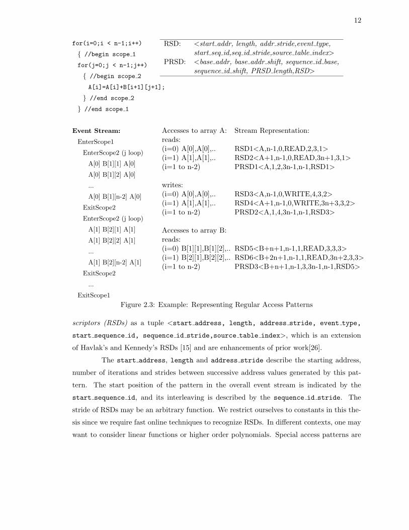
RSD: <start addr, length, addr stride,event type,start seq id,seq id stride,source table index>

PRSD: <base addr, base addr shift, sequence id base,sequence id shift, PRSD length,RSD>

Accesses to array A: Stream Representation:reads:(i=0) A[0],A[0],.. RSD1<A,n-1,0,READ,2,3,1>(i=1) A[1],A[1],.. RSD2<A+1,n-1,0,READ,3n+1,3,1>(i=1 to n-2) PRSD1<A,1,2,3n-1,n-1,RSD1>

writes:(i=0) A[0],A[0],.. RSD3<A,n-1,0,WRITE,4,3,2>(i=1) A[1],A[1],.. RSD4<A+1,n-1,0,WRITE,3n+3,3,2>(i=1 to n-2) PRSD2<A,1,4,3n-1,n-1,RSD3>

Accesses to array B:reads:(i=0) B[1][1],B[1][2],.. RSD5<B+n+1,n-1,1,READ,3,3,3>(i=1) B[2][1],B[2][2],.. RSD6<B+2n+1,n-1,1,READ,3n+2,3,3>(i=1 to n-2) PRSD3<B+n+1,n-1,3,3n-1,n-1,RSD5>

Figure 2.3: Example: Representing Regular Access Patterns

scriptors (RSDs) as a tuple <start address, length, address stride, event type,

start sequence id, sequence id stride,source table index>, which is an extension

of Havlak’s and Kennedy’s RSDs [15] and are enhancements of prior work[26].

The start address, length and address stride describe the starting address,

number of iterations and strides between successive address values generated by this pat-

tern. The start position of the pattern in the overall event stream is indicated by the

start sequence id, and its interleaving is described by the sequence id stride. The

stride of RSDs may be an arbitrary function. We restrict ourselves to constants in this the-

sis since we require fast online techniques to recognize RSDs. In different contexts, one may

want to consider linear functions or higher order polynomials. Special access patterns are

13

given by recurring references to a scalar or the same array element, which can be represented

as RSDs with a constant address stride of zero.

The event type distinguishes between reads, writes, enter scope and exit scope

events. For the scope change events, the start address field represents the scope id,

and the address stride is zero. The source table index is an index into a table of

<filename,line number> tuples. It enables the cache simulator to correlate events with

lines in the source code for user feedback.

Consider the example with a row-major layout shown in Figure 2.3. For the sake

of simplicity, we assume an offset of one per array element. The read references to array B

occur at offsets n+1, n+2, n+3 (corresponding to references B[1,1], B[1,2] and B[1,3],

respectively), for the first iteration of the outer loop and a length of n-1 accesses. The

starting sequence id for the first access of the B array is 3 (since the first three events

(seq ids start from 0) are the two enter scopes for scopes 1 and 2 as well as the read

event for A[i]). For one iteration of the outer loop, accesses to the B array occur with an

interleave distance of 3 in the overall event stream. Hence, the RSD for array B accesses for

1 iteration of the outer loop is:

RSD5 <B+n+1,n-1,1,READ,3,3,3>

Simple RSDs by themselves are not sufficiently expressive to capture the entire

stream of accesses of either array A or B. To address this limitation, we extend this de-

scription by power regular section descriptors (PRSDs), which allow the representation of

power sets of RSDs as specified in Figure 2.3. A PRSD extends the tuple of an RSD, in

that it may contain a PRSD (or RSD) itself, which represents the subset.

The recursive structure of PRSDs provides a hierarchical means to represent re-

curring patterns with different start addresses but the same strides and lengths. This is

useful for patterns that are usually encountered in nested loops.

The example in Figure 2.3 illustrates how all read accesses to array A can be

combined as follows:

PRSD1: <start base address = A,

base address shift = 1,

start base sequence id = 2,

base sequence id shift = 3n-1,

PRSD length = n-1,RSD1>

This PRSD represents a total of n-1 repetitions of RSD1 with increments of 1 in

14

addresses and interleaving distance of 3n-1 between the start of consecutive patterns in the

overall event stream.

Events that cannot be classified as a part of a pattern are represented by the

irregular access descriptor (IAD) as: <address, type, sequence id, source table index>. The

sequence id anchors the event in the overall event stream, and the source table index

gives the <filename,line number> mapping of the instruction causing this event.1 The

type indicates event type (i.e enter / exit scope or load/ store).

Once a specified number of events have been logged or a time threshold has been

reached, the instrumentation is removed, and the target is allowed to continue. The com-

pressed description of the event trace (i.e., the PRSDs & RSDs) is written to stable storage.

2.3 Online Detection of Access Patterns

This section describes our efficient online algorithm for detecting hierarchical pat-

terns in the access stream. The access stream is segregated by the unique machine code

access instruction causing the memory access. Segregation is essential since the incremental

cache simulator aggregates statistics by machine code access points as well as source code

line numbers, which are derived by mapping the machine access instruction to the source

code using the <filename,line number> tuples, as explained in the last section. Segre-

gated access streams also exhibit much better regularity, as compared to a “mixed” access

stream, since they correspond to accesses generated by the single access instruction, e.g.,

the access traces for A[i] Read, A[i] Write and B[i+1][j+1] Read in Figure 2.3 exhibit

more regularity when the array accesses are considered separately rather than as a single

composite access trace.

The compression primitives, i.e., RSDs and PRSDs, are described in the last

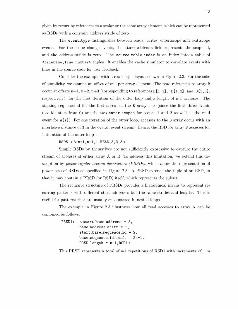
section. In our algorithm, a pattern is represented as a singly linked list. An example

pattern representation is shown in Figure 2.4, assuming each element of array A is of size

1. Each node in the linked list corresponds to a PRSD and has addr stride,seq stride,

length and height fields associated with it. The root node represents the highest level

PRSD. The Base Addr and Base Seq fields of the root node represent the starting address

and sequence number for the entire pattern. The height of a node is equal to 1 plus its

distance from the leaf node in the PRSD linked list. A node with height 0 (not shown in

1Line numbers are obtained from debugging information in the binary, as explained earlier.

15

Base_Addr = &A[0][0]Base_Seq = 0

Addr_Stride = N;

Seq_Stride = N

Length = N

Addr_Stride = 1

Seq_Stride = 1

Length = N

for(i=0;i < N;i++) for(j=0;j < N;j++) A[i][j]=0.0;

Height = 1

Height = 2

Figure 2.4: PRSD Representation

figure) is a special entity that represents a pure address element with the fields Base Addr

and Base Seq representing the address value and position in the overall stream, respectively.

For each access point, we maintain a singly linked list of levels with increasing level

number starting from 1 for the head node level. Every level can be in three possible states -

0, 1 and 2. State 0 is the default initial state for any level and represents the absence of any

element. State 1 indicates that a single PRSD is present with height=level number. State

2 indicates the presence of a meta element, i.e., a PRSD with height=level number+1.

All levels are initially in state 0. As the access stream is processed, hierarchical

PRSDs are constructed, and are propagated from lower to higher-numbered levels. Figure

2.5 shows the flowchart of processing for a single level. The instrumentation handlers

for memory accesses segregate the incoming access address by the unique machine access

instruction initiating the access. For this access point, the compression algorithm is invoked

at level 0.

Let X denote the incoming element for a level. For level 0, X represents an access

trace element with only the Base Addr and Base Seq fields valid, while for levels > 0, X is

a PRSD.

If the level is in state 0, the value of element X is stored (in Y), the level state

changes to 1, and processing ends. If the level is in state 1, the is compatible sibling

function checks whether Y (the stored element), and X (the incoming element), are compat-

ible siblings. The semantics of the is compatible sibling function are shown in Figure

2.6. If the two elements are compatible, a meta structure, i.e., a PRSD, is formed and the

level state changes to 2. The fields of this PRSD are calculated as follows:

16

Start

Element(X)IncomingRetrieve

State=0 ?Store X.

State=1.End

Form META.

State=2

State=0.

Push CurrentElement to

next level.

State=0.

All Levels

META length

Increment

OutputError

ConditionEnd

State=1 ?

State=2 ?

Yes

No

YesYes

Yes

Yes

No

No

No

is_compatible_child(X) ?

is_compatible_sibling(X) ?

>= this level

Flush

No

Figure 2.5: Flowchart: Processing at each Level

PRSD.Base Addr = X.Base Addr

PRSD.Base Seq = X.Base Seq

PRSD.Length = 2

PRSD.Addr Stride = Y.Base Addr - X.Base Addr

PRSD.Seq Stride = Y.Base Seq - X.Base Seq

PRSD.height = Y.Height + 1

If the two elements are not compatible, it indicates a change in the access pattern of the

17

access point, and we must flush any existing old patterns. So, all the resident PRSDs in the

current level and all higher-numbered levels are flushed to stable storage. Then, the current

level moves to state 0 (initial state), and we iterate again with the incoming element X.

bool is compatible sibling(sib1,sib2)

PRSD *sib1, PRSD *sib2

while(1)

/*1. check each PRSD node in linked list */

if( (sib1->length != sib2->length)

|| (sib1->addr stride != sib2->addr stride)

|| (sib1->seq stride != sib2->seq stride)

|| (sib1->height != sib2->height))

return false;

/*2. if reached end, signal success */

if( (sib1->child == NULL)

&& (sib2->child == NULL) )

return true;

/*3. height mismatch, return failure */

if( (sib1->child == NULL)

|| (sib2->child == NULL) )

return false;

/*4. now test for their children */

sib1=sib1->child;

sib2=sib2->child;

bool is compatible child(parent,child)

PRSD *parent, PRSD *child

caddr t next addr=0;

unsigned next seq=0;

int dist=0;

/*1. check height match */

if(parent->height != (child->height+1))

return false;

/*2. calculate expected address, sequence id */

dist=parent->addr stride*(parent->length);

next addr=parent->base addr+dist;

next seq=parent->base seq+dist;

/*3. check if expected match incoming */

if( (next addr != child->base addr)

|| (next seq != child->base seq))

return false;

/*4. now check lower nodes */

return is compatible sibling(parent->child,child);

Figure 2.6: Semantics of is compatible sibling & is compatible child

If the level is in state 2, it indicates that a hierarchical PRSD has been formed. The

is compatible child function checks whether the incoming element X is a valid instance

of the currently resident PRSD at this level. The semantics of the is compatible child

function are shown in Figure 2.6. If so, then the hierarchical PRSD’s length is simply

18

Intial Scenario1

Level 0. State=0

Level 1. State=0

2

3 4

Level 0. State=2

Level 0. State=1

Level 0. State=2

Level 1. State=0

Level 1. State=0

Level 1. State=0

After first access (i=0,j=0)

After second access (i=0,j=1)

Base_Seq=0

X=&A[0][0]

X=&A[0][1]Base_Addr=&A[0][0]Base_Seq=0Addr_Stride=1Seq_Stride=1Length=2Height=1

Last access on j loop,i=0 (i=0,j=N−1)

Base_Addr=&A[0][0]Base_Seq=0Addr_Stride=1Seq_Stride=1Length=NHeight=1

X=&A[0][N−1]

Height=0

Base_Addr=&A[0][0]

Figure 2.7: Illustration of the Compression Algorithm

incremented, and processing ends. If X is not a compatible child, the current resident

PRSD is pushed to the next level. Then, the current level goes to state 0, and we iterate

with the current incoming element X.

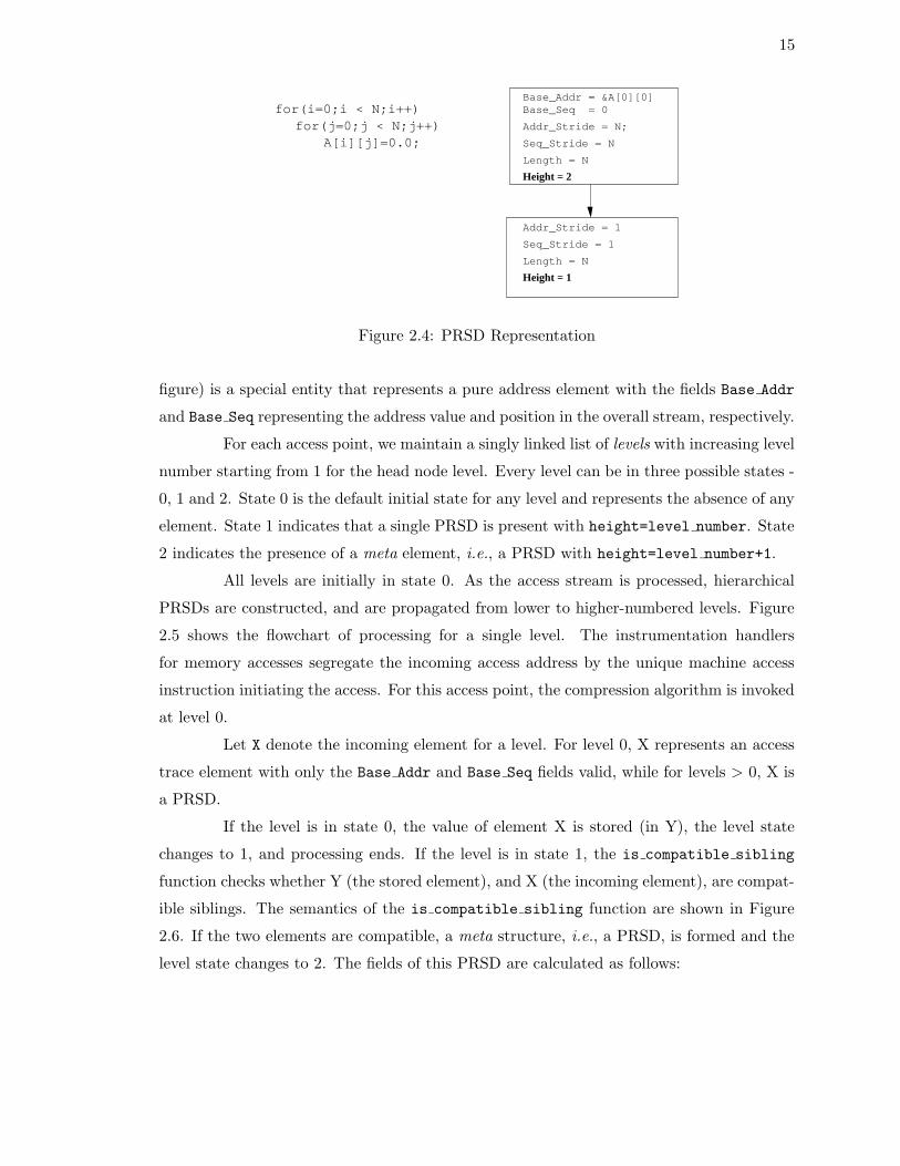
Figures 2.7 and 2.8 illustrate the compression algorithm on the C kernel shown in

19

5

Level 0. State=1

Level 1. State=1

X=&A[1][0]

6

7

Level 0. State=1 Level 0. State=2

Level 1. State=2

Level 1. State=1

Level 1. State=2

X=&A[1][N−1]Base_Addr=&A[1][0]Base_Seq=NHeight=0

After 1st access on 2nd i iteration (i=1,j=0)

Height=1Length=NSeq_Stride=1Addr_Stride=1Base_Seq=0Base_Addr=&A[0][0]

8

After last access on j loop, i=1 (i=1,j=N−1)

Level 0. State=2

Base_Addr=&A[0][0]Base_Seq=0Addr_Stride=1Seq_Stride=1Length=NHeight=1

Base_Addr=&A[1][0]Base_Seq=NAddr_Stride=1Seq_Stride=1Length=NHeight=1

After 1st access, 3rd iteration of i loop (i=2,j=0)

Base_Addr=&A[0][0]Base_Seq=0Addr_Stride=NSeq_Stride=NLength=1Height=2

Addr_Stride=1

Length=NHeight=1

Base_Seq=2NHeight=0

Base_Addr=&A[2][0]X=&A[2][0]

After last access on last iteration of i (i=N−1,j=N−1)

Base_Addr=&A[0][0]Base_Seq=0Addr_Stride=NSeq_Stride=NLength=N−2Height=2

Addr_Stride=1Seq_Stride=1Length=NHeight=1

Base_Addr=&A[N−1][0]

Addr_Stride=1Seq_Stride=1

Height=1

Base_Seq=N^2−N

Seq_Stride=1

Length=N

X=&A[N−1][N−1]

Figure 2.8: (Continued)Illustration of the Compression Algorithm

Figure 2.3, assuming each array element has size=1 and assuming row-major array layout

for simplicity.

The next sections describe the space and time complexity of the compression

algorithm.

20

2.3.1 Space Complexity

A purely random sequence without inherent patterns represents the worst case

input sequence for space complexity. It takes a linear amount of space to represent such a

sequence in our algorithm. Thus worst-case space complexity is O(M), where M is the total

number of discrete access events for the particular access point.

A regular access stream generated by a hierarchical loop nest with linear stride

functions represents the best case input sequence for space complexity. The amount of space

required to represent such a sequence is proportional to the nesting depth n of the loop nest

under discussion. As the access stream is segregated by the access point, the hierarchical

structures (PRSDs) are built separately for each point. Let the maximum number of access

points for the loop nest under consideration be p. Then, the best case space complexity is

O(n*p). Since both n and p are attributes of the code and are constant for the duration

of execution of the application, we have constant space complexity to represent nested loop

structures.

2.3.2 Time Complexity

Since we must look at all references at least once before compression, the time

complexity has a lower bound Ω(M), where M is the total number of discrete access events for

the particular access point. The following paragraphs derive the worst case time complexity

for the compression algorithm.

Consider the operation of the algorithm as shown in the flowchart in Figure 2.5.

It takes a constant number of operations for a particular level to transition from state 0 →

state 1 (operation: storing of incoming element X), and from state 1 → state 2 (operation:

formation of the meta structure). Let these constant number of operations have an upper

bound in the constant c1.

Consider the compression of accesses produced by the following abstract loop nest:

for(i1=0; i1 < len1;i1++)

for(i2=0; i2 < len2;i2++)

...................

...................

for(in=0; in < lenn;in++)

21

memory access(f(i1,i2,...,in));

Since we consider only linear strides, f(i1,i2,...,in) is assumed to be a linear

function for the analysis.

Each level li of the algorithm contains hierarchical PRSDs of height i or i+1. For

accesses generated by the above loop nest, the height of the representative PRSDs will be

bounded by the nesting depth of the loop nest, i.e., n. This is due to the nature of the

PRSD representation as each node in the PRSD linked list corresponds to a particular loop

level of the loop nest.

For a particular level li, the is compatible sibling and the is compatible child

functions must traverse all the nodes in the linked list representation of both the resident

PRSD and the incoming PRSD (X). The number of operations for this traversal is on the

order of the height of the PRSDs under consideration, i.e., O(n). Then, the exact number

of operations (ops) required to compress accesses generated by above loop nest is bounded

as:

ops ≤n

∑

i=1

(i−1∏

j=1

) ∗ (c1 + tis compatible sibling + tis compatible child ∗ (li − 2 + 1))

tis compatible sibling = # operations for is compatible sibling function. ∈ O(n)

tis compatible child = # operations for is compatible child function. ∈ O(n)

c1 = constant upper bound on # operations for transitions from state 0 → state 1 & state 1 → state

2.

(c1 + tis compatible sibling + tis compatible child*(li-2+1)) represents the number of

operations for one complete execution of the loop at depth i, Π calculates the number of

times this occurs. The summation bounds the overall number of operations for the entire

loop nest. The expression can be simplified as follows:

ops ≤n

∑

i=1

(i−1∏

j=1

lj) ∗ (c1 + tis compatible sibling + tis compatible child ∗ (li − 2 + 1)) (2.1)

≤n

∑

i=1

(i−1∏

j=1

lj) ∗ (c1 + c2 ∗ n+ c3 ∗ n ∗ li) (2.2)

≤ c1 ∗n

∑

i=1

(i−1∏

j=1

lj) + c2 ∗ n ∗n

∑

i=1

(i−1∏

j=1

lj) + c3 ∗ n ∗n

∑

i=1

(i−1∏

j=1

lj) ∗ li) (2.3)

22

Let M be the total number of accesses generated by the loop nest.

M =n

∏

k=1

lk

Using this formula to bound ops, we get:

ops ≤ c1 ∗n

∑

i=1

(i−1∏

j=1

lj) + c2 ∗ n ∗n

∑

i=1

(i−1∏

j=1

lj) + c3 ∗ n ∗n

∑

i=1

(i−1∏

j=1

lj) ∗ li) (2.4)

≤ c1 ∗

n∑

i=1

(

n∏

j=1

lj) + c2 ∗ n ∗

n∑

i=1

(

n∏

j=1

lj) + c3 ∗ n ∗

n∑

i=1

(

i∏

j=1

lj) (2.5)

≤ c1 ∗

n∑

i=1

(M) + c2 ∗ n ∗

n∑

i=1

(M) + c3 ∗ n ∗

n∑

i=1

(M) (2.6)

≤ (c1 + c2 ∗ n+ c3 ∗ n) ∗M ∗n

∑

i=1

(1) (2.7)

≤ M ∗ (c1 + c2 ∗ n+ c3 ∗ n) ∗n ∗ (n+ 1)

2(2.8)

Thus, the growth class is:

ops ∈ O(M ∗ n3)

Since n, i.e., the nesting depth, is constant and usually quite small, the algorithm

has worst case time complexity linear in the total number of references, M.

2.3.3 Comparison with Previous Work

Mueller et. al [26] introduced the PRSD, RSD and IAD compression primitives.

They also presented an online compression scheme to compress partial access traces. We

compare and contrast our algorithm with this compression scheme in Figure 2.9.

2.4 Cache Simulation and User Feedback

The compressed event trace is used for off-line incremental cache simulation. We

use a modified version of MHSim [23] as the cache simulator. MHSim was designed “to

identify source program references causing poor cache utilization, quantify cache conflicts,

temporal and spatial reuse, and correlate simulation results to references and loops in the

source code”.

23

The original MHSim package used a source-to-source Fortran translator to in-

strument data accesses with calls to the MHSim cache simulation routines. However, this

strategy has several disadvantages. Data accesses specified in the source code are simulated

in their canonical execution order, ignoring any compiler transformations that may change

the order of accesses. Additionally, the compiler may eliminate several accesses during op-

timizations (e.g., common sub-expressions). We avoid these problems by instrumenting the

application binary instead of the application source. The event trace describes the order of

accesses as they occurred during execution. The cache simulator driver uses the application

symbol table to reverse map the trace addresses to variable identifiers in the source. It relies

on the symbolic information embedded in the binary, as explained before. Every compressed

trace representation (i.e., PRSDs, RSDs and IADs) has an associated “source table index”,

which indexes into a table of <filename,line number> tuples correlating the access in-

struction in the binary to the source level access that it represents. MHSim is capable of

simulating multiple levels of memory hierarchy. However, we concentrate our analysis only

on the first level of cache (i.e., L1 cache).

For each access point, MHSim provides:

• total hits associated with the reference.

• total misses associated with the reference.

• miss ratio for the reference: basic factor in evaluating locality of reference.

• temporal reuse fraction for the reference, i.e., the number of temporal hitstotal hits

: Useful

for determining how much locality (temporal and spatial) the reference is providing.

This can be checked against the source code to see how much potential for locality

the reference actually has.

• spatial use, which is computed as used bytesblock size ∗ # evictions

, gives an indication of the

fraction of the cache block being referenced before an eviction occurs. A low spatial

use count would indicate that the machine is wasting cycles and/or space bringing in

data that is never referenced.

• evictor references: the identities of the competing references which evicted this

reference from the cache, and their relative counts. These are useful for determining

24

which data objects conflict with each other. The conflict can be resolved by program

transformations or by data reorganization (e.g., array padding).

25

Our Algorithm Previous Algorithm

Description Description• Access traces segregated by accesspoint.

• Every access point is associated withnumbered levels; a level li can con-tain a PRSD of height i or i+1.

• PRSDs are propagated from lowerto higher-numbered levels wherethey combine to form higher orderPRSDs.

• Maintain pool table, a block of ad-dresses to be compressed.

• A difference table calculates dif-ferences between pool elements;RSDs are located by finding se-quence of pool elements with iden-tical difference values.

Ordering of Accesses Ordering of AccessesGlobally unique sequence ids are associ-ated with each PRSD, ensuring global or-dering and interleaving among all pat-terns.

Two streams are ordered relative to eachother, using the interleave vector(IV). Thetwo streams, plus the IV, forms the datastream(DS), which can be further orderedrelative to others data streams using IVs.

Time Complexity: O(M x n3) Time Complexity: O(M x w2)M = total # accesses M = total # accesses

n = nesting depth of loop nest w = width of pool table

(Time complexity only for RSD detection)

Space Complexity: Space Complexity:O(M), Ω(n*p) O(M), Ω(n)

M = total # accesses M = total # accesses

n = nesting depth, p = # access pts. n = nesting depth

Pros Pros

• Since n is a small constant, worstcase time complexity linear in the to-tal number of references.

• Provides access point segregated ac-cess traces; essential for correlatingmemory statistics to source code.

• Trade-off possible between compres-sion overhead and level of compres-sion, by varying the pool width w.

• Since access streams are not segre-gated, can exploit pattern regularityacross access points, resulting in po-tentially improved compression.

Cons Cons• Potential compression using patternregularity across access points islost, due to stream segregation

• Current algorithm considers accesswith only linear strides.

• Cannot be used for METRIC, sinceaccesses from different access pointsare not distinguished.

• Potentially slower, since the com-posite access stream rather than theaccess-point-segregated stream mustbe scanned for patterns

Figure 2.9: A Comparison of Our Algorithm with Previous Work

26

Chapter 3

Case Studies

In this chapter, we illustrate the use of our framework to analyze the locality

behavior of several test kernels. We show how the cache simulation results can be used to

detect and isolate bottlenecks and to derive appropriate program transformations.

The cache configuration had the following parameters: cache size of 32 KB, 32-

byte line size, 2-way associativity, LRU cache replacement policy. A partial data trace was

obtained for each kernel. The compressed trace was run through the cache simulator to

produce memory hierarchy statistics.

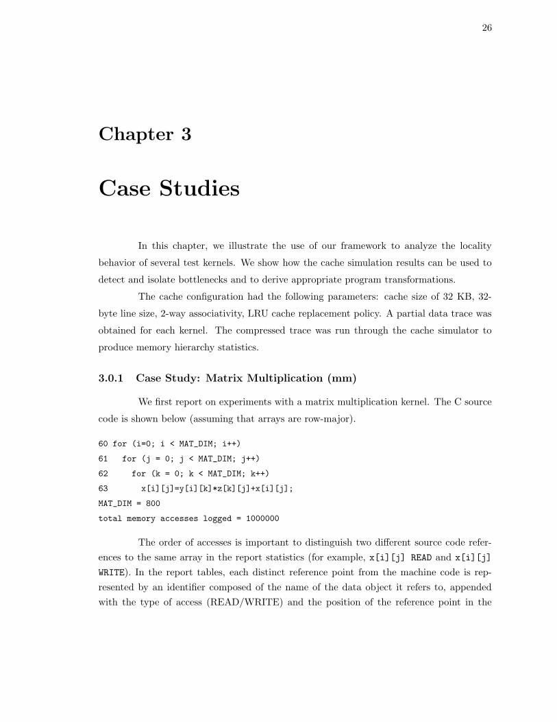
3.0.1 Case Study: Matrix Multiplication (mm)

We first report on experiments with a matrix multiplication kernel. The C source

code is shown below (assuming that arrays are row-major).

60 for (i=0; i < MAT_DIM; i++)

61 for (j = 0; j < MAT_DIM; j++)

62 for (k = 0; k < MAT_DIM; k++)

63 x[i][j]=y[i][k]*z[k][j]+x[i][j];

MAT_DIM = 800

total memory accesses logged = 1000000

The order of accesses is important to distinguish two different source code refer-

ences to the same array in the report statistics (for example, x[i][j] READ and x[i][j]

WRITE). In the report tables, each distinct reference point from the machine code is rep-

resented by an identifier composed of the name of the data object it refers to, appended

with the type of access (READ/WRITE) and the position of the reference point in the

27

Miss Temporal SpatialFile Line Reference Source Ref Hits Misses Ratio Ratio Use

mm.c 63 z Read 1 z[k][j] 0 2.50e+05 1.00 no hits 0.171mm.c 63 y Read 0 y[i][k] 2.39e+05 1.10e+04 0.0441 0.854 0.129mm.c 63 x Read 2 x[i][j] 2.50e+05 1.57e+02 0.0006 1.00 0.5mm.c 63 x Write 3 x[i][j] 2.50e+05 0.0 0.0 1.00 no evicts

Figure 3.1: Per-Reference Cache Statistics for Unoptimized Matrix Multiply

Reference EvictorsFile Line Name Source Ref File Line Name Source Ref Count Percent

mm.c 63 y Read 0 y[i][k] mm.c 63 z Read 1 z[k][j] 10863 100.00

mm.c 63 z Read 1 z[k][j] mm.c 63 z Read 1 z[k][j] 238150 95.58mm.c 63 y Read 0 y[i][k] 10854 4.36mm.c 63 x Read 2 x[i][j] 149 0.06

mm.c 63 x Read 2 x[i][j] mm.c 63 z Read 1 z[k][j] 149 100.00

mm.c 63 x Write 3 x[i][j] mm.c 63 z Read 1 z[k][j] 149 100.00

Figure 3.2: Evictor Information for Unoptimized Matrix Multiply

overall order of accesses in the binary. (For example, in the untiled matrix multiply ker-

nel’s machine code, the order of accesses is y(read), z(read), x(read), x(write) indicated

as y Read 0, z Read 1, x Read 2 and x Write 3, respectively.) We observe the following

overall performance:

reads = 750000 temporal hits = 703930writes = 250000 spatial hits = 34881hits = 738811 temporal ratio = 0.95279misses = 261189 spatial ratio = 0.04721miss ratio = 0.26119 spatial use = 0.16980

The high miss rate (26%) should be the first indication of concern for the analyst.

Interestingly, the spatial use value is quite low (0.16980). This indicates that the current

program referencing order is inefficient in the sense that most cache blocks are being evicted

before the entire data in the block is referenced at least once.

Let us explore the cache statistics at a higher level of detail. Refer to Figure 3.1

28

Miss Temporal SpatialFile Line Reference Source Ref Hits Misses Ratio Ratio Use

mm.c 86 x Read 2 x[i][j] 2.41e+05 8.79e+03 0.0352 0.972 0.673mm.c 86 y Read 0 y[i][k] 2.41e+05 8.79e+03 0.0352 0.896 0.732mm.c 86 z Read 1 z[k][j] 2.50e+05 2.88e+02 0.0011 0.999 0.861mm.c 86 x Write 3 x[i][j] 2.50e+05 0.00e+00 0.0 0.989 no evicts

Figure 3.3: Per-Reference Cache Statistics for Optimized Matrix Multiply

for the per-reference cache statistics. The z Read 1 performance is immediately striking.

All accesses to the z array were misses. A look at the source indicates the cause: The k

loop runs over the rows of z. By the time reuse of z data occurs (on next iteration of the i

loop), the data has been flushed from the cache. With only a single element of the cache

line containing z being referenced for each iteration of k, the spatial use value is also low

(0.171).

With the x Read 2 reference, the number of hits is large, as expected, since the

x[i][j] read is invariant for the k loop. Even here, however, the spatial use is low (0.5)

indicating premature eviction before all data in the block was referenced. The x Write 3

writes to data locations already brought into cache by the x Read 2 reference, explaining a

miss rate of 0.

For the y Read 0 reference, the number of hits is quite large, comparable in mag-

nitude to the hits for the x Read 2 reference. A surprising feature is the relatively high

temporal ratio (0.854). With the k loop running over the column dimension of y and

temporal reuse not occurring till next iteration of j, we would rather expect the temporal

fraction of hits to be low. This means that the y Read 0 reference does not experience

too much interference from other references over long stretches of accesses (more than the

length of the k loop).

The evictor table for mm is shown in Figure 3.2. Again, the z Read 1 reference

performance is unusual. Over 95% of the time, z Read 1 interfered with itself, indicating a

capacity problem. Additionally, z Read 1 was the evictor for all the other references (100%

of the time). These evictions by z cause premature invalidation of block data belonging to

evicted references, leading to low spatial use (and, thus, low overall cache usage efficiency)

for these references.

Improving data locality: We have pinpointed the z array references as having

29

Reference EvictorsFile Line Name Source Ref File Line Name Source Ref Count Percent

mm.c 86 z Read 1 z[k][j] mm.c 86 y Read 0 y[i][k] 100 69.44mm.c 86 x Read 2 x[i][j] 42 29.17mm.c 86 z Read 1 z[k][j] 2 1.39

mm.c 86 x Read 2 x[i][j] mm.c 86 x Read 2 x[i][j] 4976 60.05mm.c 86 y Read 0 y[i][k] 3297 39.79mm.c 86 z Read 1 z[k][j] 14 0.17

mm.c 86 x Write 3 x[i][j] mm.c 86 x Read 2 x[i][j] 4976 60.05mm.c 86 y Read 0 y[i][k] 3297 39.79mm.c 86 z Read 1 z[k][j] 14 0.17

mm.c 86 y Read 0 y[i][k] mm.c 86 y Read 0 y[i][k] 5010 59.52mm.c 86 x Read 2 x[i][j] 3279 38.96mm.c 86 z Read 1 z[k][j] 128 1.52

Figure 3.4: Evictor Information for Optimized Matrix Multiply

the maximum effect on cache performance. We need to change the program structure to

reduce the access footprint for z. By interchanging the j and k loops, we can increase

locality for z (since now the inner loop runs over the columns of z), which has the highest

number of misses. By strip mining the j and k loops, we can force the temporal reuse to

occur at shorter intervals in the overall event stream, especially for arrays y and x. This

will reduce the chance of these references having blocks flushed from the cache before the

entire block data is utilized. The new transformed code with these improvements is shown

below.

81 for (jj=0; jj<MAT_DIM; jj += ts)

82 for (kk=0; kk<MAT_DIM; kk += ts)

83 for (i=0; i<MAT_DIM; i++)

84 for (k=kk; k<min(kk+ts,MAT_DIM); k++)

85 for (j=jj; j<min(jj+ts,MAT_DIM); j++)

86 x[i][j]=y[i][k]*z[k][j]+x[i][j];

tile size ts = 16;

We observe the following overall performance:

30

reads = 750000 temporal hits = 947173writes = 250000 spatial hits = 34955hits = 982128 temporal ratio = 0.96441misses = 17872 spatial ratio = 0.03559miss ratio = 0.01787 spatial use = 0.70394

Figures 3.3 and 3.4 show the per-reference cache statistics and the evictor table

for the transformed matrix multiply code. Figures 3.5(a-c) contrast the results before and

after optimization for misses, use and evictor information for the critical reference z Read 1,

respectively.

The overall miss ratio has decreased two orders of magnitude from 0.26 to 0.017.

The overall spatial use has also improved greatly from 0.16980 to 0.70394. The greatest

improvement has occurred for the z Read 1 reference; the number of hits has gone down

from 0 to 2.5e+05, with 99.9% of these being temporal hits.

Also, for all references, the spatial use values have gone up, increasing the efficiency

of cache usage. The eviction table in Figure 3.4 why this happened. The number of evictions

for most references has gone down significantly, especially for the z reference from almost

240,000 to less than 200. Evictors for this reference are also depicted in Figure 3.5(c).

For other references, the evictors are mostly references to the same array. Overall, the

interference between the z reference and other references has been significantly reduced with

a slight overall increase in interference between other references (e.g., between y Read 0 and

x Read 2).

Consider the pseudo-code for the unoptimized matrix multiply again. Two ref-

erences to x, a read and a write, are inflicted on one array element. We performed our

experiments by compiling without allocating x[i][j] to a register in the inner loop. While

register allocation would have affected the total number of references for x, it has a neg-

ligible impact on eviction and miss ratios, as verified by the low eviction count of 149 in

Figure 3.2. Only one out of 800 array references would have been affected in arrays y and

z. In the optimized case, allocating y to a register would have had a similar affect since the

cache associativity was two and both tiled blocks of x and y could co-exist in cache.

31

(a) Total Number of Misses

(b) Spatial User per Reference

(c) Evictors for z Read 1 (log scale)

Figure 3.5: Contrasted Metrics for Matrix Multiply before and after Optimizations

32

3.0.2 Case Study: Erlebacher ADI Integration

The C kernel for the Erlebacher ADI Integration is shown below. For this kernel,

the possible optimizations (loop interchange and fusion) are visually apparent. However,

we illustrate how the cache results can be used to divine the need for these optimizations.

The result analysis would be similar in the case of more non-obvious codes benefiting from

the same loop optimizations.

16 for (k = 1; k < N; k++)

17 for (i = 2; i < N; i++)

18 x[i][k] = x[i][k] - x[i-1][k]*a[i][k] /b[i-1][k];

19 for (i = 2; i < N; i++)

20 b[i][k] = b[i][k] - a[i][k] * a[i][k] /b[i-1][k];

21

N = 800

total memory accesses logged = 1000000

We observe the following overall performance:

reads = 800000 temporal hits = 351731writes = 200000 spatial hits = 147768hits = 499499 temporal ratio = 0.70417misses = 500501 spatial ratio = 0.29583miss ratio = 0.50050 spatial use = 0.20181

As in mm, the primary indicator of concern is the miss ratio — over 50% of the total accesses

are misses. Spatial hits constitute just a third of the overall hits. The low spatial use value

(0.20) indicates the poor efficiency of the current program order of memory accesses.

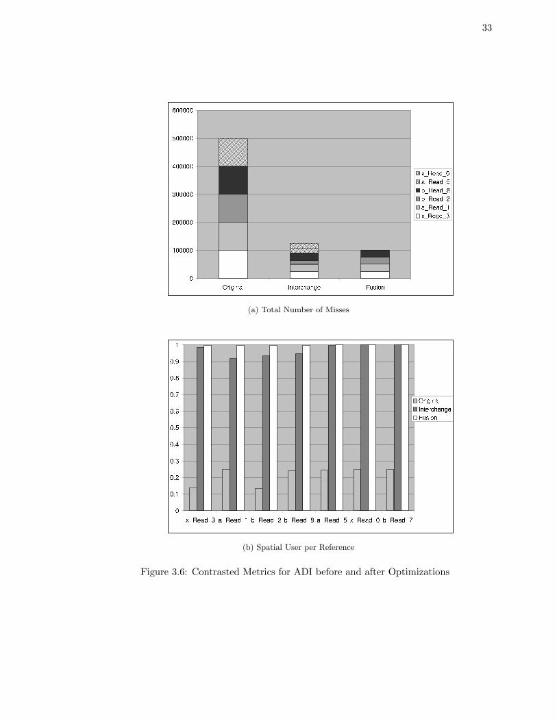
The reference-specific statistics are summarized in the first bar of Figure 3.6(a).

In addition, Figure 3.6(b) indicates low spatial use for read references in the original code.

The first five references x[i][k], a[i][k], b[i-1][k],b[i][k] and a[i][k] do not have

a single hit in the cache. Looking at the source code, a common pattern is evident among

all these reference: the inner loop (i loop) runs over the rows of these references. Spatially

adjacent elements from these arrays, in the same cache block as these references, are accessed

only on the next iteration of the k loop, by which time they have been flushed from the

cache. Hence, spatial use value is low, and spatial hits are negligible.

The evictor information (not shown due to its size) actually indicates this problem

independent of source code knowledge. A circular dependency exists for the references and

33

(a) Total Number of Misses

(b) Spatial User per Reference

Figure 3.6: Contrasted Metrics for ADI before and after Optimizations

34

their evictors within both inner loops. We need to reorder the accesses so that we can take

advantage of spatial reuse by running the inner loop over the columns (rather than rows)

of these references. The source code indicates that this is possible without violating data

dependencies.

Improving Locality: The loop-interchanged kernel is shown below.

16 for (i = 2; i < N; i++)

17 for (k = 1; k < N; k++)

18 x[i][k] = x[i][k] - x[i-1][k] * a[i][k] /b[i-1][k];

19 for (k = 1; k < N; k++)

20 b[i][k] = b[i][k] - a[i][k] * a[i][k] /b[i-1][k];

21

We observe the following overall performance:

reads = 800000 temporal hits = 454867writes = 200000 spatial hits = 419733hits = 874600 temporal ratio = 0.52009misses = 125400 spatial ratio = 0.47991miss ratio = 0.12540 spatial use = 0.96281

There is significant improvement in the miss ratio: it has fallen from 50% to less than 13%

in the optimized code. The access efficiency, indicated by the spatial use, has increased

drastically from 0.20 to 0.96.

Can we optimize the locality further? To determine this, we need to look at the

reference-specific statistics, summarized for selected references in the second bar of Figure

3.6(a). The miss ratio has decreased substantially, especially for the five references we

focused on ( x Read 3, a Read 1, b Read 2, b Read 8, a Read 5) in the analysis of the

unoptimized kernel. However, there still remain a non-negligible number of misses. If we

look at the source names for the references, we see that there are a lot of common expressions

(especially a[i][k] and b[i][k]). Grouping these accesses together would further increase

locality for the secondary accesses to the same array (e.g., grouping a Read 1 and a Read 5

would eliminate misses for a Read 5). Of course, this transformation would be possible only

if no data dependencies are violated. The new kernel is shown below.

14 for (i = 2; i < N; i++)

15 for (k = 1; k < N; k++)

16 x[i][k] = x[i][k] - x[i-1][k] * a[i][k] / b[i-1][k];

35

17 b[i][k] = b[i][k] - a[i][k] * a[i][k] / b[i-1][k];

18

We observe the following overall performance:

reads = 800000 temporal hits = 549822writes = 200000 spatial hits = 349849hits = 899671 temporal ratio = 0.61114misses = 100329 spatial ratio = 0.38886miss ratio = 0.10033 spatial use = 0.99798

The miss ratio has decreased from 12.5% to 10%. The temporal use increased due to

grouping of accesses, leading to approximately 5% increase in temporal hits. As a side-

effect of the reduced number of evictions (directly correlated to reduction in total misses),

the spatial use has increased to 0.997, indicating excellent access efficiency.

The last bar in Figure 3.6(a) shows the per-reference statistics for the loop-fused

case. The table indicates that the chief improvement has been in the a Read 5 and x Read 0

references. Grouping the a[i][k] access for a Read 5 and a Read 1 caused the misses for

a Read 5 to go down to zero. The x Read 0 reference also decreased its number of misses

by over two orders of magnitude, leading to a miss ratio of almost 0. This is surprising since

the reuse for the x[i-1][k] element (due to the x[i][k] read reference) occurs only on the

next iteration of the i loop. The reduction in the overall misses (and, thus, the evictions)

due to grouping seems to have reduced the cross-interference for the x[i-1][k] reference

as a side effect.

Careful analysis of the statistics reveals there is still potential for improvement.

The x Read 3 (x[i][k]) and x Read 0 (x[i-1][k]) as well as b Read 2 (b[i-1][k]) and

b Read 8 (b[i][k]) share temporal reuse potential on adjacent iterations of the i loop. The

misses for x Read 0 and b Read 8 can be reduced by tiling (blocking) for the i and k loops.

However, we will not discuss these modifications here.

36

Chapter 4

Validation Experiments

This chapter describes our experiments to characterize performance aspects of the

METRIC framework. The test suite consists of 4 benchmarks- SPEC-swim, adi, matrix

multiply and tiled matrix multiply. The experiments were carried out on an IBM SP

system with four Power3-II processors.

4.1 Experiment 1. Accuracy of Simulation

This experiment measures the accuracy of the incremental cache simulator, com-

pared to hardware performance counters. For each test application, a partial access trace

of 1 Million accesses was collected using the METRIC framework’s facility for collecting

partial access traces. This trace was used to generate results from the incremental cache

simulator. The results were compared against performance counter values obtained using

the libhpm API, a part of the IBM Hardware Performance Monitor Toolkit (HPM). The

hardware counts were collected using the batch mode of execution, rather than on interac-

tive nodes of the IBM SP system, to minimize the effects of extraneous processes on the

processor’s cache. We only investigated metrics related to the L1 data cache loads.

Figure 4.1 compares the load misses reported by HPM to the load misses reported

by the cache simulator. We observe that there is a difference between the numbers reported

by the two approaches. There could be several causes for this. Figure 4.2(a) shows the num-

ber of context switches that occured during monitoring, as reported by HPM. Performance

counter values are saved by the kernel whenever the process being monitored undergoes a

context switch. However, the execution of the other processes still impacts the processor

37

Figure 4.1: Comparison of load misses reported by HPM and Cache Simulator

cache, leading to higher number of misses being reported by HPM. Figure 4.2(b) shows the

number of page faults that occured during monitoring, as reported by HPM. Page faults

do not cause context switches, however they cause the page fault handler to execute, which

can also impact the processor cache.

The METRIC framework aggregates results at various levels of detail, such as

functions, loops, line numbers and data structures. However, hardware performance coun-

ters cannot provide this level of detail. Thus, METRIC makes available highly detailed

performance statistics, with acceptable accuracy for the tested benchmarks.

4.2 Experiment 2. Compression Rate

This experiment measures the effectiveness of the online trace compression algo-

rithm. Effective compression is critical since writing excessive amounts of data to stable

storage will slow down the target application and require large amounts of stable storage

space.

38

(a) # context switches (b) # page faults

Figure 4.2: Potential Causes of Cache Interference

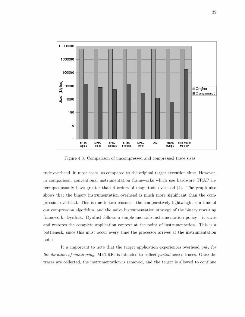
For each test application, a partial access trace of 1 Million accesses was collected.

For the uncompressed trace, the trace size was calculated as 1 Million * (size of 1 trace

element). Each trace element has two components - the 32-bit address and the 16-bit

source table index, which maps the access to the unique machine access instruction that

generated it. Thus, for all benchmarks, the size of the uncompressed trace = 1 Million * 6

= 6 Million bytes.

Figure 4.3 compares the relative sizes of the uncompressed and compressed trace.

The y-axis is in logarithmic scale. In most cases, the access trace is compressed by greater

than 2 orders of magnitude indicating a significant decrease in the amount of trace data

required to be written to stable storage.

4.3 Experiment 3. Execution Overhead

This experiment measures the execution overhead induced by the trace collection

framework for the target application. This overhead has two components - the overhead of

the binary instrumentation framework and the overhead of the compression algorithm. The

instrumentation overhead consists of the instructions needed to save and restore machine

context at the point of instrumentation.

Figure 4.4 plots the execution overhead for the framework. NULL Instrumentation

and Instrumentation+Compression depict the overheads for the binary instrumentation

without and with trace compression, respectively. There is two to three orders of magni-

39

Figure 4.3: Comparison of uncompressed and compressed trace sizes

tude overhead, in most cases, as compared to the original target execution time. However,

in comparison, conventional instrumentation frameworks which use hardware TRAP in-

terrupts usually have greater than 4 orders of magnitude overhead [4]. The graph also

shows that the binary instrumentation overhead is much more significant than the com-

pression overhead. This is due to two reasons - the comparatively lightweight run time of

our compression algorithm, and the naive instrumentation strategy of the binary rewriting

framework, DynInst. DynInst follows a simple and safe instrumentation policy - it saves

and restores the complete application context at the point of instrumentation. This is a

bottleneck, since this must occur every time the processor arrives at the instrumentation

point.

It is important to note that the target application experiences overhead only for

the duration of monitoring. METRIC is intended to collect partial access traces. Once the

traces are collected, the instrumentation is removed, and the target is allowed to continue

40

Figure 4.4: Execution Overhead in Target Execution

unaffected, while cache simulation takes place in a separate process or even on a separate

machine.

41

Chapter 5

Related Work

Regular Section Descriptors represent a particular instance of a common concept in

memory optimizations, either in software or hardware. For instance, Havlak and Kennedy’s

RSDs [15] are virtually identical to the stream descriptors in use at about the same time in

the compiler and memory systems work inspired by the WM architecture [34].

ATOM has been widely used as a binary rewriting tool to statically insert in-

strumentation code into application binaries [28]. Dynamic binary rewriting enhances this

approach by its ability to dynamically select place and time for instrumentations. This

allows the generation of partial address traces, for example, for frequently executed regions

of code and a limited number of iterations with a code section. In addition, DynInst makes

dynamic binary rewriting a portable approach.

Weikle et al. [31] describe an analytic framework for the evaluation of caching

systems. Their approach views caches as filters, and one component of the framework is

a trace-specification notation called TSpec. TSpec is similar to the RSDs described here

in that it provides a more formal mechanism by which researchers may communicate with

clarity about the memory references generated by a processor. The TSpec notation is more

complex than RSDs, since it is also the object on which the cache filter operates and is used

to describe the state of a caching system. All such notations support the creation of tools

for automatic trace expansion or synthetic trace generation, and can be used to represent

different levels of abstraction in benchmark analysis.

Buck and Hollingsworth performed a simulation study to pinpoint the hot spots

of cache misses based on hardware support for data trace generation [5]. Hardware counter

support in conjunction with interrupt support on overflow for a cache miss counter was

42

compared to miss counting in selected memory regions. The former approach is based on

probing to capture data misses at a certain frequency (e.g., one out of 50,000 misses). The

latter approach performs a binary search (or n-way search) over the data space to identify

the location of the most frequently occurring misses. Sampling was reported to yield less

accurate results than searching. The approach based on searching provided accurate results

(mostly less than 2% error) for these simulations. Unfortunately, hardware support for

either of these two approaches is not yet readily available (with the exception of the IA-64).

In addition, interrupts on overflow are imprecise due to instruction-level parallelism. The

data reference causing an interrupt is only known to be located in “close vicinity” to the

interrupted instruction, which complicates the analysis. Finally, this described hardware

support is not portable. In contrast, our approach to generating traces is applicable to

today’s architectures, is portable and precise in locating data references, and does not

require the overhead of interrupt handling. Other approaches to determining the causes of

cache misses, such as informing memory operations, are also based on hardware support

and are presently not supported in contemporary architectures [17, 25].

Recent work by Mellor-Crummey et al. uses source-to-source translation on HPF

to insert instrumentation code that extracts a data trace of array references. The trace

is later exposed to a cache simulator before miss correlations are reported [23]. CProf

[20] and MemSpy[22] are similar tools that rely on post link-time binary editing through

EEL[18, 19] and Tango[11] respectively, but cannot handle shared library instrumentation

or partial traces. Lebeck and Wood also applied binary editing to substitute instructions

that reference data in memory with function calls to simulate caches on-the-fly [21]. Our

work differs in the fundamental approach of rewriting binaries, which is neither restricted

to a special compiler or programming language, nor does it preclude the analysis of library

routines. Another major difference addresses the overhead of large data traces inherent to

all these approaches. We restrict ourselves to partial traces and employ trace compression

to provide compact representations.

Recent work by Chilimbi et al. concentrates on language support and data layout

to better exploit caches [9, 8] as well as quantitative metrics to assess memory bottlenecks

within the data reference stream [7]. This work introduces the term whole program stream

(WPS) to refer to the data reference stream, and presents methods to compactly represent

the WPS in a grammatical form. Other efforts concentrate on access modeling based on

whole program traces [4, 12] using cache miss equations [13] or symbolic reference analysis

43

at the source level based on Presburger formulas [6]. These approaches involve linear solvers

with response times on the order of several minutes up to over an hour. We concentrate

our efforts on providing feedback to a programmer quickly.

SIGMA is a tool using binary rewriting through Augment6k to analyze memory

effects [12]. This is the closest related work. SIGMA captures full address traces through

binary rewriting. Experimental results show a good correlation to hardware counters for

cache metric of entire program executions. Performance prediction and tuning results are

also reported, which are subject to manual padding of data structures in a second compila-

tion pass in response to cache analysis. Their approach differs in that they neither capture

partial access traces nor present a concept for such an approach. Their trace compression

algorithm is inferior, in the sense that it cannot efficiently compress access streams where

regular data accesses are interleaved with non-regular accesses (e.g., accesses to A[i] and

B[C[i]] alternating in a loop). By segregating the access stream by the point of access,

and associating ordering information (sequence ids) with each trace pattern separately,

we can compress such access patterns much better. Our cache analysis is more powerful.

It reports not only per-reference metrics but also per-reference evictor information, which

is imperative to infer the potential for optimizations. Subsequently, we are able to apply

more sophisticated optimizations, such as tiling and loop transformations.

44

Chapter 6

Conclusions and Future Work

This thesis describes a novel application of dynamic binary rewriting for detecting

inefficiencies in memory reference patterns. Our contributions are a portable framework

(METRIC) for selective instrumentation of load and store instructions on-the-fly, the

generation and compression of partial access traces as well as the simulation of reference

behavior in terms of caching. We present an efficient online compression algorithm and

derive the worst case time and space complexity for it. Our enhanced memory hierarchy

simulator allows correlation of detailed cache metrics and evictor information to source code

and data structures, allowing sources of memory access inefficiencies to be localized. The

case studies presented illustrate how the detailed information made available by the frame-

work allows us to infer the potential for program transformations. These transformations

result in an absolute miss reduction of up to 40% for the case studies discussed. We also

validated the simulator accuracy against hardware performance counters, demonstrated the

efficiency of the compression algorithm and analyzed trace collection overheads for a range

of benchmarks.

METRIC represents the first step toward a tool that alters long-running programs

on-the-fly so that their speed increases over their execution lifetime - without any recompi-

lation or user interaction. Initially, we plan to benchmark METRIC with additional SPEC

benchmarks from the SPEC2000 benchmark suite. Next, we shall investigate the the ap-

plication of program analysis and subsequently, dynamic optimization on the binary. This

requires not only the reconstruction of the control-flow graph, which is available at the bi-

nary level, but also the calculation of data-flow information and the detection of induction

variables in order to infer data dependencies and dependence distance vectors[32, 33], a pre-

45

requisite to determine if certain program transformations preserve the program semantics.

46

Bibliography

[1] V. Bala, E. Duesterwald, and S. Banerjia. Dynamo: A transparent dynamic optimiza-

tion system. In ACM SIGPLAN Conference on Programming Language Design and

Implementation, pages 1–12, June 2000.

[2] Rudolph Berrendorf and Heinz Ziegler. Pcl - the performance counter library:

A common interface to access hardware performance counters on microprocessors.

http://www.fz-juelich.de/zam/PCL/.

[3] S. Browne, J. Dongarra, N. Garner, K. London, and P. Mucci. A scalable cross-platform

infrastructure for application performance tuning using hardware counters. In SC’2000,

November 2000.

[4] Bryan Buck and Jeffrey K. Hollingsworth. An API for runtime code patching. The

International Journal of High Performance Computing Applications, 14(4):317–329,

Winter 2000.

[5] Bryan R. Buck and Jeffrey K. Hollingsworth. Using hardware performance monitors

to isolate memory bottlenecks. In Supercomputing, pages 64–65, November 2000.

[6] S. Chatterjee, E. Parker, P. Hanlon, and A. Lebeck. Exact analysis of the cache

behavior of nested loops. In ACM SIGPLAN Conference on Programming Language

Design and Implementation, pages 286–297, June 2001.

[7] Trishul Chilimbi. Efficient representations and abstractions for quantifying and exploit-

ing data reference locality. In ACM SIGPLAN Conference on Programming Language

Design and Implementation, pages 191–202, June 2001.

[8] Trishul M. Chilimbi, Bob Davidson, and James R. Larus. Cache-conscious structure

47

definition. In ACM SIGPLAN Conference on Programming Language Design and Im-

plementation, pages 13–24, May 1999.

[9] Trishul M. Chilimbi, Mark D. Hill, and James R. Larus. Cache-conscious structure

layout. In ACM SIGPLAN Conference on Programming Language Design and Imple-

mentation, pages 1–12, May 1999.

[10] Intel Corp. Intel IA-64 Architecture Software Developer’s Manual, volume 4. 2000.

[11] H. Davis, S. Goldschmidt, and J. Hennessy. Tango: A multiprocessor simulation and

tracing system. In Proceedings of the International Conference on Parallel Processing,

pages 99–107, August 1991.

[12] L. DeRose, K. Ekanadham, J K. Hollingsworth, and S. Sbaraglia. SIGMA: A simulator

infrastructure to guide memory analysis. In Supercomputing, November 2002.

[13] Somnath Ghosh, Margaret Martonosi, and Sharad Malik. Cache miss equations: a

compiler framework for analyzing and tuning memory behavior. ACM Transactions

on Programming Languages and Systems, 21(4):703–746, 1999.

[14] S. L. Graham, P. B. Kessler, and M. K. McKusick. gprof: A call graph execution

profiler. In Symposium on Compiler Construction, pages 276–283, June 1982.

[15] Paul Havlak and Ken Kennedy. An implementation of interprocedural bounded regular

section analysis. IEEE Transactions on Parallel and Distributed Systems, 2(3):350–360,

July 1991.

[16] J.L. Hennessy and D.A. Patterson. Computer Organization and Design. Morgan Kauf-

mann, 2nd edition, 1997.

[17] Mark Horowitz, Margaret Martonosi, Todd C. Mowry, and Michael D. Smith. In-

forming memory operations: Providing memory performance feedback in modern pro-

cessors. In International Symposium on Computer Architecture, pages 260–270, May

1996.

[18] James R. Larus and Thomas Ball. Rewriting executable files to measure program

behavior. Software Practice & Experience, 24(2):197–218, February 1994.

48

[19] James R. Larus and Eric Schnarr. EEL: Machine-independent executable editing. In

ACM SIGPLAN Conference on Programming Language Design and Implementation,

pages 291–300, June 1995.

[20] Alvin R. Lebeck and David A. Wood. Cache profiling and the SPEC benchmarks: A

case study. Computer, 27(10):15–26, October 1994.

[21] Alvin R. Lebeck and David A. Wood. Active memory: A new abstraction for memory

system simulation. ACM Transactions on Modeling and Computer Simulation, 7(1):42–

77, January 1997.

[22] Margaret Martonosi, Anoop Gupta, and Thomas E. Anderson. Memspy: Analyzing

memory system bottlenecks in programs. In Measurement and Modeling of Computer

Systems, pages 1–12, 1992.

[23] J. Mellor-Crummey, R. Fowler, and D. Whalley. Tools for application-oriented perfor-

mance tuning. In International Conference on Supercomputing, pages 154–165, June

2001.

[24] Shirley V. Moore. A comparison of counting and sampling modes of using performance

monitoring hardware. In Proceedings of the International Conference on Computional

Science, 2002.

[25] T. C. Mowry and C.-K. Luk. Predicting data cache misses in non-numeric applications

through correlation profiling. In MICRO-30, pages 314–320, December 1997.

[26] F. Mueller, T. Mohan, B. R. de Supinski, S. A. McKee, and A. Yoo. Partial data

traces: Efficient generation and representation. In Workshop on Binary Translation,

IEEE Technical Committee on Computer Architecture Newsletter, October 2001.

[27] David Patterson, Thomas Anderson, Neal Cardwell, Richard Fromm, Kimberly Keeton,

Christoforos Kozyrakis, Randi Thomas, and Katherine Yelick. A case for intelligent

RAM. IEEE Micro, 17(2):34–44, 1997.

[28] Amitabh Srivastava and Alan Eustace. ATOM: A system for building customized

program analysis tools. In ACM SIGPLAN Conference on Programming Language

Design and Implementation, pages 196–205, June 1994.

49

[29] R. Uhlig and T. Mudge. Trace-driven memory simulation: A survey. ACM Trans.

Computing Surveys, 29(2):128–170, June 1997.

[30] J. Vetter and F. Mueller. Communication characteristics of large-scale scientific ap-

plications for contemporary cluster architectures. In International Parallel and Dis-

tributed Processing Symposium, April 2002.

[31] D.A.B. Weikle, S.A. McKee, Kevin Skadron, and Wm.A. Wulf. Caches as filters: A

framework for the analysis of caching systems. In Grace Murray Hopper Conference,

September 2000.

[32] M. E. Wolf and M. S. Lam. A data locality optimizing algorithm. In ACM SIGPLAN

Conference on Programming Language Design and Implementation, pages 30–44, June

1991.

[33] M. Wolfe. High Performance Compilers for Parallel Computing. Addison-Wesley, 1996.

[34] W.Wulf. Evaluation of the WM architecture. In International Symposium on Computer

Architecture, pages 382–390, May 1992.