Embed Size (px)
Citation preview

Abstract
The thesis addresses the problem of space-time codebook design for communication
in multiple-input multiple-output (MIMO) wireless systems. The realistic and challeng-
ing non-coherent setup (channel state information is absent at the receiver) is considered.
A generalized likelihood ratio test (GLRT)-like detector is assumed at the receiver and
contrary to most existing approaches, an arbitrary correlation structure is allowed for
the additive Gaussian observation noise. A theoretical analysis of the probability of er-
ror is derived, for both the high and low signal-to-noise ratio (SNR) regimes. This leads
to a codebook design criterion which shows that optimal codebooks correspond to op-
timal packings in a Cartesian product of projective spaces. The actual construction of
the codebooks involves solving a high-dimensional, nonlinear, nonsmooth optimization
problem which is tackled here in two phases: a convex semi-definite programming (SDP)
relaxation furnishes an initial point which is then refined by an iterative subgradient-like
geodesic descent algorithm exploiting the Riemannian geometry imposed by the power
constraints on the space-time codewords. New codebooks are obtained by this method
and their performance is shown to outperform previous state-of-art solutions. In fact,
for some particular configurations, these new constellations attain the Rankin bound and
are therefore provably optimal. The thesis also contains new theoretical results on the
capacity (mutual information) of multiple-antenna wireless links in the low SNR regime.
The impact of channel and noise correlation on the mutual information is obtained for
the on-off and Gaussian signaling. The main conclusion is that mutual information is
maximized when both the transmit and receive antennas are fully correlated.
Keywords: Multiple-input multiple-output (MIMO) systems, non-coherent communica-
tions, space-time constellations, Grassmannian packings, equiangular tight frame (ETF),
channel capacity.
i

Resumo
A tese aborda o problema do desenho de codigos espaco-temporais para sistemas de
comunicacao Multiple-Input Multiple-Output (MIMO) sem fios. Considera-se o contexto
realista e desafiante da recepcao nao-coerente (realizacao do canal e desconhecida no re-
ceptor). O detector conhecido como Generalized Likelihood Ratio Test (GLRT) e imple-
mentado no receptor e, ao contrario da maioria das abordagens actuais, permite-se uma
estrutura de correlacao arbitraria para o ruıdo Gaussiano de observacao. Apresenta-se
uma analise teorica para a probabilidade de erro do detector, em ambos os regimes as-
simptoticos de relacao sinal-ruıdo (SNR) alta e baixa. Essa analise conduz a um criterio
de optimalidade para desenho de codigos e permite uma re-interpretacao geometrica como
um problema de empacotamento optimo num producto Cartesiano de espaco projectivos.
A construcao dos codigos implica a resolucao de um problema de optimizacao nao-linear,
nao-diferenciavel e de dimensao elevada que foi atacado aqui em duas fases. A primeira
fase explora uma relaxacao convexa do problema original para obter uma estimativa ini-
cial. A segunda fase, refina essa estimativa atraves de um algoritmo iterativo de descida de
gradiente ao longo de geodesicas: explora-se assim a geometria Riemmaniana imposta pela
restricoes de potencia sobre os codigos espaco-temporais. Mostra-se que o desempenho dos
novos codigos obtidos por este metodo excede o das solucoes previamente conhecidas. De
facto, para algumas configuracoes particulares, estas novas constelacoes realizam o limiar
de Rankin e sao por isso garantidamente optimas. Esta tese tambem contem novos resul-
tados teoricos sobre a capacidade (informacao mutua) de ligacoes sem-fios com multiplas
antenas no regime de baixa SNR. O impacto de correlacao do canal e do ruıdo sobre a
informacao mutua e obtido para as sinalizacoes on-off e Gaussiana. A conclusao principal
e que a informacao mutua e maximizada quando ambas as antenas do transmissor e re-
ceptor estao totalmente correlacionadas.
ii

Palavras-chave: MIMO, comunicacao nao-coerente, codigos espaco-temporais, variedades
Grassmannianas, capacidade do canal.
iii
Acknowledgements
First and foremost, I would like to thank my supervisor Prof. Joao Xavier, without
him this thesis would have never been written. He has been the major source of input,
constructive criticism and encouragement. His sharp mind, patience, interest and support
have been helpful during the work on this thesis. I feel honored of becoming his first
graduate student and am very grateful for the past four years.
I would like to express my gratitude to Profs. Victor Barroso and Joao Sentieiro for
the invitation to come to Lisbon and for all friendly support and help they have given me
all this time.
I thank many current and former students at Institute for Systems and Robotics (ISR)
who helped to create a friendly and creative atmosphere, especially Nuno Silva, Nuno
Orfao, Dejan Milutinovic, Paulo Lopes, Tiago Patrao, Tiago Barroso, Joao Leonardo,
Joao Sousa, Sebastien Bausson, Augusto Santos, Cesaltina Ricardo, Pedro Pedrosa, and
Profs. Joao Pedro Gomes, Joao Paulo Costeira and Rui Dinis.
I express gratitude to all my friends that helped make all these years very enjoyable.
Particularly, I would like to mention Milan Jovicic, Vladimir Borcic, Slobodan Tanackovic,
Natasa Marjanovic, Vesna Prosinecki and Svetislav Momcilovic.
I gratefully acknowledge the financial support provided by the ISR, Instituto Supe-
rior Tecnico, Lisbon, and by the Fundacao para a Ciencia e Tecnologia (FCT), grant
SFRH/BD/12809/2003.
My greatest and heartfelt thanks must go to Biljana Mijatovic and Ljuba Damjanovic
for their help at the beginning of my PhD.
Last, but not least, I would like to thank my family — my parents Vidosava and Mirko,
my sister Marija and my brother Djordje — and Raquel for their love, encouragement and
patience. Especially, I feel obliged to thank my parents for made me appreciate the
importance of education. This thesis is dedicated to them.
iv

Marko Beko
Lisboa, December 2007
v

vi
Contents
Notation xvii
Symbols . . . . . . . . . . . . . . . . . . . . . . . . . . . . . . . . . . . . . . . . . xvii
Acronyms . . . . . . . . . . . . . . . . . . . . . . . . . . . . . . . . . . . . . . . . xix
1 Introduction 1
1.1 Non-Coherent MIMO Communications . . . . . . . . . . . . . . . . . . . . . 4
1.2 Thesis Outline and Contributions . . . . . . . . . . . . . . . . . . . . . . . . 7
1.2.1 Chapter 2 . . . . . . . . . . . . . . . . . . . . . . . . . . . . . . . . . 8
1.2.2 Chapter 3 . . . . . . . . . . . . . . . . . . . . . . . . . . . . . . . . . 9
1.2.3 Chapter 4 . . . . . . . . . . . . . . . . . . . . . . . . . . . . . . . . . 10
2 Receiver Design and Codebook Construction in the High SNR Regime 11
2.1 Chapter Summary . . . . . . . . . . . . . . . . . . . . . . . . . . . . . . . . 11
2.2 Problem Formulation . . . . . . . . . . . . . . . . . . . . . . . . . . . . . . . 11
2.2.1 A Note on Pre-Whitening . . . . . . . . . . . . . . . . . . . . . . . . 17
2.3 Considerations About the New Codebook Merit Function . . . . . . . . . . 22
2.3.1 Optimality of Unitary Codewords for the White Noise Case . . . . . 22
2.3.2 Codebook Design as a Grassmannian Packing . . . . . . . . . . . . . 26
2.3.3 Maximal Diversity Analysis . . . . . . . . . . . . . . . . . . . . . . . 27
2.4 Codebook Construction . . . . . . . . . . . . . . . . . . . . . . . . . . . . . 29
2.5 Results . . . . . . . . . . . . . . . . . . . . . . . . . . . . . . . . . . . . . . . 36
2.6 Conclusions . . . . . . . . . . . . . . . . . . . . . . . . . . . . . . . . . . . . 42
vii

viii CONTENTS
3 Capacity and Error Probability Analysis of Non-Coherent MIMO Sys-
tems in the Low SNR Regime 47
3.1 Chapter Summary . . . . . . . . . . . . . . . . . . . . . . . . . . . . . . . . 47
3.2 Random Fading Channel: the Low SNR Mutual Information Analysis . . . 47
3.2.1 Mutual Information: On-Off Signaling . . . . . . . . . . . . . . . . . 49
3.2.2 Mutual Information: Gaussian Modulation . . . . . . . . . . . . . . 52
3.3 Deterministic Fading Channel: the Low SNR PEP Analysis . . . . . . . . . 54
3.3.1 Results . . . . . . . . . . . . . . . . . . . . . . . . . . . . . . . . . . 57
3.4 Conclusions . . . . . . . . . . . . . . . . . . . . . . . . . . . . . . . . . . . . 69
4 Conclusions and Future Work 73
4.1 Conclusions . . . . . . . . . . . . . . . . . . . . . . . . . . . . . . . . . . . . 73
4.2 Future Work . . . . . . . . . . . . . . . . . . . . . . . . . . . . . . . . . . . 74
A Pairwise Error Probability for Fast Fading in the High SNR Regime 79
B Optimization Problem 83
C Calculating Gradients 85
D Mutual Information for On-Off Signaling in the Low SNR Regime 89
E Optimization Problem for On-Off Signalling 93
F Mutual Information for Gaussian Signaling in the Low SNR Regime 99
G Optimization Problem for Gaussian Signalling 103
H Pairwise Error Probability for Fast Fading in the Low SNR Regime 109

List of Figures
1.1 MIMO system . . . . . . . . . . . . . . . . . . . . . . . . . . . . . . . . . . . 3
2.1 Geometrical interpretation of Π⊥j X i. . . . . . . . . . . . . . . . . . . . . . . 16
2.2 Phase 2: optimizes a non-smooth function on a manifold . . . . . . . . . . 35
2.3 Category 1 - spatio-temporally white observation noise: T = 8, M = 3,
N = 1, K = 256, Υ = INT . Plus-solid curve:our codes; circle-dashed
curve:unitary codes. . . . . . . . . . . . . . . . . . . . . . . . . . . . . . . . 37
2.4 Category 1 - spatio-temporally white observation noise: T = 8, M = 2,
N = 1, K = 256, Υ = INT . Plus-solid curve: our codes; circle-dashed
curve: unitary codes. . . . . . . . . . . . . . . . . . . . . . . . . . . . . . . . 40
2.5 Category 1 - spatio-temporally white observation noise: T = 8, M = 1,
N = 1, K = 256, Υ = INT . Plus-solid curve: our codes; circle-dashed
curve: unitary codes. . . . . . . . . . . . . . . . . . . . . . . . . . . . . . . . 41
2.6 Category 1 - spatio-temporally white observation noise: T = 4, M = 2,
N = 2, K = 256,Υ = INT . Plus-solid curve: our codes; circle-dashed
curve: unitary codes found in [32]. The codes use GLRT receiver. . . . . . . 42
2.7 Category 2 - spatially white - temporally colored: T = 8, M = 2, N =
1, K = 67, ρ =[ 1; 0.85; 0.6; 0.35; 0.1; zeros(3,1) ]. Solid curves: our
codes; dashed curves: unitary codes; dotted curve: codes obtained by the
heuristic (2.12); dash-dotted curve: codes obtained by the heuristic (2.13);
plus signed curves: GLRT receiver; square signed curves: Bayesian receiver. 44
ix

x LIST OF FIGURES
2.8 Category 2 - spatially white - temporally colored: T = 8, M = 2, N = 1,
K = 256, ρ =[ 1; 0.8; 0.5; 0.15; zeros(4,1) ]. Solid curves: our codes;
dashed curves: unitary codes; dotted curve: codes obtained by the heuris-
tic (2.12); dash-dotted curve: codes obtained by the heuristic (2.13); plus
signed curves: GLRT receiver; square signed curves: Bayesian receiver. . . . 44
2.9 Category 2 - spatially white - temporally colored: T = 8, M = 2, N = 1,
K = 32, ρ =[ 1; 0.8; 0.5; 0.15; zeros(4,1) ]. Solid curves: our codes;
dashed curves: unitary codes; dotted curve: codes obtained by the heuris-
tic (2.12); dash-dotted curve: codes obtained by the heuristic (2.13); plus
signed curves: GLRT receiver; square signed curves: Bayesian receiver. . . . 45
2.10 Category 2 - spatially white - temporally colored: T = 4, M = 2, N = 2,
K = 256, ρ =[ 1; 0.8 ; 0.6; 0.1 ]. Solid curves: our codes; dashed curves:
unitary codes found in [32]; plus signed curves: GLRT receiver; square
signed curves: Bayesian receiver. . . . . . . . . . . . . . . . . . . . . . . . . 45
2.11 Category 3: T = 8, M = 2, N = 2, K = 32. Solid curves: our codes;
dashed curves: unitary codes; plus signed curves: GLRT receiver; square
signed curves: Bayesian receiver. . . . . . . . . . . . . . . . . . . . . . . . . 46
2.12 Category 3: T = 8, M = 2, N = 2, K = 67. Solid curves: our codes;
dashed curves: unitary codes; plus signed curves: GLRT receiver; square
signed curves: Bayesian receiver. . . . . . . . . . . . . . . . . . . . . . . . . 46
3.1 Category 1 - spatio-temporal white observation noise: Solid signed curve-
our codes for K = 16, T = 2, M = 1, dashed signed curve-Borran’s codes
for K = 16, T = 2, M = 1, solid circled curve-our codes for K = 8, T = 2,
M = 1, dashed circled curve-Borran’s codes for K = 8, T = 2, M = 1. . . . 60
3.2 Category 1 - spatio-temporal white observation noise: T = 8, K = 256,
SNR = 0 dB. Solid curve-our codes for M = 1, dashed curve-our codes for
M = 2, dash-dotted curve-our codes for M = 3. All codes use GLRT receiver. 61
LIST OF FIGURES xi
3.3 Category 1 - spatio-temporal white observation noise: T = 8, SNR = -6 dB.
Solid curve-our codes for M = 1 and K = 32, dashed curve-our codes for
M = 1 and K = 67, solid-circled curve-our codes for M = 2 and K = 32,
dashed-circled curve-our codes for M = 2 and K = 67. All codes use GLRT
receiver. . . . . . . . . . . . . . . . . . . . . . . . . . . . . . . . . . . . . . . 62
3.4 Category 1 - spatio-temporal white observation noise: Solid signed curve-
our codes for K = 32, T = 4, M = 1, dashed signed curve-Borran’s codes
for K = 32, T = 4, M = 2, solid circled curve-our codes for K = 16, T = 3,
M = 1, dashed circled curve-Borran’s codes for K = 16, T = 3, M = 2. . . 63
3.5 Category 1 - spatio-temporal white observation noise: T = 2, P = 0.5, rate
= 1 b/s/Hz, Kr = IN . Correlated Rayleigh fading: solid curve-our 5 point
single beam constellation with unequal priors for M = 3 and rank(K t)=1,
solid circled curve-Srinivasan’s 5 point single beam constellation with un-
equal priors [47] for M = 3 and rank(K t)=1. Uncorrelated Rayleigh fading:
dashed curve-our 5 point single beam constellation with unequal priors for
M = 3 and Kt = IM , dashed circled curve-Srinivasan’s 5 point single beam
constellation with unequal priors for M = 3 and K t = IM . Dash-dotted
curve-our 4 point constellation for M = 1 with equal priors. Our and Srini-
vasan’s 5 point constellations use maximum a-posteriori (MAP) receiver,
our 4 point constellation uses GLRT receiver. . . . . . . . . . . . . . . . . . 64
3.6 Category 2 - spatially white - temporally colored: T = 8, K = 256, SNR =
-10 dB, ρ=[ 1; 0.8; 0.5; 0.15; zeros(4,1) ]. Solid curve-our codes for M = 1
adapted to ρ=[ 1; 0.8; 0.5; 0.15; zeros(4,1) ], solid-circled curve-our codes
for M = 2 adapted to ρ=[ 1; 0.8; 0.5; 0.15; zeros(4,1) ], dashed curve-our
codes for M = 1 adapted to ρ=[ 1; zeros(7,1) ], dashed-circled curve-our
codes for M = 2 adapted to ρ=[ 1; zeros(7,1) ]. All codes use GLRT receiver. 65
xii LIST OF FIGURES
3.7 Category 2 - spatially white - temporally colored: T = 8, K = 67, SNR
= -10 dB, ρ=[ 1; 0.85; 0.6; 0.35; 0.1; zeros(3,1) ]. Solid curve-our codes
for M = 1 adapted to ρ=[ 1; 0.85; 0.6; 0.35; 0.1; zeros(3,1) ], solid-circled
curve-our codes for M = 2 adapted to ρ=[ 1; 0.85; 0.6; 0.35; 0.1; zeros(3,1)
], dashed curve-our codes for M = 1 adapted to ρ=[ 1; zeros(7,1) ], dashed-
circled curve-our codes for M = 2 adapted to ρ=[ 1; zeros(7,1) ]. All codes
use GLRT receiver. . . . . . . . . . . . . . . . . . . . . . . . . . . . . . . . . 66
3.8 Category 2 - spatially white - temporally colored: T = 8, K = 32, SNR =
-10 dB, ρ=[ 1; 0.8; 0.5; 0.15; zeros(4,1) ]. Solid curve-our codes for M = 1
adapted to ρ=[ 1; 0.8; 0.5; 0.15; zeros(4,1) ], solid-circled curve-our codes
for M = 2 adapted to ρ=[ 1; 0.8; 0.5; 0.15; zeros(4,1) ], dashed curve-our
codes for M = 1 adapted to ρ=[ 1; zeros(7,1) ], dashed-circled curve-our
codes for M = 2 adapted to ρ=[ 1; zeros(7,1) ]. All codes use GLRT receiver. 67
3.9 Category 2 - spatially white - temporally colored: T = 6, SNR = -6 dB,
ρ=[ 1; 0.85; 0.6; 0.35; 0.1; 0 ]. Solid, dash-dotted and dashed curve-our
8 point constellations that match the noise statistics for M = 1, M = 2
and M = 3, respectively. Plus-signed dotted curve-our 8 point constellation
that is constructed for the spatio-temporal white noise case (Υ = ITN ) and
M = 1. Plus-signed solid curve-our 17 point constellation that match the
noise statistics and M = 1. Dashed-circled curve-our 17 point constellation
that is constructed for Υ = ITN and M = 1. Our 8 point constellations
use GLRT receiver, our 17 point constellations use MAP receiver. . . . . . . 68

LIST OF FIGURES xiii
3.10 Category 2 - spatially white - temporally colored: Kr = IN . Correlated
Rayleigh fading: dotted plus-signed curve-our 17 point single beam con-
stellation with unequal priors for M = 3 and rank(K t)=1, dash-dotted
curve-our 8 point single beam constellation with equal priors for M = 3
and rank(Kt)=1. Uncorrelated Rayleigh fading: dashed curve-our 17 point
single beam constellation with unequal priors for M = 3 and K t = IM ,
solid curve-our 8 point single beam constellation with equal priors for M = 3
and Kt = IM . All codes use MAP receiver. . . . . . . . . . . . . . . . . . . 69
3.11 Category 3 - Solid curve-our codes for M = 2 adapted to colored noise,
dashed curve-our codes for M = 1 adapted to colored noise, dash-dotted
curve-our codes for M = 1 adapted to white noise. All codes use GLRT
receiver. . . . . . . . . . . . . . . . . . . . . . . . . . . . . . . . . . . . . . . 70
3.12 Category 3 - Solid curve-our codes for M = 2 adapted to colored noise,
dashed curve-our codes for M = 1 adapted to colored noise, dash-dotted
curve-our codes for M = 1 adapted to white noise. All codes use GLRT
receiver. . . . . . . . . . . . . . . . . . . . . . . . . . . . . . . . . . . . . . 71
3.13 Category 3 - Solid-circled curve-our 17 point codes with unequal priors [47]
adapted to colored noise, plus-signed solid curve-our 8 point codes with
equal priors adapted to colored noise, solid curve-our 8 point codes with
equal priors adapted to colored noise, dashed-circled curve-our 17 point
codes with unequal priors adapted to white noise, plus-signed dashed curve-
our 8 point codes with equal priors adapted to white noise, dashed curve-our
8 point codes with equal priors adapted to white noise. Circled, signed, and
8-point code curves use MAP, ML and GLRT receivers, respectively. . . . . 71

xiv LIST OF FIGURES
List of Tables
2.1 Codebook Design Algorithm . . . . . . . . . . . . . . . . . . . . . . . . . . . 30
2.2 GDA Algorithm . . . . . . . . . . . . . . . . . . . . . . . . . . . . . . . . . . 34
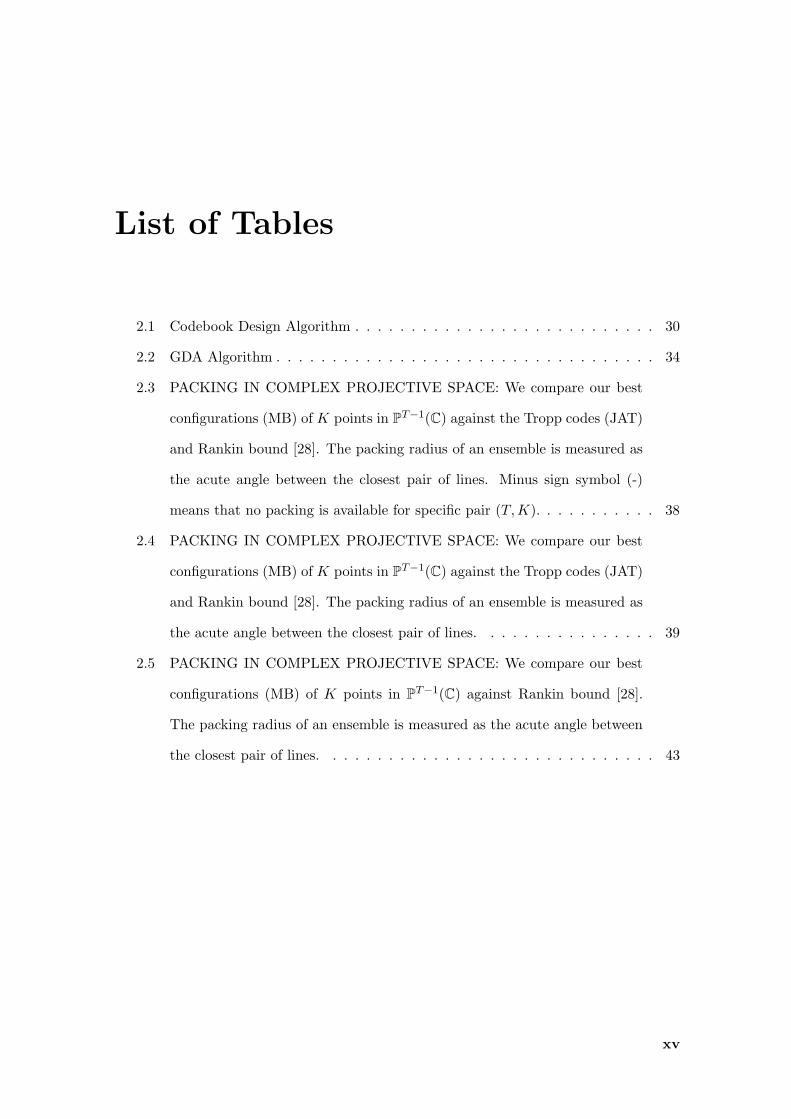
2.3 PACKING IN COMPLEX PROJECTIVE SPACE: We compare our best
configurations (MB) of K points in PT−1(C) against the Tropp codes (JAT)
and Rankin bound [28]. The packing radius of an ensemble is measured as
the acute angle between the closest pair of lines. Minus sign symbol (-)
means that no packing is available for specific pair (T, K). . . . . . . . . . . 38
2.4 PACKING IN COMPLEX PROJECTIVE SPACE: We compare our best
configurations (MB) of K points in PT−1(C) against the Tropp codes (JAT)
and Rankin bound [28]. The packing radius of an ensemble is measured as
the acute angle between the closest pair of lines. . . . . . . . . . . . . . . . 39
2.5 PACKING IN COMPLEX PROJECTIVE SPACE: We compare our best
configurations (MB) of K points in PT−1(C) against Rankin bound [28].
The packing radius of an ensemble is measured as the acute angle between
the closest pair of lines. . . . . . . . . . . . . . . . . . . . . . . . . . . . . . 43
xv

xvi LIST OF TABLES

Notation
For reference purposes, some of the most common symbols and acronyms used throughout
this thesis are listed below.
Symbols
[A]i,j the ij-th element of matrix A
A∗ the complex conjugate of A
AT the transpose of A
AH the conjugate transpose (Hermitian) of A
A−1 the inverse of A
A1
2 the Hermitian square root of the positive semidefinite matrix A
tr (A) the trace of A
det (A) the determinant of A
A⊗B the Kronecker product of A and B
AB the Schur-Hadamard product of A and B
rank (A) the rank of A
In the n× n identity matrix
0m×n the m× n zero matrix
1n the n-dimensional column vector with all entries equal to one
λmax(A) the maximum eigenvalue of Hermitian A
λmin(A) the minimum eigenvalue of Hermitian A
vec(A) the vector obtained by stacking the columns of A on top of each other, from
left to right
xvii

xviii Notation
‖A‖ the Frobenius norm; ‖A‖ =√
tr(AHA)
CN (µ,Σ) multivariate circularly symmetric, complex Gaussian distribution with mean
vector µ and covariance matrix Σ
N (µ,Σ) real-valued Gaussian distribution with mean vector µ and covariance matrix
Σ
P (A) the probability of the event A
Q(x) the Gaussian Q-function: if x∼N (0, 1), then P (x > t) = Q (t)
p(·) probability density function
o(x) if f(x) = o(x), then limx→0f(x)
x = 0
<· the real part
=· the imaginary part
A B the matrix A−B is positive semidefinite
d= equality in distribution
∼ distributed according to
loga x the base-a logarithm of x; when a is omitted it denotes the natural algorithm
of x
C the set of complex numbers
CN the set of N -dimensional complex vectors
CM×N the set of M ×N complex matrices
diag(A) the column vector obtained by extracting the diagonal elements of A
Ep[ · ] the expectation with respect to the probability density function p; p omitted
whenever no confusion can occur
i the imaginary unit; i =√−1
≈ approximately equal to
δij the Kronecker symbol; equal to one if i = j and zero otherwise
R the set of real numbers
RN the set of N -dimensional real vectors
RM×N the set of M ×N real matrices
xix
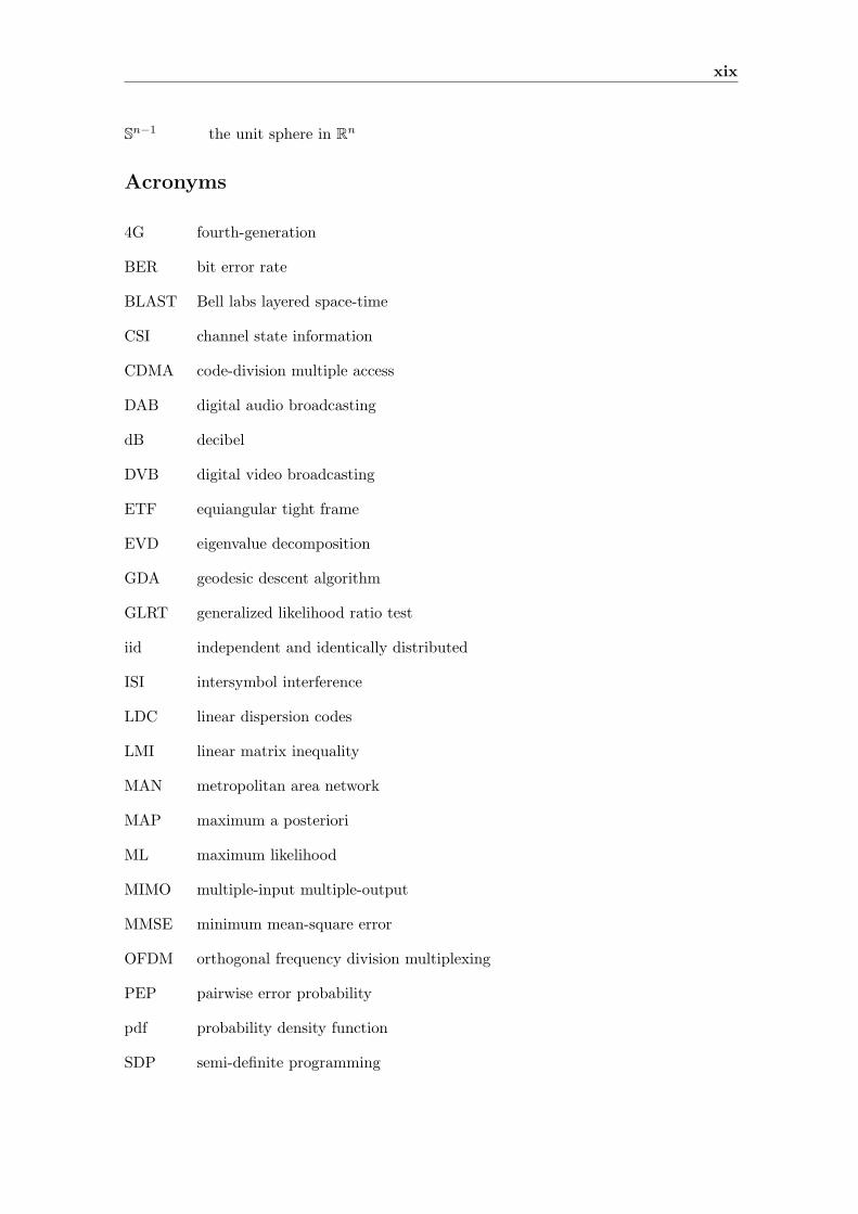
Sn−1 the unit sphere in R
n
Acronyms
4G fourth-generation
BER bit error rate
BLAST Bell labs layered space-time
CSI channel state information
CDMA code-division multiple access
DAB digital audio broadcasting
dB decibel
DVB digital video broadcasting
ETF equiangular tight frame
EVD eigenvalue decomposition
GDA geodesic descent algorithm
GLRT generalized likelihood ratio test
iid independent and identically distributed
ISI intersymbol interference
LDC linear dispersion codes
LMI linear matrix inequality
MAN metropolitan area network
MAP maximum a posteriori
ML maximum likelihood
MIMO multiple-input multiple-output
MMSE minimum mean-square error
OFDM orthogonal frequency division multiplexing
PEP pairwise error probability
pdf probability density function
SDP semi-definite programming

xx Notation
SER symbol error rate
SISO single-input single-output
SNR signal-to-noise ratio
SIC successive interference cancelation
SVD singular value decomposition
STC space-time codes
STBC space-time block codes
STTC space-time trellis codes
TDMA time-division multiple-access
UB union bound
WLAN wireless local area network
w.l.o.g. without loss of generality
w.r.t. with respect to

Chapter 1
Introduction
The demand for mobile communications systems with high data rates and improved link
quality for a variety of applications has dramatically increased in recent years. Although
the benefits of using multi-antenna receivers have been known for a long time, the di-
versity and rate gains attainable using multiple antennas at both transmit and receive
sides have been understood only recently. Winters [1] was among the first to prove that
multiple-input multiple-output (MIMO) systems can provide a capacity increase. Paulraj
and Kailath [2] demonstrated that the capacity of cellular code-division multiple access
(CDMA) systems equipped with multiple antennas at both transmit and receive sides can
increase considerably with respect to single-input single output (SISO) systems. Then
Telatar [3] proved the fundamental results on the capacity of flat-fading MIMO channels.
These results were independently derived and extended with practical considerations by
Foschini et al. [4]. The main finding of these information theoretic analyzes was that at
high signal-to-noise ratio (SNR) the capacity of multiple antenna channels increases lin-
early with the smaller of the number of transmit and receive antennas. This has led to
a great deal of research on space-time codes (STC) to exploit both spatial and temporal
diversity to maximize channel capacity. The key development of the STC was originally
revealed in [5] in the form of trellis codes, which required a multidimensional Viterbi al-
gorithm at the receiver for decoding. These codes, called space-time trellis codes (STTC),
provide a diversity gain equal to the number of transmit antennas in addition to a coding
gain that depends on the complexity of the code (i.e., number of states in the trellis) with-
out any loss in bandwidth efficiency. When the number of antennas is fixed, the decoding
1
2 Introduction
complexity of STTC (measured by the number of trellis states at the decoder) increases
exponentially as a function of the diversity level and transmission rate. In addressing
the issue of decoding complexity, Alamouti [6] discovered a remarkable space-time block
coding scheme for transmission with two antennas. This scheme supports maximum like-
lihood (ML) detection based on linear processing and scalar detection at the receiver. The
very simple structure and linear processing of the Alamouti construction makes it a very
attractive scheme that is currently part of wideband CDMA and CDMA-2000 standards.
Tarokh et al. [7], by using orthogonal designs to create analogs of the Alamouti codes
for more that two transmit antennas, laid down the theory of the space-time block codes
(STBC). Their aim was also ML decoding with only linear processing at the receiver,
and this is the function of the orthogonal structure. As the number of transmit antennas
increases, the data rate available with orthogonal designs becomes unattractive. Hence
the recent focus on nonorthogonal linear codes designs such as linear dispersion codes
(LDC) [8] and the Golden code [9]. Bell labs layered space-time (BLAST) codes [4] can be
regarded as a special class of STBC where streams of independent data are transmitted
over different antennas, thus maximizing the average data rate over the MIMO system.
There are various layered space-time architectures depending upon whether error control
coding is used or not and by the way modulated symbols are assigned to the transmit
antennas. Such architectures include the vertical [10], horizontal [11], diagonal [11] and
threaded layered space-time architectures [12]. In order to perform symbol detection, the
receiver must unmix he channel, in one of several possible ways. The complexity of ML
decoding can be high when many antennas or higher order modulations are used. En-
hanced variants of this like sphere decoding [13] have been proposed. Another popular
decoding strategy proposed along vertical BLAST is known as nulling and canceling which
resembles the successive interference cancelation (SIC) proposed for multiuser detection
in CDMA receivers [14]. While there are several receiver architectures that can support
the full degrees of freedom of the channel, nulling and canceling in combination with min-
imum mean-square error (MMSE) estimation achieves capacity. See, e.g., [15, Chapter 8]
for more details.
3
PSfrag replacements
X
1
M
Tx h1N
h11
h12
hM1
hMN
1
2
N
Rx Y
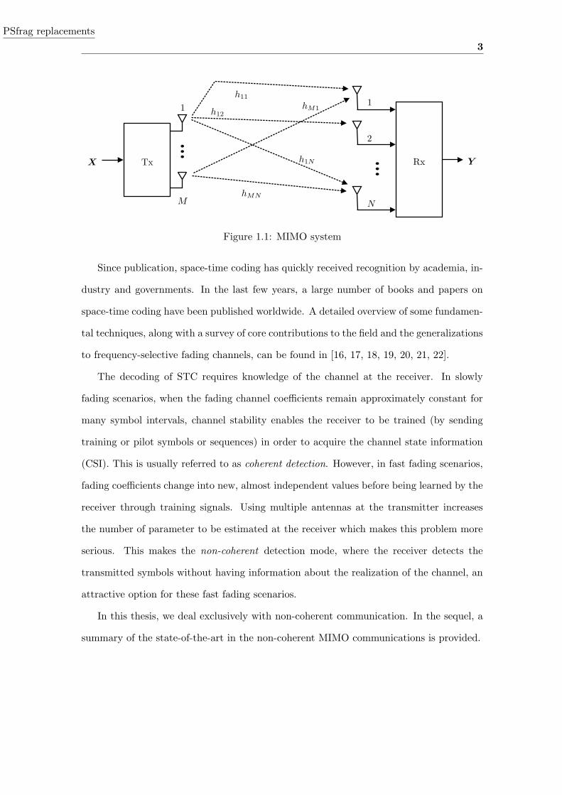
Figure 1.1: MIMO system
Since publication, space-time coding has quickly received recognition by academia, in-
dustry and governments. In the last few years, a large number of books and papers on
space-time coding have been published worldwide. A detailed overview of some fundamen-
tal techniques, along with a survey of core contributions to the field and the generalizations
to frequency-selective fading channels, can be found in [16, 17, 18, 19, 20, 21, 22].
The decoding of STC requires knowledge of the channel at the receiver. In slowly
fading scenarios, when the fading channel coefficients remain approximately constant for
many symbol intervals, channel stability enables the receiver to be trained (by sending
training or pilot symbols or sequences) in order to acquire the channel state information
(CSI). This is usually referred to as coherent detection. However, in fast fading scenarios,
fading coefficients change into new, almost independent values before being learned by the
receiver through training signals. Using multiple antennas at the transmitter increases
the number of parameter to be estimated at the receiver which makes this problem more
serious. This makes the non-coherent detection mode, where the receiver detects the
transmitted symbols without having information about the realization of the channel, an
attractive option for these fast fading scenarios.
In this thesis, we deal exclusively with non-coherent communication. In the sequel, a
summary of the state-of-the-art in the non-coherent MIMO communications is provided.

4 Introduction
1.1 Non-Coherent MIMO Communications
Previous work. The capacity of non-coherent multiple antenna systems was studied
in [23, 24]. Under the additive white observation Gaussian noise and Rayleigh channel
assumptions, it has been shown that the signal matrix that achieves capacity can be
written as S = ΦV , where Φ is an T × T isotropically distributed unitary matrix, and V
is an independent T ×M real, nonnegative, diagonal matrix1 with M and T denoting the
number of transmit antennas and the length of the coherence interval, respectively; also,
it has been proven that at high SNR, or when T is much bigger than M , capacity can be
achieved by using a constellation of unitary matrices as codebooks. Furthermore, in [25]
has been shown that, under the assumption of equal-energy codewords and high SNR,
scaled unitary codebooks optimize the union bound (UB) on the error probability. Hence,
at high SNR unitary constellations are optimal from both the capacity and symbol error
probability viewpoints. Optimal unitary constellations correspond to optimal packings in
Grassmann manifolds [26]. In [27, 28], a systematic method for designing unitary space-
time constellations was presented. In [29], Sloane’s algorithms [30] for producing sphere
packings in real Grassmannian space have been extended to complex Grassmannian space.
For a small number of transmit antennas, by using chordal distance as the design criterion,
the corresponding constellations improve on the bit error rate (BER) when compared with
the unitary space-time constellations presented in [27]. In [31] the problem of designing
signal constellations for the multiple antenna non-coherent Rayleigh fading channel has
been examined. The asymptotic UB on the probability of error has been considered,
which, consequently, gave rise to a different notion of distance on the Grassmann manifold.
By doing this, a method of iteratively designing signals, called successive updates, has
been introduced. The signals obtained therein are, in contrast to [27, 29], guaranteed
to achieve the full diversity order of the channel. In [32] a family of space-time codes
suited for non-coherent MIMO systems was presented. These codes use all the degrees
of freedom of the system, and they are constructed as codes on the Grassmann manifold
1In calling the oblong matrix V diagonal, it means that only the elements along its main diagonal may
be nonzero.

1.1 Non-Coherent MIMO Communications 5
by the exponential map. Recently, in [33, 34] some sub-optimal simplified decodings for
the class of unitary space-time codes obtained via the exponential map were presented.
In [37], the authors considered non-coherent communication over a frequency-flat MIMO
Rayleigh block-fading channel. Using a subspace perturbation analysis, an appropriate
metric for the distance between Grassmannian constellation points is determined, and a
greedy technique for designing constellations that resemble the isotropic distribution is
then proposed. The inherent geometric structure of these constellations is used to develop
a novel suboptimum detector. The performance of this detector is comparable to that
of the ML detector, but it requires less computational effort. An interested reader is
referred to, e.g., [18, Chapter 10], for a summary of the most quoted propositions in the
non-coherent MIMO literature.
Low SNR MIMO systems have recently attracted attention of scientific community.
One of the reasons stems from the fact that in the third-generation mobile data systems
almost 40% of geographical locations experience receiver SNR levels below 0 dB while
only less than 10% display levels above 10 dB. High SNR requirement, besides its low
power efficiency, cannot always be satisfied due to the power limitations in the mobile
device. Also, recent technological advances have led to the emergence of small, low-power,
and possibly mobile devices which, when deployed in large numbers, have the ability to
form an intelligent (sensor) network which can monitor large areas, detect the presence or
absence of targets, etc. This motivates the analysis and construction of communication
schemes which can cope with the low SNR regime. See [38, 39, 40] for a more thorough
discussion of this topic.
Low SNR MIMO systems when CSI is available at the receiver have been treated in [38].
The interplay of rate, bandwidth, and power is analyzed in the region of energy per bit
close to its minimum value. The scenario where no CSI is available at the receiver has
been considered in [41]. It has been shown that the optimal signaling at low SNR achieves
the same capacity as the known channel case for single transmit antenna systems. Verdu,
in [42], has shown that knowledge of the first and second derivatives of capacity at low SNR
give us insight on bandwidth and energy efficiency for signal transmission. More precisely,

6 Introduction
these quantities tell us how spectral efficiency grows with energy-per-bit. In [43], a for-
mula for the second-order expansion of the input-output mutual information at low SNR
is obtained, whereas in [44] the capacity and the reliability function as the peak constraint
tends to zero are considered for a discrete-time memoryless channel with peak constrained
inputs. Similar results to [43, 44] have been obtained in [45] under weaker assumptions on
the input signals. In the same work, Rao and Hassibi have demonstrated that the on-off
signaling presented in [41] generalizes to the multi-antenna setting and attains the known
channel capacity. The tradeoff between communication rate and average probability of
decoding error using a framework of error-exponent theory has been investigated in [46].
It is argued that the advantage of having multiple antennas is best realized when the
fading is fully correlated, i.e., a performance gain of MN and a peakiness gain of M 2NT
can be achieved where M , N and T represent the number of transmit, receive antennas,
and the length of the coherence interval, respectively. The symbol error probability point
of view for the analysis of low SNR non-coherent independent and identically distributed
(iid) Rayleigh channel is more recent, although, Hochwald, et al. [27] had reported that in
the low SNR and Rayleigh fading channel it seems one should employ only one transmit
antenna. Borran et al. [39], under the assumption of equally probable codewords, pre-
sented a technique that uses Kullback-Liebler divergence between the probability density
functions induced at the receiver by distinct transmitted codewords as a design criterion
for codebook design. In low SNR condition, their constellation points occupy multiple
level (signal points lie in concentric spheres) with a point usually in the origin. The codes
thereby constructed were shown to perform better than some existing non-coherent code-
book constructions in low SNR, namely [27]. Srinivasan, et al. [47], considered the case of
single transmit antenna in the low SNR regime. Using the information theoretic results
over the low SNR non-coherent iid Rayleigh fading channel under an average power con-
straint (c.f. [45, 46]), they allow for codewords with unequal priors in a code and optimize
over prior probabilities to achieve better performance. This results in constellations that
assume a point in the origin with probability 12 , with the probabilities of the points lying
in the sphere being equal. In [48], the correlated Rayleigh fading model was studied and it

1.2 Thesis Outline and Contributions 7
was shown that at any SNR, any single antenna performs better when used with suitable
precoding in a MIMO correlated Rayleigh fading than in a single-input multiple output
SIMO channel. Consequently, code designs that exploit the correlations in the transmit
antennas in the MIMO case to provide gains over the corresponding SIMO case in the low
SNR regime were presented.
In the sequel, the motivation for the research presented in this thesis is discussed.
Motivation. The techniques aforementioned can not be readily extended to the more
realistic and challenging scenario, where the Gaussian observation noise has an arbitrary
correlation structure. The assumption of spatio-temporal Gaussian observation noise is
common, as there are at least two reasons for making it. First, it yields mathematical
expressions that are relatively easy to deal with. Second, in some scenarios it can be
justified via the central limit theorem. Although customary, the assumption of spatio-
temporal white Gaussian observation noise is clearly an approximation. In general, in
realistic scenarios, the noise term might have very rich correlation structure, e.g, see
pp. 554 in [15], pp. 100 in [18], pp. 10, 159, 171 in [19] and [38]. The generalization to
arbitrary noise covariance matrices encompasses many scenarios of interest as special cases:
spatially colored or not jointly with temporally colored or not observation noise, multiuser
environment, etc. Intuitively, unitary space-time constellations are not the optimal ones
for this scenario.
1.2 Thesis Outline and Contributions
The thesis is divided into 4 chapters. We summarize the content of each chapter, besides
the current one which gives the motivation and outline of this dissertation. For each
chapter, we also refer the publications (conference and journal papers) that it has given
rise.
In more detail, the outline of this thesis is as follows.

8 Introduction
1.2.1 Chapter 2
In Chapter 2, the problem of space-time codebook design for non-coherent communications
in multiple-antenna wireless systems and high SNR regime is addressed. In this work, we
look for a more practical code design criterion based on error probability, rather than
capacity analysis. The calculus of the exact expression for the average error probability
for the general non-coherent systems seems not to be tractable. Instead, we consider
pairwise error probability (PEP) in high SNR regime, and use it to find a code design
criterion (a merit function) for an arbitrarily given noise correlation structure.
Contribution. Our contributions in this area are summarized in the following:
1. The main contribution of this chapter is a new technique that systematically designs
space-time codebooks for non-coherent multiple-antenna communication systems.
In contrast with other approaches, the channel matrix is modeled as an unknown
deterministic parameter at both the receiver and the transmitter, and the Gaussian
observation noise is allowed to have an arbitrary correlation structure, known by the
transmitter and the receiver. In general correlated noise environments, computer
simulations show that the space-time codes obtained with our method significantly
outperform those already known which were constructed for spatio-temporally white
noise case. We recall that codebook constructions for arbitrary noise correlation
structures were not previously available and this demonstrates the interest of the
codebook design methodology introduced herein.
2. For the special case of spatio-temporal white observation noise, our codebooks re-
cover the previously known unitary structure, namely the codes in [27] (in fact, our
codes are marginally better). Also, for this specific scenario and M = 1 we show that
the problem of finding good codes coincides with the very well known packing prob-
lem in the complex projective space. We compare our best configurations against
the codes in [28] and the Rankin bound. We manage to improve the best known
results and in some cases actually provide optimal packings in complex projective
spaces which attain the Rankin upper bound.
1.2 Thesis Outline and Contributions 9
3. Theoretical analysis leading to an upper bound on PEP in the high SNR scenario
for the Gaussian observation noise with an arbitrary correlation structure.
Publications. The results of this work have been published in
M. Beko, J. Xavier and V. Barroso, “Codebook design for non-coherent communication
in multiple-antenna systems,” in Proc. of IEEE International Conference on Acoustics,
Speech, and Signal Processing (ICASSP), Toulouse, France, 2006.
as well in the form of a journal paper in
M. Beko, J. Xavier and V. Barroso, “Non-coherent Communication in Multiple-Antenna
Systems: Receiver design and Codebook construction,” IEEE Transactions on Signal
Processing , vol. 55, no. 12, pp. 5703 - 5715, Dec. 2007.
1.2.2 Chapter 3
In Chapter 3, we study the non-coherent MIMO channel in the low SNR regime from the
capacity and PEP viewpoints. The novel aspect is that we allow the Gaussian observation
noise to have an arbitrary correlation structure, albeit known to the transmitter and the
receiver.
Contribution. In the following, we summarize our contributions in this area:
1. The spatially correlated non-coherent MIMO block Rayleigh fading channel is an-
alyzed. This extends the approach in [45] as we take into account both channel
and noise correlation. The impact of channel and noise correlation on the mutual
information is obtained for the on-off and Gaussian signaling. The main conclusion
is that mutual information is maximized when both the transmit and receive anten-
nas are fully correlated. This shows that MIMO systems can actually be beneficial
in the low SNR regime. We also argue that the on-off signaling is optimal for this
multi-antenna setting.
2. Contrary to most approaches for the low SNR regime, the channel matrix is as-
sumed deterministic, i.e., no stochastic model is attached to it. A low SNR analysis
10 Introduction
of the PEP for the GLRT receiver is introduced, and a codebook design criterion
which takes into account the information about noise correlation is obtained. For the
special case of single transmit antenna and spatio-temporal white Gaussian noise,
it is shown that the problem of finding good codes corresponds to the very well
known packing problem in the complex projective space [28]. New space-time con-
stellations for some particular wireless scenarios are constructed. We argue that
one should construct codebooks for just one transmit antenna that match the noise
statistics. Computer simulations show that these new codebooks are also of interest
for Bayesian receivers which decode constellations with non-uniform priors.
Publications. The material contained in this chapter has been published in
M. Beko, J. Xavier and V. Barroso, “Codebook design for the non-coherent GLRT
receiver and low SNR MIMO block fading channel,” in Proc. of IEEE Workshop on Signal
Processing Advances in Wireless Communications (SPAWC), Cannes, France, 2006.
M. Beko, J. Xavier and V. Barroso, “Capacity and error probability analysis of non-
coherent MIMO systems in the low SNR regime,” in Proc. of IEEE International Confer-
ence on Acoustics, Speech, and Signal Processing (ICASSP), Honolulu, HI USA, 2007.
In addition, a journal paper extending the previous results was submitted as
M. Beko, J. Xavier and V. Barroso, “Further results on the capacity and error prob-
ability analysis of non-coherent MIMO systems in the low SNR regime,” accepted for
publication in IEEE Transactions on Signal Processing.
1.2.3 Chapter 4
This chapter concludes the thesis summarizing the main obtained results and enumerating
the future lines of work.

Chapter 2
Receiver Design and Codebook
Construction in the High SNR
Regime
2.1 Chapter Summary
The chapter is organized as follows. In section 2.2, we introduce the data model and formu-
late the problem addressed in this chapter. We describe the structure of our non-coherent
receiver and discuss the selection of the codebook design criterion. In section 2.3, before
addressing the codebook design problem we draw some conclusions about the design crite-
rion defined in section 2.2. In section 2.4, we propose a new algorithm that systematically
designs non-coherent space-time constellations for an arbitrarily given noise covariance
matrix and any M , N , K and T , respectively, number of transmitter antennas, number
of receiver antennas, size of codebook, and channel coherence interval. In section 2.5,
we present codebook constructions for several important special cases and compare their
performance with state-of-art solutions. Section 2.6 presents the main conclusions of this
chapter.
2.2 Problem Formulation
Data model and assumptions. The communication system comprises M transmit
and N receive antennas and we assume a block flat fading channel model with coherence
interval T . That is, we assume that the fading coefficients remain constant during blocks
of T consecutive symbol intervals, and change into new, independent values at the end
11

12 Receiver Design and Codebook Construction in the High SNR Regime
of each block. It is an accurate representation of many time-division multiple-access
(TDMA), frequency-hoping, or block-interleaved systems. See, e.g., [27] for more details.
In complex base band notation we have the model
Y = XHH + E, (2.1)
where X is the T ×M matrix of transmitted symbols (the matrix X is called hereafter
a space-time codeword), Y is the T × N matrix of received symbols, HH is the M × N
matrix of channel coefficients (the operator H is used for the sake of convenience), and
E is the T × N matrix of zero-mean additive observation noise. In Y , time indexes the
rows and space (receive antennas) indexes the columns. We shall work under the following
assumptions:
A1. (Channel matrix) The matrix H is not known at the receiver neither at the
transmitter, and no stochastic model is assumed for it;
A2. (Transmit power constraint) The codeword X is chosen from a finite codebook
C = X1, X2, . . . , XK known to the receiver, where K is the size of the codebook.
We impose the power constraint tr(XHk Xk) = 1 for each codeword. Furthermore,
we assume that T ≥ M and each codeword is of full rank, i.e., rank(X) = M ;
A3. (Noise distribution) The observation noise at the receiver is zero mean and obeys
circular complex Gaussian statistics, that is, vec(E) ∼ CN (0,Υ). The noise covari-
ance matrix Υ = E[vec(E)vec(E)H ] is known at the transmitter and at the receiver
(vec(E) stacks all columns of the matrix E on the top of each other, from left to
right).
Remark that in assumption A3, we let the data model depart from the customary
assumption of spatio-temporal white Gaussian observation noise. Also, note that one
cannot perform “pre-whitening” in order to revert the colored case (Υ 6= ITN ) into the
spatio-temporal white noise case (Υ = ITN ). To see this, let’s consider two systems where
system 1 is described by
Y 1 = X1HH + E1, (2.2)

2.2 Problem Formulation 13
with e1 = vec(E1) ∼ CN (0,Υ), and system 2 is given by
Y 2 = X2HH + E2, (2.3)
with e2 = vec(E2) ∼ CN (0, ITN ). The systems (2.2) and (2.3) are equivalent to
y1 = vec(Y 1) = (IN ⊗X1) vec(HH) + e1, (2.4)
y2 = vec(Y 2) = (IN ⊗X2) vec(HH) + e2 (2.5)
respectively (the symbol⊗ denotes the Kronecker product). After pre-whitening, from (2.4)
we get
y1 = Υ− 1
2 y1 = Υ− 1
2 (IN ⊗X1) vec(HH) + e1 (2.6)
with e1 = Υ− 1
2 e1 ∼ CN (0, ITN ). From (2.5) and (2.6) we deduce that the systems 1
and 2 are not equivalent, i.e., the unitary constellations (which are optimal for spatio-
temporally white noise at high SNR) cannot be employed by performing suitable pre-
whitening because it breaks down the structure of the constellation. A more detailed
discussion on this point can be found in subsection 2.2.1 .
Receiver. According to the system model (2.1) and the assumptions above mentioned,
the conditional probability density function (pdf) of the received vector y = vec(Y ), given
the transmitted matrix X and the unknown realization of the channel g = vec(HH
), is
given by
p(y|X, g) =exp−||y − (IN ⊗X)g||2
Υ−1
πTNdet(Υ),
where the notation ||z||2A = zHAz was used.
Since no stochastic model is attached to the channel propagation matrix, the receiver
faces a multiple hypothesis testing problem with the channel H as a deterministic nuisance
parameter. We assume a generalized likelihood ratio test (GLRT) receiver which decides
the index k of the codeword as the index k such that
k = argmax p(y|Xk, gk)k = 1, 2, . . . , K
= argmin∥∥∥y − Xkgk
∥∥∥2
Υ−1
k = 1, 2, . . . , K

14 Receiver Design and Codebook Construction in the High SNR Regime
where
Xk = IN ⊗Xk and gk = (X Hk X k)
−1X Hk Υ− 1
2 y (2.7)
with X k = Υ− 1
2 Xk denoting the whitened version of Xk . The GLRT [49, 50, 51] is
composed of a bank of K parallel processors where the k -th processor assumes the presence
of the k -th codeword and computes the likelihood of the observation, after replacing the
channel by its ML estimate. The GLRT detector chooses the codeword associated with
the processor exhibiting the largest likelihood of the observation. We note that the GLRT
performs sub-optimally when compared with the ML receiver, as the latter can exploit
the knowledge of channel statistics’. However, since assumption A1 is in force, the GLRT
yields an attractive (implementable) solution in the present setup. Note also that, for the
special case of unitary constellations, i.e., XHk Xk = 1
M IM for all k, spatio-temporal white
Gaussian noise and iid Rayleigh fading, it is readily shown that the two receivers coincide.
Due to the respective expression for the ML estimate of the channel, equation (2.7), we
note that since each codeword of the codebook has full rank (assumption A2), the channel
estimate is well defined.
Codebook design criterion. In this chapter, our goal is to design a codebook C =
X1, X2, . . . , XK of size K for the current setup. A codebook C is a point in the space
M = (X1, . . . , XK) : tr(XHk Xk) = 1.
Note that the spaceM can be viewed as multi-dimensional torus, i.e, the Cartesian product
of K unit-spheres :
M = S2TM−1 × · · · × S
2TM−1 (K times)
and each codeword Xk belongs to CT×M . The symbol S
n−1 denotes the unit sphere in
Rn. First, we must adopt a merit function f : M→ R which gauges the quality of each
constellation C. The average error probability for a specific C would be the natural choice,
but the theoretical analysis seems to be intractable. Instead, as usual [24]- [27], we rely on
a PEP study to construct our merit function. For the special case of unitary codebooks
(XHk Xk = 1
M IM ), spatio-temporal white Gaussian noise (Υ = ITN ) and iid Rayleigh
2.2 Problem Formulation 15
fading, the exact expression and Chernoff upper bound for the PEP have been derived in
[24]. However, the calculus of these expressions for the general case, i.e, arbitrary matrix
constellations C and noise correlation matrix Υ, seems to be burdensome. As in [24]- [27],
in this chapter, we focus on the high SNR regime. Namely, we resort to the asymptotic
expression of the PEP in the high SNR regime, for arbitrary C and Υ. To start the
PEP analysis, we consider a codebook with only two codewords, i.e., C = X1, X2. Let
PXi→Xjbe the probability of the GLRT receiver deciding X j when X i is sent. It can be
shown (see Appendix A) that at sufficiently high SNR we have the approximation
PXi→Xj≈ Q
(1√2
√gH Lijg
), (2.8)
with
Lij = X Hi Π⊥
j X i and Π⊥j = ITN −X j
(X H
j X j
)−1X H
j
where Q(x) =∫ +∞x
1√2π
e−t2
2 dt is the Q-function and Π⊥j is the orthogonal projector onto
the orthogonal complement of the column space of X j .
Equation (2.8) shows that the probability of misdetecting X i for Xj , depends on the
channel realization g = vec(HH
)and on the relative geometry of the codewords X i and
X j . We can decouple the action of g and Lij as follows: using the inequality
gHLijg ≥ λmin(Lij) ||g||2,
which is an equality when M = 1 and Υ = INT , and the fact that Q(·) is monotonically
non-increasing, we have the upper bound on the PEP for high SNR
PXi→Xj≤ Q
(1√2||g||
√λmin(Lij)
). (2.9)
We cannot control the power of the channel g = vec(HH), but we can design codebooks
aiming at maximizing λmin(Lij). We see that, if M = 1 and Υ = INT , the bound in (2.9)
is attained for arbitrary C.
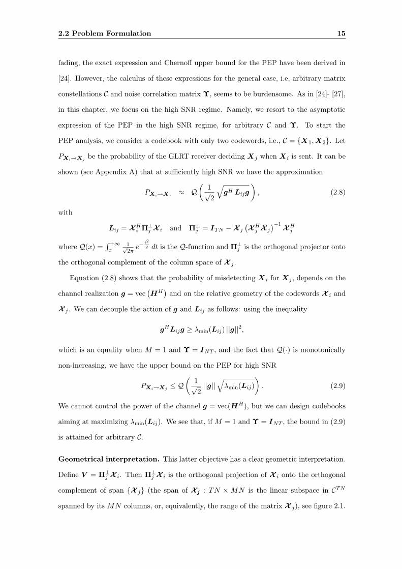
Geometrical interpretation. This latter objective has a clear geometric interpretation.
Define V = Π⊥j X i. Then Π⊥
j X i is the orthogonal projection of X i onto the orthogonal
complement of span X j (the span of Xj : TN × MN is the linear subspace in CTN
spanned by its MN columns, or, equivalently, the range of the matrix X j), see figure 2.1.

16 Receiver Design and Codebook Construction in the High SNR Regime
PSfrag replacements
Π⊥j X i
X j
X i
Figure 2.1: Geometrical interpretation of Π⊥j X i.
Now, note that
Lij = V HV = (Π⊥j X i)
H(Π⊥j X i)
is the corresponding Gram matrix and
√det(V HV ) =
√λmin(V
HV ) · . . . · λmax(VHV ) ≥ λmin(V
HV )MN
2 .
Hence, by maximizing λmin(VHV ), we are increasing a lower bound on
√det(V HV
)
which is proportional to the volume of the parallelepiped spanned by the columns of the
Π⊥j X i. That is, we are trying to place X i in the orthogonal complement of span X j.
Problem formulation. Following a worst-case approach, we are led from (2.9) to define
the codebook merit function
f : M→ R and C = X1, . . . , XK 7→ f(C)
as
f(C) = minfij(C) : 1 ≤ i 6= j ≤ K (2.10)
2.2 Problem Formulation 17
where fij(C) = λmin(Lij(C)). Constructing an optimal codebook C = X1, X2, ..., XK
amounts to solving the optimization problem
C∗ = arg maxC ∈ M
f(C). (2.11)
The problem defined in (2.11) is a high-dimensional, non-linear and non-smooth optimiza-
tion problem. As an example, for a codebook of size K = 256 the number of fij functions
is K(K − 1) = 65280. Also, for T = 8 and M = 2, there are 2KTM = 8192 real variables
to optimize.
The problem in (2.11) is a non-smooth optimization problem because the objective
function f , as the pointwise minimum of several fij ’s, is in general not smooth at points
where the minimum is attained by several f ′ijs. In our case, each fij is not even smooth,
due to the λmin operator. For an illustrative example, consider φ : R → R,
φ(t) = λmin
([t 00 −t
]).
Although the matrix involved is a smooth function of its entries, φ(t) = −|t| is not smooth
everywhere. Moreover, note that we have
f(X1, X2, . . . , XK) = f(X1eiθ1 , X2e
iθ2 , . . . , XKeiθK )
for any θk ∈ R and k = 1, . . . , K. This means that f depends on each Xk (‖Xk‖ = 1)
only through the line spanned by it (i.e., λXk : λ ∈ C).
2.2.1 A Note on Pre-Whitening
It may not be immediately obvious why the “pre-whitening” device cannot be employed
here. After all, this is a common trick in signal processing for generalizing solutions
formulated for white noise to the colored noise setup. However, since it cannot be done in
our situation, in the sequel, we try to provide more detailed explanations.
(i) As pointed out, “pre-whitening” cannot be performed as it changes the constella-
tion’s structure. Essentially, this summarizes our argument in equations (2.2)-(2.6). We
will now furnish another viewpoint on this matter.
18 Receiver Design and Codebook Construction in the High SNR Regime
When one asks if “pre-whitening” can be performed, one is asking if the solution to
the white noise case can be “transported” to the colored case. That is, one is asking if
the codebook construction problem for the colored case has an equivalent reformulation
in the white noise setup. Of course, if this were true, then it would be sufficient to have a
tool to construct codebooks for the white noise case, say, our tool solving the optimization
problem stated in equation (2.11) for the white noise case. We argue that, in our situation,
we cannot find such an equivalent reformulation.
To demonstrate our claim, consider the special case M = 1 (single transmit antenna),
N = 1 (single receive antenna) and T ≥ 2. As mentioned above, suppose that a tool is
available to solve problem (2.11) for the white noise case Υ = IT . Denoting codebooks
by
C = [x1 x2 · · · xK ] : T ×K
(each xk is a codeword) this means precisely that we have a tool to solve the optimization
problem (for any chosen T and K)
P1 : max
diag(CHC
)= 1T
fIT(C)
where 1T = (1, 1, . . . , 1)T (T times), diag(A) extracts the diagonal of matrix A and, for
any positive-definite T × T matrix Σ, we use the notation
fΣ(C) = min
xHi Σ−1xi − xH
i Σ−1xj
(xH
j Σ−1xj
)−1xH
j Σ−1xi : i 6= j
.
Now, solving the codebook construction problem (2.11) for a general noise correlation
matrix Υ corresponds to solving the optimization problem
P2 : max
diag(CHC
)= 1T
fΥ(C).
We now try reformulate problem P2 into the format P1. We start by noticing that we
have the identity
fΥ(C) = fIT
(Υ−1/2C
).

2.2 Problem Formulation 19
Thus, problem P2 is equivalent, through the change-of-variables D = Υ−1/2C (“pre-
whitening”), to the problem
P3 : max
diag(DHΥC
)= 1T
fIT(D).
The solution of problem P3 cannot be extracted from the one in problem P1. Note
that both problems have the same objective function but, whereas problem P1 searches
the codewords over a unit-sphere, problem P3 searches them over an ellipsoid. This is a
different problem.
Just as a side remark, note that a similar phenomenon (problems became inequivalent
as a unit-sphere constraint is changed to an ellipsoidal one) occurs when one tries to
project a point x0 ∈ Rn onto a sphere or onto an ellipsoid, i.e.,
Pa : minxT x = 1
1
2‖x− x0‖2 Pb : min
xT Ax = 1
1
2‖x− x0‖2
where A : n×n is positive-definite. It is well known that problem Pb cannot be reformu-
lated as problem Pa: it is known that Pb does not admit a closed-form solution, whereas
Pa does (radial projection).
The above argument used our tool but this is not restrictive: the key-point here is
that “pre-whitening” the data model changes the power constraints (which constitute an
important part of the problem formulation) and therefore changes the structure of the
optimal constellation.
(ii) To address further this question we reproduce here equations (2.4) and (2.6)
y1 = vec(Y 1) = (IN ⊗X1) vec(HH) + e1
y1 = Υ− 1
2 y1 = Υ− 1
2 (IN ⊗X1) vec(HH) + e1
where y1 corresponds to a colored noise system (e1 ∼ CN(0,Υ)) and y1 represents the
“pre-whitened” system (e1 ∼ CN (0, INT )). We recall that a white noise system corre-
sponds to equation (2.5), i.e.,
y2 = vec(Y 2) = (IN ⊗X2) vec(HH) + e2

20 Receiver Design and Codebook Construction in the High SNR Regime
where e2 ∼ CN (0, INT ). We have a solution for model y2 (reference [27]). We want to use
it in the model y1. However, the structure of the model y1 matches the structure of the
model y2 if and only if (iff) the signal Υ−1/2 (IN ⊗X1) can be put in the block-diagonal
format IN ⊗X2. This is possible iff Υ has the special structure
Υ = IN ⊗Σ
(from a physical viewpoint, corresponds to spatially uncorrelated receive antennas). Thus,
for general Υ, we cannot “transport” a solution obtained for the data model y2 to the
data model y1. But, let’s address the special case Υ = IN ⊗Σ. We would have
y1 =(IN ⊗
(Σ− 1
2 X1
))vec(HH) + e1.
Now, the codebook construction solution provided in [27] for the data model y2 consists
in selecting X2 from unitary constellations. Employing this solution in the data model y1
corresponds to making Σ−1/2X1 unitary. That is, suppose C = U 1, . . . , UK (UHk Uk =
1M IM ) is an optimal unitary codebook for y2, i.e., the codeword X2 is selected within C.
Then, with respect to the data model y1 one should take Σ−1/2X1 ∈ C, or, equivalently,
the codeword X1 should be taken from
C =Σ1/2U1, . . . ,Σ
1/2UK
.
The main problem is here is that the codebook C does not verify the power constraint,
i.e., in general, we will not have
tr(UH
k ΣUk
)= 1 for all k = 1, 2, . . . , K
for generic unitary matrices U k. One (sub-optimal) way around this is to enforce the
power constraint and pass to the codebook
C =
Σ1/2U1∥∥∥Σ1/2U1
∥∥∥, . . . ,
Σ1/2UK∥∥∥Σ1/2UK
∥∥∥
. (2.12)
Another way around is to define the following codebook
C =Σ1/2V 1,ΘΣ1/2V 1, . . . ,Θ
K−1Σ1/2V 1
(2.13)

2.2 Problem Formulation 21
where the T × M matrix V 1 is such that V H1 V 1 = 1
M IM and tr(V H1 ΣV 1) = 1. The
matrix Θ is a T × T diagonal matrix whose diagonal elements are ei2πu1/K ,...,ei2πuT /K
with the coefficients u1,...,uT presented in [27]. Note that Θ is a unitary matrix and that
ΘK = IT . Clearly, the codebook C satisfies the power constraint in the assumption A2.
We emphasize that C and C were heuristically obtained (do not satisfy an optimal-
ity criterion). Their performance will be assessed by a computer simulation, please see
figures 2.7-2.9 in section 2.5.
(iii) Under the assumption A1, no statistical model is attached to the channel matrix.
Anyhow, we present an analysis for the case when vec(H) ∼ CN (0, IMN ). Due to the
assumption A3, vec(E) ∼ CN (0,Υ) for some Υ 0. We start by remarking that the
model in (2.1) can be rewritten as
Y H = HXH + EH ,
and hence as
y = Gx + e, (2.14)
where y = vec(Y H), x = vec(XH), e = vec(EH) and G = IT ⊗H. From the perspective
of most communications objectives, the system described in (2.14) is equivalent to the
system
y = Gx + e, (2.15)
where e ∼ CN (0, ITN ), and
G = L−1G, (2.16)
where L is a Cholesky factor of Υ; i.e., Υ = LLH . This represents the channel model
in which the first step of the receiver processing is to pre-whiten the noise. It is clear
from (2.16) that the statistics of the elements of G are different from those of G and,
hence, unitary constellations cannot be employed.

22 Receiver Design and Codebook Construction in the High SNR Regime
2.3 Considerations About the New Codebook Merit Func-
tion
Before addressing the codebook design problem (2.10) we draw in this section some con-
clusions about the codebook merit function f in (2.10). In subsection 2.3.1, we show that,
for the special case of spatio-temporally white noise and K = 2, the unitary constellations
are the optimal ones with respect to f . In subsection 2.3.2, we show that, when restricting
attention to unitary codebooks, our codebook design criterion corresponds to a packing
problem in the Grassmannian space with respect to spectral distance, for the white noise
case. In subsection 2.3.3, we argue that the design method proposed in (2.11) guarantees
that the constructed constellation has full diversity when T ≥ 2M .
2.3.1 Optimality of Unitary Codewords for the White Noise Case
Consider a codebook with two codewords C = X1, X2. We want to maximize f(C) =
minλmin(Lij(C)) : i 6= j subject to tr(XH
k Xk
)= 1. We rewrite Lij(C) as
Lij(C) =(X H
i X i
) 1
2(IMN −UH
i U jUHj U i
) (X H
i X i
) 1
2 (2.17)
where U i = X i
(X H
i X i
)− 1
2 , U j = X j
(X H
j X j
)− 1
2 . That is, U i contains an orthonormal
basis for the subspace spanned by the columns of X i. Notice that UHj U j = UH
i U i = IMN .
To proceed with the analysis we use an useful fact from the cosine sine (CS) decomposition,
see [52] pp. 199: if U i, U j are TN ×MN matrices with orthonormal columns (T ≥ M),
then there exist MN × MN unitary matrices W 1 and W 2, and a TN × TN unitary
matrix Q with the following properties:
(i) If 2MN ≤ TN (2M ≤ T ), then
QU iW 1 =
IMN
0MN
0(TN−2MN)×MN
, QU jW 2 =
Cij
Sij
0(TN−2MN)×MN
(2.18)
where Cij is a diagonal MN × MN matrix with diagonal entries cos α1, . . . , cosαMN ,
0 ≤α1≤. . .≤αMN≤ π2 , and S2
ij + C2ij = IMN . Now, using (2.18) we can write
W H2 UH
j QHQU iW 1 = W H2 UH
j U iW 1 = Cij ⇒ UHj U i = W 2CijW
H1 , (2.19)
2.3 Considerations About the New Codebook Merit Function 23
so αi for i = 1, . . . , MN are the principal angles between the subspaces spanned by U i
and U j . Due to Ostrowski’s theorem pp. 224, 225 in [53], and equations (2.17) and (2.19),
it is not difficult to see that the following inequality holds
λmin (Lij) ≥ λmin
(X H
i X i
)λmin
(S2
ij
). (2.20)
Clearly, from (2.20), we deduce that in order to minimize an upper bound on PEP in high
SNR regime, one should simultaneously increase λmin
(X H
i X i
)and λmin
(S2
ij
). Unfortu-
nately, the right-hand side of the inequality (2.20) does not offer much insight into the form
of the optimal codebook for the case of arbitrary noise covariance matrix Υ (even for the
case K = 2). One of the reasons originates from the fact that pairwise error probabilities
are not symmetric for this general case. Hence, in the following, we treat the specific case
of spatio-temporal white Gaussian observation noise to find out what conclusions can we
draw about the form of the optimal codebook.
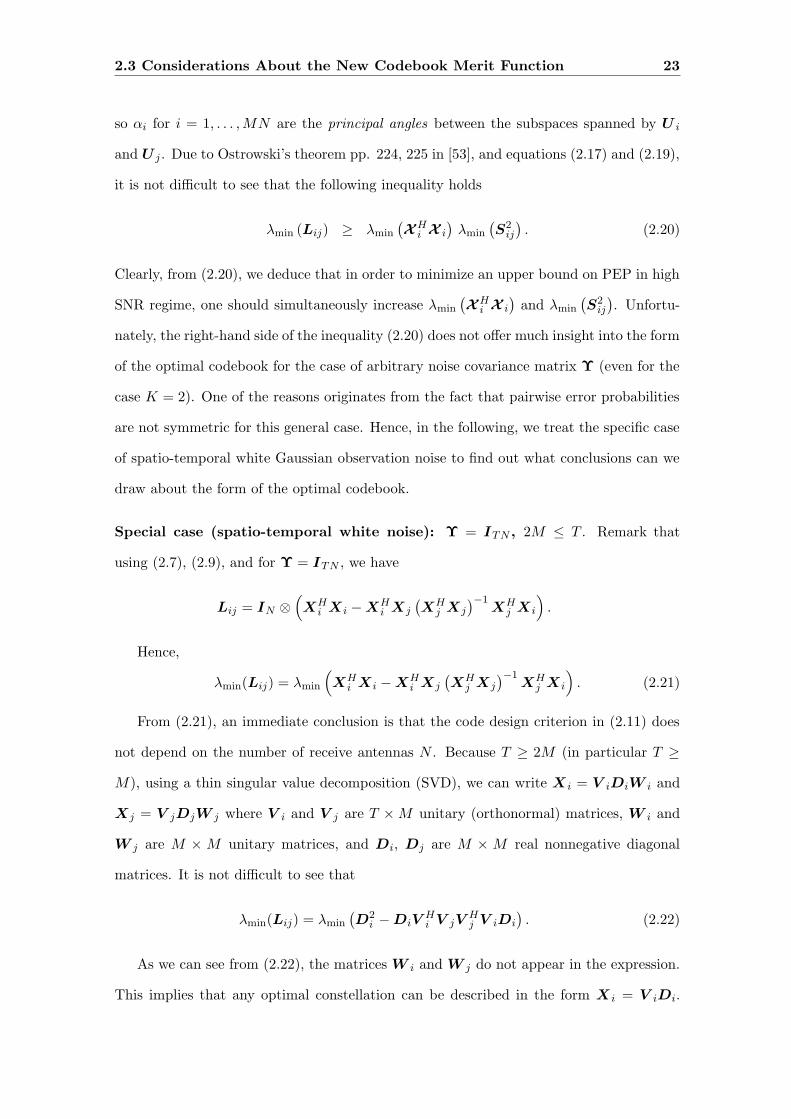
Special case (spatio-temporal white noise): Υ = ITN , 2M ≤ T . Remark that
using (2.7), (2.9), and for Υ = ITN , we have
Lij = IN ⊗(XH
i Xi −XHi Xj
(XH
j Xj
)−1XH
j Xi
).
Hence,
λmin(Lij) = λmin
(XH
i Xi −XHi Xj
(XH
j Xj
)−1XH
j Xi
). (2.21)
From (2.21), an immediate conclusion is that the code design criterion in (2.11) does
not depend on the number of receive antennas N . Because T ≥ 2M (in particular T ≥
M), using a thin singular value decomposition (SVD), we can write X i = V iDiW i and
Xj = V jDjW j where V i and V j are T ×M unitary (orthonormal) matrices, W i and
W j are M × M unitary matrices, and Di, Dj are M × M real nonnegative diagonal
matrices. It is not difficult to see that
λmin(Lij) = λmin
(D2
i −DiVHi V jV
Hj V iDi
). (2.22)
As we can see from (2.22), the matrices W i and W j do not appear in the expression.
This implies that any optimal constellation can be described in the form X i = V iDi.
24 Receiver Design and Codebook Construction in the High SNR Regime
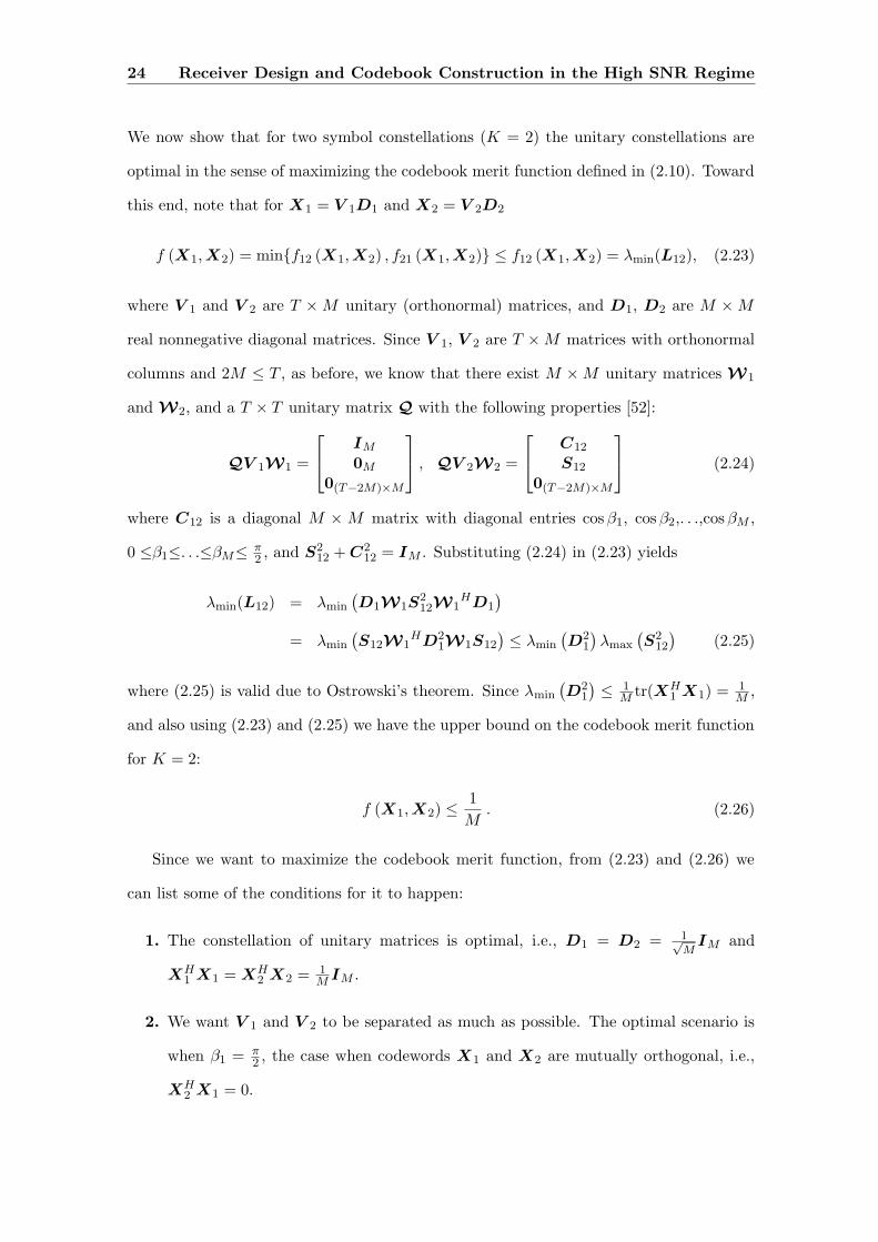
We now show that for two symbol constellations (K = 2) the unitary constellations are
optimal in the sense of maximizing the codebook merit function defined in (2.10). Toward
this end, note that for X1 = V 1D1 and X2 = V 2D2
f (X1, X2) = minf12 (X1, X2) , f21 (X1, X2) ≤ f12 (X1, X2) = λmin(L12), (2.23)
where V 1 and V 2 are T ×M unitary (orthonormal) matrices, and D1, D2 are M ×M
real nonnegative diagonal matrices. Since V 1, V 2 are T ×M matrices with orthonormal
columns and 2M ≤ T , as before, we know that there exist M ×M unitary matrices W1
and W2, and a T × T unitary matrix Q with the following properties [52]:
QV 1W1 =
IM
0M
0(T−2M)×M
, QV 2W2 =
C12
S12
0(T−2M)×M
(2.24)
where C12 is a diagonal M × M matrix with diagonal entries cos β1, cos β2,. . .,cosβM ,
0 ≤β1≤. . .≤βM≤ π2 , and S2
12 + C212 = IM . Substituting (2.24) in (2.23) yields
λmin(L12) = λmin
(D1W1S
212W1
HD1
)
= λmin
(S12W1
HD21W1S12
)≤ λmin
(D2
1
)λmax
(S2
12
)(2.25)
where (2.25) is valid due to Ostrowski’s theorem. Since λmin
(D2
1
)≤ 1
M tr(XH1 X1) = 1
M ,
and also using (2.23) and (2.25) we have the upper bound on the codebook merit function
for K = 2:
f (X1, X2) ≤1
M. (2.26)
Since we want to maximize the codebook merit function, from (2.23) and (2.26) we
can list some of the conditions for it to happen:
1. The constellation of unitary matrices is optimal, i.e., D1 = D2 = 1√M
IM and
XH1 X1 = XH
2 X2 = 1M IM .
2. We want V 1 and V 2 to be separated as much as possible. The optimal scenario is
when β1 = π2 , the case when codewords X1 and X2 are mutually orthogonal, i.e.,
XH2 X1 = 0.

2.3 Considerations About the New Codebook Merit Function 25
In this case, the inequality sign in (2.26) can be replaced with an equality sign. Thus,
we showed that for the special case of spatio-temporally white noise and K = 2 the unitary
constellations are the optimal ones with respect to our codebook design criterion f . We
recall that the unitary structure was also shown to be optimal in [23, 24, 25] from both
the capacity and asymptotic UB on the probability of error minimization viewpoints.
(ii) For M ≤ T < 2M , then
QU iW 1 =
ITN−MN 0(TN−MN)×(2MN−TN)
0(2MN−TN)×(TN−MN) I2MN−TN
0TN−MN 0(TN−MN)×(2MN−TN)
QU jV 1 =
Cij 0(TN−MN)×(2MN−TN)
0(2MN−TN)×(TN−MN) I2MN−TN
Sij 0(TN−MN)×(2MN−TN)
where Cij is a diagonal (TN −MN)× (TN −MN) matrix with diagonal entries cos α1,
cos α2,. . .,cosαTN−MN , 0 ≤ α1 ≤ . . . ≤ αTN−MN ≤ π2 , and S2
ij + C2ij = ITN−MN .
Repeating the analysis which has performed previously (for the case 2M ≤ T ) leads
to
Lij =(X H
i X i
) 1
2 W 1
[S2
ij 0(TN−MN)×(2MN−TN)
0(2MN−TN)×(TN−MN) 02MN−TN
]W H
1
(X H
i X i
) 1
2 .
(2.27)
Given that T < 2M , we see that the lower right block of zeros in the middle matrix in
the right-hand side of (2.27) is non-void. Thus, λmin(Lij) = 0 and plugging this in (2.9)
yields the upper-bound PXi→Xj≤ Q(0) = 0.5 which holds irrespective of the choice of
codewords. Thus, we cannot extract a guideline for codebook construction in this case.
This motivates the following assumption.
A4. (Length of channel coherence) In this work, the length of the coherence
interval T is at least as twice as large as the number of transmit antennas M : T ≥ 2M .
The preceding assumption is not surprising since, for the special case Υ = ITN ,
Rayleigh fading and in high SNR scenario, it is known that the length of the coherence
interval has to be necessarily at least as twice as large as the number of transmit antennas
(2M ≤ T ) to achieve full order of diversity MN [25], but also, from the capacity viewpoint
26 Receiver Design and Codebook Construction in the High SNR Regime
it is found that there is no point in using more than T2 transmit antenna when one wants
to maximize the number of degrees of freedom [26].
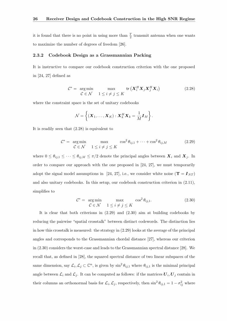
2.3.2 Codebook Design as a Grassmannian Packing
It is instructive to compare our codebook construction criterion with the one proposed
in [24, 27] defined as
C∗ = arg minC ∈ N
max1 ≤ i 6= j ≤ K
tr(XH
i XjXHj Xi
)(2.28)
where the constraint space is the set of unitary codebooks
N =
(X1, . . . , XK) : XH
k Xk =1
MIM
.
It is readily seen that (2.28) is equivalent to
C∗ = arg minC ∈ N
max1 ≤ i 6= j ≤ K
cos2 θij,1 + · · ·+ cos2 θij,M (2.29)
where 0 ≤ θij,1 ≤ · · · ≤ θij,M ≤ π/2 denote the principal angles between X i and Xj . In
order to compare our approach with the one proposed in [24, 27], we must temporarily
adopt the signal model assumptions in [24, 27], i.e., we consider white noise (Υ = INT )
and also unitary codebooks. In this setup, our codebook construction criterion in (2.11),
simplifies to
C∗ = arg minC ∈ N
max1 ≤ i 6= j ≤ K
cos2 θij,1. (2.30)
It is clear that both criterions in (2.29) and (2.30) aim at building codebooks by
reducing the pairwise “spatial crosstalk” between distinct codewords. The distinction lies
in how this crosstalk is measured: the strategy in (2.29) looks at the average of the principal
angles and corresponds to the Grassmannian chordal distance [27], whereas our criterion
in (2.30) considers the worst-case and leads to the Grassmannian spectral distance [28]. We
recall that, as defined in [28], the squared spectral distance of two linear subspaces of the
same dimension, say Li,Lj ⊂ Cn, is given by sin2 θij,1 where θij,1 is the minimal principal
angle between Li and Lj . It can be computed as follows: if the matrices U i, U j contain in
their columns an orthonormal basis for Li,Lj , respectively, then sin2 θij,1 = 1− σ2ij where
2.3 Considerations About the New Codebook Merit Function 27
σij is the maximal singular value of UHi U j . Given this definition, it follows that sin2 θij,1
corresponds to the squared spectral distance between the codewords X i and Xj (more
precisely, between their respective range spaces). Please refer to [28] and [54] for more
details on packing problems in Grassmannian space. The reader is referred to [55] for
a more in depth discussion on the geometry of complex Grassmann manifolds regarding
distance, cut and conjugate locus, etc.
We note that, for this particular scenario, the criterion presented in (2.28) is easier
to deal with mathematically. Also, from (2.30) we see that, for M = 1, the problem of
finding good codes coincides with the very well known packing problem in the complex
projective space [28].
2.3.3 Maximal Diversity Analysis
The method proposed in (2.10) and (2.11) is a numerical method as, for example, the ones
of [27] and [29]. A very interesting theoretical point is whether the method guarantees the
maximal diversity. Remark that the aforementioned references were not able to guarantee
the maximal diversity to their codes. In the following, we provide an analysis of this topic.
We will assume uncorrelated Rayleigh fading channel, i.e., hijiid∼ CN
(0, σ2
). In this
case,
SNR =E[∥∥XkH
H∥∥2]
E[‖E‖2
] =Nσ2
tr(Υ).
For a two point constellation (K = 2), the probability of error is given by
Pe = 0.5 E[PX1→X2+ PX2→X1
]
= 0.5 E
[Q(
1√2
√gH L12g
)+Q
(1√2
√gH L21g
)](2.31)
where the expectations are over the channel g = vec(HH
). Note that g ∼ CN
(0, σ2IMN
).
28 Receiver Design and Codebook Construction in the High SNR Regime
We proceed as
Pe ≤ 0.5 E
[exp−1
4gH L12g
]+ 0.5 E
[exp−1
4gH L21g
](2.32)
= 0.5
(1
det(IMN + σ2
4 L12)+
1
det(IMN + σ2
4 L21)
)(2.33)
≤ 0.5
1(1 + σ2
4 λmin(L12))MN
+1
(1 + σ2
4 λmin(L21))MN
(2.34)
≤ SNR−MN
(4N
tr(Υ)f12
)MN
(2.35)
where f12 = minλmin(L12), λmin(L21). The inequality (2.32) is the Chernoff upper bound
Q(x) ≤ e−x2/2
applied to (2.31), see section 2.1.5 in [56]. The equation (2.33) is due to the following
formula: if z∼CN (µ, K) and L = LH 0, then
E[exp−zHLz] =exp−µHL(I + KL)−1µ
det(I + KL),
see equation (5.59), page 194 in [21]. Inequality (2.34) is obtained by using the fact that,
for an n× n Hermitian matrix L = LH 0, we have
det (In + L) ≥ (1 + λmin (L))n .
Now, if the range space of the codeworks X1 and X2 do not share a line then both
L12 and L21 are positive-definite, i.e.,
λmin (L12) > 0 λmin (L21) > 0.
Thus, at high SNR (channel power σ2 → +∞), we have
1 +σ2
4λmin (Lij) ≈
σ2
4λmin (Lij).
Note the importance of having λmin (Lij) > 0 in the above approximation. From this, it
is straightforward to attain (2.35).

2.4 Codebook Construction 29
This line of reasoning is readily extended to the UB:
Pe ≤ UB =1
K
K∑
i=1
K∑
j = 1j 6= i
PXi→Xj
≤ 1
K
K∑
i=1
K∑
j = 1j 6= i
SNR−MN
(4N
tr(Υ)λmin (Lij)
)MN
≤ (K − 1)SNR−MN
(4N
tr(Υ)f
)MN
where
f = min λmin (Lij : i 6= j) .
What all this analysis shows is that, as long as we have a codebook C = X1, . . . , XK
which makes the matrices Lij (i 6= j) definite-positive (for which T ≥ 2M is necessary,
see subsection 2.3.1), then full-diversity is secured. But, what our design method tries to
achieve is exactly the maximization of
min λmin (Lij : i 6= j) ,
see equations (2.10) and (2.11). Although we are not able to furnish a theoretical proof
that our algorithm actually guarantees full diversity for any combination of T , K, M , N
and Υ, in all simulations presented afterwards the condition f > 0 is fulfilled.
2.4 Codebook Construction
We propose a two-phase methodology to tackle the optimization problem in (2.11). In
phase one, we start by solving a convex semi-definite programming (SDP) relaxation to
obtain a rough estimate of the optimal codebook. Phase two refines it through a geodesic
descent optimization algorithm (GDA) which efficiently exploits the Riemannian geometry
of the constraints. Suppose a codebook of size K is desired. In table 2.1, page 30 we give
the strategy that has shown to be effective.
The algorithm presented in table 2.1 is of the greedy type. We now explain Steps (3)
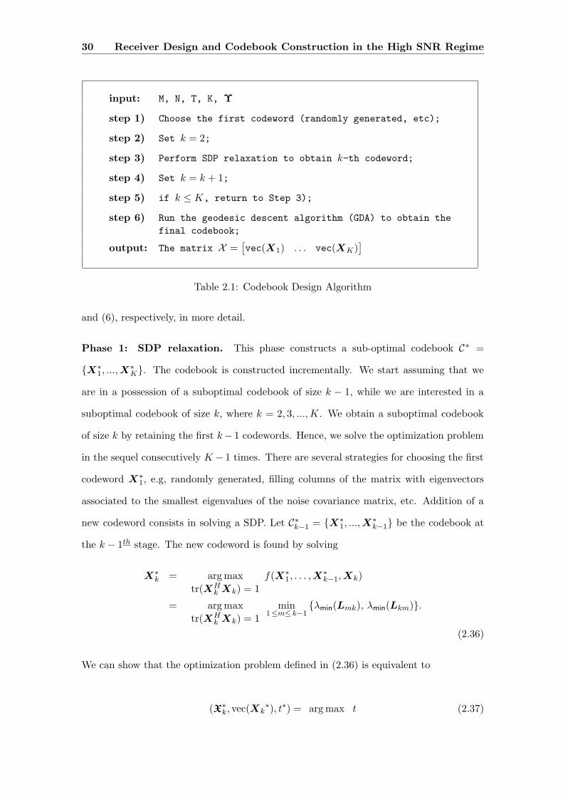
30 Receiver Design and Codebook Construction in the High SNR Regime
input: M, N, T, K, Υ
step 1) Choose the first codeword (randomly generated, etc);
step 2) Set k = 2;
step 3) Perform SDP relaxation to obtain k-th codeword;
step 4) Set k = k + 1;
step 5) if k ≤ K, return to Step 3);
step 6) Run the geodesic descent algorithm (GDA) to obtain the
final codebook;
output: The matrix X =[vec(X1) . . . vec(XK)
]
Table 2.1: Codebook Design Algorithm
and (6), respectively, in more detail.
Phase 1: SDP relaxation. This phase constructs a sub-optimal codebook C∗ =
X∗1, ..., X
∗K. The codebook is constructed incrementally. We start assuming that we
are in a possession of a suboptimal codebook of size k − 1, while we are interested in a
suboptimal codebook of size k, where k = 2, 3, ..., K. We obtain a suboptimal codebook
of size k by retaining the first k− 1 codewords. Hence, we solve the optimization problem
in the sequel consecutively K − 1 times. There are several strategies for choosing the first
codeword X∗1, e.g, randomly generated, filling columns of the matrix with eigenvectors
associated to the smallest eigenvalues of the noise covariance matrix, etc. Addition of a
new codeword consists in solving a SDP. Let C∗k−1 = X∗1, ..., X
∗k−1 be the codebook at
the k − 1th stage. The new codeword is found by solving
X∗k = arg max
tr(XHk Xk) = 1
f(X∗1, . . . , X
∗k−1, Xk)
= arg max
tr(XHk Xk) = 1
min1≤m≤ k−1
λmin(Lmk), λmin(Lkm).
(2.36)
We can show that the optimization problem defined in (2.36) is equivalent to
(X∗k, vec(Xk
∗), t∗) = arg max t (2.37)

2.4 Codebook Construction 31
with the following constraints
LMIAm(Xk, vec(Xk), t) 0, m = 1, ..., k − 1
LMIBm(Xk, vec(Xk), t) 0, m = 1, ..., k − 1
tr(Xk) = 1, Xk = vec(Xk)vecH(Xk) (2.38)
where the abbreviations LMIAm(Xk, vec(Xk), t) and LMIBm
(Xk, vec(Xk), t) denote lin-
ear (actually, affine) matrix inequalities in the variables Xk, vec(Xk), and t of type A and
B, respectively, for m = 1, ..., k − 1. The proof and the meaning of the LMI’s of type A
and B are given in Appendix B.
Due to the rank condition in (2.38) (note that the equations Xk = vec(Xk)vecH(Xk)
and tr(Xk) = 1 imply that rank (Xk) = 1), the design of the codewords, once again, trans-
lates into a difficult nonlinear optimization problem. However, relaxing this restriction
as
Xk vec(Xk)vecH(Xk) (2.39)
and rewriting (2.39) as
[Xk vec(Xk)
vecH(Xk) 1
] 0
the optimization problem in (2.37) becomes
(X∗k, vec(Xk
∗), t∗) = arg max t (2.40)
with the constraints
LMIAm(Xk, vec(Xk), t) 0, m = 1, ..., k − 1
LMIBm(Xk, vec(Xk), t) 0, m = 1, ..., k − 1
tr(Xk) = 1,
[Xk vec(Xk)
vecH(Xk) 1
] 0.
The rank 1 relaxation is usually known as the Shor relaxation [57]. The optimization
problem in (2.40) is a convex one in the variables Xk, vec(Xk) and t. Remark that for
K = 256, M = 2, N = 2, T = 8 and in the last passage through the loop, i.e., for k = K,

32 Receiver Design and Codebook Construction in the High SNR Regime
the output variable Xk is of dimension 16 × 16 (does not depend on N and K) and the
number of linear matrix inequality constraints that needs to be defined is of order K.
To solve the optimization problem in (2.40) we used the Self-Dual-Minimization package
SeDuMi 1.1 [58]. Once the problem defined in (2.40) is solved we need to extract the kth
codeword from the output variable Xk. Toward this end, we adopt a technique similar
to [62]. The technique consists in generating independent realizations of random vectors
that follow a Gaussian distribution with zero mean and covariance matrix Xk, i.e., zliid∼
CN (0, Xk) , for l = 1, 2, ..., L, where L is a parameter to be chosen (in all simulations
herein presented we assumed L = 1000). After forcing norm 1, i.e., vl = zl/||zl|| for
l = 1, 2, ..., L, we choose the k − th codeword, X∗k = ivec(vl∗) where
l∗ = arg maxl = 1, 2, ..., L
f(X∗1, X
∗2, ..., X
∗k−1, ivec(vl)). (2.41)
The operation “ivec” operates as an inverse of “vec” (reshapes the TM -dimensional vector
into a T ×M matrix). Note that X∗k is a valid codeword because tr(X∗H
k X∗k) = 1. We
are clearly dealing with a suboptimal solution for a codebook.
Phase 2: Geodesic Descent Algorithm. Problem (2.11) requires the optimization of
a non-smooth function over the smooth manifold M (Cartesian product of K spheres).
After phase 1, i.e., having solved the optimization problem (2.40) consecutively K − 1
times, for k = 2,3,..,K, we are now in possession of a suboptimal codebook of size K.
To refine it we resort to an iterative algorithm, which we call GDA (geodesic descent
algorithm). In table 2.2 we explain the GDA in more detail.
Let Ck be the kth iterate (the initialization C0 is furnished by phase 1). Note that the
power constraint tr(XHi Xi) = 1, for i = 1, 2, ..., K, can be equivalently written as
xTi xi = 1,
where
xi =
[<vec(X i)= vec(X i)
]∈ R
2TM ,
and <· and =· denote the real and imaginary part of a complex quantity, respectively.
In step 3 each xi, i = 1, ..., K is used to construct the vector x. In step 4 we identify the
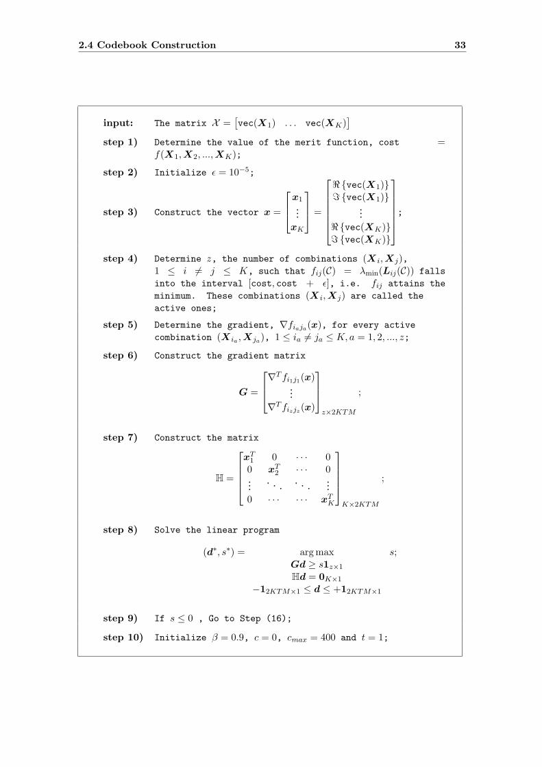
2.4 Codebook Construction 33
input: The matrix X =[vec(X1) . . . vec(XK)
]
step 1) Determine the value of the merit function, cost =f(X1, X2, ..., XK);
step 2) Initialize ε = 10−5;
step 3) Construct the vector x =
x1...
xK
=
<vec(X1)= vec(X1)
...
<vec(XK)= vec(XK)
;
step 4) Determine z, the number of combinations (X i, Xj),1 ≤ i 6= j ≤ K, such that fij(C) = λmin(Lij(C)) falls
into the interval [cost, cost + ε], i.e. fij attains the
minimum. These combinations (X i, Xj) are called the
active ones;
step 5) Determine the gradient, ∇fiaja(x), for every active
combination (X ia , Xja), 1 ≤ ia 6= ja ≤ K, a = 1, 2, ..., z;
step 6) Construct the gradient matrix
G =
∇T fi1j1(x)
...
∇T fizjz(x)
z×2KTM
;
step 7) Construct the matrix
H =
xT1 0 · · · 00 xT
2 · · · 0...
......
...
0 · · · · · · xTK
K×2KTM
;
step 8) Solve the linear program
(d∗, s∗) = arg maxGd ≥ s1z×1
Hd = 0K×1
−12KTM×1 ≤ d ≤ +12KTM×1
s;
step 9) If s ≤ 0 , Go to Step (16);
step 10) Initialize β = 0.9, c = 0, cmax = 400 and t = 1;
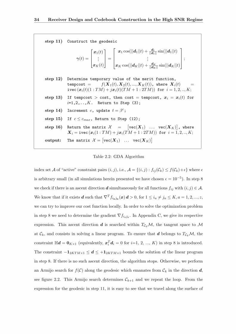
34 Receiver Design and Codebook Construction in the High SNR Regime
step 11) Construct the geodesic
γ(t) =
x1(t)...
xK(t)
=
x1 cos(||d1||t) + d1
||d1|| sin(||d1||t)...
xK cos(||dK ||t) + dK
||dK || sin(||dK ||t)
;
step 12) Determine temporary value of the merit function,
tempcost = f(X1(t), X2(t), ..., XK(t)), where X i(t) =ivec (xi(t)(1 : TM) + jxi(t)(TM + 1 : 2TM)) for i = 1, 2, .., K;
step 13) If tempcost > cost, then cost = tempcost, xi = xi(t) for
i=1,2,..,K. Return to Step (3);
step 14) Increment c, update t = βc;
step 15) If c ≤ cmax, Return to Step (12);
step 16) Return the matrix X =[vec(X1) . . . vec(XK)
], where
Xi = ivec (xi(1 : TM) + jxi(TM + 1 : 2TM)) for i = 1, 2, .., K;
output: The matrix X =[vec(X1) . . . vec(XK)
]
Table 2.2: GDA Algorithm
index set A of “active” constraint pairs (i, j), i.e., A = (i, j) : fij(Ck) ≤ f(Ck)+ε where ε
is arbitrary small (in all simulations herein presented we have chosen ε = 10−5). In step 8
we check if there is an ascent direction d simultaneously for all functions fij with (i, j) ∈ A.
We know that if it exists d such that ∇T fiaja(x) d > 0, for 1 ≤ ia 6= ja ≤ K, a = 1, 2, ..., z,
we can try to improve our cost function locally. In order to solve the optimization problem
in step 8 we need to determine the gradient ∇fiaja . In Appendix C, we give its respective
expression. This ascent direction d is searched within TCkM, the tangent space to M
at Ck, and consists in solving a linear program. To ensure that d belongs to TCkM, the
constraint Hd = 0K×1 (equivalently, xTi di = 0 for i=1, 2, ..., K) in step 8 is introduced.
The constraint −12KTM×1 ≤ d ≤ +12KTM×1 bounds the solution of the linear program
in step 8. If there is no such ascent direction, the algorithm stops. Otherwise, we perform
an Armijo search for f(C) along the geodesic which emanates from Ck in the direction d,
see figure 2.2. This Armijo search determines Ck+1 and we repeat the loop. From the
expression for the geodesic in step 11, it is easy to see that we travel along the surface of
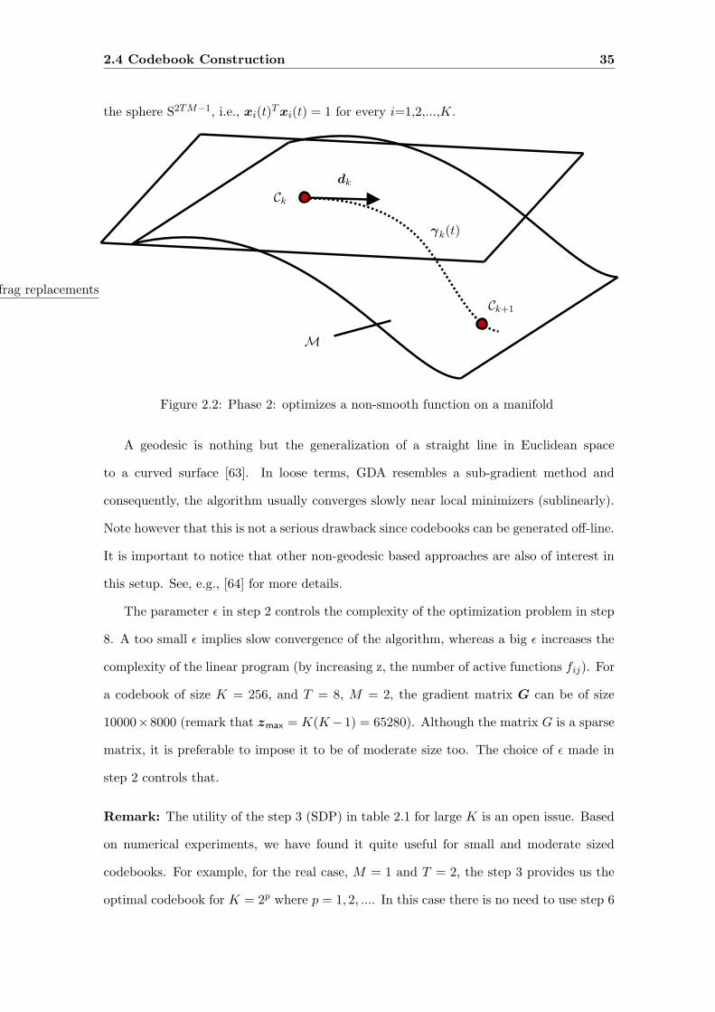
2.4 Codebook Construction 35
the sphere S2TM−1, i.e., xi(t)T xi(t) = 1 for every i=1,2,...,K.
PSfrag replacements
Ck
γk(t)
Ck+1
dk
M
Figure 2.2: Phase 2: optimizes a non-smooth function on a manifold
A geodesic is nothing but the generalization of a straight line in Euclidean space
to a curved surface [63]. In loose terms, GDA resembles a sub-gradient method and
consequently, the algorithm usually converges slowly near local minimizers (sublinearly).
Note however that this is not a serious drawback since codebooks can be generated off-line.
It is important to notice that other non-geodesic based approaches are also of interest in
this setup. See, e.g., [64] for more details.
The parameter ε in step 2 controls the complexity of the optimization problem in step
8. A too small ε implies slow convergence of the algorithm, whereas a big ε increases the
complexity of the linear program (by increasing z, the number of active functions fij). For
a codebook of size K = 256, and T = 8, M = 2, the gradient matrix G can be of size
10000×8000 (remark that zmax = K(K−1) = 65280). Although the matrix G is a sparse
matrix, it is preferable to impose it to be of moderate size too. The choice of ε made in
step 2 controls that.
Remark: The utility of the step 3 (SDP) in table 2.1 for large K is an open issue. Based
on numerical experiments, we have found it quite useful for small and moderate sized
codebooks. For example, for the real case, M = 1 and T = 2, the step 3 provides us the
optimal codebook for K = 2p where p = 1, 2, .... In this case there is no need to use step 6
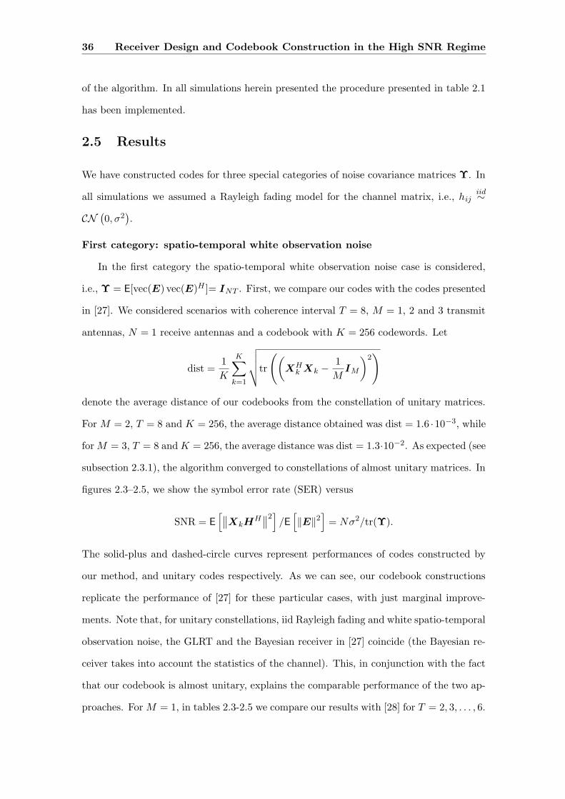
36 Receiver Design and Codebook Construction in the High SNR Regime
of the algorithm. In all simulations herein presented the procedure presented in table 2.1
has been implemented.
2.5 Results
We have constructed codes for three special categories of noise covariance matrices Υ. In
all simulations we assumed a Rayleigh fading model for the channel matrix, i.e., hijiid∼
CN(0, σ2
).
First category: spatio-temporal white observation noise
In the first category the spatio-temporal white observation noise case is considered,
i.e., Υ = E[vec(E) vec(E)H ]= INT . First, we compare our codes with the codes presented
in [27]. We considered scenarios with coherence interval T = 8, M = 1, 2 and 3 transmit
antennas, N = 1 receive antennas and a codebook with K = 256 codewords. Let
dist =1
K
K∑
k=1
√√√√tr
((XH
k Xk −1
MIM
)2)
denote the average distance of our codebooks from the constellation of unitary matrices.
For M = 2, T = 8 and K = 256, the average distance obtained was dist = 1.6 ·10−3, while
for M = 3, T = 8 and K = 256, the average distance was dist = 1.3·10−2. As expected (see
subsection 2.3.1), the algorithm converged to constellations of almost unitary matrices. In
figures 2.3–2.5, we show the symbol error rate (SER) versus
SNR = E[∥∥XkH
H∥∥2]/E[‖E‖2
]= Nσ2/tr(Υ).
The solid-plus and dashed-circle curves represent performances of codes constructed by
our method, and unitary codes respectively. As we can see, our codebook constructions
replicate the performance of [27] for these particular cases, with just marginal improve-
ments. Note that, for unitary constellations, iid Rayleigh fading and white spatio-temporal
observation noise, the GLRT and the Bayesian receiver in [27] coincide (the Bayesian re-
ceiver takes into account the statistics of the channel). This, in conjunction with the fact
that our codebook is almost unitary, explains the comparable performance of the two ap-
proaches. For M = 1, in tables 2.3-2.5 we compare our results with [28] for T = 2, 3, . . . , 6.
2.5 Results 37
We manage to improve the best known results and in some cases actually provide optimal
packings, i.e., equiangular tight frames (ETFs), which attain the Rankin upper bound
(equivalently, the Welch lower bound [65]). For the sake of completeness a comparison
with unitary codes found in [32] is also performed. Figure 2.6 shows the result of the
experiment for T = 4, M = 2, N = 2 and K = 256. We observe that our codes show
almost no improvement over the constructions presented in [32].
0 5 10 15 20 2510
−5
10−4
10−3
10−2
10−1
100
SNR (dB)
SE
R
Figure 2.3: Category 1 - spatio-temporally white observation noise: T = 8, M = 3, N = 1,K = 256, Υ = INT . Plus-solid curve:our codes; circle-dashed curve:unitary codes.
Second category: spatially white-temporally colored observation noise
The second category corresponds to spatially white-temporally colored observation
noise, i.e., Υ = IN ⊗ Σ(ρ) where the vector ρ : T × 1 is the first column of an Hermitian
Toeplitz matrix Σ(ρ). To the best of our knowledge, we are not aware of any work
that treats the problem of codebook constructions in the presence of spatially white-
temporally colored observation noise. Hence, we compare our codes designed (adapted) to
this specific scenario with unitary codes [27]. The goal here is to demonstrate the increase
of performance obtained by matching the codebook construction to the noise statistics.
In figures 2.7–2.9 the solid curves represent the performance of codes constructed by our
method, while the dashed curves represent the performance of unitary codes. In either

38 Receiver Design and Codebook Construction in the High SNR Regime
PACKING RADII (DEGREES)
T K MB JAT Rankin
2 3 60 60 60
2 4 54.74 54.74 54.74
2 5 45.00 45.00 52.24
2 6 45.00 45.00 50.77
2 7 38.93 38.93 49.80
2 8 37.43 37.41 49.11
2 9 35.26 − 48.59
2 10 33.07 − 48.19
2 11 31.72 − 47.87
2 12 31.72 − 47.61
2 13 28.24 − 47.39
2 14 27.83 − 47.21
2 15 26.67 − 47.05
2 16 25.97 − 46.91
3 4 70.53 70.53 70.53
3 5 64.26 64.00 65.91
3 6 63.43 63.43 63.43
3 7 61.87 61.87 61.87
3 8 60.00 60.00 60.79
3 9 60.00 60.00 60.00
3 10 54.74 54.73 59.39
3 11 54.74 54.73 58.91
3 12 54.74 54.73 58.52
3 13 51.38 51.32 58.19
3 14 50.36 50.13 57.92
3 15 49.80 49.53 57.69
3 16 49.61 49.53 57.49
3 17 49.13 49.10 57.31
3 18 48.12 48.07 57.16
Table 2.3: PACKING IN COMPLEX PROJECTIVE SPACE: We compare our best con-figurations (MB) of K points in P
T−1(C) against the Tropp codes (JAT) and Rankinbound [28]. The packing radius of an ensemble is measured as the acute angle betweenthe closest pair of lines. Minus sign symbol (-) means that no packing is available forspecific pair (T, K).
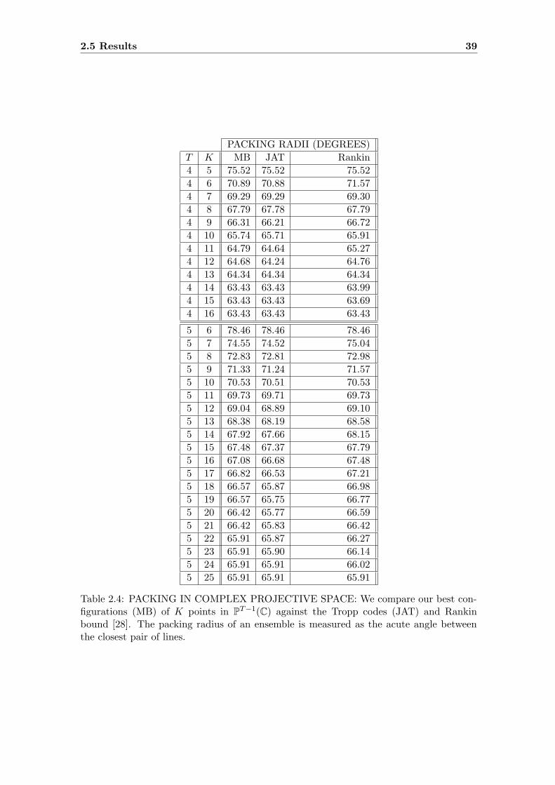
2.5 Results 39
PACKING RADII (DEGREES)
T K MB JAT Rankin
4 5 75.52 75.52 75.52
4 6 70.89 70.88 71.57
4 7 69.29 69.29 69.30
4 8 67.79 67.78 67.79
4 9 66.31 66.21 66.72
4 10 65.74 65.71 65.91
4 11 64.79 64.64 65.27
4 12 64.68 64.24 64.76
4 13 64.34 64.34 64.34
4 14 63.43 63.43 63.99
4 15 63.43 63.43 63.69
4 16 63.43 63.43 63.43
5 6 78.46 78.46 78.46
5 7 74.55 74.52 75.04
5 8 72.83 72.81 72.98
5 9 71.33 71.24 71.57
5 10 70.53 70.51 70.53
5 11 69.73 69.71 69.73
5 12 69.04 68.89 69.10
5 13 68.38 68.19 68.58
5 14 67.92 67.66 68.15
5 15 67.48 67.37 67.79
5 16 67.08 66.68 67.48
5 17 66.82 66.53 67.21
5 18 66.57 65.87 66.98
5 19 66.57 65.75 66.77
5 20 66.42 65.77 66.59
5 21 66.42 65.83 66.42
5 22 65.91 65.87 66.27
5 23 65.91 65.90 66.14
5 24 65.91 65.91 66.02
5 25 65.91 65.91 65.91
Table 2.4: PACKING IN COMPLEX PROJECTIVE SPACE: We compare our best con-figurations (MB) of K points in P
T−1(C) against the Tropp codes (JAT) and Rankinbound [28]. The packing radius of an ensemble is measured as the acute angle betweenthe closest pair of lines.

40 Receiver Design and Codebook Construction in the High SNR Regime
0 5 10 15 20 25 3010
−5
10−4
10−3
10−2
10−1
100
SNR (dB)
SE
R
Figure 2.4: Category 1 - spatio-temporally white observation noise: T = 8, M = 2, N = 1,K = 256, Υ = INT . Plus-solid curve: our codes; circle-dashed curve: unitary codes.
case, the plus sign indicates that the GLRT receiver is implemented. The square sign
indicates that the Bayesian receiver is implemented. Figure 2.7 plots the result of the
experiment for T = 8, M = 2, N = 1, K = 67 and ρ = [ 1; 0.85; 0.6; 0.35; 0.1;
zeros(3,1) ]. It can be seen that for SER = 10−3, our codes demonstrate a gain of 3 dB
when compared with the unitary codes. Figure 2.8 plots the result of the experiment for
T = 8, M = 2, N = 1, K = 256 and ρ =[ 1; 0.8; 0.5; 0.15; zeros(4,1) ]. For SER = 10−3
our codes demonstrate gain of 2 dB when compared with unitary codes. Figure 2.9 plots
the result of the experiment for T = 8, M = 2, N = 1, K = 32 and ρ =[ 1; 0.8; 0.5;
0.15; zeros(4,1) ]. For SER = 10−3, our codes demonstrate gain of 3 dB when compared
with the unitary codes. In figures 2.7- 2.9, the dotted curve represents the performance of
the codes obtained by the heuristic codebook C defined in (2.12), and dash-dotted curve
represents the performance of the codes obtained by the heuristic codebook C defined
in (2.13). As can be seen, this leads to a degradation of performance, even with respect
to plain unitary codebooks (dashed curves).
We have also performed a comparison with unitary codes found in [32]. Figure 2.10
shows the result of the experiment for T = 4, M = 2, N = 2, K = 256 and ρ =[ 1;

2.5 Results 41
0 5 10 15 20 25 3010
−3
10−2
10−1
100
SNR (dB)
SE
R
Figure 2.5: Category 1 - spatio-temporally white observation noise: T = 8, M = 1, N = 1,K = 256, Υ = INT . Plus-solid curve: our codes; circle-dashed curve: unitary codes.
0.8 ; 0.6; 0.1 ]. We see that for SER = 10−3 our codes demonstrate a gain of 2 dB when
compared with the unitary codes.
Third category: E = s αT + Etemp
In the third category, we considered the case where the noise matrix is of the form E =
s αT + Etemp. This models an interfering source s (with known covariance matrix Υs)
where the complex vector α is the known channel attenuation between each receive antenna
and the interfering source. The matrix Etemp has a noise covariance matrix belonging
to the second category. Thus, the noise covariance matrix is given by Υ = ααH ⊗Υs +
IN ⊗ Σ(ρ). As for the second category, we compare our codes adapted to this particular
scenario with unitary codes. In figures 2.11–2.12 the solid curves represent performance
of codes constructed by our method, while the dashed curves represent performance of
unitary codes [27]. Figure 2.11 plots the result of the experiment for T = 8, M = 2,
N = 2, K = 32, s =[1; 0.7; 0.4; 0.15; zeros(4,1)], ρ = [1; 0.8; 0.5; 0.15; zeros(4,1)] and
α = [-1.146 + 1.189i;1.191- 0.038i]. For SER = 10−3, once again our codes demonstrate
a gain of more than 2 dB gain when compared with the unitary codes. Figure 2.12 plots
the result of the experiment for T = 8, M = 2, N = 2, K = 67, ρ =[1; 0.7; 0.4; 0.15;
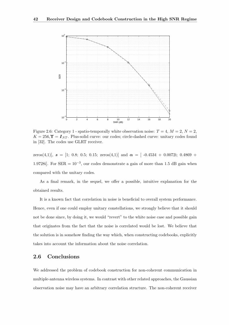
42 Receiver Design and Codebook Construction in the High SNR Regime
0 2 4 6 8 10 12 14 16 18 2010
−3
10−2
10−1
100
SNR (dB)
SE
R
Figure 2.6: Category 1 - spatio-temporally white observation noise: T = 4, M = 2, N = 2,K = 256,Υ = INT . Plus-solid curve: our codes; circle-dashed curve: unitary codes foundin [32]. The codes use GLRT receiver.
zeros(4,1)], s = [1; 0.8; 0.5; 0.15; zeros(4,1)] and α = [ -0.4534 + 0.0072i; 0.4869 +
1.9728i]. For SER = 10−3, our codes demonstrate a gain of more than 1.5 dB gain when
compared with the unitary codes.
As a final remark, in the sequel, we offer a possible, intuitive explanation for the
obtained results.
It is a known fact that correlation in noise is beneficial to overall system performance.
Hence, even if one could employ unitary constellations, we strongly believe that it should
not be done since, by doing it, we would “revert” to the white noise case and possible gain
that originates from the fact that the noise is correlated would be lost. We believe that
the solution is in somehow finding the way which, when constructing codebooks, explicitly
takes into account the information about the noise correlation.
2.6 Conclusions
We addressed the problem of codebook construction for non-coherent communication in
multiple-antenna wireless systems. In contrast with other related approaches, the Gaussian
observation noise may have an arbitrary correlation structure. The non-coherent receiver

2.6 Conclusions 43
PACKING RADII (DEGREES)
T K MB Rankin
6 7 80.41 80.41
6 8 77.06 77.40
6 9 75.52 75.52
6 10 74.20 74.21
6 11 73.22 73.22
6 12 72.45 72.45
6 13 71.82 71.83
6 14 71.31 71.32
6 15 70.87 70.89
6 16 70.53 70.53
6 17 70.10 70.21
6 18 69.73 69.94
6 19 69.40 69.70
Table 2.5: PACKING IN COMPLEX PROJECTIVE SPACE: We compare our best con-figurations (MB) of K points in P
T−1(C) against Rankin bound [28]. The packing radiusof an ensemble is measured as the acute angle between the closest pair of lines.
operates according to the GLRT principle. A methodology for designing space-time code-
books for this non-coherent setup, taking the probability of error of the detector in the
high SNR regime as the code design criterion, is proposed. We have presented a two-phase
greedy approach to solve the resulting high-dimensional, nonlinear and non-smooth opti-
mization problem. The first phase solves a convex SDP relaxation to obtain a suboptimal
codebook. The second phase refines it through a geodesic descent optimization algorithm
which efficiently exploits the Riemannian geometry of the constraints. Computer simu-
lations show that our codebooks are marginally better than state-of-art known solutions
for the special case of spatio-temporal white Gaussian observation noise but significantly
outperform them in the correlated noise environments. This shows the relevance of the
codebook construction tool proposed herein.

44 Receiver Design and Codebook Construction in the High SNR Regime
0 2 4 6 8 10 1210
−4
10−3
10−2
10−1
100
SNR (dB)
SE
R
Figure 2.7: Category 2 - spatially white - temporally colored: T = 8, M = 2, N = 1,K = 67, ρ =[ 1; 0.85; 0.6; 0.35; 0.1; zeros(3,1) ]. Solid curves: our codes; dashed curves:unitary codes; dotted curve: codes obtained by the heuristic (2.12); dash-dotted curve:codes obtained by the heuristic (2.13); plus signed curves: GLRT receiver; square signedcurves: Bayesian receiver.
0 2 4 6 8 10 12 14 16 1810
−4
10−3
10−2
10−1
100
SNR
SE
R
Figure 2.8: Category 2 - spatially white - temporally colored: T = 8, M = 2, N = 1,K = 256, ρ =[ 1; 0.8; 0.5; 0.15; zeros(4,1) ]. Solid curves: our codes; dashed curves:unitary codes; dotted curve: codes obtained by the heuristic (2.12); dash-dotted curve:codes obtained by the heuristic (2.13); plus signed curves: GLRT receiver; square signedcurves: Bayesian receiver.
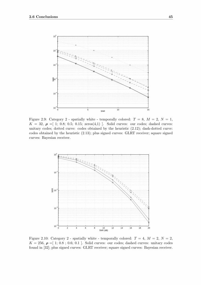
2.6 Conclusions 45
0 5 10 1510
−5
10−4
10−3
10−2
10−1
100
SNR
SE
R
Figure 2.9: Category 2 - spatially white - temporally colored: T = 8, M = 2, N = 1,K = 32, ρ =[ 1; 0.8; 0.5; 0.15; zeros(4,1) ]. Solid curves: our codes; dashed curves:unitary codes; dotted curve: codes obtained by the heuristic (2.12); dash-dotted curve:codes obtained by the heuristic (2.13); plus signed curves: GLRT receiver; square signedcurves: Bayesian receiver.
0 2 4 6 8 10 12 14 16 18 2010
−4
10−3
10−2
10−1
100
SNR (dB)
SE
R
Figure 2.10: Category 2 - spatially white - temporally colored: T = 4, M = 2, N = 2,K = 256, ρ =[ 1; 0.8 ; 0.6; 0.1 ]. Solid curves: our codes; dashed curves: unitary codesfound in [32]; plus signed curves: GLRT receiver; square signed curves: Bayesian receiver.
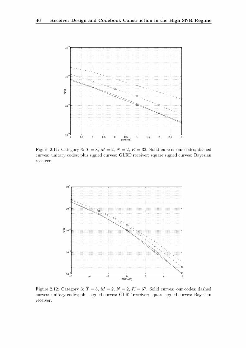
46 Receiver Design and Codebook Construction in the High SNR Regime
−2 −1.5 −1 −0.5 0 0.5 1 1.5 2 2.5 310
−4
10−3
10−2
10−1
SNR (dB)
SE
R
Figure 2.11: Category 3: T = 8, M = 2, N = 2, K = 32. Solid curves: our codes; dashedcurves: unitary codes; plus signed curves: GLRT receiver; square signed curves: Bayesianreceiver.
−6 −4 −2 0 2 4 610
−4
10−3
10−2
10−1
100
SNR (dB)
SE
R
Figure 2.12: Category 3: T = 8, M = 2, N = 2, K = 67. Solid curves: our codes; dashedcurves: unitary codes; plus signed curves: GLRT receiver; square signed curves: Bayesianreceiver.
Chapter 3
Capacity and Error Probability
Analysis of Non-Coherent MIMO
Systems in the Low SNR Regime
3.1 Chapter Summary
The chapter is organized as follows. In section 3.2, the spatially correlated non-coherent
MIMO block Rayleigh fading channel is analyzed. The impact of channel and noise cor-
relation on the mutual information is obtained for the on-off and Gaussian signaling. In
section 3.3, contrary to most approaches for the low SNR regime, a low SNR analysis of the
PEP for the GLRT receiver is introduced, and a codebook design criterion which takes
into account the information about noise correlation is obtained. New space-time con-
stellations for some particular wireless scenarios are constructed. Computer simulations
show that these new codebooks are also of interest for Bayesian receivers which decode
constellations with non-uniform priors. Section 3.4 contains the main conclusions of this
chapter.
3.2 Random Fading Channel: the Low SNR Mutual Infor-
mation Analysis
Data model and assumptions. We focus on a communication system comprising M
transmit and N receive antennas over a narrowband flat Rayleigh fading channel. We
assume a block fading channel model which is widely used in the MIMO literature [23,
45, 46, 66], with coherence interval T . In complex base band notation we have the system
47
48Capacity and Error Probability Analysis of Non-Coherent MIMO Systems in
the Low SNR Regime
model
Y = XHH + E, (3.1)
where X is the T ×M matrix of transmitted symbols, Y is the T ×N matrix of received
symbols, HH is the M ×N matrix of channel coefficients, and E is the T ×N matrix of
zero-mean additive observation noise. For for the sake of convenience, let H = HH . We
work under the following assumptions:
B1. (Channel matrix) The popular separable (Kronecker) spatial correlation model [38,
66, 67] is used, i.e., H =√
ρM K
1
2
t Hw
(KT
r
) 1
2 where Hw is a M × N matrix com-
prised of statistically independent CN (0, 1) entries and the coefficient ρ is the model
parameter proportional to the SNR. We assume that the matrix Hw remains fixed
for the coherence time T after which it changes to a new independent value. The
correlation coefficients between the M (N) transmit (receive) antennas are assem-
bled into an M ×M (N ×N) positive semidefinite Hermitian correlation matrix K t
(KTr ; the operator T is used for the sake of convenience). The matrix Hw is not
known at the receiver nor at the transmitter, but its distribution is, in addition to
Kt and Kr. This model is appropriate for the scenarios where only the objects sur-
rounding the transmitter and the receiver cause the correlation of the local antenna
elements, while they have no impact on the correlation at the other end of the link.
The model has been found to be satisfactory in certain scenarios [68, 69]. We would
also like to point out that there exist other spatial correlation models that take into
account coupling between transmit and receive sides, see [70] and references therein.
Although these models may characterize realistic channels more accurately for some
scenarios (in these cases, the Kronecker model leads to capacity underestimations),
in this work, we adopt the Kronecker model since we believe that it represents a
good compromise between analytical tractability and validity of the channel. For
a fair comparison of different correlation cases, we assume that tr(K t) = M and
tr(Kr) = N ;
B2. (Transmit power constraint) We impose the power constraint E[tr(XHX)] ≤

3.2 Random Fading Channel: the Low SNR Mutual Information Analysis 49
TM ;
B3. (Noise distribution) The noise covariance matrix Υ = E[vec(E) vec(E)H ] is
known at the transmitter and at the receiver. Also, without loss of generality
(w.l.o.g.), we assume tr(Υ) = NT .
Note that in B3, we again let the data model depart from the customary assumption
of spatio-temporal white Gaussian observation noise.
3.2.1 Mutual Information: On-Off Signaling
In [45], it has been demonstrated that the on-off signaling presented in [41], where the
single transmit antenna systems were considered, generalizes to the multi-antenna setting
and attains the ergodic channel capacity for the coherent case. Here, we show that this
is also the case for the correlated Rayleigh fading channel model with arbitrary noise
covariance matrix. Furthermore, we maximize the mutual information with respect to
(w.r.t.) the input signal Xon, Kt and Kr. Hence, we view both Kt and Kr as system
parameters which we can introduce and track. The on-off signaling is defined as: for any
ε > 1 and assuming ρ < 1,
X =
Xon ρ−
ε2 with probability (w.p.) ρε
0T×M w.p. 1− ρε
With an analysis similar to [45], presented in Appendix D, it can be shown that at suffi-
ciently low SNR the mutual information between Y and X up to first order in ρ is given
by
I(Y ; X) =ρ
Mtr(Υ−1
(Kr ⊗XonKtX
Hon
))+ o(ρ). (3.2)
Note that for the special case of spatio-temporal white observation noise and uncorrelated
Rayleigh fading channel case, i.e., Υ = ITN , Kt = IM and Kr = IN our result in (3.2)
recovers the finding in [45]. In that case, the maximal mutual information (per channel
use) is equal to
1
TI(Y ; X) = ρ N + o(ρ).

50Capacity and Error Probability Analysis of Non-Coherent MIMO Systems in
the Low SNR Regime
Now, we address the maximization of the mutual information w.r.t. Xon, Kt and Kr,
i.e.,
max
tr(XonXH
on
)≤ TM,
Kt ∈ PM , Kr ∈ PN
tr(Υ−1
(Kr ⊗XonKtX
Hon
))(3.3)
where
Pn = Q : n× n matrix such that Q 0 and tr (Q) = n. (3.4)
In Appendix E we show that the maximum in (3.3) is attained by
Xon =√
TM[x 0T×(M−1)
], Kr = N uuH ,
[Kt
]i,i
= Mδi1 (3.5)
where
(u, x) = arg maxu ∈ C
N , ||u|| = 1,x ∈ C
T , ||x|| = 1
(u⊗ x)H Υ−1 (u⊗ x) (3.6)
with δij = 1 for i = j and zero otherwise. The notation [M ]i,i represents the entry of the
matrix M on the position (i, i). Note that Kt is a diagonal matrix. The optimization
problem in (3.6) always admits a solution (maximization of a continuous function over a
compact set) but, in general, a closed form solution is not available. The exception is the
case when the noise covariance matrix Υ has a Kronecker structure, say Υ = Υ1 ⊗Υ2
for some N ×N matrix Υ1 and T × T matrix Υ2. In that situation, the optimal u (resp.
x) can be taken as any unit-norm eigenvector associated with the minimal eigenvalue of
Υ1 (resp. Υ2). For example, in the case of spatially white-temporally colored observation
noise, i.e., Υ = IN ⊗ Σ for some T × T positive definite matrix Σ, the vector x is the
unit-norm eigenvector associated with the minimal eigenvalue of Σ (in other words, we
transmit the codeword in the direction that is least affected by the noise). For the choice
in (3.5), the maximal mutual information (per channel use) is equal to
1
TI(Y ; X) = ρ N Mλ + o(ρ). (3.7)
where λ = (u⊗ x)H Υ−1 (u⊗ x).
Remarks. From (3.5) it is clear that both the transmit and receive antennas should be
made as correlated as possible, as both the optimal K t and Kr have rank one. Note

3.2 Random Fading Channel: the Low SNR Mutual Information Analysis 51
that in (3.7) the mutual information is proportional to the number of transmit antennas
M . This is in sharp contrast with the case of uncorrelated Rayleigh fading channel model
for which it has been shown that the maximal mutual information is independent of the
number of transmit antennas [45]. Also, since
tr(Υ−1
)=
NT∑
i=1
1/λi ≥NT∑
i=1
(2− λi) = NT,
where λi’s are the eigenvalues of Υ, we can w.l.o.g. assume that, e.g.,[Υ−1
]1,1≥ 1 (other-
wise tr(Υ−1
)< NT ). Then, by choosing u1 =
[1 01×(N−1)
]Tand x1 =
[1 01×(T−1)
]T
we have
λ ≥ (u1 ⊗ x1)H Υ−1 (u1 ⊗ x1) =
[Υ−1
]1,1≥ 1.
This result confirms the general principle that correlated noise is beneficial from the ca-
pacity point of view. See, e.g., pp. 100 in [18] for more details. In practice, by changing
the antenna separation one can control the eigenvalues of K t and Kr, but not their eigen-
vectors. See [46, 66, 71, 72], [18, section 6.3.3]. As a consequence, the result presented
herein has to be interpreted as the upper bound on the channel capacity. For guidelines
for optimizing antenna spacing in the case when there is little to no local scattering around
the base station and the mobile is assumed to be in a rich scattering environment, see [72].
For the physical conditions on the antenna spacing under which the Kronecker model is
appropriate, the reader is referred to pp. 98-100 in [71] for more details. Nevertheless,
the previous conclusion holds for the case when we can not manipulate the eigenvectors
of Kr (which are still available to the transmitter through a feedback link): in this case,
from (E.11) we obtain
1
TI(Y ; X) = ρ N Mλmax
(F i∗Υ
−1F H
i∗
)+ o(ρ)
where Υ, F i and i∗ are defined in (E.5), (E.5) and (E.8), respectively. It is clear that
λmax
(F i∗Υ
−1F H
i∗
)≥ 1 (otherwise tr(Υ−1) < NT ). Thus, correlated noise is beneficial
from the capacity point of view in this case too. A short exercise would show that the
first order term in (3.7) corresponds to that of the capacity when the channel is known
to the receiver and the noise covariance matrix Υ is arbitrary (when Υ = INT , then

52Capacity and Error Probability Analysis of Non-Coherent MIMO Systems in
the Low SNR Regime
λ = 1, from (3.7) we retrieve the result on pp. 94 in [18] where the coherent correlated
Rayleigh fading channel has been treated). With coherent reception, we know that the
mutual information is maximized if the input vec(X) is circularly symmetric, complex
Gaussian distribution, i.e., vec(X)∼CN (0, P coh) for some covariance matrix P coh with
tr(P coh) ≤ TM such that the power constraint in the assumption B2 is satisfied (note
that we may assume w.l.o.g. that vec(X) is zero-mean). In that case, the channel capacity
is given by
Ehw
[log2 det
(ITN +
ρ
MΥ− 1
2 (L⊗ IT ) P coh
(LH ⊗ IT
)Υ− 1
2
)](3.8)
where L = K1
2r HT
w
(KT
t
) 1
2 and hw = vec (Hw). It can be readily shown (by maximizing
the first-order expansion of (3.8) w.r.t. P coh, Kt and Kr) that the optimal covariance
matrix P coh is equal to
P coh = vec(Xon)vecH(Xon), (3.9)
with Xon, Kt and Kr defined as in (3.5).
3.2.2 Mutual Information: Gaussian Modulation
In this subsection, we compute the low SNR mutual information for the more realistic
and practical case of Gaussian modulation. Let x = vec(X) be a zero-mean random
variable with covariance matrix P that follows a circularly symmetric, complex Gaussian
distribution, i.e., x∼CN (0, P ). Clearly, in order to meet the power constraint in the
assumption B2, tr(P ) ≤ TM . Then, at sufficiently low SNR, the mutual information
between Y and X up to second order in ρ is given by
I(Y ; X) =ρ2
2M2tr(E[Z2]− (E[Z])2
)+ o(ρ2) (3.10)
=ρ2
2M2
M∑
i=1
M∑
j=1
N∑
k=1
N∑
z=1
λkλztr(ΥkzP ij)tr(ΥzkP ji) + o(ρ2), (3.11)
where
Z = Υ− 1
2
(Kr ⊗XKtX
H)Υ− 1
2 , P =
((KT
t
) 1
2 ⊗ IT
)P
((KT
t
) 1
2 ⊗ IT
),
P ij = EiPEHj , Υkz = F kΥ
−1F H
z

3.2 Random Fading Channel: the Low SNR Mutual Information Analysis 53
and λk’s, for k = 1, ..., N , are the eigenvalues of Kr. The matrices Υ and F k, for
k = 1, ..., N , are defined in (E.5), whereas the T ×TM matrix Ei, for i = 1, ..., M , is given
by
Ei = eTi ⊗ IT , (3.12)
where ei represents the i-th column of the identity matrix IM . The proof is given in
Appendix F. We now address the optimization problem
maxP 0, tr (P ) ≤ TM,Kt ∈ PM , Kr ∈ PN
M∑
i=1
M∑
j=1
N∑
k=1
N∑
z=1
λkλztr(ΥkzP ij)tr(ΥzkP ji). (3.13)
It can be shown that the maximum of (3.13) is attained by the following signaling scheme:
the optimal correlation matrices Kr and Kt are defined as in (3.5), and the optimal
covariance matrix P is given by
P = TMKP ⊗ xxH (3.14)
where the vectors u and x are, as before, solutions of the optimization problem (3.6).
The M ×M constant matrix KP has all the entries equal to zero except the entry (1,1)
which is one. The proof is given in Appendix G. In this case, the mutual information (per
channel use) is given by
1
TI(Y ; X) =
ρ2
2N2 T M2 λ2 + o(ρ2). (3.15)
where λ = (u⊗ x)H Υ−1 (u⊗ x).
Remarks. In [45] it has been proved that for the uncorrelated Rayleigh fading channel
only one transmit antenna should be employed. Here, we see from (3.15) that having more
transmit (M) and receive (N) antennas can actually enhance the channel performance in
terms of capacity significantly in the correlated setup. We see that the mutual information
is proportional to M 2N2, whereas in [45] the increase is only linear in the number of the
receive antennas. Hence, by making the antennas as correlated as possible the total
gain is M2N . Remark that although the mathematics for calculating P , Kt and Kr
are quite involved, our findings are not surprising since we see that the optimal values

54Capacity and Error Probability Analysis of Non-Coherent MIMO Systems in
the Low SNR Regime
correspond to those of the coherent correlated Rayleigh fading channel case (it is easy to
check that P = P coh defined in (3.9)). The conclusions herein presented are in concordance
with [46, 66] and with the results of the previous subsection where it has been shown that
channel correlation and correlated noise can actually improve the channel performance.
3.3 Deterministic Fading Channel: the Low SNR PEP Analy-
sis
Data model and assumptions. We retain the data model (3.1), but the presumptions
under which we work are the following:
C1. (Channel matrix) The matrix H is not known at the receiver neither at the trans-
mitter, and no stochastic model is assumed for it;
C2. (Transmit power constraint) The codeword X is chosen from a finite codebook
C = X1, X2, . . . , XK known to the receiver, where K is the size of the codebook.
We impose the power constraint tr(XHk Xk) = 1 for each codeword. We further
assume that each codeword is of full rank;
C3. (Noise distribution) As in the assumption B3, the noise covariance matrix Υ =
E[vec(E) vec(E)H ] is known at the transmitter and at the receiver.
Receiver. Under the above conditions, the conditional pdf of the received vector y =
vec(Y ), given the transmitted matrix X and the unknown realization of the channel
g = vec (H), is given by
p(y|X, g) = k exp−||y − (IN ⊗X)g||2Υ−1,
where k = 1/(πTNdet(Υ)
)and the notation ||z||2A = zHAz is used. Since no stochastic
model is attached to the channel propagation matrix, the receiver faces a multiple hypoth-
esis testing problem with the channel H as a deterministic nuisance parameter. Hence,
we shall assume a GLRT receiver. The GLRT [51] is composed of a bank of K parallel
processors where the k -th processor assumes the presence of the k -th codeword and com-
putes the likelihood of the observation, after replacing the channel by its ML estimate.
3.3 Deterministic Fading Channel: the Low SNR PEP Analysis 55
The GLRT detector chooses the codeword associated with the processor exhibiting the
largest likelihood of the observation, i.e.,
k = argmaxp(y|Xk, gk) : k = 1, 2, . . . , K
where
gk = (X Hk X k)
−1X Hk Υ− 1
2 y
with X k = Υ− 1
2 (IN ⊗Xk) represents the ML estimate of the channel. Due to the
respective expression for gk, we note that since each codeword of the codebook has full
rank (presumption C2), the ML channel estimate is well defined.
Low SNR analysis. In the sequel, a low SNR analysis of the PEP is introduced. Let
PXi→Xjbe the probability of the GLRT receiver deciding X j when X i is sent. It can be
shown that for T ≥ 2M
PXi→Xj≈ P
(Y > gH Lijg
), (3.16)
with
Lij = X Hi Π⊥
j X i, Π⊥j = ITN −X j
(X H
j X j
)−1X H
j
and Y =∑MN
m=1 sin αm (|am|2 − |bm|2) where am, bm are iid circular complex Gaussian
random variables with zero mean and unit variance, i.e., am, bmiid∼ CN (0, 1) for m =
1, . . . , MN . The angles αm are the principal angles between the subspaces spanned by
X i and X j . The proof is given in Appendix H. For the case of spatio-temporal white
observation noise, i.e., Υ = INT and M = 1, from (3.16) we have
Pxi→xj≈ P
(N∑
i=1
(|ai|2 − |bi|2) > ||g||2 sin α1
), (3.17)
where we assume sin α1 6= 0 (remark that for Υ = INT there are maximum M different
principal angles where each of them is of multiplicity N). In Chapter 2 we derive the
expression for the PEP in the high SNR regime and T ≥ 2M . For M = 1 and Υ = INT ,
it is given by
Pxi→xj= Q
(1√2||g|| sin αij
). (3.18)
Equations (3.17) and (3.18) show that the probability of misdetecting xi for xj depends
on the channel g, but more important, on the relative geometry of the codewords xi
56Capacity and Error Probability Analysis of Non-Coherent MIMO Systems in
the Low SNR Regime
and xj . Since Pxi→xj= Pxj→xi
(a feature of the scenario M = 1 and Υ = INT ),
the PEPs are symmetric which gives rise to a intuitive distance measure. Hence, by
analyzing the PEP in both extreme cases (low and high SNR) it is clear that one wishes
to make the codewords xi and xj as separate as possible, i.e., the problem of finding
good codes corresponds to the very well known packing problem in the complex projective
space [28, 74]. Unfortunately, from (3.16) it seems difficult to propose a codebook design
criteria for M > 1 and Υ 6= ITN . One of the reasons originates from the fact that PEPs
are not symmetric for this general case. Hence, as usually, we resort to an upper bound
on the PEP. From (3.16), an upper bound on the PEP is readily derived
PXi→Xj≤ P
(Z > ||g||2 λmin (Lij)
), (3.19)
where Z =∑MN
m=1 |am|2. The bound in (3.19) is admittedly loose, but allows us to come
up with a workable codebook design criterion. The simulation results below will assess
its effectiveness. By invoking the second part of the theorem on pp. 200 in [52], the case
when M ≤ T < 2M , and then by repeating the analysis of the case T ≥ 2M presented
in Appendix H, it is straightforward to see that the matrix Lij is rank deficient. This
can seriously effect the error performance of the system since, by interpreting (3.16), one
wants to maximize gH Lijg. Thus, as in the high SNR regime and GLRT receiver, when
designing constellation for arbitrary Υ and the low SNR regime, we take T ≥ 2M . Also,
remark that for M ≤ T < 2M the bound in (3.19) is not applicable since λmin (Lij) = 0.
Codebook construction methodology. Denoting a codebook by C = X1, X2, ..., XK
we are led to the following optimization problem
C∗ = arg maxC ∈ M
f(C) (3.20)
where
f : M→ R, C = X1, . . . , XK 7→ f(C)
and
f(C) = minfij(C) : 1 ≤ i 6= j ≤ K

3.3 Deterministic Fading Channel: the Low SNR PEP Analysis 57
with fij(C) = λmin (Lij). A codebook C is a point in the space
M = (X1, . . . , XK) : tr(XHk Xk) = 1.
Remark that the codebook design criterion in (3.20) is equivalent to the one for the high
SNR regime that has been proposed in Chapter 2, see (2.11). Consequently, the algorithm
presented in table 2.1 will be employed to construct codebooks for some particular wireless
scenarios.
3.3.1 Results
Using the codebook construction criterion methodology in (2.11), we have constructed
codes for three special categories of noise covariance matrices Υ. If not stated otherwise,
in all simulations we assume uncorrelated Rayleigh fading model for the channel matrix,
i.e., hijiid∼ CN
(0, σ2
).
First category: spatio-temporal white observation noise
We are not aware of any work concerning the low SNR non-coherent MIMO scenario
employing a GLRT receiver. Hence, we shall compare the performance of our codes and our
GLRT receiver with the codes assuming a Rayleigh fading channel with equally probable
codewords [39] and ML receiver. We also show that our codes are of great interest for the
constellations with unequal priors [47, 48].
• Constellations with equal priors for M = 1. In figure 3.1 we compared our codes and
our GLRT receiver against the codes found in [39] with the ML receiver proposed therein.
We considered the cases where the coherence interval T = 2, SNR=7 dB and codebooks
with K = 8 and K = 16 codewords. The solid and dashed curves represent our codes,
and Borran codes respectively. As we can see for K = 8, although the Borran’s codes
assume the knowledge of actual SNR = E[∥∥xkh
H∥∥2]/E[‖E‖2
]=7 dB, our codebook
constructions can save up to 3 receive antennas at symbol error rate (SER) of 2 · 10−3.
The same figure plots the results of a similar experiment for K = 16. It can be seen that
for SER = 2 · 10−2, our codes demonstrate a saving of 6 receive antennas when compared
with Borran’s codes.

58Capacity and Error Probability Analysis of Non-Coherent MIMO Systems in
the Low SNR Regime
• Constellations with equal priors and M > 1 . We present some results to study the
impact of employing M > 1 transmit antennas in the low SNR regime. First, we compare
our codebook constructions obtained by the method presented in [73, 74] for M = 1,
M = 2 and M = 3. Figure 3.2 shows the result of the performance comparisons of
our 256-point constellations for T = 8 and SNR = 0 dB. It can be seen that for SER
= 2 · 10−3, our codes for M = 1 can spare 1 receive antennas when comparing with our
codes constructed for M = 2, and nearly 4 receive antennas compared with our codes
constructed for M = 3. Figure 3.3 plots the result of the experiment for T = 8, SNR= -6
dB, K = 32 and M = 1, 2. We see that at SER = 2·10−2, our codes for M = 1 demonstrate
a saving of 8 receive antennas when compared with our codes constructed for M = 2. The
same plot presents the result of the experiment for T = 8, SNR= -6 dB, K = 67 and
M = 1, 2. For SER = 4 ·10−2, our codes for M = 1 can spare 9 receive antennas compared
with our codes constructed for M = 2. Then, we compare our codebook constructions for
M = 1 against Borran’s codes with M = 2. Figure 3.4 plots the result of the experiment.
The solid signed and the solid circled curve show the performance of our codes for K = 32,
T = 4, M = 1, and K = 16, T = 3, M = 1, respectively. The dashed signed and the
dashed circled curve represent the performances of the Borran’s codes for K = 32, T = 4,
M = 2 and K = 16, T = 3, M = 2, respectively. For 32-point constellations, we see that
our codes can save 7 receive antennas at SER = 4 · 10−2. For 16-point constellations, we
witness the gain of more than 10 receive antennas at SER = 10−1. We think that the
results presented in the figures 3.2- 3.4 further strengthen the motivation of using a single
transmit antenna codebooks in the low SNR regime when GLRT receiver is employed.
• Constellations with unequal priors. Now, we depart from our GLRT receiver and
show that our codebook designs for M = 1 are nevertheless of interest for schemes that
allow for non-uniform priors, e.g., the Bayesian receiver in [47, 48]. In figure 3.5 we
show the results of the simulations. We considered the case where the coherence interval
T = 2, P = 0.5 and rate = 1 bps/Hz, with P = E[tr(XH
k Xk
)]. For simplicity, we
assume Kr = IN . We consider codes with codewords of the form Xk =[xk 0T×(M−1)
]
since this form of the code resembles the capacity achieving distribution at sufficiently

3.3 Deterministic Fading Channel: the Low SNR PEP Analysis 59
low SNR presented in section 3.2. We call them single beam constellations. First, we
treat the case of uncorrelated Rayleigh fading channel, i.e., K t = IM where M = 3.
Note that in this case only one transmit antenna is effectively used. The dashed and
dashed-circled curves represent our codes, and Srinivasan’s 5 point constellations with
unequal priors [47] (the constellations assume a point in the origin with probability 12 ,
with the probabilities of the points lying in the sphere being equal). Next, we assume
the correlated Rayleigh fading case with K t = Kt with Kt defined in section 3.2 (when
referring to Kt = Kt case, we simply write rank(Kt)=1). The solid and solid-circled
curves represent our codes, and Srinivasan’s 5 point constellations with unequal priors.
As expected, high improvements are possible when codes are used in correlated MIMO
scenarios which is in concordance with the information-theoretic result presented herein.
The gain of our 5 point constellations with unequal priors compared with Srinivasan’s
codes is due to the fact that we use optimal packings in complex projective space (in the
outer sphere), whereas Srinivasan uses optimal packings in the real projective space (one
can expect larger gains as K increases, where K represents the number of the codewords on
the sphere). The improvement obtained can be explained by the optimality of our designed
packings. Rankin bound is an upper bound on the packing radius of K subspaces in the
Grassmanian space G(M, CT ). When M = 1, the bound applies to packings in the complex
projective space, and in this case it holds
min sin2 αij : 1 ≤ i 6= j ≤ K ≤ T − 1
T
K
K − 1
where αij is the acute angle between codewords xi and xj . Please refer to [28] for more
details. One can easily check that our designed codebook indeed meets the Rankin bound
which is 23 for T = 2 and K = 4. Our codebook is represented in the following matrix
0.4946− 0.6268i −0.2375 + 0.5533i−0.8183− 0.4446i −0.3392 + 0.1328i
0.4908− 0.4101i 0.7326 + 0.2329i−0.0955− 0.2776i −0.8817 + 0.3693i
.
The dash-dotted curve represents our 4 point constellation with equal priors and M = 1,
and is plotted only to confirm that if the receiver knows the channel statistics, then
constellations with non-uniform priors are the best option.

60Capacity and Error Probability Analysis of Non-Coherent MIMO Systems in
the Low SNR Regime
0 5 10 1510
−4
10−3
10−2
10−1
100
N (Number of receive antennas)
SE
R
M = 1, T = 2, SNR = 7 dB
Our codes, K = 16, GLRT receiverBorran’s codes, K = 16, ML receiverOur codes, K = 8, GLRT receiverBorran’s codes, K = 8, ML receiver
Figure 3.1: Category 1 - spatio-temporal white observation noise: Solid signed curve-ourcodes for K = 16, T = 2, M = 1, dashed signed curve-Borran’s codes for K = 16,T = 2, M = 1, solid circled curve-our codes for K = 8, T = 2, M = 1, dashed circledcurve-Borran’s codes for K = 8, T = 2, M = 1.
Second category: spatially white-temporally colored observation noise
The second category corresponds to spatially white-temporally colored observation
noise, i.e., Υ = IN⊗Σ(ρ) where the vector ρ : T×1 is the first column of the Toeplitz ma-
trix Σ(ρ). To the best of our knowledge, we are not aware of any work that treats the prob-
lem of codebook constructions in the presence of spatially white-temporally colored ob-
servation noise for the low SNR regime. Hence, we compare our codes designed (adapted)
to this specific scenario with codes designed when the presence of spatio-temporal white
observation noise is assumed. The goal here is to demonstrate the increase of performance
obtained by matching the codebook construction to the noise statistics.
• Constellations with equal priors. Figure 3.6 shows the result of the experiment for
T = 8, K = 256, SNR = -10 dB and ρ=[ 1; 0.8; 0.5; 0.15; 0; 0; 0; 0]. The solid and solid-
circled curve represent our codes adapted to the noise statistics for M = 1 and M = 2,
respectively. The dashed and dashed-circled curve represent the performance of our codes
adapted to ρ=[ 1; zeros(7,1) ] for M = 1 and M = 2, respectively. We see that for SER

3.3 Deterministic Fading Channel: the Low SNR PEP Analysis 61
0 2 4 6 8 10 12 1410
−3
10−2
10−1
100
N (Number of receive antennas)
SE
R
T = 8, SNR = 0 dB, K = 256
GLRT receiver, M = 1GLRT receiver, M = 2GLRT receiver, M = 3
Figure 3.2: Category 1 - spatio-temporal white observation noise: T = 8, K = 256, SNR= 0 dB. Solid curve-our codes for M = 1, dashed curve-our codes for M = 2, dash-dottedcurve-our codes for M = 3. All codes use GLRT receiver.
= 5 · 10−3, our M = 1 codes adapted to the noise statistics demonstrate the gain of 5
receive antennas over our M = 2 adapted codes, and 7 receive antennas over M = 1 noise
mismatched codes. Figure 3.7 plots the result of the experiment for T = 8, SNR= -10
dB, K = 67 and ρ= [ 1; 0.85; 0.6; 0.35; 0.10; 0; 0; 0 ]. The solid and solid-circled curve
represent the performance of our codes that match the noise statistics for M = 1 and
M = 2, respectively. The dashed and dashed-circled curve show the performance of our
codes adapted to ρ=[ 1; zeros(7,1) ]. For SER = 2 · 10−3, our M = 1 codes adapted to
the noise statistics demonstrate the gain of 3 receive antennas over our M = 2 adapted
codes, and more than 6 receive antennas over M = 1 noise mismatched codes. Figure 3.8
shows the result of the experiment for T = 8, K = 32, SNR = -10 dB and ρ=[ 1; 0.8;
0.5; 0.15; 0; 0; 0; 0]. The solid and solid-circled curve represent our codes adapted to the
noise statistics for M = 1 and M = 2, respectively. The dashed and dashed-circled curve
represent the performance of our codes adapted to ρ=[ 1; zeros(7,1) ] for M = 1 and
M = 2, respectively. We witness that for SER = 3 ·10−3, our M = 1 codes adapted to the
noise statistics demonstrate the gain of 4 receive antennas over our M = 2 adapted codes,
and more than 8 receive antennas over M = 1 noise mismatched codes. We conclude

62Capacity and Error Probability Analysis of Non-Coherent MIMO Systems in
the Low SNR Regime
0 5 10 15 20 25 3010
−3
10−2
10−1
100
N (Number of receive antennas)
SE
R
T = 8, SNR = −6 dB
GLRT receiver, M = 1, K = 32GLRT receiver, M = 2, K = 32GLRT receiver, M = 1, K = 67GLRT receiver, M = 2, K = 67
Figure 3.3: Category 1 - spatio-temporal white observation noise: T = 8, SNR = -6 dB.Solid curve-our codes for M = 1 and K = 32, dashed curve-our codes for M = 1 andK = 67, solid-circled curve-our codes for M = 2 and K = 32, dashed-circled curve-ourcodes for M = 2 and K = 67. All codes use GLRT receiver.
that for sufficiently low SNR one should construct codebook constellations with just one
transmit antenna that match the noise statistics.
• Constellations with unequal priors. Although our primal goal in this work is to ad-
dress the deterministic channel case, figure 3.9 further shows that our codebook designs
for M = 1 are also of interest for MAP receivers that assume knowledge of the channel
statistics. Figure 3.9 plots the result of the experiment for T = 6, SNR= -6 dB and ρ=[ 1;
0.85; 0.6; 0.35; 0.1; 0 ]. The solid, dash-dotted and dashed line represent the performances
of our eight point constellations that match the noise statistics, when the GLRT receiver
is implemented for M = 1, M = 2 and M = 3, respectively. The plus-signed dotted
line represents the performance of our eight point constellation that is constructed for the
spatio-temporal white noise case (Υ = ITN ), when GLRT receiver is implemented and
M = 1. The plus-signed solid curve represent our 17 point constellation that match the
noise statistics and M = 1. The dashed-circled curve shows the performance of our 17
point constellation that is constructed for Υ = ITN and M = 1. Both 17 point constella-
tions are with unequal priors [47] (there is a point in the origin with probability 12 , with

3.3 Deterministic Fading Channel: the Low SNR PEP Analysis 63
0 2 4 6 8 10 12 14 16 18 2010
−2
10−1
100
N (Number of receive antennas)
SE
R
SNR = 0 dB
Our codes, K = 16, T = 3, M = 1, GLRT receiverBorran’s codes, K = 16, T = 3, M = 2, ML receiverOur codes, K = 32, T = 4, M = 1, GLRT receiverBorran’s codes, K = 32, T = 4, M = 2, ML receiver
Figure 3.4: Category 1 - spatio-temporal white observation noise: Solid signed curve-ourcodes for K = 32, T = 4, M = 1, dashed signed curve-Borran’s codes for K = 32,T = 4, M = 2, solid circled curve-our codes for K = 16, T = 3, M = 1, dashed circledcurve-Borran’s codes for K = 16, T = 3, M = 2.
the probabilities of the points lying in the sphere being equal), and they use MAP re-
ceiver. The gain that 17 point constellation with unequal priors demonstrate over 8 point
constellation with equal priors can be explained by the fact that the signaling scheme pro-
posed in [47] only resembles optimal, the capacity achieving distribution. The information
theoretic results presented here, over the low SNR non-coherent Rayleigh fading channel
with arbitrary noise correlation structure under an average power constraint, suggest that
the capacity achieving distribution becomes peaky. We see that for SER of 2 · 10−4, we
can save two receive antennas when we compare our 17 point constellation matched to
the noise statistics with the mismatched constellation constructed for Υ = ITN . Also, as
expected, for SER of 2 · 10−4, and M = 1, two receive antennas can be spared when we
compare our eight point constellation matched to the noise statistics with the mismatched
constellation constructed for Υ = ITN .
Next, we consider correlated Rayleigh fading channel case. We treat single beam
constellations, i.e., codes with codewords of the form Xk =[xk 0T×(M−1)
], and we show
that significant improvements are possible over uncorrelated Rayleigh fading. Figure 3.10
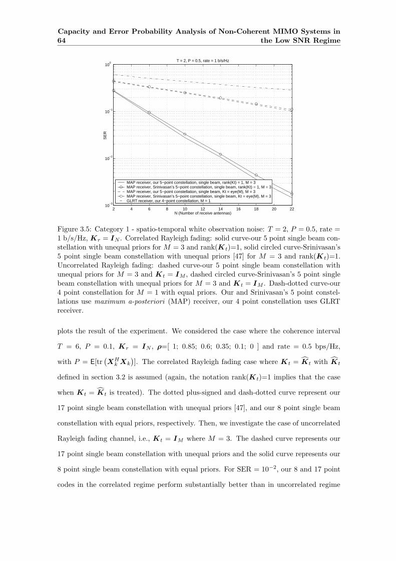
64Capacity and Error Probability Analysis of Non-Coherent MIMO Systems in
the Low SNR Regime
2 4 6 8 10 12 14 16 18 20 2210
−3
10−2
10−1
100
N (Number of receive antennas)
SE
R
T = 2, P = 0.5, rate = 1 b/s/Hz
MAP receiver, our 5−point constellation, single beam, rank(Kt) = 1, M = 3MAP receiver, Srinivasan’s 5−point constellation, single beam, rank(Kt) = 1, M = 3MAP receiver, our 5−point constellation, single beam, Kt = eye(M), M = 3MAP receiver, Srinivasan’s 5−point constellation, single beam, Kt = eye(M), M = 3GLRT receiver, our 4−point constellation, M = 1
Figure 3.5: Category 1 - spatio-temporal white observation noise: T = 2, P = 0.5, rate =1 b/s/Hz, Kr = IN . Correlated Rayleigh fading: solid curve-our 5 point single beam con-stellation with unequal priors for M = 3 and rank(K t)=1, solid circled curve-Srinivasan’s5 point single beam constellation with unequal priors [47] for M = 3 and rank(K t)=1.Uncorrelated Rayleigh fading: dashed curve-our 5 point single beam constellation withunequal priors for M = 3 and Kt = IM , dashed circled curve-Srinivasan’s 5 point singlebeam constellation with unequal priors for M = 3 and K t = IM . Dash-dotted curve-our4 point constellation for M = 1 with equal priors. Our and Srinivasan’s 5 point constel-lations use maximum a-posteriori (MAP) receiver, our 4 point constellation uses GLRTreceiver.
plots the result of the experiment. We considered the case where the coherence interval
T = 6, P = 0.1, Kr = IN , ρ=[ 1; 0.85; 0.6; 0.35; 0.1; 0 ] and rate = 0.5 bps/Hz,
with P = E[tr(XH
k Xk
)]. The correlated Rayleigh fading case where K t = Kt with Kt
defined in section 3.2 is assumed (again, the notation rank(K t)=1 implies that the case
when Kt = Kt is treated). The dotted plus-signed and dash-dotted curve represent our
17 point single beam constellation with unequal priors [47], and our 8 point single beam
constellation with equal priors, respectively. Then, we investigate the case of uncorrelated
Rayleigh fading channel, i.e., Kt = IM where M = 3. The dashed curve represents our
17 point single beam constellation with unequal priors and the solid curve represents our
8 point single beam constellation with equal priors. For SER = 10−2, our 8 and 17 point
codes in the correlated regime perform substantially better than in uncorrelated regime

3.3 Deterministic Fading Channel: the Low SNR PEP Analysis 65
(more than 10 receive antennas can be spared if one decides to make the transmit antennas
fully correlated). This is in concordance with the results presented in section 3.2 where
it has been proved that channel correlation can actually improve the performance of the
channel in arbitrary noise environment. We witness the effect of our 17 point codes losing
their superiority over 8 point codes as the number of receive antennas increases. This
can be justified by the fact that the signaling scheme proposed in [47] only resembles the
optimal, capacity achieving distribution.
0 2 4 6 8 10 12 14 16 1810
−3
10−2
10−1
100
N (Number of receive antennas)
SE
R
T = 8, K = 256, SNR = −10 dB, ρ = [ 1; 0.8; 0.5; 0.15; zeros(4,1) ]
GLRT receiver, M = 1, codes adapted to ρ = [ 1; 0.8; 0.5; 0.15; zeros(4,1) ]GLRT receiver, M = 2, codes adapted to ρ = [ 1; 0.8; 0.5; 0.15; zeros(4,1) ]GLRT receiver, M = 1, codes adapted to ρ = [ 1; zeros(7,1) ]GLRT receiver, M = 2, codes adapted to ρ = [ 1; zeros(7,1) ]
Figure 3.6: Category 2 - spatially white - temporally colored: T = 8, K = 256, SNR =-10 dB, ρ=[ 1; 0.8; 0.5; 0.15; zeros(4,1) ]. Solid curve-our codes for M = 1 adapted to ρ=[1; 0.8; 0.5; 0.15; zeros(4,1) ], solid-circled curve-our codes for M = 2 adapted to ρ=[ 1;0.8; 0.5; 0.15; zeros(4,1) ], dashed curve-our codes for M = 1 adapted to ρ=[ 1; zeros(7,1)], dashed-circled curve-our codes for M = 2 adapted to ρ=[ 1; zeros(7,1) ]. All codes useGLRT receiver.
Third category: E = s αT + Etemp
We considered the case where the noise matrix is of the form E = s αT + Etemp. This
models an interfering source s (with known covariance matrix Υs) where the complex
vector α is the known channel attenuation between each receive antenna and the interfering
source. The matrix Etemp has a noise covariance matrix belonging to the second category.
Thus, the noise covariance matrix is given by Υ = ααH ⊗Υs + IN ⊗ Σ(ρ). As in the
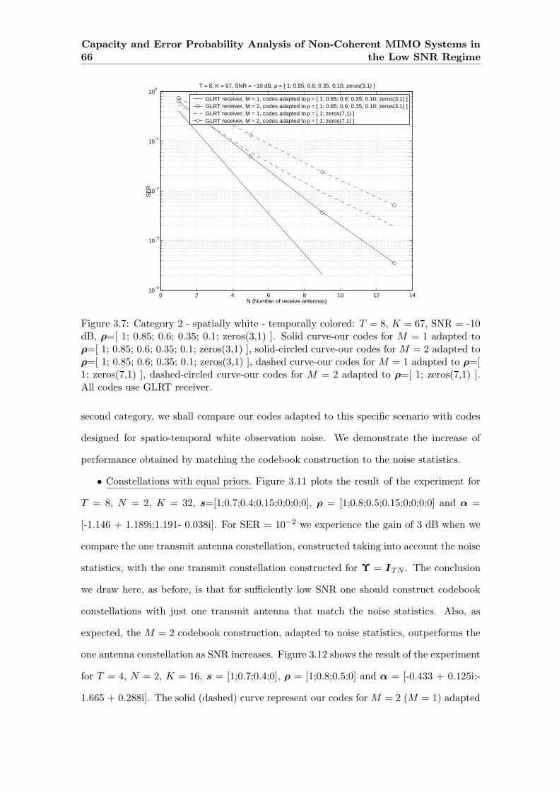
66Capacity and Error Probability Analysis of Non-Coherent MIMO Systems in
the Low SNR Regime
0 2 4 6 8 10 12 1410
−4
10−3
10−2
10−1
100
SE
R
N (Number of receive antennas)
T = 8, K = 67, SNR = −10 dB, ρ = [ 1; 0.85; 0.6; 0.35; 0.10; zeros(3,1) ]
GLRT receiver, M = 1, codes adapted to ρ = [ 1; 0.85; 0.6; 0.35; 0.10; zeros(3,1) ]GLRT receiver, M = 2, codes adapted to ρ = [ 1; 0.85; 0.6; 0.35; 0.10; zeros(3,1) ]GLRT receiver, M = 1, codes adapted to ρ = [ 1; zeros(7,1) ]GLRT receiver, M = 2, codes adapted to ρ = [ 1; zeros(7,1) ]
Figure 3.7: Category 2 - spatially white - temporally colored: T = 8, K = 67, SNR = -10dB, ρ=[ 1; 0.85; 0.6; 0.35; 0.1; zeros(3,1) ]. Solid curve-our codes for M = 1 adapted toρ=[ 1; 0.85; 0.6; 0.35; 0.1; zeros(3,1) ], solid-circled curve-our codes for M = 2 adapted toρ=[ 1; 0.85; 0.6; 0.35; 0.1; zeros(3,1) ], dashed curve-our codes for M = 1 adapted to ρ=[1; zeros(7,1) ], dashed-circled curve-our codes for M = 2 adapted to ρ=[ 1; zeros(7,1) ].All codes use GLRT receiver.
second category, we shall compare our codes adapted to this specific scenario with codes
designed for spatio-temporal white observation noise. We demonstrate the increase of
performance obtained by matching the codebook construction to the noise statistics.
• Constellations with equal priors. Figure 3.11 plots the result of the experiment for
T = 8, N = 2, K = 32, s=[1;0.7;0.4;0.15;0;0;0;0], ρ = [1;0.8;0.5;0.15;0;0;0;0] and α =
[-1.146 + 1.189i;1.191- 0.038i]. For SER = 10−2 we experience the gain of 3 dB when we
compare the one transmit antenna constellation, constructed taking into account the noise
statistics, with the one transmit constellation constructed for Υ = ITN . The conclusion
we draw here, as before, is that for sufficiently low SNR one should construct codebook
constellations with just one transmit antenna that match the noise statistics. Also, as
expected, the M = 2 codebook construction, adapted to noise statistics, outperforms the
one antenna constellation as SNR increases. Figure 3.12 shows the result of the experiment
for T = 4, N = 2, K = 16, s = [1;0.7;0.4;0], ρ = [1;0.8;0.5;0] and α = [-0.433 + 0.125i;-
1.665 + 0.288i]. The solid (dashed) curve represent our codes for M = 2 (M = 1) adapted
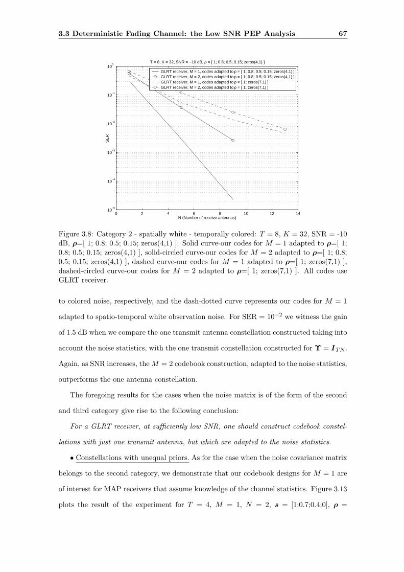
3.3 Deterministic Fading Channel: the Low SNR PEP Analysis 67
0 2 4 6 8 10 12 1410
−5
10−4
10−3
10−2
10−1
100
T = 8, K = 32, SNR = −10 dB, ρ = [ 1; 0.8; 0.5; 0.15; zeros(4,1) ]
N (Number of receive antennas)
SE
R
GLRT receiver, M = 1, codes adapted to ρ = [ 1; 0.8; 0.5; 0.15; zeros(4,1) ]GLRT receiver, M = 2, codes adapted to ρ = [ 1; 0.8; 0.5; 0.15; zeros(4,1) ]GLRT receiver, M = 1, codes adapted to ρ = [ 1; zeros(7,1) ]GLRT receiver, M = 2, codes adapted to ρ = [ 1; zeros(7,1) ]
Figure 3.8: Category 2 - spatially white - temporally colored: T = 8, K = 32, SNR = -10dB, ρ=[ 1; 0.8; 0.5; 0.15; zeros(4,1) ]. Solid curve-our codes for M = 1 adapted to ρ=[ 1;0.8; 0.5; 0.15; zeros(4,1) ], solid-circled curve-our codes for M = 2 adapted to ρ=[ 1; 0.8;0.5; 0.15; zeros(4,1) ], dashed curve-our codes for M = 1 adapted to ρ=[ 1; zeros(7,1) ],dashed-circled curve-our codes for M = 2 adapted to ρ=[ 1; zeros(7,1) ]. All codes useGLRT receiver.
to colored noise, respectively, and the dash-dotted curve represents our codes for M = 1
adapted to spatio-temporal white observation noise. For SER = 10−2 we witness the gain
of 1.5 dB when we compare the one transmit antenna constellation constructed taking into
account the noise statistics, with the one transmit constellation constructed for Υ = ITN .
Again, as SNR increases, the M = 2 codebook construction, adapted to the noise statistics,
outperforms the one antenna constellation.
The foregoing results for the cases when the noise matrix is of the form of the second
and third category give rise to the following conclusion:
For a GLRT receiver, at sufficiently low SNR, one should construct codebook constel-
lations with just one transmit antenna, but which are adapted to the noise statistics.
• Constellations with unequal priors. As for the case when the noise covariance matrix
belongs to the second category, we demonstrate that our codebook designs for M = 1 are
of interest for MAP receivers that assume knowledge of the channel statistics. Figure 3.13
plots the result of the experiment for T = 4, M = 1, N = 2, s = [1;0.7;0.4;0], ρ =
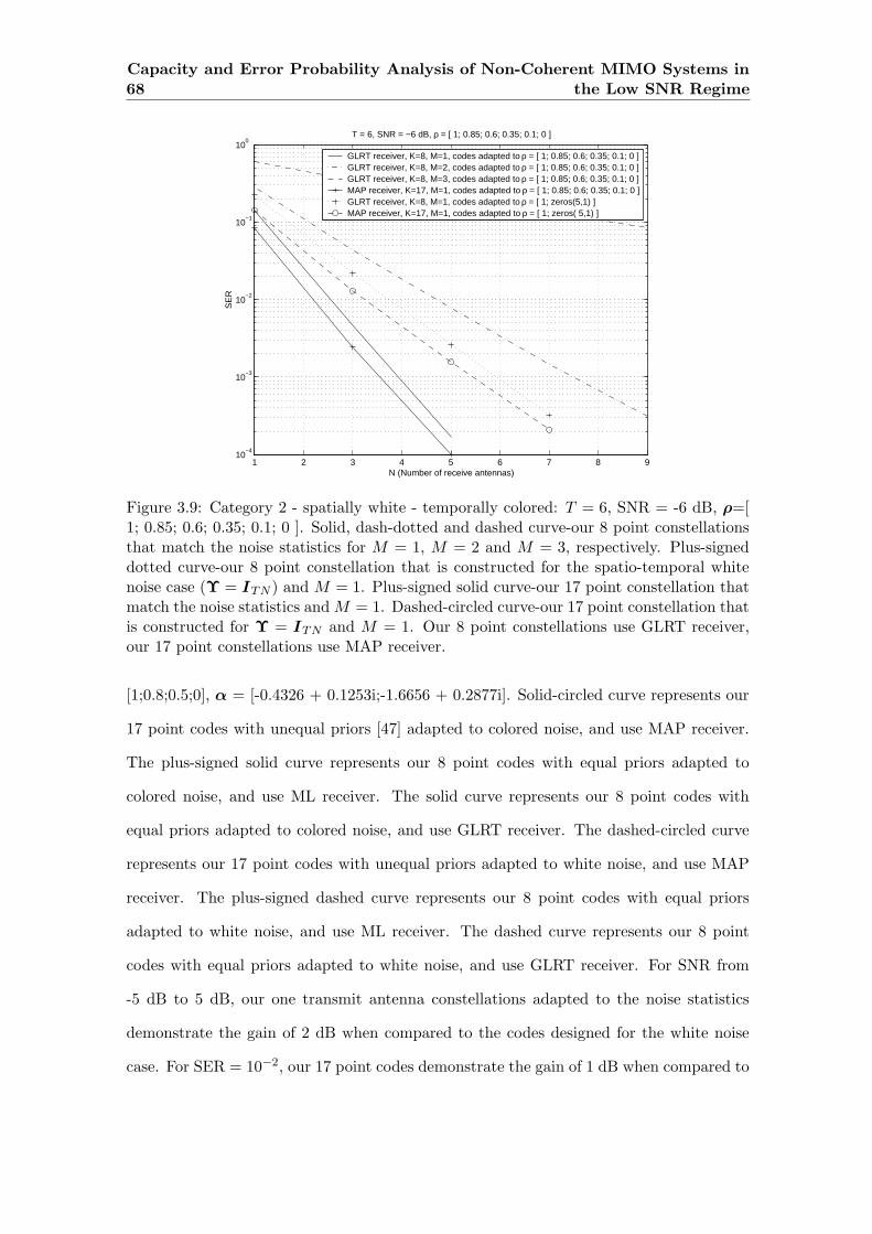
68Capacity and Error Probability Analysis of Non-Coherent MIMO Systems in
the Low SNR Regime
1 2 3 4 5 6 7 8 910
−4
10−3
10−2
10−1
100
T = 6, SNR = −6 dB, ρ = [ 1; 0.85; 0.6; 0.35; 0.1; 0 ]
N (Number of receive antennas)
SE
R
GLRT receiver, K=8, M=1, codes adapted to ρ = [ 1; 0.85; 0.6; 0.35; 0.1; 0 ]GLRT receiver, K=8, M=2, codes adapted to ρ = [ 1; 0.85; 0.6; 0.35; 0.1; 0 ]GLRT receiver, K=8, M=3, codes adapted to ρ = [ 1; 0.85; 0.6; 0.35; 0.1; 0 ]MAP receiver, K=17, M=1, codes adapted to ρ = [ 1; 0.85; 0.6; 0.35; 0.1; 0 ]GLRT receiver, K=8, M=1, codes adapted to ρ = [ 1; zeros(5,1) ]MAP receiver, K=17, M=1, codes adapted to ρ = [ 1; zeros( 5,1) ]
Figure 3.9: Category 2 - spatially white - temporally colored: T = 6, SNR = -6 dB, ρ=[1; 0.85; 0.6; 0.35; 0.1; 0 ]. Solid, dash-dotted and dashed curve-our 8 point constellationsthat match the noise statistics for M = 1, M = 2 and M = 3, respectively. Plus-signeddotted curve-our 8 point constellation that is constructed for the spatio-temporal whitenoise case (Υ = ITN ) and M = 1. Plus-signed solid curve-our 17 point constellation thatmatch the noise statistics and M = 1. Dashed-circled curve-our 17 point constellation thatis constructed for Υ = ITN and M = 1. Our 8 point constellations use GLRT receiver,our 17 point constellations use MAP receiver.
[1;0.8;0.5;0], α = [-0.4326 + 0.1253i;-1.6656 + 0.2877i]. Solid-circled curve represents our
17 point codes with unequal priors [47] adapted to colored noise, and use MAP receiver.
The plus-signed solid curve represents our 8 point codes with equal priors adapted to
colored noise, and use ML receiver. The solid curve represents our 8 point codes with
equal priors adapted to colored noise, and use GLRT receiver. The dashed-circled curve
represents our 17 point codes with unequal priors adapted to white noise, and use MAP
receiver. The plus-signed dashed curve represents our 8 point codes with equal priors
adapted to white noise, and use ML receiver. The dashed curve represents our 8 point
codes with equal priors adapted to white noise, and use GLRT receiver. For SNR from
-5 dB to 5 dB, our one transmit antenna constellations adapted to the noise statistics
demonstrate the gain of 2 dB when compared to the codes designed for the white noise
case. For SER = 10−2, our 17 point codes demonstrate the gain of 1 dB when compared to
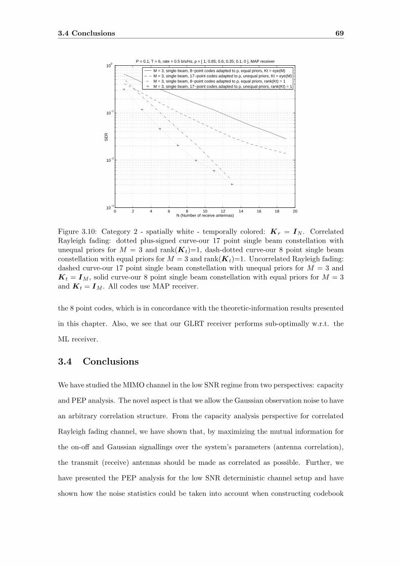
3.4 Conclusions 69
0 2 4 6 8 10 12 14 16 18 2010
−3
10−2
10−1
100
P = 0.1, T = 6, rate = 0.5 b/s/Hz, ρ = [ 1; 0.85; 0.6; 0.35; 0.1; 0 ], MAP receiver
N (Number of receive antennas)
SE
R
M = 3, single beam, 8−point codes adapted to ρ, equal priors, Kt = eye(M)M = 3, single beam, 17−point codes adapted to ρ, unequal priors, Kt = eye(M)M = 3, single beam, 8−point codes adapted to ρ, equal priors, rank(Kt) = 1M = 3, single beam, 17−point codes adapted to ρ, unequal priors, rank(Kt) = 1
Figure 3.10: Category 2 - spatially white - temporally colored: Kr = IN . CorrelatedRayleigh fading: dotted plus-signed curve-our 17 point single beam constellation withunequal priors for M = 3 and rank(K t)=1, dash-dotted curve-our 8 point single beamconstellation with equal priors for M = 3 and rank(K t)=1. Uncorrelated Rayleigh fading:dashed curve-our 17 point single beam constellation with unequal priors for M = 3 andKt = IM , solid curve-our 8 point single beam constellation with equal priors for M = 3and Kt = IM . All codes use MAP receiver.
the 8 point codes, which is in concordance with the theoretic-information results presented
in this chapter. Also, we see that our GLRT receiver performs sub-optimally w.r.t. the
ML receiver.
3.4 Conclusions
We have studied the MIMO channel in the low SNR regime from two perspectives: capacity
and PEP analysis. The novel aspect is that we allow the Gaussian observation noise to have
an arbitrary correlation structure. From the capacity analysis perspective for correlated
Rayleigh fading channel, we have shown that, by maximizing the mutual information for
the on-off and Gaussian signallings over the system’s parameters (antenna correlation),
the transmit (receive) antennas should be made as correlated as possible. Further, we
have presented the PEP analysis for the low SNR deterministic channel setup and have
shown how the noise statistics could be taken into account when constructing codebook
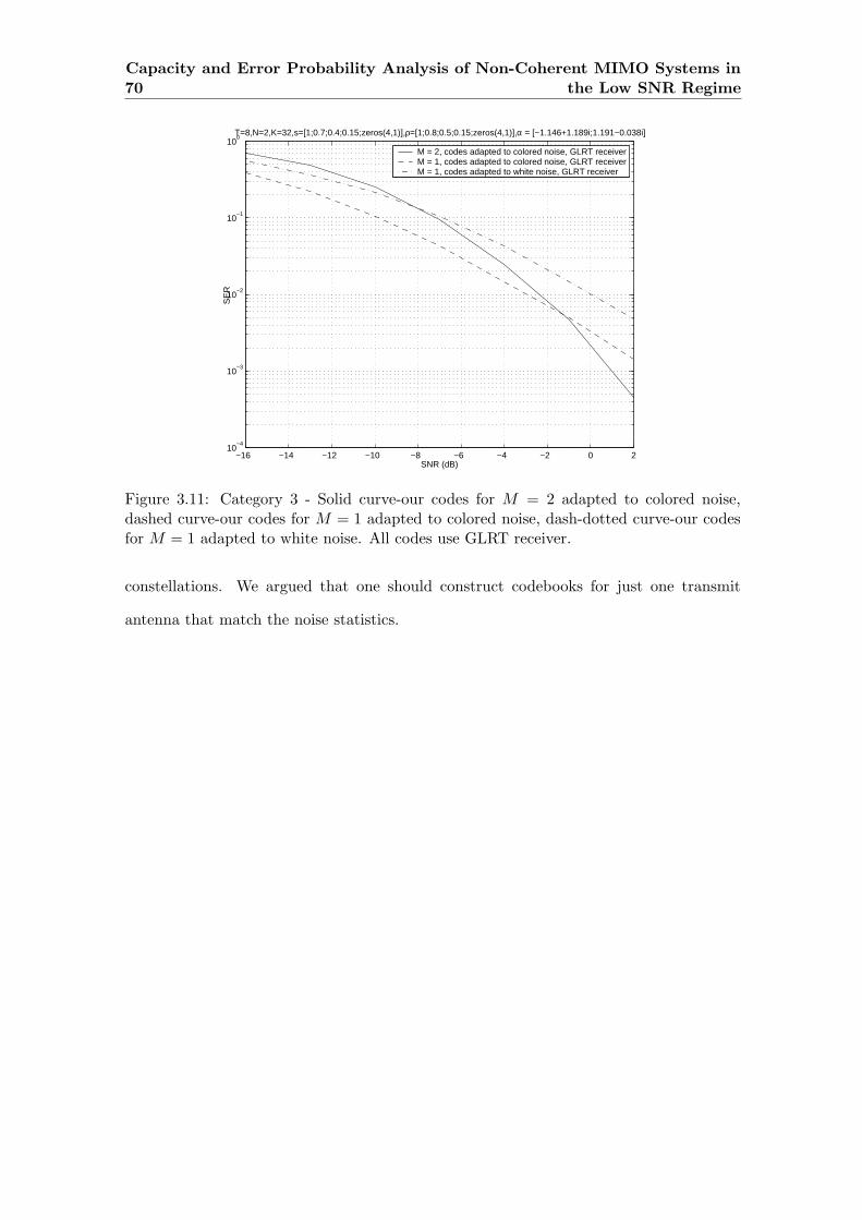
70Capacity and Error Probability Analysis of Non-Coherent MIMO Systems in
the Low SNR Regime
−16 −14 −12 −10 −8 −6 −4 −2 0 210
−4
10−3
10−2
10−1
100
SNR (dB)
SE
R
T=8,N=2,K=32,s=[1;0.7;0.4;0.15;zeros(4,1)],ρ=[1;0.8;0.5;0.15;zeros(4,1)],α = [−1.146+1.189i;1.191−0.038i]
M = 2, codes adapted to colored noise, GLRT receiverM = 1, codes adapted to colored noise, GLRT receiverM = 1, codes adapted to white noise, GLRT receiver
Figure 3.11: Category 3 - Solid curve-our codes for M = 2 adapted to colored noise,dashed curve-our codes for M = 1 adapted to colored noise, dash-dotted curve-our codesfor M = 1 adapted to white noise. All codes use GLRT receiver.
constellations. We argued that one should construct codebooks for just one transmit
antenna that match the noise statistics.
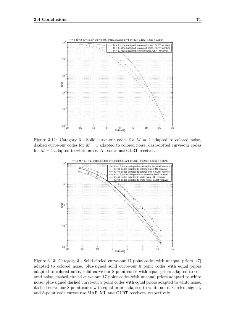
3.4 Conclusions 71
−20 −15 −10 −5 0 5 10 15 2010
−5
10−4
10−3
10−2
10−1
100
SNR (dB)
SE
R
T = 4, N = 2, K = 16, s=[1;0.7;0.4;0], ρ=[1;0.8;0.5;0], α = [−0.433 + 0.125i;−1.665 + 0.288i]
M = 2, codes adapted to colored noise, GLRT receiver M = 1, codes adapted to colored noise, GLRT receiverM = 1, codes adapted to white noise, GLRT receiver
Figure 3.12: Category 3 - Solid curve-our codes for M = 2 adapted to colored noise,dashed curve-our codes for M = 1 adapted to colored noise, dash-dotted curve-our codesfor M = 1 adapted to white noise. All codes use GLRT receiver.
−20 −15 −10 −5 0 5 10 1510
−4
10−3
10−2
10−1
100
SNR (dB)
SE
R
T = 4, M = 1,N = 2, s=[1;0.7;0.4;0], ρ=[1;0.8;0.5;0], α=[−0.4326 + 0.1253i;−1.6656 + 0.2877i]
K = 17, codes adapted to colored noise, MAP receiverK = 8, codes adapted to colored noise, ML receiverK = 8, codes adapted to colored noise, GLRT receiverK = 17, codes adapted to white noise, MAP receiverK = 8, codes adapted to white noise, ML receiverK = 8, codes adapted to white noise, GLRT receiver
Figure 3.13: Category 3 - Solid-circled curve-our 17 point codes with unequal priors [47]adapted to colored noise, plus-signed solid curve-our 8 point codes with equal priorsadapted to colored noise, solid curve-our 8 point codes with equal priors adapted to col-ored noise, dashed-circled curve-our 17 point codes with unequal priors adapted to whitenoise, plus-signed dashed curve-our 8 point codes with equal priors adapted to white noise,dashed curve-our 8 point codes with equal priors adapted to white noise. Circled, signed,and 8-point code curves use MAP, ML and GLRT receivers, respectively.

72Capacity and Error Probability Analysis of Non-Coherent MIMO Systems in
the Low SNR Regime

Chapter 4
Conclusions and Future Work
4.1 Conclusions
The research conducted in this thesis can be divided in two parts: high and low SNR
regime.
In Chapter 2, we addressed the problem of space-time codebook design for non-coherent
communications in multiple-antenna wireless systems and high SNR regime. In contrast
with other approaches, the channel matrix was modeled as an unknown deterministic
parameter at both the receiver and the transmitter, and the Gaussian observation noise
was allowed to have an arbitrary correlation structure, known by the transmitter and
the receiver. In order to handle the unknown deterministic space-time channel, a GLRT
receiver was considered. A new methodology for space-time codebook design under this
non-coherent setup was proposed. This optimizes the probability of error of the GLRT
receiver’s detector in the high SNR regime, thus solving a high-dimensional nonlinear non-
smooth optimization problem in a two-step approach: (i) firstly, a convex SDP relaxation
of the codebook design problem yields a rough estimate of the optimal codebook; (ii) this
is then refined through a geodesic descent optimization algorithm that exploits the Rie-
mannian geometry imposed by the power constraints on the space-time codewords. The
results obtained through computer simulations illustrate the advantages of our method.
For the specific case of spatio-temporal white observation noise, our codebook construc-
tions replicate the performance of state-of-art known solutions. The main point here is
that our methodology permits to extend the codebook construction to any given corre-
lated noise environment. The simulation results show the good performance of these new
73

74 Conclusions and Future Work
designed codes in colored noise setups.
In Chapter 3, the non-coherent single-user MIMO channel in the low SNR regime
was investigated from two viewpoints: capacity and probability of error analysis. The
novelty in both viewpoints is that an arbitrary correlation structure is allowed for the
Gaussian observation noise. First, we looked at the capacity of the spatially correlated
Rayleigh fading channel. We investigated the impact of channel and noise correlation
on the mutual information for the on-off and Gaussian signaling schemes. Our results
establish that, in the low SNR regime, mutual information is maximized when the transmit
antennas are fully correlated (the same holds for the receive array). Then, we considered
the deterministic channel setup and perform a PEP analysis for the GLRT receiver. This
leads to a codebook design criterion on which we base the construction of new space-time
constellations. Their performance were assessed by computer simulations and we argued
that one should construct codebooks for just one transmit antenna that match the noise
statistics. As a byproduct, we showed that our codebooks are also of interest for Bayesian
receivers which decode constellations with non-uniform priors.
4.2 Future Work
There are number of possibilities for future research. In the following, some research
directions are mentioned:
1. An important outcome of this thesis is the conclusion that is worthwhile to treat the
codebook design problem in the case when the Gaussian observation noise is allowed
to have an arbitrary correlation structure, since we have seen that if the perfect
knowledge of the noise correlation is available, significant improvements over uni-
tary constellations in general correlated noise environments are possible. Potential
next questions to consider are the following. The designed codebooks do not possess
any structure that could alleviate a reduction in the size of the memory needed to
store them. This is especially important in the high SNR regime where, due to large
capacity, one should construct high-rate constellations. (In the low-medium SNR
regime, constellations with relatively small cardinalities suffice since the channel ca-

4.2 Future Work 75
pacities are also relatively small). In practice, the storage of a high-rate unstructured
codebook becomes infeasible because the size of the codebook increases exponentially
with the data rate. Hence, the design of structured constellations, which will con-
sequently allow tractable encoding, may be a topic for future research. Likewise,
there is a concern w.r.t. the decoding complexity. The decoding complexity of the
codebook constructions is, unfortunately, exponential in the data rate. Since, in
this work, the decoding complexity did not represent a constraint, the design of
non-coherent STC with reduced complexity algorithms remains an important open
problem that deserves further investigation.
2. Throughout the thesis, the noise covariance matrix is assumed to be perfectly known
at the site where the codebook design is performed. An assessment of the sensitivity
of the codebook design to mismatch between the noise covariance assumed in the
design and the noise covariance encountered in practice could be a good topic for
future work.
3. The research presented in the thesis has been conducted on channels that are as-
sumed to be flat fading. This can be considered true for low symbol rate or narrow
bandwidth communications systems. For higher symbol rate transmissions, fading
is frequency selective and so poses a greater challenge given limited link budget and
severity of wireless environment. We plan to devote our attention to orthogonal
frequency division multiplexing (OFDM) which has emerged as a very promising
technique to provide high data-rate transmission over broadband MIMO channels.
Its relevance is testified by being chosen as the standard interface for digital audio
broadcasting (DAB), terrestrial digital video broadcasting (DVB), wireless local area
networks (WLANs), and wireless metropolitan area networks (MANs). One of the
key advantages of OFDM over traditional single-carrier modulation and CDMA is
its low computational complexity in practical implementations. MIMO-OFDM is
therefore a particularly promising candidate for future fourth-generation (4G) wire-
less networks. An interesting research direction is the design of optimum modulation
76 Conclusions and Future Work
and coding schemes for MIMO-OFDM in both high and low SNR regime. We are
particularly interested in the non-coherent case. Our goal is to find modulation and
coding schemes for MIMO-OFDM that exploit the available spatial and frequency
diversity, being robust for a wide range of realistic channels.
4. In Chapter 2, new packings in the complex projective space have been presented. In
some cases we were able to construct optimal packings that meet the Rankin bound
(so-called ETFs). Equivalently, an ETF can be seen as a sequence of K unit vectors
in a T -dimensional Euclidian space whose pairwise absolute inner products meet the
well-known Welch lower bound [65]. ETFs have applications in communications,
coding theory and sparse approximation [78], [79]. As an example, in [80] it has
been shown that an ETF provides an error correcting code that is maximally robust
against two erasures. ETFs also play an important role in multiuser communication
systems. It is known that ETFs achieve the capacity of a Gaussian channel and
satisfy an interference invariance property [81]. Numerical evidence indicates that
complex ETFs do not exist for most pairs (T, K). An interesting open question is
to find conditions on (T, K) that rule out the existence of general complex ETFs.
In the other direction, it seems that a maximal complex ETF exists for each natural
number T (in this specific case K = T 2). Resolving this conjecture represents a
challenging topic for future work.
5. In Chapter 3, section 3.2, the capacity analysis of MIMO fading channels in the
low SNR regime for the case when the channel correlation matrix is modeled by
the Kronecker product of the transmit and receive correlation matrix was presented.
The generalization of the analysis to the case when the channel covariance matrix
has an arbitrary correlation structure represents a possible topic for future work.
Moreover, an extension of the analysis presented in Chapter 3 to the cases when
peak and fourth-order moment signal constraints are imposed in order to determine
what signaling should be applied to the input, how many transmit antennas should
be employed and what is the optimal value of the channel covariance matrix is an

4.2 Future Work 77
interesting topic for future research.

78 Conclusions and Future Work

Appendix A
Pairwise Error Probability for Fast
Fading in the High SNR Regime
In this appendix, we derive the expression for the asymptotic (high SNR regime) pairwise
error probability for fast fading presented in (2.8).
If Xi is transmitted, then the probability that the receiver decides in favor of X j is:
PXi→Xj= P (zH
i Υ−1zi > zHj Υ−1zj) (A.1)
where for k ∈ i, j
zk = y − Xkgk,
Xk = IN ⊗Xk, X k = Υ− 1
2 Xk
y = vec(Y ) = Xig + e, e = vec(E),
and
gk = (X Hk X k)
−1X Hk Υ− 1
2 y
is the ML estimate of the channel when Xk is transmitted. The unknown realization of
the channel is denoted by g = vec(HH).
Let Si = (X Hi X i)
−1X Hi Υ− 1
2 . Thus,
zi = y − Xigi
= (ITN − XiSi)︸ ︷︷ ︸P i
(Xig + e)
= P ie. (A.2)
79

80 Pairwise Error Probability for Fast Fading in the High SNR Regime
Similarly, it can be shown that
zj = ∆g + P je (A.3)
where P j = ITN − XjSj and ∆ = P jXi. Hence, substituting (A.2) and (A.3) in (A.1)
we have
PXi→Xj= P (eH(P H
i Υ−1P i − P Hj Υ−1P j︸ ︷︷ ︸
T
)e−
− eHP Hj Υ−1∆g − gH∆HΥ−1P je > gH∆HΥ−1∆g︸ ︷︷ ︸
λ
). (A.4)
Unfortunately, the expression (A.4) cannot be simplified analytically. We shall an-
alyze (A.4) in the high SNR regime where the linear term of e is dominant, i.e., the
quadratic term of e is negligible. In the following, we explain better the preceding claim.
First note that SNR and Υ are linked by the formula
SNR =E[∥∥XkH
H∥∥2]
E[‖E‖2
] =tr(HHHE
[XH
k Xk
])
tr (Υ).
In the above equation, the channel was assumed deterministic (we used assumption A1.).
Moreover, once the codebook is fixed, we have E[XH
k Xk
]= R for a certain positive-
definite matrix R. Thus,
SNR =κ
tr (Υ), κ := tr
(HHHR
),
and saying that SNR → +∞ corresponds to saying that Υ → 0. Our argument is that
when SNR → +∞ the linear term
z = −eHP Hj Υ−1∆g − gH∆HΥ−1P je
dominates (in the mean square sense) the quadratic term eT Te in (A.4).
As the random vector e ∼ CN (0,Υ) and other quantities in (A.4), e.g., P j , ∆, depend
on Υ we admit that our claim is not readily acceptable. However, if we work out the
dependencies, it can be validated. We propose the following exercise. Let Υ = Υ(t) = tΥ0
for some (fixed) Hermitian positive definite matrix Υ0 and t > 0. Taking t ↓ 0 corresponds
to making SNR → +∞. Remark that
ed= Υ1/2z

81
whered= means equality in distribution and z ∼ CN (0, ITN ). Now, if we unwind the
definitions of P j , etc, and go through tedious but straightforward computations, it can be
seen that (A.4) boils down to
PXi→Xj= P
(zHCz − 1√
t
(zHc + cHz
)>
1
tη
)(A.5)
where C, c and η denote constants with respect to t (they do not depend on t) which are
not explicitly given here. Thus, the random variables
zHCz and zHc + cHz
have fixed power (not depending on t, i.e., SNR). Since t > 0 we can rewrite (A.5) as
PXi→Xj= P
(tzHCz −
√t(zHc + cHz
)> η
). (A.6)
When t ↓ 0 (SNR → +∞) we have t √
t and that’s how we justify the approximation
PXi→Xj≈ P
(−√
t(zHc + cHz
)> η
)(A.7)
which corresponds to (A.6) above. As a side remark, note that (A.7) confirms that
PXi→Xj→ 0 as t ↓ 0, thanks to the fact that η > 0.
The above argument is not new. We were inspired by similar manipulations from the
book [19], see pp. 56.
Therefore,
PXi→Xj≈ P (−eHP H
j Υ−1∆g − gH∆HΥ−1P je︸ ︷︷ ︸z
> λ). (A.8)
We see that z is a real Gaussian variable with zero mean (because E[e] = 0) and
unknown variance σ2, i.e., ziid∼ N
(0, σ2
), which will be calculated in sequel:
σ2 = E[z2] = E[(eHP H
j Υ−1∆g + gH∆HΥ−1P je)2
]
= E[gH∆HΥ−1P jeeHP Hj Υ−1∆g + eHP H
j Υ−1∆ggH∆HΥ−1P je].
Continuing with analysis,
E[eHP Hj Υ−1∆ggH∆HΥ−1P je] = tr
(E[eeHP H
j Υ−1∆ggH∆HΥ−1P j ])
= gH∆HΥ−1P jΥP Hj Υ−1∆g
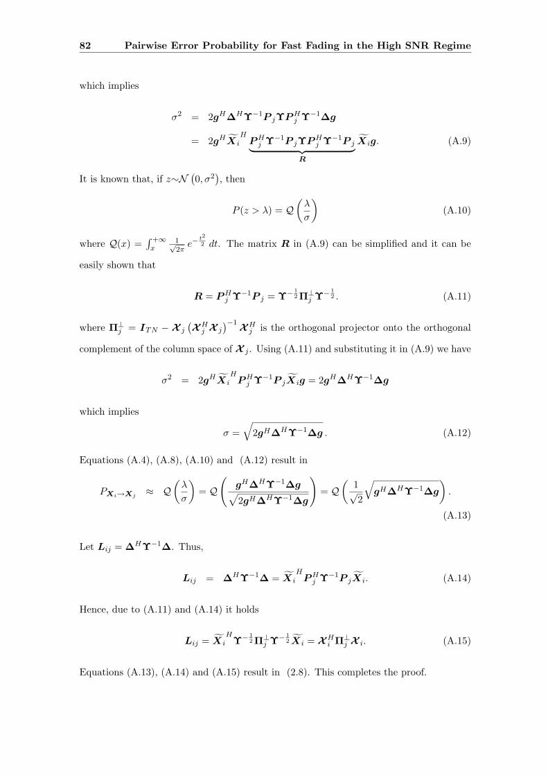
82 Pairwise Error Probability for Fast Fading in the High SNR Regime
which implies
σ2 = 2gH∆HΥ−1P jΥP Hj Υ−1∆g
= 2gHXiH
P Hj Υ−1P jΥP H
j Υ−1P j︸ ︷︷ ︸R
Xig. (A.9)
It is known that, if z∼N(0, σ2
), then
P (z > λ) = Q(
λ
σ
)(A.10)
where Q(x) =∫ +∞x
1√2π
e−t2
2 dt. The matrix R in (A.9) can be simplified and it can be
easily shown that
R = P Hj Υ−1P j = Υ− 1
2 Π⊥j Υ− 1
2 . (A.11)
where Π⊥j = ITN − X j
(X H
j X j
)−1X H
j is the orthogonal projector onto the orthogonal
complement of the column space of X j . Using (A.11) and substituting it in (A.9) we have
σ2 = 2gHXiH
P Hj Υ−1P jXig = 2gH∆HΥ−1∆g
which implies
σ =
√2gH∆HΥ−1∆g . (A.12)
Equations (A.4), (A.8), (A.10) and (A.12) result in
PXi→Xj≈ Q
(λ
σ
)= Q
(gH∆HΥ−1∆g√2gH∆HΥ−1∆g
)= Q
(1√2
√gH∆HΥ−1∆g
).
(A.13)
Let Lij = ∆HΥ−1∆. Thus,
Lij = ∆HΥ−1∆ = XiH
P Hj Υ−1P jXi. (A.14)
Hence, due to (A.11) and (A.14) it holds
Lij = XiHΥ− 1
2 Π⊥j Υ− 1
2 Xi = X Hi Π⊥
j X i. (A.15)
Equations (A.13), (A.14) and (A.15) result in (2.8). This completes the proof.

Appendix B
Optimization Problem
In this section, we prove that the equivalent formulation of the optimization problem (2.36)
is given by (2.37).
The optimization problem in (2.36) can be rewritten in the following way
(X∗
k, t∗) = arg max
λmin(Lmk) ≥ t,m = 1, ..., k − 1 (A)
λmin(Lkm) ≥ t,m = 1, ..., k − 1 (B)
tr(XH
kXk) = 1,
t (B.1)
where
Lij = X Hi Π⊥
j X i, Π⊥j = ITN −X j(X
Hj X j)
−1X Hj ,
X i = Υ− 1
2 Xi and Xi = IN ⊗X i.
Approach: Define Xk = vec(Xk)vecH(Xk). We are going to show that both (A) and
(B) can be written as LMI’s with respect to Xk, vec(Xk) and t.
(A) Note that
λmin(Lmk) ≥ t ⇔ Lmk − tIMN 0.
Since the matrix Lmk− tIMN = X HmX m−X H
mX k(XHk X k)
−1X Hk X m− tIMN is the Schur
complement [84] of X Hk X k in
[X H
k X k X Hk X m
X HmX k X H
mX m − tIMN
]
we have the following equivalence (we assumed that Xk is of full column rank):
λmin(Lmk) ≥ t ⇔[X H
k X k X Hk X m
X HmX k X H
mX m − tIMN
] 0. (B.2)
83

84 Optimization Problem
• Let [M ]i,j denote the ij-th element of the matrix M and ei represent the i-th column
of the identity matrix IMN . Then,
[X Hk X k]i,j = eH
i X Hk X kej = eH
i XkHΥ−1Xkej = tr
(Υ−1Xkej
(Xkei
)H)
(B.3)
As Xk = IN ⊗ Xk, there exists matrix K of size TMN 2 × TM such that vec(Xk) =
K vec(Xk), see [90]. Hence,
Xkej = vec(Xkej
)=(eT
j ⊗ ITN
)vec(Xk) = (eT
j ⊗ ITN )Kvec(Xk). (B.4)
Substituting (B.4) in (B.3) we have
[X Hk X k]i,j = tr
(Υ−1(eT
j ⊗ ITN )Kvec(Xk)((eT
i ⊗ ITN )Kvec(Xk))H)
= tr (Bij (ITN ) Xk) , (B.5)
where we define Bij(Φ) = KH(ei ⊗ ITN )Υ− 1
2 ΦΥ− 1
2 (eTj ⊗ ITN )K.
• Similarly,
[X HmX k]i,j = eH
i X HmX kej = eH
i X HmΥ− 1
2 Xkej = eHi X H
mΥ− 1
2 (eTj ⊗ ITN )K vec(Xk).
(B.6)
(B) By repeating the analysis for the case (A) we have:
[Lkm]i,j = eHi X H
k Π⊥mX kej = eH
i XkHΥ− 1
2 Π⊥mΥ− 1
2 Xkej
= tr
(Υ− 1
2 Π⊥mΥ− 1
2 Xkej
(Xkei
)H)
.
Using (B.4) we obtain
[Lkm]i,j = tr(KH(ei ⊗ ITN )Υ− 1
2 Π⊥mΥ− 1
2 (eTj ⊗ ITN )Kvec(Xk)vecH(Xk)
).
Hence,
[Lkm]i,j = tr(Bij(Π
⊥m) Xk
). (B.7)
Combining (B.2), (B.3), (B.5), (B.6) and (B.7) we conclude that both (A) and (B) can
be written as LMI’s with respect to the variables Xk, vec(Xk) and t. Consequently, the
optimization problems (2.36) and (2.37) are equivalent. This concludes the proof.
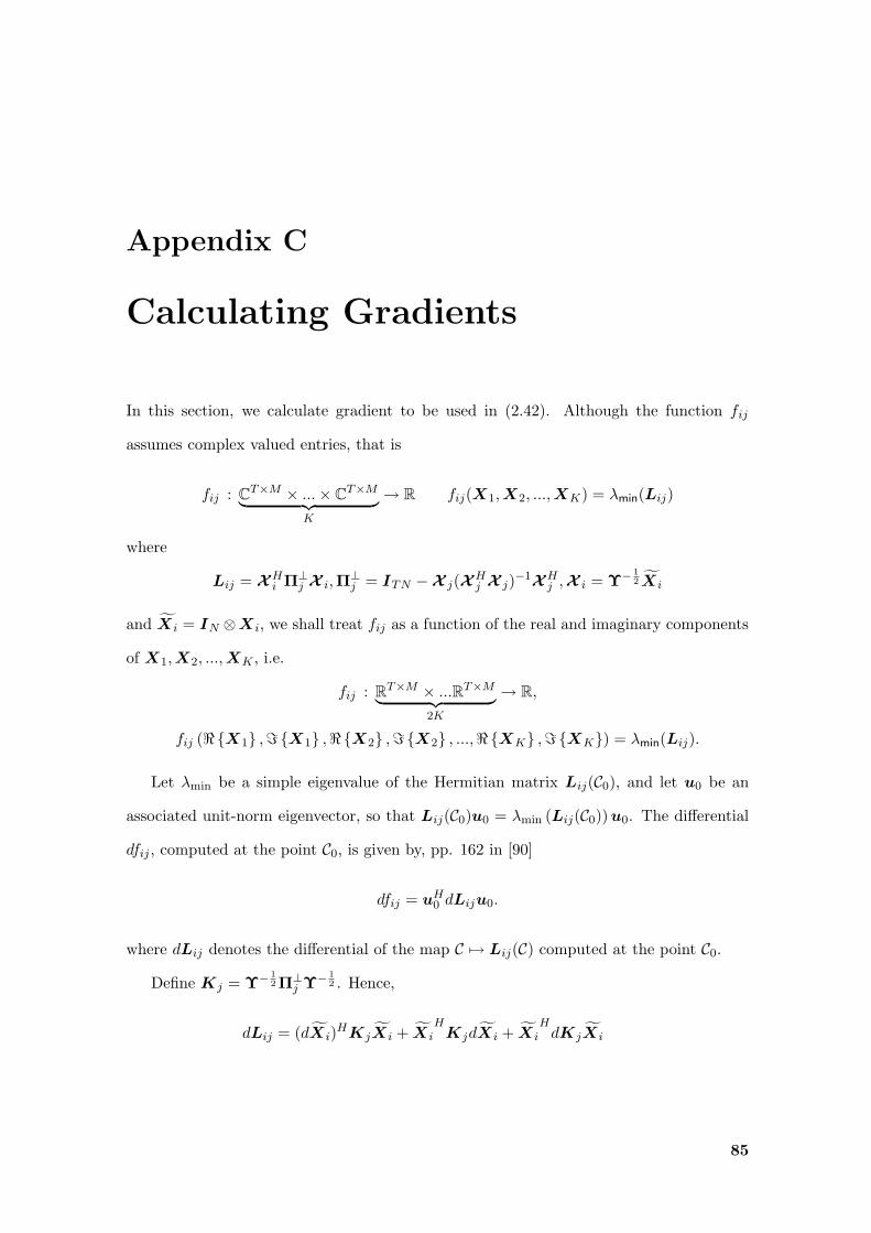
Appendix C
Calculating Gradients
In this section, we calculate gradient to be used in (2.42). Although the function fij
assumes complex valued entries, that is
fij : CT×M × ...× C
T×M︸ ︷︷ ︸
K
→ R fij(X1, X2, ..., XK) = λmin(Lij)
where
Lij = X Hi Π⊥
j X i,Π⊥j = ITN −X j(X
Hj X j)
−1X Hj , X i = Υ− 1
2 Xi
and Xi = IN ⊗X i, we shall treat fij as a function of the real and imaginary components
of X1, X2, ..., XK , i.e.
fij : RT×M × ...RT×M︸ ︷︷ ︸
2K
→ R,
fij (<X1 ,=X1 ,<X2 ,=X2 , ...,<XK ,=XK) = λmin(Lij).
Let λmin be a simple eigenvalue of the Hermitian matrix Lij(C0), and let u0 be an
associated unit-norm eigenvector, so that Lij(C0)u0 = λmin (Lij(C0)) u0. The differential
dfij , computed at the point C0, is given by, pp. 162 in [90]
dfij = uH0 dLiju0.
where dLij denotes the differential of the map C 7→ Lij(C) computed at the point C0.
Define Kj = Υ− 1
2 Π⊥j Υ− 1
2 . Hence,
dLij = (dXi)HKjXi + Xi
HKjdXi + Xi
HdKjXi
85
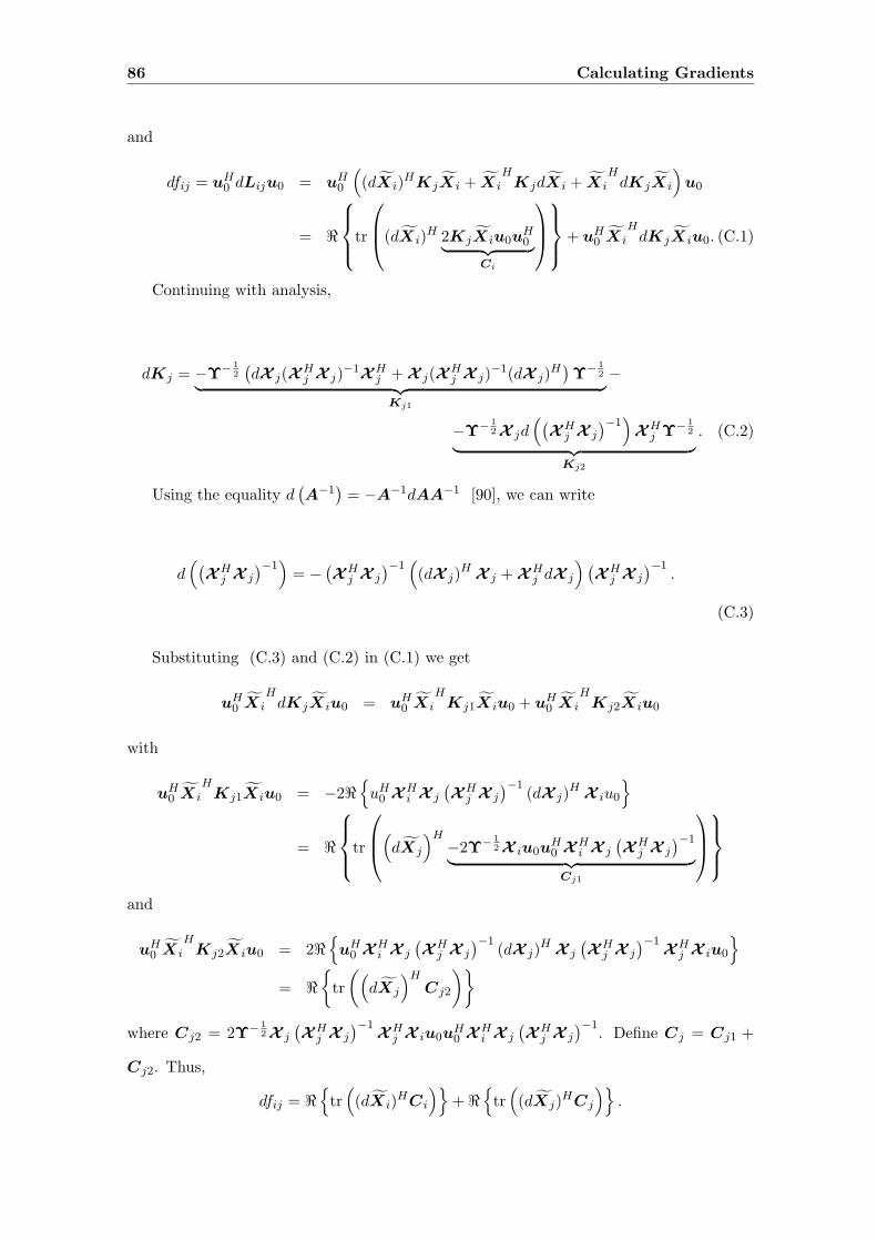
86 Calculating Gradients
and
dfij = uH0 dLiju0 = uH
0
((dXi)
HKjXi + XiH
KjdXi + XiH
dKjXi
)u0
= <
tr
(dXi)
H 2KjXiu0uH0︸ ︷︷ ︸
Ci
+ uH0 Xi
HdKjXiu0. (C.1)
Continuing with analysis,
dKj = −Υ− 1
2
(dX j(X
Hj X j)
−1X Hj + X j(X
Hj X j)
−1(dX j)H)Υ− 1
2
︸ ︷︷ ︸Kj1
−
−Υ− 1
2 X jd((
X Hj X j
)−1)
X Hj Υ− 1
2
︸ ︷︷ ︸Kj2
. (C.2)
Using the equality d(A−1
)= −A−1dAA−1 [90], we can write
d((
X Hj X j
)−1)
= −(X H
j X j
)−1((dX j)
HX j + X H
j dX j
) (X H
j X j
)−1.
(C.3)
Substituting (C.3) and (C.2) in (C.1) we get
uH0 Xi
HdKjXiu0 = uH
0 XiH
Kj1Xiu0 + uH0 Xi
HKj2Xiu0
with
uH0 Xi
HKj1Xiu0 = −2<
uH
0 X Hi X j
(X H
j X j
)−1(dX j)
HX iu0
= <
tr
(dXj
)H−2Υ− 1
2 X iu0uH0 X H
i X j
(X H
j X j
)−1
︸ ︷︷ ︸Cj1
and
uH0 Xi
HKj2Xiu0 = 2<
uH
0 X Hi X j
(X H
j X j
)−1(dX j)
HX j
(X H
j X j
)−1X H
j X iu0
= <
tr
((dXj
)HCj2
)
where Cj2 = 2Υ− 1
2 X j
(X H
j X j
)−1X H
j X iu0uH0 X H
i X j
(X H
j X j
)−1. Define Cj = Cj1 +
Cj2. Thus,
dfij = <
tr((dXi)
HCi
)+ <
tr((dXj)
HCj
).
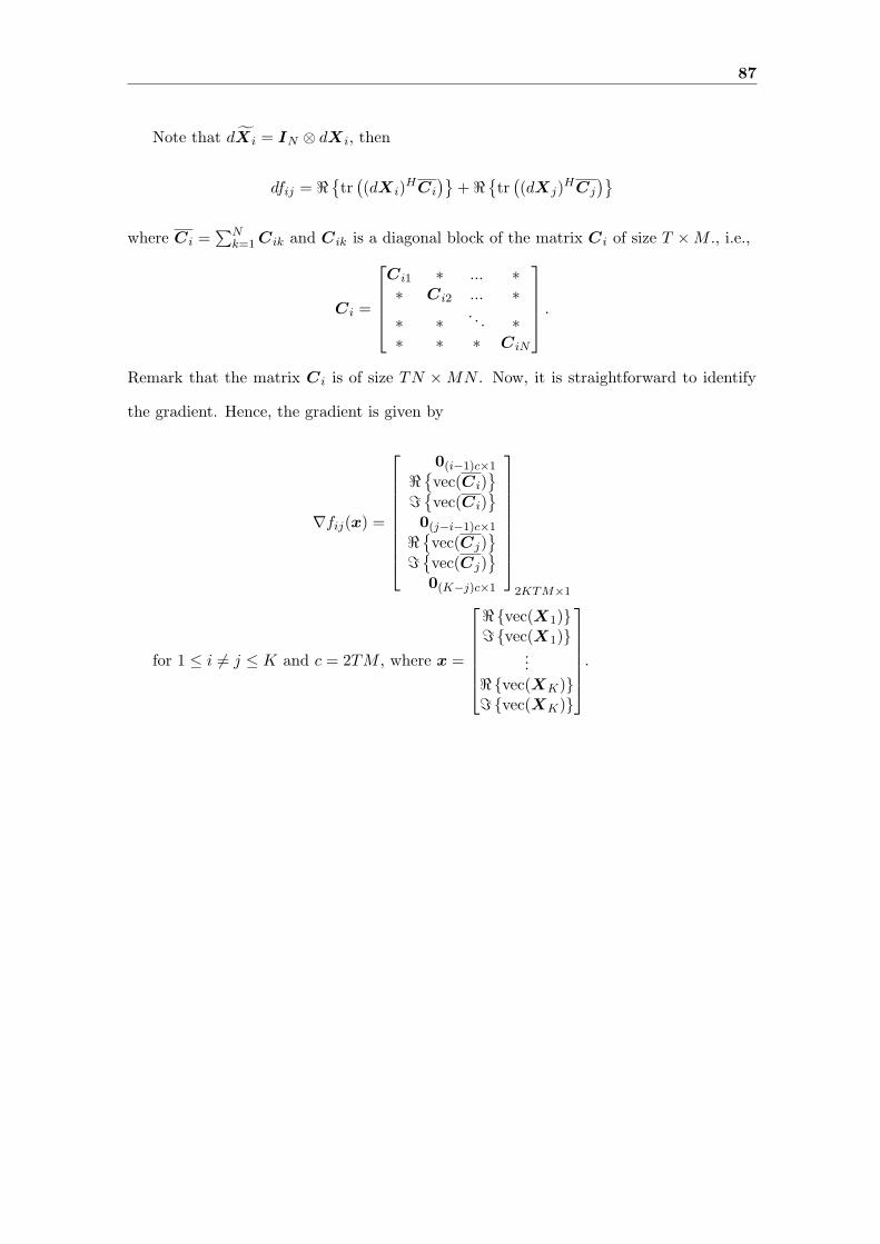
87
Note that dXi = IN ⊗ dX i, then
dfij = <tr((dX i)
HCi
)+ <
tr((dXj)
HCj
)
where Ci =∑N
k=1 Cik and Cik is a diagonal block of the matrix C i of size T ×M ., i.e.,
Ci =
Ci1 ∗ ... ∗∗ Ci2 ... ∗∗ ∗ . . . ∗∗ ∗ ∗ CiN
.
Remark that the matrix C i is of size TN ×MN . Now, it is straightforward to identify
the gradient. Hence, the gradient is given by
∇fij(x) =
0(i−1)c×1
<vec(Ci)
=vec(Ci)
0(j−i−1)c×1
<vec(Cj)
=vec(Cj)
0(K−j)c×1
2KTM×1
for 1 ≤ i 6= j ≤ K and c = 2TM , where x =
<vec(X1)= vec(X1)
...<vec(XK)= vec(XK)
.

88 Calculating Gradients
Appendix D
Mutual Information for On-Off
Signaling in the Low SNR Regime
In this section, we show that the expression for the mutual information between Y and
X up to first order in ρ, for on-off signaling and sufficiently low SNR, is given by (3.2).
Since
I(Y ; X) = h(Y )− h(Y |X),
we shall find the mutual information by computing the conditional entropy of Y given X,
i.e., h(Y |X), and in sequel, the entropy of Y , i.e., h(Y ).
• We start by computing h(Y |X). Given X, y = vec(Y ) is a zero-mean complex
Gaussian with covariance E[yyH |X] = Kr ⊗ ρM XKtX
H + Υ and the conditional pdf of
Y given X is described by
p(Y |X) =exp−yH
(Kr ⊗ ρ
M XKtXH + Υ
)−1y
πTNdet(Kr ⊗ ρ
M XKtXH + Υ
) . (D.1)
From (D.1) it is possible to compute the conditional entropy h(Y |X). By definition (we
use logarithms to base e):
89
90 Mutual Information for On-Off Signaling in the Low SNR Regime
h(Y |X) = −Ep(Y ,X)[log p(Y |X)]
= NT log π + Ep(Y ,X)[yH(Kr ⊗
ρ
MXKtX
H + Υ)−1
y] + log det(Υ) +
+Ep(Y ,X)[log det(ITN +
ρ
MZ)]
(where Z = Υ− 1
2
(Kr ⊗XKtX
H)Υ− 1
2
)(D.2)
= NT log π + log det(Υ) + ρεlog det
(ITN +
ρ1−ε
MZon
)+
+Ep(X)[Ep(Y |X)[tr
(yyH
(Kr ⊗
ρ
MXKtX
H + Υ)−1
)]]
(where Zon = Υ− 1
2
(Kr ⊗XonKtX
Hon
)Υ− 1
2
)
≈ NT log π + log det(Υ) + Ep(X)[tr (INT )]] + ρεlogr∏
i=1
ρ1−ε
Mλi
as ρ1−ε is large for ε > 1 and ρ small,
λ′is are the positive eigenvalues of Zon and r is its rank
= NT log πe + log det(Υ) + o(ρ), since limρ→0+
ρεlog ρ = 0 for ε > 1. (D.3)
• Next, we compute h(Y ). We have
p(Y ) = ρεexp−yH
(Kr ⊗ ρ1−ε
M XonKtXHon + Υ
)−1y
πTNdet(Kr ⊗ ρ1−ε
M XonKtXHon + Υ
) + (1− ρε)exp−yHΥ−1y
πTNdet (Υ).
(D.4)
It is not difficult to see that the second term of (D.4) is much larger than the first (since
ρ is small and ε > 1, ρε is small, the determinant in the denominator of the first term is
large, whereas the numerator is bounded above by one), therefore
h(Y ) = −Ep(Y )[log p(Y )]
≈ −log (1− ρε) + NT log π + log det(Υ) + Ep(Y )[yHΥ−1y]
≈ ρε + NT log π + log det(Υ) + Ep(Y )[tr(yyHΥ−1
)] (D.5)
= NT log πe + log det(Υ) +ρ
Mtr(Υ−1
(Kr ⊗XonKtX
Hon
))+ o(ρ). (D.6)
The step (D.6) is valid because
Ep(Y )[tr(yyHΥ−1
)] = Ep(X,hw,e)[tr
(f(X,hw,e)f
H(X,hw,e)Υ
−1)] (D.7)

91
where
f(X,hw,e) =
(K
1
2r ⊗
√ρ
MXK
1
2
t
)hw + e, hw = vec(Hw)
and e = vec(E). Since X, hw and e are independent random variables, from (D.7) we
easily get
Ep(Y )[tr(yyHΥ−1
)] = NT +
ρ
Mtr(Υ−1
(Kr ⊗XonKtX
Hon
)). (D.8)
Substituting (D.8) in (D.5) results in (D.6). Then, using (D.3) and (D.6) we have
I(Y ; X) = h(Y )− h(Y |X) =ρ
Mtr(Υ−1
(Kr ⊗XonKtX
Hon
))+ o(ρ),
as required.
92 Mutual Information for On-Off Signaling in the Low SNR Regime
Appendix E
Optimization Problem for On-Off
Signalling
In this Appendix, we prove that the maximum of the optimization problem defined in (3.3)
is attained by the signaling scheme presented in (3.5) and (3.6).
Approach: It is known that if the constraints are independent (in the sense that each
constraint function depends only on one of the variables), we can always maximize (min-
imize) a function by first maximizing (minimizing) over some of the variables, and then
maximizing (minimizing) over the remaining ones. See, e.g., pp. 133 in [84] for more de-
tails. This simple and general procedure will help us to transform the problem in (3.3)
into equivalent forms.
Let p∗ represent the maximum of (3.3), i.e.,
p∗ = max
tr(XonXH
on
)≤ TM
Λt ∈ DM ,Λr ∈ DN , U t ∈ UM , U r ∈ UN
Kt = U tΛtUHt , Kr = U rΛrU
Hr
tr(Υ−1
(Kr ⊗XonKtX
Hon
))(E.1)
where
Dn = E : n× n diagonal matrix such that E 0 and tr (E) = n, (E.2)
Un = F : n× n unitary matrix, i.e., F HF = FF H = In, (E.3)
U t (U r) is the M ×M (N × N) unitary matrix of the eigenvectors of K t (Kr) and Λt
(Λr) is the diagonal matrix of the corresponding eigenvalues (for which we assume that
they are arranged in the decreasing order). That is, U tΛtUHt (U rΛrU
Hr ) represents the
eigenvalue decomposition (EVD) of the matrix K t (Kr). Let Xon, U r, Λr, U t and Λt
93
94 Optimization Problem for On-Off Signalling
denote optimal values for the matrices Xon, U r, Λr, U t and Λt, respectively. There are
two main steps in the proof. In the first step, Λr, U t and Λt will be determined for given
Xon, U r, whereas the second step furnishes Xon and U r.
Step1. We start by rewriting the problem in (E.1) in the equivalent form,
p∗ = max
tr(XonXH
on
)≤ TM
Λt ∈ DM ,Λr ∈ DN , U t ∈ UM , U r ∈ UN
N∑
i=1
λi tr(XonKtX
HonF iΥ
−1F H
i
),
(E.4)
where λi is the diagonal element of Λr on the position (i, i),
Υ =(UH
r ⊗ IT
)Υ (U r ⊗ IT ) , F i = fT
i ⊗ IT , (E.5)
and f i represents the i-th column of IN .
Idea: The idea that we shall use in order to determine the optimal Λr, U t and Λt is
to relax the problem in (E.4) (hence, by doing this, the optimal value of the new, relaxed
problem will be equal or larger than of the original one in (E.4)), and then to show that the
maximum of the relaxed problem is also attainable for the original problem. The relaxed
problem is defined as
q∗ = max
A = AH 0, tr(A) ≤ TM2
Λr ∈ DN , U r ∈ UN
N∑
i=1
λi tr(AF iΥ
−1F H
i
), (E.6)
The motivation behind the definition of the new variable A, a T × T Hermitian positive
semidefinite matrix that obeys the constraint tr(A) ≤ TM 2, is the fact that XonKtXHon
is also a Hermitian positive semidefinite matrix with the same upper bound on the trace
constraint, i.e., tr(XonKtX
Hon
)≤ TM2 (which is easily verified since tr
(XonXH
on
)≤
TM). Clearly, p∗ ≤ q∗. The problem in (E.6) can be readily maximized by maximizing
it first w.r.t. Λr, and then w.r.t. A. We shall maximize (E.6) w.r.t. Λr by invoking
the following fact: if a convex function f is defined on the bounded, closed convex set
Ω, then, if f has a maximum over Ω it is achieved at an extreme point of Ω (see, e.g.,
pp. 119 in [92]). In our case, the function f is a linear combination of λi’s and the set
Ω = (λ1, ..., λN ) : N × 1 vectors such that∑N
i=1 λi = N and λi ≥ 0. It is readily
seen that the extreme points of Ω are the vectors whose all entries are zero except one

95
which is equal to N . Regarding maximization of (E.6) w.r.t. A, the Fan’s theorem
is used, see pp. 17 in [95]. That is, beamforming in the direction of λmax(F iΥ−1
F Hi ) is
performed such that an upper bound on tr(AF iΥ
−1F H
i
)is attained (tr
(AF iΥ
−1F H
i
)≤
tr(A)λmax(F iΥ−1
F Hi )). Hence,
[Λr
]i,i
= Nδii∗ , A = TM2 U i∗KAUHi∗ , (E.7)
where the matrix U i∗ is the T ×T unitary matrix of the eigenvectors of F i∗Υ−1
F Hi∗ (that
is, we assume that U i∗Di∗UHi∗ represents the EVD of the matrix F i∗Υ
−1F H
i∗ where the
matrix Di∗ is the diagonal matrix of the corresponding eigenvalues sorted in the decreasing
order), the T × T constant matrix KA has all the entries equal to zero except the (1, 1)
entry which is one, δij = 1 for i = j and zero otherwise, the matrix F i∗ is defined as
in (E.5), and
i∗ = arg maxi = 1, ..., N
λmax
(F iΥ
−1F H
i
). (E.8)
For the choice in (E.7) and from (E.6), we get
q∗ = NTM2 maxU r ∈ UN
λmax
(F i∗Υ
−1F H
i∗
). (E.9)
Next, we prove that the optimal value of the relaxed problem in (E.9) is attainable for the
original problem in (E.4). To see this, we define Xon, U t and Λt in the following way,
Xon =√
TM U i∗KX , U t = IM ,[Λt
]j,j
= Mδj1, for j = 1, ..., M (E.10)
together with Λr as in (E.7). The T ×M constant matrix KX has all the entries equal
to zero except the (1, 1) entry which is one, and i∗ is defined in (E.8). In that case,
p∗ = q∗ = NTM2 maxU r ∈ UN
λmax
(F i∗Υ
−1F H
i∗
). (E.11)
Remark that for the choice in (E.10) the power constraint on the transmitted codeword
is satisfied with equality, Kt is a diagonal matrix, and both Kt and Kr are rank one
matrices.
Step2. In the first step, we have determined Kt and Λr. It remains now to compute
Xon and U r. First, note that from (E.10) we can write
Xon =√
TM[x 0T×(M−1)
], (E.12)
96 Optimization Problem for On-Off Signalling
where the unit norm vector x ∈ CT is the eigenvector associated to the maximal eigenvalue
of the matrix F i∗Υ−1
F Hi∗ , i.e., it is the first column of the unitary matrix U i∗ . Hence,
we need to find such a unit norm vector x and a unitary matrix U r that maximize p∗
in (E.11). Let
λ = maxU r ∈ UN
λmax
(F i∗Υ
−1F H
i∗
).
Then the following equalities hold:
λ = maxU r ∈ UN
maxi = 1, ..., N
maxx ∈ C
T , ||x|| = 1xH(F iΥ
−1F H
i
)x (E.13)
= maxU r ∈ UN
maxi = 1, ..., N
x ∈ CT , ||x|| = 1
xH(fT
i ⊗ IT
) (UH
r ⊗ IT
)Υ−1 (U r ⊗ IT ) (f i ⊗ IT ) x
(from (E.5), Υ =
(UH
r ⊗ IT
)Υ (U r ⊗ IT ) and F i = fT
i ⊗ IT
)
= maxU r =
[u1 u2 . . . uN
]∈ UN
maxi = 1, ..., N
x ∈ CT , ||x|| = 1
(uH
i ⊗ xH)Υ−1 (ui ⊗ x)
(E.14)
= maxu ∈ C
N , ||u|| = 1,x ∈ C
T , ||x|| = 1
(u⊗ x)H Υ−1 (u⊗ x) . (E.15)
The passage from (E.14) to (E.15) is valid due to the following arguments. Let
p1 = maxU r =
[u1 u2 . . . uN
]∈ UN
maxi = 1, ..., N
x ∈ CT , ||x|| = 1
f1i(ui, x) (E.16)
and
p2 = maxu ∈ C
N , ||u|| = 1,x ∈ C
T , ||x|| = 1
f2(u, x) (E.17)
where the functions f1i(ui, x) =(uH
i ⊗ xH)Υ−1 (ui ⊗ x), for i = 1, ..., N , and f2(u, x) =
(uH ⊗ xH
)Υ−1 (u⊗ x). Remark that f1i(ui, x), for i = 1, .., N , and f2(u, x) are con-
tinuous functions (as a consequence, f1(u1, ..., uN , x) = max (f11(u1, x), ..., f1N (uN , x))
is also continuous because pointwise maximum of continuous functions is a continuous
function). Moreover, f1(u1, ..., uN , x) and f2(u, x) are defined over the product spaces
97
CS1 = (J , t) : where J ∈ UN and t ∈ S2T−1 and CS2 = (w, v) : where w ∈
S2N−1 and v ∈ S
2T−1, respectively (the symbol Sn−1 denotes the unit sphere in R
n),
that are compact spaces (both Um and Sn, for some m, n ∈ N, are subclasses of the Stiefel
manifold which is a compact space, and every product of compact spaces is a compact
space by the Tychonoff’s theorem, see [96]). Due to the Bolzano-Weierstrass’ fundamen-
tal existence theorem (see, e.g., pp. 654 in [91]) we know that both f1(u1, ..., uN , x) and
f2(u, x) achieve the minimum and the maximum on CS1 and CS2, respectively. Now, we
need to show that p1 = p2. To prove this, we show that p1 ≤ p2, but also p2 ≤ p1. Let’s
assume w.l.o.g. that the maximum in (E.16) is achieved for some u1 (the unit vector
that is the first column of the unitary matrix U r) and x. Then, by taking u = u1 and
x = x in (E.17), we have p1 = f2(u1, x) ≤ p2. Similarly, let’s assume that the maximum
in (E.17) is achieved for some u and x. We know that we can construct an unitary matrix
U r with u as its first column. Hence, p2 = f1(u, u1, ..., uN−1, x) ≤ p1 where ui, for
i = 1, ..., N − 1, is the (i + 1)-th column of the matrix U r. Thus, p1 = p2.
Let (u, x) be the solution pair of (E.15), i.e.,
(u, x) = arg maxu ∈ C
N , ||u|| = 1,x ∈ C
T , ||x|| = 1
(u⊗ x)H Υ−1 (u⊗ x) . (E.18)
Then, using (E.12) and the fact that u is the i∗-th column of U r (where i∗ is defined
in (E.8) and due to the passage from (E.14) to (E.15) we can w.l.o.g. assume that i∗ = 1,
although any other choice of i∗ would just change U r but not Kr), we have
Xon =√
TM[x 0T×(M−1)
], Kr = N uuH . (E.19)
Equations (E.7), (E.10), (E.18) and (E.19) complete the proof.

98 Optimization Problem for On-Off Signalling

Appendix F
Mutual Information for Gaussian
Signaling in the Low SNR Regime
In this section, we show that the expression for the mutual information between Y and X
up to second order in ρ, for Gaussian signaling and sufficiently low SNR, is given by (3.11).
But, before that, we prove the validity of (3.10).
(A) Here, we shall show that (3.10) holds. As in Appendix D, we find the mutual
information by computing the conditional entropy h(Y |X) and the entropy of Y , i.e.,
h(Y ).
• We start by computing h(Y |X). By repeating the analysis for the on-off signaling
in Appendix D, we readily find
h(Y |X) = NT log πe + log det(Υ) + E[log det(ITN +
ρ
MZ)]
≈ NT log πe + log det(Υ) +ρ
Mtr (E[Z])− ρ2
2M2tr(E[Z2]
), (F.1)
where the matrix Z is defined in (D.2).
• Next, we compute h(Y ). Since vec(X)∼CN (0, P ) for some matrix P , and p(Y |X)
in (D.1) is a function whose derivatives w.r.t. ρ at ρ = 0 can be calculated, we can expand
p(Y ) and log p(Y ) to second order as
p(Y ) = p(Y , 0) + ρp′(Y , 0) +ρ2
2p′′(Y , 0) + o(ρ2), (F.2)
log p(Y ) ≈ log p(Y , 0) + ρp′(Y , 0)
p(Y , 0)+
ρ2
2
(p′′(Y , 0)
p(Y , 0)−(
p′(Y , 0)
p(Y , 0)
)2)
(F.3)
where p′(Y , 0) and p′′(Y , 0) denote the first and second partial derivative of p(Y ) w.r.t.
ρ evaluated at ρ = 0, respectively. Due to (F.2) and (F.3) we have the following approxi-
99

100 Mutual Information for Gaussian Signaling in the Low SNR Regime
mation of h(Y ):
h(Y ) = −Ep(Y )[log p(Y )] ≈ a + ρb +ρ2
2c (F.4)
where
a = −∫
p(Y ,0) log p(Y ,0)dY , b = −∫ (
p′(Y ,0) log p(Y ,0) + p′(Y ,0))dY , (F.5)
c = −∫ (
p′′(Y ,0) + p′′(Y ,0) log p(Y ,0) +(p′(Y ,0))2
p(Y ,0)
)dY . (F.6)
We next show that the integrals in (F.6) comprising p′′(Y ,0) are equal to zero. To this
end, remark that, using (F.2)
∫p(Y )dY =
∫ (p(Y , 0) + ρp′(Y , 0) +
ρ2
2p′′(Y , 0) + o(ρ2)
)dY = 1
that implies ∫p(n)(Y , 0)dY = 0, n = 1, 2. (F.7)
since p(Y , 0) = p(Y , 0|X) is pdf of a zero-mean complex Gaussian with covariance Υ.
Then, from (F.2) and by repeating the analysis of (D.7) and (D.8), it holds
Ep(Y )[yHΥ−1y] =
∫yHΥ−1y
(p(Y , 0) + ρp′(Y , 0) +
ρ2
2p′′(Y , 0) + o(ρ2)
)dY
= NT +ρ
Mtr (E[Z]) . (F.8)
From (F.8), we draw the following conclusions:
∫yHΥ−1y p(Y , 0)dY = NT,
∫yHΥ−1y p′(Y , 0)dY =
1
Mtr (E[Z]) , (F.9)
∫yHΥ−1y p′′(Y , 0)dY = 0. (F.10)
Thus, equations (F.9) and (F.10) combined with (F.4), (F.5), (F.6) and (F.7), together
with the fact that log p(Y , 0) = −TN log π − log det(Υ)− yHΥ−1y, lead to
h(Y ) ≈ NT log πe + log det(Υ) +ρ
Mtr (E[Z])− ρ2
2
∫(p′(Y ,0))2
p(Y ,0)dY . (F.11)
We now approximate p(Y |X) in (D.1) to first order in ρ. To this end, we use the
following approximations:
(ITN +
ρ
MZ)−1
≈ ITN −ρ
MZ, (F.12)

101
(det(ITN +
ρ
MZ))−1
≈(1 +
ρ
Mtr(Z)
)−1≈ 1− ρ
Mtr(Z), (F.13)
eρt ≈ 1 + ρt ( for some t) (F.14)
which are valid for sufficiently small ρ. Hence, using (D.1),(F.12), (F.13) and (F.14), the
approximated p(Y |X) is given by
p(Y |X) ≈ 1
πTN detΥe−yH
Υ−1y
(1 +
ρ
MyHΥ− 1
2 ZΥ− 1
2 y)(
1− ρ
Mtr(Z)
), (F.15)
where the matrix Z is defined in (D.2). From (F.15), p′(Y |X, ρ = 0) (henceforth, we
write p′(Y |X, 0)) is readily calculated,
p′(Y |X, 0) =1
M πTN detΥe−yH
Υ−1y
(yHΥ− 1
2 ZΥ− 1
2 y − tr(Z))
. (F.16)
In order to find p′(Y , ρ = 0) we take the expectation of (F.16) over X leading to
p′(Y , 0) =1
M πTN detΥe−yH
Υ−1y
(yHΥ− 1
2 KΥ− 1
2 y − tr(E[Z]))
(F.17)
where K = E[Z]. This implies
∫(p′(Y ,0))2
p(Y ,0)dY =
1
M2
∫e−yH
Υ−1y
πTN detΥ
(yHΥ− 1
2 KΥ− 1
2 y − tr(E[Z]))2
dY
(change of variables: v = Υ− 1
2 y∼CN (0, ITN ) for ρ = 0)
=1
M2
∫e−vHv
πTN
(vHKv − tr(E[Z])
)2dv
=1
M2
(Ep(v)[
(vHKv
)2]− 2 · tr(E[Z]) Ep(v)[v
HKv] + tr2(E[Z]))
=1
M2tr((E[Z])2
). (F.18)
The step (F.18) is valid due to the following result (see, e.g., pp. 564 in [93]): if y∼CN (0, C),
then for A, B Hermitian matrices
E[yHAyyHBy] = tr(AC)tr(BC) + tr(ACBC). (F.19)
Equations (F.18) and (F.11) combined with (F.1) result in (3.10) as required.
(B) We now prove that (3.11) holds.
First, we calculate tr(E[Z2]
), where Z = Υ− 1
2
(Kr ⊗XKtX
H)Υ− 1
2 . Remark that
tr(E[Z2]
)= tr (E[F ]) where F =
(Υ−1
(Λr ⊗ XXH
))2
, the matrix Υ is defined in (E.5),
102 Mutual Information for Gaussian Signaling in the Low SNR Regime
Kr = U rΛrUHr (as in Appendix E) and X = XK
1
2
t . If the vector xi, for i = 1, ..., M ,
represents the i-th column of the matrix X, then it holds
tr(E[Z2]
)=
M∑
i=1
M∑
j=1
E[tr(Υ−1
(Λr ⊗ xixHi )Υ
−1(Λr ⊗ xjx
Hj ))]
=M∑
i=1
M∑
j=1
N∑
k=1
N∑
z=1
λkλzE[tr(Υkzxix
Hi Υzkxjx
Hj
)],
where Υkz = F kΥ−1
F Hz , for k, z = 1, ..., N , the matrix F k is defined in (E.5), and λk’s
are the eigenvalues of the matrix Λr. Let Φ(A, B) = E[yHAyyHBy] where y∼CN (0, C).
Then, by using (F.19), it is easy to check that
Φ(A, AH) =1
4
(Φ(A + AH , A + AH) + Φ(jA− jAH , jA− jAH)
)
= tr(AC)tr(AHC) + tr(ACAHC)
for any matrix A. This, and using the facts that Υkz = ΥH
zk and xi = Eix (where
x = vec(X) and Ei is defined in (3.12)), implies
tr(E[Z2]
)=
M∑
i=1
M∑
j=1
N∑
k=1
N∑
z=1
λkλz
(tr(ΥkzP ij)tr(ΥzkP ji) + tr(ΥkzP iiΥzkP jj)
),
(F.20)
where P ij = EiPEHj and P =
((KT
t
) 1
2 ⊗ IT
)P
((KT
t
) 1
2 ⊗ IT
).
It can readily be shown that
tr((E[Z])2
)=
M∑
i=1
M∑
j=1
tr(Υ−1(Kr ⊗EiPEH
i )Υ−1(Kr ⊗EjPEHj ))
=M∑
i=1
M∑
j=1
N∑
k=1
N∑
z=1
λkλztr(ΥkzP iiΥzkP jj). (F.21)
Combining (F.20) with (F.21) results in (3.11). This concludes the proof.
Appendix G
Optimization Problem for
Gaussian Signalling
In this Appendix, we prove that the maximum of the optimization problem defined
in (3.13) is attained by P , defined in (3.14), and by Kt and Kr presented in (3.5).
As in Appendix E, let U tΛtUHt (U rΛrU
Hr ) represents the EVD of the matrix K t (Kr),
and let P , U r, Λr, U t and Λt denote the optimal values of the matrices P , U r, Λr, U t
and Λt, respectively. We repeat the analysis presented in Appendix E. In the first step,
Λr is calculated, whereas the second step determines P , U t, Λt and U r.
Step1. Note that
M∑
i=1
M∑
j=1
N∑
k=1
N∑
z=1
λkλztr(ΥkzP ij)tr(ΥzkP ji) = λT Aλ (G.1)
where the vector λ =[λ1 λ2 . . . λN
]T. The entry (k, z), for k, z = 1, ..., N , of the
N ×N Hermitian matrix A is given by [A]k,z =∑M
i=1
∑Mj=1 tr(ΥkzP ij)tr(ΥzkP ji).
Approach: We shall show that the matrix A is positive semidefinite. In that case, the
function λT Aλ is convex on DN defined in (E.2), and the maximum is achieved at an
extreme point of DN (see pp. 119 in [92]). To this end, let’s introduce the result that will
be used in the proof: if a NT ×NT matrix Q is positive semidefinite, then N ×N matrix
R, with
[R]k,z =T∑
i=1
T∑
j=1
Q((k − 1)T + i, (z − 1)T + j)
for k, z = 1, ..., N , is also positive semidefinite. In words, [R]k,z is equal to the sum of
all elements of the (k, z)-th block of the matrix Q (the matrix Q consists in N 2 disjoint
103

104 Optimization Problem for Gaussian Signalling
blocks where each of the blocks is of size T × T ). Now, remark that
R = (IN ⊗ 1T )TQ (IN ⊗ 1T )
where the T×1 vector 1T is the vector of all ones (from now on, we write R = sum(N, T, Q)).
Hence, the matrix R is positive semidefinite. The subsequent series of results of matrix
analysis proves that A is positive semidefinite:
1. Let A represent the NTM ×NTM matrix obtained from Υ−1
defined in (E.5) as
explained in the following. Seen as a block matrix with N 2 disjoint blocks, where
each of them is of size MT×MT , any (k, z)-th block of A, for k, z = 1, ..., N , consists
of M2 identical disjoint sub-blocks of dimension T ×T . For the (k, z)-th block of A,
the corresponding sub-block is Υ∗kz, i.e., the complex conjugate of Υkz = F kΥ
−1F H
z ,
where F k is defined in (E.5). Note that A is positive semidefinite. For any nonzero
complex vector v =[vT
1 ... vTMN
]T, where vi ∈ C
T for i = 1, ..., MN , it holds:
vHAv = uH(Υ−1)∗
u ≥ 0, where u =[uT
1 ... uTN
]Twith uj =
∑Mi=1 v(j−1)M+i
for j = 1, ..., N . Since Υ−1 0, then
(Υ−1)∗ 0 and A is positive semidefinite;
2. Define B = 1N×N ⊗ P where 1N×N is the N × N matrix of all ones. Then, B
is positive semidefinite since the Kronecker product of two positive (semi)definite
matrices is positive (semi)definite (see pp. 245 in [94])). Also, the matrix C defined
as C = A B, the symbol represents the Schur (Hadamard) product, is positive
semidefinite since both A and B are positive semidefinite, and the Schur product
of two positive (semi)definite matrices is also positive (semi)definite (see pp. 458
in [53]);
3. Next, we define the matrix D as D = sum(MN, T, C) which is positive semi-
definite. Remark that sum(1, T, Υ∗kz P ij) = tr(Υ
H
kzP ij). Now, it is easy to
see that the matrix A can be presented as follows: A = sum(N, M, D D∗)
since∑M
i=1
∑Mj=1 tr(ΥzkP ij)tr(ΥkzP ji) =
∑Mi=1
∑Mj=1 tr(ΥkzP ij)tr(ΥzkP ji), for
k, z = 1, ..., N and Hermitian Υ−1
and P .
Thus, as stated, the matrix A is positive semidefinite and the maximum is achieved at an

105
extreme point of DN . So, the optimal value of Λr is given by
[Λr
]k,k
= Nδkk∗ (G.2)
for k = 1, ..., N , where
(k∗, P
)= arg max
k = 1, ..., N
P = P H 0, tr(P ) ≤ TM
M∑
i=1
M∑
j=1
tr(ΥkkP ij)tr(ΥkkP ji). (G.3)
The optimization problem in (3.14) now becomes
maxU r ∈ UN , Kt ∈ PM ,
P = P H 0, tr(P ) ≤ TM
N2M∑
i=1
M∑
j=1
tr(Υk∗k∗P ij)tr(Υk∗k∗P ji).
(G.4)
Step2. In the second step, we shall determine the optimal values of K t, P and U r.
Approach: Similarly to the analysis of Appendix E in order to calculate Kt, P and U r
we relax the problem in (G.4), find an upper bound on the relaxed problem and show that
this bound is attainable for the original problem. Let p∗ be the maximum of the problem
in (G.4), and let
P =
(IM ⊗ Υ
1
2
k∗k∗
)P
(IM ⊗ Υ
1
2
k∗k∗
)
with tr(P ) ≤ K = TM 2λmax(Υk∗k∗). Then, the relaxed problem is defined as
q∗ = max
U r ∈ UN , P = PH 0, tr(P ) ≤ K
N2M∑
i=1
M∑
j=1
tr(P ij)tr(P ji). (G.5)
where
P ij = EiPEHj = Υ
1
2
k∗k∗P ijΥ1
2
k∗k∗ ,
P =
((KT
t
) 1
2 ⊗ IT
)P
((KT
t
) 1
2 ⊗ IT
),
and the matrix Ei, for i = 1, ..., M , is defined in (3.12). The matrix Υ1
2
k∗k∗ is the square
root of Υk∗k∗ , i.e., it is the T × T matrix such that
(Υ
1
2
k∗k∗
)2
= Υk∗k∗ . Clearly, p∗ ≤ q∗.
Now, note that, as tr(P ) ≤ K it holds
M∑
i=1
tr2(P ii) + 2∑
1≤k<j≤M
tr(P kk)tr(P jj) ≤ K2.

106 Optimization Problem for Gaussian Signalling
Also, remark that
M∑
i=1
M∑
j=1
tr(P ij)tr(P ji) =M∑
i=1
tr2(P ii) + 2∑
1≤k<j≤M
tr(P kj)tr(P jk).
Then, if we define
fkj =∑
1≤k<j≤M
tr(P kk)tr(P jj)−∑
1≤k<j≤M
tr(P kj)tr(P jk),
it holds
q∗ ≤ maxU r ∈ UN
P = PH 0, tr(P ) ≤ K
N2K2 − 2N2fkj ≤ N2K2
due to the fact proved in the sequel that
tr(P kk)tr(P jj) ≥ tr(P kj)tr(P jk)
for every pair (k, j) where k, j = 1, ..., M .
Proof: We start by noting that
([ek ej
]T ⊗ IT
)P([
ek ej
]⊗ IT
)=
[P kk P kj
P jk P jj
] 0
where ek represents the k-th column of IM . Now, let ai, bi, b∗i and ci, for i = 1, ..., T ,
represent the diagonal entries of the matrices P kk, P kj , P jk and P jj , respectively (i.e.,
[P kk
]i,i
= ai,[P kj
]i,i
= bi,[P jk
]i,i
= b∗i and[P jj
]i,i
= ci). It is not difficult to see that
(I2 ⊗ kTi )
[P kk P kj
P jk P jj
](I2 ⊗ ki) =
[ai bi
b∗i ci
] 0
for i = 1, ...T , where ki represents the i-th column of IT . Let Si =
[ai bi
b∗i ci
]. Hence,
T∑
i=1
Si =
[tr(P kk) tr(P kj)
tr(P jk) tr(P jj)
] 0
from which the desired inequality is readily obtained. Remark that we have used the fact
that the sum of positive semidefinite matrices is a positive semidefinite matrix. Thus,
we have p∗ ≤ q∗ ≤ N2K2. We now prove that an upper bound on the relaxed problem
in (G.5) is attainable for the original problem in (G.4). To see this, we define P and Kt
on the following way,
P = TMKP ⊗Uk∗KP 1UH
k∗ ,[Kt
]j,j
= Mδj1, (G.6)
107
where we assume that U k∗Dk∗UHk∗ represents the EVD of Υk∗k∗ (the matrix Dk∗ is
the diagonal matrix of the corresponding eigenvalues sorted in the decreasing order), the
M ×M (T × T ) constant matrix KP (KP 1) has all the entries equal to zero except the
(1, 1) entry which is one, and k∗ is defined in (G.3). Note that Kt is a diagonal matrix.
In that case,
p∗ = q∗ = N2T 2M4 maxU r ∈ UN
λ2max(Υk∗k∗) (G.7)
where, from (G.3) and (G.6),
k∗ = arg maxk = 1, ..., N
λmax(Υk∗k∗).
By repeating the analysis of the on-off signaling in Appendix E (equations (E.13, (E.14)
and (E.15)), we easily find
P = TMKP ⊗ xxH , Kr = N uuH (G.8)
where x and u are the solutions of the optimization problem in (3.6). Equations (G.6)
and (G.8) conclude the proof.

108 Optimization Problem for Gaussian Signalling

Appendix H
Pairwise Error Probability for Fast
Fading in the Low SNR Regime
In this appendix, we derive the expression for the low SNR regime pairwise error proba-
bility presented in (3.16). In Appendix A, it has been shown that if X i is transmitted,
then the probability that the receiver decides in favor of X j is:
PXi→Xj= P
(eH(P H
i Υ−1P i − P Hj Υ−1P j)e− 2<
eHP H
j Υ−1∆g
> gHLijg)
(H.1)
where, for k ∈ i, j,
P k = ITN − XkZk, Xk = IN ⊗Xk,
Zk = (X Hk X k)
−1X Hk Υ− 1
2 , X k = Υ− 1
2 Xk,
∆ = P jXi, e = vec(E), Lij = X Hi Π⊥
j X i
and Π⊥j = ITN − X j
(X H
j X j
)−1X H
j . The unknown realization of the channel is de-
noted by g = vec(H), whereas <a represents the real part of the complex number a.
Unfortunately, the expression (H.1) cannot be simplified analytically. Hence, we shall an-
alyze (H.1) in the low SNR regime where the linear term of e is negligible (see Appendix A
for the analysis of (H.1) in the high SNR regime). Therefore, at sufficiently low SNR,
PXi→Xj≈ P
(eH(P H
i Υ−1P i − P Hj Υ−1P j)e > gHLijg
). (H.2)
It is easy to see that, for k ∈ i, j,
eHP Hk Υ−1P ke
d= zHΠ⊥
k z
109

110 Pairwise Error Probability for Fast Fading in the Low SNR Regime
where z = Υ− 1
2 e∼CN (0, ITN ) andd= means equal in distribution. Then, from (H.2) it
holds
PXi→Xj≈ P
(zH(U jU
Hj −U iU
Hi
)z > gHLijg
). (H.3)
where, for k ∈ i, j, U k = X k(XHk X k)
− 1
2 . That is, Uk contains an orthonormal basis for
the subspace spanned by the columns of X k. Notice that UHk Uk = IMN . To proceed with
the analysis we use the known fact from [52] pp. 199: if U i, U j are TN ×MN matrices
with orthonormal columns (T ≥ M), then there exist MN ×MN unitary matrices W 1
and W 2, and a TN × TN unitary matrix Q with the following properties:
If 2MN ≤ TN (2M ≤ T ), then
QU iW 1 =[IMN 0MN 0MN×(TN−2MN)
]T(H.4)
and
QU jW 2 =[Cij Sij 0MN×(TN−2MN)
]T(H.5)
where Cij is a diagonal MN ×MN matrix with diagonal entries cos αi, i = 1, ..., MN ,
0 ≤α1≤. . .≤αMN≤ π2 , and S2
ij + C2ij = IMN . Now, using (H.4) and (H.5) we have
W H2 UH
j QHQU iW 1 = Cij ⇒ UHj U i = W 2CijW
H1 ,
so αi, for i = 1, . . . , MN , are the principal angles between the subspaces spanned by U i
and U j . It can be readily shown that
zH(U jU
Hj −U iU
Hi
)z
d= cHDc,
where
D =
[ −S2ij CijSij
CijSij S2ij
]
and c∼CN (0, I2MN ). Let c =[a1 b1 ... aMN bMN
]Twhere am, bm
iid∼ CN (0, 1) for
m = 1, . . . , MN . Hence, using the fact that ± sin αi, for i = 1, ..., MN , are the eigenvalues
of the matrix D, from (H.3) we easily get
PXi→Xj≈ P
(MN∑
m=1
sin αm (|am|2 − |bm|2) > gHLijg
)
as required.

Bibliography
[1] J. H. Winters, “On the capacity of radio communication systems with diversity in a
Rayleigh fading environment,” IEEE Journal on Selected Areas in Communications,
vol. 5, no. 5, pp. 871-878, June. 1987.
[2] A. Paulraj and T. Kailath “Increasing capacity in wireless broadcast systems using
distributed transmission/directional reception,” US Patent , 5 345 599, 1994.
[3] I. Telatar, “Capacity of multi-antenna Gaussian channels,” Technical Memorandum,
AT&T Bell Laboratories, 1995.
[4] G. J. Foschini, “Layered space-time architecture for wireless communication in a
fading environment when using multi-element antennas,” Bell Labs Technical Journal ,
vol. 1, no. 2, pp. 41-59, 1996.
[5] V. Tarokh, N. Seshadri, and A. Calderbank, “Space-time codes for high data rate
wireless communication: performance criterion and code construction,” IEEE Trans-
actions on Information Theory , vol. 44, no. 2, pp. 744-765, Mar. 1998.
[6] S. A. Alamouti, “A simple transmit diversity technique for wireless communication,”
IEEE Journal on Selected Areas in Communications, vol. 16, no. 8, pp. 1451-1458,
Oct. 1998.
[7] V. Tarokh, H. Jafarkhani, and A. Calderbank, “Space-time block codes from orthogo-
nal designs,” IEEE Transactions on Information Theory , vol. 45, no. 5, pp. 145-1467,
July 1999.
[8] B. Hassibi and B. Hochwald, “High-rate codes that are linear in space and time,”
IEEE Transactions on Information Theory, vol. 48, no. 7, pp. 1804-1824, July 2002.
111
112 BIBLIOGRAPHY
[9] J. -C. Belfiore, G. Rekaya, and E. Viterbo, “The Golden code: A 2x2 full rate space-
time code with non-vanishing determinant,” IEEE Transactions on Information The-
ory, vol. 51, no. 4, pp. 1432-1436, Apr. 2005.
[10] G. D. Golden, C. J. Foschini, R. A. Valenzuela, and P. W. Wolniansky, “Detection
algorithm and initial laboratory results using V-BLAST space-time communication
architecture,” Electronics Letters, vol. 35, no. 1, pp. 14-16, Jan. 1999.
[11] G.J. Foschini, D. Chizhik, M. J. Gans, C. Papadias, R. A. Valenzuela, “ Analysis
and performance of some basic space-time architectures,” IEEE Journal on Selected
Areas in Communications, vol. 21, no. 3, pp. 303-320, Apr. 2003.
[12] J. -C. Belfiore, G. Rekaya, and E. Viterbo, “A new approach to layered space-time
coding and signal processing,” IEEE Transactions on Information Theory, vol. 47,
no. 6, pp. 2321 - 2334, Sep. 2001.
[13] M. O. Damen, A. Chkeif, and J. -C. Belfiore, “Lattice codes decoder for space-time
codes,” IEEE Communication Letters, vol. 4, no. 5, pp. 161-163, May 2000.
[14] S. Verdu, Multiuser Detection., Cambridge University Press, 1998.
[15] D. Tse and P. Viswanath, Fundamentals of Wireless Communication., Cambridge
University Press, 2005.
[16] A. Hottinen, O. Tirkkonen, and R. Wichman, Multi-antenna transceiver techniques
for 3G and beyond., John Wiley & Sons, 2003.
[17] D. Gesbert, M. Shafi, Da-Shan Shiu, P. J. Smith, and A. Naguib, “From theory to
practice: An overview of MIMO space-time coded wireless systems,” IEEE Journal
on Selected Areas in Communications, vol. 21, no. 3, pp. 281-302, April 2003.
[18] H. Bolcskei, D. Gesbert, C. B. Papadias, and A. -J. van der Veen (eds.), Space-Time
Wireless Systems: From Array Processing to MIMO Communications., Cambridge
University Press, 2006.

BIBLIOGRAPHY 113
[19] E. G. Larsson and P. Stoica, Space-Time Block Codes for Wireless Communications.,
Cambridge University Press, 2003.
[20] A. Paulraj, R. Nabar, and D. Gore, Introduction to Space-Time Wireless Communi-
cations., Cambridge University Press, 2003.
[21] S. Barbarosa, Multiantenna Wireless Communication Systems., Artech House, 2005.
[22] B. Vucetic and J. Yuan, Space-Time Coding., Wiley, 2003.
[23] T. L. Marzetta and B. M. Hochwald, “Capacity of a mobile multiple-antenna com-
munication link in Rayleigh flat fading,” IEEE Transactions on Information Theory ,
vol. 45, no. 1, pp. 139-157, Jan. 1999.
[24] B. M. Hochwald and T. L. Marzetta, “Unitary space-time modulation for multiple-
antenna communication in Rayleigh flat-fading,” IEEE Transactions on Information
Theory , vol. 46, no. 2, pp. 543-564, Mar. 2000.
[25] M. Brehler and M. K. Varanasi, “Asymptotic error probability analysis of quadratic
receivers in Rayleigh fading channels with applications to a unified analysis of coherent
and noncoherent space-time receivers,” IEEE Transactions on Information Theory ,
vol. 47, no. 6, pp. 2383-2399, Sept. 2001.
[26] L. Zheng and D. N. C. Tse, “Communication on the Grassmann manifold: a geomet-
ric approach to the noncoherent multiple-antenna channel,” IEEE Transactions on
Information Theory , vol. 48, no. 2, pp. 359-383, Feb. 2002.
[27] B. M. Hochwald, T. L. Marzetta, T. J. Richardson, W. Sweldens, and R. Urbanke,
“Systematic design of unitary space-time constellations,” IEEE Transactions on In-
formation Theory , vol. 46, no. 6, pp. 1962-1973, Sep. 2000.
[28] J. A. Tropp, “Topics in sparse approximation”, Ph.D. dissertation: Univ. Texas at
Austin, 2004.

114 BIBLIOGRAPHY
[29] D. Agrawal, T. J. Richardson, and R. L. Urbanke, “Multiple-antenna signal constella-
tions for fading channels,” IEEE Transactions on Information Theory , vol. 47, no. 6,
pp. 2618-2626, Sept. 2001.
[30] N. J. A. Sloane, “Packing planes in four dimensions and other mysteries,” in Proc. of
Algebraic Combinatorics and Related Topics, Yamagata, Japan, 1997.
[31] M. L. McCloud, M. Brehler, and M. K. Varanasi, “Signal design and convolutional
coding for noncoherent space-time communication on the block–Rayleigh–fading
channel,” IEEE Transactions on Information Theory , vol. 48, no. 5, pp. 1186-1194,
May 2002.
[32] I. Kammoun and J. -C. Belfiore, “A new family of Grassmann space-time codes for
noncoherent MIMO systems,” IEEE Communications Letters, vol. 7, no. 11, pp. 528-
530, Nov. 2003.
[33] A. M. Cipriano, I. Kammoun, and J. -C. Belfiore, “Simplified decoding for some non-
coherent codes over the Grassmannian,” in Proc. of IEEE International Conference
on Communications (ICC), Seoul, Korea, 2005.
[34] A. M. Cipriano and I. Kammoun, “Linear approximation of the exponential map
with application to simplified detection of noncoherent Systems,” in Proc. of IEEE
Workshop on Signal Processing Advances in Wireless Communications (SPAWC),
Cannes, France, 2006.
[35] R. H. Gohary and T. N. Davidson, “Noncoherent MIMO communication: Grass-
mannian constellations and efficient detection,” in Proc. of IEEE International Sym-
posium on Information Theory (ISIT), Chicago, IL USA, 2004.
[36] R. H. Gohary and T. N. Davidson, “On efficient non-coherent detection of Grass-
mannian constellations,” in Proc. of IEEE International Symposium on Information
Theory (ISIT), Adelaide, Australia, 2005.

BIBLIOGRAPHY 115
[37] R. H. Gohary and T. N. Davidson, “Non-coherent MIMO communication: Grass-
mannian constellations and efficient detection,” submitted to IEEE Transactions on
Information Theory.
[38] A. Lozano, A. Tulino, and S. Verdu, “Multiple-antenna capacity in the low-power
regime,” IEEE Transactions on Information Theory , vol. 49, no. 10, pp. 2527-2544,
Oct. 2003.
[39] M. J. Borran, A. Sabharwal, and B. Aazhang, “On design criteria and construction of
non-coherent space-time constellations,” IEEE Transactions on Information Theory ,
vol. 49, no. 10, pp. 2332-2351, Oct. 2003.
[40] S. A. Aldosari and J. M. F. Moura, “Detection in Sensor Networks: The Saddlepoint
Approximation,” IEEE Transactions on Signal Processing , vol. 55, no. 1, pp. 327-340,
Jan. 2007.
[41] I. Abou-Faycal, M. D. Trott, and S. Shamai, “The capacity of discrete-time memory-
less Rayleigh fading channels,” IEEE Transactions on Information Theory , vol. 47,
no. 4, pp. 1290-1301, May 2001.
[42] S. Verdu, “Spectral efficiency in the wideband regime,” IEEE Transactions on Infor-
mation Theory , vol. 48, no. 6, pp. 1319-1343, June 2002.
[43] V. Prelov and S. Verdu, “Second-order asymptotics of mutual information,” IEEE
Transactions on Information Theory , vol. 50, no. 8, pp. 1567-1580, Aug. 2004.
[44] B. Hajek and V. Subramaniam, “Capacity and reliability function for small peak
signal constraints,” IEEE Transactions on Information Theory , vol. 48, no. 4, pp. 828-
839, Apr. 2002.
[45] C. Rao and B. Hassibi, “Analysis of multiple-antenna wireless links at low SNR,”
IEEE Transactions on Information Theory , vol. 50, no. 9, pp. 2123-2130, Sep. 2004.

116 BIBLIOGRAPHY
[46] X. Wu and R. Srikant, “MIMO channels in the low SNR regime: communication
rate, error exponent and signal peakiness,” in Proc. of IEEE Information Theory
Workshop (ITW), San Antonio, TX USA, 2004.
[47] S. G. Srinivasan and M. K. Varanasi, “Constellation Design with Unequal Priors
and New Distance Criteria for the Low SNR Noncoherent Rayleigh Fading Channel,”
in Proc. of Conference on Information Sciences and Systems, The Johns Hopkins
University, Baltimore, MD USA, 2005.
[48] S. G. Srinivasan and M. K. Varanasi, “Code design for the low SNR noncoherent
MIMO block Rayleigh fading channel,” in Proc. of IEEE International Symposium
on Information Theory (ISIT), Adelaide, Australia, 2005.
[49] H. L. Van Trees, Detection, Estimation, and Modulation Theory., Part I New York:
Wiley, 1968.
[50] S. M. Kay, Fundamentals of Statistical Signal Processing., Detection Theory, Prentice
Hall, 1998.
[51] L. L. Scharf, Statistical Signal Processing: Detection, Estimation, and Time Series
Analysis., New York: Addison-Wesley Publishing Co., 1990.
[52] R. Bhatia, Matrix Analysis., Springer-Verlag, 1997.
[53] R. A. Horn and C. R. Johnson, Matrix Analysis., Cambridge University Press, 1985.
[54] J. H. Conway, R. H. Hardin, and N. J. A. Sloane, “Packing lines, planes, etc.: Packings
in Grassmannian spaces,” Experimental Mathematics, vol. 5, pp. 139-159, Sept. 1996.
[55] S. Berceanu, “On the geometry of complex Grassmann manifold, its noncompact
dual and coherent states,” Bulletin of the Belgian Mathematical Society , vol. 4, no. 2,
pp. 205-243, 1997.
[56] J. G. Proakis, Digital Communications., McGraww Hill, 2001.
[57] N. Shor, “Dual quadratic estimates in polynomial and Boolean programming,” Annals
of Operation Research, vol. 25, pp. 163-168, 1990.

BIBLIOGRAPHY 117
[58] J. F. Sturm, “Using SeDuMi 1.02, a MATLAB toolbox for optimization over sym-
metric cones,” Optimization Methods and Software, vol. 11-12, pp. 625–653, 1999.
(Updated for Version 1.05, http://sedumi.mcmaster.ca)
[59] I. Polik, “Addendum to the Sedumi user guide version 1.1,”
http://sedumi.mcmaster.ca
[60] D. Peaucelle, “Users’s guide for SeDuMi interface 1.04,”
http://www.laas.fr/peaucell/SeDuMiInt.html
[61] Y. Labit, D. Peaucelle and D. Henrion, “SeDuMi interface 1.02 : a tool for solving LMI
problems with SeDuMi,” in Proc. of IEEE International Symposium on Computer-
Aided Control System Design (CACSD), Glasgow, Scotland, 2002.
[62] M. X. Goemans, “Semidefinite programming in combinatorial optimization,” Mathe-
matical Programming , vol. 79, pp. 143-161, 1997.
[63] A. Edelman, T. A. Arias, and S. T. Smith, “The geometry of algorithms with or-
thogonality constraints,” SIAM Journal on Matrix Analysis and Applications, vol.
20, no. 2, pp. 303-353, 1998.
[64] J. H. Manton, “Optimization algorithms exploiting unitary constraints,” IEEE Trans-
actions on Signal Processing , vol. 50, no. 3, pp. 635-650, Mar. 2002.
[65] L. R. Welch, “Lower bounds on the maximum cross-correlation of signals,” IEEE
Transactions on Information Theory , vol. IT-20, no. 3, pp. 397-399, May 1974.
[66] S. Jafar and A. Goldsmith, “Multiple-antenna capacity in correlated Rayleigh fading
with channel covariance information,” IEEE Transactions on Wireless Communica-
tions, vol. 4, no. 3, pp. 990-997, May 2005.
[67] C. Chuah, D. Tse, J. Kahn, and R. Valenzuela, “Capacity scaling in MIMO wireless
systems under correlated fading,” IEEE Transactions on Information Theory , vol. 48,
no. 3, pp. 637-650, Mar. 2002.

118 BIBLIOGRAPHY
[68] D. Chizhik, J. Ling, P. Wolniansky, R. Valenzuela, N. Costa, and K. Huber, “Multiple
input multiple output measurements and modeling in Manhattan,” in Proc. of IEEE
Vehicular Technology Conference (VTC), Vancouver, BC Canada, 2002.
[69] J. P. Kermoal, L. Schumacher, K. I. Pedersen, P. E. Mogensen, and F. Frederiksen, “A
stochastic MIMO radio channel model with experimental validation,” IEEE Journal
on Selected Areas in Communications, vol. 20, no. 6, pp. 1211-1226, Aug. 2002.
[70] W. Weichselberger, M. Herdin, H. Ozcelik, and E. Bonek, “A stochastic MIMO chan-
nel model with joint correlation of both link ends,” IEEE Transactions on Wireless
Communications, vol. 5, no. 1, pp. 90-100, Jan. 2006.
[71] X. Wu , “Wireless communications in the energy-limited regime”, Ph.D. dissertation:
Univ. Illinios at Urbana-Champaign, 2004.
[72] G. Barriac and U. Madhow , “Space-time communication for OFDM with implicit
channel feedback,” IEEE Transactions on Information Theory , vol. 50, no. 12,
pp. 3111 - 3129, Dec. 2004.
[73] M. Beko, J. Xavier, and V. Barroso, “Codebook design for non-coherent communi-
cation in multiple-antenna systems,” in Proc. of IEEE International Conference on
Acoustics, Speech, and Signal Processing (ICASSP), Toulouse, France, 2006.
[74] M. Beko, J. Xavier, and V. Barroso, “Non-coherent communication in multiple-
antenna systems: Receiver design and codebook construction,” IEEE Transactions
on Signal Processing , vol. 55, no. 12, pp. 5703 - 5715, Dec. 2007.
[75] M. Beko, J. Xavier, and V. Barroso, “Codebook design for the non-coherent GLRT
receiver and low SNR MIMO block fading channel,” in Proc. of IEEE Workshop on
Signal Processing Advances in Wireless Communications (SPAWC), Cannes, France,
2006.
[76] M. Beko, J. Xavier, and V. Barroso, “Capacity and error probability analysis of non-
coherent MIMO systems in the low SNR regime,” in Proc. of IEEE International

BIBLIOGRAPHY 119
Conference on Acoustics, Speech, and Signal Processing (ICASSP), Honolulu, HI
USA, 2007.
[77] M. Beko, J. Xavier, and V. Barroso, “Further results on the capacity and error
probability analysis of non-coherent MIMO systems in the low SNR regime,” accepted
for publication in IEEE Transactions on Signal Processing.
[78] T. Strohmer and R. W. Heath, “Grassmannian frames with applications to coding
and communication,” Applied and Computational Harmonic Analysis, vol. 14, no. 3,
pp. 257-275, May 2003.
[79] J. A. Tropp, “Greed is good: Algorithmic results for sparse approximation,” IEEE
Transactions on Information Theory , vol. 50, no. 10, pp. 2231-2242, Oct. 2004.
[80] R. B. Holmes and V. I. Paulsen, “Optimal frames for erasures,” Linear Algebra and
its Applications, vol. 377, pp. 31-51, Jan. 2004.
[81] R. W. Heath, T. Strohmer, and A. J. Paulraj, “Grassmannian signatures for CDMA
systems,” in Proc. of IEEE Global Telecommunications Conference (Globecom), San
Francisco, CA USA, 2003.
[82] D. Gesbert, H. Bolcskei, D. Gore, and A. Paulraj, “Outdoor MIMO wireless chan-
nels: Models and performance prediction,” IEEE Transactions on Communications,
vol. 50, no. 12, pp. 1926 - 1934, Dec. 2002.
[83] T. L. Marzetta, “BLAST training: Estimating channel characteristics for high capac-
ity space-time wireless,” in Proc. of 37th Annual Allerton Conference on Communi-
cations, Control, and Computing , Monticello, IL USA, 1999.
[84] S. Boyd and L. Vandenberghe, Convex Optimization., Cambridge University Press,
2004.
[85] L. Vandenberghe and S. Boyd, “Semidefinite programming,” SIAM Review , vol. 38,
no. 1, pp. 49-95, 1996.

120 BIBLIOGRAPHY
[86] L. Vandenberghe and S. Boyd, “SP: Software for semidefinite programming. User’s
guide, beta version,” K.U. Leuven and Stanford University, October 1994.
[87] K. C. Toh, M. J. Todd, and R. H. Tutuncu, “SDPT3 - A Matlab software package for
semidefinite programming, version 2.1,” Optimisation Methods and Software, vol. 11,
pp. 545-581, 1999.
[88] W. Boothby, An Introduction to Differentiable Manifolds and Riemannian Geometry.,
New York: Academic Press, 2003.
[89] M. P. Carmo, Geometria Riemanniana. 2nd ed., Instituto de Matematica Pura e
Aplicada, 1988.
[90] J. R. Magnus and H. Neudecker, Matrix Differential Calculus with Applications in
Statistics and Econometrics., Revised Edition, John Wiley & Sons, 1999.
[91] D. P. Bertsekas, Nonlinear Programming., Athena Scientific, 1999.
[92] D. G. Luenberger, Introduction to Linear and Nonlinear Programming., Addison-
Wesley Publishing Company, 1972.
[93] S. M. Kay, Fundamentals of Statistical Signal Processing., Estimation Theory, Pren-
tice Hall, 1993.
[94] R. A. Horn and C. R. Johnson, Topics in Matrix Analysis., Cambridge University
Press, 1991.
[95] J. M. Borwein and A. S. Lewis, Convex Analysis and Nonlinear Optimization: Theory
and Examples., Springer-Verlag, 2000.
[96] J. Munkres, Topology., Prentice Hall, 2000.
[97] J. Salo, M. Herdin, H. M. El-Sallabi, and P. Vainikainen, “ Statistical analysis of the
multiple scattering radio channel,” IEEE Transactions on Antennas and Propagation,
vol. 54, no. 11, pp. 3114 - 3124, Nov. 2006.
BIBLIOGRAPHY 121
[98] J. Salo, M. Herdin, H. M. El-Sallabi, and P. Vainikainen, “Impact of double-Rayleigh
fading on system performance,” in Proc. of 1st International Symposium on Wireless
Pervasive Computing , Phuket, Thailand, 2006.
[99] T. M. Cover and J. A. Thomas, Elements of information theory., Wiley series in
telecommunications. John Wiley & Sons, 1991.
[100] CommWeb. Wireless industry statistics, 2001.
[101] T. S. Rappaport, A. Annamalai, R. M. Buehrer, and W. H. Tranter,“ Wireless com-
munications: Past events and a future perspective,” IEEE Communications Maga-
zine, vol. 40, no. 5, pp. 148-161, May 2002.


![A - Institute For Systems and Roboticsusers.isr.ist.utl.pt/~mir/LA/LA-RelAct-[2002-Ago2004].doc · Web view“Ciência Viva” activities together with high school students. Scientific](https://img.pdfslide.us/doc/110x75/5aafbbbe7f8b9a25088dd9ea/a-institute-for-systems-and-mirlala-relact-2002-ago2004docweb-viewcincia.jpg)