Embed Size (px)
Citation preview


ABSTRACT
Handling Congestion and Routing Failures
in Data Center Networking
by
Brent Stephens
Today’s data center networks are made of highly reliable components. Nonethe-
less, given the current scale of data center networks and the bursty traffic patterns
of data center applications, at any given point in time, it is likely that the network
is experiencing either a routing failure or a congestion failure. This thesis introduces
new solutions to each of these problems individually and the first combined solutions
to these problems for data center networks. To solve routing failures, which can lead
to both packet loss and a loss of connectivity, this thesis proposes a new approach to
local fast failover, which allows for traffic to be quickly rerouted. Because forward-
ing table state limits both the fault tolerance and the largest network size that is
implementable given local fast failover, this thesis introduces both a new forwarding
table compression algorithm and Plinko, a compressible forwarding model. Com-
bined, these contributions enable forwarding tables that contain routes for all pairs of
hosts that can reroute traffic even given multiple arbitrary link failures on topologies
with tens of thousands of hosts. To solve congestion failures, this thesis presents
TCP-Bolt, which uses lossless Ethernet to prevent packets from ever being dropped.
Although lossless Ethernet can degrade throughput in some situations, this thesis
demonstrates that it is possible to enable lossless Ethernet on data center networks

without reducing aggregate forwarding throughput. Further, this thesis also demon-
strates that TCP-Bolt can significantly reduce flow completion times for medium
sized flows by allowing for TCP slow-start to be eliminated. Unfortunately, using
lossless Ethernet to solve congestion failures introduces a new failure mode, deadlock,
which can render the entire network unusable. No existing fault tolerant forward-
ing models are deadlock-free, so this thesis introduces both deadlock-free Plinko and
deadlock-free edge disjoint spanning tree (DF-EDST) resilience, the first deadlock-
free fault tolerant forwarding models for data center networks. This thesis shows that
deadlock-free Plinko does not impact forwarding throughput, although the number of
virtual channels required by deadlock-free Plinko increases as either topology size or
fault tolerance increases. On the other hand, this thesis demonstrates that DF-EDST
provides deadlock-free local fast failover without needing virtual channels. This the-
sis shows that, with DF-EDST resilience, less than one in a million of the flows in
data center networks with thousands of hosts are expected to fail even given tens of
failures. Further, this thesis shows that doing so incurs only a small impact on the
maximal achievable aggregate throughput of the network, which is acceptable given
the overall decrease in flow completion times achieved by enabling lossless forwarding.

Acknowledgments
“ I’m so blessed to have spent the time with my family and the friends I
love in my short life. I have met so many people I deeply care for.”
– Yeasayer
This thesis was made possible by more people than I am able to thank. In this
section, I try to acknowledge some of them. First, I would like to thank my advisor
Dr. Alan L. Cox. Without his support and indefatigable patience, this thesis would
not be possible. I would like to thank the rest of my committee, Dr. Scott Rixner,
Dr. Eugene Ng, and Dr. Lin Zhong for their feedback and direction.
Next, I need to thank my family and friends and the many people who have
supported me as I completed this thesis. First, I thank my parents. As my first
teachers, it is because of them that I have pursued higher education, and it is through
their sacrifices that I was able. Next, I need to thank everyone that I have met in
the Rice and Valhalla communities. I am continually moved by the many people who
care for me.
Lastly, I must thank my wife, Kristi, to whom I am forever indebted. It is because
of her continual and unquestioning patience and servitude that I am alive, let alone
able to complete this thesis. It is to her that I dedicate my success.

Contents
Abstract ii
Acknowledgments iv
List of Illustrations viii
List of Tables xii
1 Introduction 1
1.1 Contributions . . . . . . . . . . . . . . . . . . . . . . . . . . . . . . . 5
2 Background 8
2.1 Data Center Congestion Control . . . . . . . . . . . . . . . . . . . . . 8
2.2 Data Center Bridging . . . . . . . . . . . . . . . . . . . . . . . . . . . 10
2.2.1 Implications of Backpressure . . . . . . . . . . . . . . . . . . . 11
2.2.2 Deadlock-Free Routing . . . . . . . . . . . . . . . . . . . . . . 15
2.3 Routing Failures . . . . . . . . . . . . . . . . . . . . . . . . . . . . . 16
2.4 Reconfigurable Match Tables . . . . . . . . . . . . . . . . . . . . . . . 19
2.5 Feedback Arc Set . . . . . . . . . . . . . . . . . . . . . . . . . . . . . 20
2.6 Conclusions . . . . . . . . . . . . . . . . . . . . . . . . . . . . . . . . 20
3 High Performance Lossless Forwarding 21
3.1 TCP-Bolt . . . . . . . . . . . . . . . . . . . . . . . . . . . . . . . . . 24
3.2 Experimental Methodology . . . . . . . . . . . . . . . . . . . . . . . . 25
3.2.1 Physical Testbed . . . . . . . . . . . . . . . . . . . . . . . . . 25
3.2.2 ns-3 TCP Simulations . . . . . . . . . . . . . . . . . . . . . . 26
3.3 Evaluation . . . . . . . . . . . . . . . . . . . . . . . . . . . . . . . . . 28
3.3.1 Implications of Backpressure . . . . . . . . . . . . . . . . . . . 28

vi
3.3.2 Solving DCB’s Pitfalls . . . . . . . . . . . . . . . . . . . . . . 31
3.3.3 TCP-Bolt Performance . . . . . . . . . . . . . . . . . . . . . . 34
3.4 Discussion . . . . . . . . . . . . . . . . . . . . . . . . . . . . . . . . . 39
3.5 Summary . . . . . . . . . . . . . . . . . . . . . . . . . . . . . . . . . 39
4 Fault-Tolerant Forwarding 41
4.1 Motivation . . . . . . . . . . . . . . . . . . . . . . . . . . . . . . . . . 47
4.1.1 Expected-Case Analysis . . . . . . . . . . . . . . . . . . . . . 49
4.2 Definitions . . . . . . . . . . . . . . . . . . . . . . . . . . . . . . . . . 57
4.3 Failure Identifying (FI) Resilience . . . . . . . . . . . . . . . . . . . . 59
4.3.1 Forwarding Table Construction . . . . . . . . . . . . . . . . . 59
4.3.2 Forwarding Models . . . . . . . . . . . . . . . . . . . . . . . . 62
4.4 Disjoint Tree Resilience . . . . . . . . . . . . . . . . . . . . . . . . . . 66
4.5 Compression . . . . . . . . . . . . . . . . . . . . . . . . . . . . . . . . 75
4.5.1 Motivation . . . . . . . . . . . . . . . . . . . . . . . . . . . . . 76
4.5.2 Forwarding Table Compression . . . . . . . . . . . . . . . . . 79
4.5.3 Compression-Aware Routing . . . . . . . . . . . . . . . . . . . 81
4.6 Implementation . . . . . . . . . . . . . . . . . . . . . . . . . . . . . . 82
4.6.1 Resilient Logical Forwarding Pipeline . . . . . . . . . . . . . . 82
4.6.2 Source Routing . . . . . . . . . . . . . . . . . . . . . . . . . . 86
4.6.3 Network Virtualization . . . . . . . . . . . . . . . . . . . . . . 88
4.6.4 Network Updates . . . . . . . . . . . . . . . . . . . . . . . . . 89
4.7 Methodology . . . . . . . . . . . . . . . . . . . . . . . . . . . . . . . 90
4.8 Evaluation . . . . . . . . . . . . . . . . . . . . . . . . . . . . . . . . . 93
4.8.1 State . . . . . . . . . . . . . . . . . . . . . . . . . . . . . . . . 95
4.8.2 Performance Impact . . . . . . . . . . . . . . . . . . . . . . . 102
4.8.3 Disjoint Tree Resilience Fault Tolerance . . . . . . . . . . . . 107
4.9 Discussion . . . . . . . . . . . . . . . . . . . . . . . . . . . . . . . . . 109

vii
4.10 Summary . . . . . . . . . . . . . . . . . . . . . . . . . . . . . . . . . 111
5 Combining Lossless Forwarding and Fault-Tolerant
Routing 113
5.1 Deadlock-free FI Resilience . . . . . . . . . . . . . . . . . . . . . . . . 117
5.2 Deadlock-free Spanning Tree Resilience . . . . . . . . . . . . . . . . . 120
5.2.1 DF-EDST Analysis . . . . . . . . . . . . . . . . . . . . . . . . 121
5.2.2 DF-EDST Implementation . . . . . . . . . . . . . . . . . . . . 125
5.3 Methodology . . . . . . . . . . . . . . . . . . . . . . . . . . . . . . . 138
5.4 Evaluation . . . . . . . . . . . . . . . . . . . . . . . . . . . . . . . . . 140
5.4.1 DF-FI Resilience . . . . . . . . . . . . . . . . . . . . . . . . . 140
5.4.2 DF-EDST Resilience . . . . . . . . . . . . . . . . . . . . . . . 144
5.5 Discussion . . . . . . . . . . . . . . . . . . . . . . . . . . . . . . . . . 178
5.6 Summary . . . . . . . . . . . . . . . . . . . . . . . . . . . . . . . . . 181
6 Related Work 185
6.1 Congestion Control and Avoidance . . . . . . . . . . . . . . . . . . . 185
6.2 Fault Tolerant Forwarding . . . . . . . . . . . . . . . . . . . . . . . . 187
7 Conclusions 190
7.1 Future Work . . . . . . . . . . . . . . . . . . . . . . . . . . . . . . . . 193
Bibliography 195

Illustrations
2.1 An example of DCB fairness problems. Because DCB enforces
per-port fairness, the B → A flow gets half the bandwidth while the
other flows share the remainder. . . . . . . . . . . . . . . . . . . . . . 11
2.2 An example of head-of-line blocking. The A→ D flow suffers
head-of-line blocking due to sharing bottlenecked link with A→ C. . 12
2.3 A cycle of buffer dependencies that could cause a routing deadlock.
Note that each individual route is loop-free. . . . . . . . . . . . . . . 13
3.1 TCP with a large initial congestion window running over DCB
achieves significant speedup with standard TCP over Ethernet. . . . . 23
3.2 The throughput of competing normal TCP flows in the topology
shown in Figure 2.1. TCP roughly approximates per-flow fair sharing
of the congested link. . . . . . . . . . . . . . . . . . . . . . . . . . . . 30
3.3 The throughput of competing normal TCP flows in the topology
shown in Figure 2.1 with DCB enable on the switches. Because DCB
provides per-port fair sharing, the A to B flow gets half the
bandwidth while the other flows share the remaining bandwidth. . . . 31
3.4 Throughput of normal TCP flows over the topology seen in
Figure 2.2 with DCB-enabled switches. The A→ D flow is unable to
use the full bandwidth available to it because it is being blocked
along with the A→ C flow. . . . . . . . . . . . . . . . . . . . . . . . 32

ix
3.5 The throughput of competing TCP-Bolt flows with DCB enabled on
the network switches using the topology shown in Figure 2.1.
DCTCP dynamics keep buffer occupancy low so that per-flow
(instead of per-port) fair sharing emerges. . . . . . . . . . . . . . . . 33
3.6 The throughput of TCP-Bolt flows using the topology show in
Figure 2.2. DCTCP dynamics prevent any head-of-line blocking, but
also cause slight unfairness. . . . . . . . . . . . . . . . . . . . . . . . 34
3.7 Simulation comparison of the normalized 99th percentile medium flow
completion times for different TCP variants. Variants of TCP and
DCTCP wit slow start disabled are omitted for clarity—results with
these variants are very similar to TCP’s performance. . . . . . . . . . 36
3.8 Simulation comparison of the normalized 99.9th percentile incast
completion times for different TCP variants. . . . . . . . . . . . . . . 37
3.9 Comparison of the normalized 99.9th percentile incast completion
times for lossy and lossless TCP-Bolt variants. . . . . . . . . . . . . . 38
4.1 Expected Effectiveness of Edge Resilience . . . . . . . . . . . . . . . . 52
4.2 Effectiveness of Vertex Resilience on a 4096 host EGFT Topology . . 54
4.3 CDF of the fraction of failed routes given 64 edges failures on a 1024
host EGFT (B1) . . . . . . . . . . . . . . . . . . . . . . . . . . . . . 55
4.4 Resilience and Correlated Failures . . . . . . . . . . . . . . . . . . . . 56
4.5 Example FI Resilient Routes . . . . . . . . . . . . . . . . . . . . . . . 61
4.6 EDST resilient routes for Dst . . . . . . . . . . . . . . . . . . . . . . 73
4.7 ADST resilient routes for Dst . . . . . . . . . . . . . . . . . . . . . . 74
4.8 TCAM Sizes for 6-Resilience . . . . . . . . . . . . . . . . . . . . . . . 77
4.9 A Packet Header for Resilient Forwarding . . . . . . . . . . . . . . . 84
4.10 A Example Resilient Forwarding Pipeline . . . . . . . . . . . . . . . . 84
4.11 4-R Jellyfish (B6) Compression Ratio . . . . . . . . . . . . . . . . . . 96

x
4.12 Jellyfish TCAM Sizes . . . . . . . . . . . . . . . . . . . . . . . . . . . 98
4.13 EGFT TCAM Sizes . . . . . . . . . . . . . . . . . . . . . . . . . . . . 98
4.14 Jellyfish TCAM Sizes for Disjoint Tree Resilience . . . . . . . . . . . 100
4.15 EGFT TCAM Sizes for Disjoint Tree Resilience . . . . . . . . . . . . 100
4.16 EGFT (B1) Throughput Impact . . . . . . . . . . . . . . . . . . . . . 104
4.17 EGFT (B1 1024-H) Throughput Impact . . . . . . . . . . . . . . . . 107
4.18 Expected Effectiveness of Disjoint Tree Resilience . . . . . . . . . . . 108
5.1 A Non-Resilient TTG . . . . . . . . . . . . . . . . . . . . . . . . . . . 127
5.2 A Non-Deadlock-Free TTG . . . . . . . . . . . . . . . . . . . . . . . 128
5.3 A Line TTG . . . . . . . . . . . . . . . . . . . . . . . . . . . . . . . . 128
5.4 A “T” TTG . . . . . . . . . . . . . . . . . . . . . . . . . . . . . . . . 129
5.5 A Layered TTG . . . . . . . . . . . . . . . . . . . . . . . . . . . . . . 131
5.6 A Random 2-resilient TTG . . . . . . . . . . . . . . . . . . . . . . . . 132
5.7 A Max 2-resilient TTG . . . . . . . . . . . . . . . . . . . . . . . . . . 133
5.8 Jellyfish TCAM Sizes for the NoRes, NoDFR, and Line TTGs . . . . 150
5.9 EGFT TCAM Sizes for the NoRes, NoDFR, and Line TTGs . . . . . 151
5.10 Jellyfish Probability of Routing Failure for the NoRes, NoDFR, and
Line TTGs . . . . . . . . . . . . . . . . . . . . . . . . . . . . . . . . . 152
5.11 EGFT Probability of Routing Failure for the NoRes, NoDFR, and
Line TTGs . . . . . . . . . . . . . . . . . . . . . . . . . . . . . . . . . 153
5.12 Jellyfish Throughput for the NoRes, NoDFR, and Line TTGs . . . . 155
5.13 EGFT Throughput for the NoRes, NoDFR, and Line TTGs . . . . . 156
5.14 Jellyfish Probability of Routing Failure for the T and ALayer TTGs . 159
5.15 Probability of Routing Failure for the 1024-host (B1) EGFT
Topology and the T TTG . . . . . . . . . . . . . . . . . . . . . . . . 160
5.16 Jellyfish Throughput for the T and ALayer TTGs . . . . . . . . . . . 162
5.17 EGFT Throughput for the T TTG . . . . . . . . . . . . . . . . . . . 163

xi
5.18 TCAM Sizes for the T TTG . . . . . . . . . . . . . . . . . . . . . . . 164
5.19 Jellyfish Throughput for the Rand and Max TTGs . . . . . . . . . . 167
5.20 EGFT Throughput for the Rand and Max TTGs . . . . . . . . . . . 168
5.21 Probability of Routing Failure for the Rand and Max TTGs on the
Jellyfish Topology . . . . . . . . . . . . . . . . . . . . . . . . . . . . . 170
5.22 Probability of Routing Failure for the Rand and Max TTGs on the
EGFT Topologies . . . . . . . . . . . . . . . . . . . . . . . . . . . . . 171
5.23 TCAM Sizes for the Random and Max TTG . . . . . . . . . . . . . . 174
5.24 TCAM Sizes for the Random and Max TTG if packets are not labeled 176

Tables
4.1 Different non-resilient forwarding functions . . . . . . . . . . . . . . . 58
4.2 Different FI resilient forwarding functions . . . . . . . . . . . . . . . . 64
4.3 The MPLS forwarding function for Dst at node II. . . . . . . . . . . 65
4.4 The FCP forwarding function for Dst at node II. . . . . . . . . . . . 65
4.5 The Plinko forwarding function for Dst at node II. . . . . . . . . . . 65
4.6 The different disjoint tree resilient hardware forwarding functions . . 68
4.7 The EDST forwarding function for Dst at node II in Figure 4.6. . . . 73
4.8 The ADST forwarding function for Dst at node II in Figure 4.7. . . . 75
4.9 10 Gbps TOR Switch Table Sizes. A ? indicates that the switch is
reconfigurable, and a † indicates that the switch is academic work
and not a full product. . . . . . . . . . . . . . . . . . . . . . . . . . . 76
4.10 Description of the tables in Figure 4.10. . . . . . . . . . . . . . . . . . 83
4.11 EGFT (B1) Compression Ratio . . . . . . . . . . . . . . . . . . . . . 97
4.12 Jellyfish (B1) Compression Ratio . . . . . . . . . . . . . . . . . . . . 97
4.13 99.9th %tile Stretch on a 1024 Host EGFT (B1) . . . . . . . . . . . . 103
4.14 99.9th %tile ADST Stretch on a 1024 Host EGFT (B1) . . . . . . . . 105
4.15 99.9th %tile EDST Stretch on a 1024 Host EGFT (B1) . . . . . . . . 106
5.1 Number of VCs Required for Resilient on (B1) EGFTs . . . . . . . . 142
5.2 Number of VCs Required for Resilient on (B6) EGFTs . . . . . . . . 142
5.3 Number of VCs Required for Resilient on (B1) Jellyfish . . . . . . . . 144

1
CHAPTER 1
Introduction
In today’s data centers, computation is distributed. For example, Microsoft has over
a million servers [1]. Further, Facebook runs over 600,000 Hive queries and 1 million
map reduce jobs per day over a dataset larger than 300 petabytes [2], and other
companies have reported similar trends [3]. Every one of these queries and jobs can
not only require communication between many computers within a rack but also
between many racks in a cluster [4]. Because of this, the performance of the network
has become important to the overall performance of the data center.
However, due to both the size of today’s data center networks and the bursty
traffic patterns of many data center applications, data centers are in the unfortunate
situation where the network is expected to fail [5, 6] in ways that can severely re-
duce throughput [7, 6, 4] or even cause a (temporary) loss of connectivity [5]. For
example, a study of Facebook’s data center network found that bursty traffic can lead
to unacceptable loss rates [4], and a study of Microsoft data centers found that the
median time between both link and device failures was one hour or less [5]. While
the individual links and devices may be reliable, data centers are large enough that
failures are expected as the norm.
This thesis focuses on the two most common modes of failures in data center
networks: congestion and routing failures. Congestion failures occur whenever the

2
incoming load for a link is greater than the outgoing capacity. Routing failures occur
whenever the physical network is connected but a valid route between two points does
not exist, or, even worse, packets are forwarded in a loop in the network.
While congestion is a well studied problem [8], existing approaches to congestion
control fail to meet performance requirements under data center workloads [7, 6, 9].
In other words, the ways in which data center networks handle congestion failures
have not grown to satisfy the increasing network load and tighter deadlines. For
example, some current data center workloads are capable of causing congestion on
timescales less than an RTT [7]. In this case, it is not possible for the end hosts
to react to congestion. One solution is to increase the buffer space available at the
switch, but this also only mitigates congestion problems instead of solving them.
Similarly, as data center networks continue to grow in size, so has the likelihood
that at any instant in time one or more switches or links have failed. Even though
these failures may not disconnect the underlying topology, they often lead to routing
failures, stopping the flow of traffic between some of the hosts. Ideally, data center
networks would instantly reroute the affected flows, but today’s data center networks
are, in fact, far from this ideal. For example, in a recent study of data center networks,
Gill et al. [5] reported that, even though “current data center networks typically
provide 1 : 1 redundancy to allow traffic to flow along an alternate route,” in the
median case the redundancy groups only forward 40% as many bytes after a failure
as they did before. In effect, even though the redundancy groups help reduce the
impact of failures, they are not entirely effective.
Although data center networks are handling bigger loads and operating under
tighter requirements, the mechanisms for handling failures have not similarly in-
creased in speed and efficacy. This thesis addresses this problem by introducing

3
new solutions to congestion and routing failures, the two most common modes of
failures in data center networks.
I argue that current approaches to handling congestion and routing failures are
lacking and that these problems can be better solved by reacting to failures at the
switches local to the failure and reevaluating the division of labor between network
hardware and software. While it has been adequate or even appropriate to react
to network failures in data center networks largely in software running at either the
network edge or distributed across the network in the past, tight deadlines, faster
line rates, and frequent failures are pushing existing approaches to their limits. By
redrawing the boundary between what is done in software and what is done in hard-
ware and by reacting to failures locally instead of remotely, I argue it is possible to
significantly improve the performance of data center networks.
Specifically, I make two changes: 1) enabling lossless forwarding and 2) making
hardware forwarding decisions a function of the local switch port status. In this new
architecture, end hosts can start transferring packets at full line rate because lossless
forwarding guarantees that packets are never dropped due to congestion, and only
the packets in transit during a link or device failure are dropped because forwarding
hardware can make local rerouting decisions as soon as the PHY detects a failure.
Although lossless forwarding is available in existing data center switches, lossless
forwarding is typically only used to connect servers to a storage network via the
data network, and even then just for the first-hop from the server to the top-of-rack
(ToR) switch. The reason for the lack of adoption of lossless forwarding is because
enabling lossless forwarding introduces many non-obvious problems. In this thesis, I
both identify the problems caused by lossless forwarding, demonstrate the existence
of these problems on data center switches, and contribute solutions to these problems.
4
In effect, the changes to congestion control simply add a new hardware fail safe to
existing software congestion control. Existing end-to-end data center congestion con-
trol [6] largely remains unchanged. However, when the existing end-to-end software
approach fails, the new hardware fail safe guarantees correctness at time scales that
are far smaller than software congestion control can operate by having the switch
local to the congestion event pause the queues responsible for the congestion. As an
important optimization, this thesis also uses the new hardware failsafe to eliminate
the existing congestion control ramp up period that is otherwise required for safety,
further improving network performance. I call the congestion control scheme that re-
sults from combining lossless forwarding with data center software congestion control
without a ramp up period TCP-Bolt.
As with congestion failures, the hardware solutions to routing failure also do not
preclude or eliminate existing software solutions. Software is still used to compute
backup routes and optimize the routes in the reconvergence process. However, the
problem is that the time required for even local action in software may be unaccept-
able. To address this problem, I use proactive hardware local fast failover. However,
software is still responsible for optimizing routing as necessary.
Although preinstalling backup routes in proactive local fast failover is made pos-
sible by recent trends in data center switch design towards increased forwarding table
state, state is still a limiting factor to local rerouting, and it is unclear exactly how
rerouting should be performed. To address this problem, this thesis considers mul-
tiple forwarding models for local recovery from routing failure. The most notable
of these forwarding models for local fast failover is Plinko, a new forwarding model
that is introduced by this thesis. Plinko is notable because it is specifically designed
to reduce state through the use of forwarding table entries that are compressible.

5
Further, this thesis compares the different forwarding models in terms of effective-
ness, performance, and state, finding that the subtle differences in the way failures
are represented in the different forwarding models impact the forwarding table state
required to implement the forwarding model.
Ideally, one of the implementations of local fast failover could be combined with
lossless forwarding to protect against both routing and congestion failures. Unfor-
tunately, enabling lossless forwarding makes a new kind of failure, deadlock [10],
possible, and no existing implementation of local fast failover guarantees deadlock-
free routing. This thesis introduces the first ever approaches to local fast failover that
guarantee deadlock-free routing for arbitrary network topologies. The first approach
takes the routes built by Plinko and assigns these routes to the network’s virtual
channels so as to prevent deadlock. While deadlock-free Plinko does not impact for-
warding throughput, the number of virtual channels required by deadlock-free Plinko
increases as either topology size or fault tolerance increases. Because current switches
have a fixed number of virtual channels, this implies that deadlock-free Plinko may
not always be implementable. To enable deadlock-free local fast failover on topolo-
gies larger than deadlock-free Plinko can support, this thesis introduces a second
approach to deadlock-free local fast failover, deadlock-free edge disjoint spanning tree
(DF-EDST) resilience. While DF-EDST resilience does not need virtual channels, it
does have a small impact on forwarding throughput.
1.1 Contributions
This thesis presents new architectures and mechanisms for the solving the most com-
mon types of failures in data centers. Specifically, there are three primary contribu-
tions in this thesis:

6
1. I demonstrate both the problems caused by lossless forwarding and solutions
to these problems. Further, I show that lossless forwarding can be utilized to
reduce the completion time of flows.
2. I introduce a new forwarding model for proactive local fast failover, adapt ex-
isting forwarding models to hardware, and compare the new and adapted for-
warding models against other existing architectures that can be used to perform
local fast failover. Further, to reduce forwarding table state, I contribute a new
forwarding table compression algorithm and a compression-aware routing algo-
rithm.
3. I evaluate the feasibility and potential performance impact of two different ap-
proaches to simultaneously providing lossless forwarding and local fast failover
introduced in this thesis. I find that both approaches are feasible and represent
complementary points in the design space.
In summary, I introduce new ways of utilizing existing data center hardware to
transform the way in which failures are handled in data center networks, enabling
effective use of underlying hardware in data center networks.
The rest of this thesis is organized as follows. First, Chapter 2 introduces necessary
background information on lossless forwarding, congestion control, and fast failover.
Next, Chapter 3 discusses enabling lossless forwarding in the data center and intro-
duces TCP-Bolt. After that, Chapter 4 considers multiple forwarding models for local
recovery from routing failure, including Plinko, a new forwarding model for local fast
failover that is introduced by this thesis. In Chapter 5, this thesis introduces the
first ever approaches to local fast failover that guarantee deadlock-free routing for
arbitrary network topologies, deadlock-free Plinko and DF-EDST resilience. Lastly,

7
Chapter 6 discusses related work, and Chapter 7 concludes this thesis and discusses
potential avenues for future work.

8
CHAPTER 2
Background
This chapter provides necessary background information on data center networks.
Specifically, it focuses on the state-of-the-art in handling both congestion failures and
routing failures. First, this chapter discusses congestion control as a mechanism for
avoiding congestion failure in Section 2.1. Next, this chapter discusses lossless for-
warding, or Data Center Bridging (DCB), as a mechanism for preventing congestion
failures in Section 2.2. After that, it discusses approaches to handling routing fail-
ures in Section 2.3. Section 2.4 discusses a recent trend in data center switches, and
Section 2.6 concludes.
2.1 Data Center Congestion Control
Typical data center networks are built from Ethernet switches and IP routers [11].
Because Ethernet switches and IP routers are traditionally lossy, if the inbound traffic
for a given output port is greater than the line-rate of the output port, which is
referred to as congestion, then buffers space will begin to be consumed. Buffer space
is limited, so congestion can lead to buffer space becoming exhausted and packets
being dropped, which can also be referred to as a buffer overrun.
Congestion is a well known problem [8], and congestion avoidance and control
algorithms are an integral part of the near-ubiquitous TCP [8]. The discussion in this

9
chapter is limited to congestion control in the data center.
Specifically, TCP can perform poorly given data center networks and workloads [6,
7]. One scenario where TCP performs particularly poorly is incast [7], which occurs
in partition-aggregate [6] workloads and some distributed filesystem workloads [12].
Concretely, incast is when a single server requests small chunks from many servers in
a barrier-synchronized fashion. Because many request are active at the same time,
congestion in incast leads to full window losses, which incur expensive retransmit
timeouts (RTOs) [7]. In addition, data center measurements performed by Alizadeh
et al. [6] also identified that long-lived TCP flows cause queue buildup on the ports
they occupy and buffer pressure on the other ports, which are additional causes of
buffers being overrun in data center switches.
To address some of the TCP problems in data centers, a new TCP variant called
DCTCP [6] has been proposed. To react to congestion without dropping pack-
ets, DCTCP reuses existing explicit congestion notification [13] (ECN) support in
switches, which allows switches to mark ECN bits in packet headers probabilistically
at configurable thresholds. However, instead of smoothing the congestion feedback
at the switches with probabilistic marking like RED [14], DCTCP marks all packets
after buffers occupancy passes a threshold, relying on hosts to aggregate feedback.
Unlike TCP, which halves its window upon receipt of a single ECN marked packet,
DCTCP hosts reduce their window in proportion to the fraction of marked packets
in a window. In practice, DCTCP keeps switch buffer occupancy lower than TCP
with RED and ECN. Because of this, DCTCP significantly outperforms TCP on the
previously mentioned data center workloads. However, DCTCP still requires at least
one RTT to react to congestion, so failures are possible if congestion can overrun
buffer space in less than an RTT.

10
Unfortunately, data center environments cause additional performance problems
not addressed by DCTCP. As the network’s bandwidth-delay product increases as
data centers move to 10 Gbps and 40 Gbps servers, TCP slow-start requires more
RTTs to fill the available network capacity.
One proposed solution to address the problems caused by slow-start is pFabric [15],
which outright abandons TCP slow start, starting all flows at line-rate. To handle the
congestion and buffer overruns caused by abandoning slow-start, pFabric relies on a
combination of using an RTO that is on the order of the network RTT and switches
that implement a prioritization scheme to ensure that high priority flows get short
flow completion times.
2.2 Data Center Bridging
An alternate approach to avoiding buffer overruns is to use a lossless fabric. Lossless
Ethernet, or DCB, is designed to avoid losses caused by buffer overruns on Ethernet
networks. To prevent buffer overruns, a DCB NIC or switch port anticipates when
it will not be able to accommodate more data in its buffer and sends a pause frame
to its directly connected upstream device asking it to wait for a specified amount of
time before any further data transmission. Once this pause request expires, either
buffer space will be available or the NIC/switch port will renew the request by sending
another pause frame. Expiration is typically on the timescale of a few packets worth
of transmission time. To avoid buffer overruns, a DCB-enabled NIC or switch port
must conservatively estimate how much data the upstream device could send before
receiving and processing a pause frame and issue pause frames while it has enough
buffer space to accommodate this data.
In effect, pause frames exert backpressure because a persistently paused link will

11
A
B H1
H2
H3
H4
½
¹⁄₈
¹⁄₈ ¹⁄₈
¹⁄₈
Figure 2.1 : An example of DCB fairness problems. Because DCB enforces per-
port fairness, the B → A flow gets half the bandwidth while the other flows share
the remainder.
cascade pauses back into the network until, ultimately, traffic sources themselves
receive pause frames and stop sending traffic.
2.2.1 Implications of Backpressure
While seemingly simple, DCB’s backpressure paradigm has some non-obvious impli-
cations that can degrade throughput and latency when used with TCP. This section
details these problems, leaving proposed solutions for later.
1. Increased queuing (bufferbloat): With DCB, congestion causes increased
buffer occupancy. This occurs because by eliminating packet losses, DCB effectively
disables TCP congestion control. If TCP sees no congestion notifications (i.e., losses),
its congestion window grows without bound. When congestion occurs, buffers become
fully utilized throughout the network before pause frames can propagate, which adds
substantial queueing delays, both in the switches and end hosts.
2. Throughput unfairness: Under stable operation, TCP achieves max-min
fairness between flows sharing a bottleneck link. This occurs because every host
receives and reacts appropriately to congestion notifications, typically packet losses.

12
Pause frames
CongestionHoL Blocking
A
C
H1 H2 H3
D
Figure 2.2 : An example of head-of-line blocking. The A→ D flow suffers head-of-
line blocking due to sharing bottlenecked link with A→ C.
In contrast, DCB propagates pause frames hop-by-hop, without any knowledge of
the flows that are causing the congestion. Switches do not have per-flow information,
so they perform round robin scheduling between competing ports, which can lead
to significant unfairness at the flow level. Figure 2.1 illustrates one such situation.
Without DCB, TCP would impose per-flow fairness at the congested link (incoming
at A), resulting in each flow receiving 15
of the link. However, when DCB is employed
naively, fairness is enforced at a port granularity at the left (congested) switch. The
B → A flow gets 12
of the congested link while the other four flows share the remainder
because of DCB’s per-input-port fairness policy.
3. Head-of-line blocking: DCB issues pause frames on a per-link (or per
virtual-lane) granularity. If two flows share a link, they will both be paused even if
the downstream path of only one of them is issuing pauses. This scenario is illustrated
in Figure 2.2, where the A→ D flow suffers head-of-line blocking due to sharing the
virtual lane with A → C, even though its own downstream path is uncongested.
Further, as these pause frames are propagated upstream to both flows, periodicities
in the system may cause one flow to repeatedly be issued pauses even as the other

13
B C
A
B C
A
Figure 2.3 : A cycle of buffer dependencies that could cause a routing deadlock.
Note that each individual route is loop-free.
occupies the buffer each time a few packets are transmitted. This latter anomaly is
similar to the ‘TCP Outcast’ problem [16].
4. Deadlocks in routing: Routing deadlocks arise from packets waiting indefi-
nitely on buffer resources. If a cyclic dependency occurs across a set of buffers, with
each buffer waiting on another buffer to have capacity before it can transmit a packet,
deadlock results [10]. If routes are not carefully picked, lossless networks can suffer
from this problem. Traditional Ethernet avoids deadlocks by dropping packets when
buffer space is not available.
A simple example of a deadlock resulting from a cycle of such wait dependencies
is shown in Figure 2.3. The left half of the figure has 3 flows running over 3 switches
A, B, and C. The example shows input-port buffers, but using output queues is
equivalent. Flow fABC starts at a host (not shown) attached to A, passes through
B, and ends at a host attached to C. Likewise, there are two other flows, fBCA
and fCAB. Note that individual routes are loop-free. However, as shown on the
right, if the packet at the head of the A’s input queue is destined for the host at
B, the packet at B’s input is destined for the host at C, and the one at C’s input

14
is destined for the host at A, a cyclic dependency develops between the buffers at
A, B, and C: fABC waits for fBCA, which waits for fCAB, which waits for fABC .
While this simple example may seem easy to avoid, deadlocks can arise from complex
interactions involving many flows and switches.
In general, deadlocks can arise whenever there exists a cycle in the network’s
channel dependency graph. To formally describe this concept, let G = (V,E) be a
bi-directional graph, where V = {1, . . . , n} is the set of vertices, {u, v} ∈ E is the set
of bi-directional edges, and C = {(u, v), (v, u)∀{u, v} ∈ E} is the set of unidirectional
channels (ports/buffers), one for each direction of each edge. Let (c1, . . . , cs) ∈ R be
the set of all routes defined by the network’s forwarding functions, with each route
being represented as the sequence of channels used in the route. Let D = (C,K)
be the network’s channel dependency graph, where C again is the set of network
channels and K = {(ci, ci+1)∀i ∈ {1, . . . , s− 1}∀(c1, . . . , cs) ∈ R} is a set of directed
edges representing the channel dependencies created by R. Given this model, Dally
and Seitz [10] proved the following theorem.
Theorem 2.2.1 A network is deadlock-free if the network’s channel dependency
graph D is acyclic.
It is noteworthy that Dally and Seitz [10] originally presented a proof that a cycle
in a network’s channel dependency graph is both necessary and sufficient for the
network to become deadlocked. However, Schwiebert [17] showed that cycles in the
channel dependency graph can exist without causing deadlock as long as the network
configuration that leads to the routes that induce the cycle being simultaneously in
use is unreachable. Thus, an acyclic channel dependency graph is only a sufficient
condition for deadlock-free routing.

15
2.2.2 Deadlock-Free Routing
While there is a significant amount of research on deadlock-free routing, the deadlock-
free routing algorithms that are applicable to Ethernet use two techniques, either
independently or in combination [18]. The first technique is to restrict routing to
avoid channel dependency cycles. The second technique is to divide each channel
into multiple independent virtual channels that share the same physical channel.
Channel dependency cycles can then be avoided by ensuring that routes that form
cycles in the physical channel dependency graph use different virtual channels such
that there is no cycle in the virtual channel dependency graph. However, this second
technique only feasible if the required number of virtual channels is less than or equal
to the number of virtual channels provided by the underlying network hardware. In
DCB, there are 8 virtual channels [19]. In Infiniband, there may be up to 16, although
recent hardware has only supported 8 [20].
The first relevant deadlock-free routing algorithm that uses the first technique
is Up*/Down* [21], which was the first deadlock-free routing algorithm for arbi-
trary topologies that did not require virtual channels, and there have been many
Up*/Down* variants since its original introduction [18]. Put simply, Up*/Down*
builds a spanning tree of the network and then assigns one direction of each link
as up and the other as down based on this spanning tree. Because routes are only
allowed to traverse up channels then down channels, forbidding a route to transition
from a down channels to an up channel, there can never be a channel dependency
cycle, ensuring that routing is deadlock-free.
Similar to Up*/Down* routing, minimal routing on any tree topology, including
generalized fat trees [22], is also deadlock-free because routes first traverse up the

16
tree and then down the tree, never making a potentially cycle causing down to up
transition [23].
The first implementation of deadlock-free routing that uses the second technique,
virtual channels, was introduced by Dally and Seitz [10]. However, their routing algo-
rithm was specific to hypercubes and shuffle networks. The most relevant deadlock-
free routing algorithms that use virtual channels are LASH [24] and DFSSSP [20].
This is because they are the only two deadlock-free routing algorithms that allow for
both arbitrary topologies and routes [18]. Both generate paths between all sources
and destinations oblivious to deadlocks and then use a heuristic to breaks any cyclic
dependencies by assigning paths to virtual channels. However, because the expected
time complexity of DFSSSP is smaller than that of LASH, I focus on DFSSSP. DF-
SSSP starts of by assigning all paths to the first virtual channel. Then, for every
cycle in the channel dependency graph for this layer, the weakest edge of the cycle
is chosen and all of the paths that induce that edge are moved to the next virtual
channel, with the weakest edge being the one that is induced by the fewest number
of paths. This process is then repeated until the cycle dependency graphs for each
virtual layer are acyclic. While this approach allows for high performance routing,
the major drawback of this approach is that the number of required virtual channels
increases with topology size.
2.3 Routing Failures
A routing failure occurs when there exists a path in the underlying network topology
for a flow, but there does not exist a valid route, also known as a forwarding path,
for the flow in the forwarding pattern defined by all of the routing elements in the
network. Traditionally, Ethernet routing failures have been addressed by computing
17
and installing a new end-to-end route, and this can be done with either distributed
or centralized protocols. However, it is becoming increasingly important to handle
routing failures at the switch local to the failure so as to avoid dropping packets while
computing a new end-to-end route.
FCP [25] introduces a new architecture for local reactive rerouting for implement-
ing in hardware. In FCP, when a packet encounters a failure, the ids of the local
failed edges are added to the packet’s header. Then software computes a new route
for the packet that does not traverse any of the local failed edges or any of the failed
edge ids that may already be present in the packet’s header, if such a route exists.
Because failures are explicitly marked in packet headers and are never removed, a
packet is guaranteed to eventually reach the destination or be dropped because no
path exists.
In contrast with FCP, MPLS Fast Re-route [26] (MPLS-FRR) preinstalls backup
paths either for each link regardless of path or, optionally, for each link in each path.
Current implementations of MPLS-FRR require about 50ms to reconverge after a
link failure [27], implying that current implementations use local software to update
the forwarding table.
Unlike FCP and MPLS-FRR which do not restrict routing, Yener et al. [28] intro-
duced the concept of routing along edge-disjoint spanning trees (EDSTs) to provide
fault tolerance. Because EDSTs are spanning trees, an alternate tree can be selected
regardless of which switch needs to route around a failure. Because EDSTs do not
have any edges in common, an alternate tree is guaranteed to avoid the edge that
causes the previous tree to fail. In a k-connected topology, there exist k/2 EDSTs,
and these k/2 EDSTs can be used to protect against the failure of k/2− 1 arbitrary
edges [29]. To ensure that packets are eventually dropped in the event of a partition,

18
a k/2 bit wide bitfield is added to the packet headers, and when a failed edge is
encountered, the appropriate bit in the bitfield is set to represent that the tree the
edge is a member of has failed.
Similarly, Elhourani et al. [29] introduced another approach to resilience related
to FCP and MPSL-FRR that uses arc-disjoint spanning trees (ADST) instead of
EDSTs. Elhourani et al. created an algorithm that can provably provide protection
against up to k − 1 links given k ADSTs. Prior work has proved that there exist k
ADSTs on a k-connected topology, i.e. a topology that will not be disconnected after
the failure of k− 1 arbitrary edges, which implies that ADSTs can be used to protect
against the arbitrary failure of k−1 links. As with EDST resilience, ADST resilience
uses a k bit wide bitfield in packet headers to track which trees have failed. While
this is promising work, the forwarding algorithm, as described, is not immediately
suitable for a hardware implementation.
Lastly, Feigenbaum et al. [30] introduced some important theory on routing fail-
ures. First, they define the concept of a t-resilient forwarding pattern, where a for-
warding pattern is defined by the combination of every switch’s forwarding function.
A t-resilient network is one where the forwarding pattern defines a forwarding path
between two hosts as long as there exists a path between them in the underlying
topology. Further, a t-resilient forwarding pattern never defines any infinitely long
forwarding paths, i.e., forwarding loops. Additionally, Feigenbaum et al. proved that
it is not always possible to provide t-resilience if packets are not modified to identify
in some way the failures they have already encountered.
To be more specific, let a network be a graph G = (V,E), where, as before,
V = {1, . . . , n} and {u, v} ∈ E is the set of undirected edges. Each node v ∈ V
has a forwarding function fv(d, ∗, bm) → e that maps a packet’s destination d ∈ D

19
and addition label as a function of a bitmask bm ∈ 2Ev of the node’s state to an
output edge e ∈ Ev. Feigenbaum et al. were primarily concerned with the resilience
of the forwarding pattern, which is the n-tuple of forwarding functions, given that
a set of edges F ⊆ E has failed. Let GF = (V,E \ F ) be the new graph defined if
the edges in F are removed, and let Gi = {GF : |F | = i} be the set of all possible
graphs formed by the failure of i edges. Let a forwarding path be a path in GF
that is defined by the forwarding pattern fp. Feigenbaum et al. then formalized the
degree of resilience of a forwarding pattern fp by defining that a forwarding pattern
is t-resilient if ∀GF ∈ Gi,∀i ≤ t, (1) there exists a forwarding path from a node v
to d in GF if any route exists from node v to d in GF , ∀v, d ∈ V , and (2) there
are no infinitely long forwarding paths defined by fp in GF . Given this definition of
resilience, Feigenbaum et al. proved the following theorem.
Theorem 2.3.1 If a network’s forwarding function is fv(d, ev, bm)→ e, where ev ∈
Ev is the input port of the packet, then (1) there always exists a 1-resilient forwarding
pattern, and (2) an ∞-resilient forwarding pattern does not always exist.
2.4 Reconfigurable Match Tables
Recent developments by academia and industry have lead to switches built with re-
configurable match tables [31] (RMT), which can implement a multitude of forwarding
functions with reconfigurable parsing, matching, and packet modification actions. For
example, an RMT switch would contain a pipeline of exact match and TCAM tables
that are capable implementing multiple logical tables and applying a set of generic
packet modifications, including push, pop, increment, decrement, encap, and decap.

20
2.5 Feedback Arc Set
A feedback arc set of a graph is the (possibly empty) set of arcs whose removal makes
the graph acyclic. The minimum feedback arc set of a graph is the smallest possible
feedback arc set, and computing the minimum feedback arc set of a graph is called the
FAS problem. Although the FAS problem is NP-hard, there are many approximation
algorithms for this problem. The best of these algorithms was introduced by Eades
et al. [32], and is the only algorithm that executes in linear time and guarantees that
less than |E|/2 arcs will be removed. Specifically, the algorithm guarantees that less
than |E|/2− |V |/6 arcs will be removed.
2.6 Conclusions
In conclusion, existing solutions to congestion and routing failures are not always ad-
equate, but recent developments in data center hardware have lead the way for inno-
vative uses of existing or proposed features. Although data center congestion control
is not sufficient for solving all congestion failures, modern data centers support DCB,
which can completely prevent packet loss. Also, current solutions to routing failures
are lacking in some way. However, recent advances have created switch hardware that
can flexibly implement a multitude of protocols, and recent research has created a
theoretical framework for building new forwarding functions.

21
CHAPTER 3
High Performance Lossless Forwarding
Recently, much attention has been paid to TCP performance in the data center [7,
6, 9, 15, 33]. On one hand, data center networks and workloads can cause TCP to
experience congestion failures [7, 6], and the tail end of the TCP flow completion time
distribution can be over an order of magnitude slower than the average [9]. At the
same time, today’s datacenters operate under tight SLAs, often tracked at the 99.999th
percentile or greater, and even 10’s or 100’s of milliseconds of additional latency
translates into a real loss of revenue [6]. However, current data center transport
protocols are not able to effectively use all of the available network capacity, at least
for some flow sizes [15, 34], and the key culprit for unused network capacity in the data
center is TCP’s slow start mechanism. Short flows (<1MB) incur large time overheads
for slow start and in some cases, may never reach the fair share rate. Unfortunately,
the recent trend towards using 10GigE in the data center only exacerbates the gap
beween the ideal flow completion times and what TCP is able to provide. In effect,
data center transport has two intertwined goals: transfer data as fast as possible and
avoiding congestion failures.
New developments in commodity Ethernet hardware, driven by Fibre Channel
over Ethernet (FCoE), have led to wide support in data center Ethernet switches and

22
NICs for an enhanced Ethernet standard called Data Center Bridging (DCB)∗ [19].
This new standard, in part, augments standard Ethernet with a per-hop flow control
protocol that uses “backpressure” to ensure that packets are never dropped due to
buffer overflow. Because DCB never drops packets, congestion failure is not possible.
Thus, DCB allows for TCP slow start to be eliminated, which allows flows to im-
mediately transmit at a multigigabit line rate, addressing both goals of data center
transport simultaneously.
Unfortunately, a naive implementation of a network where all traffic exploits DCB
and TCP slow start is disabled has significant problems. As this thesis demonstrates
on real hardware, DCB can lead to increased latency, unfairness in flow rates, head-
of-line blocking, and even deadlock, which quickly renders the network unusable until
it is reset. However, as this thesis will show, none of these problems are irresolvable,
and they can be addressed using simple mechanisms already supported on commodity
hardware. Additionally, this thesis proposes solutions to these problems that do not
compromise the improvements achieved for flow completion times.
To address DCB’s problems, this thesis proposes TCP-Bolt , a TCP variant that
is designed to achieve shorter flow completion times in data centers while avoid-
ing head-of-line blocking and maintaining near TCP fairness, all while guaranteeing
deadlock freedom through the use of a recently proposed routing algorithm that uses
edge-disjoint spanning trees (EDSTs) to prevent deadlock [35]. TCP-Bolt avoids the
negative properties of DCB by using DCTCP [6] to maintain low queue occupancy
while relying on DCB to prevent throughput collapse due to incasts, which occur on
a timescale shorter than an RTT. TCP-Bolt is able to stress the network aggressively
∗These enhancements are also referred to as Converged Enhanced Ethernet (CEE) and Data
Center Ethernet (DCE), but this thesis will refer to them as DCB.

23
1
1.5
2
2.5
3
3.5
103 104 105 106 107 108 109 1010 0
0.002
0.004
0.006
0.008
0.01
0.012
0.014
Spee
dup
Fact
or
of F
low
Siz
e
Flow Size (Bytes)
Figure 3.1 : TCP with a large initial congestion window running over DCB achieves
significant speedup with standard TCP over Ethernet.
and optimistically by eliminating slow start, which results in faster flow completions.
As motivation for this work, this chapter first illustrates the gains achievable on
actual DCB-enabled hardware by comparing the performance of a single flow over a
simple two-hop network using TCP with an initial congestion window as large as the
network’s bandwidth-delay product† running over DCB (TCP-DCB) against default
TCP over normal Ethernet (TCP-Eth). Figure 3.1 plots a speedup factor of how
much faster flows of different sizes finish with TCP-DCB compared to TCP-Eth. The
speedup factor is superimposed over a probability density function of background
flow sizes from a production data center with 6000 servers [6]. For flow sizes between
100 KB and 10 MB, which represent a significant fraction of the flows, this experiment
shows that TCP-DCB can achieve speedups of 1.5–3×. This is important because
†Using an initial congestion window equal to or larger than the bandwidth-delay product effec-
tively disables slow start and is the mechanism used for that feature in TCP-Bolt.

24
flows in this range are often time-sensitive short message flows [6].
The key contributions of this chapter are:
• Demonstrating on real hardware both the problems that exist with DCB and
solutions that avoid these pitfalls.
• Showing that using DCB to eliminate TCP slow start reduces average comple-
tion times for flow sizes between 10 KB and 1 MB by 50 to 70%; 99.9th percentile
flow-completion times are reduced by as much as 90%. Additionally, this thesis
show that TCP-Bolt outperforms prior work [15] that also eliminates TCP slow
start.
The rest of this chapter first discusses TCP-Bolt in more detail, then presents an
evaluation methodology. Next, preliminary results are presented. Finally, the chapter
discusses some implications of TCP-Bolt.
3.1 TCP-Bolt
As described in Chapter 2, DCB can have negative consequences for throughput
and latency. This chapter argues that these problems are not irresolvable, proposing
solutions to three of the four discussed problems, using the EDST routing algorithm
from prior work [35] to solve the problem of deadlock-free routing (DFR).
Specifically, one mechanism is able to solve three of the four problems: increased
queuing, throughput unfairness, and head-of-line blocking. The solution is to use
ECN [13] in conjunction with DCB. Packets are marked with ECN bits by each switch
at a configurable ECN threshold, allowing TCP to function normally even as DCB
prevents losses. However, using only ECN results in low throughput, because TCP
halves its window upon receipt of a single ECN marked packet. Thus TCP-Bolt is

25
based on DCTCP [6], a recently proposed TCP variant that responds proportionally
to the fraction of ECN marked packets. This makes DCTCP’s response to congestion
more stable and less conservative. DCTCP also reduced buffer occupancy compared
to normal TCP, which further improves the completion time of short flows.
Although DCTCP has low flow completion times for short (2–8 KB) flows, DCTCP
can increase the tail end of the flow completion times for medium (64 KB–16 MB)
sized flows, a range of flow sizes that still includes latency-sensitive flows [6]. This
problem could be addressed by using DCTCP with bandwidth-delay product sized
congestion windows, but doing so is unsafe and can increase the tail of flow com-
pletion times because congestion collapse is still possible. However, by using DCB
and a bandwidth-delay product sized congestion window, TCP-Bolt can reduce flow
completion times for short and medium sized flows by eliminating slow start while
preventing congestion collapse because DCB eliminates packet loss.
3.2 Experimental Methodology
3.2.1 Physical Testbed
The physical testbed used in evaluating TCP-Bolt consists of 4 IBM G8264 [36] 48-
port, DCB-enabled, 10 Gbps switches, and 20 hosts. In the presented experiments,
they are arranged in a line. The RTT of the network is approximately 240µs, with
most latency coming from the hosts’ network stacks resulting in near-constant RTTs
regardless of path hop counts. Each switch has nine megabytes of buffer space for
packets, which is shared between all ports on the switch. Each host in the testbed
runs Ubuntu 12.04 Linux with the 3.2 kernel. Except when noted, the default Linux
TCP implementation, TCP Cubic, with an initial congestion window size of 10 MSS is

26
used. The DCTCP implementation is based on TCP NewReno and is forward ported
to the 3.2 kernel from the implementation made available by the DCTCP authors [6].
For TCP-Bolt, TCP is modified to disable slow start by setting the initial congestion
window to allow for line-rate transmission over the network.
3.2.2 ns-3 TCP Simulations
To consider the effects of larger networks and more complicated congestion dynamics,
this thesis also uses ns-3 [37] simulations.
In all of the simulations, the TCP variants are based on TCP NewReno, the
default TCP initial congestion window is set to 10 segments, and the bandwidth-
delay product congestion window is set to 200 segments. To increase the performance
of the baseline TCP, the minimum retransmit timeout is set to the low value of 2ms,
as suggested by Vasudevan et al. [38]
Further, the simulations also allow for comparing TCP-Bolt against pFabric [15],
a recently proposed congestion scheme that uses line-rate initial congestion windows,
small priority queues, and a short fixed retransmit timeout. In the simulations, the
initial pFabric congestion window is set to 200, and the minimum retransmit timeout
is set to 600µs, roughly three times the minimum RTT, as recommended by the
authors.
The simulations use a full bisection bandwidth 3-tier fat-tree topology with 54
hosts. All links in the network operate at 10 Gbps, and the network delays are set so
that the RTT is 240µs. Each port in the network has 225 KB of buffer space unless
pFabric is enabled, in which case I use 22.5 KB of buffer per port, similar to the
author’s suggestions for implementing pFabric. When DCTCP is used, the marking
threshold is set to 22.5 KB. These parameters were chosen to emulate the physical

27
testbed.
Further, the simulations use two different load balancing schemes. The first is
ECMP. The second is packet spraying, suggested by DeTail [9], which routes each
packet along a random minimal path. When packet spraying is enabled, TCP Fast
Retransmit is disabled so that packet reordering does not have an adverse impact on
TCP behavior.
Workload To evaluate TCP-Bolt, this thesis proposes using a workload based on
the characterization of a production data center [6] that is similar to the workloads
used in previous work [39, 9, 40]. Short partition-aggregate jobs, or incasts, arrive
according to a Poisson process at each host. For each incast job, the origin host, or
aggregator, requests a server request unit (SRU) from 10 other randomly chosen hosts.
The SRU is randomly chosen from 2 KB, 4 KB, and 8 KB with equal probability. The
average arrival rate is set to 200 incasts per second per host—about 1% of the total
network throughput.
In addition to incast flows, each host also averages sending about one background
flow to another randomly chosen host. To maintain this property independent of
network load and ensure that background flows are desynchronized, each sender waits
for a random time between 0 and 1ms after finishing a transfer before initiating
another transfer to a random destination. These background flows are sized from
64 KB to 32 MB and represent non-query, non-aggregate traffic in the network, which
includes both short message and background traffic in a real data center [6].

28
3.3 Evaluation
This section presents results from an evaluation of DCB and TCP-Bolt. First, this
section shows that the problems of DCB are real by demonstrating that they exist on
physical data center hardware. Second, this section shows that TCP-Bolt mitigates
the potential fairness and head-of-line blocking pitfalls of DCB that were described
in Section 2.2. Finally, this section demonstrates that TCP-Bolt improves flow com-
pletion times at scale across the full range of flow sizes using experiments performed
on a testbed and ns-3 simulations.
3.3.1 Implications of Backpressure
While seemingly simple, DCB’s backpressure paradigm has some non-obvious impli-
cations that can degrade throughput and latency when used with TCP. This section
details these problems, leaving proposed solutions for later.
1. Increased queuing (bufferbloat): In the experiments on the physical
testbed, round trip times increase from 240µs to 1240µs when TCP is run over
DCB, more than a 5x increase. This occurs because by eliminating packet losses,
DCB effectively disables TCP congestion control. If TCP sees no congestion notifi-
cations (i.e., losses), its congestion window grows without bound. When congestion
occurs, buffers become fully utilized throughout the network before pause frames can
propagate, which adds substantial queueing delays, both in the switches and end
hosts.
2. Throughput unfairness: Under stable operation, TCP achieves max-min
fairness between flows sharing a bottleneck link. This occurs because every host
receives and reacts appropriately to congestion notifications, typically packet losses.

29
In contrast, DCB propagates pause frames hop-by-hop, without any knowledge of
the flows that are causing the congestion. Switches do not have per-flow information,
so they perform round robin scheduling between competing ports, which can lead
to significant unfairness at the flow level. Figure 2.1 illustrates one such situation.
Without DCB, TCP would impose per-flow fairness at the congested link (incoming
at A), resulting in each flow receiving 15
of the link. However, when DCB is employed
naively, fairness is enforced at a port granularity at the left (congested) switch. The
B → A flow gets 12
of the congested link while the other four flows share the remainder
because of DCB’s per-input-port fairness policy.
Figures 3.2 and 3.3 present what happens in the scenario shown in Figure 2.1
on the hardware testbed using TCP over Ethernet and TCP over DCB, respectively.
Hosts H{1, 2, 3, 4} are attached to one switch, while hosts A and B are connected to
another switch. There is a single link between the two switches. There are five flows:
B → A, and H{1, 2, 3, 4} → A. Two flows, B → A and H1 → A, last the entire
experiment. H2 → A lasts from t = 2 to 12, H3 → A lasts from t = 4 to 10, and
H4→ A lasts from t = 6 to 8. Figure 3.2 presents the results for TCP over Ethernet;
each flow’s bandwidth converges to roughly its fair share soon after any flow joins
or leaves, but there is substantial noise and jitter. Figure 3.3 presents the results
for TCP over DCB; almost all jitter is eliminated, but bandwidth is shared per-port
rather than per-flow. The B → A flow gets half of the shared link’s capacity, while
the flows that share the same input port on the second switch share the remaining
capacity uniformly.
3. Head-of-line blocking: DCB issues pause frames on a per-link (or per
virtual-lane) granularity. If two flows share a link, they will both be paused even if
the downstream path of only one of them is issuing pauses. This scenario is illustrated

30
0 1 2 3 4 5 6 7 8 9
10
0 2 4 6 8 10 12 14
Thr
ough
put
(Gbp
s)
Time (s)
B to AH1 to AH2 to AH3 to AH4 to A
Figure 3.2 : The throughput of competing normal TCP flows in the topology shown
in Figure 2.1. TCP roughly approximates per-flow fair sharing of the congested link.
in Figure 2.2, where the A→ D flow suffers head-of-line blocking due to sharing the
virtual lane with A → C, even though its own downstream path is uncongested.
Further, as these pause frames are propagated upstream to both flows, periodicities
in the system may cause one flow to repeatedly be issued pauses even as the other
occupies the buffer each time a few packets are transmitted. This latter anomaly is
similar to the ‘TCP Outcast’ problem [16].
Figure 3.4 presents the results on the testbed from a set of workloads that in-
duced head of line blocking on a similar configuration (the results for H3 → C are
elided). In this scenario, the flow from A→ C exists from time t = 0 to 10 and then
completes. During the initial ten seconds, the flow from A→ D is unable to achieve
full (10 Gbps) bandwidth because of the head of line blocking induced by the A→ C
flow’s congestion. During this period, all flows achieve only 2.5Gb/sec. When the
A→ C flow stops at time t = 10, flow A→ D ramps up to its full 10 Gbps potential,

31
0 1 2 3 4 5 6 7 8 9
10
0 2 4 6 8 10 12 14
Thr
ough
put
(Gbp
s)
Time (s)
B to AH1 to AH2 to AH3 to AH4 to A
Figure 3.3 : The throughput of competing normal TCP flows in the topology shown
in Figure 2.1 with DCB enable on the switches. Because DCB provides per-port fair
sharing, the A to B flow gets half the bandwidth while the other flows share the
remaining bandwidth.
while the remaining flows evenly share the 10 Gbps link to C.
3.3.2 Solving DCB’s Pitfalls
Although DCB’s per-hop flow control can cause per-port fairness and head-of-line
blocking, TCP-Bolt’s use of DCTCP ensures that in the common case switch buffers
are not full and thus pause frames are rare. This in effect allows us to use pause
frames for safety, while using DCTCP’s mechanisms to adapt to the correct long-
term transmission rate.
Fairness Figure 3.5 shows the throughput achieved using TCP-Bolt for flows B →
A and H{1, 2, 3, 4} → A on the same configuration (Figure 2.1) used for the fairness

32
0123456789
10
0 2 4 6 8 10 12 14 16 18 20
Thr
ough
put
(Gbp
s)
Time (s)
TCP would be here
A to CA to D
H1 to CH2 to C
Figure 3.4 : Throughput of normal TCP flows over the topology seen in Figure 2.2
with DCB-enabled switches. The A → D flow is unable to use the full bandwidth
available to it because it is being blocked along with the A→ C flow.
experiments in Figures 3.2 and 3.3. The flows clearly come much closer to fairly
sharing available bandwidth than normal TCP either with (Figure 3.3) or without
(Figure 3.2) DCB. While there is small variance in throughput, the average per-flow
throughput is very close to the per-flow fair levels of 5, 3.33, 2.5 and 2 Gbps as the
number of competing flows increase from 2 to 5. Also, note that compared to the
normal TCP result shown in Figure 3.2, TCP-Bolt exhibits far less noise.
Head-of-Line Blocking Perhaps even worse, DCB can prevent full utilization of
available bandwidth if packets of some otherwise-unencumbered flows are stuck be-
hind packets of flows crossing a bottleneck. Figure 3.6 shows the throughput of
TCP-Bolt flows in the same configuration (Figure 2.2) as the head-of line blocking
experiments described in Figure 3.4.

33
0123456789
10
0 2 4 6 8 10 12 14
Thr
ough
put
(Gbp
s)
Time (s)
B to AH1 to AH2 to AH3 to AH4 to A
Figure 3.5 : The throughput of competing TCP-Bolt flows with DCB enabled on
the network switches using the topology shown in Figure 2.1. DCTCP dynamics keep
buffer occupancy low so that per-flow (instead of per-port) fair sharing emerges.
The DCTCP dynamics of TCP-Bolt allow the flow from A→ C to once again be
able to use all of the spare capacity not claimed by the flow from A→ D. However,
the flow from A → D now only receives half of its fair share of the link to D.
Unfortunately, this is a consequence of DCTCP dynamics. A DCTCP flow will receive
a certain rate of ECN-marked packets for each bottleneck link it crosses. Thus, a flow
which crosses two such links will receive approximately twice the number ECN signals
and thus back off twice as often converging to half of its expected fair-share. While
the end-result does not achieve the max-min per-flow fairness that might be desired,
it is a significant improvement over the bandwidth wasted by head-of-line blocking.

34
0123456789
10
0 2 4 6 8 10 12 14 16 18 20
Thr
ough
put
(Gbp
s)
Time (s)
TCP would be here
A to CA to D
H1 to CH2 to C
Figure 3.6 : The throughput of TCP-Bolt flows using the topology show in Fig-
ure 2.2. DCTCP dynamics prevent any head-of-line blocking, but also cause slight
unfairness.
3.3.3 TCP-Bolt Performance
To demonstrate that TCP-Bolt improves performance under data center workloads, a
realistic partition-aggregation workload is used in combination with short message and
background flows to compare TCP-Bolt against other TCP variants. This workload
is used both on a testbed and in simulation.
Testbed performance To show that TCP-Bolt works on current commodity hard-
ware, the partition-aggregation workload was run on the testbed, although the results
are omitted. As expected, using bandwidth-delay product sized congestion windows
with standard TCP hurts the performance of the incast flows, and, surprisingly, did
not significantly improve the throughput of background flows. On the other hand,

35
TCP-Bolt consistently achieved half the flow completion time of standard TCP for
the incast flows, and, for the background flows, TCP-Bolt achieved a speedup curve
similar to that shown in Figure 3.1, achieving a 2x speedup at the peak of the curve.
However, due to the lack of complicated congestion, both DCTCP and TCP with
DCB and slow start disabled matched the performance of TCP-Bolt when run on a
topology with a single switch.
Performance at scale In networks with larger and more complex topologies, the
head-of-line blocking and fairness problems of DCB may be more problematic than
on the testbed, and congestion can be more complex. Ns-3 is used to consider such a
scenario. The results show that TCP-Bolt consistently achieves fast flow completion
times across the full range of flow sizes, noting that packet scattering is necessary for
achieving the shortest incast flow completion times. TCP-DCB, which prevents TCP
congestion control, performs about 20× worse than the best performing algorithm
for the short incast flows, and 2× worse for the medium sized flows. DCTCP, on the
other hand, achieves short flow completion times, but DCTCP is roughly 10× worse
than the best performing variant for the medium sized flows.
There are many individual aspects of TCP-Bolt that all contribute to decreased
flow completion times, such as DCTCP, disabling slow start, DCB, and packet scat-
tering. The results indicate that none of the individual benefits of these elements
dominates the others, and that all of them are necessary for short flow completion
times.
Figure 3.7 shows the 99th percentile flow completion time for the short message
and background flows, which represent the range of latency-sensitive background
flows that TCP-Bolt benefits. The number of bytes transferred in the flow is on the

36
0
500
1000
1500
2000
2500
3000
105 106 107
FCT
Number of Bytes
DCTCPTCP-DCBTCP-Bolt
TCPPktSprayVanillaTCP
pFabric
Figure 3.7 : Simulation comparison of the normalized 99th percentile medium flow
completion times for different TCP variants. Variants of TCP and DCTCP wit slow
start disabled are omitted for clarity—results with these variants are very similar to
TCP’s performance.
x-axis, and the y-axis is the flow completion time, which is normalized to the optimal
completion time.
First, Figure 3.7 shows that the conservative DCTCP performs consistently more
than 10x worse than TCP-Bolt for all of the flow sizes in the figure. DCTCP-DCB
has very similar performance to DCTCP and is omitted from the figure. pFabric also
does not achieve low flow completion times for short message flows because incasts
transmit more data than the switch buffer sizes, so pFabric is almost guaranteed to
incur a retransmit timeout.
TCP-DCB, where TCP is unable to perform rate control because packets are never
dropped or marked, performs significantly better, but it still more than 2x worse than
TCP-Bolt. Although TCP-Bolt has consistently low completion times, both TCP and

37
2
3
4
5
6
7
2 3 4 5 6 7 8 9
FCT
SRU (Kilobytes)
TCPTCP-BoltDCTCP
PS-TCP-BoltPS-DCTCP
pFabric
Figure 3.8 : Simulation comparison of the normalized 99.9th percentile incast com-
pletion times for different TCP variants.
the TCP variants that disable slow-start outperform TCP-Bolt for background flows.
This is because they gain their performance at the expense of the incast flows.
Figure 3.8 shows the 99.9th percentile flow completion time for the incast flows.
The x-axis is the SRU for the incast, and the y-axis is the normalized flow completion
time for the 10 replies to be sent to the aggregator. TCP-DCB is omitted from this
figure because its normalized flow completion time was always greater than 40. As
expected, TCP performs the worst of all the presented variants, and TCP without
slow start, which is omitted for clarity, matches the performance of TCP. pFabric also
performs similarly to TCP. Both TCP-Bolt and DCTCP without slow start, which
is also omitted, fail to match the performance of DCTCP, taking about 2× as long
instead. Fortunately, as is shown by PS-TCP-Bolt, which stands for TCP-Bolt with
packet spraying enabled, increasing the congestion window does not hurt performance
if the incast load is balanced over the network.

38
2 3 4 5 6 7
2 3 4 5 6 7 8 9
FCT
SRU (Kilobytes)
NoSS-DCTCPTCP-Bolt
PS-NoSS-DCTCPPS-TCP-Bolt
PktSprayVanillaTCP
Figure 3.9 : Comparison of the normalized 99.9th percentile incast completion times
for lossy and lossless TCP-Bolt variants.
Due to omissions for clarity, it may not be clear that DCB is necessary for reducing
flow completion times instead of just enabling DCTCP with packet spraying and
without slow start. Figure 3.9 shows the 99.9th percentile flow completion times
for the incast flows with the variants of the DCTCP, packet spraying (PktSpray),
and disabling slow start (NoSS). This figure shows that, with packet spraying, TCP-
Bolt provides a 20% improvement over the equivalent TCP variant without lossless
Ethernet. Although omitted for space, it is worth noting that packet spraying no
slow start DCTCP performs over 5x worse than TCP-Bolt for some of the small
background flow sizes. This is because enabling packet spraying requires that TCP
fast retransmit be disabled, so all packet losses incur a retransmit timeout. When
DCB is enabled, packet losses, and subsequently retransmit timeouts, do not happen.

39
3.4 Discussion
In the previous section, the experiments showed that packet spraying is necessary
for fast completion times for the incast workload. Although packet spraying sounds
exotic, it can easily be implemented on existing hardware and networking stacks
that support ECMP by randomizing currently unused Ethernet or IP type fields per
packet. Similarly, hosts may easily perform packet scattering by using MPTCP [41],
or, when the EDST DFR algorithm is used, hosts may randomize the VLANs that
they use per-packet.
Also, even though TCP-Bolt relies on features only found in modern data center
switches—DCB and ECN, specifically—it is still possible to use TCP-Bolt and safely
communicate with hosts on the global internet. Existing networking stacks already
have support for different segment sizes per subnet, and support can also be added for
different initial congestion window and ECN settings per subnet. If ECN is disabled
and the TCP initial congestion window is left at the default value, then traffic to the
outside world will behave as normal.
3.5 Summary
In this chapter, I demonstrate that it is practical to enable DCB in a fully converged
network, despite the many associated pitfalls, and that doing so provides flow comple-
tion time benefits. Specifically, I present TCP-Bolt, an immediately implementable
TCP variant that utilizes DCB, DCTCP, and bandwidth-delay product sized conges-
tion windows to achieve shorter flow completion times.
In my evaluation of TCP-Bolt, I show that using DCB and disabling TCP’s con-
servative initial congestion window on an uncongested network can reduce flow com-

40
pletion times by 50 to 70%. Next, I use physical hardware to demonstrate that using
DCTCP with DCB resolves the problems of increased latency, fairness, and Head-of-
Line blocking.
I then evaluate the performance of TCP-Bolt against other TCP variants under a
realistic workload. Using physical hardware, I demonstrate that TCP-Bolt offers 2x
lower flow completion times than TCP. Using ns-3 simulations, I find that TCP-Bolt
performs the best of all of the variants, reducing flow completion times by up to
90% compared to DCTCP for medium flow sizes, while simultaneously matching the
performance of DCTCP for short, latency-sensitive flows.

41
CHAPTER 4
Fault-Tolerant Forwarding
As data center networks continue to grow in size, so has the likelihood that at any
instant in time one or more switches or links have failed. Even though these failures
may not disconnect the underlying topology, they often lead to routing failures, stop-
ping the flow of traffic between some of the hosts. Ideally, data center networks would
instantly reroute the affected flows, but today’s data center networks are, in fact, far
from this ideal. For example, in a recent study of data center networks, Gill et al. [5]
reported that, even though “current data center networks typically provide 1 : 1 re-
dundancy to allow traffic to flow along an alternate route,” in the median case the
redundancy groups only forward 40% as many bytes after a failure as they did before.
In effect, even though the redundancy groups help reduce the impact of failures, they
are not entirely effective.
Local fast failover schemes, such as OpenFlow fast failover groups [42], can po-
tentially bridge this effectiveness gap by preinstalling backup routes at switches that
provide high-throughput forwarding in the face of multiple simultaneous failures. In
particular, in this thesis, I explore the use of local fast failover with backup routes
that are t-resilient, i.e., the backup routes are designed to protect against t arbitrary
failures while simultaneously ensuring that packets do not enter routing loops [30].
Moreover, if a local fast failover scheme is implemented at the hardware level, it can

42
react near-instantaneously to link failures. However, the principal challenge in closing
the effectiveness gap is in providing both high throughput forwarding and a sufficient
number of backup routes within the forwarding table size constraints of current data
center switches/routers [31, 43, 36].
Given this challenge, this thesis explores two different approaches to providing re-
silient local fast failover: failure identifying (FI) resilience and disjoint tree resilience.
In exploring FI resilience, this thesis contributes Plinko, a new FI resilient forwarding
function. Additionally, this thesis discusses two existing forwarding functions capable
of implementing FI resilient forwarding tables, FCP [25] and MPLS-FRR [26]. For
disjoint tree resilience, this thesis considers using both Arc-Disjoint Spanning Trees
(ADST) [29], and Edge-Disjoint Spanning Trees (EDST) [29, 44] to provide fault tol-
erance, adapting their routing algorithms as necessary for implementing forwarding
table resilience in hardware. In effect, these two different approaches fall into different
points in the design space regarding performance and forwarding table state. While
FI resilience allows for arbitrary shortest path routing, even for backup routes, for-
warding table state in FI resilience is roughly exponential in t, the level of resilience.
On the other hand, forwarding table state in disjoint tree resilience is polynomial with
respect to t, but forwarding is restricted, which can potentially impact performance.
Despite the differences between these two approaches to implementing t-resilient
local fast failover, for all values of t, all of the forwarding models in both approaches
share two key features: 1) switches with forwarding tables that match on the current
local port status in addition to packet headers, and 2) packets that include a way
of encoding failures in a header. The need for the first requirement is clear, and the
second requirement follows from Feigenbaum et al. [30], who proved that t-resilience
is not always possible for all values of t without adding a new packet header field

43
(Theorem 2.3.1). Thus, the key degree of freedom in implementing t-resilient local
fast failover is in selecting what to use as this field.
In FI resilience, t-resilient routing builds a backup route that may use any arbitrary
path, if a path exists, for every link in every (t − 1)-resilient route, starting with 0-
resilient default routes, which may also use any path. In the case of a failure, the
switch local to the failure changes from the current route to a backup route that
avoids the failed links already encountered by the packet, effectively bouncing the
packet around in the network until it either reaches the destination or is dropped
because either no path existed or the packet encountered more failures than the
level of resilience. In order to guarantee resilience, an FI resilient forwarding model
modifies packets when they use a backup route so that the failed edge that the packet
encountered can be identified from the packet header.
The principal challenge in implementing FI resilience is in providing a sufficient
number of backup routes within the forwarding table size constraints of current data
center switches/routers [31, 43, 36]. Assuming all-to-all default routes, the additional
number of forwarding table entries required by FI resilience to move from (t− 1) to
t-resilience is roughly |D|2 ∗ ap(t+1)/|V |, assuming that all state is distributed evenly
across the switches V , where D is the set of destinations, ap is the average path length,
and |D|2 ∗ ap/|V | is an estimate of the number of default 0-resilient forwarding table
entries at each switch. This rapid increase in state clearly limits the level of resilience
that is practical today.
To solve this problem, I explore different approaches to achieving forwarding ta-
ble compression. First, I contribute a new forwarding table compression algorithm.
Then, I observe that only forwarding table entries that share both the same output
and the same packet modification action can be compressed, which implies that the

44
achievable compression ratio is limited by the number of unique (output, action) pairs
in the table. Thus, my next two contributions were explicitly conceived as ways to
increase the number of common outputs and actions. First, I introduce the concept
of compression-aware routing, which increases the number of entries with common
forwarding table outputs. Second, I have created Plinko, a new forwarding model in
which all entries in the forwarding table apply the same action.
My forwarding table compression algorithm is based on two observations. The first
is that the earlier an entry is considered for compression, the more likely that entry
is to be compressible, which is due to potential conflicts with the already compressed
entries. The second is that compressing the entries with the more common (output,
action) pairs can reduce state more than compressing less common pairs. Based on
these observations, my algorithm first sorts table entries by their (output, action)
pairs before merging entries.
The number of unique (output, action) pairs fundamentally limits compressibility.
Compression-aware routing stretches this limit by reducing the number of unique
outputs in t-resilient forwarding tables. Because only backup routes share existing
outputs and only a subset of the backup routes can be in use at the same time,
aggregate throughput is not impacted.
In contrast with FI resilience, disjoint tree t-resilience starts by building (t + 1)
disjoint spanning trees. Forwarding table entries are then built at each switch to pro-
tect against each output edge of each disjoint tree failing, with the entry then marking
the entire tree as failed and selecting an alternate, non-failed tree for forwarding.
Although disjoint spanning tree resilience has already been introduced by previous
work, as previously described, disjoint spanning tree resilience is not well suited for
implementing in hardware. This thesis introduces a routing algorithm for disjoint

45
spanning tree resilience that is well suited for hardware, specifically TCAMs, or a
combination of exact match and TCAM memories. From my analysis of the algorithm,
I find that the number of forwarding table entries required at each switch to implement
tree resilience is |D| ∗ (t+ 1)2.
Given these two different points in the local fast failover design space, I evalu-
ated the performance and state requirements of implementing variants of both failure
identifying and disjoint tree resilience on data center topologies through simulations.
As expected, FI resilience provides good performance, incurring little stretch and
closely matching the aggregate throughput of reactive shortest path routing. Also
as expected, disjoint tree resilience impacts performance, although surprisingly less
than may have been expected, frequently only incurring a median stretch of 1.5 and
reducing forwarding throughput by as little as 7%. On the other hand, in my state
evaluation, FCP, which does not even benefit from forwarding table compression, sur-
prisingly requires less forwarding table state than disjoint tree resilience for a given
level of resilience with all optimizations combined on the topology sizes I evaluated.
However, FCP is not clearly better than disjoint tree resilience because disjoint tree
resilience is surprisingly a little more fault tolerant than failure identifying resilience.
Regardless, when Plinko and forwarding table compression are considered, the more
desirable point in the design space is clear. Plinko clearly can provide equal or better
fault tolerance than disjoint tree resilience while requiring less forwarding table state
and without noticeably impacting performance.
Finally, although, by definition, t-resilience protects against all possible t failures,
regardless of whether t-resilience is provided by FI resilience of disjoint tree resilience,
analysing the resilience of forwarding tables is analogous to analysing the time com-
plexity of Quicksort. Although there exists a set of failures or list of elements that can

46
excite the worst-case behavior, respectively, on average, it would be expected that
t-resilience to protect against more than t failures when averaged over all possible
sets of failures just as the average-case time complexity of Quicksort is smaller than
the worst case. Because no prior work evaluates the effectiveness of varying levels of
resilience, I also evaluate the trade-off between the state requirements and the prob-
ability of routing failure by performing the first expected-case analysis of resilience,
computing the average probability of routing failure through simulations. Also, be-
cause it is hard to perform such analysis without performing extensive simulations,
I introduce a closed form approximation for the probability of routing failure. In
effect, I show that in addition to providing easy to understand worst-case behavior,
t-resilience also provides good expected-case behavior.
In summary, the key contributions of this chapter are as follows:
• I introduce Plinko, a new t-resilient forwarding model that, most notably, en-
ables compressible forwarding tables. I show that Plinko is often 6–8× more
scalable than the other two FI resilient forwarding models. With all optimiza-
tions combined, 4-resilient Plinko is able to scale to networks with about 10K
hosts while only requiring 1Mbit of TCAM state.
• I created a new compression algorithm. Although I demonstrate the effective-
ness of my compression algorithm on Plinko forwarding tables, this compression
algorithm is applicable to any forwarding function where forwarding table en-
tries with the same output and action share common bits. In my experiments, it
achieved compression ratios ranging from 3.28× to 22.53× for 4-resilient routes
on the full bisection bandwidth generalized fat tree [22] topologies that I eval-
uated.

47
• The compressibility of a forwarding table is fundamentally limited by the num-
ber of unique (output, action) pairs used in a forwarding table. By selecting
routes that are designed to be compressible, I show that it is possible to re-
duce forwarding table state without impacting resilience or performance. With
both my compression algorithm and compression-aware routing, I show that the
forwarding table state required by resilience is not prohibitive.
• I have created a new routing algorithm for disjoint spanning tree resilience that
is suitable for implementing in either TCAM memory or a combination of exact
match and TCAM memory.
The rest of this section then discusses failure identifying and disjoint tree resilience
in further detail. First this section motivates local fast failover and resilience as a
metric in Section 4.1. Next, this section introduces some formalism that is useful for
comparing resilient forwarding models in Section 4.2. After that, Section 4.3 describes
FI resilience and Section 4.4 describes disjoint tree resilience. Section 4.5 motivates
and discusses compressing FI resilient forwarding tables, then Section 4.6 discusses
how to implement both FI and disjoint tree resilience. After that, Section 4.7 describes
my methodology, and then Section 4.8 presents an evaluation of the fault tolerance
and performance of FI and disjoint tree resilience. Finally, Section 4.9 ties up loose
ends and Section 4.10 concludes with a summary of the chapter.
4.1 Motivation
Section 2.3 has already formally defined t-resilience, and Theorem 2.3.1 has already
introduced the main result from Feigenbaum at el. [30]. However, my interest in local
fast failover and resilience as a metric for evaluating the efficacy of local fast failover

48
has yet to be motivated. In this section, I motivate my interest in t-resilience by
presenting the first expected-case analysis of the probability of routing failures under
t-resilience. Specifically, I present simulation results, and I introduce an equation
that approximates the probability of routing failure given a network topology and
level of resilience. In effect, I show that, in addition to providing easy to understand
worst-case behavior, t-resilience also provides good expected-case behavior.
To recap, a t-resilient forwarding function guarantees two properties. First, it
guarantees that, for any possible set of failures F of size |F | = t, there exists a route
from any node v to any destination d in the forwarding function if there exists a
path in the underlying topology after removing F . This implies that t may be larger
than the connectivity of the network because resilience allows for a route to not exist
if the underlying topology is disconnected. Second, a t-resilient forwarding function
guarantees that no packets can ever enter a forwarding loop, even if the network is
partitioned.
Since the first property quantifies the level of fault tolerance, its purpose is clear.
However, the motivation for the second property, which guarantees loop freedom, may
not be so obvious. In data center networks, high-throughput forwarding is important.
The second property is included because forwarding loops can significantly impair
throughput, potentially leading to network-wide packet loss and congestion, even if
looping packets are dropped from the network using a TTL mechanism [45, 46]. As an
interesting aside, without the inclusion of the second property, trivial yet impractical
solutions such as completely random routing would qualify as ∞-resilient.
Also, the definition of resilience treats all sources and destinations as equal. Intu-
itively, the goal of resilience is to prevent routing failures, and, if all pairwise routes are
equally important, then it is reasonable to consider resilient forwarding tables that

49
provide the same level of protection against routing failures for all of the pairwise
routes. However, if some hosts are more important, then it would be more desirable
to look at the resilience of individual sources and/or destinations. Because this thesis
only considers homogeneous networks, I only look at network-wide resilience.
From my analysis, I have concluded that resilience is highly effective at preventing
routing failures. I find that 4-resilient forwarding tables, although only guaranteed
to protect against any 4 failures, provide protection against 99.999% of active routes
failing given 16 and 64 edges failing on a 1024-host topology with bisection bandwidth
ratios of 1 : 6 and 1 : 1, respectively. Further, the probability of failure decreases as
topology size increases. In the rest of this section, I present more of the results from
my analysis of the effectiveness of resilience.
4.1.1 Expected-Case Analysis
Given a network that provides t-resilience but more than t failures, I would expect
the forwarding pattern to show a graceful degradation as the number of failures
increases because only paths that encounter t+ 1 failures lose connectively, barring a
partition. Further, I also would expect that increases in t will exponentially decrease
the probability of routing failure because they also exponentially increase the number
of backup routes. To support these claims, I show the fraction of flows that failed
under simulations of failures and introduce new approximations for the probability
of a routing failure given a topology, level of resilience, and a number of routing
failures. In addition to helping provide intuition into the effectiveness of resilience,
these approximations are also useful for finding the expected probability of routing
failure without requiring extensive simulations.
In my approximations, I refer to the forwarding pattern as fp, the average path

50
length between destinations as ap, the set of edges as E, and the set of edge failures
as Fe. The average path length between destinations is the only topological property
that I use. Additionally, I assume that failures occur uniformly and that the routes
are uniformly spread over the edges or vertices. Also, if shortest path routing is
not used, ap should be replaced with the average length of the routes. Equation 4.1
presents my approximation of the probability of a routing failure given edges failures:
Pr(pdv /∈ fp) =
0 if |Fe| ≤ t
1 if |E| − |Fe| < ap
(1− (|E|−|Fe|ap )
(|E|ap))t+1 otherwise
(4.1)
The idea behind this approximation is, if all edges are equally likely to be in a route,
then the probability there is not a routing failure is the number of sets of ap edges
that do not include a failed edge divided by the number of possible sets of ap edges.
Consequently, this gives the probability of routing failure. Given t-resilience, a total
of t + 1 (backup) paths must all encounter a failure, so the probability that a path
fails is raised to the power t + 1. An interesting implication of this approximation
is that the probability of a routing failure does in fact decrease exponentially with
respect to increases in t.
However, Equation 4.1 can still be slightly improved. This is because the number
of possible edges that can be used is decreased by one every time a failure occurs.
Equation 4.2 presents a slightly more accurate version of the approximation that
captures this dynamic, and, for the rest of the thesis, this approximation is the
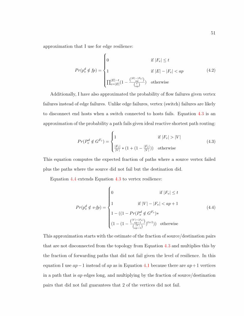
51
approximation that I use for edge resilience:
Pr(pdv /∈ fp) =
0 if |Fe| ≤ t
1 if |E| − |Fe| < ap∏|E|−te=|E|(1−
(|E|−|Fe|ap )
( eap)
) otherwise
(4.2)
Additionally, I have also approximated the probability of flow failures given vertex
failures instead of edge failures. Unlike edge failures, vertex (switch) failures are likely
to disconnect end hosts when a switch connected to hosts fails. Equation 4.3 is an
approximation of the probability a path fails given ideal reactive shortest path routing:
Pr(P dv /∈ GFv) =
1 if |Fv| > |V |
|Fv ||V | ∗ (1 + (1− |Fv |
|V | )) otherwise
(4.3)
This equation computes the expected fraction of paths where a source vertex failed
plus the paths where the source did not fail but the destination did.
Equation 4.4 extends Equation 4.3 to vertex resilience:
Pr(pdv /∈ v-fp) =
0 if |Fv| ≤ t
1 if |V | − |Fv| < ap + 1
1− ((1− Pr(P dv /∈ GFv)∗
(1− (1− (|V |−|Fv |ap−1 )
( |V |ap−1))t+1)) otherwise
(4.4)
This approximation starts with the estimate of the fraction of source/destination pairs
that are not disconnected from the topology from Equation 4.3 and multiplies this by
the fraction of forwarding paths that did not fail given the level of resilience. In this
equation I use ap−1 instead of ap as in Equation 4.1 because there are ap+1 vertices
in a path that is ap edges long, and multiplying by the fraction of source/destination
pairs that did not fail guarantees that 2 of the vertices did not fail.
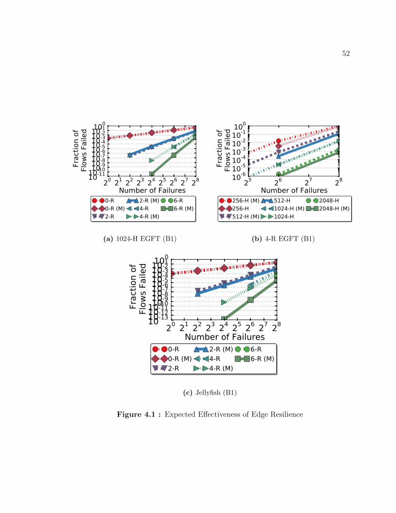
52
20 21 22 23 24 25 26 27 28
Number of Failures10-1110-1010-910-810-710-610-510-410-310-210-1100
Frac
tion
ofFl
ows
Faile
d
0-R0-R (M)2-R
2-R (M)4-R4-R (M)
6-R6-R (M)
(a) 1024-H EGFT (B1)
25 26 27 28
Number of Failures10-610-510-410-310-210-1100
Frac
tion
ofFl
ows
Faile
d
256-H (M)256-H512-H (M)
512-H1024-H (M)1024-H
2048-H2048-H (M)
(b) 4-R EGFT (B1)
20 21 22 23 24 25 26 27 28
Number of Failures10-1310-1210-1110-1010-910-810-710-610-510-410-310-210-1100
Frac
tion
ofFl
ows
Faile
d
0-R0-R (M)2-R
2-R (M)4-R4-R (M)
6-R6-R (M)
(c) Jellyfish (B1)
Figure 4.1 : Expected Effectiveness of Edge Resilience

53
In addition to quantifying the expected probability of routing failure, I would like
to verify the accuracy of Equation 4.2, Equation 4.3, and Equation 4.4. To do so, I
simulated different sizes and modes of routing failures according to the methodology
described in Section 4.7 given different levels of failure identifying resilience. Fig-
ure 4.1 presents the results of my experiments on full bisection (B1) fat trees, with
*-R and *-H representing differing levels of resilience and numbers of hosts, respec-
tively, and (M) marking the output of my approximation. Figure 4.1a not only shows
that my approximation is accurate across a range of levels of resilience on an EGFT
with 1024 hosts but also that linear increases in resilience provide orders of magnitude
decreases in the probability of routing failure.
To show the impact of topology size, Figure 4.1b presents the probability of routing
failure given a varying number of failures and 4-resilience on EGFT topologies. I chose
to use the same sizes of edge failures for each topology size instead of normalizing the
failure sizes to the topology because the most simultaneous link failures reported in
any of tens of production data centers was 180 [5]. Thus, the probability of failing
in Figure 4.1b decreases with topology size. The most notable aspect of this figure
is that, even though the forwarding tables only provide 4-resilience, the first failures
that I observed occurred only when 64 links were failed.
Although elided, I find that the probability of routing failure on Jellyfish topolo-
gies [47] is similar but slightly less than the results in Figure 4.1, and my approxi-
mation is similarly accurate. In the end, the accuracy of my approximation of the
probability of routing failure given edge resilience in my experiments was always
within an order of magnitude and frequently within a factor of 2–3×.
To show the accuracy of my approximations given vertex resilience, Figure 4.2
shows the approximated probability of failure and fraction of failed routes computed

54
20 21 22 23 24
Number of Failures10-3
10-2
10-1
100Fr
actio
n of
Flo
ws
Faile
d
0-R0-R (M)
2-R2-R (M)
SPSP (M)
(a) Failed Vertices
20 21 22 23 24 25 26
Number of Failures10-4
10-3
10-2
10-1
Frac
tion
of F
low
s Fa
iled
0-R 2-R
(b) Failed Edges
Figure 4.2 : Effectiveness of Vertex Resilience on a 4096 host EGFT Topology
from simulations for both edge and vertex failures given vertex resilience on the EGFT
topology. Because vertex failures can cause failures even in shortest path routing if
a vertex with hosts attached fails, I present the number of failures given reactive
shortest path routing in lines labeled SP, and, as before, the sets of edges and vertices
were selected randomly.
Figure 4.2 shows that my vertex failure approximation is accurate, and even mod-
erate levels of vertex resilience are effective at preventing avoidable routing failures.
However, vertex resilience does not provide significant protection given edges failures.
This is expected, because, if the last hop of a path fails, then vertex resilience assumes
that the switch failed.
On the other hand, edge resilience is also effective at preventing routing failures
given vertex failures. While not presented, the results for edge resilience look the same
as the results for vertex resilience in Figure 4.2a. This implies that edges resilience
is effective at mitigating both edge and vertex failures, but vertex resilience is only

55
10−1
Fraction of Flows Failed
0.0
0.2
0.4
0.6
0.8
1.0
Cum
mul
ativ
eFr
actio
n
C NC
(a) 0-R Routes
10−5 10−4 10−3
Fraction of Flows Failed
0.0
0.2
0.4
0.6
0.8
1.0
Cum
mul
ativ
eFr
actio
n
C NC
(b) 4-R Routes
Figure 4.3 : CDF of the fraction of failed routes given 64 edges failures on a 1024
host EGFT (B1)
effective given vertex failures. Combining this with a failure study of a production
datacenter network that claims that multiple switches failing at the same time is “ex-
tremely rare” [5], providing edge protection is more desirable than vertex protection.
Because of this, I only consider edge resilience for the rest of this thesis.
Correlated Failures
In practice, I would expect that simultaneous failures are likely to be physically
related. While failures that are due to manufacturing defects or hardware failure
would be expected to be independent, some failures, such as power outages or cutting
a bundle of cables, may affect a localized region of the topology. To evaluate this
case, I randomly selected sets of connected edges for failure (Section 4.7).
To illustrate the effect of correlated and non-correlated failures, Figure 4.3 shows a
CDF of the fraction of routes that failed with both 0-resilience (0-R) and 4-resilience
(4-R) given correlated (C) and non-correlated (NC) failures on a 1024 host EGFT
topology. Interestingly, correlated failures have less impact than non-correlated fail-

56
202122232425262728
Number of Failures
10−810−710−610−510−410−310−210−1
100Fr
actio
nof
Flow
sFa
iled
0-R2-R
4-R6-R
(a) EGFT (B1)
202122232425262728
Number of Failures
10−5
10−4
10−3
10−2
10−1
100
Frac
tion
ofFl
ows
Faile
d
0-R2-R
4-R6-R
SP
(b) EGFT (B6)
202122232425262728
Number of Failures
10−4
10−3
10−2
10−1
100
Frac
tion
ofFl
ows
Faile
d
0-R2-R
4-R6-R
(c) 99%tile EGFT (B1)
Figure 4.4 : Resilience and Correlated Failures
ures for the 0-R routes, although both still have a significant number of failed routes.
However, with 4-R routes, correlated failures cause more routes to fail than uniform
random failures. This is because 0-R routes fail if even a single edge on its path fails
and correlated failures are likely to touch fewer routes. 4-R routes, on the other hand,
only fail given multiple failures, so about 70% of all 64 edge failures do not even cause
a single routes to fail, while all correlated failures of 64 edges caused some routes to
fail, albeit at between two and four orders of magnitude fewer than without resilient
routes.
Figure 4.4 further illustrates this scenario by showing the average and 99th per-
centile fraction of routes that failed given correlated failures for varying levels of
resilience (*-R) on the 1024-host topologies, with B6 representing a 1 : 6 bisection
bandwidth ratio. Even though correlated failures impact roughly an order of mag-
nitude more routes, Figure 4.4a shows that the probability of failure is still low.
Although smaller topologies are more likely to be impacted by failures, Figure 4.4b
shows that resilience is still effective on the smaller B6 topology, and 6-resilience is

57
not all that far from reactive shortest path routing (SP). Lastly, Figure 4.4c, which
looks at the 99th percentile failures, shows that even though the outlying failures
impacted roughly an order of magnitude more routes than the average failures, low
levels of resilience still prevent far more routing failures than no resilience (0-R).
Given that I find low levels of resilience to be highly effective in preventing routing
failures, I am now primarily concerned with feasibly implementing resilience.
4.2 Definitions
In order to describe failure identifying and disjoint tree resilience, I, as before, use a
network model that is extended from that used by Feigenbaum et al. [30]. Formally,
a network is modeled as an undirected graph G = (V,E), where V = {1, . . . , n} and
{u, v} ∈ E. I define Ev = {{u, v} ∈ E;u, v ∈ V } as the set of edges local to vertex
v ∈ V . The powerset 2Ev is a bitmask representing the failure status of the edges in
Ev. E∗v is the set of all paths starting at v, and P d
v ⊆ E∗v is the set of all paths from
v to d. D is the set of destinations. Lastly, ATd is a set of arc-disjoint trees rooted
at node d, where an arc is one direction of a bi-directional edge, and ET is a set of
edge-disjoint trees.
In this model, each node v ∈ V has a forwarding function fv(d, ∗, bm) → p that
maps a packet’s destination d ∈ D and addition label as a function of a bitmask
bm ∈ 2Ev of the node’s state to a path p ∈ E∗v . For convenience, I also represent the
forwarding function as fv(d, ∗, Fv, e) → p, where Fv is a set of local edges that must
be failed and e is an edge that must be up, so as to compactly specify a bitmask over
the local incident edges.
While the rest of this chapter is concerned with resilient forwarding functions,
Table 4.1 presents a few non-resilient forwarding functions so as to both provide a

58
Network Architecture Forwarding Function Explanation
Non-Resilient
Traditional IP and Ethernet fi : D → Ei Pick a single output edge
per destination.
ECMP fi : D × 2Ei → Ei For each destination, pick
an output edge as a func-
tion of which incident
edges are up
Feigenbaum et al. [30] fi : D × Ei × 2Ei → Ei For each destination,
map incoming edges to
outgoing edges as a func-
tion of which incident
edges are up
Axon [48], SecondNet [49] fi : D → P di Pick a single forwarding
path per destination
Table 4.1 : Different non-resilient forwarding functions

59
point of comparison and help illustrate the formalism.
4.3 Failure Identifying (FI) Resilience
This section introduces failure identifying resilience (FI). First, this section starts of
by introducing the routing algorithm for FI resilience, and then this section discusses
three different FI resilient forwarding functions.
4.3.1 Forwarding Table Construction
Algorithm 1 – FI Routing for t-resilient forwarding
1. Build default (non-resilient) routes:
2. Iteratively protect routes against any single additional failure each round:
For round i in {1, . . . , t}, do:
(a) Consider every edge e and switch sw that forwards out e in all the paths p built in
round i− 1.
i. Build a backup path for p assuming that edge e failed, if one exists. This path must
not use either e or any edge that p assumes failed.
ii. Install a route at sw that uses p and modifies the packet to add e to the set of failures
identified by the packet.
To build t-resilient forwarding tables for failure identifying resilience, I use Algo-
rithm 1. This algorithm uses a very simple approach to route construction where the
actual path selection is left up to an arbitrary policy. Later, in Section 4.5.3, I show
that this flexibility can be used to implement compression-aware routing. At the
start, Algorithm 1 establishes all-to-all communication by installing a default route
for all source/destination pairs of hosts. Unless one of the edges in the path fails,

60
each switch along the route will use a packet’s header to look up an output port in
its forwarding table. The remainder of the routing algorithm iteratively increases
resilience by installing new backup routes to protect the paths built in the previous
round against the failure of any one additional edge. For every edge in the routes built
in the previous round, a backup route that matches the header of packets following
the route but requires the original output port to be down is added to the vertex
local to the edge. Because all possible failures of an additional edge are considered
in each round, by the end of round t, paths have been built that are resilient to all
possible failures of t edges. While the algorithm is presented in terms of edges, the
algorithm can also be used to protect against the failure of vertices, i.e. switches.
Figure 4.5 illustrates the routing algorithm by showing fully resilient routes for
II→Dst. In the figure, routes are represented as arrows and the level of resilience is
shown by the line style and color, using 0-R, 1-R, and 2-R for forwarding patterns that
are resilient to 0, 1, and 2 failures, respectively. Figure 4.5c is particularly interesting
because there are two 2-R entries. This is because failure information is only known
locally by the forwarding hardware, i.e., switches only learn of the failure of local
links, and the 1-R path [II-I, I-Dst ] can fail at either the II-I link or the I-Dst link
when there is still an operational path to Dst. Therefore, if links II-Dst and I-Dst
have failed, switch II will still attempt to forward packets along the [II-I, I-Dst ] path
based on its local information. Only after packets reach switch I will the failed link
I-Dst be observed, at which point the packet needs to be forwarded along the path
[I-II, II-III, III-Dst ]. While this leads to path stretch in this example, the stretch
tends to be minimal in practice and is unavoidable given that I want to provide local
fast failover without any a priori failure knowledge.
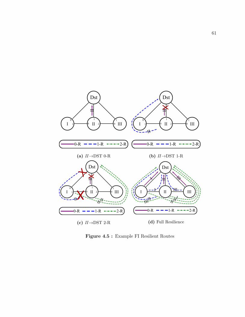
61
0
1
1
0 0
1
2I II III
II
0-R 1-R 2-R
Dst
(a) II→DST 0-R
0
1
1
0 0
1
2I II III
II
II
0-R 1-R 2-R
X
Dst
(b) II→DST 1-R
0
1
1
0 0
1
2I II III
II
II
IIII
0-R 1-R 2-R
XX
X
Dst
(c) II→DST 2-R (d) Full Resilience
Figure 4.5 : Example FI Resilient Routes

62
4.3.2 Forwarding Models
The principal difficulty in forwarding packets along the routes built by Algorithm 1
is in identifying which backup route a packet is currently following and what fail-
ures the packet has already encountered. In this thesis, I consider three forwarding
models with two features that are sufficient to support failure identifying resilience:
1) forwarding tables that not only match on packet headers, but also on the local
port status, and 2) packets with a header that identifies the set of failures already
encountered by the packet.
Although no datacenter switches currently implement the first feature in hardware,
the motivation for it is clear: matching on the current port status allows for near
instantaneous use of backup routes in the case of link failure. However, the reason
for the second feature may not be so clear. In particular, for some topologies and
levels of resilience, it is not necessary. Feigenbaum et al. [30] proved that it is always
possible to protect against any single link failure given a forwarding function that
only matches on the destination, the input port, and the current port status. Despite
this, all of the forwarding models I consider in this chapter utilize a packet header to
identify failures. In part, this is because I would like a forwarding function that can
protect against the failure of more than one link; Gill et al. found that only 59% of
failures involve a single edge [5]. If an additional header is not used to identify failures,
Theorem 2.3.1 also proves that there exists a topology for which there exists a level
of resilience that cannot be provided. The intuition behind this result is that, if a
packet encounters multiple failures, a switch cannot determine the exact set of failures
encountered by the packet, which can cause backup routes to form forwarding loops.
With an additional packet header, it becomes possible to build routes that protect

63
against any possible set of failures on any topology [25, 50]. Further, routes that use
an additional header are potentially less restricted than those that do not, potentially
leading to improved performance.
The first of these forwarding models, FCP, accumulates the IDs of the failed links
encountered by a packet in a header [25]. More precisely, FCP can either accumulate
edge IDs or use a label to identify a set of failed edges, which can save space.
With MPLS-FRR [26], I use a unique ID for every new route to provide t-resilience,
with the ID assigned to a packet changing when a failure is encountered. In fact, a
given network path may have multiple IDs, because an ID also encodes the route
that was being used by the packet prior to each encountered failure. Thus, the set of
encountered failed edges can be inferred from the ID.
Plinko, the final forwarding model that I consider, is a new model that retains the
full path taken by a packet to identify the set of failures encountered by that packet.
The failures can be identified because the retained path includes the packet’s source
at each hop, and, from a given source–be it the original switch or the switch local
to a failure–there is only one possible path forward given the local failures. This is
due to the resilient routing algorithm, which causes all forwarding table entries for a
packet (reverse path) at a switch to use different paths and protect against a different
set of failures. This implies that the path a packet has taken can be used to infer the
original source, the forwarding table entries used to forward the packet, and thus the
exact set of failures the packet has encountered. (A more detailed proof that Plinko
is t-resilient can be found in a tech report [51].)
In Plinko, the full path taken by a packet is retained by having every switch that
the packet traverses push the packet’s input port number onto a list contained in
the packet header. In effect, this simple action creates a list of ports that identify a

64
Network Architecture Forwarding Function Explanation
Exhaustive Resilient
Plinko fi : D × E∗i × 2Ei → {Ei, Pdi } For each destination,
map the reverse path
to an outgoing edge or
forwarding path as a
function of which inci-
dent edges are up
MPLS-FRR [26] fi : D × P d × 2Ei → {Ei, Pdi } For each destination,
map the current path
ID to an outgoing edge
or forwarding path as
a function of which in-
cident edges are up
FCP [25] fi : D × 2E × 2Ei → {Ei, Pdi } For each destination,
map the set of failed
edges already encoun-
tered by a packet to an
outgoing edge or for-
warding path as a func-
tion of which incident
edges are up
Table 4.2 : Different FI resilient forwarding functions
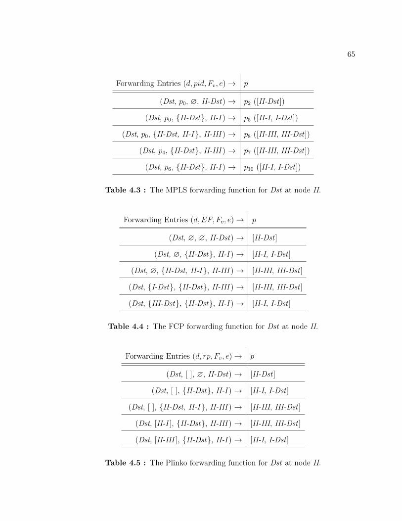
65
Forwarding Entries (d, pid, Fv, e)→ p
(Dst, p0, ∅, II-Dst) → p2 ([II-Dst ])
(Dst, p0, {II-Dst}, II-I ) → p5 ([II-I, I-Dst ])
(Dst, p0, {II-Dst, II-I }, II-III ) → p8 ([II-III, III-Dst ])
(Dst, p4, {II-Dst}, II-III ) → p7 ([II-III, III-Dst ])
(Dst, p6, {II-Dst}, II-I ) → p10 ([II-I, I-Dst ])
Table 4.3 : The MPLS forwarding function for Dst at node II.
Forwarding Entries (d,EF, Fv, e)→ p
(Dst, ∅, ∅, II-Dst) → [II-Dst ]
(Dst, ∅, {II-Dst}, II-I ) → [II-I, I-Dst ]
(Dst, ∅, {II-Dst, II-I }, II-III ) → [II-III, III-Dst ]
(Dst, {I-Dst}, {II-Dst}, II-III ) → [II-III, III-Dst ]
(Dst, {III-Dst}, {II-Dst}, II-I ) → [II-I, I-Dst ]
Table 4.4 : The FCP forwarding function for Dst at node II.
Forwarding Entries (d, rp, Fv, e)→ p
(Dst, [ ], ∅, II-Dst) → [II-Dst ]
(Dst, [ ], {II-Dst}, II-I ) → [II-I, I-Dst ]
(Dst, [ ], {II-Dst, II-I }, II-III ) → [II-III, III-Dst ]
(Dst, [II-I ], {II-Dst}, II-III ) → [II-III, III-Dst ]
(Dst, [II-III ], {II-Dst}, II-I ) → [II-I, I-Dst ]
Table 4.5 : The Plinko forwarding function for Dst at node II.

66
path from the current switch back to the source of the packet, i.e., the reverse of the
path taken by the packet. The primary benefits of Plinko are that the same action
is applied to every packet and that packets with common reverse path prefixes may
have encountered the same failures and have the same output path, which allows for
rules to be compressed.
Lastly, I consider versions of all three forwarding models where the output of the
forwarding function is a single edge, which leads to hop-by-hop forwarding, and where
the output of the forwarding function is a full source-route that is added to the packet
in addition to the tags used for resilient forwarding. While this distinction does not
affect resilience, source-routing can require less state.
To formalize the MPS-FRR, FCP, and Plinko forwarding models, Table 4.5 for-
mally specifies the different FI resilient forwarding functions. To provide a concrete
example for all three forwarding models, Table 4.5, Table 4.3, and Table 4.4 show the
forwarding function for node II in Figure 4.5 given MPLS-FRR, FCP, and Plinko,
respectively. Although the forwarding function entries are symbolic, it is also possible
to represent each entry as an opaque blob of bits suitable for matching in hardware.
4.4 Disjoint Tree Resilience
While FI resilience protects against the failure of specific sets of edges or vertices for
a given path, disjoint tree resilience builds disjoint spanning trees that are used to
protect against failures. In this thesis, I consider both EDST resilience, which builds
edge-disjoint spanning trees, and ADST resilience, which builds arc-disjoint spanning
trees.
In both of these forwarding models, when a failure is encountered, the current tree
is marked as failed and a new tree is selected for forwarding. In effect, the failure of

67
an edge or arc is treated as the failure of the tree that the edge or arc belongs to.
This failure is then marked in a packet header, and forwarding continues until either
the destination is reached or there are no more trees left.
In contrast with FI resilience, the addition of another disjoint tree protects a given
destination against a single additional failure for all possible sources, while each set of
failures must be considered independently in FI resilience, possibly for each source and
destination pair. On the other hand, the FCP, MPLS-FRR, and Plinko forwarding
functions are capable of t-resilient routing for all values of t, while ADST and EDST
resilience can only protect against k−1 and k/2−1 failures on a k connected topology,
respectively [29].
To be more formal, the Table 4.6 shows the forwarding functions for ADST and
EDST resilience. Although it is crucial in disjoint tree resilience to continue forward-
ing on the current tree until it fails, it may appear odd that the forwarding functions
for ADST and EDST do not match on a packet header than contains the current tree
ID. This is because the input port of a packet can be used to identify the current tree
due to the fact that ADST and EDST use disjoint trees. However, I also consider
variants of both ADST and EDST resilience that also mark the current tree in a
packet header, which can reduce forwarding table state because a switch is likely to
have more than one incident input edge for a given tree.
As with FI resilience, disjoint tree resilience needs a specific routing algorithm.
Routing for EDST tree resilience is conceptually simple. All routes follow the paths
defined by a tree until a failure is encountered, and then any non-failed tree may
be selected for forwarding. On the other hand, ADST tree resilience imposes more
restrictions on routing. This is because the failure of a single edge causes the failure of
two arcs. Specifically, each edge can be traversed in two directions, which are referred

68
Network Architecture Forwarding Function Explanation
Disjoint Tree Resilient
ADST [29] fi : D × Ei × 2ATd × 2Ei → Ei For each destination,
pick an outgoing edge
as a product of the in-
put port, which iden-
tifies a tree, a bitmask
of already failed arc-
disjoint trees, and the
current port status
EDST [29] fi : D × Ei × 2ET × 2Ei → Ei For each destination,
pick an outgoing edge
as a product of the in-
put port, which identi-
fies a Tree, a bitmask
of already failed edge-
disjoint trees, and the
current port status
Table 4.6 : The different disjoint tree resilient hardware forwarding functions

69
to as arcs, and if an edge fails, it cannot be traversed in either direction. Therefore,
the important property necessary for routing with (t + 1) ADSTs to be t-resilient is
that each failed edge is only visited once. To insure this property, after an edge has
failed, the next ADST that is chosen must be the ADST that a packet that enters
the switch on the failed edge would use, if one exists, and this thesis refers to such
an ADST as a reverse tree. Given this restriction, the packet will either reach the
destination on the reverse tree or it will encounter a failure. Either way, the packet
is guaranteed to never traverse the same failed edge twice.
However, the routing algorithms described for EDST and ADST by prior work [29]
are best suited as on-line software algorithms because packets are modified and then
reprocessed, potentially multiple times. While this works well in software, in hardware
this would require packets be resubmitted through the packet processing pipeline,
which would increase the maximum number of packets per second that a switch must
process, potentially overloading the switch during failures. To solve this problem, this
thesis introduces new routing algorithms for EDST and ADST that are better suited
for hardware.
Algorithm 2 and Algorithm 3 are the new routing algorithms for the EDST and
ADST forwarding functions, respectively. Unlike the software routing algortihms,
the core idea behind these algorithms is to install forwarding entries for all possible
combinations of destinations, input ports, failed tree identifiers, and failed local ports.
This enables correct fault-tolerant routing to be performed in a single pass through
the matching hardware.
One thing that may seem odd about the EDST and ADST routing algorithms is
that the forwarding function specifies a bitmask as a combination of a tree or port
that must be up and a set of trees or edges that must be failed, yet all of the sets of

70
Algorithm 2 – EDST RoutingInput: network topology G = (V,E) where V = {1, . . . , n}, and a set of edge-disjoint trees
ET .
Output: a forwarding pattern f = (f1, . . . , fn). ∀v ∈ V , fv(d, ip, t, FT , e, Fv) → (e, FET ),
where d ∈ D is the destination, ip ∈ Ev is the input port, t ∈ ET is a tree label that
must not be failed, FT ⊆ ET is a set of trees that must be marked as failed, e ∈ Ev is
an edge that must not be failed that is also used as the output edge, Fv ⊆ EV is a set
of edges that must be failed, and FET ⊆ ET is a set of trees to mark as failed in the
packet’s header.
1. Build non-failure routes at each vertex for each destination for each input
port tree: ∀v ∈ V , ∀d ∈ D, and ∀ip ∈ Ev, do:
• Let t ∈ ET be the tree that ip is a member of, i.e., ip ∈ t. If t does not exist, continue.
• Let e ∈ t be the output edge on t’s route to d.
• Set fv(d, ip, t,∅, e,∅) := (e,∅)
2. Build failure routes at each vertex for each destination for each input port
tree: ∀v ∈ V , ∀d ∈ D, and ∀ip ∈ Ev, do:
• Let t ∈ ET be the tree that ip is a member of, i.e., ip ∈ t. If t does not exist, continue.
• Let FET := {t} be the set of trees to mark as failed.
• For each alternate tree: ∀at ∈ ET − {t}
– Let e ∈ t be the output edge on at’s route to d.
– Set fv(d, ip, at,∅, e,∅) := (e, FET )
– Let FET := FET ∪ {at}

71
Algorithm 3 – ADST RoutingInput: network topology G = (V,E) and a set of arc-disjoint trees AT .
Output: a forwarding pattern f = (f1, . . . , fn). ∀v ∈ V , fv(d, ip, t, FT , e, Fv) → (e, FATd),
where d ∈ D is the destination, ip ∈ Ev is the input port, t ∈ ATd is a tree label that
must not be failed, FT ⊆ ATd is a set of trees that must be marked as failed, e ∈ Ev is
an edge that must not be failed that is also used as the output edge, Fv ⊆ EV is a set
of edges that must be failed, and FATd⊆ ATd is a set of trees to mark as failed in the
packet’s header.
1. Build non-failure routes at each vertex for each destination for each input
port tree: ∀v ∈ V , ∀d ∈ D, and ∀ip ∈ Ev, do:
• Let t ∈ ATd be the tree that ip is a member of, i.e., ip ∈ t. If t does not exist, continue.
• Let e ∈ t be the output edge on t’s route to d.
• Set fv(d, ip, t,∅, e,∅) := (e,∅)
2. Build failure routes at each vertex for each destination for each input port
tree: ∀v ∈ V , ∀d ∈ D, and ∀ip ∈ Ev, do:
• Let t ∈ ATd be the tree that ip is a member of, i.e., ip ∈ t. If t does not exist, continue.
• Let FATd:= {t} be the set of trees to mark as failed.
• Let NATd:= ATd − {t} be the set of alternate trees to use if t fails
• While there exist alternate trees: While |NATd| > 0
– Let at ∈ NATdbe an alternate tree.
– Let e ∈ at be the output edge on at’s route to d.
– Set fv(d, ip, at,∅, e,∅) := (e, FATd)
– Remove at from the alternate trees. Let NATd:= NATd
− {at}
– Add at to the failed trees. Let FATd:= FATd
∪ {at}
– Reverse Tree Forwarding: If e is an input port for any tree rat ∈ NATd:
∗ Let re ∈ rat be the output edge on rat’s route to d.
∗ Set fv(d, e, rat,∅, re,∅) := (re, FATd)
∗ Remove rat from the alternate trees. Let NATd:= NATd
− {rat}
∗ Add rat to the failed trees. Let FATd:= FATd
∪ {rat}

72
trees and ports necessary to be down are null sets. This is because the rules need to
cover all possible cases of packets, including those that have seen no failed trees, and
those that have seen all but one tree marked as failed. Similarly, it is possible for any
switch to see the failures of all of the possible spanning trees due to just local link
failures. Thus, the reason that the null failed sets are explicitly part of the forwarding
function is because all possible permutations of failed trees and edges must be able
to be forwarded.
Further, when converted to bitmasks, these algorithms install overlapping rules in
the forwarding function. These algorithms operate under the assumption that earlier
entries are not overwritten by subsequent entries. In effect, this means that earlier
entries have a higher priority than later entries, which, in the context of the algorithm,
means that the forwarding function specifies an order in which to try alternate trees
in the event of a failure.
When the next forwarding tree is not specified by the routing algorithm, as it may
sometimes be in ADST resilience, the next forwarding tree in the case of a failure
may be any non-failed tree. Because the choice of tree does not impact resilience, I
use a shortest-tree first routing policy in the interest of performance.
As a performance optimization, multiple shortest path trees can be also built for a
given destination in addition to the disjoint spanning trees that are build for resilience
in both ADST and EDST. Although the shortest path trees do not necessarily provide
additional resilience and packets would need to carry a current tree label if the shortest
path trees are not disjoint from the resilient trees, they are useful because they can
be used to implement random shortest path first routing. In this case, disjoint tree
resilient should only incur stretch and impact performance only when there are failures
in the network.

73
I II III
1-T 2-T
Dst
Figure 4.6 : EDST resilient routes for Dst
Forwarding Entries (d, ip, t, FT , e, Fv)→ (e, FET
(Dst, self, 1-T, ∅, II-Dst, ∅) → ([II-Dst ], ∅)
(Dst, self, 2-T, ∅, II-I, ∅) → ([II-Dst ], {1-T})
(Dst, III-II, 2-T, ∅, II-I, ∅) → ([II-I ], ∅)
(Dst, III-II, 1-T, ∅, II-Dst, ∅) → ([II-Dst ], {2-T})
Table 4.7 : The EDST forwarding function for Dst at node II in Figure 4.6.

74
I II III
SP 1-T 2-T
Dst
Figure 4.7 : ADST resilient routes for Dst
To illustrate the EDST routing algorithm, Figure 4.6 shows a topology and two
edge-disjoint spanning trees, and Table 4.7 shows the forwarding function of node II
in Figure 4.6 if Algorithm 2 was used for routing. In the topology shown in Figure 4.6,
the nodes are the sources of traffic, so traffic originating at a given node are marked
as coming from the self input port in Table 4.7. In practice, most traffic originates
from hosts, which have their own input ports, and traffic that does originate from the
switch control plane also has it’s own input port.
Similar to Figure 4.6, Figure 4.7 shows a topology and two arc-disjoint spanning
trees, and Table 4.8 shows the forwarding function of node II in Figure 4.7 if Algo-
rithm 3 was used for routing. As before, packets that originate at a switch are marked
as coming from the self input port. Also, because there are only two possible arc-
disjoint spanning trees given the topology in Figure 4.7, the reverse tree forwarding
required in ADST resilience is also the only possible alternate tree.
Figure 4.7 includes an extension to ADST resilience not included in Algorithm 3.
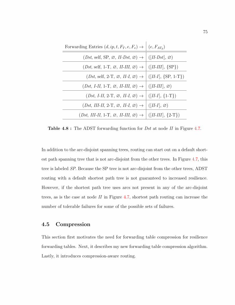
75
Forwarding Entries (d, ip, t, FT , e, Fv)→ (e, FATd)
(Dst, self, SP, ∅, II-Dst, ∅) → ([II-Dst ], ∅)
(Dst, self, 1-T, ∅, II-III, ∅) → ([II-III ], {SP})
(Dst, self, 2-T, ∅, II-I, ∅) → ([II-I ], {SP, 1-T})
(Dst, I-II, 1-T, ∅, II-III, ∅) → ([II-III ], ∅)
(Dst, I-II, 2-T, ∅, II-I, ∅) → ([II-I ], {1-T})
(Dst, III-II, 2-T, ∅, II-I, ∅) → ([II-I ], ∅)
(Dst, III-II, 1-T, ∅, II-III, ∅) → ([II-III ], {2-T})
Table 4.8 : The ADST forwarding function for Dst at node II in Figure 4.7.
In addition to the arc-disjoint spanning trees, routing can start out on a default short-
est path spanning tree that is not arc-disjoint from the other trees. In Figure 4.7, this
tree is labeled SP. Because the SP tree is not arc-disjoint from the other trees, ADST
routing with a default shortest path tree is not guaranteed to increased resilience.
However, if the shortest path tree uses arcs not present in any of the arc-disjoint
trees, as is the case at node II in Figure 4.7, shortest path routing can increase the
number of tolerable failures for some of the possible sets of failures.
4.5 Compression
This section first motivates the need for forwarding table compression for resilience
forwarding tables. Next, it describes my new forwarding table compression algorithm.
Lastly, it introduces compression-aware routing.

76
10GbE Switch Release Year TCAM Exact Match
HP Procurve 5400zl 2006 285 Kbit 918 Kbit
Intel FlexPipe (FM6000)? 2011 885 Kbit 5 Mbit
BNT G8264 2011 ∼1.15 Mbit ∼5.6 Mbit
Metamorphosis? 2013 † 40 Mbit 370 Mbit
Table 4.9 : 10 Gbps TOR Switch Table Sizes. A ? indicates that the switch is
reconfigurable, and a † indicates that the switch is academic work and not a full
product.
4.5.1 Motivation
Because both FI and disjoint tree resilient forwarding install more forwarding table
entries than non-resilient forwarding would, it is desirable to try to compress resilient
forwarding tables so as to reduce some of the impact of fault tolerant forwarding.
However, disjoint tree resilience, unlike FI resilience, uses a routing algorithm that
installs overlapping entries where the order of the entries is important for perfor-
mance. In order to compress these forwarding tables, the entries would need to be
reordered, which could hurt performance. Further, state in disjoint tree resilience is
only proportional to the number of trees squared, which implies there is little need to
compress disjoint tree resilient forwarding tables. Because of this, I do not consider
compressing disjoint tree resilience.
On the other hand, FI resilience builds forwarding tables with non-overlapping
entries and the number of forwarding table entries is roughly exponential with respect
to the level of resilience, so compressing forwarding tables will not impact performance

77
28 29 210 211 212
Number of Hosts
102
103
104TC
AM S
ize
(Kb)
PlinkoMPLS-FRR
FCPMPLS-FRR (Lower Bound)
FCP (Lower Bound)Compressed Plinko
Figure 4.8 : TCAM Sizes for 6-Resilience
and may be necessary to implement FI resilience on realistic topology sizes. Thus, this
section focuses specifically on compressing FI resilient forwarding tables, exploring the
validity of the assumption made in prior work that the state explosion in FI resilience
would limit hardware it to all but the smallest networks or uninteresting levels of
resilience [25]
To that end, I built 6-resilient FI routes between all host-pairs in a network for a
range of different sized full bisection bandwidth fat tree topologies to understand the
exact state requirements of resilience (see Section 4.7 for the details of my methodol-
ogy). To see if the state requirements are prohibitive, I compare the results against
the TCAM sizes found in existing and proposed datacenter switches, which I present
in Table 4.9. The results of this experiment, shown in Figure 4.8, confirm the as-
sumptions of previous work. Providing 6-resilience requires over 40 Mbit of TCAM
state on a network with just two thousand hosts, more state than is available in any
switch, so this result clearly motivates forwarding table compression.
However, as was previously mentioned, modifying packets in transit is necessary

78
for t-resilience. Unfortunately, only forwarding table rules that share the same output
and packet modification action can be compressed, which is problematic for FCP
and MPLS-FRR. To illustrate this, Figure 4.8 shows the total state required for
only the modifying entries after applying network virtualization to also reduce state
(Section 4.6) in the “(Lower Bound)” lines in the figure.
As Figure 4.8 illustrates, tagging packets to identify the set of failures they have
already encountered in MPLS-FRR and FCP can lead to a large number of unique
packet modification actions. For example, when moving from (t − 1) to t-resilience
in MPLS-FRR, roughly |D|2 ∗ apt/|V | of the |D|2 ∗ ap(t+1)/|V | total extra forwarding
table entries added to each switch modify a header field to a unique tag, i.e. one for
every link in all of the (t−1) resilient routes, and these entries cannot be compressed.
Also, although FCP tags packets differently than MPLS-FRR, the compressibility of
FCP is similarly limited.
On the other hand, Plinko applies the same modification to each packet—pushing
the input port onto a list in the packet—so there is no such limitation. Surprisingly,
this subtle architectural difference is crucial to enabling forwarding table compression.
With all optimizations combined, I frequently saw a reduction in state of over 95%,
which is shown in Figure 4.8 as the line “Compressed Plinko.”
Although MPLS-FRR uses unique IDs for each route, it may seem reasonable to
try to adapt FCP so that it applies the same action to each packet. One way to do
this would be to have a switch mark a packet with all local failures instead of just
the failures specific to forwarding the packet, i.e., the specific set of local failures
the forwarding table entry protects against. However, this causes a few problems.
First, t-resilient routes must now be built to match on any of many possible different
failures marked in a packet’s headers by the switches the packet traverses, causing

79
an explosion in the number of entries. While it is then reasonable to try to compress
these entries, allowing for each switch to independently mark the failures of all of its
edges leads to prohibitively large packet headers.
4.5.2 Forwarding Table Compression
TCAMs can be used to reduce forwarding table state. As long as two forwarding table
entries have the same output and packet modification operations, wildcard matching
can be used to combine multiple forwarding table entries into a single TCAM entry by
masking off the bits in which the entries differ. Such forwarding table compression is
particularly powerful because TCAMs allow for overlapping entries, with the priority
of an entry determining which entry actually matches a packet. This introduces
an optimization problem: given a set of non-overlapping forwarding table entries,
find a smaller set of potentially overlapping TCAM entries and priorities that are
functionally equivalent. If the state reduction from compressing a resilient forwarding
table is greater than the increase in TCAM state from matching on the resilient tag
(or reverse path), then it is better to perform matching with a TCAM.
My work is not the first to discuss this use of TCAMs, and this optimization
problem has been well studied in the context of packet classifiers. However, most
of the existing work is not applicable to resilient forwarding, because it is designed
for prefix classifiers [52], whereas the port bitmask in resilient forwarding is not a
prefix rule. Simiarly, XPath [53] requires being able to assign labels to each path,
which does not fit with matching on a path in Plinko because assigning a label
to each route simply devolves into MPLS-FRR if applied to Plinko. To the best
of my knowledge, Bit weaving [52] is the only compression algorithm applicable to
Plinko. Unfortunately, it did not result in significant compression when applied to

80
resilient forwarding tables, most likely because Bit weaving was designed for packet
classifiers, whose table entries are different than those for resilience. Thus, I developed
a new TCAM packing heuristic, which performs well in my experiments. While
other effective compression algorithms potentially exist, their existence would only
complement and strengthen my arguments.
Specifically, my new TCAM packing heuristic is based on two observations. First,
higher priority entries in a TCAM have to be finer in granularity so as to avoid
matching packets intended for a lower priority entry. Second, there is a greater
chance for state reduction by choosing to aggregate the largest set of rules that share
a common output path first. Based on these observations, the algorithm first sorts
the rules in descending order based on the size of the set of rules that share the same
output path and action. In other words, for each (output, action) pair in the old table,
the algorithm builds the set of entries that use the pair then considers each entry in
each set, starting with the largest set. Because the earlier an entry is considered
for compression the more likely it is to be compressed in my algorithm, this order
ensures that the entries with a larger potential for reducing forwarding table size are
considered first.
Given this processing order, my algorithm then greedily attempts to merge entries,
i.e. masking off the bits in which they differ, into rules in a new TCAM, which I
initialize as empty. To do so, I maintain a working set of new TCAM entries for each
(output, action) pair, which I also initialize as empty. For each old entry in order,
the working set is greedily searched for a new entry to merge with the old entry such
that the resulting merged entry does not overlap with any committed TCAM entry.
In other words, if any of the already considered forwarding table entries with different
(output, action) pairs would match the new entry, then the merge is not performed,

81
but, if there is no conflict, then the merge is performed, updating the entry in the
working set. However, if all entries in the working set cause conflicts, then the current
old entry is added as-is to the working set. Lastly, once all entries for an (output,
action) pair are considered, the entries in the working set are committed to the new
TCAM at a priority higher than that of any entry currently committed to the new
TCAM.
4.5.3 Compression-Aware Routing
Forwarding table compression will always be constrained by the number of unique
output paths in the forwarding table. However, my resilient routing algorithm allows
for arbitrary paths, and, on datacenter topologies, the algorithm frequently chooses
between multiple equivalent paths. To exploit this property to improve compress-
ibility, I propose compression-aware routing, which attempts to choose routes that
increase the compressibility of the forwarding tables.
The compression-aware routing heuristic first checks if any of the existing routes
for the current destination avoid the failures that the current route being built protects
against. If so, the most common of such paths is chosen. If no such path exists, non-
compression-aware routing continues and chooses a new path that avoids the necessary
failures.
Because each backup route depends on the paths used by previous routes, the
order in which the routes are chosen can have an impact on compression. There
are two reasonable orderings, which are akin to BFS and DFS graph traversal: the
BFS ordering builds all possible t-resilient routes before building any (t+ 1)-resilient
routes, while the DFS ordering recursively protects the first unprotected hop of the
most recent route until the desired level of resilience is achieved.

82
I chose to use the BFS ordering for two reasons. First, lower-level resilient routes
are more important for performance. Given, t failures, there are likely to be more
routes that hit i < t failures than those that hit exactly t failures. Further, the
0-resilient routes are especially important to network performance because these are
the default routes. Second, there are likely to be more (t + 1)-resilient routes than
there are t-resilient routes, so considering them later may open up more opportunities
for reusing existing routes.
4.6 Implementation
In this section, I discuss how to implement the MPLS-FRR, FCP, Plinko, EDST,
and ADST forwarding functions given a reconfigurable (RMT) switch, such as either
Metamorphosis [31] or FlexPipe [43]. I take care to note how to implement the
forwarding functions while maintaining end-host transparency, which is necessary for
general applicability. Next, I discuss the implementation of source routing, which, in
addition to reducing forwarding table state, is necessary to retain the full path taken
by a packet in Plinko. After that, I also discuss network virtualization, a network
feature that, as a side effect, reduces forwarding state [54]. Lastly, I discuss how
to safely implement network updates. To the best of my knowledge, this section is
the first description of a method for implementing arbitrary fast failover groups for
Ethernet networks in hardware.
4.6.1 Resilient Logical Forwarding Pipeline
Recent developments have led to switches with both reconfigurable packet parsers and
reconfigurable match tables that support a multitude of generic packet matching and
modification actions (RMT [31] and FlexPipe [43]). Given reconfigurable switches,

83
Table Input Fields Match
Ac-
tions
Modified
Fields
Explanation
Island In
Table
InPort Drop ∅ Distinguish between packets based on
whether the input port is internal or not
Security
Table
* Drop Security Tag Perform arbitrary packet matching to
either drop packets or add a security tag
Encap/
MPath
Table
Dst ∅ VDst, ECMP
ID, ResTag,
RevHop-
Count
RevHops
Add the necessary default packet
headers to external packets. Optionally
converts overlay/end-host addresses into
underlay addresses, selecting among
multiple possible paths if applicable
SrcFwd/
Local
Table
((Dst × VDst) |
FwdHop[0]) ×
bm
OutPort FwdHopCount,
FwdHops
Source routing: checks to see if the
current next hop is operational. If not,
discard the forward source route
Network Virtualization: Checks to see if
the virtual destination is local and the
port of the physical destination is up
ResFwd
Table
(VDst | Dst) ×
(RevHops |
ResTag) × bm
× SecTag
OutPort,
Drop
FwdHopCount,
FwdHops,
ResTag
Choose an output edge or path as a
function of the destination, the
resilience tag or reverse path, and the
port status bitmask
SrcUpdate
Table
∅ ∅ Fwd/Rev
Source Route
Pop off the current FwdHop and Push
on the new RevHop
Island
Out
Table
OutPort ∅ Entire new
header
Decapsulate packets that leave the
island
Table 4.10 : Description of the tables in Figure 4.10.

84
Fwd Hop Count Fwd Hops Rev Hop Count Rev Hops Version Dst MPath ID Res Tag Sec Tag Eth Frame CRC
Source Routing !Plinko Routing Virt FCP and MPLS-FRR
Figure 4.9 : A Packet Header for Resilient Forwarding
Mandatory Optional
Island In Table
SrcFwd/LocalTable
ResFwd Table
SrcUpdateTable
Island OutTable
SecurityTable
Encap/MPathTable
Figure 4.10 : A Example Resilient Forwarding Pipeline
implementing our forwarding models should be simple. However, these models are
not limited to reconfigurable switches and could also be implemented on an FPGA
or ASIC.
Although, implementing local fast failover at the hardware level requires a for-
warding table that can match on the current port status of the local switch, I am not
aware of a switch that currently allows for matching on the port status as a p-bit value,
given a p-port switch. However, I believe that this change is easily implementable.
In particular, this port bitfield would be maintained based on PHY information and
used as an input to the forwarding table pipeline, where it is then best suited for
matching with a TCAM.
While matching on the current port status could also use exact match memory,
doing so would cause a prohibitive explosion in state. Most forwarding table entries

85
protect against a handful of failures and do so regardless of the state of the other
ports on the switch. If a single 1-resilient backup route is built that requires one edge
to be up and one to be down on a 64-port switch, ignoring the other 62 ports, using
a bitmask with wildcards can specify this match in a single TCAM entry, while using
exact match would require 262 separate entries to cover all possibilities.
Given a port bitmask for matching, it is simple to implement resilient FCP and
MPLS-FRR. In its basic form, the switch pipeline would consists of a single table
that uses exact match memory to match on the destination and resilience tag and a
TCAM for matching on the port bitfield. Each entry would then specify an output
port and, if a failure was encountered, write the new resilience tag to the packet.
Matching on the ADST and EDST forwarding functions is similar to matching
on the FCP and MPLS-FRR forwarding functions. However, the ADST and EDST
forwarding functions match on two different bitmasks: the current status of the local
ports and the status of the failed trees encountered by the packet. As with FCP and
MPLS-FRR, exact match memory is not well suited for matching on either bitmask.
Thus, both bitmasks require a TCAM for matching both the port and tree status
bitmasks used in ADST and EDST.
The rest of this section focuses on additional features for implementing Plinko
and reducing forwarding table state. While these features incur a slight bandwidth
overhead due to increased packet header overhead, the added benefit outweighs the
cost. To be concrete, Figure 4.9 presents an example packet header for resilient
forwarding. Further, Figure 4.10 presents an example resilient packet processing
pipeline, and Table 4.10 describes the functionality of each table in the pipeline,
referencing fields in the packet header, a packet’s input port InPort, its output port
OutPort, and the port bitmask of the switch bm. Together, Figure 4.10 and Table 4.10

86
are similar to P4’s Table Dependency Graphs (TDGs) [55].
While I think that these are a reasonable point in the design space, other variants
assuredly exist. For example, it may also be desirable to add length and type fields
to the packet header to simplify packet processing for networking monitoring tools
and to allow for dynamically switching between packet formats without interrupting
forwarding, respectively. Further, the header includes a version field that, while not
strictly necessary, is important for enabling simple, consistent network updates [56].
However, I believe that my example forwarding pipeline and packet header illustrate
the differences between key points in the design space, regardless of alternate imple-
mentations.
4.6.2 Source Routing
Source routing, where packets contain a full path in a header, can reduce forwarding
table state in FI resilience. In disjoint tree resilience, every switch must contain
routes for every destination on every tree, which is then guaranteed to provide all-to-
all routes because the trees are spanning trees. Because of this, the output at a switch
for a given tree can just be a single edge as every switch must have a rule for this tree.
However, in FI resilience, routes are installed for every individual source/destination
pair. If the path chosen for a given (backup) route for a source/destination pair is
more than one edge long, then forwarding table entries need to be installed on multiple
switches for this route in FI resilience if the output of the forwarding function is just
an output edge. If source routing is used, then only one forwarding table entry is
needed per route. This reduces forwarding table state in proportion to the average
path length of the network topology because forwarding table state is no longer stored
at the intermediate switches along a packet’s path.
87
However, this reduction in forwarding table state comes at the cost of increased
packet header overhead. To reduce this overhead, I reuse an existing architecture
for source-routed Ethernet that typically incurs an overhead of less than 1–2% [48].
While some other implementations of source routing use global switch or link ids to
describe routes, Axons significantly reduce packet header overhead on large networks
by labeling each next hop with a label that is local to the switch that forwards along
the hop. In effect, an Axon source route is a list of switch port numbers, one for
each switch along the path. Thus, an Axon source route is only meaningful given a
starting switch for the route. Further, Axons accumulate a reverse route in a packet
header as forwarding occurs, i.e., a list of port numbers that, when followed from
the current switch, lead back to the source of the packet. Because Plinko matches
on the reverse path of a packet to provide resilience, Plinko benefits from the Axon’s
compact source route not just from reduced packet header overhead but also from
reduced forwarding table state.
Although Axons were originally implemented in an FPGA, implementing the Axon
protocol with a reconfigurable switch is possible by using two small additional logical
tables, which are labeled as the SrcFwd and SrcUpdate tables in Figure 4.10. These
tables attempt to forward via the source route and update the source route, respec-
tively. The SrcFwd table matches on the next forward hop in the source route and
the current port status. This table is small, containing just one entry per switch port.
Each entry simply checks to see if the output port specified by the source route is
operational. If it is, then it is used. Otherwise, the forward source route is discarded,
and packet matching continues in the resilient forwarding table to find an alternate
route. The SrcUpdate table is even simpler as it applies the same increment, decre-
ment, push, and pop operations required to modify the forward and reverse source

88
routes to all packets.
Given transparent source routing, the principal difficulty in implementing a Plinko
switch is then in efficiently implementing the Plinko forwarding function. As with
FCP and MPLS-FRR forwarding functions, Plinko’s destination and label, which
is a reverse path, could be implemented with exact match tables. However, table
state is a limiting factor on scalability, and forwarding entries with reverse paths
with overlapping prefixes and the same output path can be compressed into a single
TCAM entry. If the state reduction from compression is greater than increase in
TCAM state from matching on the reverse path, then it is better to match on the
reverse path with a TCAM, which, in practice, is the case.
4.6.3 Network Virtualization
Network virtualization can also be used to reduce state [54]. Most hosts are only
attached to one or two switches, while top-of-rack (TOR) switches connect to many
hosts and many switches. This leads to the switch level topology being smaller than
the host level topology. However, using multiple paths is especially important when
forwarding on the switch topology so as to prevent all hosts on a switch from using
the same path. Thus, encapsulating packets from (virtual) end-hosts and routing on
the switch topology reduces state proportional to the number of (virtual) hosts per
switch divided by the degree of multipathing.
The forwarding table pipeline in Figure 4.10 includes two tables to support net-
work virtualization: the Encap/MPath table and the Local table. The Local table is
responsible for checking whether the virtual destination (VDst) is the local address
and, if it is, forwarding the packet to the correct local port. When source routing and
virtualization are used together, source routing takes priority, and the Local table is

89
only used when there are no hops left in the source route (Fwd Hop Count == 0).
The Encap/MPath table is responsible for the other half of virtualization, encapsu-
lation. The table matches on an unencapsulated packet’s physical destination and
converts it into a virtual destination (VDst), optionally adding a tag for multipathing
(MPath Tag). Although this table can be implemented as part of the TOR switch, I
expect that it would commonly be implemented as part of a virtual switch.
4.6.4 Network Updates
Finally, it is important that software be able to perform its own reconvergence while
maintaining correct forwarding and avoiding interfering with ongoing hardware re-
silience. For example, it may be desirable to install new routes after failures to reduce
stretch, perform traffic engineering, or, in the worst case, reestablish connectivity if
the hardware suffers from a routing failure. However, if the software route update
can cause a loss of connectivity, or even worse, forwarding loops, then the benefits of
hardware resilience have been negated.
To ensure the correctness of software updates, this thesis takes advantage of ex-
isting work on consistent network updates [56]. Briefly, all new routes are installed
under a different version tag (VLAN), and the rules that change the routing label
at the edge are only installed after all of the forwarding rules have been installed.
As long as forwarding table updates are locally atomic, i.e., packets are only ever
matched against the table before the update or after it, performing a consistent up-
date guarantees correct forwarding.

90
4.7 Methodology
This section presents a methodology for evaluating forwarding table resilience, fo-
cusing on two key properties: the state required to implement the routes, and the
effectiveness of the resilient routes, both in terms of preventing routing failures and
in terms of the performance of the routes for both failure identifying and disjoint
tree resilience. To understand these properties, I performed simulations of both FI
and disjoint tree resilient routing on realistic datacenter topologies. First, all-to-all
routes are computed and the forwarding tables are for each switch for the different
forwarding models. These forwarding tables can then be used to determine the state
requirements. Next, I use the computed forwarding tables in conjunction with a work-
load to compute three metrics: the fraction of active routes that experienced failure
given the level of resilient routing, the stretch of active routes that avoided failures,
and the throughput achieved by the all of the flows.
Computing the forwarding tables assumes a network where all routes are installed
when hosts are discovered. Specifically, routes are built such that every switch in
the network contains a route for every destination host, or, in the case of e-way
NetLord-style ECMP, contains e routes for every destination switch. All-to-all routes
are assumed to be installed in the network because this provides the worst case state
for routing. In networks where not all hosts are allowed to communicate or routes are
installed reactively, the state results are expected to be reduced proportional to the
number of routes that are actually installed. While all of the evaluated forwarding
functions support arbitrary paths, choosing to build random shortest paths in the
evaluation to not increase the state per switch or skew the stretch results. In practice,
using random shortest paths leads to routes that are well distributed across the links

91
in the network and provides a reasonable baseline. Optimizing resilient routes is left
to future work.
This thesis assumes that all of the forwarding functions require a 72-bit wide
exact match entry. This is the width of an Ethernet MAC address and a VXLAN
tag. The largest number of bits required for the exact match labels used in MPLS
and FCP was 17-bits, so it is safe to assume that using 24-bits is sufficient to mark
packets so as to identify failures. Because the evaluation assume 64-port switches,
each every forwarding entry other than Plinko requires 64 bits of TCAM state for the
port bitmask, and each Plinko entry requires 64 bits for the port bitmask plus 8 bits
per hop in the reverse path. When the TCAM is compressed, each reverse path must
be as long as the longest unpacked entry that will match the compressed entry.
To remain independent from a single specific switch implementation, e.g. Meta-
morphosis [31] or the Intel FM6000 [43], this thesis assume that the variable width
Plinko forwarding table entries require no overhead. In practice, internal fragmen-
tation leads to additional state overhead, but prior work has pointed out that the
additional cost is small [31]. Additionally, when considering state, only the maxi-
mum state required by any switch in the network is reported. Current datacenter
topologies, including the two that I consider, are designed to be implemented with
(close to) identical TOR switches, and reporting the maximum captures the required
state given identical switches.
The performance evaluation of the computed forwarding tables computes the frac-
tion of routes that do not have a valid route due to failures, the stretch of routes that
successfully routed around failures, and the throughput achieved by all of the flows
that did not fail given a workload and a set of edges or vertices that have failed.
These computations are repeated at least 100 times for each size of failed edges or

92
vertices presented. Unless otherwise specified, the resilient routes used in the for-
warding tables are capable of being implemented with Plinko or MPLS. The stretch
for the failed routes are computed as the ratio of the forwarding table path to the
shortest path given the set of failed elements, and the throughput of the flows with
valid routes are computed using Algorithm 2 from DevoFlow [57]. Only the stretch of
the routes that encountered a failed network element yet still had a valid forwarding
pattern route are presented because routes that did not avoid a failure are guaranteed
to have a stretch of 1.0 and would unfairly bias the results. The throughput results
are normalized to the maximum aggregate load on the topology, which is the number
of hosts multiplied by the line rate.
Currently, this thesis has implemented two different models for selecting the set of
failed network elements. The first model uniformly chooses edges or vertices to fail.
The second model, which attempts to mimic correlated failure, iteratively builds a set
of failed edges or vertices by first selecting a single random element and then choosing
elements that are neighbors or the already selected edges or vertices. Additionally,
edge failures do not include any edges between hosts and switches because they cause
unrecoverable failures.
During the performance evaluation, a uniform random (uRand) workload is used
to select the set of active flows. When computing the effect of failure, I use a uRand
workload of degree 36, which is where each host connects as a source to 36 random
destinations, to match the median degree of communication measured in a production
datacenter [6]. Not all of the connections between servers carry bulk data, so the
degree of communication is changed to four when computing the throughput results.
In the evaluation of FI and disjoint tree resilience, I use two data center topolo-
gies: the EGFT (extended generalized fat tree) [22] and the Jellyfish [47]. All of the

93
topologies are built using 64-port switches and are sized for a 1 : 1 bisection bandwidth
ratio. Unlike the fat tree, the EGFT supports a large range of topology sizes by al-
lowing for parallel links and the number of switches at each layer to vary. Utilizing
prior work [58], the specific EGFT topology instances are chosen algorithmically to
require the fewest possible number of switches given a number of hosts, and the Jel-
lyfish instances are sized according to the asymptotic bisection bandwidth of Jellyfish
topologies.
Although this thesis uses two different datacenter topologies, it is important to
note that the experiments in this thesis are not intended as a topology comparison.
Instead, the evaluation uses two topologies to demonstrate that the results hold across
different realistic datacenter topologies. For a comprehensive topology comparison, I
refer readers to recent research by Abdu Jyothi et al. [59].
4.8 Evaluation
There are a few important questions regarding the resilient forwarding models that
I intend to answer. What is the cost of resilience? How effective are the opti-
mizations (source routing, network virtualization, forwarding table compression, and
compression-aware routing) at reducing the cost of resilience? Do any of the optimiza-
tions hurt performance, either by reducing throughput or increasing the probability
of routing failure? By how much does disjoint tree resilience impact performance by
restricting routing? In what scenarios, if any, would it be desirable to use FI resilience
instead of disjoint tree resilience, and visa versa?
From my experiments, I have arrived at the following answers. I find that the
cost of the naive implementation of resilience, e.g. hop-by-hop routed FCP, may be
prohibitively high. For example, providing 4-resilience on a 2048-host EGFT or a

94
4096-host Jellyfish given this model requires roughly 10Mbits of TCAM state. On
the other hand, the optimizations to reduce forwarding table state for MPLS and
FCP are effective, achieving an 84% or greater reduction in forwarding table state.
However, Plinko significantly outperforms both of them due to the added benefits of
forwarding table compression and compression-aware routing. With all optimizations
combined, Plinko frequently achieves over a 95% reduction in forwarding table state,
requiring only 1Mbit of TCAM state to implement 4-resilience on all of the 8192-host
topologies. On the other hand, I find that the state requirements of disjoint tree
resilience may be in fact prohibitive. For example, even with network virtualization,
4-resilient routes for both ADST and EDST require 40Mbit of TCAM state on the
8192-host topologies I considered. I discuss this further in Section 4.8.1.
I also found that none of the optimizations had any noticeable impact on the
probability of routing failure or stretch. Further, only network virtualization im-
pacted forwarding throughput, and this impact disappeared as long as 8-way or
larger multipathing was used, which I discuss in Section 4.8.2. This implies that
compression-aware routing significantly reduces forwarding table state without com-
promising on the goals of effectively protecting against failures and maintaining high
network throughput.
As FI resilience uses minimal paths, I find that it often performs quite similar to
reactive shortest path routing in terms of both stretch and throughput. As disjoint
tree resilience restricts forwarding paths, I expected it to impact performance. While
I did find this to be true, disjoint tree resilience often reduces forwarding throughput
by as little as 7%. I discuss this further in Section 4.8.2.
As part of this project, I have evaluated protecting against both edge failures
(edge-resilience) and vertex failures (vertex-resilience). However, I only present the

95
results from edge-resilience given edge failures for two reasons. First, Gill et al. found
that multiple switches failing at the same time in a datacenter is “extremely rare” [5],
so providing edge-resilience is more desirable than vertex-resilience. Second, I found
that low levels of both edge and vertex resilience (2-R) were as effective as reactive
routing given vertex failures, but vertex-resilience did not provide any significant
protection against edge failures. This result is particularly interesting because it
challenges assumptions made in previous work on fault tolerance [60].
4.8.1 State
While I have demonstrated the effectiveness of resilience in Section 4.1.1, if the state
necessary to implement the forwarding tables is too large, the applicability of these
results is limited. I first present the state requirements of FI resilience, and then I
present the state requirements of disjoint tree resilience.
FI Resilience State
In presenting the state requirements of FI resilience, I first present results on the
proportional usefulness of the different optimizations for reducing state, and then I
focus specifically on forwarding table compression. Lastly, I present the specific state
requirements of the different forwarding models.
Figure 4.11 presents the percent reduction in forwarding table state over naive hop-
by-hop routing (HBH) achieved by the different implementation variants, including
8-way multipathing network virtualization (NV), source routing (Src), and forwarding
table compression with (CR) and without (C) compression-aware routing. Although
source routing reduces state without compression, HBH routing surprisingly matches
the performance of source routing with compression due to a proportional increase in

96
28 29 210 211 212 213
Number of Hosts
30405060708090
100
Perc
ent S
tate
Red
uctio
n
NV-Src-CRNV-Src-C
NV-SrcSrc-CR
HBH-CRHBH-C
Src-CSrc
Figure 4.11 : 4-R Jellyfish (B6) Compression Ratio
compression for HBH routing. Another interesting point is that network virtualization
and source routing on their own achieve a compression ratio between 84% and 92%.
However, the addition of compression and compression-aware routing achieves up to
a 99% reduction in state.
Although source routing and network virtualization are largely independent of the
level of resilience, forwarding table compression is dependent on the level of resilience,
a dynamic that is not captured in Figure 4.11. To illustrate this effect, I present Ta-
bles 4.11 and 4.12, which show the compression ratio achieved given Plinko with
compression-aware routing and varying levels of resilience (*-R) on EGFT and Jelly-
fish topologies with a varying number of hosts (*-H). Besides showing that forwarding
table compression is effective, these tables show two important trends: forwarding ta-
ble compression increases with both increases in resilience and topology size. These
trends are important because state is more likely to be a limiting factor given either
larger networks or applications that desire increased resilience.
So far, I have yet to present results on the total state requirements of the three

97
512-H 1024-H 2048-H 4096-H 8192-H
(S/H) (S/H) (S/H) (S/H) (S/H)
0-R 1.00/1.23 1.00/1.43 1.00/2.37 1.00/1.18 1.00/1.19
1-R 1.23/1.89 1.21/3.29 1.21/3.60 1.04/2.33 1.06/2.52
2-R 2.40/2.55 2.28/4.05 2.87/7.01 3.09/4.47 3.36/5.34
4-R 3.28/4.26 5.36/10.93 12.82/26.86 16.17/22.53 20.29/
6-R 4.63/7.00 17.88/24.51 54.48/96.47 63.93/
Table 4.11 : EGFT (B1) Compression Ratio
512-H 1024-H 2048-H 4096-H 8192-H
(S/H) (S/H) (S/H) (S/H) (S/H)
0-R 1.02/1.02 1.00/1.34 1.00/1.84 1.00/2.01 1.00/2.11
1-R 1.02/1.45 1.18/2.03 1.43/2.70 1.53/3.17 1.56/3.41
2-R 1.32/1.95 1.63/3.01 2.05/4.28 2.28/4.80 2.42/5.27
4-R 2.47/4.01 4.02/8.96 5.51/11.20 6.31/13.57 6.47/
6-R 5.27/9.29 11.79/22.13 16.40/33.20 17.58/
Table 4.12 : Jellyfish (B1) Compression Ratio

98
28 29 210 211 212 213
Number of Hosts
102
103
104
TCAM
Siz
e (K
b)
6-R MPLS6-R FCP4-R MPLS4-R FCP
6-R Plinko2-R MPLS2-R FCP4-R Plinko
1-R MPLS2-R Plinko1-R FCP1-R Plinko
0-R MPLS0-R Plinko0-R FCP
(a) Hop-by-hop Routing (B6)
28 29 210 211 212 213
Number of Hosts
101
102
103
104
TCAM
Siz
e (K
b)
6-R FCP6-R MPLS4-R FCP4-R MPLS
6-R Plinko4-R Plinko2-R MPLS
2-R FCP2-R Plinko1-R MPLS
1-R Plinko1-R FCP0-R
(b) Source Routing with Virtualization (B6)
Figure 4.12 : Jellyfish TCAM Sizes
28 29 210 211 212 213
Number of Hosts
102
103
104
TCAM
Siz
e (K
b)
6-R MPLS6-R FCP4-R MPLS4-R FCP
6-R Plinko2-R MPLS2-R FCP4-R Plinko
1-R MPLS2-R Plinko1-R FCP0-R MPLS
1-R Plinko0-R Plinko0-R FCP
(a) Hop-by-hop Routing (B1)
28 29 210 211 212 213
Number of Hosts
101
102
103
104
TCAM
Siz
e (K
b)
6-R MPLS6-R FCP4-R MPLS4-R FCP
6-R Plinko4-R Plinko2-R MPLS
2-R FCP2-R Plinko1-R MPLS
1-R Plinko1-R FCP0-R
(b) Source Routing with Virtualization (B1)
Figure 4.13 : EGFT TCAM Sizes

99
forwarding models. Figures 4.12 and 4.13 address this by presenting the computed
state requirements required to implement varying levels of resilience (*-R) on Jellyfish
and EGFT topologies of differing size, respectively. Although these figures have many
lines, I maintain two invariants to simplify interpretation. First, only Plinko results
use solid lines, while FCP and MPLS, which perform very similarly, both use different
styles of dashed lines. Second, the legend is sorted in decreasing order of the state
required by each variant. Further, I omit the results from the Jellyfish (B1) and
EGFT (B6) topologies because, surprisingly, the state requirements were almost the
same as the other bisection bandwidth variant of the topology. Although I would
expect state to increase due to the increase in the average path lengths of the B1
topologies, this increase in state is balanced by an increase in the number of switches
in the network over which the state is distributed.
The most important trend that is visible in Figures 4.12 and 4.13b is that Plinko
requires significantly less forwarding table state than FCP and MPLS, which require
roughly similar forwarding table state, although FCP tends to perform better than
MPLS as topology size increases. For example, 6-R Plinko consistently required less
state than 4-R FCP or MPLS, and 4-R Plinko requires roughly the same amount of
state as 2-R FCP and MPLS. I have previously seen that increasing resilience signif-
icantly reduces the probability of a routing failure (Figure 4.1), so this implies that
Plinko is either able to provide significantly more routing protection given the same
amount of state or the same level of protection on far larger topologies. Combining
all optimizations, I expect that Plinko would be able to easily support 4-R routing
on networks with tens of thousands of hosts within the 40 Mbit of TCAM available
in Metamorphosis [31].

100
29 210 211 212 213
Number of Hosts
104
TCAM
Siz
e (K
b)
6R (D)6R4R (D)
4R2R (D)
2R1R (D)
1R0R (D)
(a) Vanilla (B6)
29 210 211 212 213
Number of Hosts
103
104
TCAM
Siz
e (K
b)
6R (D)6R4R (D)
4R2R (D)
2R1R (D)
1R0R (D)
(b) Network Virtualization (B6)
Figure 4.14 : Jellyfish TCAM Sizes for Disjoint Tree Resilience
Disjoint Tree Resilience State
To illustrate the state requirements of disjoint tree resilience, Figure 4.14 and Fig-
ure 4.15 show the state requirements of disjoint tree resilience on the Jellyfish topology
(B6) and the EGFT topology (B1), respectively. Because both EDST and ADST re-
silience require the same amount of state, these figures capture the state requirements
of both forwarding models. In these figures, forwarding tables built with (t+ 1) dis-
joint trees are marked as t-R as that is their level of resilience. If a line is marked
with a (D), this implies that the forwarding function also includes a single default tree
that is not disjoint from the other trees. As a non-resilient baseline, I also include the
“0-R (D)” line, which represents a forwarding function that only includes a default
tree and no disjoint trees for resilience.
These figures show that the state impact of using default trees for performance
is minimal, which is expected because rules are not installed that use the default
tree to build backup routes in the case of failures, unlike the disjoint trees that

101
29 210 211 212 213
Number of Hosts
104
TCAM
Siz
e (K
b)
6R (D)6R4R (D)
4R2R (D)
2R1R (D)
1R0R (D)
(a) Vanilla (B1)
29 210 211 212 213
Number of Hosts
103
104
TCAM
Siz
e (K
b)
6R (D)6R4R (D)
4R2R (D)
2R1R (D)
1R0R (D)
(b) Network Virtualization (B1)
Figure 4.15 : EGFT TCAM Sizes for Disjoint Tree Resilience
are used for resilience. However, these figures also show that, surprisingly, the state
requirements of implementing disjoint tree resilience may be prohibitive. For example,
on topologies with 2048 hosts, 4-resilient FCP with hop-by-hop routing and without
network virtualization requires less than 2× more state than 4-resilient disjoint tree
resilience, and, with all optimizations applied, then 4-resilient disjoint tree resilience
requires more than 2× more state than 4-resilient FCP. This implies that, Even
without compression failure identifying resilience is more scalable than disjoint tree
resilience at the topology sizes that I evaluate.
This may be because the average path length on the topologies I have evaluated
is small, typically less than three, so a small number raised to the fourth power may
still be smaller than a larger number squared. Without forwarding table compres-
sion, disjoint tree resilience should eventually require less forwarding table state than
failure identifying resilience. However, with forwarding table compression, this is less
clear, especially because the slopes of the state requirement lines for both compressed
Plinko and disjoint tree resilience are roughly equivalent. Regardless, what is clear is

102
that, with all optimizations combined, FI resilience requires significantly less state to
implement the same level of resilience as disjoint tree resilience on all of the topologies
I evaluated.
4.8.2 Performance Impact
Because some of the optimizations that are applied to failure identifying resilience
may impact performance, and disjoint tree resilience restricts the allowed forwarding
paths, both FI resilience and disjoint tree resilience can hurt performance. This
section presents my evaluation of the performance impact of both of these approaches
to resilience.
FI Resilience Performance
Because compression-aware routing and network virtualization can potentially hurt
performance, I look at two related metrics to evaluate the performance of resilient
routes: stretch and throughput. Note that this section does not present performance
results for source routing and forwarding table compression because they do not
impact path choice.
First, I found that compression-aware routing did not have any significant impact
on throughput or resilience, despite significantly improving compression. Because of
this, I omit figures on the impact of compression-aware routing.
Stretch is an important metric for evaluating resilient routes because 1) rerouting
is only performed locally in response to failures and 2) excessive stretch can negatively
impact both throughput and state. In my evaluation I found that resilience incurs
little stretch. In all of the cases I evaluated, the median stretch was 1.0, and the tail
of the stretch distribution is similarly small. When I considered the 99.9th percentile

103
Number of Failures
Resilience 1-F 4-F 16-F 64-F 256-F
(nc/c) (nc/c) (nc/c) (nc/c) (nc/c)
2-R 1.0 / 1.0 1.0 / 1.5 1.5 / 1.5 1.5 / 1.5 1.5 / 1.5
4-R 1.0 / 1.0 1.5 / 1.5 1.5 / 2.0 2.0 / 2.0 2.0 / 2.0
6-R 1.0 / 1.0 1.5 / 1.5 1.5 / 2.0 2.0 / 2.0 2.5 / 2.5
Table 4.13 : 99.9th %tile Stretch on a 1024 Host EGFT (B1)
stretch given both random and correlated failures, the stretch ranged from 1.0–2.5,
with stretch increasing with topology size and resilience.
To be more specific, Table 4.13 shows the 99.9th percentile stretch given random
(nc) and correlated (c) failures given a number of failures (*-F) and a level of edge
resilience (*-R). Although these results are for a 1024 host EGFT (B1), the stretch
of the other topologies was quite similar. Further, the median stretch is omitted
because in all cases it was 1.0. One interesting aspect of the stretch results is that
stretch increases with the level of resilience. This is because higher levels of resilience
may require backtracking after encountering multiple failures, where lower levels of
resilience would just lead to packets being dropped.
Because of these stretch results, I would expect that the throughput impact of
resilience is also small. Figure 4.16a shows the normalized aggregate throughput
given a uniform random workload on a 1024 host EGFT for both no-latency reactive
shortest path routing (SP) and varying levels of hardware resilience (*-R). This figure
validates our expectation. I see that even low levels of resilience achieve almost the

104
20 21 22 23 24 25 26 27 28
Number of Failures
0.550.600.650.700.750.80
Norm
aliz
edTh
roug
hput
SP 4-R 2-R 0-R
(a) Resilience
20 21 22 23 24 25 26 27 28
Number of Failures
0.500.550.600.650.700.750.80
Norm
aliz
edTh
roug
hput
SP No-E 8-E 4-E 2-E
(b) NV Multipathing
Figure 4.16 : EGFT (B1) Throughput Impact
same throughput as no-latency reactive routing.
However, unlike varying levels of resilience, moving to varying degrees of multi-
pathing between endpoints given switch-level network virtualization can have a no-
ticeable impact on throughput. Figure 4.16b shows the effect of varying degrees of
random multipath (*-E) routing on the normalized throughput of a 1024 host EGFT
topology, with the results holding for all of the forwarding models. In this figure,
SP stands for reactive shortest path routing, and No-E refers to routing indepen-
dently for each host as was performed in Figure 4.16a. From the throughput results,
I see that 8-way ECMP reduces throughput by just under 5%, 4-way ECMP reduces
throughput by under 10%, and 2-way ECMP reduces throughput by about 15%.
Disjoint Tree Resilience Performance
Unlike FI resilience, disjoint tree resilience may potentially use non-minimal routing,
which can increase stretch and reduce throughput. I now quantify the performance
impact of disjoint tree resilience by first showing the stretch of ADST and EDST
resilience and then showing the forwarding throughput of ADST and EDST resilience.

105
Number of Failures
Resilience 1-F 4-F 16-F 64-F 256-F
(nc/c) (nc/c) (nc/c) (nc/c) (nc/c)
1-R 2.5/ 3.0/3.0 3.0/3.0 3.0/3.0 3.0/3.0
1-R (D) 2.5/3.0 3.5/3.0 3.5/3.32 3.5/3.5 3.5/3.5
2-R 2.5/2.5 2.5/3.0 2.5/3.5 /3.5 /3.5
2-R (D) 2.19/2.0 /2.5 3.0/3.5 3.5/3.5 3.5/3.5
4-R /2.0 /2.5 2.5/3.0 3.5/3.5 3.5/4.0
4-R (D) 2.18/ 2.0/2.5 2.5/ 3.0/3.5 4.0/4.0
Table 4.14 : 99.9th %tile ADST Stretch on a 1024 Host EGFT (B1)
Number of Failures
Resilience 1-F 4-F 16-F 64-F 256-F
(nc/c) (nc/c) (nc/c) (nc/c) (nc/c)
1-R 5.0/4.5 5.5/5.0 5.846/5.5 4.5/4.5
1-R (D) 4.5/4.5 6.0/5.0 6.5/6.5 6.5/6.5 5.5/5.0
2-R 4.5/4.0 5.65/6.0 6.5/6.5 6.5/7.0 /5.0
2-R (D) 3.5/3.7 /5.0 5.5/6.0 6.5/7.0 5.5/5.5
4-R 3.0/3.5 4.21/4.0 4.5/5.0 6.5/7.0 6.0/6.0
4-R (D) 3.0/3.0 3.5/3.5 /4.5 6.0/6.0 6.0/6.0
Table 4.15 : 99.9th %tile EDST Stretch on a 1024 Host EGFT (B1)

106
20 21 22 23 24 25 26 27 28
Number of Failures0.3
0.4
0.5
0.6
0.7
0.8No
rmal
ized
Thr
ough
put
SP4-R (D)
0-R (D)2-R (D)
1-R (D)4-R
2-R1-R
(a) ADST Resilience
20 21 22 23 24 25 26 27 28
Number of Failures0.350.400.450.500.550.600.650.700.750.80
Norm
aliz
ed T
hrou
ghpu
t
SP0-R (D)
4-R (D)2-R (D)
1-R (D)4-R
2-R1-R
(b) EDST
Figure 4.17 : EGFT (B1 1024-H) Throughput Impact
First, when failures were not encountered, which is not shown in the tables, the
stretch of the forwarding models with default trees was 1.0, as expected, while the
stretch of the models without default trees was 1.5. Similarly, the median stretch of
the routes that encountered a failure was typically 1.5 for ADST resilience while less
than 4-R EDST resilience typically had a stretch of between 2.0–2.5, which reduced
to 1.5 for when EDST is used to provide 4-resilience or greater. Further, in the
outlying failures, as Table 4.14 and Table 4.15 show, ADST resilience outperforms
EDST resilience. While the 99.9th percentile stretch of ADST in these tables mostly
falls in range of 2.5–3.5, the EDST stretch falls in range 3.5–6.5.
Next, I consider the performance impact of disjoint tree resilience. To do so,
Figure 4.17a and Figure 4.17b show the aggregate throughput of different variants of
both ADST and EDST resilience on 1024-H EGFT (B1) topologies. As with median
stretch, the aggregate throughput of both ADST and EDST resilience are nearly
identical. Further, the aggregate throughput of all of the considered variants that use
a default tree are both the best performing variants and also similar in performance.

107
Additionally, the forwarding models without default trees perform better the higher
the resilience, which is because all of the trees may be used for default routes, and
adding more trees increases path diversity. However, unlike FI resilience, even the
best performing variants still impact performance, reducing throughput by 7% in the
best case, and by 23% in the worst case given 256 failures.
4.8.3 Disjoint Tree Resilience Fault Tolerance
Because disjoint tree resilience restricts routing, I also repeat the analysis of the
probability of routing failure shown in Section 4.1 for disjoint tree resilience. The
results of these experiments are shown in Figure 4.18, with forwarding tables that use
default trees being marked with (D), as before.
The first aspect of these figures worth noting is that both ADST and EDST
resilience protect against a similar number of failures, although ADST resilience does
protect against more failures, especially as resilience increases, which is most likely
due to ADST resilience having lower stretch than EDST resilience. Additionally,
adding in default trees not only improves performance but also increases resilience.
This is because the (B1) networks I evaluated had over 20 EDSTs and 40 ADSTs,
so the default trees may be partially disjoint from the trees used for resilience. As
expected, the extra fault tolerance provided by default trees diminishes as resilience
increases, although it is still significant.
Surprisingly, even though disjoint tree resilience restricts routing, I find that it
is actually likely to prevent slightly more failures than failure identifying resilience.
Most noticeably, the 0-R routes protect against significantly more failures than the
FI 0-resilient routes. For example, roughly 0.1% of flows are likely to fail given one
link failure and 0-R FI resilience, but only roughly 0.0001% of flows are likely to fail

108
20 21 22 23 24 25 26 27 28
Number of Failures10-910-810-710-610-510-410-3
Frac
tion
ofFl
ows
Faile
d
0-R (D)1-R
2-R1-R (D)
2-R (D)4-R
4-R (D)
(a) ADST 1024-H EGFT (B1)
20 21 22 23 24 25 26 27 28
Number of Failures10-810-710-610-510-410-3
Frac
tion
ofFl
ows
Faile
d0-R (D)1-R
1-R (D)2-R (D)
4-R4-R (D)
2-R
(b) EDST 1024-H EGFT (B1)
20 21 22 23 24 25 26 27 28
Number of Failures10-910-810-710-610-510-410-3
Frac
tion
ofFl
ows
Faile
d
0-R (D)1-R
1-R (D)2-R
2-R (D)4-R
4-R (D)
(c) ADST Jellyfish (B1)
20 21 22 23 24 25 26 27 28
Number of Failures10-910-810-710-610-510-410-3
Frac
tion
ofFl
ows
Faile
d
0-R (D)1-R
1-R (D)2-R
2-R (D)4-R
4-R (D)
(d) EDST Jellyfish (B1)
Figure 4.18 : Expected Effectiveness of Disjoint Tree Resilience

109
given one link failure and 0-R disjoint tree resilience. This may be because restricting
routes for a destination to a single default tree implies that not all edges are equally
likely to be in use, as in FI resilience. Although less noticeable, disjoint tree resilience
still is less likely to experience routing failure than FI resilience for routes that are
resilient as well. For example, given 64 edges failures, about 10−5 of the total flows
are likely to fail given 4-R FI resilience, while less than 10−6 and 10−7 of the total
flows are likely to fail given 4-R EDST and ADST resilience, respectively. One reason
for this increase in fault tolerance in disjoint tree resilience is because routes different
trees are entirely disjoint, which is not guaranteed in failure identifying resilience.
4.9 Discussion
While, so far, I have presented failure identifying and disjoint tree resilience as com-
peting and orthogonal, this is not strictly the case. If some traffic is either higher
priority or more important than other traffic, then it could be desirable to combine
resilience. Even if disjoint tree resilience is used for most traffic on a network, if
performance of some traffic is more critical, then it could be desirable to explicitly
route this traffic with FI resilience. Similarly, if a network provides FI resilience for
most traffic, but has some traffic that needs to be more fault tolerant, such as control
traffic, then, on some topologies, it may be desirable to install routes that follow all
possible disjoint trees for the important destinations to reduce forwarding table state.
While Figure 4.8 shows the number of unique (output, action) pairs given MPLS-
FRR or FCP, it may still be possible to lower this bound. Although each backup route
is identified with a unique ID, if there are two routes with different encountered failures
that are guaranteed to never try to traverse an edge the other route may eventually
encounter as failed regardless of the network failures, and if the forwarding table

110
entries for these routes use the same output edge at a switch, then the routes may
share the successive IDs which would allow for them to be compressed in a forwarding
table, similar to how compression is performed in XPath [53]. Although it is not clear
that this will reduce forwarding table state beyond that of my compression algorithm
applied to Plinko, I leave an evaluation of this to future work.
While Section 4.8.1 shows that the state requirements of disjoint tree resilience
may be limiting, this does not necessarily imply that disjoint tree resilience is not
scalable to data center networks with tens of thousands of hosts. Instead, this im-
plies that disjoint tree resilience is not scalable to such large networks given current
forwarding table sizes and an implementation of disjoint tree resilience that relies on
the match operations provided by current data center switches [31, 43, 36]. Given cus-
tom packet processing hardware that could search search for the first non-failed tree,
I would expect that disjoint tree resilience could possibly be reduced to |D| ∗ (t+ 1).
This means that rules would only have to be installed for every destination for every
tree, not for from every tree to every other tree. By designing the forwarding pipeline
specifically for disjoint tree resilience, the forwarding hardware could be able decide
the correct forwarding tree given both packets that identify the current tree and the
failed trees and a forwarding table mapping each destination to an output port for
each tree. I also leave an evaluation of this to future work.
4.10 Summary
In this chapter, I explore the feasibility of implementing local fast failover groups in
hardware, even though prior work assumes that state explosion would limit hardware
resilience to all but the smallest networks or uninteresting levels of resilience [25].
Specifically, I consider implementing t-resilient variants of the Plinko, FCP, MPLS-

111
FRR, ADST, and EDST forwarding models. Although the ADST and EDST for-
warding models are not t-resilient for all values of t, I found that all of the topologies
that I evaluated were at least able to support 6-resilient routes and most were able
to support far higher levels of resilience. All things considered, I find both FCP and
disjoint tree resilience require roughly the same amount of state to provide the same
level of expected fault tolerance, with ADST resilience being a bit more fault tolerant
than EDST resilience. Specifically, 4-resilient FCP, ADST, and EDST require about
10Mbit, 40Mbit, and 40Mbit of TCAM state to implement 4-resilience on a 1 : 1 bi-
section bandwidth ratio EGFT with 8192 hosts, and ADST and EDST resilience are
a little bit more fault tolerant on average than FCP.
However, this is because of the limited compressibility of the FCP and MPLS-
FRR forwarding table entries. With my new forwarding table compression algorithm
and compression-aware routing, Plinko can provide the same fault tolerance as FCP,
MPLS-FRR, and ADST and EDST resilience with less forwarding table state. I find
that, with compression-aware routing and Plinko, which is designed to apply the
same action to every packet, my compression algorithm achieved compression ratios
ranging from 2.22× to 19.77× given 4-resilient routes on Jellyfish topologies.
I have also considered using source routing and network virtualization to reduce
forwarding table state. While source routing and network virtualization are effective
on their own, reducing forwarding table state by as much as 92% on one topology,
adding in forwarding table compression and compression-aware routing leads to a
reduction of up to 99% on the same topology. Putting this all together, I expect that
4-resilient and 6-resilient Plinko will easily scale to networks with tens of thousands
of hosts. In contrast, I expect that fully optimized FCP, MPLS-FRR, and ADST and
EDST resilience could provide 4-resilience for topologies with 8192 hosts.

112
Lastly, I find that even seemingly low-levels of resilience are highly effective at
preventing routing failures, with 4-resilience providing four 9’s of protection against
16 random edge failures on all of the topologies I evaluated.

113
CHAPTER 5
Combining Lossless Forwarding and Fault-Tolerant
Routing
In Chapter 3, I first motivated using lossless Ethernet in data centers and then dis-
cussed solutions to the problems caused by enabling lossless Ethernet. In Chapter 4,
I first motivated building resilient forwarding tables and then discussed and evaluated
a number of different approaches to implementing resilient forwarding, namely failure
identifying resilience and disjoint spanning tree resilience. However, the solutions to
each of these problems are not orthogonal. Because lossless forwarding can cause
deadlocks, all routing, let alone rerouting, needs to ensure deadlock freedom. Even
though it would be desirable to simultaneously provide lossless forwarding and local
rerouting, none of the resilient forwarding functions from Chapter 4 are deadlock-
free, so they cannot be combined with TCP-Bolt. In this chapter, I consider how to
implement deadlock-free variants of both failure identifying (DF-FI) resilience and
disjoint spanning tree resilience.
For DF-FI resilience, this involves restricting routing so as to avoid self-cycles
and then using a heuristic-driven algorithm to assign resilient path branchings to
virtual channels to guarantee deadlock freedom. In addition to considering the virtual
channel assignment algorithm from DFSSSP [20], I also introduce a new variant of this

114
algorithm that uses an existing fast heuristic for solving the feedback arc set problem
of Eades et al. [32] to find the set of paths in each virtual channel. Although this
variant does not outperform the algorithm presented by DFSSSP, this algorithm is
at least interesting because it shows that the algorithm presented by DFSSSP, which
does not discuss the feedback arc set problem, even though it presents a solution to
it, matches the performance of a well known solution to the feedback arc set problem.
To allow for deadlock-free variants of disjoint spanning tree resilience, I contribute
a proof that EDST resilience is deadlock-free as long as the graph of the transitions
between trees is itself acyclic. Restricting tree transitions creates a trade-off between
resilience and and forwarding throughput, and I discuss the implications of the tree
transition graph and evaluate a handful of different tree transition graphs (TTGs).
Because EDST resilience is inherently deadlock-free, I use virtual channels to improve
throughput as before. However, I show that not even all of the available virtual
channels provided by DCB are required for providing high throughput, deadlock-free,
resilient forwarding, and this result is important for enabling hybrid lossy and lossless
networks.
In effect, the first approach, DF-FI resilience, should not impact performance but
is limited by the number of available virtual channels, while the second approach
is not limited by the number of virtual channels or topology size, but may hurt
performance and limit resilience. As with forwarding table compression, I show that
compression-aware routing also sometimes reduces the number of required virtual
channels, although the impact is less pronounced. To improve the performance of
the second approach, I introduce a number of heuristics for choosing which trees are
included in the acyclic TTG, where these trees are placed, and how the forwarding
table entries are
115
Ultimately I conclude that, if it is viable, DF-FI resilience is preferable to DF-
EDST resilience because DF-FI resilience does not impact performance. However, the
virtual channel requirements of FI resilience can be quite limiting. Even 2-resilience
on a 1024-host topology requires more than 8 virtual channels for some topologies.
Clearly, this is not a scalable solution.
On the other hand, I show that even a 0-resilient variant of DF-EDST can im-
prove fault tolerance without reducing throughput when there are no failures when
compared with using EDSTs for deadlock free routing. This is because, in 0-resilient
DF-EDST, all of the EDSTs available on the topology can be used for forwarding
traffic that does not encounter failures, as in using EDSTs for non-resilient deadlock-
free routing, and only traffic that is forwarded along the one tree in the TTG that
does not have a successor is not guaranteed to be tolerant against at least a single
link failure. Further, on data center topologies, there are often 10–20+ EDSTs. In
this case, reserving a few trees for an increase in the total number of arbitrary edges
failures that may be tolerated per reserved tree is reasonable, especially when the
edges on the trees reserved for fault tolerance are likely to be used by the initial trees
on the EDSTs in the TTGs used on other virtual channels. This means that the per-
formance impact of resilience is often small, often < 5–10%. Additionally, I show that
each increase in resilience against a single arbitrary link failure leads to a significant
increase in fault tolerance given a large number of link failures. For example, roughly
an order of magnitude fewer routes fail for each single arbitrary link failure that is
protected against given 64 edge failures on the topologies that I evaluated. In effect,
this is the same as using EDSTs for non-deadlock-free fault tolerance with all of the
tree transitions that cause cyclic dependencies removed.
Further, all of these results apply to arbitrary topologies and without needing to

116
modify packet headers. However, if a tree topology is used, then it is possible to
do even better with respect to throughput. With a tree topology, minimal routing
subject to any arbitrary traffic engineering scheme may be used on one virtual channel
and still be guaranteed to support deadlock-free lossless forwarding. Then, to provide
fault tolerance, it is possible to build backup routes with DF-EDST resilience that use
the other available virtual channels because DF-EDST does not require all available
8-virtual channels, and these backup routes are likely to prevent routing failures given
a large number of arbitrary edge failures while still providing both lossless forwarding
and only a small impact on forwarding throughput. In effect, subject to a ceiling of
k/2−1, the only limit on fault tolerance is forwarding table state, and even forwarding
table state can be reduced with custom designed forwarding pipeline.
Specifically, the key contributions of this chapter are as follows:
• Proving a sufficient condition for EDST resilience to be deadlock-free and
analysing the state and resilience implications of this result.
• Improving upon the result presented by Feigenbaum et al. [30] by showing that
there always exists a max(1, k/2 − 1) forwarding function on a k-connected
topology even if packets are not modified.
• Evaluating the performance and throughput trade-offs of different variants of
different TTGs for implementing DF-EDST resilience. I find that even on ar-
bitrary topologies that it is possible to both provide high throughput lossless
forwarding and to provide forwarding where only 1e-7 of the routes in the net-
work are likely to fail given 16 arbitrary edge failures.
In the rest of this section I discuss DF-FI resilience in Section 5.1. After that, I
introduce DF-EDST reslience in Section 5.2. This includes proving that DF-EDST is

117
both deadlock-free and resilient in Section 5.2.1 and discussing a number of different
TTGs that are deadlock-free in Section 5.2.2. After that, I discuss my methodology
in Section 5.3, and then evaluate DF-FI and DF-EDST resilience in Section 5.4. After
that, I discuss some of the implications of the evaluation in Section 5.5. Finally, I
summarize the chapter in Section 5.6.
5.1 Deadlock-free FI Resilience
In this section, I discuss implementing a deadlock-free variant of FI resilience. Because
routing in the three FI resilient forwarding functions is similar, I only consider a DFR
variant of Plinko, where applicable.
Because FI resilience does not consider cyclic channel dependencies when building
routes, a set of resilient routes could easily form a cyclic dependency, which, according
to Theorem 2.2.1, can lead to deadlock. However, in FI resilience, a resilient route
could even be deadlocked on itself if it ever traverses the same link in the same
direction twice, and for some topologies and sets of failures, traversing the same arc
twice may be necessary for Algorithm 1 to provide resilience.
Although this potential self-cyclic dependency could be broken by using a different
virtual channel when the arc is traversed a second time, I instead chose to restrict
the FI resilient routing algorithm presented in Algorithm 1 so that the new backup
routes do not use an arc the packet has already been forwarded over. I made this
choice because allowing for a packet to transition between virtual channels creates
a potential channel dependency between multiple of the layers of virtual channels,
and this limits the virtual channel assignment algorithm. However, this also has the
implication that Algorithm 1 is no longer guaranteed to produce t-resilient routes.
However, in practice I find that it is still t-resilient on the topologies I evaluated.

118
Although this change avoids self-cycles, routes with different sources and destina-
tions could easily form cyclic channel dependencies. In order to break these cycles,
I chose to assign different resilient routes to different virtual channels, ensuring that
all of the routes on each virtual channel are deadlock-free. In order to do this, I
adapted the virtual channel assignment algorithm from DFSSSP [20], the better of
two non-resilient deadlock-free routing algorithms for arbitrary routes, to apply to FI
resilience. Although other non-resilient deadlock-free routing algorithms exist that do
not require virtual channels, they all restrict routing [18], and one of the motivations
behind FI resilience is to provide unrestricted routing.
Further, I also introduce FAS-VC, a new virtual channel assignment algorithm
which is a variant of the algorithm used by DFSSSP [20] (Section 2.2.2). As with
DFSSSP, all routes in FAS-VC are assigned to the first virtual channel, all of the
cycles in channel dependency graph for this virtual channel are broken by removing
edges, and then all of the paths that induced the edges are moved to the next virtual
channel, starting the process over again. The key difference is that FAS-VC uses a
weighted variant of the smallest feedback arc set algorithm introduced by Eades et
al. [32] to compute which edges are to be removed from the CDG for a virtual channel,
with each edge being weighted by the number of paths that induce the edge in the
channel dependency graph. As DFSSSP breaks cycles in the channel dependency
graph, it is essentially computing a feedback arc set. Although this algorithm can
also run in linear time, there are no bounds on how many edges will be removed by
this algorithm. On the other hand, the algorithm by Eades et al. is the only known
algorithm for solving the FAS problem that runs in linear time and guarantees that
less than |E|/2 edges will be removed. Because of this, I expected that FAS-VC would
find assignments that require either the same or fewer virtual channels than DFSSSP.

119
While FAS-VC found assignments with roughly the same number of virtual channels
in practice, it did not find significantly better assignments.
However, fault-tolerant routing complicates both of these virtual channel assign-
ment algorithms because packets may be in flight following multiple different routes
for a single source and destination immediately after a failure, and any route with
in-flight packets can cause a deadlock. To handle this, I assign route branchings to
different virtual channels instead of routes, with a route branching being the graph of
routes that a packet can follow after it has been forwarded by a TOR switch across
a port. Because hosts in data center networks do not forward traffic, the links that
connect a host to the TOR switch cannot ever cause a cyclic dependency. Even if
traffic is forwarded from a host to a switch and then back, which has been used before
for virtual machines [61], a cycle could only occur if packets are also routed from the
network through hosts. However, as soon as a packet is forwarded across its first link
into the network, potential dependencies arise. A path branching then represents all
of the possible routes that can be in use for a given source and destination as soon
as a packet leaves a TOR switch.
Although using path branchings is sufficient for avoiding deadlocks, it may not be
necessary. Due to the result from Schwiebert [17], if the configuration that forms a
cycle is unreachable, then there can never be a deadlock. In the case of resilient routes,
it is clear that some of the routes can never be simultaneously in use. Specifically, a
route that requires a set of F edges to be failed can never be simultaneously in use
at the same time as any route that forwards over any edge in F .
However, utilizing this property to reduce the number of virtual channels is dif-
ficult because only routes that cannot simultaneously have packets in flight can be
allowed to form a cycle in the channel dependency graph. Unfortunately, in the mo-
120
ment after a failure, packets may still be in flight downstream following routes that
use any of the F failed edges, and these packets can still cause deadlocks. Currently,
it is unclear whether there exist routes that can never simultaneously have in-flight
packets, and, until such a guarantee can be made, it may not be possible to improve
upon route branchings.
Finally, I note that not using the same arc twice is not sufficient to guarantee
that a route branching’s channel dependency graph is acyclic. However, it is unclear
whether such a cycle could ever possibly have packets in flight so as to cause a
deadlock. This is because, after in-flight packets have drained from the network, only
one route in the branching is ever in use, and not using the same arc twice is sufficient
to guarantee that this one path has an acyclic channel dependency graph. However,
in practice, none of the route branchings resulting from applying Algorithm 1 to the
topologies I evaluated contained cycles, which, as an aside, would lead to the graph
not technically being a branching.
5.2 Deadlock-free Spanning Tree Resilience
On the other hand, if routing is restricted, then it should be possible to provide
deadlock-free local rerouting without the use of virtual channels. However, the prin-
ciple difficulty in doing so is in providing a useful level of routing fault tolerance as
well as high throughput forwarding.
As I have already noted, EDSTs have previously been used to provide both
deadlock-free routing [35] and fault tolerant routing [28, 29], so EDSTs seem like
a promising solution to providing deadlock-free local rerouting. However, using ED-
STs for deadlock-free routing relies on the property that packets never transition
between spanning trees, and EDST resilience relies on packets transitioning between

121
spanning trees in ways that could potentially cause a deadlock. Thus, using EDSTs
to provide deadlock-free resilience is not trivial.
To solve this problem, I introduce DF-EDST resilience. In DF-EDST resilience,
routing is not only restricted to use paths defined by the EDSTs, but the graph
of allowed tree transitions is restricted to be acyclic, which I prove is sufficient to
guarantee deadlock freedom while also providing fault tolerance. In contrast, a packet
may start forwarding on any EDST or even on a minimal default tree in EDST
resilience, and then a packet may transition from any tree to any other tree when a
failure is encountered. This freedom in tree transitions is what could cause EDST
resilience to suffer from deadlocks. However, if the graph of allowed tree transitions is
acyclic, as it is in DF-EDST resilience, then a network’s channel dependency graph is
guaranteed to also be acyclic, which is sufficient for deadlock freedom (Theorem 2.2.1).
In the rest of this section, I first present a proof that DF-EDST resilience is
deadlock-free and then analyze its resilience and state requirements. After that, I
discuss the inherent trade-off between performance and resilience that is introduced
by restricting tree transitions and introduce several different tree transition diagrams
(TTGs).
5.2.1 DF-EDST Analysis
In DF-EDST resilient routing, all routes follow the paths defined by any one of a set
of EDSTs until a failure is encountered. Once a failure is encountered, a packet may
only transition to the paths defined by the trees that are successors of the current
tree in a tree transition graph (TTG). Given this forwarding model, I would like to
prove the following theorem.
Theorem 5.2.1 DF-EDST resilient routing is deadlock free if the TTG is acyclic.

122
In order to prove this theorem, I use two lemmas. The first lemma is as follows.
Lemma 5.2.2 If there exists a total ordering of channel dependencies, then the rout-
ing function is deadlock-free.
Lemma 5.2.2 follows from Dally and Seitz [10] who showed that if a channel
dependency graph D is acyclic then the routing function is deadlock-free. If there
exists a total ordering of channel dependencies, then the channel dependency graph
is acyclic, and thus the routing function is deadlock-free.
The second lemma is as follows.
Lemma 5.2.3 There exists a total ordering of channel dependencies within an
EDST.
The proof of Lemma 5.2.3 is similar to the proof that Up*/Down* routing is
deadlock-free [21]. The channels in an EDST, two for each edge, can be divided into
two groups. The up channels belonging to a tree that route towards the root of the
tree, and the down channels that belong to a branching directed away from the root
of the tree. Because the up channels belong to a tree and the down channels belong
to a branching, there exists a topological ordering of both the up and down channels.
Because there only exists one path from any source and destination on a tree that
first routes up the tree then down, the set of up channels is ordered before the down
channels. Thus, there exists a total ordering of channels cu1 < . . . < cu(n−1) < cd1 <
. . . < cd(n−1) in a spanning tree of a network with n vertices.
Given Lemma 5.2.2 and Lemma 5.2.3, proving Theorem 5.2.1 is straightforward.
Given a set of EDSTs T , every channel c ∈ C is guaranteed to be a member of
only one tree. Let Ct be the set of all channels for a given tree t ∈ T . Because
packet transitions between trees are restricted by a TTG, which is a DAG, there

123
exists a topological ordering of the trees. Thus, there is a topological sorting of the
set of channels belong to trees C1 < . . . < Ck/2 on a k-connected topology. Because of
Lemma 5.2.3, then there must exist a total ordering of channels c1u1 < . . . < c1d(n−1) <
. . . < c(k/2)u1 < . . . < c(k/2)d(n−1) on a k-connected topology with n vertices. Due to
Lemma 5.2.2, this implies that the DF-EDST routing function must be deadlock free.
Further, the DF-EDST resilience does not need to modify packet headers, either
to mark the current tree or tree failures in a packet header. Because each input edge
only belongs to a single EDST, the input edge of a packet identifies the current EDST.
Unlike prior work on EDST resilience [28, 29], DF-EDST does not need to mark trees
failures in packet headers. Because the TTG is acyclic, a packet is guaranteed to be
either reach its destination or be dropped as it transitions between trees. In the event
of a partition, a packet will eventually reach a leaf tree that does not have a valid
transition to any other EDST.
Because of this, Theorem 5.2.1, to the best of my knowledge, is the first to improve
upon the result from Feigenbaum et al.. In Theorem 2.3.1, Feigenbaum et al. proved
that there always exists a 1-resilient forwarding pattern given a forwarding function
that does not modify packets. This implies the following theorem.
Theorem 5.2.4 If a network’s forwarding function is fv(d, ev, bm) → e then there
always exists a (k/2− 1)-resilient forwarding pattern on a k-connected topology.
Consider a TTG that is a line. Because a k-connected topology contains k/2 ED-
STs, there are k/2 nodes in the TTG. Because EDSTs are spanning trees, regardless
of which link in the tree fails, it will always be possible to transition to another tree.
Because a packet will only transition from EDST ti to tj when it encounters a single
edge failure, a packet must encounter k/2 − 1 failures before it is forwarded along

124
TTG tk/2. If a packet encounters a failure when forwarding along TTG tk/2, then
it will be dropped because there are no more subsequent trees. Thus, DF-EDST re-
silience with a line TTG clearly provides (k/2−1)-resilience. This result implies that
there is always a max(1, k/2− 1)-resilient forwarding function given any k-connected
topology.
While Theorem 5.2.1 proves that DF-EDST resilience is deadlock-free, DF-EDST
resilience also impacts resilience and state when compared with normal EDST re-
silience. The rest of this section analyzes the resilience and state implications of
DF-EDST resilience. Specifically, the following two theorems provide an upper and
lower bound on the fault tolerance of DF-EDST.
Theorem 5.2.5 Let h(t) be the height of an EDST t in the TTG. Let IT be the
set of trees that a packet may start forwarding over. Given DF-EDST resilience, the
minimum number of failures that a packet must encounter before it is dropped due to
routing failure is mint∈ITh(t)− 1.
Theorem 5.2.6 Given DF-EDST resilience with a TTG with |TTG| trees, A packet
can encounter |TTG| − 1 failures and still reach the destination.
Given that a packet may start forwarding over any of the trees in IT , Theo-
rem 5.2.5 must be true. If a packet starts forwarding on one of the EDSTs whose
height is h in the TTG, which there is guaranteed to be at least one of, then it must
encounter h− 1 failures before it is forwarded on a leaf tree of the TTG, and at least
h failures before it is dropped.
Because Theorem 5.2.5 shows the minimum number of tolerable failures of DF-
EDST resilience, and packets in DF-EDST resilience are guaranteed to be dropped
because the TTG is acyclic, Theorem 5.2.5 also captures the resilience of DF-EDST

125
resilience. This implies that, if packets may start forwarding over any tree in the
TTG, in other words, if IT = VTTG, the set of all EDSTs, as in EDST resilience, then
DF-EDST resilience is 0-resilient.
However, Theorem 5.2.6 may be less obvious. To understand why Theorem 5.2.6 is
true, consider a TOR switch with |TTG|−1 failed links. Because EDSTs are spanning
trees, an edge belonging to a spanning tree is guaranteed to provide a path to the
destination as long as no more edges are failed. Because a packet is not assigned to a
TTG until it is forwarded out a port of the TOR switch because host-to-TOR edges
cannot cause deadlocks, the TOR switch may forward the packet over the EDST that
does not have any failed edges regardless of its location in TTG.
Although Theorem 5.2.6 may seem like a trivial solution, the following theorem
is true even in none of the edges of a TOR switch are failed.
Theorem 5.2.7 Let reachable(t) be the EDSTs that are reachable from an EDST
t ∈ TTG given DF-EDST resilience. A packet can encounter maxt∈TTGreachable(t)
failures without being dropped due to routing failure.
To understand Theorem 5.2.7, consider a packet that is forwarded along tree l =
argmaxt∈TTGreachable(t) and encounters a non-TOR switch that has reachable(l)
failed edges. When the packet encounters the switch, there is still guaranteed to be
at least one EDST without a failed edge connected to the switch, and the tree that
it belongs to must be either l or reachable from l in the TTG.
5.2.2 DF-EDST Implementation
In this section, I describe how to actually implement DF-EDST resilience. First,
I describe a number of different potential TTGs and compare and contrast them.

126
After that, I discuss the routing algorithm needed for DF-EDST resilience. Lastly,
this chapter finishes with a discussion.
TTGs
In addition to Section 5.2.1 proving that DF-EDST resilience is deadlock-free, it
also hints at the reason why implementing routes that provide both high throughput
forwarding and a useful level of resilience can be difficult. If IT , the set of trees that
a packet may initially be forwarded over, is too large, then not enough resilience may
be guaranteed. However, if IT is too small, then the default routes may not provide
enough path diversity to provide high throughput forwarding. Thus, the choice of
TTG for use in a network presents a trade-off between performance and resilience.
In this thesis, I consider multiple variants of a handful of different TTGs to explore
the trade-off between performance and fault tolerance. Because TTGs that provide
the same level of resilience, may, on average, tolerate a different number of routing
failures, I compare these TTGs both in terms of resilience and in terms of the expected
probability of routing failures, which capture worst and average case fault tolerance,
respectively. Specifically, I consider 8 different TTGs, which I describe, compare, and
contrast next.
The first TTG I consider is NoRes. This TTG is the non-resilient TTG that
was introduced by Stephens et al. for providing deadlock-free routing on Ethernet
networks. Because packets cannot transition between trees, this TTG provides no
fault tolerance, either average or worst case. This also implies that the TTG is trivial.
As Figure 5.1 illustrates, the TTG contains no edges. Also, because the NoRes TTG
is not fault tolerant, there is no trade-off between resilience and performance, so
packets are allowed to start forwarding over any tree in the TTG (IT = VTTG),

127
Figure 5.1 : A Non-Resilient TTG
which Figure 5.1 illustrates by marking all of the vertices with double circles, with
each vertex representing a different EDST in the TTG. Although this TTG is not
resilient, it provides a baseline from which to compare the performance impact of
DF-EDST resilience.
The second TTG I consider is NoDFR. This is the TTG that comes from imple-
menting non-deadlock-free EDST resilience as discussed in Chapter 4. As is shown
in Figure 5.2, the NoDFR TTG is a fully connected bi-directional graph, where, just
like the NoRes TTG, packets may start forwarding over any EDST. Unlike the other
TTGs, where the routes for all of the destinations in the network must be based on
the same TTG with the same set of EDSTs, which is necessary for deadlock freedom,
the NoDFR TTG can use a different set of EDSTs for each destination, which in-
creases path diversity. Although the NoDFR TTG is not deadlock-free, I consider it
because it bounds the fault tolerance achievable given EDST resilience.
The first TTG that I consider that is both fault tolerant and deadlock-free is the
Line TTG. As Figure 5.3 illustrates, the Line TTG choses a single EDST as the

128
Figure 5.2 : A Non-Deadlock-Free TTG
Figure 5.3 : A Line TTG
129
Figure 5.4 : A “T” TTG
starting EDST for all packets and then connects all of the EDSTs together in a line.
However, this TTG is still not practical. Because all forwarding starts off on a single
spanning tree, performance will be as limited as traditional Ethernet with a single
spanning tree that is built by RSTP. However, I consider this TTG because it bounds
the fault tolerance achievable given DF-EDST resilience.
The first TTG that I consider that could be practical is the T TTG. In the T
TTG, all of the initial trees are arranged into layer-0, and the remaining trees are
arranged in a line, with all of the trees in layer-0 connecting to the first tree in the
line. This is illustrated in Figure 5.4. In this TTG, there is a clear trade-off between
performance and resilience. If there are not enough layer-0 trees, then the routes will
be too restricted and performance will be impacted. On the other hand, the number
of trees left over for the subsequent layers is equal to the resilience of forwarding

130
functions built given the TTG.
It is worth noting that, even though, some of the trees are used for resilience in the
T TTG, this does not necessarily imply that the edges in these trees will be unused
most of the time. Because a different set of EDSTs may be used for each virtual
channel, a edge that is member of a tree that is used for resilience in one virtual
channel may be a member of an initial tree on another virtual channel. However, if
there are not enough initial trees in each virtual channel, then some edges may go
unused entirely given no failures.
Further, the T TTG helps illustrate how a TTG with the same level of resilience
as another may be able to, on average, protect against more failures. If the trees in
layer-0 are themselves connected in a line, as Figure 5.4 shows with dotted lines, then
packets that start forwarding on some of the initial trees may be able to survive more
failures than others, even though the overall resilience of the forwarding function
is not increased. In this thesis, I consider the T TTG both with and without the
self-connected layer-0 because using the default trees for added fault tolerance could
impact performance.
Because the T TTG may limit performance by routing all traffic that has encoun-
tered the same number of failures over the same spanning tree, I also consider layered
TTGs that, like the T TTG, provide similar resilience for all traffic, but, unlike the
T TTG, have multiple EDSTs at layers other than layer-0. Although a tree topology
would fit this criteria, I do not consider any tree TTGs because, while the resilience
would be the same, the average fault tolerance could be improved by allowing trees
to have multiple parents. Instead, I look at layered DAGs that may have multiple
trees at any layer with every tree in layer i having a link to every tree in i+ 1, which
improves expected fault tolerance. Figure 5.5 illustrates such a TTG. As with the

131
Figure 5.5 : A Layered TTG
T TTG, I also consider layered TTGs with and without intra-connected layers. The
trade-off created by the layered TTG is dependent on the number of trees per layer,
so I considered two different layered variants. One where the size of subsequent layers
is decreased multiplicatively by two, MLayer, and one where the size of each layer is
decreased by two, ALayer.
Unlike the T, MLayer, and ALayer TTGs, I also consider two TTGs that poten-
tially allow for larger variation in fault tolerance between trees but also for potentially
more initial trees. Specifically, I consider the Rand and Max TTGs, which are pre-
sented in Figure 5.6 and Figure 5.7. In the Rand TTG, the initial trees start out in
a fully connected TTG, then cycles are randomly broken until the TTG is a DAG
similar to how cycles are broken in the deadlock-free routing algorithm of Domke et
al. [20]. As with the T TTG, the non-initial trees may also be connected to a line to
provide some guaranteed resilience. The Max TTG also arranges the non-initial trees

132
Figure 5.6 : A Random 2-resilient TTG
in a line, but, in the Max TTG, the initial trees form a maximally-connected DAG.
Specifically, the Max TTG has an adjacency matrix where the upper triangle is all
ones which implies that there exists a tree ordering such that for every tree i and j
such that i < j, there is a directed link from i to j.
Routing
Just as the fault tolerance of DF-EDST resilience is different that EDST resilience,
DF-EDST also requires a different amount of state when compared with non-deadlock-
free EDST resilience. However, unlike the resilience of the routing function, which
may be worse than EDST resilience, DF-EDST resilience may require less state than
EDST resilience. This is due to the routing algorithm of DF-EDST resilience, which

133
Figure 5.7 : A Max 2-resilient TTG
is a generalized version of Algorithm 2, the routing algorithm for EDST resilience.
The only difference in the routing algorithm for DF-EDST resilience is that, in
Step 2 of Algorithm 2, rules built to withstand failures are installed for every tree
reachable in the TTG from the current tree instead of simply installing tree-transition
rules for every other EDST. Because, at each switch, each tree has entries for any tree
that is reachable, this implies that, in effect, a packet may transition between many
tree layers without ever being forwarded out a port. This also implies that even if all
of the trees on a single layer are failed, a packet may still be forwarded out a tree in
a higher layer, if one exists.
Given this generalization of Algorithm 2, Equation 5.1 captures the state require-
ments of DF-EDST resilience if the current tree is marked in a packet’s header.

134
∀v ∈ V, |fv(d, t, ev, bm)| = |D| ∗∑
t∈TTG
reachable(t) + 1 (5.1)
Equation 5.1 is due to the fact that DF-EDST resilience installs a rule from each
tree in the TTG to both itself and every tree that is reachable from the tree for
every destination at every switch in the network. It is worth noting that every tree
is reachable from any tree in the TTG of EDST resilience, so Equation 5.1 is general
form of the EDST resilience state equation.
If the current tree is not marked in a packet’s header, then the forwarding table
state for each tree is increased proportional to the number of edges in the EDST that
connect to the current vertex minus one. When evaluating state, I consider building
forwarding tables both with and without the current EDST marked in packet headers.
However, because default trees cannot be used to improve performance as they
can in EDST resilience, the choice of initial forwarding tree for a packet is key to
providing high throughput. Because the path lengths of each tree for a destination
may vary by a factor of 2–3× or more at a switch, naively choosing one of the virtual
channels and one of the initial trees from the TTG for the virtual channel at random
leads to low aggregate throughput. Instead, I use the same random top-k approach
taken by prior work on using EDSTs for deadlock-free routing [35]. For every switch
and destination, the initial trees across all of the virtual channels are sorted by path
length. If the best tree is within a factor of 1.35× of the shortest path distance, then
forwarding table entries are installed such that a packet starts forwarding randomly
over any of the up-to top-8 initial EDSTs whose path length is within a factor of
1.35×. Otherwise, default rules are installed that randomly route over any of the
trees with a path length equal to that of the best initial EDST.
Additionally, trees in the TTG that are earlier are more likely to be used and are

135
thus more important for performance. To take advantage of this, I sort the EDSTs
by average path length across all source and destinations and then assign trees to
vertices in the TTG in topological order starting with the trees with smaller average
path lengths.
As with EDST resilience, every destination may have a different ordering of backup
trees at every switch. Although a rule will be installed for every reachable tree, the
order the backup routes will be tried to be used is dependent on the order priorities
they are installed with in the forwarding table. However, unlike EDST resilience
where trees may be ordered from shortest to longest path without impacting resilience,
the ordering of reachable alternate trees creates a potential trade-off between fault
tolerance and throughput. If a tree that is higher up the TTG is chosen as an alternate
tree because it has the shortest path instead of another tree that is lower in the TTG,
then the resilience of the forwarding function would be reduced, and, as the packet
continues to be forwarded, it will likely be able to tolerate fewer failures on average.
In order to evaluate this trade-off, I evaluate two different intra-layer tree order-
ings. The first ordering, which I refer to as perf, sorts the trees in a layer according
to shortest path distance across the tree given the current switch and destination.
The second ordering, which I refer to as res, sorts the trees according to the partial-
ordering defined by the TTG, breaking ties randomly. However, the different TTGs
themselves are chosen to illustrate the trade-off between resilience and performance,
and, if trees are allowed to be reordered inter-layer according to path length, the
resilience of the forwarding function is no longer guaranteed. Because of this, I only
reorder trees for performance or fault tolerance within a layer. Specifically, all of the
initial trees in the TTG are considered to be layer-0, and all of the trees reachable
from layer-i but not in layer-i are considered to be part of layer-(i+ 1).

136
Discussion
One reason that EDST resilience has limited applicability on ISP networks is due
to the network’s low connectivity. However, using EDSTs for resilience can suffer
from the opposite problem on data center networks. There are at least 20 EDSTs on
the 1 : 1 bisection bandwidth ratio topologies I evaluate, even after applying network
virtualization, and installing rules for all 20 EDSTs on a 2048-host topology can
require more than 10 Mbit of TCAM state for many of the TTGs I evaluate. Because
these state requirements can be limiting, I also consider reducing the forwarding table
state. Specifically, forwarding table can be reduced by reducing the number of used
virtual channels, which can impact performance, or forwarding over a subset of the
TTG for each destination, which can impact performance or fault tolerance.
Reducing the number of virtual channels, in other words, reducing the number
of independent TTGs and sets of EDSTs, is simple to implement and reduces state
proportional to the reduction in virtual channels. On the other hand, installing
forwarding table rules for each destination that only use a subset of the trees in the
TTG is more complicated. For example, if only the initial trees are selected, then
the forwarding table could be 0-resilient. Further, unlike sorting the trees, which, as
previously mentioned, may be done independently for each switch, all switches must
use the same TTG subset for a given destination so that rules for the entirety of a
spanning tree are installed. However, if the subset of the TTG avoids the trees with
the longest paths for the destination, then state may be reduced without significant
impact to performance. In effect, even though each destination is using a subset of
the TTG, all of the trees in the TTG are likely to be in use as each destination will
uses its own subset, and each subset can be chosen to use the trees best for the given
137
destination.
Given trade-off between throughput and performance in choosing a subset of the
TTG for a destination, I chose the trees with the shortest average path length for the
destination, subject to the resilience constraints of the TTG. Specifically, the NoRes
and NoDFR TTGs have the same resilience regardless of which subset is chosen, so,
when forwarding over a subset, only the shortest path trees are chosen. Similarly, I
choose the shortest trees for the destination on the Line TTG, using the topologically
first tree in the subset of the TTG as the initial tree and then order the forwarding
table entries topologically as well. Because different destinations will have different
sets of trees, this implies that the line topology may not be an impractical TTG when
each destination uses a different subset. On the T, MLayer, and ALayer TTGs, I use
the shortest trees subject to a minimum number of trees that must be in layer-0, with
this number of trees presenting a trade-off between resilience and fault tolerance. On
the Rand and Max TTGs, I include all of the non-initial trees to ensure resilience
and then choose the shortest trees for the remaining trees in the subset.
If forwarding over a subset of the TTG for each destination, the differences between
some of the TTGs becomes more subtle. In particular, Line TTG then becomes
similar to the Max TTG. However, the resilience of all routes in the Line TTG is
guaranteed to be the size of the subgraph minus one, while routes have varying
resilience in the Max TTG at a potential increase in performance. This is because
the less fault tolerance initial trees in the Max TTG will only be chosen by the top-k
routing algorithm if they are shorter for a given switch and destination.
Lastly, if some traffic is less important than others, it could start out forwarding
on a tree that is not a leaf of the TTG. This reduces the fault tolerance for this traffic,
but could be used to improve network utilization. Similarly, TTGs where some trees
138
have more fault tolerance than others could be explicitly used for high priority or
important traffic.
5.3 Methodology
This section presents my methodology for evaluating DF-FI resilience and DF-EDST
resilience. As both of these deadlock-free forwarding models are extensions of the
forwarding models presented in Chapter 4, it is only reasonable that my methodology
for evaluating these deadlock-free forwarding models is also built upon the method-
ology I have already discussed in Section 4.7, which includes using all of the same
topologies.
Specifically, to evaluate DF-FI resilience, I modify the FI resilient routing algo-
rithm (Algorithm 1) so that packets in it will never traverse the same arc twice,
and then built Plinko resilient routes using this algorithm both with and without
compression-aware routing for the same topologies discussed in Section 4.7. After
that, I then implemented a variant of the virtual channel assignment algorithm pre-
sented in DFSSSP that considers path branchings instead of just paths as well as
implemented FAS-VC, a variant of DFSSSP that uses the algorithm of Eades et
al. [32] to the feedback arc set problem to choose which path branchings to place in
each virtual channel. Given these two virtual channel assignment algorithms, I then
evaluate how many virtual channels are required for the DF-FI Plinko routes given
varying topology sizes, levels of resilience, and degrees of multipathing.
To evaluate DF-EDST resilience, I build upon the methodology I presented in
Section 4.7 for evaluating EDST resilience. As before, I use the same randomized
algorithm for finding a set of EDSTs on arbitrary topologies. However, because the
total number of available virtual channels on DCB is 8, installing routes based on
139
different EDSTs for each destination is not possible. While routes for each end-host
can be built based on one of the 8 sets of EDSTs, one on each virtual channel, this
instead easily lends itself to using network virtualization and e-way NetLord-style
network virtualization multipathing to reduce forwarding table state given that the
number of virtual channels already limits the degree of multipathing to 8-way, at best.
Because of this, I only present state results assuming NetLord-style network virtual-
ization. However, because extra virtual channels can be used for other purposes, I
also evaluated using 4 virtual channels, 4 EDSTs, and 4-way NetLord-style ECMP.
Given this small difference in multipathing, I then build forwarding tables that are
both resilient and deadlock-free based on different variants of the TTGs I introduced
in Section 5.2.2. With these forwarding tables, I then use simulations to compute the
aggregate throughput achieved and the expected probability of routing failure. As
before, I use a URand workload with a degree of four combined with Algorithm 1
from DevoFlow [57] to compute the forwarding throughput of the routes. To compute
the probability of routing failure, I use a URand workload with a degree of four and I
randomly select sets of edges of different sizes for failures. After evaluating the impact
of at least 80 different sets of failed edges, I then report at the average number of
routes in the network that experienced a routing failure. Although I did also look at
correlated failures and the 99.9th likelihood of routing failure, as before, I omit these
results because they showed the same trends as I have previously reported. Further, to
provide an upper bound on throughput, I also compare DF-EDST resilience against
ideal deadlock-oblivious reactive shortest path routing. Although not necessarily
realistic, it provides a useful point of comparison.
When considering the state requirements of deadlock-free TTGs, I assume that
each entry requires 64-bits of TCAM state. This is just the state required for the
140
port bitmask. This is unlike the width of each TCAM entry of the NoDFR TTG or
disjoint tree forwarding models in Chapter 4, which needs to be 64-bits plus the total
number of trees installed for each destination. This is because the TTGs in these
cases are not acyclic, and thus an extra bitfield must be used to mark tree failures
and guarantee that packets are dropped. However, in acyclic TTGs, this bitfield is
no longer necessary, and so state is reduced, albeit by a small amount.
5.4 Evaluation
In this section, I first present the results from my analysis of DF-FI resilience and
then present my evaluation of DF-EDST resilience. Specifically, I find that all but the
smallest topologies and low levels of resilience require more virtual channels that are
available on today’s networks. However, this just further motivates my analysis of DF-
EDST resilience. In my evaluation of DF-EDST resilience, I find that it can improve
fault tolerance by roughly an order of magnitude without impacting performance at all
when compared with using EDSTs for deadlock-free routing on arbitrary topologies.
Further, with a small impact on aggregate forwarding throughput, often <5–10%, the
expected probability of routing failure given even tens of link failures can be reduced
by 3–4 orders of magnitude.
5.4.1 DF-FI Resilience
Because DF-FI resilience does not restrict default routing at all, it should not perform
any different than I have already characterized in Section 4.8.2. However, DF-FI
resilience does require a variable number of virtual channels. In my evaluation of
DF-FI resilience, there is one key question that I would like to answer: how many
virtual channels are required to implement DF-FI resilience? If the answer to this

141
question is that DF-FI resilience needs more virtual channels than are provided by
the underlying network hardware for a topology size and level of resilience, which
is 8 in the case of DCB and up to 16 in the case of Infiniband, then this would
implies that DF-FI would not be implementable for this topology size and level of
resilience. Moreover, because larger topologies and higher levels of resilience should
always require the same or more virtual channels, this further implies that DF-FI
resilience would not be implementable on any larger topologies or higher levels of
resilience.
In order to reduce the number of virtual channels required by DF-FI resilience, I
have evaluated two different virtual channel assignment algorithms, one from DFSSSP
and one that is inspired by DFSSSP, FAS-VC. Additionally, I have also posited that
compression-aware routing could also reduce the required number of virtual chan-
nels. Given this, there are two more questions that I would like to answer: Does
compression-aware routing reduce the number of required virtual channels. Is the
virtual channel assignment algorithm from DFSSSP or FAS-VC more effective?
While I answer these questions in more detail in the rest of this section, my answers
to these questions can be summarized as follows. First, I find that compression-aware
routing can provide a modest reduction in the number of required virtual channels.
Secondly, I found that both the DFSSSP virtual channel assignment algorithm and
FAS-VC perform similarly, with neither algorithm significantly dominating the other.
Because of this, I only show the number of virtual channels required by algorithm
from DFSSSP. Lastly, I have also found that the number of virtual channels required
by DF-FI resilience is in fact prohibitive. For example, all variants of 4-resilience
that I evaluated require 10 or more virtual channels even on 1024-host topologies,
and even 10 is more virtual channels than are provided by DCB.
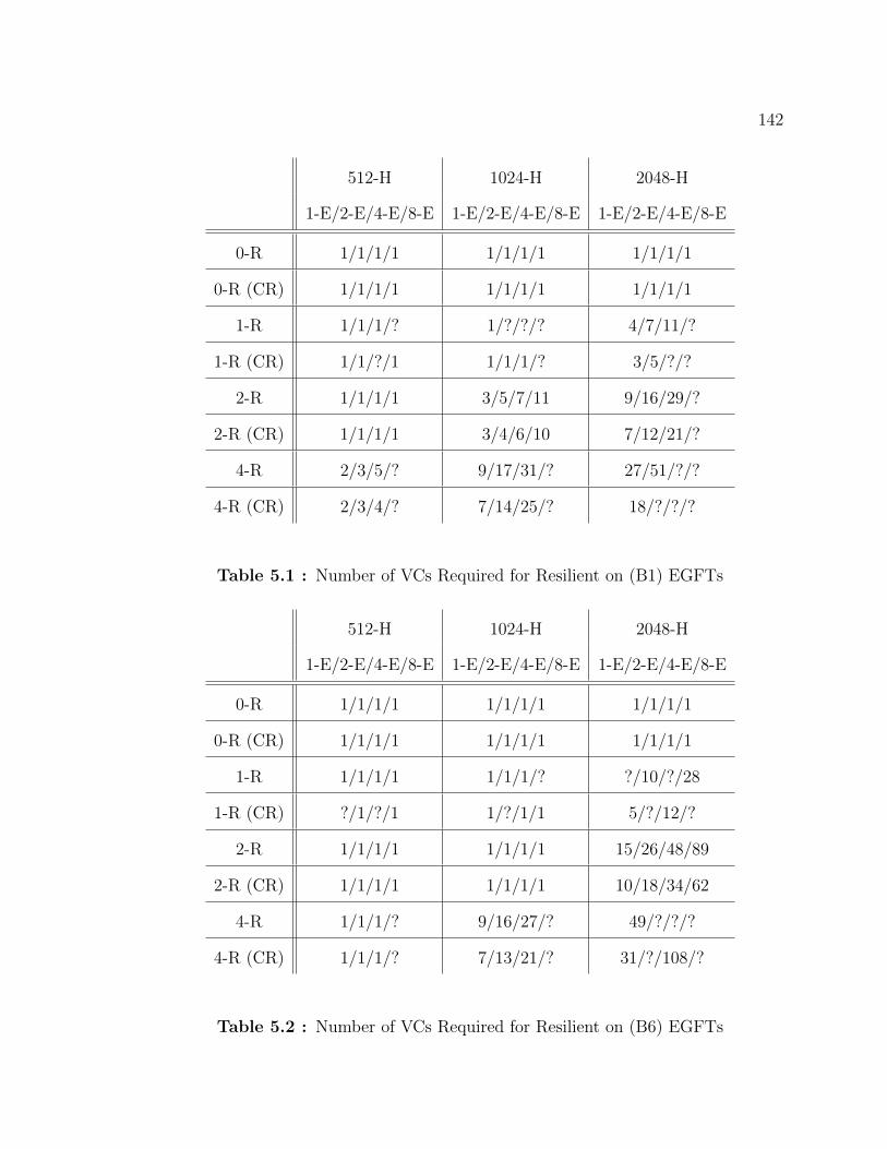
142
512-H 1024-H 2048-H
1-E/2-E/4-E/8-E 1-E/2-E/4-E/8-E 1-E/2-E/4-E/8-E
0-R 1/1/1/1 1/1/1/1 1/1/1/1
0-R (CR) 1/1/1/1 1/1/1/1 1/1/1/1
1-R 1/1/1/? 1/?/?/? 4/7/11/?
1-R (CR) 1/1/?/1 1/1/1/? 3/5/?/?
2-R 1/1/1/1 3/5/7/11 9/16/29/?
2-R (CR) 1/1/1/1 3/4/6/10 7/12/21/?
4-R 2/3/5/? 9/17/31/? 27/51/?/?
4-R (CR) 2/3/4/? 7/14/25/? 18/?/?/?
Table 5.1 : Number of VCs Required for Resilient on (B1) EGFTs
512-H 1024-H 2048-H
1-E/2-E/4-E/8-E 1-E/2-E/4-E/8-E 1-E/2-E/4-E/8-E
0-R 1/1/1/1 1/1/1/1 1/1/1/1
0-R (CR) 1/1/1/1 1/1/1/1 1/1/1/1
1-R 1/1/1/1 1/1/1/? ?/10/?/28
1-R (CR) ?/1/?/1 1/?/1/1 5/?/12/?
2-R 1/1/1/1 1/1/1/1 15/26/48/89
2-R (CR) 1/1/1/1 1/1/1/1 10/18/34/62
4-R 1/1/1/? 9/16/27/? 49/?/?/?
4-R (CR) 1/1/1/? 7/13/21/? 31/?/108/?
Table 5.2 : Number of VCs Required for Resilient on (B6) EGFTs

143
To be more specific, Table 5.1 and Table 5.2 show the required number of virtual
channels on the (B1) and (B6) EGFT topologies, respectively, for varying topology
sizes (*-H), levels of resilience (*-R), and degrees of multipathing (*-E). First, these
tables show that the virtual channel assignment algorithm always finds an assignment
for 0-resilience that only requires one virtual channel, which is expected as prior work
has shown that minimal routing on fat trees is deadlock-free [23]. Although expected,
this at least verifies my implementation of the channel assignment algorithm.
These tables also show that compression-aware routing can reduce the number
of required virtual channels, frequently requiring 1–3 fewer virtual channels than
without compression-aware routing. Although compression-aware routing starts to
significantly reduce the number of virtual channels when DF-FI resilience already
requires tens of virtual channels, often requiring 5–20 fewer virtual channels, this
result is not that significant because DF-FI resilience with compression-aware routing
still requires far more trees than are currently available in these cases.
Next, these tables show that the number of virtual channels required by DF-FI
resilience is in fact prohibitive. Providing even 8-way ECMP and 4-resilience required
10 or more virtual channels even on all of the 1024-host topologies I evaluated. Sim-
ilarly, 4-way ECMP and 1-resilience requires 10 or more trees on all of the 2048-host
topologies I evaluated, and 1-way ECMP and 2-resilience is barely implementable on
the 2048-host topologies I evaluated, typically requiring 8 virtual channels. These
results imply that DF-FI resilience does not scale given the currently available num-
ber of virtual channels to networks larger than 2048-hosts or levels of resilience larger
than 1–2, even if performance is compromised by reducing the degree of multipathing.
To illustrate that these results hold on other topologies, Table 5.3 shows the num-
ber of required virtual channels on the (B1) Jellyfish topologies. Although minimal
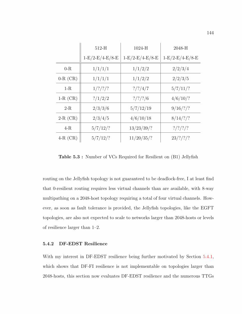
144
512-H 1024-H 2048-H
1-E/2-E/4-E/8-E 1-E/2-E/4-E/8-E 1-E/2-E/4-E/8-E
0-R 1/1/1/1 1/1/2/2 2/2/3/4
0-R (CR) 1/1/1/1 1/1/2/2 2/2/3/5
1-R 1/?/?/? ?/?/4/7 5/7/11/?
1-R (CR) ?/1/2/2 ?/?/?/6 4/6/10/?
2-R 2/3/3/6 5/7/12/19 9/16/?/?
2-R (CR) 2/3/4/5 4/6/10/18 8/14/?/?
4-R 5/7/12/? 13/23/39/? ?/?/?/?
4-R (CR) 5/7/12/? 11/20/35/? 23/?/?/?
Table 5.3 : Number of VCs Required for Resilient on (B1) Jellyfish
routing on the Jellyfish topology is not guaranteed to be deadlock-free, I at least find
that 0-resilient routing requires less virtual channels than are available, with 8-way
multipathing on a 2048-host topology requiring a total of four virtual channels. How-
ever, as soon as fault tolerance is provided, the Jellyfish topologies, like the EGFT
topologies, are also not expected to scale to networks larger than 2048-hosts or levels
of resilience larger than 1–2.
5.4.2 DF-EDST Resilience
With my interest in DF-EDST resilience being further motivated by Section 5.4.1,
which shows that DF-FI resilience is not implementable on topologies larger than
2048-hosts, this section now evaluates DF-EDST resilience and the numerous TTGs

145
that I have introduced. Unlike EDST resilience, DF-EDST resilience presents a clear
trade-off between performance and fault tolerance. Given this, the key question that
I would like to answer in this chapter is as follows: What exactly does the trade-
off between performance and resilience look like? Further, because it is likely that
more than a small performance reduction when compared with reactive shortest path
routing (< 10–15%) would be unacceptable in data center networks, I would also
like to answer the following question: What is the highest level of resilience and the
smallest expected probability of routing failure that can be provided by DF-EDST
resilience without significantly impacting forwarding throughput?
To answer these questions, I evaluate the aggregate throughput, stretch, expected
probability of routing failure, and forwarding table state requirements of different
variants of all of the TTGs discussed in Section 5.2.2. Specifically, there is only one
variant of the NoRes, NoDFR, and Line topologies, even if only a subset of the TTG is
installed for each destination. However, there are multiple variants of the T, ALayer,
MLayer, Rand, and Max TTGs that I evaluated.
All things considered, I conclude that even if no further impact on throughput is
tolerable, then fault tolerance can still be improved by about an order of magnitude,
although such a forwarding table is 0-resilient. However, even providing 3-resilience
routing often has a total reduction in forwarding table from shortest path routing of
between 5–10%, and 3-resilience can prevent 3–4 orders of magnitude fewer routing
failures given 16 edge failures than non-fault-tolerant routing.
The variants of the T, ALayer, and MLayer TTGs that I evaluate have varying
layer-0 widths, with the number of trees in layer-0 determining the number of trees in
the remaining layers in each of these topologies. Because I frequently need to install
a subset of the TTG for each destination, I also vary the maximum number of trees in

146
the subset that may be in layer-0. Together, these two variables determine the trade-
off between performance and throughput on these TTGs, which leads to the following
question: what is the best value for these variables on the topologies I evaluate? I also
look at variants of these topologies that include intra-layer connections, and I look
at two different intra-layer tree orderings, “res” and “perf”. By how much do these
connections increase fault tolerance, and by how much do they hurt performance, if
any? Are the “res” and “perf” orderings noticeably different, and if so, which is more
desirable? Lastly, all of these TTGs are just variants of layered TTGs. Is one of these
TTGs obviously better than the others, or do different variants of each TTG present
desirable points in the design space?
I find that, to provide the best performance, only at most a quarter to a third the
total EDSTs in these TTGs should be set aside for resilience and not included in layer-
0 as an initial tree. To provide some context, the topologies that I evaluated have
between 10–22 trees available, with the number of trees decreasing with bisection
bandwidth. The reason only a handful of EDSTs should be set aside is because
reserving more trees starts to have a significant impact on throughput. Further, I find
that using a self-connected layer-0 improves fault tolerance without any noticeable
impact on forwarding throughput. Similarly, I find that neither the “res” or “perf”
ordering outperforms the other, either in terms of performance or fault tolerance.
Lastly, I find that the T TTG is clearly superior to either the ALayer or MLayer
TTGs.
The variants on the Rand and Max TTGs I evaluate have different levels of guar-
anteed resilience as well as two different orderings of the remaining trees, “res” and
“perf”. At what point does providing more guaranteed resilience hurt the performance
of forwarding? Is this point different for the two different orderings, and which order-

147
ing is more desirable? Does the likely lower connectivity of the Rand TTG increase
performance or hurt resilience when compared with the Max TTG, and which TTG
is more desirable?
From my evaluation, I find the following. If all trees in the Rand and Max TTGs
are initial trees, then fault tolerance is improved without even impacting performance.
However, even reserving a single tree for resilience in these TTGs begins to have a
noticeable, albeit slight impact on throughput. I also find that neither the “perf”
or “res” orderings nor the Rand or Max TTG differ significantly from one another
in terms of throughput, expected probability of routing failure, or forwarding table
state.
The Line and layered TTGs and the Rand and Max TTGs represent different
points in the TTG design space with regards to guaranteed resilience and expected
fault tolerance. Ultimately, is one of these TTGs more desirable than the others? In
response to this question, I ultimately conclude that the self-connected T TTG and
the Rand and Max TTGs are all equally desirable as the best performing variants of
all of these lead to TTGs that are similar or isomorphic.
Finally, forwarding table state may be reduced by either reducing the size of the
TTG subset for each destination or by reducing the number of different TTGs on
different virtual channels used to increased forwarding throughput, i.e., reducing the
degree of multipathing. Is one of these methods more desirable than another?
With respect to this question, I find that neither is inherently better than another.
For example, I found that using 12 trees per destination and 4-way multipathing (4
virtual channels) had aggregate forwarding throughput and forwarding table state
and only slightly reduced probability of routing failure when compared with using
8 trees per destination and 8-way multipathing (8 virtual channels). This result is

148
particularly interesting because it implies that not all of the available virtual channels
are required for high performance and fault tolerant deadlock-free routing.
In the rest of this section, I first present my results from the NoRes, NoDFR, and
Line TTGs. After that, I present my results from each of the individual layered TTGs
and then compare the layered TTGs against each other. Similarly, I need present my
results from the Rand and Max TTGs and then compare them. After that, I compare
and discuss the best variants of the TTGs that were previously presented.
NoRes, NoDFR, and Line TTGs
In this section, I first look at the probability of routing failure, throughput, and state
requirements of the NoRes, NoDFR, and Line TTGs. While none of these TTGs
are practical for providing high throughput deadlock-free and fault-tolerant routing.
However, they are still interesting, nonetheless as the NoRes TTG provides a lower
bound on both fault tolerance and forwarding table state, the NoDFR TTG provides
an upper bound on both fault tolerance of tree resilience and forwarding table state,
and the Line TTG provides an upper bound on the fault tolerance achievable given
deadlock-free routing.
Further, these TTGs also illustrate that the forwarding table state required by
naively using all available trees per destination and all available virtual channels in
DF-EDST resilience requires too much forwarding table state. Two ways to reduce
this state are by reducing the size of the subset of the TTG installed per destination
or by reducing the degree of multipathing, and I use the NoRes, NoDFR, and Line
TTGs to illustrate the pros and cons of both approaches. Specifically, I find that, in
addition to increasing resilience and fault tolerance, increasing the number of trees
per destination can also improve performance. This is because the number of initial

149
trees are increased as well, although this effect reaches a plateau eventually because
the shortest trees, averaged across all switches, are chosen for the subset of the TTG.
For example, the NoRes and NoDFR TTGs with 8-trees and 8-way multipathing are
not far off of the throughput of reactive, deadlock-oblivious shortest path routing.
On the other hand, multipathing does not impact fault tolerance, but decreasing the
degree of multipathing by half almost reduces aggregate throughput by half as well.
Because of these results and because DF-EDST resilience is intended for data center
networks, where performance is critical and routing over EDSTs already has a small
impact on performance [35], I only consider variants of the other TTGs that have the
maximal possible degree of multipathing, 8, which is equal to the number of virtual
channels.
To concretely illustrate the state requirements of DF-EDST resilience, Figure 5.8
and Figure 5.9 show the state requirements of variants of the NoRes, NoDFR, and Line
TTGs with different number of trees installed per destination (*-T) and degrees of
multipath (*-E) given different topologies, topology sizes, and bisection bandwidths
(B*). Although there are more than 20 EDSTs in the TTG for the 1 : 1 bisection
bandwidth topologies, this figure shows that even with only 8 trees per destination and
8-way multipathing, the largest possible, that the NoDFR requires 40Mbit of TCAM
even on hosts with between 2048–4096 hosts. However, the NoDFR TTG requires
more state than any deadlock-free TTG, with the 8 trees and 8-way multipathing
on the Line TTG requiring 40Mbit of TCAM for networks with between 4096–8192
hosts. On the other hand, because NoRes does not install rules to allow packets to
transition between trees, it requires the least forwarding table state and should scale
to at least 10K hosts given 40Mbit of TCAM state, 8-trees per destination, and 8-way
multipathing.

150
210 211 212
Number of Hosts
104
TCAM
Siz
e (K
b)
Line 16-T 8-ENoDFR 8-T 8-ELine 12-T 8-ELine 16-T 4-E
NoDFR 8-T 4-ELine 12-T 4-ELine 8-T 8-ENoDFR 4-T 8-E
Line 8-T 4-ENoRes 8-T 8-ENoDFR 4-T 4-ELine 4-T 8-E
NoRes 8-T 4-ENoRes 4-T 8-ELine 4-T 4-ENoRes 4-T 4-E
(a) Network Virtualization (B1)
210 211 212 213
Number of Hosts
103
104
TCAM
Siz
e (K
b)
Line 16-T 8-ENoDFR 8-T 8-ELine 12-T 8-ELine 16-T 4-E
NoDFR 8-T 4-ELine 12-T 4-ELine 8-T 8-ENoDFR 4-T 8-E
Line 8-T 4-ENoRes 8-T 8-ENoDFR 4-T 4-ELine 4-T 8-E
NoRes 8-T 4-ENoRes 4-T 8-ELine 4-T 4-ENoRes 4-T 4-E
(b) Network Virtualization (B2)
Figure 5.8 : Jellyfish TCAM Sizes for the NoRes, NoDFR, and Line TTGs

151
210 211 212
Number of Hosts
103
104
TCAM
Siz
e (K
b)
Line 16-T 8-ENoDFR 8-T 8-ELine 12-T 8-ELine 16-T 4-E
NoDFR 8-T 4-ELine 12-T 4-ELine 8-T 8-ENoDFR 4-T 8-E
Line 8-T 4-ENoRes 8-T 8-ENoDFR 4-T 4-ELine 4-T 8-E
NoRes 8-T 4-ENoRes 4-T 8-ELine 4-T 4-ENoRes 4-T 4-E
(a) Network Virtualization (B1)
210 211 212 213
Number of Hosts
103
104
TCAM
Siz
e (K
b)
NoDFR 8-T 8-ENoDFR 8-T 4-ELine 16-T 8-ELine 12-T 8-E
Line 16-T 4-ELine 12-T 4-ELine 8-T 8-ENoDFR 4-T 8-E
Line 8-T 4-ENoRes 8-T 8-ENoDFR 4-T 4-ELine 4-T 8-E
NoRes 8-T 4-ENoRes 4-T 8-ELine 4-T 4-ENoRes 4-T 4-E
(b) Network Virtualization (B2)
210 211 212 213
Number of Hosts
103
104
TCAM
Siz
e (K
b)
NoDFR 8-T 8-ELine 9-T 8-ELine 12-T 8-ENoDFR 8-T 4-E
Line 12-T 4-ELine 8-T 8-ELine 9-T 4-ENoDFR 4-T 8-E
Line 8-T 4-ENoRes 8-T 8-ENoDFR 4-T 4-ELine 4-T 8-E
NoRes 8-T 4-ENoRes 4-T 8-ELine 4-T 4-ENoRes 4-T 4-E
(c) Network Virtualization (B4)
Figure 5.9 : EGFT TCAM Sizes for the NoRes, NoDFR, and Line TTGs

152
20 21 22 23 24 25 26 27 28
Number of Failures10-9
10-8
10-7
10-6
10-5
10-4
10-3
Frac
tion
ofFl
ows
Faile
d
NoRes 4-T 4-ENoRes 8-T 4-ENoRes 4-T 8-ENoRes 8-T 8-E
Line 4-T 4-ELine 4-T 8-ENoDFR 4-T 4-ENoDFR 4-T 8-E
Line 8-T 4-ELine 8-T 8-ELine 12-T 4-ENoDFR 8-T 4-E
Line 16-T 8-ELine 12-T 8-ENoDFR 8-T 8-ELine 16-T 4-E
(a) 1024-hosts (B1)
20 21 22 23 24 25 26 27 28
Number of Failures10-9
10-8
10-7
10-6
10-5
10-4
10-3
Frac
tion
ofFl
ows
Faile
d
NoRes 4-T 8-ENoRes 8-T 8-ELine 4-T 4-E
Line 4-T 8-ENoDFR 4-T 8-ELine 8-T 4-E
Line 8-T 8-ENoDFR 8-T 8-ELine 12-T 4-E
Line 16-T 8-ELine 12-T 8-ELine 16-T 4-E
(b) 1024-hosts (B2)
20 21 22 23 24 25 26 27 28
Number of Failures10-9
10-8
10-7
10-6
10-5
10-4
10-3
Frac
tion
ofFl
ows
Faile
d
NoRes 4-T 8-ENoRes 8-T 8-ELine 4-T 4-E
Line 4-T 8-ENoDFR 4-T 8-ELine 8-T 4-E
Line 8-T 8-ELine 12-T 4-ELine 16-T 8-E
Line 12-T 8-ELine 16-T 4-ENoDFR 8-T 8-E
(c) 2048-hosts (B2)
20 21 22 23 24 25 26 27 28
Number of Failures10-8
10-7
10-6
10-5
10-4
10-3
Frac
tion
ofFl
ows
Faile
d
NoRes 4-T 8-ENoRes 8-T 8-ELine 12-T 4-E
Line 4-T 8-ELine 12-T 8-ELine 4-T 4-E
NoDFR 4-T 8-ELine 8-T 4-E
Line 8-T 8-ENoDFR 8-T 8-E
(d) 2048-hosts (B4)
Figure 5.10 : Jellyfish Probability of Routing Failure for the NoRes, NoDFR, and
Line TTGs
Further, these figures also show that reducing the number of trees per destination
reduces forwarding table state by more than reducing the degree of multipathing. For
example, Line 4-T 8-E reduces the forwarding table state of Line 8-T 8-E by about
twice as much as Line 8-T 4-E. However, this is expected state in DF-EDST resilience
is still super-linear with respect to the number of trees, while forwarding table state
clearly changes linearly with respect to changes in the degree of multipathing.

153
20 21 22 23 24 25 26 27 28
Number of Failures10-9
10-8
10-7
10-6
10-5
10-4
10-3
Frac
tion
ofFl
ows
Faile
d
NoRes 4-T 4-ENoRes 8-T 4-ENoRes 4-T 8-ENoRes 8-T 8-E
Line 4-T 4-ELine 4-T 8-ENoDFR 4-T 4-ENoDFR 4-T 8-E
Line 8-T 4-ELine 8-T 8-ELine 12-T 4-ENoDFR 8-T 4-E
Line 16-T 8-ELine 12-T 8-ENoDFR 8-T 8-ELine 16-T 4-E
(a) 1024-hosts (B1)
20 21 22 23 24 25 26 27 28
Number of Failures10-8
10-7
10-6
10-5
10-4
10-3
Frac
tion
ofFl
ows
Faile
d
NoRes 4-T 4-ENoRes 8-T 4-ENoRes 4-T 8-ENoRes 8-T 8-E
Line 4-T 4-ELine 4-T 8-ENoDFR 4-T 8-ENoDFR 4-T 4-E
Line 12-T 4-ELine 8-T 4-ELine 8-T 8-ENoDFR 8-T 4-E
Line 16-T 8-ELine 12-T 8-ENoDFR 8-T 8-ELine 16-T 4-E
(b) 1024-hosts (Correlated) (B1)
20 21 22 23 24 25 26 27 28
Number of Failures10-8
10-7
10-6
10-5
10-4
10-3
Frac
tion
ofFl
ows
Faile
d
NoRes 8-T 8-ENoRes 4-T 8-ELine 4-T 4-E
Line 4-T 8-ENoDFR 4-T 8-ELine 8-T 4-E
Line 8-T 8-ENoDFR 8-T 8-E
Line 12-T 4-ELine 12-T 8-E
(c) 1024-hosts (B2)
20 21 22 23 24 25 26 27 28
Number of Failures10-7
10-6
10-5
10-4
10-3
Frac
tion
ofFl
ows
Faile
d
NoRes 8-T 8-ENoRes 4-T 8-ELine 4-T 4-E
Line 4-T 8-ENoDFR 4-T 8-ELine 8-T 8-E
Line 8-T 4-ENoDFR 8-T 8-E
Line 12-T 8-ELine 12-T 4-E
(d) 1024-hosts (B4)
Figure 5.11 : EGFT Probability of Routing Failure for the NoRes, NoDFR, and
Line TTGs

154
Next, Figure 5.10 and Figure 5.11 show the probability of a routing failure given
Jellyfish and EGFT topologies, respectively, different numbers of hosts and bisection
bandwidths (B*), size of the TTG subset installed for each destination (*-T) and
degrees of multipathing (*-E). As before, the lines in the legend are sorted from least
fault tolerant to most.
The first thing that these figures show is that, as expected, using more or less
TTGs on different virtual channels does not impact fault tolerance. Because the
routing functions of each TTG are independent and the TTGs themselves are identical
for each virtual channel, the exact number of virtual channels used should only impact
state and forwarding throughput, as, to increased path diversity, the EDSTs used for
each virtual channel are selected so that they are all different.
Next, these figures also show that changing the size of the subset of the TTG
installed for each destination does impact fault tolerance, which, again, is expected.
Except for the NoRes TTG, which does allow for packets to transition between trees,
the more trees there are, the higher the fault tolerance.
Perhaps surprisingly, these figures show that, across a range of topologies and
bisection bandwidths, the NoDFR TTG consistently achieves higher fault tolerance
than the comparable Line TTG, even though both TTGs provide the same guaranteed
resilience. This is because the NoDFR may, for each switch, destination, and failure,
chosen the shortest non-failed tree while the Line TTG must use the next non-failed
tree in the TTG when a failure is encountered. This leads to longer paths, in practice,
and the longer path a packet is forwarded over, the more likely it is then to encounter
a failure. This is especially notable in Figure 5.11a, where NoDFR with 8-trees
per destination is slightly more fault tolerant than the Line TTG with 16-trees per
destination, although, given either correlated failures (Figure 5.11b) or lower bisection

155
20 21 22 23 24 25 26 27 28
Number of Failures0.10.20.30.40.50.60.70.80.9
Norm
aliz
ed T
hrou
ghpu
t
SPNoDFR 8-T 8-ENoRes 8-T 8-ENoDFR 8-T 4-ENoDFR 4-T 8-E
NoRes 4-T 8-ENoRes 8-T 4-ENoDFR 4-T 4-ENoRes 4-T 4-E
Line 4-T 8-ELine 8-T 8-ELine 12-T 8-ELine 16-T 8-E
Line 4-T 4-ELine 8-T 4-ELine 12-T 4-ELine 16-T 4-E
(a) 2048-hosts (B1)
210 211 212
Number of Hosts0.10.20.30.40.50.60.70.80.9
Norm
aliz
ed T
hrou
ghpu
t
SPNoDFR 8-T 8-ENoRes 8-T 8-ENoDFR 4-T 8-ENoDFR 8-T 4-E
NoRes 4-T 8-ENoRes 8-T 4-ENoDFR 4-T 4-ENoRes 4-T 4-E
Line 4-T 8-ELine 8-T 8-ELine 12-T 8-ELine 16-T 8-E
Line 4-T 4-ELine 8-T 4-ELine 12-T 4-ELine 16-T 4-E
(b) 16-F (B1)
20 21 22 23 24 25 26 27 28
Number of Failures0.20.30.40.50.60.70.80.9
Norm
aliz
ed T
hrou
ghpu
t
SPNoRes 8-T 8-ENoDFR 8-T 8-ENoRes 8-T 4-ENoDFR 8-T 4-E
NoRes 4-T 8-ENoDFR 4-T 8-ENoRes 4-T 4-ENoDFR 4-T 4-E
Line 4-T 8-ELine 8-T 8-ELine 12-T 8-ELine 16-T 8-E
Line 4-T 4-ELine 8-T 4-ELine 12-T 4-ELine 16-T 4-E
(c) 1024-hosts (B2)
210 211 212 213
Number of Hosts0.10.20.30.40.50.60.70.80.9
Norm
aliz
ed T
hrou
ghpu
t
SPNoRes 8-T 8-ENoDFR 8-T 8-ENoRes 8-T 4-ENoDFR 8-T 4-E
NoDFR 4-T 8-ENoRes 4-T 8-ENoRes 4-T 4-ENoDFR 4-T 4-E
Line 4-T 8-ELine 8-T 8-ELine 12-T 8-ELine 16-T 8-E
Line 4-T 4-ELine 8-T 4-ELine 12-T 4-ELine 16-T 4-E
(d) 16-F (B2)
Figure 5.12 : Jellyfish Throughput for the NoRes, NoDFR, and Line TTGs
bandwidth networks (Figure 5.11c and Figure 5.11d), variants of the Line TTG with
more trees than a variant of the NoDFR TTG begin to out-perform the NoDFR
variant.
Next, Figure 5.12 and Figure 5.13 present the throughput of the Jellyfish and
EGFT topologies, respectively, given different topology sizes, numbers of failures (*-
F), bisection bandwidths, and variants of the NoRes, NoDFR, and Line TTGs.
First, these figures show that the NoRes TTG provides high aggregate throughput

156
20 21 22 23 24 25 26 27 28
Number of Failures0.10.20.30.40.50.60.70.8
Norm
aliz
ed T
hrou
ghpu
t
SPNoRes 8-T 8-ENoDFR 8-T 8-ENoRes 4-T 8-ENoRes 8-T 4-E
NoDFR 8-T 4-ENoDFR 4-T 8-ENoDFR 4-T 4-ENoRes 4-T 4-E
Line 4-T 8-ELine 8-T 8-ELine 12-T 8-ELine 16-T 8-E
Line 4-T 4-ELine 8-T 4-ELine 12-T 4-ELine 16-T 4-E
(a) 2048-hosts (B1)
210 211 212
Number of Hosts0.10.20.30.40.50.60.70.8
Norm
aliz
ed T
hrou
ghpu
tSPNoRes 8-T 8-ENoDFR 8-T 8-ENoDFR 4-T 8-E
NoDFR 8-T 4-ENoRes 4-T 8-ENoRes 8-T 4-ENoDFR 4-T 4-E
NoRes 4-T 4-ELine 4-T 8-ELine 8-T 8-ELine 12-T 8-E
Line 4-T 4-ELine 8-T 4-ELine 12-T 4-ELine 16-T 4-E
(b) 16-F (B1)
210 211 212 213
Number of Hosts0.1
0.2
0.3
0.4
0.5
Norm
aliz
ed T
hrou
ghpu
t
SPNoRes 8-T 8-ENoDFR 8-T 8-ENoRes 8-T 4-ENoDFR 8-T 4-E
NoDFR 4-T 8-ENoRes 4-T 8-ENoDFR 4-T 4-ENoRes 4-T 4-E
Line 4-T 8-ELine 8-T 8-ELine 12-T 8-ELine 16-T 8-E
Line 4-T 4-ELine 8-T 4-ELine 12-T 4-ELine 16-T 4-E
(c) 16-F (B2)
210 211 212 213
Number of Hosts0.10
0.15
0.20
0.25
0.30
0.35
0.40
Norm
aliz
ed T
hrou
ghpu
t
SPNoDFR 8-T 8-ENoRes 8-T 8-ENoRes 8-T 4-E
NoDFR 8-T 4-ENoDFR 4-T 8-ENoRes 4-T 8-E
NoRes 4-T 4-ENoDFR 4-T 4-ELine 4-T 8-E
Line 8-T 8-ELine 4-T 4-ELine 8-T 4-E
(d) 16-F (B4)
Figure 5.13 : EGFT Throughput for the NoRes, NoDFR, and Line TTGs

157
that begins to gradually fall off of the throughput of shortest path routing (SP) as
topology size increases, which agrees with previous work [35]. Similarly, these figures
also show that the aggregate throughput of the NoDFR TTG is very similar to that
of the NoRes TTG on all of the topologies and number of failures I considered.
On the other hand, these figures also illustrate the key problem with the Line TTG.
Even if only a subset of the TTG is installed for each destination, and the subset of
the shortest trees is chosen for a destination, there is still not enough path diversity
provided by the set of initial trees to ensure high throughput forwarding even when
there are no failures. In these figures, the aggregate forwarding throughput achieved
by the Line TTG was typically almost half that of shortest path forwarding. Although
this performance impact is reduced on networks with lower bisection bandwidths, such
as Figure 5.13d, the performance impact is still significant. Further, these figures have
the surprising trend that the fewer the number of trees installed for each destination,
the higher the throughput. This is because all forwarding starts at the topologically
first tree in the TTG, so the larger the subset, the smaller the number of initial trees.
These figures also show the second half of the trade-off between reducing the
number of trees installed per destination or reducing the number of virtual channels
used for multipathing. While I have already shown that increasing the number of
trees not only increases resilience but also has a significant impact on fault tolerance,
these figures show that reducing the degree of multipathing has a significant impact
on performance. However, these figures also show that the number of trees can impact
performance. For example, both the “4-T 8-E” and “8-T 4-E” variants of the NoDFR
and NoRes reduced forwarding throughput by the same amount. This is because both
variants reduce the number of initial forwarding trees by the same amount. However,
decreasing the number of trees on the Line TTG, which increases the number of initial

158
trees, has less impact on throughput than reducing the degree of multipathing.
Layered TTGs
Next, I look at the T, ALayer, and MLayer TTGs, which together form the layered
TTGs. I consider these TTGs because they provide similar resilience for all initial
trees yet have more initial trees than the Line TTG so as to provide better forwarding
throughput. In this evaluation, I first consider variants of the T TTG, which clearly
illustrates the trade-off between performance and resilience as it either uses a tree as
an initial tree for good throughput or reserves it for resilience as part of a line. In
addition to evaluating the aggregate throughput, probability of routing failure, and
forwarding table state required by the T TTG, I also evaluate whether allowing for
the first layer to be self-connected hurts performance of significantly improves fault
tolerance, finding that it improves fault tolerance without hurting performance. After
that, I then see if variants of either the ALayer or MLayer TTG outperform the T
TTG in terms of either fault tolerance or forwarding throughput, and the answer
to this question is clear. The ALayer and MLayer TTGs perform nearly identically
to the T TTG, yet provide less fault tolerance. This implies that the performance
of backup routes is not crucial to overall performance, and so that non-initial trees
should be arranged in a line so as to provide the best fault tolerance.
To start off, Figure 5.14 and Figure 5.15 show the probability of routing failure
given the T and ALayer TTG, the the MLayer TTG being omitted because it fell
somewhere inbetwen the two. To allow for comparisons between different variants
of the TTGs, I fix the both the number of subtrees per destination and degree of
multipathing at 8 in these figures. In these figures, I vary both the width of the layer-
0 of the TTG ({T,AL}-*) and the maximum number of trees in the subset of the

159
23 24 25 26 27 28
Number of Failures10-7
10-6
10-5
Frac
tion
ofFl
ows
Faile
d
NoResT-16 6-L0T-12 6-L0T-16 5-L0T-12 5-L0
T-16 6-L0 (SL-R)T-8 6-L0T-8 5-L0T-16 4-L0T-12 6-L0 (SL-R)
T-12 4-L0T-16 5-L0 (SL-R)T-12 5-L0 (SL-R)T-8 4-L0T-16 4-L0 (SL-R)
T-8 6-L0 (SL-R)T-8 5-L0 (SL-R)T-8 4-L0 (SL-R)T-12 4-L0 (SL-R)NoDFR
(a) 1024-hosts T TTG (B1)
23 24 25 26 27 28
Number of Failures10-7
10-6
10-5
Frac
tion
ofFl
ows
Faile
d
AL-16 6-L0AL-12 6-L0AL-16 5-L0AL-12 5-L0AL-16 4-L0
AL-12 4-L0AL-8 6-L0AL-8 5-L0AL-8 4-L0AL-16 6-L0 (SL-R)
AL-12 6-L0 (SL-R)AL-16 5-L0 (SL-R)AL-12 5-L0 (SL-R)AL-8 5-L0 (SL-R)
AL-8 6-L0 (SL-R)AL-16 4-L0 (SL-R)AL-8 4-L0 (SL-R)AL-12 4-L0 (SL-R)
(b) 1024-hosts ALayer TTG (B1)
20 21 22 23 24 25 26 27 28
Number of Failures10-9
10-8
10-7
10-6
10-5
10-4
10-3
Frac
tion
ofFl
ows
Faile
d
NoResT-16 4-L0T-16 6-L0
T-16 5-L0T-12 6-L0
T-12 5-L0T-8 6-L0
T-8 5-L0T-12 4-L0
T-8 4-L0NoDFR
(c) 1536-hosts T TTG (B2)
20 21 22 23 24 25 26 27 28
Number of Failures10-9
10-8
10-7
10-6
10-5
10-4
10-3
Frac
tion
ofFl
ows
Faile
d
AL-16 5-L0AL-16 6-L0
AL-16 4-L0AL-12 6-L0
AL-12 5-L0AL-12 4-L0
AL-8 6-L0AL-8 5-L0
AL-8 4-L0
(d) 1536-hosts ALayer TTG (B2)
210 211 212
Number of Hosts10-10
10-9
10-8
10-7
10-6
10-5
10-4
Frac
tion
ofFl
ows
Faile
d
NoResT-16 4-L0T-16 6-L0
T-16 5-L0T-12 6-L0
T-8 6-L0T-12 5-L0
T-8 5-L0T-8 4-L0
T-12 4-L0NoDFR
(e) 64-F T TTG (B2)
210 211 212
Number of Hosts10-8
10-7
10-6
10-5
Frac
tion
ofFl
ows
Faile
d
AL-16 4-L0AL-16 5-L0
AL-16 6-L0AL-12 6-L0
AL-12 5-L0AL-12 4-L0
AL-8 6-L0AL-8 5-L0
AL-8 4-L0
(f) 64-F ALayer TTG (B2)
Figure 5.14 : Jellyfish Probability of Routing Failure for the T and ALayer TTGs

160
23 24 25 26 27 28
Number of Failures
10-6
10-5
Frac
tion
ofFl
ows
Faile
d
NoResT-16 6-L0T-12 6-L0T-16 4-L0T-16 5-L0
T-12 5-L0T-16 6-L0 (SL-R)T-8 6-L0T-8 5-L0T-12 6-L0 (SL-R)
T-16 5-L0 (SL-R)T-16 4-L0 (SL-R)T-12 4-L0T-12 5-L0 (SL-R)T-8 6-L0 (SL-R)
T-8 4-L0T-12 4-L0 (SL-R)T-8 5-L0 (SL-R)T-8 4-L0 (SL-R)NoDFR
Figure 5.15 : Probability of Routing Failure for the 1024-host (B1) EGFT Topology
and the T TTG
TTG for each destination (*-ML0) as well as consider variants of the TTG that use
a self-connected layer-0 with rules sorted for both performance (SL-P) or resilience
(SL-R). In effect, the width of the layer-0 of the TTG sets a global limit on the
number of initial trees and resilience while the maximum number of trees per subset
sets a limit on fault tolerance of each subset to avoid trivially choosing a subset that
is only composed of initial trees and thus not different from the NoRes TTG.
First, I note that the probability of routing failure on the ALayer TTG was always
either equal or greater than on the T TTG. This is expected because the T TTG is
likely to have a larger height than an equivalent variant of the MLayer or ALayer
TTG, and thus is likely to be more resilient.
Next, I note that, while allowing for a self-connected layer-0 can noticeably im-
prove fault tolerance, neither variant of sorting the rules in the self-connected layer

161
dominated the other. This may be because I sort the initial trees of the TTG by path
length averaged over all switches and destinations before connecting them, so both
orderings may be similar. Because of this, I only show the results from the resilient
sorting (SL-R). Additionally, these figures show the overall trend that reducing either
the layer-0 width or the maximum number of layer-0 cause similar increases in fault
tolerance. Although the difference between each individual variant may not be that
large, the probability of routing failure on the 1024-host topologies in Figure 5.14a
Figure 5.15 differ by almost two orders of magnitude given 64 edge failures. How-
ever, except for the variants that have a layer-0 width of 16 on the (B2) topologies
(Figure 5.14c and Figure 5.14e), which is roughly the total number of EDSTs, all
of the variants provide a significant increase in fault tolerance when compared with
non-fault-tolerant routing (NoRes), although none of them match the performance
of the NoDFR TTG, which did not experience any routing failures given 64 edges
failures on the 1024-host topologies.
Next, Figure 5.16 and Figure 5.17 show the aggregate throughput achieved by
different variants of the T and ALayer TTGs on the Jellyfish and EGFT topology,
respectively. Most importantly, these figures show that, unlike the line TTG, the T
and ALayer TTGs have enough initial trees to provide high throughput forwarding.
In these figures, the throughput of the best performing T TTGs is often within a
factor of 10% of that of reactive, deadlock-oblivious shortest path routing, which I
note already achieves a little bit higher forwarding throughput than using EDSTs for
deadlock-free routing (NoRes) [35]. Although the forwarding throughput falls off of
that of shortest path routing as the number of failures increases (> 32), this is likely
acceptable as the liklihood of this many edges failing at once is low [5].
Next, these figures show that there is little benefit to the ALayer or MLayer TTGs.
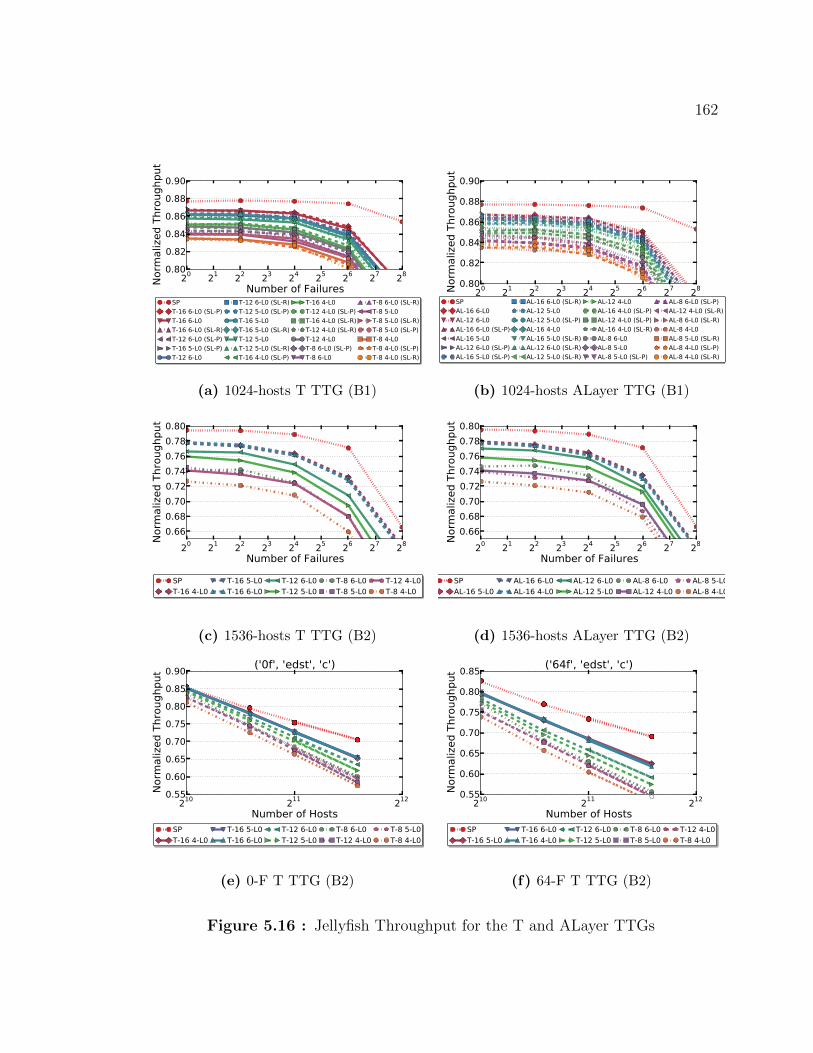
162
20 21 22 23 24 25 26 27 28
Number of Failures0.800.820.840.860.880.90
Norm
aliz
ed T
hrou
ghpu
t
SPT-16 6-L0 (SL-P)T-16 6-L0T-16 6-L0 (SL-R)T-12 6-L0 (SL-P)T-16 5-L0 (SL-P)T-12 6-L0
T-12 6-L0 (SL-R)T-12 5-L0 (SL-P)T-16 5-L0T-16 5-L0 (SL-R)T-12 5-L0T-12 5-L0 (SL-R)T-16 4-L0 (SL-P)
T-16 4-L0T-12 4-L0 (SL-P)T-16 4-L0 (SL-R)T-12 4-L0 (SL-R)T-12 4-L0T-8 6-L0 (SL-P)T-8 6-L0
T-8 6-L0 (SL-R)T-8 5-L0T-8 5-L0 (SL-R)T-8 5-L0 (SL-P)T-8 4-L0T-8 4-L0 (SL-P)T-8 4-L0 (SL-R)
(a) 1024-hosts T TTG (B1)
20 21 22 23 24 25 26 27 28
Number of Failures0.80
0.82
0.84
0.86
0.88
0.90
Norm
aliz
ed T
hrou
ghpu
t
SPAL-16 6-L0AL-12 6-L0AL-16 6-L0 (SL-P)AL-16 5-L0AL-12 6-L0 (SL-P)AL-16 5-L0 (SL-P)
AL-16 6-L0 (SL-R)AL-12 5-L0AL-12 5-L0 (SL-P)AL-16 4-L0AL-16 5-L0 (SL-R)AL-12 6-L0 (SL-R)AL-12 5-L0 (SL-R)
AL-12 4-L0AL-16 4-L0 (SL-P)AL-12 4-L0 (SL-P)AL-16 4-L0 (SL-R)AL-8 6-L0AL-8 5-L0AL-8 5-L0 (SL-P)
AL-8 6-L0 (SL-P)AL-12 4-L0 (SL-R)AL-8 6-L0 (SL-R)AL-8 4-L0AL-8 5-L0 (SL-R)AL-8 4-L0 (SL-P)AL-8 4-L0 (SL-R)
(b) 1024-hosts ALayer TTG (B1)
20 21 22 23 24 25 26 27 28
Number of Failures
0.660.680.700.720.740.760.780.80
Norm
aliz
ed T
hrou
ghpu
t
SPT-16 4-L0
T-16 5-L0T-16 6-L0
T-12 6-L0T-12 5-L0
T-8 6-L0T-8 5-L0
T-12 4-L0T-8 4-L0
(c) 1536-hosts T TTG (B2)
20 21 22 23 24 25 26 27 28
Number of Failures
0.660.680.700.720.740.760.780.80
Norm
aliz
ed T
hrou
ghpu
t
SPAL-16 5-L0
AL-16 6-L0AL-16 4-L0
AL-12 6-L0AL-12 5-L0
AL-8 6-L0AL-12 4-L0
AL-8 5-L0AL-8 4-L0
(d) 1536-hosts ALayer TTG (B2)
210 211 212
Number of Hosts0.550.600.650.700.750.800.850.90
Norm
aliz
ed T
hrou
ghpu
t ('0f', 'edst', 'c')
SPT-16 4-L0
T-16 5-L0T-16 6-L0
T-12 6-L0T-12 5-L0
T-8 6-L0T-12 4-L0
T-8 5-L0T-8 4-L0
(e) 0-F T TTG (B2)
210 211 212
Number of Hosts0.55
0.60
0.65
0.70
0.75
0.80
0.85
Norm
aliz
ed T
hrou
ghpu
t ('64f', 'edst', 'c')
SPT-16 5-L0
T-16 6-L0T-16 4-L0
T-12 6-L0T-12 5-L0
T-8 6-L0T-8 5-L0
T-12 4-L0T-8 4-L0
(f) 64-F T TTG (B2)
Figure 5.16 : Jellyfish Throughput for the T and ALayer TTGs

163
20 21 22 23 24 25 26 27 28
Number of Failures0.600.620.640.660.680.700.720.740.76
Norm
aliz
ed T
hrou
ghpu
t
SPT-16 6-L0 (SL-P)T-16 6-L0T-16 5-L0 (SL-P)T-16 5-L0T-16 6-L0 (SL-R)T-12 6-L0 (SL-P)
T-12 6-L0T-16 4-L0T-12 5-L0 (SL-P)T-12 5-L0T-12 6-L0 (SL-R)T-16 5-L0 (SL-R)T-16 4-L0 (SL-P)
T-12 5-L0 (SL-R)T-16 4-L0 (SL-R)T-12 4-L0T-8 6-L0T-12 4-L0 (SL-P)T-12 4-L0 (SL-R)T-8 5-L0 (SL-P)
T-8 5-L0T-8 6-L0 (SL-P)T-8 4-L0T-8 6-L0 (SL-R)T-8 5-L0 (SL-R)T-8 4-L0 (SL-P)T-8 4-L0 (SL-R)
(a) 1024-hosts (B1)
20 21 22 23 24 25 26 27 28
Number of Failures0.25
0.30
0.35
0.40
0.45
0.50
Norm
aliz
ed T
hrou
ghpu
t
SPT-12 6-L0
T-12 4-L0T-12 5-L0
T-8 6-L0 T-8 5-L0 T-8 4-L0
(b) 2048-hosts (B2)
Figure 5.17 : EGFT Throughput for the T TTG
While the ALayer TTG did achieve higher throughput in some cases, namely a large
number of failures, such large failures are not frequently expected in data center
networks [5], and said benefit does not outweigh the loss of fault tolerance previously
discussed.
Further, Figure 5.16a and Figure 5.17a show that self-connecting the initial layer
does not have a significant impact on forwarding throughput. This, combined with
the increase in fault tolerance, shows that, even though self connecting the layers in
these TTGs does not increase resilience, doing so improves fault tolerance without
hurting throughput. Although using a tree that may be used for forwarding default
traffic for fault tolerance instead of one of the backup trees could be expected to
impact performance, in practice, these figures show that this is not the case. This is
most likely because using multiple virtual channels for improve performance can lead
to all of the links in the network being utilized, and moving either to another initial
tree or a tree reserved for resilience is still likely to use edges used by other flows.
However, this result on self-connected layers begins to undermine the motivation for

164
210 211
Number of Hosts
104TC
AM S
ize
(Kb)
NoDFRT-16 6-L0 (SL-R)T-16 6-L0 (SL-P)T-12 6-L0 (SL-R)T-12 6-L0 (SL-P)T-16 5-L0 (SL-P)T-16 5-L0 (SL-R)T-12 5-L0 (SL-R)
T-12 5-L0 (SL-P)T-8 5-L0 (SL-P)T-8 5-L0 (SL-R)T-8 6-L0 (SL-R)T-16 4-L0 (SL-R)T-16 4-L0 (SL-P)T-12 4-L0 (SL-P)
T-8 6-L0 (SL-P)T-12 4-L0 (SL-R)T-8 4-L0 (SL-R)T-8 4-L0 (SL-P)T-8 4-L0T-12 4-L0T-16 4-L0
T-8 6-L0T-8 5-L0T-12 5-L0T-16 5-L0T-12 6-L0T-16 6-L0NoRes
(a) Jellyfish (B1)
210 211
Number of Hosts
104
TCAM
Siz
e (K
b)
NoDFRT-16 6-L0 (SL-P)T-16 6-L0 (SL-R)T-16 4-L0 (SL-P)T-12 6-L0 (SL-P)T-12 6-L0 (SL-R)T-12 5-L0 (SL-R)T-16 5-L0 (SL-R)
T-16 4-L0 (SL-R)T-16 5-L0 (SL-P)T-12 5-L0 (SL-P)T-8 6-L0 (SL-P)T-8 6-L0 (SL-R)T-8 5-L0 (SL-P)T-8 5-L0 (SL-R)
T-12 4-L0 (SL-R)T-12 4-L0 (SL-P)T-8 4-L0 (SL-P)T-8 4-L0 (SL-R)T-8 4-L0T-12 4-L0T-8 5-L0
T-8 6-L0T-12 5-L0T-16 4-L0T-16 5-L0T-12 6-L0T-16 6-L0NoRes
(b) EGFT (B1)
Figure 5.18 : TCAM Sizes for the T TTG
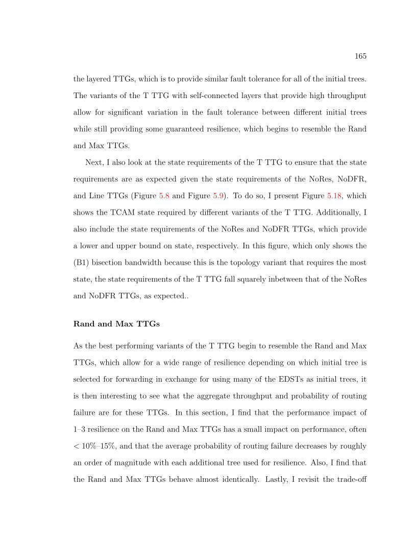
165
the layered TTGs, which is to provide similar fault tolerance for all of the initial trees.
The variants of the T TTG with self-connected layers that provide high throughput
allow for significant variation in the fault tolerance between different initial trees
while still providing some guaranteed resilience, which begins to resemble the Rand
and Max TTGs.
Next, I also look at the state requirements of the T TTG to ensure that the state
requirements are as expected given the state requirements of the NoRes, NoDFR,
and Line TTGs (Figure 5.8 and Figure 5.9). To do so, I present Figure 5.18, which
shows the TCAM state required by different variants of the T TTG. Additionally, I
also include the state requirements of the NoRes and NoDFR TTGs, which provide
a lower and upper bound on state, respectively. In this figure, which only shows the
(B1) bisection bandwidth because this is the topology variant that requires the most
state, the state requirements of the T TTG fall squarely inbetween that of the NoRes
and NoDFR TTGs, as expected..
Rand and Max TTGs
As the best performing variants of the T TTG begin to resemble the Rand and Max
TTGs, which allow for a wide range of resilience depending on which initial tree is
selected for forwarding in exchange for using many of the EDSTs as initial trees, it
is then interesting to see what the aggregate throughput and probability of routing
failure are for these TTGs. In this section, I find that the performance impact of
1–3 resilience on the Rand and Max TTGs has a small impact on performance, often
< 10%–15%, and that the average probability of routing failure decreases by roughly
an order of magnitude with each additional tree used for resilience. Also, I find that
the Rand and Max TTGs behave almost identically. Lastly, I revisit the trade-off

166
between size of the subset per destination and number of virtual channels used for
multipathing, showing that, surprisingly, variants of the Rand and Max TTGs with
either 12-trees per destination and 4-way multipathing behave almost identically to
using 8-trees per destination and 4-way multipathing, only with a slight increase in
fault tolerance. This result is particularly interesting for hybrid networks because
it implies that lossless forwarding does not need to use all of the available virtual
channels for performance so that the remaining virtual channels could be used for
lossless forwarding, if desired.
To start off, Figure 5.19 and Figure 5.20 show the throughput achieved by variants
of the Rand and Max TTGs with varying resilience (*-R), number of trees per des-
tination (T-*), degrees of multipathing (*-E), and sorting the initial trees either for
performance (P) or resilience (R) on variants of the Jellyfish and EGFT topologies,
respectively, with varying numbers of hosts and bisection bandwidths (B*). The first
thing that these figures show is that the throughput of both the Rand and Max TTGs
closely tracks that of deadlock-oblivious reactive shortest path routing (SP), especially
given no or relatively few failures. To some extent, this is expected. Because the 0-R
variants allow for all trees to be used as initial trees, these variants behave identically
to the NoRes TTG given no failures. Although increasing guaranteed resilience in
the other *-R variants disallows a number of trees from being initial trees equal to
the level of resilience, the impact of this on performance is also relatively small. For
example, given no failures on the (B1) 1024-host EGFT topology, the Rand 0-R TTG
reduced forwarding throughput by 6.5% when comapared with SP, while the Rand
3-R TTG only reduced forwarding throughput by 10.9%. While this impact increases
with topology size, the impact is still small, with the Rand 0-R TTG on a 2048-host
(B2) EGFT reducing forwarding throughput by 6.7%, the Rand 3-R TTG reducing

167
20 21 22 23 24 25 26 27 28
Number of Failures0.740.760.780.800.820.840.860.88
Norm
aliz
ed T
hrou
ghpu
t
SPMax 0-R (P)Rand 0-R (P)Rand 1-R (P)Rand 0-R (R)
Max 1-R (P)Max 0-R (R)Max 1-R (R)Rand 1-R (R)
Rand 2-R (P)Max 2-R (P)Max 2-R (R)Rand 2-R (R)
Max 3-R (P)Rand 3-R (P)Rand 3-R (R)Max 3-R (R)
(a) T-8 8-E 1024-hosts (B1)
20 21 22 23 24 25 26 27 28
Number of Failures0.740.760.780.800.820.840.860.88
Norm
aliz
ed T
hrou
ghpu
t
SPRand 0-R (P)Max 0-R (P)Max 1-R (P)Rand 1-R (P)
Rand 0-R (R)Max 0-R (R)Max 2-R (P)Rand 2-R (P)
Rand 1-R (R)Max 1-R (R)Rand 2-R (R)Rand 3-R (P)
Max 3-R (P)Max 2-R (R)Max 3-R (R)Rand 3-R (R)
(b) T-12 4-E 1024-hosts (B1)
210 211
Number of Hosts0.60
0.65
0.70
0.75
0.80
0.85
Norm
aliz
ed T
hrou
ghpu
t
SPRand 0-R (P)Max 0-R (P)Rand 0-R (R)Max 0-R (R)
Max 1-R (P)Rand 1-R (P)Max 1-R (R)Rand 1-R (R)
Max 2-R (P)Rand 2-R (P)Max 2-R (R)Rand 2-R (R)
Rand 3-R (P)Max 3-R (P)Rand 3-R (R)Max 3-R (R)
(c) T-8 8-E 16-F (B2)
210 211
Number of Hosts0.65
0.70
0.75
0.80
0.85
0.90
Norm
aliz
ed T
hrou
ghpu
t
SPRand 0-R (P)Max 0-R (P)Rand 0-R (R)Rand 1-R (P)
Max 0-R (R)Max 1-R (P)Rand 1-R (R)Max 1-R (R)
Max 2-R (P)Rand 2-R (P)Rand 2-R (R)Max 2-R (R)
Rand 3-R (P)Max 3-R (P)Max 3-R (R)Rand 3-R (R)
(d) T-12 4-E 16-F (B2)
210 211
Number of Hosts0.400.450.500.550.600.650.70
Norm
aliz
ed T
hrou
ghpu
t
SPRand 0-R (P)Max 0-R (P)Rand 1-R (P)Max 1-R (P)
Rand 0-R (R)Max 0-R (R)Rand 2-R (P)Max 2-R (P)
Rand 3-R (P)Rand 1-R (R)Rand 2-R (R)Max 2-R (R)
Max 1-R (R)Max 3-R (R)Max 3-R (P)Rand 3-R (R)
(e) T-8 8-E 16-F (B4)
210 211
Number of Hosts0.45
0.50
0.55
0.60
0.65
0.70
Norm
aliz
ed T
hrou
ghpu
t
SPRand 0-R (P)Max 0-R (P)Rand 1-R (P)Max 1-R (P)
Max 2-R (P)Rand 2-R (P)Max 3-R (P)Rand 0-R (R)
Rand 3-R (P)Max 2-R (R)Rand 1-R (R)Max 0-R (R)
Rand 2-R (R)Max 3-R (R)Max 1-R (R)Rand 3-R (R)
(f) T-12 4-E 16-F (B4)
Figure 5.19 : Jellyfish Throughput for the Rand and Max TTGs

168
20 21 22 23 24 25 26 27 28
Number of Failures0.450.500.550.600.650.700.750.80
Norm
aliz
ed T
hrou
ghpu
t
SPMax 0-R (P)Rand 0-R (P)Rand 1-R (P)Max 1-R (P)
Rand 0-R (R)Max 0-R (R)Rand 2-R (P)Rand 1-R (R)
Max 2-R (P)Max 1-R (R)Max 2-R (R)Rand 2-R (R)
Rand 3-R (P)Max 3-R (P)Max 3-R (R)Rand 3-R (R)
(a) T-8 8-E 1024-hosts (B1)
20 21 22 23 24 25 26 27 28
Number of Failures0.400.450.500.550.600.650.700.750.80
Norm
aliz
ed T
hrou
ghpu
t
SPMax 0-R (P)Rand 0-R (P)Max 1-R (P)Rand 1-R (P)
Max 2-R (P)Rand 2-R (P)Rand 0-R (R)Max 0-R (R)
Rand 1-R (R)Max 3-R (P)Rand 3-R (P)Max 1-R (R)
Rand 2-R (R)Max 2-R (R)Rand 3-R (R)Max 3-R (R)
(b) T-12 4-E 1024-hosts (B1)
210 211
Number of Hosts0.400.420.440.460.480.500.52
Norm
aliz
ed T
hrou
ghpu
t
SPRand 0-R (P)Max 0-R (P)Max 0-R (R)Rand 0-R (R)
Max 1-R (P)Rand 1-R (P)Max 1-R (R)Rand 1-R (R)
Rand 2-R (P)Max 2-R (P)Max 2-R (R)Rand 2-R (R)
Rand 3-R (P)Max 3-R (P)Max 3-R (R)Rand 3-R (R)
(c) T-8 8-E 16-F (B2)
210 211
Number of Hosts0.400.420.440.460.480.500.52
Norm
aliz
ed T
hrou
ghpu
t
SPMax 0-R (P)Rand 0-R (P)Max 0-R (R)Rand 0-R (R)
Rand 1-R (P)Max 1-R (P)Max 1-R (R)Rand 1-R (R)
Max 2-R (P)Rand 2-R (P)Max 2-R (R)Rand 2-R (R)
Rand 3-R (P)Max 3-R (P)Rand 3-R (R)Max 3-R (R)
(d) T-12 4-E 16-F (B2)
210 211
Number of Hosts0.260.280.300.320.340.360.380.40
Norm
aliz
ed T
hrou
ghpu
t
SPMax 0-R (P)Rand 0-R (P)Rand 0-R (R)Rand 1-R (P)
Max 1-R (P)Rand 2-R (P)Max 2-R (P)Max 0-R (R)
Max 1-R (R)Rand 1-R (R)Rand 3-R (P)Max 2-R (R)
Rand 2-R (R)Max 3-R (P)Rand 3-R (R)Max 3-R (R)
(e) T-8 8-E 16-F (B4)
Figure 5.20 : EGFT Throughput for the Rand and Max TTGs

169
throughput by 14.3%, and the other TTGs falling somewhere in-between.
These figures also show that neither the Rand or Max TTG dominates the other in
terms of performance, and, similarly, neither the “res” or “perf” ordering dominated
the other. Across the topologies considered in these figures, neither the Rand or Max
TTGs or the “res” or “perf” orderings had an obvious predictable improvement over
the other, even slight. Instead, the performance of the different variants were similar,
and the better performing variant differs across topology instances.
Further, these figures illustrate what is an interesting point in the trade-off be-
tween reducing either the number of virtual channels or the subset of the TTG in-
stalled for each destination to reducing forwarding table state. Surprisingly, the “T-8
8-E” and “T-12 4-E” TTG variants provide near-identical forwarding table through-
put across a range of number of failures, topologies, and bisection bandwidths. How-
ever, the “12-T 8-E” and “16-T 8-E” TTG variants, while not shown, had forwarding
throughput even closer to that of SP. This shows that, if more forwarding table state
or custom forwarding hardware can be dedicated to DF-EDST resilience, then the
impact of forwarding throughput can be even further reduced.
Given that the Rand and Max TTGs do not have a significant impact on forward-
ing, it is then worth asking how likely it is for routes in the Rand and Max TTGs to
experience a routing failure. To answer this questions, Figure 5.21 and Figure 5.22
show the average fault tolerance of different variants of the Rand and Max TTGs
on a range of Jellyfish and EGFT topologies, respectively. These figures show that
a 3-resilient Max TTG can reduce the probability of routing failure by about three
orders of magnitude when compared with non-resilient forwarding (NoRes). This is
an important result because I have previously shown that this TTG only reduces the
full load aggregate throughput of the network by about 5–10%. While only reducing

170
20 21 22 23 24 25 26 27 28
Number of Failures10-910-810-710-610-510-410-3
Frac
tion
ofFl
ows
Faile
d
NoRes 8-TRand 0-R (R)Rand 0-R (P)Max 0-R (P)Rand 1-R (P)
Rand 1-R (R)Max 0-R (R)Rand 2-R (P)Max 1-R (P)Max 1-R (R)
Rand 2-R (R)Max 2-R (P)Max 2-R (R)Rand 3-R (R)
Rand 3-R (P)Max 3-R (R)Max 3-R (P)NoDFR 8-T
(a) T-8 8-E 1024-hosts (B1)
20 21 22 23 24 25 26 27 28
Number of Failures10-910-810-710-610-510-410-3
Frac
tion
ofFl
ows
Faile
d
NoRes 8-TRand 0-R (P)Rand 0-R (R)Rand 1-R (P)Max 0-R (P)
Rand 1-R (R)Rand 2-R (R)Max 0-R (R)Rand 2-R (P)Max 1-R (P)
Max 2-R (P)Max 1-R (R)Rand 3-R (P)Rand 3-R (R)
Max 2-R (R)Max 3-R (P)Max 3-R (R)NoDFR 8-T
(b) T-12 4-E 1024-hosts (B1)
210 211
Number of Hosts10-9
10-8
10-7
10-6
10-5
10-4
Frac
tion
ofFl
ows
Faile
d
NoRes 8-TRand 0-R (P)Rand 0-R (R)Max 0-R (P)Max 0-R (R)
Rand 1-R (R)Rand 1-R (P)Max 1-R (R)Max 1-R (P)Rand 2-R (R)
Max 2-R (P)Rand 2-R (P)Max 2-R (R)Rand 3-R (R)
Max 3-R (P)Rand 3-R (P)Max 3-R (R)NoDFR 8-T
(c) T-8 8-E 16-F (B2)
210 211
Number of Hosts10-9
10-8
10-7
10-6
10-5
10-4
Frac
tion
ofFl
ows
Faile
d
NoRes 8-TRand 0-R (P)Rand 0-R (R)Max 0-R (P)Max 0-R (R)
Rand 1-R (P)Rand 1-R (R)Max 1-R (R)Max 1-R (P)Rand 2-R (R)
Rand 2-R (P)Max 2-R (R)Max 2-R (P)Rand 3-R (P)
Max 3-R (P)Max 3-R (R)NoDFR 8-TRand 3-R (R)
(d) T-12 4-E 16-F (B2)
210 211
Number of Hosts10-9
10-8
10-7
10-6
10-5
10-4
Frac
tion
ofFl
ows
Faile
d
NoRes 8-TRand 0-R (P)Rand 0-R (R)Max 0-R (P)Max 0-R (R)
Rand 1-R (P)Rand 1-R (R)Max 1-R (P)Max 1-R (R)Rand 2-R (P)
Max 2-R (P)Rand 2-R (R)Max 2-R (R)Rand 3-R (P)
Max 3-R (R)Max 3-R (P)Rand 3-R (R)NoDFR 8-T
(e) T-8 8-E 16-F (B4)
210 211
Number of Hosts10-9
10-8
10-7
10-6
10-5
10-4
Frac
tion
ofFl
ows
Faile
d
NoRes 8-TRand 0-R (P)Rand 0-R (R)Max 0-R (P)Max 0-R (R)
Rand 1-R (R)Rand 1-R (P)Max 1-R (R)Max 1-R (P)Rand 2-R (P)
Max 2-R (R)Max 2-R (P)Rand 2-R (R)Rand 3-R (P)
Max 3-R (R)Max 3-R (P)Rand 3-R (R)NoDFR 8-T
(f) T-12 4-E 16-F (B4)
Figure 5.21 : Probability of Routing Failure for the Rand and Max TTGs on the
Jellyfish Topology

171
20 21 22 23 24 25 26 27 28
Number of Failures10-910-810-710-610-510-410-3
Frac
tion
ofFl
ows
Faile
d
NoRes 8-TRand 0-R (R)Rand 0-R (P)Rand 1-R (R)Max 0-R (P)
Rand 1-R (P)Max 0-R (R)Max 1-R (R)Rand 2-R (R)Max 1-R (P)
Rand 2-R (P)Max 2-R (P)Rand 3-R (R)Max 2-R (R)
Rand 3-R (P)Max 3-R (P)Max 3-R (R)NoDFR 8-T
(a) T-8 8-E 1024-hosts (B1)
20 21 22 23 24 25 26 27 28
Number of Failures10-910-810-710-610-510-410-3
Frac
tion
ofFl
ows
Faile
d
NoRes 8-TRand 0-R (R)Rand 0-R (P)Rand 1-R (R)Max 0-R (P)
Rand 1-R (P)Max 0-R (R)Rand 2-R (R)Max 1-R (P)Rand 2-R (P)
Rand 3-R (P)Max 1-R (R)Max 2-R (P)Rand 3-R (R)
Max 2-R (R)Max 3-R (R)Max 3-R (P)NoDFR 8-T
(b) T-12 4-E 1024-hosts (B1)
210 211
Number of Hosts10-9
10-8
10-7
10-6
10-5
10-4
Frac
tion
ofFl
ows
Faile
d
NoRes 8-TRand 0-R (P)Rand 0-R (R)Max 0-R (R)Max 0-R (P)
Rand 1-R (R)Rand 1-R (P)Max 1-R (P)Max 1-R (R)Rand 2-R (P)
Rand 2-R (R)Max 2-R (R)Max 2-R (P)Max 3-R (P)
Rand 3-R (R)Rand 3-R (P)Max 3-R (R)NoDFR 8-T
(c) T-8 8-E 16-F (B2)
210 211
Number of Hosts10-9
10-8
10-7
10-6
10-5
10-4
Frac
tion
ofFl
ows
Faile
d
NoRes 8-TRand 0-R (R)Rand 0-R (P)Max 0-R (P)Max 0-R (R)
Rand 1-R (R)Rand 1-R (P)Max 1-R (R)Max 1-R (P)Max 2-R (P)
Rand 2-R (R)Rand 2-R (P)Max 2-R (R)Max 3-R (P)
Rand 3-R (P)Rand 3-R (R)Max 3-R (R)NoDFR 8-T
(d) T-12 4-E 16-F (B2)
210 211
Number of Hosts10-8
10-7
10-6
10-5
10-4
Frac
tion
ofFl
ows
Faile
d
NoRes 8-TRand 0-R (R)Rand 0-R (P)Max 0-R (P)Max 0-R (R)
Rand 1-R (P)Rand 1-R (R)Max 1-R (P)Max 1-R (R)Max 2-R (P)
Rand 2-R (P)Max 2-R (R)Rand 2-R (R)Max 3-R (P)
Max 3-R (R)Rand 3-R (R)Rand 3-R (P)NoDFR 8-T
(e) T-8 8-E 16-F (B4)
Figure 5.22 : Probability of Routing Failure for the Rand and Max TTGs on the
EGFT Topologies

172
throughput by 5–10% can reduce the probability of routing failure by as much as 4
orders of magnitude given 16 edges failures.
Additionally, these figures also show that even the 0-resilient variants of the Rand
and Max TTGs are more fault tolerant that the NoRes TTG. Across a wide range of
failures and topologies, the 0-resilient variants of the Rand and Max TTGs experience
roughly an order of magnitude fewer routing failures than the NoRes TTG on average.
This is important because, given 0 failures, the 0-resilient Rand and Max TTGs
behave identically to the NoRes TTG. However, the big difference is that the 0-
resilient Rand and Max TTGs use a TTG that allows for improved fault tolerance by
allowing packets to transition between initial trees, as long as the resultant TTG is
acyclic. While this does not guarantee even 1-resilience, as there will be at least one
tree initial tree that, if chosen, cannot transition to any other tree, the fact that this
improves fault tolerance is important because this implies that fault tolerance can
be improved when EDSTs are used for deadlock-freedom without further reducing
forwarding throughput.
However, unlike with throughput, which was nearly equal for the 8-T 8-T variants
and the 12-T 4-E variants, the 12-T 4-E variants are slightly more fault tolerant.
While is is expected, what is surprising is that the 8-T 8-E and 12-T 4-E variants
largely track each other in terms of average probability of routing failure. Because
I have already shown that multipathing does not impact fault tolerance, this lack
of a large difference in fault tolerance on most of variants the 8-T and 12-T TTGs
may not be expected. However, this is because not all initial trees in the Rand and
Max TTGs provide the same level of resilience. What has a larger impact on fault
tolerance than increasing the total number of trees is by increasing the number of
trees set aside for guaranteed resilience, and the number of set aside trees is equal in

173
the 8-T and 12-T variants with the same resilience.
Further, the results for the probability of routing failure are similar to that for
the variants of the T TTG that I evaluated. For example, given a 1024-host (B1)
EGFT topology and 64-failures, the T TTGs that I evaluated, which ranged from
2-resilient to 4-resilient, saw that, on average, a fraction of between 1.5e-5 and 4.2e-7
of the flows failed, with the best 3-resilient variant (T-8 5-ML0) having 6.9e-7 of the
flows fail (Figure 5.15). For a point of comparison, Figure 5.22b shows 0-resilient to
3-resilient variants of the Rand and Max TTGs given a 1024-host (B1) EGFT. Given
64 failures, this figure shows that these fraction of failed flows is in between 2.8e-5
and 1.3e-6. Although the best 3-resilient T TTG experiences fewer failures than the
best 3-resilient Rand or Max TTG, this is expected. In the 3-resilient Rand and Max
TTGs, only 3 out of the total of 20 EDSTs on this topology are reserved for resilience
and are not used as initial trees. On the other hand, 12 out of the 20 EDSTs in the
best performing 3-resilient TTG are reserved for fault tolerance. While the forwarding
function is only 3-resilient per destination in the end, having more trees to choose
between allows for trees with shortest paths to be chosen, and trees with shorter path
lengths are less likely to encounter a failed link because they encounter fewer total
links. However, as expected, while decreasing the number of initial trees improves
fault tolerance, doing so also has a more noticeable impact on fault tolerance.
Lastly, these figures also show that, as with aggregate throughput, neither the
Rand nor Max TTG dominates the other and neither the “perf” or “res” sorting
dominates the other.
Next, I evaluated the state requirements of different variants of the Rand and Max
TTGs, which are presented in Figure 5.23. While this figure covers both the EGFT
and Jellyfish topologies and (B1) and (B4) variants, the results may be summarized
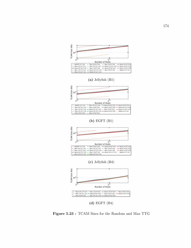
174
210 211
Number of Hosts
104
TCAM
Siz
e (K
b)
NoDFR 12-T 4-EMax 0-R 12-T 4-ERand 0-R 12-T 4-EMax 1-R 12-T 4-EMax 2-R 12-T 4-E
Max 0-R 8-T 8-EMax 3-R 12-T 4-EMax 1-R 8-T 8-ERand 2-R 12-T 4-ERand 3-R 12-T 4-E
Max 2-R 8-T 8-ERand 1-R 12-T 4-ERand 0-R 8-T 8-EMax 3-R 8-T 8-E
Rand 2-R 8-T 8-ERand 3-R 8-T 8-ERand 1-R 8-T 8-ENoRes 12-T 4-E
(a) Jellyfish (B1)
210 211
Number of Hosts
104
TCAM
Siz
e (K
b)
NoDFR 12-T 4-EMax 0-R 12-T 4-EMax 1-R 12-T 4-EMax 2-R 12-T 4-EMax 0-R 8-T 8-E
Max 3-R 12-T 4-EMax 1-R 8-T 8-ERand 2-R 12-T 4-ERand 3-R 12-T 4-EMax 2-R 8-T 8-E
Rand 0-R 8-T 8-ERand 1-R 8-T 8-EMax 3-R 8-T 8-ERand 2-R 8-T 8-E
Rand 3-R 8-T 8-ERand 0-R 12-T 4-ERand 1-R 12-T 4-ENoRes 12-T 4-E
(b) EGFT (B1)
210 211
Number of Hosts
104
TCAM
Siz
e (K
b)
NoDFR 12-T 4-EMax 0-R 12-T 4-EMax 1-R 12-T 4-ERand 0-R 12-T 4-EMax 2-R 12-T 4-E
Max 0-R 8-T 8-EMax 3-R 12-T 4-ERand 1-R 12-T 4-EMax 1-R 8-T 8-ERand 2-R 12-T 4-E
Rand 0-R 8-T 8-EMax 2-R 8-T 8-EMax 3-R 8-T 8-ERand 3-R 12-T 4-E
Rand 2-R 8-T 8-ERand 3-R 8-T 8-ERand 1-R 8-T 8-ENoRes 12-T 4-E
(c) Jellyfish (B4)
210 211
Number of Hosts
104
TCAM
Siz
e (K
b)
Max 0-R 12-T 4-EMax 1-R 12-T 4-EMax 0-R 8-T 8-E
Max 1-R 8-T 8-ERand 0-R 8-T 8-EMax 3-R 12-T 4-E
Rand 1-R 8-T 8-EMax 2-R 8-T 8-ERand 2-R 8-T 8-E
Max 3-R 8-T 8-ERand 3-R 8-T 8-E
(d) EGFT (B4)
Figure 5.23 : TCAM Sizes for the Random and Max TTG

175
simply. All of the evaluated variants of the Rand and Max TTGs required nearly
the same amount of forwarding table state for a given topology, size, and bisection
bandwidth, including both Rand and Max TTGs and the “12-T 4-E” and “8-T 8-E”
variants. Additionally, the state required by these TTGs falls right in-between the
NoRes and NoDFR TTGs, which should be expected because the Max TTG should
have exactly half the number of edges as the NoDFR TTG. Similarly, the Rand TTG
should have roughly half the edges as the NoDFR TTG.
Although initially surprising, the nearly identical state requirements of all of the
variants helps shed some light on their similar throughput and probability of routing
failure. All things combined, all of these variants lead to about the same total num-
ber of trees and tree transitions, which is evident by their similar state. As with the
NoDFR and NoRes TTGs, it appears to not be of much significance how the trees are
ordered or derived. As long as the TTG is well connected, then the forwarding func-
tion can provide both high aggregate throughput and can be far more fault tolerant
than non-resilient forwarding.
Finally, all of the state requirements in this section assume that packets may be
marked with the current forwarding tree. If packets may not be modified, then the
state requirements of DF-EDST resilience should increase proportional to the average
degree of the EDSTs. To illustrate this increase in state, Figure 5.24 presents the
state requirements of the Rand and Max TTGs if packets are not modified at all.
This figure shows that both the EGFT and Jellyfish topologies require more 40Mbit
of TCAM state for topologies with (B1) topologies with 2K hosts. Further, I found
that the (B2) and (B4) topologies required more than 40Mbit of TCAM state for
topologies with 3K hosts.

176
210 211
Number of Hosts
104
TCAM
Siz
e (K
b)
Max 0-R 12-T 4-EMax 2-R 12-T 4-EMax 1-R 12-T 4-ERand 0-R 12-T 4-EMax 0-R 8-T 8-E
Max 3-R 12-T 4-ERand 2-R 12-T 4-EMax 1-R 8-T 8-ERand 3-R 12-T 4-EMax 2-R 8-T 8-E
Max 3-R 8-T 8-ERand 1-R 12-T 4-ERand 0-R 8-T 8-ERand 3-R 8-T 8-E
Rand 2-R 8-T 8-ERand 1-R 8-T 8-ENoRes 12-T 4-ENoDFR 12-T 4-E
(a) Jellyfish (B1)
210 211
Number of Hosts
104
TCAM
Siz
e (K
b)
Max 0-R 12-T 4-EMax 1-R 12-T 4-EMax 3-R 12-T 4-EMax 2-R 12-T 4-ERand 3-R 12-T 4-E
Rand 2-R 12-T 4-EMax 1-R 8-T 8-EMax 2-R 8-T 8-EMax 0-R 8-T 8-EMax 3-R 8-T 8-E
Rand 0-R 12-T 4-ERand 2-R 8-T 8-ERand 3-R 8-T 8-ERand 1-R 12-T 4-E
Rand 1-R 8-T 8-ERand 0-R 8-T 8-ENoRes 12-T 4-ENoDFR 12-T 4-E
(b) EGFT (B1)
Figure 5.24 : TCAM Sizes for the Random and Max TTG if packets are not labeled

177
Overall TTG Comparison
Given that Section 5.4.2 shows that some of the variants of the layered TTGs provide
2–4-resilience with only a small impact on performance and that Section 5.4.2 shows
the same for the Rand and Max TTGs, this raises an obvious question. Which of the
TTG variants is the best? To answer this question, I would compare the best variants
of the T, ALayer, MLayer, Rand, and Max TTGs with either the “perf” or “res”
layer orderings for a range of different degrees of multipathing and number of trees
per-destination, deciding an ultimate winner that provides the best fault tolerance
within a set percent impact on forwarding throughput, for a range of forwarding
throughputs. However, instead of answering this question, I ask a different question.
Are the best variants of the T TTGs, the Rand TTG, and the Max TTG given either
of the two different layer orderings even that different from each other? Ultimately,
I conclude no, which implies that the results in Section 5.4.2 already illustrate the
complete trade-off between resilience and fault tolerance, showing that, at best, extra
fault tolerance can be provided without any impact on performance, and, at a small
extra impact to performance, often < 5%, 2–4 more failures are guaranteed to be
tolerated and the average likelihood of a routing failure can be reduced by 2–4 orders
of magnitude.
The reason for this conclusion is because the T TTG clearly dominates the ALayer
or MLayer TTGs, and the best performing variant of the T TTG uses a self-connected
layer-0. In this case, this TTG is essentially the same as the Max TTG. Both have
initial trees that are connected in a line, and then remaining trees in both TTGs
are themselves arranged into a line for resilience. Further, the Rand TTG leads to a
TTG where all of the initial trees are highly connected, which is also quite similar.

178
Similarly, the “perf” and “res” sortings do not lead to subsets of the TTG that would
be expected to behave that differently. The trees are sorted according to shortest
average path length across all destinations before assigning then to nodes in the
TTG, so these orderings may be the same for some destinations.
5.5 Discussion
The result that the “12-T 4-E” variants of the Rand and Max TTGs match the
performance of “8-T 8-E” variants, in addition to showing that DF-EDST resilience
is flexible, has an useful implication. If the 4-E variant is used, then not all of the
virtual channels need to be dedicated just to lossless forwarding. Instead, lossless
forwarding of varying levels of QOS can use the other half of the available virtual
channels in any of a number of ways [62, 34]. In this case, the performance impact
of lossless forwarding is even less important as lossy background flows can consume
all of the remaining bandwidth.
Further, because this shows that not all virtual channels need to be used, on tree
topologies, fault tolerance can be provided without impacting default performance
at all if all default traffic uses minimal routing or, even further, just uses routing
that first travels up the tree then down. If all of the default traffic is forwarded on
its own, virtual channel, then it is still deadlock-free, and if a packet encounters a
failure, it may then transition between virtual channels and follow DF-EDST resilience
and, again, still be deadlock-free. In this case, the only drawback to providing fault
tolerance is forwarding table state.
Although the results of Section 5.4.1 that DF-FI resilience is not a scalable solution
to providing both fault tolerance and deadlock-free routing, they do show that naively
using minimal routing and enabling lossless forwarding with reactive fault tolerance,

179
similar to many of today’s networks 0-resilient, does in fact fit within the number of
available virtual channels, even on topologies that are not trees. This implies that
even if it is not acceptable to restrict routing, as in instead using the NoRes TGG,
then it should be possible to enable lossless forwarding on today’s networks, which
already support DCB.
At initial consideration, my result that a line TTG can be used to improve up
the result from Feigenbaum et al., showing that there always exists a max(1, k/2−1)
forwarding pattern that does not modify packets may not seem practical as it provides
poor forwarding throughput when implemented for deadlock-free routing as all initial
forwarding paths use the same tree, a la Ethernet with RSTP. However, even in
deadlock-free routing, this implies that important and mission critical data may have
fault tolerance that is equal to the length of the longest line in the TTG minus one,
regardless of the fault tolerance that is provided for other traffic. Moreover, this result
also has further implications given non-deadlock-free routing, where each destination
may use a different TTG. Although default trees may not be used in this case because
the forwarding function needs to be able to uniquely map the input port to the current
forwarding tree, the initial forwarding tree(s) for each destination may be chosen to
be the shortest of the EDSTs for the destination. This implies that existing networks
where introducing new packet formats is not allowed but that still allow for fault
tolerant forwarding, such as IP-FRR [63] and, arguably, OpenFlow [64], can build a
forwarding function that is (k/2− 1)-resilient.
Given that Theorem 5.2.4 uses EDSTs to improve up the main result of Feigen-
baum et al. (Theorem 2.3.1), it is tempting to try to use ADSTs to further improve
upon this result. Just as with EDST resilience, if, for each destination, ADST re-
silience uses a line TTG, then 1) there exists a total ordering of channels for each

180
destination, so the forwarding function is acyclic even without marking tree failures
in packet headers and 2) input ports can still be used to identify the current ADST
if default trees are not used, so the current tree does not also need to be marked in
packet headers. However, this forwarding model presents one large problem for im-
proving upon Theorem 5.2.4. The proof that ADSTs can be used to protect against
up k−1 failures relies on the property that the tree that is chosen after an arc failure
must be the tree that uses the opposite arc of the failed arc, but this tree ordering
may be different for each switch and set of failures. While I use a routing algorithm
that respects this ordering in Chapter 4, doing so requires marking failed trees in a
packet header. Given a line TTG, this ordering may not be respected. Thus, such a
forwarding function is not guaranteed to be (k− 1)-resilient. Although the resilience
of such a forwarding function may be in fact greater than k/2 − 1, it is currently
unclear what the resilience of such a forwarding function would be given an arbitrary
topology. However, in the worst case, there may exist a topology such that regardless
of the tree ordering, there exists a source and destination and set of failures such
that the reverse tree ordering is never respected. In this case, only as many as half
of the trees may not be useful for providing resilience because there are only two
arcs per edge, so, even in this worse case, ADSTs should be at least able to provide
(k/2 − 1)-resilience. Thus, such an ADST forwarding model should at least be able
to match the resilience of a comparable EDST forwarding model. Further, such a
scenario would most likely be rare, so the expected fault tolerance could be improved
over that of EDSTs.
However, this discussion about using ADSTs to improve upon the result of Feigen-
baum et al. has further implications. Could ADSTs also be used to provide both
deadlock-free and fault tolerant routing? Just as with EDSTs, if the same set of

181
ADSTs is used for every destination, and the allowed transitions between trees are
acyclic, then the forwarding function of the network would be deadlock-free because
there exists a total ordering of all of the channels in the network. However, this solu-
tion is not without its problems. Unlike EDSTs, every ADST is directed on rooted at
a destination, so a path is not guaranteed not exist for every source and destination
on each ADST. Given that the existing algorithm for computing ADSTs [44] ensures
that each ADST is rooted at the same destination, this will likely lead to poor con-
nectivity and performance for some destinations, although, if an algorithm is used
that builds ADSTs that are rooted at either random or strategic locals, then it may
be possible to improve connectivity on highly connected data center topologies. How-
ever, because all switches must use the same subset of the TTG for each destination
to provide fault tolerance, there may still not be enough ADSTs that contain a route
from all or enough sources to a given destination. Although this is an interesting
approach to providing deadlock freedom and fault tolerance, I leave an evaluation of
this to future work.
5.6 Summary
In summary, I have introduced and evaluated two different approaches to implement-
ing both deadlock-free and fault-tolerant forwarding for data center networks, DF-FI
resilience and DF-EDST resilience. Despite introducing a new algorithm for assign-
ing paths to virtual channels, FAS-VC, I found that 1) FAS-VC does not find better
assignments than an existing virtual channel assignment algorithm and 2) DF-FI re-
quires far more virtual channels than are currently available to implement resilient
forwarding on data center topologies with 2048-hosts or more. Until further advances
are made on the topic of guaranteeing that some configurations of backup routes are

182
never possible and thus could never form deadlocks, DF-FI resilience is not entirely
practical.
However, this result also further motivates DF-EDST resilience. To enable DF-
EDST resilience, I first prove that DF-EDST resilience is deadlock-free as long as the
TTG is acyclic. This result itself is interesting as it is the first to improve upon the
main result from Feigenbaum et al. [30], showing that there always exists a max(1,
k/2 − 1)-resilient forwarding function that does not modify packet headers given
any aribtrary topology. Further, I also discuss the fault tolerance properties that is
implication that DF-EDST requires acyclic TTGs requires, including noting that the
resilience of the forwarding function is equal to the shortest height of any of the initial
trees minus one. However, this introduces a clear trade-off between performance and
resilience.
Given this trade-off, I then evaluated the aggregate throughput, average prob-
ability of routing failure, and forwarding table state requirements of a number of
different TTGs. I show that, with DF-EDST resilience, fault tolerant forwarding can
be provided on any arbitrary well-connected data center topology without impacting
throughput beyond that of existing approach to using EDSTs to provide deadlock-
free routing for lossless forwarding. In effect, the only extra cost of fault tolerance is
additional forwarding table state. Moreover, if even three of the total EDSTs in the
topology, of which there are often 10–20, are reserved for fault tolerance and guar-
anteed resilience (3-resilience), then the probability of routing failure can be reduced
by 3–4 orders of magnitude with only minimal impact on forwarding throughput
(5–10%).
Additionally, I also show that not all of the virtual channels are needed to provide
high throughput forwarding. This is important because all of the aforementioned
183
results apply to any arbitrary data center topologies, including the Jellyfish [47] and
HyperX [65]. If a data center network instead uses a tree topology, then it is possible
to do even better. If a single virtual channel is set aside, then all of the minimal
paths in the entire topology may be installed and any arbitrary traffic engineering
scheme may be used to balance the default traffic across these paths, a la XPath [53],
and the resultant forwarding function is still guaranteed to be deadlock-free. Further,
when this default traffic encounters a failure, it may transition to another virtual
channel that uses DF-EDST to build backup routes, and the forwarding function is
still guaranteed to be deadlock-free. In effect, the only limits on resilience even given
lossless forwarding on a tree topology are forwarding table state and the connectivity
of the underlying topology. The performance of traffic that does not encounter failures
should not be harmed.
Lastly, even though tree resilience requires 40Mbit of TCAM state to implement
DF-EDST with 12-trees per destination and 4-way multipathing on a 1 : 1 bisection
bandwidth ratio Jellyfish topology with about 3K hosts and a 1 : 1 bisection band-
width ratio EGFT topology with about 5K hosts, I do not consider these forwarding
table state requirements to be limiting. First off, given a 1 : 1 bisection bandwidth
ratio, these topologies are still fairly large for flat layer-2 networks. Additionally,
DF-EDST resilience requires far less forwarding table state as bisection bandwidth
is reduced. I would expect DF-EDST resilience to scale to 1 : 4 bisection bandwidth
networks with close to 10K hosts. Further, because of the clear trade-off between
fault tolerance and forwarding table state, these state requirements do not imply to
DF-EDST resilience is not possible given larger topologies. Instead, only fault tol-
erance needs to be reduced, which is an especially reasonable compromise if there
are multiple classes of traffic in the network. Lastly, these results just further moti-

184
vate building switches with forwarding table hardware specifically designed for tree
resilience. I believe that, given a custom implementation, the forwarding table state
requirements of the resilient TTGs could be reduced to match that of using EDSTs
for non-fault-tolerant but deadlock-free forwarding.

185
CHAPTER 6
Related Work
In this section, I discuss related work in more detail. For the sake of discussion, I first
discuss related work on congestion control and then I discuss related work on fault
tolerant routing.
6.1 Congestion Control and Avoidance
My discussion of related work focuses on efforts to reduce flow completion times in
the data center.
Like TCP-Bolt, zOVN [40] observes that enabling DCB can reduce flow completion
times. However, their primary focus is enabling DCB support in vSwitches. Further,
they use standard TCP variants, which I have shown can perform poorly, and they
do not explore the possibility of disabling slow start.
Also like my work, DeTail [9] reduces the tail of flow completion times in data
centers with a new network stack that uses DCB and packet spraying to balance
network load. However, unlike my work, DeTail continues to use the default TCP
initial congestion window on top of DCB and does not address deadlock free routing.
Complementary to my work are transport protocols that introduce mechanisms to
prioritize traffic [39, 66, 67, 68]. These protocols approach reducing flow completion
times by applying either a shortest-flow-first, an earliest-deadline-first, or a least-

186
attained-service schedule.
Remy [69], a new TCP variant, uses machine learning to design TCP congestion
control algorithms. I expect that extending Remy to support ECN could automati-
cally generate a congestion control algorithm that outperforms DCTCP, which would
improve the performance of TCP-Bolt.
Two other recent proposals for achieving faster flow completion times are notable:
TDMA in the data center [70] and HULL [33]. The former uses the pause-frame
primitive to implement a TDMA packet schedule for low latency [70]. However, as
the authors acknowledge, it is unclear whether an effective centralized controller can
be built to handle arbitrary topologies and workloads. HULL [33] reduces latency at
the cost of total network throughput but does not attempt to improve overall flow
completion times.
While this thesis uses virtual lanes to enable or improve DFR, RC3 [71] introduces
another use for the virtual lanes provided by DCB. In RC3, virtual lanes are assigned
to different priorities and are used to safely start transmitting at line rate. While this
is also a property provided by TCP-Bolt, RC3 uses a different mechanism to avoid
congestion failure. Rather than relying on DCB to avoid dropping packets, RC3
follows normal TCP slow-start dynamics on the highest priority queues and achieves
line-rate transmissions by speculatively sending traffic on the lower priority queues.
In the case of congestion, the lower priority speculative traffic should be dropped
first, so TCP performance should never be any worse than without RC3. While it is
unclear exactly how RC3 performance compares with TCP-Bolt, RC3, unlike TCP-
Bolt, does not solve the incast problem and can drop packets after they have already
consumed otherwise usable bandwidth upstream in the network.

187
6.2 Fault Tolerant Forwarding
While I have mainly discussed MPLS-FRR, FCP, and the work of Feigenbaum et
al. [30] that formalized resilience, there is other significant work on resilience. Due to
the extent of the approaches to resilience and forwarding table compression, I limit
my discussion to a few closely related projects.
XPath [53] introduces a new forwarding table compression algorithm so as to allow
for all desired paths to be preinstalled in a network. XPath’s algorithm operates
by first grouping paths into path sets, then it assigns labels to path sets so that,
considering all forwarding tables, entries that share outputs at switches have labels
that share prefixes so they can be compressed. Because MPLS-FRR and FCP have
assignable labels, XPath can compress them, subject to the previously discussed
lower bound. Because Plinko uses a path instead of a label, XPath is not applicable
to Plinko.
Next, I have yet to consider some related work on routing failures for a variety for
reasons. For example, ECMP, IP Fast Re-route [63], and Fat Tire [72] offer limited
resilience. Packet re-cycling [73] and Borokhovich et al. [74] use inefficient paths.
R-BGP [75] and F10 [60] rely on graph-specific properties. DDC [76] guarantees
connectivity but at least temporarily incurs significant stretch and can suffer from
forwarding loops, although an IP TTL may terminate the forwarding of a packet, and
KF [77] also allows loops.
Packet Re-cycling (PR) [73] introduces a new algorithm for pre-computing for-
warding tables that are fully resilient and only require and additional log2(|D|) bits
of data in a packet’s headers. However, PR cannot use arbitrary paths, and path
lengths in PR are typically far from minimal in the presence of failures, unlike the

188
discussed forwarding models. This is because PR routes around failures in a manner
akin to solving a labyrinth by the right-hand rule.
DDC [76], or data-driven connectivity, provably provides ideal forwarding-
connectivity, which only guarantees that a packet will reach its destination as
long as the network remains physically connected. DDC achieves ideal forwarding-
connectivity by performing provably safe link-reversals in response to incorrect for-
warding. If the forwarding function initial forms a DAG, then reversing the direction
of all of a switch’s links in the forwarding function at once is guaranteed to produce
another DAG. DDC repeats link-reversal operations until the forwarding DAG con-
verges to a “destination-oriented” DAG, which, for n switches, is guaranteed to occur
after O(n2) reversal operations.
The key differences between DDC and the evaluated forwarding models are that
DDC can temporarily incur significant stretch, and, in DDC, packets on the side
of a partition that is not connected to the packet’s destination will persistently be
forwarded in loops until either the control plane detects the partition and deletes
routes, a TTL in the packet, if any, expires, or the packet is dropped due to congestion.
In contrast, the models evaluated in this thesis all guarantee that packets will be
dropped in the event of a partition.
Although these projects do not meet my goal of implementing efficient OpenFlow
fast failover, they can be complementary. For example, DDC [76], or data-driven
connectivity, is a complementary project. On one hand, DDC can temporarily incur
significant stretch, and, in the case of a partition, packets will be looped until a TTL
expires, so Plinko is preferable for routing failures it can prevent. On the other hand,
DDC will always converge to a route given the destination is not partitioned, so if
Plinko experiences a routing failure, it may be desirable to fall back on DDC for

189
important traffic.
Keep Forwarding (KF) [77] also works towards building t-resilient forwarding ta-
bles. However, KF, also does not build routes that meet the definition of resilience
because it does not guarantee loop freedom, even when the destination is not discon-
nected from the source. Like DDC, KF relies of TTL fields, which is not suitable for
Ethernet and can lead to periods of congestion failure in IP networks.
Lastly, DF-EDST resilience can be thought of as a new variant of Up*/Down*
routing [21, 18] for well connected topologies. While Up*/Down* builds a single tree
and assigns directions to all links based on this tree, DF-EDST builds multiple trees
and assigns directions to links based on the tree they are a member of. If only a
single EDST exists, then Up*/Down* should perform better than DF-EDST because
Up*/Down* allows for all of the links in the network, even ones that are not a member
of an EDST. However, on highly connected data center topologies, Up*/Down* leads
to highly restricted routing when compared with DF-EDST.

190
CHAPTER 7
Conclusions
Given both the size of today’s data center networks and the bursty traffic patterns of
many data center applications, at any point in time there is likely to be packet loss due
to some kind of network failure. In this thesis, I present new approaches to handling
common and disrupting network failures, improving the performance of the network.
Specifically, this thesis focuses on simultaneously addressing the two most common
kinds of failures in data center networks: congestion failures and routing failures.
To handle congestion failures, this thesis introduces TCP-Bolt, which utilizes DCB
to reduce flow completion times. To handle routing failures, this thesis introduces
Plinko, a new forwarding model for local fast failover that provides better performance
and requires less forwarding table state than EDST resilience. Unfortunately, enabling
DCB for TCP-Bolt makes a new kind of failure, deadlock, possible. To enable the use
of DCB with local fast failover, this thesis introduces the first ever approaches to local
fast failover that guarantee deadlock-free routing for arbitrary network topologies,
deadlock-free Plinko (DF-FI resilience) and DF-EDST resilience.
Specifically, TCP-Bolt combines DCB with data center congestion control with
bandwidth-delay product sized initial congestion windows to achieve shorter flow
completion times. Three aspects of TCP-Bolt are demonstrated in the course of
this thesis: I show the existence of fairness, head-of-line blocking, and bufferbloat
191
problems with DCB on real network hardware. I show that, despite the associated
pitfalls, it is practical to enable DCB in a fully converged network because of TCP-
Bolt. Lastly, I show that doing so provides flow completion time benefits. Using
DCB and disabling TCP’s conservative initial congestion window on an uncongested
network can reduce flow completion times by 50 to 70%. Under a realistic workload,
TCP-Bolt reduces flow completion times by up to 90% compared to DCTCP for
medium flow sizes, while simultaneously matching the performance of DCTCP for
short, latency-sensitive flows.
To solve routing failures, this thesis explores the feasibility of implementing local
fast failover groups in hardware, even though prior work assumes that state explosion
would limit hardware resilience to all but the smallest networks or uninteresting lev-
els of resilience [25]. Specifically, this thesis presents a number of practical advances
that increase the applicability of hardware resilience. First, I have introduced a new
forwarding table compression algorithm. Because forwarding table compression is
limited by the number of unique (output, action) pairs in the table, I also introduced
two ways to lower this bound. In order to increase the number of common output
paths in a forwarding table, I introduce the concept of compression-aware routing,
and I find that it is highly effective when combined with my compression algorithm,
achieving compression ratios ranging from 2.22× to 19.77× given 4-resilient routes
on Jellyfish topologies. In order to reduce the number of unique actions, which lim-
its compression in both MPLS-FRR and FCP, I introduce Plinko, a new forwarding
model that applies the same action to every packet. Everything combined, I expect
that 4-resilient and 6-resilient Plinko will easily scale to networks with tens of thou-
sands of hosts. In contrast, I expect that fully optimized FCP, MPLS-FRR, and
ADST and EDST resilience could provide 4-resilience for topologies with 8192 hosts.

192
However, solving congestion failures with TCP-Bolt is not orthogonal from local
fast failover, as DCB requires that all routes, including backup routes, must be dead-
lock free. Although it would be desirable to enable both TCP-Bolt and Plinko, doing
so could lead to deadlock, which can render the entire network unable to forward
traffic. Because of this, Plinko and the other deadlock-oblivious local fast failover
schemes considered in this thesis should only be used on networks whose operators
are unwilling to enable DCB. Instead, local fast failover should be provided by ei-
ther one of two deadlock-free approaches to local fast failover on arbitrary network
topologies introduced in this thesis because doing so allows local fast failover to be
combined with TCP-Bolt.
Specifically, this thesis introduces and evaluates two different approaches to im-
plementing both deadlock-free and fault-tolerant forwarding for arbitrary data cen-
ter networks, DF-FI resilience and DF-EDST resilience. First, I find that DF-FI
resilience, which includes deadlock-free Plinko, is more desirable than DF-EDST re-
silience because of higher aggregate forwarding throughput and lower forwarding table
state requirements. However, DF-FI resilience is not applicable to all networks. DF-
FI resilience requires more virtual channels than are currently available in DCB to
implement resilient forwarding on data center topologies with more than 2K hosts.
Until further advances are made on the topic of guaranteeing that some configura-
tions of backup routes are never possible and thus could never form deadlocks, DF-FI
resilience is not a scalable solution.
However, this result also further motivates DF-EDST resilience, which this the-
sis proves is deadlock-free. With DF-EDST resilience, fault tolerant forwarding can
be provided on any arbitrary well-connected data center topology without impacting
throughput beyond that of using EDSTs to provide deadlock-free routing. In effect,

193
the only extra cost of fault tolerance is additional forwarding table state. Moreover,
if even three of the total EDSTs in the topology, of which there are often 10–20, are
reserved for fault tolerance and guaranteed resilience (3-resilience), then the proba-
bility of routing failure can be reduced by 3–4 orders of magnitude with only a small
impact on forwarding throughput. Although DF-FI is more desirable, these results
on DF-EDST resilience imply that high performance, fault tolerant, deadlock-free
routing is still possible on networks larger than the networks DF-FI resilience can be
implemented on.
In summary, with the addition of both new ways of using existing hardware mech-
anisms and the proposal of new hardware mechanisms, I show that the ways in which
data center networks handle failures can be made significantly more effective while
still operating fast enough and efficiently enough so as to avoid impacting perfor-
mance. Ultimately, this means that it is possible to significantly improve both flow
completion times and fault tolerance.
7.1 Future Work
I see three main avenues for future work to improve upon the research in this thesis.
The first is to reduce the state requirements of FCP. The second is to increase the
scalability of DF-FI resilience. The third is to increase the path diversity of DF-EDST
resilience.
Unlike Plinko, the compressibility of FCP routes is limited by the number of
unique output actions in the forwarding table. However, it may be possible to reduce
this limit by modifying the FCP routing algorithm. If packets are tagged with an ID
that represents a superset of the failures that a packet has encountered, then more
forwarding table entries could share a common action, improving compressibility.

194
However, it is unclear that such a forwarding function would be more compressible
than Plinko routes.
The primary factor that limits the scalability of DF-FI resilience is the number
of virtual channels that it requires. There are two ways in which the scalability of
DF-FI resilience could be improved. The first way is to design a new switch that
supports more virtual channels. The second approach is to reduce the number of
virtual channels required by DF-FI resilience. This could be done by improving the
virtual channel assignment algorithm. However, some configurations of backup routes
are never possible and thus could never form deadlocks. If this could be used to allow
for cycles in the channel dependency graph, then the virtual channel requirements of
DF-FI resilience could also be reduced.
Lastly, it may be possible to increase the path diversity of the routes in DF-EDST
resilience. Routing on edge disjoint spanning trees is sufficient but not necessary to
provide deadlock-free routing. On some topologies, such as oversubscribed topologies,
it may be possible that edges can be allowed to be shared between some trees so as to
increase the total number of trees. While this would not increase resilience, it could
increase average fault tolerance and path diversity. However, this approach is only
possible if it can be proven that the resulting forwarding function still leads to a total
ordering of channel requests.
195
Bibliography
[1] “Microsoft datacenters.” http://www.microsoft.com/en-us/server-cloud/
cloud-os/global-datacenters.aspx.
[2] “Facebook’s top open data problems.” https://research.facebook.com/
blog/1522692927972019/facebook-s-top-open-data-problems/.
[3] “My data is bigger than your data.” http://lintool.github.io/
my-data-is-bigger-than-your-data/.
[4] A. Roy, H. Zeng, J. Bagga, G. Porter, and A. C. Snoeren, “Inside the social
network’s (datacenter) network,” in SIGCOMM, 2015.
[5] P. Gill, N. Jain, and N. Nagappan, “Understanding network failures in data
centers: measurement, analysis, and implications,” in SIGCOMM, 2011.
[6] M. Alizadeh, A. Greenberg, D. A. Maltz, J. Padhye, P. Patel, B. Prabhakar,
S. Sengupta, and M. Sridharan, “DCTCP: Efficient packet transport for the
commoditized data center,” in SIGCOMM, 2010.
[7] Y. Chen, R. Griffith, J. Liu, A. D. Joseph, and R. H. Katz, “Understanding TCP
Incast Throughput Collapse in Datacenter Networks,” in SIGCOMM, Aug. 2009.
[8] V. Jacobson, “Congestion avoidance and control,” in SIGCOMM, ACM, 1988.
[9] D. Zats, T. Das, P. Mohan, D. Borthakur, and R. H. Katz, “DeTail: Reducing the
flow completion time tail in datacenter networks,” tech. rep., EECS Department,
University of California, Berkeley, 2012.

196
[10] W. J. Dally and C. L. Seitz, “Deadlock-free message routing in multiprocessor
interconnection networks,” IEEE Transactions on Computers, vol. C-36, pp. 547–
553, May 1987.
[11] M. Al-Fares, A. Loukissas, and A. Vahdat, “A scalable, commodity data center
network architecture,” SIGCOMM, 2008.
[12] D. Nagle, D. Serenyi, and A. Matthews, “The Panasas ActiveScale Storage Clus-
ter: Delivering scalable high bandwidth storage,” in SC ’04: Proceedings of the
2004 ACM/IEEE Conference on Supercomputing, (Washington, DC, USA), 2004.
[13] K. Ramakrishnan, S. Floyd, and D. Black, “The Addition of Explicit Congestion
Notification (ECN) to IP.” RFC 3168, Sept. 2001.
[14] S. Floyd and V. Jacobson, “Random early detection gateways for congestion
avoidance,” IEEE/ACM Trans. Netw., vol. 1, Aug. 1993.
[15] M. Alizadeh, S. Yang, S. Katti, N. McKeown, B. Prabhakar, and S. Schenker,
“Deconstructing datacenter packet transport,” HotNets, 2012.
[16] P. Prakash, A. Dixit, Y. Hu, and R. Kompella, “The TCP outcast problem:
exposing unfairness in data center networks,” NSDI, 2011.
[17] L. Schwiebert, “Deadlock-free oblivious wormhole routing with cyclic dependen-
cies,” IEEE Transactions on Computers, Sep 2001.
[18] J. Flich, T. Skeie, A. Mejıa, O. Lysne, P. Lopez, A. Robles, J. Duato,
M. Koibuchi, T. Rokicki, and J. Sancho, “A Survey and Evaluation of Topol-
ogy Agnostic Deterministic Routing Algorithms,” IEEE Transactions on Parallel
and Distributed Systems, 2011.

197
[19] “IEEE Data Center Bridging Task Group.” http://www.ieee802.org/1/
pages/dcbridges.html.
[20] J. Domke, T. Hoefler, and W. E. Nagel, “Deadlock-free oblivious routing for
arbitrary topologies.,” in IPDPS, IEEE, 2011.
[21] M. Schroeder, A. Birrell, M. Burrows, H. Murray, R. Needham, T. Rodeheffer,
E. Satterthwaite, and C. Thacker, “Autonet: A High-speed, Self-configuring Lo-
cal Area Network Using Point-to-point Links,” IEEE Journal on Selected Areas
in Communications, 1991.
[22] S. Ohring, M. Ibel, S. Das, and M. Kumar, “On generalized fat trees,” Parallel
Processing Symposium, International, vol. 0, p. 37, 1995.
[23] X. Yuan, W. Nienaber, Z. Duan, and R. G. Melhem, “Oblivious routing for
fat-tree based system area networks with uncertain traffic demands.,” in SIG-
METRICS, ACM, 2007.
[24] T. Skeie, O. Lysne, and I. Theiss, “Layered Shortest Path (LASH) Routing in
Irregular System Area Networks,” IPDPS, 2002.
[25] K. Lakshminarayanan, M. Caesar, M. Rangan, T. Anderson, S. Shenker, and
I. Stoica, “Achieving convergence-free routing using failure-carrying packets,” in
SIGCOMM, 2007.
[26] P. Pan, G. Swallow, and A. Atlas, “RFC 4090 Fast Reroute Extensions to RSVP-
TE for LSP Tunnels,” May 2005.
[27] C. R. Kalmanek, S. Misra, and R. Yang, Guide to Reliable Internet Services and
Applications. Springer Publishing Company, Incorporated, 1st ed., 2010.

198
[28] B. Yener, Y. Ofek, and M. Yung, “Convergence routing on disjoint spanning
trees,” Computer Networks, vol. 31, no. 5, pp. 429 – 443, 1999.
[29] T. Elhourani, A. Gopalan, and S. Ramasubramanian, “IP fast rerouting for
multi-link failures,” in INFOCOM, 2014.
[30] J. Feigenbaum, P. B. Godfrey, A. Panda, M. Schapira, S. Shenker, and A. Singla,
“On the resilience of routing tables,” in Brief announcement, 31st Annual ACM
SIGACT-SIGOPS Symposium on Principles of Distributed Computing (PODC),
July 2012.
[31] P. Bosshart, G. Gibb, H.-S. Kim, G. Varghese, N. McKeown, M. Izzard, F. A.
Mujica, and M. Horowitz, “Forwarding metamorphosis: fast programmable
match-action processing in hardware for SDN,” in SIGCOMM, 2013.
[32] P. Eades, X. Lin, and W. F. Smyth, “A fast effective heuristic for the feedback
arc set problem,” Information Processing Letters, vol. 47, pp. 319–323, 1993.
[33] M. Alizadeh, A. Kabbani, T. Edsall, B. Prabhakar, A. Vahdat, and M. Yasuda,
“Less is More: Trading a little Bandwidth for Ultra-Low Latency in the Data
Center,” NSDI, 2012.
[34] R. Mittal, J. Sherry, S. Ratnasamy, and S. Shenker, “How to improve your
network performance by asking your provider for worse service,” in HotNets,
2013.
[35] B. Stephens, A. L. Cox, A. Singla, J. Carter, C. Dixon, and W. Felter, “Practical
DCB for improved data center networks,” in INFOCOM, 2014.
[36] “IBM Rackswitch G8264.” http://goo.gl/YEFJd.

199
[37] “The ns-3 discrete-event network simulator.” http://www.nsnam.org.
[38] V. Vasudevan, A. Phanishayee, H. Shah, E. Krevat, D. G. Andersen, G. R.
Ganger, G. A. Gibson, and B. Mueller, “Safe and Effective Fine-grained TCP
Retransmissions for Datacenter Communication,” in Proceedings of ACM SIG-
COMM, (Barcelona, Spain), Aug. 2009.
[39] B. Vamanan, J. Hasan, and T. N. Vijaykumar, “Deadline-aware datacenter TCP
(D2TCP),” in SIGCOMM, 2012.
[40] D. Crisan, R. Birke, G. Cressier, C. Minkenberg, and M. Gusat, “Got loss? get
zOVN!,” in SIGCOMM, 2013.
[41] D. Wischik, C. Raiciu, A. Greenhalgh, and M. Handley, “Design, implementation
and evaluation of congestion control for multipath TCP,” NSDI, 2011.
[42] “OpenFlow switch specification, version 1.1.0.” http://www.openflow.org/
documents/openflow-spec-v1.1.0.pdf.
[43] “Intel Ethernet Switch FM6000 Series - Software Defined Networking.”
http://www.intel.com/content/dam/www/public/us/en/documents/
white-papers/ethernet-switch-fm6000-sdn-paper.pdf.
[44] Y. Shiloach, “Edge-disjoint branching in directed multigraphs,” Information Pro-
cessing Letters, vol. 8, no. 1, pp. 24 – 27, 1979.
[45] K. Elmeleegy, A. L. Cox, and T. S. E. Ng, “Etherfuse: An ethernet watchdog,”
in SIGCOMM, 2007.
[46] S. Casner, “A fine-grained view of high-performance networking,” in Presented
at NANOG22, 2001.

200
[47] A. Singla, C.-Y. Hong, L. Popa, and P. B. Godfrey, “Jellyfish: Networking data
centers randomly,” in NSDI, April 2012.
[48] J. Shafer, B. Stephens, M. Foss, S. Rixner, and A. L. Cox, “Axon: A flexible
substrate for source-routed Ethernet,” in ANCS, 2010.
[49] C. Guo, G. Lu, H. J. Wang, S. Yang, C. Kong, P. Sun, W. Wu, and Y. Zhang,
“SecondNet: A data center network virtualization architecture with bandwidth
guarantees,” in CoNext, 2010.
[50] B. Stephens, A. L. Cox, and S. Rixner, “Plinko: building provably resilient
forwarding tables,” in HotNets, 2013.
[51] B. Stephens, A. L. Cox, and S. Rixner, “Plinko: Building provably resilient
forwarding tables,” Tech. Rep. TR13-06, Department of Computer Science, Rice
University, October 2013.
[52] C. R. Meiners, A. X. Liu, and E. Torng, “Bit weaving: a non-prefix approach
to compressing packet classifiers in TCAMs,” IEEE/ACM Trans. Netw., vol. 20,
Apr. 2012.
[53] S. Hu, K. Chen, H. Wu, W. Bai, C. Lan, H. Wang, H. Zhao, and C. Guo,
“Explicit path control in commodity data centers: Design and applications,” in
NSDI, USENIX Association, 2015.
[54] J. Mudigonda, P. Yalagandula, J. C. Mogul, B. Stiekes, and Y. Pouffary, “Net-
Lord: a scalable multi-tenant network architecture for virtualized datacenters,”
in SIGCOMM, 2011.
201
[55] P. Bosshart, D. Daly, G. Gibb, M. Izzard, N. McKeown, J. Rexford,
C. Schlesinger, D. Talayco, A. Vahdat, G. Varghese, and D. Walker, “P4: Pro-
gramming protocol-independent packet processors,” SIGCOMM Comput. Com-
mun. Rev., 2014.
[56] M. Reitblatt, N. Foster, J. Rexford, C. Schlesinger, and D. Walker, “Abstractions
for network update,” SIGCOMM, 2012.
[57] A. R. Curtis, J. C. Mogul, J. Tourrilhes, and P. Yalagandula, “DevoFlow: Scaling
flow management for high-performance networks,” in SIGCOMM, 2011.
[58] B. Stephens, A. Cox, W. Felter, C. Dixon, and J. Carter, “PAST: Scalable
ethernet for data centers,” in CoNext, 2012.
[59] S. A. Jyothi, A. Singla, P. B. Godfrey, and A. Kolla, “Measuring and under-
standing throughput of network topologies,” in arXiv:1402.2531, February 2014.
[60] V. Liu, D. Halperin, A. Krishnamurthy, and T. Anderson, “F10: A fault-tolerant
engineered network,” in NSDI, 2013.
[61] J. Pelissier, “VNTag 101.” http://www.valleytalk.org/wp-content/
uploads/2013/04/new-pelissier-vntag-seminar-0508.pdf, 2009.
[62] M. P. Grosvenor, M. Schwarzkopf, I. Gog, R. N. M. Watson, A. W. Moore,
S. Hand, and J. Crowcroft, “Queues don’t matter when you can jump them!,”
in NSDI, May 2015.
[63] P. Francois and O. Bonaventure, “An evaluation of IP-based fast reroute tech-
niques,” in CoNext, 2005.

202
[64] N. McKeown, T. Anderson, H. Balakrishnan, G. Parulkar, L. Peterson, J. Rex-
ford, S. Shenker, and J. Turner, “OpenFlow: Enabling innovation in campus
networks,” SIGCOMM Comput. Commun. Rev., vol. 38, no. 2, pp. 69–74, 2008.
[65] J. H. Ahn, N. Binkert, A. Davis, M. McLaren, and R. S. Schreiber, “Hyperx:
topology, routing, and packaging of efficient large-scale networks,” SC Confer-
ence, 2009.
[66] C. Wilson, H. Ballani, T. Karagiannis, and A. Rowstron, “Better never than
late: Meeting deadlines in datacenter networks,” in SIGCOMM, 2011.
[67] C.-Y. Hong, M. Caesar, and P. B. Godfrey, “Finishing flows quickly with pre-
emptive scheduling,” in SIGCOMM, 2012.
[68] A. Munir, I. A. Qazi, Z. A. Uzmi, A. Mushtaq, S. N. Ismail, M. S. Iqbal, and
B. Khan, “Minimizing flow completion times in data centers,” in INFOCOM,
(Turin, Italy), IEEE, April 2013.
[69] K. Winstein and H. Balakrishnan, “TCP ex machina: Computer-generated con-
gestion control,” in SIGCOMM, 2013.
[70] B. Vattikonda, G. Porter, A. Vahdat, and A. Snoeren, “Practical TDMA for
Datacenter Ethernet,” EuroSys, 2012.
[71] R. Mittal, J. Sherry, S. Ratnasamy, and S. Shenker, “Recursively cautious con-
gestion control,” in NSDI, 2014.
[72] M. Reitblatt, M. Canini, A. Guha, and N. Foster, “FatTire: Declarative fault
tolerance for software defined networks,” in HotSDN, 2013.

203
[73] S. S. Lor, R. Landa, and M. Rio, “Packet re-cycling: eliminating packet losses
due to network failures,” in HotNets, 2010.
[74] M. Borokhovich, L. Schiff, and S. Schmid, “Provable data plane connectivity
with local fast failover: Introducing OpenFlow graph algorithms,” in HotSDN,
2014.
[75] N. Kushman, S. Kandula, D. Katabi, and B. M. Maggs, “R-BGP: staying con-
nected in a connected world,” in NSDI, 2007.
[76] J. Liu, A. Panda, A. Singla, P. B. Godfrey, M. Schapira, and S. Shenker, “En-
suring connectivity via data plane mechanisms,” in NSDI, April 2013.
[77] B. Yang, J. Liu, S. Shenker, J. Li, and K. Zheng, “Keep forwarding: Towards
k-link failure resilient routing,” in INFOCOM, 2014.