abstract ID 577 - Université Laval Heating and... · naturally conditioned spaces (Adapted from ASHRAE Std ... 55-2004). COOLING CAPACITY OF AIR The cooling capacity of air is obtained

PLEA2009 - 26th Conference on Passive and Low Energy Architecture, Quebec City, Canada, 22-24 June 2009

Chhaya 2.0 Using a dynamic balance point to extend the passive season

VIKRAM SAMI1, VICTOR OLGYAY2

1Lord Aeck Sargent Architecture, Atlanta, GA, USA

2Rocky Mountain Institute, Boulder, CO, USA ABSTRACT: Energy modelling has become commonplace, with designers seeking to obtain high performance design solutions for their projects. Although project teams sometimes interact closely with their engineering counterparts, the process is mainly a linear one, with very little iterative simulation. The questions asked of the engineering team are most often ones of size and efficiency. The most pertinent question that very rarely gets asked is “How far can this building go without needing a mechanical HVAC system? Chhaya 2.0© is an Excel based design tool that helps designers optimize glazing size and orientation, shading and natural ventilation to extend the period that the building can run passively. It used TMY2 weather data and a series of interactive matrices to help the user come up with optimal design solutions. The use of slider bars to allow the user to increase window sizes as well as shades in each direction and ventilation rates allows the architect to enter the world of the engineer with instantaneous interactive feedback to building shell decisions. Keywords: Balance Point, Temperature, Passive, Shade

INTRODUCTION Chhaya 1.0© was first presented at the ASES 2004 conference in Portland, where it was a basic tool that calculated sun angles and building balance point. It has since then become more interactive with real-time feedback including sliding shade options and peak HVAC tonnage from solar heat gain (this allows users to gauge the tonnage reduction from building shades).

Figure 1: Dry Bulb temperature matrix for Atlanta,

Despite the improvements to the program, its fundamental premise remains the same as in 2004. The idea is that if you can track when the building moves from heating mode to cooling mode, and correlate that to a sun angle, you could figure out an optimal shade size for each building orientation without needing iterative simulations. For the purpose of brevity, this paper will

not detail the sun angle calculation method or data import method covered in the 2004 paper. BALANCE POINT TEMPERATURE A building’s balance point temperature is the outdoor dry bulb temperature required for the building to be in thermal balance. To put it in simple terms, it is the temperature that the outdoors needs to be at to maintain the indoors at the design temperature (in this case, the thermostat setpoint temperature) without any additional heating or cooling. The balance point temperature can be calculated from the following formula: QINT = QCON + QVENT (1) QSOL+QEQU+QPPL = (UABLD + M*CP) x (TDES–TBAL) (2) Where QINT = Internal heat gain QCON = Heat loss (through the building skin) QVENT = Heat loss through ventilation. QSOL = Solar heat gain (through windows) QEQU = Heat gain from lights and equipment. QPPL = Heat gain from people. UABLD = Average building skin conductance x total

building surface area M = Mass of ventilation air CP = Specific Heat Capacity of Air. TDES = Design internal temperature. TBAL = Balance point temperature.


In theory if the balance point is equal to the outdoor dry bulb temperature (DBT), the building would need neither cooling nor heating; losing all of its internal heat gain through ventilation and skin conductance. In most buildings this happens on very few occasions through the year. During the heating season, the balance point is often higher than the outside DBT, and in the cooling season it is often lower. HEATING SEASON To lower the balance point temperature in winter, a designer has four options: • Lower the ventilation rates, thereby reducing heat

loss from air (this is restricted by the minimum air change rate)

• Lower heat loss by conductance by increased insulation.

• Increase internal heat gain. Since people, lights and equipment will be mostly constant through the year, this is done through increasing solar heat gain – either with increased window sizes or increased shading coefficients in the glazing.

• Decrease the design temperature. ASHRAE’s adaptive comfort model (1998, de Dear, Braeger - See Figure 1) allows for design temperatures to be lowered to up to 65°F – 68°F in winter provided the mean monthly temperatures are between to 50°F – 55°F.

COOLING SEASON Analyzing the cooling season is more complex than the heating season. It can be broken up into two seasons – the first one – a true cooling season, when the outside air has no cooling potential, and the second one when the outside air has the potential for cooling (natural ventilation season). TRUE COOLING SEASON A true cooling season occurs when the dry bulb temperature is above the setpoint temperature. At this point, there is no potential for passive conditioning of the building, and the aim is to reduce the load on the HVAC system by raising the balance point temperature. To do this, the designer has three options: • Lower the ventilation rates, thereby reducing heat

gain from air (this is restricted by the minimum air change rate).

• Lower heat gain through the building skin by increased insulation

• Decrease internal heat gain. This is done with reduction of lighting loads (not addressed in this program), and reducing solar heat gain through shades, optimized glazing and shading coefficients.

•

NATURAL VENTILATION SEASON During the natural ventilation season, the outside air is cooler than the building setpoint, but the building is still in cooling mode because of internal heat gains. The designer can increase the balance point temperature using any of the following three options: • Increase the heat loss through ventilation. • Reduce internal heat gains with shading and

daylighting. • Increase the design temperature. ASHRAE’s adaptive

comfort model (1998, de Dear, Braeger - See Fig. 2) allows for design temperatures to be raised to up to 84°F – 86°F in summer, provided the mean monthly temperatures are between to 90°F – 95°F.

Figure 2: Acceptable operative temperature ranges for naturally conditioned spaces (Adapted from ASHRAE Std 55-2004). COOLING CAPACITY OF AIR The cooling capacity of air is obtained with the following equation QVENT = M * CP * (ΔT) (3) Where M = Mass of ventilation air CP = Specific Heat Capacity of Air. ΔT = Design internal temperature - Balance point

temperature. CP is given as 1.006 kJ/kg.°C, or 0.2403 Btu/lb°F. The weight of air varies with its temperature, but since this analysis deals with air between 65°F and 85°F, the weight of air for this analysis is assumed to be a static 0.075 lbs/ ft3 Mass of air per air change = 0.075 * V Where V = Volume of building Therefore from equation (3) for 1 air change: QVENT = 0.075 * V * 0.2403 * (ΔT)


= 0.018 * V * (ΔT) COOLING EFFECT OF SHADES In order to provide the cooling effect of shades on the windows, each orientation (except north) is provided with a window section (Fig. 3) to allow the user to play with the window section by either sliding the overhang back and forth, or sliding the window height up and down, or both. The program calculates the shade angle (δ) formed from the base of the window sill to the outer edge of the overhang.

Figure 3: West window section showing options for shade manipulation

A horizontal shade will provide a dynamic shading coefficient that will change depending on the profile angle of the sun on the window. In order to derive the effect of the shade, the window shade angle must be compared to the profile angle at each hour in the profile angle matrix (Fig. 4).

The effective shading coefficient for each hour can be calculated with the following equation: SC = 1- [TAN (θ)/TAN (δ)] (4) Where θ = Profile Angle for the hour δ = Shade angle for the window

An important condition to put into the expression is that if the window shading angle is less than the profile angle at that hour, the entire window is in shade, therefore the shading coefficient should be zero.

Figure 4: Profile angle matrix for west windows (negative numbers indicate sun is in the east, shaded areas indicate overheated periods)

Figure 5 shows the effective shading coefficient matrix for the west window. The areas shaded in black are when the calculated shading coefficient is greater than one. This happens on each façade when the sun is not on the façade, so it is irrelevant to the shading calculations.

Figure 5: Shading coefficient matrix for west windows (numbers over 1 shaded in red)


CALCULATING THE HEATING AND COOLING SEASON MATRIX Figure 1 is an example of the dry bulb temperature matrix developed by the program. The X-axis represents a typical day for each month of the year, and the Y-axis represents every hour of the day. Together they provide a comprehensive annual temperature map. A matrix similar to Figure 1 is produced for the building’s balance point temperature.

Figure 6 is a matrix describing the heating and cooling season from Chhaya. The heating and cooling seasons are calculated by taking a balance point matrix for the building and subtracting it from a dry bulb temperature matrix. Negative numbers indicate that the balance point temperature is higher than the dry bulb temperature and therefore the building needs heating, and vice-versa for conditions where the balance point temperature is lower. Ideally, the cell values should be as close to zero as possible, indicating the balance point temperature matches the dry bulb temperature for that instance. In this case neither heating nor cooling is required.

One of the metrics derived in this program is a

building specific heating and cooling degree-day calculation which is a sum of all the negative values (for heating degree days) and positive values (for cooling degree-days). We call this measure a building degree day metric. It can be seen that for the test building in Atlanta, there is considerable overheating (darker cells) in the summer months – especially in the afternoon. This is expected because of the glazing, climate and orientation. There is also considerable heating needed in winter (lighter cells, negative numbers).

Figure 6: Annual Heating and cooling season matrix in Chhaya showing periods of overheating.

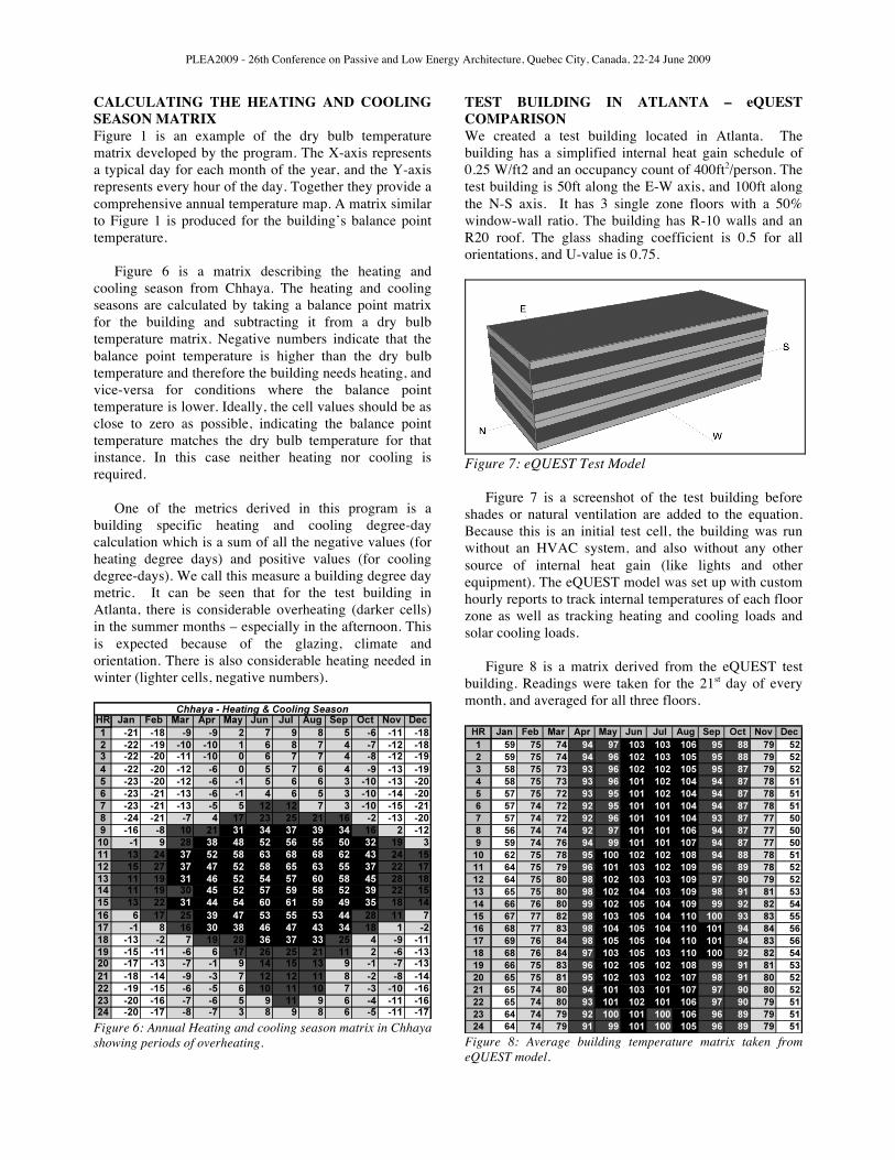
TEST BUILDING IN ATLANTA – eQUEST COMPARISON We created a test building located in Atlanta. The building has a simplified internal heat gain schedule of 0.25 W/ft2 and an occupancy count of 400ft2/person. The test building is 50ft along the E-W axis, and 100ft along the N-S axis. It has 3 single zone floors with a 50% window-wall ratio. The building has R-10 walls and an R20 roof. The glass shading coefficient is 0.5 for all orientations, and U-value is 0.75.

Figure 7: eQUEST Test Model

Figure 7 is a screenshot of the test building before shades or natural ventilation are added to the equation. Because this is an initial test cell, the building was run without an HVAC system, and also without any other source of internal heat gain (like lights and other equipment). The eQUEST model was set up with custom hourly reports to track internal temperatures of each floor zone as well as tracking heating and cooling loads and solar cooling loads.

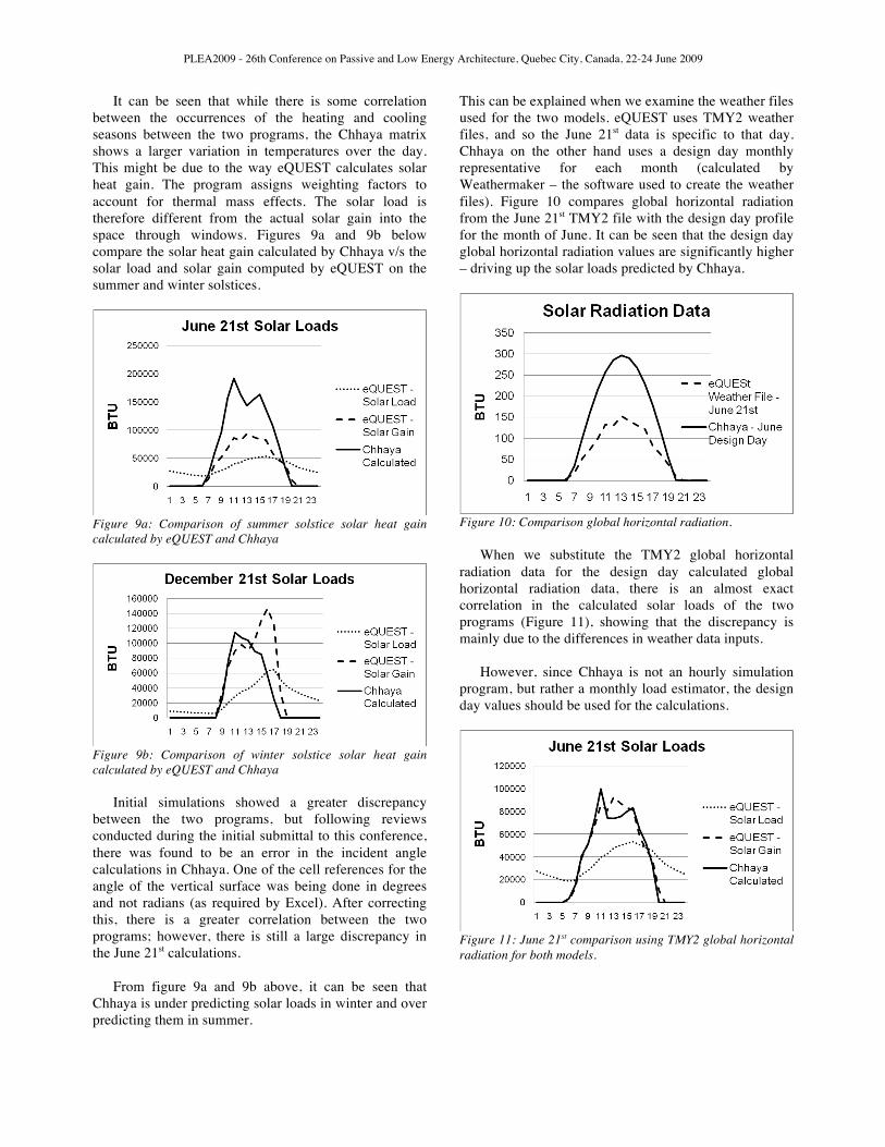
Figure 8 is a matrix derived from the eQUEST test building. Readings were taken for the 21st day of every month, and averaged for all three floors.

Figure 8: Average building temperature matrix taken from eQUEST model.


It can be seen that while there is some correlation between the occurrences of the heating and cooling seasons between the two programs, the Chhaya matrix shows a larger variation in temperatures over the day. This might be due to the way eQUEST calculates solar heat gain. The program assigns weighting factors to account for thermal mass effects. The solar load is therefore different from the actual solar gain into the space through windows. Figures 9a and 9b below compare the solar heat gain calculated by Chhaya v/s the solar load and solar gain computed by eQUEST on the summer and winter solstices.

Figure 9a: Comparison of summer solstice solar heat gain calculated by eQUEST and Chhaya

Figure 9b: Comparison of winter solstice solar heat gain calculated by eQUEST and Chhaya

Initial simulations showed a greater discrepancy between the two programs, but following reviews conducted during the initial submittal to this conference, there was found to be an error in the incident angle calculations in Chhaya. One of the cell references for the angle of the vertical surface was being done in degrees and not radians (as required by Excel). After correcting this, there is a greater correlation between the two programs; however, there is still a large discrepancy in the June 21st calculations.

From figure 9a and 9b above, it can be seen that Chhaya is under predicting solar loads in winter and over predicting them in summer.

This can be explained when we examine the weather files used for the two models. eQUEST uses TMY2 weather files, and so the June 21st data is specific to that day. Chhaya on the other hand uses a design day monthly representative for each month (calculated by Weathermaker – the software used to create the weather files). Figure 10 compares global horizontal radiation from the June 21st TMY2 file with the design day profile for the month of June. It can be seen that the design day global horizontal radiation values are significantly higher – driving up the solar loads predicted by Chhaya.

Figure 10: Comparison global horizontal radiation.

When we substitute the TMY2 global horizontal radiation data for the design day calculated global horizontal radiation data, there is an almost exact correlation in the calculated solar loads of the two programs (Figure 11), showing that the discrepancy is mainly due to the differences in weather data inputs.

However, since Chhaya is not an hourly simulation program, but rather a monthly load estimator, the design day values should be used for the calculations.

Figure 11: June 21st comparison using TMY2 global horizontal radiation for both models.


CALCULATION OF SOLAR TRANSMITTANCE The calculation of transmitted solar radiation is a product of four factors: • Incident solar radiation • Incident angle of the solar radiation on the glass • Shading coefficient of the glass • Horizontal projection of the window shade.

Figure 12: Relationship between incident angle and transmittance for clear plate glass (adapted from ASHRAE Handbook of Fundamentals).

Figure 12 is adapted from Figure 18 in Chapter 31 from the ASHRAE Handbook of fundamentals. It can be seen that the solar radiation drops off considerably when the incident angle crosses 60 degrees. The transmittance is simplified by breaking up the calculations into two formulae – for angles below 60 and angles above 60.

For incident angles below 60 degrees, the transmittance is calculated as: Ti = -9E-06I2 - 0.0004I + 0.7918 (5)

For incident angles above 60 degrees, the transmittance is calculated as: Ti = -0.0006I2 + 0.0699I - 1.2225 (6) Where Ti = transmittance through glass I = incident angle.

Thus, the solar radiation transmitted through a window is calculated as: R = IR x SCG x SCS x Ti (7) Where IR = Incident solar radiation SCG = Shading coefficient of glass

SCS = Shading provided by horizontal shade (EQ 4) Ti = Transmittance (based on incident angle) CONCLUSIONS/ FUTURE WORK This project is in a work that has been in continuous development since 2004. The new shading options as well as the ability to analyze ventilation options is one that we feel will allow architects to better explore these ideas, and ask more pertinent design questions. The ease with which the slider bars allow designers to play around with shades and window sizes, and get instantaneous feedback is invaluable to the schematic design process, allowing this to integrate early in the design process.

Future work will include a more thorough comparison with eQUEST and possibly other simulation programs. Future work will also include a variable setpoint range allowing a full utilization of the adaptive comfort range. At this point, the air change rates are guessed at by the user. We plan to derive those from window sizes and climate data. There is also work currently going on to add a thermal mass option as well as a daylighting switch (to reduce internal heat gains when light levels are high enough). REFERENCES 1. V. Sami, V. Olgyay (2004), “Calculating an Optimal Sun Angle for Window Shading”, Solar 2004 conference proceedings. 2. G. Mehta.(2007) “Appropriateness Of Natural Ventilation For Thermal Comfort In Different Climatic Regions”, Solar 2007 conference proceedings 3. 2005 ASHRAE Handbook – Fundamentals 4. ASHRAE Standard 55 – 2004. 5. ASHRAE Handbook Fundamentals - 2005 6. R.J. de Dear, G.S. Brager, “Developing an adaptive model of thermal comfort and preference”, 1998.

Documents

abstract ID 577 - Université Laval Heating and... · naturally conditioned spaces (Adapted from ASHRAE Std ... 55-2004). COOLING CAPACITY OF AIR The cooling capacity of air is obtained