COMMON SUB-EXPRESSIONELIMINATION USING SUBTREE

ISOMORPHISMS

Robert King

UUCS-19-010

School of ComputingUniversity of Utah

Salt Lake City, UT 84112 USA

December 19, 2019

Abstract

The purpose of this work is to improve the run time of the numerical simulation of bi-nary black hole mergers and the estimation of their signatures of the resulting gravitationalwave emission. Binary black hole mergers are modeled using the BSSN formulation ofthe Einstein equation. The BSSN equations consist of several complex partial differentialequations and to model these equations the value of each variable is computed once per timestep in the model. The overall model is constructed by calculating millions of timestepsto see how black holes interact with each other. Each timestep must solve the partial dif-ferential equations. This process is automated using the python package SymPy. SymPytakes mathematical expressions and generates python code to solve each expression. How-ever due to the complexity of the BSSN differential equations, the auto generated codeconsists of thousands of temporary variables. Due to the number of temporary variables,modern compilers are unable to effectively optimize the code causing the code to becomeincredibly inefficient. This thesis illustrates a technique to use Subtree Isomorphisms andcommon sub-expression elimination to improve the run time. The focus of this work isto use a bottom up approach to find an efficient way to solve for the values of the partialdifferential equations for each timestep. The strategy is to convert the all temporary vari-able computations into expression trees. Once the expression trees are created, a subtreeisomorphism analysis is performed to determine which temporary variables consist of thesame expressions. Once the subtree isomorphisms are determined, the expression trees canbe rebuilt to take advantage of caching for the targeted memory architecture.

COMMON SUB-EXPRESSION ELIMINATION USING

SUBTREE ISOMORPHISMS

by

Robert King

A thesis submitted to the faculty ofThe University of Utah

in partial fulfillment of the requirements for the degree of

Bachelors of Science in Computer Science

School of Computing

The University of Utah

Dec 2019

Approved:

/ /Hari Sundar H. James de St. GermainProfessor Director of Undergraduate StudiesSupervisor School of Computing

/Ross WhitakerDirectorSchool of Computing

Copyright c© Robert King 2019

All Rights Reserved

ABSTRACT

The purpose of this work is to improve the run time of the numerical simulation of

binary black hole mergers and the estimation of their signatures of the resulting gravi-

tational wave emission. Binary black hole mergers are modeled using the BSSN formu-

lation of the Einstein equation. The BSSN equations consist of several complex partial

differential equations and to model these equations the value of each variable is computed

once per time step in the model. The overall model is constructed by calculating millions

of timesteps to see how black holes interact with each other. Each timestep must solve

the partial differential equations. This process is automated using the python package

SymPy. SymPy takes mathematical expressions and generates python code to solve each

expression. However due to the complexity of the BSSN differential equations, the auto

generated code consists of thousands of temporary variables. Due to the number of tempo-

rary variables, modern compilers are unable to effectively optimize the code causing the

code to become incredibly inefficient. This thesis illustrates a technique to use Subtree

Isomorphisms and common sub-expression elimination to improve the run time. The

focus of this work is to use a bottom up approach to find an efficient way to solve for

the values of the partial differential equations for each timestep. The strategy is to convert

the all temporary variable computations into expression trees. Once the expression trees

are created, a subtree isomorphism analysis is performed to determine which temporary

variables consist of the same expressions. Once the subtree isomorphisms are determined,

the expression trees can be rebuilt to take advantage of caching for the targeted memory

architecture.

CONTENTS

ABSTRACT . . . . . . . . . . . . . . . . . . . . . . . . . . . . . . . . . . . . . . . . . . . . . . . . . . . . . . . . . . . . . ii

LIST OF FIGURES . . . . . . . . . . . . . . . . . . . . . . . . . . . . . . . . . . . . . . . . . . . . . . . . . . . . . . . iv

ACKNOWLEDGEMENTS . . . . . . . . . . . . . . . . . . . . . . . . . . . . . . . . . . . . . . . . . . . . . . . . v

CHAPTERS

1. INTRODUCTION . . . . . . . . . . . . . . . . . . . . . . . . . . . . . . . . . . . . . . . . . . . . . . . . . . . . 1

2. BACKGROUND . . . . . . . . . . . . . . . . . . . . . . . . . . . . . . . . . . . . . . . . . . . . . . . . . . . . . 4

2.1 BSSN Formalism . . . . . . . . . . . . . . . . . . . . . . . . . . . . . . . . . . . . . . . . . . . . . . . . . . 42.1.1 Modern Implementations . . . . . . . . . . . . . . . . . . . . . . . . . . . . . . . . . . . . . . 4

2.2 Expression Trees . . . . . . . . . . . . . . . . . . . . . . . . . . . . . . . . . . . . . . . . . . . . . . . . . . 82.3 Subtree Isomorphisms . . . . . . . . . . . . . . . . . . . . . . . . . . . . . . . . . . . . . . . . . . . . . 92.4 Centrality . . . . . . . . . . . . . . . . . . . . . . . . . . . . . . . . . . . . . . . . . . . . . . . . . . . . . . . 10

2.4.1 Degree Centrality . . . . . . . . . . . . . . . . . . . . . . . . . . . . . . . . . . . . . . . . . . . . . 102.4.2 Closeness Centrality . . . . . . . . . . . . . . . . . . . . . . . . . . . . . . . . . . . . . . . . . . 11

2.4.2.1 Betweeness Centrality . . . . . . . . . . . . . . . . . . . . . . . . . . . . . . . . . . . . . 122.4.2.2 Eigenvector Centrality . . . . . . . . . . . . . . . . . . . . . . . . . . . . . . . . . . . . 14

2.5 Auto Code Generation . . . . . . . . . . . . . . . . . . . . . . . . . . . . . . . . . . . . . . . . . . . . . 162.5.1 SymPy . . . . . . . . . . . . . . . . . . . . . . . . . . . . . . . . . . . . . . . . . . . . . . . . . . . . . . 162.5.2 Fenics . . . . . . . . . . . . . . . . . . . . . . . . . . . . . . . . . . . . . . . . . . . . . . . . . . . . . . 172.5.3 Kranc . . . . . . . . . . . . . . . . . . . . . . . . . . . . . . . . . . . . . . . . . . . . . . . . . . . . . . . 17

3. METHODOLOGY . . . . . . . . . . . . . . . . . . . . . . . . . . . . . . . . . . . . . . . . . . . . . . . . . . . . 18

3.1 Parsing . . . . . . . . . . . . . . . . . . . . . . . . . . . . . . . . . . . . . . . . . . . . . . . . . . . . . . . . . . 183.2 Staging . . . . . . . . . . . . . . . . . . . . . . . . . . . . . . . . . . . . . . . . . . . . . . . . . . . . . . . . . . 193.3 Rebuilding . . . . . . . . . . . . . . . . . . . . . . . . . . . . . . . . . . . . . . . . . . . . . . . . . . . . . . . 20

3.3.1 Greedy Algorithm . . . . . . . . . . . . . . . . . . . . . . . . . . . . . . . . . . . . . . . . . . . . 203.3.2 Adjusted Greedy Algorithm . . . . . . . . . . . . . . . . . . . . . . . . . . . . . . . . . . . . 213.3.3 Centrality Algorithm . . . . . . . . . . . . . . . . . . . . . . . . . . . . . . . . . . . . . . . . . . 21

3.4 Code Generation . . . . . . . . . . . . . . . . . . . . . . . . . . . . . . . . . . . . . . . . . . . . . . . . . . 22

4. RESULTS . . . . . . . . . . . . . . . . . . . . . . . . . . . . . . . . . . . . . . . . . . . . . . . . . . . . . . . . . . . 23

4.1 Greedy Algorithm . . . . . . . . . . . . . . . . . . . . . . . . . . . . . . . . . . . . . . . . . . . . . . . . 234.2 Adjusted Greedy Algorithm . . . . . . . . . . . . . . . . . . . . . . . . . . . . . . . . . . . . . . . . 254.3 Centrality Algorithm . . . . . . . . . . . . . . . . . . . . . . . . . . . . . . . . . . . . . . . . . . . . . . 26

5. CONCLUSION . . . . . . . . . . . . . . . . . . . . . . . . . . . . . . . . . . . . . . . . . . . . . . . . . . . . . . 29

REFERENCES . . . . . . . . . . . . . . . . . . . . . . . . . . . . . . . . . . . . . . . . . . . . . . . . . . . . . . . . . . . 30

LIST OF FIGURES

2.1 BSSN equations[28]. . . . . . . . . . . . . . . . . . . . . . . . . . . . . . . . . . . . . . . . . . . . . . . . . 5

2.2 Visualizations of meshing. . . . . . . . . . . . . . . . . . . . . . . . . . . . . . . . . . . . . . . . . . . . 5

2.3 Meshing r=1, r=10, r = 100 where r represents the mass ratio. . . . . . . . . . . . . . . . 6

2.4 Results of Fernando’s tree search. [19] . . . . . . . . . . . . . . . . . . . . . . . . . . . . . . . . . . 6

2.5 Autogenerated code from SymPy [18]. . . . . . . . . . . . . . . . . . . . . . . . . . . . . . . . . . 7

2.6 Results from BSSN Simulations using Dendro [19] . . . . . . . . . . . . . . . . . . . . . . . 8

2.7 A Binary Expression Tree Representing 3*((5+9) *2). . . . . . . . . . . . . . . . . . . . . . . 9

2.8 An Example Demonstrating Tree H is a Subtree Isomorphism of G [17] . . . . . . 10

2.9 An Example Demonstrating Degree Centrality. . . . . . . . . . . . . . . . . . . . . . . . . . . 11

2.10 An Example Demonstrating Closeness Centrality. . . . . . . . . . . . . . . . . . . . . . . . . 13

2.11 An Example Demonstrating Betweeness Centrality . . . . . . . . . . . . . . . . . . . . . . . 14

2.12 An Example Demonstrating Eigenvector Centrality. . . . . . . . . . . . . . . . . . . . . . . 15

3.1 Original Expression Tree. . . . . . . . . . . . . . . . . . . . . . . . . . . . . . . . . . . . . . . . . . . . . 18

3.2 Staged Expression Tree. . . . . . . . . . . . . . . . . . . . . . . . . . . . . . . . . . . . . . . . . . . . . . 19

3.3 Rebuilt Expression Tree. . . . . . . . . . . . . . . . . . . . . . . . . . . . . . . . . . . . . . . . . . . . . . 19

4.1 Plot comparing how number of dependencies affects the cache miss rate forthe greedy algorithm. . . . . . . . . . . . . . . . . . . . . . . . . . . . . . . . . . . . . . . . . . . . . . . . 23

4.2 Plot comparing how number of dependencies affects the run time for thegreedy algorithm. . . . . . . . . . . . . . . . . . . . . . . . . . . . . . . . . . . . . . . . . . . . . . . . . . . 24

4.3 Plot comparing how number of dependencies affects the cache miss rate forthe adjusted greedy algorithm. . . . . . . . . . . . . . . . . . . . . . . . . . . . . . . . . . . . . . . . 25

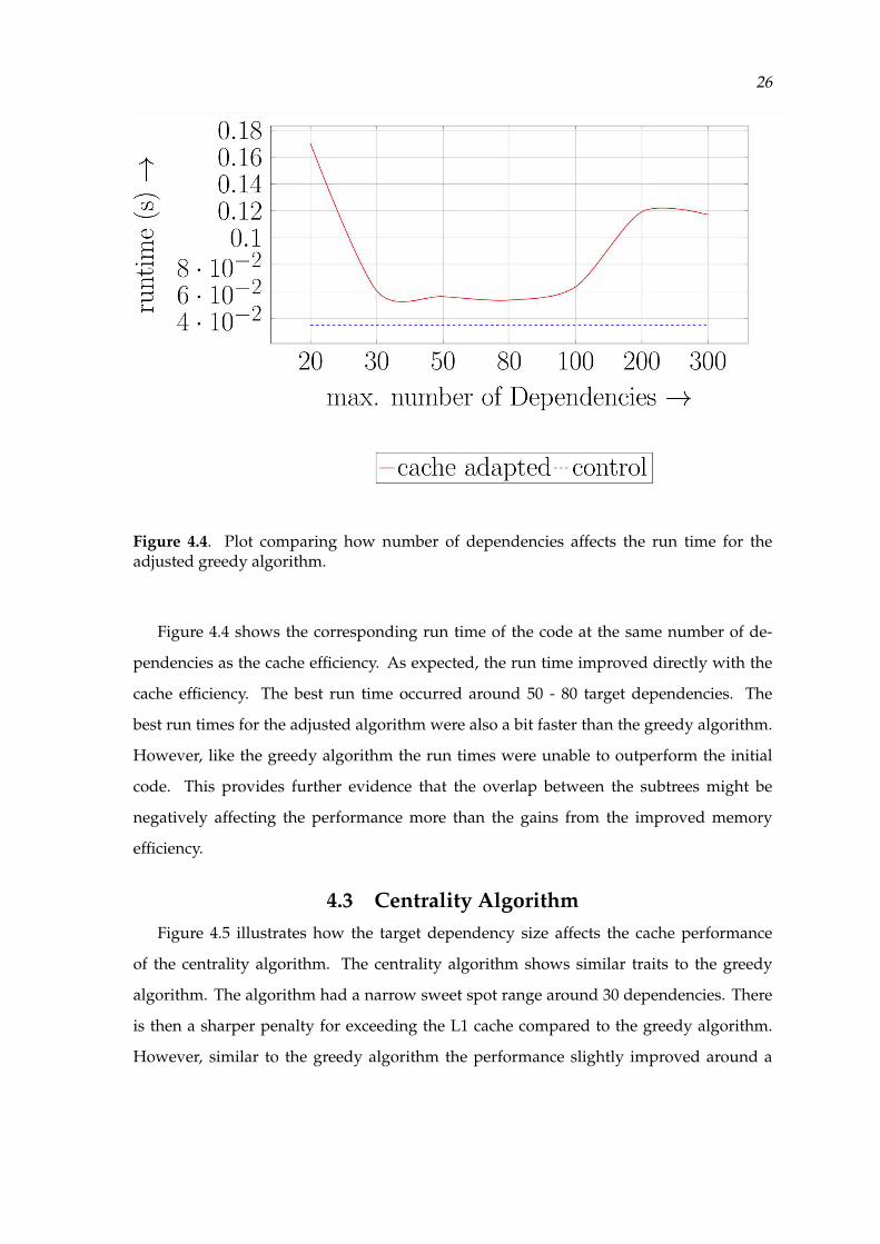
4.4 Plot comparing how number of dependencies affects the run time for theadjusted greedy algorithm. . . . . . . . . . . . . . . . . . . . . . . . . . . . . . . . . . . . . . . . . . . . 26

4.5 Plot comparing how number of dependencies affects the cache miss rate forthe centrality algorithm. . . . . . . . . . . . . . . . . . . . . . . . . . . . . . . . . . . . . . . . . . . . . . 27

4.6 Plot comparing how number of dependencies affects the run time for thecentrality algorithm. . . . . . . . . . . . . . . . . . . . . . . . . . . . . . . . . . . . . . . . . . . . . . . . . 28

ACKNOWLEDGEMENTS

This thesis would not have been possible without Professor Hari Sundar, my advisor.

CHAPTER 1

INTRODUCTION

Scientific modeling is integral to predicting the future. Modeling has been applied to

population regulation, stock market trading, race car perform ace, airplane engineering,

and space flight to name a few industries. Each of these industries use modeling to help

make informed decisions to benefit the future. Modeling allows for cheap forecast and

an improved risk analysis. Modeling significantly improved with the rise of high per-

formance computing. This thesis has created a general method to improve the memory

efficiency of modeling.

In the astrophysics community, the theoretical and experimental discovery of gravita-

tional waves has inspired new research in black holes. This thesis focuses on the modeling

of binary black hole systems. A binary black system consists of two black holes orbit-

ing one another. Due to the extreme gravitational forces being applied it is common for

gravitational waves to be produced and propagate from the system. By modeling binary

black hole systems, research aims to better understand the development of gravitational

waves and estimate potential effects of black holes and how they interact with one another.

These new insights provide better opportunities to understand the underlying physics of

extreme gravitational environments and understand how black holes are generated in the

universe.

There are several methodologies used to simulate binary black holes. In this thesis

the BSSNOK equations are used to model the physics behind black hole interactions. As

explained in more depth later in the thesis, the BSSNOK equations set realistic conditions

for two binary black holes and attempt to model the effects of the black holes on one

another through time. Modeling the forces requires several complex partial differential

equations. Problems arise when attempting to discretize the model and maintain accuracy.

In order to maintain accuracy, millions of grid points must be modeled for each time step.

2

This requires considerable computational resources.

High performance computing utilizes several computers in conjunction to solve com-

plex tasks. Typically the strongest supercomputers contain thousands of CPUs and GPUS.

The improved hardware allows for higher fidelity models at cheaper costs. The improve-

ments of high performance modeling allow breakthroughs in industry by allowing for

rapid prototyping of new materials and designs while also confirming pioneering theoret-

ical work. Most modern supercomputers have similar architectures that consist of several

computing racks in a large room. Each rack contains several computational nodes each

working with a shared memory between other computational nodes in the rack. Since

computational nodes are relatively independent of one another, it costs a considerable

amount of time to send memory between the computational nodes. As a result, memory

management is incredibly important when discretizing work for each computational node.

To improve the memory performance a deeper understanding of modern memory systems

is required.

Modern memory hierarchies balance the cost of production of memory chips with the

performance of the memory. A rule of thumb goes “the further from the CPU the larger

the memory but the slower the run time.” The fastest memory in a computer exists in the

registers within the CPU. This is the direct memory the CPU is editing. The next source

of memory is cache. The caches contain memory recently used or about to be used by the

CPU. The caches are usually broken down to levels: L1, L2, and L3 caches. For each cache

level it is about a 10x reduction in speed. The L1 cache is 10x slower than the registers, and

the L2 cache is roughly 10x slower than the L1 cache and so on. Overall the L3 cache is

1000x slower than the memory in the registers. Once the data requirement exceeds the size

of the cache then data becomes extremely expensive to load. In order to maintain efficiency

and complete simulations in a reasonable amount of time, it is paramount to be memory

efficient.

With the understanding of the costs of memory, the discussion becomes how to reduce

the memory fooprint. For most web-based programs the memory footprint is small and

not much of a concern. However for larger simulations these problems are magnified. For

the black hole modeling examined in this thesis, there are millions of grid points modeled,

and for each grid point there are thousands of temporary variables used to represent the

3

state of the simulation. The data quickly overflows the registers, L1 and L2 cache. To

avoid extreme runtime penalties, this thesis examines clever techniques to maximize the

reuse value of data in the registers and L1 cache to reduce the number of times data must

be moved.

The focus of the thesis is to perform common sub-expression elimination to avoid

duplicating the same work for each grid point in the simulation. Once the expressions

for the partial differential equations have been reduced, several algorithms are applied to

adapt the calculation for the size of the memory. The goal is to breakdown the computa-

tions into L1 bite size chunks. Each bite size is filled with data that is useful for a single

computation. Once completed, the next L1 bite size chunk if brought in and a different

computation is performed. Ideally, each chunk is mutually exclusive from one another

other to avoid repetitively loading the same data. These bite size chunks build upon each

other to calculate the necessary information for each grid point and simulate the black

holes over time.

CHAPTER 2

BACKGROUND

2.1 BSSN Formalism

In 1915 Albert Einstein completed his work of General Relativity. The monumental

work redefined how gravity and matter were perceived. Einstein demonstrated how all

matter exerting gravity warped space time. The larger the mass of the matter the more

significant the warping of space time. This reasoning culminated to the definition of a

black hole. A black hole is an object that exerts enough gravity such that light is unable to

escape from the gravitational pull [28].

Later in 1999, Thomas Baumgarte, Stuart Shapiro, Masaru Shibata and Takashi Naka-

mura developed the BSSN formalism [8, 28, 30]. The formalism models how black holes

collide and models how the resulting gravitational waves evolve after the collision. The

BSSN equations, as seen in Figure 2.1, set realistic initial conditions by solving constraint

equations and proceed to use the constraints to solve Einsteins equations. These equa-

tions consist of several complex partial differential equations. By solving the equations

at hundreds of thousands of timesteps an accurate model can be produced. This has

been implemented in various open source projects like the Einstein toolkit, and Cactus

Computational toolkit [8, 13, 19].

2.1.1 Modern Implementations

The discovery of gravitational waves has encouraged new research on modeling gravi-

tational waves. At the University of Utah, the Dendro-Gr work done by Milinda Fernando

analyzes new strategies to model binary black holes [19]. Fernando has created a fully

wavelet adaptive mesh, seen in Figure 2.2, automatic code generation, a new parallel

search algorithm named TreeSearch to model mass ratios up to 100 for gravitational waves.

Figure 2.2 the wavelet adaptive mesh. The wavelet mesh determines the number of

5

Figure 2.1. BSSN equations[28].

Figure 2.2. Visualizations of meshing.

points within a specified mesh area. Once the number of points surpasses a specified

epsilon upper bound then the mesh refines itself into several smaller meshes until the

number of points is smaller than the specified epsilon value. As the refinement of the mesh

increases, it begs the question whether the simulation will be able to scale well. Fernando

showed the epsilon value to be inversely related to the the size of the mass ratio of the

black hole being modeled. In doing so the mesh is able to scale O(n3) with respect to the

mass ratio. Figure 2.3 illustrate the scaling mesh.

Once the mesh has been developed it is critical to be able to send information near the

6

Figure 2.3. Meshing r=1, r=10, r = 100 where r represents the mass ratio.

bounds of each block to nearby blocks. This requires a search of nearby points and if points

are within a nearby mesh. This part is critical because an inefficient implementation causes

serious memory inefficiency and poor run time.

To maintain efficient run time a new search algorithm was developed [19]. This al-

gorithm utilizes adaptive octrees to create a search algorithm with O(n) complexity for

the entire simulation compared to the O(n log n) complexity used in the common binary

search for the entire simulation. Figure 2.4 illustrates the improvement once the simulation

contains several million data points.

Figure 2.4. Results of Fernando’s tree search. [19]

In addition to providing new and exciting computational performance to simulating

black holes, Fernando’s work also introduced using auto generated code. The auto gen-

erated code is used to convert mathematical notation into high performance C code using

the package SymPy, seen in Figure 2.5. In addition to adding convenience, the code

7

allows complex differential equations to be discretized effectively and efficiently. The auto

generated code presented in this paper was critical for this thesis and was the starting

point for the common sub-expression elimination analysis.

Figure 2.5. Autogenerated code from SymPy [18].

With these new developments, Fernando was able to collect excellent results, seen in

Figure 2.6 and demonstrate excellent scaling for the binary black hole simulation [19].

Looking at the results, the rhs calculations, in green, account for approximately 20% of

the computational cost. The rhs calculations are calculating the state of each point in

the simulation. Each of these points is calculated on its own computational node. Each

of these calculations required thousands of temporary variables to solve efficiently. The

auto generated code, while effective does not adapt for the memory architecture of the

computational node. In doing so, this presents an opportunity to adapt the auto generated

code for the memory architecture of the system. This is the main focus of the thesis.

8

Figure 2.6. Results from BSSN Simulations using Dendro [19]

2.2 Expression Trees

Expression trees are a tree representation of mathematical expressions. In an expres-

sion tree, the leaf nodes represent constants or variables while non-leaf nodes represent

different operators on the tree. For this work the expression trees were binary expression

trees. In a binary expression tree, each node must have either zero children, if the node

is a leaf, or exactly 2 children to represent the left-hand side and right-hand side of each

operation. An expression tree can be created easily using two stacks. The first stack keeps

track of constants while the second stack keeps track of the operators.

The expression tree, seen in Figure 2.7 can be constructed by popping off the first values

of the the constants stack and becoming the leaf nodes to the top operator in the operator

stack. The new tree consisting of a single operator and two constants can be placed

onto the constants stack. This process can be repeated until a single constant remains

on the constant stack or no operators remain on the operator stack. Slight variations of

this algorithm are necessary depending on the types of operators used in the expression

tree to maintain order of operations. For complex non-binary expression trees, a dynamic

programming approach can be used to solve the tree using the algorithm discussed by

9

Figure 2.7. A Binary Expression Tree Representing 3*((5+9) *2).

Aho and Johnson [2]. Additionally, these trees can be manipulated to solve the max flow

problem or multiple expression trees can be joined using O(n) space and O(log(n)) query

time as presented in Chohen and Tamassias work [6].

2.3 Subtree Isomorphisms

A subtree isomorphism is defined as one tree being identical in shape to another tree.

When determining if a subtree isomorphism exists, it is critical to consider reflection of

each subtree. Abboud [1] gives an overview of the subtree isomorphism problem and

concludes his work by demonstrating it is extremely unlikely to solve the subtree isomor-

phism problem in subquadratic complexity.

Subtree Isomorphism problems were introduced by Matula [17] in 1968. Reyner [24]

expanded Matulas work and demonstrated that the subtree isomorphism problem can be

bounded by O(n2.5) for trees of any degree. The algorithm is developed by calling several

recursive calls to check all possible subtrees. However, for binary subtree isomorphism the

complexity can be reduced to O(n2). Matulas work was improved by Shamir and Tsur by

demonstrating a O( k1.5

logk )n) algorithm for subtree isomorphisms [27].

10

Figure 2.8. An Example Demonstrating Tree H is a Subtree Isomorphism of G [17]

2.4 Centrality

Centrality is a common problem studied in graphs. The goal of centrality is to find

critical or central nodes of the graph. The definition of critical nodes can change depending

on the problem but centrality is critical for network, pipe flow, social network, game theory

and traffic problems [4, 7]. In addition to finding critical nodes, it is important to find

critical nodes efficiently. In this thesis, centrality will be used to help identify critical nodes

in expression trees.

When comparing the centrality of nodes it is common to normalize the centrality value

of the nodes in the graph. The centrality measure is commonly denoted as ci for each node.

The best centrality score, c∗ is defined as:

c∗ = max{c1, ..., cn}

The importance of the central node is commonly defined as:

S = ∑i

[c∗ − ci]

Using this notation a significant node exists in the graph if S is large. If S = 0 then all

the nodes in the graph have the same weight.

2.4.1 Degree Centrality

Degree Centrality stems from the idea that important nodes have many connections in

the graph. Depending on the graph there are three main degree centrality measurements:

11

undirected degree centrality, outdegree centrality, indegree centrality.

undirected = cdi = ∑

j:j 6=i

yi,j

outdegree = coi = ∑

j:j 6=i

yi,j

indegree = cii = ∑

j:j 6=i

yj,i

Figure 2.9. An Example Demonstrating Degree Centrality.

In Prell’s paper [23] they discuss how degree centrality scales very well and can be used

to quickly determine the key stake holders in social networks for resource management.

One caveat of using the degree centrality is that it does not give a strong measure of the

connectiveness of the surrounding graph around the central nodes. The paper argues that

it is better to use metrics like closeness and betweeness centrality for these scenarios [23].

2.4.2 Closeness Centrality

Closeness centrality stems from the idea that a central node is on average close to other

nodes. Specifically a distance and centrality metric are necessary to determine central

nodes. The distance, di,j is commonly defined as the number of edges connecting one

12

node to another. Centrality is measured by 1 over the average distance of a node to all

other nodes in the graph, and is defined as follows:

cci =

1

∑j:j 6=i di,j=

1

(n − 1)d̄i

As the average distance between nodes decreases the overall centrality score increases.

Closeness centrality is also commonly standardized among the nodes in a graph. The

maximum score occurs when a single node is within a single edge distance to all other

nodes in the graph.

cdmax =

1

n − 1

The standardization can be defined as follows:

c̃ci =

cci

ddmax

= (n − 1)cci =

1

d̄i

Closeness centrality performs best in characterizing a node’s importance when direct

connections are not as important but overall connectiveness is ideal. However, Closeness

Centrality does not perform as well when there are significant outliers or breaks within the

graph. Rochat [25] proposes a solution to compensate for breaks in the graph by using a

technique call harmonic centrality. This approach slightly adjusts the the original formula

of the inverse of the sum of distances to the sum of inverted distances:

original : cci =

1

∑j:j 6=i di,j

harmonic : cci = ∑

i 6=j

1

di,j

Closeness centrality is extremely commonly used in social network analysis. Top-k

approache metrics are often used to determine which people to target for maximum ad

impact [20]. Additionally, these metrics have been used to measure websites on the inter-

net and food webs in the animal kingdom [7].

2.4.2.1 Betweeness Centrality

Betweeness centrality originates from the idea that a central node acts as a limiting

pathway from one part of the graph to the other. Strong betweeness nodes create a path

13

Figure 2.10. An Example Demonstrating Closeness Centrality.

between unlinked nodes, also known as a geodesic. The central nodes lie on several

geodesics between other nodes in the graph. Some important notation to define betwee-

ness centrality:

gj,k = number of geodesics between nodes j and k.

gj,k(i) = number of geodesics between j and k that pass through i.

cbi = ∑

j<k

gj,k(i)

gj,k

The formula for centrality can be interpreted as the probability that a given path from

j to k passes through i. For disconnected parts of the graph it is common to treat the

probability as zero in the sum. The centrality is standardized using the following formula:

14

c̃bi =

2cbi

(n − 1)(n − 2)

Figure 2.11. An Example Demonstrating Betweeness Centrality

Betweeness centrality is especially used to identify bottlenecks in graphs or networks.

Borgatti also demonstrates that the likelihood flow may not take the shortest path from

one node to another depending on the incoming flow to a central node is extremely high

[4]. One negative to betweeness centrality is the complexity to determine the centrality

value of each node. Several works have been done to reduce the complexity from O(V3) to

O(V2logV + VE)) [5, 10].

2.4.2.2 Eigenvector Centrality

Eigenvector centrality is the best known centrality metric [4]. It became infamous

as an instrumental tool in the original PageRank algorithm used by Google [21]. The

algorithm determines central nodes by taking the rankings of neighbors into consideration

when determining a node’s own ranking. The process is calculated by determining the

eigenvectors of the matrix mapping each node to one another. The corresponding ranking

of each node is reflected in the eigenvector. This can be represented mathematically as

follows:

15

cei =

1

λ∑

j:j 6=i

yi,jcej

This is represented in matrix algebra using the following:

Yce = λce

where Y represents the matrix edge mapping between nodes. Figure 2.12 illustrates

how eigenvector centrality rates nodes in practice. Notice how the nodes with a large

number of connection are weighted higher near the edge of the graphs and how the rating

cascades into the middle of the graph.

Figure 2.12. An Example Demonstrating Eigenvector Centrality.

Eigenvector centrality has a minor problem when trying to rank fake nodes in the

graph. This was common problem for Google since websites attempt to gain better view-

ership. Haveliwala illustrates techniques to adjust scores based on categorizing zombie

pages that have no viewership [9]. Additionally, eigenvector centrality has been extended

to multiplex networks to help be able to identify important nodes in machine learning

networks [29]. Eigenvector centrality also has had a tremendous impact on brain research.

When subjects are stimulated performing a variety of task from motor action, art, and

mathematics, different areas of the brain become active and the critical areas for each task

can be mapped using centrality techniques [16].

16

2.5 Auto Code Generation

Auto code generation is a new approach to break down complex tensors, partial dif-

ferential equations or large expression trees into manageable sizes for compilers. Modern

day compilers balance the costs of fast code and reasonable compile times. These two ob-

jectives are often counteracting forces. For complex problems, the common sub-expression

elimination (CSE) can be complex and time consuming. Instead of completing the CSE, the

compiler weights the computational cost of the reduction, and if the compiler judges the

operation as time inefficient, the compiler will not reduce the code. This is understandable

since users do not want to wait significant amounts of time to compile code.

Auto generation code provides an alternative to compilers by ignoring the computa-

tional cost of the common sub-expression elimination. These techniques become more

prevalent in larger simulation codes [11, 15, 18]. By utilizing an auto code generator, the

compile times are significantly longer, often to the order of 10 to 100x slower but the

runtime improves dramatically. With large simulation, the overall gain in run time and

decreased cost justifies the longer compile time. Currently, there are three significant codes

in the simulation industry: SymPy, Fenics, and Kranc.

2.5.1 SymPy

SymPy is a library for symbolic mathematics with the goal to be a computer algebra

system. SymPy is built upon the python library and extends useful tools for tensor alge-

bra, chemistry, numerical general relativity, geometric algebra, Monte Carlo methods and

statistical modeling [12, 18, 26]. Furthermore, SymPy is built upon Python and has a low

barrier of entry. This allows for quick adaptation to large prexisting codes. This thesis

focuses on the common sub-expression elimination and code generation features.

SymPy’s common sub-expression elimination is able to perform all compiler improve-

ments and long term forecasting common sub-expression elimination. This allows for high

level mathematical operations be able to scale effectively for partial differential equation

solvers and complex statistics [26]. This reduces the technical hurdle for many scientists.

In addition to providing long term common sub-expression elimination, SymPy provides

code generation targeting high performance C code [12]. Once generated the code can be

sent to the C compiler and the simpler expressions can be optimized by the compiler.

17

The SymPy common sub-expression (CSE) modules do not take caching into account

and as a result there tends to be poor memory performance. However, the overall gain

from the optimization overshadow the memory issues. This thesis aims to improve the

cache efficiency of the common sub-expression elimination.

2.5.2 Fenics

Fenics is a code generator specific for partial differential equations [15]. Similar to

SymPy, Fenics is built upon python and target generating fast C code. Additionally, the

Fenics library can target muli-processor parallel computing using mpi in the code gener-

ation [14]. The produced code is able to create high fidelity models ranging from com-

putational fluid dynamics to biological protien folding [3]. The code has been praised by

allowing scientists to quickly take mathematical formulations and deploy simulations to

high performance codes.

2.5.3 Kranc

Kranc is another partial differential equation code generator that targets mathematica

[11]. Kranc is also used as part of the Cactus Computation toolkit [8]. Kranc is also able

to develop parallel code using OpenMp for multi-core workstations as well as providing

a common sub-expression elimination module for high performance applications. Kranc

was specifically developed form tensor equations [11]. The code was able to reduce the

runtime of previous Cactus Eintsein simulations by 38% on Intel Pentium Processors.

CHAPTER 3

METHODOLOGY

The research for this thesis consists of four distinct phases: initial parsing, staging,

rebuilding, and code generation. The goal is to create an algorithm that will be able to

analyze the different partial differential equations and reorder the temporary variable

calculations to maximize cache effectiveness and variable reuse. To implement the sub-

tree isomorphism the problem is broken up into a staging phase, focusing on finding the

isomorphisms and a rebuilding phase, that creates the optimal expression tree.

Figure 3.1. Original Expression Tree.

3.1 Parsing

The focus of the Parsing phase is to translate the the BSSN equations from mathematical

notation into Python code. This process is done using the SymPy package. SymPy is

a project that is focused on creating high performance code for mathematical notation.

Additionally, SymPy contains simple common sub-expression elimination (CSE) support.

SymPy’s CSE is able to identify simple CSE within a single mathematical expression. Once

complete, SymPy auto generates the python code. From here the SymPy auto generated

19

Figure 3.2. Staged Expression Tree.

Figure 3.3. Rebuilt Expression Tree.

code needs to be parsed into an expression tree. The sources of the tree represent the target

variables that are necessary to compute the BSSN equations at each time step.

3.2 Staging

Staging is focused on finding variable reuse within the partial differential equations.

The first problem is to create an expression tree from the partial differential equations

generated from the SymPy auto generated code. This can be done utilizing two stacks.

One that keeps track of operators and another that keeps track of values.

Once the expression tree is created, subtree isomorphism analysis can begin. This

will be a bottom up approach that starts with the leaf nodes of the tree and works up

20

using ideas from Pelegr-Llopart and Graham [22]. The subtree isomorphism will need to

consider the values used in each leaf node in addition to finding similar tree structure. This

can be done using sets. Each node within the tree will keep track of all the leaf values that

it depends on. Set similarity will be used as a precondition before calculating the more

expensive tree isomorphism. The tree isomorphism algorithm will follow loosely from the

work explained in the Background subsection. By the end of the staging process the most

common sub-expressions will be identified. Each expression will be valued depending on

the number of leaf node dependents, to mitigate the total number of temporary variables,

and the number of times each expression appears, to maximize data reuse.

3.3 Rebuilding

The rebuilding phase takes the results from the staging process and determines the

order in which the expression tree is evaluated. In order of importance, the rebuilding

phase must preserve the correct final answers, maximize cache effectiveness, and minimize

the total number of temporary variables used. The tricky part is the decision making

process to determine the best subtrees to evaluate first.

This thesis outlines three approaches to subtree decision making process: Greedy Al-

gorithm, Adjusted Greedy Algorithm, Centrality Algorithm.

3.3.1 Greedy Algorithm

The greedy algorithm uses the user specified cache size of the machine. The algorithm

scans subgraphs and looks for subtrees whose dependencies are as close as possible to the

specified cache size without exceeding the cache size. This is a quick and efficient process.

This process is outlined by starting at the sources in the DAG and using a breadth-first

search until the nodes visited have fewer dependencies than the user specified cache size.

Upon doing so, the nodes in the queue will be scanned to determine the ideal subtree.

Once an ideal subtree is identified, it is removed from the graph and the remaining

nodes’ dependencies are updated. This process is repeated until all sources in the graph

contain fewer dependencies than the user specified cache size.

21

3.3.2 Adjusted Greedy Algorithm

The greedy algorithm can perform poorly when there is significant overlap within the

expression graph. It is possible for a subgraph to be a dependency of multiple targets

and as a result the subgraph could be computed twice. This duplication can be seen in

Figure 3.3, which uses a cache size of 3. The subgraph that begins with id17 is duplicated

in two trees. When using the the original greedy algorithm the subgraph is duplicated

twice. To avoid this inefficiency, an adjusted greedy algorithm is considered.

The updated algorithm changes the greedy criterion from the number of dependen-

cies in a subgraph to the number of dependencies that the subgraph removes from the

entire graph with the restriction that the number of dependencies is smaller than the user

specified cache size.

This algorithm is outlined as follows. Initially nodes with fewer dependencies than the

user specified cache size are considered. Using a breadth-first search, nodes are visited

starting with the target source of the subtree. As each node is visited an in-degree counter

is marked. If the in-degree counter is the same as the in-degree of the node then the node

is added to the queue. Once reaching the sinks in the subgraph, if the in-degree counter is

the same of the in-degree of the sink then the sink is considered to be potentially removed

from the graph. If the counter and the in-degree of the node are not the same then the

node is required in another subgraph and cannot be removed. Once the breadth-first

seach is completed, each target subgraph is assigned a score based on the sum of the

dependencies potentially removed from the graph. The best subgraph maximizes the the

number of dependencies removed from the graph. Once an ideal subtree is identified,

it is removed from the graph and the remaining nodes’ dependencies are updated. This

process is repeated until all sources in the graph contain fewer dependencies than the user

specified cache size.

3.3.3 Centrality Algorithm

The Centrality Algorithm will be able to to target subtrees by using Betweeness Central-

ity. The goal is to identify subtrees that are necessary to multiple nodes and to extract the

subtree into a single temporary variable. By doing so the entire subtree can be represented

concisely and maximize spatial reuse since the subtree has a large centrality value. A

22

potential concern is the target subtree’s dependencies will exceed the user provided cache

size. To avoid this problem subtrees will start at nodes as close to the cache size without

exceeding the cache size.

Once the target subtree is identified, it will be removed from the computational graph

and the corresponding dependencies updated. This algorithm will repeat itself until the

sources of the computational tree’s dependencies do not exceed the user provided cache

size.

3.4 Code Generation

Once an expression tree has been reduced into subgraphs, the corresponding code

for each subgraph needs to regenerated. The process is quick compared to the other

parts. This can be done using recursion and memoization. For each node if the node is

a source then a corresponding temporary variable is created; if the node is a sink then the

node’s value is produced and finally if the node is not a source nor a sink then code is

generated based on the left child’s code, the current node’s operator and the right child’s

code generation. This process is can be expedited by caching the code for each node.

CHAPTER 4

RESULTS

The following results were collected using the University of Utah’s Center for High

Performance Computing Kingspeak supercomputer computing cluster. The Kingspeak

cluster consists of Intel Sandybridge processors with 64 KB per core L1 cache, 256 KB per

core L2 cache and 20 MB shared L3 cache size.

4.1 Greedy Algorithm

Figure 4.1. Plot comparing how number of dependencies affects the cache miss rate for thegreedy algorithm.

Figure 4.1 illustrates how the target dependency size for the subtrees affects the over-

all cache performance of the program. The graph indicates there is a clear sweet spot

24

in efficiency around 30 dependencies. With 30 dependencies as the target, the overall

cache misses decreased over 5%. Compared to the original code, which contained a cache

miss rate of 9%, the Greedy algorithm was able to increase the effectiveness of the L1

cache. Interestingly once the cache size target increased to 50 there was a slight increase in

cache performance. This suggests that the L1 cache was filling up and the subtrees were

slightly overflowing into the L2 cache. Furthermore, as the target increased to 80 and 100

dependencies the efficiency continued to improve. This suggests that the size of the target

subtrees are able to fit nicely within the L2 cache. However, the performance was not quite

as good as the target size of 30. This can be explained as more data needs to be loaded

from the L2 cache into the L1 cache.

Figure 4.2 shows at the corresponding run time of the code at the same number of

dependencies as the cache efficiency. As expected, the run time improved directly with

the cache efficiency. The best run time occurred around 30 target dependencies. However,

none of the generated codes was faster than the initial code. This suggests either the mem-

ory allocated for the subtrees is inefficient or some subtrees have considerable overlap.

Figure 4.2. Plot comparing how number of dependencies affects the run time for thegreedy algorithm.

25

4.2 Adjusted Greedy Algorithm

Figure 4.3. Plot comparing how number of dependencies affects the cache miss rate for theadjusted greedy algorithm.

Figure 4.3 illustrates how the target dependency size for the subtrees affects the over-

all cache performance of the program. Compared to the greedy algorithm the Adjusted

Greedy Algorithm has a much larger sweet spot. The Adjusted algorithm had relatively

similarly performance for cache target sizes between 50 and 80 dependencies. Addition-

ally, it is important to note that the sweet spot has slight shifted towards larger depen-

dencies. This can be attributed to the adjusted Greedy Algorithm considering how many

dependencies are removed from the graph. By considering the dependencies that are

removed from the expression tree, the corresponding dependencies only need to be loaded

into the cache once. This is maximizing the spatial reuse of each expression tree. The shift

to larger dependencies is most likely due to the target dependencies consistently being an

overestimate of the total number of dependencies being removed from the expression tree.

Roughly speaking, the number of dependencies removed from the graph from any given

subtree was approximately 80% of the target.

26

Figure 4.4. Plot comparing how number of dependencies affects the run time for theadjusted greedy algorithm.

Figure 4.4 shows the corresponding run time of the code at the same number of de-

pendencies as the cache efficiency. As expected, the run time improved directly with the

cache efficiency. The best run time occurred around 50 - 80 target dependencies. The

best run times for the adjusted algorithm were also a bit faster than the greedy algorithm.

However, like the greedy algorithm the run times were unable to outperform the initial

code. This provides further evidence that the overlap between the subtrees might be

negatively affecting the performance more than the gains from the improved memory

efficiency.

4.3 Centrality Algorithm

Figure 4.5 illustrates how the target dependency size affects the cache performance

of the centrality algorithm. The centrality algorithm shows similar traits to the greedy

algorithm. The algorithm had a narrow sweet spot range around 30 dependencies. There

is then a sharper penalty for exceeding the L1 cache compared to the greedy algorithm.

However, similar to the greedy algorithm the performance slightly improved around a

27

Figure 4.5. Plot comparing how number of dependencies affects the cache miss rate for thecentrality algorithm.

target of 100 dependencies. However, the centrality algorithm is more sensitive with

respect to the cache sizes. It appears critical to get the correct size for target cache size

for the centrality algorithm.

Figure 4.6 shows the overall run time of the simulation using the centrality algorithm.

Initially the run time appears far more erratic compared to the previous algorithms. How-

ever, the run time does improve with respect to the best cache efficiencies. Interestingly, the

run time with the best cache performance, target size of 30, is slower than the run time with

the second best cache performance, 100 dependencies. Both plots stress the heavy reliance

on using the exact target size for the machine for the best performance. However, similar

to the previous algorithms none of the run times for the centrality algorithm were able

to outperform the control code. These finding suggest that while the memory efficiency

is improving considerably, the expected run time benefits are being overshadowed by a

penalty somewhere else in the code.

28

Figure 4.6. Plot comparing how number of dependencies affects the run time for thecentrality algorithm.

CHAPTER 5

CONCLUSION

This thesis presents work to develop a generic algorithm to adapt large complex ex-

pressions for machine memory architecture with the goals of maintaining correct final

answers, maximizing cache effectiveness, and minimizing the total number of temporary

variables used. Modern high fidelity supercomputers are able to model complex phenom-

ena predominately using complex partial differential equations. To combat the increased

power and time demands to simulate models, this thesis presents techniques to adapt the

simulation’s implementation for the specific hardware architecture that the simulation is

being performed on. Due to the complexity of the problems being modeled, it is common

for the necessary memory to overflow the L1 and L2 caches. This theis presents several

strategies to increase the memory efficiency of these algorithms.

In this thesis the algorithms described were tested on the BSSN equations that model

binary black hole mergers. The experiments were run on the Kingspeak supercomput-

ing machines at the University of Utah. The algorithm presented utilized common sub-

expression elimination using subtree isomorphisms. The subtrees were identified using

three algorithms: Greedy Algorithm, Adjusted Greedy Algorithm, Centrality Algorithm.

All the algorithms improved the cache performance of the simulation and maintained

correctness of the algorithms. The best algorithms improved the cache performance 300%.

However, the corresponding run time of the algorithms did not improve compared

to the control experiment. These problems could be a result of duplicated calculations

across subtrees or memory being allocated inefficiently. These issues offer future research

opportunities.

REFERENCES

[1] A. Abboud, A. Backurs, T. Hansen, V. Williams, and O. Zamir, Subtree Isompor-phism Revisited, Proceeding, of the twenty-seventh annual symposium on DiscreteAlgorithms, pp. 1256-1271 (2016).

[2] A. Aho and S. Johnson, Optimal Code Generation for Expression Trees, ACM, 23, Issue3,pp. 488 501 (1976).

[3] Alnaes, MArtin and Blechta, Jan and Hake, Johan and Johansson, August,

and Kehlet, Benjamin and Logg, Anders and and Rognes, Marie and Wells,

Garth, The FEniCS Project Version 1.5, Lecture Notes in Computational Science andEngineering, 84 (2012).

[4] S. Borgatti, Centrality and Network Flow, Sunbel International Social Networks Con-ference, 27, Issue 1, Pages 55-71 (2005).

[5] J. Chen, D. Friesen, and H. Zheng, Tight Bound on Jonson’s Algorithm for MaximumSatisfiability, Science Direct, 58, Issue 3, pp 622-640 (1999).

[6] R. Cohen and R. Tamassia, Dynamic Expression Trees and their Applications, ProceedingSODA 91 Proceedings of the second annual ACM-SIAM symposium, ACM, pp. 52-61(1991).

[7] E. Estrada and J. Rodriguez-Velaquez, Subgraph Centrality in Complex NEtworks,Physics Review, 71, issue 5 (2005).

[8] T. Goodale, G. Allen, G. Lanfermann, J. Masso, T. Radke, E. Seidel, and

J. Shalf, The Cactus Framework and Toolkit: Design and Applications. In Vector andParallel Processing, International Conference on High Performance Computing forComputational Science, 257, pp. 197 227 (2002).

[9] T. Haveliwala, Topic-Sensitive PageRank, Proceedings of the 11th international confer-ence on World Wide Web, 1, Pages 517-526 (2002).

[10] Hougardy, Stefan, The Floyd-Warshall Algorithm on graphs with Negative Cycles, Sci-ence Direct, 110, Issue 8-9, pp 279-281 (2010).

[11] S. Husa, I. Hinder, and C. Lechner, Kranc, A Mathematica package to Generate Numer-ical Codes for Tensorial Evolution Equations, Science Direct, 174, Issue 12, pp 983 - 1004(2006).

[12] Joyner, David and Certik, Ondrej and Meurer, Aaron, and Granger, Brian,Open Source Computer Algebra Systems: SymPy, ACM Communication in ComputerAlgebra, 45, Issue 3, pp 225-234 (2011).

31

[13] F. Loffer, J. Faber, E. Bentivegna, T. Bode, P. Diener, R. Haas, I. Hinder,

B. Mundim, C. Ott, E. Schnette, G. Allen, M. Campanelli, and P. Laguna,The Einstein Toolkit: A Community Computational Infrastructure for Relative Astrophysics,Classical and Quantam Gravity, 29,Issue 11,pp. 115001 (2012).

[14] Logg, Anders and Mardal, Kent-Andre and Wells, Garth, Automated Solutionof Differential Equations by the Finite Element Method, Springer Heidelber DordrechtLondon New York, 2012.

[15] Logg, Anders and Olgaard, Kristian and Rognes, Marie and Wells, Garth,FFC:The FEniCS form Compiler, Lecture Notes in Computational Science and Engi-neering, 84 (2012).

[16] G. Lohmann, D. Margulies, A. Horstmann, B. Pleger, J. Lepsien, and D. Gold-

hahn, Eigenvector Centrality Mapping for Analyzing Connectivity Patterns in fMRI Dataof the Human Brain, PLOS, One, (2010).

[17] D. Matula, Subtree isomorphism in O(n5/2) , Annals of Discrete Mathematics, 2, pp.91-106 (1978).

[18] A. Meurer, C. Smith, M. Paprocki, O. Certik, S. Kirpicheb, M. Rocklin, A. Ku-

mar, S. Ivanov, and J. Moore, SymPy: Symbolic Computing in Python, PeerJ ComputerScience, 3 (2017).

[19] D. Neilson, M. Fernando, H. Sundar, and E. Hirschmanna, Dendro-GR: A scal-able framework for Adaptive Computational General Relativity on Heterogeneous Clusters,American Physical Society, 64 (2019).

[20] K. Okamoto, W. Chen, and X.-Y. Li, Rankings of Closeness Centrality for Large-ScaleSocial Networks, Springer Link, 5059, pp 186-195 (2009).

[21] L. Page, S. Brin, R. Motwani, and T. Winograd, The PageRank Citation Ranking:Bringing Order to the Web., Technical Report 1999-66, Stanford InfoLab, November1999. Previous number = SIDL-WP-1999-0120.

[22] E. Pelegr-Llopart and S. Graham, Optimal Code Generation for Expression Trees: anApplication BURS Theory, Proceedings of the 15th ACM SIGPLAN-SIGAT symposiumon Principles of programming languages, (1998).

[23] C. Prell, K. Hubacek, and M. Reed, Stakeholder Analysis and Social Network Analysis,Society and Natural Resources, 22, Issue 6, pp 501-518 (2009).

[24] S. Reyner, An analysis of a good algorithm for the subtree problem , SIAM Journal onComputing, 18, Issue 5, pp. 906-908 (1989).

[25] Y. Rochat, Closeness Centrality Extended To Unconnected Graphs: The Harmonic Central-ity Index, Semantic Scholar, (2009).

[26] Rocklin, Matthew and Terrel Andy, Symbolic Statistics with SymPy, AIP Computerin Science and Engineering, 14 Issue 3 (2012).

[27] R. Shamir and D. Tsur, Faster Subtree Isomorphisms, Journal of Algorithms, AcademicPress, 33, Issue 2, pp. 267-280 (1999).

32

[28] M. Shibata, Numerical relativity, World Scientific, (2015).

[29] L. Sola, M. Romance, R. Criado, J. Flores, A. Garcia, and S. Boccaletti, Eigen-vector Centrality of Nodes in Multiplex Networks, Chaos: An Interdisciplinary Journal ofNonlinear Science, 23, Issue 3 (2013).

[30] S. Williams, A. Waterman, and P. D., Introduction to 3+1 numerical relativity, OxfordUniv. Press, 140 (2008).