Quantum Structure in Cognition

Diederik AertsCenter Leo Apostel for Interdisciplinary Studies

Department of Mathematics and Department of PsychologyVrije Universiteit Brussel, 1160 Brussels, Belgium

E-Mail: diraerts@vub.ac.be

Abstract

The broader scope of our investigations is the search for the way in which concepts and their combinationscarry and influence meaning and what this implies for human thought. More specifically, we examine theuse of the mathematical formalism of quantum mechanics as a modeling instrument and propose a generalmathematical modeling scheme for the combinations of concepts. We point out that quantum mechanicalprinciples, such as superposition and interference, are at the origin of specific effects in cognition related toconcept combinations, such as the guppy effect and the overextension and underextension of membershipweights of items. We work out a concrete quantum mechanical model for a large set of experimental dataof membership weights with overextension and underextension of items with respect to the conjunctionand disjunction of pairs of concepts, and show that no classical model is possible for these data. We putforward an explanation by linking the presence of quantum aspects that model concept combinationsto the basic process of concept formation. We investigate the implications of our quantum modelingscheme for the structure of human thought, and show the presence of a two-layer structure consisting ofa classical logical layer and a quantum conceptual layer. We consider connections between our findingsand phenomena such as the disjunction effect and the conjunction fallacy in decision theory, violationsof the sure thing principle, and the Allais and Elsberg paradoxes in economics.

Keywords: concept theories, concept conjunction, guppy effect, overextension, quantum me-chanics, interference, superposition, Hilbert space, Fock space.

Introduction

To understand the mechanism of how concepts combine to form sentences and texts and carry and commu-nicate meaning between human minds is one of the major challenges facing the study of human thought.In this article we will further elaborate the theory about the combination of concepts that was initiatedin Gabora and Aerts (2002a,b) and Aerts and Gabora (2005a,b), and continued in Aerts (2007a,b). Inthis approach, the influence of a context on a concept is an intrinsic part of the theory. Concepts ‘changecontinuously under influence of context’, and this change is described as a ‘change of the state of theconcept’. Our theory is essentially a contextual theory, which is one of the reasons why we can model theconcepts in the way a quantum entity is described by the mathematical formalism of quantum mechanics,which is a contextual physical theory describing physical entities whose states change under influence ofcontexts of measurement. In other words, we use the formalism of quantum theory for the mathematicalmodeling of the concepts in our theory. We put forward a number of new insights including the surprisingone that the structure of quantum field theory, which we introduced in our modeling scheme in Aerts

1

arX

iv:0

805.

3850

v2 [

mat

h-ph

] 1

2 M

ar 2

009

(2007b), plays an essential role. This allowed us to propose a specific hypothesis about the structure ofhuman thought, viz. the hypothesis that we can identify within human thought a superposition of twolayers whose structure follows from our quantum-based model of a large set of experimental data on thecombination of concepts (Hampton 1988a,b). The layered structure of human thought is directly relatedto the quantum field structure of our scheme, more specifically to the use of Fock space in our modeling ofthese data (Aerts 2007a,b). We will illustrate these findings by working out in detail a relatively simple andconcrete mathematical quantum model for this large collection of experimental data of Hampton (1988a,b).

The experiments in Hampton (1988ab) measure the deviation from classical set theoretic membershipweights of exemplars or items with respect to pairs of concepts and their conjunction and disjunction.The reason for this focus is that Hampton’s investigation was inspired by the so called ‘guppy effect’ inconcept conjunction found by Osherson and Smith (1981). Osherson and Smith considered the conceptsPet and Fish and their conjunction Pet-Fish, and observed that, while an exemplar or item such as Guppywas a very typical example of Pet-Fish, it was neither a very typical example of Pet nor of Fish. Thisdemonstrates that the typicality of a specific item with respect to the conjunction of concepts can showunexpected behavior. As a result of the work of Osherson and Smith, the problem is often referred to as the‘pet-fish problem’ and the effect is usually called the ‘guppy effect’. Hampton identified a guppy-like effectfor the membership weights of items with respect to pairs of concepts and their conjunction (Hampton,1988a), and equally so for the membership weights of items with respect to pairs of concepts and theirdisjunction (Hampton, 1988b). Many experiments and analyses of effects due to combining concepts ingeneral have since been conducted (Hampton, 1987, 1988a,b, 1991, 1996, 1997a,b; Osherson & Smith, 1981,1982; Rips, 1995; Smith & Osherson, 1984; Smith, Osherson, Rips & Keane, 1988; Springer & Murphy,1992; Storms, De Boeck, Van Mechelen & Geeraerts, 1993; Storms, De Boeck, Hampton & van Mechelen,1999). However, none of the currently existing concept theories provides a satisfactory description and/orexplanation of such effect for concept combinations.

It is important to explain why we specifically want to investigate the modeling of the experimentaldata of Hampton (1988a,b). Our search for the modeling of the combination of concepts is not only asearch for good models for specific sets of data. Indeed, we have come to suspect that ‘the way conceptscombine and how they carry and communicate meaning’ is governed by the presence of quantum structurein cognition. There is a well-established corpus of literature in theoretical physics describing methods toprove the presence of quantum structure by ‘only looking at experimental data’, and it is irrelevant tothe validity of these methods whether the data are the result of experiments in the area of physics orin any other domain of science (Aerts & Aerts 2008). Theoretical physicists who are familiar with theseapproaches also know that ‘data showing deviations from set theoretic rules’ are a major indication of thepresence of quantum structure. This is why, the moment we became aware of the experimental results ofHampton (1988a,b), we assumed they might be the right data to prove the presence of quantum structureby making use of the techniques and methods developed in theoretical physics. This is exactly what weare doing in section 1.2, where we derive inequalities that characterize classical data, and hence show thatthe data of Hampton (1988a,b) are non-classical ‘in the same sense that the quantum mechanical data inphysics are non-classical’. However, it is only by also working out an explicit quantum modeling of thesedata, which is what we do in Aerts (2007,ab) and in the present article, that the presence of quantumstructure is fully proved: There are experimental data in cognition that ‘cannot be modeled by means ofa classical theory’ and for which ‘a quantum model does exist’.

Apart from this theoretical motivation of our modeling, namely to prove the existence of genuinequantum structure in cognition, we are also interested in the pure modeling power of the quantum modelingscheme we put forward. This raises the question in which sense successful modeling of the large set of dataof Hampton (1988a,b) provides evidence of a broad validity of our modeling scheme. The literature onconcept combinations contains numerous examples of effects of different types. Moreover, because existing

2

theories have such great difficulties to model even simple combinations of ‘two’ concepts, the ultimate aimof modeling sentences, texts, books, i.e. ‘all kinds of collections of combinations of concepts’, has almostgone out of sight altogether. The general modeling power of our theory is based on different aspects, two ofwhich in particular break with existing approaches and theories: (i) our theory is intrinsically contextual,and (ii) we explicitly introduce the notion of ‘state of a concept’, and it is this state which can change underthe influence of context. Here are some examples. If Kitchen is combined with Island to form KitchenIsland, it becomes very improbable for such a principal feature of Island as Surrounded by Water to apply.If Stone is combined with Lion to form Stone Lion, it becomes definitely not true for such a principalfeature of Lion as Is A Living Being to apply. In the example of Stone Lion, the concept Stone providesa context for Lion, which changes the state of Lion in such a way that the feature Is a Living Being nolonger applies. Is a Living Being is considered a principal feature of Lion because this feature applies tomost states of the concept Lion, which does not mean that there is no state where it does not apply, and acontext that transforms its state to exactly such a state. This is what the context Stone does. And hencethis is the way the combination Stone Lion is modeled in our theory. The example of Kitchen Island ismodeled in a similar way in our theory, and examples of greater complexity are worked out in detail inAerts and Gabora (2005a,b).

We also proposed a detailed model for the concept Pet-Fish in Aerts (2005,b), where the guppy effectis modeled, and Pet-Fish appears as a specific state of Pet under the influence of the context The Petis a Fish, and also as a specific state of Fish under the context The Fish is a Pet. Why then still payspecial attention to the guppy effect, as we started doing in Aerts (2007,a,b), if this effect can be modeledas induced by context? The answer is that Hampton (1988,a,b) experiments made clear that more can bedone and also more can be said about modeling than what we worked out in Aerts and Gabora (2005a,b).The mathematical formalism of quantum mechanics proves to allow modeling not only the influence ofcontext in concept combinations – as we did in Aerts and Gabora (2005a,b) – but also ‘the emergenceof new states’. This additional possibility is due to the ‘superposition principle’ of quantum mechanics.In this article we give an explanation of the role of this emergent effect and the contextual effects andof how they give rise to a general quantum modeling scheme based on the subtle joint action of differentquantum effects within the mathematical structure of quantum field theory. We have not proven that ourtheory enables the modeling of all possible combinations of large collections of concepts, but we will, insubsection 4.2 of this article, provide a scheme, a roadmap if you like, of how to work out in a general waythe modeling of combinations of large collections of concepts.

Our modeling is less concerned with specific pure linguistic structures than it is aimed at the ‘meaningaspects’ of concepts and their combinations, intending to uncover more and more the way meaning flowsand interacts in the combination of concepts. This approach has consequences both for the nature of ourmodeling and for its potential bearing on other issues, theories and disciplines. In this sense, it is linkedto the traditional problem of artificial intelligence, and we believe that one of the reasons that so littleprogress has been made in this field is partly due to the poor understanding of how meaning flows andinteracts within concept combinations. The non-classical effects we investigate, i.e the ‘guppy effect’ andthe ‘over- and underextension’ in membership weights, are not linked to peculiar effects of a linguisticnature either. They are related quite directly to non-classical ways of human decision-making, revealed insituations such as the conjunction fallacy (Tversky & Kahneman, 1982) and the disjunction effect (Tversky& Shafir,1992). Economics is yet another scientific domain where the same effects have been identified.Indeed, historically it has been the first of all. Savage’s ‘sure thing principle’ was formulated in 1944, andviolations of this principle, which are in fact direct examples of the disjunction effect in decision theory,and underextension for the disjunction in concept theory, were identified and reported as early as 1953(Allais 1953), and subsequently on quite a number of occasions (Elsberg, 1961). In this sense, it is not acoincidence that the disjunction effect as well as the conjunction fallacy have been studied in approaches

3

where quantum aspects are similarly used in the modeling of these effects (Busemeyer, Matthew & Wang,2006; Franco, 2007; Khrennikov, 2008), and that also in economics quantum mechanics has been used formodeling purposes (Schaden, 2002; Baaquie, 2004; Haven, 2005; Khrennikov, 2009). We have providedmore details of these and other connections in subsection 1.8.

A next remark we want to make is that quantum structures are different from classical structuresin more than one respect. In our study of applying quantum to cognition we have identified five mainaspects that play a fundamental role and that are specific to quantum structures as compared to classicalstructures. They are (i) contextual influence, (ii) emergence due to superposition, (iii) interference, (iv)entanglement and (v) quantum field theoretic aspects.

In Gabora and Aerts (2002) and Aerts and Gabora (2005a,b), we focused on ‘contextual influence’. In-deed, unlike classical structures, quantum structures serve to model contextual influence. More specifically,we used the mathematical structure of a State Context Property System or SCOP (Aerts 2002; Gabora &Aerts 2002; Aerts & Gabora 2005a,b, Nelson & McEvoy 2007; Gabora, Rosch & Aerts 2008; Hettel, Flender& Barros 2008; Flender, Kitto & Bruza 2009), which is a generalization of the traditional Hilbert space ofstandard quantum mechanics. Such a SCOP describes concepts by means of their states, their properties,and the contexts that are relevant to their change. This makes it possible to model ‘contextual influence’,one of the above five quantum aspects, which can be experimentally tested by considering weights relatedto typicality of exemplars and weights related to applicability of features, and how they change under theinfluence of a context.

In Aerts (2007a,b), we focused on how ‘emergence due to superposition’, ‘interference’ and also ‘specificquantum field theoretic aspects’ could be used to model the type of deviation in concept combinations thathave been identified in the guppy effect and in the membership effects measured by Hampton (1988a,b)in case of disjunction and conjunction, but also in a variety of other effects due to concept combinations.Although we have not worked out the concrete modeling for many of these situations, we have grounds tobelieve that the theory developed in Aerts (2007a,b) is generally applicable.

There is one limitation to what we have done so far, which we will explicitly point out here. Toexperimentally test the modeling of concepts and combinations of concepts, one has considered differentquantities, including typicality, membership, applicability, etc . . . , where one class of quantities is linkedto exemplars – sometimes also called ‘items’ or ‘instantiations’ – of the considered concepts and a secondclass of quantities is linked to features of these concepts. In Aerts and Gabora (2005a), we developedthe SCOP model attributing equal attention to the feature-linked quantities as to the exemplar-linkedquantities, hence modeling the influence of context for both classes of quantities. When constructing anexplicit Hilbert space quantum model for the experimental data testing contextual influence in Aerts andGabora (2005a), i.e. making the SCOP model more concrete in a mathematical way, we largely shiftedour attention to the modeling of the exemplar-linked quantities, namely the typicality of exemplars withrespect to a concept. If, however, the Hilbert space model for the typicality of exemplars is consideredin detail, it can be inferred that also the feature-linked quantities, e.g. applicability of features, can bemodeled in a similar way in this Hilbert space. The quantum models elaborated in Aerts (2007a,b) focusonly on exemplar-linked experimental quantities, namely the membership weights of exemplars of theconsidered concepts measured in Hampton (1988a,b). To our knowledge, neither Hampton nor any othershave systematically investigated deviations with respect to conjunction and disjunction of feature-linkedexperimental quantities. To resolve this limitation, experimental data will need to be collected with respectto feature-linked quantities, accompanied by an assessment of whether the modeling developed in Aerts(2007a,b) can successfully be applied to these quantities as well.

As we have already hinted at, if we interpret the quantum representation that we built in Aerts(2007a,b), where the modeling centers on ‘emergence due to superposition’, ‘interference’ and ‘specificquantum field theoretic aspects’, we can derive a specific structure for human thought. What we propose

4

is that human thought comprises two layers, the one superposed with the other, which we have calledthe ‘classical logical layer’ and the ‘quantum conceptual layer’, respectively. The thought process withinthe classical logical layer is given form by an underlying classical logical conceptual process. The thoughtprocess within the quantum conceptual layer is given form under the influence of the totality of the sur-rounding conceptual landscape, where the different concepts figure as individual entities, also when theyare combinations of other concepts, contrary to the classical logical layer, where combinations of conceptsfigure as classical combinations of entities and not as individual entities. In this sense, one can speakof a phenomenon of ‘conceptual emergence’ taking place in this quantum conceptual layer, certainly sofor combinations of concepts. The quantum conceptual thought process is indeterministic in essence, andsince all concepts of the interconnected web that forms the landscape of concepts and combinations ofthem attribute as individual entities to the influences reigning in this landscape, the nature of quantumconceptual thought contains aspects that we strongly identify as holistic and synthetic. However, thequantum conceptual thought process is not unorganized or irrational. Quantum conceptual thought isas firmly structured as classical logical thought but in a very different way. We believe that science hashardly uncovered the structure of quantum conceptual thought because it has been believed to be intuitive,associative, irrational, etc... – in other words, ‘rather unstructured’. Its structure has not been sought forbecause it has always been believed to be hardly existent in the first place. An idealized version of thisquantum conceptual thought process, or a substantial part of it, can be modeled as a quantum mechanicalprocess. Hence we believe that important aspects of the basic structure of quantum conceptual thoughtcan be uncovered based on the quantum structure modeling developed in Aerts (2007a,b), and the simplermodel that we will work out explicitly in the remainder of this article.

1 A General Scheme for Quantum Modeling

In this section we will explain the general scheme for quantum modeling worked out in Aerts (2007a,b)and our earlier work. We will first explain Hampton’s experiments and introduce some of his data becausethis is the main experimental material of our discussion.

1.1 The Guppy Effect for Membership

Since the work of Eleanor Rosch and collaborators (Rosch, 1973a, 1973b), cognitive scientists view mem-bership of an item for a specific concept category usually not as a ‘yes-or-no’ notion, but a graded or fuzzynotion. This means that we can characterize the item by assigning it a membership weight, which is anumber between 0 and 1, both inclusive, where 1 corresponds to membership of the concept category, 0corresponds to non-membership of the concept category, and values between 1 and 0 indicate a graded orfuzzy degree of membership of the item with respect to the considered concept. Following this approachof graded membership, Hampton (1988a,b) experimentally identified an effect similar to the guppy effectfor typicality with respect to the conjunction and disjunction of concepts.

More concretely, Hampton (1988a) considered, for example, the concepts Bird and Pet and their con-junction Bird and Pet. He then conducted tests to measure how subjects rated the membership weights ofdifferent items. In the case of the item Cuckoo for the concept Bird, the outcome was 1, while the ratingof the membership weight of Cuckoo for the concept Pet was 0.575. When subjects were asked to rate themembership weight of the item Cuckoo for the combination Bird and Pet, the outcome was 0.842. Thismeans that subjects found Cuckoo to be ‘more strongly a member of the conjunction Bird and Pet’ thanthey found it to be a member of the concept Pet on its own. If we consider the ‘logical’ meaning of aconjunction intuitively, we must say that this is a strange effect. Indeed, if somebody finds that Cuckoois a Bird and a Pet, they may be expected equally to agree with the statement that Cuckoo is a Pet if

5

the conjunction of concepts behaved in a way similar to the conjunction of logical propositions. Hampton(1988a) called this deviation from what one would expect according to a standard classical interpretationof conjunctions of concepts ‘overextension’.

Hampton (1988b) considered the disjunction of concepts, for example, the concepts Home Furnishingsand Furniture and their disjunction Home Furnishings or Furniture. With respect to this pair, Hamptonconsidered the item Ashtray. Subjects rated the membership weight of Ashtray for the concept HomeFurnishings as 0.7 and the membership weight of the item Ashtray for the concept Furniture as 0.3.However, the membership weight of Ashtray with respect to the disjunction Home Furnishings or Furniturewas rated as only 0.25, i.e. less than either of the weights assigned for both concepts apart. This means thatsubjects found Ashtray to be ‘less strongly a member of the disjunction Home Furnishings or Furniture’than they found it to be a member of the concept Home Furnishings alone or a member of the conceptFurniture alone. If one thinks intuitively of the ‘logical’ meaning of a disjunction, this is an unexpectedresult. Indeed, if somebody finds that Ashtray belongs to Home Furnishings, they would be expected toalso believe that Ashtray belongs to Home Furnishings or Furniture. The same holds for Ashtray andFurniture. Hampton (1988b) called this deviation from what one would expect according to a standardclassical interpretation of the disjunction ‘underextension’.

To be more specific about the nature of this guppy effect for conjunction and disjunction, we willconsider two concepts, concept A and concept B, the conjunction of these two concepts, denoted as ‘A andB’, and the disjunction of these concepts, denoted as ‘A or B’. Furthermore, we will consider different itemsX, and for each of these items X, its membership weight µ(A) with respect to concept A, its membershipweight µ(B) with respect to concept B, its membership weight µ(A and B) with respect to A and B, andits membership weight µ(A or B) with respect to A or B.

A typical experiment testing the guppy effect, such as the experiments considered in Hampton (1988a,b),proceeds as follows. The tested subjects are asked to choose a number from the following set: −3,−2,−1, 0,+1,+2,+3, where the positive numbers +1, +2 or +3 mean that they consider ‘the item to be a memberof the concept’ and the typicality of the membership increases with an increasing number. Hence +3means that the subject who attributes this number considers the item to be a very typical member, and+1 means that he or she considers the item to be a not so typical member. The negative numbers indicatenon-membership, again in increasing order, i.e. -3 indicates strong non-membership, and -1 represents weaknon-membership. Choosing 0 means the subject is indecisive about the membership or non-membership ofthe item. Table 2 and 3 represent the items and pairs of concepts that Hampton (1988a,b) tested for theguppy effect with respect to the conjunction and the disjunction. In both experiments – the one testingthe guppy effect for conjunction and the one testing it for disjunction – subjects were asked to repeat theprocedure for all the items and concepts considered. Membership weights were then calculated by dividingthe number of positive ratings by the number of non-zero ratings.

The validity of a ‘graded structure approach’ to concept modeling was criticized for ‘being unstable’ byBarsalou (1987). If we look at the ‘elements of instability’ that Barsalou analyzes, we can see that theyare the very elements that we, in our Aerts and Gabora (2005a,b) approach, put forward as ‘elements thatprovoke a change of the state of the concept’. This means that the effects that Barsalou (1987) qualified asunstable, are captured by the notion of ‘state of a concept’ in our Aerts and Gabora (2005a,b) approach.These effects are what we have called ‘contextual effects’ in Aerts and Gabora (2005a,b), while Gabora,Rosch and Aerts (2008) examined their ‘ecological aspects’.

If we typify membership of an item for a concept by means of weights to explicitly account for thegraded and fuzzy structure of the membership notion, from a mathematical point of view, we can thenrepresent a concept by a set if this set is a fuzzy set in the sense introduced in Zadeh (1965). In fuzzy-settheory, the common rule for conjunction is the minimum rule and the common rule for disjunction is themaximum rule. More concretely, following this rule, the membership weight with respect to the conjunction

6

of two concepts equals the smallest of the two membership weights with respect to the constituent concepts,and the membership weight for the disjunction of two concepts equals the greatest of the two membershipweights with respect to the constituent concepts. Osherson and Smith (1981) showed how the situationof the pet-fish problem conflicts with the minimum rule of fuzzy-set theory for the conjunction. We nowintroduce the ‘observed weight of the conjunction concept - minimum weight of both concepts’ and the‘maximum weight of both concepts - observed weight of the disjunction concept’

∆c = µ(A and B)−min(µ(A), µ(B)) ∆d = max(µ(A), µ(B))− µ(A or B) (1)

and call ∆c the ‘conjunction minimum rule deviation’ and ∆d the ‘disjunction maximum rule deviation’.In Table 1 and 2 we can see how individual items deviate from the minimum rule for the conjunction andfor maximum rule for the disjunction respectively. The complete set of conjunction and disjunction dataof Hampton (1988a,b) can be found in Tables 3 and 4.

1.2 Classical and Non Classical Data

Before putting forward our general scheme for quantum modeling, we will analyze in greater detail – ashas been done by Hampton and others – the deviation from what one would expect in classical terms forconjunction and disjunction data measured, as we explained in the previous section. We will do this firstof all to make clear from a mathematical point of view ‘which are the situations that cannot be modeledwithin a classical set theoretic setting’, and secondly, such that we can show in a systematic way ‘whatis the reason that a quantum mechanical setting allows for a modeling of these non-classical situations’.Although the commonest ‘conjunction rule’ in fuzzy-set theory is the ‘minimum rule’ and the commonest‘disjunction rule’ in fuzzy-set theory is the ‘maximum rule’, it is possible to carry out a more in-depthanalysis of ‘classical conjunction data’ and ‘classical disjunction data’.

We can define classical conjunction data for the situation of an item X with respect to concepts A andB and their conjunction ‘A and B’ and classical disjunction data for the situation of an item X with respectto the concepts A and B and their disjunction ‘A or B’ as data that can be modeled within a measuretheoretical or Kolmogorovian probability structure. An explanation of such a measure or probabilitystructure follows.

Definition of ‘Measure and Kolmogorovian Probability’: A measure P is a function defined on a σ-algebra(pronounced sigma-algebra) σ(Ω) over a set Ω and taking values in the extended interval [0,∞] such thatthe following three conditions are satisfied: (i) The empty set has measure zero; (ii) Countable additivityor σ-additivity: if E1, E2, E3, . . . is a countable sequence of pairwise disjoint sets in σ(Ω), the measureof the union of all the Ei is equal to the sum of the measures of each Ei; (iii) The triple (Ω, σ(Ω), P )satisfying (i) and (ii) is then called a measure space, and the members of σ(Ω) are called measurablesets. A Kolmogorovian probability is a measure with total measure one. A Kolmogorovian probabilityspace (Ω, σ(Ω), P ) is a measure space (Ω, σ(Ω), P ) such that P is a Kolmogorovian probability. The threeconditions expressed in a mathematical way are

P (∅) = 0 P (∞⋃i=1

Ei) =∞∑i=1

P (Ei) P (Ω) = 1 (2)

We now need to explain what is a σ-algebra over a set to understand the above definition.

Definition of ‘σ-algebra over a set’: A σ-algebra over a set Ω is a non-empty collection σ(Ω) of subsetsof Ω that is closed under complementation and countable unions of its members. It is a Boolean algebra,completed to include countably infinite operations.

7

Measure structures are the most general classical structures devised by mathematicians and physicists tostructure weights. A Kolmogorovian probability is such a measure applied to statistical data. It is called‘Kolmogorovian’, because Andrey Kolmogorov was the first to axiomatize probability theory in this manner(Kolmogorov, 1977).

If we analyze this general idea for classical conjunction and disjunction data, i.e. that they are modeledby a classical measure structure, we can show that ‘conjunction data for which the minimum rule of fuzzy-set theory is valid are classical’ and ‘disjunction data for which the maximum rule of fuzzy-set theory isvalid are classical’. This means that the items that Hampton and others classified as problematic, i.e.with overextension for the conjunction and underextension for the disjunction, remain problematic in ourway of defining classical conjunction and disjunction data, i.e. they are non-classical. However, the ratherlimited minimum rule for the conjunction and maximum rule for the disjunction need not necessarily bevalid for conjunction and disjunction data to be classical. Hence there do exist conjunction data anddisjunction data in Hampton’s collection that are classical and for which the minimum rule and maximumrule of fuzzy-set theory, respectively, are not satisfied. On the other hand, next to overextension for theconjunction and underextension for the disjunction, there is something else, not explicitly identified byHampton and others, which can make conjunction and disjunction data non classical. Some of Hampton’sdata are problematic even if they do not show overextension for the conjunction or underextension forthe disjunction. Overextension is not the only problematic aspect of the conjunction data collected inexperiments on concepts and their conjunctions, and underextension is not the only problematic aspect ofthe disjunction data collected in experiments on concepts and their disjunctions.

1.3 Classical and Non Classical Conjunction Data

To make all this specific, we will first concentrate on the case of conjunction and in the subsequent subsectionfocus on that of disjunction.

Definition of ‘Classical Conjunction Data’: We say that data that are the weights µ(A), µ(B) and µ(A and B)of an item X with respect to a pair of concepts A and B and their conjunction ‘A and B’ are ‘classical con-junction data’ with respect to these concepts if there exists a Kolmogorovian probability space (Ω, σ(Ω), P )and events EA, EB ∈ σ(Ω) of the events algebra σ(Ω) such that

P (EA) = µ(A) P (EB) = µ(B) and P (EA ∩ EB) = µ(A and B) (3)

We can prove an interesting theorem that makes it possible to characterize classical conjunction data inan easy way.

Theorem 1: The membership weights µ(A), µ(B) and µ(A and B) of an item X with respect to conceptsA and B and their conjunction ‘A and B’ are classical conjunction data if and only if they satisfy thefollowing inequalities

0 ≤ µ(A and B) ≤ µ(A) ≤ 1 (4)0 ≤ µ(A and B) ≤ µ(B) ≤ 1 (5)

µ(A) + µ(B)− µ(A and B) ≤ 1 (6)

Proof: See Appendix A

Inequalities (4) and (5) can be verified by looking at the quantity ∆c defined in (1). We have ∆c ≤ 0 andhence µ(A and B) ≤ min(µ(A), µ(B)) if and only if both inequalities (4) and (5) are satisfied. On the other

8

hand, if ∆c > 0, a situation named ‘overextension’ by Hampton (1988a), at least one of the inequalities(4) and (5) is not satisfied. This makes it possible to put forward another theorem.

Theorem 2: Consider the situation of an item X such that the membership weight µ(A and B) with respectto the conjunction of two concepts A and B is ‘overextended’ with respect to the membership weights µ(A)and µ(B) of the item X with respect to the individual concepts A and B. The weights µ(A), µ(B) andµ(A and B) are then non-classical conjunction data, i.e. they cannot be modeled by a Kolmogorovianprobability space.

The fact that there is no overextension, however, is not sufficient for µ(A), µ(B) and µ(A and B) to beable to be modeled within a Kolmogorovian probability space. Also inequality (6) needs to be satisfied.For this we introduce a new quantity

kc = 1− µ(A)− µ(B) + µ(A and B) (7)

using the letter k for Kolmogorov, and we call it the ‘Kolmogorovian conjunction factor’. If 0 ≤ kc then(6) is satisfied, and if kc < 0 then (6) is not satisfied. This makes it possible to formulate the followingtheorem.

Theorem 3: The membership weights µ(A), µ(B) and µ(A and B) of an item X with respect to conceptsA, B and the conjunction of A and B are classical conjunction data, i.e. they can be modeled by means ofa Kolmogorovian probability space, if and only if ∆c ≤ 0, i.e. there is no ‘overextension’, and 0 ≤ kc, i.e.the Kolmogorovian conjunction factor is not negative.

In Table 1 the quantities ∆c and kc are given for some of the items tested by Hampton (1988a). Most itemsthat cannot be modeled within a Kolmogorovian probability space are overextended items, i.e. items forwhich 0 < ∆c. We have labeled these items by means of the letter ∆. These are the items that Hampton(1988a), following the guppy-effect analysis of Osherson and Smith (1981), already observed to be theproblematic ones. We have labeled the classical items by means of the letter c. There are a few itemsonly where it is the other inequality (6) that is violated, and which for this reason cannot be modeledby a Kolmogorovian space either. We have labeled these items by means of the letter k and they can befound in the complete list of items tested by Hampton (1988a) in Table 4. In the next section we willsee that for Hampton’s disjunction experiment many more items are non-classical of the k-type, hence ofthe non-Guppy type. Let us analyze first the situation of the disjunction and see how the Kolmogorovianfactor needs to be defined for this situation.

1.4 Classical and Non Classical Disjunction Data

We will first explicitly define what are classical disjunction data based on the general idea we put forward.

Definition of ‘Classical Disjunction Data’: We say that data that are the weights µ(A), µ(B) and µ(A or B)of an item X with respect to a pair of concepts A and B and their disjunction ‘A or B’ are ‘classicaldisjunction data’ with respect to these concepts if there exists a Kolmogorovian probability space (Ω, σ(Ω), P )and events EA, EB ∈ σ(Ω) of the events algebra σ(Ω) such that

P (EA) = µ(A) P (EB) = µ(B) and P (EA ∪ EB) = µ(A or B) (8)

We will now prove the analogue of theorem 1 for the disjunction.

9

Theorem 4: The membership weights µ(A), µ(B) and µ(A or B) of an item X with respect to concepts Aand B and their disjunction ‘A or B’ are classical disjunction data if and only if they satisfy the followinginequalities

0 ≤ µ(A) ≤ µ(A or B) ≤ 1 (9)0 ≤ µ(B) ≤ µ(A or B) ≤ 1 (10)

0 ≤ µ(A) + µ(B)− µ(A or B) (11)

Proof: See Appendix B

Inequalities (9) and (10) can be verified by looking at the quantity ∆d defined in (1). We have ∆d ≤ 0and hence µ(A and B) ≤ min(µ(A), µ(B)) if and only if both inequalities (9) and (10) are satisfied. Onthe other hand, if ∆d > 0, a situation named ‘underextension’ by Hampton (1988b), at least one of theinequalities (9) and (10) is not satisfied. This makes it possible to put forward another theorem.

Theorem 5: Consider the situation of an item X such that the membership weight µ(A or B) with respectto the disjunction of two concepts A and B is ‘underextended’ with respect to the membership weightsµ(A) and µ(B) of the item X with respect to the individual concepts A and B. The weights µ(A), µ(B)and µ(A or B) are then non-classical disjunction data, i.e. they cannot be modeled by a Kolmogorovianprobability space.

The fact that there is no underextension, however, is not sufficient for µ(A), µ(B) and µ(A or B) to beable to be modeled within a Kolmogorovian probability space. Also inequality (11) needs to be satisfied.We therefore introduce the quantity

kd = µ(A) + µ(B)− µ(A or B) (12)

and we call it the ‘Kolmogorovian disjunction factor’. If 0 ≤ kd then (11) is satisfied, and if kd < 0 then(11) is not satisfied. This makes it possible to formulate the following theorem.

Theorem 6: The membership weights µ(A), µ(B) and µ(A or B) of an item X with respect to conceptsA, B and the disjunction of A and B are classical disjunction data, i.e. they can be modeled by means ofa Kolmogorovian probability space, if and only if ∆d ≤ 0, i.e. there is no ‘underextension’, and 0 ≤ kd, i.e.the Kolmogorovian disjunction factor is not negative.

In Table 2 the quantities ∆d and kd are given for some of the items tested by Hampton (1988b). Un-derextension is the commonest form of non-classicality in the case of disjunction, and the underextendeditems are labeled by means of the letter ∆. These are the items that Hampton (1988b) already observedto be the problematic ones. The classical items are again labeled by the letter c. Many more items arenon-classical than in the case of conjunction in the sense that the Kolmogorovian disjunction factor kd isnegative, as can be seen in the complete list of all items in Table 3, and we have labeled these items usingthe letter k.

Aerts, Aerts & Gabora (2009) present a simple geometric way, making use of polytopes, to distinguishbetween classical and non-classical experimental data. It also links our analysis to the work of ItamarPitowsky on correlation polytopes (Pitowsky 1989).

10

1.5 Presenting the Quantum Modeling Scheme

In quantum mechanics, a state of a quantum entity is described by a vector of length equal to 1. TheHilbert space of quantum mechanics is essentially the set of these vectors, with each vector representingthe state of the quantum entity under consideration, and equipped with some additional structure. Wedenote vectors using the bra-ket notation introduced by Paul Adrien Dirac, one of the founding fathers ofquantum mechanics (Dirac, 1958), i.e. |A〉, |B〉. Vectors denoted in this way are called ‘kets’, to distinguishthem from another type of vectors, denoted as 〈A|, 〈B| and called ‘bras’, which we will introduce later.

A state of a quantum entity is described by a ket vector, and by analogy we will describe the stateof a concept by a ket vector. More concretely, consider the concept A, then the state of concept A isrepresented by ket vector |A〉. We introduced the notion of ‘state of a concept’ in detail in Aerts & Gabora(2005a), and this is also the way we use it in the present article. The ‘state of a concept’ represents ‘whatthe concept stands for with respect to its relevant features and contexts’.

The additional structure of a Hilbert space, as compared to being a vector space, is meant to expressthe notions of length, orthogonality and weight. This is achieved by introducing a product between a bravector, for example 〈A|, and a ket vector, for example |B〉, denoted as 〈A|B〉 and called a bra-ket. A bra-ketis always a complex number, and the absolute value of complex number 〈A|B〉 is equal to the length of|A〉 times the length of |B〉 times the cosine of the angle between vectors |A〉 and |B〉. From this it followsthat we have a definition of the length of a ket and bra vector ‖|A〉‖ = ‖〈A|‖ =

√〈A|A〉. In quantum

mechanics a state of the quantum entity is represented by means of a ket vector of length 1. Hence wecan now specify this requirement for the vectors concerning concepts A and B. Vectors |A〉 and |B〉 aresuch that 〈A|A〉 = 〈B|B〉 = 1. We said that 〈A|B〉 is a complex number whose absolute value equalsthe length of |A〉 times the length of |B〉 times the cosine of the angle between |A〉 and |B〉. This meansthat |A〉 and |B〉 are orthogonal, in the sense that the angle between both vectors is 90, if 〈A|B〉 = 0.We denote this as |A〉 ⊥ |B〉. We said that 〈A|B〉 is a complex number; additionally, in the quantumformalism 〈A|B〉 is the complex conjugate of 〈B|A〉. Hence 〈B|A〉∗ = 〈A|B〉. Further, the operation bra-ket 〈·|·〉 is linear in the ket and anti-linear in the bra. Hence 〈A|(x|B〉 + y|C〉) = x〈A|B〉 + y〈A|C〉 and(a〈A|+b〈B|)|C〉 = a∗〈A|C〉+b∗〈B|C〉. The absolute value of a complex number is defined as the square rootof the product of this complex number and its complex conjugate. Hence we have |〈A|B〉| =

√〈A|B〉〈B|A〉.

An orthogonal projection M is a linear function on the Hilbert space, hence M : H → H, |A〉 7→M |A〉, which is Hermitian and idempotent, which means that for |A〉, |B〉 ∈ H and x, y ∈ C we have (i)M(z|A〉+ t|B〉) = zM |A〉+ tM |B〉 (linearity); (ii) 〈A|M |B〉 = 〈B|M |A〉 (hermiticity); and (iii) M ·M = M(idempotenty).

Measurable quantities, often called observables in quantum mechanics, are represented by means ofHermitian linear functions on the Hilbert space, and for two valued observables these Hermitian functionsare orthogonal projections. This is why we can describe the decision measurement of ‘being a member of’or ‘not being a member of’ with respect to a concept by means of an orthogonal projection on the Hilbertspace. Concretely, let us consider an item X, then the decision measurement ‘being a member of’ withrespect to a concept is represented by means of the orthogonal projection M . And the probability µ(A) fora test subject to decide ‘in favor of membership’ of item X with respect to concept A is given in quantummechanics by the following equation µ(A) = 〈A|M |A〉.

We have all tools at hand now to present our quantum modeling scheme. Let us therefore consider thetwo concepts A and B. Both A and B are described quantum mechanically in a Hilbert space H, so thatthey are represented by states |A〉 and |B〉 of H, respectively. We describe concept ‘A or B’ by means ofthe normalized superposition state 1√

2(|A〉+ |B〉), and also suppose that |A〉 and |B〉 are orthogonal, hence

〈A|B〉 = 0. An experiment considered in Hampton (1988a,b) consists in a test aimed to ascertain whethera specific item X is ‘a member of’ or ‘not a member of’ a concept. We represent this experiment by meansof a projection operator M on this Hilbert space H. This experiment is applied to concept A, to concept

11

B, and to concept ‘A or B’, respectively, yielding specific probabilities µ(A), µ(B) and µ(A or B). Theseprobabilities represent the degrees to which a subject is likely to choose X to be a member of A, B and ‘Aor B’. In accordance with the quantum rules, these probabilities are given by

µ(A) = 〈A|M |A〉 µ(B) = 〈B|M |B〉 µ(A or B) =12

(〈A|+ 〈B|)M(|A〉+ |B〉) (13)

Applying the linearity of Hilbert space and taking into account that 〈B|M |A〉∗ = 〈A|M |B〉, we have

µ(A or B) =12

(〈A|M |A〉+ 〈A|M |B〉+ 〈B|M |A〉+ 〈B|M |B〉) =µ(A,X) + µ(B,X)

2+ <〈A|M |B〉 (14)

where <〈A|M |B〉 is the real part of the complex number 〈A|M |B〉. This is called the ‘interference term’in quantum mechanics. Its presence produces a deviation from the average value 1

2(µ(A) + µ(B)), whichwould be the outcome in the absence of interference. Note that thus far we have applied two of thequantum elements discussed, namely ‘superposition’, in taking 1√

2(|A〉 + |B〉) to represent ‘A or B’, and

‘interference’, as the effect appearing in equation (14).This ‘quantum model based on superposition and interference’ can be realized in a three-dimensional

complex Hilbert space C3. Rather than presenting a detailed analysis as can be found in Aerts (2007a,b),we focus on this C3 realization in this article. We suppose that µ(A) 6= 0, µ(B) 6= 0, µ(A) 6= 1 andµ(B) 6= 1, because the cases where one of the membership weights is 0 or 1 call for a specific approach, ascan be found in Aerts (2007a,b). We also remark that, for a given µ(A) and µ(B), the situation is alwayssuch that one of the two quantities µ(A) +µ(B) or (1−µ(A) + (1−µ(B) is greater than or equal to 1 andthe other is smaller than or equal to 1. In case 1 ≤ µ(A) + µ(B), we put a = µ(A), b = µ(B) and in case1 ≤ (1 − µ(A) + (1 − µ(B), we put a = 1 − µ(A) and b = 1 − µ(B). We take M(C3), the subspace of C3

spanned by vectors (1, 0, 0) and (0, 1, 0), and choose

|A〉 = (√a, 0,√

1− a) (15)

|B〉 = eiβ(

√(1− a)(1− b)

a,

√a+ b− 1

a,−√

1− b) (16)

β = arccos(2µ(A or B)− µ(A)− µ(B)

2√

(1− a)(1− b)) (17)

This gives rise to a quantum mechanical description of the situation with probability weights µ(A), µ(B)and µ(A or B). Let us verify this. We have 〈A|A〉 = a+ 1− a = 1, 〈B|B〉 = (1−a)(1−b)

a + a+b−1a + 1− b = 1,

which shows that both vectors |A〉 and |B〉 are unit vectors. We have 〈A|B〉 =√

(1− a)(1− b)eiβ −√(1− a)(1− b)eiβ = 0, which shows that |A〉 and |B〉 are orthogonal. Furthermore, we have 〈A|M |B〉 =√(1− a)(1− b)eiβ and hence <〈A|M |B〉 =

√(1− a)(1− b) cosβ = 1

2(2µ(A or B)−µ(A)−µ(B)). Apply-ing (17) this gives µ(A or B) = 1

2(µ(A)+µ(B))+<〈A|M |B〉, which corresponds to (14), which shows that,given the values of µ(A) and µ(B), the correct value for µ(A or B) is obtained in this quantum model.

Let us work out some examples. Consider the item Pencil Eraser with respect to the pair of conceptsInstruments and Tools and their disjunction Instruments or Tools. Hampton (1988b) measured µ(A) = 0.4,µ(B) = 0.7 and µ(A or B) = 0.45. This means that this situation does not allow a classical model, sinceµ(A or B) < µ(B). Let us construct the C3 quantum model for this item. We have µ(A) + µ(B) = 1.1,and hence put a = µ(A) = 0.4 and b = µ(B) = 0.7. After making the calculations of equations (15),(16) and (17), we find |A〉 = (0.6325, 0, 0.7746), |B〉 = eiβ(0.6708, 0.5,−0.5477) and β = 103.6330. Asa second example we consider the item Ashtray with respect to the pair of concepts House Furnishingsand Furniture and their disjunction House Furnishings or Furniture. Hampton (1988b) measured µ(A) =0.7, µ(B) = 0.3 and µ(A or B) = 0.25. Again, this situation does not allow a classical model since

12

µ(A or B) < µ(A) and µ(A or B) < µ(B). For the C3 realization we find |A〉 = (0.8367, 0, 0.5477),|B〉 = eiβ(0.5477, 0,−0.8367) and β = 123.0619. Our final example concerns the item Field Mouse withrespect to the pair of concepts Pets and Farmyard Animals and their disjunction Pets or Farmyard Animals.For this item, the values µ(A) = 0.1, µ(B) = 0.7 and µ(A or B) = 0.4. This situation does not allow aclassical model either, since µ(A or B) < µ(B). For the C3 realization we find |A〉 = (0.9487, 0, 0.3162),|B〉 = eiβ(0.2789, 0.4714,−0.8367) and β = 90.

In this C3 model, only eiβ appears as ‘not a real number’ in the vector |B〉. For two values of β, namelyβ = 0 and β = 180, eiβ is a real number, which means that for these two values of β we can make agraphical representation of the situation in R3. The interference effect is present for these two values of βbut can take only two values. The role of the complex numbers is to allow it to obtain any value in betweenthese two values. In Table 2 we have calculated the vectors |A〉 and |B〉 and the angle β for a number ofHampton (1988b)’s experimental data. For those items where no vector is shown in Table 2 it means thatthe C3 model does not exist. This is one of the main reason to extend our modeling to Fock space, andwe will explain how we do this in subsection 1.7. The content of Table 1 will be explained later, since wefirst need to understand our quantum modeling scheme for the conjunction for which we need to introduceFock space.

1.6 Quantum Field Theory and Two Modes of Human Thought

Our use of vector 1√2(|A〉 + |B〉) to model the ‘A or B’ concept reflects the modeling of the archetypical

‘double-slit type of situation’ in quantum mechanics. Quantum mechanics describes the situation whereboth slits are open using the wave function which is the normalized superposition of the wave functions thatdescribe the situations where only one of the two slits is open. In Aerts (2007a,b), introducing the Feynmanintegral version of quantum mechanics for the situation of the description of concepts and their disjunction,we analyzed in detail how first quantum principles yield the choice of vector 1√

2(|A〉 + |B〉) to model the

‘A or B’ concept. However, the question that we are now concerned with is: “Does 1√2(|A〉 + |B〉) really

model the ‘or’ situation (for example in a double-slit situation), and, by analogy, the ‘A or B’ concept?”.To find the right answer to this question, let us discuss a number of elements that point to a potentialproblem. The first element is that for the ‘classical limit situation’ in quantum mechanics, i.e. the situationwith no interference, the value of µ(A or B) reduces to 1

2(µ(A) + µ(B)). This is neither max(µ(A), µ(B)),expected from a fuzzy set perspective of the disjunction, nor µ(A) + µ(B) − µ(A)µ(B), expected from aKolmogorovian approach. Moreover, the value of µ(A or B) = 1

2(µ(A) + µ(B)) will in general ‘not satisfythe inequalities that we have derived for what we have called classical disjunction data’, i.e. inequalities(9), (10) and (11). However, if we consider the double-slit situation in a classical mechanics setting, andone particle – a classical particle – is fired with both slits open, the probability of its detection on a screenbehind both slits is indeed the average of the probabilities of its detection on the same screen in case onlyone of the slits is open. In other words, the equation µ(A or B) = 1

2(µ(A) +µ(B)) correctly represents thedouble-slit situation for a classical particle and a pair of classical slits. Furthermore, the interference takingplace when a quantum particle is fired in the case of a double slit, is accounted for by the interferenceterm <〈A|M |B〉 contained in equation (14), where µ(A or B) = 1

2(µ(A) + µ(B)) + <〈A|M |B〉 equals thisaverage plus this interference term. So what is the problem? Well, there seems to be a fundamental issuethat we have not yet fully understood. And, surprisingly, it is quantum field theory we have to turn to inorder to shed light on the problem.

13

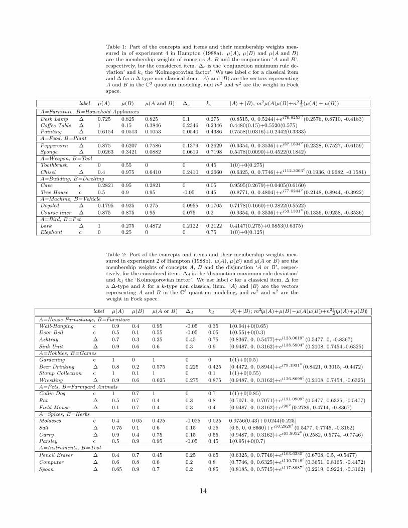
Table 1: Part of the concepts and items and their membership weights mea-sured in of experiment 4 in Hampton (1988a). µ(A), µ(B) and µ(A and B)are the membership weights of concepts A, B and the conjunction ‘A and B’,respectively, for the considered item. ∆c is the ‘conjunction minimum rule de-viation’ and kc the ‘Kolmogorovian factor’. We use label c for a classical itemand ∆ for a ∆-type non classical item. |A〉 and |B〉 are the vectors representingA and B in the C3 quantum modeling, and m2 and n2 are the weight in Fockspace.

label µ(A) µ(B) µ(A and B) ∆c kc |A〉+ |B〉; m2µ(A)µ(B)+n2 12

(µ(A) + µ(B))

A=Furniture, B=Household Appliances

Desk Lamp ∆ 0.725 0.825 0.825 0.1 0.275 (0.8515, 0, 0.5244)+ei76.8253(0.2576, 0.8710, -0.4183)

Coffee Table ∆ 1 0.15 0.3846 0.2346 0.2346 0.4480(0.15)+0.5520(0.575)Painting ∆ 0.6154 0.0513 0.1053 0.0540 0.4386 0.7558(0.0316)+0.2442(0.3333)A=Food, B=Plant

Peppercorn ∆ 0.875 0.6207 0.7586 0.1379 0.2629 (0.9354, 0, 0.3536)+ei87.1634(0.2328, 0.7527, -0.6159)

Sponge ∆ 0.0263 0.3421 0.0882 0.0619 0.7198 0.5478(0.0090)+0.4522(0.1842)A=Weapon, B=ToolToothbrush c 0 0.55 0 0 0.45 1(0)+0(0.275)

Chisel ∆ 0.4 0.975 0.6410 0.2410 0.2660 (0.6325, 0, 0.7746)+ei112.3003(0.1936, 0.9682, -0.1581)

A=Building, B=DwellingCave c 0.2821 0.95 0.2821 0 0.05 0.9595(0.2679)+0.0405(0.6160)

Tree House c 0.5 0.9 0.95 -0.05 0.45 (0.8771, 0, 0.4804)+ei77.0244(0.2148, 0.8944, -0.3922)

A=Machine, B=VehicleDogsled ∆ 0.1795 0.925 0.275 0.0955 0.1705 0.7178(0.1660)+0.2822(0.5522)

Course liner ∆ 0.875 0.875 0.95 0.075 0.2 (0.9354, 0, 0.3536)+ei53.1301(0.1336, 0.9258, -0.3536)

A=Bird, B=PetLark ∆ 1 0.275 0.4872 0.2122 0.2122 0.4147(0.275)+0.5853(0.6375)Elephant c 0 0.25 0 0 0.75 1(0)+0(0.125)

Table 2: Part of the concepts and items and their membership weights mea-sured in experiment 2 of Hampton (1988b). µ(A), µ(B) and µ(A or B) are themembership weights of concepts A, B and the disjunction ‘A or B’, respec-tively, for the considered item. ∆d is the ‘disjunction maximum rule deviation’and kd the ‘Kolmogorovian factor’. We use label c for a classical item, ∆ fora ∆-type and k for a k-type non classical item. |A〉 and |B〉 are the vectorsrepresenting A and B in the C3 quantum modeling, and m2 and n2 are theweight in Fock space.

label µ(A) µ(B) µ(A or B) ∆d kd |A〉+|B〉; m2(µ(A)+µ(B)−µ(A)µ(B))+n212

(µ(A)+µ(B))

A=House Furnishings, B=FurnitureWall-Hanging c 0.9 0.4 0.95 -0.05 0.35 1(0.94)+0(0.65)Door Bell c 0.5 0.1 0.55 -0.05 0.05 1(0.55)+0(0.3)

Ashtray ∆ 0.7 0.3 0.25 0.45 0.75 (0.8367, 0, 0.5477)+ei123.0619(0.5477, 0, -0.8367)

Sink Unit ∆ 0.9 0.6 0.6 0.3 0.9 (0.9487, 0, 0.3162)+ei138.5904(0.2108, 0.7454,-0.6325)

A=Hobbies, B=GamesGardening c 1 0 1 0 0 1(1)+0(0.5)

Beer Drinking ∆ 0.8 0.2 0.575 0.225 0.425 (0.4472, 0, 0.8944)+ei79.1931(0.8421, 0.3015, -0.4472)

Stamp Collection c 1 0.1 1 0 0.1 1(1)+0(0.55)

Wrestling ∆ 0.9 0.6 0.625 0.275 0.875 (0.9487, 0, 0.3162)+ei126.8699(0.2108, 0.7454, -0.6325)

A=Pets, B=Farmyard AnimalsCollie Dog c 1 0.7 1 0 0.7 1(1)+0(0.85)

Rat ∆ 0.5 0.7 0.4 0.3 0.8 (0.7071, 0, 0.7071)+ei121.0909(0.5477, 0.6325, -0.5477)

Field Mouse ∆ 0.1 0.7 0.4 0.3 0.4 (0.9487, 0, 0.3162)+ei90(0.2789, 0.4714, -0.8367)

A=Spices, B=HerbsMolasses c 0.4 0.05 0.425 -0.025 0.025 0.9756(0.43)+0.0244(0.225)

Salt ∆ 0.75 0.1 0.6 0.15 0.25 (0.5, 0, 0.8660)+ei50.2820(0.5477, 0.7746, -0.3162)

Curry ∆ 0.9 0.4 0.75 0.15 0.55 (0.9487, 0, 0.3162)+ei65.9052(0.2582, 0.5774, -0.7746)

Parsley c 0.5 0.9 0.95 -0.05 0.45 1(0.95)+0(0.7)A=Instruments, B=Tool

Pencil Eraser ∆ 0.4 0.7 0.45 0.25 0.65 (0.6325, 0, 0.7746)+ei103.6330(0.6708, 0.5, -0.5477)

Computer ∆ 0.6 0.8 0.6 0.2 0.8 (0.7746, 0, 0.6325)+ei110.7048(0.3651, 0.8165, -0.4472)

Spoon ∆ 0.65 0.9 0.7 0.2 0.85 (0.8185, 0, 0.5745)+ei117.8987(0.2219, 0.9224, -0.3162)

14

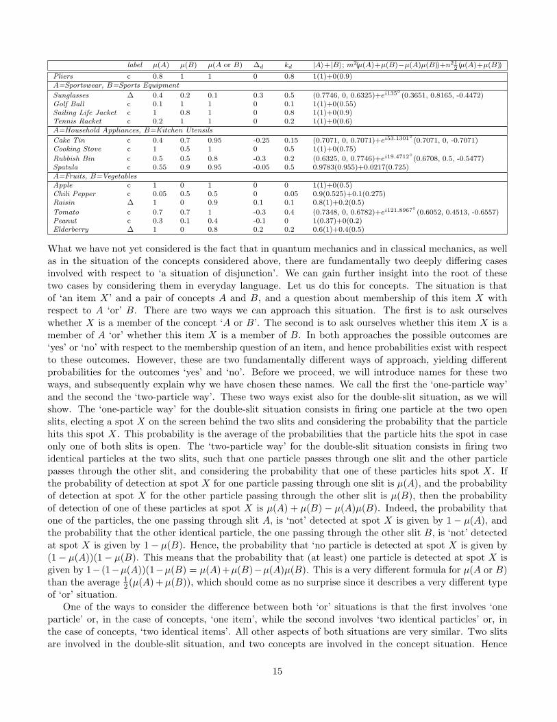
label µ(A) µ(B) µ(A or B) ∆d kd |A〉+|B〉; m2(µ(A)+µ(B)−µ(A)µ(B))+n212

(µ(A)+µ(B))

Pliers c 0.8 1 1 0 0.8 1(1)+0(0.9)A=Sportswear, B=Sports Equipment

Sunglasses ∆ 0.4 0.2 0.1 0.3 0.5 (0.7746, 0, 0.6325)+ei135(0.3651, 0.8165, -0.4472)

Golf Ball c 0.1 1 1 0 0.1 1(1)+0(0.55)Sailing Life Jacket c 1 0.8 1 0 0.8 1(1)+0(0.9)Tennis Racket c 0.2 1 1 0 0.2 1(1)+0(0.6)A=Household Appliances, B=Kitchen Utensils

Cake Tin c 0.4 0.7 0.95 -0.25 0.15 (0.7071, 0, 0.7071)+ei53.1301(0.7071, 0, -0.7071)

Cooking Stove c 1 0.5 1 0 0.5 1(1)+0(0.75)

Rubbish Bin c 0.5 0.5 0.8 -0.3 0.2 (0.6325, 0, 0.7746)+ei19.4712(0.6708, 0.5, -0.5477)

Spatula c 0.55 0.9 0.95 -0.05 0.5 0.9783(0.955)+0.0217(0.725)A=Fruits, B=VegetablesApple c 1 0 1 0 0 1(1)+0(0.5)Chili Pepper c 0.05 0.5 0.5 0 0.05 0.9(0.525)+0.1(0.275)Raisin ∆ 1 0 0.9 0.1 0.1 0.8(1)+0.2(0.5)

Tomato c 0.7 0.7 1 -0.3 0.4 (0.7348, 0, 0.6782)+ei121.8967(0.6052, 0.4513, -0.6557)

Peanut c 0.3 0.1 0.4 -0.1 0 1(0.37)+0(0.2)Elderberry ∆ 1 0 0.8 0.2 0.2 0.6(1)+0.4(0.5)

What we have not yet considered is the fact that in quantum mechanics and in classical mechanics, as wellas in the situation of the concepts considered above, there are fundamentally two deeply differing casesinvolved with respect to ‘a situation of disjunction’. We can gain further insight into the root of thesetwo cases by considering them in everyday language. Let us do this for concepts. The situation is thatof ‘an item X’ and a pair of concepts A and B, and a question about membership of this item X withrespect to A ‘or’ B. There are two ways we can approach this situation. The first is to ask ourselveswhether X is a member of the concept ‘A or B’. The second is to ask ourselves whether this item X is amember of A ‘or’ whether this item X is a member of B. In both approaches the possible outcomes are‘yes’ or ‘no’ with respect to the membership question of an item, and hence probabilities exist with respectto these outcomes. However, these are two fundamentally different ways of approach, yielding differentprobabilities for the outcomes ‘yes’ and ‘no’. Before we proceed, we will introduce names for these twoways, and subsequently explain why we have chosen these names. We call the first the ‘one-particle way’and the second the ‘two-particle way’. These two ways exist also for the double-slit situation, as we willshow. The ‘one-particle way’ for the double-slit situation consists in firing one particle at the two openslits, electing a spot X on the screen behind the two slits and considering the probability that the particlehits this spot X. This probability is the average of the probabilities that the particle hits the spot in caseonly one of both slits is open. The ‘two-particle way’ for the double-slit situation consists in firing twoidentical particles at the two slits, such that one particle passes through one slit and the other particlepasses through the other slit, and considering the probability that one of these particles hits spot X. Ifthe probability of detection at spot X for one particle passing through one slit is µ(A), and the probabilityof detection at spot X for the other particle passing through the other slit is µ(B), then the probabilityof detection of one of these particles at spot X is µ(A) + µ(B) − µ(A)µ(B). Indeed, the probability thatone of the particles, the one passing through slit A, is ‘not’ detected at spot X is given by 1− µ(A), andthe probability that the other identical particle, the one passing through the other slit B, is ‘not’ detectedat spot X is given by 1− µ(B). Hence, the probability that ‘no particle is detected at spot X is given by(1− µ(A))(1− µ(B). This means that the probability that (at least) one particle is detected at spot X isgiven by 1− (1−µ(A))(1−µ(B) = µ(A)+µ(B)−µ(A)µ(B). This is a very different formula for µ(A or B)than the average 1

2(µ(A) +µ(B)), which should come as no surprise since it describes a very different typeof ‘or’ situation.

One of the ways to consider the difference between both ‘or’ situations is that the first involves ‘oneparticle’ or, in the case of concepts, ‘one item’, while the second involves ‘two identical particles’ or, inthe case of concepts, ‘two identical items’. All other aspects of both situations are very similar. Two slitsare involved in the double-slit situation, and two concepts are involved in the concept situation. Hence

15

the difference is determined by what happens with the particles in passing through the slits. Either thereis one particle passing through one of both slits or there are two identical particles such that each passesthrough one of the slits. Although structurally identical, the difference is a lot more subtle in the case ofconcepts. Indeed, for the double-slit and the ‘one-particle way’ or the ‘two-particle way’, one can, anyhowif it is about classical particles, distinguish, in the sense that in one case there is only one particle involved,while in the other case there are two particles involved. In the concept situation, ‘one item’ is involvedin the case of the ‘one-particle way’ and ‘two identical items’ are involved in the case of the ‘two-particleway’. To identify this difference within a human thought-process is much more complicated, however, alsosince ‘the making of an identical item starting from a considered item within human thought is a processtaking place all the time’.

Let us consider the concrete situation of a subject participating in one of the experiments describedin Hampton (1988b). We can reflect intuitively on the ‘human thought process’ taking place in his or hermind and imagine that both ways can take place. We will illustrate this by means of an example. Supposea subject is asked to answer with ‘yes’ or ‘no’ the question whether Almond is a member of Fruits orVegetables. Following only the first way – the ‘one-particle way’ –, the subject would consider ‘Fruits orVegetables’ a wholly new concept and answer the question of whether or not Almond is a member of thisnew concept ‘Fruits or Vegetable’. Following only the second way – the ‘two-particle way’ –, the subjectwould consider two identical items Almond in turn, deciding for the one whether it is a member of Fruitsand for the other whether it is a member of Vegetables. While doing so the subject makes a complicatedconfrontation of these two decision possibilities with the notion of ‘or’ in the background and decides in thisway about ‘yes’ or ‘no’ with respect to membership for the item Almond. This complicated confrontationis what has been organized in truth tables by logicians within their discipline called ‘logic’, because indeedit comes to deciding ‘yes’ for membership in case ‘yes, yes’, ‘yes, no’ or ‘no, yes’ would have been decidedfor membership with respect to the concepts apart.

What Hampton (1988b) experiments show is that ‘both ways take place’. After carefully analyzingthe experimental data, which we will do in subsection 1.7, we conclude that these two ways occur insuperposition. The ‘superposition’ of both ways, the one-particle way and the two-particle way, is exactlywhat quantum-fields theory offers to meet our modeling need, and the mathematical space it uses for thisis Fock space. That is why in Aerts (2007a,b) we elaborated a Fock space model for the disjunction of twoconcepts.

The following examples taken from the Hampton experiments further illustrate the mechanism thatwe propose here. They also serve to help explain what we mean by our hypothesis that ‘human thoughtcomprises two superposed layers’. Let us consider the item Apple with respect to the pair of concepts Fruitsand Vegetables and their disjunction Fruits or Vegetables. A subject following the ‘two-particle way’ will goabout answering the question more or less as follows: “An apple is certainly a fruit and it is definitely nota vegetable”. In this part of the thought process, the subject splits up the item Apple into two identicalitems, confronting them with the concepts Fruits or Vegetables, respectively. The subject’s thought processthen continues: “But since it is a fruit, it must necessarily also be a ‘fruit or a vegetable’”. In this partof the thought process, the subject follows a logical line of reasoning, combining the two confrontationswith the concepts. Let us now suppose that he the subject follows the ‘one-particle way’ for resolving theApple and ‘Fruits or Vegetables’ question. In this case, the subject would consider ‘Fruits or Vegetables’to be a wholly new concept and determine whether or not Apple is a member of this new concept. Applebeing a very archetypical Fruit, it is very unlikely for the subject to regard Apple as a strong member ofthe new Fruit or Vegetable concept, because this is an overall concept for all items belonging to Fruits orVegetables. In other words, while in this situation the ‘two-particle way’ should yield µ(A or B) = 1 forthis situation, the ‘one-particle way’ should yield µ(A or B) = 1

2 . The experiments described in Hampton(1988b) concerning Apple with respect to Fruits, Vegetables and Fruits or Vegetables give membership

16

weights µ(A) = 1, µ(B) = 0 and µ(A or B) = 1. This shows that this particular comparison betweenApple and ‘Fruits or Vegetables’ is very much dominated by the two-particle way.

Let us now return to the example of Almond. The experimental data about membership weightsof Almond with respect to the pair of concepts Fruits and Vegetables and their disjunction describedin Hampton (1988b) are µ(A) = 0.2, µ(B) = 0.1 and µ(A or B) = 0.425, respectively. Hence kd =µ(A) + µ(B) − µ(A or B) = −0.125 ≤ 0, which shows that Almond is a k-type non-classical item. Wecan see that, for Almond, the second way, the ‘one-particle way’, is strongly dominant. While Almond wasassigned hardly any weight as a member of both Fruits and Vegetables, it was assigned considerable weightas a member ‘Fruits or Vegetables’. Apparently, Almond was regarded as one of those items that raisedoubts as to whether they are Fruits or Vegetables, neither of the two categories offering a satisfactorytypification individually. This makes it a fairly good member of the new concept ‘Fruits or Vegetables’.

Analogous to ‘one-particle way’ and ‘two-particle way’, we will use the terms ‘one train of thought way’and ‘two trains of thought way’ in dealing with concepts. Indeed, one can imagine the ‘two-particle way’ astwo parallel trains of thought taking place in the subject’s mind. One train of thought is aimed at decidingabout the membership of item X with respect to concept A and the second train of thought is aimed atdeciding about the membership weight of item X with respect to concept B. The two trains of thoughttake place in parallel, and either of them confirming membership of item X with respect to one of theconcepts, say concept A, is sufficient for membership of item X with respect to ‘A or B’ to be confirmedas well. Once one of the trains of thought has established membership, the outcome of the other trainof thought has become irrelevant. Only if both trains of thought deny membership with respect to bothconcepts, will membership with respect to the disjunction be denied as well. Since this way of reasoning isin line with classical logic with respect to the disjunction of two propositions, we have called it the ‘classicallogical way’. If this is the ‘only’ way of reasoning in the subject’s mind, the data will come out as classicaldata, i.e. data that can be modeled within a classical measure or probability structure. An item for whichthe ‘classical logical’ way is very dominant will experimentally show itself as what we have called a classicalitem. Apple with respect to Fruits, Vegetables and ‘Fruits or vegetables’ is such an example. What we havecalled the ‘one-particle way’ or ‘one train of thought way’ introduces a way of thought that is very differentfrom this classical logical thought. We will call it ‘quantum conceptual thought’. A subject who followsonly the quantum conceptual thought way, focuses on one and only one train of thought with respect to‘A or B’, and hence directly wonders whether the item X is a member or not a member of ‘A or B’. In‘quantum conceptual thought’ the subject considers A or B as a new concept, hence the emergence ofthe concept ‘A or B’. Quantum mechanics as a mathematical formalism is suited to describe ‘quantumconceptual thought’ since the mathematical operation of ‘superposition’ produces a ‘new state with newfeatures’, and classical theories do not entail such a possibility.

The distinction of two modes of thought has been proposed by many and in many different ways.Sigmund Freud, in his seminal work ‘The interpretation of dreams’, already proposed to consider thoughtas consisting of two processes, which he called primary and secondary (Freud, 1899) and were to becomepopularly known as the conscious and the subconscious. William James subsequently introduced the idea of‘two legs of thought’, specifying the one as ‘conceptual’, i.e. exclusive, static, classical and following the rulesof logic, and the other as ‘perceptual’, i.e. intuitive and penetrating. He expressed the opinion that ‘justas we need two legs to walk, we also need both conceptual and perceptual modes to think’ (James, 1910).More recently, Jerome Bruner introduced the ‘paradigmatic mode of thought’, transcending particularitiesto achieve systematic categorical cognition where propositions are linked by logical operators, and the‘narrative mode thought’, engaging in sequential, action-oriented, detail-driven thought, where thinkingtakes the form of stories and ‘gripping drama’ (Bruner, 1990). Aspects of different modes of thoughtand the influence of their presence on human cognitive evolution were also proposed in Gabora and Aerts(2009). Another point that we think is relevant to our structure of two superposed layers – subsection 1.8

17

explains why – is how Tversky & Kahneman (1982) introduced the notion of ‘representative heuristic’ todescribe the decision process that lies at the basis of what happens during ‘disjunction effect situations’ or‘conjunction fallacy situations’ and other similar situations. We believe that all these examples, and others,are related but also different from the superposed layers we introduce in this paper. We intend to dedicatefuture research to these relations and differences, continuing along the lines of Aerts and D’Hooghe (2009).

1.7 Fock Space and What About Conjunction

As said, our general scheme makes use, next to ‘superposition’ and ‘interference’, of a ‘quantum field theo-retic aspect’. In quantum field theory the entity that is described, i.e. the field, consists of superpositionsof different configurations of many quantum particles. This is why the mathematical space used to describethis quantum field is a Fock space, which is a direct sum – this is the superposition part – of differentHilbert spaces, where each Hilbert space represents a certain number of quantum particles. In the casewhere we consider two concepts A and B, a field theoretic model consists of the direct sum of two Hilbertspaces. One Hilbert space H describes the ‘one-particle situation’, i.e. the situation where ‘A or B’ isconsidered to be a new concept, and its state in this Hilbert space is 1√

2(|A〉+ |B〉), while the experiment

to determine membership of an item X is described by the orthogonal projection M . It is the descriptionthat we have presented in section 1.5.

A second Hilbert space describes the ‘two-particle way’, which is the tensor product H⊗H. The stateof the concepts A and B is represented by a vector |A〉 ⊗ |B〉 of this tensor product Hilbert space. Toknow how to describe the ‘decision measurement’ for this ‘two-particle way’ quantum-mechanically, let usanalyze in detail the decision process. We will do this by modeling the situation where a subject is askedto decide on the membership of an item X with respect to concept ‘A or B’. To answer this question,the subject will consider ‘two identical items X’, pondering on the membership of one of the two identicalitems X with respect to A ‘and’ the membership of the other one of the two identical items X with respectto B. The outcome will therefore be one of the following answers: (i) ‘yes, yes’, which means that thesubject decides that one of the items X is a member of A and the other identical item X is a memberof B; (ii) ‘yes, no’, which means that the subject decides that one of the items X is not a member of Aand the other is a member of B; (iii) ‘no, yes’, which means that the subject decides that one of the itemsX is not a member of A and the other is a member of B; and finally (iv) ‘no, no’, which means that thesubject decides that one of the items X is not a member of A and the other item X is not a member of B.The subject will affirm membership of X with respect to ‘A or B’ if the outcome is ‘yes, yes’, ‘yes, no’ or‘no, yes’. The decision experiment with respect to membership of item X is described by the orthogonalprojection M ⊗M , which is a linear operator on the tensor product Hilbert space H ⊗H. Following theabove analysis, membership weight for the disjunction is given by

µ(A or B) = 1− (〈A| ⊗ 〈B|)(1−M)⊗ (1−M)|(|A〉 ⊗ |B〉) (18)

where indeed a ‘yes’ for the disjunction means that one of the outcomes ‘yes, yes’, ‘yes, no’ or ‘no, yes’ isobtained, which is equivalent to the outcome ‘no, no’ not being obtained.

In sections 1.5 and 1.6 we discussed the disjunction of two concepts A and B at great length. We willnow look at the conjunction of two concepts A and B. Now that we have understood that 1√

2(|A〉+ |B〉)

represents a new concept ‘A or B’, and not the logical construction ‘concept A’ or ‘concept B’, it may well bethat with the conjunction also correspond a ‘one-particle way’ and a ‘two-particle way’. There is yet anotherfact that points to this. Note, for example, that ‘underextension’, which is the commonest effect measuredby Hampton (1988b) for disjunction, produces a value for µ(A or B) that deviates from max(µ(A), µ(B))‘in the direction of the average 1

2(µ(A)+µ(B))’. More specifically, the average 12(µ(A)+µ(B)) is in general

‘underextended’ itself. Overextension, which is the commonest effect measured by Hampton (1988a) for

18

conjunction, produces a value for µ(A and B) that deviates from min(µ(A), µ(B)) ‘also in the directionof the average 1

2(µ(A) + µ(B))’. And the average 12(µ(A) + µ(B)) is in general ‘overextended’ itself. This

suggests that ‘underextension for the disjunction’ and ‘overextension for the conjunction’ could well becaused by the same effect. And indeed, in our explanatory scheme, they are caused by the same effect,namely by the effect of the presence of the emergence of a new concept. In the case of the conjunction,this is the concept ‘A and B’. We can now explain how we have modeled the conjunction data in Table1, i.e. using the same quantum description, for example the one worked out in C3 for the disjunction. Werefer to Aerts (2007b) for a detailed elaboration of this modeling.

Finally we have all the material to explain the modeling in Fock space, and, therefore, the motivationfor the simple quantum model presented in section 2. Fock space F is the direct sum of both Hilbert spaces,the ‘two-particle way’ Hilbert space and the ‘one-particle way’ Hilbert space, hence F = (H⊗H)⊕H, andthe state ψ(A,B) of the concepts A and B in Fock space is described by a normalized linear combinationof the ‘two-particle state’ and the ‘one-particle state’. Concretely, this leads to

ψ(A,B) = meiθ|A〉 ⊗ |B〉+neiφ√

2(|A〉+ |B〉) m2 + n2 = 1 (19)

The experiment testing whether an item X ‘is’ or ‘is not’ a member of the concept ‘A and B’ is describedby the projection operator M ⊗M ⊕M working on this Fock space. The probability that the outcome is‘yes’, i.e. that a subject decides in favor of membership of the item X with respect to the concept ‘A andB’, is given by

µ(A and B) = (meiθ〈A| ⊗ 〈B|+ neiφ√2

(〈A|+ 〈B|))M ⊗M ⊕M(meiθ|A〉 ⊗ |B〉+neiφ√

2(|A〉+ |B〉))(20)

= m2(〈A| ⊗ 〈B|)M ⊗M |(|A〉 ⊗ |B〉) +n2

2(〈A|+ 〈B|)M(|A〉+ |B〉) (21)

= m2〈A|M |A〉〈B|M |B〉+n2

2(〈A|M |A〉+ 〈B|M |B〉+ 〈A|M |B〉+ 〈B|M |A〉) (22)

= m2µ(A)µ(B) + n2(µ(A) + µ(B)

2+ <〈A|M |B〉) (23)

Let us mention that our quantum modeling of the conjunction differs from the quantum model of theconjunction presented by Franco (2007), in that he employs conditional probability and we make use ofhow the conjunction appears in Fock space. Let us construct the Fock space probability for the disjunctionnow.

The probability µ(A or B) that a subject decides in favor of membership of the item X with respectto the concept ‘A or B’ is given by 1 minus the probability of a decision against membership of the itemX with respect to the concept ‘A and B’. This means that

µ(A or B) = 1−m2(1− µ(A))(1− µ(B)− n2(1− µ(A) + 1− µ(B)

2+ <〈A|1−M |B〉) (24)

= m2 + n2 −m2(1− µ(A)− µ(B) + µ(A)µ(B))− n2(2− µ(A)− µ(B)

2−<〈A|M |B〉)(25)

= m2(µ(A) + µ(B)− µ(A)µ(B)) + n2(µ(A) + µ(B)

2+ <〈A|M |B〉) (26)

By means of equations (23) and (26) we can show how the experimental data of Hampton (1988a,b)make a strong case for the introduction of Fock space as a generalization of a single Hilbert space. Forexample, consider the item Cave with respect to the pair of concepts Building and Dwelling and theirconjunction Building and Dwelling. As we can see in Table 1, we have µ(A) = 0.2821 and µ(B) = 0.95

19

and µ(A and B) = 0.2821, which shows that Cave is a classical item. But it cannot be modeled by meansof quantum interference only, i.e. in the ‘one-particle way’. We can understand why quantum interferencealone cannot model Cave. The ‘one-particle way’ produces deviations from the average 1

2(µ(A) + µ(B))due to interference. However, if one of the weights µ(A) or µ(B) is close to zero, and the other is closeto 1, like in the case of Cave, the average is a number far removed from µ(A) and from µ(B). The sizeof the interference is proportional to the smallest term of

√µ(A)µ(B) or

√(1− µ(A))(1− µ(B), which

means that interference is small if µ(A) and µ(B) are close to 0 or 1. If then additionally µ(A and B)is close to 0 or 1, the value of µ(A and B) will not be reached by adding or subtracting the interferencefrom the average. This is what happens for Cave where µ(A) and µ(A and B) are both close to zero, andµ(B) is close to 1. If the item is classical, and one of the weights is close to zero and the other is close to1, the weight of the conjunction will be close to the smallest of µ(A) and µ(B), resulting in the situationwhich does not allow modeling by quantum interference. Table 1 gives examples of items in this situationfor the conjunction, more specifically Coffee Table and Painting for to the pair of concepts Furniture andHousehold Appliances; Sponge for the pair of concepts Food and Plant; Toothbrush for the pair of conceptsWeapon and Tool; Cave for the pair of concepts Building and Dwelling; Dogsled for the pair of conceptsMachine and Vehicle and Lark and Elephant for the pair of concepts Bird and Pet, and Table 2 shows alist of items where for the disjunction no quantum model with only interference exist, more specificallyWall-Hanging and Door Bell for the pair of concepts House Furnishings and Furniture; Gardening andStamp Collection for the pair of concepts Hobbies and Games; Collie Dog for the pair of concepts Pets andFarmyard Animals; Molasses and Parsley for the pair of concepts Spices and Herbs; Pliers for the pair ofconcepts Instruments and Tools; Golf Ball, Sailing Life Jacket and Tennis Racket for the pair of conceptsSportswear and Sports Equipment; Cooking Stove and Spatula for the pair of concepts Household AppliancesandKitchen Utensils; Apple, Chili Pepper, Raisin, Peanut and Elderberry for the pair of concepts Fruitsand Vegetables. The others items in Table 1 and Table 2 are presented there as quantum modeled withinterference alone by making use of the C3 model of section 1.5.

The items that don’t allow a quantum model with interference alone can usually be modeled in Fockspace with equations (23) and (26) for conjunction and disjunction. For example, consider equation (23)and suppose that we neglect the interference term. Then we have µ(A and B) = m2µ(A)µ(B)+n2 1

2(µ(A)+µ(B)), which is the convex combination of the product and the average of both weights µ(A) and µ(B).Table 1 shows how each one of the items that cannot be modeled by quantum interference alone for theconjunction can be modeled in Fock space, and it gives the convex weights m2 and n2 for each item. Inan analogous way, we show how the items that cannot be modeled by quantum interference alone for thedisjunction are modeled in Fock space by giving the value of the convex weights m2 and n2 using equation(26) with zero interference. This allows us to put forward the following statement.

Motivation for Fock space: Classical items with one of their weights close to 0 and the other closeto 1 cannot in general be modeled by a quantum model where only quantum interference is introduced asquantum effect. They can usually be modeled in Fock space.

1.8 Application to Decision Theory, Economics and Other Domains

In this section we will analyze the relevance of the general quantum modeling scheme to decision theoryand economics, explaining how our hypothesis of the superposed layered structure of classical logical andquantum conceptual thought can shed light on situations there. Next to the modeling within our quantummodeling scheme, we will also suggest, and attempt to prove, that our concept analysis can help explainthe effects that we will consider in these domains. We will also mention other domains of science where wehave identified connections and analogies, such as semantic analysis and artificial intelligence, and pointout domains where other scientists have applied quantum structures.

20

The disjunction effect in decision theory is an example of a situation that can be described in ourgeneral quantum modeling scheme (Tversky & Shafir,1992). This effect, in its game theoretic version, hasalready been modeled successfully within a quantum game theoretic scheme in Busemeyer, Matthew andWang (2006). Let us shortly describe how it is modeled within our scheme. The disjunction effect occurswhen test subjects prefer option x (to y) if they know that both event A and event B will occur (usuallyB is taken to be not A, but that is not essential), but refuse option x (or prefer option y) if they knowneither whether A will occur nor whether B will occur. The best-known example of this disjunction effectis the so-called Hawaii problem, which also originated its analysis, and which is about the following twosituations (Tversky & Shafir,1992).

Disjunctive version: Imagine that you have just taken a tough qualifying examination. It is the end ofthe fall quarter, you feel tired and run-down, and you are not sure that you passed the exam. In case youfailed you have to take the exam again in a couple of months after the Christmas holidays. You now havean opportunity to buy a very attractive 5-day Christmas vacation package to Hawaii at an exceptionallylow price. The special offer expires tomorrow, while the exam grade will not be available until the followingday. Would you: x buy the vacation package; y not buy the vacation package; z pay a $5 non-refundablefee in order to retain the rights to buy the vacation package at the same exceptional price the day aftertomorrow after you find out whether or not you passed the exam.

Pass/fail version: Imagine that you have just taken a tough qualifying examination. It is the endof the fall quarter, you feel tired and run-down, and you find out that you passed the exam (failed theexam. You will have to take it again in a couple of month after the Christmas holidays). You now have anopportunity to buy a very attractive 5-day Christmas vacation package to Hawaii at an exceptionally lowprice. The special offer expires tomorrow. Would you: x buy the vacation package; y not buy the vacationpackage: z pay a $5 non-refundable fee in order to retain the rights to buy the vacation package at thesame exceptional price the day after tomorrow.

In the Hawaii problem, more than half of the subjects chose option x (buy the vacation package) if theyknew the outcome of the exam (54% in the pass condition and 57% in the fail condition), but only 32% didso if they did not know the outcome of the exam. Let us explicitly construct the quantum model for theHawaii problem, and use the C3 realization that we introduced in subsection 1.5. The states |A〉 and |B〉 ofthe Hilbert space now represent situation A, ‘having passed the exam’, and situation B, ‘not having passedthe exam’. The decision to be taken is ‘to buy the vacation package’ or ‘not buy the vacation package’.This decision is described in the Hilbert space by means of projection operator M . The probability for anoutcome ‘yes’ (buy the package) in the ‘pass’ situation (state |A〉) is 0.54, i.e. in our notation µ(A) = 0.54.The probability for an outcome ‘yes’ (buy the package) in the ‘fail’ situation (state |B〉) is 0.57, i.e. in ournotation µ(B) = 0.57. The probability for an outcome ‘yes’ (buy the package) in the ‘outcome unknown’situation (state 1√

2(|A〉 + |B〉)) is 0.32, i.e. in our notation µ(A or B) = 0.32. Applying the C3 model

introduced in 1.5, we have to verify first whether µ(A) + µ(B) = 1.11 is smaller or greater than 1, andsince it is greater, we put a = 0.54, b = 0.57 and apply equations (15), (16) and (17) to find

|A〉 = (0.7348, 0, 0.6782) |B〉 = eiβ(0.6052, 0.4513,−0.6557) β = 121.8967 (27)

which completes the C3 quantum model. We can indeed verify that, using these values for |A〉, |B〉 and θ,and choosing M(C3) as the plane spanned by (1, 0, 0) and (0, 1, 0), i.e. M being the orthogonal projectoron this plane, we get

µ(A) = 〈A|M |A〉 = (0.7348)2 = 0.54 (28)µ(B) = 〈B|M |B〉 = e−iβeiβ((0.6052)2 + (0.4513)2) = (0.6052)2 + (0.4513)2 = 0.57 (29)

µ(A or B) =12

(〈A|+ 〈B|)M(|A〉+ |B〉) =12

(µ(A) + µ(B)) + 〈A|M |B〉+ 〈B|M |A〉) (30)

21

=12

(0.54 + 0.57 + (0.7348)(0.6052)ei121.8967 + (0.6052)(0.7348)e−i121.8967) (31)

= 0.555 + 0.4447 cos 121.8967 = 0.555− 0.235 = 0.32 (32)

which are the values found experimentally in the Hawaii experiment.Our quantum modeling scheme enables us to explain this Hawaii problem as follows. The whole

landscape of concepts and their combinations play a role in determining the weights that are connectedwith the decision process. If we would model this conceptual landscape within Fock space, we would beable to calculate the weights as predicted by quantum calculation in Fock space. Of course, constructingthe Fock space states of this conceptual landscape requires carrying out a large number of experiments toanalyze the situation and gather sufficient knowledge on the preparation of such states. To illustrate this,let us suppose that the Hawaii dilemma is not about buying or not buying a vacation package but aboutsaying yes or no to a free Sauna and Jacuzzi relaxation weekend. In this case, the outcome may well bethe opposite, with a larger than expected number of subjects saying yes even without knowing their examresults. We believe that in the Hawaii situation, the underextension is due to the fact that the idea ofmaking a trip is appealing only if the outcome of the results is known, whether pass or fail, whereas a freerelaxation weekend is much more likely to be appealing even if the exam results have not been released yet.This situation is very similar to, for example, Almond being an overextended item with respect to Fruitsor Vegetables, because it fits well with the uncertainty ‘whether it is a Fruit or a Vegetable’. This kind ofreflections is discussed in greater detail in Aerts and D’Hooghe (2009).

Busemeyer, Matthew and Wang (2006) model the game theoretic variant of the disjunction effecton a quantum game theoretic model, and, in a very interesting way, use the Schrodinger equation todescribe the dynamics of the decision process. Their model is part of a general operational approach ofcomparing classical stochastic models with quantum dynamic models, and deciding by comparison withexperimental data which of both models has most predictive power (Busemeyer, Wang & Townsend, 2006).Also Andrei Khrennikov has presented a quantum model for decision making (Khrennikov, 2008). By meansof an algorithm probabilistic data of any origin are represented by complex probability amplitudes. Thealgorithm is used to model the Prisoners Dilemma and the disjunction effect.

The model of the Hawaii situation which we present here is very similar – at least with regard to thestructure of state space, i.e. Hilbert space – to what can be found in Busemeyer, Matthew and Wang(2006) and in Khrennikov (20080, since we use here only the ‘one-particle way’. The situation changes,however, if we add the ‘two-particle way’ for the disjunction, working in Fock space, like we did for our‘disjunction of concepts model’ in Aerts (2007a,b) and in the present article. Detailed testing with manydifferent alternatives in choice for the ‘disjunction effect experimental situation’ is necessary to find outwhether a Fock space model is needed. If the type of explanation for the effect that we put forward here,namely that the whole conceptual landscape plays a role, is correct, most probably a Fock space modelwill be needed to complement the single Hilbert space model if different experimental data pertaining tothe same disjunction effect situation are attempted to be modeled. There are some recent experiments onthe disjunction effect that point in this direction (Bagassi & Macchi, 2007), and we have analyzed them insome detail in Aerts and D’Hooghe (2009).

Economics is another domain of science where we can identify situations involving effects that can bedescribed using our quantum modeling scheme. Here are some examples. One of the basic principles ofeconomics, playing a fundamental role in the von Neumann-Morgenstern theory, for instance, is Savage’s‘sure thing principle’ (Savage, 1944). Savage introduced this principle in the following story: A businessmancontemplates buying a certain piece of property. He considers the outcome of the next presidential electionrelevant. So, to clarify the matter to himself, he asks whether he would buy if he knew that the Democraticcandidate were going to win, and decides that he would. Similarly, he considers whether he would buy if heknew that the Republican candidate were going to win, and again finds that he would. Seeing that he would

22

buy in either event, he decides that he should buy, even though he does not know which event obtains, orwill obtain, as we would ordinarily say.

The ‘sure thing principle’ is equivalent to the independence axiom of expected utility theory: ‘inde-pendence’ here means that if a person is indifferent in his or her choice between simple lotteries L1 andL2, he or she will also be indifferent in choosing between L1 mixed with an arbitrary simple lottery L3

with probability p and L2 mixed with L3 with the same probability p. Problems in economics such as theAllais paradox (Allais, 1953) and the Ellsberg paradox (Ellsberg, 1961) show an inconsistency with thepredictions of the expected utility hypothesis, namely a violation of the ‘sure thing principle’.

We can readily identify an item for a pair of concepts measured by Hampton where the ‘sure thingprinciple’ is violated if we would transpose it to the situation of concepts and decision for membership ofitems. For example, let us consider the item Diving Mask with respect to the pair of concepts Sportswearand Sports Equipment and their disjunction Sportswear or Sports Equipment. Hampton (1988b) measuredµ(A) = 1, µ(B) = 1 and µ(A or B) = 0.95. These values for µ(A), µ(B) and µ(A or B) are modeledby our quantum model, the vector is given in Table 3, and equals x = (0.0664, 0, 0, 0, 0.9978, 0, 0, 0), withangles θ = 107 and φ = 12.95. Hence, we can also use our quantum model to model these values if theyare collected experimentally in the situation of the ‘sure thing principle’. More concretely for the situationoriginally proposed by Savage: (i) the businessman will buy the property with certainty if the Democraticcandidate were to win, i.e. µ(A) = 1; (ii) the businessman will buy the property with certainty if theRepublican candidate were to win, i.e. µ(B) = 1; (iii) the businessman will buy the property ‘not’ withcertainty if he does not know the outcome of the elections, i.e. if the situation is such that the Democratic‘or’ the Republican candidate were to win, i.e. µ(A or B) = 0.95. Our quantum model also allows modelingof much lower values than 0.95 for µ(A or B) with µ(A) = µ(B) = 1 for an experimentally tested ‘surething principle situation’ to be modeled.

We have investigated correspondences between our approach and existing cognitive science modelsof knowledge representation. In this way, we were able to prove that modern approaches to semanticanalysis (Deerwester, Dumais & Harshman, 1990; Berry, Dumais & O’Brien, 1995; Lund & Burgess, 1996),if reformulated as Hilbert-space problems, reveal quantum structures similar to those we employ in ourquantum modeling scheme (Aerts and Czachor, 2004), and we have worked out a concrete comparisonwith Latent Semantic Analysis (Landauer, Foltz & Laham, 1998). In Aerts and Czachor (2004), we couldprove a similar correspondence with distributed representations of cognitive structures developed for thepurposes of neural networks (Smolensky, 1990).

After connecting our approach to ongoing semantic analysis and artificial intelligence investigations, wealso looked into its relation with other cognitive science approaches. More specifically, Gardenfors (2004)comes to mind. Although there are certainly interesting connections to point out, and we plan to do soconcretely in future work, there are also quite some differences between the foundations of his approachand ours. We already said that the modeling of linguistic structures is not our primary concern, since wefocus on the semantic content, on the ‘flow and interaction of meaning’. There is, however, something moreto be said on this point. Although modeling, and specifically the modeling of large collections of data, isthe ultimate test for a theory, we must admit that ‘modeling’ is not our primary concern either. Modelingis a necessary and very important test for the theory, but our primary concern is ‘explanation’. Perhapsthis can be better understood by considering our first publication on the subject, Aerts and Aerts (1994).The idea of applying quantum statistics to model a human decision process was then inspired by the factthat in such a decision process the ‘possible outcomes of the decision do not exist prior to the decisionbeing taken’. Classical statistics is a formalization of a situation where these possible outcomes ‘do exist’but ‘we lack knowledge about them’. Quantum statistics is exactly the opposite in this respect, for itdescribes processes where indeterminism appears ‘not due to a lack of knowledge of an already existingset of events’, but ‘due to probability connected to potential (and hence not yet existing) events’. This

23

is the reason and the origin of the quantum decision model we proposed in Aerts and Aerts (1994). Atthis moment, we are still driven by a very similar idea, namely the idea that human decision-making isstructured in a quantum way, not only due to a situation of indeterminism that is not of the ‘lack ofknowledge’ type, but also due to the existence of effects, i.e. overextension, guppy effect, disjunction effect,conjunction fallacy, violation of the Savage ‘sure thing principle’, that are connected with the way we haveconceptually structured our world, by means of concepts and combinations of concepts. We indeed believethat this quantum structure percolates to the realm of ‘how meaning is carried by concepts’. This ideagains considerable plausibility thanks to the fact that the ‘disjunction effect’ and the ‘conjunction fallacy’in decision theory and the violation of Savage’s ‘sure thing principle’ are completely similar effects to the‘underextension’ and ‘overextension’ effects related to disjunction and conjunction in concept combination,and also that concept formation is largely a combinatory process of disjunctions and conjunctions (seesection 4.1).

Returning to Gardenfors (2004), we can say that in his approach the focus is strongly on modeling,and hence a use of geometric structures that is much broader than what our quantum modeling schemehas to offer is possible. In this sense, we feel greater affinity with the attempts to model human thoughtwithin logical structures, started by Aristotle and continued by Boole and numerous logicians after them,except that the quantum Fock space connected structures describe a process of thought that is much morecomplex and where classical logical thought appears as one of the branches of a superposition in Fockspace.

Quantum mechanics has also been used in the domain of information retrieval (Widdows, 2003, 2006;Widdows & Peters, 2003; Van Rijsbergen, 2004), and here it is more specifically the quantum logic structureunderlying quantum mechanics that has proved effective in producing theoretical models for informationretrieval. Widdows and Peters (2003) demonstrated that the use of the quantum logic connective fornegation, i.e. orthogonality, is a powerful tool for exploring and analyzing word meanings that has distinctadvantages over Boolean operators in document retrieval experiments. Van Rijsbergen (2004) introduced ageneral theory for information retrieval based on quantum logic structures. He showed how three keystonemodels used in information retrieval, a vector space model, a probabilistic model and a logical model,can be described in Hilbert space, where a document can be represented by a vector and relevance by aHermitian Operator. Both approaches bear correspondence to our approach.

In the same period of time, the formalization of context effects in relation to concepts and the studyof operational issues related to such effects considering quantum logic was undertaken in Bruza and Cole(2005), inspiring further study of quantum structures in this respect (Bruza, Widdows & Woods (in press)).Another subject that has been investigated is that of quantum structures in language, more specificallythe entanglement of words in human semantic space, resulting in proposals of possible violations of Bellinequalities (Aerts, Czachor & D’Hooghe, 2006; Bruza, Kitto, Nelson & McEvoy, 2008; Bruza, Kitto,Nelson & McEvoy, 2009).

2 A Simple Quantum Model Illustrating the General Scheme

In the foregoing section we have given all elements of our general scheme of quantum modeling to explainwhat is the nature of the simple quantum model that we present in this section. The quantum model wepresent here is constructed in an eight dimensional real vector space R8, consisting of the direct sum of twofour dimensional real vector spaces, hence R8 = R4⊕R4, where the first R4 plays the role of what we havecalled the ‘two particle way’ in the foregoing section. We will show that indeed the ‘classical items’ andthe ‘classical parts of a general item’ can be represented in it. In the second R4 we represent the analogueof the ‘one particle way’ in foregoing section.

What is now the specific value of this model compared to the model elaborated in Aerts (2007a,b)?

24

This model is such that all the items being tested by Hampton with respect to one pair of concepts andits disjunction or conjunction can be modeled giving also a fixed representation to their conjunction anddisjunction. For the standard interference quantum model, the one put forward in Aerts (2007a,b), and inother approaches where quantum mechanics is used in cognition and economy, this is not the case. Morespecifically the superposition vector 1√

2(|A〉 + |B〉), if |A〉 and |B〉 are chosen from specific fixed rays in

Hilbert space, does not necessarily corresponds to one specific ray in Hilbert space, because a lot of differentrays can be reached by choosing different phases for |A〉 and |B〉. This is a well known phenomenon inquantum mechanics and even at the origin of the continuous set of values that is reached by interference.The ‘real vector space model’ presented in the remainder of this article shows that ‘superposition andinterference without complex numbers’ plus all the other aspects of quantum mechanics, is sufficient toproduce a model for the set of cognitive data of Hampton (1988a,b). Such ‘superposition and interferencewithout complex numbers’ allows the representation of the conjunction and disjunction by means of adefinite geometric structure, namely a two dimensional subspace, for each pair of concepts. Next to thisthe model shows in a simple way how the ‘two particle way’ and ‘one particle way’ play out. We believehowever that the model built in Aerts (2007a,b), the one we have presented in section 1.5, will turn outto be the more fundamental one, certainly if it comes to developing a generalized theory for combinationsof large collections of concepts, as put forward in subsection 4.2. In the next subsection we illustrate howthe classical data can be represented in the first R4.

2.1 Quantum Modeling of the Classical Items

We model the classical items in a 4-dimensional vector space over the real numbers, hence R4. We considerthe item Sailboat of the pair of concepts Machine and Vehicle and their conjunction Machine and Vehicleto illustrate the modeling. Subjects attributed membership weights µ(A) = 0.5641, µ(B) = 0.8 andµ(A and B) = 0.4211 respectively with respect to the concepts Machine and Vehicle and their conjunctionMachine and Vehicle. The ‘conjunction minimum rule deviation’ equals -0.1430, and the ‘Kolmogorovianconjunction factor’ equals 0.0570, which makes the item is ‘classical’, following our analysis of section 1.3.We need to specify (i) how we will represent the concepts A, B and their conjunction ‘A and B’; (ii) howwe will represent the item X; and (iii) what are the quantum rules for calculating the weights.

Consider the canonical orthonormal base eAB, eAB′ , eA′B, eA′B′ where eAB = (1, 0, 0, 0), eAB′ =(0, 1, 0, 0), eA′B = (0, 0, 1, 0) and eA′B′ = (0, 0, 0, 1). The concept A is represented by the subspace Agenerated by the vectors eAB and eAB′ , and the concept B is represented by the subspace B generated bythe vectors eAB and eA′B. Hence we have

A = (xAB, xAB′ , 0, 0) | xAB, xAB′ ∈ R B = (xAB, 0, xA′B, 0) | xAB, xAB′ ∈ R (33)

The conjunction ‘A and B’ is represented by the 1-dimensional subspace generated by the vector eAB,which is equal to the intersection of A and B. The disjunction ‘A or B’ is represented by the 3-dimensionalsubspace generated by eAB, eAB′ and eA′B, which is equal to the sum of A and B. Hence we have

A ∩ B = (xAB, 0, 0, 0) | xAB ∈ R A+ B = (xAB, xAB′ , xA′B, 0) | xAB, xAB′ , xA′B ∈ R (34)

The item X is represented by a unit vector x ∈ R4. Let us introduce the quantum rule for calculating theweights.

Quantum Rule: The membership weight of an item X with respect to a concept A is given by thesquare of the length of the orthogonal projection of the vector x representing the item X on the subspace Arepresenting the concept A.

25

Consider the unit vector x representing the item X is (xAB, xAB′ , xA′B, xA′B′) ∈ R4. Hence, xAB, xAB′ ,xA′B, xA′B′ ∈ R, and x2

AB + x2AB′ + x2

A′B + x2A′B′ = 1. The orthogonal projection on A of x is the vector

(xAB, xAB′ , 0, 0), and the square of its length is x2AB + x2

AB′ . And so following the quantum rules, themembership weight µ(A) of item X, represented by unit vector (xAB, xAB′ , xA′B, xA′B′), with respect toconcept A, represented by subspace A, is given by x2

AB + x2AB′ . This means that, generally, for unit vector

(xAB, xAB′ , xA′B, xA′B′) representing item X, we have

µ(A) = x2AB + x2

AB′ (35)µ(B) = x2

AB + x2A′B (36)

µ(A and B) = x2AB (37)

µ(A or B) = x2AB + x2

AB′ + x2A′B (38)

Theorem 7: Suppose we have an item X with membership weights µ(A), µ(B) and µ(A and B) withrespect to the concepts A, B and the conjunction ‘A and B’. Suppose that inequalities 4, 5 and 6 aresatisfied, such that X is a classical conjunction item. If we choose x = (xAB, xAB′ , xA′B, xA′B′) such that

xAB = ±√µ(A and B) (39)

xAB′ = ±√µ(A)− µ(A and B) (40)

xA′B = ±√µ(B)− µ(A and B) (41)

xA′B′ = ±√

1− µ(A)− µ(B) + µ(A and B) = ±√kc (42)

then x is a unit vector of R4, and (35), (36) and (37) are satisfied, which means that x, A, B and A ∩ Bconstitute a quantum representation of the item X and the concepts A, B and their conjunction ‘A andB’.

Proof: See Appendix C.

We prove a similar theorem in relation with the classical items with respect to the disjunction of concepts.

Theorem 8: Suppose we have an item X with membership weights µ(A), µ(B) and µ(A or B) with respectto the concepts A, B and the disjunction ‘A or B’. Suppose that inequalities 9, 10 and 11 are satisfied,such that X is a classical disjunction item. If we choose x = (xAB, xAB′ , xA′B, xA′B′) such that

xAB = ±√µ(A) + µ(B)− µ(A or B) = ±

√kd (43)

xAB′ = ±√µ(A or B)− µ(B) (44)

xA′B = ±√µ(A or B)− µ(A) (45)

xA′B′ = ±√

1− µ(A or B) (46)

then x is a unit vector of R4, and (35), (36) and (38) are satisfied, which means that x, A, B and A+ Bconstitute a quantum representation of the item X and the concepts A, B and their disjunction ‘A or B’.

Proof: See Appendix D.

The foregoing theorems 7 and 8 prove that we can represent all classical items in R4 the way we ex-plained. Let us do this explicitly for the item Sailboat with respect to the concepts Machine and Vehicleand their conjunction. We have µ(A) = 0.5641, µ(B) = 0.8 and µ(A and B) = 0.4211. Taking intoaccount (39), (40), (41) and (42) we have xAB =

√0.4211 = ±0.6489, xAB′ =

√0.5641− 0.4211 = 0.3782,

xA′B =√

0.8− 0.4211 = 0.6156 and xA′B′ =√

1− 0.5641− 0.8 + 0.4211 = 0.2386. This means that the

26

vector xSailboat = (0.6489, 0.3782, 0.6156, 0.2386) can be chosen to represents the item Sailboat in R4. Inan analogous way we calculate the vectors representing the other classical items with respect to the con-cepts Machine and Vehicle and their conjunction. This gives us the following xRaft = (0.4472, 0.0716,0.7246, 0.5195), xBackpack = (0, 0, 0, 1), xAutomobile = (1, 0, 0, 0) and xBus = (1, 0, 0, 0).

It is easy to see why non classical items cannot be represented in this way in R4. Indeed, for the caseof the conjunction, and a non classical item of the ∆-type, the right-hand side of equation (129) or theright-hand side of equation (130) is negative, which means that (40) or (41) is not satisfied. For the case ofthe conjunction, and a non classical item of the k-type, the right-hand side of equation (131) is negative,which means that (42) is not satisfied. For the case of the disjunction, and for a non classical item of the∆-type, the right-hand side of equation (134) or the right-hand side of equation (135) is negative, whichmeans that (44) or (45) is not satisfied. For the case of the disjunction, and a non classical item of thek-type, the right-hand side of equation (133) is negative, which means that (43) is not satisfied.

2.2 Modeling k-Type Non Classical Items

The essential difference between the quantum representation in R4 of the classical items and an ordinaryset theoretic probability representation, like the one we worked out explicitly in proving Theorem 1, isthat concepts are represented by subspaces of a vector space instead of by subsets of the sample space.In this section we show that the k-type non classicality can be represented in an R4 quantum formalismby choosing the subspaces representing the concepts in a different way than we did for the classical itemsin subsection 2.1. We will also show in subsection 2.3 that the ∆-type of non classicality (the Guppyeffect) cannot be represented by the quantum formalism by just choosing the subspaces in a different way.Another aspect of the quantum formalism is needed for the ∆-type classicality, namely the aspect linkedto the emergence of new states and subspaces due to superposition. Referring to our general quantummodeling scheme put forward in section 1, it are the ∆-type non classical items that need a ‘one particleway’ description, while the k-type of non classicality can be accounted by within only a ‘two particle way’.This means that the k-type of non classicality finds its origin in the non Boolean nature of the set of closedsubspaces of the Hilbert space, a structure widely studied in a research field named ‘quantum logic’. Hencethe k-type of non classicality is of a ‘quantum logic nature’. The ∆-type of non classicality arises in adifferent way, due to the effect of interference and how this effect is linked to the emergence of new statesand subspaces in quantum mechanics. Let us construct a ‘quantum logic’ representation for the k-type ofnon classicality. We choose the subspaces in the following way

A = (x1, x2 cos(π4 + θ2), x2 sin(π4 + θ

2), 0) | x1, x2 ∈ R (47)

B = (x1, x2 cos(π4 −θ2), x2 sin(π4 −

θ2), 0) | x1, x2 ∈ R (48)

to represent concepts A and B, for a given angle θ ∈ [0, 180]. For θ = 90 = π2 the choice of A and B

reduces to the choice we made for a classical type item, and for θ = 0 we have that A and B coincide. Forother values of θ, however, we have a different geometric situation, in between these two extremes.

Let us calculate the weights in this new geometrical situation applying the quantum rule we put forwardin 2.1. The notations eAB, eAB′ , eA′B, eA′B′ we used earlier is because eAB is a vector contained in A ∩ B,eAB′ a vector contained in A ∩ B′, eA′B a vector contained in A′ ∩ B, and eA′B′ a vector contained inA′ ∩B′. With this new choice of the subspaces A and B this is no longer true, which is the reason that weintroduce a new notation for this canonical base. Hence we denote now eAB = (1, 0, 0, 0), e2 = (0, 1, 0, 0),e3 = (0, 0, 1, 0) and eA′B′ = (0, 0, 0, 1) and for a vector x representing the item X we denote the componentswith respect to this canonical base as follows x = (xAB, x2, x3, xA′B′). With respect to the chosen subspacesA and B it is important to consider two other orthonormal bases of R4 which are the following. Afirst basis is eAB = (1, 0, 0, 0), eA = (0, sin(π4 + θ

2), cos(π4 + θ2), 0), eA′ = (0,− cos(π4 + θ

2), sin(π4 + θ2), 0)

27

and eA′B′ = (0, 0, 0, 1). And a second basis is eAB = (1, 0, 0, 0), eB = (0, sin(π4 −θ2), cos(π4 −

θ2), 0),

eB′ = (0, cos(π4 −θ2),− sin(π4 −

θ2), 0) and eA′B′ = (0, 0, 0, 1). Consider the vector x = (xAB, x2, x3, xA′B′) of

R4 of unit length, which hence means that we have x2AB + x2

2 + x23 + x2

A′B′ = 1. The orthogonal projectionof this vector x on the subspace A ∩ B, which is the subspace generated by the vector eAB, is given byxAB. Following the quantum rule we get µ(A and B) = x2

AB and hence

xAB = ±√µ(A and B) (49)

The subspace A is the space generated by the orthonormal set of vectors eAB and eA, and hence µ(A) isthe square of the orthogonal projection on this space, which gives µ(A) = x2

AB + (x · eA)2. The subspace Bis generated by the orthonormal set of vectors eAB and eB, and hence µ(B) is the square of the orthogonalprojection on this space, which gives µ(B) = x2

AB + (x · eB)2. It follows that µ(A) = x2AB + (x2 sin(π4 +

θ2) + x3 cos(π4 + θ

2))2 and hence µ(A) − µ(A and B) = (x2 sin(π4 + θ2) + x3 cos(π4 + θ

2))2 and puttinga = µ(A)− µ(A and B) we get

x2 sin(π

4+θ

2) + x3 cos(

π

4+θ

2) = ±

√a (50)

In an analogous way we calculate

x2 sin(π

4− θ

2) + x3 cos(

π

4− θ

2) = ±

√b (51)

where we have put b = µ(B) − µ(A and B). From (50) and (51) it is possible to calculate x2 and x3 infunction of a, b and θ and this gives

x2 =±√a cos(π4 −

θ2)∓

√b cos(π4 + θ

2)sin θ

x3 =∓√a sin(π4 −

θ2)±

√b sin(π4 + θ

2)sin θ

(52)

Let us calculate xA′B′ . A straightforward calculation using (52) gives

x22 + x2

3 =a+ b− 2(±

√a)(±

√b) cos θ

sin2 θxA′B′ = ±

√1− x2

AB − x22 − x2

3 = ±√qconj(A,B, θ) (53)

where we have introduced for a pair of concepts A and B a quantum logic factor qconj(A,B, θ) as follows

qconj(A,B, θ) = 1− µ(A and B)− a+ b− 2(±√a)(±

√b) cos θ

sin2 θ(54)

This means that the item X with membership weights µ(A), µ(B) and µ(A and B) with respect to conceptsA, B and their conjunction ‘A and B’, can be represented by means of the vector x = (xAB, x2, x3, xA′B′)if and only if 0 ≤ qconj(A,B, θ). The quantum logic factor plays the role for k-type of non Kolmogorovianitems that was earlier plaid by the Kolmogorovian factor. The value of this quantum logic factor dependson the angle θ, characterizing the angle between the two subspaces A and B representing the concepts Aand B. We have qconj(A,B, π2 ) = kc, which proves that q is really a generalization of k. Let us investigatethe requirement that the quantum logic factor needs to be non negative in detail. After some calculationwe can show that

qconj(A,B, θ) = − 1sin2 θ

((1− µ(A and B)) cos2 θ − 2(±√a)(±

√b) cos θ − k) (55)

This is a quadratic equation in cos θ which discriminant D = (1−µ(A))(1−µ(B)) is never negative, whichmeans that two (or one if the discriminant is zero) roots exist. The roots are

cos θ± =(±√a)(±

√b)±

√D

1− µ(A and B)(56)

28

For values of θ between θ− and θ+, hence where cos θ lies in between these two roots cos θ− and cos θ+, wehave that qconj(A,B, θ) is non negative, and hence a quantum representation of the data exists.

Let us apply this to the k-type non classical items with respect to the pair of concepts Machine andVehicle and their conjunction ‘Machine and Vehicle’. For the item Horse Cart we have µ(A) = 0.3846,µ(B) = 0.95 and µ(A and B) = 0.2895. Hence a = 0.0951, b = 0.6605 and k = −0.0451. From (54)follows that we have q = 1 − 0.2895 − 1

sin2 θ(0.0951 + 0.6605 − 2(±0.3084)(±0.8127) cos θ) and from (56)

follows that the values of θ where q is non negative are those for which cos θ lies between the followingtwo roots cos θ± = 1

1−0.2895((±0.3084)(±0.8127) ±√D) where we have D = (1 − µ(A))(1 − µ(B)) =

(1− 0.3846)(1− 0.95) = 0.0308. If we choose +0.3084 and +0.8127 or −0.3084 and −0.8127 for ±√a and

±√b we find cos θ = +0.1059 and cos θ = +0.5996 as roots. If we choose +0.3084 and −0.8127 or −0.3084

and +0.8127 for ±√a and ±

√b we find cos θ = −0.5996 and cos θ = −0.1059 as roots. For the choices

of θ this gives. If we choose +0.3084 and +0.8127 or −0.3084 and −0.8127 for ±√a and ±

√b we have

θ ∈ [53.1553, 83.9225]. If we choose +0.3084 and −0.8127 or −0.3084 and +0.8127 for ±√a and ±

√b we

have θ ∈ [96.0775, 126.8447]. Hence, [53.1553, 83.9225] and [96.0775, 126.8447] are the intervals for θwhere a solution for the data related to the item Horsecart exists, i.e. where we can represent this item bymeans of a vector xHorsecart within our quantum model in R4.

For the second k-type non classical item with respect to the concepts Machine and Vehicle and theirconjunction Machine and Vehicle, namely Dishwasher, we have µ(A) = 1, µ(B) = 0.025, µ(A and B) = 0,and hence a = 1, b = 0.025 and k = −0.025. We have D = 0, which means that the intervals reduce topoints, given by (56), and hence cos θ± = (±1)(±0.1581). If we choose +1 and +0.1581 or −1 and −0.1581for ±

√a and ±

√b we get cos θ = 0.1581, and hence θ = 80.9026, and if we choose +1 and −0.1581 or

−1 and +0.1581 for ±√a and ±

√b we get cos θ = −0.1581, and hence θ = 99.0974. Since these values

of θ fall within the respective intervals we found for the item Horsecart, we have a solution for both itemsfor a choice of θ = 80.9026 or θ = 99.0974. Let us construct vectors x for both items correspondingto this solution. Take first θ = 80.9026, and consider the item Horsecart. From (49) it follows thatxAB = ±

√0.2895 = ±0.5380. From (52) we get x2 = ±0.2461 and x3 = ±0.7957. And from (53) we get

xA′B′ = ±0.1296. Hence the vector xHorseCart = (0.5380, 0.2461, 0.7957, 0.1296) represents the item HorseCart in R4 for a choice of θ = 80.9026.

Interestingly, we can also represent the classical items in this new representation, which shows that thenew representation, with θ = 80.9026 or θ = 99.0974, is more general than the foregoing representationfor classical items, as worked out in subsection 2.1, since we can represent the classical items plus thenon classical items of the k-type. Let us calculate the vectors that represent the classical items in thenew representation for the situation where θ = 80.9026. For example, for the item Sailboat we haveµ(A) = 0.5641, µ(B) = 0.8 and µ(A and B) = 0.4211, and hence a = 0.1430 and b = 0.3789. Using thesame equations (49), (52) and (53) that served to calculate the vectors in the case of the non classicalitems Horse Cart and Dishwasher of k-type, we get xAB = ±0.6489, x2 = ±0.3324, x3 = ±0.5911 andxA′B′ = ±0.3451 which means that the vector xSailboat = (0.6489, 0.3324, 0.5911, 0.3451) is a possiblerepresentation of the item Sailboat in R4. Equally so we find for the remaining classical items, Backpack,Raft, Automobile and Bus, that the vectors xBackpack = (0, 0, 0, 1), xRaft = (0.4472, 0.0141, 0.7257, 0.5226),xAutomobile = (1, 0, 0, 0) and xBus = (1, 0, 0, 0) represent these items in R4. In an analogous way we can alsorepresent the k-type non classical items in the case of the disjunction.

2.3 Modeling ∆-type Non-Classical Items

We will not be able to model ∆-type non-classical items in the way we did with k-type non-classical itemsin section 2.2. The reason for this is fundamental, as we will show in this subsection. In this respect, wecan prove the following theorem.

29

Theorem 9: Consider two concepts A and B, and suppose we represent them by means of subspaces Aand B of Rn, such that the conjunction of A and B is represented by subspace A ∩ B, and the disjunctionof A and B is represented by subspace A + B. Suppose that µ(A), µ(B), µ(A and B) and µ(A or B) arethe membership weights of item X with respect to concepts A and B, their conjunction ‘A and B’ and theirdisjunction ‘A or B’. Then µ(A), µ(B) and µ(A and B) satisfy inequalities (4) and (5), which meansthat ∆c ≤ 0, and hence X, is not a ∆-type non-classical item for the conjunction. Equally, µ(A), µ(B)and µ(A or B) satisfy inequalities (9) and (10), which means that ∆d ≤ 0, and hence X, is not a ∆-typenon-classical item for the disjunction.

Proof: See Appendix E.

This theorem shows that if we want to represent concepts A and B by means of subspaces A and B ofRn, such that the conjunction of A and B is represented by means of subspace A ∩ B and the disjunctionby means of subspace A + B, inequalities (4), (5), (9) and (10) are satisfied. This means that we cannotmodel items for which these inequalities are not satisfied, i.e. ∆-type non-classical items. It confirms thatit is the ∆-type of non-classicality that needs the ‘one-particle way’ quantum modeling. We propose now aconstruction for this ‘one-particle way’ for this real vector space quantum model taking into the analysis ofsection 1. Whenever two concepts A and B are combined, be it to form a conjunction or a disjunction, ‘insuperposition’ with the specific combination, hence in our case conjunction or disjunction, there is a processof ‘new concept formation’. Consequently, the sentence ‘A and B’ is a superposition of a conjunction oftwo concepts A and B and a new concept C formed (or emerged) out of the process of combining conceptA and concept B. The situation is similar for disjunction, the sentence ‘A or B’ is a superposition ofa disjunction of two concepts A and B and a new concept C formed (or emerged) out of the process ofcombining of concept A and concept B.

We construct the emergent new concept representation in another 4-dimensional real vector spaceR4. This means that a superposition of both representations is formulated in the direct sum of bothvector spaces R4 ⊕ R4 = R8. We denote the canonical base of this 8-dimensional real vector spaceas follows: eAB = (1, 0, 0, 0, 0, 0, 0, 0), eAB′ = (0, 1, 0, 0, 0, 0, 0, 0), eA′B = (0, 0, 1, 0, 0, 0, 0, 0), eA′B′ =(0, 0, 0, 1, 0, 0, 0, 0), e5 = (0, 0, 0, 0, 1, 0, 0, 0), e6 = (0, 0, 0, 0, 0, 1, 0, 0), e7 = (0, 0, 0, 0, 0, 0, 1, 0) and e8 =(0, 0, 0, 0, 0, 0, 0, 1). This means that a vector x has the following expansion with respect to this canonicalbase x = (xAB, xAB′ , xA′B, xA′B′ , x5, x6, x7, x8).

We consider two other orthonormal bases of R8, namely a base given by vectors eAB = (1, 0, 0, 0, 0, 0,0, 0), eAB′ = (0, 1, 0, 0, 0, 0, 0, 0), eA′B = (0, 0, 1, 0, 0, 0, 0, 0), eA′B′ = (0, 0, 0, 1, 0, 0, 0, 0), e5 = (0, 0, 0, 0,1, 0, 0, 0), eA = (0, 0, 0, 0, 0, sin(π4 + θ

2), cos(π4 + θ2), 0), eA′ = (0, 0, 0, 0, 0,− cos(π4 + θ

2), sin(π4 + θ2), 0),

e8 = (0, 0, 0, 0, 0, 0, 0, 1). With respect to this basis, vector x can be written as x = xABeAB + xAB′eAB′ +xA′BeA′B+xA′B′eA′B′+x5e5+xAeA+xA′eA′+x8e8, and a third base given by vectors eAB = (1, 0, 0, 0, 0, 0, 0, 0),eAB′ = (0, 1, 0, 0, 0, 0, 0, 0), eA′B = (0, 0, 1, 0, 0, 0, 0, 0), eA′B′ = (0, 0, 0, 1, 0, 0, 0, 0), e5 = (0, 0, 0, 0, 1, 0, 0, 0),eB = (0, 0, 0, 0, 0, sin(π4−

θ2), cos(π4−

θ2), 0), eB′ = (0, 0, 0, 0, 0, cos(π4−

θ2),− sin(π4−

θ2), 0), e8 = (0, 0, 0, 0, 0, 0, 0, 1).

Vector x with respect to this basis is written as x = xABeAB + xAB′eAB′ + xA′BeA′B + xA′B′eA′B′ + x5e5 +xBeB + xB′eB′ + x8e8.

Subspaces A and B, representing concepts A and B, respectively, are defined as follows:

A = xABeAB + xAB′eAB′ + x5e5 + xAeA | xAB, xAB′ , x5, xA ∈ R (57)B = xABeAB + xA′BeA′B + x5e5 + xBeB | xAB, xA′B, x5, xB ∈ R (58)

Following the quantum rule, we get

µ(A) = x2AB + x2

AB′ + x25 + x2

A (59)µ(B) = x2

AB + x2A′B + x2

5 + x2B (60)

30

To introduce subspace C representing the emerging new concept, we consider a fourth orthonormal baseconsisting of vectors eAB, eAB′ , eA′B, eA′B′ , f5, f6, f7, f8, and vector x with respect to this base is writtenas x = xABeAB + xAB′eAB′ + xA′BeA′B + xA′B′eA′B′ + c5f5 + c6f6 + c7f7 + c8f8. Subspace C is definedas follows: C = c5f5 + c6f6 | c5, c6 ∈ R. Applying the quantum rule for the weights of conjunction anddisjunction yields:

µ(A and B) = x2AB + c2

5 + c26 (61)

µ(A or B) = x2AB + x2

AB′ + x2A′B + c2

5 + c26 (62)

The conjunction and disjunction values of subspace C need not be identical. In fact, the following showsus they are not. We further have that the length of x equals 1, which gives that

x2AB + x2

AB′ + x2A′B + x2

A′B′ + x25 + x2

6 + x27 + x2

8 = 1 (63)

We also have

xA = x · eA = x6 sin(π4 + θ2) + x7 cos(π4 + θ

2) (64)

xA′ = x · eA′ = −x6 cos(π4 + θ2) + x7 sin(π4 + θ

2) (65)

xB = x · eB = x6 sin(π4 −θ2) + x7 cos(π4 −

θ2) (66)

xB′ = x · eB′ = x6 cos(π4 −θ2)− x7 sin(π4 −

θ2) (67)

c5 = x · f5 c6 = x · f6 c7 = x · f7 c8 = x · f8 (68)

The following equalities can easily be derived from (64), (65), (66), (67) and (68)

x26 + x2

7 = x2A + x2

A′ = x2B + x2

B′ (69)x2

5 + x26 + x2

7 + x28 = c2

5 + c26 + c2

7 + c28 (70)

Equations (59), (60), (61), (62), (63), (64), (65), (66), (67) and (68) are the basic equations that determinethe constraints that need to be satisfied for a model within the 8-dimensional real vector space to reproducethe experimental data of Hampton (1988a,b). Let us work on them to obtain the form we need to constructthe quantum model for the conjunction and disjunction data.

We will first look at the situation of the conjunction. We isolate the classical components xAB, xAB′ ,xA′B and xA′B′ of vector x that represents item X, and express these classical components in function ofthe experimental data, i.e. membership weights µ(A), µ(B) and µ(A and B), and quantum componentsx5, x6, x7, x8, c5 and c6. From (61) we thus get the value of xAB, namely

x2AB = µ(A and B)− c2

5 − c26 (71)

If we substitute this in (59) and (60), we get

x2AB′ = µ(A)− µ(A and B) + c2

5 + c26 − x2

5 − x2A (72)

x2A′B = µ(B)− µ(A and B) + c2

5 + c26 − x2

5 − x2B (73)

and if we substitute (71), (72) and (73) in (63) we get

x2A′B′ = 1− µ(A)− µ(B) + µ(A and B)− c2

5 − c26 + x2

A + x2B + x2

5 − x26 − x2

7 − x28 (74)

The set of equations (71), (72), (73) and (74) is equivalent to the set of basic equations (59), (60), (61)and (63), so that, to find a solution for the modeling, we can concentrate on this set of equations. If we

31

can find x5, x6, x7, x8, c5 and c6 such that 0 ≤ x2AB ≤ 1, 0 ≤ x2

AB′ ≤ 1, 0 ≤ x2A′B ≤ 1 and 0 ≤ x2

A′B′ ≤ 1, asexpressed in equations (71), (72), (73) and (74), we have our solution. In the next subsection we constructsuch a solution.

We will now calculate the situation of the disjunction by an analogous reasoning. We subtract (59)from (62) to get µ(A or B)− µ(A) = x2

A′B + c25 + c2

6 − x25 − x2

A, and hence

x2A′B = µ(A or B)− µ(A)− c2

5 − c26 + x2

5 + x2A (75)

By analogy, subtracting (60) from (62), we get µ(A or B)− µ(B) = x2AB′ + c2

5 + c26 − x2

5 − x2B, and hence

x2AB′ = µ(A or B)− µ(B)− c2

5 − c26 + x2

5 + x2B (76)

Subtracting (59) and (60) from (62), we get µ(A or B)− µ(A)− µ(B) = −x2AB + c2

5 + c26 − 2x2

5 − x2A − x2

B,and hence

x2AB = µ(A) + µ(B)− µ(A or B) + c2

5 + c26 − 2x2

5 − x2A − x2

B (77)

Subtracting (59) from (63), we get 1− µ(A) = x2A′B + x2

A′B′ + x26 + x2

7 + x28 − x2

A, and hence

x2A′B′ = 1− µ(A)− x2

A′B − x26 − x2

7 − x28 + x2

A = 1− µ(A or B) + c25 + c2

6 − x25 − x2

6 − x27 − x2

8 (78)

The set of equations (75), (76), (77) and (78) is equivalent to the set of basic equations (59), (60), (62)and (63), so that, to find a solution for the modeling, we can concentrate on this set of equations. If wecan find x5, x6, x7, x8, c5 and c6 such that 0 ≤ x2

AB ≤ 1, 0 ≤ x2AB′ ≤ 1, 0 ≤ x2

A′B ≤ 1 and 0 ≤ x2A′B′ ≤ 1,

as expressed in equations (75), (76), (77) and (78), we have our solution. In section 3 we construct such asolution.

We should note that finding a solution is not merely a matter of fitting parameters. For each pairof concepts A and B and their conjunction ‘A and B’ we need to determine a fixed plane C such thatfor each one of the items X considered with respect to this pair of concepts in Hampton (1988a), we candetermine a vector x = (xAB, xAB′ , xA′B, xA′B′ , x5, x6, x7, x8), such that equations (71), (72), (73) and (74)are satisfied, where µ(A), µ(B) and µ(A and B) are the membership weights of item X with respect toconcept A, concept B and conjunction ‘A and B’, respectively, experimentally determined by Hampton(1988a). This means that c5 and c6 are determined in function of x5, x6, x7 and x8 by means of thechoice of this fixed plane C. This leaves us with 8 parameters, xAB, xAB′ , xA′B, xA′B′ , x5, x6, x7, x8, andfour equations, (71), (72), (73) and (74), to be satisfied, i.e. four degrees of freedom to determine threequantities µ(A), µ(B) and µ(A and B). This shows that the problem can be solved, and even contains oneadditional degree of freedom. This free parameter will prove of key importance to the interpretation ofthe result in terms of the two different processes of thought in, i.e. classical logical thought and quantumconceptual thought.

3 Solving the Modeling of the Disjunction and Conjunction Data

In this section we will put forward a solution for the modeling of the conjunction and disjunction data ofHampton (1988a,b), proposing subspaces that describe the aspect ‘new concept’ for conjunction ‘A and B’and disjunction ‘A or B’. We will first focus on the disjunction data and, as we will see, we can use thepreviously worked out disjunction data to model the conjunction data.

3.1 Choice of the Subspace Representing the Emergent Concept

We will use the machinery of orthogonal transformations to determine the 2-dimensional subspace C repre-senting the new concept of disjunction ‘A or B’ of two concepts A and B. We intend to make explicit the or-thogonal transformation of basis eAB, eAB′ , eA′B, eA′B′ , e5, e6, e7, e8 into basis eAB, eAB′ , eA′B, eA′B′ , f5,

32

f6, f7, f8, because this makes it easier to have a geometrical interpretation, and, as we will see, it alsoenables us to characterize the subspace by means of one angle φ. First we rotate over an angle of 90 inthe plane formed by e6 and e8. Such a rotation is represented by the orthogonal matrix

R68(90o) =

1 0 0 0 0 0 0 00 1 0 0 0 0 0 00 0 1 0 0 0 0 00 0 0 1 0 0 0 00 0 0 0 1 0 0 00 0 0 0 0 0 0 −10 0 0 0 0 0 1 00 0 0 0 0 1 0 0

(79)

Indeed, this matrix leaves eAB, eAB′ , eA′B, eA′B′ , e5 and e7 unchanged, and transforms e6 into e8 and e8

into −e6. This means that we have f5 = e5, f6 = e8, f7 = e7 and f8 = −e6 after the rotation, and thatthe subspace C would be C = (0, 0, 0, 0, x5, 0, 0, x8) | x5, x8 ∈ R if this was the only rotation considered.We need another rotation to characterize subspace C. Let us specify this second rotation. We considervector ebisec = 1√

2(e6 + e7), which is the vector on the bisector of the plane formed by e6 and e7, and its

orthogonal e⊥bisec = 1√2(−e6 + e7). We now rotate over an angle φ in the plane formed by e5 and ebisec.

Let us construct the matrix of this rotation. First we consider the matrix that describes the rotation over45 in the plane formed by e6 and e7 and denote it as R67(45o). This matrix rotates e6 into ebisec ande7 into e⊥bisec. We also consider the matrix that rotates over an angle φ in the plane formed by e5 ande6, and denote it as R56(φ). We can calculate the matrix that describes the rotation over φ in the planeformed by e5 and ebisec by multiplying three matrices. First the one that rotates backwards over 45 inthe plane formed by e6 and e7, i.e. Rτ67(45), then the one that rotates over φ in the plane formed by e5

and e6, i.e. R56(φ), and then the one that rotates over 45 in the plane formed by e6 and e7, i.e. R67(45).If we multiply these three matrices R5,bisec(φ) = R67(45)R56(φ)Rτ67(45), and then multiply this matrixR5,bisec(φ) by the original matrix of base transformation R68(90) given in (79), we obtain the final matrixof the base transformation and the equations for f5, f6, f7 and f8

R5,bisec(φ)R68(90) =

1 0 0 0 0 0 0 00 1 0 0 0 0 0 00 0 1 0 0 0 0 00 0 0 1 0 0 0 00 0 0 0 cosφ 0 − 1√

2sinφ 1√

2sinφ

0 0 0 0 1√2

sinφ 0 12(cosφ− 1) −1

2(cosφ+ 1)0 0 0 0 1√

2sinφ 0 1

2(cosφ+ 1) −12(cosφ− 1)

0 0 0 0 0 1 0 0

(80)

f5 = (0, 0, 0, 0, cosφ, 1√2

sinφ, 1√2

sinφ, 0) = e5 cosφ+ e6√2

sinφ+ e7√2

sinφ (81)

f6 = (0, 0, 0, 0, 0, 0, 0, 1) = e8 (82)f7 = (0, 0, 0, 0,− 1√

2sinφ, 1

2(cosφ− 1), 12(cosφ+ 1), 0)

= − e5√2

sinφ+ e62 (cosφ− 1) + e7

2 (cosφ+ 1) (83)

f8 = (0, 0, 0, 0, 1√2

sinφ,−12(cosφ− 1),−1

2(cosφ+ 1), 0)

= e5√2

sinφ− e62 (cosφ− 1)− e7

2 (cosφ+ 1) (84)

33

The transposed matrix of this one gives us the coordinates with respect to the new base in function of thecoordinates with respect to the old base and the corresponding equations. Hence we have

xABxAB′

xA′BxA′B′

c5

c6

c7

c8

=

1 0 0 0 0 0 0 00 1 0 0 0 0 0 00 0 1 0 0 0 0 00 0 0 1 0 0 0 00 0 0 0 cosφ 1√

2sinφ 1√

2sinφ 0

0 0 0 0 0 0 0 10 0 0 0 − 1√

2sinφ 1

2(cosφ− 1) 12(cosφ+ 1) 0

0 0 0 0 1√2

sinφ −12(cosφ+ 1) −1

2(cosφ− 1) 0

·

xABxAB′

xA′BxA′B′

x5

x6

x7

x8

(85)

c5 = x5 cosφ+x6 + x7√

2sinφ and c6 = x8 (86)

3.2 Determining the basic equations and the condition of modularity

The set of basic equations (59), (60), (62) and (63) that determine the model now are

µ(A) = x2AB + x2

AB′ + x25 + x2

A (87)µ(B) = x2

AB + x2A′B + x2

5 + x2B (88)

µ(A or B) = x2AB + x2

AB′ + x2A′B + (x5 cosφ+ x6+x7√

2sinφ)2 + x2

8 (89)

1 = x2AB + x2

AB′ + x2A′B + x2

A′B′ + x25 + x2

6 + x27 + x2

8 (90)

and the derived equations (75), (76), (77) and (78) are

x2AB = µ(A) + µ(B)− µ(A or B) + (x5 cosφ+ x6+x7√

2sinφ)2 − 2x2

5 + x28 − x2

B − x2A (91)

x2AB′ = µ(A or B)− µ(B)− (x5 cosφ+ x6+x7√

2sinφ)2 − x2

8 + x25 + x2

B (92)

x2A′B = µ(A or B)− µ(A)− (x5 cosφ+ x6+x7√

2sinφ)2 − x2

8 + x25 + x2

A (93)

x2A′B′ = 1− µ(A or B) + (x5 cosφ+ x6+x7√

2sinφ)2 − x2

5 − x26 − x2

7 (94)

We want to diminish the number of variables and substitute x6 and x7 in function of xA and xB. Using(64) and (66), we calculate x6 and x7 in function of xA and xB. We get

xA cos(π4 −θ2) = x6 sin(π4 + θ

2) cos(π4 −θ2) + x7 cos(π4 + θ

2) cos(π4 −θ2) (95)

xB cos(π4 + θ2) = x6 sin(π4 −

θ2) cos(π4 + θ

2) + x7 cos(π4 −θ2) cos(π4 + θ

2) (96)

xA cos(π

4− θ

2)− xB cos(

π

4+θ

2) = x6(sin(

π

4+θ

2) cos(

π

4− θ

2)− sin(

π

4− θ

2) cos(

π

4+θ

2)) = x6 sin θ (97)

hence, for θ 6= 0 and θ 6= π, we get (98), and an analogous calculation for θ 6= 0 and θ 6= π gives us (99)

x6 = xA cos(π4− θ

2)−xB cos(π

4+ θ

2)

sin θ (98)

x7 = xB sin(π4

+ θ2

)−xA sin(π4− θ

2)

sin θ (99)

After a straightforward calculation we get

x26 + x2

7 = x2A+x2

B−2xAxB cos θ

sin2 θ(100)

x6+x7√2

= 12 cos θ

2

(xA + xB) (101)

34

where we have used

cos(π4 −θ2)− sin(π4 −

θ2) = 1√

2(cos θ2 − sin θ

2 − cos θ2 − sin θ2) =

√2 sin θ

2 (102)

sin(π4 + θ2)− cos(π4 + θ

2) = 1√2(cos θ2 + sin θ

2 − cos θ2 + sin θ2) =

√2 sin θ

2 (103)

The four basic equations (59), (60), (62) and (63) that determine the model now are

µ(A) = x2AB + x2

AB′ + x25 + x2

A (104)µ(B) = x2

AB + x2A′B + x2

5 + x2B (105)

µ(A or B) = x2AB + x2

AB′ + x2A′B + (x5 cosφ+ sinφ

2 cos θ2

(xA + xB))2 + x28 (106)

1 = x2AB + x2

AB′ + x2A′B + x2

A′B′ + x25 + x2

A+x2B−2xAxB cos θ

sin2 θ+ x2

8 (107)

and the derived equations (75), (76), (77) and (78) now are

x2AB = µ(A) + µ(B)− µ(A or B) + (x5 cosφ+ sinφ

2 cos θ2

(xA + xB))2 + x28 − 2x2

5 − x2B − x2

A (108)

x2AB′ = µ(A or B)− µ(B)− (x5 cosφ+ sinφ

2 cos θ2

(xA + xB))2 − x28 + x2

5 + x2B (109)

x2A′B = µ(A or B)− µ(A)− (x5 cosφ+ sinφ

2 cos θ2

(xA + xB))2 − x28 + x2

5 + x2A (110)

x2A′B′ = 1− µ(A or B) + (x5 cosφ+ sinφ

2 cos θ2

(xA + xB))2 − x25 −

x2A+x2

B−sxAxB cos θ

sin2 θ(111)

This is a complicated set of equations to solve. We will use a combination of a graphical method todetermine the neighborhood of a solution, and a convergence method to determine the exact solution. Weconsider the (xA, xB) plane of the two variables xA and xB, and try to find values of x5, xA, xB, x8, suchthat the expressions to the right of the equality sign in equations (108), (108), (108) and (108) are positiveor zero. In this case, we can take the square root of the values of these expressions and attribute the valuesof these square roots to xAB, xAB′ , xA′B and xA′B′ , respectively, and as a result we have a global solution,a value for the vector x = (xAB, xAB′ , xA′B, xA′B′ , x5, x6, x7, x8) after having calculated the values of x6

and x7 using (98) and (99).Let us give a concrete example to illustrate this technique. We consider the item Discus Throwing for

the pair of concepts Hobbies and Games and their disjunction Hobbies or Games. The membership weightsmeasured in Hampton (1988a) are µ(A) = 1, µ(B) = 0.75 and µ(A or B) = 0.75. Figure 1 represents, forthe four equations (108), (108), (108) and (108), the regions where the right-hand side of each equation ispositive. We have taken θ = 108.4354 and φ = 12. These regions are formed by ellipses for equations1 and 4. We have written eq 1 and eq 4 inside both ellipses, which are the regions where the right-handside of equations 1 and 4 are positive. The regions are formed by hyperbola for equations 2 and 3. Wehave written eq 2 and eq 3 at the sides of the hyperbola where the right-hand side of equations 2 and 3 arepositive. Figure 1 shows that there is only one point, denoted as S, which is located in a positive regionfor the two ellipses and for the two hyperbola. For Figure 1 we have taken x5 = 0.725697377973203 andx8 = 0, so that Figure 1 shows that the solution, namely the location of point S, must be close to a pointwith coordinates xA = −0.45 and xB = 0.15. With these values x5 = 0.725697377973203, xA = −0.45,xB = 0.15 x8 = 0, we start an approximation process for the equations (108), (108), (108) and (108),subject to the constraint that the right-hand sides of all equations need to be positive or zero. In thisway, following several iterations, we can find a solution whose error is smaller than 10−15. For example,in the case of the item Discus Throwing, we find xAB = 0.450673881687196, xAB′ = 0.260196686908723,xA′B = 0, xA′B′ = 0, x5 = 0.725697377973203, xA = −0.450060053870078, xB = 0.142324867707058,

35

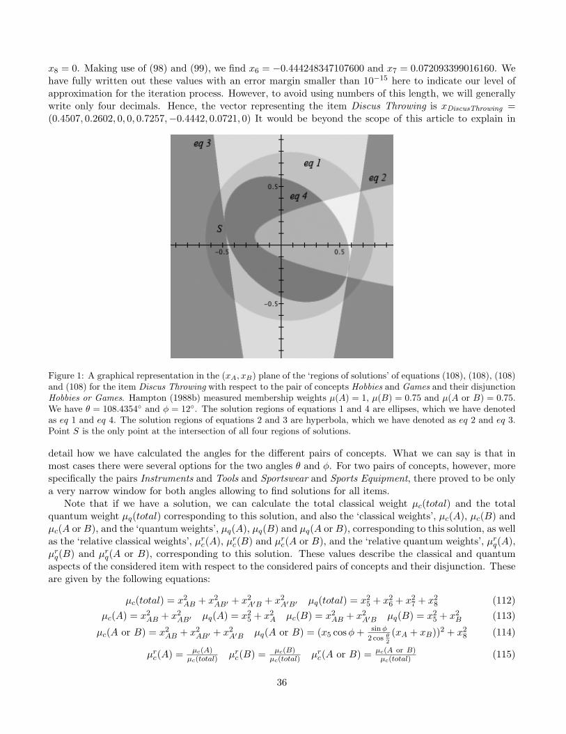
x8 = 0. Making use of (98) and (99), we find x6 = −0.444248347107600 and x7 = 0.072093399016160. Wehave fully written out these values with an error margin smaller than 10−15 here to indicate our level ofapproximation for the iteration process. However, to avoid using numbers of this length, we will generallywrite only four decimals. Hence, the vector representing the item Discus Throwing is xDiscusThrowing =(0.4507, 0.2602, 0, 0, 0.7257,−0.4442, 0.0721, 0) It would be beyond the scope of this article to explain in

Figure 1: A graphical representation in the (xA, xB) plane of the ‘regions of solutions’ of equations (108), (108), (108)and (108) for the item Discus Throwing with respect to the pair of concepts Hobbies and Games and their disjunctionHobbies or Games. Hampton (1988b) measured membership weights µ(A) = 1, µ(B) = 0.75 and µ(A or B) = 0.75.We have θ = 108.4354 and φ = 12. The solution regions of equations 1 and 4 are ellipses, which we have denotedas eq 1 and eq 4. The solution regions of equations 2 and 3 are hyperbola, which we have denoted as eq 2 and eq 3.Point S is the only point at the intersection of all four regions of solutions.

detail how we have calculated the angles for the different pairs of concepts. What we can say is that inmost cases there were several options for the two angles θ and φ. For two pairs of concepts, however, morespecifically the pairs Instruments and Tools and Sportswear and Sports Equipment, there proved to be onlya very narrow window for both angles allowing to find solutions for all items.

Note that if we have a solution, we can calculate the total classical weight µc(total) and the totalquantum weight µq(total) corresponding to this solution, and also the ‘classical weights’, µc(A), µc(B) andµc(A or B), and the ‘quantum weights’, µq(A), µq(B) and µq(A or B), corresponding to this solution, as wellas the ‘relative classical weights’, µrc(A), µrc(B) and µrc(A or B), and the ‘relative quantum weights’, µrq(A),µrq(B) and µrq(A or B), corresponding to this solution. These values describe the classical and quantumaspects of the considered item with respect to the considered pairs of concepts and their disjunction. Theseare given by the following equations:

µc(total) = x2AB + x2

AB′ + x2A′B + x2

A′B′ µq(total) = x25 + x2

6 + x27 + x2

8 (112)µc(A) = x2

AB + x2AB′ µq(A) = x2

5 + x2A µc(B) = x2

AB + x2A′B µq(B) = x2

5 + x2B (113)

µc(A or B) = x2AB + x2

AB′ + x2A′B µq(A or B) = (x5 cosφ+ sinφ

2 cos θ2

(xA + xB))2 + x28 (114)

µrc(A) = µc(A)µc(total)

µrc(B) = µc(B)µc(total)

µrc(A or B) = µc(A or B)µc(total)

(115)

36

µrq(A) = µq(A)µq(total)

µrq(B) = µq(B)µq(total)

µrq(A or B) = µq(A or B)µq(total)

(116)

To further clarify the meaning of these new quantities, let us calculate them for the case of the solutionwe found for the item Discus Throwing with respect to the pair of concepts Hobbies and Games andtheir disjunction Hobbies or Games. We find µc(total) = 0.2708, µq(total) = 0.7292, µc(A) = 0.2708,µq(A) = 0.7292, µc(B) = 0.2031, µq(B) = 0.5469, µc(A or B) = 0.2708, µq(A or B) = 0.4292, µrc(A) = 1,µrc(B) = 0.75, µrc(A or B) = 1, µrq(A) = 1, µrq(B) = 0.75 and µrq(A or B) = 0.5886.

A closer examination of the ‘relative classical and quantum weights’ is the most revealing for it showsus that the relative weights of the item Discus Throwing equal the originally measured weights for bothconcepts A and B. The relative classical weight of the item with respect to the disjunction equals 1,which is the maximum of the weights with respect to both concepts. This means that the relative classicalweight satisfies the maximum rule of fuzzy set theory. The relative quantum weight with respect to thedisjunction is 0.5886, which is smaller than the original weight of 0.7 with respect to the disjunction. Thismeans that the relative quantum weight ‘confirms’ the underextension measured in the experiment. Infact, the measured underextension is a result of the quantum aspects of the item, and the underextensionfor the relative quantum weights is stronger than the underextension measured. Mixed with the ‘maximumrule satisfying relative classical weight’ it results in the underextension measured in the experiment.

A more correct interpretation would be to acknowledge the effect of ‘quantum superposition’. Theclassical aspect, expressed by the relative classical weights, behaves in line with the maximum rule of fuzzyset for the disjunction, while the quantum aspect gives rise to underextension.

Before we proceed, we will introduce an extra condition, which we will call the ‘modularity condition’.This condition is that the classical weights, i.e. the weights that would result if only the classical aspectsof the item were involved, must be proportional to the measured weights for both concepts A and B. Thereason for this condition is that on measuring µ(A) and µ(B), there is no combination of concepts yet. Thisimplies that the classical weight involving a combination should be proportional to the weights that donot involve a combination. In this way the classical weights will be the same, subject to a proportionalityfactor, if the concepts under consideration are combined with other concepts. The modularity conditioncan be expressed as follows:

µ(A) · µc(B) = µ(B) · µc(A) (117)

Note that the condition makes that, for µ(A) 6= 0 and µ(B) 6= 0, we have

µrc(A)µ(A)

=µc(A)

µc(total) · µ(A)=

µc(B)µc(total) · µ(B)

=µrc(B)µ(B)

(118)

which means that the ‘relative classical weights’ are proportional to the measured weights.For the item Discus Throwing, this factor of proportionality is equal to 1, and as a consequence the

relative classical weight of Discus Throwing for both concepts is equal to the measured weight. This is trueof many items, as we can see in Tables 3 and 4, where we have calculated the relative classical and relativequantum weights for all items with respect to all pairs of concepts in Hampton(1988a,b). For some itemsthe modularity factor is different from 1. Table 3 presents the values of the relative classical and quantumweights with respect to all items and pairs of concepts and their disjunctions as referred to in Hampton(1988b), and also the components of the vectors representing these items.

3.3 Working out the Conjunction Data

To model the conjunction data, we can directly use the modeling of the disjunction data worked out inthe previous sections. Indeed, suppose that we consider a pair of concepts A and B and their conjunction‘A and B’, and an item X, with µ(A), µ(B), µ(A and B) being the membership weights of item X with

37

respect to A, B and ‘A and B’. If we take equations (59), (60), (61) and (62), which determine the modelfor the disjunction and the conjunction, we can see that if we consider two hypothetical concepts A′, B′ andtheir disjunction ‘A′ or B′’ such that µ(A′) = 1−µ(A), µ(B′) = 1−µ(B) and µ(A′ or B′) = 1−µ(A and B)are the membership weights of an item X with respect to A′, B′ and their disjunction ‘A′ or B′’, the samevector x that models the item X for the concepts A′, B′ and ‘A′ or B′’, also models this item X for theconcepts A, B and ‘A and B’.

Here is a concrete example to clarify what we mean. Let us consider the item TV with respect tothe pair of concepts Furniture and Household Appliances and their conjunction ‘Furniture and HouseholdAppliances’. We have µ(A) = 0.7, µ(B) = 0.9 and µ(A and B) = 0.925. Hence we introduce A′, withµ(A′) = 1−µ(A) = 0.3, B′, with µ(B′) = 1−µ(B) = 0.1, and ‘A′ or B′’ with µ(A′or B′) = 1−µ(A and B) =0.075. Suppose we construct the vector x, as we have done in previous sections, modeling item X withrespect to A′, B′ and ‘A′ or B′’. Replacing A with A′ and B with B′ in the equations (59), (60) and (62),we obtain

µ(A′) = x2A′B′ + x2

A′B + x28 + x2

A′ (119)µ(B′) = x2

A′B′ + x2AB′ + x2

8 + x2B′ (120)

µ(A′ or B′) = x2A′B′ + x2

A′B + x2AB′ + c2

7 + c28 (121)

1 = x2A′B′ + x2

A′B + x2AB′ + x2

AB + x28 + x2

7 + x26 + x2

5 (122)

If we now apply (69), it follows from this that

µ(A) = 1− µ(A′) = x2AB + x2

AB′ + x26 + x2

7 − x2A′ = x2

AB + x2AB′ + x2

A (123)

In an analogous way, again making use of (69), it follows that

µ(B) = x2AB + x2

A′B + x2B (124)

and, making use of (70), we also get

µ(A and B) = 1− µ(A′ or B′) = x2AB + x2

8 + x27 + x2

6 + x25 − c2

7 − c28 = x2

AB + c25 + c2

6 (125)

If we compare equations (59), (60) and (61) with equations (123), (124) and (125), we can see that x modelsthe conjunction data µ(A), µ(B) and µ(A and B) of item X. In Table 4 we have calculated for each itemX and for each pair of concepts A, B and their conjunction A and B the vector xX - element of R8 - thatrepresents this item X. We have also calculated the ‘relative classical and quantum weights’ for each itemX with respect to the different pairs of concepts and their conjunction measured in Hampton (1988a).Analogous to our discussion of the disjunction, we introduce the following equations for the conjunction:

µc(A and B) = x2AB µq(A and B) = c2

5 + c26 (126)

µrc(A and B) = µc(A and B)µc(total)

µrq(A and B) = µq(A and B)µq(total)

(127)

To illustrate this, let us consider the item Library with respect to the pair of concepts Building and Dwellingand their conjunction Building and Dwelling. Hampton (1988a) measured µ(A) = 0.95, µ(B) = 0.175 andµ(A and B) = 0.3077, which is a case of ‘overextension’. Table 4 shows that vector x representing thisitem is given by xLibrary = (0.3809, 0.8015, 0, 0.2036, 0, 0.3927, 0.0919, 0.0923), and for the relative classicaland relative quantum weights we find µrc(A) = 0.95, µrc(B) = 0.175, µrc(A and B) = 0.175, µrq(A) = 0.95,µrq(B) = 0.175 and µrq(A and B) = 0.9503. The relative classical weights satisfy the minimum rule offuzzy set theory. On the other hand, the relative quantum weights involve a far greater overextension thanthat of the measured values of the membership weights in Hampton (1988a). The reason for this is that

38

these values are determined by a combination of classical and quantum aspects of the item Library. Theweights of the classical aspects that satisfy the minimum rule are responsible for keeping the overextensioncaused by the quantum aspects restricted to the moderate overextension apparent in the weights found inHampton (1988a). In the next section we will elaborate on the hypothesis that we introduced in subsection1.6 about the ‘superposed layers of the human thought’.

3.4 Classical Logical and Quantum Conceptual Thought

In section 1.6 we introduced the idea of the two ‘superposed layers of human thought’. In this section wewill give several examples to illustrate these layers, taking advantage of the explicit nature of the workedout superposition and the introduction of the corresponding relative classical and relative quantum weights.

We consider the pair of concepts Spices and Herbs and their disjunction Spices or Herbs. In Table 3we can see that different types of items have been tested by Hampton (1988b) in relation with this pairof concepts. Let us first consider one of the k-type non-classical items, for example MSG. Total classicalweight is 0.6950 and total quantum weight is 0.3050. Hence the item’s behavior is ‘more classical thanquantum’, or ‘classical logical thought’ is more dominant than ‘quantum conceptual thought’. The relativeclassical weights are µrc(A) = 0.15, µrc(B) = 0.1 and µrc(A or B) = 0.25, compared to the measured weightsof Hampton (1988b), which are µ(A) = 0.15, µ(B) = 0.1, µ(A or B) = 0.425. We can see that the weightswith respect to the individual concepts A and B are equal. However, for the weight with respect to thedisjunction, we see that the relative classical weight is less. This must be so, because MSG is a k-typenon-classical item, which means that µ(A) + µ(B) < µ(A or B). Note that the relative classical weightis exactly equal to µ(A) + µ(B), which means that the ‘classical part’ of the item has done the best itcan in coping with the k-type non-classicality, indeed µrc(A or B) = 0.25 = µrc(A) + µrc(B) is as greatas it can in order to remain classical. The relative quantum weights are µrq(A) = 0.15, µrq(B) = 0.1 andµrq(A or B) = 0.8239. Hence most of all µrq(A or B) is very great. This means that the subjects considereditem MSG to be very much characteristic of Spices or Herbs. In other words, they considered MSG to beone of those items that typically make one doubt about whether they are Spices or whether they are Herbs,while at the same time they found MSG to be not very characteristic of Spices alone, or Herbs alone. Thisis reflected by µ(A) = µrc(A) = µrq(A) = 0.15 and µ(A) = µ2

c(A) = µrq(A) = 0.1.We find a similar pattern for the other k-type non-classical items Saccharin, Sugar, Vinegar and Lemon

Juice. For Vinegar the value found is even greater: µrq(A or B) = 0.9000. The most extreme case isthat of Sugar, which subjects qualified as ‘does not belong to Spices’ (µ(A) = 0), and ‘does not belong toHerbs’ (µ(B) = 0), but ‘does belong moderately to Spices or Herbs’ (µ(A or B) = 0.2). If we look at theelements of its quantum representation in Table 3, we can see the following. We have µ2

c(A) = µrq(A) = 0and µ2

c(B) = µrq(B) = 0, which is not a surprise. Also, we have µrc(A or B) = 0, which means that thesubjects indeed did not assign any weight to the membership of the disjunction as far as this is determinedby ‘classical logical thought’. And Table 3 shows that µrq(A or B) = 1. Consequently, as far as ‘quantumconceptual thought’ is concerned, subjects decided that the membership weight of the item Sugar withrespect to the new concept Spices or Herbs equals 1. To make this more concrete, we can imagine thefollowing situation. Asked whether the item Sugar is a member of Spices or Herbs, a subject may bereasoning as follows: ‘It is clear that sugar is not a spice and nor is it a herb (which means that followingthe rules of classical logic it is not a ‘spice or herb’), but then again, sugar is a substance that one mayreadily doubt about whether it is a spice or whether it is a herb. Hence, in this sense, it is a member of‘Spices or Herbs’. As said, such thought processes do not happen serially, but in parallel, or rather, ‘insuperposition’.

Let us now turn to the ∆-type non-classical items, for example the item Salt. Subjects found it tobe much of a member of Spices (µ(A) = 0.75), but not very much a member of Herbs (µ(B) = 0.1),while the membership weight with respect to the disjunction is considerable (µ(A or B) = 0.6). ‘Classical

39

logical thought’ gives rise to values for the relative classical weights that are the following µrc(A) = 0.75,µrc(B) = 0.1, µrc(A or B) = 0.75. These values satisfy the maximum rule of fuzzy set theory, and henceare the ones one would intuitively expect for the disjunction. For the quantum relative weights we findµrq(A) = 0.75, µrq(B) = 0.1, µrq(A or B) = 0.2955. The underextension here is very significant, muchgreater than for the measured values. It means that the subjects consider Salt an item that raises hardlyany doubts as to whether it is a member of Spices or a member of Herbs, even though it is not a verystrong member of either of the two.

A similar pattern appears for the other ∆-type non-classical items with respect to this pair of concepts,Curry, Oregano, Chili Pepper, Mustard, Turmeric, Vanilla, Chires and Root Ginger. Note that many ofthese ∆-type non-classical items have a great total quantum weight, for example Mustard has µq(total) =0.6448. This means the ‘new concept’ has a great impact, also for these ∆-type non-classical items, andeven more for these than for the previously considered k-type non-classical items. But the presence ofthe ‘new concept’ can mainly be explained by the fact that the subjects do not regard these items ascharacteristic of the new concept ‘A or B’. So whereas for a k-type non-classical item, subjects will arguemore or less by saying ‘that this is an item that indeed raises doubts about whether it is a member ofSpices or a member of Herbs, for ∆-type non-classical items they will also – and very much so – take intoaccount the new concept ‘A or B’, and decide, unlike in the case of the k-type non-classical items, thatthese ∆-type non-classical items are ‘not’ characteristic of ‘A or B’ and hence ‘not’ the type of items thatraise doubts about whether they are members of A or members of B.

What about the classical items? Well, our model shows that they are not really classical. We couldhave decided to model each of the classical items purely within the classical part, i.e. the subspacegenerated by the vectors eAB, eAB′ , eA′B, eA′B′ of R8. The membership weights for classical items satisfythe inequalities characterizing classical data, so that this modeling would have been possible, as madeexplicitly clear in subsection 2.1. However, in view of the results yielded by our quantum model, it ismuch more plausible to assume that a classical item is classical only in appearance and that in realityit is a superposition of a classical item with a greater value for the disjunction than the value measuredand superposed with a ∆-type non-classical item with underextension for the disjunction. This is how wehave modeled the classical items, taking for the value of the ‘relative classical disjunction’ the medium ofthe measured value and the maximum value. Here is an example. Let us consider the item Poppyseedswith respect to the pair of concepts Spices and Herbs and their disjunction Spices or Herbs. The measuredvalues of the membership weights are µ(A) = 0.4, µ(B) = 0.4 and µ(A or B) = 0.4. The maximum value ofthe disjunction is the sum of µ(A) and µ(B), hence 0.8. Hence we have chosen to take the relative classicalweight of the disjunction equal to the medium of the maximum value 0.8 and the measured value 0.4, i.e.µrc(A or B) = 0.6. As a consequence we find µrc(A) = 0.4, µrc(B) = 0.4, µrc(A or B) = 0.6, µrq(A) = 0.4,µrq(B) = 0.4, µrq(A or B) = 0.1270. This gives a very small value for the membership weight with respectto the new concept ‘Spices or Herbs’. Subjects find Poppyseeds not at all characteristic of items that raisedoubts as to whether they are Spices or Herbs.

We have so far compared ‘classical logical thought’ and ‘quantum conceptual thought’ only for thesituation of disjunction. We will therefore now discuss an example of conjunction. We will first consider a∆-type non-classical item, for example the item Dogsled with respect to the pair of concepts Machine andVehicle and their conjunction Machine and Vehicle. The measured membership weights are µ(A) = 0.1795,µ(B) = 0.925 and µ(A and B) = 0.275. This points to a moderate overextension for the conjunction. Forthe relative classical membership weights, we find µ(A)rc = 0.1795, µ(B)rc = 0.925 and µ(A and B)rc =0.1795. This means that the minimum rule of fuzzy set theory is satisfied for the conjunction weight. For therelative quantum membership weights, we find µ(A)rq = 0.1795, µ(B)rq = 0.925 and µ(A and B)rq = 0.9829.With respect to the new concept Machine and Vehicle, and with the subjects now reflecting in terms of‘quantum conceptual thought’, Dogsled is found to be only very weakly a member of Machine (0.1795) and

40

very strongly a member of Vehicle (0.925). However, Dogsled is even more strongly a member of the newconcept ‘Machine and Vehicle’ (0.9829).

A similar pattern is found for the other ∆ type items, Bicycle, Roadroller, Elevator, Course Liner,Skateboard, Bulldozer, Lawn Mover and Ski Lift. We already said that the proportionality factor relatedto the modularity condition is not always 1, let us therefore consider a relevant example. For the itemCourse Liner we have µ(A) = 0.875, µ(B) = 0.875, µ(A and B) = 0.95, µ(A)rc = 0.9424, µ(B)rc = 0.9424,µ(A and B)rc = 0.9424, µ(A)rq = 0.4306, µ(B)rq = 0.4306 and µ(A and B)rq = 1. This means that subjectsfind Course Liner to be as much a Machine as a Vehicle, but the relative classical weights are much greater(0.9424) than the relative quantum weights (0.4306); together they middle out to the measured weights(0.875). The relative quantum weight of a member of the new concept Machine and Vehicle is 1.

4 Fundamentals of Concept Formation and Combination

The above might suggest that the process of thought we have discussed is very specific. In this sectionwe will show that it is quite the contrary, it is fundamental and directly related to the process of conceptformation.

4.1 General Concept Formation

Often a concept can be presented as the disjunction – the ‘or’ – of a set of other concepts. Let us considerthe following example. Animal can be Dog or Cat or Horse or Rabbit or . . . followed by a long list of allthe usually known animals. Barking is characteristic of Dog, so that it is fair to state that its weight withrespect to Dog would be close to 1. With respect to Animal, however, Barking is not very characteristic,so that its weight would be rather small. This indicates the effect of underextension, exactly what appearsin the Hampton (1988b) experiments with respect to the disjunction. In other words, if disjunction means‘the formation of a new concept’, then underextension is a natural effect, and also a fundamental effect.

It is also true, however, that a concept can often be presented as a conjunction – the ‘and’ – of a set ofother concepts. For example, Dog is Has four legs and Likes to Bark and Has fur and Likes to Swim and . . .followed by a long list of characteristics of a Dog. Humans Friend is characteristic of Dog, hence we couldattribute it a weight close to 1 with respect to Dog. However, Humans Friend is not very characteristicof Has Four Legs or Likes to Swim etc . . ., so that weights for these concepts would be rather small. Thisshows that if the conjunction is used to form a new concept, overextension is a natural effect, and also afundamental effect.

These examples illustrate that the effects we have been modeling in our quantum modeling schemeare natural effects related to the capacity of the human mind to form new concepts. Moreover, we canput forward an interesting line of reasoning with regard to Fodor’s Puzzle of Concept Acquisition (Fodor1975; Margolis and Laurence, 2002). As we demonstrated in the foregoing, in our theory, conjunctionand disjunction comprise two aspects which we referred to as ‘two-particle way’ and ‘one-particle way’.Usually, certainly if things are considered from a logical perspective, only the ‘two-particle way’ is identifiedas existing, and hence conjunction and disjunction appear as just ‘logical combinations that do not generatenew conceptual knowledge’ – one of Fodor’s arguments. In our quantum modeling scheme, ‘superposition’introduces a new emergent state, coming about each time concepts combine. Consequently, ‘new conceptformation’ is considered to be as important an event as the classical logical combination of concepts, andit can be readily modeled using the mathematical formalism of quantum mechanics.

41

4.2 The Modeling of Large Collections of Combinations of Concepts

In this subsection we will show how our quantum modeling scheme gives rise to a mathematical formalismfor the description of large collections of combinations of concepts. The structure of Fock space again playsa fundamental role. We will not repeat here the details of this construction, which can be found in Aerts(2007b), but only outline its basic elements and suggest the potential of this approach.

Let us consider the situation of a combination of n concepts and in parallel consider a concrete example,namely the sentence ‘The cat eats the food while the child plays in the garden’, which is a combinationof 12 concepts. For a combination of n concepts, the quantum superposition state that corresponds to‘considering the combination as one new concept’ is the state 1√

n

∑ni=1 |An〉 where |Ai〉 is the state of

concept number i, and 〈Ai|Ai〉 = 1 while 〈Ai|Aj〉 = 0 for i 6= j, all this defined in a Hilbert space H. Hencethe state which describes the example sentence as ‘one new concept’ is given by 1√

12

∑12i=1 |A12〉. Note

that some concepts of such a large combination carry much more meaning than others with respect to agiven context. This difference is accounted for by introducing a more general superposition state, i.e. aweighted linear combination instead of a sum, as demonstrated in Aerts (2007b), but we will not considerthis situation here. The state where the n concepts are considered individually, and where only their logicalcombinations are taken into account, is the state |A1〉⊗ . . .⊗|Ai〉⊗ . . .⊗|An〉 element of the n-times tensorproduct H⊗ . . .⊗H. Hence, for the example sentence, this is the state |A1〉⊗ . . .⊗|Ai〉⊗ . . .⊗|A12〉. Theseare the two end-elements of the direct sum of Hilbert spaces that Fock space is, the first containing thedescription of the whole combination as one new concept, and the second containing the description of thecombination as a classical combination of concepts. In between there are parts of the complete state thatcontain the effects due to the fact that ‘also parts of the combination can be considered as whole and newconcepts’. In the example sentence, ‘The cat eats the food’ and ‘While the child plays in the garden’ aregood examples of parts that will be assigned considerable weight for being considered ‘new concepts of theirown’. How can Fock space provide a description for all these possibilities? Let us demonstrate this usingthe same example. The first part of the sentence consists of a combination of five concepts, so that thestate 1√

5

∑5i=1 |A5〉 is the state that describes this part of the sentence as a whole new concept. The second

part of the sentence consists of the seven remaining concepts. Hence the state 1√7

∑6i=1 |A12〉 describes this

part of sentence as a whole new concept. We now have a situation with ‘two concepts’, i.e. one for each ofboth parts of the sentence. This situation is described by 1√

5

∑5i=1 |A5〉⊗ 1√

7

∑6i=1 |A12〉 element of the two

times tensor product H⊗H. This is how the Fock space model of our quantum modeling scheme realizeseach possibility of considering certain subsets of the combination of n concepts as individual concepts.

Fock space can become very extensive as in quantum field theory when it describes the micro-world, sothat it is important to consider possibilities of approximation. The guiding idea of such approximate mod-eling is linked to what we have understood so far with respect to our general modeling scheme. Consideringthe example sentence, we can ask the question ‘how many instantiations are there primarily involved inthe scenery of this sentence?’. Clearly, the concepts Cat, Food, Child and Garden give rise to instantiationswithin possible situations described by the sentence. This means that a ‘four-entity way’, with the statedescribed by a vector in a 4-times tensor product H ⊗ H ⊗ H ⊗ H, will be a possible first-order approx-imate model for this sentence. If the scenery described by the sentence considers also the concepts Eatand Play as giving rise to instantiations, we get an extra element for an eventually better approximation.By adding Eat and Play to the set of concepts that determine the basic dimension of the tensor productcomponent, we take into account ‘ways of eating’, which gives rise to states for the concept Eat, and ‘waysof playing’, which gives rise to states for the concept Play. This would result in a 6-times tensor productspace description. The direct sum of both is an element of Fock space.

In principle, our quantum modeling scheme, with the construction of the state in Fock space as outlinedabove, extends to very large parts of combinations of concepts, pieces of text, documents, collections

42

of documents, books etc . . . . We will have to investigate the validity of this modeling by performingquantitative experiments and measuring weights related to typicalities of items and applicability of features,as we did in Aerts and Gabora (2005a,b) to prove the presence of contextual influence. Basing ourselveson the concrete modeling of the data found in Hampton (1988a,b), we are confident about the outcome.

Table 3: For each item X and for each pair of concepts A, B and their disjunc-tion A or B we calculate the vector x, element of R8, that represents this itemX. We also calculate the ‘relative classical’ and ‘relative quantum weights’ asdefined in (115) and (116), and the total quantum weight µq defined in (112).The total classical weight equals 1 minus the total quantum weight. Undereach item we specify its type, ∆ means ∆-type non-classical, k means k-typenon-classical, and c means classical.

Item µ(A) µ(B) µ(A or B)µrc(A) µrc(B) µrc(A or B)µrq(A) µrq(B) µrq(A or B)µqtype xAB xAB′ xA′B xA′B′ x5 x6 x7 x8 xA xB

A=Home Furnishing, B=Furniture, θ = 131.1440, φ = 0

Mantelpiece 0.8 0.4 0.75 0.8 0.4 0.8 0.8 0.4 0.4414 0.1394∆ 0.5867 0.5867 0 0.4149 0.1918 -0.2756 0.0437 0.1574 -0.1378 0.2734Window Seat 0.9 0.9 0.8 0.9 0.9 0.9 0.9 0.9 0.7236 0.5667∆ 0.6244 0 0 0.2081 0.6166 -0.2799 0.2799 0.1729 -0.3604 0.3604Painting 0.9 0.5 0.85 0.9 0.5 0.9 0.9 0.5 0.4680 0.1157∆ 0.6649 0.5947 0 0.2974 0.2216 -0.2480 0.0070 0.0712 -0.2347 0.0937Light Fixture 0.8 0.4 0.775 0.8 0.4 0.8 0.8 0.4 0.4512 0.0717∆ 0.6094 0.6094 0 0.4309 0.1417 -0.1967 0.0251 0.1107 -0.1930 0.0926Kitchen Count 0.8 0.55 0.625 0.8 0.55 0.8 0.8 0.55 0.5077 0.5987∆ 0.4698 0.3167 0 0.2833 0.4303 -0.4967 0.2191 0.3447 -0.5420 0.3796Bath Tub 0.5 0.7 0.75 0.5 0.7 0.875 0.5 0.7 0.7344 0.8891c 0.1898 0.1393 0.2039 0.1177 0.6445 0 0.4859 0.4874 -0.1708 0.4550Deck Chair 0.1 0.3 0.35 0.1 0.3 0.375 0.1 0.3 0.0208 0.0706c 0.1524 0.2640 0.5056 0.7622 0.0380 0.1587 0.2096 0.0047 0.0749 0.1405Shelves 1 0.4 1 1 0.4 1 0 0 0 0c 0.6325 0.7746 0 0 0 0 0 0 0 0Rug 0.9 0.6 0.95 0.9 0.6 0.975 0.9 0.6 0.0601 0.0273c 0.7146 0.6039 0.2701 0.1559 0.0009 -0.1352 0.0860 0.0405 -0.1568 0.1280Bed 1 1 1 1 1 1 0 0 0 0c 1 0 0 0 0 0 0 0 0 0Wall-Hangings 0.9 0.4 0.95 0.9 0.4 0.975 0.9 0.4 0.1 0.0286c 0.5619 0.7474 0.2699 0.1558 0.0019 -0.1495 0.0581 0.0534 -0.1603 0.1069Space Rack 0.7 0.5 0.65 0.7 0.5 0.7 0.7 0.5 0.6096 0.5530∆ 0.4728 0.2990 0 0.3662 0.4145 -0.4259 0.1858 0.4066 -0.4640 0.3236Ashtray 0.7 0.3 0.25 0.4546 0.1948 0.4546 1 0.4286 0 0.45∆ 0.3273 0.3780 0 0.5477 0 -0.6291 0.2330 0 -0.6708 0.4392Bar 0.35 0.6 0.55 0.35 0.6 0.6 0.35 0.6 0.5154 0.5909∆ 0.3784 0 0.3198 0.4045 0.2624 -0.2124 0.4912 0.4855 -0.3714 0.5345Lamp 1 0.7 0.9 1 0.7 1 1 0.7 0.4710 0.1890∆ 0.7534 0.4932 0 0 0.2984 -0.2961 0.1111 0 -0.3162 0.2081Wall Mirror 1 0.6 0.95 1 0.6 1 1 0.6 0.2946 0.0709∆ 0.7466 0.6096 0 0 0.1445 -0.2093 0.0786 0 -0.2236 0.1471Door Bell 0.5 0.1 0.55 0.5 0.1 0.575 0.4747 0.0949 0.4883 0.4337c 0.1213 0.5286 0.21 0.5 0.0139 -0.4694 0.0401 0.46 -0.4535 0.2024Hammock 0.2 0.5 0.35 0.2 0.5 0.5 0.2 0.5 0.1752 0.4618∆ 0.3281 0 0.4018 0.5187 0.2844 0.3138 0.5314 0.0001 0.1070 0.3873Desk 1 1 1 1 1 1 0 0 0 0c 1 0 0 0 0 0 0 0 0 0Refrigerator 0.9 0.7 0.575 0.9 0.7 0.9 0.9 0.7 0.4324 0.6950∆ 0.4621 0.2470 0 0.1747 0.4940 -0.5381 0.3240 0.2376 -0.6176 0.4924Park Bench 0 0.3 0.05 0 0.0531 0.0531 0 0.5404 0.0470 0.5066∆ 0 0 0.1619 0.6835 0 -0.2442 -0.6505 0.1543 0 0.5233Waste Paper Basket 1 0.5 0.6 1 0.5 1 1 0.5 0.1183 0.4537∆ 0.5226 0.5226 0 0 0.2317 -0.5921 0.2222 0 -0.6325 0.4161Sculpture 0.8 0.4 0.8 0.8 0.4 0.9 0.8 0.4 0.3931 0.1973c 0.4907 0.6335 0.2833 0.2833 0.2785 0.3351 0.0864 0 -0.2833 0.0368Sink Unit 0.9 0.6 0.6 0.9 0.6 0.9 0.9 0.6 0.4212 0.6265∆ 0.4734 0.3347 0 0.1933 0.4494 -0.5533 0.2378 0.2487 -0.6015 0.4170

43

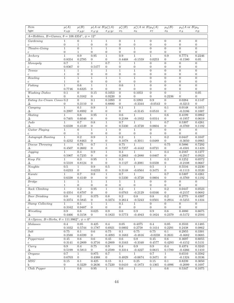
Item µ(A) µ(B) µ(A or B)µrc(A) µrc(B) µrc(A or B)µq(A) µq(B) µq(A or B)µqtype xAB xAB′ xA′B xA′B′ x5 x6 x7 x8 xA xB

A=Hobbies, B=Games, θ = 108.4354, φ = 12

Gardening 1 0 1 1 0 1 0 0 0 0c 0 1 0 0 0 0 0 0 0 0Theatre-Going 1 0 1 1 0 1 0 0 0 0c 0 1 0 0 0 0 0 0 0 0Archery 1 0.9 0.95 1 0.9 1 1 0.9 0.7774 0.2246∆ 0.8354 0.2785 0 0 0.4468 -0.1559 0.0253 0 -0.1580 0.05Monopoly 0.7 1 1 0.7 1 1 0 0 0 0c 0.8367 0 0.5477 0 0 0 0 0 0 0Tennis 1 1 1 1 1 1 0 0 0 0c 1 0 0 0 0 0 0 0 0 0Bowling 1 1 1 1 1 1 0 0 0 0c 1 0 0 0 0 0 0 0 0 0Fishing 1 0.6 1 1 0.6 1 0 0 0 0c 0.7746 0.6325 0 0 0 0 0 0 0 0Washing Dishes 0.1 0 0.15 0.1053 0 0.1053 0 0 1 0.05k 0 0.3162 0 0.9220 0 0 0 0.2236 0 0Eating Ice-Cream Cones 0.2 0 0.1 0.1093 0 0.1093 0.9 0 0.0284 0.1147∆ 0 0.3110 0 0.8880 0 -0.3344 -0.0543 0 -0.3213 0Camping 1 0.1 0.9 1 0.1 1 1 0.1 0.0148 0.1015∆ 0.2997 0.8992 0 0 0 -0.3145 0.0510 0 -0.3186 0.1007Skating 1 0.6 0.95 1 0.6 1 1 0.6 0.4199 0.0862∆ 0.7405 0.6046 0 0 0.2188 -0.1932 0.0314 0 -0.1957 0.0619Judo 1 0.7 0.8 1 0.7 1 1 0.7 0.5307 0.4261∆ 0.6338 0.4149 0 0 0.5330 -0.3720 0.0604 0 -0.3769 0.1192Guitar Playing 1 0 1 1 0 1 0 0 0 0c 0 1 0 0 0 0 0 0 0 0Autograph Hunting 1 0.2 0.9 1 0.2 1 1 0.2 0.0447 0.1047∆ 0.4232 0.8463 0 0 0.1078 -0.3011 0.0489 0 -0.3050 0.0965Discus Throwing 1 0.75 0.7 1 0.75 1 1 0.75 0.5886 0.7292∆ 0.4507 0.2602 0 0 0.7257 -0.4442 0.0721 0 -0.4501 0.1423Jogging 1 0.4 0.9 1 0.4 1 1 0.4 0.2167 0.1277∆ 0.5907 0.7235 0 0 0.2063 -0.2880 0.0467 0 -0.2917 0.0923Keep Fit 1 0.3 0.95 1 0.3 1 1 0.3 0.1252 0.0572∆ 0.5318 0.8124 0 0 0.1127 -0.2081 0.0338 0 -0.2108 0.0667Noughts 0.5 1 0.9 0.5 1 1 0.5 1 0.5516 0.2230∆ 0.6233 0 0.6233 0 0.3148 -0.0564 0.3475 0 -0.1113 0.3520Karate 1 0.7 0.8 1 0.7 1 1 0.7 0.5307 0.4261∆ 0.6338 0.4149 0 0 0.5330 -0.3720 0.0604 0 -0.3769 0.1192Bridge 1 1 1 1 1 1 0 0 0 0c 1 0 0 0 0 0 0 0 0 0Rock Climbing 1 0.2 0.95 1 0.2 1 1 0.2 0.0447 0.0523∆ 0.4354 0.8707 0 0 0.0763 -0.2129 0.0346 0 -0.2157 0.0682Beer Drinking 0.8 0.2 0.575 0.8 0.2 0.8 0.8 0.2 0.2775 0.4307∆ 0.3374 0.5845 0 0.3374 0.2614 -0.5243 0.0501 0.2914 -0.5255 0.1334Stamp Collecting 1 0.1 1 1 0.1 1 0 0 0 0c 0.3162 0.9487 0 0 0 0 0 0 0 0Wrestling 0.9 0.6 0.625 0.9 0.6 0.9 0.9 0.6 0.4880 0.6675∆ 0.4466 0.3158 0 0.1823 0.5773 -0.4943 0.1824 0.2379 -0.5172 0.2593

A=Spices, B=Herbs, θ = 111.9962, φ = 0

Molasses 0.4 0.05 0.425 0.4 0.05 0.4375 0.4 0.05 0.3533 0.1485c 0.1032 0.5744 0.1787 0.6921 0.0002 0.2758 0.1414 0.2291 0.2438 0.0862Salt 0.75 0.1 0.6 0.75 0.1 0.75 0.75 0.1 0.2955 0.3301∆ 0.2588 0.6599 0 0.4093 0.1683 -0.4816 -0.0238 0.2631 -0.4682 0.0685Peppermint 0.45 0.6 0.6 0.45 0.6 0.8 0.45 0.6 0.4697 0.6055c 0.3141 0.2809 0.3716 0.2809 0.3163 -0.3340 0.4577 0.4293 -0.4152 0.5131Curry 0.9 0.4 0.75 0.9 0.4 0.9 0.9 0.4 0.4374 0.3243∆ 0.5199 0.5813 0 0.2599 0.3314 -0.4227 0.0615 0.1789 -0.4266 0.1410Oregano 0.7 1 0.875 0.7 1 1 0.7 1 0.6510 0.3582∆ 0.6703 0 0.4388 0 0.4829 -0.0674 0.3471 0 -0.1324 0.3536MSG 0.15 0.1 0.425 0.15 0.1 0.25 0.15 0.1 0.8239 0.3050k 0 0.3229 0.2636 0.7220 0.0410 -0.1873 0.1365 0.4996 -0.2099 0.1697Chili Pepper 1 0.6 0.95 1 0.6 1 1 0.6 0.5347 0.1075

44

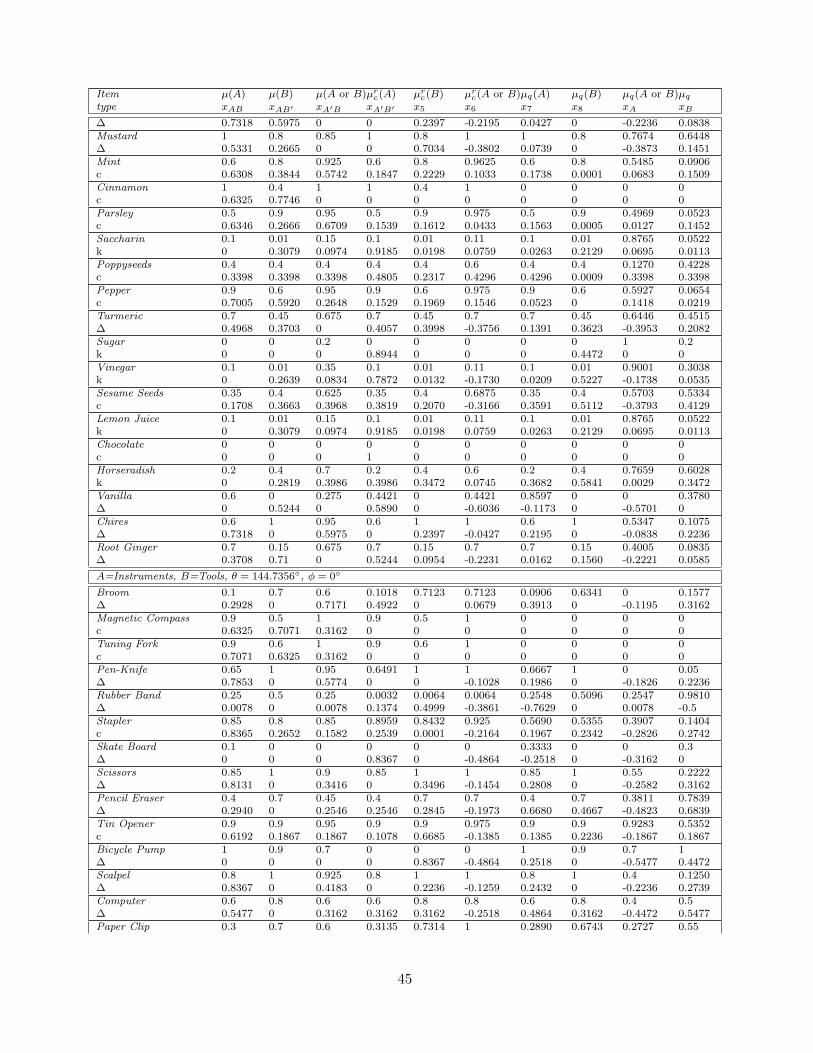
Item µ(A) µ(B) µ(A or B)µrc(A) µrc(B) µrc(A or B)µq(A) µq(B) µq(A or B)µqtype xAB xAB′ xA′B xA′B′ x5 x6 x7 x8 xA xB

∆ 0.7318 0.5975 0 0 0.2397 -0.2195 0.0427 0 -0.2236 0.0838Mustard 1 0.8 0.85 1 0.8 1 1 0.8 0.7674 0.6448∆ 0.5331 0.2665 0 0 0.7034 -0.3802 0.0739 0 -0.3873 0.1451Mint 0.6 0.8 0.925 0.6 0.8 0.9625 0.6 0.8 0.5485 0.0906c 0.6308 0.3844 0.5742 0.1847 0.2229 0.1033 0.1738 0.0001 0.0683 0.1509Cinnamon 1 0.4 1 1 0.4 1 0 0 0 0c 0.6325 0.7746 0 0 0 0 0 0 0 0Parsley 0.5 0.9 0.95 0.5 0.9 0.975 0.5 0.9 0.4969 0.0523c 0.6346 0.2666 0.6709 0.1539 0.1612 0.0433 0.1563 0.0005 0.0127 0.1452Saccharin 0.1 0.01 0.15 0.1 0.01 0.11 0.1 0.01 0.8765 0.0522k 0 0.3079 0.0974 0.9185 0.0198 0.0759 0.0263 0.2129 0.0695 0.0113Poppyseeds 0.4 0.4 0.4 0.4 0.4 0.6 0.4 0.4 0.1270 0.4228c 0.3398 0.3398 0.3398 0.4805 0.2317 0.4296 0.4296 0.0009 0.3398 0.3398Pepper 0.9 0.6 0.95 0.9 0.6 0.975 0.9 0.6 0.5927 0.0654c 0.7005 0.5920 0.2648 0.1529 0.1969 0.1546 0.0523 0 0.1418 0.0219Turmeric 0.7 0.45 0.675 0.7 0.45 0.7 0.7 0.45 0.6446 0.4515∆ 0.4968 0.3703 0 0.4057 0.3998 -0.3756 0.1391 0.3623 -0.3953 0.2082Sugar 0 0 0.2 0 0 0 0 0 1 0.2k 0 0 0 0.8944 0 0 0 0.4472 0 0Vinegar 0.1 0.01 0.35 0.1 0.01 0.11 0.1 0.01 0.9001 0.3038k 0 0.2639 0.0834 0.7872 0.0132 -0.1730 0.0209 0.5227 -0.1738 0.0535Sesame Seeds 0.35 0.4 0.625 0.35 0.4 0.6875 0.35 0.4 0.5703 0.5334c 0.1708 0.3663 0.3968 0.3819 0.2070 -0.3166 0.3591 0.5112 -0.3793 0.4129Lemon Juice 0.1 0.01 0.15 0.1 0.01 0.11 0.1 0.01 0.8765 0.0522k 0 0.3079 0.0974 0.9185 0.0198 0.0759 0.0263 0.2129 0.0695 0.0113Chocolate 0 0 0 0 0 0 0 0 0 0c 0 0 0 1 0 0 0 0 0 0Horseradish 0.2 0.4 0.7 0.2 0.4 0.6 0.2 0.4 0.7659 0.6028k 0 0.2819 0.3986 0.3986 0.3472 0.0745 0.3682 0.5841 0.0029 0.3472Vanilla 0.6 0 0.275 0.4421 0 0.4421 0.8597 0 0 0.3780∆ 0 0.5244 0 0.5890 0 -0.6036 -0.1173 0 -0.5701 0Chires 0.6 1 0.95 0.6 1 1 0.6 1 0.5347 0.1075∆ 0.7318 0 0.5975 0 0.2397 -0.0427 0.2195 0 -0.0838 0.2236Root Ginger 0.7 0.15 0.675 0.7 0.15 0.7 0.7 0.15 0.4005 0.0835∆ 0.3708 0.71 0 0.5244 0.0954 -0.2231 0.0162 0.1560 -0.2221 0.0585

A=Instruments, B=Tools, θ = 144.7356, φ = 0

Broom 0.1 0.7 0.6 0.1018 0.7123 0.7123 0.0906 0.6341 0 0.1577∆ 0.2928 0 0.7171 0.4922 0 0.0679 0.3913 0 -0.1195 0.3162Magnetic Compass 0.9 0.5 1 0.9 0.5 1 0 0 0 0c 0.6325 0.7071 0.3162 0 0 0 0 0 0 0Tuning Fork 0.9 0.6 1 0.9 0.6 1 0 0 0 0c 0.7071 0.6325 0.3162 0 0 0 0 0 0 0Pen-Knife 0.65 1 0.95 0.6491 1 1 0.6667 1 0 0.05∆ 0.7853 0 0.5774 0 0 -0.1028 0.1986 0 -0.1826 0.2236Rubber Band 0.25 0.5 0.25 0.0032 0.0064 0.0064 0.2548 0.5096 0.2547 0.9810∆ 0.0078 0 0.0078 0.1374 0.4999 -0.3861 -0.7629 0 0.0078 -0.5Stapler 0.85 0.8 0.85 0.8959 0.8432 0.925 0.5690 0.5355 0.3907 0.1404c 0.8365 0.2652 0.1582 0.2539 0.0001 -0.2164 0.1967 0.2342 -0.2826 0.2742Skate Board 0.1 0 0 0 0 0 0.3333 0 0 0.3∆ 0 0 0 0.8367 0 -0.4864 -0.2518 0 -0.3162 0Scissors 0.85 1 0.9 0.85 1 1 0.85 1 0.55 0.2222∆ 0.8131 0 0.3416 0 0.3496 -0.1454 0.2808 0 -0.2582 0.3162Pencil Eraser 0.4 0.7 0.45 0.4 0.7 0.7 0.4 0.7 0.3811 0.7839∆ 0.2940 0 0.2546 0.2546 0.2845 -0.1973 0.6680 0.4667 -0.4823 0.6839Tin Opener 0.9 0.9 0.95 0.9 0.9 0.975 0.9 0.9 0.9283 0.5352c 0.6192 0.1867 0.1867 0.1078 0.6685 -0.1385 0.1385 0.2236 -0.1867 0.1867Bicycle Pump 1 0.9 0.7 0 0 0 1 0.9 0.7 1∆ 0 0 0 0 0.8367 -0.4864 0.2518 0 -0.5477 0.4472Scalpel 0.8 1 0.925 0.8 1 1 0.8 1 0.4 0.1250∆ 0.8367 0 0.4183 0 0.2236 -0.1259 0.2432 0 -0.2236 0.2739Computer 0.6 0.8 0.6 0.6 0.8 0.8 0.6 0.8 0.4 0.5∆ 0.5477 0 0.3162 0.3162 0.3162 -0.2518 0.4864 0.3162 -0.4472 0.5477Paper Clip 0.3 0.7 0.6 0.3135 0.7314 1 0.2890 0.6743 0.2727 0.55

45

Item µ(A) µ(B) µ(A or B)µrc(A) µrc(B) µrc(A or B)µq(A) µq(B) µq(A or B)µqtype xAB xAB′ xA′B xA′B′ x5 x6 x7 x8 xA xB

∆ 0.1421 0.3476 0.5558 0 0 -0.1283 0.6193 0.3873 -0.3987 0.6090Paint Brush 0.65 0.9 0.95 0.65 0.9 0.975 0.65 0.9 0.5665 0.0612c 0.7347 0.2653 0.5524 0.1532 0.1862 0.0038 0.1628 0 -0.0715 0.1429Step Ladder 0.2 0.9 0.85 0.2183 0.9825 0.9825 0.1197 0.5384 0.2692 0.1857∆ 0.4216 0 0.7888 0.1195 0 0.0225 0.3677 0.2236 -0.1491 0.3162Door Key 0.3 0.1 0.95 0.8333 0.2778 0.8611 0 0 1 0.64k 0.3 0.4583 0.1 0.2236 0 0 0 0.8 0 0Measuring Calipers 0.9 1 0.9 0.9 1 1 0.9 1 0.7 0.3333∆ 0.7746 0 0.2582 0 0.4830 -0.1454 0.2808 0 -0.2582 0.3162Toothbrush 0.4 0.4 0.5 0.4 0.4 0.65 0.4 0.4 0.3394 0.4829c 0.2785 0.3595 0.3595 0.4254 0.4048 0.3994 0.3994 0 0.1711 0.1711Sellotape 0.1 0.2 0.325 0.1 0.2 0.3 0.1 0.2 0.6355 0.0745k 0 0.3042 0.4302 0.8049 0.0857 0.0844 0.1415 0.2 0.0099 0.0869Goggles 0.2 0.3 0.15 0.1176 0.1765 0.1765 0.6667 1 0 0.15∆ 0.3162 0 0.2236 0.8367 0 -0.1780 0.3439 0 -0.3162 0.3873Spoon 0.65 0.9 0.7 0.6610 0.9153 0.9153 0.6375 0.8827 0.4563 0.4690∆ 0.5925 0 0.3674 0.2121 0.4050 -0.1671 0.4765 0.2236 -0.3674 0.5Pliers 0.8 1 1 0.8 1 1 0 0 0 0c 0.8944 0 0.4472 0 0 0 0 0 0 0Meat Thermometer 0.75 0.8 0.9 0.75 0.8 0.95 0.75 0.8 0.8829 0.7449c 0.3912 0.1956 0.2259 0.1129 0.7468 -0.1066 -0.2755 0.3162 0.0319 -0.1956

A=Pets, B=Farmyard Animals, θ = 90, φ = 0

Goldfish 1 0 0.95 1 0 1 0 0 0 0.05∆ 0 0.9747 0 0 0 -0.2236 0 0 -0.2236 0Robin 0.1 0.1 0.1 0.1 0.1 0.1 0 0 0 0c 0.3162 0 0 0.9487 0 0 0 0 0 0Blue-Tit 0.1 0.1 0.1 0.1 0.1 0.1 0 0 0 0c 0.3162 0 0 0.9487 0 0 0 0 0 0Collie Dog 1 0.7 1 1 0.7 1 0 0 0 0c 0.8367 0.5477 0 0 0 0 0 0 0 0Camel 0.4 0 0.1 0.1429 0 0.1428 1 0 0 0.3∆ 0 0.3162 0 0.7746 0 -0.5477 0 0 -0.5477 0Squirrel 0.2 0.1 0.1 0.1176 0.0588 0.1176 0.6667 0.3333 0 0.15∆ 0.2236 0.2236 0 0.8660 0 -0.3162 0.2236 0 -0.3162 0.2236Guide Dog for the Blind 0.7 0 0.9 0.875 0 0.875 0 0 1 0.2k 0 0.8367 0 0.3162 0 0 0 0.4472 0 0Spider 0.5 0.35 0.55 0.5 0.35 0.7 0.5 0.35 0.15 0.2727c 0.3303 0.5045 0.3814 0.4671 0 0.3693 0.3090 0.2023 0.3693 0.3090Homing Pig 0.9 0.1 0.8 0.9 0.1 0.9 0.9 0.1 0.2 0.1429∆ 0.2928 0.8281 0 0.2928 0.1195 -0.3381 0 0.1195 -0.3381 0Monkey 0.5 0 0.25 0.3333 0 0.3333 1 0 0 0.25∆ 0 0.5 0 0.7071 0 -0.5 0 0 -0.5 0Circus Horse 0.4 0 0.3 0.3333 0 0.3333 1 0 0 0.1∆ 0 0.5477 0 0.7746 0 -0.3162 0 0 -0.3162 0Prize Bull 0.1 1 0.9 0.1 1 1 0.1 1 0.1 0.1111∆ 0.2981 0 0.8944 0 0.1054 0 0.3162 0 0 0.3162Rat 0.5 0.7 0.4 0.5 0.7 0.7 0.5 0.7 0.2 0.6∆ 0.4472 0 0.2828 0.3464 0.3464 -0.4243 0.5477 0 -0.4243 0.5477Badger 0 0.25 0.1 0 0.1176 0.1176 0 1 0 0.15∆ 0 0 0.3162 0.8660 0 0 0.3873 0 0 0.3873Siamese Cat 1 0.1 0.95 1 0.1 1 1 0.1 0.1 0.0556∆ 0.3073 0.9220 0 0 0.0745 -0.2236 0 0 -0.2236 0Race Horse 0.6 0.25 0.65 0.6 0.25 0.75 0.6 0.25 0.15 0.1667c 0.2887 0.6455 0.3536 0.4564 0 0.3162 0.2041 0.1581 0.3162 0.2041Fox 0.1 0.3 0.2 0.0765 0.2294 0.2294 0.2456 0.7367 0.0182 0.1392∆ 0.2566 0 0.3628 0.8145 -0.0053 0.1848 0.3202 -0.05 0.1848 0.3202Donkey 0.5 0.9 0.7 0.5 0.9 0.9 0.5 0.9 0.6 0.6667∆ 0.4082 0 0.3651 0.1826 0.5774 0 0.5164 0.2582 0 0.5164Field Mouse 0.1 0.7 0.4 0.1 0.7 0.7 0.1 0.7 0.2447 0.6589∆ 0.1847 0 0.4524 0.3199 0.1214 0.2262 0.6682 0.3828 0.2262 0.6682Ginger Tom-Cat 1 0.8 0.95 1 0.8 1 1 0.8 0.8 0.25∆ 0.7746 0.3873 0 0 0.4472 -0.2236 0 0 -0.2236 0Husky in Sledream 0.4 0 0.425 0.4103 0 0.4103 0 0 1 0.0250

46

Item µ(A) µ(B) µ(A or B)µrc(A) µrc(B) µrc(A or B)µq(A) µq(B) µq(A or B)µqtype xAB xAB′ xA′B xA′B′ x5 x6 x7 x8 xA xB

k 0 0.6325 0 0.7583 0 0 0 0.1581 0 0Cart Horse 0.4 1 0.85 0.4 1 1 0.4 1 0.4 0.25∆ 0.5477 0 0.6708 0 0.3162 0 0.3873 0 0 0.3873Chicken 0.3 1 0.95 0.3 1 1 0.3 1 0.3 0.0714∆ 0.5278 0 0.8062 0 0.1464 0 0.2236 0 0 0.2236Doberman Guard Dog 0.6 0.85 0.8 0.6 0.85 0.85 0.6 0.85 0.75 0.5∆ 0.5477 0 0.3536 0.2739 0.5477 0 0.3536 0.2739 0 0.3536

A=Sportswear, B=Sports Equipment, θ = 107, φ = 12.95

American Foot 1 1 1 1 1 1 0 0 0 0c 1 0 0 0 0 0 0 0 0 0Referee’s Whistle 0.6 0.2 0.45 0.6 0.2 0.6 0.6 0.2 0.4035 0.7635∆ 0.2175 0.3076 0 0.3076 0.2177 -0.6126 0.2366 0.5337 -0.6409 0.3245Circus Clowns 0 0 0.1 0 0 0 0 0 1 0.1k 0 0 0 0.9487 0 0 0 0.3162 0 0Backpack 0.6 0.5 0.6 0.6 0.5 0.8 0.6 0.5 0.4855 0.6359c 0.3305 0.3305 0.2699 0.2699 0.3883 -0.4336 0.3486 0.4190 -0.4804 0.4089Diving Mask 1 1 0.95 1 1 1 1 1 0.9498 0.9956∆ 0.0664 0 0 0 0.9978 0 0 0 0 0Frisbee 0.3 1 0.85 0.3 1 1 0.3 1 0.1263 0.1717∆ 0.4985 0 0.7615 0 0.2007 0.0536 -0.3585 0 0.1060 -0.3625Sunglasses 0.4 0.2 0.1 0.2487 0.1244 0.2487 0.4906 0.2453 0.0109 0.6253∆ 0.2159 0.2159 0 0.5305 0.0943 -0.6232 -0.4775 0 -0.5458 -0.3801Suntan Lotion 0 0 0.1 0 0 0 0 0 1 0.1k 0 0 0 0.9487 0 0 0 0.3162 0 0Gymnasium 0 0.9 0.825 0 0.8987 0.8987 0 0.9145 0.0325 0.0850∆ 0 0 0.9068 0.3045 0 0.0431 0.2884 0 0 0.2789Motorcycle Helmet 0.7 0.9 0.75 0.7 0.9 0.9 0.7 0.9 0.6211 0.5378∆ 0.5688 0 0.3040 0.2150 0.5414 -0.2311 0.4073 0.1595 -0.2888 0.4370Rubber Flipper 1 1 1 1 1 1 0 0 0 0c 1 0 0 0 0 0 0 0 0 0Wrist Sweat 1 1 0.95 1 1 1 1 1 0.9498 0.9956∆ 0.0664 0 0 0 0.9978 0 0 0 0 0Golf Ball 0.1 1 1 0.1 1 1 0 0 0 0c 0.3162 0 0.9487 0 0 0 0 0 0 0Cheerleaders 0.3 0.4 0.45 0.3 0.4 0.575 0.3 0.4 0.0451 0.2359c 0.3091 0.3657 0.4584 0.5699 0.0387 -0.3193 -0.3558 0.0764 -0.2632 -0.3047Linesman’s Flag 0.1 1 0.75 0.1 1 1 0.1 1 0.0001 0.25∆ 0.2739 0 0.8216 0 0.0630 0.0733 -0.4906 0 0.1450 -0.4960Underwater 1 0.65 0.6 1 0.65 1 1 0.65 0.4668 0.7502∆ 0.4030 0.2957 0 0 0.6805 -0.5299 0.0792 0 -0.5358 0.1567Baseball Bat 0.2 1 1 0.2 1 1 0 0 0 0c 0.4472 0 0.8944 0 0 0 0 0 0 0Bathing Costume 1 0.8 0.8 1 0.8 1 1 0.8 0.6386 0.5533∆ 0.5978 0.2989 0 0 0.6575 -0.3440 0.0514 0 -0.3479 0.1017Sailing Life Jacket 1 0.8 1 1 0.8 1 0 0 0 0c 0.8944 0.4472 0 0 0 0 0 0 0 0Ballet Shoes 0.7 0.6 0.6 0.7 0.6 0.7 0.7 0.6 0.5555 0.6922∆ 0.4297 0.1754 0 0.3039 0.5209 -0.4189 0.3211 0.3773 -0.4617 0.3794Hoola Hoop 0.1 0.6 0.5 0.1 0.6 0.6 0.1 0.6 0.1096 0.2039∆ 0.2822 0 0.6309 0.5643 -0.0162 0.2007 0.3833 0.1282 0.1419 0.3494Running Shoes 1 1 1 1 1 1 0 0 0 0c 1 0 0 0 0 0 0 0 0 0Cricket Pitch 0 0.5 0.525 0 0.5322 0.5322 0 0.4579 0.5156 0.4330k 0 0 0.5493 0.5150 0 0.0688 0.4605 0.4650 0 0.4453Tennis Racket 0.2 1 1 0.2 1 1 0 0 0 0c 0.4472 0 0.8944 0 0 0 0 0 0 0

A=Fruits, B=Vegetables, θ = 90, φ = 0

Apple 1 0 1 1 0 1 0 0 0 0c 0 1 0 0 0 0 0 0 0 0Parsley 0 0.2 0.45 0 0.2 0.2 0 0.2 0.8 0.4167k 0 0 0.3416 0.6831 0 0 0.2887 0.5774 0 0.2887Olive 0.5 0.1 0.8 0.7143 0.1429 0.7143 0 0 1 0.3k 0.3162 0.6325 0 0.4472 0 0 0 0.5477 0 0

47

Item µ(A) µ(B) µ(A or B)µrc(A) µrc(B) µrc(A or B)µq(A) µq(B) µq(A or B)µqtype xAB xAB′ xA′B xA′B′ x5 x6 x7 x8 xA xB

Chili Pepper 0.05 0.5 0.5 0.05 0.5 0.5 0.2208 0.9925 0.2135 0c 0.2236 0 0.6708 0.7071 0 0 0 0 0 0Broccoli 0 0.8 1 0 1 1 0 0 1 0.2k 0 0 0.8944 0 0 0 0 0.4472 0 0Root Ginger 0 0.3 0.55 0 0.4 0.4 0 0 1 0.25k 0 0 0.5477 0.6708 0 0 0 0.5 0 0Pumpkin 0.7 0.8 0.925 0.7 0.8 0.9625 0.7 0.8 0.5 0.0811c 0.7028 0.3864 0.4911 0.1856 0.2013 0.1273 0.1560 0 0.1273 0.1560Raisin 1 0 0.9 1 0 1 1 0 0 0.1∆ 0 0.9487 0 0 0 -0.3162 0 0 -0.3162 0Acorn 0.35 0 0.4 0.3684 0 0.3684 0 0 1 0.05k 0 0.5916 0 0.7746 0 0 0 0.2236 0 0Mustard 0 0.2 0.175 0 0.1795 0.1795 0 1 0 0.0250∆ 0 0 0.4183 0.8944 0 0 0.1581 0 0 0.1581Rice 0 0.4 0.325 0 0.3514 0.3514 0 1 0 0.0750∆ 0 0 0.5701 0.7746 0 0 0.2739 0 0 0.2739Tomato 0.7 0.7 1 1 1 1 0.5385 0.5385 1 0.65c 0.5916 0 0 0 0.5916 0 0 0.5477 0 0Coconut 0.7 0 1 1 0 1 0 0 1 0.3k 0 0.8367 0 0 0 0 0 0.5477 0 0Mushroom 0 0.5 0.9 0 0.8333 0.8333 0 0 1 0.4k 0 0 0.7071 0.3162 0 0 0 0.6325 0 0Wheat 0 0.1 0.2 0 0.1 0.1 0 0.1 0.9 0.1250k 0 0 0.2958 0.8874 0 0 0.1118 0.3354 0 0.1118Green Pepper 0.3 0.6 0.8 0.2308 0.6923 0.6923 0.4286 0.4286 1 0.35c 0.3873 0 0.5477 0.4472 0.3873 0 0 0.4472 0 0Watercress 0 0.6 0.8 0 0.75 0.75 0 0 1 0.2k 0 0 0.7746 0.4472 0 0 0 0.4472 0 0Peanut 0.3 0.1 0.4 0.2941 0.0588 0.2941 0.3333 0.3333 1 0.15c 0.2236 0.4472 0 0.7746 0.2236 0 0 0.3162 0 0Black Pepper 0.15 0.2 0.225 0.0833 0.1389 0.1389 0.75 0.75 1 0.1c 0.2739 0 0.2236 0.8803 0.2739 0 0 0.1581 0 0Garlic 0.1 0.2 0.5 0.1 0.2 0.2 0.1 0.2 0.9 0.4286k 0.2390 0 0.2390 0.6761 0.2070 -0.0007 0.2070 0.5855 -0.0007 0.2070Yam 0.45 0.65 0.85 0.3694 0.8018 0.8018 0.5506 0.4607 0.9101 0.4450c 0.4528 0 0.4899 0.3317 0.4528 -0.2 0 0.4472 -0.2 0Elderberry 1 0 0.8 1 0 1 1 0 0 0.2∆ 0 0.8944 0 0 0 -0.4472 0 0 -0.4472 0Almond 0.2 0.1 0.425 0.2 0.1 0.2 0.2 0.1 0.9 0.3214k 0.2605 0.2605 0 0.7368 0.1793 0.1793 -0.0019 0.5071 0.1793 -0.0019Lentils 0 0.6 0.525 0 0.5676 0.5676 0 1 0 0.0750∆ 0 0 0.7246 0.6325 0 0 0.2739 0 0 0.2739

A=Household Appliances, B=Kitchen Utensils, θ = 107.6322, φ = 0

Fork 0.7 1 0.95 0.7 1 1 0.7 1 0.6697 0.1514∆ 0.7707 0 0.5046 0 0.3184 -0.0343 0.2210 0 -0.0677 0.2236Apron 0.3 0.4 0.5 0.3 0.4 0.6 0.3 0.4 0.0010 0.1669c 0.2886 0.4082 0.4999 0.5773 -0.0126 0.2732 0.3036 -0.0014 0.2234 0.2581Hat Stand 0.45 0 0.3 0.3593 0 0.3593 0.9082 0 0 0.1652∆ 0 0.5477 0 0.7313 0 -0.4016 -0.0623 0 -0.3873 0Freezer 1 0.6 0.95 1 0.6 1 1 0.6 0.5596 0.1135∆ 0.7293 0.5955 0 0 0.2521 -0.2210 0.0343 0 -0.2236 0.0677Extractor Fan 1 0.4 0.9 1 0.4 1 1 0.4 0.3394 0.1514∆ 0.5826 0.7136 0 0 0.2267 -0.3125 0.0485 0 -0.3162 0.0958Cake Tin 0.4 0.7 0.95 0.4 0.7 0.975 0.4 0.7 0.2921 0.0366c 0.3470 0.5147 0.7443 0.1552 -0.1034 0.0848 0.1368 0 0.0629 0.1222Carving Knife 0.7 1 1 0.7 1 1 0 0 0 0c 0.8367 0 0.5477 0 0 0 0 0 0 0Cooking Stove 1 0.5 1 1 0.5 1 0 0 0 0c 0.7071 0.7071 0 0 0 0 0 0 0 0Iron 1 0.3 0.95 1 0.3 1 1 0.3 0.2293 0.0649∆ 0.5297 0.8091 0 0 0.1220 -0.2210 0.0343 0 -0.2236 0.0677Food Processor 1 1 1 1 1 1 0 0 0 0c 1 0 0 0 0 0 0 0 0 0Chopping Board 0.45 1 0.95 0.45 1 1 0.45 1 0.3944 0.0826

48

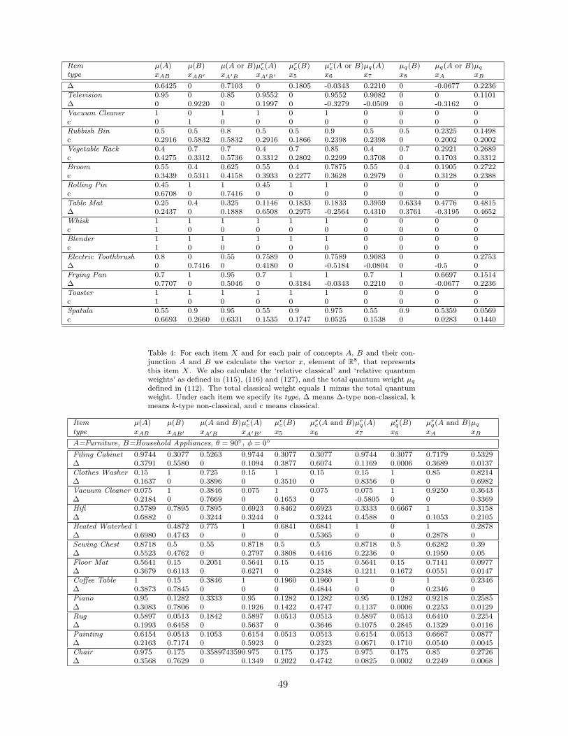
Item µ(A) µ(B) µ(A or B)µrc(A) µrc(B) µrc(A or B)µq(A) µq(B) µq(A or B)µqtype xAB xAB′ xA′B xA′B′ x5 x6 x7 x8 xA xB

∆ 0.6425 0 0.7103 0 0.1805 -0.0343 0.2210 0 -0.0677 0.2236Television 0.95 0 0.85 0.9552 0 0.9552 0.9082 0 0 0.1101∆ 0 0.9220 0 0.1997 0 -0.3279 -0.0509 0 -0.3162 0Vacuum Cleaner 1 0 1 1 0 1 0 0 0 0c 0 1 0 0 0 0 0 0 0 0Rubbish Bin 0.5 0.5 0.8 0.5 0.5 0.9 0.5 0.5 0.2325 0.1498c 0.2916 0.5832 0.5832 0.2916 0.1866 0.2398 0.2398 0 0.2002 0.2002Vegetable Rack 0.4 0.7 0.7 0.4 0.7 0.85 0.4 0.7 0.2921 0.2689c 0.4275 0.3312 0.5736 0.3312 0.2802 0.2299 0.3708 0 0.1703 0.3312Broom 0.55 0.4 0.625 0.55 0.4 0.7875 0.55 0.4 0.1905 0.2722c 0.3439 0.5311 0.4158 0.3933 0.2277 0.3628 0.2979 0 0.3128 0.2388Rolling Pin 0.45 1 1 0.45 1 1 0 0 0 0c 0.6708 0 0.7416 0 0 0 0 0 0 0Table Mat 0.25 0.4 0.325 0.1146 0.1833 0.1833 0.3959 0.6334 0.4776 0.4815∆ 0.2437 0 0.1888 0.6508 0.2975 -0.2564 0.4310 0.3761 -0.3195 0.4652Whisk 1 1 1 1 1 1 0 0 0 0c 1 0 0 0 0 0 0 0 0 0Blender 1 1 1 1 1 1 0 0 0 0c 1 0 0 0 0 0 0 0 0 0Electric Toothbrush 0.8 0 0.55 0.7589 0 0.7589 0.9083 0 0 0.2753∆ 0 0.7416 0 0.4180 0 -0.5184 -0.0804 0 -0.5 0Frying Pan 0.7 1 0.95 0.7 1 1 0.7 1 0.6697 0.1514∆ 0.7707 0 0.5046 0 0.3184 -0.0343 0.2210 0 -0.0677 0.2236Toaster 1 1 1 1 1 1 0 0 0 0c 1 0 0 0 0 0 0 0 0 0Spatula 0.55 0.9 0.95 0.55 0.9 0.975 0.55 0.9 0.5359 0.0569c 0.6693 0.2660 0.6331 0.1535 0.1747 0.0525 0.1538 0 0.0283 0.1440

Table 4: For each item X and for each pair of concepts A, B and their con-junction A and B we calculate the vector x, element of R8, that representsthis item X. We also calculate the ‘relative classical’ and ‘relative quantumweights’ as defined in (115), (116) and (127), and the total quantum weight µqdefined in (112). The total classical weight equals 1 minus the total quantumweight. Under each item we specify its type, ∆ means ∆-type non-classical, kmeans k-type non-classical, and c means classical.

Item µ(A) µ(B) µ(A and B)µrc(A) µrc(B) µrc(A and B)µrq(A) µrq(B) µrq(A and B)µqtype xAB xAB′ xA′B xA′B′ x5 x6 x7 x8 xA xB

A=Furniture, B=Household Appliances, θ = 90, φ = 0

Filing Cabinet 0.9744 0.3077 0.5263 0.9744 0.3077 0.3077 0.9744 0.3077 0.7179 0.5329∆ 0.3791 0.5580 0 0.1094 0.3877 0.6074 0.1169 0.0006 0.3689 0.0137Clothes Washer 0.15 1 0.725 0.15 1 0.15 0.15 1 0.85 0.8214∆ 0.1637 0 0.3896 0 0.3510 0 0.8356 0 0 0.6982Vacuum Cleaner 0.075 1 0.3846 0.075 1 0.075 0.075 1 0.9250 0.3643∆ 0.2184 0 0.7669 0 0.1653 0 -0.5805 0 0 0.3369Hifi 0.5789 0.7895 0.7895 0.6923 0.8462 0.6923 0.3333 0.6667 1 0.3158∆ 0.6882 0 0.3244 0.3244 0 0.3244 0.4588 0 0.1053 0.2105Heated Waterbed 1 0.4872 0.775 1 0.6841 0.6841 1 0 1 0.2878∆ 0.6980 0.4743 0 0 0 0.5365 0 0 0.2878 0Sewing Chest 0.8718 0.5 0.55 0.8718 0.5 0.5 0.8718 0.5 0.6282 0.39∆ 0.5523 0.4762 0 0.2797 0.3808 0.4416 0.2236 0 0.1950 0.05Floor Mat 0.5641 0.15 0.2051 0.5641 0.15 0.15 0.5641 0.15 0.7141 0.0977∆ 0.3679 0.6113 0 0.6271 0 0.2348 0.1211 0.1672 0.0551 0.0147Coffee Table 1 0.15 0.3846 1 0.1960 0.1960 1 0 1 0.2346∆ 0.3873 0.7845 0 0 0 0.4844 0 0 0.2346 0Piano 0.95 0.1282 0.3333 0.95 0.1282 0.1282 0.95 0.1282 0.9218 0.2585∆ 0.3083 0.7806 0 0.1926 0.1422 0.4747 0.1137 0.0006 0.2253 0.0129Rug 0.5897 0.0513 0.1842 0.5897 0.0513 0.0513 0.5897 0.0513 0.6410 0.2254∆ 0.1993 0.6458 0 0.5637 0 0.3646 0.1075 0.2845 0.1329 0.0116Painting 0.6154 0.0513 0.1053 0.6154 0.0513 0.0513 0.6154 0.0513 0.6667 0.0877∆ 0.2163 0.7174 0 0.5923 0 0.2323 0.0671 0.1710 0.0540 0.0045Chair 0.975 0.175 0.3589743590.975 0.175 0.175 0.975 0.175 0.85 0.2726∆ 0.3568 0.7629 0 0.1349 0.2022 0.4742 0.0825 0.0002 0.2249 0.0068

49

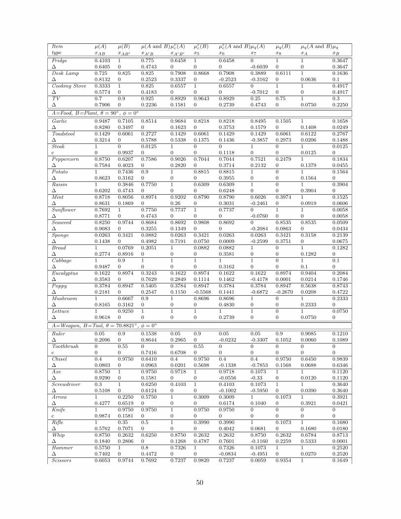
Item µ(A) µ(B) µ(A and B)µrc(A) µrc(B) µrc(A and B)µq(A) µq(B) µq(A and B)µqtype xAB xAB′ xA′B xA′B′ x5 x6 x7 x8 xA xB

Fridge 0.4103 1 0.775 0.6458 1 0.6458 0 1 1 0.3647∆ 0.6405 0 0.4743 0 0 0 -0.6039 0 0 0.3647Desk Lamp 0.725 0.825 0.825 0.7908 0.8668 0.7908 0.3889 0.6111 1 0.1636∆ 0.8132 0 0.2523 0.3337 0 -0.2523 -0.3162 0 0.0636 0.1Cooking Stove 0.3333 1 0.825 0.6557 1 0.6557 0 1 1 0.4917∆ 0.5774 0 0.4183 0 0 0 -0.7012 0 0 0.4917TV 0.7 0.9 0.925 0.8929 0.9643 0.8929 0.25 0.75 1 0.3∆ 0.7906 0 0.2236 0.1581 0 0.2739 0.4743 0 0.0750 0.2250

A=Food, B=Plant, θ = 90, φ = 0

Garlic 0.9487 0.7105 0.8514 0.9684 0.8218 0.8218 0.8495 0.1505 1 0.1658∆ 0.8280 0.3497 0 0.1623 0 0.3753 0.1579 0 0.1408 0.0249Toadstool 0.1429 0.6061 0.2727 0.1429 0.6061 0.1429 0.1429 0.6061 0.6122 0.2767∆ 0.3214 0 0.5788 0.5338 0.1375 0.1436 -0.3857 0.2973 0.0206 0.1488Steak 1 0 0.0125 1 0 0 1 0 1 0.0125c 0 0.9937 0 0 0 0.1118 0 0 0.0125 0Peppercorn 0.8750 0.6207 0.7586 0.9026 0.7044 0.7044 0.7521 0.2479 1 0.1834∆ 0.7584 0.4023 0 0.2820 0 0.3714 0.2132 0 0.1379 0.0455Potato 1 0.7436 0.9 1 0.8815 0.8815 1 0 1 0.1564∆ 0.8623 0.3162 0 0 0 0.3955 0 0 0.1564 0Raisin 1 0.3846 0.7750 1 0.6309 0.6309 1 0 1 0.3904∆ 0.6202 0.4743 0 0 0 0.6248 0 0 0.3904 0Mint 0.8718 0.8056 0.8974 0.9202 0.8790 0.8790 0.6026 0.3974 1 0.1525∆ 0.8631 0.1869 0 0.26 0 0.3031 -0.2461 0 0.0919 0.0606Sunflower 0.7692 1 0.7750 0.7737 1 0.7737 0 1 1 0.0058∆ 0.8771 0 0.4743 0 0 0 -0.0760 0 0 0.0058Seaweed 0.8250 0.9744 0.8684 0.8692 0.9808 0.8692 0 0.8535 0.8535 0.0509∆ 0.9083 0 0.3255 0.1349 0 0 -0.2084 0.0863 0 0.0434Sponge 0.0263 0.3421 0.0882 0.0263 0.3421 0.0263 0.0263 0.3421 0.3158 0.2139∆ 0.1438 0 0.4982 0.7191 0.0750 0.0009 -0.2599 0.3751 0 0.0675Bread 1 0.0769 0.2051 1 0.0882 0.0882 1 0 1 0.1282∆ 0.2774 0.8916 0 0 0 0.3581 0 0 0.1282 0Cabbage 1 0.9 1 1 1 1 1 0 1 0.1∆ 0.9487 0 0 0 0 0.3162 0 0 0.1 0Eucalyptus 0.1622 0.8974 0.3243 0.1622 0.8974 0.1622 0.1622 0.8974 0.9404 0.2084∆ 0.3583 0 0.7629 0.2849 0.1114 0.1462 -0.4178 0.0001 0.0214 0.1746Poppy 0.3784 0.8947 0.5405 0.3784 0.8947 0.3784 0.3784 0.8947 0.5638 0.8743∆ 0.2181 0 0.2547 0.1150 -0.5568 0.1441 -0.6872 -0.2670 0.0208 0.4722Mushroom 1 0.6667 0.9 1 0.8696 0.8696 1 0 1 0.2333∆ 0.8165 0.3162 0 0 0 0.4830 0 0 0.2333 0Lettuce 1 0.9250 1 1 1 1 1 0 1 0.0750∆ 0.9618 0 0 0 0 0.2739 0 0 0.0750 0

A=Weapon, B=Tool, θ = 70.8821, φ = 0

Ruler 0.05 0.9 0.1538 0.05 0.9 0.05 0.05 0.9 0.9085 0.1210∆ 0.2096 0 0.8644 0.2965 0 -0.0232 -0.3307 0.1052 0.0060 0.1089Toothbrush 0 0.55 0 0 0.55 0 0 0 0 0c 0 0 0.7416 0.6708 0 0 0 0 0 0Chisel 0.4 0.9750 0.6410 0.4 0.9750 0.4 0.4 0.9750 0.6450 0.9839∆ 0.0803 0 0.0963 0.0201 0.5698 -0.1338 -0.7853 0.1568 0.0688 0.6346Axe 0.8750 1 0.9750 0.9718 1 0.9718 0.1073 1 1 0.1120∆ 0.9290 0 0.1581 0 0 -0.0556 -0.33 0 0.0120 0.1120Screwdriver 0.3 1 0.6250 0.4103 1 0.4103 0.1073 1 1 0.3640∆ 0.5108 0 0.6124 0 0 -0.1002 -0.5950 0 0.0390 0.3640Arrow 1 0.2250 0.5750 1 0.3009 0.3009 1 0.1073 1 0.3921∆ 0.4277 0.6519 0 0 0 0.6174 0.1040 0 0.3921 0.0421Knife 1 0.9750 0.9750 1 0.9750 0.9750 0 0 0 0c 0.9874 0.1581 0 0 0 0 0 0 0 0Rifle 1 0.35 0.5 1 0.3990 0.3990 1 0.1073 1 0.1680∆ 0.5762 0.7071 0 0 0 0.4042 0.0681 0 0.1680 0.0180Whip 0.8750 0.2632 0.6250 0.8750 0.2632 0.2632 0.8750 0.2632 0.6784 0.8713∆ 0.1840 0.2806 0 0.1268 0.4787 0.7601 -0.1160 0.2259 0.5333 0.0001Hammer 0.5750 1 0.8 0.7326 1 0.7326 0.1073 1 1 0.2520∆ 0.7402 0 0.4472 0 0 -0.0834 -0.4951 0 0.0270 0.2520Scissors 0.6053 0.9744 0.7692 0.7237 0.9820 0.7237 0.0059 0.9354 1 0.1649

50

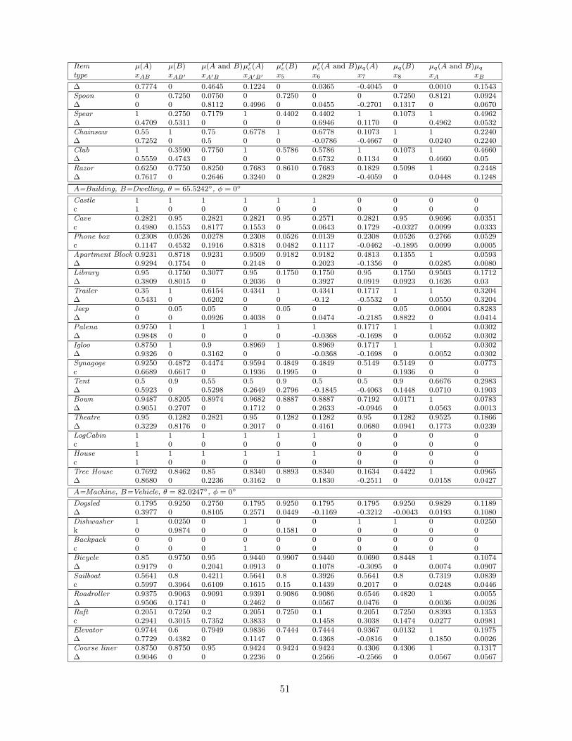
Item µ(A) µ(B) µ(A and B)µrc(A) µrc(B) µrc(A and B)µq(A) µq(B) µq(A and B)µqtype xAB xAB′ xA′B xA′B′ x5 x6 x7 x8 xA xB

∆ 0.7774 0 0.4645 0.1224 0 0.0365 -0.4045 0 0.0010 0.1543Spoon 0 0.7250 0.0750 0 0.7250 0 0 0.7250 0.8121 0.0924∆ 0 0 0.8112 0.4996 0 0.0455 -0.2701 0.1317 0 0.0670Spear 1 0.2750 0.7179 1 0.4402 0.4402 1 0.1073 1 0.4962∆ 0.4709 0.5311 0 0 0 0.6946 0.1170 0 0.4962 0.0532Chainsaw 0.55 1 0.75 0.6778 1 0.6778 0.1073 1 1 0.2240∆ 0.7252 0 0.5 0 0 -0.0786 -0.4667 0 0.0240 0.2240Club 1 0.3590 0.7750 1 0.5786 0.5786 1 0.1073 1 0.4660∆ 0.5559 0.4743 0 0 0 0.6732 0.1134 0 0.4660 0.05Razor 0.6250 0.7750 0.8250 0.7683 0.8610 0.7683 0.1829 0.5098 1 0.2448∆ 0.7617 0 0.2646 0.3240 0 0.2829 -0.4059 0 0.0448 0.1248

A=Building, B=Dwelling, θ = 65.5242, φ = 0

Castle 1 1 1 1 1 1 0 0 0 0c 1 0 0 0 0 0 0 0 0 0Cave 0.2821 0.95 0.2821 0.2821 0.95 0.2571 0.2821 0.95 0.9696 0.0351c 0.4980 0.1553 0.8177 0.1553 0 0.0643 0.1729 -0.0327 0.0099 0.0333Phone box 0.2308 0.0526 0.0278 0.2308 0.0526 0.0139 0.2308 0.0526 0.2766 0.0529c 0.1147 0.4532 0.1916 0.8318 0.0482 0.1117 -0.0462 -0.1895 0.0099 0.0005Apartment Block 0.9231 0.8718 0.9231 0.9509 0.9182 0.9182 0.4813 0.1355 1 0.0593∆ 0.9294 0.1754 0 0.2148 0 0.2023 -0.1356 0 0.0285 0.0080Library 0.95 0.1750 0.3077 0.95 0.1750 0.1750 0.95 0.1750 0.9503 0.1712∆ 0.3809 0.8015 0 0.2036 0 0.3927 0.0919 0.0923 0.1626 0.03Trailer 0.35 1 0.6154 0.4341 1 0.4341 0.1717 1 1 0.3204∆ 0.5431 0 0.6202 0 0 -0.12 -0.5532 0 0.0550 0.3204Jeep 0 0.05 0.05 0 0.05 0 0 0.05 0.0604 0.8283∆ 0 0 0.0926 0.4038 0 0.0474 -0.2185 0.8822 0 0.0414Palena 0.9750 1 1 1 1 1 0.1717 1 1 0.0302∆ 0.9848 0 0 0 0 -0.0368 -0.1698 0 0.0052 0.0302Igloo 0.8750 1 0.9 0.8969 1 0.8969 0.1717 1 1 0.0302∆ 0.9326 0 0.3162 0 0 -0.0368 -0.1698 0 0.0052 0.0302Synagoge 0.9250 0.4872 0.4474 0.9594 0.4849 0.4849 0.5149 0.5149 0 0.0773c 0.6689 0.6617 0 0.1936 0.1995 0 0 0.1936 0 0Tent 0.5 0.9 0.55 0.5 0.9 0.5 0.5 0.9 0.6676 0.2983∆ 0.5923 0 0.5298 0.2649 0.2796 -0.1845 -0.4063 0.1448 0.0710 0.1903Bown 0.9487 0.8205 0.8974 0.9682 0.8887 0.8887 0.7192 0.0171 1 0.0783∆ 0.9051 0.2707 0 0.1712 0 0.2633 -0.0946 0 0.0563 0.0013Theatre 0.95 0.1282 0.2821 0.95 0.1282 0.1282 0.95 0.1282 0.9525 0.1866∆ 0.3229 0.8176 0 0.2017 0 0.4161 0.0680 0.0941 0.1773 0.0239LogCabin 1 1 1 1 1 1 0 0 0 0c 1 0 0 0 0 0 0 0 0 0House 1 1 1 1 1 1 0 0 0 0c 1 0 0 0 0 0 0 0 0 0Tree House 0.7692 0.8462 0.85 0.8340 0.8893 0.8340 0.1634 0.4422 1 0.0965∆ 0.8680 0 0.2236 0.3162 0 0.1830 -0.2511 0 0.0158 0.0427

A=Machine, B=Vehicle, θ = 82.0247, φ = 0

Dogsled 0.1795 0.9250 0.2750 0.1795 0.9250 0.1795 0.1795 0.9250 0.9829 0.1189∆ 0.3977 0 0.8105 0.2571 0.0449 -0.1169 -0.3212 -0.0043 0.0193 0.1080Dishwasher 1 0.0250 0 1 0 0 1 1 0 0.0250k 0 0.9874 0 0 0.1581 0 0 0 0 0Backpack 0 0 0 0 0 0 0 0 0 0c 0 0 0 1 0 0 0 0 0 0Bicycle 0.85 0.9750 0.95 0.9440 0.9907 0.9440 0.0690 0.8448 1 0.1074∆ 0.9179 0 0.2041 0.0913 0 0.1078 -0.3095 0 0.0074 0.0907Sailboat 0.5641 0.8 0.4211 0.5641 0.8 0.3926 0.5641 0.8 0.7319 0.0839c 0.5997 0.3964 0.6109 0.1615 0.15 0.1439 0.2017 0 0.0248 0.0446Roadroller 0.9375 0.9063 0.9091 0.9391 0.9086 0.9086 0.6546 0.4820 1 0.0055∆ 0.9506 0.1741 0 0.2462 0 0.0567 0.0476 0 0.0036 0.0026Raft 0.2051 0.7250 0.2 0.2051 0.7250 0.1 0.2051 0.7250 0.8393 0.1353c 0.2941 0.3015 0.7352 0.3833 0 0.1458 0.3038 0.1474 0.0277 0.0981Elevator 0.9744 0.6 0.7949 0.9836 0.7444 0.7444 0.9367 0.0132 1 0.1975∆ 0.7729 0.4382 0 0.1147 0 0.4368 -0.0816 0 0.1850 0.0026Course liner 0.8750 0.8750 0.95 0.9424 0.9424 0.9424 0.4306 0.4306 1 0.1317∆ 0.9046 0 0 0.2236 0 0.2566 -0.2566 0 0.0567 0.0567

51

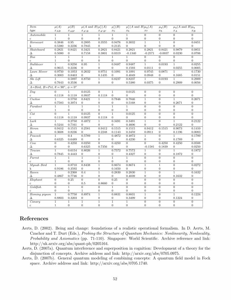
Item µ(A) µ(B) µ(A and B)µrc(A) µrc(B) µrc(A and B)µq(A) µq(B) µq(A and B)µqtype xAB xAB′ xA′B xA′B′ x5 x6 x7 x8 xA xB

Automobile 1 1 1 1 1 1 0 0 0 0c 1 0 0 0 0 0 0 0 0 0Horsecart 0.3846 0.95 0.2895 0.3555 0.9476 0.3032 1 1 0 0.0451k 0.5380 0.2236 0.7845 0 0.2125 0 0 0 0 0Skateboard 0.2821 0.8421 0.3421 0.2821 0.8421 0.2821 0.2821 0.8421 0.9879 0.0851∆ 0.5080 0 0.7158 0.3801 0.0319 -0.1340 -0.2571 -0.0037 0.0230 0.0706Bus 1 1 1 1 1 1 0 0 0 0c 1 0 0 0 0 0 0 0 0 0Bulldozer 1 0.9250 0.95 1 0.9487 0.9487 1 0.0193 1 0.0255∆ 0.9615 0.2236 0 0 0 0.1593 0.0111 0 0.0255 0.0005Lawn Mover 0.9750 0.1053 0.2632 0.9751 0.1091 0.1091 0.9745 0.0871 1 0.1730∆ 0.3003 0.8463 0 0.1435 0 0.4049 0.0948 0 0.1685 0.0151Ski Lift 1 0.5897 0.8750 1 0.8237 0.8237 1 0.0193 1 0.2909∆ 0.7643 0.3536 0 0 0 0.5380 0.0375 0 0.2909 0.0056

A=Bird, B=Pet, θ = 90, φ = 0

Dog 0 1 0.0125 0 1 0.0125 0 0 0 0c 0.1118 0.1118 0.9937 0.1118 0 0 0 0 0 0Cuckoo 1 0.5750 0.8421 1 0.7846 0.7846 1 0 1 0.2671∆ 0.7583 0.3974 0 0 0 0.5168 0 0 0.2671 0Parakeet 1 1 1 1 1 1 0 0 0 0c 1 0 0 0 0 0 0 0 0 0Cat 0 1 0.0125 0 1 0.0125 0 0 0 0c 0.1118 0.1118 0.9937 0.1118 0 0 0 0 0 0Lark 1 0.2750 0.4872 1 0.3491 0.3491 1 0 1 0.2122∆ 0.5244 0.7161 0 0 0 0.4606 0 0 0.2122 0Heron 0.9412 0.1515 0.2581 0.9412 0.1515 0.1515 0.9412 0.1515 0.9073 0.1410∆ 0.3608 0.8236 0 0.2248 0.1143 0.3459 0.0911 0 0.1196 0.0083Peacock 1 0.4 0.5789 1 0.4872 0.4872 1 0 1 0.1789∆ 0.6325 0.6489 0 0 0 0.4230 0 0 0.1789 0Cow 0 0.4250 0.0250 0 0.4250 0 0 0.4250 0.4250 0.0588∆ 0 0 0.6325 0.7356 0 0 -0.1581 0.1839 0 0.0250Toucan 1 0.6154 0.8026 1 0.7572 0.7572 1 0 1 0.1872∆ 0.7845 0.4443 0 0 0 0.4327 0 0 0.1872 0Parrot 1 1 1 1 1 1 0 0 0 0c 1 0 0 0 0 0 0 0 0 0Mynah Bird 1 0.8710 0.8438 1 0.8674 0.8674 1 1 0 0.0272k 0.9186 0.3592 0 0 0.1650 0 0 0 0 0Raven 1 0.2368 0.4 1 0.2830 0.2830 1 0 1 0.1632∆ 0.4867 0.7746 0 0 0 0.4039 0 0 0.1632 0Elephant 0 0.25 0 0 0.25 0 0 0 0 0c 0 0 0.5 0.8660 0 0 0 0 0 0Goldfish 0 1 0 0 1 0 0 0 0 0c 0 0 1 0 0 0 0 0 0 0Homing pigeon 1 0.7750 0.8974 1 0.8831 0.8831 1 0 1 0.1224∆ 0.8803 0.3203 0 0 0 0.3499 0 0 0.1224 0Canary 1 1 1 1 1 1 0 0 0 0c 1 0 0 0 0 0 0 0 0 0

References

Aerts, D. (2002). Being and change: foundations of a realistic operational formalism. In D. Aerts, M.Czachor and T. Durt (Eds.), Probing the Structure of Quantum Mechanics: Nonlinearity, Nonlocality,Probability and Axiomatics (pp. 71-110). Singapore: World Scientific. Archive reference and link:http://uk.arxiv.org/abs/quant-ph/0205164.

Aerts, D. (2007a). Quantum interference and superposition in cognition: Development of a theory for thedisjunction of concepts. Archive address and link: http://arxiv.org/abs/0705.0975.

Aerts, D. (2007b). General quantum modeling of combining concepts: A quantum field model in Fockspace. Archive address and link: http://arxiv.org/abs/0705.1740.

52

Aerts, D., & Aerts, S. (1994). Applications of quantum statistics in psychological studies of decisionprocesses. Foundations of Science, 1, 85-97. Reprinted in B. Van Fraassen (1997), (Eds.), Topics inthe Foundation of Statistics (pp. 111-122). Dordrecht: Kluwer Academic.

Aerts, S. and Aerts, D. (2008). When can a data set be described by quantum theory? In P. Bruza,W. Lawless, K. van Rijsbergen, D. Sofge, B. Coecke and S. Clark (Eds.), Proceedings of the SecondQuantum Interaction Symposium, Oxford 2008, pp. 27-33. London: College Publications.

Aerts, D., Aerts, S. & Gabora, L. (2009). Experimental evidence for quantum structure in cognition.In Bruza P.D., Sofge D., Lawless, W., Van Rijsbergen, C.J., Klusch, M. (Eds.). Proceedings of QI2009-Third International Symposium on Quantum Interaction, Lecture Notes in Computer Science.Berlin: Springer.

Aerts, D. & D’Hooghe, B. (2009). Classical logical versus quantum conceptual thought: Examples ineconomics, decision theory and concept theory. In Bruza P.D., Sofge D., Lawless, W., Van Rijsber-gen, C.J., Klusch, M. (Eds.). Proceedings of QI 2009-Third International Symposium on QuantumInteraction, Lecture Notes in Computer Science. Berlin: Springer.

Aerts, D., & Czachor, M. (2004). Quantum aspects of semantic analysis and symbolic artificial intelligence.Journal of Physics A, Mathematical and Theoretical, 37, L123-L132.

Aerts, D., Czachor, M. and D’Hooghe, B. (2006). Towards a quantum evolutionary scheme: violatingBell’s inequalities in language. In N. Gontier, J. P. Van Bendegem and D. Aerts (Eds.), EvolutionaryEpistemology, Language and Culture - A non adaptationist systems theoretical approach. Dordrecht:Springer.

Aerts, D., & Gabora, L. (2005a). A theory of concepts and their combinations II: A Hilbert spacerepresentation. Kybernetes, 34, 192-221.

Aerts, D., & Gabora, L. (2005b). A theory of concepts and their combinations I: The structure of thesets of contexts and properties. Kybernetes, 34, 167-191.

Allais, M. (1953). Le comportement de l’homme rationnel devant le risque: critique des postulats etaxiomes de l’ecole Americaine. Econometrica, 21, 503-546.

Baaquie, B. E. (2004). Quantum Finance: Path Integrals and Hamiltonians for Options and InterestRates. Cambridge UK: Cambridge University Press.

Bagassi, M., Macchi, L. (2007). The ‘vanishing’ of the disjunction effect by sensible procrastination. Mind& Society 6, 4152.

Barsalou, L. (1987). The instability of graded structure: Implications of the nature of concepts. In U.Neisser (Eds.), Concepts and Conceptual Development: Ecological and Intellectual factors in Catego-rization. Cambridge: Cambridge University Press.

Berry, M. W., Dumais, S. T., and O’Brien, G. W. (1995). Using linear algebra for intelligent informationretrieval. SIAM Review, 37, 573-595.

Bruner, J. (1990). Acts of Meaning. Cambridge, MA: Harvard University Press.Bruza, P. D. and Cole, R. J. (2005). Quantum logic of semantic space: An exploratory investigation of

context effects in practical reasoning. In S. Artemov, H. Barringer, A. S. d’Avila Garcez, L.C. Lamb,J. Woods (Eds.) We Will Show Them: Essays in Honour of Dov Gabbay. College Publications.

Bruza, P.D., Kitto, K., Nelson, D. and McEvoy, K. (2008). Entangling words and meaning. Proceedingsof the Second Quantum Interaction Symposium, University of Oxford.

Bruza, P.D., Kitto, K., Nelson D. and McEvoy, C. (2009). Extracting spooky-activation-at-a-distancefrom considerations of entanglement, In Bruza P.D., Sofge D., Lawless, W., Van Rijsbergen, C.J.,Klusch, M. (Eds.). Proceedings of QI 2009-Third International Symposium on Quantum Interaction,Lecture Notes in Computer Science. Berlin: Springer.

Bruza, P.D., Widdows, D. & Woods J.H. (in press). A Quantum logic of down below. In Handbook ofQuantum Logic and Quantum Structures. Volume 2. Elsevier.

Busemeyer, J. R., Wang, Z., & Townsend, J. T. (2006). Quantum dynamics of human decision making.Journal of Mathematical Psychology, 50, 220-241.

53

Busemeyer, J. R., Matthew, M., Wang, Z. (2006) A Quantum Information Processing Theory Explanationof Disjunction Effects. Proceedings of the Cognitive Science Society.

Deerwester, S., Dumais, S. T. & Harshman, R. (1990). Indexing by Latent Semantic Analysis. Journalof the Society for Information Science, 41, 391-407.

Dirac, P. A. M. (1958). Quantum mechanics, 4th ed. London: Oxford University Press.Ellsberg, D. (1961). Risk, Ambiguity, and the Savage Axioms. Quarterly Journal of Economics, 75,

643-669.Flender, C., Kitto, K. & Bruza, P. D. (2009). Beyond ontology in information systems. In Bruza, P., Sofge,

D., Lawless, W., Rijsbergen, K., Klusch, M. (Eds.). Proceedings of the Third Quantum InteractionSymposium. Volume 5494 of Lecture Notes in Artificial Intelligence, Springer.

Fodor, J. (1975). The Language of Thought. New York: Thomas Crowell.Franco, R. (2007). Quantum mechanics, Bayes’ theorem and the conjunction fallacy. Archive address and

link: http://arxiv.org/abs/0708.3948Freud, S. (1899). Die Traumdeutung. Berlin: Fischer-Taschenbuch.Gabora, L., & Aerts, D. (2002a). Contextualizing concepts. In Proceedings of the 15th International

FLAIRS Conference. Special track: Categorization and Concept Representation: Models and Impli-cations, Pensacola Florida, May 14-17, American Association for Artificial Intelligence (pp. 148-152).

Gabora, L., & Aerts, D. (2002b). Contextualizing concepts using a mathematical generalization of thequantum formalism. Journal of Experimental and Theoretical Artificial Intelligence, 14, 327-358.Preprint at http://arXiv.org/abs/quant-ph/0205161

Gabora, L., Rosch, E., Aerts, D. (2008). Toward an ecological theory of concepts. Eco- logical Psychology20, 84116.

Gardenfors, P. (2004). Conceptual Spaces: The Geometry of Thought. Boston, USA: MIT-Press.Hampton, J. A. (1987). Inheritance of attributes in natural concept conjunctions. Memory & Cognition,

15, 55-71.Hampton, J. A. (1988a). Overextension of conjunctive concepts: Evidence for a unitary model for con-

cept typicality and class inclusion. Journal of Experimental Psychology: Learning, Memory, andCognition, 14, 12-32.

Hampton, J. A. (1988b). Disjunction of natural concepts. Memory & Cognition, 16, 579-591.Hampton, J. A. (1991). The combination of prototype concepts. In P. Schwanenflugel (Ed.), The Psy-

chology of Word Meanings. Hillsdale, NJ: Erlbaum.Hampton, J. A. (1993). Prototype models of concept representation. In I. Van Mechelen, J. Hampton, R.

S. Michalski, & P. Theuns (Eds.), Categories and Concepts: Theoretical Views and Inductive DataAnalysis (pp. 67-95). London, UK: Academic Press.

Hampton, J.A. (1996). Conjunctions of visually-based categories: overextension and compensation. Jour-nal of Experimental Psychology: Learning, Memory and Cognition, 22, 378-396.

Hampton, J. A. (1997a). Conceptual combination: Conjunction and negation of natural concepts. Mem-ory & Cognition, 25, 888-909.

Hampton, J. A. (1997b). Conceptual combination. In K. Lamberts & D. Shanks (Eds.), Knowledge,Concepts, and Categories (pp. 133-159). Hove: Psychology Press.

Haven, E. (2005). Pilot-wave theory and financial option pricing. International Journal of TheoreticalPhysics, 44, 1957-1962.

Hettel, T., Flender, C., Barros, A.: Scaling Choreography Modelling for B2B Value- Chain Analysis. In:Proceeding of the 6th International Conference on Business Process Management (BPM 2008), 1-4September 2008, Milan, Italy. (2008)

James, W. (1910). Some Problems of Philosophy. Cambridge, MA: Harvard University Press.Komatsu, L. K. (1992). Recent views of conceptual structure. Psychological Bulletin, 112, 500-526.Kolmogorov, A. N. (1977). Grundbegriffe der Wahrscheinlichkeitsrechnung. Reprint der Erstauflage Berlin

1933. Berlin: Springer.

54

Khrennikov, A. (2008). A model of quantum-like decision-making with applications to psychology andcognitive science. Archive address and link: http://uk.arxiv.org/abs/0711.1366

Khrennikov, A. (2009). Design of an experiment to test quantum probabilistic behavior of the financialmarket. http://uk.arxiv.org/abs/0902.1922

Kunda, Z., Miller, D. T., & Claire, T. (1990). Combining social concepts: The role of causal reasoning.Cognitive Science, 14, 551-577.

Landauer, T. K., Foltz, P. W. and Laham, D. (1998). Introduction to Latent Semantic Analysis. DiscourseProcesses 25, 259-284.

Lund, K & Burgess, C. (1996). Producing high-dimensional semantic spaces from lexical co-occurrence.Behavior Research Methods, Instruments and Computers, 28, 203-208.

Margolis, E. and Laurence, S. (2002). Radical concept nativism. Cognition, 86, 25-55.Nelson, D. L. & McEvoy, C. L. (2007). Entangled associative structures and context. In P. Bruza, W.

Lawless, K. van Rijsbergen, & D. Sofge (Eds.) Proceedings of the Association for the Advancementof Artificial Intelligence (AAAI) Spring Symposium 8: Quantum Interaction, March 26-28, 2007,Stanford University.

Osherson , D. N. & Smith, E. E. (1981). On the adequacy of prototype theory as a theory of concepts.Cognition, 9, 35-58.

Osherson, D. N. & Smith, E. E. (1982). Gradedness and conceptual combination. Cognition, 12, 299-318.Piaget, J. (1990). Le Langage et la Pensee Chez l’Enfant. Paris: Delachaux et Niestle.Pitowsky, I. (1989). Quantum Probability, Quantum Logic. Lecture Notes in Physics 321. Heidelberg:

Springer.Rips, L J. (1995). The current status of research on concept combination. Mind & Language, 10, 72-104.Rosch, E. (1973a). Natural categories. Cognitive Psychology, 4, 328.Rosch, E. (1973b). On the internal structure of perceptual and semantic categories. In T. E. Moore (Ed.),

Cognitive Development and the Acquisition of Language. New York: Academic Press.Savage, L.J. (1944). The Foundations of Statistics. New-York: Wiley.Schaden, M. (2002). Quantum finance: A quantum approach to stock price fluctuations. Physica A, 316,

511-538.Smith, E. E., & Medin, D. L. (1981). Categories and Concepts. Cambridge, MA.: Harvard University

Press.Smith, E. E., & Osherson, D. N. (1984). Conceptual combination with prototype concepts. Cognitive

Science, 8, 357-361.Smith, E. E., Osherson, D. N., Rips, L. J., & Keane, M. (1988). Combining prototypes: A selective

modification model. Cognitive Science, 12, 485-527.Smolensky, P. (1990). Tensor product variable binding and the representation of symbolic structures in

connectionist systems. Artificial Intelligence, 46, 159-216.Springer, K., & Murphy, G. L. (1992). Feature availability in conceptual combination. Psychological

Science, 3, 111-117.Storms, G., De Boeck, P., Van Mechelen, I., & Geeraerts, D. (1993). Dominance and non-commutativity

effects in concept conjunctions: Extensional or intensional basis? Memory & Cognition, 21, 752-762.Storms, G., de Boeck, P., Hampton, J.A., & van Mechelen, I. (1999). Predicting conjunction typicalities

by component typicalities. Psychonomic Bulletin and Review, 6, 677-684.Tversky, A. & Kahneman, D. (1982). Judgments of and by representativeness. In D. Kahneman, P.

Slovic & A. Tversky (Eds.), Judgment under uncertainty: Heuristics and biases. Cambridge, UK:Cambridge University Press.

Tversky, A. & Shafir, E. (1992). The disjunction effect in choice under uncertainty. Psychological Science,3, 305-309.

Van Rijsbergen, K. (2004). The Geometry of Information Retrieval. Cambridge UK: Cambridge Univer-sity Press.

55

Widdows, D. (2003). Orthogonal negation in vector spaces for modelling word-meanings and documentretrieval. In Proceedings of the 41st Annual Meeting of the Association for Computational Linguistics(pp. 136-143). Sapporo, Japan, July 7-12.

Widdows, D. (2006). Geometry and Meaning. CSLI Publications: University of Chicago Press.Widdows, D., & Peters, S. (2003). Word vectors and quantum logic: Experiments with negation and

disjunction. In Mathematics of Language 8 (pp. 141-154). Indiana: Bloomington.Zadeh, L. (1965). Fuzzy sets. Information & Control, 8, 338-353.

A Appendix: Proof of Theorem 1:

If µ(A), µ(B) and µ(A and B) are classical conjunction data, there exists a Kolmogorovian probabilityspace (Ω, σ(Ω), P ) and events EA, EB ∈ σ(Ω) such that P (EA) = µ(A), P (EB) = µ(B) and P (EA∩EB) =µ(A and B). From the general properties of a Kolmogorovian probability space it follows that we have0 ≤ P (EA ∩ EB) ≤ P (EA) ≤ 1 and 0 ≤ P (EA ∩ EB) ≤ P (EB) ≤ 1, which proves that inequalities (4) and(5) are satisfied. From the same general properties of a Kolmogorovian probability space it also followsthat we have P (EA ∪ EB) = P (EA) + P (EB) − P (EA ∩ EB), and since P (EA ∪ EB) ≤ 1 we also haveP (EA) + P (EB) − P (EA ∩ EB) ≤ 1. This proves that inequality (6) is satisfied. We have now provedthat for classical conjunction data µ(A), µ(B) and µ(A and B) the three inequalities are satisfied. Nowsuppose that we have an item X such that for its membership weights µ(A), µ(B), µ(A and B) with respectto concepts A and B and their conjunction ‘A and B’, inequalities (4), (5) and (6) are satisfied. We willprove that as a consequence µ(A), µ(B) and µ(A and B) are classical conjunction data. To this end,we will explicitly construct a Kolmogorovian probability space that models these data. Consider the setΩ = 1, 2, 3, 4 and σ(Ω) = P(Ω), the set of all subsets of Ω. We define

P (1) = µ(A and B) (128)P (2) = µ(A)− µ(A and B) (129)P (3) = µ(B)− µ(A and B) (130)

P (4) = 1− µ(A)− µ(B) + µ(A and B) (131)

and further for an arbitrary subset S ⊆ 1, 2, 3, 4 we define

P (S) =∑a∈S

P (a) (132)

Let us prove that P : σ(Ω) → [0, 1] is a probability measure. For this purpose, we need to prove thatP (S) ∈ [0, 1] for an arbitrary subset S ⊆ Ω, and that the ‘sum formula’ for a probability measure is satisfiedto comply with (2). The sum formula for a probability measure is satisfied because of definition (132). Whatremains to be proved is that P (S) ∈ [0, 1] for an arbitrary subset S ⊆ Ω. P (1), P (2), P (3) and P (4)are contained in [0, 1] as a direct consequence of inequalities (4), (5) and (6). Further, we have P (1, 2) =µ(A), P (1, 3) = µ(B), P (3, 4) = 1 − µ(A), P (2, 4) = 1 − µ(B), P (2, 3, 4) = 1 − µ(A and B) andP (1, 2, 3) = µ(A)+µ(B)−µ(A and B), and all these are contained in [0, 1] as a consequence of inequalities(4), (5) and (6). Consider P (2, 3) = µ(A) + µ(B) − 2µ(A and B). From inequality (6) it follows thatµ(A) + µ(B) − 2µ(A and B) ≤ µ(A) + µ(B) − µ(A and B) ≤ 1. Further, we have, following inequalities(4) and (5), µ(A and B) ≤ µ(A) and µ(A and B) ≤ µ(B) and hence 2µ(A and B) ≤ µ(A) + µ(B).From this it follows that 0 ≤ µ(A) + µ(B) − 2µ(A and B). Hence we have proved that P (2, 3) =µ(A) +µ(B)− 2µ(A and B) ∈ [0, 1]. We have P (1, 4) = 1−µ(A)−µ(B) + 2µ(A and B) = 1−P (2, 3)and hence P (1, 4) ∈ [0, 1]. We have P (1, 2, 4) = 1 − µ(B) + µ(A and B) = 1 − P (3) ∈ [0, 1] andP (1, 3, 4) = 1−µ(A) +µ(A and B) = 1−P (2) ∈ [0, 1]. The last subset to control is Ω itself. We have

56

P (Ω) = P (1) + P (2) + P (3) + P (4) = 1. We have verified all subsets S ⊆ Ω, and hence provedthat P is a probability measure. Since P (1) = µ(A and B), P (1, 2) = µ(A) and P (1, 3 = µ(B), wehave modeled the data µ(A), µ(B) and µ(A and B) by means of a Kolmogorovian probability space, andhence they are classical conjunction data.

B Appendix: Proof of Theorem 4

If µ(A), µ(B) and µ(A or B) are classical disjunction data, there exists a Kolmogorovian probability space(Ω, σ(Ω), P ) and events EA, EB ∈ σ(Ω) such that P (EA) = µ(A), P (EB) = µ(B) and P (EA ∪ EB) =µ(A or B). We have 0 ≤ P (EA) ≤ P (EA ∪ EB) ≤ 1 and 0 ≤ P (EB) ≤ P (EA ∪ EB) ≤ 1, which provesthat inequalities (9) and (10) are satisfied. We have P (EA ∩ EB) = P (EA) + P (EB) − P (EA ∪ EB), andsince 0 ≤ P (EA ∩ EB) we also have 0 ≤ P (EA) + P (EB) − P (EA ∪ EB). This proves that inequality(11) is satisfied. Hence we have proved that for classical disjunction data µ(A), µ(B) and µ(A or B) thethree inequalities are satisfied. Suppose now that we have an item X such that for its membership weightsµ(A), µ(B), µ(A or B) with respect to concepts A and B and their disjunction ‘A or B’ inequalities (9),(10) and (11) are satisfied. We can now prove that as a consequence µ(A), µ(B) and µ(A or B) are classicaldisjunction data. Consider the set Ω = 1, 2, 3, 4 and σ(Ω) = P(Ω), the set of all subsets of Ω. We define

P (1) = µ(A) + µ(B)− µ(A or B) (133)P (2) = µ(A or B)− µ(B) (134)P (3) = µ(A or B)− µ(A) (135)P (4) = 1− µ(A or B) (136)

and further for an arbitrary subset S ⊆ 1, 2, 3, 4 we define

P (S) =∑a∈S

P (a) (137)

Let us show that P : σ(Ω) → [0, 1] is a probability measure. We need to prove that P (S) ∈ [0, 1] for anarbitrary subset S ⊆ Ω, and that the ‘sum formula’ for a probability measure is satisfied to comply with(2). The sum formula for a probability measure is satisfied because of definition (137). What remains tobe proved is that P (S) ∈ [0, 1] for an arbitrary subset S ⊆ Ω. P (1), P (2), P (3) and P (4) arecontained in [0, 1] as a direct consequence of inequalities (9), (10) and (11). Further, we have P (1, 2) =µ(A), P (1, 3) = µ(B), P (3, 4) = 1 − µ(A), P (2, 4) = 1 − µ(B), P (2, 3, 4) = 1 − µ(A) − µ(B) +µ(A or B) and P (1, 2, 3) = µ(A or B), and all these are contained in [0, 1] as a consequence of inequalities(9), (10) and (11). Consider P (2, 3) = 2µ(A or B) − µ(A) − µ(B). From (9) and (10) it follows that0 ≤ µ(A or B)−µ(A) and 0 ≤ µ(A or B)−µ(B), and this gives 0 ≤ 2µ(A or B)−µ(A)−µ(B). From (11) itfollows that µ(A or B)−µ(A)−µ(B) ≤ 0, and hence 2µ(A or B)−µ(A)−µ(B) ≤ µ(A or B) ≤ 1. This provesthat P (2, 3) = 2µ(A or B)−µ(A)−µ(B) ∈ [0.1]. We have P (1, 4) = 1 +µ(A) +µ(B)− 2µ(A or B) =1−P (2, 3) and hence P (1, 4) ∈ [0, 1]. We have P (1, 2, 4) = 1+µ(A)−µ(A or B) = 1−P (3) ∈ [0, 1]and P (1, 3, 4) = 1 + µ(B)− µ(A or B) = 1− P (2) ∈ [0, 1]. The last subset to control is Ω itself. Wehave P (Ω) = P (1)+P (2)+P (3)+P (4) = 1. We have verified all subsets S ⊆ Ω, and hence provedthat P is a probability measure. Since P (1, 2, 3) = µ(A or B), P (1, 2) = µ(A) and P (1, 3 = µ(B),we have modeled the data µ(A), µ(B) and µ(A or B) by means of a Kolmogorovian probability space, andhence they are classical disjunction data.

57

C Appendix: Proof of Theorem 7

From Theorem 1 it follows that xAB, xAB′ , xA′B and xA′B′ are well-defined. Indeed, taking into account(128), (129), (130) and (131), we can see that xAB = ±

√P (1), xAB′ = ±

√P (2), xA′B = ±

√P (3)

and xA′B′ = ±√P (P (4)). Since P (1), P (2), P (3), P (4) ∈ [0, 1], which we proved in Theorem

1, xAB, xAB′ , xA′B and xA′B′ are well-defined. We have x2AB = µ(A and B), which proves that (37)

is satisfied. We have x2AB + x2

AB′ = µ(A) − µ(A and B) + µ(A and B) = µ(A) and x2AB + x2

A′B =µ(B) − µ(A and B) + µ(A and B) = µ(B), which proves that (35) and (36) are satisfied. We havex2AB +x2

AB′ +x2A′B +x2

A′B′ = µ(A and B) +µ(A)−µ(A and B) +µ(B)−µ(A and B) + 1−µ(A)−µ(B) +µ(A and B) = 1, which proves that x is a unit vector of R4.

D Appendix: Proof of Theorem 8

From Theorem 4 it follows that xAB, xAB′ , xA′B and xA′B′ are well-defined. Indeed, taking into account(133), (134), (135) and (136) we can see that xAB = ±

√P (1), xAB′ = ±

√P (2), xA′B = ±

√P (3)

and xA′B′ = ±√P (P (4)). Since P (1), P (2), P (3), P (4) ∈ [0, 1], which we proved in Theorem

4, xAB, xAB′ , xA′B and xA′B′ are well-defined. We have x2AB + x2

AB′ = µ(A) + µ(B) − µ(A or B) +µ(A or B) − µ(B) = µ(A) and x2

AB + x2A′B = µ(A) + µ(B) − µ(A or B) + µ(A or B) − µ(A) = µ(B),

which proves that (35) and (36) are satisfied. We have x2AB + x2

AB′ + x2A′B = µ(A) + µ(B)− µ(A or B) +

µ(A or B)− µ(B) + µ(A or B)− µ(A) = µ(A or B), which proves that (38) is satisfied. Further, we havex2AB + x2

AB′ + x2A′B + x2

A′B′ = µ(A and B) + 1− µ(A and B) = 1, which proves that x is a unit vector ofR4.

E Appendix: Proof of Theorem 9

Suppose that item X is represented by vector x of Rn. From the quantum rule formulated in section2.1 it follows that µ(A) = PA(x), µ(B) = PB(x), µ(A and B) = PA∩B(x) and µ(A or B) = PA+B(x),where PA, PB, PA∩B and PA+B are the orthogonal projections on subspaces A, B, A ∩ B and A+ B,respectively. We have A ∩ B ⊆ A and A ∩ B ⊆ B, from which it follows that ‖PA∩B(x)‖2 ≤ ‖PA(x)‖2and ‖PA∩B(x)‖2 ≤ ‖PB(x)‖2 and hence µ(A and B) ≤ µ(A) and µ(A and B) ≤ µ(B), which shows thatinequalities (9) and (10) are satisfied, that ∆c ≤ 0, and that X is not a ∆-type non-classical item for theconjunction. We also have A ⊆ A+ B and B ⊆ A+ B, from which it follows that ‖PA(x)‖2 ≤ ‖PA+B(x)‖2and ‖PB(x)‖2 ≤ ‖PA+B(x)‖2 and hence µ(A) ≤ µ(A or B) and µ(B) ≤ µ(A or B), which shows thatinequalities (9) and (10) are satisfied, that ∆d ≤ 0, and that X is not a ∆-type non-classical item for thedisjunction.

58