Embed Size (px)
Citation preview
ABSTRACT
ADAPTIVE DATA ACQUISITION FOR COMMUNICATIONNETWORKS
byBehzad Ahmadi
In an increasing number of communication systems, such as sensor networks or local
area networks within medical, financial or military institutions, nodes communicate
information sources (e.g., video, audio) over multiple hops. Moreover, nodes have,
or can acquire, correlated information sources from the environment, e.g., from data
bases or from measurements. Among the new design problems raised by the outlined
scenarios, two key issues are addressed in this dissertation: 1) How to preserve the
consistency of sensitive information across multiple hops; 2) How to incorporate
the design of actuation in the form of data acquisition and network probing in the
optimization of the communication network. These aspects are investigated by using
information-theoretic (source and channel coding) models, obtaining fundamental
insights that have been corroborated by various illustrative examples. To address
point 1), the problem of cascade source coding with side information is investigated.
The motivating observation is that, in this class of problems, the estimate of the
source obtained at the decoder cannot be generally reproduced at the encoder if
it depends directly on the side information. In some applications, such as the one
mentioned above, this lack of consistency may be undesirable, and a so called Common
Reconstruction (CR) requirement, whereby one imposes that the encoder be able to
agree on the decoder’s estimate, may be instead in order. The rate-distortion region
is here derived for some special cases of the cascade source coding problem and of the
related Heegard-Berger (HB) problem under the CR constraint. As for point 2), the
work is motivated by the fact that, in order to enable, or to facilitate, the exchange
of information, nodes of a communication network routinely take various types of

actions, such as data acquisition or network probing. For instance, sensor nodes
schedule the operation of their sensing devices to measure given physical quantities of
interest, and wireless nodes probe the state of the channel via training. The problem of
optimal data acquisition is studied for a cascade source coding problem, a distributed
source coding problem and a two-way source coding problem assuming that the side
information sequences can be controlled via the selection of cost-constrained actions.
It is shown that a joint design of the description of the source and of the control signals
used to guide the selection of the actions at downstream nodes is generally necessary
for an efficient use of the available communication links. Instead, the problem of
optimal channel probing is studied for a broadcast channel and a point-to-point link
in which the decoder is interested in estimating not only the message, but also the
state sequence. Finally, the problem of embedding information on the actions is
studied for both the source and the channel coding set-ups described above.
ADAPTIVE DATA ACQUISITION FOR COMMUNICATIONNETWORKS
byBehzad Ahmadi
A DissertationSubmitted to the Faculty of
New Jersey Institute of Technologyin Partial Fulfillment of the Requirements for the Degree of
Doctor of Philosophy in Electrical Engineering
Department of Electrical and Computer Engineering, NJIT
May 2013

Copyright c⃝ 2013 by Behzad Ahmadi
ALL RIGHTS RESERVED

APPROVAL PAGE
ADAPTIVE DATA ACQUISITION FOR COMMUNICATIONNETWORKS
Behzad Ahmadi
Dr. Osvaldo Simeone, Dissertation Advisor DateAssociate Professor, New Jersey Institute of Technology
Dr. Yeheskel Bar-Ness, Committee Member DateDistinguished Professor, New Jersey Institute of Technology
Dr. Ali Abdi, Committee Member DateAssociate Professor, New Jersey Institute of Technology
Dr. Alexander Haimovich, Committee Member DateProfessor, New Jersey Institute of Technology
Dr. Elza Erkip, Committee Member DateProfessor, Polytechnic Institute of NYU

BIOGRAPHICAL SKETCH
Author: Behzad Ahmadi
Degree: Doctor of Philosophy
Date: May 2013
Date of Birth: July 17, 1983
Place of Birth: Isfahan, Iran
Undergraduate and Graduate Education:
• Doctor of Philosophy in Electrical Engineering,
New Jersey Institute of Technology, Newark, NJ, 2013
• Master of Science in Electrical Engineering,Isfahan University of Technology, Isfahan, Iran, 2008
• Bachelor of Science in Electrical Engineering,Isfahan University of Technology, Isfahan, Iran, 2005
Major: Electrical Engineering
Presentations and Publications:
B. Ahmadi, R. Tandon, O. Simeone and H. V. Poor, “Heegard-Berger and CascadeSource Coding Problems with Common Reconstruction Constraints,” IEEETrans. Inform. Theory, vol. 59, no. 3, pp. 1458-1474, Mar. 2013.
B. Ahmadi and O. Simeone, “Distributed and Cascade Lossy Source Coding witha Side Information “Vending Machine”,” to appear in IEEE Trans. Inform.Theory, arXiv:1109.6665.
B. Ahmadi and O. Simeone, “Two-Way Communication with Adaptive DataAcquisition,” to appear in Transactions on Emerging TelecommunicationsTechnologies, arXiv:1209.5978.
B. Ahmadi and O. Simeone, “Two-Way Communication with Adaptive DataAcquisition,” in Proc. IEEE International Symposium on Information Theory(ISIT 2013), Istanbul, Turkey, July 7-12, 2013.
B. Ahmadi, H. Asnani, O. Simeone and H. Permuter, “Information Embedding onActions,” in Proc. IEEE International Symposium on Information Theory(ISIT 2013), Istanbul, Turkey, July 7-12, 2013.
iv
B. Ahmadi, O. Simeone, C. Choudhuri and U. Mitra, “On Cascade Source Codingwith A Side Information “Vending Machine”,” in Proc. IEEE InformationTheory Workshop (ITW 2012), Lausanne, Switzerland, Sept. 3-7, 2012.
B. Ahmadi and O. Simeone, “On Channels with Action-Dependent States,” in Proc.IEEE Information Theory Workshop (ITW 2012), Lausanne, Switzerland,Sept. 3-7, 2012.
B. Ahmadi and O. Simeone, “Distributed and Cascade Lossy Source Codingwith a Side Information “Vending Machine”,” in Proc. IEEE InternationalSymposium on Information Theory (ISIT 2012), Cambridge, MA, USA, July1-6, 2012.
B. Ahmadi, R. Tandon, O. Simeone and H. V. Poor, “On the Heegard-Berger Problemwith Common Reconstruction Constraints,” in Proc. IEEE InternationalSymposium on Information Theory (ISIT 2012), Cambridge, MA, USA, July1-6, 2012.
B. Ahmadi and O. Simeone, “Robust Coding for Lossy Computing with Receiver-SideObservation Costs,” in Proc. IEEE International Symposium on InformationTheory (ISIT 2011), July 31-Aug. 5, Saint Petersburg, Russia, 2011.
B. Ahmadi, C. Choudhuri, O. Simeone and U. Mitra, “Cascade source coding witha side information “vending machine”,” submitted to IEEE Trans. Inform.Theory, arXiv:1207.2793.
B. Ahmadi, H. Asnani, O. Simeone and H. Permuter, “Information Embedding onActions,” submitted to IEEE Trans. Inform. Theory, arXiv:1207.6084.
v

Dedicated to my wife and my parents.
vi

ACKNOWLEDGMENT
I would like to express my heartfelt gratitude and deepest appreciation to my adviser
Dr. Osvaldo Simeone for his wisdom, commitment, guidance and inspiration toward
my research. His constructive criticism and trusting support made this work a great
learning experience.
I would like to express my sincere gratitude to Dr. Yeheskel Bar-Ness, Dr.
Ali Abdi, Dr. Alexander Haimovich, and Dr. Elza Erkip for serving as committee
members. I appreciate their time as well as their encouraging and constructive
comments, feedback and guides on the dissertation. Those are not only my teachers
and mentors but dear friends.
Special thanks to Dr. Vincent H. Poor, Dr. Urbashi Mitra, Dr. Haim H.
Permuter, Dr. Ravi Tandon, Dr. Chiranjib Choudhuri and Mr. Himanshu Asnani for
collaboration with Dr. Simeone and me in this research, for their valuable suggestions
and encouragement towards the realization of this project.
Ms. Marlene Toeroek and Ms. Angela Retino deserve a very special
acknowledgment from all of us from CWCSPR. They were always ready to help us
and they made everything easy.
Further thanks go to Dr. Marino Xanthos, Ms. Clarisa Gonzalez-Lenahan and
the staff of the Graduate Studies office of NJIT, Mr. Jeffrey Grundy, Mr. Scott Kline
and the staff of the Office for International Students and faculty for their advice, help
and support with administrative matters during my PhD studies.
Special thanks go to Hashimoto Fellowship fund and for the financial support
during my doctoral studies.
It is my honor to thank my family for being supportive and encouraging.
Specifically, I would like to thank my wife, Mina, who has been with me, side by
vii

side and through all ups and downs. Without her, I could not have achieved any of
the serious goals.
viii

TABLE OF CONTENTS
Chapter Page
1 MOTIVATION AND OVERVIEW . . . . . . . . . . . . . . . . . . . . . . 1
1.1 Organization and Contributions . . . . . . . . . . . . . . . . . . . . . 4
2 PRELIMINARIES . . . . . . . . . . . . . . . . . . . . . . . . . . . . . . . 10
2.1 Notation . . . . . . . . . . . . . . . . . . . . . . . . . . . . . . . . . . 10
2.2 Background . . . . . . . . . . . . . . . . . . . . . . . . . . . . . . . . 10
3 HEEGARD-BERGERAND CASCADE SOURCE CODINGWITH COMMONRECONSTRUCTION CONSTRAINT . . . . . . . . . . . . . . . . . . . 15
3.1 Introduction . . . . . . . . . . . . . . . . . . . . . . . . . . . . . . . . 15
3.1.1 Heegard-Berger and Cascade Source Coding Problems . . . . . 15
3.1.2 Common Reconstruction Constraint . . . . . . . . . . . . . . . 18
3.1.3 Main Contributions . . . . . . . . . . . . . . . . . . . . . . . . 19
3.2 Heegard-Berger Problem with Common Reconstruction . . . . . . . . 20
3.2.1 System Model . . . . . . . . . . . . . . . . . . . . . . . . . . . 21
3.2.2 Rate-Distortion Function . . . . . . . . . . . . . . . . . . . . . 23
3.2.3 Gaussian Sources and Quadratic Distortion . . . . . . . . . . 26
3.2.4 Binary Source with Erased Side Information and Hamming orErasure Distortion . . . . . . . . . . . . . . . . . . . . . . . 28
3.3 Heegard-Berger Problem with Cooperative Decoders . . . . . . . . . . 33
3.3.1 Rate-Distortion Region for X − Y1 − Y2 . . . . . . . . . . . . . 35
3.3.2 Rate-Distortion Region for X − Y2 − Y1 . . . . . . . . . . . . . 37
3.4 Cascade Source Coding with Common Reconstruction . . . . . . . . 38
3.4.1 System Model . . . . . . . . . . . . . . . . . . . . . . . . . . . 38
3.4.2 Rate-Distortion Region for X − Y1 − Y2 . . . . . . . . . . . . . 39
3.4.3 Bounds on the Rate-Distortion Region for X − Y2 − Y1 . . . . 41
3.5 Heegard-Berger Problem with Constrained Reconstruction . . . . . . 44
3.6 Concluding Remarks . . . . . . . . . . . . . . . . . . . . . . . . . . . 46
ix

TABLE OF CONTENTS(Continued)
Chapter Page
4 DISTRIBUTED AND CASCADE SOURCE CODINGWITH SIDE INFORMATION“VENDING MACHINE” . . . . . . . . . . . . . . . . . . . . . . . . . . 48
4.1 Introduction . . . . . . . . . . . . . . . . . . . . . . . . . . . . . . . . 48
4.1.1 Contributions and Overview . . . . . . . . . . . . . . . . . . . 50
4.2 Distributed Source Coding with a Side Information Vending Machine 52
4.2.1 System Model . . . . . . . . . . . . . . . . . . . . . . . . . . . 53
4.2.2 Achievable Strategies . . . . . . . . . . . . . . . . . . . . . . . 56
4.2.3 Degraded Source Sets and Causal Side Information . . . . . . . 59
4.2.4 One-Distortion Criterion and Non-Causal Side Information . . 60
4.2.5 A Binary Example . . . . . . . . . . . . . . . . . . . . . . . . . 61
4.3 Cascade Source Coding with a Side Information Vending Machine . . 66
4.3.1 System Model . . . . . . . . . . . . . . . . . . . . . . . . . . . 66
4.3.2 Rate-Distortion-Cost Region . . . . . . . . . . . . . . . . . . . 68
4.4 Concluding Remarks . . . . . . . . . . . . . . . . . . . . . . . . . . . 70
5 CASCADE SOURCE CODINGWITH A SIDE INFORMATION “VENDINGMACHINE” . . . . . . . . . . . . . . . . . . . . . . . . . . . . . . . . . . 72
5.1 Introduction . . . . . . . . . . . . . . . . . . . . . . . . . . . . . . . . 72
5.1.1 Contributions . . . . . . . . . . . . . . . . . . . . . . . . . . . 75
5.2 Cascade Source Coding with A Side information Vending Machine . . 77
5.2.1 System Model . . . . . . . . . . . . . . . . . . . . . . . . . . . 77
5.2.2 Rate-Distortion-Cost Region . . . . . . . . . . . . . . . . . . . 80
5.2.3 Lossless Compression . . . . . . . . . . . . . . . . . . . . . . . 82
5.3 Cascade-Broadcast Source Coding with A Side Information VendingMachine . . . . . . . . . . . . . . . . . . . . . . . . . . . . . . . . . 82
5.3.1 System Model . . . . . . . . . . . . . . . . . . . . . . . . . . . 83
5.3.2 Lossless Compression . . . . . . . . . . . . . . . . . . . . . . . 84
5.3.3 Example: Switching-Dependent Side Information . . . . . . . . 86
x
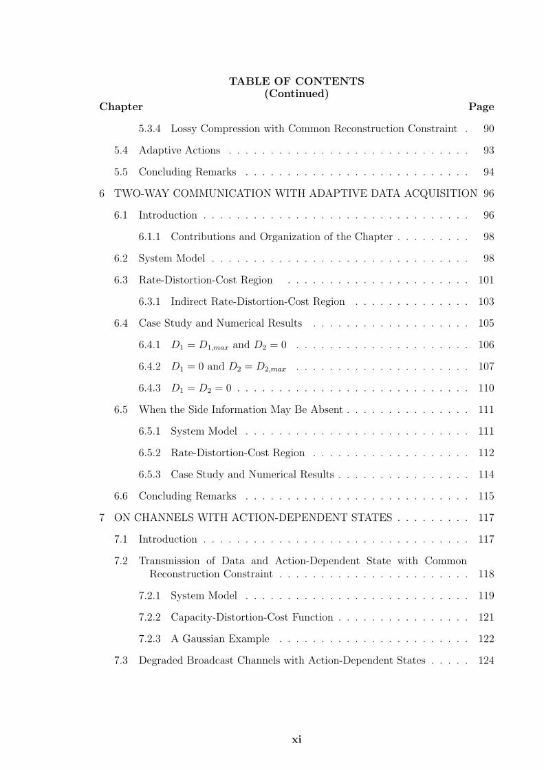
TABLE OF CONTENTS(Continued)
Chapter Page
5.3.4 Lossy Compression with Common Reconstruction Constraint . 90
5.4 Adaptive Actions . . . . . . . . . . . . . . . . . . . . . . . . . . . . . 93
5.5 Concluding Remarks . . . . . . . . . . . . . . . . . . . . . . . . . . . 94
6 TWO-WAY COMMUNICATION WITH ADAPTIVE DATA ACQUISITION 96
6.1 Introduction . . . . . . . . . . . . . . . . . . . . . . . . . . . . . . . . 96
6.1.1 Contributions and Organization of the Chapter . . . . . . . . . 98
6.2 System Model . . . . . . . . . . . . . . . . . . . . . . . . . . . . . . . 98
6.3 Rate-Distortion-Cost Region . . . . . . . . . . . . . . . . . . . . . . 101
6.3.1 Indirect Rate-Distortion-Cost Region . . . . . . . . . . . . . . 103
6.4 Case Study and Numerical Results . . . . . . . . . . . . . . . . . . . 105
6.4.1 D1 = D1,max and D2 = 0 . . . . . . . . . . . . . . . . . . . . . 106
6.4.2 D1 = 0 and D2 = D2,max . . . . . . . . . . . . . . . . . . . . . 107
6.4.3 D1 = D2 = 0 . . . . . . . . . . . . . . . . . . . . . . . . . . . . 110
6.5 When the Side Information May Be Absent . . . . . . . . . . . . . . . 111
6.5.1 System Model . . . . . . . . . . . . . . . . . . . . . . . . . . . 111
6.5.2 Rate-Distortion-Cost Region . . . . . . . . . . . . . . . . . . . 112
6.5.3 Case Study and Numerical Results . . . . . . . . . . . . . . . . 114
6.6 Concluding Remarks . . . . . . . . . . . . . . . . . . . . . . . . . . . 115
7 ON CHANNELS WITH ACTION-DEPENDENT STATES . . . . . . . . . 117
7.1 Introduction . . . . . . . . . . . . . . . . . . . . . . . . . . . . . . . . 117
7.2 Transmission of Data and Action-Dependent State with CommonReconstruction Constraint . . . . . . . . . . . . . . . . . . . . . . . 118
7.2.1 System Model . . . . . . . . . . . . . . . . . . . . . . . . . . . 119
7.2.2 Capacity-Distortion-Cost Function . . . . . . . . . . . . . . . . 121
7.2.3 A Gaussian Example . . . . . . . . . . . . . . . . . . . . . . . 122
7.3 Degraded Broadcast Channels with Action-Dependent States . . . . . 124
xi

TABLE OF CONTENTS(Continued)
Chapter Page
7.3.1 System Model . . . . . . . . . . . . . . . . . . . . . . . . . . . 125
7.3.2 Capacity-Cost Region . . . . . . . . . . . . . . . . . . . . . . . 126
7.3.3 A Binary Example . . . . . . . . . . . . . . . . . . . . . . . . . 128
7.3.4 Probing Capacity of Degraded Broadcast Channels . . . . . . . 129
7.4 Concluding Remarks . . . . . . . . . . . . . . . . . . . . . . . . . . . 131
8 INFORMATION EMBEDDING ON ACTIONS . . . . . . . . . . . . . . . 133
8.1 Introduction . . . . . . . . . . . . . . . . . . . . . . . . . . . . . . . . 133
8.1.1 Information Embedding on Actions . . . . . . . . . . . . . . . 134
8.1.2 Related Work . . . . . . . . . . . . . . . . . . . . . . . . . . . 135
8.1.3 Contributions and Chapter Organization . . . . . . . . . . . . 137
8.2 Decoder-Side Actions for Side Information Acquisition . . . . . . . . . 138
8.2.1 System Model . . . . . . . . . . . . . . . . . . . . . . . . . . . 138
8.2.2 Non-Causal Action Observation . . . . . . . . . . . . . . . . . 140
8.2.3 Strictly Causal Action Observation . . . . . . . . . . . . . . . 143
8.2.4 Causal Action Observation . . . . . . . . . . . . . . . . . . . . 146
8.2.5 Binary Example . . . . . . . . . . . . . . . . . . . . . . . . . . 148
8.3 Encoder-Side Actions for Side Information Acquisition . . . . . . . . . 151
8.4 Actions for Channel State Control and Probing . . . . . . . . . . . . 157
8.4.1 System Model . . . . . . . . . . . . . . . . . . . . . . . . . . . 157
8.4.2 Capacity-Cost Region . . . . . . . . . . . . . . . . . . . . . . . 159
8.4.3 Probing Capacity . . . . . . . . . . . . . . . . . . . . . . . . . 160
8.5 Concluding Remarks . . . . . . . . . . . . . . . . . . . . . . . . . . . 162
APPENDIX A PROOF OF PROPOSITION 3.1 . . . . . . . . . . . . . . . . 165
APPENDIX B PROOF OF PROPOSITION 3.2 . . . . . . . . . . . . . . . . 167
APPENDIX C PROOF OF (3.23) . . . . . . . . . . . . . . . . . . . . . . . . 170
APPENDIX D PROOF OF PROPOSITION 3.3 . . . . . . . . . . . . . . . . 171
xii

TABLE OF CONTENTS(Continued)
Chapter Page
APPENDIX E PROOF OF PROPOSITION 3.9 . . . . . . . . . . . . . . . . 173
APPENDIX F PROOF OF PROPOSITION 3.10 . . . . . . . . . . . . . . . 174
APPENDIX G PROOF OF PROPOSITION 3.11 . . . . . . . . . . . . . . . 175
APPENDIX H CARDINALITY BOUNDS . . . . . . . . . . . . . . . . . . . 177
APPENDIX I PROOF OF THE CONVERSE FOR PROPOSITION 4.3 . . 178
APPENDIX J PROOF OF THE CONVERSE FOR PROPOSITION 4.4 . . 180
APPENDIX K GREEDY ACTIONS ARE OPTIMAL WITH SUM SIDEINFORMATION . . . . . . . . . . . . . . . . . . . . . . . . . . . . . . . 185
APPENDIX L PROOF OF THE CONVERSE FOR PROPOSITION 4.5 . . 186
APPENDIXM CONVERSE PROOF FOR PROPOSITION 5.1 AND 5.4 . . 188
APPENDIX N PROOF OF PROPOSITION 5.3 . . . . . . . . . . . . . . . . 191
APPENDIX O CONVERSE PROOF FOR PROPOSITION 6.1 AND 6.2 . . 198
APPENDIX P PROOFS FOR THE EXAMPLE IN SECTION 6.4 . . . . . . 201
APPENDIX Q CONVERSE PROOF FOR PROPOSITION 6.3 . . . . . . . 203
APPENDIX R PROOF OF PROPOSITION 7.1 . . . . . . . . . . . . . . . . 205
APPENDIX S PROOF OF PROPOSITION 7.2 . . . . . . . . . . . . . . . . 208
APPENDIX T PROOF OF PROPOSITION 8.1 . . . . . . . . . . . . . . . . 210
APPENDIX U PROOF OF PROPOSITION 8.2 AND PROPOSITION 8.3 . 213
APPENDIX V PROOF OF PROPOSITION 8.4 . . . . . . . . . . . . . . . . 215
APPENDIXW SKETCHOF PROOFOF ACHIEVABILITY FOR PROPOSITION8.6 . . . . . . . . . . . . . . . . . . . . . . . . . . . . . . . . . . . . . . . 218
BIBLIOGRAPHY . . . . . . . . . . . . . . . . . . . . . . . . . . . . . . . . . 220
xiii

LIST OF TABLES
Table Page
6.1 Erasure Distortion for Reconstruction at Node 3. . . . . . . . . . . . . . 114
xiv

LIST OF FIGURES
Figure Page
1.1 Source coding with adaptive data acquisition. . . . . . . . . . . . . . . . 2
1.2 Source coding with adaptive data acquisition. . . . . . . . . . . . . . . . 2
1.3 Cascade source coding with adaptive data acquisition. . . . . . . . . . . 3
1.4 Channel probing. . . . . . . . . . . . . . . . . . . . . . . . . . . . . . . . 4
2.1 Source coding with side information. . . . . . . . . . . . . . . . . . . . . 11
2.2 Illustration of binning. The set of all dots represent the codebook ofcodewords Un and the subset in gray is a bin. The picture assumes forsimplicity X = U . . . . . . . . . . . . . . . . . . . . . . . . . . . . . . 12
2.3 Source coding when side information may be absent. . . . . . . . . . . . 13
2.4 Source coding with side information ”vending machine”. . . . . . . . . . 13
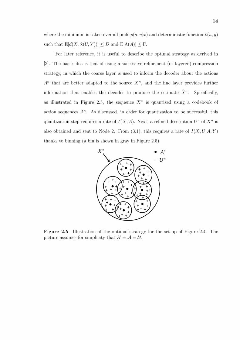
2.5 Illustration of the optimal strategy for the set-up of Figure 2.4. Thepicture assumes for simplicity that X = A = U . . . . . . . . . . . . . . 14
3.1 Point-to-point source coding with common reconstruction [8]. . . . . . . 16
3.2 Heegard-Berger source coding problem with common reconstruction. . . 17
3.3 Heegard-Berger source coding problem with common reconstruction anddecoder cooperation. . . . . . . . . . . . . . . . . . . . . . . . . . . . . 17
3.4 Cascade source coding problem with common reconstruction. . . . . . . 18
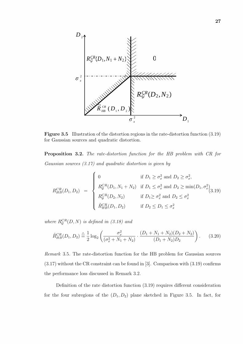
3.5 Illustration of the distortion regions in the rate-distortion function (3.19)for Gaussian sources and quadratic distortion. . . . . . . . . . . . . . 27
3.6 The rate-distortion function RCRHB(D1, D2) in (3.19) versus distortion D1
for different values of distortion D2 and for σ2x = 4, N1 = 2, and N2 = 3. 29
3.7 Illustration of the pmfs in the factorization (3.10) of the joint distributionp(x, y1, y2) for a binary source X and erased side information sequences(Y1, Y2). . . . . . . . . . . . . . . . . . . . . . . . . . . . . . . . . . . 30
3.8 Illustration of the distortion regions in the rate-distortion function (3.25)for a binary source with degraded erased side information and Hammingdistortion. . . . . . . . . . . . . . . . . . . . . . . . . . . . . . . . . . 31
3.9 Rate-distortion functions RKaspi(D1, D2) [19], RHB(D1, D2) [14] andRCR
HB(D1, D2) (3.25) for a binary source under erased side informationversus distortion D1 (p1 = 1, p2 = 0.35, D2 = 0.05 and D2 = 0.3). . . . 34
xv

LIST OF FIGURES(Continued)
Figure Page
4.1 Source coding with a vending machine at the decoder [4] with: (a) “non-causal” side information; (b) “causal” side information. . . . . . . . . 50
4.2 Distributed source coding with a side information vending machine at thedecoder. . . . . . . . . . . . . . . . . . . . . . . . . . . . . . . . . . . 51
4.3 Cascade source coding with a side information vending machine. Sideinformation is assumed to be available “causally” to the decoder. . . . 51
4.4 Sum-rates versus p for sum and product side informations (Γ = 1). . . . 63
4.5 Sum-rates versus the action cost Γ for product side information (p = 0.45). 64
4.6 Sum-rates versus the action cost Γ for sum side information (p = 0.1). . 65
5.1 A multi-hop computer network in which intermediate and end nodes canaccess side information by interrogating remote data bases via cost-constrained actions. . . . . . . . . . . . . . . . . . . . . . . . . . . . . 73
5.2 (a) Cascade source coding problem and (b) cascade-broadcast sourcecoding problem. . . . . . . . . . . . . . . . . . . . . . . . . . . . . . . 74
5.3 Cascade source coding problem with a side information “vending machine”at Node 3. . . . . . . . . . . . . . . . . . . . . . . . . . . . . . . . . . 76
5.4 Cascade source coding problem with a side information “vending machine”at Node 2 and Node 3. . . . . . . . . . . . . . . . . . . . . . . . . . . 77
5.5 Cascade-broadcast source coding problem with a side information “vendingmachine” at Node 2. . . . . . . . . . . . . . . . . . . . . . . . . . . . . 78
5.6 The side information S-channel p(w|x) used in the example of Section 5.3.3. 88
5.7 Difference between the weighted sum-rate R1 + ηR2 obtained with thegreedy and with the optimal strategy as per Corollary 5.2 (Rb = 0.4,δ = 0.6). . . . . . . . . . . . . . . . . . . . . . . . . . . . . . . . . . . 89
6.1 Two-way communication with adaptive data acquisition. . . . . . . . . . 97
6.2 Two-way source coding with a side information vending machine at Node 2. 98
6.3 Indirect two-way source coding with a side information vending machineat Node 2. . . . . . . . . . . . . . . . . . . . . . . . . . . . . . . . . . 104
6.4 Rate R1 versus cost Γ for the examples in Section 6.4 with ϵ = 0.2. . . . 109
6.5 Indirect two-way source coding when the side information vendingmachine may be absent at the recipient of the message from Node 1. . 112
xvi

LIST OF FIGURES(Continued)
Figure Page
6.6 Rate R1 versus cost Γ for the examples in Section 6.5.3 with ϵ = 0.2,D1 = 0 and D2 = D2,max. . . . . . . . . . . . . . . . . . . . . . . . . . 116
7.1 Channel with action-dependent state in which the decoder estimatesboth message and state, and there is a a common reconstruction (CR)constraint on the state reconstruction. The state is known non-causallyat the channel encoder. . . . . . . . . . . . . . . . . . . . . . . . . . . 118
7.2 Broadcast channel with action-dependent states known causally to theencoder (i.e., the ith transmitted symbol Xi is a function of messagesM1, M2 and the state symbols up to time i, Si). . . . . . . . . . . . . 119
7.3 Achievable rates (constrained to a Gaussian joint distribution, see (7.16))for the Gaussian model (7.14)-(7.15) versus distortion D for PA = PX =σ2W = σ2
Z = 1. . . . . . . . . . . . . . . . . . . . . . . . . . . . . . . . 124
8.1 Source coding with decoder-side actions for information acquisition andwith information embedding on actions. A function of the actionsf(An) = (f(A1), ..., f(An)) is observed in full (“non-causally”) by Decoder2 before decoding. See Figure 8.4 and Figure 8.5 for the correspondingmodels with strictly causal and causal observation of the actions atDecoder 2, respectively. . . . . . . . . . . . . . . . . . . . . . . . . . . 135
8.2 Source coding with encoder-side actions for information acquisition andwith information embedding on actions. . . . . . . . . . . . . . . . . . 136
8.3 Channel coding with actions for channel state control and with infor-mation embedding on actions. . . . . . . . . . . . . . . . . . . . . . . 136
8.4 Source coding with decoder-side actions for information acquisition andwith information embedding on actions. At time i, Decoder 2 hasavailable the samples f(Ai−1) = (f(A1), ..., f(Ai−1)) in a strictly causalfashion. . . . . . . . . . . . . . . . . . . . . . . . . . . . . . . . . . . . 144
8.5 Source coding with decoder-side actions for information acquisition andwith information embedding on actions. At time i, Decoder 2 hasavailable the samples f(Ai) = (f(A1), ..., f(Ai)) in a causal fashion. . . . 146
8.6 The side information channel p(y|x, a) used in the example of Section 8.2.5.149
8.7 Rate-distortion function R(0, D2, 1) in (8.18) versus distortion D2 withthe side information channel in Figure 8.6 (non-causal side information).150
8.8 Difference between the rate-distortion function (8.18) with non-causal(NC) and strictly causal (SC) action observation versus δ for valuesof distortion D2 = 0.1, 0.2 and 0.3. . . . . . . . . . . . . . . . . . . . . 150
xvii

LIST OF FIGURES(Continued)
Figure Page
8.9 Channel coding with actions for channel state probing and with infor-mation embedding on actions. . . . . . . . . . . . . . . . . . . . . . . 160
8.10 Sum-rate R1+R2 versus the input cost constraint ΓX for values of R1 = 0,R1 = 0.5 and R1 = 0.9. . . . . . . . . . . . . . . . . . . . . . . . . . . 163
J.1 Bayesian network representing the joint pmf of variables (M1, Xn1 , X
n2 , A
n, Y n)for the model in Figure 4.2. . . . . . . . . . . . . . . . . . . . . . . . . 184
O.1 Bayesian network representing the joint pmf of variables (M1,M2, Xn, Y n, An)
for the two-way source coding problem with a vending machine in Figure6.2. . . . . . . . . . . . . . . . . . . . . . . . . . . . . . . . . . . . . . 199
W.1 Illustration of the rate regions (8.39) (dashed lines) and (W.1) (solid lines).218
xviii

CHAPTER 1
MOTIVATION AND OVERVIEW
In communication systems such as data networks, sensor networks and local area
networks, sensitive data is transferred through multiple hops. Examples are financial,
military and medical. This data often needs to be acquired from the “environment”,
such as from databases or via sensor measurements. Beside data acquisition, nodes
also need to take various type of actions, e.g., to probe the state of the network prior
to transmission.
The aim of this thesis is to address two important questions that arise in the
design of the outlined communication networks: 1) How to preserve the consistency
of sensitive information to be sent over multi-hop networks? 2) How to integrate the
optimization of actuation tasks, such as for data acquisition or network probing, in the
design of communication networks? These issues are addressed from an information-
theoretic point of view. To this end, several source and channel coding systems are
investigated that exemplify various key scenarios of interest.
To address the first issue, one has to guarantee that downstream nodes use the
locally available information in such as way that no inconsistency is created with the
state of knowledge of upstream nodes. This requirement is known in information
theory as the Common Reconstruction (CR) constraint. Under this constraint, this
thesis derives the rate-distortion performance for the so called Heegard-Berger (HB)
problem and for the cascade source coding problem.
The second aforementioned issue is tackled by focusing on two specific actuation
tasks, namely adaptive data acquisition and channel probing. Adaptive data
acquisition addresses the problem of using efficiently the system resources in order
to acquire information to the environment. Applications include sensor networks,
1
2
Enc Dec 1
Data base server
information
side information Adaptive
data acquisiton
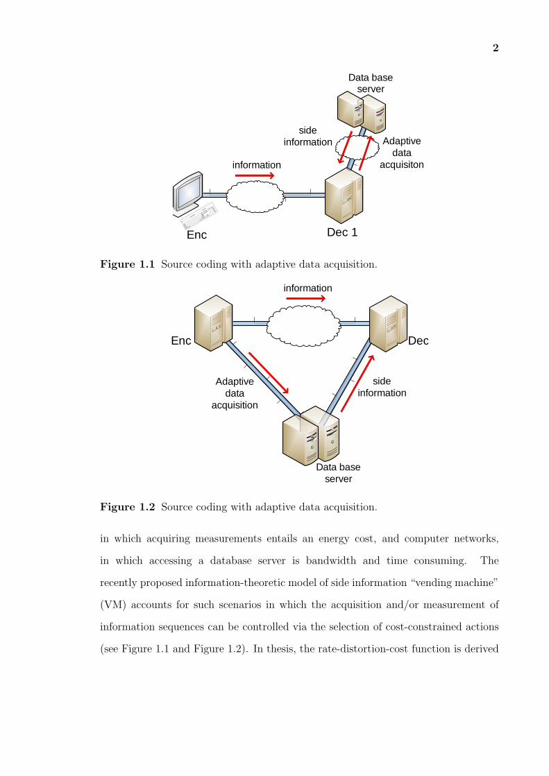
Figure 1.1 Source coding with adaptive data acquisition.
Enc Dec 1
information
side information
Data base server
Adaptive data
acquisition
Figure 1.2 Source coding with adaptive data acquisition.
in which acquiring measurements entails an energy cost, and computer networks,
in which accessing a database server is bandwidth and time consuming. The
recently proposed information-theoretic model of side information “vending machine”
(VM) accounts for such scenarios in which the acquisition and/or measurement of
information sequences can be controlled via the selection of cost-constrained actions
(see Figure 1.1 and Figure 1.2). In thesis, the rate-distortion-cost function is derived
3
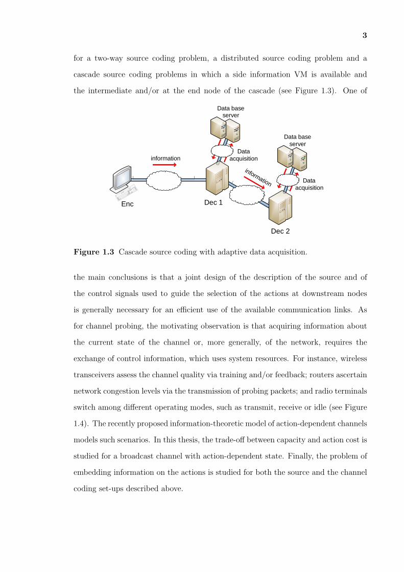
for a two-way source coding problem, a distributed source coding problem and a
cascade source coding problems in which a side information VM is available and
the intermediate and/or at the end node of the cascade (see Figure 1.3). One of
Enc Dec 1
Data base server
information
Dec 2
Data base server
Data acquisition
Data acquisition
information
Figure 1.3 Cascade source coding with adaptive data acquisition.
the main conclusions is that a joint design of the description of the source and of
the control signals used to guide the selection of the actions at downstream nodes
is generally necessary for an efficient use of the available communication links. As
for channel probing, the motivating observation is that acquiring information about
the current state of the channel or, more generally, of the network, requires the
exchange of control information, which uses system resources. For instance, wireless
transceivers assess the channel quality via training and/or feedback; routers ascertain
network congestion levels via the transmission of probing packets; and radio terminals
switch among different operating modes, such as transmit, receive or idle (see Figure
1.4). The recently proposed information-theoretic model of action-dependent channels
models such scenarios. In this thesis, the trade-off between capacity and action cost is
studied for a broadcast channel with action-dependent state. Finally, the problem of
embedding information on the actions is studied for both the source and the channel
coding set-ups described above.

4
Enc Dec
Probing
Channel State
Figure 1.4 Channel probing.
1.1 Organization and Contributions
In this section, the main contributions and organization of the thesis are outlined.
Chapter 2: A very short introduction of the fundamental information theoretic
concepts is provided in this Chapter.
Chapter 3: This Chapter investigates the problems Heegard-Berger(HB) and
cascade source coding with common reconstruction constraint. The HB problem
consists of an encoder broadcasting to two decoders with respective side information.
The cascade source coding problem is characterized by a two-hop system with side
information available at the intermediate and nal nodes. For the HB problem with the
CR constraint, the rate-distortion function is derived under the assumption that the
side information sequences are (stochastically) degraded. The rate-distortion function
is also calculated explicitly for three examples, namely Gaussian source and side
information with quadratic distortion metric, and binary source and side information
with erasure and Hamming distortion metrics. The rate-distortion function is
then characterized for the HB problem with cooperating decoders and (physically)
degraded side information. For the cascade problem with the CR constraint, the
rate-distortion region is obtained under the assumption that side information at the
nal node is physically degraded with respect to that at the intermediate node. For the
latter two cases, it is worth emphasizing that the corresponding problem without the

5
CR constraint is still open. Outer and inner bounds on the rate-distortion region are
also obtained for the cascade problem under the assumption that the side information
at the intermediate node is physically degraded with respect to that at the nal node.
For the three examples mentioned above, the bounds are shown to coincide. Finally,
for the HB problem, the rate-distortion function is obtained under the more general
requirement of constrained reconstruction, whereby the decoders estimate must be
recovered at the encoder only within some distortion.
The material in this chapter has been reported in the documents:
• B. Ahmadi, R. Tandon, O. Simeone and H. V. Poor, “Heegard-Berger and
Cascade Source Coding Problems with Common Reconstruction Constraints,”
IEEE Trans. Inform. Theory, vol. 59, no. 3, pp. 1458,1474, Mar. 2013.
• B. Ahmadi, R. Tandon, O. Simeone and H. V. Poor, “On the Heegard-
Berger Problem with Common Reconstruction Constraints,” in Proc. IEEE
International Symposium on Information Theory (ISIT 2012), Cambridge, MA,
USA, July 1-6, 2012.
Chapter 4: In this Chapter, the analysis of the trade-offs between rate,
distortion and cost associated with the control actions is extended from the previously
studied point-to-point set-up to two basic multiterminal models. First, a distributed
source coding model is studied, in which two encoders communicate over rate-limited
links to a decoder, whose side information can be controlled. The control actions
are selected by the decoder based on the messages encoded by both source nodes.
For this set-up, inner bounds are derived on the rate-distortion-cost region for both
cases in which the side information is available causally and non-causally at the
decoder. These bounds are shown to be tight under specic assumptions, including
the scenario in which the sequence observed by one of the nodes is a function of the
source observed by the other and the side information is available causally at the

6
decoder. Then, a cascade scenario in which three nodes are connected in a cascade
and the last node has controllable side information, is also investigated. For this
model, the rate-distortion-cost region is derived for general distortion requirements
and under the assumption of causal availability of side information at the last node.
The material in this chapter has been reported in the documents:
• B. Ahmadi and O. Simeone, “Distributed and Cascade Lossy Source Coding
with a Side Information “Vending Machine”,” to appear in IEEE Trans. Inform.
Theory, arXiv:1109.6665.
• B. Ahmadi and O. Simeone, “Distributed and Cascade Lossy Source Coding
with a Side Information “Vending Machine”,” in Proc. IEEE International
Symposium on Information Theory (ISIT 2012), Cambridge, MA, USA, July
1-6, 2012.
Chapter 5:: In this Chapter, a three-node cascade source coding problem
is studied under the assumption that a side information VM is available and the
intermediate and/or at the end node of the cascade. A single-letter characterization
of the achievable trade-off among the transmission rates, the distortions in the
reconstructions at the intermediate and at the end node, and the cost for acquiring
the side information is derived for a number of relevant special cases. It is shown
that a joint design of the description of the source and of the control signals used to
guide the selection of the actions at downstream nodes is generally necessary for an
efcient use of the available communication links. In particular, for all the considered
models, layered coding strategies prove to be optimal, whereby the base layer fullls two
network objectives: determining the actions of downstream nodes and simultaneously
providing a coarse description of the source. Design of the optimal coding strategy
is shown via examples to depend on both the network topology and the action costs.
Examples also illustrate the involved performance trade-offs across the network.

7
The material in this chapter has been reported in the documents:
• B. Ahmadi, C. Choudhuri, O. Simeone and U. Mitra, “Cascade source coding
with a side information “vending machine”,” submitted to IEEE Trans. Inform.
Theory, arXiv:1207.2793.
• B. Ahmadi, O. Simeone, C. Choudhuri and U. Mitra, “On Cascade Source
Coding with A Side Information “Vending Machine”,” in Proc. IEEE
Information Theory Workshop (ITW 2012), Lausanne, Switzerland, Sept. 3-7,
2012.
Chapter 6: In this Chapter, a bidirectional link is studied in which two
nodes, Node 1 and Node 2, communicate to fulfill generally conflicting informational
requirements. Node 2 is able to acquire information from the environment, e.g., via
access to a remote database or via sensing. Information acquisition is expensive in
terms of system resources, e.g., time, bandwidth and energy, and thus should be done
efficiently by adapting the acquisition process to the needs of the application. As
a result of the forward communication from Node 1 to Node 2, the latter wishes
to compute some function, such as a suitable average, of the data available at
Node 1 and of the data obtained from the environment. The forward link is also
used by Node 1 to query Node 2 with the aim of retrieving suitable information
from the environment on the backward link. The problem is formulated in the
context of multi-terminal rate-distortion theory and the optimal trade-off between
communication rates, distortions of the information produced at the two nodes and
costs for information acquisition at Node 2 is derived. The issue of robustness to
possible malfunctioning of the data acquisition process at Node 2 is also investigated.
The results are illustrated via an example that demonstrates the different roles played
by the forward communication, namely data exchange, query and control.
The material in this chapter has been reported in the documents:

8
• B. Ahmadi and O. Simeone, “Two-way Communication with Adaptive Data
Acquisition,” to appear in Transactions on Emerging Telecommunications
Technologies, arXiv:1209.5978.
• B. Ahmadi and O. Simeone, “Two-Way Communication with Adaptive Data
Acquisition,” in Proc. IEEE International Symposium on Information Theory
(ISIT 2013), Istanbul, Turkey, July 7-12, 2013.
Chapter 7: In this Chapter, two extensions of the original action-dependent
channel are studied. In the first, the decoder is interested in estimating not only
the message, but also the state sequence within an average per-letter distortion.
Under the constraint of common reconstruction (i.e., the decoders estimate of the
state must be recoverable also at the encoder) and assuming non-causal state
knowledge at the encoder in the second phase, a single-letter characterization of
the achievable rate-distortion-cost trade-off is obtained. In the second extension, an
action-dependent degraded broadcast channel is studied. Under the assumption that
the encoder knows the state sequence causally in the second phase, the capacity-cost
region is identified. Various examples, including Gaussian channels and a model with
a ”probing” encoder, are also provided to show the advantage of a proper joint design
of the two communication phases.
The material in this chapter has been reported in the documents:
• B. Ahmadi and O. Simeone, “On Channels with Action-Dependent States,” in
Proc. IEEE Information Theory Workshop (ITW 2012), Lausanne, Switzerland,
Sept. 3-7, 2012.
• B. Ahmadi and O. Simeone, “On channels with action-dependent states,”
arXiv:1202.4438.
Chapter 8: In this Chapter, the problem of embedding information on the
actions is studied for both the source and the channel coding set-ups. In both

9
cases, a decoder is present that observes only a function of the actions taken by
an encoder or a decoder of an action-dependent point-to-point link. For the source
coding model, this decoder wishes to reconstruct a lossy version of the source being
transmitted over the point-to-point link, while for the channel coding problem the
decoder wishes to retrieve a portion of the message conveyed over the link. For
the problem of source coding with actions taken at the decoder, a single letter
characterization of the set of all achievable tuples of rate, distortions at the two
decoders and action cost is derived, under the assumption that the mentioned decoder
observes a function of the actions non-causally, strictly causally or causally. A special
case of the problem in which the actions are taken by the encoder is also solved. A
single-letter characterization of the achievable capacity-cost region is then obtained
for the channel coding set-up with actions. Examples are provided that shed light into
the effect of information embedding on the actions for the action-dependent source
and channel coding problems.
The material in this chapter has been reported in the documents:
• B. Ahmadi, H. Asnani, O. Simeone and H. Permuter, “Information Embedding
on Actions,” in Proc. IEEE International Symposium on Information Theory
(ISIT 2013), Istanbul, Turkey, July 7-12, 2013.
• B. Ahmadi, H. Asnani, O. Simeone and H. Permuter, “Information Embedding
on Actions,” submitted to IEEE Trans. Inform. Theory, arXiv:1207.6084.

CHAPTER 2
PRELIMINARIES
In this chapter, first the notation used is discussed and then, some preliminary
information-theoretic results on related problems in the field of source coding with
side information are studied.
2.1 Notation
For a and b integer with a ≤ b, [a, b] is defined as the interval [a, a+1, ..., b] and xba is
used to denote the sequence (xa, . . . , xb). Also xb is written for xb1 for simplicity. Upper
case, lower case and calligraphic letters denote random variables, specific values of
random variables and their alphabets, respectively. Given discrete random variables,
or more generally vectors, X and Y , the notation pX(x) or p(x) is used for Pr[X = x],
and pX|Y (x|y) or p(x|y) is used for Pr[X = x|Y = y], where the latter notations
are used when the meaning is clear from the context. Given a set X , an n-fold
Cartesian product of X is denoted by X n. For random variables X and Y , σ2X|Y is the
(average) conditional variance of X given Y , i.e., E [E[(X − E[X|Y ])2|Y ]] . Function
δ(x) represents the Kronecker delta function, i.e., δ(x) = 1 if x = 0 and δ(x) = 0
otherwise. The notation convention in [1] is adopted, in which δ(ϵ) represents any
function such that δ(ϵ) → 0 as ϵ → 0. Moreover, X—Y—Z form a Markov chain if
p(x, y, z) = p(x)p(y|x)p(z|y), that is, X and Z are conditionally independent of each
other given Y . The binary entropy function is defined as H(p) = −plog2p − (1 −
p)log2(1− p). Finally, α ∗ β = α(1− β) + β(1− α).
2.2 Background
From an information theoretic perspective, the baseline setting for the class of source
coding problems with side information is one in which a memoryless source Xn =
10

11
(X1, ..., Xn), where Xi ∈ X has pmf p(x) for i = 1, ..., n, is to be communicated by an
encoder via a message M of rate R bits per source symbol to a decoder. The decoder
has available a correlated sequence Y n, with Yi ∈ Y , that is related to Xn via a
memoryless channel p(y|x) (see Figure 2.1). The optimal trade-off between rate R and
the average distortion D between the source Xn and reconstruction Xn was obtained
by Wyner and Ziv in [2] for any given distortion metric d(x, x) : X ×X → R+∪{∞}.
It was shown that the rate-distortion function is given by
R(D) = min I(X;U |Y ), (2.1)
where the minimum is taken over all pmfs p(u|x), with u ∈ U , and deterministic
function x(u, y) such that E[d(X, x(U, Y ))] ≤ D.
The optimal performance can be achieved as follows. The sequence Xn is
quantized using a randomly generated codebook of codewords Un using the standard
joint typicality criterion. In order for quantization to be successful 2nI(X;U) codewords
Un are sufficient. Thanks to the side information Y n available at Node 2, the resulting
rate I(X;U) (bits per source symbol) can be further decreased to I(X;U |Y ) using
the technique of binning. The idea is that all the 2nI(X;U) codewords Un are divided
into 2nI(X;U |Y ) bins. An example of a bin is shown in gray in Figure 2.2. The
codewords Un in the same bin are mapped to an identical message M . The bins
contain 2nI(X;U)/2nI(X;U |Y ) = 2nI(U ;Y ) codewords each, and thus, by the channel coding
theorem, the decoder can distinguish among the codewords Un in the bin based on
Y n. This scheme is known as ”Wyner-Ziv” coding in information theory.
Node 1nX
nY
MNode 2 nX
nX ( | )p y x
Figure 2.1 Source coding with side information.

12
nX
Figure 2.2 Illustration of binning. The set of all dots represent the codebook ofcodewords Un and the subset in gray is a bin. The picture assumes for simplicityX = U .
In sensor networks and cloud computing, reliability of all the computing devices
(e.g., sensors or servers) cannot be guaranteed all the time. Therefore, it is appropriate
to design the system so as to be robust to system failures. As shown in Figure 2.3, this
aspect can be modeled by assuming that the decoder, unbeknownst to the encoder,
may not be able to acquire information sequence Y n. This setting is equivalent to
assuming the presence of two decoders, one with the capability to acquire information
about Y n (Node 2) and one without this capability (Node 3). This model is referred to
as the Heegard-Berger problem, where Node 2 and Node 3 of Figure 2.3 are interested
in estimating Xn2 and Xn
3 , respectively. It is emphasized that Xn2 and Xn
3 are two
different description of the source sequence Xn to be reconstructed at Node 2 and
Node 3 with distortion levels D2 and D3, respectively.
It was shown in [3] that the rate-distortion function is given by
R(D2, D3) = min I(X; X3) + I(X;U |X3, Y ), (2.2)
where the minimum is taken over all pmfs p(u, x3|x) and deterministic function
x2(u, y) such that E[d(X, X3))] ≤ D3 and E[d(X, x2(U, Y ))] ≤ D2. The optimal
strategy achieving (2.2) is based on successive refinement and binning. The strategy
is identical to that used below in the context of the model of Figure 2.4 (see Figure
2.5 and discussion below for further details).

13
Node 1n
X
nY
MNode 2
nX2
ˆ
Node 3n
X3
ˆ
Figure 2.3 Source coding when side information may be absent.
The concept of a side information “vending machine” was introduced in [4] in
order to account for source coding scenarios in which acquiring the side information
at the receiver entails some cost and thus should be done efficiently. In this
class of models, the quality of the side information Y n can be controlled at the
decoder by selecting an action sequence An, with Ai ∈ A, that affects the effective
channel between the source Xn and the side information Y n through a conditional
memoryless distribution pY |X,A(y|x, a). Specifically, given An and Xn, the sequence
Y n is distributed as p(yn|an, xn) =∏n
i=1 pY |A,X(yi|ai, xi). The cost of the action
sequence is defined by a cost function Λ: A →[0,Λmax] with 0 ≤ Λmax < ∞, as
Λ(an) =∑n
i=1 Λ(ai). The estimated sequence Xn with Xn ∈ X n is then obtained as
a function of M and Y n.
Node 1
nA
ˆ nX
( | , )p y a x
Node 2M
nX
nY
nX
Figure 2.4 Source coding with side information ”vending machine”.
The optimal trade-off between rate R, the average distortion D and the average
action cost Γ was obtained by [4] for any given distortion metric d(x, x) and action
cost function Λ(a) is given by
R(D,Γ) = min I(X;A) + I(X;U |Y,A), (2.3)
14
where the minimum is taken over all pmfs p(a, u|x) and deterministic function x(u, y)
such that E[d(X, x(U, Y ))] ≤ D and E[Λ(A)] ≤ Γ.
For later reference, it is useful to describe the optimal strategy as derived in
[3]. The basic idea is that of using a successive refinement (or layered) compression
strategy, in which the coarse layer is used to inform the decoder about the actions
An that are better adapted to the source Xn, and the fine layer provides further
information that enables the decoder to produce the estimate Xn. Specifically,
as illustrated in Figure 2.5, the sequence Xn is quantized using a codebook of
action sequences An. As discussed, in order for quantization to be successful, this
quantization step requires a rate of I(X;A). Next, a refined description Un of Xn is
also obtained and sent to Node 2. From (3.1), this requires a rate of I(X;U |A, Y )
thanks to binning (a bin is shown in gray in Figure 2.5).
nX nAnU
�
�
�
��
��
�
�
�
� �
�
�
�
�
�
�
�
�
�
�
�
�
�
�
��
�
�
�
�
�
��
���
�
�
�
�
�
��
�
�
�
�
�
�
�
�
��
�
�
�
�
��
��
�
�
�
�
�
�
�
�
�
Figure 2.5 Illustration of the optimal strategy for the set-up of Figure 2.4. Thepicture assumes for simplicity that X = A = U .

CHAPTER 3
HEEGARD-BERGER AND CASCADE SOURCE CODING WITH
COMMON RECONSTRUCTION CONSTRAINT
3.1 Introduction
Source coding problems with side information at the decoder(s) model a large number
of scenarios of practical interest, including video streaming [5] and wireless sensor
networks [6]. From an information theoretic perspective, the baseline setting for
this class of problems is one in which a memoryless source Xn = (X1, ..., Xn) is to
be communicated by an encoder at a rate R bits per source symbol to a decoder
that has available a correlated sequence Y n that is related to Xn via a memoryless
channel p(y|x) (see Figure 3.11). Under the requirement of asymptotically lossless
reconstruction Xn of the source Xn at the decoder, the minimum required rate was
obtained by Slepian andWolf in [7]. Later, the more general optimal trade-off between
rate R and the distortion D between the source Xn and reconstruction Xn was
obtained by Wyner and Ziv in [2] for any given distortion metric d(x, x). As shown
in Chapter 2, the rate-distortion function is given by
RWZX|Y (D) = min I(X;U |Y ), (3.1)
where the minimum is taken over all probability mass functions (pmfs) p(u|x) and
deterministic function x(u, y) such that E[d(X, x(U, Y ))] ≤ D.
3.1.1 Heegard-Berger and Cascade Source Coding Problems
In applications such as the ones discussed above, the point-to-point setting of Figure
3.1 does not fully capture the main features of the source coding problem. For
1The presence of the function ψ at the encoder will be explained later.
15

16
EncodernX
ψnY
RDecoder nX
)( nXψ
Figure 3.1 Point-to-point source coding with common reconstruction [8].
instance, in video streaming, a transmitter typically broadcasts information to a
number of decoders. As another example, in sensor networks, data is typically routed
over multiple hops towards the destination. A model that accounts for the aspect
of broadcasting to multiple decoders is the Heegard-Berger (HB) set-up shown in
Figure 3.2. In this model, the link of rate R bits per source symbol is used to
communicate to two receivers having different side information sequences, Y n1 and Y n
2 ,
which are related to source Xn via a memoryless channel p(y1, y2|x). The set of all
achievable triples (R,D1, D2) for this model, whereD1 andD2 are the distortion levels
at Decoders 1 and 2, respectively was derived in [3] and [9] under the assumption that
the side information sequences are (stochastically) degraded versions of the sourceXn.
In a variation of this model shown in Figure 3.3, decoder cooperation is enabled by a
limited capacity link from one decoder (Decoder 1) to the other (Decoder 2). Inner
and outer bounds to the rate distortion region for this problem are obtained in [10]
under the assumption that the side information of Decoder 2 is (physically) degraded
with respect to that of Decoder 1.
As for multihopping, a basic model that captures some of the key design issues
is shown in Figure 3.4. In this cascade set-up, an encoder (Node 1) communicates
with rate R1 to a intermediate node (Node 2), which has side information Y n1 , and in
turns communicates with rate R2 to a final node (Node 3) with side information Y n2 .
Both Node 2 and Node 3 act as decoders, similar to the HB problem of Figure 3.2, in
the sense that they reconstruct a local estimate of the source Xn. The rate-distortion

17
EncodernX
1ψ
nY2
R
Decoder 2nX 2
ˆ
)(1nXψ
nY1
Decoder 1nX1
ˆ
2ψ
)(2nXψ
Figure 3.2 Heegard-Berger source coding problem with common reconstruction.
EncodernX
1ψ
nY2
1R
Decoder 2nX 2
ˆ
)(1nXψ
nY1
Decoder 1nX1
ˆ
2ψ
)(2nXψ
2R
Figure 3.3 Heegard-Berger source coding problem with common reconstruction anddecoder cooperation.
function for this problem has been derived for various special cases in [11, 12, 13] and
[14] (see Table I in [14] for an overview). Reference [13] derives the set of all achievable
quadruples (R1, R2, D1, D2), i.e., the rate-distortion region, for the case in which Y n1
is also available at the encoder and Y n2 is a physically degraded version of Xn with
respect to Y n1 . Instead, [12] derives the rate-distortion region under the assumptions
that the source and the side information sequences are jointly Gaussian, that the
distortion metric is quadratic, and that the sequence Y n1 is a physically degraded
version of Xn with respect to Y n2 . The corresponding result for binary source and
side information and Hamming distortion metric was derived in [14].

18
Node 2Node 1nX 1R nX 2ˆNode 32R
nX1ˆ
1ψ
)(1nXψ
nY12ψ
)(2nXψ
nY2
Figure 3.4 Cascade source coding problem with common reconstruction.
3.1.2 Common Reconstruction Constraint
A key aspect of the optimal strategies identified in [2, 3, 9, 12] and [13] is that
the side information sequences are, in general, used in two different ways: (i) as a
means to reduce the rate required for communication between encoder and decoders
via binning; and (ii) as an additional observation that the decoder can leverage,
along with the bits received from the encoder, in order to improve its local estimate.
For instance, for the point-to-point system of Figure 3.1, the Wyner-Ziv result (3.1)
reflects point (i) of the discussion above in the conditioning on side information Y ,
which reduces the rate, and point (ii) in the fact that the reconstruction X is a
function x(U, Y ) of the signal U received from the encoder and the side information
Y .
Leveraging the side information as per point (ii), while advantageous in terms of
rate-distortion trade-off, may have unacceptable consequences for some applications.
In fact, this use of side information entails that the reconstruction X of the decoder
cannot be reproduced at the encoder. In other words, encoder and decoder cannot
agree on the specific reconstruction X obtained at the receiver side, but only on the
average distortion level D. In applications such as transmission of sensitive medical,
military or financial data, this may not be desirable. Instead, one may want to add
the constraint that the reconstruction at the decoder be reproducible by the encoder
[8]. This idea, referred to as the Common Reconstruction (CR) constraint, was first

19
proposed in [8], where it is shown for the point-to-point setting of Figure 3.12 that
the rate-distortion function under the CR constraint is given by
RCRX|Y (D) = min I(X; X|Y ), (3.2)
where the minimum is taken over all pmfs p(x|x) such that E[d(X, X)] ≤ D.
Comparing (3.2) with the Wyner-Ziv rate-distortion (3.1), it can be seen that the
additional CR constraint prevents the decoder from using the side information as a
means to improve its estimate X (see point (ii) above).
The original work of [8] has been recently extended in [15], where a relaxed CR
constraint is imposed in which only a distortion constraint is imposed between the
decoder’s reconstruction and its reproduction at the encoder. This setting is referred
to as imposing a Constrained Reconstruction (ConR) requirement.
3.1.3 Main Contributions
In this Chapter, the HB source coding problem (Figure 3.2) and the cascade source
coding problem (Figure 3.4) are studied under the CR requirement. The considered
models are thus relevant for the transmission of sensitive information, which is
constrained by CR, via broadcast or multi-hop links – a common occurrence in, e.g.,
medical, military or financial applications (e.g., for intranets of hospitals or financial
institutions). Specifically, our main contributions are:
• For the HB problem with the CR constraint (Figure 3.2), the rate-distortion
function is derived under the assumption that the side information sequences
are (stochastically) degraded. Also this function is calculated explicitly for
three examples, namely Gaussian source and side information with quadratic
distortion metric, and binary source and erasure side information with erasure
and Hamming distortion metrics (Section 3.2);
2The function ψ at the encoder calculates the estimate of the encoder regarding the decoder’sreconstruction.

20
• For the HB problem with the CR constraint and decoder cooperation (Figure
3.3), the rate-distortion region is derived under the assumption that the side
information sequences are (physically) degraded in either direction (Section
3.3.1 and Section 3.3.2). It is emphasized that the corresponding problem
without the CR constraint is still open as per the discussion above;
• For the cascade problem with the CR constraint (Figure 3.4), the rate-distortion
region is obtained under the assumption that side information Y2 is physically
degraded with respect to Y1 (Section 3.4.2). It is emphasized that the
corresponding problem without the CR constraint is still open as per the
discussion above;
• For the cascade problem with CR constraint (Figure 3.4), outer and inner
bounds on the rate-distortion region are obtained under the assumption that
the side information Y1 is physically degraded with respect to Y2. Moreover,
for the three examples mentioned above in the context of the HB problem, it is
shown that the bounds coincide and the corresponding rate-distortion region is
explicitly evaluated (Section 3.4.3);
• For the HB problem, the rate-distortion function is finally derived under the
more general requirement of ConR (Section 3.5).
3.2 Heegard-Berger Problem with Common Reconstruction
In this section, first the system model for the HB source coding problem in Figure 3.2
with CR is detailed in Section 3.2.1. Next, the characterization of the corresponding
rate-distortion performance is derived under the assumption that one of the two
side information sequences is a stochastically degraded version of the other in the
sense of [3] (see (3.10)). Finally, three specific examples are worked out, namely
Gaussian sources under quadratic distortion (Section 3.2.3), and binary sources with

21
side information sequences subject to erasures under Hamming or erasure distortion
(Section 3.2.4).
3.2.1 System Model
In this section, the system model for the HB problem with CR is detailed. The system
is defined by the pmf pXY1Y2(x, y1, y2) and discrete alphabets X ,Y1,Y2, X1, and X2 as
follows. The source sequence Xn and side information sequences Y n1 and Y n
2 , with
Xn ∈ X n, Y n1 ∈ Yn
1 , and Yn2 ∈ Yn
2 are such that the tuples (Xi, Y1i, Y2i) for i ∈ [1, n]
are independent and identically distributed (i.i.d.) with joint pmf pXY1Y2(x, y1, y2).
The encoder measures a sequence Xn and encodes it into a message J of nR bits,
which is delivered to the decoders. Decoders 1 and 2 wish to reconstruct the source
sequence Xn within given distortion requirements, to be discussed below, as Xn1 ∈ X n
1
and Xn2 ∈ X n
2 , respectively. The estimated sequence Xnj is obtained as a function of
the message J and the side information sequence Y nj for j = 1, 2. The estimates are
constrained to satisfy distortion constraints defined by per-symbol distortion metrics
dj(x, xj) : X × Xj → [0, Dmax] with 0 < Dmax < ∞. Based on the given distortion
metrics, the overall distortion for the estimated sequences xn1 and xn2 is defined as
dnj (xn, xnj ) =
1
n
n∑i=1
dj(xi, xji) for j = 1, 2. (3.3)
The reconstructions Xn2 and Xn
2 are also required to satisfy the CR constraints, as
formalized below.
Definition 3.1. An (n,R,D1, D2, ϵ) code for the HB problem with CR consists of
an encoding function
g: X n → [1, 2nR], (3.4)

22
which maps the source sequenceXn into a message J ; a decoding function for Decoder
1,
h1: [1, 2nR]× Yn
1 → X n1 , (3.5)
which maps the message J and the side information Y n1 into the estimated sequence
Xn1 ; a decoding function for Decoder 2
h2: [1, 2nR]× Yn
2 → X n2 (3.6)
which maps message J and the side information Y n2 into the estimated sequence Xn
2 ;
and two reconstruction functions
ψ1: X n → X n1 (3.7a)
and ψ2: X n → X n2 , (3.7b)
which map the source sequence into the estimated sequences at the encoder, namely
ψ1(Xn) and ψ2(X
n), respectively; such that the distortion constraints are satisfied,
i.e.,
1
n
n∑i=1
E[dj(Xi, Xji)
]≤ Dj for j = 1, 2, (3.8)
and the CR requirements hold, namely,
Pr[ψj(X
n) = Xnj
]≤ ϵ, j = 1, 2. (3.9)
Given distortion pairs (D1, D2), a rate pair R is said to be achievable if, for any
ϵ > 0 and sufficiently large n, there exists an (n,R,D1 + ϵ,D2 + ϵ, ϵ) code. The rate-
distortion function R(D1, D2) is defined as R(D1, D2) =inf{R : the triple (R,D1, D2)
is achievable}.

23
3.2.2 Rate-Distortion Function
In this section, a single-letter characterization of the rate-distortion function for the
HB problem with CR is derived, under the assumption that the joint pmf p(x, y1, y2)
is such that there exists a conditional pmf p(y1|y2) for which
p(x, y1) =∑y2∈Y2
p(x, y2)p(y1|y2). (3.10)
In other words, the side information Y1 is a stochastically degraded version of Y2.
Proposition 3.1. If the side information Y1 is stochastically degraded with respect
to Y2, the rate-distortion function for the HB problem with CR is given by
RCRHB(D1, D2) = min I(X; X1|Y1) + I(X; X2|Y2X1) (3.11)
where the mutual information terms are evaluated with respect to the joint pmf
p(x, y1, y2, x1, x2) = p(x, y1, y2)p(x1, x2|x), (3.12)
and minimization is performed with respect to the conditional pmf p(x1, x2|x) under
the constraints
E[dj(X, Xj)] ≤ Dj, for j = 1, 2. (3.13)
The proof of the converse can be found in Appendix A. Achievability follows as
a special case of Theorem 3 of [3] and can be easily shown using standard arguments.
In particular, the encoder randomly generates a standard lossy source code Xn1 for
the source Xn with rate I(X; X1) bits per source symbol. Random binning is used to
reduce the rate to I(X; X1|Y1). By the Wyner-Ziv theorem [1, p. 280], this guarantees
that both Decoder 1 and Decoder 2 are able to recover Xn1 (since Y1 is a degraded
version of Y2). The encoder then maps the source Xn into the reconstruction sequence
Xn2 using a codebook that is generated conditional on Xn
1 with rate I(X; X2|X1) bits

24
per source symbol. Random binning is again used to reduce the rate to I(X; X2|Y2X1).
From the Wyner-Ziv theorem, and the fact that Decoder 2 knows the sequence Xn1 ,
it follows that Decoder 2 can recover the reconstruction Xn2 as well. Note that, since
the reconstruction sequences Xn1 and Xn
2 are generated by the encoder, functions ψ1
and ψ2 that guarantees the CR constraints (3.9) exist by construction.
Remark 3.1. Under the physical degradedness assumption that the Markov chain
condition X—Y2—Y1 holds, equation (3.11) can be rewritten as
R = min I(X; X1X2|Y2) + I(X1;Y2|Y1), (3.14)
with the minimization defined as in (3.11). This expression quantifies by I(X1;Y2|Y1)
the additional rate that is required with respect to the ideal case in which both
decoders have the better side information Y2.
Remark 3.2. Without the CR constraint, the rate-distortion function under the
assumption of Proposition 3.1 is given by [3] (see also eq. (2.2))
RHB(D1, D2) = min I(X;U1|Y1) + I(X;U2|Y2U1), (3.15)
where the mutual information terms are evaluated with respect to the joint pmf
p(x, y1, y2, u1, u2, x1, x2) = p(x, y1, y2)p(u1, u2|x)δ(x1 − x1(u1, y1))δ(x2 − x2(u2, y2)),
(3.16)
and minimization is performed with respect to the conditional pmf p(u1, u2|x) and the
deterministic functions xj(uj, yj), for j = 1, 2, such that distortion constraints (3.13)
are satisfied. Comparison of (3.11) with (3.15) reveals that, similar to the discussion
around (3.1) and (3.2), the CR constraint permits the use of side information only to
reduce the rate via binning, but not to improve the decoder’s estimates via the use of
the auxiliary codebooks represented by variables U1 and U2, and functions xj(uj, yj),
for j = 1, 2, in (3.16).

25
Remark 3.3. Consider the case in which the side information sequences are available
in a causal fashion in the sense of [16], that is, the decoding functions (3.5)-(3.6) are
modified as hji: [1, 2nR]×Y i
j → Xji, for i ∈ [1, n] and j = 1, 2, respectively. Following
similar steps as in the proof of Proposition 2 and in [16], it can be concluded that,
under the CR constraint, the rate-distortion function in this case is the same as if the
two side information sequences were not available at the decoders, and is thus given
by (3.11) upon removing the conditioning on the side information. Note that this is
true irrespective of the joint pmf p(x, y1, y2) and hence it holds also for non-degraded
side information. This result can be explained by noting that, as explained in [16],
causal side information prevents the possibility of reducing the rate via binning. Since
the CR constraint also prevents the side information from being used to improve
the decoders’ estimates, it follows that the side information is useless in terms of
rate-distortion performance, if used causally under the CR constraint.
On a similar note, if only side information Y1 is causally available, while Y2 can
still be used in the conventional non-causal fashion, then it can be proved that Y1
can be neglected without loss of optimality. Therefore, the rate-distortion function
follows from (3.11) by removing the conditioning on Y1.
Remark 3.4. In [17], a related model is studied in which the source is given as X =
(Y1, Y2) and each decoder is interested in reconstructing a lossy version of the side
information available at the other decoder. The CR constraint is imposed in a different
way by requiring that each decoder be able to reproduce the estimate reconstructed
at the other decoder.

26
3.2.3 Gaussian Sources and Quadratic Distortion
In this section, the result of Proposition 3.1 is highlighted by considering a zero-mean
Gaussian source X ∼ N (0, σ2x), with side information variables
Y1 = X + Z1 (3.17a)
and Y2 = X + Z2, (3.17b)
where Z1 ∼ N (0, N1 + N2) and Z2 ∼ N (0, N2) are independent of each other and
of Y2 and X. Note that the joint distribution of (X, Y1, Y2) satisfies the stochastic
degradedness condition. Quadratic distortion dj(x, xj) = (x − xj)2 for j = 1, 2 is
considered. By leveraging standard arguments that allow us to apply Proposition 3.1
to Gaussian sources under mean-square-error constraint (see [1, pp. 50-51] and [18]),
a characterization of the rate-distortion function is obtained for the given distortion
and metrics.
It is first recalled that for the point-to-point set-up in Figure 3.1 with X ∼
N (0, σ2x) and side information Y = X + Z, with Z ∼ N (0, N) independent of X, the
rate-distortion function with CR under quadratic distortion is given by [8]
RCRX|Y (D) =
RCRG (D,N)
△= 1
2log2
(σ2x
σ2x+N
· D+ND
)for D ≤ σ2
x
0 for D > σ2x,
(3.18)
where an explicit dependence on N of function RCRG (D,N) is made for convenience.
The rate-distortion function (3.18) for D ≤ σ2x is obtained from (3.2) by choosing the
distribution p(x|x) such that X = X +Q where Q ∼ N (0, D) is independent of X.
27
1D2xσ
0
),(~
21 DDR CR
HB
2
xσ2D
RGCRD1, N1 + N2RGCRD2,N2
Figure 3.5 Illustration of the distortion regions in the rate-distortion function (3.19)for Gaussian sources and quadratic distortion.
Proposition 3.2. The rate-distortion function for the HB problem with CR for
Gaussian sources (3.17) and quadratic distortion is given by
RCRHB(D1, D2) =
0 if D1 ≥ σ2x and D2 ≥ σ2
x,
RCRG (D1, N1 +N2) if D1 ≤ σ2
x and D2 ≥ min(D1, σ2x)
RCRG (D2, N2) if D1≥ σ2
x and D2 ≤ σ2x
RCRHB(D1, D2) if D2 ≤ D1 ≤ σ2
x
(3.19)
where RCRG (D,N) is defined in (3.18) and
RCRHB(D1, D2)
△=
1
2log2
(σ2x
(σ2x +N1 +N2)
· (D1 +N1 +N2)(D2 +N2)
(D1 +N2)D2
). (3.20)
Remark 3.5. The rate-distortion function for the HB problem for Gaussian sources
(3.17) without the CR constraint can be found in [3]. Comparison with (3.19) confirms
the performance loss discussed in Remark 3.2.
Definition of the rate distortion function (3.19) requires different consideration
for the four subregions of the (D1, D2) plane sketched in Figure 3.5. In fact, for

28
D1 ≥ σ2x and D2 ≥ σ2
x, the required rate is zero, since the distortion constraints are
trivially met by setting X1 = X2 = 0 in the achievable rate (3.11). For the case
D1 ≥ σ2x and D2 ≤ σ2
x, it is sufficient to cater only to Decoder 2 by setting X1 = 0
and X = X2 + Q2, with Q2 ∼ N (0, D2) independent of X2, in the achievable rate
(3.11). That this rate cannot be improved upon follows from the trivial converse
RCRHB(D1, D2) ≥ max{RCR
G (D1, N1 +N2), RCRG (D2, N2)}, (3.21)
which follows by cut-set arguments. The same converse suffices also for the regime
D1 ≤ σ2x and D2 ≥ min(D1, σ
2x). For this case, achievability follows by setting X =
X1 + Q1 and X1 = X2 in (3.11), where Q1 ∼ N (0, D1) is independent of X1. In
the remaining case, namely D2 ≤ D1 ≤ σ2x, the rate-distortion function does not
follow from the point-to-point result (3.18) as for the regimes discussed thus far. The
analysis of this case requires use of entropy-power inequality (EPI) and can be found
in Appendix B.
Figure 3.6 depicts the rate RCRHB(D1, D2) in (3.19) versus D1 for different values
of D2 with σ2x = 4, N1 = 2, and N2 = 3. As discussed above, for D2 = 5, which is
larger than σ2x, R
CRHB(D1, D2) becomes zero for values of D1 larger than σ2
x = 4, while
this is not the case for values D2 < σ2x = 4.
3.2.4 Binary Source with Erased Side Information and Hamming or
Erasure Distortion
In this section, a binary source X ∼ Ber(12) with erased side information sequences Y1
and Y2 are considered. The source Y2 is an erased version of the source X with erasure
probability p2 and Y1 is an erased version of X with erasure probability p1 > p2. This
means that Yj = e, where e represents an erasure, with probability pj and Yj = X
with probability 1−pj. Note that, with these assumptions, the side information Y1 is
stochastically degraded with respect to Y2. In fact, consider the factorization (3.10),

29
0 1 2 3 4 5 60
0.5
1
1.5
2
2.5
D1
RH
BC
R(D
1,D
2)
D2=1
D2=2
D2=3
D2=5
Figure 3.6 The rate-distortion function RCRHB(D1, D2) in (3.19) versus distortion D1
for different values of distortion D2 and for σ2x = 4, N1 = 2, and N2 = 3.
where additional distributions p(y2|x) and p(y1|y2) are illustrated in Figure 3.7. As
seen in Figure 3.7, the pmf p(y1|y2) is characterized by the probability p1 that satisfies
the equality p1 = p2+p1(1−p2). Hamming and erasure distortions are considered. For
the Hamming distortion, the reconstruction alphabets are binary, X1 = X2 = {0, 1},
and dj(x, xj) = 0 if x = xj and dj(x, xj) = 1 otherwise for j = 1, 2. Instead, for
the erasure distortion the reconstruction alphabets are X1 = X2 = {0, 1, e}, and for
j = 1, 2:
dj(x, xj) =
0 for xj = x
1 for xj = e
∞ otherwise
(3.22)

30
0
1
0
1
e
0
1
e1
1 − p2
p2
1 − p2
p2
py2|x1
~p
1~p
1~p
)|(~21 yyp
1 −1
~p1 −X 2Y 1Y
Figure 3.7 Illustration of the pmfs in the factorization (3.10) of the jointdistribution p(x, y1, y2) for a binary source X and erased side information sequences(Y1, Y2).
In Appendix C, it is proved that for the point-to-point set-up in Figure 3.1
with X ∼ Ber(12) and erased side information Y, with erasure probability p, the
rate-distortion function with CR under Hamming distortion is given by
RCRX|Y (D) =
RCRB (D, p)
△= p(1−H(D)) for D ≤ 1/2
0 for D > 1/2,(3.23)
where an explicit the dependence on p of function RCRB (D, p) is made for convenience.
The rate-distortion function (3.23) for D ≤ 1/2 is obtained from (3.2) by choosing
the distribution p(x|x) such that X = X ⊕ Q where Q ∼ Ber(D) is independent
of X. Following the same steps as in Appendix C, it can be also proved that for
the point-to-point set-up in Figure 3.1 with X ∼ Ber(12) and erased side information
Y, with erasure probability p, the rate-distortion function with CR under erasure
distortion is given by
RCRX|Y (D) = RCR
BE (D, p)△= p(1−D). (3.24)
The rate-distortion function (3.24) is obtained from (3.2) by choosing the distribution
p(x|x) such that X = X with probability 1−D and X = e with probability D.
Remark 3.6. The rate-distortion function with erased side information and Hamming
distortion without the CR constraint is derived in [19] (see also [20]). Comparison
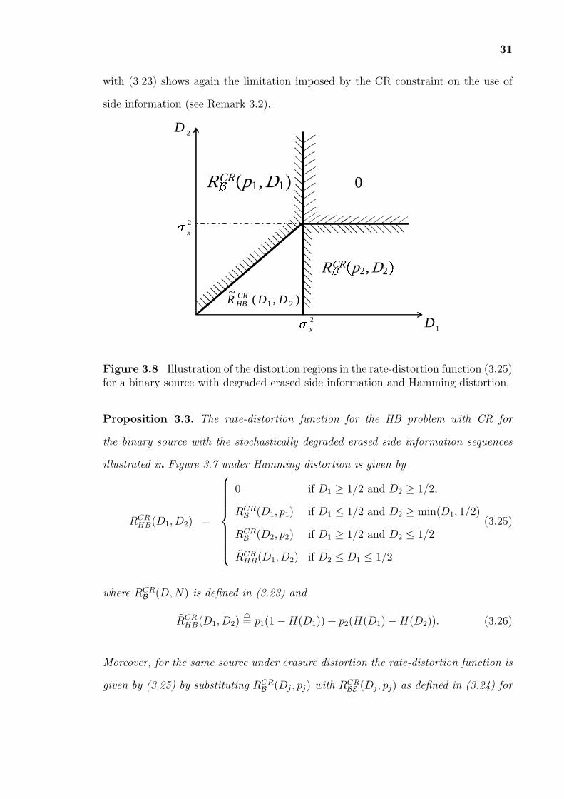
31
with (3.23) shows again the limitation imposed by the CR constraint on the use of
side information (see Remark 3.2).
1D2xσ
0
2
xσ2D
RBCRp2,D2),(
~21 DDR CR
HB
RBCRp1,D1
Figure 3.8 Illustration of the distortion regions in the rate-distortion function (3.25)for a binary source with degraded erased side information and Hamming distortion.
Proposition 3.3. The rate-distortion function for the HB problem with CR for
the binary source with the stochastically degraded erased side information sequences
illustrated in Figure 3.7 under Hamming distortion is given by
RCRHB(D1, D2) =
0 if D1 ≥ 1/2 and D2 ≥ 1/2,
RCRB (D1, p1) if D1 ≤ 1/2 and D2 ≥ min(D1, 1/2)
RCRB (D2, p2) if D1 ≥ 1/2 and D2 ≤ 1/2
RCRHB(D1, D2) if D2 ≤ D1 ≤ 1/2
(3.25)
where RCRB (D,N) is defined in (3.23) and
RCRHB(D1, D2)
△= p1(1−H(D1)) + p2(H(D1)−H(D2)). (3.26)
Moreover, for the same source under erasure distortion the rate-distortion function is
given by (3.25) by substituting RCRB (Dj, pj) with R
CRBE (Dj, pj) as defined in (3.24) for

32
j = 1, 2 and by substituting (3.26) with
RCRHB,E(D1, D2)
△= p1(1−D1) + p2(D1 −D2). (3.27)
Similar to the Gaussian example, the characterization of the rate distortion
function (3.25) requires different considerations for the four subregions of the (D1, D2)
plane sketched in Figure 3.8. In fact, for D1 ≥ 1/2 and D2 ≥ 1/2, the required rate
is zero, since the distortion constraints are trivially met by setting X1 = X2 = 0 in
the achievable rate (3.11). For the case D1 ≥ 1/2 and D2 ≤ 1/2, it is sufficient to
cater only to Decoder 2 by setting X1 = 0 and X = X2 ⊕ Q2, with Q2 ∼ Ber(D2)
independent of X, in the achievable rate (3.11). That this rate cannot be improved
upon is a consequence from the trivial converse
RCRHB(D1, D2) ≥ max{RCR
B (D1, p1), RCRB (D2, p2)}, (3.28)
which follows by cut-set arguments. The same converse suffices also for the regime
D1 ≤ 1/2 and D2 ≥ min(D1, 1/2). For this case, achievability follows by setting
X = X1 ⊕ Q1 and X1 = X2 in (3.11), where Q1 ∼ Ber(D1) is independent of X1.
In the remaining case, namely D2 ≤ D1 ≤ 1/2, the rate-distortion function does not
follow from the point-to-point result (3.23) as for the regimes discussed thus far. The
analysis of this case can be found in Appendix D. Similar arguments apply also for
the erasure distortion metric.
The rate-distortion function for the binary source X ∼ Ber(12) is now compared
with erased side information under Hamming distortion for three settings. In the
first setting, known as the Kaspi model [9], the encoder knows the side information,
and thus the position of the erasures. For this case, the rate-distortion function
RKaspi(D1, D2) for the example at hand was calculated in [19]. Note that in the
Kaspi model, the CR constraint does not affect the rate-distortion performance since
the encoder has all the information available at the decoders. The second model

33
of interest is the standard HB setting with no CR constraint, whose rate-distortion
function RHB(D1, D2) for the example at hand was derived [14]. The third model is
the HB setup with CR studied here. The inequalities
RKaspi(D1, D2) ≤ RHB(D1, D2) ≤ RCRHB(D1, D2), (3.29)
hold, where the first inequality in (3.29) accounts for the impact of the availability
of the side information at the encoder, while the second reflects the potential
performance loss due to the CR constraint.
Figure 3.9 shows the aforementioned rate-distortion functions with p1 = 1 and
p2 = 0.35, which corresponds to the case where Decoder 1 has no side information,
for two values of the distortion D2 versus the distortion D1. For D2 ≥ p22= 0.175, the
given settings reduce to one in which the encoder needs to communicate information
only to Decoder 1. Since Decoder 1 has no side information, the Kaspi and HB
settings yield equal performance i.e., RKaspi(D1, D2) = RHB(D1, D2). Moreover,
if D1 is sufficiently smaller than D2, the operation of the encoder is limited by
the distortion requirements of Decoder 1. In this case, Decoder 2 can in fact
reconstruct as X1 = X2 while still satisfying its distortion constraints. Therefore,
the same performance is obtained in all of the three settings, i.e., RKaspi(D1, D2) =
RHB(D1, D2) = RCRHB(D1, D2). It is also noted that the general performance loss due
to the CR constraint, unless, as discussed above, distortion D1 is sufficiently smaller
than D2.
3.3 Heegard-Berger Problem with Cooperative Decoders
The system model for the HB problem with CR and decoder cooperation is similar to
the one provided in Section 3.2.1 with the following differences. Here, in addition to
encoding function given in (8.33) which maps the source sequence Xn into a message

34
0 0.05 0.1 0.15 0.2 0.25 0.3 0.35 0.4 0.45 0.50
0.1
0.2
0.3
0.4
0.5
0.6
0.7
0.8
0.9
D1
R(D
1,D
2)
RKaspi
RHB
RHBCR
D2=0.3
D2=0.05
Figure 3.9 Rate-distortion functions RKaspi(D1, D2) [19], RHB(D1, D2) [14] andRCR
HB(D1, D2) (3.25) for a binary source under erased side information versus distortionD1 (p1 = 1, p2 = 0.35, D2 = 0.05 and D2 = 0.3).
J1 of nR1 bits, there is an encoder at Decoder 1 given by
g1: [1, 2nR1 ]× Yn
1 → [1, 2nR2 ], (3.30)
which maps message J1 and the source sequence Y n1 into a message J2. Moreover,
instead of the decoding function given in (3.5), the decoding function for Decoder 2
is
h2: [1, 2nR1 ]× [1, 2nR2 ]× Yn
2 → X n2 , (3.31)
which maps the messages J1 and J2 and the side information Y n2 into the estimated
sequence Xn2 .

35
3.3.1 Rate-Distortion Region for X − Y1 − Y2
In this section, a single-letter characterization of the rate-distortion region is derived
under the assumption that the joint pmf p(x, y1, y2) is such that the Markov chain
X − Y1 − Y2 holds3.
Proposition 3.4. The rate-distortion region RCR(D1, D2) for the HB source coding
problem with CR and cooperative decoders under the assumption X −Y1−Y2 is given
by the union of all rate pairs (R1, R2) that satisfy the conditions
R1 ≥ I(X; X1X2|Y1) (3.32a)
and R1 +R2 ≥ I(X; X2|Y2) + I(X; X1|Y1, X2), (3.32b)
where the mutual information terms are evaluated with respect to the joint pmf
p(x, y1, y2, x1, x2) = p(x, y1)p(y2|y1)p(x1, x2|x), (3.33)
for some pmf p(x1, x2|x) such that the constraints (3.13) are satisfied.
The proof of the converse can be easily established following cut-set arguments
for bound (3.32a), while the bound (3.32b) on the sum-rate R1 + R2 can be proved
following the same step as in Appendix A and substituting J with (J1, J2). As for
the achievability, it follows as a straightforward extension of [10, Section III] to the
setup at hand where Decoder 2 has side information as well. It is worth emphasizing
that the reconstruction X2 for the Decoder 2, which has degraded side information,
is conveyed by using both the direct link from the Encoder, of rate R1, and the
path Encoder-Decoder 1-Decoder 2. The latter path leverages the the better side
information at Decoder 1 and the cooperative link of rate R2.
3Note that, unlike the conventional HB problem studied in Section 3.2, the rate-distortionregion with cooperative decoders depends on the joint distribution of the variables (Y1, Y2),and thus stochastic and physical degradedness of the side information sequences lead todifferent results.

36
Remark 3.7. Without the CR constraint, the problem of determining the rate-
distortion region for the setting of Figure 3.3 under the assumption X − Y1 − Y2
is still open. In [10], inner and outer bounds are obtained to the rate distortion
region, for the case which the side information Y2 is absent. The bounds were shown
to coincide for the case where Decoder 1 wishes to recover X losslessly (i.e., D1 = 0)
and also for certain distortion regimes in the quadratic Gaussian case. Moreover,
the rate distortion tradeoff is completely characterized in [10] for the case in which
the encoder also has access to the side information. It is noted that, as per the
discussion in Section 3.2.4, these latter result immediately carry over to the case with
CR constraint since the encoder is informed about the side information.
Remark 3.8. To understand why imposing the CR constraint simplifies the problem
of obtaining a single-letter characterization of the rate-distortion function, let us
consider the degrees of freedom available at Decoder 1 in Figure 3.3 for the use of
the link of rate R2. In general, Decoder 1 can follow two possible strategies: the first
is forwarding, whereby Decoder 1 simply forwards some of the bits received from the
encoder to Decoder 2; while the second is recompression, whereby the data received
from the encoder is combined with the available side information Y n1 , compressed
to at most R2 bits per symbol, and then sent to Decoder 2. It is the interplay and
contrast between these two strategies that makes the general problem hard to solve. In
particular, while the strategies of forwarding/recompression and combinations thereof
appear to be natural candidates for the problem, finding a matching converse when
both such degrees of freedom are permissible at the decoder is difficult (see, e.g., [21]).
However, under the CR constraint, the strategy of recompression becomes irrelevant,
since any information about the side information Y n1 that is not also available at the
encoder cannot be leveraged by Decoder 2 without violating the CR constraint. This
restriction in the set of available strategies for Decoder 1 makes the problem easier
to address under the CR constraint.”

37
3.3.2 Rate-Distortion Region for X − Y2 − Y1
In this section, a single-letter characterization of the rate-distortion region is derived
under the assumption that the joint pmf p(x, y1, y2) is such that the Markov chain
relationship X − Y2 − Y1 holds.
Proposition 3.5. The rate-distortion region RCR(D1, D2) for the HB source coding
problem with CR and cooperative decoders under the assumption the Markov chain
relationship X − Y2 − Y1 is given by the union of all rate pairs (R1, R2) that satisfy
the conditions
R1 ≥ I(X; X1|Y1) + I(X; X2|Y2, X1) (3.34a)
and R2 ≥ 0, (3.34b)
where the mutual information terms are evaluated with respect to the joint pmf
p(x, y1, y2, x1, x2) = p(x, y2)p(y1|y2)p(x1, x2|x), (3.35)
for some pmf p(x1, x2|x) such that the constraints (3.13) are satisfied.
The proof of achievability follows immediately by neglecting the link of rate R2
and using rate R1 as per the HB scheme of Proposition 3.1. The converse follows
by considering an enhanced system in which Decoder 2 is provided with the side
information of Decoder 1. In this system, link R2 becomes useless since Decoder
2 possesses all the information available at Decoder 1. It follows that the system
reduces to the HB problem with degraded sources studied in the previous section and
the bound (3.34a) follows immediately from Proposition 3.1.
Remark 3.9. In the case without CR, the rate-distortion function is given similarly to
(3.34), but with the HB rate-distortion function (3.15) in lieu of the rate-distortion
function of the HB problem with CR in (3.34a).

38
3.4 Cascade Source Coding with Common Reconstruction
In this section, the system model in Figure 3.4 of cascade source coding with CR is first
detailed. As mentioned in Section 3.1, the motivation for studying this class of models
comes from multi-hop applications. Next, the characterization of the corresponding
rate-distortion performance is presented under the assumption that one of the two
side information sequences is a degraded version of the other. Finally, following the
previous section, three specific examples are worked out, namely Gaussian sources
under quadratic distortion (Section 3.4.3), and binary sources with side information
subject to erasures under Hamming or erasure distortion (Section 3.4.3).
3.4.1 System Model
In this section, the system model for the cascade source coding problem with CR is
detailed similar to Section 3.2.1. The problem is defined by the pmf pXY1Y2(x, y1, y2)
and discrete alphabets X ,Y1,Y2, X1, and X2 as follows. The source sequence Xn and
side information sequences Y n1 and Y n
2 , with Xn ∈ X n, Y n
1 ∈ Yn1 , and Y
n2 ∈ Yn
2 are
such that the tuples (Xi, Y1i, Y2i) for i ∈ [1, n] are i.i.d. with joint pmf pXY1Y2(x, y1, y2).
Node 1 measures a sequence Xn and encodes it into a message J1 of nR1 bits, which
is delivered to Node 2. Node 2 estimates a sequence Xn1 ∈ X n
1 within given distortion
requirements. Node 2 also encodes the message J1 received from Node 1 and the
sequence Y n1 into a message J2 of nR2 bits, which is delivered to Node 3. Node 3
estimates a sequence Xn2 ∈ X n
2 within given distortion requirements. Distortion and
CR requirements are defined as in Section 3.2.1, leading to the following definition.
Definition 3.2. An (n,R1, R2, D1, D2, ϵ) code for the cascade source coding problem
with CR consists an encoding function for Node 1,
g1: X n → [1, 2nR1 ], (3.36)
39
which maps the source sequence Xn into a message J1; an encoding function for Node
2,
g2: [1, 2nR1 ]× Yn
1 → [1, 2nR2 ], (3.37)
which maps the source sequence Y n1 and message J1 into a message J2; a decoding
function for Node 2
h1: [1, 2nR1 ]× Yn
1 → X n1 , (3.38)
which maps message J1 and the side information Y n1 into the estimated sequence Xn
1 ;
a decoding function for Node 3
h2: [1, 2nR2 ]× Yn
2 → X n2 , (3.39)
which maps message J2 and the side information Y n2 into the estimated sequence
Xn2 ; two encoder reconstruction functions as in (3.7), which map the source sequence
into estimated sequences ψ1(Xn) and ψ2(X
n) at Node 1; such that the distortion
constraints (3.8) and (3.9) are satisfied.
Given a distortion pair (D1, D2), a rate pair (R1, R2) is said to be achievable if,
for any ϵ > 0 and sufficiently large n, there a exists an (n,R1, R2, D1 + ϵ,D2 + ϵ, ϵ)
code. The rate-distortion region R(D1, D2) is defined as the closure of all rate pairs
(R1, R2) that are achievable given the distortion pair (D1, D2).
3.4.2 Rate-Distortion Region for X − Y1 − Y2
In this section, a single-letter characterization of the rate-distortion region is derived
under the assumption that the joint pmf p(x, y1, y2) is such that the Markov chain
relationship X − Y1 − Y2 holds 4.
4As for the HB problem with cooperative decoders studied in Section 3.3, the rate-distortionregion of the cascade source coding problem depends on the joint distribution of the variables
40
Proposition 3.6. The rate-distortion region RCR(D1, D2) for the cascade source
coding problem with CR is given by the union of all rate pairs (R1, R2) that satisfy
the conditions
R1 ≥ I(X; X1X2|Y1) (3.40a)
and R2 ≥ I(X; X2|Y2), (3.40b)
where the mutual information terms are evaluated with respect to the joint pmf
p(x, y1, y2, x1, x2) = p(x, y1)p(y2|y1)p(x1, x2|x), (3.41)
for some pmf p(x1, x2|x) such that the constraints (3.13) are satisfied.
The proof of the converse is easily established following cut-set arguments. To
prove achievability, it is sufficient to consider a scheme based on binning at Node 1
and decode and rebin at Node 2 (see [13]). Specifically, Node 1 randomly generates a
standard lossy source code Xn1 for the source Xn with rate I(X; X1) bits per source
symbol. Random binning is used to reduce the rate to I(X; X1|Y1). Node 1 then
maps the source Xn into the reconstruction sequence Xn2 using a codebook that is
generated conditional on Xn1 with rate I(X; X2|X1) bits per source symbol. Using
the side information Y n1 available at Node 2, random binning is again used to reduce
the rate to I(X; X2|Y1X1). The codebook of Xn2 is also randomly binned to the rate
I(X; X2|Y2). Node 2, having recovered Xn2 , forwards the corresponding bin index
to Node 3. The latter, by choice of the binning rate, is able to obtain Xn2 . Note
that, since the reconstruction sequences Xn1 and Xn
2 are generated by the encoder,
functions ψ1 and ψ2 that guarantees the CR constraints (3.9) exist by construction.
Remark 3.10. Without the CR constraint, the problem of determining the rate-
distortion region for the setting of Figure 3.4 under the Markov condition X−Y1−Y2
(Y1, Y2), and thus stochastic and physical degradedness of the side information sequenceslead to different results.

41
is still open. In the special case in which Y1 = Y2 the problem has been solved in [12]
for Gaussian sources under quadratic distortion and in [14] for binary sources with
erased side information under Hamming distortion.
Remark 3.11. Following Remark 3.3, if both side information sequences are causal,
it can be shown that they have no impact on the rate-distortion function (3.40).
Therefore, the rate-distortion region follows immediately from the results in (3.40) by
removing both of the side information terms. Note that with causal side information
sequences the rate-distortion function holds for any joint pmf p(x, y1, y2) with no
degradedness requirements. Moreover, if only the side information Y2 is causal, while
Y1 is still observed non-causally, then the side information Y2 can be neglected without
loss of optimality, and the rate-distortion region follows from (3.40) by removing the
conditioning on Y2.
3.4.3 Bounds on the Rate-Distortion Region for X − Y2 − Y1
In this section, outer and inner bounds are derived for the rate-distortion region
under the assumption that the joint pmf p(x, y1, y2) is such that the Markov chain
relationship X − Y2 − Y1 holds. The bounds are then shown to coincide in Section
3.4.3 for Gaussian sources and in Section 3.4.3 for binary sources with erased side
information.
Proposition 3.7. (Outer bound) The rate-distortion region RCR(D1, D2) for the
cascade source coding problem with CR is contained in the region RCRout (D1, D2), which
is given by the set of all rate pairs (R1, R2) that satisfy the conditions
R1 ≥ RCRHB(D1, D2) (3.42a)
and R2 ≥ RCRX|Y2
(D2), (3.42b)
42
where RCRHB(D1, D2) is defined in (3.11) and RCR
X|Y2(D2) = min I(X; X2|Y2), where
the minimization is performed with respect to the conditional pmf p(x2|x) under the
distortion constraints (3.13) for j = 2.
Proposition 3.8. (Inner bound) The rate-distortion region RCR(D1, D2) for the
cascade source coding problem with CR contains the region RCRin (D1, D2), which is
given by the union of all rate pairs (R1, R2) that satisfy the conditions
R1 ≥ I(X; X1|Y1) + I(X; X2|Y2X1) (3.43a)
and R2 ≥ I(X; X1|Y2) + I(X; X2|X1Y2) (3.43b)
= I(X; X1X2|Y2) (3.43c)
where the mutual information terms are evaluated with respect to the joint pmf
p(x, y1, y2, x1, x2) = p(x, y2)p(y1|y2)p(x1, x2|x), (3.44)
for some pmf p(x1, x2|x1) such that the distortion constraints (3.13) are satisfied.
The outer bound in Proposition 3.7 follows immediately from cut-set arguments
similar to those in [12] and [14]. As for the inner bound of Proposition 19, the strategy
works as follows. Node 1 sends the description Xn1 to Node 2 using binning with rate
I(X; X1|Y1). It also maps the sequence Xn into the sequence Xn2 using a conditional
codebook with respect to Xn1 , which is binned in order to leverage the side information
Y n2 at Node 3 with rate I(X; X2|X1, Y2). Node 2 recovers X
n1 , whose codebook is then
binned to rate I(X; X1|Y2). Then, it forwards the so obtained bin index for Xn1 and
the bin index for the codebook of Xn2 produced by Node 1 to Node 3. By the choice
of the rates, the latter can recover both Xn1 and Xn
2 . Since both descriptions are
produced by Node 1, the CR constraint is automatically satisfied.

43
The inner and outer bounds defined above do not coincide in general. However,
in the next sections, two examples are provided in which they coincide and thus
characterize the rate-distortion region of the corresponding settings.
Remark 3.12. Without the CR constraint, the problem of deriving the rate-distortion
region for the setting at hand under the Markov chain condition X −Y2−Y1 is open.
The problem has been solved in [12] for Gaussian sources under quadratic distortion
and in [14] for binary sources with erased side information under Hamming distortion
for Y1 = Y2.
Gaussian Sources and Quadratic Distortion In this section, Gaussian sources
in (3.17) and the quadratic distortion are assumed as in Sec 3.2.3, and derive the
rate-distortion region for the cascade source coding problem with CR.
Proposition 3.9. The rate-distortion region RCR(D1, D2) for the cascade source
coding problem with CR for the Gaussian sources in (3.17) and quadratic distortion
is given by (3.42) with RCRHB(D1, D2) in (3.19) and RCR
X|Y2(D2) = RCR
G (D2, N2) (see
(3.18)).
The proof is given in Appendix E.
Binary Sources with Erased Side Information and Hamming Distortion
In this section, the binary sources in Figure 3.7 and the Hamming distortion are
assumed as in Sec 3.2.4, and derive the rate-distortion region for the cascade source
coding problem with CR.
Proposition 3.10. The rate-distortion region RCR(D1, D2) for the cascade source
coding problem with CR for the binary sources in Figure 3.7 and Hamming distortion
is given by (3.42) with RCRHB(D1, D2) in (3.25) and RCR
X|Y2(D2) = RCR
B (D2, p2) (see
(3.23)).
The proof is given in Appendix F.

44
3.5 Heegard-Berger Problem with Constrained Reconstruction
In this section, the HB problem is revisited and relax the CR constraint to the ConR
constraint of [13]. This implies that the code as per Definition 1 is still adopted, but
(3.9) is substituted with the less stringent constraint
1
n
n∑i=1
E[de,j(Xji, ψji(X
n))]≤ De,j for j = 1, 2, (3.45)
where de,j(xj, xe,j): Xj × Xj → [0, De,max] is a per-symbol distortion metric and
ψji(Xn), for j = 1, 2 is used to denote the ith letter of the vector ψj(X
n) =
(ψj1(Xn), ..., ψjn(X
n)).
Definition 3.3. Given a distortion tuple (De,1, De,2, D1, D2), a rate R is said to be
achievable if, for any ϵ > 0 and sufficiently large n, there a exists an (n,R,De,1 +
ϵ,De,2+ ϵ,D1+ ϵ,D2+ ϵ, ϵ) code. The rate-distortion function R(De,1, De,2, D1, D2) is
defined as R(De,1, De,2, D1, D2) = inf{R: the tuple (De,1, De,2, D1, D2) is achievable}.
Note that, by setting De,j = 0 for j = 1, 2, and letting de,j(xj, xe,j) be the
Hamming distortion metric (i.e., de,j(xj, xe,j) = 1 if x = xj and de,j(xj, xe,j) = 0
if x = xj), a relaxed CR constraint is obtained in which the average per-symbol,
rather than per-block, error probability criterion is adopted.
Remark 3.13. The problem at hand reduces to the one studied in [15] by setting
D1 = Dmax and De,1 = De,max.
Proposition 3.11. If the side information Y1 is stochastically degraded with respect
to Y2, the rate-distortion function for the HB problem with ConR is given by
RConRHB (De,1, De,2, D1, D2) = min I(X;U1|Y1) + I(X;U2|Y2U1) (3.46a)
= min I(X;U1U2|Y2) + I(U1;Y2|Y1), (3.46b)
where the mutual information terms are evaluated with respect to the joint pmf
p(x, y1, y2, u1, u2) = p(x, y1, y2)p(u1, u2|x), (3.47)

45
and minimization is performed with respect to the conditional pmf p(u1, u2|x) and
the deterministic functions xj(uj, yj): Uj × Yj → Xj and xe,j(uj, x): Uj ×X → Xe,j
for j = 1, 2, such that the distortion constraints E[dj(X, xj(Uj, Yj))] ≤ Dj for j = 1, 2,
and the ConR requirements
E[de,j(xj(Uj, Yj), xe,j(Uj, X))] ≤ De,j, for j = 1, 2, (3.48)
are satisfied. Finally, (U1, U2) are auxiliary random variables whose alphabet
cardinalities can be constrained as |U1| ≤ |X |+ 4 and |U2| ≤ (|X |+ 2)2.
The proof is given in Appendix G.
Remark 3.14. Proposition 3.11 reduces to [15, Theorem 2] when setting D1 = Dmax
and De,1 = De,max.
Remark 3.15. Similar to [15, Theorem 2], it can be proved that, by setting De,1 =
De,2 = 0 and letting de,j be the Hamming distortion for j = 1, 2, the rate-distortion
function (3.46), RConRHB (0, 0, D1, D2), reduces to the rate-distortion function with CR
(3.11).
Remark 3.16. Similar to Remark 3.15, if De,1 = 0 and De,2 = De,max, the rate-
distortion function (3.46) is given by
RCRHB(0, De,max, D1, D2) = min I(X; X1|Y1) + I(X;U2|Y2X1), (3.49)
where the mutual information terms are evaluated with respect to the joint pmf
p(x, y1, y2, u2, x1) = p(x, y1, y2)p(x1, u2|x), (3.50)
and minimization is performed with respect to the conditional pmf p(x1, u2|x) and the
deterministic functions x2(u2, y2): U2 × Y2 → X2 and xe,2(u2, x): U2 ×X → Xe,2, such
that the distortion constraints E[d1(X, X1)] ≤ D1 and E[d2(X, x2(U2, Y2))] ≤ D2 and
the ConR requirement E[de,2(x2(U2, Y2), xe,2(U2, X))] ≤ De,2 are satisfied. It can be

46
proved that this is also the rate-distortion function under the partial CR requirement
that there exists a function ψ1(Xn) such that (3.9) holds for j = 1 only. Similar
conclusions apply symmetrically to the case where CR and ConR requirements are
imposed only on the reconstruction of Decoder 2.
Remark 3.17. If both side information sequences are causally available at the
decoders, it can be proved that they have no impact on the rate-distortion function
(3.46). In this case, the rate-distortion function follows immediately from the results
in (3.46) by removing conditioning on both side information sequences. Moreover, the
result can be simplified by introducing a single auxiliary random variable. Similarly, if
only side information Y1 is causal, then it can be neglected with no loss of optimality,
and the results follow from (3.46) by removing the conditioning on Y1.
Remark 3.18. It is noted that the ConR formulation studied in this section is more
general than the conventional formulation with distortion constraints for the decoders
only. Therefore, problems that are open with the conventional formulation, such as
HB with cooperative decoders (Section 3.3) and cascade source coding (Section 3.4),
are a fortiori also open in the ConR set-up.
3.6 Concluding Remarks
The Common Reconstruction requirement [8], and its generalization in [15], substan-
tially modify the problem of source coding in the presence of side information at the
decoders. From a practical standpoint, in various applications, such as transmission
of medical records, CR is a design constraint. In these cases, evaluation of the
rate-distortion performance under CR thus reveals the cost, in terms of transmission
resources, associated with this additional requirement. From a theoretical perspective,
adding the CR constraint to standard source coding problems with decoder side
information proves instrumental in concluding about the optimality of various known
strategies in settings in which the more general problem, without the CR constraint,

47
is open [8]. This chapter has extended these considerations from a point-to-point
setting to three baseline multiterminal settings, namely the Heegard-Berger problem,
the HB problem with cooperating decoders and the cascade problems. The optimal
rate-distortion trade-off has been derived in a number of cases and explicitly evaluated
in various examples.
A general subject of theoretical interest is identifying those models for which
the CR requirements enables a solution of problems that have otherwise resisted
solutions for decades. Examples include the Heegard-Berger and cascade source
coding problems with no assumptions on side information degradedness and the
one-helper lossy source coding problem.

CHAPTER 4
DISTRIBUTED AND CASCADE SOURCE CODING WITH SIDE
INFORMATION “VENDING MACHINE”
4.1 Introduction
As reviewed in Chapter 2, reference [4] introduced the notion of a side information
“vending machine”. To illustrate the idea, consider the setting in Figure 4.1, as
studied in [4]. Here, as explained in Chapter 2, unlike the conventional Wyner-Ziv
set-up (see, e.g., [1, Chapter 12]), the joint distribution of the side information Y n
available at the decoder (Node 2) and of the source Xn observed at the encoder (Node
1) is not given. Instead, it can be controlled through the selection of an “action”
An, so that, for a given action An and source symbol Xn, the side information Y n
is distributed according to a given conditional distribution p(y|a, x). Action An is
selected by the decoder based on the messageM , of R bits per source symbol, received
from the encoder, and is subject to a cost constraint. The latter limits the “quality”
of the side information that can be collected by the decoder.
The source coding problem with a vending machine provides a useful model
for scenarios in which acquiring data as side information is costly and thus should
be done effectively. Examples include computer networks, in which data must be
obtained from remote data bases, and sensor networks, where data is acquired via
measurements.
The key aspect of this model is that the message M produced by the encoder
plays a double role. In fact, on the one hand, it needs to carry the description of the
source Xn itself, as in, e.g., the standard Wyner-Ziv model. On the other hand, it can
also carry control information aimed at enabling the decoder to make an appropriate
selection of action An. The goal of such a selection is to obtain a side information
48

49
Y n that is better suited to provide partial information about the source Xn to the
decoder. This in turn can potentially reduce the rate R necessary for the decoder
to reconstruct source Xn at a given distortion level (or, vice versa, to reduce the
distortion level for a given rate R).
The performance of the system in Figure 4.1 is expressed in terms of the
interplay among three metrics, namely the rate R, the cost budget Γ on the action
An, and the distortion D of the reconstruction X at the decoder. This trade-off is
summarized by the rate-distortion-cost function R(D,Γ). This function characterizes
the infimum of all rates R for which a distortion level D can be achieved under
an action cost budget Γ, by allowing encoding of an arbitrary number n of source
symbols Xn = (X1, ..., Xn). This function is derived in [4] for both cases in which the
side information Y n is available “non-causally” to the decoder, as in the standard
Wyner-Ziv model, or “causally”, as introduced in [16]. In the former case (Figure
4.1-(a)), the estimated sequence Xn = (X1, ..., Xn) is a function of message M
and of the entire side information sequence Y n = (Y1, ..., Yn), while, in the latter
(Figure 4.1-(b)), each estimated sample Xi is a function of message M and the side
information as received up to time i, i.e., Y i = (Y1, ..., Yi) for i = 1, ..., n. It is noted
that the model with causal side information is appropriate, for instance, when there
are delay constraints on the reproduction at the decoder or when the decoder operates
by filtering the side information sequence. The reader is referred to [16, Sec I] for an
extensive discussion on these points.
Following reference [4], recent works [22] and [23] generalized the characteri-
zation of the rate-distortion-cost function for the models in Figure 4.1 to a set-up
analogous to the so called Kaspi-Heegard-Berger problem [3][9], in which the side
information vending machine may or may not be available at the decoder. This
entails the presence of two decoders, rather than only one as in Figure 4.1, one with
access to the vending machine and one without any side information. Reference [23]

50
Node 1
nA
ˆ nX
( | , )p y a x
Node 2R
nX
nY
nX
( )a
Node 1
nA
ˆiX
( | , )p y a x
Node 2R
nX
iY
nX
( )b
Figure 4.1 Source coding with a vending machine at the decoder [4] with: (a)“non-causal” side information; (b) “causal” side information.
also solved the more general case in which both decoders have access to the same
vending machine, and either the side informations produced by the vending machine
at the two decoders satisfy a degradedness condition, or lossless source reconstructions
are required at the decoders. The papers [24][25] studied the setting of Figure 4.1
but under the additional constraints of common reconstruction, in the sense of [8],
in [24], and of secrecy with respect to an “eavesdropping” node in [25], providing
characterizations of the corresponding achievable performance. The impact of actions
that adapt to the previously measured samples of the side information is studied in
[26]. In [27], a related problem is considered in which the sequence to be compressed is
dependent on the actions taken by a separate encoder. Finally, real-time constraints
are investigated in [28].
4.1.1 Contributions and Overview
In this chapter, two multi-terminal extensions of the set-up in Figure 4.1 are studied,
namely the distributed source coding setting of Figure 4.2, and the cascade model of
Figure 4.3. The analysis of these scenarios is motivated by the observation that they

51
constitute key components of computer and sensor networks. In fact, as discussed
above, an important aspect of these networks is the need to effectively acquire side
information data, which can be modeled by including a side information vending
machine. The two extensions and the corresponding main results are evaluated below.
1) Distributed source coding with a side information vending machine (Section
4.2): In the distributed source coding setting of Figure 4.2, two encoders (Node 1 and
Node 2), which measure correlated sources Xn1 and Xn
2 , respectively, communicate
over rate-limited links, of rates R1 and R2, respectively, to a single decoder (Node 3).
The decoder has side information Y n on sources Xn1 and Xn
2 , which can be controlled
through an action An. The action sequence is selected by the decoder based on the
messages M1 and M2 received from Node 1 and Node 2, respectively, and needs to
satisfy a cost constraint of Γ. Inner bounds are derived to the rate-distortion-
Node 1nX1
nA
),,|( 21 xxayp
nYnX 2 Node 2 2R
1R
Node 3nX1
ˆ
nX 2ˆ
nX1nX 2
Figure 4.2 Distributed source coding with a side information vending machine atthe decoder.
Node 2Node 1nX1
nA
12RiX 2
ˆ
),,|( 21 xxayp
iY
Node 323R
nX1ˆ
nX 2nX1nX 2
Figure 4.3 Cascade source coding with a side information vending machine. Sideinformation is assumed to be available “causally” to the decoder.
cost region R(D1, D2,Γ) under non-causal and causal side information by combining
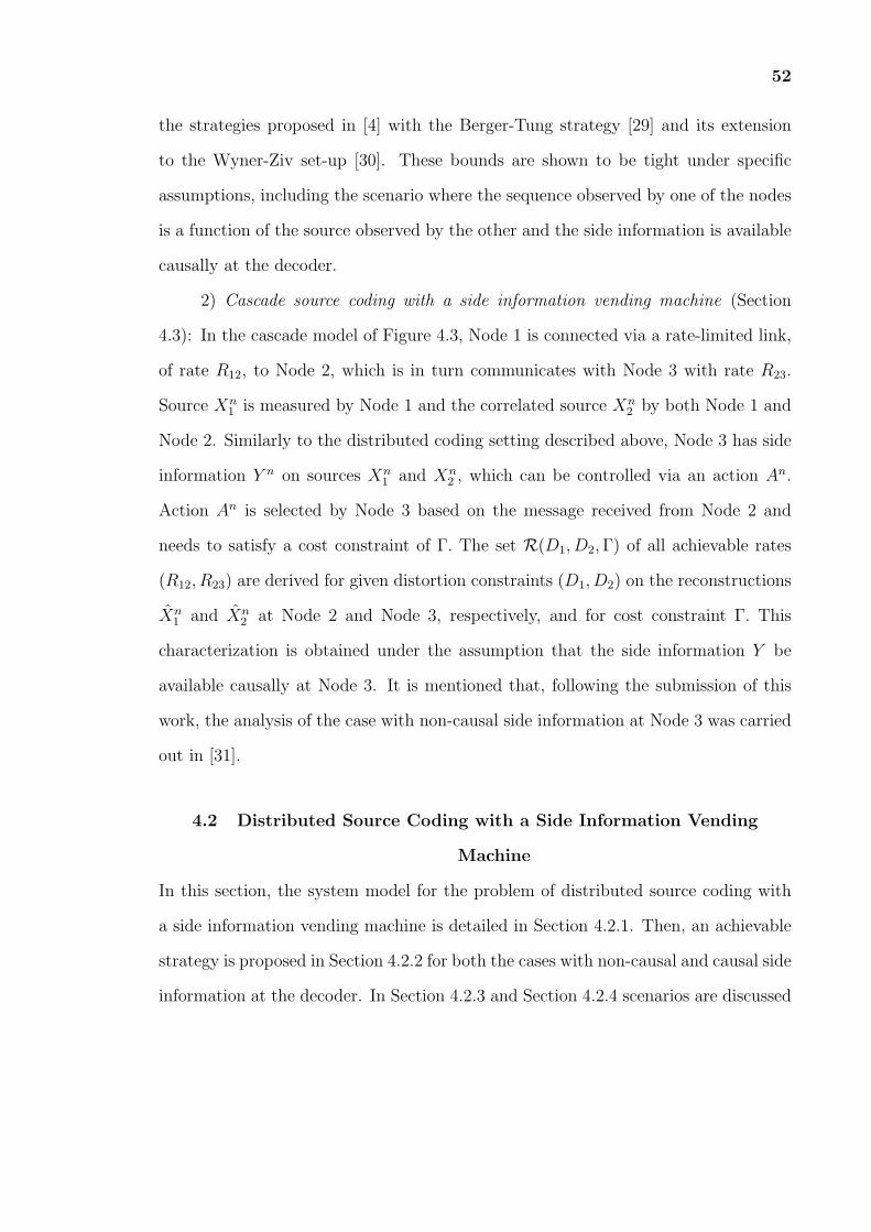
52
the strategies proposed in [4] with the Berger-Tung strategy [29] and its extension
to the Wyner-Ziv set-up [30]. These bounds are shown to be tight under specific
assumptions, including the scenario where the sequence observed by one of the nodes
is a function of the source observed by the other and the side information is available
causally at the decoder.
2) Cascade source coding with a side information vending machine (Section
4.3): In the cascade model of Figure 4.3, Node 1 is connected via a rate-limited link,
of rate R12, to Node 2, which is in turn communicates with Node 3 with rate R23.
Source Xn1 is measured by Node 1 and the correlated source Xn
2 by both Node 1 and
Node 2. Similarly to the distributed coding setting described above, Node 3 has side
information Y n on sources Xn1 and Xn
2 , which can be controlled via an action An.
Action An is selected by Node 3 based on the message received from Node 2 and
needs to satisfy a cost constraint of Γ. The set R(D1, D2,Γ) of all achievable rates
(R12, R23) are derived for given distortion constraints (D1, D2) on the reconstructions
Xn1 and Xn
2 at Node 2 and Node 3, respectively, and for cost constraint Γ. This
characterization is obtained under the assumption that the side information Y be
available causally at Node 3. It is mentioned that, following the submission of this
work, the analysis of the case with non-causal side information at Node 3 was carried
out in [31].
4.2 Distributed Source Coding with a Side Information Vending
Machine
In this section, the system model for the problem of distributed source coding with
a side information vending machine is detailed in Section 4.2.1. Then, an achievable
strategy is proposed in Section 4.2.2 for both the cases with non-causal and causal side
information at the decoder. In Section 4.2.3 and Section 4.2.4 scenarios are discussed

53
in which the achievable strategies match given outer bounds. A numerical example
is then developed in Section 4.2.5.
4.2.1 System Model
The problem of distributed lossy source coding with a vending machine and non-
causal side information is illustrated in Figure 4.2. It is defined by the probability
mass functions (pmfs) pX1X2(x1, x2) and pY |AX1X2(y|a, x1, x2) and discrete alphabets
X1,X2,Y ,A, X1, X2 as follows. The source sequences Xn1 and Xn
2 with Xn1 ∈ X n
1
and Xn2 ∈ X n
2 , respectively, are such that the tuples (X1i, X2i) for i ∈ [1, n] are
independent identically distributed (i.i.d.) with joint pmf pX1X2(x1, x2). Node 1
measures sequences Xn1 and encodes it into message M1 of nR1 bits, while Node 2
measures sequences Xn2 and encodes it into message M2 of nR2 bits. Node 3 wishes
to reconstruct the two sources within given distortion requirements, to be discussed
below, as Xn1 ∈ X n
1 and Xn2 ∈ X n
2 .
To this end, Node 3 selects an action sequence An, where An ∈ An, based
on the messages M1 and M2 received from Node 1 and Node 2, respectively. The
side information sequence Y n is then realized as the output of a memoryless channel
with inputs (An, Xn1 , X
n2 ). Specifically, given An, Xn
1 and Xn2 , the sequence Y n is
distributed as
p(yn|an, xn1 , xn2 ) =n∏
i=1
pY |AX1X2(yi|ai, x1i, x2i). (4.1)
The overall cost of an action sequence an is defined by a per-symbol cost function Λ:
A →[0,Λmax] with 0 ≤ Λmax <∞, as
Λn(an) =1
n
n∑i=1
Λ(ai). (4.2)
The estimated sequences Xn1 and Xn
2 are obtained as a function of both messages M1
andM2 and of the side information Y n. The estimates Xn1 and Xn
2 are constrained to

54
satisfy distortion constraints defined by two per-symbol distortion measures, namely
dj(x1, x2, y, xj): X1×X2×Y×Xj → [0, Dmax] for j = 1, 2 with 0 ≤ Dmax <∞. Based
on such scalar measures, the overall distortion for the estimated sequences xn1 and xn2
is defined as
dnj (xn1 , x
n2 , y
n, xnj ) =1
n
n∑i=1
dj(x1i, x2i, yi, xji) for j = 1, 2. (4.3)
Note that, based on (4.3), the estimate Xnj for j = 1, 2 can be required to be a lossy
version of an arbitrary (per-letter) function of both sources Xn1 and Xn
2 and of the
side information sequence Y n. A formal description of the operations at encoders and
decoder, and of cost and distortion constraints, is presented below for both the cases
in which the side information is available causally or non-causally at the decoder.
Definition 4.1. An (n,R1, R2, D1, D2,Γ) code for the case of non-casual side
information at Node 3 consists of two source encoders
g1: X n1 → [1, 2nR1 ],
and g2: X n2 → [1, 2nR2 ], (4.4)
which map the sequences Xn1 and Xn
2 into messages M1 and M2 at Node 1 and Node
2, respectively; an “action” function
ℓ: [1, 2nR1 ]× [1, 2nR2 ] → An, (4.5)
which maps the message (M1,M2) into an action sequence An at Node 3; and two
decoding functions
h1: [1, 2nR1 ]× [1, 2nR2 ]× Yn → X n
1 , (4.6)
and h2: [1, 2nR1 ]× [1, 2nR2 ]× Yn → X n
2 , (4.7)

55
which map the messages M1 and M2, and the side information sequence Y n into the
estimated sequences Xn1 and Xn
2 at Node 3; such that the action cost constraint Γ is
satisfied as
1
n
n∑i=1
E [Λ(Ai)] ≤ Γ, (4.8)
and the distortion constraints D1 and D2 hold, namely
1
n
n∑i=1
E[dj(X1i, X2i, Yi, Xji)
]≤ Dj, for j = 1, 2. (4.9)
Definition 4.2. A (n,R1, R2, D1, D2,Γ) code for the case of causal side information
at Node 3 is as in Definition 4.1 with the only difference that, in lieu of (6)-(7), the
sequence of decoding functions are
h1i: [1, 2nR1 ]× [1, 2nR2 ]× Y i → X1i, (4.10)
and h2i: [1, 2nR1 ]× [1, 2nR2 ]× Y i → X2i, (4.11)
for i ∈ [1, n], which map the message (M1,M2) and the measured sequence Y i into
the ith estimated symbol Xji = hji(M1,M2, Yi) for j = 1, 2 at Node 3.
Definition 4.3. Given a distortion-cost tuple (D1, D2,Γ), a rate pair (R1, R2) is said
to be achievable for the case with non-causal or causal side information if, for any ϵ > 0
and sufficiently large n, there exists a corresponding (n,R1, R2, D1 + ϵ,D2 + ϵ,Γ+ ϵ)
code.
Definition 4.4. The rate-distortion-cost region RNC(D1, D2,Γ) is defined as the
closure of all rate pairs (R1, R2) that are achievable with non-causal side infor-
mation given the distortion-cost tuple (D1, D2,Γ). The rate-distortion-cost region
RC(D1, D2,Γ) is similarly defined for the case of casual side information.

56
4.2.2 Achievable Strategies
In this section, inner bounds to the rate-distortion-cost regions are obtained for the
cases with non-causal and causal side information.
Proposition 4.1. The rate-distortion-cost region with non-causal side information
at Node 3 satisfies the inclusion RNC(D1, D2,Γ) ⊇ RaNC(D1, D2,Γ), where the region
RaNC(D1, D2,Γ) is given by the union of the set of all of rate tuples (R1, R2) that
satisfy the inequalities
R1 ≥ I(X1;V1|V2, Q) + I(X1;U1|V1, V2, U2, Y,Q) (4.12a)
R2 ≥ I(X2;V2|V1, Q) + I(X2;U2|V1, V2, U1, Y,Q) (4.12b)
and R1 +R2 ≥ I(X1, X2;V1, V2|Q) + I(X1, X2;U1, U2|V1, V2, Y,Q), (4.12c)
for some joint pmfs that factorizes as
p(q, x1, x2, y, v1, v2, u1, u2, a, x1, x2) =
p(q)p(x1, x2)p(v1, u1|x1, q)p(v2, u2|x2, q)δ(a− a(v1, v2, q))
p(y|a, x1, x2)δ(x1 − x1(u1, u2, y, q))δ(x2 − x2(u1, u2, y, q)), (4.13)
with pmfs p(q) and p(v1, u1|x1, q) and p(v2, u2|x2, q) and deterministic functions
a: V1×V2×Q → A, xj: U1×U2×Y ×Q→ Xj for j = 1, 2, such that the action and
the distortion constraints
E [Λ(A)] ≤ Γ (4.14a)
and E[dj(X1, X2, Y, Xj)
]≤ Dj, for j = 1, 2, (4.14b)
hold. Finally, any extreme point of the region RaNC(D1, D2,Γ) can be obtained by
limiting the cardinalities of the random variables (V1, V2, U1, U2) as |Vj| ≤ |Xj| + 6
and |Uj| ≤ |Xj| |Vj|+ 5, for j = 1, 2.

57
Remark 4.1. If p(y|a, x1, x2) = p(y|x1, x2), so that the side information is action-
independent, Proposition 4.1 reduces to the extension of the Berger-Tung scheme [29]
to the Wyner-Ziv set-up studied in [30, Theorem 2]. Moreover, in the special case in
which there is only one encoder, the achievable rate coincides with that derived in [4,
Theorem 1].
The proof of Proposition 4.1 follows easily from standard arguments, and thus
it is only briefly discussed here. The proposed scheme combines the Berger-Tung
distributed source coding strategy [29] and the distributed Wyner-Ziv approach
proposed in [30, Theorem II] with the layered two-stage coding scheme that is proved
to be optimal in [4] for the special case of a single encoder. Throughout the discussion,
the time-sharing variable is neglected Q for simplicity. This can be handled in the
standard way (see, e.g., [1, Section 4.5.3]). The encoding scheme at Node 1 and Node
2 multiplexes two descriptions, which are obtained in two encoding stages. In the
first encoding stage, the distributed source coding strategy of [29], conventionally
referred to as the Berger-Tung scheme, is adopted by Node 1 and Node 2 to convey
descriptions V n1 and V n
2 , respectively, to Node 3. In order for the decoder to be able
to recover these descriptions the rates R′1 and R
′2 allocated by Node 1 and Node 2
have to satisfy the conditions [29][1, Chapter 13]
R′
1 ≥ I(X1;V1|V2) (4.15a)
R′
2 ≥ I(X2;V2|V1) (4.15b)
and R′
1 +R′
2 ≥ I(X1, X2;V1, V2). (4.15c)
Having decoded the descriptions (V n1 , V
n2 ), Node 3 selects the action sequence An as
the per-symbol function Ai = a(V1i, V2i) for i ∈ [1, n]. Node 3 thus measures the
side information sequence Y n. The sequences (Y n, V n1 , V
n2 ) can then be regarded as
side information available at the decoder. Therefore, in the second encoding stage,
the distributed Wyner-Ziv scheme proposed in [30, Theorem 2] is used to convey the

58
descriptions Un1 and Un
2 by Node 1 and Node 2, respectively, to Node 3. Note that
the fact that sequences (Y n, V n1 , V
n2 ) are not i.i.d. does not affect the achievability
of the rate region derived in [30]. This is because, as shown in [1, Lemma 3.1], the
packing lemma leveraged to ensure the correctness of the decoding process applies
for an arbitrary distribution of the sequences (Y n, V n1 , V
n2 ). In order for the decoder
to correctly retrieve the descriptions Un1 and Un
2 , the rates R′′1 and R
′′2 allocated by
Node 1 and Node 2 must satisfy the inequalities [30]
R′′
1 ≥ I(X1;U1|V1, V2, U2, Y ) (4.16a)
R′′
2 ≥ I(X2;U2|V1, V2, U1, Y ) (4.16b)
and R′′
1 +R′′
2 ≥ I(X1, X2;U1, U2|V1, V2, Y ). (4.16c)
Node 1 and Node 2 multiplex the source indices obtained in the two phases and
hence the overall rates are R1 = R′1 + R
′′1 and R2 = R
′2 + R
′′2 . Using these equalities,
along with (4.15) and (4.16), leads to (4.12). Finally, the decoder j estimates Xnj
with j = 1, 2 sample by sample as a function of U1i, U2i and Yi. The proof of the
cardinality bounds follows from standard arguments and is sketched in Appendix H1.
Let’s consider a similar achievable strategy for the case with causal side information.
Proposition 4.2. The rate-distortion-cost region with causal side information at
Node 3 satisfies the inclusion RC(D1, D2,Γ) ⊇ RaC(D1, D2,Γ), where the region
RaC(D1, D2,Γ) is given by the union of the set of all of rate tuples (R1, R2) that
satisfy the inequalities
R1 ≥ I(X1;U1|U2, Q) (4.17a)
R2 ≥ I(X2;U2|U1, Q) (4.17b)
and R1 +R2 ≥ I(X1, X2;U1, U2|Q), (4.17c)
1It is noted that, using the approach of [32], it may be possible to improve the cardinalitybounds. This aspect is not further explored here.

59
for some joint pmfs that factorizes as
p(q, x1, x2, y, u1, u2, a, x1, x2) = p(q)p(x1, x2)p(u1|x1, q)p(u2|x2, q)δ(a− a(u1, u2, q))
p(y|a, x1, x2)δ(x1 − x1(u1, u2, y, q))
δ(x2 − x2(u1, u2, y, q)), (4.18)
with pmfs p(q), p(u1|x1, q) and p(u2|x2, q) and deterministic functions a: U1×U2×Q →
A and xj: U1 ×U2 ×Y ×Q→ Xj for j = 1, 2, such that the action and the distortion
constraints (4.14a)-(4.14b) hold, respectively. Finally, any extreme point in the region
RaC(D1, D2,Γ) can be obtained by constraining the cardinalities of random variables
(U1, U2) as |U1| ≤ |X1|+ 5 and |U2| ≤ |X2|+ 5.
The proof follows by similar arguments as the ones in the proof of Proposition
4.1 with the only difference that only one stage of encoding is sufficient. Specifically,
as in Proposition 4.1, Berger-Tung coding is adopted to convey the descriptions Un1
and Un2 to Node 3. Note that, with causal side information, there is no advantage
in having a second encoding stage, since the side information sequence cannot be
leveraged for binning in contrast to the case with non-causal side information [16][1,
Chapter 12]. The cardinality bounds follow from arguments similar to Appendix H.
4.2.3 Degraded Source Sets and Causal Side Information
In this section, a special case in which the sequence observed by Node 2 is a symbol-
by-symbol function of the source observed at Node 1 is considered [33, Section V.]
(see also [34]). In other words, X1i = (X ′1i, X2i) for i ∈ [1, n], where X
′n1 is an i.i.d.
sequence independent of Xn2 . This set-up is referred to as having degraded source sets.
Moreover, it is assumed that the side information Y is available causally at Node 3.
The next proposition proves that the achievable strategy of Proposition 4.2 is optimal
in this case.

60
Proposition 4.3. The rate-distortion-cost region RC(D1, D2,Γ) for the set-up
with degraded source sets and with causal side information at Node 3 satisfies
RC(D1, D2,Γ) = RaC(D1, D2,Γ).
For the proof of converse, the reader is referred to Appendix I.
Remark 4.2. Proposition 3 generalizes to the case with action-dependent side
information the result in [33, Section V] for the case with no side information.
4.2.4 One-Distortion Criterion and Non-Causal Side Information
In this section, a variation on the set-up of source coding with action-dependent
non-causal side information described in Definition 4.1 is considered. Specifically,
Node 3 selects the action sequence An based only on the message M1 received from
Node 1. In other words, the action function (4.5) is modified to
ℓ: [1, 2nR1 ] → An, (4.19)
which maps the message M1 into an action sequence An at Node 3. This may be the
case in scenarios in which there is a hierarchy between Node 1 and Node 2, e.g., in
a sensor network, and the functionality of remote control of the side information is
assigned solely to Node 1. The next proposition characterizes the rate-distortion-cost
function RNC(D1, 0,Γ) under the mentioned assumption when Hamming distortion
is selected for X2. That is, distortion measure d2(x2, x2) is chosen as dH(x2, x2) =
0 if x2 = x2 and dH(x2, x2) = 1 otherwise. This implies that the constraint of
vanishingly small per-symbol Hamming distortion between source Xn2 and estimate
Xn2 is imposed, or equivalently the constraint 1
n
n∑i=1
Pr[X2i = X2i] → 0 for n → ∞.
This assumption will be referred to as by saying that source sequence Xn2 must be
recovered losslessly at the decoder.
Proposition 4.4. If the action function is given by (4.19) and Xn2 must be recovered
losslessly at Node 3, the rate-distortion-cost region RNC(D1, 0,Γ) is given by union

61
of the set of all of rate tuples (R1, R2) that satisfy the inequalities
R1 ≥ I(X1;A|Q) + I(X1;U1|A,X2, Y,Q) (4.20a)
R2 ≥ H(X2|A, Y, U1, Q) (4.20b)
and R1 +R2 ≥ I(X1;A|Q) +H(X2|A, Y,Q) + I(X1;U1|A,X2, Y,Q), (4.20c)
for some joint pmfs that factorizes as
p(q, x1, x2, y, u1, a, x1) = p(q)p(x1, x2)p(a, u1|x1, q)p(y|a, x1, x2)δ(x1 − x1(u1, x2, y, q)),
(4.21)
with pmfs p(q) and p(a, u1|x1, q) and deterministic function x1(u1, x2, y, q), such that
the action and the distortion constraints
E [Λ(A)] ≤ Γ (4.22a)
and E[d1(X1, X2, Y, X1)
]≤ D1 (4.22b)
hold. Finally, Q and U1 are auxiliary random variables whose alphabet cardinality
can be constrained as |Q| ≤ 6 and |U1| ≤ 6 |X1| |A|+ 3 without loss of optimality.
Remark 4.3. In the case in which there is no side information, Proposition 4.4 reduces
to [35, Theorem 1].
For the proof of converse, the reader is referred to Appendix J. The achievability
follows from Proposition 4.1 by setting V2 = ∅, V1 = A and U2 = X2.
Remark 4.4. Extension of the result in Proposition to an arbitrary number K of
encoders can be found in [36].
4.2.5 A Binary Example
In this section, a specific numerical example is considered in order to illustrate the
result derived in Proposition 4.1 and Proposition 4.4 and the advantage of selecting

62
actions at Node 3 based on the message received from one of the nodes. Specifically,
it is assumed that all alphabets are binary and that (X1, X2) is a doubly symmetric
binary source (DSBS) characterized by probability p, with 0 ≤ p ≤ 1/2, so that
p(x1) = p(x2) = 1/2 for x1, x2 ∈ {0, 1} and Pr[X1 = X2] = p. Moreover, Hamming
distortion is adopted for both sources to reconstruct both X1 and X2 losslessly in the
sense discussed above. Note that, this implies that d1(x1, x2, y, x1) = dH(x1, x1) and
D1 = 0. The side information Yi is such that
Yi =
f(X1i, X2i) if Ai = 1
1 if Ai = 0, (4.23)
where f(x1, x2) is a deterministic function to be specified. Therefore, when action
Ai = 1 is selected, then Yi = f(X1i, X2i) is measured at the receiver, while with
Ai = 0 no useful information is collected by the decoder. The action sequence An
must satisfy the cost constraint (4.8), where the cost function is defined as Λ(Ai) = 1
if Ai = 1 and Λ(Ai) = 0 if Ai = 0. It follows that, given (4.23), a cost Γ implies that
the decoder can observe f(X1i, X2i) only for at most nΓ symbols. As for the function
f(x1, x2), two cases are considered, namely f(x1, x2) = x1 ⊕ x2, where ⊕ is the binary
sum and f(x1, x2) = x1 ⊙ x2, where ⊙ is the binary product. It is assumed that the
side information is available non-causally at the decoder.
To start with, observe that the sum-rate is a non-increasing function of the
action cost Γ and hence, the minimum sum-rate is obtained when Γ = 1. With
Γ = 1, it is clearly optimal to set A = 1, irrespective of the value of X1. In this
case, from the Slepian-Wolf theorem, the sum rate equals Rsum(1) = H(X1, X2|Y ).
Specifically, with sum side information
R⊕sum(1) = 1, (4.24)

63
since R⊕sum(1) = H(X1, X2|X1 ⊕ X2) = H(X1|X1 ⊕ X2) = H(X1) hold, where the
second equality follows from the chain rule and the third from the crypto-lemma [37,
Lemma 2]. Instead, with product side information,
R⊙sum(1) = H
(1− p
1 + p,
p
1 + p,
p
1 + p
)(1 + p
2
), (4.25)
where the definition H (p1, p2, ..., pk) = −∑k
i=1 pk log2 pk is used. Equation (4.25)
follows since
R⊙sum(1) = H(X1, X2|X1 ⊙X2)
= H(X1, X2|X1 ⊙X2 = 0)Pr[X1 ⊙X2 = 0], (4.26)
where the second equality is a consequence of the fact that X1 ⊙ X2 = 1 implies
that X1 = 1 and X2 = 1. Sum-rate (4.25) is then obtained by evaluating (4.26) for
the DSBS at hand. Figure 4.4 shows the sum-rates (4.24) and (4.25), demonstrating
0.8
1
1.2
1.4
R (1)
Sum
Sum side information
Product side information
0 0.1 0.2 0.3 0.4 0.5 0.6 0.7 0.8 0.9 10
0.2
0.4
0.6
p
R
Figure 4.4 Sum-rates versus p for sum and product side informations (Γ = 1).
that, if p is sufficiently small, namely if p . 0.33, R⊙sum(1) < R⊕
sum(1) is true and thus

64
product side information is more informative than the sum, while for p & 0.33 the
opposite is true (and for p = 1, they are equally informative).
0 0.2 0.4 0.6 0.8 11.1
1.2
1.3
1.4
1.5
1.6
1.7
1.8
1.9
2
Γ
R 1+
R 2
An(M1,M2)
An(M1)
Greedy Approach
Figure 4.5 Sum-rates versus the action cost Γ for product side information (p =0.45).
Considering a general cost budget 0 ≤ Γ ≤ 1, in order to emphasize the
role of both data and control information for the system performance, the sum-rate
attainable by imposing that the action A be selected by Node 3 a priori, that is,
without any control from Node 1, is now evaluated. This can be easily seen to be
given by [4]
Rsum, greedy(Γ) = ΓH(X1, X2|Y ) + (1− Γ)H(X1, X2)
= ΓH(X1, X2|Y ) + (1− Γ)(1 +H(p)). (4.27)
This sum-rate will be compared below with the performance of the scheme in
Proposition 4.1, in which the actions are selected based on both messages (M1,M2),
65
0 0.2 0.4 0.6 0.8 1
1
1.05
1.1
1.15
1.2
1.25
1.3
1.35
1.4
1.45
1.5
Γ
R1
+R 2
An(M1,M2)
An(M )Greedy Approach
Figure 4.6 Sum-rates versus the action cost Γ for sum side information (p = 0.1).
and that of Proposition 4.4, in which the actions are selected based only on message
M1.
Figure 4.5 depicts the mentioned sum-rates2 versus the action cost Γ for p = 0.45
and product side information. It can be seen that the greedy approach suffers from
a significant performance loss with respect to the approaches in which actions are
selected based on the messages received from one encoder or both encoders. It can
be also observed that no gains are obtained by selecting the actions based on both
messages. The fact that choosing the action based on the message received from
Node 1 provides performance benefits can be explained as follows. If X1 = 0, the
value of the side information is always Y = X1 ⊙ X2 = 0 irrespective of the value
of X2. Therefore, if X1 = 0, the side information is less informative than if X1 = 1
2The sum-rate from Proposition 4.1 is calculated by assuming binary auxiliary variables V1and V2 and performing global optimization.

66
and hence it may be advantageous to save on the action cost by setting A = 0.
Consequently, choosing actions based on the message received from Node 1 can result
in a lower sum-rate.
The scenario with sum side information is considered in Figure 4.6 for p = 0.1.
A first observation is that, as proved in Appendix K, choosing the action based only
on M1 cannot improve the sum-rate with respect to the greedy case. This contrasts
with the product side information case, and is due to the fact that X1 is independent
of the side information Y . Instead, choosing the actions based on both messages
allows to save on the necessary communication sum-rate.
4.3 Cascade Source Coding with a Side Information Vending Machine
In this section, the system model for the setting of Figure 4.3 of cascade source
coding with a side information vending machine is first described. It is recalled that
side information Y is here assumed to be available causally at the decoder (Node
3). The corresponding model with non-causal side information is studied in [31].
Next, the characterization of the corresponding rate-distortion-cost performance is
presented in Section 4.3.2.
4.3.1 System Model
The problem of cascade lossy computing with causal observation costs at second user,
illustrated in Figure 4.3, is defined by the pmfs pX1X2(x1, x2) and pY |AX1X2(y|a, x1, x2)
and discrete alphabets X1,X2,Y ,A, X1, X2, as follows. The source sequences Xn1 and
Xn2 with Xn
1 ∈ X n1 and Xn
2 ∈ X n2 , respectively, are such that the pairs (X1i, X2i) for
i ∈ [1, n] are i.i.d. with joint pmf pX1X2(x1, x2). Node 1 measures sequences Xn1 and
Xn2 and encodes them in a message M12 of nR12 bits, which is delivered to Node 2.
Node 2 estimates a sequence Xn1 ∈ X n
1 within given distortion requirements to be
discussed below. Moreover, Node 2 encodes the message M12, received from Node

67
1, and the locally available sequence Xn2 in a message M23 of nR23 bits, which is
delivered to node 3. Node 3 wishes to estimate a sequence Xn2 ∈ X n
2 within given
distortion requirements to be discussed. To this end, Node 3 receives message M23
and based on this, selects an action sequence An, where An ∈ An. The action sequence
affects the quality of the measurement Y n of sequence Xn1 and Xn
2 obtained at the
Node 3. Specifically, given An, Xn1 and Xn
2 , the sequence Y n is distributed as in
(4.1). The cost of the action sequence is defined by a cost function Λ: A →[0,Λmax]
with 0 ≤ Λmax < ∞, as in (4.2). The estimated sequence Xn2 with Xn
2 ∈ X n2 is then
obtained as a function of M23 and Y n.
Estimated sequences Xnj for j = 1, 2 must satisfy distortion constraints defined
by functions dj(x1, x2, y, xj): X1 × X2 × Y × Xj → [0, Dmax] with 0 ≤ Dmax < ∞ for
j = 1, 2, respectively. A formal description of the operations at encoder and decoder
follows.
Definition 4.5. An (n,R12, R23, D1, D2,Γ) code for the set-up of Figure 4.3 consists
of two source encoders, namely
g1: X n1 ×X n
2 → [1, 2nR12 ], (4.28)
which maps the sequences Xn1 and Xn
2 into a message M12;
g2: X n2 × [1, 2nR12 ] → [1, 2nR23 ] (4.29)
which maps the sequence Xn2 and message M12 into a message M23; an “action”
function
ℓ: [1, 2nR23 ] → An, (4.30)
which maps the message M23 into an action sequence An; a decoding function
h1: [1, 2nR12 ]×X n
2 → X n1 , (4.31)

68
which maps the message M12 and the measured sequence Xn2 into the estimated
sequence Xn1 ; and a sequence of decoding functions
h2i: [1, 2nR23 ]× Y i → X2, (4.32)
for i ∈ [1, n] which maps the message M23 and the measured sequence Y i into the
ith estimated symbol X2i = h2i(M23, Yi); such that the action cost constraint Γ and
distortion constraints Dj for j = 1, 2 are satisfied, i.e.,
1
n
n∑i=1
E [Λ(Ai)] ≤ Γ (4.33)
and1
n
n∑i=1
E[dj(X1i, X2i, Yi, Xji)
]≤ Dj for j = 1, 2, (4.34)
respectively.
Definition 4.6. Given a distortion-cost tuple (D1, D2,Γ), a rate tuple (R12, R23)
is said to be achievable if, for any ϵ > 0, and sufficiently large n, there exists a
(n,R12, R23, D1 + ϵ,D2 + ϵ,Γ + ϵ) code.
Definition 4.7. The rate-distortion-cost region R(D1, D2,Γ) is defined as the closure
of all rate tuples (R12, R23) that are achievable given the distortion-cost tuple
(D1, D2,Γ).
Remark 4.5. For side information Y independent of the action A given X1 and X2,
i.e., for p(y|a, x1, x2) = p(y|x1, x2), the rate-distortion region R(D1, D2,Γ) has been
derived in [38].
4.3.2 Rate-Distortion-Cost Region
The following characterize the rate-distortion-cost region.

69
Proposition 4.5. The rate-distortion-cost region R(D1, D2,Γ) for the set-up of
Figure 4.3 is given by the union of all rate pairs (R12, R23) satisfying the inequalities
R12 ≥ I(X1;U,A, X1|X2) (4.35a)
and R23 ≥ I(X1, X2;U,A), (4.35b)
for some joint pmf that factorizes as
p(x1, x2, y, a, u, x1, x2) = p(x1, x2)p(a, u, x1|x1, x2)p(y|a, x1, x2)
· δ(x2 − x2(u, y)), (4.36)
with pmf p(a, u, x1|x1, x2) and deterministic function x2(u, y), such that the action
and the distortion constraints
E [Λ(A)] ≤ Γ (4.37)
and E[dj(X1, X2, Y, Xj)] ≤ Dj, for j = 1, 2, (4.38)
respectively, hold. Finally, U is an auxiliary random variable whose alphabet
cardinality can be constrained as |U| ≤ |X1| |X2|+ 4, without loss of optimality.
Remark 4.6. If p(y|a, x1, x2) = p(y|x1, x2), Proposition 4.5 reduces to [38, Theorem
1].
The proof of converse is provided in Appendix L. The coding strategy that
proves achievability is a combination of the techniques proposed in [4] and [38,
Theorem 1]. Here, the main ideas are briefly outlined, since the technical details
follow from standard arguments. In the scheme at hand, Node 1 first maps sequences
Xn1 and Xn
2 into the action sequence An and an auxiliary codeword Un using the
standard joint typicality criterion. This mapping operation requires a codebook of
rate I(X1, X2;U,A) (see, e.g., [1, Chapter 3]). Then, given the so obtained sequences
An and Un, source sequences Xn1 and Xn
2 are further mapped into the estimate

70
Xn1 for Node 2 so that the sequences (Xn
1 , Xn2 , A
n, Un, Xn1 ) are jointly typical. This
requires rate I(X1, X2; X1|U,A) [1, Chapter 3]. Leveraging the side information Xn2
available at Node 2, conveying the codewords An, Xn1 and Un to Node 2 requires rate
I(X1, X2;U,A) + I(X1, X2; X1|U,A) − I(U,A, X1;X2) [1, Chapter 12], which equals
the right-hand side of (4.35a). Node 2 conveys Un and An to Node 3 by simply
forwarding the index received from Node 1 (of rate I(X1, X2;U,A)). Finally, Node 3
estimates Xn2 through a symbol-by-symbol function as X2i = x2(Ui, Yi) for i ∈ [1, n].
4.4 Concluding Remarks
In the setting of source coding with a side information vending machine introduced
in [4], the decoder can control the quality of the side information through a control,
or action, sequence that is selected based on the message encoded by the source
node. Since this message must also carry information directly related to the source
to be reproduced at the decoder, a key aspect of the model is the interplay between
encoding data and control information.
In this chapter, the original work [4] was generalized to two standard multi-
terminal scenarios, namely distributed source coding and cascade source coding. For
the former, inner bounds to the rate-distortion-cost regions are obtained for the cases
with non-causal and causal side information at the decoder. These bounds have been
found to be tight in two special cases. Some numerical examples have also been
provided to shed some light on the advantages of an optimized trade-off between data
and control transmission. As for the cascade source coding problem, a single-letter
characterizations of achievable rate-distortion-cost trade-offs has been derived under
the assumption of causal side information at the decoder.
A number of open problems have been left unsolved by this work, including the
identification of more general conditions under which the inner bounds of Proposition
1 and Proposition 2 are tight. The technical challenges faced in this task are related

71
to the well-known issues that arise when identifying auxiliary random variables that
satisfy the desired Markov chain conditions in distributed source coding problems
(see, e.g., [1, Chapter 13]).

CHAPTER 5
CASCADE SOURCE CODING WITH A SIDE INFORMATION
“VENDING MACHINE”
5.1 Introduction
As reviewed in Chapter 4, the concept of a side information “vending machine” (VM)
accounts for source coding scenarios in which acquiring the side information at the
receiver entails some cost and thus should be done efficiently. In this class of models,
the quality of the side information Y can be controlled at the decoder by selecting
an action A that affects the effective channel between the source X and the side
information Y through a conditional distribution pY |X,A(y|x, a). Each action A is
associated with a cost, and the problem is that of characterizing the available trade-
offs between rate, distortion and action cost.
Extending the point-to-point set-up, cascade models provide baseline scenarios
in which to study fundamental aspects of communication in multi-hop networks,
which are central to the operation of, e.g., sensor or computer networks (see
Figure 5.1). Standard information-theoretic models for cascade scenarios assume
the availability of given side information sequences at the nodes (see e.g., [14]-[13]).
In this chapter, instead, it is accounted for the cost of acquiring the side information
by introducing side information VMs at an intermediate node and/ or at the final
destination of a cascade model. As an example of the applications of interest, consider
the computer network of Figure 5.1, where the intermediate and end nodes can obtain
side information from remote data bases, but only at the cost of investing system
resources such as time or bandwidth. Another example is a sensor network in which
acquiring measurements entails an energy cost.
72

73
Node 1Node 2
Node 3
Figure 5.1 A multi-hop computer network in which intermediate and end nodescan access side information by interrogating remote data bases via cost-constrainedactions.
As shown in Chapter 4 for a distributed system, the optimal operation of a VM
at the decoder requires taking actions that are guided by the message received from
the encoder. This implies the exchange of an explicit control signal embedded in the
message communicated to the decoder that instructs the latter on how to operate the
VM. Generalizing to the cascade models under study, a key issue to be tackled in this
work is the design of communication strategies that strike the right balance between
control signaling and source compression across the two hops.
The problem of characterizing the rate-distortion region for cascade source
coding models, even with conventional side information sequences (i.e., without VMs
as in Figure 5.2) at Node 2 and Node 3, is generally open. [14] and references therein
review the state of the art on the cascade problem and [12] reviews that for the
cascade-broadcast problem.
In this chapter, it is focused on the cascade source coding problem with side
information VMs. The basic cascade source coding model consists of three nodes
arranged so that Node 1 communicates with Node 2 and Node 2 to Node 3 over
finite-rate links, as illustrated for a computer network scenario in Figure 5.1 and
schematically in Figure 5.2-(a). Both Node 2 and Node 3 wish to reconstruct a,
generally lossy, version of source X and have access to different side information

74
sequences. An extension of the cascade model is the cascade-broadcast model of
Figure 5.2-(b), in which an additional “broadcast” link of rate Rb exists that is
received by both Node 2 and Node 3.
Node 2Node 1n
X 1R nX 2ˆ
nZ
Node 32R
nX1ˆ
nY
(a)
Node 2Node 1n
X
1R
nX 2ˆNode 3
nX1ˆ
2RbR
nZ
nY
(b)
Figure 5.2 (a) Cascade source coding problem and (b) cascade-broadcast sourcecoding problem.
Two specific instances of the models in Figure 5.2 for which a characterization of
the rate-distortion performance has been found are the settings considered in [13] and
that in [39], which it briefly reviewed here for their relevance to the present work. In
[13], the cascade model in Figure 5.2(a) was considered for the special case in which the
side information Y measured at Node 2 is also available at Node 1 (i.e., X = (X, Y ))
and the Markov chain X − Y − Z holds so that the side information at Node 3 is
degraded with respect to that of Node 2. Instead, in [39], the cascade-broadcast model
in Figure 5.2-(b) was considered for the special case in which either rate Rb or R1 is
zero, and the reconstructions at Node 1 and Node 2 are constrained to be retrievable
also at the encoder in the sense of the Common Reconstruction (CR) introduced in
[8] (see below for a rigorous definition).

75
5.1.1 Contributions
In this chapter, the source coding models of Figure 5.2 is investigated by assuming
that some of the side information sequences can be affected by the actions taken by
the corresponding nodes via VMs. The main contributions are as follows.
• Cascade source coding problem with VM at Node 3 (Figure 5.3): In Section
5.2.2, the achievable rate-distortion-cost trade-offs are derived for the set-up in
Figure 5.3, in which a side information VM exists at Node 3, while the side
information Y is known at both Node 1 and Node 2 and satisfies the Markov
chain X—Y—Z. This characterization extends the result of [13] discussed
above to a model with a VM at Node 3. It should be mentioned that in [36], the
rate-distortion-cost characterization for the model in Figure 5.3 was obtained,
but under the assumption that the side information at Node 3 be available in
a causal fashion in the sense of [16];
• Cascade-broadcast source coding problem with VM at Node 2 and Node 3, lossless
compression (Figure 5.4): In Section 5.3.2, the cascade-broadcast model in
Figure 5.4 is studied in which a VM exists at both Node 2 and Node 3. In order
to enable the action to be taken by both Node 2 and Node 3, it is assumed
that the information about which action should be taken by Node 2 and Node
3 is sent by Node 1 on the broadcast link of rate Rb. Under the constraint of
lossless reconstruction at Node 2 and Node 3, a characterization of the rate-cost
performance is obtained. This conclusion generalizes the result in [23] discussed
above to the case in which the rate R1 and/or R2 are non-zero;
• Cascade-broadcast source coding problem with VM at Node 2 and Node 3,
lossy compression with CR constraint (Figure 5.4): In Section 5.3.4, the
problem in Figure 5.4 is tackled but under the more general requirement of
lossy reconstruction. Conclusive results are obtained under the additional

76
constraints that the side information at Node 3 is degraded and that the
source reconstructions at Node 2 and Node 3 can be recovered with arbitrarily
small error probability at Node 1. This is referred to as the CR constraint
following [8], and is of relevance in applications in which the data being sent
is of sensitive nature and unknown distortions in the receivers’ reconstructions
are not acceptable (see [8] for further discussion). This characterization extends
the result of [39] mentioned above to the set-up with a side information VM,
and also in that both rates R1 and Rb are allowed to be non-zero;
• Adaptive actions : Finally, the results above are revisited by allowing the
decoders to select their actions in an adaptive way, based not only on the
received messages but also on the previous samples of the side information
extending [26]. Note that the effect of adaptive actions on rate–distortion–cost
region was open even for simple point-to-point communication channel with
decoder side non-causal side information VM until recently, when [26] has
shown that adaptive action does not decrease the rate–distortion–cost region
of point-to-point system. In this chapter, this result is extended to the
multi-terminal framework and it is conclude that, in all of the considered
examples, where applicable, adaptive selection of the actions does not improve
the achievable rate-distortion-cost trade-offs.
Node 2Node 1n
X
nA
1R nX 2ˆ
),|( yazp
nZ
Node 32R
nX1ˆ
nY
nY
Figure 5.3 Cascade source coding problem with a side information “vendingmachine” at Node 3.

77
Our results extends to multi-hop scenarios the conclusion in [4] that a joint
representation of data and control messages enables an efficient use of the available
communication links. In particular, layered coding strategies prove to be optimal for
all the considered models, in which, the base layer fulfills two objectives: determining
the actions of downstream nodes and simultaneously providing a coarse description
of the source. Moreover, the examples provided in this chapter demonstrate the
dependence of the optimal coding design on network topology action costs.
5.2 Cascade Source Coding with A Side information Vending Machine
In this section, the system model for the cascade source coding problem with a side
information vending machine of Figure 5.3 is described. Then the characterization of
the corresponding rate-distortion-cost performance is presented in Section 5.2.2.
Node 2Node 1nX
1R
nX 2ˆ
nZ
Node 3
nX1ˆ
2RbR
nA
),|,( xazyp
nY
nX
nA
Figure 5.4 Cascade source coding problem with a side information “vendingmachine” at Node 2 and Node 3.
5.2.1 System Model
The problem of cascade source coding of Figure 5.3, is defined by the proba-
bility mass functions (pmfs) pXY (x, y) and pZ|AY (z|a, y) and discrete alphabets
X ,Y ,Z,A, X1, X2, as follows. The source sequences Xn and Y n with Xn ∈ X n and
Y n ∈ Yn, respectively, are such that the pairs (Xi, Yi) for i ∈ [1, n] are independent
and identically distributed (i.i.d.) with joint pmf pXY (x, y). Node 1 measures

78
sequences Xn and Y n and encodes them in a message M1 of nR1 bits, which is
delivered to Node 2. Node 2 estimates a sequence Xn1 ∈ X n
1 within given distortion
requirements to be discussed below. Moreover, Node 2 maps the messageM1 received
from Node 1 and the locally available sequence Y n in a messageM2 of nR2 bits, which
is delivered to Node 3. Node 3 wishes to estimate a sequence Xn2 ∈ X n
2 within given
distortion requirements. To this end, Node 3 receives messageM2 and based on this, it
selects an action sequence An, where An ∈ An. The action sequence affects the quality
of the measurement Zn of sequence Y n obtained at the Node 3. Specifically, given
An and Y n, the sequence Zn is distributed as p(zn|an, yn) =∏n
i=1 pZ|A,Y (zi|yi, ai).
The cost of the action sequence is defined by a cost function Λ: A →[0,Λmax] with
0 ≤ Λmax <∞, as Λ(an) =∑n
i=1 Λ(ai). The estimated sequence Xn2 with Xn
2 ∈ X n2 is
then obtained as a function of M2 and Zn. The estimated sequences Xnj for j = 1, 2
must satisfy distortion constraints defined by functions dj(x, xj): X ×Xj → [0, Dmax]
with 0 ≤ Dmax <∞ for j = 1, 2, respectively. A formal description of the operations
at the encoder and the decoder follows.
Node 2Node 1nX
nA1R
nX 2ˆ
),|( xayp
nY
Node 3
nX1ˆ
2RbR
nX
Figure 5.5 Cascade-broadcast source coding problem with a side information“vending machine” at Node 2.
Definition 5.1. An (n,R1, R2, D1, D2,Γ, ϵ) code for the set-up of Figure 5.3 consists
of two source encoders, namely
g1: X n × Yn → [1, 2nR1 ], (5.1)

79
which maps the sequences Xn and Y n into a message M1;
g2: Yn × [1, 2nR1 ] → [1, 2nR2 ], (5.2)
which maps the sequence Y n and messageM1 into a messageM2; an “action” function
ℓ: [1, 2nR2 ] → An, (5.3)
which maps the message M2 into an action sequence An; two decoders, namely
h1: [1, 2nR1 ]× Yn → X n
1 , (5.4)
which maps the message M1 and the measured sequence Y n into the estimated
sequence Xn1 ;
h2: [1, 2nR2 ]×Zn → X n
2 , (5.5)
which maps the message M2 and the measured sequence Zn into the the estimated
sequence Xn2 ; such that the action cost constraint Γ and distortion constraints Dj for
j = 1, 2 are satisfied, i.e.,
1
n
n∑i=1
E [Λ(Ai)] ≤ Γ (5.6)
and1
n
n∑i=1
E [dj(Xji, hji)] ≤ Dj for j = 1, 2, (5.7)
where h1i and h2i are the ith symbol of the function h1(M1, Yn) and h2(M2, Z
n),
respectively.
Definition 5.2. Given a distortion-cost tuple (D1, D2,Γ), a rate tuple (R1, R2) is said
to be achievable if, for any ϵ > 0, and sufficiently large n, there exists a (n,R1, R2, D1+
ϵ,D2 + ϵ,Γ + ϵ) code.

80
Definition 5.3. The rate-distortion-cost region R(D1, D2,Γ) is defined as the
closure of all rate tuples (R1, R2) that are achievable given the distortion-cost tuple
(D1, D2,Γ).
Remark 5.1. For side information Z available causally at Node 3, i.e., with decoding
function (8.4) at Node 3 modified so that Xi is a function of M2 and Zi only, the
rate-distortion region R(D1, D2,Γ) has been derived in [36].
5.2.2 Rate-Distortion-Cost Region
In this section, a single-letter characterization of the rate-distortion-cost region is
derived.
Proposition 5.1. The rate-distortion-cost region R(D1, D2,Γ) for the cascade source
coding problem illustrated in Figure 5.3 is given by the union of all rate pairs (R1, R2)
that satisfy the conditions
R1 ≥ I(X; X1, A, U |Y ) (5.8a)
and R2 ≥ I(X,Y ;A) + I(X, Y ;U |A,Z), (5.8b)
where the mutual information terms are evaluated with respect to the joint pmf
p(x, y, z, a, x1, u) = p(x, y)p(x1, a, u|x, y)p(z|y, a), (5.9)
for some pmf p(x1, a, u|x, y) such that the inequalities
E[d1(X, X1)] ≤ D1, (5.10a)
E[d2(X, f(U,Z))] ≤ D2, (5.10b)
and E[Λ(A)] ≤ Γ, (5.10c)
81
are satisfied for some function f: U × Z → X2. Finally, U is an auxiliary random
variable whose alphabet cardinality can be constrained as |U| ≤ |X ||Y||A|+3, without
loss of optimality.
Remark 5.2. For side information Z independent of the action A given Y , i.e., for
p(z|a, y) = p(z|y), the rate-distortion region R(D1, D2,Γ) in Proposition 5.1 reduces
to that derived in [13].
The proof of the converse is provided in Appendix M for a more general case of
adaptive action to be defined in Sec 5.4. The achievability follows as a combination
of the techniques proposed in [4] and [13, Theorem 1]. Here, the main ideas are
briefly outlined, since the technical details follow from standard arguments. For the
scheme at hand, Node 1 first maps sequences Xn and Y n into the action sequence
An using the standard joint typicality criterion. This mapping requires a codebook
of rate I(X, Y ;A) (see, e.g., [1, pp. 62-63]). Given the sequence An, the sequences
Xn and Y n are further mapped into a sequence Un. This requires a codebook of size
I(X, Y ;U |A) for each action sequence An from standard rate-distortion considerations
[1, pp. 62-63]. Similarly, given the sequences An and Un, the sequences Xn and
Y n are further mapped into the estimate Xn1 for Node 2 using a codebook of rate
I(X, Y ; X1|U,A) for each codeword pair (Un, An). The thus obtained codewords
are then communicated to Node 2 and Node 3 as follows. By leveraging the side
information Y n available at Node 2, conveying the codewords An, Un and Xn1 to Node
2 requires rate I(X,Y ;U,A) + I(X, Y ; X1|U,A) − I(U,A, X1;Y ) by the Wyner-Ziv
theorem [1, p. 280], which equals the right-hand side of (8.39a). Then, sequences An
and Un are sent by Node 2 to Node 3, which requires a rate equal to the right-hand
side of (6.9b). This follows from the rates of the used codebooks and from the Wyner-
Ziv theorem, due to the side information Zn available at Node 3 upon application
of the action sequence An. Finally, Node 3 produces Xn2 that leverages through a
symbol-by-symbol function as X2i = f(Ui, Zi) for i ∈ [1, n].

82
5.2.3 Lossless Compression
Suppose that the source sequence Xn needs to be communicated losslessly at both
Node 2 and Node 3, in the sense that dj(x, xj) is the Hamming distortion measure
for j = 1, 2 (dj(x, xj) = 0 if x = xj and dj(x, xj) = 1 if x = xj) and D1 = D2 = 0.
The following immediate consequence of Proposition 5.1 is established.
Corollary 5.1. The rate-distortion-cost region R(0, 0,Γ) for the cascade source
coding problem illustrated in Figure 5.3 with Hamming distortion metrics is given
by the union of all rate pairs (R1, R2) that satisfy the conditions
R1 ≥ I(X;A|Y ) +H(X|A, Y ) (5.11a)
and R2 ≥ I(X, Y ;A) +H(X|A,Z), (5.11b)
where the mutual information terms are evaluated with respect to the joint pmf
p(x, y, z, a) = p(x, y)p(a|x, y)p(z|y, a), (5.12)
for some pmf p(a|x, y) such that E[Λ(A)] ≤ Γ.
5.3 Cascade-Broadcast Source Coding with A Side Information Vending
Machine
In this section, the cascade-broadcast source coding problem with a side information
vending machine illustrated in Figure 5.4 is studied. At first, the rate-cost
performance is characterized for the special case in which the reproductions at Node
2 and Node 3 are constrained to be lossless. Then, the lossy version of the problem is
considered in Section 5.3.4, with an additional common reconstruction requirement
in the sense of [8] and assuming degradedness of the side information sequences.

83
5.3.1 System Model
In this section, the general system model for the cascade-broadcast source coding
problem with a side information vending machine is described. It is emphasized that,
unlike the setup of Figure 5.3, here, the vending machine is at both Node 2 and Node
3. Moreover, it is assumed that an additional broadcast link of rate Rb is available
that is received by Node 2 and 3 to enable both Node 2 and Node 3 so as to take
concerted actions in order to affect the side information sequences. It is also assumed
the action sequence taken by Node 2 and Node 3 to be a function of only the broadcast
message Mb sent over the broadcast link of rate Rb.
The problem is defined by the pmfs pX(x), pY Z|AX(y, z|a, x) and discrete
alphabets X ,Y ,Z,A, X1, X2, as follows. The source sequence Xn with Xn ∈ X n is
i.i.d. with pmf pX(x). Node 1 measures sequence Xn and encodes it into messagesM1
and Mb of nR1 and nRb bits, respectively, which are delivered to Node 2. Moreover,
message Mb is broadcast also to Node 3. Node 2 estimates a sequence Xn1 ∈ X n
1 and
Node 3 estimates a sequence Xn2 ∈ X n
2 . To this end, Node 2 receives messages M1
andMb and, based only on the latter message, it selects an action sequence An, where
An ∈ An. Node 2 maps messages M1 and Mb, received from Node 1, and the locally
available sequence Y n in a message M2 of nR2 bits, which is delivered to Node 3.
Node 3 receives messages M2 and Mb and based only on the latter message, it selects
an action sequence An, where An ∈ An. Given An and Xn, the sequences Y n and Zn
are distributed as p(yn, zn|an, xn) =∏n
i=1 pY Z|A,X(yi, zi|ai, xi). The cost of the action
sequence is defined as in previous section. A formal description of the operations at
encoder and decoder follows.
Definition 5.4. An (n,R1, R2, Rb, D1, D2,Γ, ϵ) code for the set-up of Figure 5.5
consists of two source encoders, namely
g1: X n → [1, 2nR1 ]× [1, 2nRb ], (5.13)

84
which maps the sequence Xn into messages M1 and Mb, respectively;
g2: [1, 2nR1 ]× [1, 2nRb ]× Yn → [1, 2nR2 ] (5.14)
which maps the sequence Y n and messages (M1,Mb) into a message M2; an “action”
function
ℓ: [1, 2nRb ] → An, (5.15)
which maps the message Mb into an action sequence An; two decoders, namely
h1: [1, 2nR1 ]× [1, 2nRb ]× Yn → X n1 , (5.16)
which maps messages M1 and Mb and the measured sequence Y n into the estimated
sequence Xn1 ; and
h2: [1, 2nR2 ]× [1, 2nRb ]×Zn → X n
2 , (5.17)
which maps the messages M2 and Mb into the the estimated sequence Xn2 ; such that
the action cost constraint (8.5) and distortion constraint (8.6) are satisfied.
Achievable rates (R1, R2, Rb) and rate-distortion-cost region are defined analo-
gously to Definitions 8.2 and 8.3.
The rate–distortion–cost region for the system model described above is open
even for the case without VM at Node 2 and Node 3 (see [12]). Hence, in the following
subsections, the rate region is characterized for a few special cases. As in the previous
section, subscripts are dropped from the pmf for simplicity of notation.
5.3.2 Lossless Compression
In this section, a single-letter characterization of the rate-cost region R(0, 0,Γ) is
derived for the special case in which the distortion metrics are assumed to be Hamming
and the distortion constraints are D1 = 0 and D2 = 0.
85
Proposition 5.2. The rate-cost region R(0, 0,Γ) for the cascade-broadcast source
coding problem illustrated in Figure 5.4 with Hamming distortion metrics is given by
the union of all rate triples (R1, R2, Rb) that satisfy the conditions
Rb ≥ I(X;A) (5.18a)
R1 +Rb ≥ I(X;A) +H(X|A, Y ) (5.18b)
and R2 +Rb ≥ I(X;A) +H(X|A,Z) (5.18c)
where the mutual information terms are evaluated with respect to the joint pmf
p(x, y, z, a) = p(x, a)p(y, z|a, x), (5.19)
for some pmf p(a|x) such that E[Λ(A)] ≤ Γ.
Remark 5.3. If R1 = 0 and R2 = 0, the rate-cost region R(Γ) of Proposition 5.2
reduces to the one derived in [23, Theorem 1].
Remark 5.4. The rate region (5.18) also describes the rate-distortion region under the
more restrictive requirement of lossless reconstruction in the sense of the probabilities
of error Pr[Xn = Xnj ] ≤ ϵ for j = 1, 2, as it follows from standard arguments (see [1,
Section 3.6.4]). A similar conclusion applies for Corollary 5.1.
The converse proof for bound (5.18a) follows immediately since An is selected
only as a function of message Mb. As for the other two bounds, namely (5.18b)-
(5.18c), the proof of the converse can be established following cut-set arguments and
using the point-to-point result of [4]. For achievability, the code structure proposed in
[4] is used along with rate splitting. Specifically, Node 1 first maps sequence Xn into
the action sequence An. This mapping requires a codebook of rate I(X;A). This rate
has to be conveyed over link Rb by the definition of the problem and is thus received
by both Node 2 and Node 3. Given the so obtained sequence An, communicating X
losslessly to Node 2 requires rate H(X|A, Y ). This rate is split into two rates r1b and

86
r1d, such that the message corresponding to the first rate is carried over the broadcast
link of rate Rb and the second on the direct link of rate R1. Note that Node 2 can
thus recover sequence X losslessly. The rate H(X|A,Z) which is required to send X
losslessly to Node 3, is then split into two parts, of rates r2b and r2d. The message
corresponding to the rate r2b is sent to Node 3 on the broadcast link of the rate Rb by
Node 1, while the message of rate r2d is sent by Node 2 to Node 3. This way, Node
1 and Node 2 cooperate to transmit X to Node 3. As per the discussion above, the
following inequalities have to be satisfied
r2b + r2d + r1b ≥ H(X|A,Z),
r1b + r1d ≥ H(X|A, Y ),
R1 ≥ r1d,
R2 ≥ r2d,
and Rb ≥ r1b + r2b + I(X;A),
Applying Fourier-Motzkin elimination [1, Appendix C] to the inequalities above, the
inequalities in (5.18) are obtained.
5.3.3 Example: Switching-Dependent Side Information
In this section, a special case of the model in Figure 5.4 is considered in which the
actions A ∈ A = {0, 1, 2, 3} acts a switch that decides whether Node 2, Node 3 or
either node gets to observe a side information W . The side information W is jointly
distributed with source X according to the joint pmf p(x,w). Moreover, defining as
e an “erasure” symbol, the conditional pmf p(y, z|x, a) is as follows: Y = Z = e for
A = 0 (neither Node 2 nor Node 3 observes the side information W ); Y = W and
Z = e for A = 1 (only Node 2 observes the side information W ); Y = e and Z = W
for A = 2 (only Node 3 observes the side information W ); and Y = Z = W for A = 3

87
(both nodes observe the side informationW )1. The cost function is selected such that
Λ(j) = λj for j ∈ A. When R1 = R2 = 0, this model reduces to the ones studied in
[23, Section III]. The following is a consequence of Proposition 2.
Corollary 5.2. For the setting of switching-dependent side information described
above, the rate-cost region (5.18) is given by
Rb ≥ I(X;A) (5.20a)
R1 +Rb ≥ H(X)− p1I(X;W |A = 1)− p3I(X;W |A = 3) (5.20b)
and R2 +Rb ≥ H(X)− p2I(X;W |A = 2)− p3I(X;W |A = 3) (5.20c)
where the mutual information terms are evaluated with respect to the joint pmf
p(x, y, z, a) = p(x, a)p(y, z|a, x), (5.21)
for some pmf p(a|x) such that∑3
j=0 pjλj ≤ Γ, where pj = Pr[A = j] for j ∈ A.
Proof. The region (5.20) is obtained from the rate-cost region (5.18) by noting that
in (5.18b), I(X;A)+H(X|A, Y ) = H(X)−I(X;Y |A) holds and similarly for (5.18c).
In the following, two specific instances of the switching-dependent side infor-
mation example are evaluated.
Binary Symmetric Channel (BSC) between X and W : Let (X,W ) be binary
and symmetric so that p(x) = p(w) = 1/2 for x,w ∈ {0, 1} and Pr[X = W ] = δ for
δ ∈ [0, 1]. Moreover, let λj = ∞ for j = 0, 3 and λj = 1 otherwise. The action cost
constraint is set to Γ = 1. Note that, given this definition of Λ(a), at each time, Node
1 can choose whether to provide the side information W to Node 2 or to Node 3 with
no further constraints. By symmetry, the pmf p(a|x) with x ∈ {0, 1} and a ∈ {1, 2} is
1This implies that p(y, z|x, a) =∑wp(w|x)δ(y −w)δ(z − e) for a = 1 and similarly for other
values of a.

88
set to be a BSC with transition probability q. This implies that p1 = Pr[A = 1] = q
and p2 = Pr[A = 2] = 1 − q. Let’s now evaluate the inequality (5.20a) as Rb ≥ 0;
inequality (5.20b) as R1 + Rb ≥ 1 − p1I(X;W |A = 1) = 1 − qH(δ); and similarly
inequality (5.18c) as R2 + Rb ≥ 1 − (1 − q)H(δ). From these inequalities, it can be
seen that, in order to trace the boundary of the rate-cost region, in general, one
needs to consider all values of q in the interval [0, 1]. This corresponds to appropriate
0
1
0
1
δ1
δ−1
X W
Figure 5.6 The side information S-channel p(w|x) used in the example of Section5.3.3.
time-sharing between providing side information to Node 2 (for a fraction of time
q) and Node 3 (for the remaining fraction of time). Note that, as shown in [23,
Section III], if R1 = R2 = 0, it is optimal to set q = 12, and thus equally share the
side information between Node 2 and Node 3, in order to minimize the rate Rb. This
difference is due to the fact that in the cascade model at hand, it can be advantageous
to provide more side information to one of the two encoders depending on the desired
trade-off between the rates R1 and R2 in the achievable rate-cost region.
S-Channel between X and W : Let’s now consider the special case of Corollary
5.2 in which (X,W ) are jointly distributed so that p(x) = 1/2 and p(w|x) is the
S-channel characterized by p(0|0) = 1− δ and p(1|1) = 1 (see Figure 5.6). Moreover,
let λ1 = 1, λ2 = 0, λ0 = λ3 = ∞ as above, while the cost constraint is set to
Γ ≤ 1. As discussed in [23, Section III] for this example with R1 = R2 = 0, providing
side information to Node 2 is more costly and thus should be done efficiently. In
particular, given Figure 5.6, it is expected that biasing the choice A = 2 when X = 1
(i.e., providing side information to Node 2) may lead to some gain (see [23]). Here it

89
is shown that in the cascade model, this gain depends on the relative importance of
rates R1 and R2.
To this end, p(a|x) is set as p(1|0) = α and p(1|1) = β for α, β ∈ [0, 1]. Now,
the inequality (5.20a) is evaluated as Rb ≥ 0; inequality (5.20b) as
R1 +Rb ≥ 1−(α + β
2
)(H((1− δ)α
α + β
)−H(1− δ)
α
α + β
); (5.22)
and inequality (5.20c) as
R2 +Rb ≥ 1−(2− α− β
2
)(H((1− δ)(1− α)
2− α− β
)−H(1− δ)
1− α
2− α− β
),(5.23)
0 0.1 0.2 0.3 0.4 0.5 0.6 0.7 0.8 0.9 10
1
2
3
4
5
6
7x 10
-3
η
Rat
e ga
in v
ersu
s gr
eedy
app
roac
h
Γ=0.9
Γ=0.1
Figure 5.7 Difference between the weighted sum-rate R1 + ηR2 obtained with thegreedy and with the optimal strategy as per Corollary 5.2 (Rb = 0.4, δ = 0.6).
Now the minimum weighted sum-rate R1 + ηR2 obtained from (5.22)-(5.23) is
evaluated for Rb = 0.4, δ = 0.6 and both Γ = 0.1 and Γ = 0.9. Parameter η ≥ 0
rules on the relative importance of the two rates. For comparison, the performance
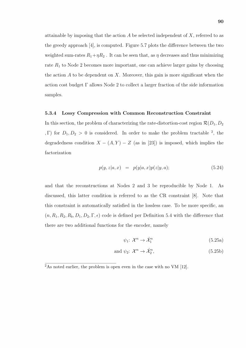
90
attainable by imposing that the action A be selected independent of X, referred to as
the greedy approach [4], is computed. Figure 5.7 plots the difference between the two
weighted sum-rates R1+ηR2 . It can be seen that, as η decreases and thus minimizing
rate R1 to Node 2 becomes more important, one can achieve larger gains by choosing
the action A to be dependent on X. Moreover, this gain is more significant when the
action cost budget Γ allows Node 2 to collect a larger fraction of the side information
samples.
5.3.4 Lossy Compression with Common Reconstruction Constraint
In this section, the problem of characterizing the rate-distortion-cost region R(D1, D2
,Γ) for D1, D2 > 0 is considered. In order to make the problem tractable 2, the
degradedness condition X − (A, Y ) − Z (as in [23]) is imposed, which implies the
factorization
p(y, z|a, x) = p(y|a, x)p(z|y, a); (5.24)
and that the reconstructions at Nodes 2 and 3 be reproducible by Node 1. As
discussed, this latter condition is referred to as the CR constraint [8]. Note that
this constraint is automatically satisfied in the lossless case. To be more specific, an
(n,R1, R2, Rb, D1, D2,Γ, ϵ) code is defined per Definition 5.4 with the difference that
there are two additional functions for the encoder, namely
ψ1: X n → X n1 (5.25a)
and ψ2: X n → X n2 , (5.25b)
2As noted earlier, the problem is open even in the case with no VM [12].

91
which map the source sequence into the estimated sequences at the encoder, namely
ψ1(Xn) and ψ2(X
n), respectively; and the CR requirements are imposed, i.e.,
Pr [ψ1(Xn) = h1(M1,Mb, Y
n)] ≤ ϵ (5.26a)
and Pr [ψ2(Xn) = h2(M2,Mb, Z
n)] ≤ ϵ, (5.26b)
so that the encoder’s estimates ψ1(·) and ψ2(·) are equal to the decoders’ estimates
(cf. (5.16)-(5.17)) with high probability.
Proposition 5.3. The rate-distortion region R(D1, D2,Γ) for the cascade-broadcast
source coding problem illustrated in Figure 5.4 under the CR constraint and the
degradedness condition (7.24) is given by the union of all rate triples (R1, R2, Rb)
that satisfy the conditions
Rb ≥ I(X;A) (5.27a)
R1 +Rb ≥ I(X;A) + I(X; X1, X2|A, Y ) (5.27b)
R2 +Rb ≥ I(X;A) + I(X; X2|A,Z) (5.27c)
and R1 +R2 +Rb ≥ I(X;A) + I(X; X2|A,Z) + I(X; X1|A, Y, X2), (5.27d)
where the mutual information terms are evaluated with respect to the joint pmf
p(x, y, z, a, x1, x2) = p(x)p(a|x)p(y|x, a)p(z|a, y)p(x1, x2|x, a), (5.28)
such that the inequalities
E[dj(X, Xj)] ≤ Dj, for j = 1, 2, (5.29a)
and E[Λ(A)] ≤ Γ, (5.29b)
are satisfied.

92
Remark 5.5. If either R1 = 0 or Rb = 0 and the side information Y is independent of
the action A given X, i.e., p(y|a, x) = p(y|x), the rate-distortion region R(D1, D2,Γ)
of Proposition 5.3 reduces to the one derived in [39, Proposition 10].
The proof of the converse is provided in Appendix N. The achievability follows
similar to Proposition 5.2. Specifically, Node 1 first maps sequence Xn into the action
sequence An. This mapping requires a codebook of rate I(X;A). This rate has to be
conveyed over link Rb by the definition of the problem and is thus received by both
Node 2 and Node 3. The source sequence Xn is mapped into the estimate Xn2 for
Node 3 using a codebook of rate I(X; X2|A) for each sequence An. Communicating
Xn2 to Node 2 requires rate I(X; X2|A, Y ) by the Wyner-Ziv theorem. This rate is
split into two rates r2b and r2d, such that the message corresponding to the first rate
is carried over the broadcast link of rate Rb and the second on the direct link of rate
R1. Note that Node 2 can thus recover sequence Xn2 . Communicating Xn
2 to Node
3 requires rate I(X; X2|A,Z) by the Wyner-Ziv theorem. This rate is split into two
rates r0b and r0d. The message corresponding to the rate r0b is send to Node 3 on
the broadcast link of the rate Rb by Node 1, while the message of rate r0d is sent by
Node 2 to Node 3. This way, Node 1 and Node 2 cooperate to transmit X2 to Node
3. Finally, the source sequence Xn is mapped by Node 1 into the estimate Xn1 for
Node 2 using a codebook of rate I(X; X1|A, X2) for each pair of sequences (An, Xn2 ).
Using the Wyner-Ziv coding, this rate is reduced to I(X; X1|A, Y, X2) and split into
two rates r1b and r1d, which are sent through links Rb and R1, respectively. As per
discussion above, the following inequalities have to be satisfied
r0b + r0d + r2b ≥ I(X; X2|A,Z),
r2b + r2d ≥ I(X; X2|A, Y ),

93
r1b + r1d ≥ I(X; X1|A, Y, X2),
R1 ≥ r1d + r2d,
R2 ≥ r0d,
and Rb ≥ r1b + r2b + r0b + I(X;A),
Applying Fourier-Motzkin elimination [1, Appendix C] to the inequalities above, the
inequalities in (5.27) are obtained.
5.4 Adaptive Actions
In this section, it is assume that actions taken by the nodes are not only a function
of the message M2 for the model of Figure 5.3 or Mb for the models of Figure 5.4
and Figure 5.5, respectively, but also a function of the past observed side information
samples. Following [26], this case is referred to as the one with adaptive actions. Note
that for the cascade-broadcast problem, the model in Figure 5.5 is considered, which
differs from the one in Figure 5.4 considered thus far in that the side information
Z is not available at Node 3. At this time, it appears to be problematic to define
adaptive actions in the presence of two nodes that observe different side information
sequences. For the cascade model in Figure 5.3, a (n,R1, R2, D1, D2,Γ) code is defined
per Definition 8.1 with the difference that the action encoder (8.2) is modified to be
ℓ: [1, 2nR2 ]×Z i−1 → A, (5.30)
which maps the message M2 and the past observed decoder side information
sequence Zi−1 into the ith symbol of the action sequence Ai. Moreover, for the
cascade-broadcast model of Figure 5.5, the “action” function (5.15) in Definition 5.4
is modified as
ℓ: [1, 2nRb ]× Y i−1 → A, (5.31)

94
which maps the messageMb and the past observed decoder side information sequence
Y i−1 into the ith symbol of the action sequence Ai.
Proposition 5.4. The rate-distortion-cost region R(D1, D2,Γ) for the cascade
source coding problem illustrated in Figure 5.3 with adaptive action-dependent side
information is given by the rate region described in Proposition 5.1.
Proposition 5.5. The rate-distortion-cost region R(D1, D2,Γ) for the cascade-
broadcast source coding problem under the CR illustrated in Figure 5.5 with adaptive
action-dependent side information is given by the region described in Proposition 5.3
by setting Z = ∅.
Remark 5.6. The results above show that enabling adaptive actions does not increase
the achievable rate-distortion-cost region. These results generalize the observations
in [26] for the point-to-point setting, wherein a similar conclusion is drawn.
To establish the propositions above, it is sufficient to prove the converse. The
proofs for Proposition 5.4 and Proposition 5.5 are given in Appendix M and N,
respectively.
5.5 Concluding Remarks
In an increasing number of applications, communication networks are expected to be
able to convey not only data, but also information about control for actuation over
multiple hops. In this chapter, a baseline communication model with three nodes
connected in a cascade with the possible presence of an additional broadcast link is
evaluated. The optimal trade-off between rate, distortion and cost is characterized
for actuation in a number of relevant cases of interest. In general, the results point
to the advantages of leveraging a joint representation of data and control information
in order to utilize in the most efficient way the available communication links.
Specifically, in all the considered models, a layered coding strategy, possibly coupled

95
with rate splitting, has been proved to be optimal. This strategy is such that the
base layer has the double role of guiding the actions of the downstream nodes and of
providing a coarse description of the source, similar to [4]. Moreover, it is shown that
this base compression layer should be designed in a way that depends on the network
topology and on the relative cost of activating the different links.

CHAPTER 6
TWO-WAY COMMUNICATION WITH ADAPTIVE DATA
ACQUISITION
6.1 Introduction
In computer networks and machine-to-machine links, communication is often inter-
active and serves a number of integrated functions, such as data exchange, query and
control. As an illustrative example, consider the set-up in Figure 6.1 in which the
terminals labeled Node 1 and Node 2 communicate on bidirectional links. Node 2
has access to a database or, more generally, is able to acquire information from the
environment, e.g., through sensors. As a result of the communication on the forward
link (Figure 6.1-(a)), Node 2 wishes to compute some functions Xn2 , e.g., a suitable
average, of the data Xn available at Node 1 and of the information it can retrieve from
the environment1. The latter is measured as Y n by Node 2 (Fig 6.1-(b)). The forward
link (Fig 6.1-(a)) is also used by Node 1 to query Node 2 with the aim of retrieving
some information Xn1 about Y n from the environment through the backward link (Fig
6.1-(c)).
As reviewed in Chapter 4 and Chapter 5, information acquisition from the
environment at Node 2 is generally expensive in terms of system resources, e.g., time,
bandwidth or energy. For instance, accessing a remote database as in Fig 6.1-(b)
requires interfacing with a server by following the appropriate protocol, and activating
sensors entails some energy expenditure. Therefore, data acquisition by Node 2 should
be performed efficiently by adapting to the informational requirements of Node 1 and
Node 2 , i.e., to the requirements on the calculation of Xn1 and Xn
2 , respectively.
1Integer n represents the dimension of the data.
96
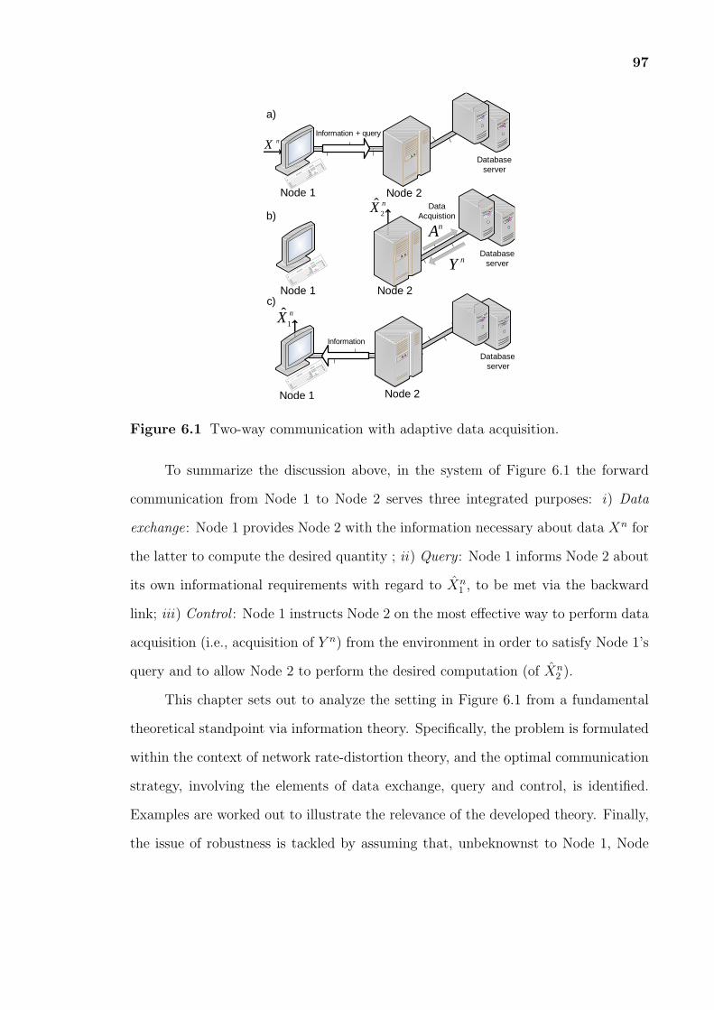
97
��������������������������������������������������������������������������������������������������������
Node 1 Node 2
Database server
����������������������������������������������������������������������������������������������������
Node 1 Node 2
Database server
����������������������������������������������������������������������������������������������������
����������������������������������������������������������������������������������������������������
Node 1 Node 2
Database server
Information + query
Data Acquistion
Information
nX
nA
nY
2ˆ nX
1ˆ nX
a)
b)
c)
Figure 6.1 Two-way communication with adaptive data acquisition.
To summarize the discussion above, in the system of Figure 6.1 the forward
communication from Node 1 to Node 2 serves three integrated purposes: i) Data
exchange: Node 1 provides Node 2 with the information necessary about data Xn for
the latter to compute the desired quantity ; ii) Query : Node 1 informs Node 2 about
its own informational requirements with regard to Xn1 , to be met via the backward
link; iii) Control : Node 1 instructs Node 2 on the most effective way to perform data
acquisition (i.e., acquisition of Y n) from the environment in order to satisfy Node 1’s
query and to allow Node 2 to perform the desired computation (of Xn2 ).
This chapter sets out to analyze the setting in Figure 6.1 from a fundamental
theoretical standpoint via information theory. Specifically, the problem is formulated
within the context of network rate-distortion theory, and the optimal communication
strategy, involving the elements of data exchange, query and control, is identified.
Examples are worked out to illustrate the relevance of the developed theory. Finally,
the issue of robustness is tackled by assuming that, unbeknownst to Node 1, Node

98
2 may be unable to acquire information from the environment, due to, e.g., energy
shortages or malfunctioning. The optimal robust strategy is derived and the examples
are extended to account for this generalized model. It should be mentioned that
the problem of characterizing the rate-distortion region for a two-way source coding
models, with conventional action-independent side information sequences at Node 2
has been addressed in [40, 41, 42] and references therein.
6.1.1 Contributions and Organization of the Chapter
This chapter studies the model in Figure 6.1, which is detailed in terms of a block
diagram in Figure 6.2. The system model is introduced in Section 6.2. The optimal
trade-off between the rates of the bidirectional communication, the distortions of
the reconstructions of the desired quantities at the two nodes, and the budget
for information acquisition at Node 2 is derived in Section 6.3. An example that
illustrates the application of the developed theory is discussed in Section 6.4. Finally,
in Section 6.5, the results are extended to the scenario in Figure 6.5 in which,
unbeknownst to Node 1, Node 2 may be unable to perform information acquisition.
Node 1
nX
nA
2X
( | , )p y a x
nY
Node 2
1M
nX
2M1X
Figure 6.2 Two-way source coding with a side information vending machine atNode 2.
6.2 System Model
The two-way source coding problem of interest, sketched in Figure 3.1, is formally
defined by the probability mass functions (pmfs) pX(x) and pY |A,X(y|a, x), and by
the discrete alphabets X ,Y ,A, X1, X2, along with distortion and cost metrics to

99
be discussed below. The source sequence Xn = (X1, ..., Xn) ∈ X n consists of n
independent and identically distributed (i.i.d.) entries Xi for i ∈ [1, n] with pmf
pX(x). Node 1 measures sequence Xn and encodes it in a message M1 of nR1 bits,
which is delivered to Node 2. Node 2 wishes to estimate a sequence Xn2 ∈ X n
2 within
given distortion requirements. To this end, Node 2 receives message M1 and based
on this, it selects an action sequence An, where An ∈ An.
The action sequence affects the quality of the measurement Y n of sequence Xn
obtained at Node 2. Specifically, given An and Xn, the sequence Y n is distributed
as p(yn|an, xn) =∏n
i=1 pY |A,X(yi|ai, xi). The cost of the action sequence is defined
by a cost function Λ: A →[0,Λmax] with 0 ≤ Λmax < ∞, as Λ(an) =∑n
i=1 Λ(ai).
The estimated sequence Xn2 with Xn
2 ∈ X n2 is then obtained as a function of M1 and
Y n. Upon reception on the forward link, Node 2 maps the message M1 received from
Node 1 and the locally available sequence Y n in a message M2 of nR2 bits, which is
delivered back to Node 1. Node 1 estimates a sequence Xn1 ∈ X n
1 as a function of M2
and Xn within given distortion requirements.
The quality of the estimated sequence Xnj is assessed in terms of the distortion
metrics dj(x, y, xj): X × Y × Xj → R+ ∪ {∞} for j = 1, 2, respectively. Note
that this implies that Xnj is allowed to be a lossy version of any function of the
source and side information sequences. A more general model is studied in Section
6.3.1. It is assumed that the distortion accrued in the absence of measurements and
communication is finite, i.e.,
Dj,max= minxj∈Xj
E[d(X, Y, Xj)] <∞ for j = 1, 2. (6.1)
A formal description of the operations at encoder and decoder follows.
Definition 6.1. An (n,R1, R2, D1, D2,Γ, ϵ) code for the set-up of Figure 3.1 consists
of a source encoder for Node 1
g1: X n → [1, 2nR1 ], (6.2)

100
which maps the sequence Xn into a message M1; an “action” function
ℓ: [1, 2nR1 ]× Y i−1 → A, (6.3)
which maps the messageM1 and the previously observed measurements into an action
sequence An; a source encoder for Node 2
g2: Yn × [1, 2nR1 ] → [1, 2nR2 ], (6.4)
which maps the sequence Y n and message M1 into a message M2; two decoders,
namely
h1: [1, 2nR2 ]×X n → X n
1 , (6.5)
which maps the message M2 and the sequence Xn into the estimated sequence Xn1 ;
h2: [1, 2nR1 ]× Yn → X n
2 , (6.6)
which maps the message M1 and the sequence Y n into the estimated sequence Xn2 ;
such that the action cost constraint Γ and distortion constraints Dj for j = 1, 2 are
satisfied, i.e.,
1
n
n∑i=1
E [Λ(Ai)] ≤ Γ (6.7)
and1
n
n∑i=1
E[dj(Xi, Yi, Xji)
]≤ Dj for j = 1, 2. (6.8)
Definition 6.2. Given a distortion-cost tuple (D1, D2,Γ), a rate tuple (R1, R2) is said
to be achievable if, for any ϵ > 0, and sufficiently large n, there exists a (n,R1, R2, D1+
ϵ,D2 + ϵ,Γ + ϵ) code.
Definition 6.3. The rate-distortion-cost region R(D1, D2,Γ) is defined as the
closure of all rate tuples (R1, R2) that are achievable given the distortion-cost tuple
(D1, D2,Γ).

101
Remark 6.1. For the special case in which the side information Y is independent of the
action A given X, i.e., for p(y|a, x) = p(y|x), the rate-distortion region R(D1, D2,Γ)
has been derived in [40]. Instead, if D1 = D1,max, the set of all achievable rates R1
was characterized in [4].
Remark 6.2. The definition (8.2) of an action encoder allows for adaptation of the
actions to the previously observed values of the side information Y . This possibility
was studied in [26] for the point-to-point one-way model, which is obtained by setting
R2 = 0 in the setting of Figure 3.1.
6.3 Rate-Distortion-Cost Region
In this section, a single-letter characterization of the rate-distortion-cost region is
derived.
Proposition 6.1. The rate-distortion-cost region R(D1, D2,Γ) for the two-way
source coding problem illustrated in Figure 3.1 is given by the union of all rate pairs
(R1, R2) that satisfy the conditions
R1 ≥ I(X;A) + I(X;U |A, Y ) (6.9a)
and R2 ≥ I(Y ;V |A,X,U), (6.9b)
where the mutual information terms are evaluated with respect to the joint pmf
p(x, y, a, u, v) = p(x)p(a, u|x)p(y|a, x)p(v|a, u, y), (6.10)
for some pmfs p(a, u|x) and p(v|a, u, y) such that the inequalities
E[d1(X,Y, f1(V,X))] ≤ D1, (6.11a)
E[d2(X,Y, f2(U,Y))] ≤ D2, (6.11b)
and E[Λ(A)] ≤ Γ, (6.11c)

102
are satisfied for some function f1: V × X → X1 and f2: U × Y → X2. Finally, U
and V are auxiliary random variables whose alphabet cardinality can be constrained
as |U| ≤ |X ||A|+ 4 and |V| ≤ |U||Y||A|+ 1 without loss of optimality.
Remark 6.3. For the special case in which the side information Y is independent of the
action A given X, i.e., for p(y|a, x) = p(y|x), the rate-distortion region R(D1, D2,Γ)
in Proposition 6.1 reduces to that derived in [40, 41]. Instead, if D1 = D1,max, the
result reduces to that in [4].
The proof of the converse is provided in Appendix O. The achievability follows
as a combination of the techniques proposed in [4] and [40], and requires the forward
link to be used, in an integrated manner, for data exchange, query and control.
Specifically, for the forward link, similar to [4] (see Chapter 2 and Figure 2.5), Node
1 uses a successive refinement codebook. Accordingly, the base layer is used by Node
1 to instruct Node 2 on which actions are best tailored to fulfill the informational
requirements of both Node 1 and Node 2. This base layer thus represents control
information that also serves the purpose of querying Node 2 in view of the backward
communication. Node 1 selects this base layer as a function of the source Xn,
thus allowing Node 2 to adapt its actions for information acquisition to the current
realization of the source Xn. The refinement layer of the code used by Node 1 is
leveraged, instead, to provide additional information to Node 2 in order to meet
Node 2’s distortion requirement. Node 2 then employs standard Wyner-Ziv coding
(i.e., binning) [1] for the backward link to satisfy Node 1’s distortion requirement.
The main technical aspects of the achievability proof is briefly outlined
here, since the details follow from standard arguments and do not require further
elaboration here. To be more precise and with reference to Figure 2.5, Node 1 first
maps sequence Xn into the action sequence An using the standard joint typicality
criterion. This mapping requires a codebook of rate I(X;A) (see, e.g., [1, pp. 62-63]).
Given the sequence An, the description of sequence Xn is further refined through

103
mapping to a sequence Un. This requires a codebook of size I(X;U |A, Y ) for each
action sequence An using Wyner-Ziv binning with respect to side information Y n [1,
pp. 62-63]. In the reverse link, Node 2 employs Wyner-Ziv coding for the sequence
Y n by leveraging the side information Xn available at Node 1 and conditioned on the
sequences Un and An, which are known to both Node 1 and Node 2 as a result of
the communication on the forward link. This requires a rate equal to the right-hand
side of (6.9b). Finally, Node 1 and Node 2 produce the estimates Xn1 and Xn
2 as
the symbol-by-symbol functions X1i = f1(Vi, Xi) and X2i = f2(Ui, Yi) for i ∈ [1, n],
respectively.
Remark 6.4. The achievability scheme discussed above uses actions that do not adapt
to the previous values of the side information Y . The fact that this scheme attains the
optimal performance characterized in Proposition 6.1 shows that, as demonstrated
in [26] for the one-way model with R2 = 0, adaptive actions do not improve the
rate-distortion performance.
6.3.1 Indirect Rate-Distortion-Cost Region
In this section, a more general model in which Node 1 observes only a noisy version
of the source Xn, as depicted in Figure 6.3 is considered. Following [43], this setting
is referred to as posing an indirect source coding problem. The example studied in
Section 6.4 illustrates the relevance of this generalization. The system model is as
defined in Section 6.2 with the following differences. The source encoder for Node 1
g1: Zn → [1, 2nR1 ], (6.12)
maps the sequence Zn into a message M1; the decoder for Node 1
h1: [1, 2nR2 ]×Zn → X n
1 , (6.13)

104
maps the message M2 and the sequence Zn into the estimated sequence Xn1 ;
given (Xn, An, Zn), the side information Y n is distributed as p(yn|an, xn, zn) =∏ni=1 pY |A,X,Z(yi|ai, xi, zi) and the distortion constraints are given as
1
n
n∑i=1
E[dj(Xi, Yi, Zi, Xji)
]≤ Dj for j = 1, 2, (6.14)
for some distortion metrics dj(x, y, z, xj) : X ×Y ×Z ×Xj → R+ ∪{∞}, for j = 1, 2.
The next proposition derives a single-letter characterization of the rate-distortion-cost
region.
Node 1
nX
nA
nX 2ˆ
( | , , )p y a x z
nY
Node 2
nX1ˆ
nX
nZ
( | )p z x
nZ
2M
1M
Figure 6.3 Indirect two-way source coding with a side information vending machineat Node 2.
Proposition 6.2. The rate-distortion-cost region R(D1, D2,Γ) for the indirect two-
way source coding problem illustrated in Figure 6.3 is given by the union of all rate
pairs (R1, R2) that satisfy the conditions
R1 ≥ I(Z;A) + I(Z;U |A, Y ) (6.15a)
and R2 ≥ I(Y ;V |A,Z, U), (6.15b)
where the mutual information terms are evaluated with respect to the joint pmf
p(x, y, z, a, u, v)=p(x, z)p(a,u|z)p(y|a,x,z)p(v|a,u,y), (6.16)

105
for some pmfs p(a, u|x) and p(v|a, u, y) such that the inequalities
E[d1(X,Y,Z, f1(V,Z))] ≤ D1, (6.17a)
E[d2(X,Y,Z, f2(U,Y))] ≤ D2, (6.17b)
and E[Λ(A)] ≤ Γ, (6.17c)
are satisfied for some function f1: V × Z → X1 and f2: U × Y → X2. Finally, U
and V are auxiliary random variables whose alphabet cardinality can be constrained
as |U| ≤ |Z||A|+ 3 and |V| ≤ |U||Y||A|+ 1 without loss of optimality.
The proof of the achievability and converse follows with slight modifications
from that of Proposition 6.1. Specifically, in the achievability the sequence Xn is
replaced by its noisy version, i.e., the sequence Zn, and the rest of the proof remains
essentially unchanged. The proof of the converse is provided in Appendix O.
6.4 Case Study and Numerical Results
In this section, an example is considered for the set-up in Figure 6.3 in order to
illustrate the main aspects of the problem and the relevance of the theoretical results
derived above. Consider a sensor network consisting of two sensors deployed to
monitor a given phenomenon of interest (i.e., the concentration of a given chemical).
Assume that the state of the observed phenomenon is described by a random source
X ∼ Bern(0.5) (e.g., X = 0 indicates a low concentration of the chemical and X = 1
a high concentration). Due to malfunctioning or environmental causes, at each time
i, Node 1 measures Xi with probability 1− ϵ, and reports instead an unusual event e
(referred to as ”erasure”) with probability ϵ. This implies that Zi = e with probability
ϵ, and Zi = Xi with probability 1− ϵ, for i ∈ [1, n].
Node 2 has the double purpose of monitoring the operation of Node 1 and of
assisting Node 1 in case of measurement failures (erasures). To this end, if necessary,
Node 2 can measure the phenomenon Xi by investing a unit of energy. This is

106
modelled by assuming that the vending machine at Node 2 operates as follows:
Y =
X for A = 1
ϕ for A = 0, (6.18)
with cost constraint Λ(a) = a, for a ∈ {0, 1}, where ϕ is a dummy symbol representing
the case in which no useful information is acquired by Node 2. This model implies
that a cost budget of Γ limits the average number of samples of the sequence Y that
can be measured by Node 2 to around nΓ given the constraint (8.5).
Node 1 wishes to reconstruct the source Xn, while Node 2 is interested in
recovering Zn in order to monitor the operation of Node 1. The distortion functions
are the Hamming metrics d1(x, x1) = 1{x =x1} and d2(z, x2) = 1{z =x2}. Therefore,
the maximum distortions (6.1) are easily seen to be given by D1,max = 0.5 and
D2,max = 1−max{ϵ, (1− ϵ)/2}.
To obtain analytical insight into the rate-distortion-cost region, in the following
on a number of special cases are considered.
6.4.1 D1 = D1,max and D2 = 0
Consider the distortion requirements D1 = D1,max and D2 = 0. As a result, Node 1
requires no backward communication from Node 2, while Node 2 wishes to recover Zn
losslessly. In the context of the example, here the only functionality of the network
is the monitoring of the operation of Node 1 by Node 2. For the given distortions,
the rate-cost region in Proposition 6.2 can be evaluated as
R1 ≥ H2(ϵ) + (1− ϵ− Γ)+ (6.19a)
and R2 ≥ 0, (6.19b)
for any cost budget Γ ≥ 0, where H2(α) = −αlog2α− (1−α)log2(1−α) is the binary
entropy function.

107
A formal proof of this result can be found in Appendix P. The rate region (6.19)
shows that, as the cost budget Γ for information acquisition increases, the required
rate R1 decreases down to the rate H2(ϵ) that is required to describe only the erasures
process En with Ei = 1{Zi=e}, i = 1, ..., n, losslessly to Node 2. This can be explained
by noting that the time-sharing strategy discussed next achieves region (6.19) and is
thus optimal.
In the time-sharing strategy, Node 1 describes the process En losslessly to
Node 2 with H2(ϵ) bits per symbol. In addition to En, in order to obtain a lossless
reconstruction of Zn, Node 2 needs to be informed about Zi = Xi for all i in which
Ei = 0. Note that, there are around n(1 − ϵ) such samples of Zi. Node 1 describes
Zi = Xi for n(1 − ϵ − Γ)+ of these samples, while the remaining nmin(Γ, 1 − ϵ) are
measured by Node 2 through the vending machine. Note that, in the strategy just
described, sequence En can be interpreted as control data that is used by Node 2 to
adapt its information acquisition process. An alternative strategy based directly on
Proposition 6.2 can be found in Appendix P.
Figure 6.4 illustrates the rate R1 in (6.19a) versus the cost budget Γ for ϵ = 0.2
(line with circles). The first observation is that for Γ = 0, since there is no side
information available at Node 2, R1 = H2(ϵ)+1− ϵ = 1.52, which is the rate required
to transmit the sequence Zn losslessly to Node 2. Moreover, as mentioned, as the
cost budget Γ increases, the rate R decreases down to the value H2(ϵ) = 0.72 needed
to describe only the sequence En. Finally, it is observed that if Γ ≥ 1 − ϵ = 0.8
no further improvement of the rate is possible since Node 2 only needs to measure a
fraction (1− ϵ) of values of Xn in order to recover Zn losslessly.
6.4.2 D1 = 0 and D2 = D2,max
Here, the dual case is considered in which Node 1 wishes to reconstruct sequence
Xn losslessly (D1 = 0), while Node 2 does not have any distortion requirements

108
(D2 = D2,max). In the context of the example, the network thus operates with the
aim of allowing Node 1 to measure the phenomenon of interest Xn reliably. As shown
in Appendix P, if Γ ≥ ϵ, the rate-cost region is given by the union of all rate pairs
(R1, R2) such that
R1 ≥ H2(ϵ)− ΓH( ϵΓ
)(6.20a)
and R2 ≥ ϵ. (6.20b)
Moreover, for Γ < ϵ, the region is empty as the lossless reconstruction of X at Node
1 is not feasible.
A proof of this result based on Proposition 6.2 can be found in Appendix P. In
the following, it is argued that a natural time-sharing strategy, akin to that used for
the case D1 = D1,max, D2 = 0 above, would be suboptimal, implying that the optimal
strategy requires a more sophisticated approach based on the successive refinement
code presented in Section 6.3.
A natural time-sharing strategy would be the following. Node 1 describes nη
samples of the erasure process En, for some 0 ≤ η ≤ 1, losslessly to Node 2, using
rate R1 = ηH2(ϵ). This information is used by Node 1 to query Node 2 about the
desired information. Specifically, Node 2 sets Ai = 1 if Ei = 1, thus observing around
nηϵ samples Yi = Xi from the vending machine. These samples are needed to fulfill
the distortion requirements of Node 1. For all the remaining n(1 − η) samples, for
which Node 2 does not have control information from Node 1, Node 2 sets Ai = 1,
thus acquiring all the side information samples. Again, this is necessary given Node
1’s requirements. Node 2 conveys losslessly the nηϵ samples Yi = Xi obtained when
Ei = 1, which requires ηϵ bits per sample, along with the n(1 − η) samples Yi in
the second set, which amount instead to (1− η)H(X|Z) bits per sample. Note that
the rate is H(X|Z) by the Slepian-Wolf theorem [1, Chapter 10], since Node 1 has
109
side information Zi for the second set of samples. Overall, R2 = ηϵ + (1 − η)ϵ = ϵ
bits/source symbol. This entails a cost budget of Γ = ηϵ+1− η, and thus η = (1−Γ)(1−ϵ)
.
Figure 6.4 compares the rate R1 as in (6.20a) (line with squared markers) with
the corresponding rate obtained via time-sharing (dashed line), for ϵ = 0.2. As seen,
in this second case the time-sharing strategy is strictly suboptimal (except for the two
extreme case of Γ = 0 and Γ = 1). Moreover, as discussed above, achieving D1 = 0
is impossible for Γ ≤ ϵ, since Node 2 must obtain the fraction ϵ of samples of Xn
that Node 1 fails to measure in order to guarantee lossless reconstruction at Node 1.
Finally, for Γ = 1, there is no need for Node 1 to send any information to Node 2, as
Node 2 is able to acquire the sequence Xn and send back to Node 1 on the backward
link (using rate R2 = ϵ by the Slepian-Wolf theorem).
0 0.1 0.2 0.3 0.4 0.5 0.6 0.7 0.8 0.9 10
0.2
0.4
0.6
0.8
1
1.2
1.4
1.6
Cost Γ
R 1
D1=D1,max, D2=0
D1=0, D2=D2,max(time-sharing)
D1=0, D2=0
D1=0, D2=D2,max
Figure 6.4 Rate R1 versus cost Γ for the examples in Section 6.4 with ϵ = 0.2.

110
6.4.3 D1 = D2 = 0
The case in which both nodes wish to achieve lossless reconstruction, i.e.,D1 = D2 = 0
is considered. In this case, in the context of the example, both measurement of Node
1 and monitoring at Node 2 are required to operate correctly. As seen in the previous
case, achieving D1 = 0 is not possible if Γ < ϵ and thus this is a fortiori true for
D1 = D2 = 0. For Γ ≥ ϵ, the rate-cost region is given by
R1 ≥ H2(ϵ) + (1− Γ) (6.21a)
and R2 ≥ ϵ, (6.21b)
as shown in Appendix P.
A time-sharing strategy that achieves (6.21) is as follows. Node 1 describes
the process En losslessly to Node 2 with H2(ϵ) bits per symbol. This information
serves the functions of query and control for Node 2. In order to satisfy its distortion
requirement, Node 2 now needs to be informed about Zi = Xi for all i in which
Ei = 0. Note that there are n(1 − ϵ) such samples of Zi. Node 1 describes Zi = Xi
for n(1− Γ) ≤ n(1− ϵ) of these samples, while the remaining n(Γ− ϵ) are measured
by Node 2 through the vending machine. Node 2 compresses losslessly the sequence
of around nϵ samples of Xi with i such that Ei = 1 which requires R2 = ϵ bits per
sample.
Figure 6.4 illustrates the rate R1 in (6.21a) versus the cost budget Γ for ϵ = 0.2
(line with triangular markers). As discussed above, achieving D1 = 0 is impossible
for Γ ≤ ϵ. Moreover, for Γ = 1 the performance of system is identical to that with
D1 = D1,max and D2 = 0, since in this case the informational requirements of both
Node 1 and Node 2 are satisfied if Node 1 conveys the locations of the erasures to
Node 2 (which requires rate R1 = H2(ϵ) = 0.72).

111
6.5 When the Side Information May Be Absent
In this section, the results of the previous section are generalized to the scenario
in Figure 6.5 in which, unbeknownst to Node 1, Node 2 may be unable to perform
information acquisition due, e.g., to energy shortage or malfunctioning. The setup of
the general model is illustrated in Figure 6.5.
6.5.1 System Model
The formal description of an (n,R1, R2, D1, D2, D3,Γ, ϵ) code for the set-up of Figure
6.5 is given as in Section 6.3.1 (which generalizes the model in Section 6.2) with the
addition of Node 3. This added node, which has no access to side information, models
the case in which the receiver is not able to acquire the side information due to, e.g.,
malfunctioning. Note that the same message M1 from Node 1 is received by both
Node 2 and Node 3. This captures the fact that the information about whether or
not the recipient is able to access the side information is not available to Node 1. The
model in Figure 6.5 is a generalization of the so called Heegard-Berger problem [3, 9].
Formally, Node 3 is defined by the decoding function
h3: [1, 2nR1 ] → X n
3 , (6.22)
which maps the message M1 into the estimated sequence Xn3 ; and the additional
distortion constraint
1
n
n∑i=1
E[d3(Xi, Yi, Zi, X3i)
]≤ D3. (6.23)
It is remarked that adding a link between Node 3 and Node 1 cannot improve
the system performance because Node 3 does not have access to any additional
information. Therefore, there is no advantage in having a backward link from Node 3
to Node 1 because the information available at Node 3 is a subset of the information
available at Node 1. Therefore, this link is not included in the model.

112
nA
nX 2ˆ
( | , , )p y a x z
nY
Node 2
nX
3ˆ nXNode 3
Node 1
nX
nX1ˆ
nZ( | )p z x
nZ
1M
2M
Figure 6.5 Indirect two-way source coding when the side information vendingmachine may be absent at the recipient of the message from Node 1.
6.5.2 Rate-Distortion-Cost Region
In this section, a single-letter characterization of the rate-distortion-cost region is
derived for the set-up in Figure 6.5.
Proposition 6.3. The rate-distortion-cost region R(D1, D2, D3,Γ) for the two-way
source coding problem illustrated in Figure 6.5 is given by the union of all rate pairs
(R1, R2) that satisfy the conditions
R1 ≥ I(Z;A) + I(Z; X3|A) + I(Z;U |A, Y, X3) (6.24a)
and R2 ≥ I(Y ;V |A,Z, U, X3), (6.24b)
where the mutual information terms are evaluated with respect to the joint pmf
p(x, y, z, a, u, v) = p(x, z)p(a, u, x3|z)p(y|a, x, z)p(v|a, u, y, x3), (6.25)
for some pmfs p(a, u, x3|z) and p(v|a, u, y) such that the inequalities
E[d1(X, Y, Z, f1(V, Z))] ≤ D1, (6.26a)
E[d2(X, Y, Z, f2(U, Y ))] ≤ D2, (6.26b)
E[d3(X,Y, Z, X3)] ≤ D3, (6.26c)
and E[Λ(A)] ≤ Γ, (6.26d)

113
are satisfied for some function f1: V × Z → X1 and f2: U × Y → X2. Finally, U
and V are auxiliary random variables whose alphabet cardinality can be constrained
as |U| ≤ |Z||A|+ 3 and |V| ≤ |U||Y||A|+ 1 without loss of optimality.
The proof of the converse is provided in Appendix Q. The achievable rate
(6.24a) can be interpreted as follows. Node 1 uses a successive refinement code with
three layers. The first layer is defined as for Section 6.3 and carries query and control
information. The second and third layers are designed as in the optimal Heegard-
Berger scheme [3]. Specifically, the second layer is destined to both Node 2 and Node
3, while the third layer targets only Node 2, which has enhanced decoding capabilities
due to the availability of side information.
To provide further details, as for Proposition 6.1, the encoder first maps
the input sequence Zn into an action sequence An so that the two sequences are
jointly typical, which requires I(Z;A) bits/source sample. Then, it maps Zn into
the estimate Xn3 for Node 3 using a conditional codebook with rate I(Z; X3|A).
Finally, it maps Zn into another sequence Un using the fact that Node 2 has the
action sequence An, the estimate Xn3 and the measurement Y n. Using conditional
codebooks (with respect to Xn3 and An) and from the Wyner-Ziv theorem, this
requires I(Z;U |A, Y, X3) bit/source sample (see Chapter 2 and Figure 2.5). As for
the rate (6.24b), Node 2 employs Wyner-Ziv coding for the sequence Y n by leveraging
the side information Zn available at Node 1 and conditioned on the sequences Un,
An and Xn3 , which are known to both Node 1 and Node 2 as a result of the forward
communication. This requires a rate equal to the right-hand side of (6.24b) (see
Chapter 2 and Figure 2.5). Finally, Node 1 and Node 2 produce the estimates Xn1
and Xn2 as the symbol-by-symbol functions X1i = f1(Vi, Zi) and X2i = f2(Ui, Yi) for
i ∈ [1, n], respectively.

114
0 1 *
0 0 1
1 0 1
E3X
∞∞
Table 6.1 Erasure Distortion for Reconstruction at Node 3.
6.5.3 Case Study and Numerical Results
In this section, the binary example of Section 6.4 is extended to the set-up in Figure
6.5. Specifically, the same setting as in Section 6.4 is considered, with the addition
of Node 3. For the latter, a ternary reconstruction alphabet X3 = {0, 1, ∗} and
the distortion metric d3(x, z, x3) = d3(1{Z=e}, x3) in Table 6.1 are assumed, where
Ei = 1{Zi=e} is the erasure process2. Accordingly, Node 3 is interested in recovering
the erasure process En under an erasure distortion metric (see, e.g., [20]) , where “*”
represents the “don’t care” or erasure reproduction symbol
It is first observed that for cases 1) and 3) in Section 6.4 the distortion
requirements of Node 3 do not change the rate-distortion function. This is because,
as discussed in Section 6.4, the requirement that D2 be equal to zero entails that
the erasure process En be communicated losslessly to Node 2 without leveraging
the side information from the vending machine (which cannot provide information
about the erasure process). It follows that one can achieve D3 = 0 at no additional
rate cost. Therefore, let’s focus on the case 2) in Section 6.4, namely D1 = 0 and
D2 = D2,max = 1−max{ϵ, (1− ϵ)/2}.
In the case at hand, Node 1 wishes to recover Xn losslessly, Node 2 has no
distortion requirements and Node 3 wants to recover En with distortion D3. As
explained in Section 6.4.2, in order to reconstruct Xn losslessly at Node 1 Γ ≥ ϵ and
Pr(A = 1|Z = e) = 1 have to be satisfied. Moreover, due to symmetry of the problem
2Infinity in Table 1 means that the corresponding reconstruction is unacceptable at thedecoder and is thus measured to be infinity. This is a standard approach to account forerrors that are not allowed by design.

115
with respect to Z = 0 and Z = 1, one can set Pr(A = 1|Z = 0) = Pr(A = 1|Z =
1) = γ−ϵ1−ϵ
, for some 0 ≤ γ ≤ Γ. To evaluate the rate-distortion-cost region (6.24),
let’s define Pr(X3 = ∗|A = 1, Z = e)△= p1, Pr(X3 = ∗|A = 0, Z = 0)
△= p2 and
Pr(X3 = ∗|A = 1, Z = 0)△= p3. Thus, the rate-distortion-cost region is given by
R1 ≥ H2(ϵ) + 1− ϵ− (1− Γ)(1− p2)− (Γ− ϵ)
(1− p3)− (1− Γ)p2 −(ϵp1 + (Γ− ϵ)p3
)(H2(
ϵp1ϵp1 + (Γ− ϵ)p3
) +(Γ− ϵ)p3
ϵp1 + (Γ− ϵ)p3
)(6.27a)
and R2 ≥ ϵ, (6.27b)
where parameters p1, p2, p3 ∈ [0, 1] must be selected so as to satisfy the distortion
constraint of Node 3, namely D3 ≥ ϵp1 + (1− Γ)p2 + (Γ− ϵ)p3.
Figure 6.6 illustrates the rate R1 in (6.27a), minimized over p1, p2 and p3 under
the constraints mentioned above versus the cost budget Γ for ϵ = 0.2 and different
values of D3, namely D3 = 0.4, 0.6, 0.8 and D3 = D3,max = 1. Note that for
D3 = D3,max = 1 the rate in (6.20a) is obtained. As it can be seen, for Γ ≤ D3, the
rate decreases with increasing cost Γ, but for Γ ≥D3 the rate remains constant while
increasing Γ. The reason is that for the latter region, i.e., Γ ≥ D3, the performance of
the system is dominated by the distortion requirement of Node 3 and thus increasing
the cost budget Γ does not improve the rate. Instead, for Γ ≤ D3, it is sufficient to
cater only to Node 2, and Node 3 is able to recover E with distortion D3 = Γ at no
additional rate cost.
6.6 Concluding Remarks
For applications such as complex communication networks for cloud computing
or machine-to-machine communication, the bits exchanged by two parties serve a
number of integrated functions, including data transmission, control and query.

116
0.2 0.3 0.4 0.5 0.6 0.7 0.8 0.9 10
0.1
0.2
0.3
0.4
0.5
0.6
0.7
0.8
Cost Γ
R1
D3=0.4
D3=0.6
D3=0.8
D3=D
3,max=1
Figure 6.6 Rate R1 versus cost Γ for the examples in Section 6.5.3 with ϵ = 0.2,D1 = 0 and D2 = D2,max.
In this chapter, a baseline two-way communication scenario that captures some of
these aspects have been considered. The problem is addressed from a fundamental
theoretical standpoint using an information theoretic formulation. The analysis
reveals the structure of optimal communication strategies and can be applied to
elaborate on specific examples, as illustrated in this chapter. This work opens a
number of possible avenues for future research, including the analysis of scenarios
in which more than one round of interactive communication is possible, set-ups in
which there are multiple sources communicating to a single receiver in an interactive
fashion, or, dually, multiple receivers, each connected to its own vending machine.

CHAPTER 7
ON CHANNELS WITH ACTION-DEPENDENT STATES
7.1 Introduction
In [44], the framework of action-dependent channels was introduced as a means to
model scenarios in which transmission takes place in two successive phases. In the first
phase, the encoder selects an “action” sequence, with the twofold aim of conveying
information to the receiver and of affecting in a desired way the state of the channel
to be used in the second phase. In the second phase, communication takes place in
the presence the mentioned action-dependent state. With a cost constraint on the
actions in the first phase and on the channel input in the second phase, reference
[44] derived the capacity-cost-trade-off under the assumption that the channel state
is available either causally or non-causally at the encoder in the second phase.
A number of applications and extensions of the results in [44] have been reported
since then. In [45], the result in [44] is leveraged to study a model in which encoder
and decoder can “probe” the channel state to obtain partial state information during
the first communication phase. In [46], unlike [44] the decoder is required to decode
both the transmitted message and channel input reliably. Finally, in [47], the decoder
is interested in estimating not only the message but also the state sequence, and the
latter is available strictly causally at the encoder in the second transmission phase.
In this chapter, two further extensions of the original action-dependent channel
are studied. In the first, similar to [47], the decoder is interested in estimating not
only the message but also the state sequence within given average per-letter distortion
constraints (see Figure 7.1). Unlike [47], it is assumed non-causal state knowledge
in the second phase, and, under the constraint of common reconstruction (CR) (i.e.,
the decoder’s estimate of the state must be recoverable also at the encoder with high
117

118
probability [8]), a single-letter characterization of the achievable rate-distortion-cost
trade-off is obtained. It is remarked that, for conventional state-dependent states
without actions, the problem of joint estimation of message and state with non-causal
state information at the encoder without the CR constraint is open (see, e.g., [48]),
while with the CR constraint the problem has been solved in [8]. In the second
extension, illustrated in Figure 7.2, an action-dependent degraded broadcast channel
is studied. Under the assumption that the encoder knows the state sequence causally
in the second phase, the capacity-cost region is identified.1 The corresponding result
for action-independent states was derived in [51] (see also [52]), while it is recalled that
with non-causal state information the problem is open (see [53]). Various examples,
including Gaussian channels and a model with a ”probing” encoder, are also provided
throughout to show the advantage of a proper joint design of the two communication
phases.
Channel Encoder
nXnSM ˆ,ˆ
Decoder
Action Encoder
M nA )|( asp
),,|( asxyp
nS
nY
ψ )( nSψ.
Figure 7.1 Channel with action-dependent state in which the decoder estimatesboth message and state, and there is a a common reconstruction (CR) constraint onthe state reconstruction. The state is known non-causally at the channel encoder.
7.2 Transmission of Data and Action-Dependent State with Common
Reconstruction Constraint
In this section, the setting illustrated in Figure 7.1 of a channel with action-dependent
state is studied in which the decoder estimates both message and state. First, the
1After submitting [49], the authors are informed of the reference [50], where the problemillustrated in Figure 7.2 has also been solved.

119
system model is detailed in Section 8.4.1. Next, the characterization of the trade-off
between the achievable data rate and state reconstruction distortion is derived in
Section 8.4.2. Finally, a Gaussian example is given in Section 7.2.3.
Channel Encoder
iX
1MDecoder 1
Action Encoder
21,MMiA
)|( asp
),,|,( 21 asxyyp
iS
2MDecoder 2
iY2
iY1
Figure 7.2 Broadcast channel with action-dependent states known causally to theencoder (i.e., the ith transmitted symbol Xi is a function of messages M1, M2 andthe state symbols up to time i, Si).
7.2.1 System Model
In this section, the system model is detailed. The system is defined by the
probability mass functions (pmfs) p(x), p(y|x, s, a), p(s|a) and discrete alphabets
X ,A, S, S, and Y as follows. Given the message M , selected randomly from the set
M = [1, 2nR], an action sequence An ∈ An is selected. As a result of this selection,
the state sequence Sn ∈ Sn is generated as the output of a memoryless channel p(s|a)
so that p(sn|an) =∏n
i=1 p(si|ai) holds for an action sequence An = an. The input
sequence Xn ∈ X n is selected based on both message M and state sequence Sn. The
action sequence An and the inputXn have to satisfy an average cost constraint defined
by a function γ : A×X → [0,∞), so that the cost for the input sequences an and xn
is given by γ(an, xn) = 1n
∑ni=1 γ(ai, xi). Given Xn = xn, Sn = sn and An = an, the
received signal is distributed as p(yn|xn, sn, an) =∏n
i=1 p(yi|xi, si, ai). The decoder,
based on the received signal Y n, estimates the messageM and the sequences Sn ∈ Sn.
The estimate Sn ∈ Sn is constrained to satisfy a distortion criterion defined by a
per-symbol distortion metric d(s, s) : S × S → [0, Dmax] with 0 < Dmax < ∞.
Based on the given distortion metric, the overall distortion for the estimated state

120
sequences sn is defined as dn(sn, sn) = 1n
∑ni=1 d(si, si). The reconstructions S
n is also
required to satisfy the CR constraint, which imposes that the state estimate be also
reproducible at the encoder with high probability, as formalized below.
Definition 7.1. An (n,R,D,Γ, ϵ) code for the model in Figure 7.1 consists of an
action encoder
g1: M → An, (7.1)
which maps message M into an action sequence An; a channel encoder
g2: M×Sn → X n, (7.2)
which maps messageM and the state sequence Sn into the sequenceXn; two decoding
functions,
h1: Yn → M, (7.3)
and h2: Yn → Sn, (7.4)
which map the sequence Y n1 into the estimated message M and into the estimated
sequence Sn, respectively; and a reconstruction function
ψ: Sn → Sn, (7.5)
which maps the state sequence into the estimated state sequence at the encoder; such
that the probability of error in decoding the message M is small
Pr[M =M ] ≤ ϵ, (7.6)

121
the distortion and cost constraints are satisfied, i.e.,
1
n
n∑i=1
E [d(Si, h2i(Yn))] ≤ D + ϵ (7.7)
and1
n
n∑i=1
E [γ(Ai, Xi)] ≤ Γ + ϵ, (7.8)
where h2i(Yn) ∈ S is the ith symbol of the sequence h2(Y
n), and the CR requirement
is verified, namely,
Pr [ψ(Sn) = h2(Yn)] ≤ ϵ. (7.9)
It is noted that, given the definition above, the pmf of the random variables (M,An, Sn
, Xn, Y n) factorizes as
p(m, an, sn, xn, yn) =1
2nRδ[an − g1(m)]
{n∏
i=1
p(si|ai)
}δ[xn − g2(m, s
n)]
·
{n∏
i=1
p(yi|xi, si, ai)
}, (7.10)
where δ[·] is the Kronecker delta function (i.e., δ[x] = 1 if x = 0 and δ[x] = 0
otherwise) and the arguments of the pmf range in the alphabets of the corresponding
random variables.
Given a cost-distortion pair (D,Γ), a rate R is said to be achievable if, for
any ϵ > 0 and sufficiently large n, there a exists a (n,R,D,Γ, ϵ) code. The goal is
to characterize the capacity-distortion-cost trade-off function C(D,Γ) =inf{R : the
triple (R,D,Γ) is achievable}.
7.2.2 Capacity-Distortion-Cost Function
In this section, a single-letter characterization of the capacity-distortion-cost function
is derived.

122
Proposition 7.1. The capacity-distortion-cost function for the system in Figure 7.1
is given by
C(D,Γ) = max I(U ;Y )− I(U ;S|A) (7.11)
where the mutual informations are evaluated with respect to the joint pmf
p(a, u, s, x, y) = p(a)p(s|a)p(u|s, a)p(x|u, s)p(y|x, s, a), (7.12)
and minimization is done with respect to the pmfs p(a), p(u|s, a) and p(x|u, s) under
the constraint that there exists a deterministic function ϕ : U → S such that the
inequalities
E[d(S, ϕ(U))] ≤ D (7.13a)
and E[γ(A,X)] ≤ Γ (7.13b)
are satisfied. Finally, U is an auxiliary random variable whose alphabet cardinality
can be bounded as |U| ≤ |A||S||X |+ 2.
Remark 7.1. If D ≥ Dmax, the result above recovers Theorem 1 of [44]. If instead,
p(s|a) = p(s), so that the channel is not action-dependent, Theorem 1 in [8] is
recovered.
The proof of achievability follows using the same arguments as in [44] with the
difference that here U is also used to estimate the state S via a function ϕ(U). The
proof of the converse can be found in Appendix R.
7.2.3 A Gaussian Example
In this section, a continous-alphabet version of the model of Figure 7.1 is considered
in which the actions and the channel input are subject to the cost constraints
1/n∑n
i=1 E[A2] ≤ PA and 1
n
∑ni=1 E [X2
i ] ≤ PX , respectively; the action channel is

123
given by
S = A+W, (7.14)
where W ∼ N (0, σ2W ) and the transmission channel is given by
Y = X + S + Z, (7.15)
where Z ∼ N (0, σ2Z) is independent of W . The rate I(U ;Y ) − I(U ;S|A) in (7.11)
is evaluated by assuming the variables (A, S, U,X, Y ) to be jointly Gaussian without
claiming the optimality of this choice. Specifically, similar to [44, Section VI], let’s
choose A ∼ N (0, PA),
X = αA+ γW +G (7.16a)
and U = δX + A+ βW, (7.16b)
with G ∼ N (0, PX − (α2PA + γ2σ2W )), where the constraint PX ≥ (α2PA + γ2σ2
W ) is
enforced, and the variables (A,W,G,Z) are all independent of each other. Then the
rate I(U ;Y )−I(U ;S|A) as in [44] is evaluated, with the additional constraint (7.7) on
the state estimate S. Assuming the quadratic distortion metric d(s, s) = (s− s)2, S
is chosen to be the MMSE estimate of S given U and A.2 This leads to the constraint
D ≥ E[(S − S)2] = var(S|U,A) = σ2W − (E[W (U − A)])2
E[(U − A)2], (7.17)
where E[W (U − A)] = (δγ + β)σ2W and E[(U − A)2] = δ2PG + (δγ + β)2σ2
W . The
rate I(U ;Y )− I(U ;S|A) optimized over parameters (α, β, δ, γ) under the constraint
(7.17) for different values of the distortion D for PA = PX = σ2W = σ2
Z = 1 in Figure
(7.3). Moreover for reference, Figure 7.3 shows also the rate achievable if distribution
(8.8) is designed to be optimal for message transmission only as in [44, eq. (95)],
2Note that U in the characterization of Proposition 2 can be always redefined to includealso A without loss of performance, and hence S can be made to be a function of U and A.

124
and the rate achievable, if A is selected to be independent of the message, namely,
max I(U ;Y |A)− I(U ;S|A), where the mutual information terms are evaluated with
respect to the joint Gaussian distribution given above in (7.16) under the constraint
(7.17). The performance gains attainable by designing the transmission strategy
jointly in the two phases and by accounting for the constraint (7.17) are apparent.
0 0.1 0.2 0.3 0.4 0.5 0.6 0.7 0.8 0.9 10
0.1
0.2
0.3
0.4
0.5
0.6
Distortion D
Rat
e [n
ats/
chan
nel
use]
Actions selected for message transmission onlyActions selected based on messageActions selected independent of the message
Figure 7.3 Achievable rates (constrained to a Gaussian joint distribution, see(7.16)) for the Gaussian model (7.14)-(7.15) versus distortion D for PA = PX =σ2W = σ2
Z = 1.
7.3 Degraded Broadcast Channels with Action-Dependent States
In this section, the problem illustrated in Figure 7.2 of a broadcast channel with
action-dependent states known causally to the encoder is studied. First, the system
model is detailed in Section 7.3.1. Next, the characterization of the capacity region
for physically degraded broadcast channels is given in Section 7.3.2. In Section 7.3.4,

125
the special case of a broadcast channel with a probing encoder in the sense of [45] is
studied.
7.3.1 System Model
In this section, the system model is detailed. The system is defined by the pmfs p(x),
p(y1, y2|x, s, a), p(s|a) and discrete alphabets X , A, S, and Y as follows. Given the
messages M1 and M2, selected randomly from the sets M1 = [1, 2nR1 ] and M2 =
[1, 2nR2 ], respectively, an action sequence An ∈ An is selected. As a result of this
selection, the state sequence Sn ∈ Sn is generated as in the previous section. The
action sequence An and the input Xn have to satisfy the average cost constraint
(8.38). Given the transmitted signal Xn = xn, the state sequence Sn = sn, and the
action sequence An = an, the received signals are distributed as p(yn1 , yn2 |xn, sn, an) =∏n
i=1 p(y1i, y2i|xi, si, ai). The decoders, based on the received signals Y n1 and Y n
2 ,
estimate the messages M1 and M2, respectively.
Definition 7.2. An (n,R1, R2,Γ, ϵ) code for the model in Figure 7.2 consists of an
action encoder
g1: M1 ×M2 → An, (7.18)
which maps messages M1 and M2 into an action sequence An; a sequence of channel
encoders
g2i: M1 ×M2 × S i → X , (7.19)
for i ∈ [1, n] which map messages M1 and M2 and the first i samples of the state
sequence Si into the ith symbol Xi; two decoding functions,
h1: Yn1 → M1, (7.20)
and h2: Yn2 → M2, (7.21)
126
which map the received sequences Y n1 and Y n
2 into the estimated messages M1 and
M2, respectively; such that the probability of error in decoding the messages M1 and
M2 is small
Pr[Mj =Mj] ≤ ϵ for j = 1, 2, (7.22)
and the cost constraint (8.38) is satisfied.
It is noted that, given the definitions above, the distribution of the random
variables (M1,M2, An, Sn, Xn, Y n
1 , Yn2 ) factorizes as
p(m1,m2, an, sn, xn, yn1 , y
n2 ) =
1
2n(R1+R2)δ[an − g1(m1,m2)] ·
{n∏
i=1
p(si|ai)δ[xi − g2i(m1,m2, si)]p(y1i, y2i|xi, si, ai)
},
(7.23)
where the arguments of the pmf range in the alphabets of the corresponding random
variables.
Given a cost Γ, a rate pair (R1, R2) is said to be achievable if, for any ϵ > 0 and
sufficiently large n, there a exists a (n,R1, R2,Γ, ϵ) code. The capacity region C(Γ) is
defined as the closure of all rate pairs (R1, R2) that are achievable given the cost Γ.
7.3.2 Capacity-Cost Region
In this section, a single-letter characterization of the capacity region is derived for
the special case in which the channel is physically degraded in the sense that the
condition below is satisfied
p(y1, y2|x, s, a) = p(y1|x, s, a)p(y2|y1), (7.24)
or equivalently, the Markov chain (Xi, Si, Ai)− Y1i − Y2i holds for all i ∈ [1, n].

127
Proposition 7.2. The capacity region of the system in Figure 7.2 under the
degradedness condition (7.24) is given by the union of the rate pairs (R1, R2) satisfying
R1 ≤ I(U1;Y1|U2) (7.25a)
and R2 ≤ I(U2;Y2), (7.25b)
where the mutual informations are evaluated with respect to the joint pmf
p(a, u1, u2, s, x, y1, y2) = p(u1, u2)
· δ[a− fa(u1, u2)]p(s|a)δ[x− fx(u1, u2, s)]p(y1|x, s, a)p(y2|y1), (7.26)
for some pmfs p(u1, u2) and deterministic functions fa: U1 × U2 → A and fx: U1 ×
U2 × S → X such that the inequality E[γ(A,X)] ≤ Γ is satisfied. Auxiliary random
variables U1 and U2 have finite alphabets.
The proof of achievability can be sketched as follows. The codewords
un2 (m2), encoding message m2 ∈ [1, 2nR2 ], are generated independently and i.i.d.
according to the pmf p(u2). Then, superimposed on each codeword un2 (m2), 2nR1
codewords un1 (m1,m2) are generated independently according to the distribution∏ni=1 p(u1i|u2i(m2)). To encode messages (M1,M2), the action sequence An is
obtained as a deterministic function of u1i(M1,M2) and u2i(M2) such that Ai =
fa(u1i(M1,M2), u2i(M2)) for all i ∈ [1, n]. The transmitted symbol Xi is obtained
instead as a function of u1i(M1,M2), u2i(M2), and of the ith state symbol Si
as Xi = fx(u1i(M1,M2), u2i(M2), Si). Decoder 2 decodes the codeword un2 (m2),
while decoder 1 decodes both codewords un2 (m2) and un1 (m1,m2). Using standard
arguments, the rates (7.25) are easily shown to be achievable. The proof of the
converse can be found in Appendix S.
Remark 7.2. If p(s|a) = p(s) so that the channel is not action-dependent, Proposition
6 recovers Proposition 4 of [51] (see also [52]).

128
7.3.3 A Binary Example
In this section, let’s consider a special case of the model in Figure 7.2 in which the
action channel p(s|a) is binary and given by
S = A⊕B, (7.27)
where the action A is binary, B ∼ Ber(b) and the transmission channels are given by
Y1 = X ⊕ S ⊕ Z1, (7.28a)
and Y2 = Y1 ⊕ Z2, (7.28b)
where Z1 ∼ Ber(N1) and Z2 ∼ Ber(N2) are independent of each other and of B. The
cost metric is selected as γ(a, x) = x. Moreover, N2 = N1 ∗ N2 = N1(1− N2)+ N2(1−
N1).
As a first remark, consider the ideal system with b = 0 (i.e., no interference)
and no cost constraint (i.e., Γ = 1/2). The system reduces to a standard physical
degraded binary symmetric broadcast channel, and thus the capacity region is given
by the union over α ∈ [0, 0.5] of the rate pairs satisfying the inequalities [1, p. 115]
R1 ≤ H(α ∗N1)−H(N1) (7.29a)
and R2 ≤ 1−H(α ∗N2). (7.29b)
It is observed that, by construction, this rate region sets an outer bound on the
rate achievable in the system at hand. The outer bound above is in fact achievable by
setting X = B, U2 ∼ Ber(1/2), U1 = U2⊕ U1 with U1 ∼ Ber(α), and A = U1 in (7.25),
where U2 and U1 are independent. This entails that, by leveraging the actions, the
interference-free capacity region (7.29) is obtained for all cost constraints Γ ≥ b. It
can be instead seen that, if one is forced to set A to be constant, achieving the rate
region (7.29) requires a cost Γ = 1/2, since X needs to be distributed Ber(1/2). This

129
example illustrates the advantage of being able to affect the state via actions selected
as a function of the messages.
7.3.4 Probing Capacity of Degraded Broadcast Channels
In this section, the setting of probing capacity introduced in [45] is applied to the
degraded broadcast channel. Following [45], the state sequence Sn is thus assumed
to be generated i.i.d. according to a pmf p(s). Moreover, based on the messages
(M1,M2), the encoder selects an action sequence as in (7.18). However, here, through
the choice of actions, the encoder affects the state information available at the encoder
and the decoders, and not the state sequence Sn. Specifically, the encoder obtains
partial state information Se,i = be(Si, Ai), and the decoders obtain partial state
informations Sd1,i = bd1(Si, Ai) and Sd2,i = bd2(Sd1,i), respectively, where i ∈ [1, n], and
be : S×A → Se, bd1 : S×A → Sd1 and bd2 : Sd1 → Sd2 are deterministic functions for
given alphabets Se, Sd1 and Sd2 . Note that the state information available at decoder
2 is degraded with respect to that of decoder 1 (i.e., it is a function of the latter). As
in [45], it is assumed that the state information at the encoder is characterized as
Se,i = be(Si, Ai) =
Si if Ai = 1
∗ if Ai = 0
, (7.30)
where ∗ represents the absence of channel state information at the encoder. Moreover,
the state information Se,i is assumed to be available causally at the encoder so that
the encoding function is g2i: M1 ×M2 × S ie → X (cf. (7.19)). The rest of the code
definition is similar to Definition 7.2 with the caveat that the decoder 1 and 2 have
available also the information sequences Snd1
and Snd2, respectively.

130
It is noted that, given the definitions above, the distribution of the random
variables (M1,M2, An, Sn, Xn, Y n
1 , Yn2 ) factorizes as
p(m1,m2, an, sn, sne , s
nd1, snd2 , x
n, yn1 , yn2 ) =
1
2n(R1+R2)δ[an − g1(m1,m2)]
·
{n∏
i=1
p(si)δ[se,i − be(si, ai)]δ[sd1,i − bd1(si, ai)]δ[xi − g2(m1,m2, sie)
}
·
{n∏
i=1
δ[sd2,i − bd2(sd1,i)]p(y1i, y2i|xi, si, ai)
}(7.31)
where the arguments of the pmf range in the alphabets of the corresponding random
variables.
As discussed below, the setting at hand, which is referred to as having a probing
encoder, is a special case of the one studied in Section 8.4.1. Therefore, one can
leverage Proposition 7.2 to obtain the following result.
Proposition 7.3. The capacity region of the system in Figure 7.2 under the
degradedness condition (7.24) and with a probing encoder is given by the union of
the rate pairs (R1, R2) satisfying
R1 ≤ I(U1;Y1, Sd1 |U2) (7.32a)
and R2 ≤ I(U2;Y2, Sd2) (7.32b)
where the mutual informations are evaluated with respect to the joint pmf
p(a, u1, u2, s, se, sd1 , sd2 , x, y1, y2) = p(s)p(u1, u2)
δ[a− fa(u1, u2)]δ[se − be(s, a)] · δ[sd1 − bd1(s, a)]
δ[sd2 − bd2(sd1)] · δ[x− fx(u1, u2, se)]p(y1|x, s, a)p(y2|y1), (7.33)
for some pmf p(u1, u2) and deterministic functions fa: U1 × U2 → A and fx: U1 ×
U2 × Se → X such that the inequality E [γ(A,X)] ≤ Γ is satisfied.

131
Proof. The result is obtained by noticing that the setting described above is a special
case of the one described in Section 7.3.1 by making the following substitutions
S → Se (7.34a)
and Yj → (Yj, Sdj) for j = 1, 2. (7.34b)
To see this, it will be shown that the pmf (7.31) reduces to (7.23) under the given
substitutions. Specifically, by marginalizing (7.31) over Sn it is true that
1
2n(R1+R2)δ[an − g1(m1,m2)]
{n∏
i=1
δ[xi − g2(m1,m2, sie)]δ[sd2,i − bd2(sd1,i)]p(y2i|y1i)
}n∏
i=1
∑si∈S
{p(si)δ[se,i − be(si, ai)]δ[sd1,i − bd1(si, ai)]p(y1i|xi, si, ai)
}.(7.35)
The terms outside the summation in (7.35) are equal to the corresponding terms in
(7.23) under the substitutions (7.34). For the remaining terms, it is observed that,
for ai = 0, Se,i = ∗, and thus p(se,i|ai) = δ[se,i − ∗] and
p(y1i, sd1i|xi, se,i, ai) =∑si∈S
p(si)δ[sd1,i − bd1(si, ai)]p(y1i|xi, si, ai);
instead, for ai = 1, Se,i = Si, and thus p(se,i|ai) = Pr[Si = se,i] and
p(y1i, sd1i|xi, se,i, ai) = δ[sd1,i − bd1(se,i, ai)]p(y1i|xi, se,i, ai),
which completes the proof.
7.4 Concluding Remarks
Action-dependent channels are useful abstractions of two-phase communication
scenarios. This chapter has reported on two variations on this theme, namely the
problem of message and state transmission in an action-dependent channel and
the degraded action-dependent broadcast channel. Under given assumptions, the
information-theoretic performance of these systems is characterized. The analytical

132
results, and specific examples, emphasize the importance of jointly designing the
transmission strategy across the two communication phases.
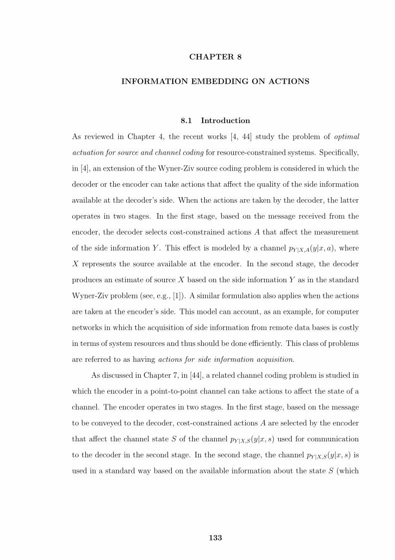
CHAPTER 8
INFORMATION EMBEDDING ON ACTIONS
8.1 Introduction
As reviewed in Chapter 4, the recent works [4, 44] study the problem of optimal
actuation for source and channel coding for resource-constrained systems. Specifically,
in [4], an extension of the Wyner-Ziv source coding problem is considered in which the
decoder or the encoder can take actions that affect the quality of the side information
available at the decoder’s side. When the actions are taken by the decoder, the latter
operates in two stages. In the first stage, based on the message received from the
encoder, the decoder selects cost-constrained actions A that affect the measurement
of the side information Y . This effect is modeled by a channel pY |X,A(y|x, a), where
X represents the source available at the encoder. In the second stage, the decoder
produces an estimate of source X based on the side information Y as in the standard
Wyner-Ziv problem (see, e.g., [1]). A similar formulation also applies when the actions
are taken at the encoder’s side. This model can account, as an example, for computer
networks in which the acquisition of side information from remote data bases is costly
in terms of system resources and thus should be done efficiently. This class of problems
are referred to as having actions for side information acquisition.
As discussed in Chapter 7, in [44], a related channel coding problem is studied in
which the encoder in a point-to-point channel can take actions to affect the state of a
channel. The encoder operates in two stages. In the first stage, based on the message
to be conveyed to the decoder, cost-constrained actions A are selected by the encoder
that affect the channel state S of the channel pY |X,S(y|x, s) used for communication
to the decoder in the second stage. In the second stage, the channel pY |X,S(y|x, s) is
used in a standard way based on the available information about the state S (which
133

134
can be non-causal or causal, see, e.g., [1]). This problem is referred to as having
actions for channel state control. As shown in [45], this model can be used to account
for an encoder that in the first stage probes the channel to acquire state information.
8.1.1 Information Embedding on Actions
As discussed above, optimal actuation for channel and source coding, as proposed
in [4, 44], prescribes the selection of the actions A towards the goal of improving
the performance of the resource-constrained communication link between encoder
and decoder. This can be done by acquiring side information in an efficient way for
source coding problems, and by controlling or probing effectively the channel state
for channel coding problems.
This work starts from the observations that the actions A often entail the use of
physical resources for communication within the system encompassing the link under
study. For instance, acquiring information from a data base requires the receiver
to exchange control signals with a server, and probing the congestion state of a
network (modelled as a channel) requires transmission of training packets to the
closest router. In all these cases, the “recipient” of the actions, e.g., the server or a
router in the examples above, may request to obtain partial information about the
source or message being communicated on the link. To illustrate this point, the server
in the data base application might need to acquire some explicit information about the
file being transmitted in the link before granting access to the server. Similarly, the
router might need to obtain the header of the packet (message) that the transmitter
intends to deliver to the end receiver.
In the scenarios discussed above, the action A thus serves a double purpose: on
the one hand, it should be designed to improve the performance of the communication
link at hand as in [4, 44, 45], and, on the other, it should provide explicit information
about source or message for a separate decoder (the server or router in the examples

135
above). A relevant question thus is: How much information can be embedded in the
actions A without affecting the performance of the link? Or, to turn the question
around, what is the performance loss for the link as a function of the amount of
information that is encoded in the actions A? This work aims at answering these
questions for both the source and channel coding scenarios discussed above (see Figure
8.1, Figure 8.2, Figure 8.3 and Section 8.1.3).
Dec 1Encn
X
nA
R
nX 2ˆ
),|( xayp
nY
Dec 2
nX1ˆ
nX
)(f nA.
Figure 8.1 Source coding with decoder-side actions for information acquisitionand with information embedding on actions. A function of the actions f(An) =(f(A1), ..., f(An)) is observed in full (“non-causally”) by Decoder 2 before decoding.See Figure 8.4 and Figure 8.5 for the corresponding models with strictly causal andcausal observation of the actions at Decoder 2, respectively.
8.1.2 Related Work
The interplay between communication and actuation, or control, is recognized to
arise at different levels. As mentioned, the main theme in the papers [4, 44, 45] is
“control for communication”: As reviewed in Chapter 4, Chapter 5 and Chapter 6,in
[4, 44, 45], actuation is instrumental in improving the performance of a resource-
constrained communication system. Extensions of this research direction include
models with additional design constraints [24, 28], with adaptive actions [26], with
multiple terminals [23], [54] (see Chapter 4) and [55] (see Chapter 5) and with memory
[56, 28]. Somewhat related, but distinct, is the line of work including [57]-[58], in
which control-theoretic tools are leveraged to design effective communication schemes.
An altogether different theme is instead central in work such as [59, 60] that can be
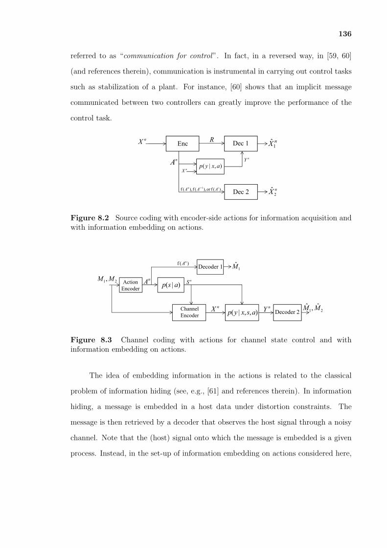
136
referred to as “communication for control”. In fact, in a reversed way, in [59, 60]
(and references therein), communication is instrumental in carrying out control tasks
such as stabilization of a plant. For instance, [60] shows that an implicit message
communicated between two controllers can greatly improve the performance of the
control task.
Dec 1Encn
X
nA
R
Dec 2
nX1ˆ
nY
nX 2ˆ
),|( axypn
X
)(for),(f),(f 1 iinAAA
−
Figure 8.2 Source coding with encoder-side actions for information acquisition andwith information embedding on actions.
Channel
Encoder
nX 21
ˆ,ˆ MMDecoder 2
Action
Encoder
nA n
S
nY
Decoder 1
21,MM
1M
),,|( asxyp
)|( asp
)(f nA
Figure 8.3 Channel coding with actions for channel state control and withinformation embedding on actions.
The idea of embedding information in the actions is related to the classical
problem of information hiding (see, e.g., [61] and references therein). In information
hiding, a message is embedded in a host data under distortion constraints. The
message is then retrieved by a decoder that observes the host signal through a noisy
channel. Note that the (host) signal onto which the message is embedded is a given
process. Instead, in the set-up of information embedding on actions considered here,

137
the (action) signal on which information is embedded is designed to optimize the
given communication task.
The set-up at hand is also related to the source coding model of [62], in which
an encoder communicates to two decoders and one of the decoders is able to observe
the source estimate produced by the other. For its duality with the classical channel
coding model studied in [63], the operation of the first decoder was referred to in
[62] as cribbing. Although the problem of interest here (in the source coding part) is
significantly different, in that the recipient of the embedded information is a decoder
“cribbing” the actions and not the estimates of another decoder, the solutions of the
two problems turn out to be related, as it will be discussed.
8.1.3 Contributions and Chapter Organization
The main contributions of this chapter are as follows.
• Decoder-side actions for side information acquisition: First, the model
in Figure 8.1 is considered, in which the problem of source coding with actions
taken at the decoder (Decoder 1) [4] is generalized by including an additional
decoder (Decoder 2). Decoder 2 is the recipient of a function of the action
sequence and is interested in reconstructing a lossy version of the source
measured at the encoder. A single-letter characterization of the set of all
achievable tuples of rate, distortions at the two decoders and action cost is
derived in Section 8.2 under the assumption that Decoder 2 observes a function
of the actions non-causally (Section 8.2.2), strictly causally (Section 8.2.3) or
causally (Section 8.2.4). An example is provided to shed light into the effect of
information embedding on actions in Section 8.2.5;
• Encoder-side actions for side information acquisition: Next, the set-up
in Figure 8.2 is considered, in which an additional decoder observing the actions
is added to the problem of source coding with actions taken at the encoder [4].

138
Section 8.3 derives the achievable rate-distortion-cost region in the special case
in which the channel pY |X,A(y|x, a) with source and action (X,A) as inputs and
side information Y as output is such that Y is a deterministic function of A;
• Actions for channel control and probing: Finally, the impact of infor-
mation embedding on actions for channel control is considered by studying the
set-up in Figure 8.3, which generalizes [44]. Specifically, a decoder (Decoder 1)
is added to the model in [44], that observes a function of the actions taken by
the encoder and wishes to decode part of the message that is intended for the
channel decoder (Decoder 2). A single-letter characterization of the achievable
capacity-cost region is obtained in Section 8.4. Finally, the special case of
actions for channel probing [45] is elaborated on with an example in Section
8.4.3.
8.2 Decoder-Side Actions for Side Information Acquisition
In this section, first, the system model is described for the set-up illustrated in Figure
8.1, Figure 8.4 and Figure 8.5 of source coding with decoder-side actions. Then, a
single letter characterization of the set of all achievable tuples of rate, distortions at
the two decoders and action cost is derived under the assumption that Decoder 2
observes the actions fully (non-causally) in Section 8.2.2, strictly causally in Section
8.2.3 and causally in Section 8.2.4. An example is provided in Section 8.2.5.
8.2.1 System Model
Here the problem corresponding to full observation of a function of the actions
is presented as per Figure 8.1. This model is referred to as having non-causal
action observation. The changes necessary to account for causal or strictly causal as
illustrated in Figure 8.4 and Figure 8.5 will be discussed in the appropriate sections
later. It is remarked that this definition does not entail any non-causal operation,

139
but only a larger estimation delay for Decoder 2 as compared to the causal cases in
Figure 8.4 and Figure 8.5. The model is defined by the probability mass functions
(pmfs) pX(x) and pY |AX(y|a, x), by the function f: A → B, and by discrete alphabets
X ,Y ,A,B, X1, X2, as follows. The source sequence Xn is such that Xi ∈ X for
i ∈ [1, n] is independent and identically distributed (i.i.d.) with pmf pX(x). The
Encoder measures sequence Xn and encodes it in a message M of nR bits, which is
delivered to Decoder 1. Decoder 1 receives messageM and selects an action sequence
An, where An ∈ An. The action sequence affects the quality of the measurement Y n
of sequence Xn obtained at the Decoder 1. Specifically, given An = an and Xn = xn,
the sequence Y n is distributed as p(yn|an, xn) =∏n
i=1 pY |A,X(yi|ai, xi). The cost of the
action sequence is defined by a cost function Λ: A →[0,Λmax] with 0 ≤ Λmax < ∞,
as Λ(an) =∑n
i=1 Λ(ai). The estimated sequence Xn1 ∈ X n
1 is then obtained as a
function of M and Y n. Decoder 2 observes a function of the action sequence An,
thus obtaining f(An) = (f(A1), ..., f(An)) ∈ Bn. Based on f(An), Decoder 2 obtains
an estimate Xn2 ∈ X n
2 within given distortion requirements. The estimated sequences
Xnj for j = 1, 2 must satisfy distortion constraints defined by functions dj(x, xj):
X × Xj → [0, Dj,max] with 0 ≤ Dj,max < ∞ for j = 1, 2, respectively. A formal
description of the operations at encoder and decoder follows.
Definition 8.1. An (n,R,D1, D2,Γ) code for the set-up of Figure 8.1 consists of a
source encoder
h(e): X n → [1, 2nR], (8.1)
which maps the sequence Xn into a message M ; an “action” function
h(a): [1, 2nR] → An, (8.2)
which maps the message M into an action sequence An; two decoders, namely
h(d)1 : [1, 2nR]× Yn → X n
1 , (8.3)

140
which maps the message M and the measured sequence Y n into the estimated
sequence Xn1 ;
h(d)2 : Bn → X n
2 , (8.4)
which maps the observed sequence f(An) into the the estimated sequence Xn2 ; such
that the action cost constraint Γ and distortion constraintsDj for j = 1, 2 are satisfied,
i.e.,
1
n
n∑i=1
E [Λ(Ai)] ≤ Γ (8.5)
and1
n
n∑i=1
E[dj(Xi, Xji)
]≤ Dj for j = 1, 2. (8.6)
Definition 8.2. Given a distortion-cost tuple (D1, D2,Γ), a rate R is said to be
achievable if, for any ϵ > 0, and sufficiently large n, there exists a (n,R,D1 + ϵ,D2 +
ϵ,Γ + ϵ) code.
Definition 8.3. The rate-distortion-cost function R(D1, D2,Γ) is defined asR(D1, D2,Γ) =
inf{R : the tuple (R,D1, D2,Γ)is achievable}.
8.2.2 Non-Causal Action Observation
In this section, a single-letter characterization of the rate-distortion region is derived
for the set-up in Figure 8.1 in which Decoder 1 observes the entire sequence fn(An)
prior to decoding.
Proposition 8.1. The rate-distortion-cost function R(D1, D2,Γ) for the source
coding problem with decoder-side actions and non-causal observation of the actions at
Decoder 2 illustrated in Figure 8.1 is given by
R(D1, D2,Γ) = minp(x2,a,u|x), g(U,Y )
I(X; X2, A) + I(X;U |X2, A, Y ), (8.7)

141
where the mutual information is evaluated with respect to the joint pmf
p(x, y, a, x2, u) = p(x)p(x2, a, u|x)p(y|x, a), (8.8)
for some pmf p(x2, a, u|x) such that the inequalities
E[dj(X, Xj)] ≤ Dj, for j = 1, 2, (8.9a)
E[Λ(A)] ≤ Γ, (8.9b)
and I(X; X2, f(A)) ≤ H(f(A)) (8.9c)
are satisfied for X1 = g(U, Y ) for some function g: U × Y → X1. Finally, U is
an auxiliary random variable whose alphabet cardinality can be constrained as |U| ≤
|X ||X2||A|+ 1 without loss of optimality.
At an intuitive level, in (8.7), the term I(X; X2, A) accounts for the rate needed
to instruct Decoder 1 about the actions A to be taken for the acquisition of the
side information Y , which are selected on the basis of the source X, and, at the
same time, to communicate the reconstruction X2 to Decoder 2. The additional rate
I(X;U |X2, A, Y ) is instead required to refine the description of the source X provided
via (X2, A) using an auxiliary codebook U for Decoder 1. Note that this rate is
conditioned on the side information Y , thanks to the rate saving obtained through
Wyner-Ziv binning. The condition (8.9c) ensures that, based on the observation of
f(A), Decoder 2 is able to reconstruct X2. The details of achievability follow as a
combination of the techniques proposed in [4] and [64, 62]. Below, the main ideas
are briefly outlined, since the technical details follow from standard arguments. The
proof of the converse is provided in Appendix T.
Sketch of the achievability proof : Fix a pmf (8.8) and define a random variable
B = f(A). The joint pmf p(x, y, a, x2, u, b) of variables (X, Y,A, X2, U,B) is obtained
by multiplying the right-hand side of (8.8) by the term1 1{b=f(a)}. In the scheme at
1The notation 1{S} is used for the indicator function of the event S.

142
hand, the Encoder first maps sequence Xn into a sequence Xn2 ∈ X n
2 using the joint
typicality criterion with respect to the joint pmf p(x, x2). This mapping requires a
codebook of rate I(X; X2) (see, e.g., [1, pp. 62-63]). Given the sequence Xn2 , the
sequence Xn is further mapped into a sequence Bn ∈ Bn using the joint typicality
criterion with respect to the joint pmf p(x, b|x2) where B = f(A), which requires a
codebook of rate I(X; f(A)|X2) for each sequence Xn2 . For later reference, every such
codebook is referred to as a bin in the following. Note that there exists one bin for
every sequence Xn2 . For each pair (Xn
2 , Bn), the sequence Xn is mapped into an action
sequence An using joint typicality with respect to the joint pmf p(x, a|x2, b), which
requires a codebook of rate I(X;A|X2, f(A)). Note that, by construction, Bn = f(An)
for each generated An. Finally, the source sequence Xn is mapped into a sequence Un
using the joint typicality criterion with respect to the joint pmf p(x, u|x2, a), which
requires a codebook of rate I(X;U |X2, A) for each pair (Xn2 , A
n).
The indices of codewords Xn2 , B
n and An are sent to Decoder 1, along with
the index for the codeword Un. For the latter, by leveraging the side information Y n
available at Decoder 1, the rate can be reduced to I(X;U |X2, A, Y ) by the Wyner-
Ziv theorem [1, p. 280]. Decoder 2 estimates the sequence Xn2 from the observed
sequence f(An) as follows: if there is only one bin containing the observed sequence
f(An), then Xn2 equals the sequence corresponding to such bin (recall that each bin
corresponds to one sequence Xn2 ). Otherwise, an error is decoded. To obtain a
vanishing probability of error, the sequence fn(An) should thus not lie within more
than one bin with high probability. The probability of the latter event can be upper
bounded by 2n(I(X;X2,f(A))−H(f(A)) since each sequence Bn is generated with probability
approximately 2−nH(f(A)) and there are 2nI(X;X2,f(A)) sequences Bn [62]. Therefore,
as long as I(X; X2, f(A)) ≤ H(f(A)), Decoder 1 is able to infer the conveyed bin
index with high probability. Finally, Decoder 1 produces the estimate Xn1 through a
symbol-by-symbol function as X1i = g(Ui, Yi) for i ∈ [1, n]. �

143
Remark 8.1. Assume that the action Ai is allowed to be a function, not only of
the message M as per (8.2), but also of the previous values of the side information
Y i−1, which is referred to as adaptive actions. Then, the rate-distortion-cost function
derived in Proposition 8.2 can generally be improved. This can be seen by considering
the case in which R = 0. In this case, if the actions were selected as per (8.2), then
the distortion at Decoder 2 would be forced to be maximal, i.e., D2 = D2,max, since
the actions A cannot depend in any way on the source X. Instead, by selecting A
as a function of the previously observed values of Y , Decoder 1 can provide Decoder
2 with information about X, thus decreasing the distortion D2. It is noted that the
usefulness of adaptive actions in this setting contrasts with the known fact that, in the
absence of Decoder 2, adaptive actions do not decrease the rate-distortion function
[26].
8.2.3 Strictly Causal Action Observation
The system model for the set-up in Figure 8.4, is similar to the one described in
Section 8.2.1 with the only difference the decoding function for Decoder 2 a time i is
given as
h(d)2i : Bi−1 → X2, (8.10)
which maps the strictly causally observed sequence f(Ai−1) = (f(A1), ..., f(Ai−1)) into
the ith estimated symbol X2i.
Proposition 8.2. The rate-distortion-cost function R(D1, D2,Γ) for the source
coding problem with decoder-side actions and strictly causal observation of the actions
at Decoder 1 as illustrated in Figure 8.4 is given by
R(D1, D2,Γ) = minp(x2,a,u|x), g(U,Y )
I(X; X2, A) + I(X;U |X2, A, Y ), (8.11)

144
Dec 1Encn
X
nA
R
nX 2ˆ
),|( xayp
nY
Dec 2
nX1ˆ
nX
)(f 1i-A.
Figure 8.4 Source coding with decoder-side actions for information acquisitionand with information embedding on actions. At time i, Decoder 2 has available thesamples f(Ai−1) = (f(A1), ..., f(Ai−1)) in a strictly causal fashion.
where the mutual information is evaluated with respect to the joint pmf
p(x, y, a, x2, u) = p(x)p(x2, a, u|x)p(y|x, a), (8.12)
for some pmf p(x2, a, u|x) such that the inequalities
E[dj(X, Xj)] ≤ Dj, for j = 1, 2, (8.13a)
E[Λ(A)] ≤ Γ, (8.13b)
and I(X; X2, f(A)) ≤ H(f(A)|X2) (8.13c)
are satisfied for X1 = g(U, Y ) for some function g: U × Y → X1. Finally, U is
an auxiliary random variable whose alphabet cardinality can be constrained as |U| ≤
|X ||X2||A|+ 1 without loss of optimality.
The only difference between the rate-distortion-cost function of Proposition 8.1
with non-causal action observation with respect to the case with strictly causal action
observation of Proposition 8.2 is the constraint (8.13c). Recall that the latter is needed
to ensure that Decoder 2 is able to recover the reconstruction X2. As detailed below,
the strict causality of the observation of the action at Decoder 2 calls for a block-
based encoding in which the actions carries information about the source sequence
as observed in two different blocks, namely the current block for Decoder 1 and the

145
future block for Decoder 2. This additional requirement causes the conditioning on
X2 in (8.13c), which generally increases the rate (8.11) with respect to the counterpart
(8.20) achievable with non-causal action observation. A sketch of the achievability
proof is provided below and is based on the techniques proposed in [64, 62] (see also
[65]). The proof of the converse is provided in Appendix U.
Sketch of the achievability proof : Fix a pmf (8.12) and define a random variable
B = f(A). The joint pmf p(x, y, a, x2, u, b) of variables (X,Y,A, X2, U,B) is obtained
by multiplying the right-hand side of (8.12) by the term 1{b=f(a)}. The “Forward
Encoding” and “Block Markov Decoding” strategy of [64, 62] (see also [65]) along
with the coding scheme of [4] is used. The scheme operates over multiple blocks
and Xn(l) is the portion of the source sequence encoded in block l. The sequence
f(An(l)) observed during block l is used in block l + 1 by Decoder 2 due to the strict
causality constraint. To this end, the action sequence f(An(l)) produced in block l
must carry information about the source sequence Xn(l + 1) corresponding to the
next block l + 1. Note that this is possible since encoder knows the entire sequence
Xn. At the same time, sequence An(l) should also perform well as an action sequence
to be used by Decoder 1 to estimate sequence Xn(l) for the current block. This is
accomplished as follows; In each block l, 2nI(X;X2) codewords Xn2 ∈ X n
2 are generated
according to the pmf p(x2). Next, 2nI(X;X2) bins are assigned to each codeword Xn2 ,
where each bin contains 2nI(X;f(A)|X2) codewords Bn ∈ Bn, generated according to pmf
p(b|x2). For each pair (Xn2 , B
n), a codebook of 2nI(X;A|X2,f(A)) codewords An ∈ An is
generated according to the joint pmf p(x, a|x2, b). Finally, a codebook of 2nI(X;U |X2,A)
codewords Un ∈ Un is generated according to the joint pmf p(x, u|x2, a). The latter
codebook is further binned into a codebook of rate I(X;U |X2, A, Y ) to leverage the
side information Y n available at Decoder 1 via the Wyner-Ziv theorem [1, p. 280].
For encoding, in each block l, a sequence Xn2 is selected from the X2−codebook
of block l to be jointly typical with the source sequence Xn(l) in the current block.

146
Instead, the bin index describes a Xn2 sequence in the X2−codebook of block (l+1)th
that is jointly typical with the source sequence Xn(l + 1) of the (l + 1)th block.
Moreover, given Xn2 and the bin index, a sequence An is chosen such that (An, Xn(l))
are jointly typical. Similarly, a sequence Un is selected for block l to be jointly typical
with the sequence of Xn(l) of block l.
Thanks to the observation of the actions, at block l + 1 Decoder 2 knows the
functions f(An(l)), and aims to find the bin index in which the corresponding codeword
Bn lies. As shown in [62], this is possible with vanishing probability of error, if
I(X; X2, f(A)) ≤ H(f(A)|X2). Note that the conditioning in the right-hand side is
due to the fact that the sequences Bn are generated conditioned on the sequence Xn2
representing a compressed version of the source for the current block l. The latter
does not bring any information regarding the desired sequence Xn(l + 1). �
Remark 8.2. From the proof of the converse in Appendix U, it follows, similarly to
[26], that, adaptive actions (see Remark 8.1) do not increase the rate-distortion-cost
function derived in Proposition 8.2.
8.2.4 Causal Action Observation
Dec 1Encn
X
nA
R
nX 2ˆ
),|( xayp
nY
Dec 2
nX1ˆ
nX
)(f iA.
Figure 8.5 Source coding with decoder-side actions for information acquisitionand with information embedding on actions. At time i, Decoder 2 has available thesamples f(Ai) = (f(A1), ..., f(Ai)) in a causal fashion.

147
The system model for the set-up in Figure 8.5, is similar to the one described
in Section 8.2.1 with the only difference the decoding function for Decoder 2 is
h(d)2i : Bi → X2, (8.14)
which maps the causally observed sequence f(Ai) = (f(A1), ..., f(Ai)) into the ith
estimated symbol X2i.
Proposition 8.3. The rate-distortion-cost function R(D1, D2,Γ) for the source
coding problem with decoder-side actions and causal observation of the actions
illustrated in Figure 8.5 is given by
R(D1, D2,Γ) = minp(v,a,u|x), g1(U,Y ), g2(V,f(A))
I(X;V,A) + I(X;U |V,A, Y ), (8.15)
where the mutual information is evaluated with respect to the joint pmf
p(x, y, a, u, v) = p(x)p(v, a, u|x)p(y|x, a), (8.16)
for some pmf p(v, a, u|x) such that the inequalities
E[dj(X, Xj)] ≤ Dj, for j = 1, 2, (8.17a)
E[Λ(A)] ≤ Γ, (8.17b)
and I(X;V, f(A)) ≤ H(f(A)|V ) (8.17c)
are satisfied for X1 = g1(U, Y ) and X2 = g2(V, f(A)) with some functions g1: U ×
Y → X1 and g2: V × B → X2, respectively. Finally, U and V are auxiliary random
variables whose alphabet cardinalities can be constrained as |U| ≤ |X ||V||A| + 1 and
|V| ≤ |X |+ 3, respectively, without loss of optimality.
The difference between the rate-distortion-cost function above with causal
and strictly causal action observation is given by the fact that, with causal action

148
observation, Decoder 2 can use the current value of the function f(A) for the estimate
of X2. This is captured by the fact that the Encoder provides Decoder 2 with an
auxiliary source description V , which is then combined with f(A) via a function
X2 = g2(V, f(A)) to obtain X2. The rate (8.15) and the constraint (8.17c) are changed
accordingly. The proof of the converse is given in Appendix U.
Remark 8.3. As seen in Appendix U, with adaptive actions, the rate-distortion-cost
function derived in Proposition 8.3 remains unchanged.
8.2.5 Binary Example
In this section, an example is provided to illustrate the effect of the communication
requirements of the additional decoder (Decoder 2) that observes a function of the
actions on the system performance. Binary alphabets as X = A = Y = {0, 1}
and a source distribution X ∼ Bern(12) are assumed. The distortion metrics are
assumed to be Hamming, i.e., dj(x, xj) = 0 if x = xj and dj(x, xj) = 1 otherwise
for j = 1, 2. Moreover, as shown in Figure 8.6, the side information Y at Decoder
1 is observed through a Z-channel for A = 0 or an S-channel for A = 1. No cost
constraint on the actions is assumed taken by Decoder 1 (which can be enforced by
choosing Λ(A) = A and Γ = 1), and f(A) = A. The example extends that of [4,
Section II-D] to a set-up with the additional Decoder 2. Under the requirement of
lossless reconstruction at Decoder 1, i.e., D1 = 0, the rate-distortion-cost function
R(0, D2,Γ = 1) with non-causal action observation is obtained from Proposition 8.1
by setting U = X1 = X, obtaining
R(0, D2, 1) = minp(x2,a|x)
I(X; X2, A) +H(X|X2, A, Y ), (8.18)
where the minimization is done under the constraints E[d2(X, X2)] ≤ D2 and
I(X; X2, A) ≤ H(A).
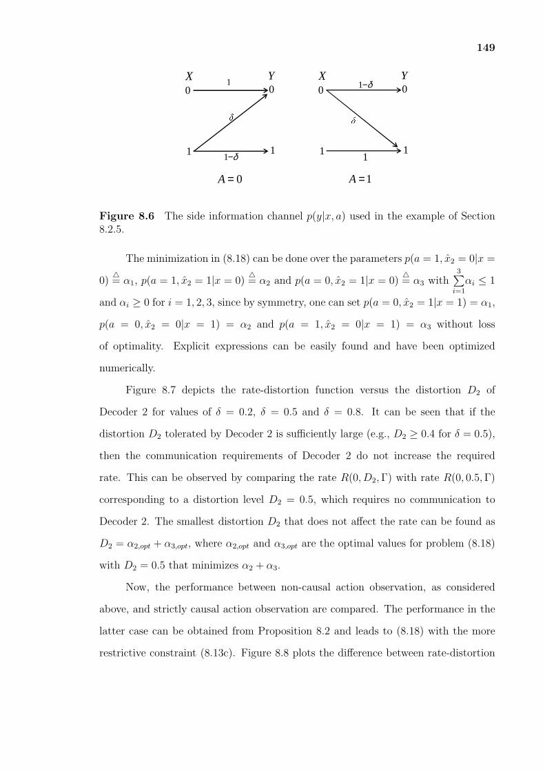
149
0
1
0
1
δ1 YX0
1
0
1
δ δ−1YX
1
0=A 1=A
δ−1
Figure 8.6 The side information channel p(y|x, a) used in the example of Section8.2.5.
The minimization in (8.18) can be done over the parameters p(a = 1, x2 = 0|x =
0)△= α1, p(a = 1, x2 = 1|x = 0)
△= α2 and p(a = 0, x2 = 1|x = 0)
△= α3 with
3∑i=1
αi ≤ 1
and αi ≥ 0 for i = 1, 2, 3, since by symmetry, one can set p(a = 0, x2 = 1|x = 1) = α1,
p(a = 0, x2 = 0|x = 1) = α2 and p(a = 1, x2 = 0|x = 1) = α3 without loss
of optimality. Explicit expressions can be easily found and have been optimized
numerically.
Figure 8.7 depicts the rate-distortion function versus the distortion D2 of
Decoder 2 for values of δ = 0.2, δ = 0.5 and δ = 0.8. It can be seen that if the
distortion D2 tolerated by Decoder 2 is sufficiently large (e.g., D2 ≥ 0.4 for δ = 0.5),
then the communication requirements of Decoder 2 do not increase the required
rate. This can be observed by comparing the rate R(0, D2,Γ) with rate R(0, 0.5,Γ)
corresponding to a distortion level D2 = 0.5, which requires no communication to
Decoder 2. The smallest distortion D2 that does not affect the rate can be found as
D2 = α2,opt + α3,opt, where α2,opt and α3,opt are the optimal values for problem (8.18)
with D2 = 0.5 that minimizes α2 + α3.
Now, the performance between non-causal action observation, as considered
above, and strictly causal action observation are compared. The performance in the
latter case can be obtained from Proposition 8.2 and leads to (8.18) with the more
restrictive constraint (8.13c). Figure 8.8 plots the difference between rate-distortion

150
0 0.05 0.1 0.15 0.2 0.25 0.3 0.35 0.4 0.45 0.5
0.4
0.5
0.6
0.7
0.8
0.9
1
Distortion D2
R
δ=0.2
δ=0.5δ=0.8
Figure 8.7 Rate-distortion function R(0, D2, 1) in (8.18) versus distortion D2 withthe side information channel in Figure 8.6 (non-causal side information).
0 0.1 0.2 0.3 0.4 0.5 0.6 0.7 0.8 0.9 10
0.005
0.01
0.015
δ
RS
C-R
NC
D2=0.1
D2=0.2
D2=0.3
Figure 8.8 Difference between the rate-distortion function (8.18) with non-causal(NC) and strictly causal (SC) action observation versus δ for values of distortionD2 = 0.1, 0.2 and 0.3.
function (8.18) for the case of non-causal and strictly causal action observation versus
δ for three values of distortion, namely D2 = 0.1, 0.2, 0.3. As shown, irrespective of the

151
value of distortion D2, for values of δ = 0 and δ = 1, the performance with non-causal
action observation is equal to that with strictly causal observation. This is due to the
facts that: i) for δ = 0, the side information Y is a noiseless measure of the source
sequence X for both A = 0 and A = 1 and thus there is no gain in making the actions
at Decoder 1 to be dependent of X, and thus X2; ii) for δ = 1, the side information
Y is independent of the source sequence X given both A = 0 and A = 1, and thus
it is without loss of optimality to choose actions at Decoder 1 to be independent of
X and X2. It is can be concluded that for both δ = 0 and δ = 1, causal action
observation, and in fact even selecting A to be independent of X, does not entail
any performance loss. Instead, for values 0 < δ < 1, it is generally advantageous for
Decoder 1 to select actions correlated with the source X, and hence some performance
loss is observed with strictly causal action observation owing to the more restrictive
constraint (8.13c). This reflects the need to cater to both Decoder 1 and Decoder 2
when selecting actions A, which requires description of two different source blocks.
Following similar arguments, it is also noted that, as the communication requirements
for Decoder 2 become more pronounced, i.e., as D2 decreases, the difference between
the rate-distortion function with non-causal and strictly-causal action observation
increases. The performance with causal action observation is intermediate between
full and strictly causal observation, and it is not shown here.
8.3 Encoder-Side Actions for Side Information Acquisition
In the previous section, the actions controlling the quality and availability of the
side information were taken by the decoder. In this section, following [4, Section
III], instead scenarios are considered in which the encoder takes the actions affecting
the side information of Decoder 1, as shown in Figure 8.2. Specifically, the encoder
takes actions An ∈ An, thus influencing the side information available to the Decoder
1 through a discrete memoryless channel p(y|x, a). Decoder 2 observes the action

152
sequence to obtain the deterministic function f(An) = (f(A1), ..., f(An)), or the
corresponding causal and strictly causal function, which is used to estimate the source
sequence subject to a distortion constraint.
An (n,R,D1, D2,Γ) code is defined similar to the previous sections with the
difference that the action encoder (8.2) maps directly the source sequence Xn into
the action sequence An, i.e.,
h(a): X n → An. (8.19)
As discussed in [4], even in the absence of Decoder 2, the problem at hand is
challenging. Therefore, focus is on certain special cases, first the special case in
which the side information channel p(y|x, a) is such that Y is a deterministic function
of A, i.e., Y = fY (A), and f(A) = A. This is solved in Proposition 8.4, and
generalized by the following remark to the case of all deterministic function f for
which H(fY (A)|f(A)) = 0. Following Proposition 8.4 is Proposition 8.5, where the
case H(f(Y )|fY (A)) = 0 is solved.
Proposition 8.4. The rate-distortion-cost function R(D1, D2,Γ) for the source
coding problem with encoder-side actions, non-causal, causal or strictly causal
observation of the actions illustrated in Figure 8.2 with f(A) = A and Y = fY (A)
is given by
R(D1, D2,Γ) = minp(u|x), p(x1|u,x), p(x2|u,x), p(a)
{I(X; X1, U)−H(fY (A))}+, (8.20)
where the information measures are evaluated with respect to the joint pmf
p(x, u, x1, x2, a) = p(x)p(u|x)p(x1|u, x)p(x2|u, x)p(a), (8.21)

153
for some pmfs p(u|x), p(x1|u, x), p(x2|u, x) and p(a) such that the inequalities
E[dj(X, Xj)] ≤ Dj, for j = 1, 2, (8.22a)
E[Λ(A)] ≤ Γ, (8.22b)
I(X;U) ≤ H(fY (A)) (8.22c)
and I(X; X2|U) ≤ H(A|fY (A)) (8.22d)
are satisfied. Finally, U is an auxiliary random variable whose alphabet cardinality
can be constrained as |U| ≤ |X ||X1||X2|+ 3 without loss of optimality.
Remark 8.4. The results above generalizes a number of known single-letter charac-
terizations. Notably, if D2 = D2,max, so that the distortion requirements of Decoder
2 are immaterial to the system performance, the result reduces to [4, Theorem 7].
Moreover, in the special case in which A = (A0, A2), Y = A0, R = R1, |A0| = 2R0 ,
|A2| = 2R2 , the model coincides with the lossy Gray-Wyner problem [66]2.
As detailed in the proof below, Proposition 8.4 establishes the optimality
of separate source-channel coding for the set-up in Figure 8.2 under the stated
conditions. In particular, the encoder compresses using a standard successive
refinement source code in which U represents the coarse description and X1, X2
two independent refinements. The indices of the coarse description U and of the
refined description X2 are sent on the degraded (deterministic) broadcast channel with
input A and outputs (A, t(A)) using superposition coding. Reliable compression and
communication is guaranteed by the two bounds (8.22c)-(8.22d). A further refined
description X1 is produced for Decoder 1, and the corresponding index is sent partly
over the mentioned broadcast channel and partly over the link of rate R, leading to
the rate (8.20). Details of the achievability proof can be found below, while the proof
of the converse is given in Appendix V.
2Note that here 2R0 and 2R2 are constrained to be integers.
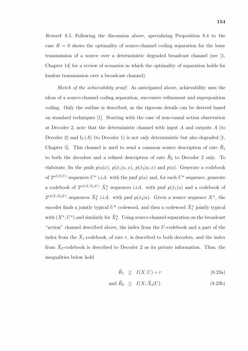
154
Remark 8.5. Following the discussion above, specializing Proposition 8.4 to the
case R = 0 shows the optimality of source-channel coding separation for the lossy
transmission of a source over a deterministic degraded broadcast channel (see [1,
Chapter 14] for a review of scenarios in which the optimality of separation holds for
lossless transmission over a broadcast channel).
Sketch of the achievability proof : As anticipated above, achievability uses the
ideas of a source-channel coding separation, successive refinement and superposition
coding. Only the outline is described, as the rigorous details can be derived based
on standard techniques [1]. Starting with the case of non-causal action observation
at Decoder 2, note that the deterministic channel with input A and outputs A (to
Decoder 2) and fY (A) (to Decoder 1) is not only deterministic but also degraded [1,
Chapter 5]. This channel is used to send a common source description of rate R1
to both the decoders and a refined description of rate R2 to Decoder 2 only. To
elaborate, fix the pmfs p(u|x), p(x1|u, x), p(x2|u, x) and p(a). Generate a codebook
of 2nI(X;U) sequences Un i.i.d. with the pmf p(u) and, for each Un sequence, generate
a codebook of 2nI(X;X1|U) Xn1 sequences i.i.d. with pmf p(x1|u) and a codebook of
2nI(X;X2|U) sequences Xn2 i.i.d. with pmf p(x2|u). Given a source sequence Xn, the
encoder finds a jointly typical Un codeword, and then a codeword Xn1 jointly typical
with (Xn, Un) and similarly for Xn2 . Using source-channel separation on the broadcast
“action” channel described above, the index from the U -codebook and a part of the
index from the X1-codebook, of rate r, is described to both decoders, and the index
from X2-codebook is described to Decoder 2 as its private information. Thus, the
inequalities below hold
R1 ≥ I(X;U) + r (8.23a)
and R2 ≥ I(X; X2|U). (8.23b)

155
The capacity region of the broadcast channel is given by the conditions [1, Chapter
9], R1 ≤ H(fY (A)) and R1 + R2 ≤ H(A), and thus the following rates are achievable
R1 ≤ H(fY (A)) (8.24a)
and R2 ≤ H(A|fY (A)). (8.24b)
Finally the remaining part of the index of codeword Xn1 is sent through the direct
rate R, leading to the condition
R ≥ I(X; X1|U)− r. (8.25)
Combining (8.23), (8.24) and (8.25), and using Fourier-Motzkin elimination, one can
obtain
R ≥ I(X; X1, U)−H(fY (A)) (8.26)
and (8.29c)-(8.22d). The distortion and cost constraints are handled in a standard
manner and hence the details are omitted.
It remains to discuss how to handle the case of causal or strictly causal action
observation. Given the converse result in Appendix V, it is enough to show that
(8.20)-(8.22) is achievable also with strictly causal and causal action observation. This
can be simply accomplished by encoding in blocks as per achievability of Proposition
8.2 and Proposition 8.3. Specifically, in each block the encoder compresses the source
sequence corresponding to the next block. Decoder 2 then operates as above, while
Decoder 1 can recover all source blocks at the end of all blocks. �
Remark 8.6. The scenario solved above is when the action observation is perfect, i.e.,
f(A) = A. The result also carries verbatim for the more general case where f(A) is
a generic function as long as H(fY (A)|f(A)) = 0. The expressions of the rate region
remain the same as in the proposition above except that A is replaced by f(A).

156
Proposition 8.4 characterizes the optimal performance for the case when
Decoder 2 has a better information about the actions taken by the encoder than
Decoder 1 in the sense that H(fY (A)—f(A)) = 0. It is noted here that a similar
characterization can be given also for the dual setting in which H(f(A)—fY (A)) = 0
so that Decoder 1 has the better observation about the actions.
Proposition 8.5. The rate-distortion-cost function R(D1, D2,Γ) for the source
coding problem with encoder-side actions, non-causal, causal or strictly causal
observation of the actions illustrated in Figure 8.2 with H(f(A)|fY (A)) = 0, is given
by
R(D1, D2,Γ) = minp(a), p(x1,x2|x)
{I(X; X1, X2)−H(fY (A))}+, (8.27)
where the information measures are evaluated with respect to the joint pmf
p(x, x1, x2, a) = p(x)p(x1, x2|x)p(a), (8.28)
such that the following inequalities are satisfied,
E[dj(X, Xj)] ≤ Dj, for j = 1, 2, (8.29a)
E[Λ(A)] ≤ Γ, (8.29b)
I(X; X2) ≤ H(f(A)). (8.29c)
The converse follows similarly as that for Proposition 8.4 where instead of U
in the converse, X2 is used, as knowing Y n = fY (An) implies knowing f(An), due
to the assumption H(f(A)|fY (A)) = 0. The achievability is outlined for only for
the non-causal case (the achievability for strictly causal and causal case uses block
coding ideas as in Proposition 8.4). A successive refinement codebook is generated by
drawing 2nI(X;X2) codewords Xn2 , and, for each codeword Xn
2 , a number 2nI(X;X1|X2) of

157
codewords Xn1 . As for Proposition 8.4, the indices of these two codebooks obtained via
standard joint typicality encoding are sent through the degraded broadcast channel
p(y, b|a) = 1{y=fY (A),b=f(A)}. Splitting the rate for the index of codeword Xn1 so that
a rate R is sent over the direct link to Decoder 1, reliability of compression and
communication over the “action” broadcast channel is guaranteed if
I(X; X2) ≤ H(f(A)) (8.30)
I(X; X2) + I(X; X1|X2)−R ≤ H(f(A), fY (A)) = H(fY (A)), (8.31)
where the latter inequality implies R ≥ I(X; X1, X2) − H(fY (A)). The proof is
concluded using the usual steps. �
8.4 Actions for Channel State Control and Probing
In this section, the impact of information embedding on actions for the set-up of
channel coding with actions of [44] is considered. To this end, consider the model in
Figure 8.3, in which Decoder 1, based on the observation of a deterministic function
of the actions, wishes to retrieve part of the information destined to Decoder 2. Note
that for simplicity of notation here the additional encoder that observes the actions
is denoted as Decoder 1, rather than Decoder 2 as done above. Also, it is emphasized
that in the original set-up of [44], Decoder 1 was not present.
8.4.1 System Model
The system is defined by the pmfs p(x), p(y|x, s, a), p(s|a), function f: A → B and
by discrete alphabets X ,A, B, S, and Y . Given the messages (M1,M2), selected
randomly from the set M1 × M2 = [1, 2nR1 ] × [1, 2nR2 ], an action sequence An ∈
An is selected by the Encoder. Decoder 1 observes the signal Bn = f(An) as a
deterministic function of the actions, and estimates message M1. Note that the
notation here implies a “non-causal” observation of the actions, but it is easy to

158
see that the results below hold also with causal and strictly causal observation of
the actions. Moreover, the state sequence Sn ∈ Sn is generated as the output of
a memoryless channel p(s|a) and p(bn, sn|an) =∏n
i=1 p(si|ai)1{bi=f(ai)} holds for an
action sequence An = an. The input sequence Xn ∈ X n is selected on the basis of
both messages (M1,M2) and of the state sequence Sn by the Encoder. The action
sequence An and the input Xn have to satisfy an average cost constraint defined by
a function γ : A × X → [0,∞), so that the cost for the input sequences an and xn
is given by γ(an, xn) = 1n
∑ni=1 γ(ai, xi). Given Xn = xn, Sn = sn and An = an,
the received signal is distributed as p(yn|xn, sn, an) =∏n
i=1 p(yi|xi, si, ai). Decoder 2,
having received the signal Y n, estimates both messages (M1,M2).
The setting includes the semi-deterministic broadcast channel with degraded
message sets [67] (see also [1, Ch. 8]) as a special case by setting X to be constant
and Y = S, and the channel with action-dependent states studied in [44] for R1 = 0.
Definition 8.4. An (n,R0, R1,Γ, ϵ) code for the model in Figure 8.3 consists of an
action encoder
h(a): M1 ×M2 → An, (8.32)
which maps message (M1,M2) into an action sequence An; a channel encoder
h(e): M1 ×M2 × Sn → X n, (8.33)
which maps message (M1,M2) and the state sequence Sn into the sequence Xn; two
decoding functions
h(d)1 : Bn → M1, (8.34)
and h(d)2 : Yn → M1 ×M2, (8.35)
which map the sequences Bn and Y n into the estimated messages M1 and (M1, M2),
respectively; such that the probability of error in decoding the messages (M1,M2) is

159
small,
Pr[h(d)1 (Bn) =M1] ≤ ϵ, (8.36)
and Pr[h(d)2 (Y n) = (M1,M2)] ≤ ϵ, (8.37)
and the cost constraint is satisfied, i.e.,
1
n
n∑i=1
E [γ(Ai, Xi)] ≤ Γ + ϵ. (8.38)
Given a cost Γ, a rate pair (R1, R2) is said to be achievable for a cost-constraint
Γ if, for any ϵ > 0 and sufficiently large n, there a exists a (n,R1, R2,Γ, ϵ) code.
The goal is to characterize the capacity-cost region C(Γ), which is the closure of all
achievable rate pairs (R1, R2) for the given cost Γ.
8.4.2 Capacity-Cost Region
In this section, a single-letter characterization of the capacity-cost region is derived.
Proposition 8.6. The capacity-cost region C(Γ) for the system in Figure 8.3 is given
by the union of all rate pairs (R1, R2) such that the inequalities
R1 ≤ H(f(A)) (8.39a)
and R1 +R2 ≤ I(A,U ;Y )− I(U ;S|A), (8.39b)
are satisfied, where the mutual informations are evaluated with respect to the joint
pmf
p(a, s, u, x, y) = p(a)p(s|a)p(u|s, a)1{x=g(u,s)}p(y|x, s, a), (8.40)
for some pmfs p(a), p(u|s, a) and function g: U × S → X such that
E[γ(A,X)] ≤ Γ. (8.41)

160
Finally, one can set |U| ≤ |X ||S||A|+ 1 without loss of optimality.
The proof of converse is an immediate consequence of cut-set arguments and
of the proof of the upper bound obtained in [44, Theorem 1]. Specifically, inequality
(8.39a) follows by considering the cut around Decoder 1, while the inequality (8.39b)
coincides with the bound derived in [44, Theorem 1] on the rate that can be
communicated between the Encoder and Decoder 2 with no regards for Decoder 13.
The achievability requires rate splitting, superposition coding and the coding strategy
proposed in [44, Theorem 1]. A sketch of proof of the achievability is relegated to
Appendix W.
Channel Encoder
nX 21ˆ,ˆ MM
Decoder 2
Probing Logic
nA nS
nY
Decoder 1
21,MM
1M
0
1
1
5.05.0
5.0
5.0
0=S
1=S
0 . .
1 . . 1
S w p
S w p
εε
== −
1
nS
nS
Switch
0
1
0
1
0
1
neS
Figure 8.9 Channel coding with actions for channel state probing and withinformation embedding on actions.
8.4.3 Probing Capacity
Here, an example is provided to illustrate the effect of the communication requirements
of the action-cribbing decoder on the system performance. Consider the communi-
cation system shown in Figure 8.9, where the states is known to Decoder 2. It is
further assumed that actions are binary, such that, if A = 1, the channel encoder
observes the state S, and if A = 0, it does not obtain any information about S.
3The cardinality constraints follow from [44, Theorem 1]

161
This problem is modeled by defining the state information available at the encoder
as Se = u(S,A), where u(S, 1) = S and u(S, 0) = e, where represents as “erasure”
symbol. Following [45], this problem is referred to as having a “probing” encoder.
The channel encoder maps the state information Sne and messages M1,M2
into a codeword Xn (see Figure 8.9). Moreover, two cost constraints, namely
1n
∑ni=1 E [γa(Ai)] ≤ ΓA and 1
n
∑ni=1 E [γx(Xi)] ≤ ΓX are imposed for given action
input cost functions γa : A → [0,Λa,max] and γx : X → [0,Λx,max] with 0 ≤
Λa,max <∞ and 0 ≤ Λx,max <∞, respectively. In [45, Theorem 1], a correspondence
was proved between the set-up of a probing encoder and that of action dependent
states. Using [45, Theorem 1] and Proposition 8.6, one can easily obtain that the
capacity-cost region C(ΓA,ΓX) for the system in Figure 8.9 is given by the union of
all rate pairs (R1, R2) such that the inequalities
R1 ≤ H(A|Q) (8.42a)
and R1 +R2 ≤ I(X;Y |S,Q), (8.42b)
are satisfied, where the mutual informations are evaluated with respect to the joint
pmf
p(q, a, s, se, x, y) = p(q)p(a|q)p(s)1{se=u(s,a)}p(x|se, a, q)p(y|x, s), (8.43)
for some pmfs p(q), p(a|q), p(x|se, a, q) such that E[γa(A)] ≤ ΓA and E[γx(X)] ≤ ΓX .
Now, (8.42a)-(8.42b) are applied to the channel shown in Figure 8.9 in which
alphabets are binary X = Y = S = {0, 1}, S is a Bern(1 − ϵ) variable for 0 ≤ ϵ ≤ 1
and the channel is a binary symmetric with flipping probability 0.5 if S = 0 (“bad”
channel state) and 0 if S = 1 (“good” channel state).
To evaluate the maximum achievable sum-rate R1+R2 for a given rate R1, let’s
define Pr[A = 1] = γ, Pr[X = 1|Se = 1, A = 1] = p1 and Pr[X = 1|Se = e, A = 0] =
p2, and set Pr[X = 1|Se = 0, A = 1] = 0 without loss of optimality. The maximum

162
sum-rate R1 + R2 for a given rate R1 is then obtained from (8.42b) by solving the
problem
R1 +R2 = max0≤p1,p2,γ≤1
γ(1− ϵ)H(p1) + (1− γ)(1− ϵ)H(p2), (8.44)
under the constraint E[X] = p1γ(1 − ϵ) + p2(1 − γ) ≤ ΓX , E[A] = γ ≤ ΓA and
H(A) = H(γ) ≥ R1. Note that the last constraint imposes that the rate achievable
by the Decoder 1 is larger than R1 as per (8.42a).
The sum-rate in (8.44) is shown in Figure 8.10 for ϵ = 0.5, ΓA = 1 and different
values of R1. It can be seen that, for sufficiently small values of the cost constraint
ΓX , increasing the communication requirements, i.e., R1, of the Decoder 1, reduces
the achievable sum-rate R1 + R2. This is due to the fact that increasing R1 requires
to encode more information in the action sequence, which in turn reduces the portion
of the actions that can be set to A = 1, i.e., Pr[A = 1]. As a result, the encoder is
less informed about the state sequence and thus bound to waste some power on bad
channel states.
Remark 8.7. The communication requirements of Decoder 1 need not necessarily
affect the system performance. For instance, consider the example 1 in [45, Section
V.A], which includes a probing encoder as in Figure 8.9 but transmitting over a
different channel. There, it turns out that it is sufficient to have Pr[A = 1] & 0.2
in order to achieve the same performance that can be achieved with full encoder
channel state information. Therefore, the additional constraint on the rate of Decoder
1 (8.42a), namely R1 ≥ H(A), does not affect the sum-rate achievable in this example
for any rate R1 ∈ [0, 1].
8.5 Concluding Remarks
There is a profound interplay between actuation and communication in that both
actuation can be instrumental to improve the efficiency of communication, and, vice

163
0.1 0.15 0.2 0.25 0.3 0.35 0.40.32
0.34
0.36
0.38
0.4
0.42
0.44
0.46
0.48
0.5
ΓX
R1+R2
R1=0
R1=0.5
R1=0.9
Figure 8.10 Sum-rate R1 + R2 versus the input cost constraint ΓX for values ofR1 = 0, R1 = 0.5 and R1 = 0.9.
versa, communication, implicit or explicit, can provide an essential tool to improve
control tasks. This work has focused on the first type of interplay, and has investigated
the implications of embedding information directly in the actions for the aim of
communicating with a separate decoder. The communication requirements of this
decoder are generally in conflict with the goal of improving the efficiency of the
given communication link. This performance trade-off has been studied here for both
source and channel coding. The results provided in this chapter allow to give a
quantitative answer to the questions posed in Section 8.1.1 regarding the impact of
the requirements of action information embedding on the system performance. They
also shed light into the structure of optimal embedding strategies, which turns out to
be related, for the source coding model, with the strategies studied in [62, 64].
The investigation on the theme of information embedding on actions can be
further developed in a number of directions, including models with memory [56, 28]
and with multiple terminals [23, 55, 27]. It is also noted that results akin to the ones

164
reported here can be developed assuming causal state information at the decoder for
source coding problems or causal state information at the transmitter.

APPENDIX A
PROOF OF PROPOSITION 3.1
First, it is observed that from Definition 3.1, since distortion and CR constraints(3.8) and (3.9) depend only on the marginal pmfs p(x, y1) and p(x, y2), so does therate-distortion function. Therefore, in the proof, one can assume, without loss ofgenerality, that the joint pmf p(x, y1, y2) satisfies the Markov chain condition X −Y2 − Y1 so that it factorizes as (cf. (3.10))
p(x, y1, y2) = p(x, y2)p(y1|y2). (A.1)
Consider an (n,R,D1 + ϵ,D2 + ϵ, ϵ) code, whose existence is required forachievability by Definition 3.1. By the CR requirements (3.9), first it is observedthat the following Fano inequalities hold
H(ψj(Xn)|hj(g(Xn), Y n
j )) ≤ nδ(ϵ), for j = 1, 2, (A.2)
for n sufficiently large, where δ(ϵ) = nϵlog|X |+Hb(ϵ). Moreover, one can write
nR = H(J) ≥ H(J |Y n1 ) (A.3a)
(a)= H(J |Y n
1 Yn2 ) + I(J ;Y n
2 |Y n1 ), (A.3b)
where (a) follows by the definition of mutual information. From now on, to simplifynotation, explicit the dependence of ψj, gj and hj on Xn and (J, Y n
j ), respectively,is not made. Also, ψji is defined as the ith symbol of the sequence ψj so that ψj =(ψj1, ..., ψjn).
The first term in (A.3b), H(J |Y n1 Y
n2 ), can be treated as in [8, Section V.A.], or,
more simply, one can proceed as follows:
H(J |Y n1 Y
n2 )
(a)= I(J ;Xn|Y n
1 Yn2 ) (A.4a)
(b)
≥ I(h1h2;Xn|Y n
1 Yn2 ) (A.4b)
= I(h1h2ψ1ψ2;Xn|Y n
1 Yn2 )− I(ψ1ψ2;X
n|Y n1 Y
n2 h1h2) (A.4c)
(c)
≥ I(ψ1ψ2;Xn|Y n
1 Yn2 )− I(ψ1ψ2;X
n|Y n1 Y
n2 h1h2) (A.4d)
(d)= I(ψ1ψ2;X
n|Y n2 )−H(ψ1ψ2|Y n
1 Yn2 h1h2)
+H(ψ1ψ2|Y n1 Y
n2 h1h2X
n) (A.4e)(e)
≥ I(ψ1ψ2;Xn|Y n
2 )− nδ(ϵ) (A.4f)
(f)
≥n∑
i=1
I(ψ1iψ2i;Xi|Y2i)− nδ(ϵ), (A.4g)
165
166
where (a) follows because J is a function of Xn; (b) follows since h1 and h2 arefunctions of (J, Y n
1 ) and (J, Y n2 ), respectively ; (c) follows by using the Markov chain
(ψ1, ψ1, Xn)—Y n
2 —Y n1 ; (d) follows by the chain rule of mutual information and since
mutual information is non-negative; (e) follows by (R.2a) and since entropy is non-negative; and (f) follows by the chain rule for entropy, since Xn and Y n
2 are i.i.d.,and due to the fact conditioning decreases entropy.
Similarly, the second term in (A.3b), namely, I(J ;Y n2 |Y n
1 ), leads to
I(J ;Y n2 |Y n
1 )(a)
≥ I(h1;Yn2 |Y n
1 ) (A.5a)
= I(h1ψ1;Yn2 |Y n
1 )− I(ψ1;Yn2 |Y n
1 h1) (A.5b)(b)
≥ I(ψ1;Yn2 |Y n
1 )−H(ψ1|Y n1 h1) +H(ψ1|Y n
1 Yn2 h1) (A.5c)
(c)
≥ I(ψ1;Yn2 |Y n
1 )− nδ(ϵ) (A.5d)
(d)
≥n∑
i=1
I(ψ1i;Y2i|Y1i)− nδ(ϵ), (A.5e)
where (a) follows because h1 is a function of J and Y n1 ; (b) follows by the chain rule
of mutual information and since mutual information is non-negative; (c) follows by(R.2a) and since entropy is non-negative; and (d) follows by the chain rule for entropy,since Y n
2 and Y n1 are i.i.d., and due to the fact conditioning decreases entropy. From
(A.3b), (A.4g), and (A.5e), it is also true that
nR ≥n∑
i=1
I(ψ1iψ2i;Xi|Y2i) + I(ψ1i;Y2i|Y1i)− nδ(ϵ) (A.6a)
(a)=
n∑i=1
I(Xi;ψ1i|Y1i) + I(Xi;ψ2i|Y2iψ1i)− nδ(ϵ), (A.6b)
where (a) follows because of the Markov chain relationship (ψ1i, ψ2i)−Xi−Y2i−Y1i,
for i = 1, ..., n. By defining Xji = ψji with j = 1, 2 and i = 1, ..., n, the proof isconcluded as in [8].

APPENDIX B
PROOF OF PROPOSITION 3.2
As explained in the text, it is only required to focus on the case where D2 ≤ D1 ≤ σ2x.
As per the discussion in Appendix A, one can assume, without loss of generality, thatthe Markov chain relationship X − Y2 − Y1 holds, so that
Y2 = X + Z2 (B.1a)
and Y1 = Y2 + Z1, (B.1b)
where Z1 ∼ N (0, N1) is independent of (X,Z2).First a converse is proved. Calculating the rate-distortion function in (3.14)
requires minimization over the pmf p(x1, x2|x) under the constraint (3.13). Aminimizing p(x1, x2|x) exists by the Weierstrass theorem due to the continuity of themutual information and the compactness of the set of pmfs defined by the constraint(3.13)[68]. Fixing one such optimizing p(x1, x2|x), the rate-distortion function (3.14)can be written as
RCRHB(D1, D2) = I(X; X2|Y2) + I(X1;Y2|Y1). (B.2)
The first term in (B.2), i.e., I(X; X2|Y2), can be easily bounded using the approachin [8, p. 5007]. Specifically, the following holds
I(X; X2|Y2) = h(X|Y2)− h(X|X2Y2)
= h(X|X + Z2)− h(X − X2|X2, X2 + (X − X2) + Z2)
= h(X|X + Z2)− h(X − X2|X2, (X − X2) + Z2)(a)
≥ h(X|X + Z2)− h(X − X2|(X − X2) + Z2)
(b)
≥ 1
2log2
(2πe
σ2x
1 + σ2x
N2
)− 1
2log2
(2πe
D2
1 + D2
N2
)
=1
2log2
(σ2x
σ2x +N2
· D2 +N2
D2
), (B.3)
where (a) follows because conditioning decreases entropy; and (b) follows from themaximum conditional entropy lemma [1, p. 21], which implies that h(E|E + Z2) ≤12log2(2πeσ
2E|E+Z2
) with E = X−X2. In fact, it is true that σ2E|E+Z2
≤ D2
1+D2N2
, since the
conditional variance σ2E|E+Z2
is upper bounded by the linear minimum mean square
error of the estimate of E given E + Z2. This mean square error is given by D2
1+D2N2
,
since E[E2] ≤ D2 and since Z2 is independent of E due to the factorization (3.12)
167
168
and to the independence of X and Z2. For the second term in (B.2), the followingholds:
I(X1;Y2|Y1) = h(Y2|Y1)− h(Y2|Y1, X1)
=1
2log2
(2πe
N1(N2 + σ2x)
N1 +N2 + σ2x
)− h(Y2|Y1, X1). (B.4)
Moreover, it can be evaluated as
h(Y2|Y1, X1) = h(Y2, Y1|X1)− h(Y1|X1)
= h(Y2|X1) + h(Y1|Y2, X1)− h(Y1|X1)
= h(Y2|X1)− h(Y2 + Z1|X1) + h(Y2 + Z1|Y2, X1)
(a)= h(Y2|X1)− h(Y2 + Z1|X1) +
1
2log2(2πeN1), (B.5)
where (a) follows because Z1 is independent of Y2 and of X1, due to the factorization(3.12) and due to the independence of Z1 and X. Next, a lower bound is obtained on
the term h(Y2+ Z1|X1) in (B.5) as a function of h(Y2|X1) by using the entropy powerinequality (EPI) [1, p. 22]. Specifically, by using the conditional version of EPI [1, p.22], it holds that
22h(Y2+Z1|X1) ≥ 22h(Y2|X1) + 22h(Z1|X1)
(a)= 22h(Y2|X1) + 22h(Z1)
= 22h(Y2|X1) + 2πeN1, (B.6)
where (a) follows because Z1 is independent of X1 as explained above. The first twoterms in (B.5) can thus be bounded as
h(Y2|X1)− h(Y2 + Z1|X1) ≤ h(Y2|X1)−1
2log(22h(Y2|X1) + 2πeN1)
=1
2log2
(22h(Y2|X1)
22h(Y2|X1) + 2πeN1
)(a)
≤ log2
(2πe(D1 +N2)
2πe(D1 +N2) + 2πeN1
), (B.7)
where (a) follows because log2
(22h(Y2|X1)
22h(Y2|X1)+2πeN1
)is an increasing function of h(Y2|X1)
and h(Y2|X1) ≤ 12log2(2πe(D1 +N2)), as can be proved by using the same approach
used for the bounds (a) and (b) in (B.3). By substituting (B.7) into (B.5), and usingthe result in (B.4), one can obtain
I(X1;Y2|Y1) ≥ 1
2log2
(2πe
N1(N2 + σ2x)
N1 +N2 + σ2x
)− 1
2log2
(2πe
N1(D1 +N2)
D1 +N2 +N1
)=
1
2log2
((N2 + σ2
x)(D1 +N2 +N1)
(N1 +N2 + σ2x)(D1 +N2)
). (B.8)

169
Finally, by substituting (B.3) and (B.8) into (B.2), the lower bound is obtained as
RCRHB(D1, D2) ≥ 1
2log2
(σ2x
σ2x +N2
· D2 +N2
D2
)+
1
2log2
((N2 + σ2
x)(D1 +N2 +N1)
(N1 +N2 + σ2x)(D1 +N2)
)=
1
2log2
(σ2x
(σ2x +N1 +N2)
· (D1 +N1 +N2)(D2 +N2)
(D1 +N2)D2
). (B.9)
For achievability, (3.14) is calculated with X = X2 + Q2 and X2 = X1 + Q1,where Q1 ∼ N (0, D1 −D2) and Q2 ∼ N (0, D2) are independent of each other and of
(X1,Z1, Z2). This leads to the upper bound
RCRHB(D1, D2) ≤ I(X; X1X2|Y2) + I(X1;Y2|Y1)
= I(X; X2|Y2) + I(X1;Y2|Y1)= h(X|Y2)− h(X|Y2, X2) + h(Y2|Y1)− h(Y2|Y1, X1)
= h(X|X + Z2)− h(X2 +Q2|X2 +Q2 + Z2, X2)
+h(X + Z2|X + Z2 + Z1)
−h(X1 +Q1 +Q2 + Z2|X1 +Q1 +Q2 + Z2 + Z1, X1)
= h(X|X + Z2)− h(Q2|Q2 + Z2) + h(X + Z2|X + Z2 + Z1)
−h(Q1 +Q2 + Z2|Q1 +Q2 + Z2 + Z1)
(a)=
1
2log2
(2πe
σ2x
1 + σ2x
N2
)− 1
2log2
(2πe
D2
1 + D2
N2
)
+1
2log2
(2πe
σ2x +N2
1 + σ2x+N2
N1
)− 1
2log2
(2πe
D1 +N2
1 + D1+N2
N1
)
=1
2log2
(σ2x
(σ2x +N1 +N2)
· (D1 +N1 +N2)(D2 +N2)
(D1 +N2)D2
), (B.10)
where (a) follows using h(A|A + B) = 12log2
(2πe SA
1+SASB
), for A and B being
independent Gaussian sources with A ∼ N (0, SA) and B ∼ N (0, SB). By comparing(B.9) with (B.10), the proof is completed.

APPENDIX C
PROOF OF (3.23)
Here, it is proved that (3.2) equals (3.23) for the given sources. For the converse, thefollowing holds
I(X; X|Y ) = H(X|Y )−H(X|X, Y )
= p− pH(X|X, Y = X)− (1− p2)H(X|X, Y = X)
= p− pH(X|X, Y = X)
= p− pH(X|X)
= p− pH(X ⊕ X|X)(a)
≥ p− pH(X ⊕ X)≥ p− pH(D)= p(1−H(D)), (C.1)
where (a) follows because conditioning decreases entropy. Achievability follows by
calculating (3.2) with X = X ⊕Q where Q ∼ Ber(D).
170

APPENDIX D
PROOF OF PROPOSITION 3.3
As explained in the text, it is only required to focus on the case whereD2 ≤ D1 ≤ 1/2.As for Appendix A and Appendix B, one can assume, without loss of generality, thatthe joint pmf of (x, y1, y2) factorizes as (A.1) as shown Figure 3.7. First, a converseis proved. Similar to (B.2), the rate-distortion function (3.14) can be written as
RCRHB(D1, D2) = I(X; X2|Y2) + I(X1;Y2|Y1), (D.1)
where the mutual information terms are calculated with a distribution p(x1, x2|x)minimizing (3.14) under the constraint (3.13). The first term in (D.1), i.e.,
I(X; X2|Y2), can be easily bounded by following the same steps used in the derivationof (C.1), leading to
I(X; X2|Y2) ≥ p2(1−H(D2)). (D.2)
For the second term in (D.1), instead the following holds
I(X1;Y2|Y1) = H(Y2|Y1)−H(Y2|Y1, X1)
= H(Y2|Y1)−H(Y2, Y1|X1) +H(Y1|X1) (D.3)
= H(Y2|Y1)−H(Y2|X1)−H(Y1|X1, Y2) +H(Y1|X1) (D.4)(a)= H(Y2|Y1)−H(Y2|X1)−H(Y1|Y2) +H(Y1|X1), (D.5)
where (a) follows because of the Markov chain condition Y1 − Y2 − X1. The secondterm in the right-hand side of (D.5) can be evaluated as
H(Y2|X1) = H(Y2, X|X1)−H(X|Y2, X1)
= H(X|X1) +H(Y2|X, X1)−H(X|Y2, X1)
= H(X|X1) +H(Y2|X)− p2H(X|Y2 = X, X1)
−(1− p2)H(X|Y2 = X, X1)(a)= H(X|X1) +H(p2)− p2H(X|X1)
= H(p2) + (1− p2)H(X|X1) (D.6)
where (a) follows because H(Y2|X) = H(p2). The fourth term in the right-hand sideof (D.5) can similarly be evaluated as
H(Y1|X1) = H(p1) + (1− p1)H(X|X1). (D.7)
171

172
Substituting (D.6) and (D.7) in (D.5), it holds that
I(X1;Y2|Y1) = H(p1) + (1− p1)H(X|X1)− (H(p2) + (1− p2)H(X|X1))+H(Y2|Y1)−H(Y1|Y2)
= H(p1)−H(p2)− (p1 − p2)H(X|X1) +H(Y2)−H(Y1)(a)
≥ (p1 − p2)− (p1 − p2)H(D1) (D.8)
where (a) follows since H(Y2) = H(p2) + (1− p2) and H(Y1) = H(p1) + (1− p1) and
due to the inequality H(X|X1) ≤ H(D1). Substituting (D.8) and (D.2) into (D.1), itis true that
RCRHB(D1, D2) ≥ p2(1−H(D2)) + (p1 − p2)(1−H(D1))
= p1(1−H(D1)) + p2(H(D1)−H(D2)). (D.9)
For achievability, (3.14) is calculated with X = X2 ⊕ Q2 and X2 = X1 ⊕ Q1,where Q1 ∼ Ber(D1 ∗ D2) and Q2 ∼ Ber(D2) are independent of each other and of
(X1,E1, E2) where Ej = 1{Yj = e} for j = 1, 2. This leads to the upper bound
RCRHB(D1, D2) ≤ I(X; X1X2|Y2) + I(X1;Y2|Y1)
= I(X; X2|Y2) + I(X1;Y2|Y1)= H(X|Y2)−H(X|Y2, X2) +H(Y2|Y1)−H(Y2|Y1, X1)
(a)= p2 − p2H(X|X2, Y2 = X)− (1− p2)H(X|X2, Y2 = X) + p1H
(p2p1
)+p1(1− p2)− p1H(Y2|X1, Y1 = e)− (1− p1)H(Y2|X1, Y1 = X)
(b)= p2 − p2H(X|X2) + p1H
(p2p1
)+ p1(1− p2)
−p1(H
(p2p1
)+p1(1− p2)
p1H(X|X1)
)(c)= p2 − p2H(X2 ⊕Q2|X2) + p1(1− p2)
−p1(1− p2)H(X1 ⊕Q1 ⊕Q2|X1)(d)= p2 − p2H(D2 + p1(1− p2)− p1(1− p2)H(D1)= p1(1−H(D1)) + p2(H(D1)−H(D2)), (D.10)
where (a) follows because H(Y2|Y1) = p1H(
p2p1
)+ p1(1 − p2); (b) follows because
H(Y2|X1, Y1 = X) = H(X|X1, Y1 = X) = 0 and H(Y2|X1, Y1 = e) = H(
p2p1
)+
p1(1−p2)p1
H(X|X1); (c) follows by using the inverse test channels X = X2 ⊕ Q2 and
X2 = X1 ⊕ Q1; and (d) follows because Q2 ∼ Ber(D2) and Q1 ⊕ Q2 ∼ Ber(D1). Bycomparing (D.9) with (D.10), the proof is completed.
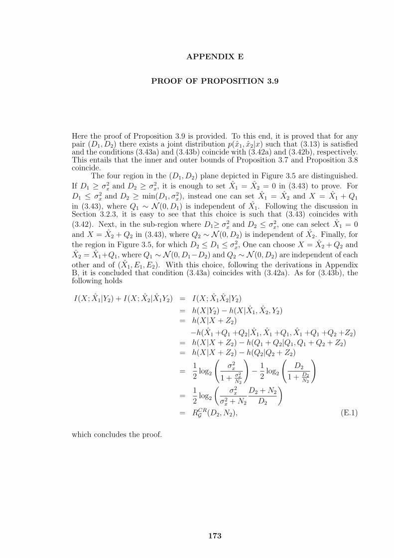
APPENDIX E
PROOF OF PROPOSITION 3.9
Here the proof of Proposition 3.9 is provided. To this end, it is proved that for anypair (D1, D2) there exists a joint distribution p(x1, x2|x) such that (3.13) is satisfiedand the conditions (3.43a) and (3.43b) coincide with (3.42a) and (3.42b), respectively.This entails that the inner and outer bounds of Proposition 3.7 and Proposition 3.8coincide.
The four region in the (D1, D2) plane depicted in Figure 3.5 are distinguished.
If D1 ≥ σ2x and D2 ≥ σ2
x, it is enough to set X1 = X2 = 0 in (3.43) to prove. For
D1 ≤ σ2x and D2 ≥ min(D1, σ
2x), instead one can set X1 = X2 and X = X1 + Q1
in (3.43), where Q1 ∼ N (0, D1) is independent of X1. Following the discussion inSection 3.2.3, it is easy to see that this choice is such that (3.43) coincides with
(3.42). Next, in the sub-region where D1≥ σ2x and D2 ≤ σ2
x, one can select X1 = 0
and X = X2 +Q2 in (3.43), where Q2 ∼ N (0, D2) is independent of X2. Finally, for
the region in Figure 3.5, for which D2 ≤ D1 ≤ σ2x, One can choose X = X2 +Q2 and
X2 = X1+Q1, where Q1 ∼ N (0, D1−D2) and Q2 ∼ N (0, D2) are independent of each
other and of (X1, E1, E2). With this choice, following the derivations in AppendixB, it is concluded that condition (3.43a) coincides with (3.42a). As for (3.43b), thefollowing holds
I(X; X1|Y2) + I(X; X2|X1Y2) = I(X; X1X2|Y2)= h(X|Y2)− h(X|X1, X2, Y2)= h(X|X + Z2)
−h(X1 +Q1 +Q2|X1, X1 +Q1, X1 +Q1 +Q2 +Z2)= h(X|X + Z2)− h(Q1 +Q2|Q1, Q1 +Q2 + Z2)= h(X|X + Z2)− h(Q2|Q2 + Z2)
=1
2log2
(σ2x
1 + σ2x
N2
)− 1
2log2
(D2
1 + D2
N2
)
=1
2log2
(σ2x
σ2x +N2
D2 +N2
D2
)= RCR
G (D2, N2), (E.1)
which concludes the proof.
173

APPENDIX F
PROOF OF PROPOSITION 3.10
Here the proof of Proposition 3.10 is provided. Following similar steps as in AppendixE, it is proved that for any pair (D1, D2) there exists a joint distribution p(x1, x2|x)such that (3.13) is satisfied and the conditions (3.43a) and (3.43b) coincide with(3.42a) and (3.42b), respectively. This entails that the inner and outer bounds ofProposition 3.7 and Proposition 3.8 coincide.
The four region in the (D1, D2) plane depicted in Figure 3.8 are distinguished.
If D1 ≥ 1/2 and D2 ≥ 1/2, it is enough to set X1 = X2 = 0 in (3.43) to prove the
desired result. For D1 ≤ 1/2 and D2 ≥ min(D1, 1/2), one can instead set X1 = X2
and X = X1⊕Q1 in (3.43), where Q1 ∼ Ber(D1) is independent of X1. Following thediscussion in Section 3.2.4, it is easy to see that this choice is such that (3.43) coincideswith (3.42). Next, in the sub-region where D1 ≥ 1/2 and D2 ≤ 1/2, one can select
X1 = 0 andX = X2⊕Q2 in (3.43), whereQ2 ∼ Ber(D2) is independent of X2. Finally,
for the region in Figure 3.8, for which D2 ≤ D1 ≤ 1/2, one can choose X = X2 ⊕Q2
and X2 = X1 ⊕Q1, where Q1 ∼ Ber(D1 ∗D2) and Q2 ∼ Ber(D2) are independent of
each other and of (X1, E1, E2). With this choice, following the derivations in AppendixD, it is concluded that condition (3.43a) coincides with (3.42a). As for (3.43b), thefollowing hold
I(X; X1X2|Y2) = H(X|Y2)−H(X|X1, X2, Y2)
= p2 − p2H(X|X1, X2, Y2 = X)− (1− p2)H(X|X1, X2, Y2 = X)
= p2 − p2H(X|X1, X2)(a)= p2 − p2H(X|X2)
= p2 − p2H(X2 ⊕Q2|X2)= p2 − p2H(D2)
= RCRB (D2, p2), (F.1)
where (a) follows by the Markov chain relationship X− X2− X1. This completes theproof.
174

APPENDIX G
PROOF OF PROPOSITION 3.11
The proof of the achievability follows from standard arguments, similar to [3]. Forthe converse, following the proof of [3, Theorem 3] It is true that for any (R,De,1 +ϵ,De,2 + ϵ,D1 + ϵ,D2 + ϵ) code, the following inequality holds:
nR ≥n∑
i=1
I(Xi;U1i|Y1i) + I(Xi;U2i|Y2i), (G.1)
with the definitions Uji△= (J, Y
n\ij ), for j = 1, 2, with Y
n\ij = [Y i−1
j1 , Y nj(i+1)]. Note that
with the given definition of Uji, the ith element of the decoding functions (3.5)-(3.6)can be written as hji(J, Y
nj ) = xji(Uji, Yji) for all i = 1, ..., n and j = 1, 2. Now,
defining De,ji△= E[de,j(h
nji(M,Y n
j ), ψji(Xn)], The following chain of inequalities for
the code at hand and j = 1, 2 hold:
De,ji = EXnY nj[de,j(h
nji(J, Y
nj ), ψji(X
n))] (G.2a)
(a)= EXnUjiYji
[de,j(xji(Uji, Yji), ψji(Xn))] (G.2b)
= EXnUjiEYji
[de,j(xji(Uji, Yji), ψji(Xi, Xn\i))|XnUji] (G.2c)
=n∑
xn∈Xn,uji∈U
p(xn, uji) (G.2d)
EYji[de,j(xji(Uji, Yji), ψji(Xi, X
n\i))|Xi = xi, Xn\i = xn\i, Uji = uji]
(b)
≥n∑
xn∈Xn,uji∈U
p(xn, uji) (G.2e)
EYji[de,j(xji(Uji, Yji), ψji(Xi, X
n\i))|Xi = xi, Xn\i = x∗n\i(xi, uji), Uji = uji]
(c)=
n∑xn∈Xn,uji∈U
p(xn, uji) (G.2f)
EYji[de,j(xji(Uji, Yji), xe,ji(Uji, Xi))|Xi = xi, Uji = uji]
= EXiUjiYji[de,j(xji(Uji, Yji), xe,ji(Uji, Xi))], (G.2g)
where (a) follows by using the definition of random variables Uj = (J, Yn\ij ); (b)
follows by selecting x∗n\i(xi, uji) as
x∗n\i(xi, uji) ∈ argminxn\i∈Xn\i
EYji[de,j(xji(Uji, Yji), ψji(Xi, X
n\ii ))|Xi = xi, X
n\i = xn\i, Uji = uji];
175

176
and (c) follows from the Markov chain relationship Yji−(Xi, Uji)−Xn\i and from thedefinition xe,ji(Uji, Xi) = ψji(Xi, x
∗n\i(Xi, Uji)). Let Q be a uniform random variable
over the interval [1, n] and independent of the variables (Xn, Y n1 , Y
n2 , U
n1 , U
n2 , X
n1 , X
n2
, Xne,1, X
ne,2) and define the random variables Uj
△= (Q,UjQ), X
△= XQ, Yj
△= YjQ, Xj
△=
XjQ, and Xe,j△= Xe,jQ for j = 1, 2. Moreover, note that Xj is a deterministic function
of Uji and Yji, and Xe,j is a deterministic function of Uji andXi for j = 1, 2. The proofis completed by using (3.45) and the fact that the term I(Xi;U1i|Y1i) + I(Xi;U2i|Y2i)in (G.1) is convex with respect to the pmf p(u1i, u2i|xi), using standard steps (see,e.g., [13]).

APPENDIX H
CARDINALITY BOUNDS
Using standard inequalities, it can be seen that the rate region (4.12) evaluated witha constant Q is a contra-polymatroid, as the Berger-Tung region (4.17) (see e.g., [69]).Moreover, the role of the variable Q is that of performing the convexification of theunion of all regions of tuples (R1, R2, D1, D2,Γ) that satisfy (4.12) and (4.14) for somefixed Q. It follows from [69] that every extreme point of region of achievable tuples(R1, R2, D1, D2,Γ) satisfies the equations
R1 = I(X1;V1|V2) + I(X1;U1|U2, V1, V2, Y ) (H.1a)R2 = I(X2;V2) + I(X2;U2|V1, V2, Y ) (H.1b)
along with (4.14), where both relationships are satisfied with equality, or
R1 = I(X1;V1) + I(X1;U1|V1, V2, Y ) (H.2a)R2 = I(X2;V2|V1) + I(X2;U2|U1, V1, V2, Y ) (H.2b)
along with (4.14) satisfied with equality. Applying the Fenchel–Eggleston–Caratheodorytheorem to the right-hand side of the equations above and to (4.14) concludes theproof (See [1, Appendix C] and [29]).
177

APPENDIX I
PROOF OF THE CONVERSE FOR PROPOSITION 4.3
In this section, the proof of converse for Proposition 4.3 is given. For any(n,R1, R2, D1 + ϵ,D2 + ϵ,Γ + ϵ) code, the following inequalities hold
nR1 ≥ H(M1) ≥ H(M1|M2)(a)= I(M1;X
n1 , X
n2 |M2)
=n∑
i=1
H(X1i, X2i|X i−11 , X i−1
2 ,M2)−H(X1i, X2i|X i−11 , X i−1
2 ,M1,M2)
(b)=
n∑i=1
H(X1i, X2i|X i−11 , X i−1
2 ,M2)−H(X1i, X2i|X i−11 , X i−1
2 ,M1,M2, Yi−1)
(c)
≥n∑
i=1
H(X1i, X2i|X i−11 , X i−1
2 ,M2, Yi−1)−H(X1i, X2i|X i−1
1 , X i−12 ,M1,M2, Y
i−1)
(d)=
n∑i=1
I(X1i, X2i;U1i|U2i),
where (a) follows because M1 is a function of (Xn1 , X
n2 ) given that Xn
2 is a functionof Xn
1 by assumption; (b) follows since (X1i, X2i)—(X i−11 , X i−1
2 ,M1,M2)—Y i−1formsa Markov chain; (c) follows by the fact that conditioning decreases entropy; and (d)follows by defining Uji = (X i−1
1 , X i−12 , Y i−1,Mj) for j = 1, 2. A similar chain of
inequalities hold for R2. As for the sum-rate R1 +R2, it is true that
n(R1 +R2) ≥ H(M1,M2)(a)= I(M1,M2;X
n1 , X
n2 )
=n∑
i=1
H(X1i, X2i|X i−11 , X i−1
2 )−H(X1i, X2i|X i−11 , X i−1
2 ,M1,M2)
(b)=
n∑i=1
H(X1i, X2i|X i−11 , X i−1
2 )−H(X1i, X2i|X i−11 , X i−1
2 ,M1,M2, Yi−1)
(c)
≥n∑
i=1
I(X1i, X2i;U1i, U2i),
where (a) follows because (M1,M2) are functions of (Xn1 , X
n2 ); (b) follows since
(X1i, X2i)— (X i−11 , X i−1
2 ,M1,M2)—Y i−1 forms a Markov chain; and (c) follows using
178
179
the definition of Uji for j = 1, 2. Next, let Q be a uniform random variable over the
interval [1, n] and independent of (Xn1 , X
n2 , U
n1 , U
n2 , Y
n) and define Uj∆= (Q,UjQ), for
j = 1, 2, X1∆= X1Q, X2
∆= X2Q, Y
∆= YQ. Note that Xj is a function of U1, U2 and Y
for j = 1, 2. Moreover, from (4.8) and (7.7), it holds that
Γ + ϵ ≥ 1
n
n∑i=1
E [Λ(Ai)] = E[Λ(A)] (I.1)
and Dj + ϵ ≥ 1
n
n∑i=1
E[dj(X1i, X2i, Yi.Xji, )
]= E[d1(X1, X2, Y, Xj)], for j = 1, 2.
(I.2)
APPENDIX J
PROOF OF THE CONVERSE FOR PROPOSITION 4.4
In this section, the proof of converse for Proposition 4.4 is given. Fix a code(n,R1, R2, D1 + ϵ, ϵ,Γ) for an ϵ > 0, whose existence for all sufficiently large n isrequired by the definition of achievability.
From the distortion constraint for X2, the following inequality holds
ϵ ≥ 1
n
n∑i=1
E[dH(X2i, X2i)](a)=
1
n
n∑i=1
pe,2i, (J.1)
where the definition pe,2i = Pr[X2i = X2i] is used, and (a) follows from the definitionof the metric dH(x, x) as the Hamming distortion. Moreover, the following chain ofinequalities hold
H(Xn2 |Xn
2 )(a)
≤n∑
i=1
H(X2i|X2i)(b)
≤n∑
i=1
H(pe,i) + pe,i log∣∣∣X2i
∣∣∣(c)
≤ nH
(1
n
n∑i=1
pe,i
)+ n
(1
n
n∑i=1
pe,i
)log∣∣∣X2i
∣∣∣(d)
≤ nH(ϵ) + nϵ log∣∣∣Xji
∣∣∣∆= nδ(ϵ), (J.2)
where (a) follows by conditioning reduces entropy; (b) follows by Fano’s inequality;(c) follows by Jensen’s inequality; and (d) follows by (J.1), where δ(ϵ) → 0 as ϵ→ 0.Note that, in the following, the convention in [1, Chapter 3] of defining as δ(ϵ) anyfunction such that δ(ϵ) → 0 as ϵ→ 0 is used.
For rate R1, then the following series of inequalities hold
nR1 ≥ H(M1)(a)= H(M1, A
n)
= H(An) +H(M1|An)(b)
≥ H(An)−H(An|Xn1 , X
n2 ) +H(M1|An, Y n, Xn
2 )−H(M1|An, Y n, Xn1 , X
n2 )
= I(An;Xn1 , X
n2 ) + I(M1;X
n1 |An, Y n, Xn
2 )
= I(An;Xn1 , X
n2 ) +H(Xn
1 |An, Y n, Xn2 )−H(Xn
1 |An, Y n, Xn2 ,M1)
= H(Xn1 , X
n2 )−H(Xn
1 , Xn2 |An) +H(Xn
1 , Xn2 , Y
n|An)−H(Y n, Xn2 |An)
−H(Xn1 |An, Y n, Xn
2 ,M1)
= H(Xn1 , X
n2 ) +H(Y n|An, Xn
1 , Xn2 )−H(Y n, Xn
2 |An)
−H(Xn1 |An, Y n, Xn
2 ,M1), (J.3)
180

181
where (a) follows because An is a function of M1 and (b) follows because entropy isnon-negative and conditioning decreases entropy. For the first three terms in (J.3) itis also true that
H(Xn1 , X
n2 ) +H(Y n|An, Xn
1 , Xn2 )−H(Y n, Xn
2 |An)
= H(Xn1 , X
n2 ) +H(Y n|An, Xn
1 , Xn2 )−H(Y n|An)−H(Xn
2 |An, Y n)
(a)=
n∑i=1
H(X1i, X2i) +H(Yi|Y i−1, An, Xn1 , X
n2 )−H(Yi|Y i−1, An)−H(X2i|X i−1
2 , An, Y n)
(b)
≥n∑
i=1
H(X1i, X2i) +H(Yi|Ai, X1i, X2i)−H(Yi|Ai)−H(X2i|Ai, Yi)
=n∑
i=1
H(X1i, X2i)− I(Yi;X1i, X2i|Ai)−H(X2i|Ai, Yi)
=n∑
i=1
H(X1i, X2i)−H(X1i, X2i|Ai) +H(X1i, X2i|Ai, Yi)−H(X2i|Ai, Yi)
=n∑
i=1
I(X1i, X2i;Ai) +H(X1i|Ai, Yi, X2i), (J.4)
where (a) follows by the chain rule for entropy and the fact that Xn1 , X
n2 are i.i.d. and
(b) follows since Yi—(Ai, X1i, X2i)—(Y i−1, An\i, Xn\i1 , X
n\i2 ) forms a Markov chain, by
the definition of problem, and since conditioning reduces entropy.
Combining (J.3) and (J.4), and defining U1i = (An\i, Y n\i, Xn\i2 ,M1), it holds
that
nR1
(a)
≥n∑
i=1
I(X1i, X2i;Ai) +H(X1i|Ai, Yi, X2i)
−H(X1i|X i−11 , An, Y n, Xn
2 ,M1)
(b)
≥n∑
i=1
I(X1i;Ai) +H(X1i|Ai, Yi, X2i)−H(X1i|An, Y n, Xn2 ,M1)
(c)=
n∑i=1
(X1i;Ai) + I(X1i;U1i|Ai, Yi, X2i), (J.5)
where (a) follows by the chain rule for entropy; (b) follows because mutual informationis non-negative and due to the fact that conditioning decreases entropy; and (c)follows by the definition of mutual information and definition of U1i.

182
Next, the rate R2 is considered.
nR2 ≥ H(M2) ≥ H(M2|An, Y n,M1)−H(M2|An, Y n,M1, Xn2 )
= I(M2;Xn2 |An, Y n,M1)
= H(Xn2 |An, Y n,M1)−H(Xn
2 |An, Y n,M1,M2)(a)
≥ H(Xn2 |An, Y n,M1)− nδ(ϵ)
=n∑
i=1
H(X2i|X i−12 , An, Y n,M1)− nδ(ϵ)
(b)
≥n∑
i=1
H(X2i|Ai, Yi, U1i)− nδ(ϵ), (J.6)
where (a) follows because from (J.2), H(Xn2 |An, Y n,M1,M2) ≤ H(Xn
2 |Xn2 ) ≤ nδ(ϵ),
given that Xn2 is a function of M1, M2 and Y nand (b) follows using the definition of
U1i and due to the fact that conditioning decreases entropy. For the sum-rate R1+R2,also the following series of inequalities hold
n(R1 +R2) ≥ H(M1,M2)(a)= H(M1,M2, A
n)
= H(An) +H(M1,M2|An)
≥ H(An)−H(An|Xn1 , X
n2 ) +H(M1,M2|An, Y n)
−H(M1,M2|An, Y n, Xn1 , X
n2 )
= I(An;Xn1 , X
n2 ) + I(M1,M2;X
n1 , X
n2 |An, Y n)
= I(An;Xn1 , X
n2 ) +H(Xn
1 , Xn2 |An, Y n)−H(Xn
1 , Xn2 |An, Y n,M1,M2)
= H(Xn1 , X
n2 )−H(Xn
1 , Xn2 |An) +H(Xn
1 , Xn2 , Y
n|An)−H(Y n|An)
−H(Xn2 |An, Y n,M1,M2)−H(Xn
1 |An, Y n, Xn2 ,M1,M2)
(b)
≥ H(Xn1 , X
n2 ) +H(Y n|An, Xn
1 , Xn2 )−H(Y n|An)
−H(Xn1 |An, Y n, Xn
2 ,M1,M2)− nδ(ϵ), (J.7)

183
where (a) follows because An is a function of M1; and (b) follows as in (a) of (J.6).For the first three terms in (J.7), it is true that
H(Xn1 , X
n2 ) +H(Y n|An, Xn
1 , Xn2 )−H(Y n|An)
(a)=
n∑i=1
H(X1i, X2i) +H(Yi|Y i−1, An, Xn1 , X
n2 )−H(Yi|Y i−1, An)
(b)
≥n∑
i=1
H(X1i, X2i) +H(Yi|Ai, X1i, X2i)−H(Yi|Ai)
=n∑
i=1
H(X1i, X2i)− I(Yi;X1i, X2i|Ai)
=n∑
i=1
H(X1i, X2i)−H(X1i, X2i|Ai) +H(X1i, X2i|Ai, Yi)
=n∑
i=1
I(X1i, X2i;Ai) +H(X2i|Ai, Yi) +H(X1i|Ai, Yi, X2i), (J.8)
where (a) follows from the chain rule for entropy and by the chain rule for entropyand the fact that (Xn
1 , Xn2 ) are i.i.d.; and (b) follows since Yi—(Ai, X{1,2}i)—
(Y i−1, An\i, Xn\i1 , X
n\i2 ) forms a Markov chain, by the definition of problem, and since
conditioning reduces entropy. Combining (J.7) and (J.8), and using the definition ofU1i, it holds that
n(R1 +R2)(a)
≥n∑
i=1
I(X1i, X2i;Ai) +H(X2i|Ai, Yi) +H(X1i|Ai, Yi, X2i)
−H(X1i|X i−11 , An, Y n, Xn
2 ,M1,M2)− nδ(ϵ)
(b)
≥n∑
i=1
I(X1i;Ai) +H(X2i|Ai, Yi) +H(X1i|Ai, Yi, X2i)
−H(X1i|An, Y n, Xn2 ,M1)− nδ(ϵ)
(c)
≥n∑
i=1
(X1i;Ai) +H(X2i|Ai, Yi) + I(X1i;U1i|Ai, Yi, X2i)− nδ(ϵ), (J.9)
where (a) follows by the chain rule for entropy; (b) follows because mutual informationis non-negative and due to the fact that conditioning decreases entropy; and (c)follows by the definition of mutual information and definition of U1i and the fact thatconditioning decreases entropy.
Moreover, (X2i, Yi)− (X1i, Ai)−U1i forms a Markov chain. This can be seen byusing the principle of d-separation [70, Section A.9] from Figure J.1, which representsthe joint distribution of all the variables at hand.
Let Q be a uniform random variable over the interval [1, n] and independent of
(Xn1 , X
n2 , A
n, Un1 , Y
n, Xn1 ) and define U1
∆= (Q,U1Q), X1
∆= X1Q, X2
∆= X2Q, Y
∆= YQ,
A∆= AQ, and X1
∆= X1Q. Note that X1 is a function of U1, X2 and Y . Moreover, from

184
1
1
-i
X
iX1
n
iX
)1+(1
1
2
-i
X
iX2
n
iX
)1+(2
1-iY
iY
n
iY 1+
1-iA
iA
n
iA
1+
1M
Figure J.1 Bayesian network representing the joint pmf of variables(M1, X
n1 , X
n2 , A
n, Y n) for the model in Figure 4.2.
(4.8) and (7.7), the following holds
Γ + ϵ ≥ 1
n
n∑i=1
E [Λ(Ai)] = E[Λ(A)]
and D1 + ϵ ≥ 1
n
n∑i=1
E[d1(X1i, X2i, Yi.X1i)
]= E[d1(X1, X2, Y, X1)]. (J.10)
Finally, since (J.5), (J.6) and (J.9) are convex with respect to p(a, u1|x1, q) forfixed p(q), p(x1, x2), and p(y|a, x1, x2), inequalities (4.20) hold, which completes theproof of (4.20a)-(4.22b). The cardinality bounds are proved by using the Fenchel–Eggleston–Caratheodory theorem in the standard way.

APPENDIX K
GREEDY ACTIONS ARE OPTIMAL WITH SUM SIDE
INFORMATION
Here, the equality below is proved.
R⊕sum, greedy(Γ) = R⊕
sum(Γ). (K.1)
which shows that no gain is accrued by choosing the actions based only on messageM1 with the sum side information. Fix the pmf p(a|x1) that achieves the minimumin the sum-rate obtained from (4.20c), namely
R⊕sum(Γ) = min I(X1;A) +H(X1, X2|A, Y ),
where the mutual information is calculated with respect to the distribution
p(x1, x2, y, a) = p(x1, x2)p(a|x1)p(y|a, x1, x2), (K.2)
and the minimum is taken over all distributions p(a|x1) such that E [Λ(A)] = E [A] ≤Γ. Note that for such a pmf p(a|x1), it is true that E[A] = p(a) = Γ, as it can beeasily seen. Next, following series of equalities hold
R⊕sum, greedy(Γ)−R⊕
sum(Γ)
(a)= ΓH(X1, X2|X1 ⊕X2) + (1− Γ)H(X1, X2)
−H(X1, X2|A,X1 ⊕X2)− I(X1;A)(b)= ΓH(X1|X1 ⊕X2) + (1− Γ)(1 +H(p))− ΓH(X1, X2|A = 1, X1 ⊕X2)
− (1− Γ)H(X1, X2|A = 0)− I(X1;A)(c)= ΓH(X1) + (1− Γ)(1 +H(p))− ΓH(X1|A = 1)− (1− Γ)H(X1|A = 0)
− (1− Γ)H(X2|X1, A = 0)− I(X1;A)(d)= Γ + (1− Γ)(1 +H(p))−H(X1|A)− (1− Γ)H(X2|X1)− I(X1;A)
= Γ + (1− Γ)(1 +H(p))−H(X1|A)− (1− Γ)H(p)− 1 +H(X1|A) = 0,
where (a) follows by the definition (4.27); (b) follows using the chain rule for entropyand from the definition of conditional entropy; (c) follows by the crypto-lemma [37,Lemma 2]; (d) follows from the fact that X2 −X1 − A forms a Markov chain.
185

APPENDIX L
PROOF OF THE CONVERSE FOR PROPOSITION 4.5
In this section, the proof of converse for Proposition 4.5 is provided. For any(n,R12, R23, D1 + ϵ,D2 + ϵ,Γ + ϵ) code, the following inequalities hold:
nR12 ≥ H(M12) ≥ H(M12|Xn2 )
(a)= H(M12,M23|Xn
2 )(b)= I(Xn
1 ;M12,M23|Xn2 )
=n∑
i=1
H(X1i|X i−11 , Xn
2 )−H(X1i|X i−11 , Xn
2 ,M12,M23)
(c)=
n∑i=1
H(X1i|X2i)−H(X1i|X i−11 , Xn
2 , An,M12,M23)
(d)=
n∑i=1
H(X1i|X2i)−H(X1i|X i−11 , Xn
2 , Yi−1,M12,M23, A
n, Xn1 )
(e)
≥n∑
i=1
H(X1i|X2i)−H(X1i|X2i, Ai, Ui, X1i)
=n∑
i=1
I(X1i;Ai, Ui, X1i|X2i), (L.1)
where (a) follows because M23 is a function of (M12,Xn2 ); (b) follows by definition of
mutual information and since M12 and M23 are functions of Xn1 and Xn
2 ; (c) followsbecause Xn
1 and Xn2 are i.i.d and since An is a function of M23; (d) follows because
Y i−1−(X i−11 , Xn
2 , An,M12,M23)−X1i forms a Markov chain and since Xn
1 is a functionof M12 and Xn
2 ; and (e) follows by defining Ui = (X i−11 , X i−1
2 , Y i−1, An\i,M23) andsince conditioning decreases entropy.
186

187
It is also true that
nR23 ≥ H(M23)(a)= I(Xn
1 , Xn2 ;M23)
(b)=
n∑i=1
H(X1i, X2i)−H(X1i, X2i|X i−11 , X i−1
2 ,M23)
(c)=
n∑i=1
H(X1i, X2i)−H(X1i, X2i|X i−11 , X i−1
2 , An,M23)
(d)=
n∑i=1
H(X1i, X2i)−H(X1i, X2i|X i−11 , X i−1
2 , Y i−1, An,M23)
(e)=
n∑i=1
H(X1i, X2i)−H(X1i, X2i|Ai, Ui)
=n∑
i=1
I(X1i, X2i;Ai, Ui), (L.2)
where (a) follows because M23 is a function of Xn1 and Xn
2 ; (b) follows by thedefinition of mutual information and the chain rule for entropy and since Xn
1 andXn
2 are i.i.d; (c) follows because An is a function of M23; (d) follows becauseY i−1 − (X i−1
1 , X i−12 , An,M23) − (X1i, X2i) forms a Markov chain; and (e) follows by
the definition of Ui.Let Q be a uniform random variable over [1, n] and independent of (Xn
1 , Xn2 , Y
n
, An, Un, Xn1 ) and define U
∆= (Q,UQ), X1
∆= X1Q, X2
∆= X2Q, Y
∆= YQ, A
∆= AQ,
X1∆= X1Q, and X2
∆= X2Q. Note that X2 is a function of U and Y . Moreover, from
(8.5) and (8.6), the following holds
Γ + ϵ ≥ 1
n
n∑i=1
E [Λ(Ai)] = E[Λ(A)] (L.3)
and Dj + ϵ ≥ 1
n
n∑i=1
E[dj(X1i, X2i, Yi, Xji)
]= E[dj(X1, X2, Y, Xj)] for j = 1, 2.
(L.4)
Finally, since (L.1) and (L.2) are convex with respect to p(a, u, x1|x1, x2)for fixed p(x1, x2) and p(y|a, x1, x2), from (L.1) and (L.2) it can be concludedthat inequalities (4.35) hold. The cardinality bounds are proved by using theFenchel-Eggleston-Caratheodory theorem in the standard way.
APPENDIX M
CONVERSE PROOF FOR PROPOSITION 5.1 AND 5.4
Here, the converse part of Proposition 5.4 is proved. Since the setting of Proposition5.1 is more restrictive, as it does not allow for adaptive actions, the converse proof forProposition 5.1 follows immediately. For any (n,R1, R2, D1 + ϵ,D2 + ϵ,Γ + ϵ) code,it is true that
nR1 ≥ H(M1)
≥ H(M1|Y n)(a)= I(M1;X
n, Zn|Y n)
= H(Xn, Zn|Y n)−H(Xn, Zn|M1, Yn)
= H(Xn|Y n) +H(Zn|Xn, Y n)−H(Zn|Y n,M1)−H(Xn|Zn, Y n,M1)(a,b)= H(Xn|Y n) +H(Zn|Xn, Y n,M1,M2)−H(Zn|Y n,M1,M2)
−H(Xn|Zn, Y n,M1,M2)(c)= H(Xn|Y n)−H(Xn|Zn, Y n,M1,M2, A
n, Xn1 )
+n∑
i=1
H(Zi|Zi−1, Xn, Y n,M1,M2)−H(Zi|Zi−1, Y n,M1,M2)
(c,d)
≥n∑
i=1
(H(Xi|Yi)−H(Xi|X i−1, Y i,M2, Ai, Zn, X1i))
+n∑
i=1
H(Zi|Zi−1, Xn, Y n,M1,M2, Ai)−H(Zi|Zi−1, Y n,M1,M2, Ai)
(e)=
n∑i=1
I(Xi; X1i, Ai, Ui|Yi) +H(Zi|Yi, Ai)−H(Zi|Yi, Ai)
=n∑
i=1
I(Xi; X1i, Ai, Ui|Yi), (M.1)
where (a) follows sinceM1 is a function of (Xn, Y n); (b) follows sinceM2 is a function
of (M1, Yn); (c) follows since Ai is a function of (M2, Z
i−1) and since Xn1 is a function
of (M1, Yn); (d) follows since conditioning decreases entropy and since Xn and Y n
are i.i.d.; and (e) follows by defining Ui = (M2, Xi−1, Y i−1, Ai−1, Zn\i) and since
(Zi−1, Xn, Y n\i,M1,M2)— (Ai, Yi)—Zi form a Markov chain by construction. It isalso true that
nR2 ≥ H(M2)= I(M2;X
n, Y n, Zn)
188

189
= H(Xn, Y n, Zn)−H(Xn, Y n, Zn|M2)= H(Xn, Y n) +H(Zn|Xn, Y n)−H(Zn|M2)−H(Xn, Y n|M2, Z
n)
=n∑
i=1
H(Xi, Yi) +H(Zi|Zi−1, Xn, Y n)−H(Zi|Zi−1,M2)
−H(Xi, Yi|X i−1, Y i−1,M2, Zn)
(a)=
n∑i=1
H(Xi, Yi)+H(Zi|Z i−1, Xn, Y n,M2, Ai)−H(Zi|Zi−1,M2, Ai)
−H(Xi, Yi|X i−1, Y i−1,M2, Zn, Ai)
(b)
≥n∑
i=1
H(Xi, Yi) +H(Zi|Xi, Yi, Ai)−H(Zi|Ai)−H(Xi, Yi|Ui, Ai, Zi), (M.2)
where (a) follows because M2 is a function of (M1, Yn) and thus of (Xn, Y n) and
because Ai is a function of (M2, Zi−1) and (b) follows since conditioning decreases
entropy, since the Markov chain relationship Zi—(Xi, Yi, Ai)— (Xn\i, Y n\i,M2) holdsand by using the definition of Ui.
Defining Q to be a random variable uniformly distributed over [1, n] and
independent of all the other random variables and with X△= XQ, Y
△= YQ, Z
△= ZQ,
A△= AQ, X1
△= X1Q, X2
△= X2Q and U
△= (UQ, Q), from (M.1), the following holds
nR1 ≥ I(X; X1, A, U |Y,Q)(a)
≥ H(X|Y )−H(X|X1, A, U, Y ) = I(X; X1, A, U |Y ),
where in (a) follows due to the fact that (Xn, Y n) are i.i.d and conditioning reducesentropy. Moreover, from (M.2) it follows that
nR2 ≥ H(X, Y |Q) +H(Z|X, Y,A,Q)−H(Z|A,Q)−H(X,Y |U,A, Z,Q)(a)
≥ H(XY ) +H(Z|X,Y,A)−H(Z|A)−H(X, Y |U,A,Z)= I(XY ;U,A, Z)− I(Z;X, Y |A)= I(XY ;A) + I(X, Y ;U |A,Z),
where (a) follows since (Xn, Y n) are i.i.d, since conditioning decreases entropy, by thedefinition of U and by the problem definition. It is noted that the defined randomvariables factorize as (8.8) since the Markov chain relationship X—(A, Y )—Z holds
by the problem definition and that X2 is a function f(U,Z) of U and Z by the definitionof U . Moreover, from the cost and distortion constraints (8.5)-(8.6), it is true that
Dj + ϵ ≥ 1
n
n∑i=1
E[dj(Xi, Xji)] = E[dj(X, Xj)], for j = 1, 2, (M.3a)
and Γ + ϵ ≥ 1
n
n∑i=1
E [Λ(Ai)] = E [Λ(A)] . (M.3b)

190
To bound the cardinality of auxiliary random variable U , p(z|y, a) is fixed andthe joint pmf p(x, y, z, a, u, x1) is factorized as
p(x, y, z, a, u, x1) = p(u)p(x1, a, x, y|u)p(z|y, a).
Therefore, for fixed p(z|y, a), the quantities (8.39a)-(8.9b) can be expressed in terms ofintegrals given by
´gj(p(x1, a, x, y|u))dF (u), for j = 1, ..., |X ||Y||A|+ 3, of functions
gj(·) that are continuous on the space of probabilities over alphabet X ×Y ×A×X1.Specifically, gj for j = 1, ..., |X ||Y||A| − 1, are given by the pmf p(a, x, y) for all
values of x ∈ X , y ∈ Y and a ∈ A, (except one), g|X ||Y||A| = H(X|A, Y, X1, U = u),
g|X ||Y||A|+1 = H(X, Y |A,Z, U = u), and g|X ||Y||A|+1+j = E[dj(X, Xj)|U = u], forj = 1, 2. The proof in concluded by invoking the Fenchel–Eggleston–Caratheodorytheorem [1, Appendix C].

APPENDIX N
PROOF OF PROPOSITION 5.3
Here, the converse parts of Proposition 5.3 and Proposition 5.5 are proved. Let’s startby proving Proposition 5.3. The proof of Proposition 5.5 will follow by setting Z = ∅,and noting that in the proof below the action Ai can be made to be a function ofY i−1, in addition to being a function ofMb, without modifying any steps of the proof.By the CR requirements (5.26), first it is observed that for any (n,R1, R2, Rb, D1 +ϵ,D2 + ϵ,Γ + ϵ) code, the Fano inequalities below hold
H(ψ1(Xn)|h1(M1,Mb, Y
n)) ≤ nδ(ϵ), (N.1a)and H(ψ2(X
n)|h2(M2,Mb, Zn)) ≤ nδ(ϵ), (N.1b)
where δ(ϵ) denotes any function such that δ(ϵ) → 0 if ϵ → 0. Next, it is also truethat
nRb ≥ H(Mb)(a)= I(Mb;X
n, Y n)
= H(Xn, Y n)−H(Xn, Y n|Mb)(a)= H(Xn) +H(Y n|Xn,Mb)−H(Xn, Y n|Mb)
(b)=
n∑i=1
H(Xi) +H(Yi|Y i−1, Xn,Mb, Ai)−H(Xi, Yi|X i−1, Y i−1,Mb, Ai)
=n∑
i=1
H(Xi) +H(Yi|Y i−1, Xn,Mb, Ai)−H(Xi|X i−1, Y i−1,Mb, Ai)
−H(Yi|X i, Y i−1,Mb, Ai)
(c)=
n∑i=1
H(Xi) +H(Yi|Xi, Ai)−H(Xi|X i−1, Y i−1,Mb, Ai)−H(Yi|Xi, Ai)
(d)
≥n∑
i=1
H(Xi)−H(Xi|Ai), (N.2)
where (a) follows since Mb is a function of Xn; (b) follows since Ai is a functionof Mb and since Xn is i.i.d.; (c) follows since (Y i−1, Xn\i,Mb)—(Ai, Xi)—Yi forms aMarkov chain by problem definition; and (d) follows conditioning reduces entropy.In the following, for simplicity of notation, h1, h2, ψ1, ψ2 is used for the values of
191

192
corresponding functions in Section 5.3.4. Next, the following holds
n(R1 +Rb)
≥ H(M1,Mb)(a)= I(M1,Mb;X
n, Y n, Zn)
= H(Xn, Y n, Zn)−H(Xn, Y n, Zn|M1,Mb)
= H(Xn) +H(Y n, Zn|Xn)−H(Y n, Zn|M1,Mb)−H(Xn|Y n, Zn,M1,Mb)(b)= H(Xn) +H(Y n, Zn|Xn,Mb)−H(Y n|M1,Mb)
−H(Zn|M1,Mb, Yn, An)−H(Xn|Y n, Zn,M1,Mb,M2, A
n)
(b,c)=
n∑i=1
H(Xi) +H(Yi, Zi|Xi, Ai)−H(Yi|Y i−1,M1,Mb, Ai)
−H(Zi|Zi−1,M1,Mb, Yn, An)−H(Xi|X i−1, Y n, Zn,M1,Mb, A
n,M2, h1, h2)
(d)
≥n∑
i=1
H(Xi)+H(Yi|Xi, Ai) +H(Zi|Yi, Ai)−H(Yi|Ai)−H(Zi|Yi, Ai)
−H(Xi|Yi, Ai, h1, h2)n∑
i=1
I(Xi;Yi, Ai, h1, h2)− I(Yi;Xi|Ai)
n∑i=1
I(Xi;Yi, Ai, h1, h2, ψ1, ψ2)− I(Xi;ψ1, ψ2|Yi, Ai, h1, h2)− I(Yi;Xi|Ai)
(e)
≥n∑
i=1
I(Xi;Yi, Ai, ψ1, ψ2)−H(ψ1, ψ2|Yi, Ai, h1, h2)
+H(ψ1, ψ2|Yi, Ai, h1, h2, Xi)− I(Yi;Xi|Ai)
(f)
≥n∑
i=1
I(Xi;Yi, Ai, ψ1, ψ2)− I(Yi;Xi|Ai) + nδ(ϵ)
=n∑
i=1
I(Xi;Ai) + I(Xi;ψ1, ψ2|Yi, Ai) + nδ(ϵ), (N.3)
where (a) follows because (M1,Mb) is a function of Xn; (b) follows because Mb
is a function of Xn, An is a function of Mb and M2 is a function of (M1,Mb, Yn);
(c) follows since H(Y n, Zn|Xn,Mb) =∑n
i=1H(Yi, Zi| Y i−1, Z i−1, Xn,Mb, Ai) =∑ni=1H(Yi, Zi|Xi, Ai) and since h1 and h2 are functions of (M1,Mb, Y
n) and (M2,Mb, Zn),
respectively and because (Yi, Zi)—(Xi, Ai)— (Xn\i, Y i−1, Z i−1,Mb) forms a Markovchain; (d) follows since conditioning reduces entropy, since side information VMfollows p(yn, zn|an, xn)=
∏ni=1 pY |A,X(yi|ai, xi) pZ|A,Y (zi|ai, yi) from (7.24) and because
Zi—(Yi, Ai)— (Y n\i, Zi−1,M1,Mb) forms a Markov chain; (e) follows by the chain rulefor mutual information and the fact that mutual information is non-negative; and (f)follows by the Fano inequality (R.2) and because entropy is non-negative. It holds
193
that
n(R2 +Rb) ≥ H(M2,Mb)(a)= I(M2,Mb;X
n, Y n, Zn)
= H(Xn, Y n, Zn)−H(Xn, Y n, Zn|M2,Mb)(a)= H(Xn) +H(Y n, Zn|Xn,Mb)−H(Zn|M2,Mb)
−H(Xn, Y n|Zn,M2,Mb)
(b)=
n∑i=1
H(Xi) +H(Yi, Zi|Y i−1, Z i−1, Xn,Mb, Ai)
−H(Zi|Zi−1,M2,Mb, Ai)−H(Xi, Yi|X i−1, Y i−1,M2,Mb, Zn, Ai)
=n∑
i=1
H(Xi, Yi)−H(Yi|Xi) +H(Yi, Zi|Y i−1, Z i−1, Xn,Mb, Ai)
−H(Zi|Zi−1,M2,Mb, Ai)−H(Xi, Yi|X i−1, Y i−1,M2,Mb, Zn, Ai)
(c)=
n∑i=1
H(Xi, Yi)−H(Yi|Xi) +H(Yi|Xi, Ai) +H(Zi|Ai, Yi, Xi)
−H(Zi|Zi−1,M2,Mb, Ai)−H(Xi, Yi|X i−1, Y i−1,M2,Mb, Zn, Ai)
(d)=
n∑i=1
H(Xi, Yi)− I(Yi;Ai|Xi) +H(Zi|Ai, Yi, Xi)
−H(Zi|Zi−1,M2,Mb, Ai)−H(Xi, Yi|X i−1, Y i−1,M2,Mb, h2, Zn, Ai)
(e)
≥n∑
i=1
H(Xi, Yi) + I(Xi;Ai)− I(Yi, Xi;Ai) +H(Zi|Ai, Yi, Xi)
−H(Zi|Ai)−H(Xi, Yi|h2, Ai, Zi)
=n∑
i=1
I(Xi, Yi; h2, Ai, Zi, ψ2i)− I(Xi, Yi;ψ2i|h2, Ai, Zi) + I(Xi;Ai)
− I(Yi, Xi;Ai)− I(Xi, Yi;Zi|Ai)
≥n∑
i=1
I(Xi, Yi;Ai, Zi, ψ2i)−H(ψ2i|h2, Ai, Zi) +H(ψ2i|h2, Ai, Xi, Yi, Zi)
+ I(Xi;Ai)− I(Xi, Yi;Zi, Ai)
(f)
≥n∑
i=1
I(Xi;Ai) + I(Xi, Yi;ψ2i|Ai, Zi) + nδ(ϵ), (N.4)
where (a) follows since Mb is a function of Xn and because M2 is a function of(M1,Mb, Y
n) and thus of (Xn, Y n); (b) follows since Ai is a function of Mb andsince Xn is i.i.d.; (c) follows since (Yi, Zi)—(Xi, Ai)— (Xn\i, Y i−1, Zi−1,Mb) formsa Markov chain and since p(yn, zn|an, xn) =
∏ni=1 pY |A,X(yi|ai, xi)pZ|A,Y (zi|ai, yi); (d)
follows since h2 is a function of (M2,Mb, Zn); (e) follows since conditioning reduces
entropy; and (f) follows since entropy is non-negative and using the Fanos inequality.Moreover, with the definition M = (M1,M2,Mb), the following chain of inequalities

194
hold
n(R1 +R2 +Rb) ≥ H(M)(a)= I(M ;Xn, Y n, Zn)
= H(Xn, Y n, Zn)−H(Xn, Y n, Zn|M)(a)= H(Xn) +H(Y n, Zn|Xn,Mb)−H(Xn, Y n, Zn|M)
= I(Xn;An) +H(Y n, Zn|Xn,Mb)−H(Y n, Zn|M)
−H(Xn|Y n, Zn,M) +H(Xn|An)
= I(Xn;An) +H(Y n, Zn|Xn,Mb)−H(Y n, Zn|M) + I(Xn;Y n, Zn,M |An)
= I(Xn;An) + I(M ;Xn|Y n, An, Zn) +H(Y n, Zn|Xn,Mb)
−H(Y n, Zn|M) + I(Xn;Y n, Zn|An)(b)= H(Xn)−H(Xn|An) +H(Xn|Y n, An, Zn)−H(Xn|Y n, An, Zn,M)
−H(Y n, Zn|M) +H(Y n, Zn|An)
= H(Xn)−H(Xn|An) +H(Xn, Y n, Zn|An)−H(Xn|Y n, An, Zn,M)
−H(Y n, Zn|M)
= H(Xn) +H(Y n, Zn|An, Xn)−H(Xn|Y n, An, Zn,M)−H(Y n, Zn|M)
(c)=
n∑i=1
H(Xi) +H(Yi|Ai, Xi) +H(Zi|Ai, Yi)−H(Xi|X i−1, Y n, An, Zn,M)
−H(Zi|Zi−1,M,Ai)−H(Yi|Y i−1, Zn,M,Ai)
(d)=
n∑i=1
H(Xi)+H(Yi|Ai, Xi)+H(Zi|Ai, Yi)−H(Xi|X i−1,Y n, An, Zn,M, h1, h2)
−H(Zi|Zi−1,M,Ai)−H(Yi|Y i−1, Zn,M,Ai, h2)
≥n∑
i=1
H(Xi) +H(Yi|Ai, Xi) +H(Zi|Ai, Yi)−H(Xi|Yi, Ai, h1, h2)
−H(Zi|Ai)−H(Yi|Zi, Ai, h2)(e)
≥ I(Xi;Ai, Yi, ψ1, ψ2) +H(Yi|Ai, Xi) +H(Zi|Ai, Yi)
−H(Zi|Ai)−H(Yi|Zi, Ai, ψ2)− nδ(ϵ), (N.5)
where (a) follows since (M1,Mb) is a function of Xn and M2 is a function of(M1,Mb, Y
n); (b) follows since H(Y n, Zn|Xn,Mb) =∑n
i=1H(Yi, Zi| Y i−1, Zi−1, Xn,Mb, Ai) =
∑ni=1H(Yi, Zi| Xi, Ai) = H(Y n, Zn|Xn, An); (c) follows since Ai is a
function of Mb; (d) follows since h1, h2 are functions of (M,Y n) and (M,Zn),respectively; and (e) follows since entropy is non-negative and by Fano’s inequality.Next, from (N.5) it is true that

195
n(R1 +R2 +Rb) ≥ I(Xi;Ai, Yi, ψ1, ψ2) +H(Yi|Ai, Xi) +H(Zi|Ai, Yi)−H(Zi|Ai)
−H(Yi, Zi|Ai, ψ2) +H(Zi|Ai, ψ2)− nδ(ϵ)
= I(Xi;Ai, Yi, ψ1, ψ2) +H(Yi|Ai, Xi)−H(Zi|Ai)−H(Yi|Ai, ψ2)
+H(Zi|Ai, ψ2)− nδ(ϵ)
= I(Xi;Ai, Yi, ψ1, ψ2)− I(Xi;Yi|Ai, ψ2)− I(Zi;ψ2|Ai)− nδ(ϵ)(a)= I(Xi;Ai, Yi, ψ1, ψ2)− I(Xi;Yi|Ai, ψ2)− I(Yi;Ai|Xi)− I(Zi;Yi|Ai)
+ I(Yi;Ai, ψ2|Xi) + I(Zi;Yi|ψ2, Ai)− nδ(ϵ)(b)= I(Xi;Ai, Yi, ψ1, ψ2)− I(Xi;Yi|Ai, ψ2) + I(Xi;Ai)− I(Yi, Xi;Ai)
− I(Zi;Xi, Yi|Ai) + I(Xi, Yi;Ai, ψ2) + I(Zi;Xi, Yi|ψ2, Ai)− I(Xi;Ai, ψ2)− nδ(ϵ)
= I(Xi;Ai) + I(Xi;Ai, Yi, ψ1, ψ2) + I(Xi, Yi;Ai, ψ2, Zi)− I(Ai, Zi;Xi, Yi)
− I(Xi;Yi, Ai, ψ2)− nδ(ϵ)
= I(Xi;Ai)+I(Xi;Ai, Yi, ψ1, ψ2) + I(Xi, Yi;ψ2|Ai, Zi)− I(Xi;Yi, Ai, ψ2)− nδ(ϵ)
= I(Xi;Ai) + I(Xi, Yi;ψ2|Ai, Zi) + I(Xi;ψ1|Ai, Yi, ψ2)− nδ(ϵ), (N.6)
where (a) is true since
I(Yi;Ai|Xi) + I(Zi;Yi|Ai)− I(Yi;Ai, ψ2|Xi)− I(Zi;Yi|ψ2, Ai)= H(Yi|Xi)−H(Yi|Xi, Ai) +H(Zi|Ai)−H(Zi|Ai, Yi)−H(Yi|Xi) +H(Yi|Xi, Ai)−H(Zi|ψ2, Ai) +H(Zi|Ai, Yi)= H(Zi|Ai)−H(Zi|ψ2, Ai);
(b) follows because I(Zi;Xi, Yi|Ai) = I(Zi;Yi|Ai) and I(Zi;Xi, Yi|Ai, ψ2) = I(Zi;Yi|Ai, ψ2).
Next, define Xji = ψji(Xn) for j = 1, 2 and i = 1, 2, ..., n and let Q be a random
variable uniformly distributed over [1, n] and independent of all the other random
variables and with X△= XQ, Y
△= YQ, A
△= AQ, from (N.2), it holds that
nRb ≥ H(X|Q)−H(X|A,Q)(a)
≥ H(X)−H(X|A) = I(X;A),
where (a) follows since Xn is i.i.d. and since conditioning decreases entropy. Next,from (N.3), the following holds
n(R1 +Rb) ≥ I(X;A|Q) + I(X; X1, X2|Y,A,Q)(a)
≥ I(X;A) + I(X; X1, X2|Y,A),

196
where (a) follows since Xn is i.i.d., since conditioning decreases entropy and by theproblem definition. From (N.4), it is also true that
n(R2 +Rb) ≥ I(X;A|Q) + I(X, Y ; X2|A,Z,Q)(a)
≥ I(X;A) +H(X,Y |A,Z,Q)−H(X,Y |A,Z, X2)(b)= I(X;A) +H(Y |A,Z) +H(X|A, Y, Z)−H(X, Y |A,Z, X2)
= I(X;A) + I(X,Y ; X2|A,Z)≥ I(X;A) + I(X; X2|A,Z)
where (a) follows since Xn is i.i.d. and by conditioning reduces entropy; and (b)follows by the problem definition. Finally, from (N.6), the following holds
n(R1 +R2 +Rb) ≥ I(X,A|Q) + I(X,Y ; X2|A,Z,Q) + I(X; X1|A, Y, X2, Q)(a)
≥ I(X,A) +H(X,Y |A,Z,Q)−H(X,Y |A,Z, X2) + I(X; X1|A, Y, X2)(b)= I(X;A)+H(Y |A,Z)+H(X|A, Y, Z)−H(X,Y |A,Z, X2)+I(X; X1|A, Y, X2)
= I(X;A) + I(X, Y ; X2|A,Z) + I(X; X1|A, Y, X2)
≥ I(X;A) + I(X; X2|A,Z) + I(X; X1|A, Y, X2) (N.7)
where (a) follows since Xn is i.i.d, since conditioning decreases entropy, and by theproblem definition; and (b) follows by the problem definition. From cost constraint(8.5), it holds
Γ + ϵ ≥ 1
n
n∑i=1
E [Λ(Ai)] = E [Λ(A)] . (N.8)
Moreover, let B be the event B = {(ψ1(Xn) = h1(M1,Mb, Y
n)) ∧ (ψ2(Xn) =
h2(M2,Mb))}. Using the CR requirement (5.26), Pr(B) ≤ ϵ. For j = 1, 2, it is truethat
E[d(Xj, Xj)
]=
1
n
n∑i=1
E[d(Xji, Xji)
]=
1
n
n∑i=1
E[d(Xji, Xji)
∣∣∣B]Pr(B)+1
n
n∑i=1
E[d(Xji, Xji)
∣∣∣Bc]Pr(Bc)
(a)
≤ 1
n
n∑i=1
E[d(Xji, Xji)
∣∣∣Bc]Pr(Bc) + ϵDmax
(b)
≤ 1
n
n∑i=1
E [d(Xji, hji)] + ϵDmax
(c)
≤ Dj + ϵDmax, (N.9)

197
where (a) follows using the fact that Pr(B) ≤ ϵ and that the distortion is upper
bounded by Dmax; (b) follows by the definition of Xji and B; and (c) follows by (8.6).

APPENDIX O
CONVERSE PROOF FOR PROPOSITION 6.1 AND 6.2
Here, the converse part of Proposition 6.1 is proved. For any (n,R1, R2, D1 + ϵ,D2 +ϵ,Γ + ϵ) code, the series of inequalities below hold
nR1 ≥ H(M1)(a)= I(M1;X
n, Y n)
= H(Xn) +H(Y n|Xn)
−H(Y n|M1)−H(Xn|Y n,M1)
(b)
≥n∑
i=1
H(Xi)−H(Xi|Xni+1, Y
n,M1, Ai)
+H(Yi|Y i−1, Xn,M1, Ai)−H(Yi|Y i−1,M1, Ai)
(c)
≥n∑
i=1
H(Xi)−H(Xi|Ai, Yi, Ui)
+H(Yi|Xi, Ai)−H(Yi|Ai), (O.1)
where (a) follows sinceM1 is a function of Xn and since conditioning reduces entropy;(b) follows since Ai is a function of (M1, Y
i−1) and M1 is a function of Xn and (c)follows since conditioning decreases entropy, by defining Ui = (M1, X
ni+1, A
i−1, Y i−1)and using the fact that the vending machine is memoryless. It is also true that
nR2 ≥ H(M2)
≥ H(M2|Xn,M1)(a)= I(M2;Y
n|Xn,M1)
(b)=
n∑i=1
H(Yi|Y i−1, Xn,M1, Ai)
−H(Yi|Y i−1, Xn,M1,M2, Ai)
(c)
≥n∑
i=1
H(Yi|Xi, Ai, Ui)−H(Yi|Xi, Ai,Ui,Vi), (O.2)
where (a) follows since M2 is a function of (M1, Yn), (b) follows since Ai is a function
of (M1, Yi−1) and (c) follows since the Markov chain Yi—(Xi, Ui, Ai)—X i−1 holds
by the problem definition (the validity of the Markov chain can be verified usingd-separation on the Bayesian network representation of the joint distribution of thevariables at hand as induced by the system model in Figure O.1, see, e.g., [70, Section
198

199
A.9]), since conditioning reduces entropy and by defining Vi =M2. It is recalled thatd-separation [70, Section A.9] is a standard procedure that allows to test whether aset of variables X is independent of another set Y , when conditioning on a third set Z.The procedure operates on the Bayesian network that describes the joint distributionof all the variables.
1-iX
iX
n
iX
1+
1-iY
iY
n
iY
1+
1-i
A
iA
n
iA
1+
1M
2M
Figure O.1 Bayesian network representing the joint pmf of variables(M1,M2, X
n, Y n, An) for the two-way source coding problem with a vending machinein Figure 6.2.
Defining Q to be a random variable uniformly distributed over [1, n] and
independent of all the other random variables and with X△= XQ, Y
△= YQ, A
△= AQ,
X1△= X1Q, X2
△= X2Q, V
△= (VQ, Q) and U
△= (UQ, Q), from (O.1) it holds that
nR1 ≥ H(X|Q)−H(X|A, Y, U,Q)+H(Y |X,A,Q)−H(Y |A,Q)
(a)
≥ H(X)−H(X|A, Y, U)+H(Y |X,A)−H(Y |A)
= I(X;A) + I(X;U |A, Y ), (O.3)
where (a) follows by the fact that sourceXn and side information vending machine arememoryless and since conditioning decreases entropy. Next, from (O.2), the followingholds
nR2 ≥ H(Y |X,A,U)−H(Y |X,A,U, V )= I(Y ;V |X,A,U). (O.4)
Moreover, from Figure O.1 and using d-separation, it can be seen that Markovchains Ui—(Xi, Ai)—Yi and Vi—(Ai, Ui, Yi)—Xi hold. This implies that the randomvariables (X,Y,A, U, V ) factorize as in (8.8).
The next step is to show that the estimates X1 and X2 can be takento be functions of (V,X) and (U, Y ), respectively. To this end, recall that,
by the problem definition, the reconstruction X1i is a function of (M2, Xn) and

200
thus of (Xi, Ui, Vi, Xi−1). Moreover, X1i can be taken to be a function of
(Xi, Ui, Vi) only without loss of optimality, due to the Markov chain relationshipYi—(Xi, Ui, Vi)—X i−1, which can be again proved by d-separation using Figure O.1.This implies that the distortion d1(Xi, Yi, X
i1) cannot be reduced by including also
X i−1 in the functional dependence of X i. Similarly, the reconstruction X2i is afunction of (M1, Y
n) by the problem definition, and can be taken to be a functionof (Ui, Yi) only without loss of optimality, since the Markov chain relationshipXi—(Yi, Ai, Ui)—Y n
i+1 holds. These arguments and the fact that the definition ofV and U includes the time-sharing variable Q allow us to conclude that one cantake X1 to be a function of (U, V,X) and X2 of (U, Y ). It is finally observed thatV is arbitrarily correlated with U as per (8.8) and thus it is possible without loss
of generality to set X1 to be a function of (V,X) only. The bounds (6.11) followimmediately from the discussion above and the constraints (8.5)-(8.6).
To bound the cardinality of auxiliary random variable U , it is observed that(8.8) factorizes as
p(x, y, a, u, v) = p(u)p(a, x|u)p(y|a, x)p(v|a, u, y). (O.5)
Therefore, for fixed p(y|a, x), p(a, u|x) and p(v|a, u, y) the characterization inProposition 6.1 can be expressed in terms of integrals
´gj(·)dF (u), for j =
1, ..., |X | |A| + 3, of functions gj(·) of the given fixed pmfs. Specifically, gj forj = 1, ..., |X1| |X2| − 1, are given by p(a, x|u) for all values of x ∈ X and a ∈ A(except one); g|X1||X2| = H(X|A, Y, U = u); g|X1||X2|+1 = I(Y ;V |A,X,U = u);g|X1||X2|+2 = E[d1(X,Y, f1(V,X))|U = u] and g|X1||X2|+3 = E[d2(X, Y, f2(U, Y ))|U = u].The proof is concluded by invoking Caratheodory Theorem.
To bound the cardinality of auxiliary random variable V, it is noted that (8.8)can be factorized as
p(x, y, a, u, v) = p(v)p(a, y, u|v)p(x|a, u, y), (O.6)
so that, for fixed p(x|a, u, y), the characterization in Proposition 6.1 can be expressedin terms of integrals
´gj(p(a, u, y|v))dF (v), for j = 1, ..., |A||U||Y| + 1, of functions
gj(·) that are continuous on the space of probabilities over alphabet |A| × |U| × |Y| .Specifically, gj for j = 1, ..., |A||U||Y| − 1, are given by p(a, u, y) for all values ofa ∈ A, u ∈ U and y ∈ Y (except one); g|A||U||Y| = H(Y |A,X,U, V = v); andg|A||U||Y|+1 = E[d1(X,Y, f1(V,X))|V = v]. The proof is concluded by invoking Fenchel–Eggleston–Caratheodory Theorem [1, Appendix C].
The converse for Proposition 6.2 follows similar steps as above with the onlydifference that here the following inequalities hold
nR1
(a)
≥n∑
i=1
H(Zi)−H(Zi|Zni+1, Y
n,M1, Ai)
+H(Yi|Y i−1, Zn,M1, Ai)−H(Yi|Y i−1,M1, Ai)
(b)
≥n∑
i=1
H(Zi)−H(Zi|Ai,Yi,Ui) +H(Yi|Zi,Ai)−H(Yi|Ai), (O.7)
where (a) follows as in (a)-(b) of (O.1); and (b) follows since Markov chain relationshipYi—(Zi, Ai)—(Y i−1, Zn\i,M1) holds. The rest of the proof is as above.
APPENDIX P
PROOFS FOR THE EXAMPLE IN SECTION 6.4
1) D1 = D1,max and D2 = 0:Here, it is proved the rate-cost region in Proposition 6.2 is given by (6.19) for
D1 = D1,max and D2 = 0. Let’s begin with the converse part. Starting from (6.15a),it is true that
R1
(a)
≥ I(A;Z) +H(Z|A, Y )= H(Z)− I(Z;Y |A)(b)
≥ H(Z)− ΓI(Z;X|A = 1) (P.1)(c)
≥ H(Z)− ΓH(X|A = 1)(d)
≥ H(Z)− Γ(e)= H2(ϵ) + 1− ϵ− Γ, (P.2)
where (a) follows from (6.15a) and since Z has to be recovered losslessly at Node 2; (b)follows since Pr[A = 1] = E[Λ(A)] ≤ Γ; (c) follows because entropy is non-negative;(d) follows since H(X|A = 1) ≤ 1; and (e) follows because H(Z) = H2(ϵ) + 1 − ϵ.Achievability follows by setting U = Z, V = ∅, Pr(A = 1|Z = 0) = Pr(A = 1|Z =1) = Γ/(1−ϵ) and Pr(A = 0|Z = e) = 1 in (6.15).
2) D1 = 0 and D2 = D2,max:Here, the case D1 = 0 and D2 = D2,max is evaluated. Let’s start with the
converse. Since X is to be reconstructed losslessly at Node 1, the requirementH(X|V, Z) = 0 is resulted from (6.17a). It is easy to see that this requires thatthe equalities A = 1 and V = Y = X are met if Z = e. In fact, otherwise,X could not be a function of (V, Z) as required by the equality H(X|V, Z) = 0.The condition that A = 1 if Z = e requires that the pmf p(a|z) be such thatPr(A = 1|Z = e) = 1, which entails Γ = Pr[A = 1] ≥ Pr[Z = e] = ϵ. Moreover, onecan set Pr(A = 1|Z = 0) = Pr(A = 1|Z = 1) = (γ−ϵ)/(1−ϵ), for some 0 ≤ γ ≤ Γ, byleveraging the symmetry of the problem on the selection of the actions given Z = 0
201

202
and Z = 11. Starting from (6.15a), it holds that
R1
(a)
≥ I(Z;A)= H(Z)−H(Z|A)= H2(ϵ) + 1− ϵ− γH(Z|A = 1)− (1− γ)H(Z|A = 0)(b)= H2(ϵ) + 1− ϵ− γH
( ϵγ,γ − ϵ
2γ,γ − ϵ
2γ
)− (1− γ)
= H2(ϵ)− γH2
( ϵγ
)(a)
≥ H2(ϵ)− ΓH2
( ϵΓ
), (P.3)
where (a) follows from (6.15a) and since there is no distortion requirement at Node2; (b) follows by direct calculation; and (c) follows since H2(ϵ)− γH2(
ϵγ) is minimized
at γ = Γ over all 0 ≤ γ ≤ Γ.The bound (6.20b) follows immediately by providing Node 2 with the sequence
Xn and then using the bound R2 ≥ H(X|Z) = ϵ.Achievability follows by setting U = ∅ and the pmf p(a|z) be such that Pr(A =
1|Z = e) = 1 and Pr(A = 1|Z = 0) = Pr(A = 1|Z = 1) = Γ−ϵ1−ϵ
. Moreover, letV = Y = X if Z = e and V = Y = ϕ otherwise. Evaluating (6.15) with these choicesleads to (6.20).
3) D1 = D2 = 0:Here, the rate-cost region (6.21) is proved for the case D1 = D2 = 0. Starting
from (6.15a), it is true that
R1
(a)
≥ H(Z)− ΓI(Z;X|A = 1)(b)= H(Z)− ΓH(X|A = 1) + ΓH(X|A = 1, Z = e)Pr(Z = e|A = 1)(c)
≥ H(Z)− Γ + Γ.ϵ
Γ= H2(ϵ) + 1− Γ, (P.4)
where (a) follows as in (P.1); (b) follows because H(X|A = 1, Z = 0) = H(X|A =1, Z = 1) = 0; (c) follows sinceH(X|A = 1) ≤ 1, H(X|A = 1, Z = e) = 1 and becausep(Z = e|A = 1) = ϵ
Γ, where latter follows from the requirement H(X|V, Z) = 0 as
per discussion provided in the previous section.For the achievability, let U = Z, Pr(A = 1|Z = e) = 1 and Pr(A = 1|Z =
0) = Pr(A = 1|Z = 1) = Γ−ϵ1−ϵ
. Moreover, let V = Y = X if Z = e and V = Y = ∅otherwise. Evaluating (6.15) with these choices leads to (6.21).
1This is due to the fact that, by the problem definition, the events Z = 0 and Z = 1 arestatistically equivalent, and hence, there is no advantage in mapping Z = 0 to A = 1 withhigher probability than mapping Z = 1 to A = 1 and vice versa.

APPENDIX Q
CONVERSE PROOF FOR PROPOSITION 6.3
Here, the converse part of Proposition 6.3 is proved. For any (n,R1, R2, D1 + ϵ,D2 +ϵ,D3 + ϵ,Γ + ϵ) code, the series of inequalities below hold
nR1 ≥ H(M1)
(a)
≥n∑
i=1
H(Zi)−H(Zi|Zni+1, Y
n,M1, Ai, X3i)
+H(Yi|Y i−1, Xn,M1,Ai,X3i)−H(Yi|Y i−1,M1,Ai,X3i)
(b)
≥n∑
i=1
H(Zi)−H(Zi|Ai,Yi,Ui, X3i)+H(Yi|Zi,Ai, X3i)−H(Yi|Ai, X3i), (Q.1)
where (a) follows from (a) in (O.7) by noting that X3i is a function of M and (b)follows since conditioning decreases entropy, by defining Ui = (M1, X
ni+1, A
i−1, Y i−1)
and using the Markov chain relationship Yi—(Zi, Ai, X3i)—(Y i−1, Xn\i,M1). Thefollowing series of inequalities hold
nR2 ≥ H(M2)
(a)
≥n∑
i=1
H(Yi|Zi, Ai, Ui, X3i)−H(Yi|Zi, Ai, Ui, Vi, X3i), (Q.2)
where (a) follows from (O.2), by replacing sequence Xn with the sequence Zn and
by observing that X3i is a function of M1. Defining Q as in Appendix A, along with
X3△= X3Q, from (Q.1) it is true that
nR1 ≥ H(Z|Q)−H(Z|A, Y, U, X3, Q) +H(Y |Z,A, X3, Q)−H(Y |A, X3, Q)(a)
≥ H(Z)−H(Z|A, Y, U, X3) +H(Y |Z,A, X3)−H(Y |A, X3)
=I(Z;A)+I(Z; X3|A)+I(Z;U |A,Y,X3),
where (a) follows by the fact that source Zn and side information vending machineare memoryless and since conditioning decreases entropy. Next, from (Q.2), it holdsthat
nR2 ≥ H(Y |Z,A, U, X3)−H(Y |Z,A, U, V, X3)
= I(Y ;V |Z,A, U, X3). (Q.3)
203

204
Moreover, by just adding Xn3 to the Bayesian graph in Figure O.1 and using d-
separation, it can be seen that Markov chains Ui—(Zi, Ai)—Yi and Vi—(Ai, Ui, Yi, X3)—Zi
hold, which implies that the random variables (X, Y, Z,A, U, V, X3) factorize as in(6.25). Based on the discussion in the converse proof in Appendix A, it is easy to
see that the estimates X1 and X2 are functions of (V,X) and (U, Y ), respectively.The bounds (6.24) follow immediately from the discussion above and the constraints(8.5)-(8.6) and (6.23).

APPENDIX R
PROOF OF PROPOSITION 7.1
First, it is observed that given the probability of error constraint (7.6) the Fanoinequality holds as follows
H(M |Y n) ≤ nδ(ϵ), (R.1)
where the notation δ(ϵ) represents any function such that δ(ϵ) → 0 as ϵ → 0, andthat given the CR constraint (7.9), the Fano inequality holds as follows
H(ψ|Y n) ≤ nδ(ϵ). (R.2a)
It also holds
nR = H(M)(a)
≤ I(M ;Y n) + nδ(ϵ)(b)= I(M ;Y n)− I(M ;Sn|An) + nδ(ϵ)= I(ψ,M ;Y n)− I(ψ;Y n|M)− I(ψM ;Sn|An) + I(ψ;Sn|An,M) + nδ(ϵ)= I(ψ,M ;Y n)−H(ψ|M) +H(ψ|M,Y n)− I(ψ,M ;Sn|An) +H(ψ|An,M)
−H(ψ|An,M, Sn) + nδ(ϵ)= I(ψ,M ;Y n)−I(ψ;An|M)+H(ψ|M,Y n)−I(ψ,M ;Sn|An)
−H(ψ|An,M, Sn)+nδ(ϵ)(c)
≤ I(ψ,M ;Y n)− I(ψ,M ;Sn|An) + nδ(ϵ)
=n∑
i=1
I(ψ,M ;Yi|Y i−1)− I(ψ,M ;Si|Sni+1, A
n) + nδ(ϵ)
(d)
≤n∑
i=1
H(Yi)−H(Yi|Y i−1, ψ,M, Sni+1, A
n)−H(Si|Sni+1, A
n)
+H(Si|Y i−1, ψ,M, Sni+1, A
n) + nδ(ϵ)
(e)=
n∑i=1
H(Yi)−H(Yi|Ui)−H(Si|Ai) +H(Si|Ui, Ai) + nδ(ϵ)
=n∑
i=1
I(Ui;Yi)− I(Ui;Si|Ai) + nδ(ϵ) (R.3)
where (a) follows due to Fano’s inequality as in (R.1); (b) follows using the MarkovchainM−An−Sn; (c) follows by (R.2a) and since mutual information is non-negative(recall that by definition 2nδ(ϵ) = nδ(ϵ)); (d) follows using the same steps provided
205
206
in the proof of Theorem 1 in [44, eq. (9)-(12)] by substituting M with (M,ψ) ; and
(e) follows by defining Ui△= (Y i−1, ψ,M, Sn
i+1, An\i) and because the Markov relation
Si − Ai − (Sni+1, A
n\i) holds.Defining Q to be a random variable uniformly distributed over [1, n] and
independent of (An, Sn, Un, Xn, Y n), and with A△= AQ, S
△= SQ, X
△= XQ, Y
△= YQ
and U△= (UQ, Q), from (R.3) the following holds
R ≤ I(U ;Y |Q)− I(U ;S|A,Q) + δ(ϵ)(a)= H(Y |Q)−H(Y |U)−H(S|A,Q) +H(S|A,U) + δ(ϵ)(b)
≤ H(Y )−H(Y |U)−H(S|A) +H(S|A,U) + δ(ϵ)= I(U ;Y )− I(U ;S|A) + δ(ϵ) (R.4)
where (a) follows using the definition of U and (b) follows because conditioning reducesentropy. Moreover, from (8.38), it is true that
Γ + ϵ ≥ 1
n
n∑i=1
E [γ(Ai, Xi)] = E [γ(A,X)] . (R.5)
Next, define Si = ψi(Sn) and S = SQ, where ψi(S
n) represents the ith symbolof ψ(Sn). Moreover, let B be the event B = {ψ(Sn) = h2(Y
n)}. Using theCR requirement (7.9), Pr(B) ≤ ϵ. Then the distortion can be calculated as (thedependence of h2i on Y
n is dropped for simplicity of notation)
E[d(S, S)
]=
1
n
n∑i=1
E[d(Si, Si)
]=
1
n
n∑i=1
E[d(Si, Si)
∣∣∣B]Pr(B)+1
n
n∑i=1
E[d(Si, Si)
∣∣∣Bc]Pr(Bc)
(a)
≤ 1
n
n∑i=1
E[d(Si, Si)
∣∣∣Bc]Pr(Bc) + ϵDmax
(b)
≤ 1
n
n∑i=1
E [d(Si, h2i)] + ϵDmax
(c)
≤ D + ϵDmax, (R.6)
where (a) follows using the fact that Pr(B) ≤ ϵ and that the distortion is upper
bounded by Dmax; (b) follows by the definition of Si and B; and (c) follows by (7.7).To bound the cardinality of auxiliary random variable U , first, it is observed
that the distribution of the variables (A,U, S,X, Y, S) identified above factorizes as
p(a, u, s, x, y) = p(u)p(a, s, x|u)p(y|x, s, a), (R.7)

207
and S is a deterministic function ϕ(U). Therefore, for fixed p(y|x, s, a), the characteri-zation in Proposition 8.6 can be expressed in terms of integrals
´gj(p(a, s, x|u))dF (u)
for j = 1, ..., |A| × |S| × |X | + 2, of functions gj(.) that are continuous over pmf onthe alphabet |A|× |S|× |X |. Specifically, gj for j = 1, ..., |A|× |S|× |X |−1 are givenby p(a, s, x) for all values of a ∈ A, s ∈ S, and x ∈ X (except one); g|A|×|S|×|X | =
H(Y |U = u); g|A|×|S|×|X |+2 = H(S|A,U = u); and g|A|×|S|×|X |+1 = E[d(S, S)|U = u
].
The cardinality bound follows by invoking Fenchel-Eggleston-Caratheodory Theorem[1, Appendix C]. Finally, it is observed that the joint distribution (R.7) can be writtenas (8.8) without loss of generality, since U can always contain A without reducingrate (7.11).

APPENDIX S
PROOF OF PROPOSITION 7.2
The proof is similar to that given in [51] (see also [52]), although care must be takento properly account for the presence of the actions. First, it is observed that given theprobability of error constraint (7.22), the Fano inequality below holds H(Mj|Y n
j ) ≤nδ(ϵ) for j = 1, 2. The following holds
nR2 = H(M2)(a)
≤ I(M2;Yn2 ) + nδ(ϵ) (S.1)
(b)=
n∑i=1
I(M2;Y2i|Y i−12 ) + nδ(ϵ) (S.2)
(c)
≤n∑
i=1
I(M2, Yi−12 ;Y2i) + nδ(ϵ) (S.3)
(d)
≤n∑
i=1
I(M2, Yi−12 , Y i−1
1 ;Y2i) + nδ(ϵ) (S.4)
(e)=
n∑i=1
I(U2i;Y2i) + nδ(ϵ), (S.5)
where (a) follows due to Fano’s inequality as in (R.1); (b) follows by using the chainrule for mutual information; (c) and (d) follow because conditioning increases entropy;
and (e) follows by defining U2i△= (M2, Y
i−11 ) and noting the Markov relation Y i−1
2 −(Y i−1
1 ,M2)− Y2i due to the degradedness property (7.24). It is also true that
nR1 = H(M1)(a)
≤ I(M1;Yn1 ) + nδ(ϵ) (S.6)
(b)
≤ I(M1;Yn1 |M2) + nδ(ϵ) (S.7)
(c)=
n∑i=1
I(M1;Y1i|Y i−11 ,M2) + nδ(ϵ) (S.8)
(d)
≤n∑
i=1
I(M1, Yi−11 , Si−1;Y1i|Y i−1
1 ,M2) + nδ(ϵ) (S.9)
(d)
≤n∑
i=1
I(U1i;Y1i|U2i) + nδ(ϵ), (S.10)
where (a) follows due to Fano’s inequality as in (R.1); (b) follows because M1 and M2
are independent and since conditioning reduces entropy; (c) follows using the chain
208

209
rule for mutual information; (d) follows since conditioning decreases entropy; and (e)
follows by defining U1i△= (M1, Y
i−11 , Si−1). Let Q be a random variable uniformly
distributed over [1, n] and independent of (An, Sn, Un1 , U
n2 , X
n, Y n1 , Y
n2 ) and define
A△= AQ, S
△= SQ, X
△= XQ, Y1
△= Y1Q, Y2
△= Y2Q, U1
△= (U1Q, Q), and U2
△= (U2Q, Q).
It can be easily seen that, with these definitions, the sum (S.5) is upper bounded byI(U2;Y2), and (S.10) equals I(U1;Y1|U2). Moreover, note that, from the definitionsabove, X is a function of U1, U2 and S, given the encoding function (7.19). Similarly,A is a function of (U1, U2) given (7.18). Also, the Markov relationship (U1, U2)−A−Sholds as it can be easily checked by using the d-separation principle [70]. Finally, from(8.38), it holds that
Γ + ϵ ≥ 1
n
n∑i=1
E [γ(Ai, Xi)] = E [γ(A,X)] ,
which completes the proof.

APPENDIX T
PROOF OF PROPOSITION 8.1
Here, the converse part of Proposition 8.1 is proved. For any (n,R,D1+ϵ,D2+ϵ,Γ+ϵ)code, It holds that
nR ≥ H(M)
= I(M ;Xn, Y n)
= H(Xn, Y n)−H(Xn, Y n|M)
= H(Xn) +H(Y n|Xn)−H(Y n|M)−H(Xn|M,Y n)
=n∑
i=1
H(Xi) +H(Yi|Y i−1, Xn)−H(Yi|Y i−1,M)−H(Xi|X i−1,M, Y n)
(a)
≥n∑
i=1
H(Xi) +H(Yi|Y i−1, Xn, An)−H(Yi|Y i−1,M,An)−H(Xi|X i−1,M, Y n, An)
(T.1)
(b)=
n∑i=1
H(Xi) +H(Yi|Y i−1, Xn, An, X2i)−H(Yi|Y i−1,M,An, X2i)
−H(Xi|X i−1,M, Y n, An, X2i) (T.2)
(c)
≥n∑
i=1
H(Xi) +H(Yi|Xi, Ai, X2i)−H(Yi|Ai, X2i)−H(Xi|Ui, Yi, Ai, X2i), (T.3)
where (a) because An is a function of M and since conditioning reduces entropy;
(b) follows since X2i is a function of An; and (c) follows because the Markov relation
Yi—(Xi, Ai, X2i)—(Xn\i, An\i) holds, by defining Ui = (M,X i−1, Y n\i, Ai−1) and sinceconditioning decreases entropy.
Defining Q to be a random variable uniformly distributed over [1, n] and
independent of all the other random variables and with X△= XQ, Y
△= YQ, A
△= AQ,
X1△= X1Q, X2
△= X2Q and U
△= (UQ, Q), from (T.3) The following holds
nR ≥ H(X|Q) +H(Y |X,A, X2, Q)−H(Y |A, X2, Q)−H(X|U, Y,A, X2, Q)(a)
≥ H(X) +H(Y |X,A, X2)−H(Y |A, X2)−H(X|U, Y,A, X2)
= I(X;U, Y,A, X2)− I(Y ;X|A, X2)
= I(X;A, X2) + I(X;U |Y,A, X2),
210

211
where in (a) holds due to the fact that Xn is i.i.d., conditioning reduces entropy andby the problem definition. Moreover, the following chain of inequalities hold
H(f(An)) ≤n∑
i=1
H(f(Ai)) = nH(f(A)|Q) ≤ nH(f(A)), (T.4)
where the last inequality follows since conditioning reduces entropy, and
H(f(An)) ≥ I(f(An);Xn)
=n∑
i=1
I(f(An);Xi|X i−1)
=n∑
i=1
I(f(An), X2i;Xi|X i−1)
=n∑
i=1
I(f(An), X2i, Xi−1;Xi)
(a)
≥n∑
i=1
I(f(Ai), X2i;Xi)
= n(H(X|Q)−H(X|f(A), X2, Q))(b)
≥ n(H(X)−H(X|f(A), X2))
= n(I(X; f(A), X2)), (T.5)
where (a) follows by the chain rule for mutual information and since mutualinformation is non-negative; and (b) follows since Xn is i.i.d. and due to the factthat conditioning decreases entropy. Combining (T.5) and (T.4), the inequality belowobtained
I(X; f(A), X2) ≤ H(f(A)). (T.6)
It is noted that the defined random variables factorizes as (8.8) since the Markov
chain relationship (X1, X2, U)—(A,X)—Y holds by the problem definition and that
X2 is a function g(U, Y ) of U and Y by the definition of U . Moreover, from cost anddistortion constraints (8.5)-(8.6), it is true that
Dj + ϵ ≥ 1
n
n∑i=1
E[dj(Xi, Xji)] = E[dj(X, Xj)], for j = 1, 2, (T.7a)
and Γ + ϵ ≥ 1
n
n∑i=1
E [Λ(Ai)] = E [Λ(A)] . (T.7b)
The cardinality constraint on the auxiliary random variable U is obtained asfollows using Caratheodory’s theorem as in [1, Appendix C]. Note that one can
write I(X; X2, A) + I(X;U |X2, A, Y ) = H(X) − H(X|X2, A) + H(X|X2, A, Y ) −

212
H(X|X2, A, Y, U). Now, to preserve the joint distribution of variables (X,X2,A), and
thus the distribution of all variables (X,X2,A,Y ) and the terms H(X), H(X|X2, A)
and H(X|X2, A, Y ) (since p(y|x, a) is fixed), the set U should have |X ||X2||A| − 1elements; moreover, one further element is required to preserve the conditionalentropy H(X|X2, A, Y, U) and one for the distortion E[d1(X, X1)].
APPENDIX U
PROOF OF PROPOSITION 8.2 AND PROPOSITION 8.3
First, the converse part of Proposition 8.2 is proved and then describe the differentsteps needed to prove Proposition 8.3. The first part of the converse follows thesame steps as in Appendix A. However, it is noted that in (T.1) and (T.2), Ai canbe written instead of An, without changing the following steps. This is due to thestrictly causal dependence of X2i on the action sequence which is used in (T.2). Thisallows to validate the claim in Remark 8.2. To prove the constraint in (8.13c), thefollowing chain of inequalities hold
H(f(An)) =n∑
i=1
H(f(Ai)|f(Ai−1)) =n∑
i=1
H(f(Ai)|X2i)(a)
≤ nH(f(A)|X2). (U.1)
Moreover, it is also true that
H(f(An)) ≥ I(f(An);Xn)
=n∑
i=1
I(f(An);Xi|X i−1)
=n∑
i=1
I(f(An), X2i;Xi|X i−1)
=n∑
i=1
I(f(An), X2i, Xi−1;Xi)
(a)
≥n∑
i=1
I(f(Ai), X2i;Xi)
= n(H(X|Q)−H(X|f(A), X2, Q))(b)
≥ n(H(X)−H(X|f(A), X2))
= n(I(X; f(A), X2)), (U.2)
where (a) follows by the chain for mutual information and since mutual informationis non-negative; and (b) follows since Xn is i.i.d. and due to the fact that conditioningdecreases entropy. Combining (U.2) and (U.1), the inequality (8.13c) is obtained. It isnoted that the joint pmf of the defined random variables factorizes as (8.12) since the
Markov chain relationship (X1, X2, U)—(A,X)—Y holds by the problem definition
and that X1 is a function g(U, Y ) of U and Y by the definition of U as in AppendixA. The distortion, cost and cardinality constraint are obtained as in Appendix A.
The converse for Proposition 8.3 follows from similar steps by defining Vi =f(Ai−1) and noting that X2i is a function of Vi and f(Ai).
213

214
The cardinality of the auxiliary random variables U and V for Proposition8.3 is bounded using [1, Appendix C]. The bounds for U in Proposition 8.2 followin the same way. Note that one can write I(X;V,A) + I(X;U |V,A, Y ) = H(X) −H(X|V,A)+H(X|V,A, Y )−H(X|V,A, Y, U). Starting with V , the alphabet V shouldhave |X |−1 elements to preserve the distribution p(x) and hence H(X), one elementto preserve −H(X|V,A) + H(X|V,A, Y ), two elements to preserve the distortionconstraints and and one more to preserve the condition I(X;V, f(A)) ≤ H(f(A)|V ).As for U , just as in Appendix A, U should have |X ||V||A| − 1 elements to preservethe joint distribution p(x, v, a) (which preserves the joint distribution p(x, a, v, y) andhence H(X), H(X|V,A), H(X|V,A, Y )), one element to preserve H(X|V,A, Y, U)and one more to preserve the distortion constraint of Decoder 1.

APPENDIX V
PROOF OF PROPOSITION 8.4
Here, the converse part of Proposition 8.4 is proved. To establish the converse, itis sufficient to consider the case of non-causal action observation, as done in thefollowing. For any (n,R,D1 + ϵ,D2 + ϵ,Γ + ϵ) code, define the auxiliary variableUi = (Y n, X i−1), and Q as a random time sharing variable uniformly distributed in
the interval [1, n] independent of (X,U, X1, X2, A, Y ). It is true that
H(Y n) =n∑
i=1
H(Yi|Y i−1)
≤n∑
i=1
H(Yi)
=n∑
i=1
H(fY (Ai))
= nH(fY (AQ)|Q)≤ H(fY (AQ)). (V.1)
Also, the following holds
H(Y n) ≥ I(Xn;Y n)
=n∑
i=1
I(Xi;Yn|X i−1)
(a)=
n∑i=1
I(Xi;Yn, X i−1)
=n∑
i=1
I(Xi;Ui)
= nI(XQ;UQ|Q)(b)= I(XQ;UQ, Q), (V.2)
215
216
along with
H(An|Y n) =n∑
i=1
H(Ai|Y n, Ai−1)
≤n∑
i=1
H(Ai|Yi)
=n∑
i=1
H(Ai|fY (Ai))
= n(H(AQ)|fY (AQ), Q)
≤ H(AQ|fY (AQ)), (V.3)
and
H(An|Y n) ≥ I(Xn;An|Y n)(c)= I(Xn;An, Xn
2 |Y n)
≥n∑
i=1
I(Xi; X2,i|Y n, X i−1)
=n∑
i=1
I(Xi; X2,i|Ui)
= nI(XQ; X2,Q|UQ, Q). (V.4)
Furthermore, it also holds that
H(Y n,M) ≤n∑
i=1
H(Yi) + nR
≤ nH(YQ) + nR, (V.5)
and
H(Y n,M) ≥ I(Xn;Y n,M)(d)= I(Xn; Xn
1 , Yn,M)
≥n∑
i=1
I(Xi; X1,i, Yn|X i−1)
=n∑
i=1
I(Xi; X1,i, Yn, X i−1)
=n∑
i=1
I(Xi; X1,i, Ui)
= n(XQ; X1,Q, UQ, Q), (V.6)

217
where (a) follows from the independence of Xi and X i−1; (b) follows from the
independence of Q from all other random variables; (c) follows from the fact that Xn2
is a function of An; and (d) follows from the fact that Xn1 is a function of (M,Y n).
Defining U△= (UQ, Q) along with X
△= XQ, Y
△= YQ, A
△= AQ, X1
△= X1Q, X2
△= X2Q
and combining (V.1), (V.2), (V.3), (V.4), (V.5) and (V.6), the rate region inequalitiesare obtained as mentioned in the proposition. Note that the joint distribution of therandom variables (X, Y,A, X1, X2) established above factorizes as p(x)p(u, x1, x2, a|x)but can be restricted only to pmfs factorizing as in (8.21). This is because theinformation measures in (8.20)-(8.22) only depends on the marginals p(x, u, x1), p(a)and p(x, u, x2). Distortion and cost constraints are handled in the standard manner[1].
The cardinality of the auxiliary random variables U is bounded using [1,
Appendix C]. The set U should have |X ||X1||X2| − 1 elements to preserve the joint
distribution p(x, x1, x2), one element to preserve the Markov chain X1 −U − X2, and
three elements to preserve H(X|X1, U), H(X|X2, U) and H(X|U) .

APPENDIX W
SKETCH OF PROOF OF ACHIEVABILITY FOR PROPOSITION 8.6
Below, it is proved that the following rate region is achievable
R1 ≤ H(f(A)) (W.1a)R1 +R2 ≤ I(A,U ;Y )− I(U ;S|A), (W.1b)
R2 ≤ I(A;Y |f(A)) + I(A,U ;Y |A)− I(U ;S|A), (W.1c)
for a given joint distribution as in (8.40). Assuming now that this rate region isachievable, it is shown that the rate region (8.39) is also achievable. Region (8.39)is larger than (W.1) owing to the absence of the inequality (W.1c). The two regionsare illustrated in Figure W.1 for a given choice of the distribution (8.40), with region(W.1) in solid lines and (8.39) in dashed lines. Now, it is argued that the achievabilityof region (W.1) (solid lines) implies the achievability of region (8.39) (dashed lines)as well, by following the same arguments as in [67]. Specifically, it is observed that,if (R1, R2) is achievable with some scheme, then (R1 − t, R2 + t) is also achievable forall 0 ≤ t ≤ R1. This is due to the fact that, if the rate pair (R1, R2) is achievable,then some of the rate of the common message M1 can always be transferred to theprivate message M2 for Decoder 2 to achieve (R1 − t, R2 + t) if 0 ≤ t ≤ R1. It followsimmediately that all the points on the dashed line in Figure W.1 are also achievable.
0 0.2 0.4 0.6 0.8 10
0.1
0.2
0.3
0.4
0.5
0.6
0.7
0.8
0.9
1
R1
R2
(R1-t,R
2+t)
(R1,R
2)
Figure W.1 Illustration of the rate regions (8.39) (dashed lines) and (W.1) (solidlines).
218

219
The discussion above allows us to conclude that concludes that, if region (W.1)is achievable, then the desired rate region (8.39) is also achievable. Let’s now focuson proving the achievability of (W.1). To this end, superposition coding and thetechnique proposed in [44] are combined. Fix the joint distribution as in (8.40). Firstthe codebook bn(m1), m1 ∈ [1 : 2nR1 ] is generated i.i.d. with pmf p(b). Next, asuperimposed codebook is generated for each bn of an(m1,m2) codewords, m2 ∈ [1 :2nR2 ], i.i.d. with pmf p(a|b). For every an sequence, a codebook of un(m1,m2, j)
sequences is generated, j ∈ [1 : 2nR], i.i.d. with pmf p(u|a).To encode messages (m1,m2), Encoder selects the codeword an(m1,m2), and
chooses a un codeword jointly typical with action and state sequence, which requiresR ≥ I(U ;S|A). Then xi = g(ui, si) is then sent through the channel. Decoder 1decodes the message m1 correctly if R1 ≤ H(B). Decoder 2 looks for the uniquepair of messages (m1,m2) such that the tuple (yn, bn(m1), a
n(m1,m2), un(m1,m2, j))
is jointly typical for some j ∈ [1 : 2nR]. This step is reliable if R1 + R2 + R ≤I(A,U ;Y ) and R2 + R ≤ I(U,A;Y |B) = I(A;Y |B) + I(U ;Y |A). Using Fourier-Motzkin elimination to eliminate rate R leads to the bounds (W.1).
BIBLIOGRAPHY
[1] A. El Gamal and Y. Kim, Network Information Theory, Cambridge University Press,New York, NY, Dec. 2011.
[2] A. Wyner and J. Ziv, “The rate-distortion function for source coding with sideinformation at the decoder,” IEEE Trans. Inform. Theory, vol. 22, no. 1,pp. 1- 10, Jan. 1976.
[3] C. Heegard and T. Berger, “Rate distortion when side information may be absent,”IEEE Trans. Inform. Theory, vol. 31, no. 6, pp. 727–734, Nov. 1985.
[4] H. Permuter and T. Weissman, “Source coding with a side information “vendingmachine”,” IEEE Trans. Inf. Theory, vol. 57, no. 7, pp. 4530–4544, Jul. 2011.
[5] A. Aaron, R. Zhang and B. Girod, “Wyner-Ziv coding of motion video,” in Proc.Asilomar Conference on Signals, Systems and Computers, Pacific Grove, CA,Nov. 2002.
[6] Z. Xiong, A. D. Liveris and S. Cheng, “Distributed source coding for sensor networks,”IEEE Signal Processing Magazine, vol. 21, no. 5, pp. 80- 94, Sept. 2004.
[7] D. Slepian and J. Wolf, “Noiseless coding of correlated information sources,” IEEETrans. Inform. Theory, vol. 19, no. 4, pp. 471- 480, Jul. 1973.
[8] Y. Steinberg, “Coding and common reconstruction,” IEEE Trans. Inform. Theory,vol. 55, no. 11, 2009.
[9] A. H. Kaspi, “Rate-distortion function when side-information may be present at thedecoder,” IEEE Trans. Inform. Theory, vol. 40, pp. 2031–2034, Nov. 1994.
[10] D. Vasudevan, “On the Heegard-Berger/Kaspi problem with decoder cooperation,”in Proc. IEEE Int’l Conf. on Telecommunications, St. Petersburg, Russia, June2008.
[11] H. Yamamoto, “Source coding theory for cascade and branching communicationsystems,” IEEE Trans. Inform. Theory, vol. 27, no. 3, pp. 299–308, May 1981.
[12] D. Vasudevan, C. Tian, and S. N. Diggavi, “Lossy source coding for a cascadecommunication system with side-informations,” In Proc. 44th Annual AllertonConference on Communications, Control and Computing, Monticello, IL,September 2006.
[13] Y. K. Chia, H. Permuter and T. Weissman, “Cascade, triangular and two waysource coding with degraded side information at the second user,”IEEE Trans.Inform. Theory, vol. 58, pp. 189–206, Jan. 2012.
220

221
[14] R. Tandon, S. Mohajer, and H. V. Poor, “Cascade source coding with erased sideinformation,” in Proc. IEEE Symp. Inform. Theory, St. Petersburg, Russia,Aug. 2011.
[15] A. Lapidoth, A. Malar, and M. Wigger, “Constrained Wyner-Ziv coding,” in Proc.IEEE Symp. Inform. Theory, St. Petersburg, Russia, Aug. 2011.
[16] T. Weissman and A. El Gamal, “Source coding with limited-look-ahead sideinformation at the decoder,”IEEE Trans. Inf. Theory, vol. 52, no. 12, pp.5218–5239, Dec. 2006.
[17] R. Timo, A. Grant and G. Kramer, “Rate-distortion functions for source codingwith complementary side information,” in Proc. IEEE Symp. Inform. Theory,St. Petersburg, Russia, Aug. 2011.
[18] A. D. Wyner, “The rate-distortion function for source coding with side informationat the decoder—II: General sources,” Inform. Contr., vol. 38, pp. 60–80, Jul.1978.
[19] E. Perron, S. N. Diggavi, and E. Telatar, “Lossy source coding with Gaussian orerased side-information,” in Proc. IEEE Symp. Inform. Theory, Seoul, SouthKorea, Jun. 28-July 3, 2009.
[20] T. Weissman and S. Verdu. “The information lost in erasures,” IEEE Trans. Inform.Theory, vol. 54, no. 11, pp. 5030 – 5058, Nov. 2008.
[21] P. Cuff, H.-I. Su and A. El Gamal, “Cascade multiterminal source coding,” in Proc.IEEE Int. Symp. Inform. Theory, Seoul, South Korea, Jun. 28-July 3, 2009.
[22] B. Ahmadi and O. Simeone, “Robust coding for lossy computing with receiver-sideobservation costs,” in Proc. IEEE International Symposium on InformationTheory (ISIT 2011), pp. 2939-2943, July 31-Aug. 5, Saint Petersburg, Russia,2011 (see also arXiv:1108.1535).
[23] Y. Chia, H. Asnani, and T. Weissman, “Multi-terminal source coding with actiondependent side information,” in Proc. IEEE International Symposium onInformation Theory (ISIT 2011), pp. 2035-2039, July 31-Aug. 5, SaintPetersburg, Russia, 2011.
[24] K. Kittichokechai, T. J. Oechtering and M. Skoglund, “Source coding withcommon reconstruction and action-dependent side information,” in Proc.IEEE Information Theory Workshop (ITW 2010), pp. 1-5, Dublin, Ireland,Aug. 30-Sept. 3 2010.
[25] K. Kittichokechai, T. J. Oechtering and M. Skoglund, “Secure source coding withaction-dependent side information,” in Proc. IEEE International Symposiumon Information Theory (ISIT 2011), pp. 1678-1682, July 31-Aug. 5, SaintPetersburg, Russia, 2011.

222
[26] C. Choudhuri and U. Mitra, “How useful is adaptive action?,” in Proc. IEEEGlobecom, Dec. 3-7, Anaheim, CA, 2012.
[27] L. Zhao, Y. K. Chia, and T. Weissman, “Compression with actions,” in Allertonconference on communications, control and computing, Monticello, Illinois,September 2011.
[28] H. Asnani and T. Weissman, “On real time coding with limited lookahead,”submitted, http://arxiv.org/abs/1105.5755, May. 2011.
[29] S.-Y. Tung, “Multiterminal source coding,” Ph.D. Thesis, Cornell University, Ithaca,NY, 1978.
[30] M. Gastpar, “The Wyner–Ziv problem with multiple sources,” IEEE Trans. Inform.Theory, vol. 50, no. 11, pp. 2762–2767, Nov. 2004.
[31] B. Ahmadi, C. Choudhuri, O. Simeone and U. Mitra, “Cascade source coding witha side information “Vending Machine”,” http://arxiv.org/abs/1207.2793, Jul.2012.
[32] S. Jana, “Alphabet sizes of auxiliary random variables in canonical inner bounds,”in Proc. Conf. Inf. Sci. Syst. (CISS), pp. 67-71, March. 18-20, Baltimore, MD,2009.
[33] A. H. Kaspi and T. Berger, “Rate-distortion for correlated sources with partiallyseparated encoders,” IEEE Trans. Inform. Theory, vol. 28, no. 6, pp. 828–840,Nov. 1982.
[34] A. B. Wagner, B. G. Kelly, and Y. Altug, “The lossy one-helper conjecture is false,”in Proc. Allerton Conf. on Communications, Control, and Computing, pp.716–723, Sept. 30–Oct. 2, Monticello, IL, 2009.
[35] T. Berger and R. Yeung, “Multiterminal source encoding with one distortioncriterion,” IEEE Trans. Inform. Theory, vol. 35, no. 2, pp. 228–236, Mar1989.
[36] B. Ahmadi and O. Simeone, “Distributed and cascade lossy source coding with a sideinformation “Vending Machine”,” to appear in IEEE Trans. Inform. Theory,http://arxiv.org/abs/1109.6665, Sept. 2011.
[37] G. D. Forney Jr., “On the role of MMSE estimation in approaching the information-theoretic limits of linear Gaussian channels: Shannon meets Wiener,” in Proc.Allerton Conf. Communication, Control, and Computing, Monticello, IL, pp.430–439, Oct. 2003.
[38] Y.-K. Chia and T. Weissman, “Cascade and triangular source coding with causalside information,” in Proc. IEEE International Symposium on InformationTheory (ISIT 2011), pp. 1683–1687, July 31-Aug. 5, Saint Petersburg, Russia,2011.

223
[39] B. Ahmadi, R. Tandon, O. Simeone, and H. V. Poor, “Heegard-Berger andcascade source coding problems with common reconstruction constraints,”IEEE Trans. Inform. Theory, vol. 59, no. 3, pp. 1458,1474, Mar. 2013.
[40] A. H. Kaspi., “Two-way source coding with a fidelity criterion,” IEEE Trans. Inform.Theory, vol. 31, no. 6, pp. 735–740, Nov. 1985.
[41] H. Permuter, Y. Steinberg, and T. Weissman, “Two-way source coding with ahelper,” IEEE Trans. Inf. Theory, vol. 56, no. 6, pp. 2905–2919, Jun. 2010.
[42] N. Ma and P. Ishwar, “Some results on distributed source coding for interactivefunction computation,” IEEE Trans. Inform. Theory, vol. 57, no. 9, pp.6180–6195, Sep. 2011.
[43] H. S. Witsenhausen, “Indirect rate distortion problems,” IEEE Trans. Inform.Theory, vol. IT-26, pp. 518–521, Sept. 1980.
[44] T. Weissman, “Capacity of channels with action-dependent states,” IEEE Trans.Inform. Theory, vol. 56, no. 11, pp. 5396–5411, Nov. 2010.
[45] H. Asnani, H. Permuter, and T. Weissman, “Probing capacity,” IEEE Trans. Inform.Theory, vol. 57, no. 11, pp. 7317–7332, Nov. 2011.
[46] K. Kittichokechai, T. Oechtering and M. Skoglund, “Coding with action-dependent side information and additional reconstruction requirements,”http://arxiv.org/abs/1202.1484, Feb. 2012.
[47] C. Choudhuri and U. Mitra, “Action dependent strictly causal state communi-cation,” http://arxiv.org/abs/1202.0934, Feb. 2012.
[48] Y.-H. Kim, A. Sutivong, and T. M. Cover, “State amplification,” IEEE Trans.Inform. Theory, vol. 54, no. 5, pp. 1850–1859, May 2008.
[49] B. Ahmadi and O. Simeone, “On channels with action-dependent states,”http://arxiv.org/abs/1202.4438v1, Feb. 2012.
[50] Y. Steinberg and T. Weissman, “The degraded broadcast channel with action-dependent states,” in Proc. IEEE International Symposium on InformationTheory (ISIT 2012), Cambridge, MA, USA, July 1-6, 2012.
[51] Y. Steinberg, “Coding for the degraded broadcast channel with random parameters,with causal and noncausal side information,” IEEE Trans. Inform. Theory,vol. 51, no. 8, pp. 2867-2877, Aug. 2005.
[52] S. Sigurjonsson and Y. H. Kim, “On multiple user channels with causal stateinformation at the transmitters,” in Proc. IEEE Symp. Inform. Theory,Adelaide, Australia, pp. 72-76, Sept. 2005.

224
[53] Y. Steinberg and S. Shamai, “Achievable rates for the broadcast channel with statesknown at the transmitter,” in Proc. IEEE Symp. Inform. Theory, Adelaide,Australia, pp. 2184 - 2188 , Sept. 2005.
[54] B. Ahmadi and O. Simeone, “Distributed and Cascade Lossy Source Coding with aSide Information “vending machine”,” in Proc. IEEE International Symposiumon Information Theory (ISIT 2012), Cambridge, MA, USA, July 1-6, 2012.
[55] B. Ahmadi, O. Simeone, C. Choudhuri, and U. Mitra, “On cascade source codingwith a side information“vending machine”,” http://arxiv.org/abs/1204.1548,Apr. 2012.
[56] H. Asnani, H. Permuter, and T. Weissman, “To feed or not to feed back,” submitted,http://arxiv.org/abs/1011.1607, Nov. 2010.
[57] N. Elia, “When Bode meets Shannon: Control-oriented feedback communicationschemes,” IEEE Trans. Autom. Contr., vol. 49, no. 9, pp. 1477–1488, Sep.2004.
[58] T. P. Coleman, “A stochastic control viewpoint on ‘Posterior Matching’-stylefeedback communication schemes,” in Proc. IEEE International Symposiumon Information Theory (ISIT 2009), pp. 1520-1524, 2009.
[59] S. Tatikonda and S. Mitter, “Control under communication constraints,” IEEETrans. Automatic Control, vol. 49, no. 7, pp. 1056- 1068, July 2004.
[60] A. Sahai and P. Grover, “Demystifying the Witsenhausen counterexample,” IEEEControl System Magazine, vol. 30, no. 6, pp. 20–24, Dec. 2010.
[61] P. Moulin and J. A. O’Sullivan, “Information-theoretic analysis of informationhiding,” IEEE Trans. Inform. Theory, vol. 49, no. 3, pp. 563- 593, Mar. 2003.
[62] H. Asnani, H. Permuter and T. Weissman, “Successive refinement withdecoder cooperation and its channel coding duals,” submitted,http://arxiv.org/abs/1203.4865, Mar. 2012.
[63] F. Willems, “The discrete memoryless multiple access channel with partiallycooperating encoders (Corresp.),” IEEE Trans. Inform. Theory, vol. 29, no.3, pp. 441- 445, May 1983.
[64] P. Cuff and L. Zhao, “Coordination using implicit communication,” in Proc. IEEEInformation Theory Workshop (ITW 2011), pp. 467-471, Oct. 2011.
[65] S. S. Pradhan, “On the role of feedforward in Gaussian sources: point-to-point sourcecoding and multiple description source coding,” IEEE Trans. Inform. Theory,vol. 53, no. 1, pp. 331-349, Jan. 2007.
[66] R. M. Gray and A. D. Wyner, “Source coding for a simple network,” Bell SystemTech. J., vol. 53, pp. 1681–1721, 1974.

225
[67] J. Korner and K. Marton, “General broadcast channels with degraded message sets,”IEEE Trans. on Information Theory, vol.23, no.1, pp. 60- 64, Jan 1977.
[68] D. P. Bertsekas, Nonlinear Programming, Athena Scientific, Belmont, MA, 1999.
[69] J. Chen, X. Zhang, T. Berger, and S. B. Wicker, “An upper bound on the sum ratedistortion function and its corresponding rate allocation schemes for the CEOproblem,” IEEE J. Select. Areas Commun., vol. 22, no. 6, pp. 977–987, Aug.2004.
[70] G. Kramer, Topics in Multi-User Information Theory, Hanover, MA, NowPublishers, 2008.