ABSOLUTE UNIQUENESS OF PHASE …fannjiang/home/papers/...ABSOLUTE UNIQUENESS OF PHASE RETRIEVAL WITH RANDOM ILLUMINATION† ALBERT FANNJIANG Abstract. Random illumination is proposed

ABSOLUTE UNIQUENESS OF PHASE RETRIEVAL WITH RANDOMILLUMINATION†

ALBERT FANNJIANG

Abstract. Random illumination is proposed to enforce absolute uniqueness and resolveall types of ambiguity, trivial or nontrivial, in phase retrieval. Almost sure irreducibilityis proved for any complex-valued object whose support set has rank ≥ 2. While the newirreducibility result can be viewed as a probabilistic version of the classical result by Bruck,Sodin and Hayes, it provides a novel perspective and an effective method for phase retrieval.In particular, almost sure uniqueness, up to a global phase, is proved for complex-valuedobjects under general two-point conditions. Under a tight sector constraint absolute unique-ness is proved to hold with probability exponentially close to unity as the object sparsityincreases. Under a magnitude constraint with random amplitude illumination, uniquenessmodulo global phase is proved to hold with probability exponentially close to unity as objectsparsity increases. For general complex-valued objects without any constraint, almost sureuniqueness up to global phase is established with two sets of Fourier magnitude data undertwo independent illuminations. Numerical experiments suggest that random illuminationessentially alleviates most, if not all, numerical problems commonly associated with thestandard phasing algorithms.

1. Introduction

Phase retrieval is a fundamental problem in many areas of physical sciences such as X-raycrystallography, astronomy, electron microscopy, coherent light microscopy, quantum statetomography and remote sensing. Because of loss of the phase information a central questionof phase retrieval is the uniqueness of solution which is the focus of the present work.

Researchers in phase retrieval, however, have long settled with the notion of relativeuniqueness (i.e. irreducibility) for generic (i.e. random) objects, without a practical meansfor deciding the reducibility of a given (i.e. deterministic) object, and searched for vari-ous ad hoc strategies to circumvent problems with stagnation and error in reconstruction.The common problem of stagnation may be due to the possibility of the iterative processto approach the object and its twin or shifted image, the support not tight enough or theboundary not sharp enough [14, 15, 19]. Besides the uniqueness issue, phase retrieval is alsoinherently nonconvex and many researchers have believed the lack of convexity in the Fouriermagnitude constraint to be a main, if not the dominant, source of numerical problems withthe standard phasing algorithms [4, 22, 31]. While there have been dazzling advances inapplications of phase retrieval in the past decades [23], we still do not know just how muchof the error and stagnation problems is attributable to to the lack of uniqueness or convexity.

We propose here to refocus on the issue of uniqueness as uniqueness is undoubtedly thefirst foundational issue of any inverse problem, including phase retrieval. Specifically we

†Inverse Problems 28 (2012) 07500.The research is partially supported by the NSF grant DMS - 0908535.

1

diffuse illumination [7] and the proposed RPM, the phase diffuser(photoresist, refractive index n!1.65 at l!633 nm, 2 mmaperture diameter) is again used. In the diffuse illuminationsetup, the diffuser-to-object distance used is 100 mm, whichresults in a mean speckle size of 32 mm at the object plane [7]. Inthe phase modulation setup, the diffuser is positioned close(o1 mm separation) to the object. To emphasize the need for aPDSF in this technique, experiments are also carried out using aground glass diffuser (220 grit), instead of the phase diffuser inthe same setups (Fig. 3(b) and (c)). A laser beam incident on aground glass diffuser generates a fully developed speckle field(FDSF). It is known that a FDSF does not contain an unperturbedwave component [12,13].

Fig. 4 shows the results for the experimental demonstrationsof speckle illumination by RPM. The first row (Fig. 4(a)–(e))depicts portions of the intensity recordings taken at the firstmeasurement plane. Intensity distribution in the uniformillumination setup (Fig. 4(a)) has circularly symmetric fringesattributed to the lens aperture diffraction. Using the setup with anordinary ground glass diffuser, the speckle patterns shown inFig. 4(b) and (c) correspond to diffuser-to-object distances of 100and 0 mm, respectively. Indicative of a FDSF, the speckle patternsdo not exhibit any distinct circular diffraction pattern. Using thesetup with a phase diffuser, Fig. 4(d) and (e) shows portions of therecorded speckle patterns corresponding to diffuser-to-objectdistances of 100 and 0 mm, respectively. The intensities show

recognizable circular pattern traces, which are due to lensdiffraction of the unperturbed plane wave component of thePDSF. It is noted that in the case of the phase modulation setup,the speckle intensity distribution has a higher spatial frequency(Fig. 4(e)) than that obtained using the previous setup (Fig. 4(d))indicating that the phase modulated wavefront introducedgreater randomization, hence, a greater scattering angle thanthat of the diffused illumination wavefront. To efficiently capturethe scattered beam, the aperture size and the distance areoptimized such that the span of the generated speckle patternsis kept within the camera sensing area.

Fig. 4(f) shows the phase map obtained using a uniformillumination setup. The nearly constant phase in the inner circularregion of interest indicates poor reconstruction of the lens’spherical wavefront. Circular fringe pattern in the outer regionis an artefact due to diffraction at the lens aperture. Fig. 4(k)shows the wrapped phase error that has a visible sphericalpattern. Error evaluation is based on the resulting phasedifference with a spherical reference wavefront that is incidenton the aperture area (diameter, 2 mm) indicated by the circulartrace in Fig. 4(k). The rms error obtained from the average of theunwrapped phase error is 0.61 waves. Use of a ground glassdiffuser (Fig. 4(g) and (h)) resulted in no reconstructionsindicating that the FDSF from a ground glass diffuser is notsuitable for the phase retrieval technique. In the setup wherethe object is located 100 mm from the phase diffuser, the

Fig. 3. Experimental setups for the multiple-plane phase retrieval method: (a) plane wave or uniform illumination; (b) diffused illumination and (c) speckle illuminationwith RPM.

Fig. 4. Recorded intensity patterns (first row), retrieved phase maps (second row) and phase errors with respect to a spherical reference phase (third row) for variousillumination conditions.

P.F. Almoro et al. / Optics and Lasers in Engineering 49 (2011) 252–257256

(a)








(a)








(b)

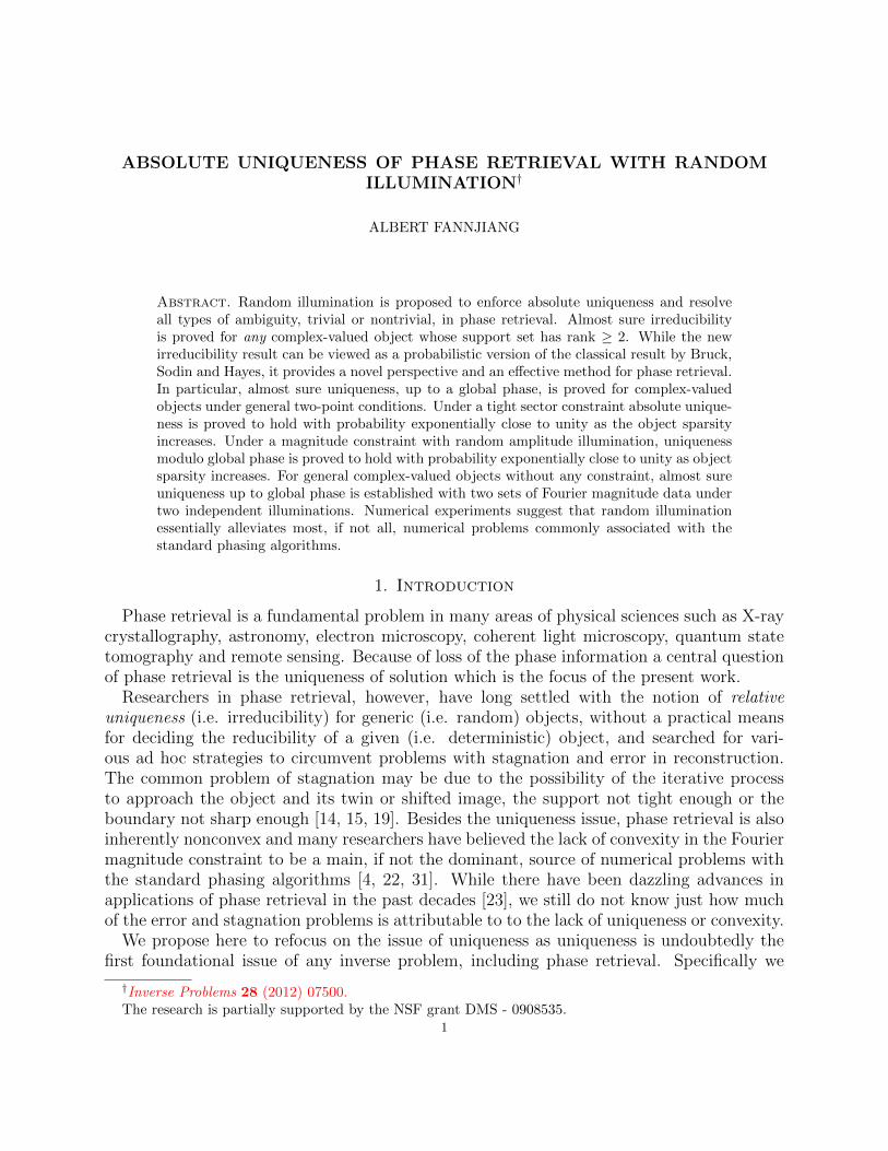
Figure 1. Illumination of a partially transparent object (the blue oval) witha deterministic (a) or random field λ created by a diffuser (b) followed by anintensity measurement of the diffraction pattern. In the case of wave frontreconstruction, the random modulator is placed at the exit pupil instead ofthe entrance pupil as in (b).

will first establish uniqueness in the absolute sense with random illumination under general,physically reasonable constraints (Figure 1) and secondly demonstrate that even thoughthe convexity issue remains unresolved, phasing with random illumination can drasticallyimprove the quality of reconstruction and reduce the numbers of Fourier magnitude dataand numerical iterations.

To fix the idea, consider the discrete version of the phase retrieval problem: Let n =(n1, · · · , nd) ∈ Zd and z = (z1, · · · , zd) ∈ Cd. Define the multi-index notation zn =zn11 zn2

2 · · · zndd . Let f(n) be a finite complex-valued function defined on Zd vanishing out-

side the finite lattice

N =�0 ≤ n ≤ N

�

for N = (N1, · · · , Nd) ∈ Nd. We use the notation m ≤ n for mj ≤ nj, ∀j. The z-transformof a finite sequence f(n) is given by

F (z) =�

n

f(n)z−n.

The Fourier transform can be obtained from the z-transform as

F (w) = F (ei2πw1 , · · · , ei2πwd) =�

n

f(n)e−i2πn·w, w = (w1, · · · , wd) ∈ [0, 1]d

by some abuse of notation. The discrete phase retrieval problem is to determine f(n) fromthe knowledge of the Fourier magnitude |F (w)|, ∀w ∈ [0, 1]d.

The question of uniqueness was partially answered in [4, 14, 15] which says that in dimen-sion two or higher and with the exception of a measure zero set of finite sequences phaseretrieval has a unique solution up to the equivalence class of “trivial associates” (i.e. relativeuniqueness). These trivial, but omnipresent, ambiguities include constant global phase,

f(n) −→ eiθf(n), for some θ ∈ [0, 2π],2

(b)

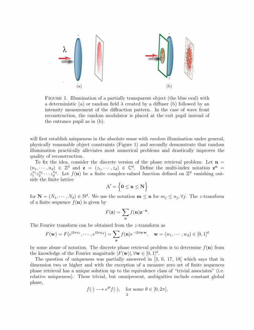
Figure 1. Illumination of a partially transparent object (the blue oval) witha deterministic (a) or random field λ created by a diffuser (b) followed by anintensity measurement of the diffraction pattern. In the case of wave frontreconstruction, the random modulator is placed at the exit pupil instead ofthe entrance pupil as in (b).

will first establish uniqueness in the absolute sense with random illumination under general,physically reasonable object constraints (Figure 1) and secondly demonstrate that randomillumination practically alleviates most numerical problems and drastically improves thequality of reconstruction.

To fix the idea, consider the discrete version of the phase retrieval problem: Let n =(n1, · · · , nd) ∈ Zd and z = (z1, · · · , zd) ∈ Cd. Define the multi-index notation zn =zn1

1 zn22 · · · zndd . Let f(n) be a finite complex-valued function defined on Zd vanishing out-

side the finite lattice

N ={

0 ≤ n ≤ N}

for N = (N1, · · · , Nd) ∈ Nd. We use the notation m ≤ n for mj ≤ nj,∀j. The z-transformof a finite sequence f(n) is given by

F (z) =∑

n

f(n)z−n.

The Fourier transform can be obtained from the z-transform as

F (w) = F (ei2πw1 , · · · , ei2πwd) =∑

n

f(n)e−i2πn·w, w = (w1, · · · , wd) ∈ [0, 1]d

by some abuse of notation. The discrete phase retrieval problem is to determine f(n) fromthe knowledge of the Fourier magnitude |F (w)|, ∀w ∈ [0, 1]d.

The question of uniqueness was partially answered in [3, 6, 17, 18] which says that indimension two or higher and with the exception of a measure zero set of finite sequencesphase retrieval has a unique solution up to the equivalence class of “trivial associates” (i.e.relative uniqueness). These trivial, but omnipresent, ambiguities include constant globalphase,

f(·) −→ eiθf(·), for some θ ∈ [0, 2π],2

spatial shift

f(·) −→ f(·+ m), for some m ∈ Zd,and conjugate inversion

f(·) −→ f ∗(N− ·).Conjugate inversion produces the so-called twin image.

This landmark uniqueness result, however, does not address the following issues. First, agiven object array, there is no way of deciding a priori the irreducibility of the correspondingz-transform and the relative uniqueness of the phasing problem. Secondly, although visuallyno different from the true image the trivial associates (particularly spatial shift and conjugateinversion) nevertheless “confuse” the standard numerical iterative processes and cause seriousstagnation [14, 15, 25, 31].

In this paper, we study the notation of absolute uniqueness: if two finite objects f andg give rise to the same Fourier magnitude data, then f = g unequivocally. More impor-tantly, we present the approach of random (phase or amplitude) illumination to the absoluteuniqueness of phase retrieval. The idea of random illumination is related to coded-apertureimaging whose utility in other imaging contexts than phase retrieval has been establishedexperimentally [1, 2, 5, 8, 29, 32] as well as mathematically [9, 28].

Our basic tool is an improved version (Theorem 2) of the irreducibility result of [17, 18]with, however, a completely different perspective and important practical implications. Themain difference is that while the classical result [17, 18] works with generic (thus random)objects from a certain ensemble Theorem 2 can deal with a given, deterministic object whosesupport has rank ≥ 2. This improvement is achieved by endowing the probability measureon the ensemble of illuminations, which we can manipulate, instead of the space of objects,which we can not control, as in the classical setting.

On the basis of almost sure irreducibility, the mere assumption that the phases or magni-tudes of the object at two arbitrary points lie in a countable set enforces uniqueness, up to aglobal phase, in phase retrieval with a single random illumination (Theorem 3). The absoluteuniqueness can be enforced then by imposing the positivity constraint (Corollary 1). Forobjects satisfying a tight sector condition, absolute uniqueness is valid with high probabilitydepending on the object sparsity for either phase or amplitude illumination (Theorem 4).For complex-valued objects under a magnitude constraint, uniqueness up to a global phaseis valid with high probability (Theorem 5). For general complex-valued objects, almost sureuniqueness, up to global phase, is proved for phasing with two independent illuminations(Theorem 6).

The paper is organized as follows. In Section 2 we discuss various sources of ambiguity.In Section 3 we prove the almost sure irreducibility (Theorem 2 and Appendix). In Section4 we derive the uniqueness results (Theorem 3, 4, 5, 6 and Corollary 1). We demonstratephasing with random illumination in Section 5. We conclude in Section 6.

2. Sources of ambiguity

As commented before the phase retrieval problem does not have a unique solution. Nev-ertheless, the possible solutions are constrained as stated in the following theorem [17, 27].

3

Theorem 1. Let the z-transform F (z) of a finite complex-valued sequence {f(n)} be givenby

F (z) = αz−mp∏

k=1

Fk(z), m ∈ Nd, α ∈ C(1)

where Fk, k = 1, ..., p are nontrivial irreducible polynomials. Let G(z) be the z-transform ofanother finite sequence g(n). Suppose |F (w)| = |G(w)|,∀w ∈ [0, 1]d. Then G(z) must havethe form

G(z) = |α|eiθz−p(∏

k∈IFk(z)

)(∏

k∈IcF ∗k (1/z∗)

), p ∈ Nd, θ ∈ R

where I is a subset of {1, 2, ..., p}.To start, it is convenient to write

|F (w)|2 =N∑

n=−N

∑

m∈Nf(m + n)f ∗(m)e−i2πn·w

=N∑

n=−NCf (n)e−i2πn·w(2)

where

Cf (n) =∑

m∈Nf(m + n)f ∗(m)(3)

is the autocorrelation function of f . Note the symmetry C∗f (n) = Cf (−n).The theorem then follows straightforwardly from the equality between the autocorrelation

functions of f and g, because F (w)F ∗(w) = G(w)G∗(w), and the unique factorization ofpolynomials (see [27] for more details).

Remark 1. If the finite array f(n) is known a priori to vanish outside the lattice N , thenby Shannon’s sampling theorem for band-limited functions the sampling domain for w canbe limited to the finite regular grid

M ={

(k1, · · · , kd) : ∀j = 1, · · · , d & kj = 0,1

2Nj + 1,

2

2Nj + 1, · · · , 2Nj

2Nj + 1.}

(4)

since |F (w)|2 is band-limited to the set −N ≤ n ≤ N.

There are three sources of ambiguity. First, the linear phase term z−m in (1) remainundetermined because the autocorrelation operation destroys information about spatial shift.The unspecified constant phase θ is another source of ambiguity.

To understand the physical meaning of the operation

F (z) −→ z−NF ∗(1/z∗)

consider the case d = 1

z−NF ∗(1/z∗) = f ∗(0)z−N + f ∗(1)z1−N + · · ·+ f ∗(N)4

which is the z-transform of the conjugate space-inversed array {f ∗(N), f ∗(N−1), · · · , f ∗(0)}.The same is true in multi-dimensions.

The subtlest form of ambiguity is caused by partial conjugate inversion on some, but notall, factors of a factorable object, with a reducible z-transform, without which the conjugateinversion, like spatial shift and global phase, is global in nature and considered “trivial” inthe literature (even though the twin image may have an opposite orientation).

In this paper, we consider both types, trivial and nontrivial, of ambiguity, as they bothcan degrade the performance of phasing schemes. Our main purpose is to show by rigorousanalysis that with random illumination it is possible to eliminate all ambiguities at once.

3. Irreducibility

Random illumination amounts to replacing the original object f(n) by

f(n) = f(n)λ(n)(5)

where λ(n), representing the incident field, is a known array of samples of random variables(r.v.s). The idea is to first modify the object by the encoding array λ(n) so that phaseretrieval has unique solution and then use the prior knowledge of λ to recover f .

Nearly independent random illumination can be produced by a diffuser placed near theobject, cf. Figure 1. The illumination field can be randomly modulated in phase only withthe use computer generated holograms [5], random phase plates [1, 29] and liquid crystalphase-only panels [8]. One of the best known amplitude masks is uniformly redundant array[12] and its variants [16]. The advantage of phase mask, compared to amplitude mask, is thelossless energy transmission of an incident wavefront through the mask. By placing eitherphase or amplitude mask at a distance from the object, one can create an illumination fieldmodulated in both amplitude and phase in a way dependent on the distance [32].

Let λ(n) be continuous r.v.s with respect to the Lebesgue measure on S1 (the unit circle),R or C. The case of S1 can be facilitated by a random phase modulator with

λ(n) = eiφ(n)(6)

where φ(n) are continuous r.v.s on [0, 2π] while the case of R can be facilitated by a randomamplitude modulator. The case of C involves simultaneously both phase and amplitudemodulations. More generally, λ(n) can be any continuous r.v. on a zero-containing realalgebraic variety V(n) ⊂ C ' R2. For example R and S1 can be viewed as real projectivevarieties defined by the polynomial equations y = 0 and x2 + y2 − 1 = 0, respectively, onthe complex plane identified as R2. For technical reason, we will focus on the real varietieswhich contain the origin. We call such varieties zero-containing varieties which preclude thecase of S1.

The support Σ of a polynomial F (z) is the set of exponent vectors in Nd with nonzerocoefficients. The rank of the support set is the dimension of its convex hull.

Theorem 2. Let {f(n)} be a finite complex-valued array whose support has rank ≥ 2 andtouches all the coordinate hyperplanes {nj = 0 : j = 1, · · · , d}. Let {λ(n)} be continuous r.v.son zero-containing real algebraic varieties {V(n)} in C(' R2) with an absolutely continuousjoint distribution with respect to the standard product measure on

∏n∈Σ V(n) where Σ ⊂ Nd

5

is the support set of {f(n)}. Then the z-transform of f(n) = f(n)λ(n) is irreducible withprobability one.

Remark 2. If the object support does not touch all the coordinate hyperplanes, then the theirreducibility holds true, up to some monomial of z. In view of Theorem 1 this is sufficientfor our purpose.

Remark 3. The theorem does not hold if the rank-2 condition fails. For example, let p(z)be any monomial and consider

F (z) =∑

j

cjpj(z)(7)

which is reducible for any cj ∈ C, except when F is a monomial, by the fundamental theoremof algebra (of one variable). Another example is the homogeneous polynomials of a sumdegree N

F (z) =∑

i+j=N

cijzi1zj2(8)

which is factorable by, again, the fundamental theorem of algebra.

The proof of Theorem 2 is given in the Appendix.Theorem 2 improves in several aspects on the classical result that the set of the reducible

polynomials has zero measure in the space of multivariate polynomials with real-valuedcoefficients [17, 18]. The main improvement is that while the classical result works withgeneric (thus random) objects Theorem 2 deals with any deterministic object with minimum(and necessary) conditions on its support set. By definition, deterministic objects belongto the measure zero set excluded in the classical setting of [17, 18]. It is both theoreticallyand practically important that Theorem 2 places the probability measure on the ensembleof illuminations, which we can manipulate, instead of the space of objects, which we can notcontrol.

In the next section, we go further to show that with additional, but for all practicalpurposes sufficiently general, constraints on the values of the object, we can essentiallyremove all ambiguities with the only possible exception of global phase factor. This decisivestep distinguishes our method from the standard approach.

4. Uniqueness

Without additional a priori knowledge on the object Theorem 2, however, does not pre-clude the trivial ambiguities such as global phase, spatial shift and conjugate inversion. Forexample, we can produce another finite array {g(n)} that yields the same measurement databy setting

g(n) = eiθf(n + m)λ(n + m)/λ(n)(9)

or

g(n) = eiθf ∗(N− n + m)λ∗(N− n + m)/λ(n)(10)

for θ ∈ [0, 2π] and m ∈ Zd. Expression (9) and (10) are the remaining ambiguities to beaddressed.

6

4.1. Two-point constraint. One important exception is the case of real-valued objectswhen the illumination is complex-valued (the case of S1 or C). In this case, on the one hand(9) produces a complex-valued array with probability one unless m = 0, θ = 0, π and, onthe other hand, (10) is complex-valued with probability one regardless of m. In this case,none of the trivial ambiguities can arise. Indeed, a stronger result is true depending on thenature of random illumination.

Theorem 3. Suppose the object support has rank ≥ 2. Suppose either of the following casesholds:

(i) The phases of the object {f(n)} at two points, where f does not vanish, belong toa known countable subset of [0, 2π] and {λ(n)} are independent continuous r.v.s on zero-containing real algebraic varieties in C such that their angles are continuously distributed on[0, 2π] (e.g. S1 or C)

(ii) The amplitudes of the object {f(n)} at two points, where f does not vanish, be-long to a known measure zero subset of R and {λ(n)} are independent continuous r.v.s onzero-containing real algebraic varieties in C such that their magnitudes are continuously dis-tributed on (0,∞) (e.g. R or C).

Then f is determined uniquely, up to a global phase, by the Fourier magnitude measure-ment on the lattice M with probability one.

Remark 4. For the two-point constraint in case (i) to be convex, it is necessary for theconstraint set to be a singleton, namely the phases of the object at two nonzero points musttake on a single known value. On the other hand, the amplitude constraint in case (ii) cannever be convex unless the set is a singleton and the object phases are the same at the twopoints.

Proof. By Theorem 2 the z-transform of {λ(n)f(n)} is irreducible with probability one. Weprove the theorem case by case.

Case (i): Suppose the phases of f(n1) and f(n2) belong to the coutable set Θ ⊂ [0, 2π]. Letus show the probability that the phase of g(n) as given by (9) with m 6= 0 takes on a valuein Θ at two distinct points is zero.

Since λ(n+m),m 6= 0, and the phases of λ(n) are independent, continuous r.v.s on [0, 2π],the phase of g(n),∀n, is continuously distributed on [0, 2π] for all θ.

Now suppose the phase of g(n0) for some n0 lies in the set Θ. This implies that θ mustbelong to the countable set Θ′ which is Θ shifted by the negative phase of f(n0 + m)λ(n0 +m)/λ(n0). The phase of g(n) at a different location n 6= n0, however, almost surely does nottake on any value in the set Θ for any fixed θ ∈ Θ′ unless m = 0. Since a countable unionof measure-zero sets has zero measure, the probability that the phases of g at two points liein Θ is zero if m 6= 0.

Likewise, λ∗(N− n + m)/λ(n),∀m, has a random phase that is continuously distributedon [0, 2π] and by the same argument the probability that the phases of g as given by (10)at two points lie in Θ is zero.

7

Case (ii): Suppose the amplitudes of f(n1) and f(n2) belong to the measure zero set A.Since λ(n + m),m 6= 0, and λ(n) are independent and continuously distributed on R orC, the amplitude of g(n) as given by (9) is continuously distributed on R and hence theprobability that the amplitude of g(n) as given by (9) belongs to A at any n is zero.

Now consider g(n) given by (10). Suppose that the amplitude of g(n0) belongs to A atsome n0. This is possible only for n0 = (N + m)/2 in which case g(n0) = eiθf ∗(n0). Theamplitude of g(n),n 6= n0, has a continuous distribution on R and zero probability to lie inA.

The global phase θ, however, can not be determined uniquely in either case.�

The global phase factor can be determined uniquely by additional constraint on the valuesof the object. For example, the following result follows immediately from Theorem 3 (i).

Corollary 1. Suppose that {f(n)} is real and nonnegative and its support has rank ≥ 2.Suppose that {λ(n)} are independent continuous r.v.s on zero-containing real algebraic vari-eties in C such that their phases are continuously distributed on [0, 2π] (e.g. S1 or C). Then{f(n)} can be determined absolutely uniquely with probability one.

Proof. With a real, positive object, the countable set for phase is the singleton {0} and theglobal phase is uniquely fixed. �

4.2. Sector constraint. More generally, we consider the sector constraint that the phasesof {f(n)} belong to [a, b] ⊂ [0, 2π]. For example, the class of complex-valued objects relevantto X-ray diffraction typically have nonnegative real and imaginary parts where the real partis the effective number of electrons coherently diffracting photons, and the imaginary partrepresents the attenuation [25]. For such objects, [a, b] = [0, π/2].

Generalizing the argument for Theorem 3 we can prove the following.

Theorem 4. Suppose the object support has rank ≥ 2. Let the finite object {f(n)} satisfythe sector constraint that the phases of {f(n)} belong to [a, b] ⊂ [0, 2π]. Let S be the sparsity(the number of nonzero elements) of the object.

(i) Suppose {λ(n)} are independent, identically distributed (i.i.d.) continuous r.v.s onzero-containing real algebraic varieties in C such that their phases {φ(n)} are uniformly dis-tributed on [0, 2π] (e.g. the random phase illumination (6)). Then with probability at least1− |N ||b− a|[S/2](2π)−[S/2] the object f is uniquely determined, up to a global phase, by theFourier magnitude measurement. Here [S/2] is the greatest integer at most S/2.

(ii) Consider the random amplitude illumination with i.i.d. continuous r.v.s {λ(n)} ⊂ Rthat are equally likely negative or positive, i.e. P{λ(n) > 0} = P{λ(n) < 0} = 1/2,∀n.Suppose |b− a| ≤ π. Then with probability at least 1− |N |2−[(S−1)/2] the object f is uniquelydetermined, up to a global phase, by the Fourier magnitude measurement.

In both cases, the global phase is uniquely determined if the sector [a, b] is tight in the sensethat no proper interval of [a, b] contains all the phases of the object.

Proof. Case (i): Consider first the expression (9) with any m 6= 0 and the [S/2] independentlydistributed r.v.s of g(n) corresponding to [S/2] nonoverlapping pairs of points {n,n + m}.

8

The probability for every such the phase of g(n) to lie in the sector [a, b] is |b− a|/(2π) forany θ and hence the probability for all g(n) with m 6= 0, θ 6= 0, to lie in the sector is atmost |b − a|[S/2](2π)−[S/2]. The union over m 6= 0 of these events has probability at most|N ||b− a|[S/2](2π)−[S/2].

Likewise the probability for all g(n) given by (10) to lie in the first quadrant for any m isat most |N ||b− a|[S/2](2π)−[S/2].

Case (ii): For (9) with any m 6= 0 the [S/2] independently distributed random variablesg(n) corresponding to [S/2] nonoverlapping pairs of points {n,n + m}, satisfy the sectorconstraint with probability at most 2−[S/2] if |b− a| ≤ π. Hence the probability that all g(n)with m 6= 0 satisfy the sector constraint is at most |N |2−[S/2].

For (10) with θ = 0 and any m, g(n0) = f(n0) at n0 = (N + m)/2 and hence g(n0) liesin the first quadrant with probability one. For n 6= n0, g(n) satisfies the sector constraintwith probability 1/2 if |b − a| ≤ π. Now the [(S − 1)/2] independently distributed r.v.sg(n) corresponding to nonoverlapping pairs of points {n,n + m},n 6= n0, satisfy the sectorconstraint with probability at most 2−[(S−1)/2] if |b− a| ≤ π. Hence the probability that allg(n) given by (10) with arbitrary m satisfy the sector constraint is at most |N |2−[(S−1)/2]. �

4.3. Magnitude constraint. Likewise if the object satisfies a magnitude constraint thenwe can use random amplitude illumination to enforce uniqueness (up to a global phase).

Theorem 5. Suppose that the object support has rank ≥ 2. Suppose that K pixels of thecomplex-valued object f satisfy the magnitude constraint 0 < a ≤ |f(n)| ≤ b and that{λ(n)} are i.i.d. continuous r.v.s on zero-containing real algebraic varieties in C withP{|λ(n)/λ(n′)| > b/a or |λ(n)/λ(n′)| < a/b} = 1 − p > 0 for n 6= n′. Then the objectf is determined uniquely, up to a global phase, by the Fourier magnitude data on M, withprobability at least 1− |N |p[(K−1)/2].

Proof. The proof is similar to that for Theorem 4(ii).For (9) with any m 6= 0 the [K/2] independently distributed random variables g(n) corre-

sponding to [K/2] nonoverlapping pairs of points {n,n + m} satisfy 0 < a ≤ |g(n)| ≤ b withprobability less than p−[K/2] for any θ. Hence the probability that g(n) with m 6= 0 satisfythe magnitude constraint at K or more points is at most |N |p−[K/2].

For (10) with any m, |g(n0)| = |f(n0)| at n0 = (N + m)/2 and hence g(n0) satisfies themagnitude constraint with probability one. For n 6= n0, there is at most probability p forg(n) to satisfy the magnitude constraint. By independence, the [(K − 1)/2] independentlydistributed r.v.s g(n) corresponding to nonoverlapping pairs of points {n,n + m},n 6= n0,satisfy the magnitude constraint with probability at most p[(K−1)/2]. Hence the probabilitythat g(n) given by (10) with arbitrary m satisfy the magnitude constraint at K or morepoints is at most |N |p[(K−1)/2].

The global phase factor is clearly undetermined. �

As in Theorem 3 case (ii) the magnitude constraint here, however, is not convex.

4.4. Complex objects without constraint. For general complex-valued objects withoutany constraint, we consider two sets of Fourier magnitude data produced with two indepen-dent random illuminations and obtain almost sure uniqueness modulo global phase.

9

Theorem 6. Let {f(n)} be a finite complex-valued array whose support has rank ≥ 2.Let {λ1(n)} and {λ2(n)} be two independent arrays of r.v.s satisfying the assumptions inTheorem 2.

Then with probability one f(n) is uniquely determined, up to a global phase, by the Fouriermagnitude measurements on M with two illuminations λ1 and λ2.

If the second illumination λ2 is deterministic and results in an irreducible z-transformwhile λ1 is random as above, then the same conclusion holds.

Proof. Let g(n) be another array that vanishes outside N and produces the same data. ByTheorem 1, 2 and Remark 1

g(n) =

{eiθif(n + mi)λi(n + mi)/λi(n)

eiθif ∗(N− n + mi)λ∗i (N− n + mi)/λi(n),

(11)

for some mi ∈ Zd, θi ∈ R, i = 1, 2.Four scenarios of ambiguity exist but because of the independence of λ1(n), λ2(n) none

can arise.First of all, if

g(n) = eiθif(n + mi)λi(n + mi)/λi(n), i = 1, 2

theneiθ1f(n + m1)λ1(n + m1)/λ1(n) = eiθ2f(n + m2)λ2(n + m2)/λ2(n).

This almost surely can not occur unless m1 = m2 = 0, θ1 = θ2 in which case g equals f upto a global phase factor.

The other possibilities can be similarly ruled out:

g(n) = eiθ1f(n + m1)λ1(n + m1)/λ1(n)

= eiθ2f ∗(N− n + m2)λ∗2(N− n + m2)/λ2(n)

and

g(n) = eiθif ∗(N− n + mi)λ∗i (N− n + mi)/λi(n), i = 1, 2(12)

for any mi, θi, i = 1, 2.The same argument above applies to the case of deterministic λ2 if the resulting z-

transform is irreducible.�

5. Numerical examples

Our previous numerical study [10] and the following numerical examples give a glimpse ofhow the quality and efficiency of reconstruction can be improved by random illumination.

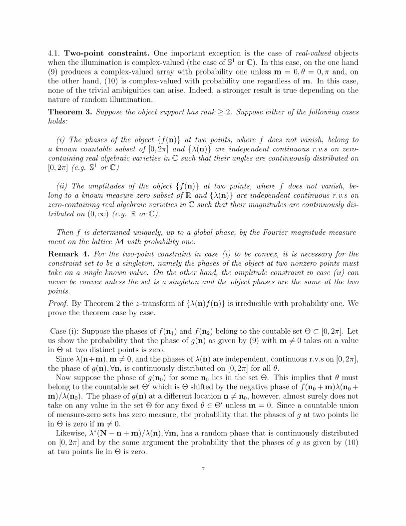
We test the case of random phase illumination on a real, positive 269× 269 image consist-ing of the original 256× 256 Cameraman in the middle, surrounded by a black margin (zeropadding) of 13 pixels in width (Figure 2(a)). We synthesize and sample the Fourier magni-tudes at the Nyquist rate (Remark 1) and implement the standard Error Reduction (ER)

10

(a)

150 ER(SR = 4)

||fk fk+1||/||fk|| = 1.9293e 08% projerr = 5.7341e 08% residual = 5.0849e 08%(b)

20 40 60 80 100 120 1400

0.05

0.1

0.15

0.2

0.25

0.3

0.35

0.4

0.45

0.5

||fk − f

k+1|| / ||f

k|| at each iteration

iteration

||f k

− f

k+

1|| / ||f

k||

(c)

20 40 60 80 100 120 1400

0.05

0.1

0.15

0.2

0.25

0.3

0.35

0.4

0.45

0.5

relative residual at each iteration

iteration

rela

tive r

esid

ual

(d)

Figure 2. ER reconstruction with random phase illumination: (a) recoveredimage (b) difference between the true and recovered images (c) relative change

‖fk+1 − fk‖/‖fk‖ (e) relative residual ‖|F | − |ΦΛfk|‖/‖F‖ versus number ofiterations.

and Hybrid-Input-Output (HIO) algorithms in the framework of the oversampling method[24, 25]. By Corollary 1, absolute uniqueness holds with a random phase illumination.

Let Φ and Λ be the Fourier transform and the diagonal matrix diag[λ(n)] representingthe illumination. For the uniform illumination Λ = I. The ER and HIO algorithms aredescribed below.

ER algorithm

Input: Fourier magnitude data {F (w)}, initial guess f0.Iterations:• Update Fourier phase: Gk = ΦΛfk = |Gk(w)|eiθk(w).

• Update Fourier magnitude: G′k(w) = |F (w)|eiθk(w).

• Impose object constraint fk+1(n) =

{f ′k(n) if f ′k(n) = Λ−1Φ∗G′k(n) ≥ 00 otherwise

11

(a)

100 HIO + 50 ER(SR = 4)

||fk fk+1||/||fk|| = 4.651e 07% projerr = 1.3302e 06% residual = 1.1676e 06%(b)

20 40 60 80 100 120 1400

0.05

0.1

0.15

0.2

0.25

0.3

0.35

0.4

0.45

0.5

||fk − f

k+1|| / ||f


iteration

||f k

− f

k+

1|| / ||f

k||

(c)

20 40 60 80 100 120 1400

0.05

0.1

0.15

0.2

0.25

0.3

0.35

0.4

0.45

0.5


iteration

rela

tive r

esid

ual

(d)

Figure 3. HIO reconstruction with random phase illumination: (a) recoveredimage (b) difference between the true and recovered images (c) relative change(e) relative residual versus number of iterations. The final 50 iterations areER.

20 40 60 80 100 120 1400

0.1

0.2

0.3

0.4

0.5

0.6

0.7

0.8

0.9

1relative error at each iteration

iteration

rela

tive e

rror

of th

e im

age

(a)

20 40 60 80 100 120 1400

0.1

0.2

0.3

0.4

0.5

0.6

0.7

0.8

0.9


iteration

rela

tive e

rror

of th

e im

age

(b)

Figure 4. Relative error ‖fk − f‖/‖f‖ with (a) ER and (b) HIO versusnumber of iterations.

12

(a)

1050 ER(SR = 8)

||X Xrectwin||/||X|| = 72.809% projerr = 4.4077% residual = 4.4075%(b)

100 200 300 400 500 600 700 800 900 10000

0.05

0.1

0.15

0.2

0.25

0.3

0.35

0.4

0.45

0.5

||fk − f

k+1|| / ||f


iteration

||f k

− f

k+

1|| / ||f

k||

(c)

100 200 300 400 500 600 700 800 900 10000

0.05

0.1

0.15

0.2

0.25

0.3

0.35

0.4

0.45

0.5


iteration

rela

tive r

esid

ual

(d)

Figure 5. ER reconstruction with uniform illumination: (a) recovered image(b) difference between the true and recovered images (c) relative change (d)relative residual versus number of iterations.

In the original version of HIO [13], the hard thresholding is replaced by

fk+1(n) =

{f ′k(n) if f ′k(n) = Λ−1Φ∗G′k(n) ≥ 0

fk(n)− βf ′k(n) otherwise

where the feedback parameter β = 0.9 is used in the simulations. ER has the desirable

property that the residual ‖|F | − |Gk|‖ is reduced after each iteration under either uniformor random phase illumination [13, 11]. When absolute uniqueness holds, a vanishing residualthen implies a vanishing reconstruction error.

Figure 2 shows the results of ER reconstruction with random phase illumination. The ERiteration converges to the true image after 40 iterations. For HIO reconstruciton we apply50 ER iterations after 100 HIO iterations as suggested in [22]. HIO has essentially the sameperformance as ER (Figure 3 (a), (b)). The relative residual curve, Figure 3(d), and therelative error curve, Figure 4, however, indicate a small improvement by HIO. The closeproximity between the vanishing residual curve and the vanishing error curve for ER andHIO reflects the absolute uniqueness under random illumination.

13

(a)

1000 HIO + 50 ER(SR = 4)

||fk fk+1||/||fk|| = 0.033041% projerr = 1.1033% residual = 1.1023%(b)

100 200 300 400 500 600 700 800 900 10000

0.05

0.1

0.15

0.2

0.25

0.3

0.35

0.4

0.45

0.5

||fk − f

k+1|| / ||f


iteration

||f k

− f

k+

1|| / ||f

k||

(c)

100 200 300 400 500 600 700 800 900 10000

0.05

0.1

0.15

0.2

0.25

0.3

0.35

0.4

0.45

0.5


iteration

rela

tive r

esid

ual

(d)

Figure 6. HIO reconstruction: (a) recovered image (b) difference betweenthe true and recovered images (c) relative change (d) relative residual versusnumber of iterations. The final 50 iterations are ER, causing a dip in therelative change and residual.

100 200 300 400 500 600 700 800 900 10000

0.1

0.2

0.3

0.4

0.5

0.6

0.7

0.8

0.9


iteration

rela

tive e

rror

of th

e im

age

(a)

100 200 300 400 500 600 700 800 900 10000

0.1

0.2

0.3

0.4

0.5

0.6

0.7

0.8

0.9


iteration

rela

tive e

rror

of th

e im

age

(b)

Figure 7. Relative error with (a) ER and (b) HIO versus number of iterations.

14

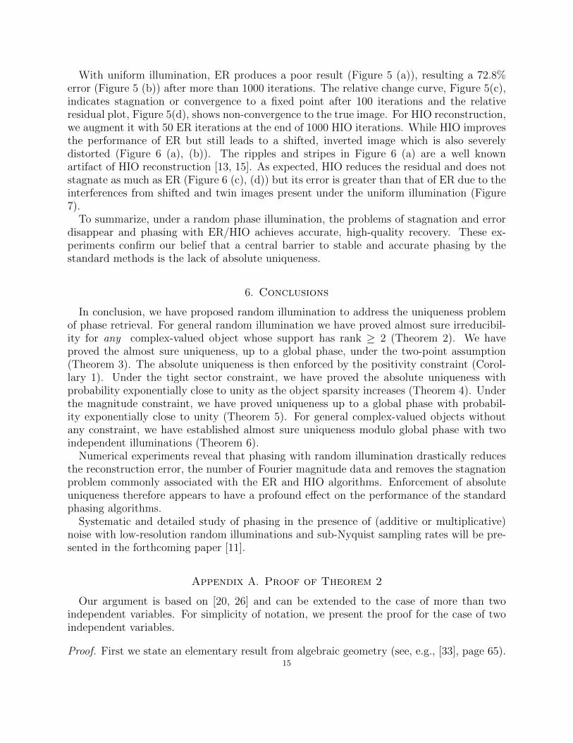
With uniform illumination, ER produces a poor result (Figure 5 (a)), resulting a 72.8%error (Figure 5 (b)) after more than 1000 iterations. The relative change curve, Figure 5(c),indicates stagnation or convergence to a fixed point after 100 iterations and the relativeresidual plot, Figure 5(d), shows non-convergence to the true image. For HIO reconstruction,we augment it with 50 ER iterations at the end of 1000 HIO iterations. While HIO improvesthe performance of ER but still leads to a shifted, inverted image which is also severelydistorted (Figure 6 (a), (b)). The ripples and stripes in Figure 6 (a) are a well knownartifact of HIO reconstruction [13, 15]. As expected, HIO reduces the residual and does notstagnate as much as ER (Figure 6 (c), (d)) but its error is greater than that of ER due to theinterferences from shifted and twin images present under the uniform illumination (Figure7).

To summarize, under a random phase illumination, the problems of stagnation and errordisappear and phasing with ER/HIO achieves accurate, high-quality recovery. These ex-periments confirm our belief that a central barrier to stable and accurate phasing by thestandard methods is the lack of absolute uniqueness.

6. Conclusions

In conclusion, we have proposed random illumination to address the uniqueness problemof phase retrieval. For general random illumination we have proved almost sure irreducibil-ity for any complex-valued object whose support has rank ≥ 2 (Theorem 2). We haveproved the almost sure uniqueness, up to a global phase, under the two-point assumption(Theorem 3). The absolute uniqueness is then enforced by the positivity constraint (Corol-lary 1). Under the tight sector constraint, we have proved the absolute uniqueness withprobability exponentially close to unity as the object sparsity increases (Theorem 4). Underthe magnitude constraint, we have proved uniqueness up to a global phase with probabil-ity exponentially close to unity (Theorem 5). For general complex-valued objects withoutany constraint, we have established almost sure uniqueness modulo global phase with twoindependent illuminations (Theorem 6).

Numerical experiments reveal that phasing with random illumination drastically reducesthe reconstruction error, the number of Fourier magnitude data and removes the stagnationproblem commonly associated with the ER and HIO algorithms. Enforcement of absoluteuniqueness therefore appears to have a profound effect on the performance of the standardphasing algorithms.

Systematic and detailed study of phasing in the presence of (additive or multiplicative)noise with low-resolution random illuminations and sub-Nyquist sampling rates will be pre-sented in the forthcoming paper [11].

Appendix A. Proof of Theorem 2

Our argument is based on [20, 26] and can be extended to the case of more than twoindependent variables. For simplicity of notation, we present the proof for the case of twoindependent variables.

Proof. First we state an elementary result from algebraic geometry (see, e.g., [33], page 65).15

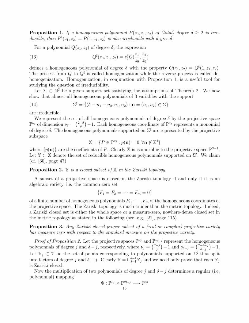
Proposition 1. If a homogeneous polynomial P (z0, z1, z2) of (total) degree δ ≥ 2 is irre-ducible, then P [(z1, z2) ≡ P (1, z1, z2) is also irreducible with degree δ.

For a polynomial Q(z1, z2) of degree δ, the expression

Q](z0, z1, z2) = zδ0Q(z1

z0

,z2

z0

)(13)

defines a homogeneous polynomial of degree δ with the property Q(z1, z2) = Q](1, z1, z2).The process from Q to Q] is called homogenization while the reverse process is called de-homogenization. Homogenization, in conjunction with Proposition 1, is a useful tool forstudying the question of irreducibility.

Let Σ ⊂ N2 be a given support set satisfying the assumptions of Theorem 2. We nowshow that almost all homogeneous polynomials of 3 variables with the support

Σ] = {(δ − n1 − n2, n1, n2) : n = (n1, n2) ∈ Σ}(14)

are irreducible.We represent the set of all homogeneous polynomials of degree δ by the projective space

Pνδ of dimension νδ =(

2+δδ

)−1. Each homogeneous coordinate of Pνδ represents a monomial

of degree δ. The homogeneous polynomials supported on Σ] are represented by the projectivesubspace

X = {P ∈ Pνδ : p(n) = 0,∀n 6∈ Σ]}where {p(n)} are the coefficients of P . Clearly X is isomorphic to the projective space PS−1.Let Y ⊂ X denote the set of reducible homogeneous polynomials supported on Σ]. We claim(cf. [30], page 47)

Proposition 2. Y is a closed subset of X in the Zariski topology.

A subset of a projective space is closed in the Zariski topology if and only if it is analgebraic variety, i.e. the common zero set

{F1 = F2 = · · · = Fm = 0}of a finite number of homogeneous polynomials F1, · · · , Fm of the homogeneous coordinates ofthe projective space. The Zariski topology is much cruder than the metric topology. Indeed,a Zariski closed set is either the whole space or a measure-zero, nowhere-dense closed set inthe metric topology as stated in the following (see, e.g. [21], page 115).

Proposition 3. Any Zariski closed proper subset of a (real or complex) projective varietyhas measure zero with respect to the standard measure on the projective variety.

Proof of Proposition 2. Let the projective spaces Pνj and Pνδ−j represent the homogeneouspolynomials of degree j and δ− j, respectively, where νj =

(2+jj

)−1 and νδ−j =

(2+δ−jδ−j

)−1.

Let Yj ⊂ Y be the set of points corresponding to polynomials supported on Σ] that splitinto factors of degree j and δ− j. Clearly Y = ∪δ−1

j=1Yj and we need only prove that each Yj

is Zariski closed.Now the multiplication of two polynomials of degree j and δ− j determines a regular (i.e.

polynomial) mapping

Φ : Pνj × Pνδ−j −→ Pνδ16

in the following way. Let G(z) and H(z) be homogeneous polynomials of degrees j and δ−j,respectively. Let {g(n)} and {h(n)} be the coefficients of G and H, respectively. Then thecoefficients of the image point Φ(G,H) are given by

{ ∑

|n|=δ−jg(m− n)h(n) : |m| = m0 +m1 +m2 = δ

}.(15)

In other words Φ is bilinear in {g(n)} and {h(n)} and thus is regular. Clearly we have

Yj = Φ(Pνj × Pνδ−j

)∩ X.

Since the product of projective spaces is a projective variety and the image of a projectivevariety under a regular mapping is Zariski closed [30], Yj is a Zariski closed subset of X.

�

Let Σ = {n1,n2, · · · ,nS} and let the ensemble of polynomials corresponding to {λ(n)f(n)}be identified with∏

n∈Σ

f(n)V(n) = (f(n1)V(n1))× (f(n2)V(n2))× · · · × (f(nS)V(nS))

wherefV = {(xf1 − yf2, xf2 + yf1) ∈ R2 : f1 = <(f), f2 = =(f), (x, y) ∈ V}.

Note that fV is a zero-containing real algebraic variety in R2 if V is also. Modulo somemonomial,

∏n∈Σ f(n)V(n) can be identified with a real sub-variety of RP2S−1 which can be

mapped into the complex projective space PS−1 via the projection:

P : RP2S−1 −→ PS−1

by enlarging the equivalence classes. Let

V = P(∏

n∈Σ

f(n)V(n))⊂ X.

Clearly Y ∩ V is a zero-containing real algebraic subvariety in V. To show Y ∩ V is ameasure-zero subset of V we only need to show that Y∩V ( V in view of Proposition 2 and3.

Following the suggestion in [20], we now prove

Proposition 4. Y ∩ V ( V.

Proof of Proposition 4. It suffices to find one irreducible polynomial in V.The argument is based on two observations. First the polynomial

F (x, y, z) = axr + byr + czr(16)

is irreducible for any positive integer r and any nonzero coefficients a, b, c. This follows fromthe fact that the criticality equations Fx = Fy = Fz = 0 have no solution in P2 and thus thealgebraic variety F = 0 is non-singular and not a union of isolated points.

Secondly, for any Σ satisfying the assumptions of Theorem 2, there exists a set T ⊂ Σ] ofthree points which can be transformed into {(r, 0, 0), (0, r, 0), (0, 0, r)}, the support of (16),under a rational map.

We separate the analysis of the second observation into two cases.17

Case 1: (0, 0) ∈ Σ. Then there are at least two other points, say (m,n), (p, q), belongingto Σ. Without loss of generality, we assume p+ q = δ. Because Σ has rank 2, mq − np 6= 0.

We look for the rational mapping

z1 = xk11yk21zk31 , z2 = xk12yk22zk32 , z0 = xk13yk23zk33(17)

with kij ∈ Z that maps the polynomial

P (z0, z1, z2) = czδ0 + azδ−m−n0 zm1 zn2 + bzp1z

q2

to F (x, y, z). This amounts to a linear transformation from the set of independent vectors

(m,n, δ −m− n), (p, q, 0), (0, 0, δ)

to the set {(r, 0, 0), (0, r, 0), (0, 0, r)}. This transformation can be accomplished by the fol-lowing matrix

r

m p 0n q 0

δ −m− n 0 δ

−1

=r

δ(mq − np)

qδ −nδ −q(δ −m− n)−pδ mδ p(δ −m− n)

0 0 mq − np

(18)

where the divisor is nonzero. To ensure integer entries in (18) we set

r = δ(mq − np)and obtain the transformation matrix

k11 k12 k13

k21 k22 k23

k31 k32 k33

=

qδ −nδ −q(δ −m− n)−pδ mδ p(δ −m− n)

0 0 mq − np

Case 2: (m, 0), (0, n) ∈ Σ for some positive integers m,n. Then there is at least anotherpoint (p, q) ∈ Σ such that (m, 0), (0, n), (p, q) are not collinear, which means mn−np−mq 6=0.

Suppose p+ q = δ. Consider the polynomial

P (z0, z1, z2) = azδ−m0 zm1 + bzδ−n0 zn2 + czp1zq2.

By the same analysis above the form (16) can be achieved by the transformation matrix

r

m 0 p0 n q

δ −m δ − n 0

−1

=r

δ(mn−mq − np)

−q(δ − n) q(δ −m) −n(δ −m)p(δ − n) −p(δ −m) −m(δ − n)−pn −mq mn

which has integer entries if r is a multiple of δ(mn−mq − np). With the choice

r = δ(mn−mq − np)the transformation matrix becomes

k11 k12 k13

k21 k22 k23

k31 k32 k33

=

−q(δ − n) q(δ −m) −n(δ −m)p(δ − n) −p(δ −m) −m(δ − n)−pn −mq mn

.

Suppose n = δ. Consider the polynomial

P (z0, z1, z2) = azn−m0 zm1 + bzn2 + czn−p−q0 zp1zq2.

18

The form (16) can be achieved by the transformation matrix

r

m 0 p0 n q

n−m 0 n− p− q

−1

=r

n(mn−mq − np)

n(n− p− q) q(n−m) n(m− n)

0 mn−mq − np 0−pn −mq mn

.

With

r = n(mn−mq − np)the transformation matrix becomes

k11 k12 k13

k21 k22 k23

k31 k32 k33

=

n(n− p− q) q(n−m) n(m− n)

0 mn−mq − np 0−pn −mq mn

.

Suppose m = δ. Consider the polynomial

P (z0, z1, z2) = azm1 + bzm−n0 zn2 + czm−p−q0 zp1zq2.

The form (16) can be achieved by the transformation matrix

r

m 0 p0 n q0 m− n m− p− q

−1

=r

m(mn−mq − np)

mn−mq − np 0 0p(m− n) m(m− p− q) m(n−m)−pn −mq mn

.

With

r = m(mn−mq − np)the transformation matrix becomes

k11 k12 k13

k21 k22 k23

k31 k32 k33

=

mn−mq − np 0 0p(m− n) m(m− p− q) m(m− n)−pn −mq mn

.

To conclude the proof of Proposition 4, in any above case, if the polynomial P (z0, z1, z2)is reducible (i.e. has a non-monomial factor), then we can write P = P1P2 and

F (x, y, z) = P1(z0(x, y, z), z1(x, y, z), z2(x, y, z))P2(z0(x, y, z), z1(x, y, z), z2(x, y, z))(19)

where P1, P2 are non-monomial factors. Let l be the lowest (possibly negative) power inx, y, z of Pi(z0(x, y, z), z1(x, y, z), z2(x, y, z)), i = 1, 2. If l ≥ 0, then the factorization (19)implies that F (x, y, z) has a non-monomial factor. If l < 0, then the factorization (19)implies that (xyz)−lF (x, y, z) has a non-monomial factor. Either case contradicts the factthat F is irreducible. So P is irreducible. The proof of Proposition 4 is complete.

�

Continuing the proof of Theorem 2, we have from Propositions 3 and 4 that Y ∩ V is ameasure-zero subset of V. By dehomogenization and Proposition 1 reducible polynomials ofa fixed support Σ under the assumptions of Theorem 2 comprise a measure-zero subset ofall polynomials of the same support. The proof of Theorem 2 is now complete.

�19

Acknowledgements. I am grateful to my colleagues Greg Kuperberg and Brian Osser-man for inspiring discussions on the proof of Theorem 2, an improvement of the earlier versionwhich assumes convexity of the support. I thank my student Wenjing Liao for performingsimulations and producing the figures.

References

[1] P. F. Almoro and S. G. Hanson, “ Random phase plate for wavefront sensing via phase retrieval and avolume speckle field,” Appl. Opt. 47 2979-2987 (2008).

[2] P. F. Almoro, G. Pedrini, P. N. Gundu, W. Osten, S. G. Hanson, “Enhanced wavefront reconstructionby random phase modulation with a phase diffuser,” Opt. Laser Eng. 49 252-257 (2011).

[3] R.H.T. Bates, “Fourier phase problems are uniquely soluble in more than one dimension. I: underlyingtheory,” Optik (Stuttgart) 61, 247-262 (1982).

[4] H.H. Bauschke, P.L. Combettes, and D.R. Luke, “Phase retrieval, error reduction algorithm, and Fienupvariants: a view from convex optimization,” J. Opt. Soc. Am. A 19(7), 1334 - 1345 (2002).

[5] R. Brauer, U. Wojak, F. Wyrowski, O. Bryngdahl, “ Digital diffusers for optical holography,” Opt. Lett.16, 14279 (1991).

[6] Yu. M. Bruck and L. G. Sodin, ”On the ambiguity of the image reconstruction problem,” Opt. Com-mun.30, 304-308 (1979).

[7] E. J. Candes, Y. Eldar, T. Strohmer and V. Voroninski, “ Phase retrieval via matrix completion,”preprint, August 2011.

[8] C. Falldorf, M. Agour, C. v. Kopylow and R. B. Bergmann, “Phase retrieval by means of a spatial lightmodulator in the Fourier domain of an imaging system,” Appl. Opt. 49, 1826-1830 (2010).

[9] A. Fannjiang, “ Exact localization and superresolution with noisy data and random illumination,”Inverse Problems 27 065012 (2011)

[10] A. Fannjiang and W. Liao, “Compressed sensing phase retrieval,” Proceedings of IEEE Asilomar Con-ference on Signals, Systems and Computers, Pacific Grove, CA, Nov 6-9, 2011, pp. 735-738.

[11] A. Fannjiang and W. Liao, “Phase retrieval with random phase illumination,” J. Opt. Soc. Am. A.2012, in press.

[12] E.E. Fenimore, “Coded aperture imaging: the modulation transfer function for uniformly redundantarrays,” Appl. Opt. 19 2465-2471 (1980).

[13] J.R. Fienup, “Phase retrieval algorithms: a comparison, ” Appl. Opt. 21 2758-2769 (1982).[14] J.R. Fienup, “Reconstruction of a complex-valued object from the modulus of its Fourier transform

using a support constraint,” J. Opt. Soc. Am. A 4, 118 -123 (1987).[15] J.R. Fienup and C.C. Wackerman, “Phase-retrieval stagnation problems and solutions,” J. Opt. Soc.

Am. A 3 1897-1907 (1986).[16] S. R. Gottesman and E. E. Fenimore, “New family of binary arrays for coded aperture imaging,” Appl.

Opt. 28, 4344-4352 (1989).[17] M. Hayes, ”The reconstruction of a multidimensional sequence from the phase or magnitude of its

Fourier transform,” IEEE Trans. Acoust. Speech Sign. Proc. 30 140- 154 (1982).[18] M.H. Hayes and J.H. McClellan. “Reducible Polynomials in More Than One Variable.” Proc. IEEE

70(2):197 198, (1982).[19] H. He, “Simple constraint for phase retrieval with high efficiency,” J. Opt. Soc. Am. A23 550 - 556

(2006).[20] G. Kuperberg, personal communication, 2012.[21] J.M. Landsberg, Tensors: Geometry and Applications. American Mathematical Society, Providence,

2012.[22] S. Marchesini, “ A unified evaluation of iterative projection algorithms for phase retrieval,” Rev. Sci.

Instr. 78, 011301 (2007).20

[23] J. Miao, T. Ishikawa, Q. Shen, and T. Earnest, “Extending X-Ray crystallography to allow the imagingof non- crystalline materials, cells and single protein complexes,” Annu. Rev. Phys. Chem. 59, pp.387410 (2008).

[24] J. Miao and D. Sayre, “On possible extensions of X-ray crystallography through diffraction-patternoversampling,” Acta Cryst. A 56 596-605 (2000).

[25] J. Miao, D. Sayre and H.N. Chapman, “Phase retrieval from the magnitude of the Fourier transformsof nonperiodic objects,” J. Opt. Soc. Am. A 15 1662-1669 (1998).

[26] B. Osserman, personal communication, 2012.[27] T.A. Pitts and J. F. Greenleaf, “Fresnel transform phase retrieval from magnitude,” IEEE Trans.

Ultrasonics, Ferroelec. Freq. Contr. 50 (8) 1035-1045 (2003).[28] J. Romberg, “Compressive sensing by random convolution,” SIAM J. Imag. Sci. 2 1098-1128 (2009).[29] J.E. Rothenberg, “ Improved beam smoothing with SSD using generalized phase modulation,” Proc.

SPIE 3047, 713 (1997).[30] I. R. Shafarevich, Basic Algebraic Geometry, Springer-Verlag, Berlin, 1977.[31] H. Stark, Image Recovery: Theory and Applications. New York: Academic Press, 1987.[32] D. Sylman, V. Mico, J. Garcia, and Z. Zalevsky, “Random angular coding for superresolved imaging,”

Appl. Opt. 49 4874-4882 (2010)[33] K. Ueno, Introduction to Algebraic Geometry. American Mathematical Society, Providence, Rhode Is-

land, 1997.

Department of Mathematics, UC Davis, CA 95616-8633. [email protected]

21

Documents

ABSOLUTE UNIQUENESS OF PHASE …fannjiang/home/papers/...ABSOLUTE UNIQUENESS OF PHASE RETRIEVAL WITH RANDOM ILLUMINATION† ALBERT FANNJIANG Abstract. Random illumination is proposed