Embed Size (px)
Citation preview
Absenteeism and Nurse Staffing
Wen-Ya Wang, Diwakar GuptaIndustrial and Systems Engineering Program, University of Minnesota, Minneapolis, MN 55455
[email protected], [email protected]
Nurse managers regularly make decisions that include assigning nurses with similar skills to similar inpatient
units, adjusting staffing when anticipated demand exceeds available nurse shifts, and choosing the number
of nurses who float to different units depending on realized demand. All of these decisions are affected by
absenteeism. We use data from multiple nursing units of two hospitals to study which factors, including
unit culture, short-term workload, and shift type explain nurse absenteeism. The analysis highlights the
importance of paying attention to unit-level factors and differences in individual nurses’ absentee rates. We
also propose a staffing model and heuristics for solving staffing problems described above.
1. Introduction
Inpatient units are often organized by nursing skills required to provide care – e.g. a typical
classification of nursing units includes the following tiers: intensive care (ICU), step-down, and
medical/surgical. Several units may exist within a tier, each with a different specialization. For
example, different step-down units may focus on cardiac, neurological, and general patient popula-
tions. Frequently, each nurse is matched to a home unit in which skill requirements are consistent
with his or her training and experience. Nurses prefer to work in their home units and their work
schedules are fixed several weeks in advance. Once finalized, schedules may not be changed unless
nurses agree to such changes. A finalized staffing schedule is also subject to random changes due
to unplanned nurse absences. These facts complicate a nurse manager’s job of scheduling nurses
to match varying demand and supply. To illustrate these points, we provide in Figure 1 a time-
series plot of percent of occupied beds (i.e. average census divided by bed capacity), and percent
of absent nurse shifts (unplanned) from three step-down units of an urban 466-bed community
hospital between Jan 3rd, 2009 and Dec 4th, 2009. Note that patient census and nurse absentee
rate vary significantly from one day to the next, which makes staffing decisions challenging.
Nurses’ absence from work may be either planned or unplanned. Planned absences, such as
scheduled vacations, continuing education classes, and training are easier to cope with because
a nurse manager has advance warning of potential staff shortages created by such absences. In
contrast, unplanned absences are costly and may compromise patient safety as well as quality of
1

Absenteeism and Nurse Staffing2
Figure 1 Percent occupied beds (upper panel) and absent nurs e shifts (lower panel).
1/3/09 2/22/09 4/13/09 6/2/09 7/22/09 9/10/09 10/30/09
60%
70%
80%
90%
100%
1/3/09 2/22/09 4/13/09 6/2/09 7/22/09 9/10/09 10/30/09
0%
5%
10%
15%
20%
care because well qualified replacements can be expensive and difficult to find at a short notice.
For these reasons, our focus in this paper is on unplanned absences.
In addition to studying detailed data from two hospitals (see Section 2 for details), we obtained
statistics from Veterans Administration (VA) Nursing Outcomes Database to get a better under-
standing of the prevalence of unplanned nurse absences in the United States. During a 24-week
period between September 2011 and February 2012, the average unplanned1 absentee rate was 6.4%
across all hospitals in the VA Health Care System. We believe that this statistic is representative
of current US health systems because VA operates medical centers and hospitals in all 50 states.
Absences may be either voluntary or involuntary. Sickness, caregiver burden, major weather
events, and traffic disruptions are examples of involuntary reasons for absences whose root causes
cannot be affected by nurse managers. In contrast, work stress and undesirable shift times can be
remedied. Although it is useful for nurse managers to understand the difference between voluntary
and involuntary reasons for absenteeism, it is often not possible to distinguish between these causes
of absences from historical data. One may also classify absences by unit-level or nurse-specific
reasons. For example, unit culture (the extent to which nurses feel responsible for showing up as
scheduled), unit manager’s effectiveness, and long-term workload are unit-level factors. In contrast,
how each nurse copes with caregiver burden and work stress is an example of a nurse-specific factor.
When unplanned absences are high, a hospital can benefit from having a predictive model that
explains absences as a function of observable explanatory variables. This model may be used
to improve staffing decisions as well as to develop coping and pro-active strategies for reducing
unplanned absences. Motivated by the relatively high rate of unplanned absenteeism among nurses,
we address the following research questions in this paper.Which of the commonly observed variables
explain variability in nurse absentee rates? How can a nurse manager utilize historical data to
improve staffing plans?
There are a whole host of reasons why nurses take unplanned time off; see Davey et al. (2009) for
a systematic review. This literature suggests that causes of absenteeism vary among different groups
1 Includes sick leaves and leaves without pay, both of which are often unplanned.

Absenteeism and Nurse Staffing3
of nurses in the same hospital, and fluctuate over time (Johnson et al. 2003). It also concludes that
nurse absences are associated with organization norms, nurses’ personal characteristics, chronic
work overload and burn out. In other related works, the health services research literature contains
several papers that deal with the impact of inadequate staffing levels on quality of care, patients’
safety and length of stay, nurses’ job satisfaction, and hospitals’ financial performance (e.g. Unruh
2008, Aiken et al. 2002, Needleman et al. 2002, Cho et al. 2003, Lang et al. 2004, and Kane
et al. 2007). In contrast, the bulk of operations research/management literature has focused on
developing nurse schedules to minimize costs while satisfying nurses’ work preferences; see Lim
et al. (2011) for a recent review. These works are not closely related to our paper.
Green et al. (2011) is a closely related paper in which the authors use data from one emergency
department (ED) of a single hospital to show that nurses’ anticipated workload (measured by the
ratio of staffing level in a shift and the long-term average census) is positively correlated with
their absentee rate. This motivated us to investigate using data from multiple sources whether
anticipated workload explained variation in nurse absenteeism and how nurse managers might use
this information to improve staffing decisions.
We present two models. The first model assumes nurses are homogeneous decision makers and
finds the extent to which the variability in absences is explained by unit-level factors such as
unit index (which captures unit culture, manager effectiveness and long-term workload), shift
time, short-term anticipated workload, and interactions among these factors. The second model
assumes that absentee rates are not homogeneous and tests the hypothesis that nurses’ past absence
records can be used to predict their absences in the near future. A factorial design with all two-
way interactions was employed when carrying out the analysis. We found that unit index had a
significant effect on how nurses as a group responded to the anticipated workload, but that there
did not exist a consistent relationship between workload and nurses’ absenteeism after controlling
for other factors.
In the second model, which utilized nurse-specific data, we found that nurses had heterogeneous
absentee rates and each nurse’s absentee rate was relatively stable over the period of time for
which data were obtained. Consistent with the literature (see, e.g. Davey et al. 2009), we also
found that a nurse’s history of absence from an earlier period was a good predictor of his or her
absentee rate in a future period. Therefore, we conclude that a nurse manager needs to account
for heterogeneous attendance history when making staffing plans. This forms the basis of the
model-based investigations presented in this paper. In particular, we present several heuristics to
determine near-optimal nurse assignment to interchangeable units and shifts.
The results from our analysis are significantly different from those reported in Green et al.
(2011) who found that greater short-term workload was correlated with greater absenteeism. This
Absenteeism and Nurse Staffing4
difference can be explained as follows. First, inpatient units and EDs face different demand patterns
and patients’ length-of-stay with patients staying significantly longer in inpatient units2. Second, it
may be argued that EDs present a particularly stressful work environment for nurses and that ED
nurses therefore react differently to workload variation than nurses who work in inpatient units.
Third, unlike Green et al. (2011), we use data from multiple units and two hospitals, which allows
us to quantify the effects due to unit index and the interaction between unit index and shift index.
2. Institutional Background
We studied de-identified census and absentee records from two hospitals located in Minneapolis–
Saint Paul metropolitan area. Basic information about these hospitals from fiscal year 2009 is
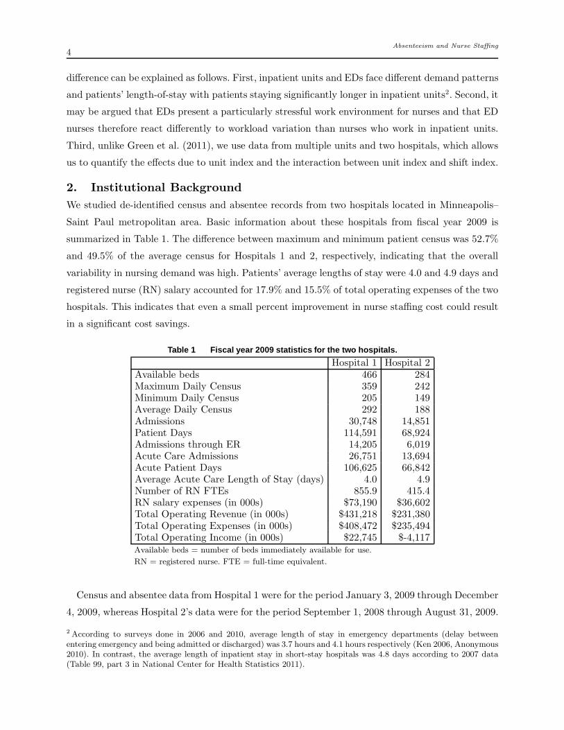
summarized in Table 1. The difference between maximum and minimum patient census was 52.7%
and 49.5% of the average census for Hospitals 1 and 2, respectively, indicating that the overall
variability in nursing demand was high. Patients’ average lengths of stay were 4.0 and 4.9 days and
registered nurse (RN) salary accounted for 17.9% and 15.5% of total operating expenses of the two
hospitals. This indicates that even a small percent improvement in nurse staffing cost could result
in a significant cost savings.
Table 1 Fiscal year 2009 statistics for the two hospitals.
Hospital 1 Hospital 2Available beds 466 284Maximum Daily Census 359 242Minimum Daily Census 205 149Average Daily Census 292 188Admissions 30,748 14,851Patient Days 114,591 68,924Admissions through ER 14,205 6,019Acute Care Admissions 26,751 13,694Acute Patient Days 106,625 66,842Average Acute Care Length of Stay (days) 4.0 4.9Number of RN FTEs 855.9 415.4RN salary expenses (in 000s) $73,190 $36,602Total Operating Revenue (in 000s) $431,218 $231,380Total Operating Expenses (in 000s) $408,472 $235,494Total Operating Income (in 000s) $22,745 $-4,117Available beds = number of beds immediately available for use.
RN = registered nurse. FTE = full-time equivalent.
Census and absentee data from Hospital 1 were for the period January 3, 2009 through December
4, 2009, whereas Hospital 2’s data were for the period September 1, 2008 through August 31, 2009.
2 According to surveys done in 2006 and 2010, average length of stay in emergency departments (delay betweenentering emergency and being admitted or discharged) was 3.7 hours and 4.1 hours respectively (Ken 2006, Anonymous2010). In contrast, the average length of inpatient stay in short-stay hospitals was 4.8 days according to 2007 data(Table 99, part 3 in National Center for Health Statistics 2011).
Absenteeism and Nurse Staffing5
Hospital 1 had five shift types. There were three 8-hour shifts designated Day, Evening, and Night
shifts, which operated from 7 AM to 3 PM, from 3 PM to 11 PM, and from 11 PM to 7 AM,
respectively. There were also two 12-hour shifts, which were designated Day-12 and Night-12 shifts.
These operated from 7 AM to 7 PM, and 7 PM to 7 AM, respectively. Hospital 2 had only three
shift types, namely the 8-hour Day, Evening, and Night shifts. Hospital 1’s data pertained to three
step-down (telemetry) units labeled T1, T2, and T3 with 22, 22, and 24 beds, and Hospital 2’s data
pertained to two medical/surgical units labeled M1 and M2 with 32 and 31 beds. The common data
elements were hourly census, hourly admissions discharges and transfers (ADT), planned/realized
staffing levels, and the count of absentees for each shift. Hospital 1’s data also contained individual
nurses’ attendance history. The two health systems’ data were analyzed independently because (1)
the data pertained to different time periods, (2) the target nurse-to-patient ratios were different
for the two types of nursing units, and (3) the two hospitals used different staffing strategies.
Hospital 1’s target nurse-to-patient ratios for telemetry units were 1:3 for Day and Evening shifts
during week days and 1:4 for Night and weekend shifts. Hospital 2’s target nurse-to-patient ratios
for medical/surgical units were 1:4 for Day and Evening shifts and 1:5 for Night shifts. Hospital
1’s planned staffing levels were based on the mode of the midnight census in the previous planning
period. Nurse managers would further tweak the staffing levels up or down to account for holidays
and to meet nurses’ planned-time-off requests and shift preferences. Hospital 2’s medical/surgical
units had fixed staffing levels based on the long-run average patient census by day of week and
shift. In both cases, staff planning was done in 4-week increments and planned staffing levels were
posted 2-weeks in advance of the first day of each 4-week plan. Consistent with the fact that average
lengths of stay in these hospitals were between 4 and 5 days, staffing levels were not based on a
projection of short-term demand forecast. When the number of patients exceeded the target nurse-
to-patient ratios, nurse managers attempted to increase staffing by utilizing extra-time or overtime
shifts, or calling in agency nurses. Similarly, when census was less than anticipated, nurses were
assigned to indirect patient care tasks or education activities, or else asked to take voluntary time
off. These efforts were not always successful and realized nurse-to-patient ratios often differed from
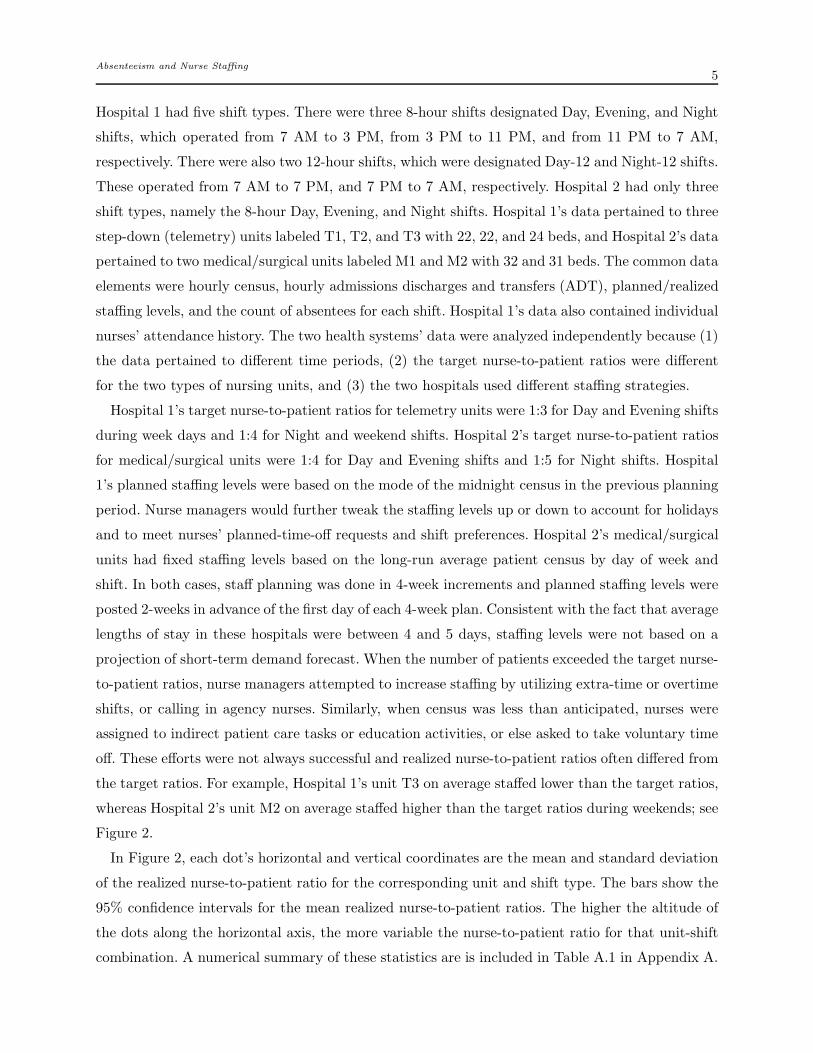
the target ratios. For example, Hospital 1’s unit T3 on average staffed lower than the target ratios,
whereas Hospital 2’s unit M2 on average staffed higher than the target ratios during weekends; see
Figure 2.
In Figure 2, each dot’s horizontal and vertical coordinates are the mean and standard deviation
of the realized nurse-to-patient ratio for the corresponding unit and shift type. The bars show the
95% confidence intervals for the mean realized nurse-to-patient ratios. The higher the altitude of
the dots along the horizontal axis, the more variable the nurse-to-patient ratio for that unit-shift
combination. A numerical summary of these statistics are is included in Table A.1 in Appendix A.
Absenteeism and Nurse Staffing6
Figure 2 Average Number of Patients Per Nurse by Shift Type
2.5 3.0 3.5 4.0 4.5 5.0
0.4
0.6
0.8
1.0
1.2
1.4
Avg Number of Patients Per Nurse
SD
of N
umbe
r of
Pat
ient
s P
er N
urse
T1 (D/E)
T2 (D/E)
T3 (D/E)
T1 (N)
T2 (N)
T3 (N)
M1 (D/E)M2 (D/E)
M1 (N)
M2 (N)
TR 1 TR 2 TR 3
Note: D = Day. E = Evening. N = Night. TR 1 = Target ratio for T1, T2, and T3 in D and E shifts during weekdays.TR 2 = Target ratio for T1, T2, and T3 in N shifts or weekends; TR 2 is also the target ratio for M1 and M2 in Dand E Shifts. TR 3 = Target ratio for M1 and M2 in N shifts.
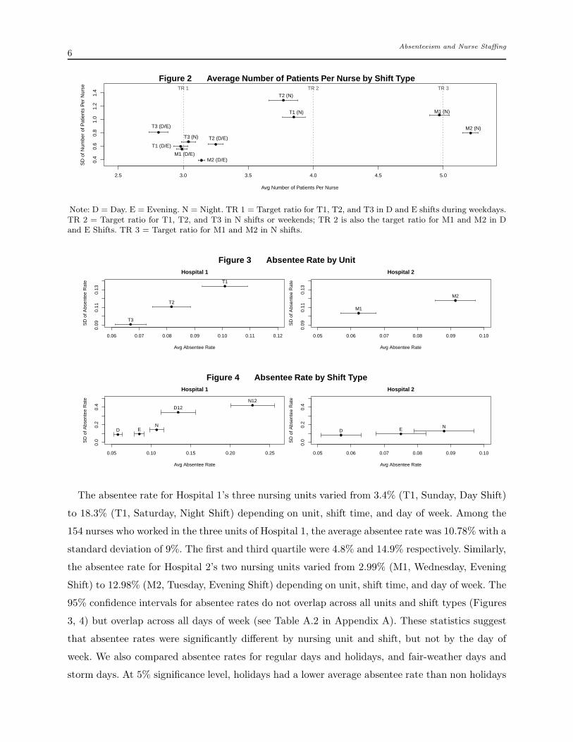
Figure 3 Absentee Rate by Unit
0.06 0.07 0.08 0.09 0.10 0.11 0.12
0.09
0.11
0.13
Hospital 1
Avg Absentee Rate
SD
of A
bsen
tee
Rat
e T1
T2
T3
0.05 0.06 0.07 0.08 0.09 0.10
0.09
0.11
0.13
Hospital 2
Avg Absentee Rate
SD
of A
bsen
tee
Rat
e
M1
M2
Figure 4 Absentee Rate by Shift Type
0.05 0.10 0.15 0.20 0.25
0.0
0.2
0.4
Hospital 1
Avg Absentee Rate
SD
of A
bsen
tee
Rat
e
D EN
D12
N12
0.05 0.06 0.07 0.08 0.09 0.10
0.0
0.2
0.4
Hospital 2
Avg Absentee Rate
SD
of A
bsen
tee
Rat
e
D E N
The absentee rate for Hospital 1’s three nursing units varied from 3.4% (T1, Sunday, Day Shift)
to 18.3% (T1, Saturday, Night Shift) depending on unit, shift time, and day of week. Among the
154 nurses who worked in the three units of Hospital 1, the average absentee rate was 10.78% with a
standard deviation of 9%. The first and third quartile were 4.8% and 14.9% respectively. Similarly,
the absentee rate for Hospital 2’s two nursing units varied from 2.99% (M1, Wednesday, Evening
Shift) to 12.98% (M2, Tuesday, Evening Shift) depending on unit, shift time, and day of week. The
95% confidence intervals for absentee rates do not overlap across all units and shift types (Figures
3, 4) but overlap across all days of week (see Table A.2 in Appendix A). These statistics suggest
that absentee rates were significantly different by nursing unit and shift, but not by the day of
week. We also compared absentee rates for regular days and holidays, and fair-weather days and
storm days. At 5% significance level, holidays had a lower average absentee rate than non holidays
Absenteeism and Nurse Staffing7
for Hospital 2 and storm days had a higher average absentee rate for Hospital 1. A numerical
summary of absentee rates is included in Table A.2 in Appendix A.
3. Statistical Models & Results
We next present two models to evaluate different predictors of nurse absenteeism. The choice of
potential predictors was based on interactions with nurse managers and findings in previous studies.
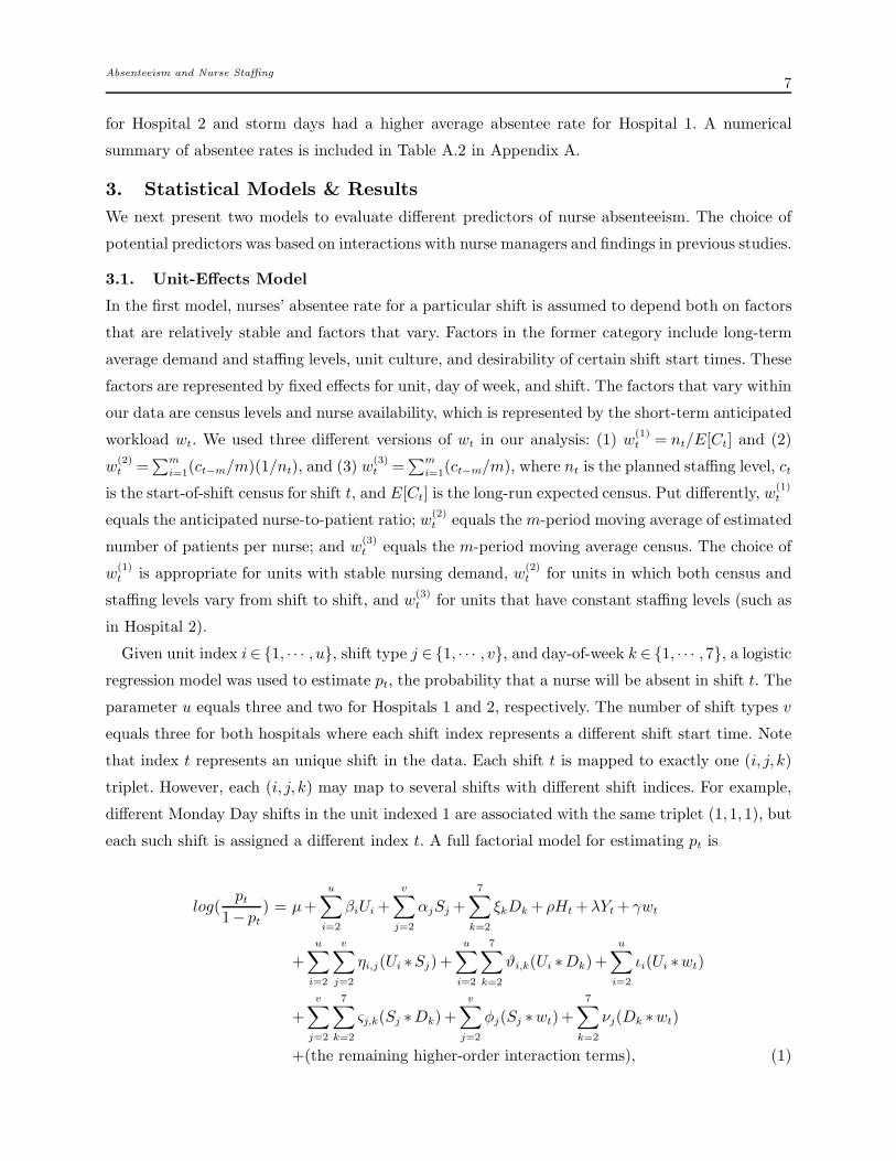
3.1. Unit-Effects Model
In the first model, nurses’ absentee rate for a particular shift is assumed to depend both on factors
that are relatively stable and factors that vary. Factors in the former category include long-term
average demand and staffing levels, unit culture, and desirability of certain shift start times. These
factors are represented by fixed effects for unit, day of week, and shift. The factors that vary within
our data are census levels and nurse availability, which is represented by the short-term anticipated
workload wt. We used three different versions of wt in our analysis: (1) w(1)t = nt/E[Ct] and (2)
w(2)t =
∑m
i=1(ct−m/m)(1/nt), and (3) w(3)t =
∑m
i=1(ct−m/m), where nt is the planned staffing level, ct
is the start-of-shift census for shift t, and E[Ct] is the long-run expected census. Put differently, w(1)t
equals the anticipated nurse-to-patient ratio; w(2)t equals the m-period moving average of estimated
number of patients per nurse; and w(3)t equals the m-period moving average census. The choice of
w(1)t is appropriate for units with stable nursing demand, w
(2)t for units in which both census and
staffing levels vary from shift to shift, and w(3)t for units that have constant staffing levels (such as
in Hospital 2).
Given unit index i∈ {1, · · · , u}, shift type j ∈ {1, · · · , v}, and day-of-week k ∈ {1, · · · ,7}, a logistic
regression model was used to estimate pt, the probability that a nurse will be absent in shift t. The
parameter u equals three and two for Hospitals 1 and 2, respectively. The number of shift types v
equals three for both hospitals where each shift index represents a different shift start time. Note
that index t represents an unique shift in the data. Each shift t is mapped to exactly one (i, j, k)
triplet. However, each (i, j, k) may map to several shifts with different shift indices. For example,
different Monday Day shifts in the unit indexed 1 are associated with the same triplet (1,1,1), but
each such shift is assigned a different index t. A full factorial model for estimating pt is
log(pt
1− pt) = µ+
u∑
i=2
βiUi +v
∑
j=2
αjSj +7
∑
k=2
ξkDk + ρHt +λYt + γwt
+u
∑
i=2
v∑
j=2
ηi,j(Ui ∗Sj)+u
∑
i=2
7∑
k=2
ϑi,k(Ui ∗Dk)+u
∑
i=2
ιi(Ui ∗wt)
+v
∑
j=2
7∑
k=2
ςj,k(Sj ∗Dk)+v
∑
j=2
φj(Sj ∗wt)+7
∑
k=2
νj(Dk ∗wt)
+(the remaining higher-order interaction terms), (1)

Absenteeism and Nurse Staffing8
where Ui, Sj, and Dk are indicator variables. In particular, Ui = 1 if the nurse under evaluation
worked in unit i and Ui = 0 otherwise. Similarly, Sj = 1 (respectively Dk = 1) if the nurse was
scheduled to work on a type-j shift (respectively day k of the week). Ht and Yt are also indicator
variables that are set equal to 1 if shift t occurred on either a holiday or a bad-weather day. The
unit, shift, and day-of-week with the smallest indices are used as the benchmark group in the above
model. We use (a∗b) to denote the interaction term of a and b. In the ensuing analysis, all two-way
interactions are included in the initial model but higher-order interaction terms are omitted. This
is done because higher order interaction terms do not have a practical interpretation (see Faraway
2006 for supporting arguments). Notation and assumptions are summarized in Table 2.
Table 2 Unit-Effects Model Notation and Assumptions
Covariate Description Coefficientpt absentee rate for a shift t noneUi indicator variable for unit i. βi
Sj indicator variable for shift type j αj
Dk indicator variable for day k of the week ξkHt indicator variable for holiday shifts ρYt indicator variable for storm-day shifts λwt short-term anticipated workload for shift t γ
(Ui ∗Sj) unit and shift interaction ηi,j(Ui ∗Dk) unit and day of week interaction ϑi,k
(Ui ∗wt) unit and workload interaction ιi(Sj ∗Dk) shift and day of week interaction ςj,k(Sj ∗wt) shift and workload interaction φj
(Dk ∗wt) day of week and workload interaction νjAssumptions:
1. Independent and homogeneous nurses.
2. A nurse’s attendance decision for a particular shift is independent of his/her decisions for other shifts.
The explanatory variables in (1) capture the systematic variation in nurses’ absentee rates due
to unit, shift time, day of week, and their interactions. Because long-term workload is included in
these factors, we did not include that as a separate predictor. We also decided not to include week-
or month-of-year effect because of data limitations3.
We used stepwise variable selection processes to leave out insignificant explanatory factors by
comparing nested models’ deviances via Chi-square tests. Only factors that significantly improved
model fits at the 5% significance level were retained in the model. A summary of our results with
3 With approximately 1 year of data, observations of higher/lower absentee rate in certain weeks are not informativeabout future absentee rates in those weeks. Also, when week of year was included as an explanatory variable, thisresulted in some covariate classes with too few observations. For example, there were only 3 nurses who were scheduledto work during week 2 (the week of 1/4/09 – 1/10/09) Monday Night shift in Unit 1 of Hospital 1.
Absenteeism and Nurse Staffing9
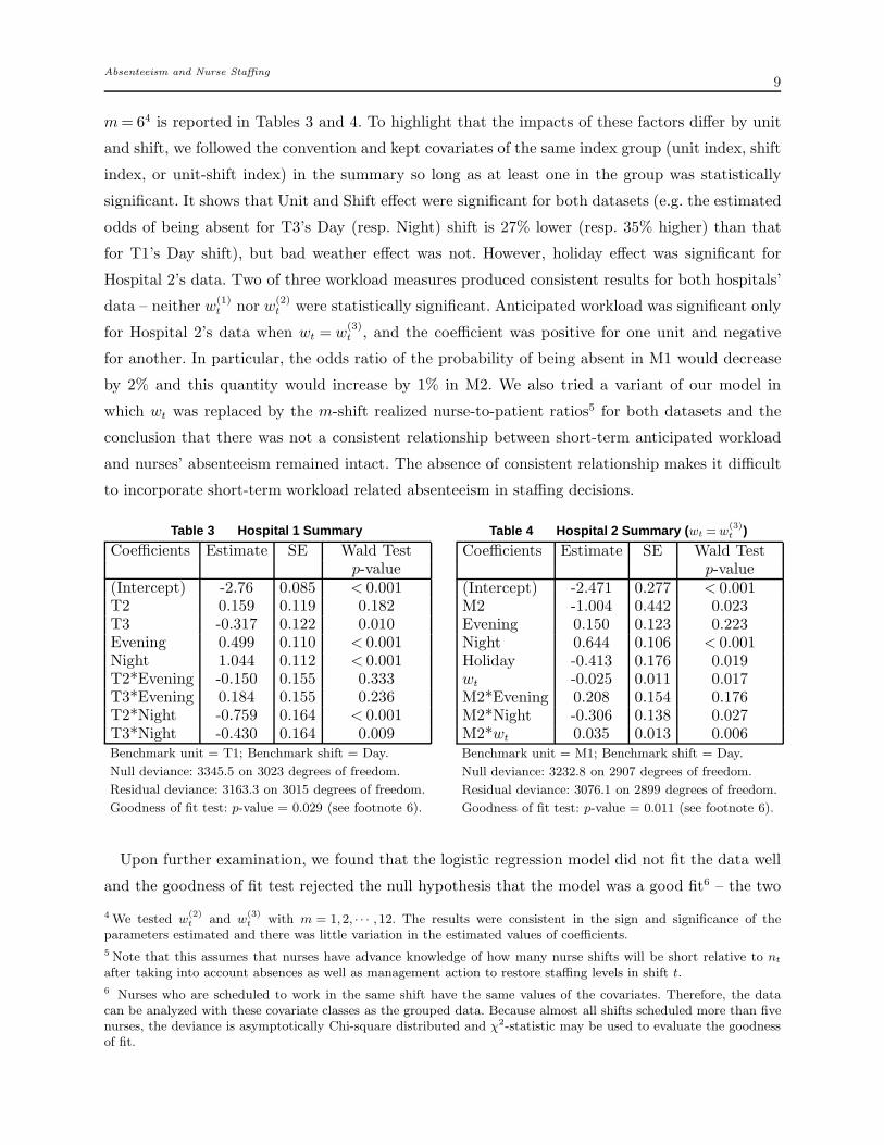
m= 64 is reported in Tables 3 and 4. To highlight that the impacts of these factors differ by unit
and shift, we followed the convention and kept covariates of the same index group (unit index, shift
index, or unit-shift index) in the summary so long as at least one in the group was statistically
significant. It shows that Unit and Shift effect were significant for both datasets (e.g. the estimated
odds of being absent for T3’s Day (resp. Night) shift is 27% lower (resp. 35% higher) than that
for T1’s Day shift), but bad weather effect was not. However, holiday effect was significant for
Hospital 2’s data. Two of three workload measures produced consistent results for both hospitals’
data – neither w(1)t nor w(2)
t were statistically significant. Anticipated workload was significant only
for Hospital 2’s data when wt = w(3)t , and the coefficient was positive for one unit and negative
for another. In particular, the odds ratio of the probability of being absent in M1 would decrease
by 2% and this quantity would increase by 1% in M2. We also tried a variant of our model in
which wt was replaced by the m-shift realized nurse-to-patient ratios5 for both datasets and the
conclusion that there was not a consistent relationship between short-term anticipated workload
and nurses’ absenteeism remained intact. The absence of consistent relationship makes it difficult
to incorporate short-term workload related absenteeism in staffing decisions.
Table 3 Hospital 1 Summary
Coefficients Estimate SE Wald Testp-value
(Intercept) -2.76 0.085 < 0.001T2 0.159 0.119 0.182T3 -0.317 0.122 0.010Evening 0.499 0.110 < 0.001Night 1.044 0.112 < 0.001T2*Evening -0.150 0.155 0.333T3*Evening 0.184 0.155 0.236T2*Night -0.759 0.164 < 0.001T3*Night -0.430 0.164 0.009Benchmark unit = T1; Benchmark shift = Day.
Null deviance: 3345.5 on 3023 degrees of freedom.
Residual deviance: 3163.3 on 3015 degrees of freedom.
Goodness of fit test: p-value = 0.029 (see footnote 6).
Table 4 Hospital 2 Summary ( wt =w(3)t )
Coefficients Estimate SE Wald Testp-value
(Intercept) -2.471 0.277 < 0.001M2 -1.004 0.442 0.023Evening 0.150 0.123 0.223Night 0.644 0.106 < 0.001Holiday -0.413 0.176 0.019wt -0.025 0.011 0.017M2*Evening 0.208 0.154 0.176M2*Night -0.306 0.138 0.027M2*wt 0.035 0.013 0.006Benchmark unit = M1; Benchmark shift = Day.
Null deviance: 3232.8 on 2907 degrees of freedom.
Residual deviance: 3076.1 on 2899 degrees of freedom.
Goodness of fit test: p-value = 0.011 (see footnote 6).
Upon further examination, we found that the logistic regression model did not fit the data well
and the goodness of fit test rejected the null hypothesis that the model was a good fit6 – the two
4 We tested w(2)t
and w(3)t
with m = 1,2, · · · ,12. The results were consistent in the sign and significance of theparameters estimated and there was little variation in the estimated values of coefficients.
5 Note that this assumes that nurses have advance knowledge of how many nurse shifts will be short relative to nt
after taking into account absences as well as management action to restore staffing levels in shift t.
6 Nurses who are scheduled to work in the same shift have the same values of the covariates. Therefore, the datacan be analyzed with these covariate classes as the grouped data. Because almost all shifts scheduled more than fivenurses, the deviance is asymptotically Chi-square distributed and χ2-statistic may be used to evaluate the goodnessof fit.
Absenteeism and Nurse Staffing10
models in Tables 2 and 3 respectively resulted in a p-value of 0.029 and 0.011. This happened
because of the large residual deviances of the unit-level model. The lack of fit may be caused by a
variety of reasons. For example, it is possible that unit-level factors/covariates do not adequately
explain nurses’ absentee rates, or that overdispersion7 occurred due to non-constant probability
within a covariate class (e.g. population heterogeneity). It is also possible that the unit, shift, and
day of week patterns are confounded with individual nurses’ work patterns – some high absentee
rate nurses may have a fixed work pattern that contributed to the high absentee rates for some
shifts. Some nurses also changed their work patterns during the data collection period, which may
result in the large deviance if nurse-specific effects were strong.
One of the critical assumptions underlying the generalized linear model (GLM) in Equation
(1) is the statistical independence of observations; e.g. all observations, regardless of whether the
attendance records belong to the same or different nurses, are independent. This assumption may
not hold when there is a natural clustering of the data and possible intra-cluster correlation. If there
is a positive correlation among observations, the variance of the coefficients will be underestimated
upon ignoring the covariances and inferences for these coefficients may be inaccurate.
Hospital 1’s data are comprised of multiple observations of each nurse’s outcome (response)
variable (whether a nurse was absent or present for a scheduled shift) and a set of unit-level
covariates (e.g. unit index, shift time, day of week, workload, etc). Each nurse can be viewed as
a cluster with correlation among the observations (attendance outcomes) of a nurse. Therefore,
we also evaluated whether unit, shift, and day of week effects still exist after we accounted for
individual nurses’ effect. We used generalized estimating equations (GEE) to fit a repeated measure
logistic regression model with Hospital 1’s data. GEE, first introduced in Zeger and Liang (1986),
is a method for analyzing correlated data. Although there are other statistical methods that may
be used to evaluate repeated measures data (e.g. generalized linear mixed models, hierarchical
generalized linear models), we chose GEE approach because this method has a track record of being
useful in many applications and it has been implemented in several statistical packages (e.g. SAS,
SPSS, R).
We applied the GEE approach to estimate the effect of unit-level factors (see Equation (1)).
We estimated associations between outcomes of the same nurse ℓ, and assumed that outcomes of
different nurses are independent (i.e. nurses are still assumed to be independent decision makers).
The number of observations differed across nurses resulting in unbalanced data. We had observa-
tions for 160 nurses. The average number of observations per nurse was 107.44, and the standard
deviation of the number of shifts scheduled among these nurses was 52.23.
7 Overdispersion means that the variability around the model’s fitted value is higher than what is consistent with theformulated model.

Absenteeism and Nurse Staffing11
Table 5 Hospital 1 GEE Model Summary.
Coefficients Estimate SE Wald Testp-value
(Intercept) 2.455 0.185 < 0.0005T2 -0.015 0.205 0.942T3 0.243 0.215 0.259Evening -0.543 0.136 < 0.0005Night -0.736 0.193 < 0.0005Mon -0.095 0.124 0.443Tue 0.158 0.1232 0.199Wed 0.254 0.1202 0.035Thu 0.071 0.1055 0.501Fri 0.127 0.1197 0.29Sat -0.126 0.0956 0.188Benchmark unit = T1; Benchmark shift = Day;Benchmark day of week = Sunday.
The results in Table 5 show that shift effect and Wednesday’s day of week effect were significant
while accounting for individual nurses’ effect. However, unit effect was no longer significant. This
observation was different from the model in which we assumed independent and homogeneous
nurses. The differences in results from the GLM and GEE models suggest that it is not reasonable
to ignore differences among nurses. Therefore, we next investigate a nurse-effects model and its
implications for staffing decisions.
3.2. Nurse-Effects Model
We divided Hospital 1’s staffing data into two periods – before and after June 30, 2009. There were
146 nurses who worked for more than 10 shifts in both periods. Paired sample t-test showed that
the average absentee rate did not change across these two periods, which indicates an overall stable
absentee rate. Among these nurses, we calculated the absentee rate prior to June 30, 2009 for each
nurse. The mean and median absentee rates among those nurses were 11.0% and 7.6%, respectively,
and the standard deviation was 12.0%. For both time periods, we identified nurses whose absentee
rates were higher (resp. lower) than 7.6% during the period and categorized these nurses as type-
1 (resp. type-2) nurses for that period. The Phi coefficient was 0.43 with the two-by-two nurse
classification for the two periods, which indicated a positive association between nurse types –
nurses who were categorized as a particular type in period 1 were more likely to be categorized
as the same type in period 2. For each shift, we model the impact of nurse-effects via the percent
of type-1 nurses scheduled for that shift. We used the data between July 1st and December 4th,
2009 to evaluate the impact of having different proportions of period 1 type-1 nurses scheduled for
a shift. We fitted the following model:
Absenteeism and Nurse Staffing12
log(pt
1− pt) = µ+
u∑
i=2
βiUi +v
∑
j=2
αjSj +7
∑
k=2
ξkDk + γwt + νzt +(two-way interaction terms),
(2)
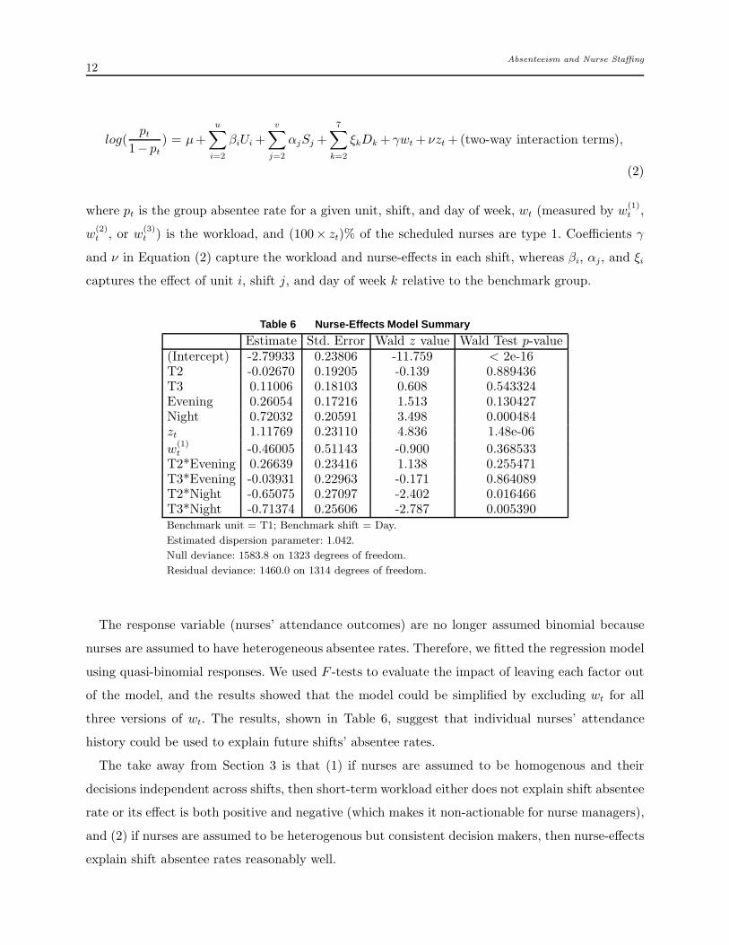
where pt is the group absentee rate for a given unit, shift, and day of week, wt (measured by w(1)t ,
w(2)t , or w
(3)t ) is the workload, and (100× zt)% of the scheduled nurses are type 1. Coefficients γ
and ν in Equation (2) capture the workload and nurse-effects in each shift, whereas βi, αj, and ξi
captures the effect of unit i, shift j, and day of week k relative to the benchmark group.
Table 6 Nurse-Effects Model Summary
Estimate Std. Error Wald z value Wald Test p-value(Intercept) -2.79933 0.23806 -11.759 < 2e-16T2 -0.02670 0.19205 -0.139 0.889436T3 0.11006 0.18103 0.608 0.543324Evening 0.26054 0.17216 1.513 0.130427Night 0.72032 0.20591 3.498 0.000484zt 1.11769 0.23110 4.836 1.48e-06
w(1)t -0.46005 0.51143 -0.900 0.368533
T2*Evening 0.26639 0.23416 1.138 0.255471T3*Evening -0.03931 0.22963 -0.171 0.864089T2*Night -0.65075 0.27097 -2.402 0.016466T3*Night -0.71374 0.25606 -2.787 0.005390Benchmark unit = T1; Benchmark shift = Day.
Estimated dispersion parameter: 1.042.
Null deviance: 1583.8 on 1323 degrees of freedom.
Residual deviance: 1460.0 on 1314 degrees of freedom.
The response variable (nurses’ attendance outcomes) are no longer assumed binomial because
nurses are assumed to have heterogeneous absentee rates. Therefore, we fitted the regression model
using quasi-binomial responses. We used F -tests to evaluate the impact of leaving each factor out
of the model, and the results showed that the model could be simplified by excluding wt for all
three versions of wt. The results, shown in Table 6, suggest that individual nurses’ attendance
history could be used to explain future shifts’ absentee rates.
The take away from Section 3 is that (1) if nurses are assumed to be homogenous and their
decisions independent across shifts, then short-term workload either does not explain shift absentee
rate or its effect is both positive and negative (which makes it non-actionable for nurse managers),
and (2) if nurses are assumed to be heterogenous but consistent decision makers, then nurse-effects
explain shift absentee rates reasonably well.

Absenteeism and Nurse Staffing13
4. Motivating Examples
Nurse managers routinely make staffing decisions that affect a hospital’s total staffing costs, nurses’
job satisfaction, and patients’ quality of care and safety. In this section, we present two examples
to highlight the importance of paying attention to heterogeneous absentee rates. The first example
concerns a decision that arises periodically. In this scenario, nurse managers need to assign nurses
with similar skills to inpatient units with similar requirements either to rebalance workload or
in response to reorganization of beds and change in patient volumes. Suppose nurses need to be
assigned to two inpatient units with independent Poisson distributed demand with a mean of 4
nurses per shift. Ten nurses with absentee rates (0.6, 0.6, 0.2, 0.2, 0.2, 0.2, 0, 0, 0, 0) are available.
Nurse skills are such that each nurse can be assigned to any one of the two units. How should the
nurse manager assign nurses?
Intuitively, a nurse manager may wish to even the staffing level. Consider two staffing strategies
that both utilize all 10 nurses: (1) 6 nurses with absentee rates (0.6, 0.6, 0.2, 0.2, 0.2, 0.2) are
assigned to Unit 1 and 4 nurses with zero absentee rates are assigned to Unit 2; and (2) two
identical groups of 5 nurses each with absentee rates (0.6, 0.2, 0.2, 0, 0) are assigned to each unit.
The expected number of nurses who show up in a shift in each unit is 4 in both these arrangements.
However, it can be shown that the average number of shifts short in Unit 1 is only 48.2% of that in
Unit 2 under the first plan. In addition, the average number of shifts short across both units under
the first plan is 103% higher than the second plan. The first plan assigns nurses in a manner that
the first unit is quite different from the second unit, whereas the second plan creates an identical
assignment across the two units. It is natural to ask whether the insights from this example are
generalizable. Is there is a strategy to allocate available nurses based on their absentee rates that
minimizes the expected shortage cost? We partially address this question in the next section.
The second example concerns a situation that arises more frequently. Nurse managers often
find out a few shifts before a particular shift that they might face a staff shortage in that shift.
Such assessments are based on inpatients’ health status, scheduled admissions, and anticipated
discharges. Nurse managers like to recruit part-time nurses to work extra shifts to satisfy the excess
demand. This is cheaper and less stressful than finding overtime or agency nurses at a short notice.
In hospitals with unionized workforce, nurse managers need to announce the opportunity to pick
up extra shifts to all nurses who are qualified for these shifts, and union rules may dictate the
order in which extra shift requests must be granted; e.g. Hospital 1 is required to prioritize such
requests by seniority. Consequently, nurse managers have little control over who may be selected
to work extra shifts. When nurses absentee rates are different, the determination of the number of
extra shifts (or target staffing level) becomes difficult.
Absenteeism and Nurse Staffing14
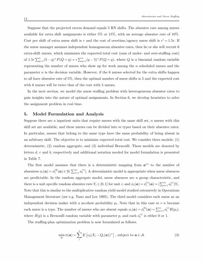
Suppose that the projected excess demand equals 5 RN shifts. The absentee rate among nurses
available for extra shift assignments is either 5% or 15%, with an average absentee rate of 10%.
Cost per shift of extra nurse shift is r and the cost of overtime/agency nurse shift is r′ = 1.5r. If
the nurse manager assumes independent homogeneous absentee rates, then he or she will recruit 6
extra-shift nurses, which minimizes the expected total cost (sum of under- and over-staffing cost)
of 1.5r∑n
q=1(5− q)+P (Q= q) + r∑n
q=1(q− 5)+P (Q= q), where Q is a binomial random variable
representing the number of nurses who show up for work among the n scheduled nurses and the
parameter n is the decision variable. However, if the 6 nurses selected for the extra shifts happen
to all have absentee rate of 5%, then the optimal number of nurse shifts is 5 and the expected cost
with 6 nurses will be twice that of the cost with 5 nurses.
In the next section, we model the nurse staffing problem with heterogeneous absentee rates to
gain insights into the nature of optimal assignments. In Section 6, we develop heuristics to solve
the assignment problem in real time.
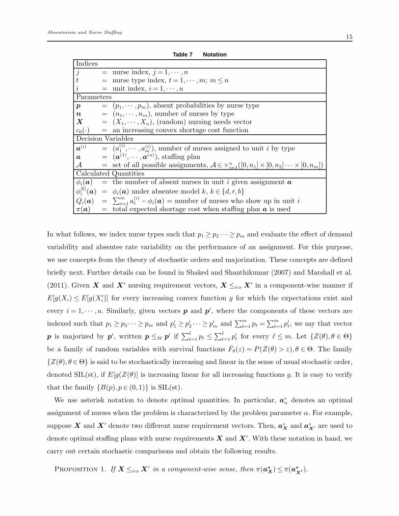
5. Model Formulation and Analysis
Suppose there are u inpatient units that require nurses with the same skill set, n nurses with this
skill set are available, and these nurses can be divided into m types based on their absentee rates.
In particular, nurses that belong to the same type have the same probability of being absent in
an arbitrary shift. The objective is to minimize expected total cost. We consider three models: (1)
deterministic, (2) random aggregate, and (3) individual Bernoulli. These models are denoted by
letters d, r and b, respectively and additional notation needed for model formulation is presented
in Table 7.
The first model assumes that there is a deterministic mapping from a(i) to the number of
absentees φi(a) = φ[d]i (a)∈ [0,
∑m
t=1 a(i)t ]. A deterministic model is appropriate when nurse absences
are predictable. In the random aggregate model, nurse absences are a group characteristic, and
there is a unit specific random absentee rate Yi ∈ [0,1] for unit i, and φi(a) = φ[r]i (a) = (
∑m
t=1 a(i)t )Yi.
Note that this is similar to the multiplicative random yield model studied extensively in Operations
Management literature (see e.g. Yano and Lee 1995). The third model considers each nurse as an
independent decision maker with a no-show probability pt. Note that in this case m= n because
each nurse is a type. The number of nurses who are absent equals φi(a) = φ[b]i (a) =
∑n
t=1 a(i)t B(pt),
where B(p) is a Bernoulli random variable with parameter p, and each a(i)t is either 0 or 1.
The staffing-plan optimization problem is now formulated as follows.
mina
π(a) =u
∑
i
E[
c0(Xi−Qi(a))+]
, subject to a∈A. (3)
Absenteeism and Nurse Staffing15
Table 7 Notation
Indicesj = nurse index, j =1, · · · , nt = nurse type index, t= 1, · · · ,m; m≤ ni = unit index, i= 1, · · · , uParametersp = (p1, · · · , pm), absent probabilities by nurse typen = (n1, · · · , nm), number of nurses by typeX = (X1, · · · ,Xu), (random) nursing needs vectorc0(·) = an increasing convex shortage cost functionDecision Variables
a(i) = (a(i)1 , · · · , a(i)
m ), number of nurses assigned to unit i by typea = (a(1), · · · ,a(u)), staffing planA = set of all possible assignments, A∈×u
i=1([0, n1]× [0, n2] · · · × [0, nm])Calculated Quantitiesφi(a) = the number of absent nurses in unit i given assignment a
φ[k]i (a) = φi(a) under absentee model k, k ∈ {d, r, b}
Qi(a) =∑m
t=1 a(i)t −φi(a) = number of nurses who show up in unit i
π(a) = total expected shortage cost when staffing plan a is used
In what follows, we index nurse types such that p1 ≥ p2 · · · ≥ pm and evaluate the effect of demand
variability and absentee rate variability on the performance of an assignment. For this purpose,
we use concepts from the theory of stochastic orders and majorization. These concepts are defined
briefly next. Further details can be found in Shaked and Shanthikumar (2007) and Marshall et al.
(2011). Given X and X ′ nursing requirement vectors, X ≤icx X′ in a component-wise manner if
E[g(Xi) ≤ E[g(X ′
i)] for every increasing convex function g for which the expectations exist and
every i = 1, · · · , u. Similarly, given vectors p and p′, where the components of these vectors are
indexed such that p1 ≥ p2 · · · ≥ pm and p′1 ≥ p′2 · · · ≥ p′m and∑m
t=1 pt =∑m
t=1 p′
t, we say that vector
p is majorized by p′, written p ≤M p′ if∑ℓ
t=1 pt ≤∑ℓ
t=1 p′
t for every ℓ ≤ m. Let {Z(θ), θ ∈ Θ}
be a family of random variables with survival functions Fθ(z) = P (Z(θ)> z), θ ∈ Θ. The family
{Z(θ), θ ∈Θ} is said to be stochastically increasing and linear in the sense of usual stochastic order,
denoted SIL(st), if E[g(Z(θ)] is increasing linear for all increasing functions g. It is easy to verify
that the family {B(p), p∈ (0,1)} is SIL(st).
We use asterisk notation to denote optimal quantities. In particular, a∗
α denotes an optimal
assignment of nurses when the problem is characterized by the problem parameter α. For example,
suppose X and X ′ denote two different nurse requirement vectors. Then, a∗
Xand a∗
X′ are used to
denote optimal staffing plans with nurse requirements X and X ′. With these notation in hand, we
carry out certain stochastic comparisons and obtain the following results.
Proposition 1. If X ≤icx X′ in a component-wise sense, then π(a∗
X)≤ π(a∗
X′).

Absenteeism and Nurse Staffing16
Proposition 1 states that larger and more variable demand leads to greater expected shortage costs.
This statement applies for all three models. The proof of Proposition 1 is included in Appendix
B. The result in Proposition 1 is intuitive because for a fixed level of available staff, shortage costs
increase when demand is either greater or more uncertain.
Proposition 2. Let φi(a) = φ[d]i (a) be a deterministic mapping from a(i) to [0,
∑m
t=1 a(i)t ]. If
{Xi} are independent and identically distributed (i.i.d.), then an optimal staffing plan is realized
upon making Qi(a∗) equal for all i= 1, · · · ,m.
Proposition 2 states that if absenteeism can be predicted reasonably well and inpatient units have
i.i.d. demand, then the nurse manager should assign nurses such that each unit has the same
realized staffing level. A proof of Proposition 2 is presented in Appendix B.
Proposition 3. Let φi(a) =∑m
t=1 a(i)t Yi, where Yi ∈ [0,1] is the random unit-level absentee rate
for unit i and Y = (Y1, · · · , Yu). If Y ≤icx Y′ in a component-wise manner, then π(a∗
Y )≤ π(a∗
Y ′).
Proposition 3 shows that if nurses are homogenous, then a nurse manager would prefer a cohort of
nurses with a stochastically smaller absentee rate (i.e. nurses with smaller mean and/or variance
of aggregate absentee rate). See Appendix B for the proof of Proposition 3. However, this does not
hold when nurses are heterogenous, as shown in Proposition 4.
The next result applies to each unit considered separately. For this purpose, we define p(i) to
be the absentee probabilities of nurses assigned to unit i. That is, components of p(i) contain
information about only those nurses that are assigned to unit i. Furthermore, let πi(p(i)) denote the
expected shortage cost incurred in unit i with no-show probability vector p(i). Then, with individual
Bernoulli no-show model, we can prove that a nurse manager would prefer a more variable mix of
absentee rates.
Proposition 4. If p(i) ≤M p′(i), then πi(p′)≤ πi(p).
Proposition 4 shows that for a given staffing plan, the nurse manager would prefer to utilize a more
heterogeneous cohort of nurses. However, this may not be the best overall strategy when costs
across different units need to be balanced. It is the difficulty of balancing staffing across units while
maximizing heterogeneity within a unit that makes it difficult to identify an optimal assignment
strategy. A proof of Proposition 4 is included in Appendix B.
Propositions 2 and 4 can be used to explain observations in the first example of Section 4. We
considered two staffing strategies. Both were consistent with Proposition 2 and maintained the
same expected number of nurses who show up in each unit. The absentee rate of nurse assigned to
Unit 2 under the first strategy can be written as (1,0,0,0,0). That is, adding a nurse who never
shows up makes no difference. Clearly, this majorizes the absentee rate vector (0.6,0.2,0.2,0,0) of
Absenteeism and Nurse Staffing17
assignments made under strategy 2 and Unit 2 performs better under strategy 1. However, upon
writing Unit 1’s assignment under strategy 2 as having the absentee rate vector (1,0.6,0.2,0.2,0,0),
we find that this assignment majorizes Unit 1’s assignment under strategy 1. That is, Unit 1
performs better under strategy 2. Finally, strategy 2 emerges as the overall best choice because
the two units are identical and shortage costs are increasing convex. The take away from this
section is that in addition to reducing demand variability, hospitals can also benefit from staffing
similar inpatient units in a way such that the absentee rates are heterogeneous within a unit but
homogeneous across units.
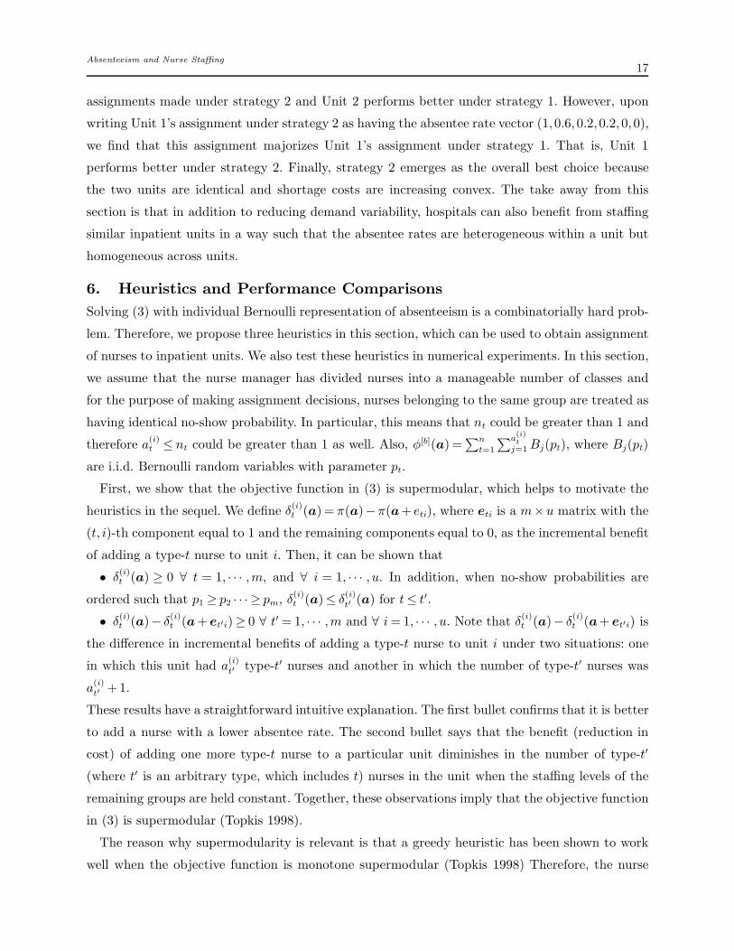
6. Heuristics and Performance Comparisons
Solving (3) with individual Bernoulli representation of absenteeism is a combinatorially hard prob-
lem. Therefore, we propose three heuristics in this section, which can be used to obtain assignment
of nurses to inpatient units. We also test these heuristics in numerical experiments. In this section,
we assume that the nurse manager has divided nurses into a manageable number of classes and
for the purpose of making assignment decisions, nurses belonging to the same group are treated as
having identical no-show probability. In particular, this means that nt could be greater than 1 and
therefore a(i)t ≤ nt could be greater than 1 as well. Also, φ[b](a) =
∑n
t=1
∑a(i)t
j=1Bj(pt), where Bj(pt)
are i.i.d. Bernoulli random variables with parameter pt.
First, we show that the objective function in (3) is supermodular, which helps to motivate the
heuristics in the sequel. We define δ(i)t (a) = π(a)−π(a+ eti), where eti is a m×u matrix with the
(t, i)-th component equal to 1 and the remaining components equal to 0, as the incremental benefit
of adding a type-t nurse to unit i. Then, it can be shown that
• δ(i)t (a) ≥ 0 ∀ t = 1, · · · ,m, and ∀ i = 1, · · · , u. In addition, when no-show probabilities are
ordered such that p1 ≥ p2 · · · ≥ pm, δ(i)t (a)≤ δ
(i)
t′(a) for t≤ t′.
• δ(i)t (a)− δ
(i)t (a+et′i)≥ 0 ∀ t′ = 1, · · · ,m and ∀ i= 1, · · · , u. Note that δ
(i)t (a)− δ
(i)t (a+ et′i) is
the difference in incremental benefits of adding a type-t nurse to unit i under two situations: one
in which this unit had a(i)
t′type-t′ nurses and another in which the number of type-t′ nurses was
a(i)
t′+1.
These results have a straightforward intuitive explanation. The first bullet confirms that it is better
to add a nurse with a lower absentee rate. The second bullet says that the benefit (reduction in
cost) of adding one more type-t nurse to a particular unit diminishes in the number of type-t′
(where t′ is an arbitrary type, which includes t) nurses in the unit when the staffing levels of the
remaining groups are held constant. Together, these observations imply that the objective function
in (3) is supermodular (Topkis 1998).
The reason why supermodularity is relevant is that a greedy heuristic has been shown to work
well when the objective function is monotone supermodular (Topkis 1998) Therefore, the nurse
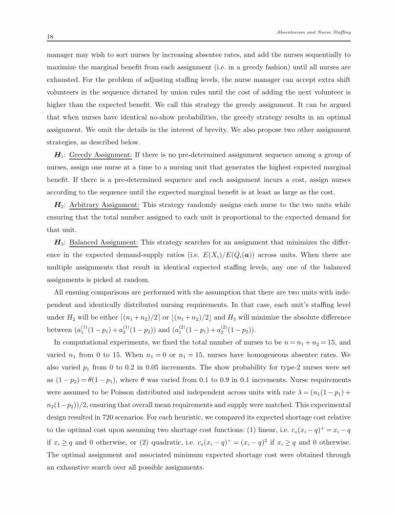
Absenteeism and Nurse Staffing18
manager may wish to sort nurses by increasing absentee rates, and add the nurses sequentially to
maximize the marginal benefit from each assignment (i.e. in a greedy fashion) until all nurses are
exhausted. For the problem of adjusting staffing levels, the nurse manager can accept extra shift
volunteers in the sequence dictated by union rules until the cost of adding the next volunteer is
higher than the expected benefit. We call this strategy the greedy assignment. It can be argued
that when nurses have identical no-show probabilities, the greedy strategy results in an optimal
assignment. We omit the details in the interest of brevity. We also propose two other assignment
strategies, as described below.
H1: Greedy Assignment: If there is no pre-determined assignment sequence among a group of
nurses, assign one nurse at a time to a nursing unit that generates the highest expected marginal
benefit. If there is a pre-determined sequence and each assignment incurs a cost, assign nurses
according to the sequence until the expected marginal benefit is at least as large as the cost.
H2: Arbitrary Assignment: This strategy randomly assigns each nurse to the two units while
ensuring that the total number assigned to each unit is proportional to the expected demand for
that unit.
H3: Balanced Assignment: This strategy searches for an assignment that minimizes the differ-
ence in the expected demand-supply ratios (i.e. E(Xi)/E(Qi(a)) across units. When there are
multiple assignments that result in identical expected staffing levels, any one of the balanced
assignments is picked at random.
All ensuing comparisons are performed with the assumption that there are two units with inde-
pendent and identically distributed nursing requirements. In that case, each unit’s staffing level
under H2 will be either ⌈(n1+n2)/2⌉ or ⌊(n1+n2)/2⌋ and H3 will minimize the absolute difference
between (a(1)1 (1− p1)+ a
(1)2 (1− p2)) and (a
(2)1 (1− p1)+ a
(2)2 (1− p2)).
In computational experiments, we fixed the total number of nurses to be n= n1 + n2 = 15, and
varied n1 from 0 to 15. When n1 = 0 or n1 = 15, nurses have homogeneous absentee rates. We
also varied p1 from 0 to 0.2 in 0.05 increments. The show probability for type-2 nurses were set
as (1− p2) = θ(1− p1), where θ was varied from 0.1 to 0.9 in 0.1 increments. Nurse requirements
were assumed to be Poisson distributed and independent across units with rate λ= (n1(1− p1) +
n2(1−p2))/2, ensuring that overall mean requirements and supply were matched. This experimental
design resulted in 720 scenarios. For each heuristic, we compared its expected shortage cost relative
to the optimal cost upon assuming two shortage cost functions: (1) linear, i.e. co(xi − q)+ = xi − q
if xi ≥ q and 0 otherwise, or (2) quadratic, i.e. co(xi − q)+ = (xi − q)2 if xi ≥ q and 0 otherwise.
The optimal assignment and associated minimum expected shortage cost were obtained through
an exhaustive search over all possible assignments.
Absenteeism and Nurse Staffing19
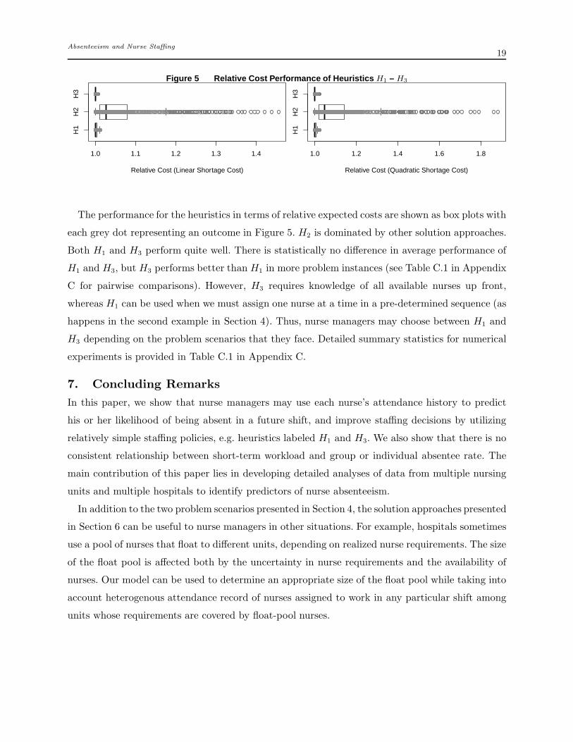
Figure 5 Relative Cost Performance of Heuristics H1 – H3H
1H
2H
3
1.0 1.1 1.2 1.3 1.4
Relative Cost (Linear Shortage Cost)
H1
H2
H3
1.0 1.2 1.4 1.6 1.8
Relative Cost (Quadratic Shortage Cost)
The performance for the heuristics in terms of relative expected costs are shown as box plots with
each grey dot representing an outcome in Figure 5. H2 is dominated by other solution approaches.
Both H1 and H3 perform quite well. There is statistically no difference in average performance of
H1 and H3, but H3 performs better than H1 in more problem instances (see Table C.1 in Appendix
C for pairwise comparisons). However, H3 requires knowledge of all available nurses up front,
whereas H1 can be used when we must assign one nurse at a time in a pre-determined sequence (as
happens in the second example in Section 4). Thus, nurse managers may choose between H1 and
H3 depending on the problem scenarios that they face. Detailed summary statistics for numerical
experiments is provided in Table C.1 in Appendix C.
7. Concluding Remarks
In this paper, we show that nurse managers may use each nurse’s attendance history to predict
his or her likelihood of being absent in a future shift, and improve staffing decisions by utilizing
relatively simple staffing policies, e.g. heuristics labeled H1 and H3. We also show that there is no
consistent relationship between short-term workload and group or individual absentee rate. The
main contribution of this paper lies in developing detailed analyses of data from multiple nursing
units and multiple hospitals to identify predictors of nurse absenteeism.
In addition to the two problem scenarios presented in Section 4, the solution approaches presented
in Section 6 can be useful to nurse managers in other situations. For example, hospitals sometimes
use a pool of nurses that float to different units, depending on realized nurse requirements. The size
of the float pool is affected both by the uncertainty in nurse requirements and the availability of
nurses. Our model can be used to determine an appropriate size of the float pool while taking into
account heterogenous attendance record of nurses assigned to work in any particular shift among
units whose requirements are covered by float-pool nurses.
Absenteeism and Nurse Staffing20
Appendix. A
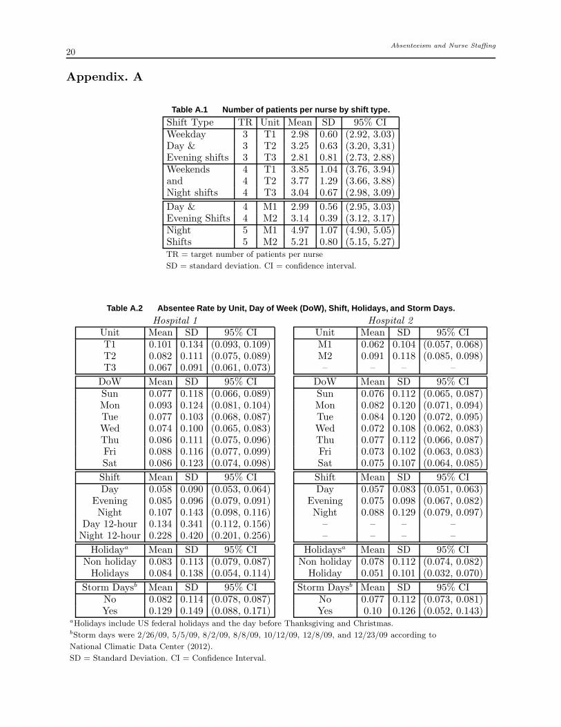
Table A.1 Number of patients per nurse by shift type.
Shift Type TR Unit Mean SD 95% CIWeekday 3 T1 2.98 0.60 (2.92, 3.03)Day & 3 T2 3.25 0.63 (3.20, 3,31)Evening shifts 3 T3 2.81 0.81 (2.73, 2.88)Weekends 4 T1 3.85 1.04 (3.76, 3.94)and 4 T2 3.77 1.29 (3.66, 3.88)Night shifts 4 T3 3.04 0.67 (2.98, 3.09)
Day & 4 M1 2.99 0.56 (2.95, 3.03)Evening Shifts 4 M2 3.14 0.39 (3.12, 3.17)Night 5 M1 4.97 1.07 (4.90, 5.05)Shifts 5 M2 5.21 0.80 (5.15, 5.27)TR = target number of patients per nurse
SD = standard deviation. CI = confidence interval.
Table A.2 Absentee Rate by Unit, Day of Week (DoW), Shift, Hol idays, and Storm Days.
Hospital 1Unit Mean SD 95% CIT1 0.101 0.134 (0.093, 0.109)T2 0.082 0.111 (0.075, 0.089)T3 0.067 0.091 (0.061, 0.073)
DoW Mean SD 95% CISun 0.077 0.118 (0.066, 0.089)Mon 0.093 0.124 (0.081, 0.104)Tue 0.077 0.103 (0.068, 0.087)Wed 0.074 0.100 (0.065, 0.083)Thu 0.086 0.111 (0.075, 0.096)Fri 0.088 0.116 (0.077, 0.099)Sat 0.086 0.123 (0.074, 0.098)
Shift Mean SD 95% CIDay 0.058 0.090 (0.053, 0.064)
Evening 0.085 0.096 (0.079, 0.091)Night 0.107 0.143 (0.098, 0.116)
Day 12-hour 0.134 0.341 (0.112, 0.156)Night 12-hour 0.228 0.420 (0.201, 0.256)
Holidaya Mean SD 95% CINon holiday 0.083 0.113 (0.079, 0.087)Holidays 0.084 0.138 (0.054, 0.114)
Storm Daysb Mean SD 95% CINo 0.082 0.114 (0.078, 0.087)Yes 0.129 0.149 (0.088, 0.171)
Hospital 2Unit Mean SD 95% CIM1 0.062 0.104 (0.057, 0.068)M2 0.091 0.118 (0.085, 0.098)– – – –
DoW Mean SD 95% CISun 0.076 0.112 (0.065, 0.087)Mon 0.082 0.120 (0.071, 0.094)Tue 0.084 0.120 (0.072, 0.095)Wed 0.072 0.108 (0.062, 0.083)Thu 0.077 0.112 (0.066, 0.087)Fri 0.073 0.102 (0.063, 0.083)Sat 0.075 0.107 (0.064, 0.085)
Shift Mean SD 95% CIDay 0.057 0.083 (0.051, 0.063)
Evening 0.075 0.098 (0.067, 0.082)Night 0.088 0.129 (0.079, 0.097)– – – –– – – –
Holidaysa Mean SD 95% CINon holiday 0.078 0.112 (0.074, 0.082)Holiday 0.051 0.101 (0.032, 0.070)
Storm Daysb Mean SD 95% CINo 0.077 0.112 (0.073, 0.081)Yes 0.10 0.126 (0.052, 0.143)
aHolidays include US federal holidays and the day before Thanksgiving and Christmas.bStorm days were 2/26/09, 5/5/09, 8/2/09, 8/8/09, 10/12/09, 12/8/09, and 12/23/09 according to
National Climatic Data Center (2012).
SD = Standard Deviation. CI = Confidence Interval.
Absenteeism and Nurse Staffing21
Appendix. B
Proof for Proposition 1
Note that Xi ≤icx X′
ifor each i= 1, · · · ,m. Therefore, E[c0(Xi −Qi(a))
+]≤ E[c0(X′
i−Qi(a))
+] for each i
and π(a∗
X) =
∑
u
i=1E[c0(Xi−Qi(a∗
X)+]≤
∑
u
i=1E[c0(Xi−Qi(a∗
X′)+]≤
∑
u
i=1E[c0(X′
i−Qi(a
∗
X′)+] = π(a∗
X′).
Proof of Proposition 2
The result of Proposition 2 comes from a property of Schur-convex functions (Marshall et al. 2011). Let g(qi) =
E[co(Xi− qi)+], where qi is the (deterministic) number of nurses who show up in unit i. It is straightforward
to verify that g(·) is convex in qi. Suppose q ≤M q′, then∑
k
i=1 g(qi)≤∑
k
i=1 g(q′
i) ∀ k = 1, · · · , n. Also, let
q= (1/u)∑
u
i=1 qi. The inequality∑
u
i=1 g(q)≤∑
u
i=1 g(qi) holds for all convex functions (Marshall et al. 2011).
Note that each unit’s demand are independent and identically distributed, therefore the cost function
πi(a) =E[c0(Xi − qi)+] is the same convex cost function (convex in qi) for all i. Based on the above Schur-
convex function property, the best expected shortage cost (π(a∗) =∑
u
i=1 πi(a∗)) is achieved when each unit’s
staffing level is equal (i.e. qi =Qi(a) =∑
m
t=1 a(i)t −φi(a) = q ∀ i= 1, · · · ,m.) See, Muller and Stoyan (2002).
Proof of Proposition 3
Let π(a) =∑
u
i=1 πi(a(i)). Because Yi ≤icx Y ′
i, πi(a
(i)|Y ) = E[c0(Xi −∑
m
t=1 a(i)t + a
(i)t Yi))
+] ≤ E[c0(Xi −∑
m
t=1 a(i)t +a
(i)t Y ′
i))+] = πi(a
(i)|Y ′) for each i. Therefore π(a∗
Y) = π(a∗
Y|Y )≤ π(a∗
Y ′ |Y )≤ π(a∗
Y ′ |Y ′) = π(a∗
Y ′).
Proof of Proposition 4
{B(pt), p∈ (0,1)} is a family of independent random variables parameterized by pt. Let Ft(k, pt) = P (B(pt)>
k). Because Ft(k, pt) is convex linear in pt for each fixed k, B(pt) is SIL(st) – see Shaked and Shanthikumar
(2007) for details. Next, we observe that the function h(b) = x+∑
n
t=1 b(i)t −mi, where x is a realization
of random demand Xi, b(i)t is a realization of B(p
(i)t ), p
(i)t is the t-th element of vector p(i), and mi is
the cardinality of the vector p(i), is an increasing valuation in b. A function is said to be a valuation if
it is both sub- and supermodular (Topkis 1998). Define Z(p) = h(B(p(i)1 ), · · · ,B(p(i)
mi)). Then, it follows
immediately that {Z(p),p(i) ∈ (0,1)n} is SI-SchurCX(icx) – see Liyanage and Shanthikumar (1992, The-
orem 2.12). This theorem also implies that for an increasing convex function g, p(i) ≤M p′(i) implies that
E[g(h(B(p′(i)1 ), · · · ,B(p′(i)
mi)))]≤E[g(h(B(p
(i)1 ), · · · ,B(p(i)
mi)))]. The statement of the proposition then follows
from the fact that c0(·) is an increasing convex function.
Appendix. C
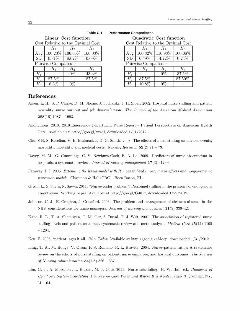
The left (resp. right) panel shows the performance comparisons under a linear (resp. quadratic) cost
function. Within each panel, the upper table reports the mean and standard deviation of the ratio of the
cost associated with each heuristic and the optimal cost, expressed in percent. Each cell in the lower table
summarizes the percent of scenarios in which the column strategy performed better than the row strategy.
Absenteeism and Nurse Staffing22
Table C.1 Performance Comparisons
Linear Cost function
Cost Relative to the Optimal CostH1 H2 H3
Avg 100.23% 106.05% 100.03%SD 0.31% 8.02% 0.09%Pairwise Comparisons
H1 H2 H3
H1 – 0% 43.3%H2 87.5% – 87.5%H3 6.3% 0% –
Quadratic Cost function
Cost Relative to the Optimal CostH1 H2 H3
Avg 100.32% 110.93% 100.08%SD 0.49% 14.72% 0.24%Pairwise Comparisons
H1 H2 H3
H1 – 0% 37.1%H2 87.5% – 87.50%H3 10.8% 0% –
References
Aiken, L. H., S. P. Clarke, D. M. Sloane, J. Sochalski, J. H. Siber. 2002. Hospital nurse staffing and patient
mortality, nurse burnout and job dissatisfaction. The Journal of the American Medical Association
288(16) 1987 – 1993.
Anonymous. 2010. 2010 Emergency Department Pulse Report – Patient Perspectives on American Health
Care. Available at: http://goo.gl/vz4eI, downloaded 1/31/2012.
Cho, S-H, S. Ketefian, V. H. Barkauskas, D. G. Smith. 2003. The effects of nurse staffing on adverse events,
morbidity, mortality, and medical costs. Nursing Research 52(2) 71 – 79.
Davey, M. M., G. Cummings, C. V. Newburn-Cook, E. A. Lo. 2009. Predictors of nurse absenteeism in
hospitals: a systematic review. Journal of nursing management 17(3) 312–30.
Faraway, J. J. 2006. Extending the linear model with R – generalized linear, mixed effects and nonparametric
regression models . Chapman & Hall/CRC – Boca Raton, FL.
Green, L., S. Savin, N. Savva. 2011. “Nursevendor problem”: Personnel staffing in the presence of endogenous
absenteeism. Working paper. Available at http://goo.gl/G401z, downloaded 1/29/2012.
Johnson, C. J., E. Croghan, J. Crawford. 2003. The problem and management of sickness absence in the
NHS: considerations for nurse managers. Journal of nursing management 11(5) 336–42.
Kane, R. L., T. A. Shamliyan, C. Mueller, S. Duval, T. J. Wilt. 2007. The association of registered nurse
staffing levels and patient outcomes. systematic review and meta-analysis. Medical Care 45(12) 1195
– 1204.
Ken, F. 2006. ‘patient’ says it all. USA Today Available at http://goo.gl/nMqcp, downloaded 1/31/2012.
Lang, T. A., M. Hodge, V. Olson, P. S. Romano, R. L. Kravitz. 2004. Nurse–patient ratios: A systematic
review on the effects of nurse staffing on patient, nurse employee, and hospital outcomes. The Journal
of Nursing Administration 34(7-8) 326 – 337.
Lim, G. J., A. Mobasher, L. Kardar, M. J. Cote. 2011. Nurse scheduling. R. W. Hall, ed., Handbook of
Healthcare System Scheduling: Deliverying Care When and Where It is Needed , chap. 3. Springer, NY,
31 – 64.
Absenteeism and Nurse Staffing23
Liyanage, L., J. G. Shanthikumar. 1992. Allocation through stochastic schur convexity and stochastic trans-
position increasingness. Lecture Notes-Monograph Series 22 pp. 253–273.
Marshall, A. W., I. Olkin, B. C. Arnold. 2011. Inequalities: Theory of Majorization and Its Applications .
2nd ed. Springer, NY.
Muller, A., D. Stoyan. 2002. Comparison Methods for Stochastic Models and Risks . John Wiley & Sons:
New York, NY.
National Center for Health Statistics. 2011. Health, United States, 2010: With Special Feature on Death
and Dying. Available at http://www.cdc.gov/nchs/data/hus/hus10.pdf, downloaded 1/31/2012.
National Climatic Data Center. 2012. NCDC Storm Event Database. Data available at http://goo.gl/V3zWs,
downloaded 1/12/2012.
Needleman, J., P. Buerhaus, S. Mattke, M. Stewart, K. Zelevinsky. 2002. Nurse-staffing levels and the quality
of care in hospitals. The New England Journal of Medicine 346(22) 1715 – 1722.
Shaked, M., J. G. Shanthikumar. 2007. Stochastic orders . New York : Springer.
Topkis, D. 1998. Supermodularity and complementarity. 2nd ed. Princeton University Press, New Jersey.
Unruh, L. 2008. Nurse staffing and patient, nurse, and financial outcomes. American Journal of Nursing
108(1) 62–71.
Yano, C. A., H. L. Lee. 1995. Lot sizing with random yields: A review. Operations Research 43(2) pp.
311–334.
Zeger, S. L., K-Y. Liang. 1986. Longitudinal data analysis for discrete and continuous outcomes. Biometrics
42(1) 121 – 130.